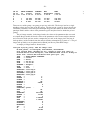
1
A Reference Guide to the IRAF/DAOPHOT Package
Lindsey E. Davis
IRAF Programming Group
National Optical Astronomy Observatories††
Tucson, Arizona 85726
January 1994
ABSTRACT
DAOPHOT is a software package for doing stellar photometry in crowded
stellar fields developed by Peter Stetson (1987) of the Dominion Astrophysical
Observatory. IRAF/DAOPHOT uses the task structure and algorithms of DAOPHOT to do crowded-field stellar photometry within the IRAF data reduction
and analysis environment.
This document briefly describes the principal similarities and differences
between DAOPHOT and IRAF/DAOPHOT, the data preparation required to
successfully use IRAF/DAOPHOT, how to examine and edit the
IRAF/DAOPHOT algorithm parameters, how to run the IRAF/DAOPHOT
package tasks interactively, non-interactively, or in the background, and how to
examine and perform simple database operations on the output photometry files.
This document is intended as a reference guide to the details of using and
interpreting the results of IRAF/DAOPHOT not a user’s cookbook or a general
guide to doing photometry in IRAF. Its goal is to take the user from a fully
reduced image of a crowded stellar field to aperture corrected instrumental magnitudes using a small artificial image as a sample data set. First time
IRAF/DAOPHOT users should consult A User’s Guide to Stellar Photometry
With IRAF, by Phil Massey and Lindsey Davis. Detailed descriptions of the
DAOPHOT photometry algorithms can be found in Stetson (1987, 1990, 1992).
††Operated by the Association of Universities for Research in Astronomy, Inc. under cooperative
agreement with the National Science Foundation.
Contents
1.
Introduction................................................................................................................
1
2.
DAOPHOT and IRAF/DAOPHOT ..........................................................................
1
3.
Preparing Data for DAOPHOT................................................................................
3
4.
Some IRAF Basics for New IRAF and DAOPHOT Users .....................................
4
4.1.
Pre-loaded Packages .....................................................................................
4.1.1.
The DATAIO Package.....................................................................
4.1.2.
The PLOT Package..........................................................................
4.1.3.
The IMAGES Package ....................................................................
4.1.4.
The TV Package ..............................................................................
Other Useful Packages and Tasks ...............................................................
Image Types, Image Directories, and Image Headers ...............................
The Image Display and Image Cursor ........................................................
The Graphics Device and Graphics Cursor ...............................................
4
5
5
5
5
5
5
6
7
Some DAOPHOT Basics for New DAOPHOT Users .............................................
8
4.2.
4.3.
4.4.
4.5.
5.
5.1.
5.2.
5.3.
5.4.
5.5.
5.6.
5.7.
5.8.
5.9.
5.10.
5.11.
5.12.
5.13.
5.14.
5.15.
6.
Loading the DAOPHOT Package................................................................
Loading the TABLES Package ....................................................................
Running the Test Script ...............................................................................
On-line Help ..................................................................................................
Editing the Package Parameters..................................................................
Editing the Task Parameters .......................................................................
Input and Output Image Names..................................................................
Input and Output File Names......................................................................
Algorithm Parameter Sets ...........................................................................
Interactive Mode and Non-Interactive Mode ............................................
Image and Graphics Cursor Input ..............................................................
Graphics Output ...........................................................................................
Verify, Update, and Verbose........................................................................
Background Jobs...........................................................................................
Timing Tests ..................................................................................................
8
8
8
9
10
11
11
12
12
14
14
15
15
15
16
Doing Photometry with DAOPHOT......................................................................... 16
6.1.
6.2.
6.3.
6.4.
6.5.
6.6.
The Test Image..............................................................................................
Typical Analysis Sequence ...........................................................................
Creating and Organizing an Analysis Directory........................................
Reading the Data ..........................................................................................
Editing the Image Headers...........................................................................
6.5.1.
The Minimum Image Header Requirements....................................
6.5.2.
The Effective Gain and Readout Noise ...........................................
6.5.3.
The Maximum Good Data Value ....................................................
6.5.4.
The Effective Exposure Time ..........................................................
6.5.5.
The Airmass, Filter Id, and Time of Observation ...........................
6.5.6.
Batch Header Editing.......................................................................
Editing, Checking, and Storing the Algorithm Parameters......................
6.6.1.
The Critical Algorithm Parameters..................................................
6.6.2.
Editing the Algorithm Parameters Interactively with Daoedit .......
16
17
19
19
19
19
19
21
22
22
24
24
24
24
6.7.
6.8.
6.9.
6.10.
6.6.2.1.
The Data Dependent Algorithm Parameters .................
6.6.2.2.
The Centering Algorithm Parameters ............................
6.6.2.3.
The Sky Fitting Algorithm Parameters..........................
6.6.2.4.
The Aperture Photometry Parameters............................
6.6.2.5.
The Psf Modeling and Fitting Parameters .....................
6.6.2.6.
Setting the Algorithm Parameters Graphically ..............
6.6.3.
Checking the Algorithm Parameters with Daoedit ..........................
6.6.4.
Storing the Algorithm Parameter Values with Setimpars................
6.6.5.
Restoring the Algorithm Parameter Values with Setimpars ............
Creating a Star List ......................................................................................
6.7.1.
The Daofind Task ............................................................................
6.7.1.1.
The Daofind Algorithm .................................................
6.7.1.2.
The Daofind Algorithm Parameters...............................
6.7.1.3.
Running Daofind Non-Interactively...............................
6.7.1.4.
Running Daofind Interactively.......................................
6.7.1.5.
The Daofind Output .......................................................
6.7.1.6.
Examining the Daofind Output......................................
6.7.2.
Rgcursor and Rimcursor ..................................................................
6.7.3.
User Program...................................................................................
6.7.4.
Modifying an Existing Coordinate List ...........................................
Initializing the Photometry with Phot .........................................................
6.8.1.
The Phot Algorithm.........................................................................
6.8.2.
The Phot Algorithm Parameters ......................................................
6.8.3.
Running Phot Non-interactively ......................................................
6.8.4.
Running Phot Interactively ..............................................................
6.8.5.
The Phot Output ..............................................................................
6.8.6.
Examining the Results of Phot ........................................................
Creating a Psf Star List with Pstselect........................................................
6.9.1.
The Pstselect Algorithm ..................................................................
6.9.2.
The Pstselect Algorithm Parameters................................................
6.9.3.
How Many Psf Stars Should Be Selected ?.....................................
6.9.4.
Running Pstselect Non-interactively................................................
6.9.5.
Running Pstselect Interactively........................................................
6.9.6.
The Pstselect Output........................................................................
6.9.7.
Examining and/or Editing the Results of Pstselect..........................
Computing the Psf Model with Psf..............................................................
6.10.1. The Psf Algorithm ...........................................................................
6.10.2. Choosing the Appropriate Analytic Function ..................................
6.10.3. The Analytic Psf Model...................................................................
6.10.4. The Empirical Constant Psf Model .................................................
6.10.5. The Empirical Variable Psf Model ..................................................
6.10.6. Rejecting Bad Data from the Psf Model .........................................
6.10.7. The Model Psf Psfrad and Fitrad.....................................................
6.10.8. Modeling the Psf Interactively Without a Psf Star List...................
6.10.9. Fitting the Psf Model Interactively Using an Initial Psf Star List...
6.10.10. Fitting the Psf Model Interactively Without an Image Display.......
6.10.11. Fitting the Psf Model Non-interactively..........................................
6.10.12. The Output of Psf ............................................................................
6.10.13. Checking the Psf Model ..................................................................
6.10.14. Removing Bad Stars from the Psf Model........................................
6.10.15. Adding New Stars to a Psf Star Group............................................
6.10.16. Refitting the Psf Model With the New Psf Star Groups..................
6.10.17. Computing the Final Psf Model ......................................................
6.10.18. Visualizing the Psf Model with the Seepsf Task.............................
25
28
29
29
30
31
31
32
32
32
33
33
33
34
34
36
37
38
39
39
39
39
40
40
42
43
44
44
45
45
46
47
47
48
48
49
49
50
50
51
51
51
52
52
54
55
56
57
59
62
62
62
63
63
6.11.
6.12.
6.13.
6.14.
6.15.
6.16.
6.17.
6.18.
6.19.
6.10.19. Problems Computing the Psf Model................................................
Doing Psf Fitting Photometry with Peak, Nstar, or Allstar .....................
6.11.1. Fitting Single Stars with Peak .........................................................
6.11.1.1. The Peak Algorithm.......................................................
6.11.1.2. Running Peak ...............................................................
6.11.1.3. The Peak Output ............................................................
6.11.2. Fitting Stars with Group, Grpselect, Nstar and Substar ..................
6.11.2.1. The Group and Nstar Algorithms ..................................
6.11.2.2. Running Group, Grpselect, and Nstar............................
6.11.2.3. The Nstar Output ...........................................................
6.11.3. Fitting Stars With Allstar ................................................................
6.11.3.1. The Allstar Algorithm ...................................................
6.11.3.2. Running Allstar..............................................................
6.11.3.3. The Allstar Output .........................................................
Examining the Output Photometry Files ....................................................
Problems with the Photometry.....................................................................
Detecting Stars Missed By Daofind .............................................................
Initializing the Missing Star Photometry with Phot ..................................
Merging Photometry Files with Pfmerge ....................................................
Refitting the Stars with Allstar ....................................................................
Examining the Subtracted Image ................................................................
Computing an Aperture Correction............................................................
64
65
65
65
65
66
67
67
68
70
71
71
72
73
73
74
75
75
76
76
76
76
7.
References...................................................................................................................
77
8.
Appendices..................................................................................................................
77
8.1.
8.2.
8.3.
8.4.
8.5.
8.6.
8.7.
8.8.
77
77
78
78
78
78
79
79
The Instrumental Magnitude Scale .............................................................
The Analytic Psf Models...............................................................................
The Error Model ...........................................................................................
The Radial Weighting Function ..................................................................
Total Weights ................................................................................................
Bad Data Detection .......................................................................................
Stellar Mergers..............................................................................................
Faint Stars......................................................................................................
A Reference Guide to the IRAF/DAOPHOT Package
Lindsey E. Davis
IRAF Programming Group
National Optical Astronomy Observatories††
Tucson, Arizona 85726
January 1994
1. Introduction
DAOPHOT is a software package for doing stellar photometry in crowded fields
developed by Peter Stetson of the DAO (1987, 1990, 1992). The IRAF/DAOPHOT package
uses the task structure and algorithms of DAOPHOT to do crowded field photometry within the
IRAF data reduction and analysis environment.
Input to IRAF/DAOPHOT consists of an IRAF image file, numerous parameters controlling the analysis algorithms and, optionally, graphics cursor and/or image display cursor input.
IRAF/DAOPHOT produces output photometry files in either text format or STSDAS binary
table format. Some IRAF/DAOPHOT tasks also produce image output and graphics output in
the form of plot metacode files.
Separate tasks are provided for examining, editing, storing, and recalling the analysis
parameters, creating and editing star lists, computing accurate centers, sky values and initial
magnitudes for the stars in the list, computing the point-spread function, grouping the stars into
physical associations, fitting the stars either singly or in groups, subtracting the fitted stars from
the original image, and adding artificial test stars to the original image. A set of tools are also
provided for examining and editing the output photometry files.
2. DAOPHOT and IRAF/DAOPHOT
The principal similarities and differences between DAOPHOT and IRAF/DAOPHOT are
summarized below.
[1] The structure of IRAF/DAOPHOT is very similar to the structure of DAOPHOT. All the
DAOPHOT photometry tasks and many of the utilities tasks are present in
IRAF/DAOPHOT and in many cases the DAOPHOT task names have been preserved. A
listing of the DAOPHOT photometry tasks and their closest IRAF/DAOPHOT equivalents
is shown below.
DAOPHOT
TASK
IRAF/DAOPHOT
EQUIVALENT
add*
allstar
attach
append
addstar
allstar
N/A
pfmerge,pconcat
††Operated by the Association of Universities for Research in Astronomy, Inc. under cooperative
agreement with the National Science Foundation.
-2find
group
monitor
nomonitor
nstar
offset
options
peak
photometry
pick
psf
select
sort
sub*
[2]
[3]
[4]
[5]
[6]
[7]
daofind
group
daophot.verbose=yes
daophot.verbose=no
nstar
pcalc
daoedit
peak
phot
pstselect
psf
grpselect
psort,prenumber
substar
Some DAOPHOT utilities tasks are missing from IRAF/DAOPHOT. The DAOPHOT
tasks dump, exit, fudge, help, list, and sky have been replaced with general IRAF tasks,
or with IRAF system facilities that perform the equivalent function. The missing DAOPHOT utilities tasks and their IRAF equivalents are shown below.
DAOPHOT
TASK
IRAF/DAOPHOT
EQUIVALENT
dump
exit
fudge
help
list
sky
listpixels,imexamine
bye
imreplace,fixpix,imedit
help daophot
imheader
imstatistics,phistogram,imexamine
The IRAF/DAOPHOT default algorithms are the DAOPHOT II algorithms (Stetson 1992).
Users have more choice of and control over the algorithms in IRAF/DAOPHOT than they
do in DAOPHOT. For example the IRAF/DAOPHOT aperture photometry task phot
offers several sky fitting algorithms besides the default "mode" algorithm, and full control
over the sky fitting algorithm parameters.
The algorithm parameters in IRAF/DAOPHOT are grouped by function into six parameter
sets or psets rather than three as in DAOPHOT. The six IRAF/DAOPHOT parameter sets
with their DAOPHOT equivalents in brackets are: 1) datapars, the data definition parameters (daophot.opt), 2) findpars, the detection algorithm parameters (daophot.opt), 3) centerpars, the aperture photometry centering algorithm parameters (no equivalent), 4)
fitskypars, the aperture photometry sky fitting parameters (photo.opt), 5) photpars, the
aperture photometry parameters (photo.opt), 6) daopars, the IRAF/DAOPHOT psf fitting
parameters (daophot.opt, allstar.opt).
The IRAF/DAOPHOT algorithm parameter sets unlike the DAOPHOT parameter sets can
be interactively examined, edited and saved with the daoedit task using the image display
and radial profile plots.
The IRAF/DAOPHOT algorithm parameter sets unlike the DAOPHOT parameter sets can
be saved and restored as a function of image using the setimpars task.
-3[8]
[9]
[10]
[11]
[12]
[13]
[14]
Memory allocation in IRAF/DAOPHOT is dynamic not static as in DAOPHOT.
IRAF/DAOPHOT allocates and frees memory as required at run-time subject to the physical memory and swap space limitations of the host computer.
The IRAF/DAOPHOT point-spread function look-up table is stored in an IRAF image not
an ASCII table as in DAOPHOT.
Unlike DAOPHOT, the IRAF/DAOPHOT tasks daofind, phot, pstselect and psf can be
run interactively using the image display and graphics window or non-interactively.
Display and graphics capabilities were deliberately omitted from DAOPHOT to minimize
portability problems.
The IRAF/DAOPHOT output photometry files can be written in either text format as in
DAOPHOT or STSDAS binary table format.
Unlike DAOPHOT, fields or columns in both IRAF/DAOPHOT text and STSDAS binary
table photometry files are identified by name and have an associated units and format
specifier. The IRAF/DAOPHOT photometry file input routines search for column names,
for example "GROUP,ID,XCENTER,YCENTER,MAG,MSKY" as appropriate but are
independent of their placement in the input file.
Several general purpose IRAF/DAOPHOT tasks are available for performing operations on
the final output photometry catalogs. In addition to pcalc, pconcat, pfmerge, prenumber,
and psort which are also available in DAOPHOT, there are three photometry file editing
tasks which have no analog in DAOPHOT pdump, pexamine, and pselect. All these
tasks work on IRAF/DAOPHOT output text files or STSDAS binary tables. An
IRAF/DAOPHOT task is supplied for converting output text files to STSDAS binary
tables so as to make use of the even more general STSDAS tables manipulation tools in
the TABLES package.
The IRAF/DAOPHOT output files are self-documenting. All the information required to
comprehend the history of or decode the output photometry file is in the file itself, including the IRAF version number, host computer, date, time, and names of all the input and
output files and the values of all the parameters.
For the remainder of this document IRAF/DAOPHOT will be referred to as DAOPHOT.
3. Preparing Data for DAOPHOT
[1]
[2]
[3]
[4]
DAOPHOT assumes that the images to be analyzed exist on disk in IRAF image format.
DAOPHOT can read and write old IRAF format ".imh" images and ST IRAF format
".hhh" images. When the IRAF FITS kernel becomes available DAOPHOT will be able
to read FITS images on disk as well. QPOE IRAF format ".qp" images must be rasterized
before they can be input to DAOPHOT.
All internal DAOPHOT calculations are done in real precision. The pixel type of the
image data on disk may be any of the following data types: short integer, unsigned short
integer, integer, long integer, real or double. Users should realize that the extra precision
in images of type double will not be used by DAOPHOT.
The instrumental signature must be removed from the input images prior to running DAOPHOT. All CCD images should be overscan corrected, bias corrected, dark current
corrected and flat-fielded. Users should be aware of the IRAF CCDRED package for
reducing CCD data.
DAOPHOT assumes that the input pixel data is linear. If the data is non-linear over a
large fraction of its total dynamic range, the data must be linearized before running DAOPHOT.
-4[5]
Saturated pixels or pixels distinguishable from good data by intensity, do not need to be
removed from the image prior to running DAOPHOT. For example if the data is nonlinear only above 25000 counts, DAOPHOT can be instructed to ignore pixels above
25000 counts.
[6] Extreme-valued pixels should be removed from the images prior to running DAOPHOT.
Extreme-valued pixels include those with values at or near the floating point limits of the
host machine and host machine special numbers produced by operations like divide by
zero, floating point underflows and overflows, etc. The latter category of extreme-valued
pixels should not be produced by IRAF software, but may be produced by user programs
including imfort programs. Floating point operations involving such numbers will frequently cause arithmetic exception errors, since for efficiency and portability reasons the
DAOPHOT package and most IRAF tasks do not test for their presence. The imreplace
task in the PROTO package can be used to remove extreme- valued pixels.
[7] The background sky value should NOT be subtracted from the image prior to entering the
DAOPHOT package. The DAOPHOT fitting routines use an optimal weighting scheme
which depends on the readout noise, the gain, and the true counts in the pixels. If the
mean sky has been subtracted then the counts in the image are not the true counts and the
computed weights will be incorrect. For similar reasons users should not attempt to correct
their magnitudes for exposure time by dividing their images by the exposure time.
[8] Cosmic ray and bad pixel removal programs should be used with caution. If the data and
parameter values are set such that the cosmic ray and bad pixel detection and removal
algorithms have difficulty distinguishing between stars and bad pixels or cosmic rays, the
peaks of the stars may be clipped, altering the point-spread function and introducing errors
into the photometry.
[9] DAOPHOT assumes that the local sky background is approximately flat in the vicinity of
the object being measured. This assumption is equivalent to requiring that the local sky
region have a unique mode. Variations in the sky background which occur on the same
scale as the size of the local sky region will introduce errors into the photometry.
[10] The point spread function must be constant or smoothly varying with position over the
entire image. This is the fundamental assumption underlying all of DAOPHOT. All stars
in the image must be indistinguishable except for position and magnitude. The variable
point spread function option is capable of handling second order variability as a function
of position in the image.
[11] The input images should not have undergone any operations which fundamentally alter the
image point spread function or the image statistics in a non-linear way. For example, nonlinear image restoration tasks must not be run on the image to prior to running DAOPHOT.
[12] The gain, readout noise, exposure time, airmass, filter, and observing time should be
present and correct in the image headers before DAOPHOT reductions are begun. DAOPHOT tasks can extract this information from the image headers, use it in the computations, and/or store it in the output photometry files, greatly simplifying the analysis and
subsequent calibration procedures.
4. Some IRAF Basics for New IRAF and DAOPHOT Users
4.1. Pre-loaded Packages
Under IRAF versions 2.10 and later the DATAIO, PLOT, IMAGES, TV and NOAO packages are pre-loaded so that all the tasks directly under them are available when IRAF is started.
Each of these packages contains tasks which are useful to DAOPHOT users for various reasons,
-5and each is discussed briefly below.
4.1.1. The DATAIO Package
DAOPHOT users should be aware of the DATAIO rfits and wfits tasks which are used to
transport data into and out of IRAF. Any input and output images, including point-spread function look-up table images, should normally be archived with wfits. The cardimage reader and
writer tasks for archiving text files, rcardimage and wcardimage, are also located here.
4.1.2. The PLOT Package
Various general purpose image and file plotting utilities can be found in the PLOT packages. DAOPHOT users should be aware of the interactive image row and column plotting task
implot, the image contour plotting task contour, the image surface plotting task surface, image
histogram plotting task phistogram, the image radial profile plotting task pradprof, and the
general purpose graphing tool graph. The tasks gkidir and gkiextract are also useful for
extracting individual plots from the plot metacode files which may be produced by some DAOPHOT tasks.
4.1.3. The IMAGES Package
The IMAGES package contains a set of general purpose image operators. DAOPHOT
users should be aware of the image header examining tasks imheader and hselect, the header
editing task hedit, the coordinate and pixel value dumping task listpixels, and the image statistics task imstatistics.
4.1.4. The TV Package
The TV package contains tasks which interact with the image display including the all
important display task for displaying images, the interactive image examining task imexamine,
and the tvmark task for marking objects on the image display. DAOPHOT users should
become familiar with all three of these tasks.
4.2. Other Useful Packages and Tasks
The NPROTO package contains two useful tasks, findgain, for computing the gain and
readout noise of a CCD from a pair of biases and flats, and findthresh for computing the standard deviation of the background in a CCD frame given the readout noise and gain. The ASTUTIL package contains the setairmass task for computing and/or correcting the airmass given the
appropriate input data. Users might also wish to experiment with the tasks in the artificial data
package ARTDATA, and run the resulting images through DAOPHOT.
4.3. Image Types, Image Directories, and Image Headers
The IRAF image environment is controlled by several environment variables. The most
important of these for DAOPHOT users are: imtype the disk image format, imdir the default
pixel directory, and min_lenuserarea the maximum length of the image header. The values of
-6these environment variables can be listed as shown below.
cl> show imtype
imh
cl> show imdir
/data/davis/pixels/
cl> show min_lenuserarea
24000
"imh" is the default image format for most IRAF users, "hhh" the default image format
for ST users, and "qp" the photon counting format used for photon counting data. DAOPHOT
will work transparently on "imh" and "hhh" images. "qp" event lists must be rasterized prior to
using DAOPHOT. When IRAF supports FITS images on disk, image format "fits", DAOPHOT
will be able to work directly on FITS images as well. IRAF uses the image name extension, e.g.
"imh" to automatically sense the image disk format on input. The output disk format is set by:
1) the extension of the output image name if present e.g. "imh", 2) the cl environment variable
imtype if the output image is opened as a new image, e.g. the output of the rfits task, 3) the
type of the input image if the output image is opened as a new copy of an existing image, e.g.
the output of the imcopy task.
imdir specifies the default image pixel directory for "imh" format files. The image header
files are written to the current directory and the pixel files are written to imdir. imdir can be set
to an existing directory on a scratch disk, the current directory "HDR$", or the subdirectory pixels under the current directory "HDR$pixels/". DAOPHOT users should keep both the intrinsic
speed of a disk and its network configuration in mind when setting imdir.
min_lenuserarea is the size of the image header area reserved in memory when a new or
existing image is opened. The current default value of 24000 corresponds to space for approximately 300 keywords. If an image on disk has a header larger than this the image header will
be truncated when it is read. For most DAOPHOT users the default value is sufficient. However users whose images have large headers or who are creating a point-spread function using
more than ~70 stars should set min_lenuserarea to a larger value, e.g. 40000.
The following example shows how to change the default pixel directory to HDR$pixels/
and set min_lenuserarea to 40000. To avoid redefining these quantities for every session, users
should enter the redefinitions into their login.cl or loginuser.cl files.
cl> reset imdir = "HDR$pixels/"
cl> reset min_lenuserarea = 40000
4.4. The Image Display and Image Cursor
Several DAOPHOT tasks are interactive tasks or have an interactive as well as a noninteractive mode. In interactive mode these tasks must be able to read the image cursor on a
displayed image and perform various actions depending on the position of the image cursor and
the keystroke command typed.
DAOPHOT will work with the display servers Imtool, Saoimage, and Ximtool. DAOPHOT users should be aware that both Imtool and Ximtool support multiple frame buffers while
SAOimage does not. Multiple frame buffers are an important feature for users who wish to
compare their original images with the DAOPHOT output images from which all the fitted stars
have been subtracted. Users running DAOPHOT on a remote machine, e.g. one with lots of
memory and/or disk space, but displaying on their local machine also need to set the node
environment variable to the name of the local machine.
-7cl> show node
ERROR: No such environment variable
show (node)
cl> set node = mymachine
The maximum size of the display server frame buffer is defined by the environment variable stdimage whose value can be printed as shown below.
cl> show stdimage
imt512
In the previous example the default frames buffers are 512 pixels square. A user whose images
are 2K square will want to reset the default frame buffer size as shown below.
cl> reset stdimage = imt2048
cl> show stdimage
imt2048
In order for image cursor read-back to function correctly the environment variable stdimcur must be set to "stdimage" as shown below.
cl> show stdimcur
stdimage
To check that image cursor read-back is functioning correctly the user should display an image
and try to bring up the image display cursor as shown below.
cl> display image 1
cl> =imcur
The image cursor should appear on the image display reading the correct image pixel coordinates and ready to accept a keystroke command. Any keystroke will terminate the cursor read.
4.5. The Graphics Device and Graphics Cursor
Some interactive DAOPHOT tasks have graphics submenus which require them to be able
to read the graphics cursor on for example a radial profile plot and perform various actions
based on the position of the graphics cursor in the plot and the keystroke command issued. The
default graphics device is determined by the stdgraph environment variable as shown below.
cl> show stdgraph
xgterm
To check that graphics cursor read-back is functioning correctly the user should draw a plot and
try to bring up the graphics cursor as shown below.
cl> contour image
cl> =gcur
The graphics cursor should appear in the graphics window ready to accept a keystroke command. Any keystroke will terminate the cursor read.
-85. Some DAOPHOT Basics for New DAOPHOT Users
5.1. Loading the DAOPHOT Package
The DAOPHOT package is located in the digital stellar photometry package DIGIPHOT.
To load DIGIPHOT and DAOPHOT the user types the package names in sequence as shown
below,
cl> digiphot
di> daophot
after which the following menu of tasks appears.
addstar
allstar
centerpars@
daoedit
daofind
daopars@
daotest
datapars@
findpars@
fitskypars@
group
grpselect
nstar
pcalc
pconcat
pconvert
pdump
peak
pexamine
pfmerge
phot
photpars@
prenumber
pselect
psf
psort
pstselect
seepsf
setimpars
substar
Task names with a trailing "@" are parameter set tasks. The remaining tasks are script and/or
compiled tasks. After the DAOPHOT package is loaded the user can redisplay the package
menu at any time with the command.
da> ? daophot
5.2. Loading the TABLES Package
The DAOPHOT photometry tasks write their output photometry files in either text format
(the default) or ST binary tables format. Users wishing to use the ST binary tables format
should acquire and install the ST TABLES external package. Without the TABLES package the
DAOPHOT photometry tasks will read and write ST binary tables, but DAOPHOT utilities like
psort which call TABLES package tasks will not run on ST binary tables.
When DAOPHOT is loaded, it checks to see if the TABLES package is defined, and if so
loads it. A warning message is issued if the TABLES package is undefined. The TABLES package tasks can be listed at any time after DAOPHOT is loaded with the following command.
da> ? tables
5.3. Running the Test Script
The DAOPHOT package includes a script task daotest which executes each of the core
DAOPHOT photometry tasks in turn using a test image stored in FITS format in the DAOPHOT test directory. Daotest is run as shown below.
da> daotest
DAOTEST INITIALIZES THE DAOPHOT TASK PARAMETERS
TYPE ’q’ or ’Q’ TO QUIT, ANY OTHER KEY TO PROCEED
Name of the output test image: test
-9INITIALIZE THE DAOPHOT PACKAGE
TESTING
TESTING
TESTING
TESTING
TESTING
TESTING
TESTING
TESTING
TESTING
TESTING
TESTING
TESTING
THE
THE
THE
THE
THE
THE
THE
THE
THE
THE
THE
THE
DAOFIND TASK
PHOT TASK
PSTSELECT TASK
PSF TASK
PEAK TASK
GROUP TASK
GRPSELECT TASK
NSTAR TASK
ALLSTAR TASK (CACHE=YES)
ALLSTAR TASK (CACHE=NO)
SUBSTAR TASK
ADDSTAR TASK
DAOPHOT PACKAGE TESTS COMPLETED
On task completion the user will find the input image in test.imh, the psf image in
test.psf.1.imh, the subtracted image produced by allstar in test.sub.1.imh, the input image with
artificial stars added in test.add.1.imh, copies of all the output photometry files in test.log, and
copies of the plots produced by the psf task in test.plot on disk.
Users should be aware that the daotest task will reset the DAOPHOT task and algorithm
parameters to their default values before and after it is executed.
5.4. On-line Help
A one-line description of each DAOPHOT task can be obtained by typing the following
command,
da> help daophot
upon which the following package menu appears.
digiphot.daophot:
addstar - Add stars to an image using the computed psf
allstar - Group and fit psf to multiple stars simultaneously
centerpars - Edit the centering algorithm parameters
daoedit - Review/edit algorithm parameters interactively
daofind - Find stars in an image using the DAO algorithm
daopars - Edit the daophot algorithms parameter set
daotest - Run basic tests on the daophot package tasks
datapars - Edit the image data dependent parameters
findpars - Edit the star detection parameters
fitskypars - Edit the sky fitting algorithm parameters
group - Group stars based on position and signal/noise
nstar - Fit the psf to predefined groups of stars
peak - Fit the psf to single stars
phot - Compute skies and initial magnitudes for a star list
photpars - Edit the aperture photometry parameters
psf - Compute the point spread function
seepsf - Compute an image from the point spread function
setimpars - Save/restore parameter sets for a particular image
substar - Subtract the fitted stars from the original image
pcalc - Do arithmetic operations on list of daophot databases
pconcat - Concatenate a list of daophot databases
- 10 pconvert
pdump
pfmerge
pstselect
grpselect
pexamine
prenumber
pselect
psort
-
Convert a text database to a tables database
Print selected fields from daophot databases
Merge a list of photometry databases
Select candidate psf stars based on proximity
Select groups from a daophot database
Interactively examine and edit a daophot database
Renumber stars in a daophot database
Select records from a daophot database
Sort a daophot database
All the DAOPHOT tasks have on-line manual pages which can be listed on the terminal.
The following command lists the help for the phot task on the terminal.
da> phelp phot
Any section of the manual pages can be listed individually. For example the examples section
of the phot manual page can be listed as follows.
da> phelp phot sections=examples
The help page for phot can be piped to the local default printer as follows.
da> phelp phot | lprint
Finally the manual pages for the whole DAOPHOT package can be printed by typing.
da> phelp daophot.* | lprint
5.5. Editing the Package Parameters
DAOPHOT has a package parameter set which defines the DAOPHOT package environment. The DAOPHOT package parameters can edited with epar as shown below.
da> epar daophot
Image Reduction and Analysis Facility
PACKAGE = digiphot
TASK = daophot
(version = "Dec92")
(text = yes)
Text file on output ?
(verify = yes)
Verify critical parameters ?
(update = no)
Update critical parameters ?
(verbose = yes)
Print verbose output ?
(graphics = "stdgraph")
Default graphics device
(display = "stdimage")
Default display device
(mode = "ql")
To edit a parameter simply move the cursor to the parameter in question, enter the new value,
type return, and finally type :wq to quit and update the parameter set. Package parameters can
also be edited on the command line as shown below.
da> daophot.text = yes
- 11 The DAOPHOT package parameters control the operation of the DAOPHOT package as a
whole. For example the text parameter specifies whether the output photometry files will be
written in text or STSDAS binary tables format, the parameters verify, update, and verbose
determine the default mode of operation of the DAOPHOT package tasks, and the parameters
graphics and display determine the default graphics and display devices for the entire package.
5.6. Editing the Task Parameters
The DAOPHOT task level parameters specify the input and output images and files, the
algorithm parameter sets, the graphics and image display input and output devices, and the
mode of operation of each DAOPHOT task.
To enter and edit the parameter set for the DAOPHOT phot task the user types the following command,
cl> epar phot
after which the parameter set for the phot task appears on the terminal ready for editing as
shown below.
Image Reduction and Analysis Facility
PACKAGE = daophot
TASK = phot
image
=
coords =
output =
skyfile =
(plotfil=
(datapar=
(centerp=
(fitskyp=
(photpar=
(interac=
(radplot=
(verify =
(update =
(verbose=
(graphic=
(display=
(icomman=
(gcomman=
(mode
=
default
default
)
)
)
)
)
no)
no)
)_.verify)
)_.update)
)_.verbose)
)_.graphics)
)_.display)
)
)
ql)
Input image(s)
Input coordinate list(s)
Output photometry file(s)
Input sky value file(s)
Output plot metacode file
Data dependent parameters
Centering parameters
Sky fitting parameters
Photometry parameters
Interactive mode ?
Plot the radial profiles?
Verify critical phot parameters ?
Update critical phot parameters ?
Print phot messages ?
Graphics device
Display device
Image cursor: [x y wcs] key [cmd]
Graphics cursor: [x y wcs] key [cmd]
The phot parameters can be edited by moving the cursor to the line opposite the parameter
name, entering the new value followed by a carriage return, and typing :wq to exit the epar task
and update the parameters.
In the following sections the phot task is used to illustrate some general features of the
DAOPHOT package.
5.7. Input and Output Image Names
The phot parameter image defines the image to be analyzed. The root image name, the
value of image stripped of directory and section information, sets up the default input and
- 12 output image naming convention for the task. Users should avoid appending the ".imh" or
".hhh" extension to their image name specification as these extensions are not required by IRAF
image i/o and become part of the default output image names.
The phot task does not create an output image but DAOPHOT tasks which do, will by
default create an output image name of the form "image.extension.?" where image is the input
image name stripped of directory and section information, extension is an id appropriate to the
task, and ? is the next available version number. For example the first run of the substar task
on the image "image" will create an image called "image.sub.1", the second an image called
"image.sub.2", and so on. The default output image naming convention can always be overridden by the user in any task.
5.8. Input and Output File Names
DAOPHOT uses a default input and output file naming convention based on the root
image name or the input image name with the directory and section specification removed.
Users should avoid appending the ".imh" or ".hhh" extension to their input image name
specification as these extensions are not required by IRAF image i/o and become part of the
default input and output file names.
If a DAOPHOT task expects its input to have been written by another DAOPHOT task,
and the input file parameter value is "default", the task will search for an existing file called
"image.extension.?" where image is the root image name, extension identifies the task expected
to have written the file, and version is the highest version number for that file. For example, if
the user sets the phot parameters image and coords to "m92b" and "default", phot will search
for a coordinate file called "m92b.coo.#" written by the daofind task. The default input file
naming convention can be over-ridden by the user at any point.
The output file naming convention works in an identical manner to the input file naming
convention, although in this situation ? is the next available version number. For example if the
user sets the phot task parameter output to "default", the output photometry file name will be
"image.mag.?" where ? is 1 for the first run of phot, 2 for the second run, and so on. The
default output file naming convention can be over-ridden by the user at any point.
5.9. Algorithm Parameter Sets
The DAOPHOT parameters have been grouped together into parameter sets or psets. The
use of psets encourages the logical grouping of parameters, permits the various DAOPHOT
tasks to share common parameters, and permits the user to optionally store the DAOPHOT
algorithm parameters with the data rather than in the default uparm directory.
Six DAOPHOT psets, datapars, findpars, centerpars, fitskypars, photpars and daopars
control the DAOPHOT algorithm parameters. The phot task uses four of them, datapars which
specifies data dependent parameters like fwhmpsf (the full-width half-maximum of the psf),
sigma (the standard deviation of the sky background), epadu and readout noise (the gain and
readout noise of the detector), and the centerpars, fitskypars and photpars parameter sets
which define the centering algorithm, sky fitting algorithm and aperture photometry algorithm
parameters respectively, used by phot to compute initial centers, sky values, and initial magnitudes for the stars to be analyzed. The findpars pset controls the star detection algorithm parameters used by the daofind task. The daopars pset defines the psf model fitting and evaluation
parameters including the radius of the psf, the fitting radius, and the grouping parameters used
by all the psf fitting tasks.
By default the pset parameters can be examined, edited and stored in the user’s uparm
directory, in the same manner as the task level parameters. For example to list the current
- 13 datapars pset the user types.
da> lpar datapars
To edit the datapars parameter set, the user types either
da> epar datapars
or
da> datapars
and edits the parameter set in the usual manner with epar. All the DAOPHOT tasks which
reference this pset will pick up the changes from the uparm directory, assuming that the datapars parameter is specified as "" in the calling task. The user can also edit the datapars pset
from within the phot task or any other task which calls it as shown below.
da> epar phot
Move the cursor to the datapars parameter line and type :e. The menu for the datapars pset
will appear ready for editing. Edit the desired parameters and type :wq. Epar will return to the
main phot parameter set after which other psets or the main task parameters can be edited.
Psets may also be stored in user files providing a mechanism for saving a particular pset
with the data. The example below shows how to store a pset in a file in the same directory as
the data and recall it for use by the phot task. The user types
da> epar phot
as before, enters the datapars menu with :e and edits the parameters. The command :w
data1.par writes the parameter set to a file called "data1.par" and a :q returns to the main task
menu. A file called "data1.par" containing the new datapars parameters is written in the
current directory. At this point the user is still in the phot parameter set at the line opposite
datapars. He/she enters "data1.par" on the line opposite this parameter. The next time phot is
run the parameters will be read from "data1.par" not from the pset in the uparm directory. The
new parameter set can be edited in the usual way by typing
da> epar data1.par
or
da> epar phot
Users should be sure to append a .par extension to any pset files they create as IRAF needs this
extension to identify the file as a pset.
It is possible to develop quite efficient and creative schemes for using psets. For example
a user might choose to copy each crowded stellar field image to its own directory, copy the
default psets datapars, findpars, centerpars, fitskypars, photpars and daopars to the files
"datapars.par", "findpars.par", "centerpars.par", "fitskypars.par", "photpars.par" and
"daopars.par" in each image directory, and then edit the parameter sets of the top level tasks to
look for psets with those names. Once this is done the psets in each directory can be edited at
will without ever needing to edit the names of the psets in the top level tasks.
The individual pset parameters themselves have the same attributes as task level parameters. Hidden pset parameters may be altered on the command line in the same way as task
parameters. The only distinction between task level parameters and pset parameters is that the
latter may be stored in or read from a user defined file.
- 14 5.10. Interactive Mode and Non-Interactive Mode
The phot task’s interactive parameter switches the task between interactive and noninteractive mode.
In interactive mode user instructions in the form of single keystroke commands or colon
commands are read from the image cursor. For example the phot task ’i’ keystroke command
enters the interactive setup menu and the ’v’ keystroke command verifies the current parameters.
The colon commands are used to show or set any parameter. For example, if the user does not
like the fact that the full-width half-maximum of a star as measured with the cursor is
2.5368945 he/she can set it to 2.54 by typing :fw 2.54.
In non-interactive mode the input files and images are read, the parameters are read from
the psets, and the output files are written, all, with the exception of an optional verification step,
without the intervention of the user.
The DAOPHOT parameter editing task daoedit and the photometry catalog examining
task pexamine are interactive tasks. Four other DAOPHOT tasks, daofind, phot, pstselect, and
psf have an interactive and a non-interactive mode. The default mode for daofind, phot, and
pstselect is non-interactive while for psf it is interactive. The remaining DAOPHOT tasks are
currently non-interactive tasks.
5.11. Image and Graphics Cursor Input
All tasks which can be run interactively accept commands from the logical image cursor
parameter icommands. Logical image cursor commands can read from the logical image cursor,
icommands = "" or a file, icommands = "filename". The logical image cursor is normally the
physical image cursor and the value of the IRAF environment variable stdimcur is normally
"stdimage". In cases where the image display device is non-existent or cursor read-back is not
implemented for a particular device the logical image cursor may be reassigned globally to the
the graphics cursor or the standard input by setting the IRAF environment variable stdimcur as
follows.
da> set stdimcur = "stdimage"
(image cursor default)
da> set stdimcur = stdgraph
(graphics cursor)
da> set stdimcur = "text"
(standard input)
If logical image cursor commands are read from the standard input or a file, the commands must
have the following format
[x y wcs] key [cmd]
where x and y stand for the x and y position of the image cursor, wcs defines the world coordinate system, key is a keystroke command, and cmd is an optional user command. Quantities in
square brackets are optional. The necessity for their presence is dictated by the nature of the
keystroke command. In the case of the phot "i" keystroke described above they are required,
whereas in the case of the phot "v" keystroke they are not.
Some interactive commands require input from the logical graphics cursor parameter
gcommands which may be the logical graphics cursor, gcommands = "", or a file of graphics
cursor commands, gcommands = "filename". In DAOPHOT the logical graphics cursor must be
set to the physical graphics cursor and the value of the IRAF environment variable stdgcur
should be "stdgraph".
- 15 5.12. Graphics Output
The phot parameters graphics and display specify the default vector graphics and image
display graphics devices. Vector graphics output is written to the user’s graphics window, and
image graphics is overlaid on the user’s image display. window All interactive vector graphics
output is written to the device specified by graphics. An example of this type of graphics output
is the radial profile plot of a star plotted by the phot interactive setup menu. Image graphics is
written to the image display device specified by display. Examples of this type of output are the
optional crosses which mark the centers of the stars being measured by phot. IRAF does not
currently support writing interactive graphics to the image display device so the display
marking features of DAOPHOT are not supported. The single exception occurs in the situation where the user is running interactively off a contour plot as described in the phot help
documentation. In this case marking will work if the parameter display is set to "stdgraph".
DAOPHOT tasks which reference graphics or display will, in interactive mode, issue a warning
if they cannot open either or both of these devices, and continue execution.
Some DAOPHOT tasks permit the user to save plots of the results for each measured star
in a plot metacode file. For example. if the phot task parameter plotfile is defined, then for each
star written to output a radial profile plot is written to the plot metacode file plotfile. Plotfile is
opened in append mode and succeeding executions of phot will write to the end of the same
file. Users should be aware plotfile can become very large and that writing radial profile plots
to plotfile will greatly slow the execution of phot or any other task.
5.13. Verify, Update, and Verbose
In non-interactive mode the algorithm parameter values are read from the psets, critical
parameters are verified if the verify switch is on, and updated if both the verify and update
switches are on. The verify and update options are also available as separate keystroke commands in interactive mode. Users must remember to turn off the verify switch if they submit a
task to the background or the task will pause and wait indefinitely for input from the terminal.
In interactive or non-interactive mode a results summary and/or error messages are written
to the standard output if the verbose switch is on. Users must remember to redirect any verbose
output to a file if they submit the task to the background or it will be lost.
5.14. Background Jobs
Any DAOPHOT task can be run in background by appending an ampersand to the end of
the command. For example the phot task can be run as a background job as shown below.
da> phot image image.coo.1 image.mag.1 verbose- verify- &
The user must be sure to turn off verbose mode and set the verify switch to no. VMS users may
have to append a queue name after the trailing ampersand. If verbose output is desired it can be
captured in a file as shown in the example below below. The & after the > will ensure that any
error output is also captured.
da> phot image image.coo.1 image.mag.1 verbose+ inter- verify- \
>& listing &
- 16 5.15. Timing Tests
Any DAOPHOT or IRAF task can be timed by prepending a $ sign to the command as
shown below.
da> $phot image image.coo.1 image.mag.1 inter- verify- verbose- &
At task termination the computer will print the cpu and elapsed time on the terminal.
Care must be taken in using this feature to make timing comparisons between hosts or
even between runs on the same host, as factors like which queue a task is submitted to (VMS),
which version of the OS the host is running, which version of the compiler two programs were
compiled under, whether the disks are local or networked, and the number of users on the
machine will effect the elapsed time and/or the cpu time.
6. Doing Photometry with DAOPHOT
6.1. The Test Image
Each of the DAOPHOT analysis steps summarized in the following section and discussed
in detail in succeeding sections uses the artificial image stored in fits format in the file
"daophot$test/fits3.fits" as test data. This image is small, 51 by 51 pixels, contains 10 stars
whose coordinates and magnitudes are listed below, has, a mean background level of ~100,
poisson noise statistics, a gain of 1.0, and a readout noise of 0.0.
# Artificial Stars for Image Test
41.0
23.0
18.0
26.0
36.0
8.0
31.0
21.0
29.0
36.0
4.0
7.0
8.0
22.0
22.0
23.0
25.0
26.0
34.0
42.0
17.268
17.600
17.596
16.777
16.317
16.631
16.990
19.462
17.606
16.544
Results for this test image are used to illustrate the text. It is hoped that users so inclined
will be able to mimic the reductions on their host machine. The fact that the image is small,
means that the tasks execute quickly, it is possible to display all the important results in the
manual, and it is possible for the user to track and examine all the important numbers, something not easy with larger images. Users are encouraged to construct more challenging artificial
images with the ARTDATA package, and to run them through DAOPHOT.
All the examples in the following text were run under IRAF 2.10.3 on a SPARCstation
IPX. Users with different hardware may see minor deviations from the output shown here due to
machine precision differences.
- 17 6.2. Typical Analysis Sequence
The following sequence of operations summarizes the steps required to analyze a crowded
stellar field with DAOPHOT.
[1] Create a directory in which to analyze the image and make it the current working directory. By default all output photometry and image files will be written there.
[2] Read the reduced image into the working directory with the DATAIO package task rfits.
[3] Check that the correct exposure time, airmass, filter id, time of observation, gain, and
readout noise are present and correct in the image header with the hselect task. Enter / edit
them with the hedit task if they are not. Correct the exposure time for shutter error, the
airmass to mid-exposure, and the gain and readout noise to the effective gain and readout
noise, using the hedit and/or setairmass tasks.
[4] Edit the DAOPHOT algorithm psets with the interactive daoedit task. The parameters that
require editing at this point are: 1) the numerical parameters fwhmpsf (full-width at halfmaximum of the point-spread function), sigma (standard deviation of the background in
counts), datamin (the minimum good data value in counts), datamax (the maximum good
data value in counts), and the image header keyword parameters ccdread, gain, exposure,
airmass, filter, and obstimes in the datapars parameter set, 2) cbox (the centering box
width) in the centerpars parameter set, 3) annulus (inner radius of the sky annulus) and
dannulus (width of the sky annulus) in the fitskypars parameter set, 4) apertures (radii of
the photometry apertures) in the photpars parameter set, and 5) psfrad (maximum radius
of the psf model) and fitrad (psf model fitting radius) in the daopars parameter set.
[5] Create an initial star list using the daofind task. Mark the detected stars on the image
display with the tvmark task and adjust the findpars parameter threshold until a satisfactory star list is created.
[6] Compute sky background values and initial magnitudes for the detected stars using the
phot task and the star list written by the daofind task in step [5].
[7] Create a psf star list using the pstselect task and the photometry file written by phot in
step [6]. Mark the coordinates of the psf stars on the image display with the tvmark task
and edit out any non-stellar objects, stars with neighbors within fitrad pixels, or stars with
obvious cosmetic blemishes, using the pexamine task.
[8] Compute the current psf model using the psf task, the input photometry file written by the
phot task in step [6], and the psf star list written by the pstselect task in step [7].
[9] Fit the current psf model to the psf stars and their neighbors using the nstar task, the psf
star group photometry file written by the psf task in step [8] or created by the user in step
[11], and the current psf model written by the psf task in steps [8] or [13]. Subtract the
fitted psf stars and their neighbors from the original image using the substar task, the photometry file written by the nstar task, and the current psf model. Display the subtracted
image, mark the psf stars and their neighbors on the display with the tvmark task, and
examine the nstar photometry file and the subtracted image with the pexamine task. If
all the psf stars subtract out cleanly and none of them have any significant neighbors, skip
directly to step [14]. If all the psf stars and their neighbors subtract out cleanly, and one
or more of the psf stars do have significant neighbors, skip directly to step [13].
[10] Reexamine the subtracted image written in step [9]. Remove any psf stars revealed by the
subtraction to be non-stellar, multiple, or to contain cosmetic blemishes, from the psf star
list written by the psf task in step [8] using the pexamine task. If any bad psf stars are
detected recompute the psf model by returning to step [8] using the newly edited psf star
list in place of the one written by the previous execution of the psf task in step [8].
- 18 [11] Add any psf star neighbors too faint to be detected by the daofind task in step [5] but
bright enough to effect the computation of the psf model, to the original psf star group
photometry file written by the psf task in step [8], by estimating their positions, sky
values, and magnitudes interactively with the phot task, merging the results with the original psf star group photometry file using the pfmerge task, and regrouping the stars with
the group task. Refit the newly grouped psf stars and their neighbors using the current psf
model by returning to step [9], replacing the original input group photometry file with the
one including the new psf star neighbors.
[12] Using the subtracted image written by the substar task in step [9], note any systematic
patterns in the psf star residuals with distance from the star (these indicate a poorly chosen
value for the annulus, dannulus, function, or psfrad parameters), position in the image
(these suggest that the psf is variable and that the value of the varorder parameter should
be increased), or intensity (this suggests problems with the image data itself, e.g. nonlinearity). If the problem is in the sky fitting parameters edit the appropriate algorithm
parameters and return to step [6]. If the problem is in the psf modeling and fitting parameters, edit the appropriate algorithm parameters and return to step [7]. I the problem appears
to be in the data or the data reduction procedures, review the data taking and reduction
history of the image before proceeding.
[13] Subtract the psf star neighbors but not the psf stars from the original image using the substar task, the photometry file written by the nstar task in step [9], and the psf star list and
current psf model written by the psf task in step [8]. Recompute the current psf model
using the psf neighbor star subtracted image, the psf star group photometry file written by
the psf task in step [8] or created by the user in step [11], and the psf star list written in
step [8]. If the varorder parameter was changed return to step [9]. Otherwise save the psf
star neighbor subtracted image as it may be required for computing the image aperture
correction in step [20], and proceed to step [14].
[14] Fit the final psf model computed in steps [8] or [13] to the stars in the photometry file
written in step [6] using the allstar task.
[15] Run daofind on the subtracted image produced by allstar in step [14] in order to pick up
stars missed by the first pass of daofind in step [5].
[16] Run phot on the original image using the new star list produced by daofind in step [15]
and the phot algorithm parameters used in step [6].
[17] Merge the photometry file produced by allstar in step [14] with the one produced by phot
in step [16] using the pfmerge task.
[18] Rerun allstar on the original image using the merged photometry file created in step [17]
and the psf model created in steps [8] or [13].
[19] Repeat steps [15]-[18] as required, remembering to run daofind on the subtracted image
produced by allstar and phot on the original image.
[20] If the psf model is constant, compute the aperture correction for the image using the original image and a sample of bright well-isolated stars if possible, or the image with the psf
neighbor stars subtracted if necessary, the phot task, and the PHOTCAL package
mkapfile task. If the psf model is variable, compute the aperture correction by calculating
the mean magnitude difference, for the psf stars with any the neighbors subtracted,
between the psf model fitted magnitudes computed by the nstar task, and large aperture
photometry magnitudes computed with the phot task.
[21] Archive the algorithm parameters for the image with the setimpars task and proceed to
the next image.
- 19 6.3. Creating and Organizing an Analysis Directory
By default DAOPHOT reads and writes data from and to the current working directory. To
create and set a new working directory the user must execute the commands mkdir and chdir
as shown below.
da> mkdir testim
da> chdir testim
DAOPHOT can in the course of reducing a single image, generate a large number of photometry catalogs and output images. Users should take a moment to consider how they wish to
organize their data directories before beginning any DAOPHOT analysis. Some possibilities for
data directory organization are: 1) by night of observation for standard star fields, 2) by star
field for multi-filter observations of a crowded field, or 3) by individual image for single filter
observations of several fields, or any combination of the above.
6.4. Reading the Data
DAOPHOT input images are normally read into IRAF from FITS files with the DATAIO
package task rfits. The following example shows how to read the DAOPHOT test image stored
in the FITS file "daophot$test/fits3.fits" into the IRAF image test.imh.
da> rfits daophot$test/fits3.fits 1 test
File: test Artificial Starfield Size = 51 x 51
When IRAF supports FITS format images on disk this step will no longer be necessary,
although for some images it may still be desirable for image i/o efficiency reasons.
6.5. Editing the Image Headers
6.5.1. The Minimum Image Header Requirements
Before beginning DAOPHOT reductions the user must gather all the data required to
determine the following quantities: 1) the effective readout noise of the detector in electrons, 2)
the effective gain of the detector in electrons per count, 3) the maximum good data value of the
detector in counts, 4) the effective exposure time in any units as long as these units are identical
for all the images to be analyzed together, 5) the filter id, 6) the effective airmass of the observation at mid-exposure, and 7) the time of the observation.
6.5.2. The Effective Gain and Readout Noise
The DAOPHOT package tasks require correct effective gain and readout noise values for:
1) the computation of the magnitude errors in the phot (gain only required), peak, nstar and
allstar tasks, 2) the computation of the optimal weights used by the non-linear least-squares
fitting code in the peak, nstar, and allstar tasks, 3) the computation of the predicted signal-tonoise ratios in the group task, 4) the computation of the sharpness and chi statistics in the peak,
nstar, and allstar tasks, and 5) the correct computation of the poisson noise (gain only
required) in the addstar task.
- 20 Nominal gain and readout noise values for a single image should be obtained from the
instrument scientist. These values should also be determined/checked empirically with the
PROTO package task findgain using bias and flat-field frames that are unprocessed and uncoadded so that the noise characteristics of the original data are preserved.
If the input image is the sum or average of several frames the gain and readout noise
values in the image headers must be edited from single frame to effective gain and readout
noise values as shown below. In the following examples gain and effective gain are in electrons
/ ADU, readout noise and effective readout noise are in electrons, and N is the number of individual frames which have been summed, averaged, or medianed to create the input image.
[1]. The image is the sum of N frames
effective gain = gain
effective readout noise = sqrt (N) * readout noise
[2]. The image is the average of N frames
effective gain = N * gain
effective readout noise = sqrt (N) * readout noise
[3]. The image is the median of N frames
effective gain = 2.0 * N * gain / 3
effective readout noise = sqrt (2 * N / 3) * readout noise
The following example shows how to add the correct values of gain and readout noise,
which in this very artificial example are 1.0 and 0.0 respectively, to the header of the test image
with the hedit task.
da> imheader test l+
test[51,51][real]: Artificial Starfield with Noise
No bad pixels, no histogram, min=71.00896, max=535.1335
Line storage mode, physdim [51,51], length of user area 163 s.u.
Created Mon 09:59:00 17-May-93, Last modified Mon 09:59:00 17-May-93
Pixel file ’tucana!/d0/iraf/davis/test.pix’ [ok]
’KPNO-IRAF’
/
’10-05-93’
/
IRAF-MAX=
5.351335E2 / DATA MAX
IRAF-MIN=
7.100896E1 / DATA MIN
IRAF-BPX=
32 / DATA BITS/PIXEL
IRAFTYPE= ’REAL
’
/ PIXEL TYPE
da> hedit test gain 1.0 add+ verifyadd test,gain = 1.
test updated
da> hedit test rdnoise 0.0 add+ verifyadd test,rdnoise = 0.
test updated
da> imheader test l+
test[51,51][real]: Artificial Starfield with Noise
No bad pixels, no histogram, min=71.00896, max=535.1335
Line storage mode, physdim [51,51], length of user area 244 s.u.
Created Mon 09:59:00 17-May-93, Last modified Mon 09:59:00 17-May-93
Pixel file ’tucana!/d0/iraf/davis/test.pix’ [ok]
’KPNO-IRAF’
/
’10-05-93’
/
IRAF-MAX=
5.351335E2 / DATA MAX
- 21 IRAF-MIN=
IRAF-BPX=
IRAFTYPE= ’REAL
GAIN
=
RDNOISE =
7.100896E1
32
’
/
/
/
DATA MIN
DATA BITS/PIXEL
PIXEL TYPE
1.
0.
The following example shows how to correct the single frame values of gain and readout
noise, already present in the input image header, to account for the fact that the input image is
actually the average of three frames (note that the frames are NOT actually independent in this
example!).
da> imsum test,test,test testav3 option=average
da> hedit testav3 gain "(3.0*gain)" verifytestav3,GAIN: 1. -> 3.
testav3 updated
da> hedit testav3 rdnoise "(rdnoise*sqrt(3.0))" verifytestav3,RDNOISE: 0. -> 0.
testav3 updated
da> imheader testav3 l+
testav3.imh[51,51][real]: Artificial Starfield with Noise
No bad pixels, no histogram, min=unknown, max=unknown
Line storage mode, physdim [51,51], length of user area 244 s.u.
Created Mon 11:02:22 17-May-93, Last modified Mon 11:02:22 17-May-93
Pixel file ’tucana!/d0/iraf/davis/testav3.pix’ [ok]
’KPNO-IRAF’
/
’10-05-93’
/
New copy of test
IRAF-MAX=
5.351335E2 / DATA MAX
IRAF-MIN=
7.100896E1 / DATA MIN
IRAF-BPX=
32 / DATA BITS/PIXEL
IRAFTYPE= ’REAL
’
/ PIXEL TYPE
GAIN
=
3.
RDNOISE =
0.
6.5.3. The Maximum Good Data Value
Datamax is the maximum good data value in counts. Datamax is the count level at which
the detector saturates or the count level at which it becomes non-linear, whichever is lower.
DAOPHOT requires a correct value of datamax to: 1) identify bad data in the daofind, phot,
psf, peak, group, nstar, and allstar tasks, and 2) identify saturated stars in the phot, psf, and
substar tasks.
Users should be sure to allow adequate leeway for the detector bias level in their determination of datamax. Test is an artificial image linear over its entire data range. However as an
example assume that it was actually observed with a detector which is linear from 0 to 25000
counts at a gain setting of 1.0, and that the mean bias level that was subtracted from the raw
data was ~400 counts. In that case the user should set datamax to something like 24500 not
25000 counts.
Datamax may be stored in the image header with hedit as shown below. The use of the
header keyword gdatamax instead of datamax avoids any confusion with the reserved FITS keywords datamin and datamax should they already be present in the image header, or the IRAF
keywords iraf-max and iraf-min which have the same meaning.
da> hedit test gdatamax 24500 add+ verifyadd test,gdatamax = 24500
test updated
- 22 6.5.4. The Effective Exposure Time
The exposure time is used by the phot task to normalize the computed initial magnitudes
to an effective exposure time of one time unit. The magnitude scale established in phot is
preserved in all the subsequent DAOPHOT analysis. Setting the correct exposure time in the
image headers before beginning DAOPHOT reductions will simplify the book-keeping required
in the later calibration step significantly.
Exposure times should also be corrected for any timing errors in the instrument shutter,
although this is normally important only for short exposure observations of standard stars.
The following example shows how to add the exposure time in seconds to the image
header, and how to correct it for a known shutter error of 13 milli-seconds. Note that rather than
overwrite the nominal exposure time exptime, the user has chosen to store the corrected exposure time in a new keyword cexptime.
da> hedit test exptime 1.0 add+ verifyadd test,exptime = 1.
test updated
da> hedit test cexptime "(exptime+.013)" add+ verifyadd test,cexptime = 1.013
test updated
da> imheader test l+
test[51,51][real]: Artificial Starfield with Noise
No bad pixels, no histogram, min=71.00896, max=535.1335
Line storage mode, physdim [51,51], length of user area 365 s.u.
Created Mon 09:59:00 17-May-93, Last modified Mon 09:59:00 17-May-93
Pixel file ’tucana!/d0/iraf/davis/test.pix’ [ok]
’KPNO-IRAF’
/
’10-05-93’
/
IRAF-MAX=
5.351335E2 / DATA MAX
IRAF-MIN=
7.100896E1 / DATA MIN
IRAF-BPX=
32 / DATA BITS/PIXEL
IRAFTYPE= ’REAL
’
/ PIXEL TYPE
GAIN
=
1.
RDNOISE =
0.
GDATAMAX=
24500
EXPTIME =
1.
CEXPTIME=
1.013
6.5.5. The Airmass, Filter Id, and Time of Observation
The airmass, filter id, and time of observation are not used directly by any of the DAOPHOT tasks. They are read from the image header and recorded in the output photometry files.
Correctly setting the airmass, filter id, and the time of observation in the image headers before
running any DAOPHOT tasks will however significantly reduce the book-keeping required in
the subsequent calibration step.
The airmass can be computed and/or corrected to mid-exposure with the ASTUTIL package task setairmass. By default setairmass requires that the name of the observatory, date of
observation, ra and dec, epoch of the ra and dec, sidereal time, and exposure time be recorded in
the image header in the appropriate units in the keywords observat, date-obs, ra, dec, epoch, st,
and exptime. Hopefully most or all of this information is already in the image header but in case
it is not, the following example shows how to edit it in and run setairmass.
da> hedit test observat "CTIO" add+ verify- showda> hedit test "date-obs" "12/10/88" add+ verify- show-
- 23 da> hedit test ra "(str(’21:51:59.0’))" add+ verify- showda> hedit test dec "(str(’02:33:31.0’))" add+ verify- showda> hedit test epoch 1985.0 add+ verify- showda> hedit test st "(str(’20:47:55.0’))" add+ verify- showda> setairmass test showda> imheader test l+
test[51,51][real]: Artificial Starfield with Noise
No bad pixels, no histogram, min=71.00896, max=535.1335
Line storage mode, physdim [51,51], length of user area 649 s.u.
Created Mon 09:59:00 17-May-93, Last modified Mon 09:59:00 17-May-93
Pixel file ’tucana!/d0/iraf/davis/test.pix’ [ok]
’KPNO-IRAF’
/
’10-05-93’
/
IRAF-MAX=
5.351335E2 / DATA MAX
IRAF-MIN=
7.100896E1 / DATA MIN
IRAF-BPX=
32 / DATA BITS/PIXEL
IRAFTYPE= ’REAL
’
/ PIXEL TYPE
GAIN
=
1.
RDNOISE =
0.
GDATAMAX=
24500
EXPTIME =
1.
CEXPTIME=
1.013
OBSERVAT= ’CTIO
’
DATE-OBS= ’12/10/88’
RA
= ’21:51:59.0’
DEC
= ’02:33:31.0’
EPOCH
=
1985.
ST
= ’20:47:55.0’
AIRMASS =
1.238106
The tortuous syntax required to enter the ra, dec, and st keywords is necessary in order to avoid
hedit turning strings like "21:51:59.0" into numbers, e.g. 21.86639. Setairmass permits the user
to change the default names for the date-obs and exptime image header keywords but not those
of observat, ra, dec, epoch or st. To list the observatories in the IRAF observatory database
and/or to find out how to deal with the case of data taken at an observatory not in the observatory database, the user should consult the help page for the observatory task.
The filter id is a string defining the filter used to take the observations. It can be easily
edited into the image header as shown below.
da> hedit test filters V add+ verify- show-
Users should be aware that any embedded blanks will be removed from the filter id after it is
read from the image header, but before it is recorded in the photometry files. For example a
filter id of "V band" in the image header will become "Vband" in the photometry file.
The time of observation is a string defining the time at which the observation was taken.
The time of observation may be ut or local standard time. If the time of observation is not
already recorded in the image header it can be entered in the usual fashion as shown below.
da> hedit test ut "(str(’00:07:59.0’))" add+ verify- show-
After editing the "final" image header should look something like the following.
da> imheader test l+
test[51,51][real]: Artificial Starfield with Noise
No bad pixels, no histogram, min=71.00896, max=535.1335
Line storage mode, physdim [51,51], length of user area 730 s.u.
Created Mon 09:59:00 17-May-93, Last modified Mon 09:59:00 17-May-93
- 24 Pixel file ’tucana!/d0/iraf/davis/test.pix’ [ok]
’KPNO-IRAF’
/
’10-05-93’
/
IRAF-MAX=
5.351335E2 / DATA MAX
IRAF-MIN=
7.100896E1 / DATA MIN
IRAF-BPX=
32 / DATA BITS/PIXEL
IRAFTYPE= ’REAL
’
/ PIXEL TYPE
GAIN
=
1.
RDNOISE =
0.
GDATAMAX=
24500
EXPTIME =
1.
CEXPTIME=
1.013
OBSERVAT= ’CTIO
’
DATE-OBS= ’12/10/88’
RA
= ’21:51:59.0’
DEC
= ’02:33:31.0’
EPOCH
=
1985.
ST
= ’20:47:55.0’
AIRMASS =
1.238106
FILTER = ’V
’
UT
= ’00:07:59.0’
6.5.6. Batch Header Editing
The previous examples described in detail how to enter each of the required keyword and
value pairs into the image header using the hedit task. Users with large number of header keywords to enter should consider using the more batch oriented alternative task asthedit.
6.6. Editing, Checking, and Storing the Algorithm Parameters
6.6.1. The Critical Algorithm Parameters
The critical DAOPHOT algorithm parameters that should be set before beginning any
DAOPHOT analysis are: 1) the full-width at half-maximum of the psf fwhmpsf, the standard
deviation of the sky background in counts sigma, the minimum and maximum good data values
datamin and datamax, and the image header keyword parameters ccdread, gain, exposure, airmass, filter, and obstimes in the datapars parameter set, 2) the default centering algorithm calgorithm and centering box cbox parameters in the centerpars parameter set, 3) the sky fitting
algorithm salgorithm, and the sky annulus annulus and dannulus parameters in the fitskypars
parameter set, 4) the apertures parameter in the photpars parameter set, and 5) the psf radius
psfrad and fitting radius fitrad parameters in the daopars parameter set. The reamining parameters should be left at their default values, at least initially.
6.6.2. Editing the Algorithm Parameters Interactively with Daoedit
The DAOPHOT algorithm parameter editing task is daoedit. Daoedit permits the user to
edit all the algorithm parameter sets at once. It offers all the capabilities of the IRAF parameter
editing task epar, plus the ability to set parameters using the displayed image and radial profile
plots of isolated stars.
- 25 To run daoedit the user displays the image, types daoedit, and waits for the image cursor
to appear ready to accept user commands. The following example summarizes a typical daoedit
parameter editing session.
da> display test 1 fi+
da> daoedit test
...
...
...
...
...
...
Execute the command ":epar datapars" and enter the correct values for the datamax
parameter, and the image header keyword parameters ccdread, gain, exposure, airmass,
filter, and obstime.
Choose a bright isolated star and execute the r cursor keystroke command to plot its radial
profile.
From the information in the radial plot header and the plot itself estimate reasonable
values for the full-width at half-maximum of the psf, the sky level, and the standard deviation of the sky level in the image.
Repeat the previous step for several stars in order to confirm that the original estimated
values are reasonable.
Execute the ":epar datapars" command once more and enter the estimated values of the
full-width at half-maximum of the psf and the standard deviation of the sky background in
the fwhmpsf and sigma parameters respectively.
Set the datamin parameter to the estimated sky background level minus k times the standard deviation of the sky background, where k is a number between 5.0 and 7.0.
then
...
...
...
...
Execute the command ":epar centerpars" and set the cbox parameter to 5 pixels or ~ 2 *
fwhmpsf whichever is greater.
Execute the command ":epar fitskypars" and set the annulus parameter to ~ 4 * fwhmpsf
and the dannulus parameter to a number between 2.5 * fwhmpsf and 4.0 * fwhmpsf.
Execute the command ":epar photpars" and set the apertures parameter to ~ 1.0 *
fwhmpsf or 3 pixels whichever is greater.
Execute the command ":epar daopars" and set the psfrad parameter to ~ 4 * fwhmpsf +
1 and the fitrad parameter to ~ 1.0 * fwhmpsf or 3 pixels whichever is greater.
or alternatively
...
Move to a bright star and execute the i cursor keystroke command to enter the interactive
setup menu.
...
Mark the fwhmpsf, cbox, annulus, dannulus, apertures, psfrad, and fitrad parameters with
the graphics cursor on the displayed radial profile plot, and verify and/or roundoff the
marked values.
The following sections discuss in detail how to edit each of the parameter sets using the
test image as a specific example.
6.6.2.1. The Data Dependent Algorithm Parameters
A subset of the datapars parameters are used to specify the characteristics of the detector,
including the saturation or linearity limit (datamax) and noise model (ccdread and gain), and
the parameters of the observation, including exposure time (exposure), airmass (airmass), filter
- 26 (filter), and time of observation (obstime).
To edit the datapars algorithm parameter set from within the daoedit task the user enters
the command ":epar datapars" to invoke the epar task and edits the parameters in the usual
manner. Editing is terminated with the usual ":wq" command which returns the user to the
main daoedit command loop.
After the appropriate datamax, ccdread, gain, exposure, airmass, filter, and obstime
parameter values for the test image are entered, the datapars parameter should look as follows.
Image Reduction and Analysis Facility
PACKAGE = daophot
TASK = datapars
(scale =
(fwhmpsf=
(emissio=
(sigma =
(datamin=
(datamax=
(noise =
(ccdread=
(gain
=
(readnoi=
(epadu =
(exposur=
(airmass=
(filter =
(obstime=
(itime =
(xairmas=
(ifilter=
(otime =
(mode
=
1.) Image scale in units per pixel
2.5) FWHM of the PSF in scale units
yes) Features are positive ?
0.) Standard deviation of background in counts
INDEF) Minimum good data value
24500) Maximum good data value
poisson) Noise model
rdnoise) CCD readout noise image header keyword
gain) CCD gain image header keyword
0.) CCD readout noise in electrons
1.) Gain in electrons per count
cexptime) Exposure time image header keyword
airmass) Airmass image header keyword
filter) Filter image header keyword
ut) Time of observation image header keyword
1.) Exposure time
INDEF) Airmass
INDEF) Filter
INDEF) Time of observation
ql)
Users should realize that the values of the parameters readnoise and epadu will be used
for the gain and readout noise if the image header keywords specified by ccdread and gain are
not found in the image header or cannot be correctly decoded. Similarly the values of the itime,
xairmass, ifilter, and otime parameters will be used for the exposure time, airmass, filter id, and
time of observation if the image header keywords specified by exposure, airmass, filter, and
obstime are not found in the image header or cannot be correctly decoded.
The datapars parameters fwhmpsf, sigma, and datamin are used to: 1) determine the size
of star for which the daofind star detection algorithm is optimized (fwhmpsf), 2) define the
daofind algorithm detection threshold for faint objects (sigma), 3) define the fwhm of the psf
for the phot task centering algorithms "gauss" and "ofilter" (fwhmpsf), 4) supply a first guess
for the true fwhm of the psf to the psf function fitting task psf (fwhmpsf), 5) determine the
minimum good data value in the daofind, phot, psf, peak, group, nstar, and allstar tasks
(datamin).
Reasonable values for these parameters can be obtained by examining the radial profile
plots of several isolated stars from within the daoedit task as outlined below:
...
Move the image cursor on the displayed image to a reasonably bright isolated star (a good
candidate is the star at pixel 8,23 in the test image) and execute the r keystroke command.
A radial and integrated profile plot of the selected star will appear on the screen with the
largest photometry aperture radius, inner and outer radii of the sky annulus, and median
sky level in the sky annulus marked on the plot.
- 27 ...
...
Assuming that the plot is normal, note the computed fwhmpsf (2.6 rounded to the nearest
tenth of a pixel for the star at 8,23), median sky value (100 counts rounded to the nearest
count for the star at 8,23), and standard deviation of the sky values (10 counts rounded to
the nearest count for the star at 8,23) written in the plot header. These numbers suggest a
value of ~50 for datamin (50 is ~5 standard deviations of the background counts below the
background count estimate)
Edit the estimated values into the datapars pset by typing the command ":epar datapars", entering the values, and typing ":wq" to update the parameter set.
or
...
...
...
...
Enter them individually using the daoedit colon commands, e.g. ":fwhmpsf 2.5", ":sigma
10.0", and ":datamin 50.0".
Check the new values of fwhmpsf, sigma, and datamin by doing radial profile plots of
several other isolated stars (the stars at 36,42 and 41,4 in the test image are good test
stars).
On the basis of the estimated fwhmpsf of these stars change the fwhmpsf parameter back
to 2.5 with the command ":fwhmpsf 2.5".
Check that the observed standard deviation of the sky background, sigma, agrees reasonably well with the predicted value, psigma, based on the median sky level, and the
effective gain and readout noise of the image. For the test image these numbers are
related as shown below.
psigma = sqrt (median sky / effective gain +
(effective rdnoise / effective gain) ** 2)
~ sqrt (100.0 / 1.0 + (0. / 1.0) ** 2)
~ 10.0
~ sigma
...
If psigma and sigma are significantly different check that the sky region is uncrowded,
that the effective gain and readout noise values are correct, and that earlier reduction procedures have not altered the image statistics in some fundamental manner
The emission parameter must be left at "yes", since DAOPHOT assumes that stars are
local maxima not local minima.
The noise parameter must be left at "poisson" since poisson noise statistics are assumed
throughout the DAOPHOT package.
The scale parameter defines the units in which radial distances in the image will be measured. For example if the image scale is 0.25 "/pixel, users can set scale to 0.25 if they wish to
define the fwhmpsf, cbox, annulus, dannulus, apertures, psfrad, fitrad and all the other algorithm parameters which are defined in terms of a radial distance in arc-seconds. For simplicity
most users choose to leave scale set to 1.0 and work in pixels.
The final version of the datapars parameter set should look something like the following.
Image Reduction and Analysis Facility
PACKAGE = daophot
TASK = datapars
(scale =
(fwhmpsf=
(emissio=
(sigma =
1.)
2.5)
yes)
10.)
Image scale in units per pixel
FWHM of the PSF in scale units
Features are positive ?
Standard deviation of background in counts
- 28 (datamin=
(datamax=
(noise =
(ccdread=
(gain
=
(readnoi=
(epadu =
(exposur=
(airmass=
(filter =
(obstime=
(itime =
(xairmas=
(ifilter=
(otime =
(mode
=
50.)
24500)
poisson)
rdnoise)
gain)
0.)
1.)
cexptime)
airmass)
filter)
obstime)
1.0)
INDEF)
INDEF)
INDEF)
ql)
Minimum good data value
Maximum good data value
Noise model
CCD readout noise image header keyword
CCD gain image header keyword
CCD readout noise in electrons
Gain in electrons per count
Exposure time image header keyword
Airmass image header keyword
Filter image header keyword
Time of observation image header keyword
Exposure time
Airmass
Filter
Time of observation
6.6.2.2. The Centering Algorithm Parameters
The centerpars parameter set controls the centering algorithms used by the phot aperture
photometry task. DAOPHOT users should concern themselves with only two of these parameters, calgorithm and cbox, and leave the remaining centerpars parameters at their default
values.
Calgorithm specifies the default phot centering algorithm. Its value should be "none" if
the input coordinate list is the output of the daofind task, or "centroid", "gauss", or "ofilter" if
the input coordinate list was created with the image or graphics cursor list tasks rimcursor or
rgcursor or the coordinates are read from the image cursor in interactive mode. The choice of
centering algorithm is not critical since the centers are recomputed using accurate non-linear
least-squares fitting techniques during the psf fitting process. The most efficient and simplest
choice is "centroid", although more accurate results may be obtained with "gauss" which is very
similar to the centering algorithm used in daofind.
The cbox parameter determines the width in scale units of the data used to compute the
center if calgorithm is not "none". For reasonable results cbox should be set to the equivalent
of 5 or ~ 2 * fwhmpsf in pixels whichever is larger.
Centerpars can be edited from within the daoedit task with the command ":epar centerpars". After editing, the centerpars parameter set should look like the example below. Note
that for the test image fwhmpsf is ~2.5 pixels so cbox is left at 5.0.
PACKAGE = daophot
TASK = centerpars
(calgori=
(cbox
=
(cthresh=
(minsnra=
(cmaxite=
(maxshif=
(clean =
(rclean =
(rclip =
(kclean =
(mkcente=
(mode
=
none)
5.)
0.)
1.)
10)
1.)
no)
1.)
2.)
3.)
no)
ql)
Centering algorithm
Centering box width in scale units
Centering threshold in sigma above background
Minimum signal-to-noise ratio
Maximum iterations
Maximum center shift in scale units
Symmetry clean before centering
Cleaning radius in scale units
Clipping radius in scale units
K-sigma rejection criterion in skysigma
Mark the computed center
- 29 6.6.2.3. The Sky Fitting Algorithm Parameters
The fitskypars parameter set controls the sky fitting algorithm parameters used by the
phot task. At this point DAOPHOT users should concern themselves with only three of these
parameters: salgorithm, annulus, and dannulus.
Users should realize that the phot task computes sky values for the individual stars, and
that these values are used in the psf task to compute the psf, averaged to form a group sky value
in the peak, nstar and allstar tasks if sky refitting is disabled (the default) or an initial sky
value if sky refitting is enabled, and used to compute the predicted signal-to-noise ratios in the
group task. Although the option to refit the skies at a later stage of analysis exists, there are
difficulties associated with this choice. It is in the user’s best interest to determine the skies as
accurately as possible as early as possible, since sky determination will probably be the single
most important factor in doing good photometry.
In cases where contamination of the sky region is mostly due to crowding by neighboring
stars users should use the default sky fitting algorithm "mode"; if the variations in the background are due instead to nebulosity or large contaminating objects so that the sky statistics are
confused "median", "centroid", or "crosscor" might be a better choice; in cases where the sky
statistics are so poor that the histogram is aliased, undersampled, or sparse such as might be the
case with very low sky backgrounds "mean" might be the best choice. When in doubt about the
correct choice the user should leave salgorithm at "mode" but examine the results carefully for
accuracy at each step.
A good starting value for the inner radius of the sky annulus is ~ 4 * fwhmpsf or ~ 10 pixels for the test image. The width of the sky annulus should be sufficient to give a reasonable
sample of sky pixels, >= 5 pixels. We have chosen a dannulus of ~4 * fwhmpsf or 10 pixels for
the test image.
Fitskypars can be edited from within the daoedit task with the command ":epar
fitskypars". After editing the fitskypars parameter set should look like the example below.
PACKAGE = daophot
TASK = fitskypars
(salgori=
(annulus=
(dannulu=
(skyvalu=
(smaxite=
(sloclip=
(shiclip=
(snrejec=
(sloreje=
(shireje=
(khist =
(binsize=
(smooth =
(rgrow =
(mksky =
(mode
=
mode)
10.)
10.)
0.)
10)
0.)
0.)
50)
3.)
3.)
3.)
0.1)
no)
0.)
no)
ql)
Sky fitting algorithm
Inner radius of sky annulus in scale units
Width of sky annulus in scale units
User sky value
Maximum number of sky fitting iterations
Lower clipping factor in percent
Upper clipping factor in percent
Maximum number of sky fitting rejection iteratio
Lower K-sigma rejection limit in sky sigma
Upper K-sigma rejection limit in sky sigma
Half width of histogram in sky sigma
Binsize of histogram in sky sigma
Boxcar smooth the histogram
Region growing radius in scale units
Mark sky annuli on the display
6.6.2.4. The Aperture Photometry Parameters
The photpars parameter set controls the aperture photometry algorithm parameters used
by the phot task. At this point DAOPHOT users should concern themselves with only one of
these, apertures, the radius of the aperture through which the initial magnitudes will be
- 30 computed. A good rule of thumb is to set the aperture radius to the maximum of 3 pixels or 1.0
* fwhmpsf pixels. Although magnitudes can be measured through more than one aperture at a
time, it is the magnitude of the smallest aperture radius along with zmag and the exposure time
which set the DAOPHOT instrumental magnitude scale, and the magnitudes through the other
apertures contribute nothing to the DAOPHOT analysis until it comes time to compute accurate
aperture corrections. Therefore it is in the user’s best interest to set apertures to a single value at
this point and carefully record it.
Photpars can be edited from within the daoedit task with the command ":epar photpars". After editing the photpars parameter set should look like the example below. Note that
in this example fwhmpsf is ~2.5 pixels so apertures is left at 3.0.
PACKAGE = daophot
TASK = photpars
(weighti=
(apertur=
(zmag
=
(mkapert=
(mode
=
constant) Photometric weighting scheme
3.0) List of aperture radii in scale units
25.) Zero point of magnitude scale
no) Draw apertures on the display
ql)
6.6.2.5. The Psf Modeling and Fitting Parameters
The daopars parameter set controls the psf computation, star grouping, and psf fitting
parameters used by the pstselect, psf, peak, group, nstar, allstar, substar, and addstar tasks.
At this point DAOPHOT users should concern themselves with only two of these parameters
psfrad, the radius over which the psf will be defined, and fitrad, the radius over which the psf
will be fit to the individual stars. A good rule of thumb is to set psfrad to the radius at which
the radial profile of the brightest star of interest disappears into the noise plus 1, something like
~ 4 * fwhmpsf + 1, and to set fitrad to the maximum of 3 pixels or ~ 1 * fwhmpsf in pixels.
Daopars can be edited from within the daoedit task with the command ":epar daopars".
After editing the daopars parameter set should look something like the example below for the
test image.
PACKAGE = daophot
TASK = daopars
(functio=
(varorde=
(nclean =
(saturat=
(matchra=
(psfrad =
(fitrad =
(recente=
(fitsky =
(sannulu=
(wsannul=
(flaterr=
(proferr=
(maxiter=
(clipexp=
(clipran=
(critove=
(maxnsta=
gauss)
0)
0)
no)
3.)
11.)
3.)
yes)
no)
0.)
11.)
0.75)
5.)
50)
6)
2.5)
1.)
10000)
Analytic component of psf
Order of psf variation
Number of cleaning passes
Use wings of saturated stars
Matching radius in scale units
Radius of psf in scale units
Fitting radius in scale units
Recenter stars during fit
Recompute group sky value during fit
Inner radius of sky annulus in scale units
Width of sky annulus in scale units
Flat field error in percent
Profile error in percent
Maximum number of iterations
Data clipping exponent
Data clipping range in sigma
Critical overlap group for membership
Maximum number of stars to fit
- 31 (maxgrou=
(mode
=
60) Maximum number of stars to fit per group
ql)
6.6.2.6. Setting the Algorithm Parameters Graphically
Each of the radial distance dependent parameters fwhmpsf, cbox, annulus, dannulus, apertures,, psfrad, fitrad can be edited individually and interactively by marking the current radial
profile plot with the graphics cursor after executing the appropriate keystroke command. For
example the f keystroke command will prompt the user to mark the fwhm of the psf on the
current radial profile plot, verify the marked value, and update the fwhmpsf parameter.
All the radial distance dependent parameters listed above can be edited at once my moving
the image cursor to a bright star, typing the daoedit i keystroke command to invoke the
interactive graphics setup menu. The size of the radial profile plot and the sky regions are set
by the scale, annulus, and dannulus parameters. The centering algorithm used is always "centroid" regardless of the value of the calgorithm parameter, cbox and scale determine the centering box size, and the photometry is computed inside the largest aperture specified by the apertures parameter. After the user finishes marking all the parameters on the plot he/she is given an
opportunity to verify or edit the results, e.g., change the value for fwhmpsf from 2.536 as read
from the graphics cursor to 2.5.
6.6.3. Checking the Algorithm Parameters with Daoedit
The purpose of setting all the critical algorithm parameters to reasonable values before
beginning any DAOPHOT analysis, is to ensure that the user gets off to a good start. Although
setting the parameters to unreasonable values often results in bizarre results which are immediately obvious, e.g., the detection of thousands of noise spikes, the problems can sometimes be
more subtle. For example, a sky annulus that is too close to the star will result in measured sky
values which are too high and poor subtractions of the fitted stars which may not be discovered
until the user has become thoroughly exasperated trying to produce good fits to the psf stars.
The current DAOPHOT algorithm parameters can be checked at any time with the daoedit
task and the ":lpar" command. For example the datapars parameters set can be listed with the
daoedit ":lpar datapars" command. The remaining parameters sets findpars, centerpars,
fitskypars, photpars, and daopars may be listed in the same way.
When listing the algorithm parameters users should check that:
[1] the datapars image header keyword parameters ccdread, gain, exposure, airmass, filter,
and obstime are properly set.
[2] the datapars fwhmpsf, sigma, datamin, and datamax parameters are appropriate for the
image. Be especially careful of datamin as the correct value for this parameter varies with
the mean sky.
[3] the datapars parameter scale is 1.0 unless the user is thoroughly aware of the meaning of
this parameter and the consequences of setting it to something other than 1.0, and emission
is "yes".
[4] the centerpars cbox parameter is appropriate for the image and the remaining centerpars
parameters are at their default values unless the user really understands the consequences
of altering these parameters.
[5] the fitskypars annulus, and dannulus parameters are appropriate for the image and the
remaining fitkskypars parameters are at their default values unless the user really understands the consequences of altering these parameters.
- 32 [6]
[6]
the photpars apertures parameter is appropriate for the image and the remaining parameters are at their default values unless the user really understands the consequences of altering these parameters.
the daopars psfrad and fitrad parameters are appropriate for the image and all the remaining daopars parameters are at their default values unless the user really understands the
consequences of altering these parameters.
6.6.4. Storing the Algorithm Parameter Values with Setimpars
The current values of all the algorithm parameters for a particular image may be saved in a
file on disk at any point in the reduction sequence by executing the setimpars task. The following command saves the current values of the parameters for the test image in a file called
"test.pars".
da> setimpars test no yes
Repeating the previous command at any point in the reduction sequence will replace the stored
parameter values with the current parameter values.
6.6.5. Restoring the Algorithm Parameter Values with Setimpars
At some point the user may wish to interrupt work on a particular image and begin work
on a different image. This should be no problem as long as the user remembers to save the algorithm parameter sets with setimpars as described in the previous section.
The command to restore the algorithm parameter sets for the test image is:
da> setimpars test yes no
or
da> setimpars test yes no parfile=test.pars
6.7. Creating a Star List
The initial input to the DAOPHOT package is a star list. Star lists may be created with
the DAOPHOT package task daofind, interactively with the image or graphics cursor (the rimcursor and rgcursor tasks), by another IRAF task, or by any user program which writes a text
file in the correct format.
Legal star lists are text files containing a list of stars, one star per line with the x and y
coordinates in columns one and two. Blank lines, lines beginning with "#", and lines containing
anything other than numbers in columns one and two are ignored. A sample DAOPHOT star
list is shown below.
# Artificial Stars for Image Test
41.0
23.0
18.0
4.0
7.0
8.0
17.268
17.600
17.596
- 33 26.0
36.0
8.0
31.0
21.0
29.0
36.0
22.0
22.0
23.0
25.0
26.0
34.0
42.0
16.777
16.317
16.631
16.990
19.462
17.606
16.544
6.7.1. The Daofind Task
The daofind task, searches for point sources in an image whose peak intensities are above
some user-defined threshold, computes approximate centers, magnitudes, and shape characteristics for all the detected objects, and writes the results to the output star list.
6.7.1.1. The Daofind Algorithm
[1]
[2]
[3]
[4]
[5]
[6]
[7]
[8]
By default the daofind algorithm performs the following steps:
reads the daofind task parameters, including the input image and output star list names
and the datapars and findpars algorithm parameters, and asks the user to verify the
fwhmpsf, sigma, threshold, datamin, and datamax parameters
calculates the convolution kernel whose mathematical function when convolved with the
input image is to compute the amplitude of the best-fitting Gaussian of full-width halfmaximum fwhmpsf at each point in the input image
convolves the input image with the convolution kernel after eliminating bad data with the
datamin and datamax parameters, and writes the results to a temporary convolved image
searches for local maxima in the convolved image whose amplitudes are greater than the
detection threshold, and greater than the amplitudes of any neighbors within a region the
size of the convolution kernel
computes approximate centers, magnitudes, and shape statistics for these local maxima
eliminates local maxima whose centers are outside the image, and whose sharpness and
roundness statistics are outside the limits set by the user
writes the centers, approximate magnitudes, sharpness and roundness statistics, and id
number for the remaining local maxima, to the output star list
deletes the convolved image
6.7.1.2. The Daofind Algorithm Parameters
The critical daofind algorithm parameters are fwhmpsf, datamin, datamax, sigma, and
threshold. These parameters are verified at startup time by daofind.
The fwhmpsf parameter should be close to the true full-width at half-maximum of the psf
in order to optimize the detection algorithm for stellar objects. If fwhmpsf is too far from the
true value, stars may be omitted from the star list and/or non-stellar objects added to it.
The datamin and datamax parameters are used to flag and remove bad data from the convolved image. If datamin and datamax are too far from the true value stars may be omitted
from the star list and/or non-stellar objects added to it.
The sigma parameter should be close to the true standard deviation of the sky background
in an uncrowded region of the frame. This parameter in combination with threshold determines
the detection threshold in counts for faint objects. If it is incorrect either too few or too many
- 34 objects will be detected.
The threshold parameter should normally be set to some small number between 3.0 and
5.0. If threshold is too big only the brightest stars will be detected. If threshold is too small too
many noise spikes will be detected.
6.7.1.3. Running Daofind Non-Interactively
The following example shows how to run daofind in non-interactive mode.
da> daofind test default
FWHM of features in scale units (2.5) (CR or value):
New FWHM of features: 2.5 scale units 2.5 pixels
Standard deviation of background in counts (10.) (CR or value):
New standard deviation of background: 10. counts
Detection threshold in sigma (4.) (CR or value):
New detection threshold: 4. sigma 40. counts
Minimum good data value (50.) (CR or value):
New minimum good data value: 50. counts
Maximum good data value (24500.) (CR or value):
New maximum good data value: 24500. counts
Image: test.imh
40.97
23.06
18.02
25.99
35.98
8.02
30.97
28.96
35.98
fwhmpsf: 2.5
4.02
7.03
7.96
22.01
22.00
22.97
25.01
33.92
42.03
ratio: 1.
-1.663
-1.214
-1.318
-2.167
-2.499
-2.239
-1.934
-1.087
-2.332
threshold: 40. relerr: 1.140
0.612
0.636
0.622
0.658
0.572
0.550
0.711
0.418
0.639
theta: 0.
0.017
-0.019
0.010
0.001
-0.039
0.068
-0.044
0.132
0.108
0.2 <= sharp <= 1.
nsigma: 1.5
1
2
3
4
5
6
7
8
9
-1. <= round <= 1.
If this is the first time daofind has been run the results will appear in the file "test.coo.1".
The detected objects can be marked on the image display using the tvmark task as shown
below.
da> display test 1 fi+
da> tvmark 1 test.coo.1 col=204
In this example the detected stars will be marked on the displayed image as red dots. If too
many faints stars have been missed the user can rerun daofind with a lower value of the threshold parameter.
6.7.1.4. Running Daofind Interactively
Daofind may also be run in interactive mode. Most users will only exercise this option
for small images which do not require long cpu/elapsed times to perform the convolution.
The following example shows how to run daofind interactively.
- 35 da> display test 1 fi+
da> daofind test default inter+
...
Type the v keystroke command to verify the critical algorithm parameters.
FWHM of features in scale units (2.5) (CR or value):
New FWHM of features: 2.5 scale units 2.5 pixels
Standard deviation of background in counts (10.) (CR or value):
New standard deviation of background: 10. counts
Detection threshold in sigma (4.) (CR or value):
New detection threshold: 4. sigma 40. counts
Minimum good data value (50.) (CR or value):
New minimum good data value: 50. counts
Maximum good data value (24500.) (CR or value):
New maximum good data value: 24500. counts
...
Type the spacebar keystroke command to detect the objects and write them out to the star
list file.
Image: test.imh
40.97
23.06
18.02
25.99
35.98
8.02
30.97
28.96
35.98
fwhmpsf: 2.5
4.02
7.03
7.96
22.01
22.00
22.97
25.01
33.92
42.03
ratio:
-1.663
-1.214
-1.318
-2.167
-2.499
-2.239
-1.934
-1.087
-2.332
threshold: 40. relerr: 1.140
0.612
0.636
0.622
0.658
0.572
0.550
0.711
0.418
0.639
1.
theta:
0.017
-0.019
0.010
0.001
-0.039
0.068
-0.044
0.132
0.108
0.2 <= sharp <= 1.
0.
nsigma: 1.5
1
2
3
4
5
6
7
8
9
-1. <= round <= 1.
Output file: test.coo.1
...
...
Change threshold to 3.0 with the colon command :threshold 3.0.
Type the spacebar keystroke command to detect the objects and write them out to a new
star list file.
Image: test.imh
40.97
23.06
18.02
25.99
35.98
8.02
30.97
21.27
28.96
35.98
fwhmpsf: 2.5
4.02
7.03
7.96
22.01
22.00
22.97
25.01
25.94
33.92
42.03
-1.975
-1.526
-1.631
-2.480
-2.811
-2.551
-2.246
-0.146
-1.400
-2.645
threshold: 30. relerr: 1.140
Output file: test.coo.2
ratio:
0.577
0.604
0.587
0.626
0.537
0.515
0.681
0.804
0.379
0.606
1.
theta:
0.017
-0.019
0.010
0.001
-0.039
0.068
-0.044
-0.558
0.132
0.108
0.2 <= sharp <= 1.
0.
nsigma: 1.5
1
2
3
4
5
6
7
8
9
10
-1. <= round <= 1.
- 36 ...
...
Change threshold to 5.0 with the colon command :threshold 5.0.
Type the spacebar keystroke command to detect the objects and write them out to a new
coordinate file.
Image: test.imh
40.97
23.06
18.02
25.99
35.98
8.02
30.97
28.96
35.98
fwhmpsf: 2.5
4.02
7.03
7.96
22.01
22.00
22.97
25.01
33.92
42.03
-1.420
-0.972
-1.076
-1.925
-2.257
-1.997
-1.692
-0.845
-2.090
threshold: 50. relerr: 1.140
ratio:
1.
0.577
0.604
0.587
0.626
0.537
0.515
0.681
0.379
0.606
theta:
0.017
-0.019
0.010
0.001
-0.039
0.068
-0.044
0.132
0.108
0.2 <= sharp <= 1.
0.
nsigma: 1.5
1
2
3
4
5
6
7
8
9
-1. <= round <= 1.
Output file: test.coo.3
...
Type the q keystroke, first in the image display window then the text window to quit the
task.
If this is the first run of daofind, the three star list files for the threshold values of 4.0, 3.0, and
5.0 will be written to "test.coo.1", "test.coo.2", and "test.coo.3" respectively.
The daofind results for different thresholds can be evaluated by marking the detected
objects on the image display using the tvmark task and different colors for each threshold. In
the following example objects detected at threshold=3.0 are marked in red, at threshold=4.0 in
green, at threshold= 5.0 in blue.
da>
da>
da>
da>
display test 1 fi+
tvmark 1 test.coo.2 col=204 point=3
tvmark 1 test.coo.1 col=205 point=3
tvmark 1 test.coo.3 col=206 point=3
Note that the identical stars were detected at thresholds 4.0 and 5.0 but the faint star at 21,26
was only detected at threshold=3.0.
In this example the user decides that threshold = 4.0 is the "best" threshold, sets the threshold parameter appropriately as shown below, and deletes the the star lists for threshold = 3.0
and threshold = 5.0.
da> findpars.threshold = 4.0
da> delete test.coo.2,test.coo.3
6.7.1.5. The Daofind Output
The quantities xcenter, ycenter, mag, sharpness, roundness, and id are recorded for each
detected object. Each is described briefly below.
[1] Xcenter and ycenter are the coordinates of the detected object in fractional pixel units.
They are computed by fitting one-dimensional Gaussian functions of full-width at halfmaximum fwhmpsf to the x and y marginal pixel distributions centered on the star. The
computed coordinates can be overlaid on the displayed image with the tvmark command.
- 37 [2]
The estimated magnitude is measured relative to the detection threshold and is defined as
mag = -2.5 * log10 (density / (relerr * threshold * sigma))
[3]
where density is the peak density of the object in the convolved image, relerr an internally
computed factor measuring the amount by which the standard error in one pixel in the
input image must be multiplied to obtain the standard error in one pixel in the convolved
image, and threshold and sigma are the values of the corresponding threshold and sigma
parameters. For stellar objects the computed magnitude is directly proportional to the true
magnitude of the star. Stars with a peak density exactly equal to the detection threshold
will have a magnitude of 0.0. The remaining stars will have negative magnitudes.
The sharpness statistic is the ratio of the amplitude of the best fitting delta function at the
position of a detected object to the amplitude of the best fitting gaussian at the same position as shown below.
sharpness = (data - <data>) / density
[4]
The amplitude of the best fitting gaussian is simply the density of the detected object in
the convolved image. The amplitude of the best fitting delta function is defined as
corresponding original image data value minus the average of all the neighboring pixels in
the image <data>. Typical values of sharpness are of ~0.6 for approximately gaussian stars
and nsigma = 1.5. Hot pixels will have sharpness values >> 1 and cold pixels will have
sharpness values of ~0, hence reasonable limits for the sharphi and sharplo parameters are
1.0 and 0.2 respectively. Increasing the size of convolution box defined by the nsigma
parameter from its default value of 1.5 to a larger value (smaller values should be avoided
!) while keeping the fwhmpsf the same, will increase the average value of the sharpness
statistic because more pixels further from the center of the star are included in the computation of <data>. If nsigma is changed the findpars parameters sharphi and sharplo will
also need to be changed.
The roundness statistic is computed by fitting a one-dimensional gaussian function of fullwidth at half-maximum fwhmpsf to the x and y marginal pixel distributions.
roundness =
[5]
2.0 * (hx - hy) / (hx + hy)
hx and hy are the heights of the best fitting one-dimensional gaussians in x and y. A
totally round object will have a roundness of ~ 0.0. If the object is very elongated in x
roundness will be a large negative number; a large positive number if it is elongated in y.
The roundness statistic is effective at filtering out bad columns and rows of data. It is not
effective at filtering out objects elongated at intermediate angles.
Id is a sequence number which identifies the star.
6.7.1.6. Examining the Daofind Output
The easiest way to check that daofind is performing correctly is to mark the detected stars
on the image display with tvmark.
If the marked image suggests that daofind is detecting too few or too many stars the first
items to check are the the values of the sigma and threshold parameters since these parameters
determine the detection threshold. Sigma should be the standard deviation of the sky pixels in
an uncrowded region of the image. Threshold should normally be some number between 3.0
and 5.0. If sigma and threshold are reasonable the user should compare the observed value of
sigma with the predicted value derived from the median background level and the effective gain
and readout noise values. If there is a significant mismatch in these numbers the user should
- 38 check the reduction history of the image. The number of spurious detections goes up dramatically for thresholds less than ~3.0 * sigma. A plot of number of detections versus threshold
will show a change in slope at some point below this threshold. Users who wish to detect faint
objects while keeping spurious detections at a manageable minimum should set the detection
threshold to a value just above the threshold at which this change in slope occurs.
Users should also check the values of the parameters sharplo, sharphi, roundlo, and roundhi parameters to ensure that detected objects are not being unfairly filtered out. In particular the
values of sharplo and sharphi should be changed if the nsigma parameter is changed.
Finally the user should check the fwhmpsf, nsigma, datamin and datamax parameters for
correctness since these parameters control the computation of the convolution kernel and the
density enhancement image.
Histograms of the various columns in the daofind output can be plotted using the pdump
and phistogram tasks. The following example shows how to plot a histogram of the magnitudes.
da> pdump test.coo.1 mag yes | phistogram STDIN binwidth=.1
The various columns can also be plotted against each other. The following example shows how
to plot magnitude error versus magnitude.
da> pdump test.coo.1 mag,merr yes | graph point+
By setting the daofind starmap and skymap parameters the user can save and examine the
density enhancement image and the corresponding background density image. The sum of these
two images should yield a close representation of the original image except for regions of bad
data and edge pixels. Due to the nature of the convolution kernel the starmap image will have a
mean value of ~0.0 in the sky regions, an rms !
" relerr * sigma in the sky regions, and positive
peaks of intensity surrounded by negative valleys at the positions of bright stars. The skymap
image will have a mean value !
" sky in the sky regions, an rms !
" sqrt (sigma ** 2 / N + K *
(relerr * sigma) ** 2), (N is the number of pixels in the gaussian kernel and K is the average
power in the gaussian kernel), and dips in intensity surrounded by bright rings at the position of
the stars.
6.7.2. Rgcursor and Rimcursor
The LISTS package tasks rimcursor and rgcursor can be used to generate coordinate lists
interactively. For example a coordinate list can be created using the image display and the
image display cursor as shown below.
da> display test 1 fi+
da> rimcursor > test.coo
...
...
Move cursor to stars of interest and tap the space bar.
Type <EOF> to terminate the list.
A coordinate list can also be created using a contour plot and the graphics cursor as shown
below.
da> contour test
da> rgcursor > test.coo
- 39 ...
...
Move the cursor to the stars of interest and tap the space bar.
Type <EOF> to terminate the list.
In both cases the text file "test.coo" contains the x and y coordinates of the marked stars in
image pixel units. The output of rimcursor or rgcursor can be read directly by the DAOPHOT
phot task.
6.7.3. User Program
Any user program which produces a text file with the stellar coordinates listed one per line
with x and y in columns 1 and 2, can be used to produce DAOPHOT coordinate files which can
be read by the phot task.
6.7.4. Modifying an Existing Coordinate List
The LISTS package routine lintran can be used to perform simple coordinate transformations on coordinate lists including shifts, magnifications, and rotations.
6.8. Initializing the Photometry with Phot
The phot task computes initial centers, sky values, and initial magnitudes for all the
objects in the input star list. The centers and magnitudes are used as starting values for the nonlinear least-squares psf computation and fitting routines in the psf, peak, nstar, and allstar
tasks, and to estimate signal-to-noise values in the group task. The individual sky values computed by phot are used directly by the psf task to compute the psf model, by the peak, nstar,
and allstar tasks to compute the group sky values, and by the group task to estimate signal-tonoise ratios.
6.8.1. The Phot Algorithm
[1]
[2]
[3]
[4]
By default the phot task performs the following functions:
reads in the phot task parameters including the input image name, the input coordinate file
name, the output photometry file name, the datapars, centerpars, fitskypars, and photpars algorithm parameters, and determines whether the task mode of operation is interactive or non-interactive
reads in the initial coordinates of a star from the coordinate list and/or the image cursor,
and computes new coordinates for the star using the centering algorithm defined by the
calgorithm parameter (if calgorithm is not "none") using data in a box whose size is
defined by the cbox parameter
computes the sky value for the star using the default algorithm specified by the salgorithm
parameter and the data in an annulus of pixels defined by the annulus and dannulus
parameters
computes the instrumental magnitude and magnitude error for each star inside the aperture
radii specified by the apertures parameter using fractional pixel techniques, the computed
sky value, the standard deviation of the sky pixels, and the gain of the CCD
- 40 [6]
[7]
[8]
sets the instrumental magnitude scale for the image using the photpars zmag parameter
and the exposure time specified by the datapars exposure or itime parameters
sets the magnitude(s) to INDEF for stars which are saturated or contain bad data, for
which the aperture is partially off the image, for which a sky value could not be computed,
or for which the signal is fainter than the background
writes the results to the output photometry file
6.8.2. The Phot Algorithm Parameters
The critical phot algorithm parameters are calgorithm, salgorithm, annulus, dannulus,
apertures, datamin and datamax. These parameters are verified by phot at startup time.
The calgorithm parameter tells phot how to compute centers for the objects in the coordinate list. Calgorithm should be "none" if the coordinate list was computed by daofind or the
coordinates are known to be precise; otherwise calgorithm should one of "centroid", "gauss", or
"ofilter". "centroid" is quick and sufficiently accurate in most cases; "gauss" and "ofilter" take
longer but are more accurate. If calgorithm is not "none", phot will ask the user to verify the
centering box size cbox. cbox should be set to 5 or ~2 * fwhmpsf pixels wide whichever is
greater.
The salgorithm parameter tells phot how to compute the sky values. If the fluctuations in
the sky background are due primarily to crowding the default choice "mode" should be used. If
the fluctuations in the sky background are due to nebulosity or large galaxies and the sky statistics are confused, "median", "centroid" or "crosscor" might be the best choice. In cases where
the background is very low and the sky histogram is sparse or undersampled "mean" might be
the best choice.
The annulus and dannulus parameters tell phot the position of the sky annulus with
respect to the star. The sky region must be far enough away from the star to avoid contamination from the star itself, but close enough to be representative of the intensity distribution under
the star. Values of ~ 4.0 * fwhmpsf for both parameters are good starting values.
The apertures parameter tells phot the radius of the photometry aperture. The photometry
through this aperture sets the instrumental magnitude scale for all the subsequent DAOPHOT
reductions. Apertures should be ~ 1.0 * fwhmpsf.
The datamin and datamax parameters are used to detect bad data in the photometry and
sky apertures. Bad data is removed from the sky pixel list before sky fitting takes place so it is
important that datamax and datamin, but particularly datamin, be correct. Stars which have bad
data in the photometry apertures will have their magnitudes set to INDEF and be flagged with
an error.
6.8.3. Running Phot Non-interactively
The following example shows how to run phot in non-interactive mode using the results
of daofind as input.
da> phot test default default
Centering algorithm (none) (CR or value):
New centering algorithm: none
Sky fitting algorithm (mode) (CR or value):
Sky fitting algorithm: mode
Inner radius of sky annulus in scale units (10.) (CR or value):
New inner radius of sky annulus: 10. scale units 10. pixels
- 41 Width of the sky annulus in scale units (10.) (CR or value):
New width of the sky annulus: 10. scale units 10. pixels
File/list of aperture radii in scale units (3.0) (CR or value): 3.0
Aperture radius 1: 3. scale units 3. pixels
Minimum good data value (50.) (CR or value):
New minimum good data value: 50. counts
Maximum good data value (24500.) (CR or value):
New maximum good data value: 24500. counts
test
test
test
test
test
test
test
test
test
40.97
23.06
18.02
25.99
35.98
8.02
30.97
28.96
35.98
4.02
7.03
7.96
22.01
22.00
22.97
25.01
33.92
42.03
100.7955
100.3257
99.40262
101.3196
101.1601
98.89139
101.2904
100.6189
101.043
17.218
17.650
17.484
16.800
16.373
16.603
17.051
17.782
16.594
ok
ok
ok
ok
ok
ok
ok
ok
ok
Phot looks for an input star list called "test.coo.?", creates a file called "test.mag.?", and verifies
the critical parameters. By default the verbose switch is set to "yes", so a short summary of the
results for each star is printed on the terminal as it is computed.
Phot may also be run non-interactively from a coordinate list created with the image cursor list task rimcursor as shown below. Note that centering has been turned on, and the verify
switch has been turned off.
da> display test 1 fi+
da> rimcursor > cursor.coo
da> page cursor.coo
41.02
22.918
18.123
25.951
35.736
7.947
30.843
28.984
36.127
4.033
6.969
7.849
21.939
21.744
23.016
24.777
33.779
41.705
101
101
101
101
101
101
101
101
101
40
40
40
40
40
40
40
40
40
da> phot test cursor.coo default calg=centroid verifytest
test
test
test
test
test
test
test
test
40.92
23.17
18.04
25.96
35.94
8.05
30.94
28.91
35.96
4.04
6.97
7.92
21.97
21.98
23.00
25.02
33.85
42.08
100.8871
100.6163
99.55305
101.4161
101.2101
98.74371
101.3224
100.6207
100.9039
17.222
17.666
17.487
16.801
16.373
16.601
17.052
17.786
16.591
ok
ok
ok
ok
ok
ok
ok
ok
ok
The "centroid" algorithm computes a new center by doing an intensity-weighted sum of the x
and y marginals, whereas the daofind algorithm fits a 1D gaussian to the marginal pixel distributions in x and y. The following example shows the results for the almost equivalent phot
- 42 centering algorithm "gauss".
da> phot test cursor.coo default calg=gauss verifytest
test
test
test
test
test
test
test
test
41.00
23.11
18.02
25.98
35.96
8.02
30.97
28.93
35.97
4.03
7.03
7.96
21.97
21.99
22.98
25.02
33.94
42.02
100.8698
100.3567
99.40262
101.4021
101.2101
98.77907
101.2904
100.6726
100.976
17.219
17.653
17.484
16.801
16.373
16.601
17.051
17.783
16.593
ok
ok
ok
ok
ok
ok
ok
ok
ok
The positions produced by the "gauss" algorithm are closer to the positions computed by the
daofind task, than those computed by the "centroid" algorithm. However as the positions computed by phot are used as initial positions by the DAOPHOT tasks, it is usually not necessary
to go to the more expensive "gauss" algorithm.
6.8.4. Running Phot Interactively
Phot can also be configured to run interactively using the image display and image cursor
for coordinate input. In this mode the user loads the image into the display and runs phot
interactively by turning the interactive switch on as shown below. When the program is ready
to accept input the cursor will begin blinking in the display window. The following series of
steps will do photometry on stars selected with the image cursor.
da> display test 1 fi+
da> phot test "" default interactive+ calgorithm=centroid
...
Execute the v keystroke command to verify the critical parameters.
Centering algorithm (centroid) (CR or value):
New centering algorithm: centroid
Centering box width in scale units (5.) (CR or value):
New centering box width: 5. scale units 5. pixels
Sky fitting algorithm (mode) (CR or value):
Sky fitting algorithm: mode
Inner radius of sky annulus in scale units (10.) (CR or value):
New inner radius of sky annulus: 10. scale units 10. pixels
Width of the sky annulus in scale units (10.) (CR or value):
New width of the sky annulus: 10. scale units 10. pixels
File/list of aperture radii in scale units (3.) (CR or value):
Aperture radius 1: 3. scale units 3. pixels
Standard deviation of background in counts (10.) (CR or value):
New standard deviation of background: 10. counts
Minimum good data value (50.) (CR or value):
New minimum good data value: 50. counts
Maximum good data value (24500.) (CR or value):
New maximum good data value: 24500. counts
- 43 ...
test
test
test
test
test
test
test
test
test
...
Move the cursor to the stars of interest and tap the spacebar to do the photometry.
40.92
23.17
18.04
25.96
35.94
8.05
30.94
28.91
35.96
4.04
6.97
7.92
21.97
21.98
23.00
25.02
33.85
42.08
100.8871
100.6163
99.55305
101.4161
101.2101
98.74371
101.3224
100.6207
100.9039
17.222
17.666
17.487
16.801
16.373
16.601
17.052
17.786
16.591
ok
ok
ok
ok
ok
ok
ok
ok
ok
Type q to quit image, and q again to exit task.
The coordinate file name has been set to "" so that initial positions for the stars to be measured
will be read from the image cursor, and the centering algorithm has been temporarily changed
on the command line from "none" to "centroid" so that new centers will be computed. The user
simply points the cursor to the stars to be measured and taps the space bar to measure the star.
This option is often useful for picking up stars missed by daofind in a previous iteration, or in
cases where the user only wishes to measure a small group of stars.
6.8.5. The Phot Output
Phot produces a large output file containing many parameters, intermediate and final
results. The principle quantities of interest are: 1) the position of the star xcenter and ycenter, 2)
the sky value, its standard deviation, and the number of pixels used to compute it, msky, stdev,
and nsky 3) the total counts inside the aperture and the effective area of the aperture, sum and
area 4) the magnitude and magnitude error in the aperture, mag and merr, and 5) the exposure
time, airmass, filter, and time of observation, itime, xairmass, ifilter, and otime.
[1] Xcenter and ycenter are the computed coordinates for the detected objects in fractional pixels. They can be overlaid on the displayed image with the tvmark command. These
numbers should be compared with the initial coordinates xinit and yinit, to which they will
be equal if the centering algorithm was "none", or to which they should be close if the
centering algorithm is "centroid", "gauss", or "ofilter" assuming that the original x and y
positions were reasonable.
[2] Msky, stdev and nsky are the estimated sky value in counts, its standard deviation in
counts, and the number of pixels used to compute it. Users should, check that the position
of the sky annulus is reasonable and, check that the msky, stdev, and nsky values are reasonable for a few isolated stars before proceeding.
[3] Sum and area are the total counts (star + sky) in the photometry aperture and area is area
of the aperture in pixels squared and should be roughly equal to PI * r ** 2 where r is the
radius of the photometry aperture in pixels.
[4] Mag and merr are the magnitude and magnitude error respectively computed as follows.
mag = zmag - 2.5 * log10(sum - area * msky) + 2.5 * log10(itime)
merr = 1.0857 * sqrt((sum - area * msky) / gain + area * stdev ** 2
+ area ** 2 * stdev ** 2 / nsky) / (sum - area * msky)
Users should check that the exposure time itime is correct since it is used to determine the
instrumental magnitude scale. The correct value of gain is also required in order to get a
correct estimate of the magnitude error. Stdev is the observed standard deviation of the sky
- 44 -
[5]
pixels not the predicted value.
The remaining quantities itime, xairmass, ifilter, and otime should be checked for correctness, e.g., were they read correctly from the image header.
6.8.6. Examining the Results of Phot
The user can check the results of phot in several ways. The following command will
mark all stars in the phot output file on the display in red.
da> display test 1
da> pdump test.mag.1 xcenter,ycenter yes | tvmark 1 STDIN col=204
The following command will mark all the stars whose magnitudes are INDEF on the screen in
green.
da> pdump test.mag.1 xcenter,ycenter "mag == INDEF" | tvmark \
1 STDIN col=205
The following command will plot magnitude error versus magnitude for all the stars in the photometry file.
da> pdump test.mag.1 mag,merr yes | graph STDIN point+
The following command will plot a histogram of the magnitude distribution.
da> pdump test.mag.1 mag,merr yes | phist STDIN plot_type=box
The photometry file can be examined interactively with the pexamine task as shown below.
da> pexamine test.mag.1 "" test
...
...
...
...
...
...
A vector plot of magnitude error versus magnitude appears on the screen.
To examine individual stars in the vector plot move the graphics cursor to a star and type
o to get a record listing for the star, followed by r, c, or s to see a radial profile plot, contour plot, or surface plot respectively, of the star.
To activate the image cursor type i, move the cursor to a star and type o to get a record
listing for the star, followed by r, c or s to draw the desired plot. To reactivate the graphics cursor type g.
To plot magnitude error versus x coordinate for all the stars in the file, type :xcolumn
xcenter and :ycolumn merr followed by p to redraw the plot.
To plot a histogram of the magnitudes of the objects type h.
Type q to quit.
6.9. Creating a Psf Star List with Pstselect
The psf model fitting routines require a list of bright isolated stars well distributed over
the image to use as psf model templates. The pstselect task is used to select suitable candidate
stars from the photometry file for input to the psf modeling task psf.
- 45 6.9.1. The Pstselect Algorithm
[1]
[2]
[2]
[3]
[4]
[5]
By default the pstselect task performs the following functions:
reads the task parameters including the input image name, input photometry file, and output psf star list, reads the datapars and daopars algorithm parameters, and determines
whether the task will be run interactively or non-interactively
reads the dimensions of the input image from the input image header, and the ids, x and y
coordinates, magnitudes, and sky values of up to maxnstar stars from the input photometry
file
assigns a large negative number to the magnitudes of all stars whose measured magnitudes
are INDEF in the input photometry file
sorts the stars in order of increasing magnitude so that the saturated and brightest stars are
at the beginning of the list
selects the brightest maxnpsf stars (where maxnpsf is a number chosen by the user) which
are, not saturated, more than fitrad pixels away from the edge of the input image, have no
bad data within fitrad pixels, and have no brighter neighbor stars within (psfrad + fitrad +
2) pixels
writes the ids, x and y coordinates, magnitudes, and sky values of the selected stars as read
from the input photometry list to the output psf star list
6.9.2. The Pstselect Algorithm Parameters
The critical pstselect algorithm parameters are psfrad, fitrad, datamin, and datamax.
Psfrad and fitrad are used by pstselect to eliminate potential psf stars which have bright
neighbors. For the test image these parameters are currently set to 4 * fwhmpsf + 1 and 1 *
fwhmpsf or 11 and 3 pixels respectively. However as pstselect is the first task to actually use
the values of these parameters, the user should check them here one more time before running
pstselect. Fitrad should be ~ 1 * fwhmpsf for optimal psf model computation and fitting so the
user leaves it at its current value of 3.0. Psfrad should be set to the radius at which the profile
of the brightest stars of interest disappear into the noise. Normally 4 * fwhmpsf + 1 pixels is a
good starting value for this quantity. If psfrad is too small the fitted stars will not subtract completely from the input image, if it is too big DAOPHOT will consume cpu time doing unnecessary data extractions and subtractions. One way to check the value of the psfrad parameter is to
use the daoedit task to examine radial profiles of isolated stars in the input image as shown
below.
da> display test 1 fi+
da> daoedit test
...
...
...
...
...
Move cursor to star at 36,42 and press the r key.
Examine the resulting radial profile and note that the stellar profile disappears into the
noise at ~4 pixels.
Move the cursor to the star at 8,23 and press the r key.
Examine the radial profile and note that this stellar profile also disappears into the noise at
~4 pixels.
Set psfrad to 5.0 pixels by typing the command :psfrad 5.0.
- 46 ...
Type q to quit the daoedit task.
The pexamine task and the input photometry file can also be used to examine the radial
profiles of isolated stars in the photometry file.
da> display test 1 fi+
da> pexamine test.mag.1 "" test
...
...
...
...
...
...
...
A plot of magnitude error versus magnitude appears on the screen.
Type i to activate the image cursor.
Move the cursor to the star at 36,42 and type r, adjust the outer radius of the plot with the
command :router if necessary, e.g., :router 10.
Examine the radial profile and note that it disappears into the noise at a radius of ~4 pixels.
Move the cursor to the star at 8,23 and type r.
Examine the radial profile and note that that it also disappears into the noise at a radius of
~4 pixels.
Type q to quit the pexamine task.
The new value of psfrad can be stored by editing the daopars parameter set with epar in the
usual manner or on the command line as shown below.
da> daopars.psfrad = 5.0
Why is the value of 5.0 pixels for psfrad so different from the original estimate of 11.0 ?
There are two reasons. Firstly the stars in artificial image test are quite faint, with the brightest
peaking at ~400 counts above background. Their stellar profiles disappear into the noise quite
quickly. Secondly the artificial stars are gaussian in shape with a sigma !
" 1.0 pixels. Unlike
real stars they have almost all their light in the core and none in the wings. For realistic optical
images 11.0 pixels rather than 5.0 would be a more reasonable choice for psfrad than 5.0.
The datamin and datamax parameters are used to reject psf stars with bad data within
fitrad pixels. If datamin and datamax are set correctly before the phot task is run, these
parameters are redundant as stars with bad data inside the photometry aperture will have INDEF
magnitudes.
At this point the user should check that the current value of the maxnstar parameter is
larger than the total number of stars in the photometry file written by the phot task. If maxnstar
is too small, pstselect cannot read the entire input photometry file into memory and potential
psf stars may be missed.
6.9.3. How Many Psf Stars Should Be Selected ?
How many stars should the user select to create the psf model ? An absolute minimum set
by the mathematics is 1 star for a constant psf model, 3 stars for a linearly variable psf model,
and 6 stars for a quadratically variable psf model. A more reasonable minimum suggested by
Stetson (1992) is 3 stars per degree of freedom or, 3 stars for a constant psf model, 9 stars for a
linearly variable psf model, and 18 stars for a quadratically variable psf model. If a variable psf
model is required, it is vitally important that the psf star list sample the region of interest in the
input image completely and reasonably uniformly. As the contribution of each psf star to the
psf model is weighted by its signal-to-noise, the psf stars may cover a range in magnitude
- 47 without compromising the resulting psf model.
6.9.4. Running Pstselect Non-interactively
The following example shows how to run the pstselect task in non-interactive mode.
da> pstselect image default default 3
Psf radius in scale units (5.):
New psf radius: 5. scale units 5. pixels
Fitting radius in scale units (3.):
New fitting radius: 3. scale units 3. pixels
Minimum good data value (50.) (CR or value):
New minimum good data value: 50. counts
Maximum good data value (24500.) (CR or value):
New maximum good data value: 24500. counts
Star 5 has been added to the PSF star
X:
35.98 Y:
22.00 Mag: 16.372
Star 9 has been added to the PSF star
X:
35.98 Y:
42.03 Mag: 16.594
Star 6 has been added to the PSF star
X:
8.02 Y:
22.97 Mag: 16.603
list
Dmin: 82.96088
list
Dmin: 80.25255
list
Dmin: 71.00896
Dmax: 535.1335
Dmax: 489.9732
Dmax: 436.3393
Total of 3 PSF stars selected
By default pstselect looks for an input photometry file called "test.mag.?" and writes an output
psf star list called "test.pst.?".
6.9.5. Running Pstselect Interactively
Pstselect may also be run interactively. In this mode of operation the stars selected by
pstselect are examined by the user and accepted or rejected on the basis of the appearance of
their mesh, contour or radial profile plots until a total of maxnpsf psf stars is reached. Stars
from the input photometry file which do not meet the pstselect task selection criteria, can be
added to the psf star list by the user with the image cursor until a total of maxnpsf psf stars
have been selected.
The following example shows how to run pstselect in interactive mode.
da> pstselect image default default 3 inter+ plottype=radial
Psf radius in scale units (5.):
New psf radius: 5. scale units 5. pixels
Fitting radius in scale units (3.):
New fitting radius: 3. scale units 3. pixels
Minimum good data value (50.) (CR or value):
New minimum good data value: 50. counts
Maximum good data value (24500.) (CR or value):
...
The image cursor appears on the screen ready to accept user input.
- 48 ...
...
...
...
Type n to display the first potential psf star found by pstselect, a to select the star, or d to
delete it.
Repeat the previous step for 2 more stars.
Type l to list the selected psf stars.
Type q to quit the task.
By default pstselect looks for an input photometry file called "test.mag.?" and writes an
output psf star list called "test.pst.?" as before.
6.9.6. The Pstselect Output
The output psf star list consists of the ids, x and y coordinates, magnitudes, and sky values
of the selected psf stars copied from the input photometry file without change.
6.9.7. Examining and/or Editing the Results of Pstselect
The pdump and tvmark commands can be used to mark and label the selected psf stars
on the image display as shown in the following example.
da> display test 1 fi+
da> pdump test.pst.1 xcenter,ycenter,id yes | tvmark 1 STDIN \
col=204 label+
Bad stars can be removed from the psf star list using the displayed and labeled image and the
text editor, the pselect task, or the pexamine task.
The following command shows how to create a new psf star list without the psf star whose
id is "5" using the pselect task.
da> pselect test.pst.1 test.pst.2 "id != 5"
The same operation can be accomplished using the pexamine task as shown below.
da> pexamine test.pst.1 test.pst.2 test
...
...
...
...
...
A message appears on the screen to the affect that pexamine cannot plot x versus y since
the default y column merr is not in the input file.
The user types h to plot a histogram of the magnitudes and notes that there are three stars
in the histogram.
The user decides that the star with id number 5 marked on the display should be deleted
because it is too crowded.
The user types the i key to bring up the image cursor, moves it to star number 5, types the
d key to delete the star, and the p key to replot the data.
The user types the f key to make the deletions permanent and the e key to exit the task,
and update the output catalog.
Finally the user marks the new list on the display image using a different marking color.
da> pdump test.pst.2 xcenter,ycenter,id yes | tvmark 1 STDIN \
col=205 label+
- 49 6.10. Computing the Psf Model with Psf
The psf task computes the psf model used by the peak, nstar, and allstar tasks to do psf
fitting photometry, by the group task to estimate magnitudes for stars whose initial magnitudes
are INDEF, and by the addstar and substar tasks to add stars to and subtract stars from an
image.
6.10.1. The Psf Algorithm
By default the psf task performs the following functions:
[1] reads the psf task parameters including, the input image name, the input photometry file
name, the input psf star list name, the output psf image name, the output psf star list
name, the output psf star group file name, and the datapars and daopars algorithm
parameters
[2] reads the ids, x and y coordinates, magnitudes, and sky values of the first maxnstar stars in
the input photometry file
[3] reads the ids, x and y coordinates, magnitudes, and sky values of the candidate psf stars
from the input psf star list and/or the image cursor, rejecting stars which are not in the
input photometry file, are within fitrad pixels of the edge of the image, are saturated (if the
parameter saturated is "no"), or have bad data within fitrad pixels
[4] computes the analytic component of the psf model specified by the parameter function
using, data within fitrad pixels of each psf star, weights proportional to the signal-to-noise
ratio in each psf star, and non-linear least-squares fitting techniques
[5] computes the residuals of each psf star from the best fit analytic function within a radius
of psfrad + 2 pixels
[6] scales the residuals for each psf star to match the intensity of the first psf star, subsamples
the scaled residuals in x and y by a factor of 2, weights the residuals by the signal-tonoise ratio of the psf star, and combines the scaled, subsampled, and weighted residuals to
create 0, 1, 3, or 6, depending on the varorder parameter, psf model look-up tables
[7] repeats steps [5] and [6] nclean times, down-weighting the contributions to the psf model
look-up table(s) of pixels with particularly large residuals each time through the loop
[8] estimates magnitudes for the saturated psf stars (if any exist and if the parameter saturated
is "yes"), by fitting the current psf model to the wings of the saturated stars using the peak
task fitting algorithm,
[9] computes the residuals of each saturated psf star (if any exist and they were successfully
fit) from the best fit analytic function within a radius of psfrad + 2 pixels, weights the residuals by a factor of 0.5, and adds the contribution of the scaled, subsampled, and weighted
residuals to the psf model look-up table(s)
[10] writes the computed analytic function parameters and look-up tables to the output psf
image
[11] identifies all stars within (psfrad + 2 * fitrad + 1) pixels of a psf star as psf star neighbors,
and stars within (2 * fitrad) pixels of the psf star neighbors as friends of the neighbors
[12] writes the ids, x and y coordinates, magnitudes, and sky values of the final list of psf stars
to the output psf star list, and the group and star ids, x and y coordinates, magnitudes, and
sky values of the psf stars, psf star neighbors, and friends of the psf star neighbors to the
output psf star group file
- 50 6.10.2. Choosing the Appropriate Analytic Function
DAOPHOT offers several choices for the functional form of the analytic component of the
psf model (see Appendix 8.2 for details). To achieve the best fits and to minimize interpolation
errors in the psf model look-up tables, users should choose the analytic function that most
closely approximates the stellar psf. The options are:
[1] gauss (2 parameters), a 2D elliptical gaussian function aligned along the x and y axes of
the image. Gauss is generally the best choice for well-sampled, fwhmpsf >= 2.5 pixels,
ground-based images because the interpolation errors are small and evaluation is efficient
as the function is separable in x and y.
[2] moffat25 and moffat15 (3 parameters), elliptical Moffat functions of beta 2.5 and 1.5
respectively which can be aligned along an arbitrary position angle. The Moffat functions
are good choices for under-sampled ground-based data.
[3] lorentz (3 parameters), an elliptical Lorentz function which can be aligned along an arbitrary position angle. The Lorenz function is a good choice for old ST data since it has
extended wings.
[4] penny1 (4 parameters), a two component model consisting of an elliptical gaussian core
which can be aligned along an arbitrary position angle and lorentzian wings aligned along
the x and y axes of the image. The Penny1 function is a good choice for a purely analytic
psf model.
[5] penny2 (5 parameters), a two component model consisting of an elliptical gaussian core
aligned along an arbitrary position angle and lorentzian wings aligned along an arbitrary
position angle which may be different from that of the core. The Penny2 function is a
good choice for a purely analytic psf model.
[6] auto (2, 3, 4 or 5 parameters), try each of the 6 analytic psf functions in turn and select
the one which yields the smallest scatter in the fit. Users should use this option with caution since the greater number of free parameters in some models may artificially produce a
fit with less scatter without significantly improving the resulting photometry.
[7] list (2, 3, 4 or 5 parameters), check only those functions in a user specified list, e.g.
"gauss,moffat25,lorentz" and select the one that gives the smallest scatter.
Users uncertain of which analytic function to choose should leave function set to "gauss"
and only if the results prove unsatisfactory experiment with one of the more complicated analytic functions.
6.10.3. The Analytic Psf Model
A purely analytic psf model may be computed by setting the daopars parameter varorder
= -1. Analytic psf models are constant, i.e. they have the same shape everywhere in the image.
In the majority of cases this is NOT the best modeling option, as a better representation of the
true psf is almost always obtained by computing an empirical psf model composed of an analytic function plus one look-up table.
An analytic psf model may be required to model severely undersampled data because
interpolation errors can produce large uncertainties in the computed look-up tables and the
resulting fits.
Fields which are so crowded that isolated psf stars are non-existent, may also require psf
modeling and psf star neighbor subtraction with an analytic psf model, before a more accurate
higher order model free of ghosts produced by the psf star neighbors can be computed. This
step is particularly important if the field is very crowded AND the psf is known to be variable.
- 51 6.10.4. The Empirical Constant Psf Model
Most users with typical ground-based optical data choose to compute an empirical constant psf model composed of an analytic component and a single look-up table, by setting the
daopars parameter varorder = 0. This type of model is constant, i.e. the psf model has the
same shape everywhere in the image.
Because of interpolation errors, severely undersampled data may be better fit with a purely
analytic psf model as described in the previous section.
Fields which are so crowded that isolated psf stars are non-existent may require psf modeling and psf neighbor star subtraction with an analytic psf model, before an accurate look-up
table free of ghosts caused by the bright psf star neighbors can be computed.
6.10.5. The Empirical Variable Psf Model
Psf models which vary linearly or quadratically with position in the image can be computed by setting the varorder parameter to 1 or 2 respectively. In the first case a total of 3
look-up tables will be computed; in the second case 6 look-up tables will be computed. Users
should always begin their analysis with varorder = -1 or 0 if their data is from a
telescope/instrument combination that is unfamiliar to them. Only if the patterns of the residuals
around stars fit and subtracted with a constant psf model show systematic variations with position in the image, should the user proceed to experiment with the variable psf models.
In very crowded regions it may be necessary to compute a good variable psf model iteratively, starting with varorder = -1 and proceeding to varorder = 2 by, computing the psf model,
fitting the psf model to the psf stars and their neighbors, subtracting the psf star neighbors but
not the psf stars from the original image, increasing varorder by 1, and recomputing the psf
model using the subtracted image, until all the psf stars and their neighbors subtract out cleanly.
6.10.6. Rejecting Bad Data from the Psf Model
The psf task uses the datapars parameters datamin and datamax to flag bad data. If the
daopars parameter saturated is "no", a prospective psf star will be rejected outright if it has
high or low bad data inside the fitting radius; if saturated is "yes" a star with low bad data will
be rejected outright but one with high bad data will be flagged as saturated and accepted. Except
in rare cases (see below) users should leave saturated set to "no". Stars with bad data outside
the fitting radius but inside the psf radius are flagged, and the user warned, but are still accepted
as psf stars.
All data within one fitting radius of the unsaturated psf stars is weighted by the signal-tonoise ratio of the psf star and used to compute the analytic component of the psf model. Pixels
which deviate strongly from the current best fit analytic function are down-weighted during the
course of the fit.
After the analytic function is fit, the residuals of the psf star data from the best fit analytic
function are computed, scaled to the magnitude of the first psf star, weighted by the signal-tonoise in the psf star, subsampled for a factor of 2 in x and y, and added into the look-up
table(s). If there are too few psf stars with good data to compute a particular element of the
look-up table(s), psf will quit with an error. If the daopars parameter nclean > 0, deviant pixels
contributing to the psf model look-up tables are down-weighted and the look-up table(s) are
recomputed nclean times.
For images where all the bright candidate psf stars are saturated and all the remaining candidate psf stars are faint, it may be necessary to use the faint stars to compute the analytic component of the psf model and bright saturated stars to compute the look-up tables(s). In this
- 52 circumstance the user must set the parameter saturated to "yes" and include several saturated
stars in the psf star list. After the analytic function and an initial set of look-up tables(s) is
computed without using the saturated psf stars, the peak task fitting algorithm is used to compute accurate magnitudes for the saturated psf stars by fitting the wings of the saturated stars to
the current psf model. New look-up table(s) are computed which include the contributions
weighted by 0.5 of the saturated psf stars.
6.10.7. The Model Psf Psfrad and Fitrad
The daopars parameter psfrad defines the region over which the psf model is defined.
This radius should equal the radius at which the radial profile of the brightest star of interest
disappears into the noise, e.g. !
" 5 pixels for the test image as determined in the section describing the pstselect task. The fitting radius defines the region of data around each psf star used to
compute the analytic component of the psf model and should be the larger of the numbers 3 and
1 * fwhmpsf pixels.
6.10.8. Modeling the Psf Interactively Without a Psf Star List
The psf can be modeled interactively without an initial list of candidate psf stars by
displaying the image and selecting candidate psf stars with the image cursor. Good candidate
psf stars must be in the input photometry file, have no neighbors within fitrad pixels, and be
free of cosmetic blemishes.
The following example shows how to model the psf interactively without using an initial
psf star list.
da> display test 1 fi+
da> psf test default "" default default default
Analytic psf function(s) (gauss):
Analytic psf function(s): gauss
Order of variable psf (0):
Order of variable psf: 0
Psf radius in scale units (5.):
New psf radius: 5. scale units 5. pixels
Fitting radius in scale units (3.):
New fitting radius: 3. scale units 3. pixels
Minimum good data value (50.) (CR or value):
New minimum good data value: 50. counts
Maximum good data value (24500.) (CR or value):
New maximum good data value: 24500. counts
Warning: Graphics overlay not available for display device.
Computing PSF for image: test
9 stars read from test.mag.1
...
A message appears on the screen telling the user how many stars have been read from the
photometry file (users should make sure that this is the entire star list) and the image cursor begins blinking.
- 53 ...
The user types the a keystroke at pixel 36,42 followed by another a keystroke after the
default plot appears, to add star 9 psf star list. Star 6 at pixel 8,23 is added to the psf star
list in the identical manner.
Star 9 has been added to the PSF star list
X:
35.98 Y:
42.03 Mag: 16.594 Dmin: 80.25255
Star 6 has been added to the PSF star list
X:
8.02 Y:
22.97 Mag: 16.603 Dmin: 71.00896
...
Dmax: 436.3393
The user types the l keystroke command to list the selected psf stars.
Current PSF star list
Star:
9 X:
35.98 Y:
Star:
6 X:
8.02 Y:
...
Dmax: 489.9732
42.03
22.97
Mag:
Mag:
16.59
16.60
Sky:
Sky:
101.0
98.9
The user types the f keystroke command to compute the psf model.
Fitting function gauss
norm scatter: 0.03422394
Analytic PSF fit
Function: gauss X: 25. Y: 25.
Par1: 1.082032 Par2: 1.162063
Height: 523.8066
Psfmag: 16.594
Computed 1 lookup table(s)
...
The user reviews the model fit with the r keystroke command and decides to keep both psf
stars.
PSF star 9 saved by user
PSF star 6 saved by user
...
The user types the f keystroke command to remodel the psf.
Fitting function gauss
norm scatter: 0.03422394
Analytic PSF fit
Function: gauss X: 25. Y: 25.
Par1: 1.082032 Par2: 1.162063
Height: 523.8066
Psfmag: 16.594
Computed 1 lookup table(s)
...
The user types the w keystroke command to save the psf model followed by the q keystroke command, executed twice, to quit the task.
Writing PSF image test.psf.1.imh
Writing output PSF star list test.pst.1
Writing output PSF star group file test.psg.1
At this point the user has created an initial psf model in the image test.psf.1, a list of the
psf stars in test.pst.1, and a list of the psf stars and their neighbors in the file test.psg.1 respectively.
Users may occasionally see "Star not found" messages when selecting psf stars with the
- 54 image cursor. This may mean: 1) that the star is truly not in the input photometry file (this can
be checked with the tvmark task), 2) that the image cursor is more than matchrad pixels from
the position of the star in the input photometry file (either position the image cursor more carefully by hand or increase the value of the matchrad parameter), or, 3) that the input photometry
file contains more than maxnstar stars (increase the value of the parameter maxnstar so that it is
greater than the number of stars in the photometry file).
6.10.9. Fitting the Psf Model Interactively Using an Initial Psf Star List
The psf task can also be run interactively using an initial list of psf stars chosen by the
user with the pstselect task. If the psf task parameter showpsf is "yes" (the default), the psf
stars are read from the psf star list one at a time, a mesh, contour, or radial profile plot is
displayed in the graphics window, and the user can accept or delete the star with the a or d
keystroke commands. If showplots is "no", the psf star list is read without intervention by the
user. In both cases new stars can be added to the end of the psf star list with the image cursor in
the usual manner.
A sample run is shown below.
da> display test 1 fi+
da> pdump test.pst.1 xcenter,ycenter,id yes | tvmark 1 STDIN \
col=205 label+
...
The user marks and labels the initial list of psf stars on the image display.
da> psf test default test.pst.1 default default default
Analytic psf function(s) (gauss):
Analytic psf function(s): gauss
Order of variable psf (0):
Order of variable psf: 0
Psf radius in scale units (5.):
New psf radius: 5. scale units 5. pixels
Fitting radius in scale units (3.):
New fitting radius: 3. scale units 3. pixels
Minimum good data value (50.) (CR or value):
New minimum good data value: 50. counts
Maximum good data value (24500.) (CR or value):
New maximum good data value: 24500. counts
Warning: Graphics overlay not available for display device.
Computing PSF for image: test
9 stars read from test.mag.1
...
The user rejects or accepts the stars in the .pst file by typing the d or a keystroke commands respectively after the default plot appears.
Star 5 rejected by user
Star 9 has been added to the PSF star list
X:
35.98 Y:
42.03 Mag: 16.594 Dmin: 80.25255
Star 6 has been added to the PSF star list
X:
8.02 Y:
22.97 Mag: 16.603 Dmin: 71.00896
Dmax: 489.9732
Dmax: 436.3393
- 55 2 PSF stars read from test.pst.1
...
The user types the l keystroke command to view the psf star list one more time.
Current PSF star list
Star:
9 X:
35.98 Y:
Star:
6 X:
8.02 Y:
...
42.03
22.97
Mag:
Mag:
16.59
16.60
Sky:
Sky:
101.0
98.9
The user computes the psf model with the f keystroke command.
Fitting function gauss
norm scatter: 0.03422394
Analytic PSF fit
Function: gauss X: 25. Y: 25.
Par1: 1.082032 Par2: 1.162063
Height: 523.8066
Psfmag: 16.594
Computed 1 lookup table(s)
...
The user saves the psf model with the w keystroke command.
Writing PSF image test.psf.1.imh
Writing output PSF star list test.pst.2
Writing output PSF star group file test.psg.1
...
The user types the q keystroke command to quit the task.
The user notes that the output psf star list is given a version number of 2 in this example, since
version 1 was written by the pstselect task.
6.10.10. Fitting the Psf Model Interactively Without an Image Display
Users without access to an image display, may still run psf interactively by redirecting the
image cursor commands to the terminal as shown below.
da> set stdimcur = text
da> psf test default test.pst.1 default default default
Analytic psf function(s) (gauss):
Analytic psf function(s): gauss
Order of variable psf (0):
Order of variable psf: 0
Psf radius in scale units (5.):
New psf radius: 5. scale units 5. pixels
Fitting radius in scale units (3.):
New fitting radius: 3. scale units 3. pixels
Minimum good data value (50.) (CR or value):
New minimum good data value: 50. counts
Maximum good data value (24500.) (CR or value):
New maximum good data value: 24500. counts
Warning: Graphics overlay not available for display device.
Computing PSF for image: test
- 56 9 stars read from test.mag.1
...
The user rejects or accepts the stars in the .pst file by typing the d or a keystroke commands respectively at the prompt.
Star 5 rejected by user
Star 9 has been added to the PSF star list
X:
35.98 Y:
42.03 Mag: 16.594 Dmin: 80.25255
Star 6 has been added to the PSF star list
X:
8.02 Y:
22.97 Mag: 16.603 Dmin: 71.00896
Dmax: 489.9732
Dmax: 436.3393
2 PSF stars read from test.pst.1
...
The user types the l keystroke command at the prompt to view the psf star list one more
time.
Current PSF star list
Star:
9 X:
35.98 Y:
Star:
6 X:
8.02 Y:
...
42.03
22.97
Mag:
Mag:
16.59
16.60
Sky:
Sky:
101.0
98.9
The user computes the psf model by typing the f keystroke command at the prompt.
Fitting function gauss
norm scatter: 0.03422394
Analytic PSF fit
Function: gauss X: 25. Y: 25.
Par1: 1.082032 Par2: 1.162063
Height: 523.8066
Psfmag: 16.594
Computed 1 lookup table(s)
...
The user saves the psf model by typing the w keystroke command at the prompt.
Writing PSF image test.psf.1.imh
Writing PSF output star list test.pst.2
Writing PSF output star group file test.psg.1
...
The user types the q keystroke command at the prompt to quit the task.
Additional stars can be added to the psf star list by commands of the form ":a id#" or "100.2
305.6 1 a" typed in at the terminal prompt. The user should remember to reset the image cursor to the logical image cursor with the command "reset stdimcur = stdimage" after running
the psf task in "no image display" mode.
6.10.11. Fitting the Psf Model Non-interactively
Finally the psf model can be fit non-interactively by setting the interactive parameter to
"no", and using the list of psf stars produced by the pstselect task as input. This is the preferred
method for computing the psf model when the number of psf stars is large (e.g. the psf model
to be computed is variable).
da> psf test default test.pst.1 default default default inter-
- 57 6.10.12. The Output of Psf
Psf writes an output psf star list test.pst.# containing the ids, x and y coordinates, magnitudes, and sky values, copied from the input photometry file, of the psf stars actually used to
compute the final psf model. Because of the ability to add and subtract stars within psf itself,
this list may be different from the input psf star list if any. A sample output psf star list is
shown below.
#K
#K
#K
#K
#K
#K
#K
#K
#K
#K
#K
#K
#K
#K
#K
#K
#K
#K
#K
#
#N
#U
#F
#
9
6
IRAF
USER
HOST
DATE
TIME
PACKAGE
TASK
IMAGE
PHOTFILE
PSTFILE
PSFIMAGE
GRPSFILE
OPSTFILE
SCALE
OTIME
IFILTER
XAIRMASS
PSFRAD
FITRAD
ID
##
%-9d
=
=
=
=
=
=
=
=
=
=
=
=
=
=
=
=
=
=
=
NOAO/IRAFV2.10EXPORT
davis
tucana
05-28-93
14:34:31
daophot
psf
test
test.mag.1
test.pst.1
test.psf.1
test.psg.1
test.pst.2
1.
00:07:59.0
V
1.238106
5.
3.
version
name
computer
mm-dd-yr
hh:mm:ss
name
name
imagename
filename
filename
imagename
filename
filename
units/pix
timeunit
filter
number
scaleunit
scaleunit
XCENTER
pixels
%-10.3f
YCENTER
pixels
%-10.3f
MAG
magnitudes
%-12.3f
MSKY
counts
%-12.3f
35.980
8.022
42.029
22.970
16.594
16.603
101.043
98.891
%-23s
%-23s
%-23s
%-23s
%-23s
%-23s
%-23s
%-23s
%-23s
%-23s
%-23s
%-23s
%-23s
%-23.7g
%-23s
%-23s
%-23.7g
%-23.7g
%-23.7g
\
\
Psf also writes an output psf star group photometry file test.psg.? containing the group ids,
and the star ids, x and y coordinates, magnitudes, and sky values copied from the input photometry file, for the psf stars and their neighbors. A sample psf star group file is shown below.
#K
#K
#K
#K
#K
#K
#K
#K
#K
#K
#K
#K
#K
#K
#K
#K
#K
#K
#
IRAF
USER
HOST
DATE
TIME
PACKAGE
TASK
IMAGE
PHOTFILE
PSTFILE
PSFIMAGE
GRPSFILE
SCALE
OTIME
IFILTER
XAIRMASS
PSFRAD
FITRAD
=
=
=
=
=
=
=
=
=
=
=
=
=
=
=
=
=
=
NOAO/IRAFV2.10EXPORT
davis
tucana
05-26-93
16:10:48
daophot
psf
test
test.mag.2
test.pst.2
test.psf.2
test.psg.2
1.
00:07:59.0
V
1.238106
5.
3.
version
name
computer
mm-dd-yr
hh:mm:ss
name
name
imagename
filename
filename
imagename
filename
units/pix
timeunit
filter
number
scaleunit
scaleunit
%-23s
%-23s
%-23s
%-23s
%-23s
%-23s
%-23s
%-23s
%-23s
%-23s
%-23s
%-23s
%-23.7g
%-23s
%-23s
%-23.7g
%-23.7g
%-23.7g
- 58 #N ID
#U ##
#F %-9d
#
9
8
6
GROUP XCENTER
##
pixels
%-6d %-10.3f
YCENTER
pixels
%-10.3f
MAG
magnitudes
%-12.3f
MSKY
counts
%-14.3f
1
1
2
42.029
33.924
22.970
16.594
17.781
16.603
101.043
100.619
98.891
35.980
28.958
8.022
There are two stellar groups, one group per psf star, in this file. The first psf star has a single
neighbor so there are two stars in the first group. The first star in a group is always the psf star.
The header parameters record the input and output image and file names, the name of the computed psf model, and the values of the parameters psfrad and fitrad used to define the psf star
groups.
The psf image contains, in the image header, the values of the parameters that were used
to compute the psf model, the best fit values of the parameters of the chosen analytic function,
and a record of all the psf stars used to compute the psf, and in the image pixels, the best fit
look-up table(s) of the residuals from the analytic function subsampled by a factor of 2. The psf
image look-up table(s) can be plotted and examined just like any other IRAF image.
A sample psf image header is shown below.
test.psf.2[23,23][real]: PSF for image: test
No bad pixels, no histogram, min=unknown, max=unknown
Line storage mode, physdim [23,23], length of user area 1540 s.u.
Created Wed 16:10:47 26-May-93, Last modified Wed 16:10:47 26-May-93
Pixel file ’tucana!/d0/iraf/davis/test.psf.2.pix’ [ok]
IRAF
= ’NOAO/IRAFV2.10EXPORT’
HOST
= ’tucana ’
USER
= ’davis
’
DATE
= ’05-26-93’
TIME
= ’16:10:48’
PACKAGE = ’daophot ’
TASK
= ’psf
’
IMAGE
= ’test
’
PHOTFILE= ’test.mag.2’
PSTFILE = ’test.pst.2’
PSFIMAGE= ’test.psf.2’
GRPSFILE= ’test.psg.2’
SCALE
=
1.
PSFRAD =
5.
FITRAD =
3.
DATAMIN =
50.
DATAMAX =
24500.
NCLEAN =
0
USESAT =
F
FUNCTION= ’gauss
’
PSFX
=
25.
PSFY
=
25.
PSFHEIGH=
523.8066
PSFMAG =
16.594
NPARS
=
2
PAR1
=
1.082032
PAR2
=
1.162063
VARORDER=
0
FEXPAND =
F
NPSFSTAR=
2
ID1
=
9
X1
=
35.98
Y1
=
42.029
\
\
- 59 MAG1
ID2
X2
Y2
MAG2
=
=
=
=
=
16.594
6
8.022
22.97
16.603
This psf image header records that: the psf model was computed with a gaussian analytic function (function = gauss), the analytic function has two parameters (npars=2) whose values are
1.08 and 1.16 (par1 and par2 are the fwhm of the function in x and y respectively in this case),
the psf is constant but there is 1 look-up table (varorder = 0), no saturated stars were used to
compute the psf (usesat=no), and no cleaning of bad pixels was done to compute the lookup
table (nclean=0). The number of psf stars and their positions and magnitudes are also listed. The
psf model is defined over a radius of 5 pixels (psfrad = 5.0), resulting in a square look-up table
with dimensions of 2 * (nint (2 * psfrad) + 1) + 1 pixels in x and y, and a fitting radius of 3
(fitrad = 3.0) was used to compute the analytic portion of the psf model.
The height of the best fit gaussian psfheigh is 523.81 counts. The psf model has been
assigned a magnitude of 16.594 which is the magnitude of the first psf star in the input photometry file. All fits to the psf model are scaled with respect to this magnitude. Therefore a star
which is twice as bright as the psf model will have a fitted magnitude of ~15.841.
Psfx and psfy define the distance from the center of the input image to the center of the
edge pixels in x and y respectively, e.g psfx = (ncols - 1.0) / 2.0 and psfy = (nlines - 1) / 2.0.
These numbers are used to evaluate the psf model only if the model is variable, varorder > 0.
If the value of varorder in this example had been 1 or 2 the psf model image would have
been 3-dimensional with 3 and 6 23 by 23 pixel look-up tables in planes 1-3 and 1-6 of the
image respectively. In both cases planes 1-3 would contain the 0th, 1st order in x, and 1st order
in y Taylor expansion coefficients around the analytic function. In the latter case planes 4-6
would contain the 2nd order in x, 2nd order in xy, and 2nd order in y Taylor expansion
coefficients. If the value of varorder had been -1 no look-up tables would have been computed
and the psf model image would consist of an image header but no pixel file.
6.10.13. Checking the Psf Model
To check the accuracy of the psf model, the user must fit each psf star and its neighbors
and friends as a group using the nstar task, and the psf model and psf star group photometry
file produced by psf as shown below. In the following example the user has chosen to set the
rejections file to "", so that all stars, even those too faint to be properly fit, will be placed in the
same output file.
da> nstar test test.psg.1 default default ""
Recenter the stars (yes):
Recenter the stars: yes
Refit the sky (no):
Refit the sky: no
Psf radius in scale units (5.):
New psf radius: 5. scale units 5. pixels
Fitting radius in scale units (3.):
New fitting radius: 3. scale units 3. pixels
Maximum group size in number of stars (60):
New maximum group size: 60 stars
Minimum good data value (50.) (CR or value):
New minimum good data value: 50. counts
Maximum good data value (24500.) (CR or value):
New maximum good data value: 24500. counts
- 60 Group:
Group:
1 contains 2 stars
ID:
9 XCEN:
35.98
ID:
8 XCEN:
28.96
2 contains 1 stars
ID:
6 XCEN:
8.02
YCEN:
YCEN:
42.01
33.91
MAG:
MAG:
16.60
17.73
YCEN:
22.97
MAG:
16.63
The results of the fits will appear in test.nst.? as shown below.
da> page test.nst.1
#K
#K
#K
#K
#K
#K
#K
#K
#K
#K
#K
#K
#K
#K
#K
#K
#K
#K
#K
#K
#K
#K
#K
#K
#K
#K
#K
#K
#K
#K
#K
#
#N
#U
#F
#
#N
#U
#F
#
9
IRAF
USER
HOST
DATE
TIME
PACKAGE
TASK
IMAGE
GRPFILE
PSFIMAGE
NSTARFILE
REJFILE
SCALE
DATAMIN
DATAMAX
GAIN
READNOISE
OTIME
XAIRMASS
IFILTER
RECENTER
FITSKY
PSFMAG
PSFRAD
FITRAD
MAXITER
MAXGROUP
FLATERROR
PROFERROR
CLIPEXP
CLIPRANGE
ID
##
%-9d
YCENTER
pixels
%-10.3f
NITER SHARPNESS
##
##
%-17d %-12.3f
1
1
4
6
NOAO/IRAFV2.10EXPORT
davis
tucana
05-28-93
14:46:13
daophot
nstar
test
test.psg.1
test.psf.1
test.nst.1
""
1.
50.
24500.
1.
0.
00:07:59.0
1.238106
V
yes
no
16.594
5.
3.
50
60
0.75
5.
6
2.5
GROUP XCENTER
##
pixels
%-6d %-10.3f
4
8
=
=
=
=
=
=
=
=
=
=
=
=
=
=
=
=
=
=
=
=
=
=
=
=
=
=
=
=
=
=
=
2
3
35.982
-0.019
28.962
0.026
8.017
0.022
version
name
computer
mm-dd-yy
hh:mm:ss
name
name
imagename
filename
imagename
filename
filename
units/pix
counts
counts
number
electrons
timeunit
number
filter
switch
switch
magnitude
scaleunit
scaleunit
number
number
percentage
percentage
number
sigma
MAG
magnitudes
%-12.3f
CHI
##
%-12.3f
PIER
##
%-6d
42.006
16.601
0.512
0
33.912
17.730
1.093
0
22.968
16.628
0.558
0
%-23s
%-23s
%-23s
%-23s
%-23s
%-23s
%-23s
%-23s
%-23s
%-23s
%-23s
%-23s
%-23.7g
%-23.7g
%-23.7g
%-23.7g
%-23.7g
%-23s
%-23.7g
%-23s
%-23b
%-23b
%-23.7g
%-23.7g
%-23.7g
%-23d
%-23d
%-23.7g
%-23.7g
%-23d
%-23.7g
MERR
magnitudes
%-14.3f
MSKY
counts
%-12.3f
PERROR
perrors
%-13s
0.019
No_error
0.074
No_error
0.021
No_error
\
\
\
\
101.043
\
100.619
\
98.891
\
In this example the chi values computed by nstar for the two psf stars are lower than expected,
~ 0.5 instead of ~ 1.0, meaning that the observed errors are less than the predicted errors. This
- 61 occurs because there are only 2 psf stars, and therefore the model psf and the fitted psf stars are
not totally independent. For example, if only one psf star is used to compute the psf model, the
chi computed by nstar for that star would be ~ 0.0 and for any others such as its neighbors ~
1.0.
After checking that the chi values look reasonable, the user subtracts the fitted psf stars
and their neighbors from the input image with the substar task, and examines the residuals of
the fit around the psf stars as shown below. After substar is run the subtracted image is
displayed and the psf stars are marked in green and the psf neighbor stars are marked in red.
da> substar test default "" default default
Psf radius in scale units (5.):
New psf radius: 5. scale units 5. pixels
Minimum good data value (50.) (CR or value):
New minimum good data value: 50. counts
Maximum good data value (24500.) (CR or value):
New maximum good data value: 24500. counts
SUBTRACTING - Star:
SUBTRACTING - Star:
SUBTRACTING - Star:
6 X =
8 X =
9 X =
8.02 Y =
28.96 Y =
35.98 Y =
22.97 Mag =
33.91 Mag =
42.01 Mag =
16.63
17.73
16.60
A total of 3 stars were subtracted out of a possible 3
da> display test.sub.1 1 fi+
da> pdump test.nst.1 xc,yc,id yes | tvmark 1 STDIN col=204 label+
da> pdump test.pst.1 xc,yc,id yes | tvmark 1 STDIN col=205 label+
The psf stars and their neighbors should subtract out cleanly with no systematic patterns in
the residuals as a function of distance from the star (note this may not be the case if the psf is
purely analytic or so severely undersampled that the interpolation errors near the center are very
large), with magnitude, or with position in the image. There should be no hidden underlying
neighbors revealed after the subtraction (these psf stars should be rejected) or neighbors that are
not in the photometry file (this can be fixed up later). The amplitudes of the fit residuals should
be consistent with the noise if sufficient stars are used to determine the psf model.
The displayed and marked subtracted image and the output of nstar can be examined in
more detail with the pexamine task as shown below.
da> pexamine test.nst.1 "" test.sub.1
...
...
...
...
...
...
A plot of magnitude versus magnitude error for the psf stars and their neighbors will
appear.
Change the default plot to mag versus chi with the command :ycolumn chi followed by
the p keystroke command.
Activate the image cursor with the i keystroke command.
Move to psf star number 9 and type r to examine the radial profile of the subtracted star,
followed by o to get a listing of its position, magnitude, magnitude error, sky value, etc.
Examine the radial profiles of the other subtracted psf stars and their neighbors.
Type q to quit the task.
For the test image "test", examination of the radial profiles of the subtracted stars shows
that the residuals are consistent with the noise in the image and have no unusual features leading to the conclusion that the current psf model is a good representation of the true psf.
- 62 6.10.14. Removing Bad Stars from the Psf Model
Bad psf stars detected after the psf star and neighbor subtraction, for example those with a
cosmetic blemish, a close double, or an underlying neighbor star, should be removed altogether
from the psf star list. This can be done by editing the psf star list written by psf with the text
editor, with the pselect task and an expression, e.g. "id != 5", specifying the star to be deleted,
or with the interactive pexamine task using the delete and update keys, and rerunning psf with
the new psf star list.
This step is not required for the test image as both psf stars and their neighbors subtracted
cleanly from the image.
6.10.15. Adding New Stars to a Psf Star Group
Occasionally stars that are too faint to be included in initial star list produced by daofind
and measured with phot, are nevertheless sufficiently bright and close to a psf star to affect the
computation of the psf model. Ideally the psf stars should have no such companions and/or the
look-up table cleaning option in the psf task should minimize the problem of undetected neighbors. However in some cases it is necessary for the user to intervene and add faint stars to the
photometry list.
The easiest way to accomplish this is to run phot interactively, selecting the missing
neighbor stars with the image cursor and appending the results for the new neighbor stars to the
photometry file produced by the first run of nstar.
da> phot test "" psf.mag inter+ calgorithm=centroid
...
...
Point cursor to undetected psf star neighbors and hit spacebar.
Type q to quit.
da> prenumber psf.mag idoffset=5000
...
Renumber the stars in the new file starting with a number greater than the number of stars
in the original photometry file in order to insure that all the stars have unique ids.
da> pfmerge test.psg.1,psf.mag test.psf.psg
...
Combine the psf star group photometry file produced by the psf task with the photometry
file for the new psf star neighbors produced by the phot task.
Users should note that there is no input coordinate list to phot in this case. Therefore the coordinate list is set to "", interactive mode is on, and centering is turned on. The remaining photometry parameters should be set exactly as they were in the first run of phot.
This step is not required for the test image as all the significant psf star neighbors were
detected by the first run of the daofind task.
6.10.16. Refitting the Psf Model With the New Psf Star Groups
After the psf and phot results have been merged, the user must regroup the psf stars and
their neighbors with the group task, and refit the new groups with the nstar task.
- 63 da> group test test.psf.psg default test.grp
...
critov=.2
Regroup the stars using a very small value for the critical overlap parameter.
da> nstar test test.grp default default ""
...
Rerun nstar on the new psf star groups.
da> substar test test.nst.2 ""
default default
...
Check that the new psf star groups subtract cleanly from the original image.
This step is not required for the test image as all the significant psf star neighbors were
detected by the first run of the daofind task.
6.10.17. Computing the Final Psf Model
Once the psf star and psf star neighbors subtract out cleanly from the input image with the
current psf model, a final psf model should be computed using an image from which all the psf
star neighbors but not the psf stars have been subtracted. To do this the user runs the substar
task, setting the input photometry file to the final output of nstar, and the exclude file to the
final psf star list written by the psf task, and reruns psf. An example of this procedure is shown
below.
da> substar test test.nst.2 test.pst.2 default default
da> psf test.sub.3 test.grp test.pst.2 test.psf.2 test.pst.3 \
test.psg.3 inter-
After this step the user should have a good psf model and can proceed to do psf fitting photometry.
This step is not required for the test image as the single psf star neighbor is sufficiently far
from the psf star to have a negligible effect on the computation of the psf model.
6.10.18. Visualizing the Psf Model with the Seepsf Task
The psf analytic function parameters are stored in the psf image header and the look-up
table(s) in the psf image pixels. The look-up table(s) are subsampled by a factor of 2 with
respect to the image, and cannot be used directly to visualize what the psf model looks like at
the scale of the image. The task seepsf can be used to do this conversion as shown below.
da> seepsf test.psf.3 psf3
The output image will contain a picture of what an ideal star of magnitude equal to the magnitude of the psf (see the psfmag keyword in the psf image header) should look like at the center
of the image.
In the case of a variable psf the appearance of the psf model can be examined at various
places in the image by specifying a position at which to compute the psf model.
da> seepsf test.psf.3 psf.13.8 xpsf=13 ypsf=8
- 64 The total power in a variable psf should be constant as a function of position in the image
even though its shape is different. The variable psf fitting code in DAOPHOT does perform flux
conservation. Users can check this by using the imstatistics task to check that there is no net
power in the look-up tables 2-3 or 2-6 if the psf order is 1 or 2. Similarly they can use seepsf to
compute the psf at various positions in the input image and imstat to check that the net power
in the psf is constant over the image even though the shape of the psf is variable.
6.10.19. Problems Computing the Psf Model
Computing the psf model is the most crucial step in DAOPHOT. The daofind and phot
steps are usually straight-forward, and the principal fitting task allstar runs entirely in batch
once started. However computing a good psf model requires user input.
This section suggests a few things to check if the computed psf model is not doing a good
job of fitting and subtracting the psf or program stars. The user should check:
[1] that the sky annulus chosen in the phot step is neither too close or too far from the stars.
If the sky annulus is too close the computed skies will tend to be too high and the psf
model will have too small an amplitude, producing false halos around the fitted and subtracted stars. If the sky annulus is too far away the computed sky value will not represent
the sky under the psf star well, adding scatter to the photometry.
[2] the psf radius. If the stars appear to be well fit in the cores but have residual halos with a
sharp inner edge around them then the psf radius may be too small. The psf radius needs
to be big enough to give good subtractions for the brightest stars of interest.
[3] that the analytic component of the psf function is appropriate for the data. If the data is
somewhat undersampled, fwhmpsf < 2.5 pixels, one of the Moffat functions may give a
better fit to the data than the Gauss function. If that data is extremely undersampled an
analytic function may do better than one involving look-up tables.
[4] the psf stars. One or more of the psf stars may not be stars, may be doubles, or contain
bad data. Although psf does try to detect and down-weight bad data it may not be completely successful. Users need to examine the subtracted image for objects with bad residuals and for stars with large fitted chi values and eliminate them.
[5] for psf variability with position in the image. The true psf may be variable and inadequately fit by a constant psf model. The user should examine the residuals around the subtracted psf stars to see if there are patterns with position in the image and increase the
order of the psf model if these are detected. Large fitted chi values may also be an indication of a poor psf model.
[6] the distribution of the psf stars. If the psf is variable the user must ensure that the psf
stars adequately cover the region of interest in the image. For example if there are no psf
stars in a certain portion of the image the psf may not be well represented there.
[7] the data. If the psf is a higher order than quadratic psf may not be able to model it adequately. The user should check the image data reduction history, and investigate any
image combining, bad pixel and cosmic ray removal operations, etc., that may have fundamentally altered the data. The data should also be checked for linearity.
[8] the noise model. If the chi values for the fitted psf stars are unusually large or small, the
effective readout noise and gain for the image may not be correct. The user should check
that these values are being read from the image header correctly and that they are
appropriate for the data.
- 65 6.11. Doing Psf Fitting Photometry with Peak, Nstar, or Allstar
There are three psf fitting photometry tasks in DAOPHOT. The peak task fits the current
psf model to stars individually; the nstar task fits the psf model to stars in fixed stellar groups
simultaneously; the allstar task groups and fits the psf model to stellar groups dynamically and
subtracts the fitted stars from the input image. Allstar is the task of choice for the majority of
users, but all three options are discussed in the following sections.
6.11.1. Fitting Single Stars with Peak
Peak is the simplest psf fitting task. Peak fits the psf model to the stars in the input photometry list individually. Because peak cannot fit stars in groups as the nstar and allstar tasks
do, and in uncrowded frames aperture photometry is often simpler and just as accurate, peak
has few unique functions. However peak can be useful in cases where the user wishes to: 1)
improve the signal to noise of faint stars by taking advantage of peak’s optimal weighting
scheme, 2) do astrometry of single stars, 3) fit and remove single stars from the frame in order
to examine the underlying light distribution.
6.11.1.1. The Peak Algorithm
[1]
[2]
[3]
[4]
[5]
[6]
[7]
[8]
By default the peak task performs the following functions:
reads the task parameters, including the name of the input image, the input photometry
file, the psf model, the output photometry and rejections files, and the datapars and daopars algorithm parameter sets
reads the id, x and y coordinates, magnitude, and sky value of a star from the input photometry file
rejects the star if it has an undefined sky value, too few good data pixels to obtain a fit, or
is too faint
extracts the image data within one fitting radius of each star and performs an optimally
weighted non-linear least-squares fit of the psf model to the extracted data
rejects the star if its signal-to-noise ratio is too low or a unique solution cannot be found
computes the best fit x, y, and magnitude for the star
writes the id, new x and y coordinates, sky value, new magnitude, magnitude error,
number of iterations required to fit the star, chi statistic, and sharpness statistic for the
fitted star to the output photometry file, and the id, last computed x and y position, and
sky value of the rejected star, to the rejections file
repeats steps [2]-[7] for each star in the input photometry list
6.11.1.2. Running Peak
A sample run of the peak task is shown below. The user is prompted for all the input and
output file names and asked to verify the critical parameters recenter, fitsky, psfrad, fitrad, datamin, and datamax.
da> peak test default default default default
Recenter the stars (yes):
Recenter the stars: yes
- 66 Refit the sky (no):
Refit the sky: no
Psf radius in scale units (5.):
New psf radius: 5. scale units 5. pixels
Fitting radius in scale units (3.):
New fitting radius: 3. scale units 3. pixels
Minimum good data value (50.) (CR or value):
New minimum good data value: 50. counts
Maximum good data value (24500.) (CR or value):
New maximum good data value: 24500. counts
Star:
FIT:
Star:
FIT:
Star:
FIT:
Star:
FIT:
Star:
FIT:
Star:
FIT:
Star:
FIT:
Star:
FIT:
Star:
FIT:
1 X:
Star:
2 X:
Star:
3 X:
Star:
4 X:
Star:
5 X:
Star:
6 X:
Star:
7 X:
Star:
8 X:
Star:
9 X:
Star:
40.97
1 X:
23.06
2 X:
18.02
3 X:
25.99
4 X:
35.98
5 X:
8.02
6 X:
30.97
7 X:
28.96
8 X:
35.98
9 X:
Y:
4.01
41.01 Y:
Y:
7.03
23.02 Y:
Y:
7.96
17.98 Y:
Y:
22.01
25.99 Y:
Y:
22.00
35.97 Y:
Y:
22.97
8.02 Y:
Y:
25.01
30.96 Y:
Y:
33.92
28.96 Y:
Y:
42.03
35.98 Y:
Mag:
4.03
Mag:
7.05
Mag:
8.00
Mag:
22.01
Mag:
22.02
Mag:
22.97
Mag:
25.04
Mag:
33.93
Mag:
42.01
17.22
Mag:
17.65
Mag:
17.48
Mag:
16.80
Mag:
16.37
Mag:
16.60
Mag:
17.05
Mag:
17.78
Mag:
16.59
Mag:
Sky:
17.22
Sky:
17.75
Sky:
17.57
Sky:
16.81
Sky:
16.39
Sky:
16.63
Sky:
17.05
Sky:
17.74
Sky:
16.60
100.74
Sky =
100.33
Sky =
99.40
Sky =
101.34
Sky =
101.12
Sky =
98.89
Sky =
101.29
Sky =
100.62
Sky =
101.04
Sky =
100.74
100.33
99.40
101.34
101.12
98.89
101.29
100.62
101.04
In this example the user chose to recenter the stars (almost always the best choice), and not to
refit the sky (usually the best choice). Recentering should only be turned off if the initial
centers in the input photometry file are known to be very accurate, e.g. they are derived from a
better seeing image or one that has gone through some image restoration program. Users who
elect to refit the sky, should realize that they will almost certainly need to increase the fitting
radius to obtain a reasonable fitted sky value. Increasing the fitting radius however may also
increase the scatter caused by neighboring stars.
The fitted stars can be subtracted from the input image with the substar task as shown
below.
da> substar test test.pk.1 "" default default
6.11.1.3. The Peak Output
Peak writes the quantities: id, xcenter, ycenter, mag, merr, msky, niter, chi, sharp, pier,
and perror to the output photometry file and the rejections file.
[1] Id is the id number of the star as read from the input photometry file.
[2] Xcenter and ycenter are the best fit position of the star. If the star was rejected xcenter
and ycenter will be the computed values of x and y at the time it was rejected. If recenter
is "no", xcenter and ycenter will be the position of the star in the input photometry file.
- 67 [3]
[4]
[5]
[6]
[7]
Mag and merr are the best fit magnitude and magnitude error respectively. The instrumental magnitude is computed relative to the magnitude assigned to the psf model. Mag and
merr are set to INDEF if the star cannot be fit to the psf model.
Msky is the sky value in the input photometry file if fitsky = "no", otherwise it is the fitted
sky value. If the star is not fit for some reason, msky is the computed sky value at the time
the star was rejected.
Niter is the number of iterations it took to fit the star. If this number if equal to the daopars parameter maxiter the user should be suspicious of the computed positions, magnitudes, and sky values. However as the convergence criteria are conservative the star may
still be reasonably well fit. Niter is set to 0 if the star cannot be fit to the psf model.
Chi and sharp are measures of the goodness of fit and the shape of the star respectively.
Chi should be ~ 1.0. If it is not then, either the object is not a single star, the noise model
including one or more of the gain, readout noise, flat-fielding error, and interpolation error
parameters for the image are incorrect, the psf model is a poor representation of the true
psf, or the input image does not conform to the requirements of the DAOPHOT package.
Sharp is a measure of the difference between the observed width of the object and the
width of the psf model. Stars should have a sharpness value ~ 0.0, resolved objects a
sharpness of > 0.0, and cosmic rays and similar blemishes a sharpness of < 0. Chi and
sharp are set to INDEF if the star cannot be fit to the psf model.
Pier and perror are an integer error code and error string respectively. If no error was
encountered during the fit pier is 0 and perror is "No_error". Stars are rejected by the
peak task if 1) the sky value of the star is INDEF 2) there are too few good data pixels to
fit the star 3) the fitting matrix is singular meaning a unique solution could not be found 4)
the star is too faint, i.e. its signal / noise < 2.0. A fifth condition, the solution did not converge by maxiter iterations, is not used to reject the star, although users should be suspicious of a star for which niter = maxiter.
6.11.2. Fitting Stars with Group, Grpselect, Nstar and Substar
Stars can be fit simultaneously in fixed groups using the nstar task. This psf fitting technique requires grouping the stars into physically meaningful associations with the group and/or
the grpselect tasks, fitting the stars in each group simultaneously with the nstar task, and subtracting the fitted stars from the image with the substar task. Nstar is the task of choice when
the user wishes to explicitly control the grouping process or fit stars in a small number of
widely separated groups efficiently. Nstar is most commonly used to fit the psf model to the
psf stars and their neighbors.
6.11.2.1. The Group and Nstar Algorithms
By default the group task performs the following steps:
[1]
[2]
reads the task parameters, including the name of the input image, the input photometry
file, the psf model, the output photometry file, and the datapars and daopars algorithm
parameter sets
reads the ids, x and y coordinates, magnitudes, and sky values of up to maxnstar stars in
the input photometry file, computes an approximate magnitude for the stars with INDEF
magnitudes, and sorts the stars in increasing order of y
- 68 [3]
[4]
finds all the stars which are within psfrad + fitrad + 1 pixels of a given star, evaluates the
psf of the brighter star at a distance of fitrad pixels from the fainter, and if this value is
larger than critovlap times the expected error per pixel, or the two stars are within fitrad
+ 1 pixels of each other, adds the star to the group
writes the group and star ids, x and y coordinates, magnitudes and sky values for all the
groups, to the output group photometry file.
By default the nstar task performs the following steps:
[1]
[2]
[3]
[4]
[5]
[6]
[7]
[8]
reads the task parameters including the name of the input image, the input group file, the
psf image, the output group photometry and rejections files and the datapars and daopars
algorithm parameter sets
reads the group and star ids, x and y coordinates, magnitudes, and sky values for all the
stars in a group from the input group photometry file
extracts the data within psfrad + fitrad pixels around the group and performs a weighted
least-squares fit of the psf model to the extracted data
rejects stars which have an undefined sky value, which are too faint (more than 12.5 magnitudes fainter than the psf), which are too noisy (faintest star in the group less than a 1.0,
1.5, or 2.0 sigma detection after 5, 10, and 15 iterations or convergence respectively), for
which there are too few good pixels to compute a fit, for which a unique solution cannot
be found, which have merged with another star (fainter star < 0.37 * fwhmpsf from a
brighter star in the group), which are both too noisy and too close to a brighter star (a star
is between .37 and 1.0 fwhm of a brighter star and is a 1.0, 1.5, or 2.0 sigma detection
before iterations 5, 10, and 15 respectively), or which are in a group too large (> than the
value of the maxgroup parameter) to be reduced.
estimates new x and y coordinates and magnitudes for each star in the group
iterates until all the stars in the group satisfy the convergence criteria backing up the iteration counter by 1 each time a star is rejected from the group to allow the remaining stars
time to settle into a new fit
writes the star and group ids, new x and y coordinates, sky values, new magnitudes and
magnitude errors, chi and sharpness statistics for the fitted stars to the output group photometry and rejections files
repeats steps [2]-[7] for each group in the input group photometry file.
6.11.2.2. Running Group, Grpselect, and Nstar
Before nstar can be run the stars must be grouped with the group task as shown below.
da> group test default default default
Psf radius in scale units (5.):
New psf radius: 5. scale units 5. pixels
Fitting radius in scale units (3.):
New fitting radius: 3. scale units 3. pixels
Critical overlap in stdevs per pixel (1.): .2
New critical overlap: 0.2 stdevs per pixel
Minimum good data value (50.) (CR or value):
New minimum good data value: 50. counts
Maximum good data value (24500.) (CR or value):
New maximum good data value: 24500. counts
- 69 Size of
group
1
2
3
Number of
groups
4
1
1
Total of 9 stars in 6 groups
The critical overlap parameter critovlap determines the degree to which crowding and/or random
photometric errors are expected/allowed to influence the photometry. If the default value of 1 is
required to group all the stars into associations of <= the current value of maxgroup stars, then
unavoidable random photometric errors and crowding errors will affect the photometry about
equally. If a critical overlap much greater than 1 is required, then crowding errors will dominate the random photometric errors. If a critical overlap much less than 1 does the job then unavoidable random photometric errors will dominate, and crowding errors are relatively
insignificant. In the previous example the user chose to set critovlap to a value much smaller
than 1 to test whether random photometric rather than crowding errors will dominate the photometry.
If the first run of group separates all the stars into groups of less than 60 all is well and
the user can proceed to the nstar task. Otherwise the grpselect task must be used to select out
the larger groups and subdivide them as shown in the following example.
da> grpselect test.grp.1 small.grp 1 60
...
First separate out the small groups.
da> grpselect test.grp.1 big.grp.1 61 10000
...
Next separate out the large groups.
da> group test big.grp.1 default big.grp.2 critovlap=1.0
...
Rerun the group task on the large group file with a bigger value of critovlap.
da> pconcat small.grp,big.grp.2 all.grp
...
Finally concatenate all the new group files together.
This step is not required for the test image since there are only a few stars and the field is not
very crowded.
Run nstar on the grouped photometry file and substar on the fitted photometry file.
da> nstar test default default default default
Recenter the stars (yes):
Recenter the stars: yes
Refit the sky (no):
Refit the sky: no
Psf radius in scale units (5.):
New psf radius: 5. scale units 5. pixels
Fitting radius in scale units (3.):
New fitting radius: 3. scale units 3. pixels
- 70 Maximum group size in number of stars (60):
New maximum group size: 60 stars
Minimum good data value (50.) (CR or value):
New minimum good data value: 50. counts
Maximum good data value (24500.) (CR or value):
New maximum good data value: 24500. counts
Group:
Group:
Group:
Group:
Group:
Group:
1
ID:
2
ID:
ID:
3
ID:
ID:
ID:
4
ID:
5
ID:
6
ID:
contains 1 stars
1 XCEN:
41.01
contains 2 stars
2 XCEN:
23.04
3 XCEN:
17.99
contains 3 stars
5 XCEN:
35.98
7 XCEN:
30.99
4 XCEN:
26.00
contains 1 stars
6 XCEN:
8.02
contains 1 stars
8 XCEN:
28.96
contains 1 stars
9 XCEN:
35.98
YCEN:
4.03
MAG:
17.22
YCEN:
YCEN:
7.07
8.00
MAG:
MAG:
17.75
17.57
YCEN:
YCEN:
YCEN:
22.01
25.04
22.01
MAG:
MAG:
MAG:
16.39
17.04
16.80
YCEN:
22.97
MAG:
16.63
YCEN:
33.93
MAG:
17.74
YCEN:
42.01
MAG:
16.60
da> substar test default "" default default
The parameter maxgroup specifies the maximum number of stars that nstar will fit simultaneously. The default value of 60 is a conservative number based on the observed numerical
behavior of the matrix inversion routines.
For most crowded field photometry applications it is simpler and easier to use the
automated allstar task.
6.11.2.3. The Nstar Output
By default nstar writes the quantities: id, group, xcenter, ycenter, mag, merr, msky, niter,
chi, sharp, pier, and perror to the output photometry and rejections files.
[1] Id and group are the star and group id numbers in the input group photometry file.
[2] Xcenter and ycenter are the best fit coordinates of the star. If the star was rejected xcenter
and ycenter will be the best fit values of x and y at the time it was rejected. If recenter is
"no" xcenter and ycenter will be the position of the star in the input group photometry file.
[3] Mag and merr are the best fit magnitude and magnitude error respectively. The instrumental magnitude is computed relative to the magnitude of the psf model. Mag and merr are
set to INDEF if the star cannot be fit to the psf model.
[4] Msky is always the individual sky for the star in the input photometry file regardless of
whether fitsky is "no" or "yes". In the former case the actual value of the sky used in
nstar is the mean of all the sky values for all the stars in the group. In the latter case it is
a fitted parameter.
[5] Niter is the number of iterations it took to fit the star. If niter is equal to the parameter
maxiter the user should be suspicious of the result. However since the convergence criteria
are quite tightly constrained the result may still be reasonable. Niter is set to 0 if the star
cannot be fit to the psf model.
- 71 [6]
[7]
Chi and sharp are measures of the goodness of fit and the star’s shape respectively. Chi
should be ~ 1.0. If it is not then either the object is not a single star, the noise model
including the ccd gain and readout noise, the flat fielding error and the interpolation error
parameters assumed for the image are not correct, the psf model is a poor representation of
the true psf, or the input image does not conform to the requirements of the DAOPHOT
package. Sharp is a measure of the difference between the observed width of the object
and the width of the psf model. Stars should have sharpness values !
" 0.0, resolved objects
sharpness values > 0.0, and cosmic rays and similar blemishes sharpnesses values < 0.0.
Chi and sharp are set to INDEF if the star cannot be fit to the psf model.
Pier and perror are an integer error code and error string respectively. If no error was
encountered during the fit, pier is 0 and perror is "No_error".
6.11.3. Fitting Stars With Allstar
Allstar groups, fits and subtracts the fitted stars from the input image without intervention
by the user. Because the grouping process is dynamic and the best fit stars are fit and subtracted
first, fewer weak stars and noise spikes migrate to the position of stronger stars in allstar than is
the case with nstar. Allstar replaces the functionality of the tasks group, grpselect, nstar, and
allstar. Allstar is the task of choice for doing crowded field photometry with DAOPHOT.
6.11.3.1. The Allstar Algorithm
[1]
[2]
[3]
[4]
[5]
[6]
By default the allstar task performs the following steps:
reads the task parameters including the name of the input image, the input photometry file,
the psf model, the output photometry and rejections files, the output subtracted image, and
the datapars and daopars algorithm parameter sets sets
reads the ids, x and y coordinates, magnitudes, and sky values for the first maxnstars stars
in the input photometry file, rejecting at the start stars which have undefined sky values or
which are too close to another star
reads the original image into a working array and initializes two scratch arrays containing
1) the noise model and 2) the residuals from the current best fit for all the stars
at the beginning of each iteration: 1) groups the stars into physical associations that contain fewer than maxgroup stars, regrouping as necessary until all the groups are less than
maxgroup or until the group is too dense to reduce, 2) subtracts the current best fit for all
the stars that are still unfit from the working copy of the image and stores the results in the
residuals array 3) initializes the weight array for all the unfitted stars
during each iteration: 1) extracts the data within fitrad pixels around each star in each
group from the residuals image, 2) performs a weighted non-linear least-squares fit of the
psf model to the extracted data, ignoring bad pixels and down-weighting pixels that deviate too far from the psf model, and 3) computes new x and y coordinates and magnitudes
for each star in each group
after the fourth iteration 1) writes the id, new x and y coordinates, sky value, new magnitude and magnitude error, number of iterations required to fit the star, and the chi and
sharpness statistic of stars which meet the convergence criteria, to the output photometry
file, 2) subtracts the fitted star permanently from the working copy of the image, 3)
updates the noise model in the weight array, 4) and eliminates the star from the active star
list
- 72 [7]
[8]
after the fourth iteration rejects stars which: 1) are too faint (more than 12.5 magnitudes
fainter than the psf model), 2) have too low a signal-to- noise ratio (1.0, 1.5 and 2.0 sigma
detection after 5, 10, and 15 iterations respectively), 3) have too few good pixels to compute a fit, 4) do not permit a unique solution, 5) have merged with another star (star is <
0.37 * fwhmpsf from a brighter star), 6) are both too noisy and too close to a neighbor star
(star is between 0.37 and 1.0 * fwhmpsf from a brighter star in the group and is a 1.0, 1.5,
or 2.0 sigma detection before iterations 5, 10, and 15 respectively), or 7) are part of a
group too dense to be reduced.
writes out the final version of the work array into the output subtracted image
6.11.3.2. Running Allstar
Allstar is run as shown below.
da> allstar test default default default default default
Recenter the stars (yes):
Recenter the stars: yes
Refit the sky (no):
Refit the sky: no
Psf radius in scale units (5.):
New psf radius: 5. scale units 5. pixels
Fitting radius in scale units (3.):
New fitting radius: 3. scale units 3. pixels
Maximum group size in number of stars (60):
New maximum group size: 60 stars
Minimum good data value (50.) (CR or value):
New minimum good data value: 50. counts
Maximum good data value (24500.) (CR or value):
New maximum good data value: 24500. counts
NITER = 1
NITER = 2
NITER = 3
NITER = 4
FITTING:
FITTING:
FITTING:
FITTING:
FITTING:
FITTING:
NITER = 5
FITTING:
FITTING:
FITTING:
ID:
ID:
ID:
ID:
ID:
ID:
1
4
7
6
8
9
XCEN:
XCEN:
XCEN:
XCEN:
XCEN:
XCEN:
41.01
26.00
30.99
8.02
28.96
35.98
YCEN:
YCEN:
YCEN:
YCEN:
YCEN:
YCEN:
4.03
22.01
25.04
22.97
33.93
42.01
MAG:
MAG:
MAG:
MAG:
MAG:
MAG:
17.22
16.80
17.04
16.63
17.74
16.60
ID:
ID:
ID:
2
3
5
XCEN:
XCEN:
XCEN:
23.04
18.00
35.98
YCEN:
YCEN:
YCEN:
7.05
7.99
22.01
MAG:
MAG:
MAG:
17.75
17.56
16.39
Users can easily run allstar as a background job as shown below.
da> allstar test default default default default default verify>& allstar.out &
\
- 73 6.11.3.3. The Allstar Output
Allstar writes the following quantities: id, xcenter, ycenter, mag, merr, msky, niter, chi,
sharp, pier, and perror to the output photometry and rejections files.
[1] Id is the id number of the star as read from the input photometry file.
[2] Xcenter and ycenter are the best fit position of the star. If the star was rejected xcenter
and ycenter will be the computed values of x and y at the time it was rejected. If recenter
is "no", xcenter and ycenter will be the position of the star in the input photometry file.
[3] Mag and merr are the best fit magnitude and magnitude error respectively. The instrumental magnitude is computed relative to the magnitude of the psf model. Mag and merr are
set to INDEF if the star cannot be fit to the psf model.
[4] Msky is the sky value in the input photometry file if fitsky = "no", otherwise it is the
recomputed sky value. If fitsky is "yes" the sky is recomputed every third iteration after the
current best fit for the star is subtracted from the image data. The new sky value is set to
the average of 40% of the sky pixels, centered on the median sky value, which are inside
the sky annulus defined by the parameters sannulus and wsannulus. The sky value is not
recomputed if there are fewer than 100 sky pixels in the specified sky annulus even if
fitsky is "yes". If the star is not fit for some reason, msky is the sky value at the time the
star was rejected.
[5] Niter is the number of iterations it took to fit the star. If this number is equal to maxiter
the user should be suspicious of the result. However as the convergence criteria are conservative the star may still be reasonably well fit. Niter is set to 0 if the star cannot be fit to
the psf model.
[6] Chi and sharp are measures of the goodness of fit and the shape respectively. Chi should
be ~ 1.0. If it is not, then either the object is not a single star, the noise model including
one or more of the gain, readout noise, flat-fielding error, and interpolation error parameters for the image are incorrect, the psf model is a poor representation of the true psf, or
the input image does not conform to the requirements of the DAOPHOT package. Sharpness is a measure of the difference between the observed width of the object and the width
of the psf model. Stars should have a sharpness value ~ 0.0, resolved objects a sharpness
of > 0.0, and cosmic rays and similar blemishes a sharpness of < 0. Chi and sharp are set
to INDEF if the star cannot be fit for some reason.
[7] Pier and perror are an integer error code and error string respectively. If no error was
encountered during the fit, pier is 0 and perror is "No_error".
6.12. Examining the Output Photometry Files
The identical tools can be used to examine the output of the peak, nstar, and allstar
tasks. Some examples using the output of allstar are shown below.
The following command produces a plot of magnitude error versus magnitude.
da> pdump test.als.1 mag,merr yes | graph point+
The following command produces a plot of chi versus magnitude.
da> pdump test.als.1 mag,chi yes | graph STDIN point+
The following command produces a plot of chi versus sharpness.
da> pdump test.als.1 sharp,chi yes | graph STDIN point+
- 74 The output photometry file can also be examined interactively with the pexamine task and the
displayed subtracted image. Note that the fitted stars are marked in green and the rejected stars
are marked in red on the display.
da> display test.sub.1 1 fi+
da> pdump test.als.1 xcenter,ycenter yes | tvmark 1 STDIN col=205
da> pdump test.arj.1 xcenter,ycenter yes | tvmark 1 STDIN col=204
da> pexamine test.als.1 "" test.sub.1
...
...
...
...
A plot of magnitude error versus magnitude appears on the screen.
The user moves to a discrepant point in the graph and types o to get a listing of the results
for the star, r to get a radial profile plot around the subtracted star, and concludes on the
basis of the plots that the bad chi value is due to the star being a close double.
The user types i to switch to image cursor mode, moves to several other stars with poor
subtractions and types s to see a surface plot of the residuals.
The user types q to quit.
6.13. Problems with the Photometry
Bad chi values in, and poor subtractions of, peak, nstar or allstar photometry can usually
be traced to: 1) a psf model which was poorly determined in the first place, e.g. poor choice of
parameters, bad choice of psf stars or too few stars used for determining a good variable psf
model, 2) data reduction problems e.g. the mean sky value was subtracted from the image, the
image statistics have been altered, or cosmic ray removal clipped the tops of the stars, to give a
few of many examples, or 3) the properties of the image, e.g. non-linearity, a psf which has very
high order variability or very undersampled data, make computation of a good psf model
difficult or impossible.
Bad chi values can also be caused by incorrect values of gain and readout noise or by a
data reduction operation which has significantly affected the image statistics.
Poor sky fitting can also cause scatter in the photometry. Users should carefully check the
position of the sky annulus used in phot if they are seeing poor subtractions. If the images
have a rapidly varying background due, due for example to nebulosity, it might be useful to
check out the alternate sky fitting routines, median or centroid, in the phot task. The refit sky
option in peak and nstar should be exercised with caution since a larger fitting radius is often
required to get a reasonable sky fit, than is required to get good positions and magnitudes, and
this in turn can cause more scatter in the photometry due to the influence of neighbors. On the
other hand the refit sky option in allstar can often significantly reduce scatter in very crowded
regions since it can use data closer to or even underneath (!) the star to improve the sky estimate. Users who use this option must remember to set the inner radius of the allstar sky
annulus to avoid the inner stellar core region where there is a lot of noise in the subtraction.
After running substar on a file produced by the peak task, users will sometimes see large
holes in the data at the position of some subtracted stars. This is usually caused by fainter stars
(which are fit individually) migrating to the position of a brighter nearby star and then being
subtracted out twice by substar. Keeping the fitting radius small will help minimize this problem, but if it is frequent and the frame is somewhat crowded, the user should run nstar or
allstar instead of peak.
A similar problem can be caused by users running daofind with a very low threshold and
detecting a lot of noise spikes, which then migrate to the positions of brighter stars and cause
- 75 scatter and holes in the subtracted peak photometry, or attach themselves to noise spikes in the
stellar profiles and cause scatter and holes in the subtracted nstar photometry. Similar problems
can affect allstar photometry but to a much lesser degree since the stars are grouped dynamically and subtracted from the input data as they are fit. For all three photometry tasks spurious
detections can consume a lot of excess computer time because the stellar groups become much
larger.
6.14. Detecting Stars Missed By Daofind
In very crowded fields many new stars, missed by the first run of daofind, will be detected
after the first run of peak+substar, nstar+substar, or allstar. If there are many "missed" stars
daofind should be run on the subtracted image after increasing the threshold parameter to avoid
detecting the residuals of previously subtracted stars. If there are only a few such stars they can
be "detected" by creating a coordinate file using the subtracted image and tvmark in interactive
mode. Examples of both techniques are shown below.
da> daofind test.sub.1 newstars.coo threshold=5.0
or
da> display test.sub.1 1 fi+
da> pdump test.als.1 xcen,ycen yes | tvmark 1 STDIN col=204
da> tvmark 1 newstars.coo inter+
...
Move cursor to missing stars and tap the a key to append them to the output coordinate
file.
6.15. Initializing the Missing Star Photometry with Phot
The next step is to get initial photometry for the "missing" stars. The simplest way is to
run phot on the original image using the coordinate list created by daofind or tvmark, and the
same algorithm parameters as were used in the first run of phot. It is also possible to use phot
directly in interactive mode to create a photometry file of missed stars. Both options are shown
below.
da> phot test newstars.coo newstars.mag
or
da> display test.sub.1 1 fi+
da> pdump test.als.1 xcen,ycen yes | tvmark 1 STDIN col=204
da> phot test "" newstars.mag centroid=calgorithm inter+
...
Point the cursor to the missing stars and tap spacebar.
Note that if the stars are or were marked with the cursor, the user must turn centroiding on in
order to center them correctly.
- 76 6.16. Merging Photometry Files with Pfmerge
The photometry file containing the aperture photometry for the new stars can be combined
with the best psf fitting photometry already computed by the nstar or allstar tasks for the original star list, using the task pfmerge as shown below. The prenumber task ensures that the new
stars all have unique ids.
da> pfmerge test.als.1,newstars.mag newstars.als.1
da> prenumber newstars.als.1
6.17. Refitting the Stars with Allstar
After the photometry files have been merged a final run of allstar or
group+nstar+substar on the combined file in order to compute accurate magnitudes for the
new stars should be made as shown below.
da> allstar test newstars.als.1 default default default default
6.18. Examining the Subtracted Image
The user should search the subtracted image for any remaining unfit stars and perform
another iteration of daofind, phot, pfmerge and allstar to computed fitted magnitudes for the
new objects.
6.19. Computing an Aperture Correction
The aperture correction is the number which must be added to the fitted instrumental magnitudes computed by the peak, nstar, or allstar tasks to produce the total instrumental magnitude.
In order to compute aperture corrections for an image with a constant psf model the user
must:
[1] identify several bright isolated stars in the input image or subtract all the neighbors from
around several bright stars such as the psf stars using the current psf model and the substar task
[2] using a minimum aperture radius equal to the one used in phot to compute initial aperture
photometry for all the crowded field stars, and a maximum aperture radius equal to the one
through which the instrumental magnitudes of the standard stars were or will be measured,
use the phot task to do multi-aperture photometry of the stars identified in [1] through at
least five apertures
[3] run the mkapfile task in the PHOTCAL package on the aperture photometry file produced
in 2, to determine the aperture correction for the image as shown below
da> phot test "" test.apmags calg=centroid aperture="3,3.5,4.0,4.5 5.0"
...
Do multi-aperture photometry of the selected stars.
da> mkapfile test.apmags 5 test.apcors
- 77 ...
Compute the aperture correction between apertures 1 and 5.
To compute compute aperture corrections for an image with a variable psf model the user
must:
[1] identify several bright isolated stars in the input image or subtract all the neighbors from
around several bright stars such as the psf stars using the current psf model and the substar task
[2] using a photometry aperture equal to the one through which the magnitudes of the standard stars were or will be measured, use the phot task to do aperture photometry of the
stars identified in [1]
[3] extract the fitted magnitudes for these stars from existing nstar or allstar photometry or
recompute them using the nstar or allstar tasks and the current psf model
[4] set the aperture correction to the mean difference between the fitted magnitudes computed
in [3] and the aperture photometry magnitudes computed through the large aperture in [2]
7. References
Stetson, P. B. 1987 Pub .A.S.P., 99, 191
Stetson, P. B., Davis, L.E. and Crabtree, D.B. 1989, in
CCDs in Astronomy, G.H. Jacoby, San Francisco: Astronomical
Society of the Pacific, 289
Stetson, P. B. 19 Pub .A.S.P., 102, 932
Stetson, P.B, 1992, User’s Manual for DAOPHOT II
Stetson, P. B. 1992 in Astronomical Data Analysis Software and Systems I,
D.M. Worall, C. Biemesderfer, and J. Barnes, San Francisco: Astronomical
Society of the Pacific, 297
8. Appendices
8.1. The Instrumental Magnitude Scale
The instrumental magnitude scale is set by the magnitude assigned to the psf model, the
quantity psfmag stored in the psf image header. Psfmag is the magnitude of the first psf star in
the input photometry file, usually but not always the file written by the phot task. If magnitudes were measured through more than one aperture in phot, the magnitude used will be the
magnitude through the smallest aperture.
8.2. The Analytic Psf Models
The functional forms of the currently supported analytic psf models are listed below. The
quantity A is a normalization factor. The Pn are the parameters which are fit during the psf
modeling process.
z = x ** 2 / p1 ** 2 + y ** 2 / p2 ** 2
gauss = A * exp (-0.5 * z)
z = x ** 2 / p1 ** 2 + y ** 2 / p2 ** 2 + x * y * p3
moffat15 = A / (1 + z) ** 1.5
- 78 moffat25 = A / (1 + z) ** 2.5
z = x ** 2 / p1 ** 2 + y ** 2 / p2 ** 2 + x * y * p3
lorentz = A / (1.0 + z)
z = x ** 2 / p1 ** 2 + y ** 2 / p2 ** 2
e = x ** 2 / p1 ** 2 + y ** 2 / p2 ** 2 + x * y * p4
penny1 = A * ((1 - p3) / (1.0 + z) + p3 * exp (-0.693*e))
z = x ** 2 / p1 ** 2 + y ** 2 / p2 ** 2 + p5 * x * y
e = x ** 2 / p1 ** 2 + y ** 2 / p2 ** 2 + x * y * p4
penny2 = A * ((1 - p3) / (1.0 + z) + p3 * exp (-0.693*e))
8.3. The Error Model
The predicted errors in the the DAOPHOT photometry are computed per pixel as shown
below, where terms 1, 2, 3, and 4 represent the readout noise, the poisson noise, the flatfielding error, and the interpolation error respectively. The quantities readnoise, epadu, I, M,
p1, and p2 are the effective readout noise in electrons, the effective gain in electrons per ADU,
the pixel intensity in ADU, the PSF model intensity in ADU, the FWHM in x in pixels,
and the FWHM in y in pixels.
error = sqrt (term1 + term2 + term3 + term4) (ADU)
term1 = (readnoise / epadu) ** 2
term2 = I / epadu
term3 = (.01 * flaterr * I) ** 2
term4 = (.01 * proferr * M / p1 / p2) ** 2
8.4. The Radial Weighting Function
The radial weighting function employed by all the psf fitting tasks is shown below, where
dx and dy are the distance of the pixel in question from the centroid of the star being fit.
wtr = 5.0 / (5.0 + rsq / (1.0 - rsq))
rsq = (dx ** 2 + dy ** 2) / fitrad ** 2
8.5. Total Weights
The total weight assigned each pixel in the fit is the following.
wtp = wtr / error ** 2
8.6. Bad Data Detection
Pixels less than the good data minimum datamax or greater than the good data maximum
datamax are rejected immediately from the fit.
After a few iterations and if clipexp > 0, a clipping scheme to reject bad data is enabled.
The weights of the pixels are recomputed as follows. Pixels having a residual of cliprange
- 79 sigma will have their weight reduced by half.
wt = wtp / (1.0 + (residual / error / chiold /
cliprange) ** clipexp)
8.7. Stellar Mergers
In order for two stars to merge during the course of the psf fitting process either their
separation must be < 0.37 * FWHM of the psf model, or their separation must be > 0.37 *
FWHM but < 1.0 * FWHM of the psf model and the signal-to-noise ratio of the fainter is less
than 1.0, 1.5, or 2.0 after iterations 4, 9, and 14 respectively.
8.8. Faint Stars
Stars are considered to be too faint if they are more than 12.5 magnitudes fainter than the
psf, or if after a certain number of iterations, they have a signal-to-noise ratio less than 2.0.