Download MESAFace user Manual

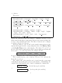
MESAFace user Manual
M. Giannotti∗, M. Wise, A. Mohammed
Barry University, 11300 NE 2nd Ave., Miami Shores, FL 33161, US
Abstract
We describe in detail how to use and customize MESAFace.
Keywords: Stellar evolution; MESA; Mathematica; GUI;
PROGRAM SUMMARY/NEW VERSION PROGRAM SUMMARY
Manuscript Title: MESAFace, a graphical interface to analyze the MESA output
Authors: M. Giannotti, M. Wise, A. Mohammed
Program Title: MESAFace
Journal Reference:
Catalogue identifier:
Licensing provisions: none
Programming language: Mathematica
Computer: Any computer capable of running Mathematica.
Operating system: Any capable of running Mathematica. Tested on Linux, Mac,
Windows XP, Windows 7.
RAM: Recommended 2 Gigabytes or more.
Number of processors used:
Supplementary material:
Keywords: Stellar evolution, MESA, Mathematica, GUI.
Classification: 1.7 Stars and Stellar Systems, 14 Graphics
External routines/libraries:
Subprograms used:
Catalogue identifier of previous version:*
Journal reference of previous version:*
Does the new version supersede the previous version?:*
Nature of problem:
∗
Corresponding author.
E-mail address: [email protected]
Preprint submitted to Computer Physics Communications
August 28, 2012
Find a way to quickly and thoroughly analyze the output of a MESA run, including
all the profiles, and have an efficient method to produce graphical representations
of the data.
Solution method:
We created two scripts (to be run consecutively). The first one downloads all the
data from a MESA run and organizes the profiles in order of age. All the files
are saved as tables or arrays of tables which can then be accessed very quickly by
Mathematica. The second script uses the Manipulate function to create a graphical interface which allows the user to choose what to plot from a set of menus and
buttons. The information shown is updated in real time. The user can access very
quickly all the data from the run under examination and visualize it with plots
and tables.
Unusual features:
Moving the slides in certain regions may cause an error message. This happens
when Mathematica is asked to read nonexistent data. The error message, however,
disappears when the slides are moved back. This issue does not preclude the good
functioning of the interface.
Additional comments:
The program uses the dynamical capabilities of Mathematica. When the program
is opened, Mathematica prompts the user to ”Enable Dynamics”. It is necessary
to accept before proceeding.
Running time:
Depends on the size of the data downloaded, on where the data are stored (harddrive or web), and on the speed of the computer or network connection. In general,
downloading the data may take from a minute to several minutes. Loading directly
from the web is slower. For example, downloading a 200MB data folder (a total of
102 files) with a dual-core Intel laptop, P8700, 2 GB of RAM, at 2.53 GHz took
about a minute from the hard-drive and about 23 minutes from the web (with a
basic home wireless connection).
1. Introduction
MESAFace is a graphical and dynamical interface to study the MESA
output. MESA (Modules for Experiments in Stellar Astrophysics) [1] is a
public available code for stellar evolution and can be downloaded at the
MESA home page [2].
MESAFace is designed to analyze the output files from a MESA run. It
is not a code for stellar evolution per-se. Some samples of output data from a
MESA run can be found on-line and can be directly accessed by the interface,
2
without the need of the MESA code. More samples of standard runs will be
added in the future and can be considered by users who are interested only in
the analysis of some standard stellar models. However, MESA is necessary
for users who want to run their own models and then analyze them with
MESAFace.
The code is written in Mathematica [3], a widely used software for graphics and mathematics. It is however, not necessary to know Mathematica to
use this interface.
MESAFace consists of two scripts, denoted by (* SCRIPT 1 *) and (*
SCRIPT 2 *), which should be run consecutively. The first downloads all the
data from a MESA run and the second creates the dynamical interface.
In this note, we will describe how to use and how to customize MESAFace.
We will assume no knowledge of Mathematica. As for the style, we will
use the Typewriter style for the content of the Mathematica notebook,
quotes for the name of the ”MESA files”, and bold face of the name of
controls in the interface.
2. Basic use of MESAFace
MESAFace uses some dynamical properties of Mathematica. Therefore,
when the MESAFace notebook is opened, Mathematica prompts a request
to enable dynamics. It is necessary to agree to that before running the
MESAFace scripts.
MESAFace needs to access the data from a MESA run. These should
be located in a folder on the hard drive or on the web. The variable path,
defined at the beginning of the first script, should point to that folder.
The first step to use MESAFace is therefore to set path. For example,
suppose the results are in the folder ”Users/mesa/OneSolarMassTest”. The
variable path should be set equal to
path="C:\\Users\\mesa\\OneSolarMassTest”;
on a windows system, and
path="C:/Users/mesa/OneSolarMassTest”;
on a Unix or Mac system. It is possible to enter the path by selecting
Insert/File Path from the Mathematica menu and navigate. In this case,
3
select any file in the data folder and then remove the name of the particular
file selected and leave only the path to the folder.
In general, path can also point to an URL (see section 4) but it cannot,
at least in the present version, download compressed files.
Next, it is necessary to run the first script (press SHIFT ENTER from
any line within the script). Mathematica will start downloading the files.
The process may take a few minutes, depending on the size of the folder and
on the speed of the computer. The progress is indicated: a numerical value
represents the actual number of downloaded files while a progress-bar shows
the relative progress.
After the files are downloaded, it is possible to run the second script,
which creates the graphical interface. This shows the controls, for example
buttons and menus, on the left side and the information, for example graphs
and tables, on the right side. Both sections are organized vertically in three
panels:
1. History;
2. Profile;
3. Info;
For definition of units of the variables used in both the history and profile
plots, and in the information panel, the user should consult the documentation on MESA.
2.1. The history plot panel
The history plot panel shows the behavior of some global star variables
at different ages. The information is extracted from the file ”star.log”. What
to plot can be decided by selecting one of the following radio buttons:
Customized, HR, CentralAbundances, Burnings.
• Customized is the default choice. In this case the variables on the x−
and y−axes can be decided from the buttons or from the pop menus.
Each pop menu contains the names of all the variables that is possible
to plot (i.e., the names of all the columns in the ”star.log” file). The
set depends on the particular run. Any of the variables in the pop
menus can be chosen to be a button for either the x− or the y−axis
(see section 3.3).
4
• HR produces the HR diagram, with the logarithm of the effective temperature on the x−axis and the logarithm of the luminosity on the
y−axis. The temperature increases toward the left of the x−axis, in
line with the standard convention for the HR diagram.
• CentralAbundances shows the central abundance of the elements defined in the list CentralAbundancesToShow in the (* General Settings
*) section of the code (see section 3.4).
• Burnings shows the energy released in the nuclear reactions defined
in the list CentralAbundancesToShow in the (* General Settings
*) section of the code (see section 3.4).
The color codes for the CentralAbundances and the Burnings options are
summarized in the help window, positioned right below the Type of Plot
menu. The number and type of elements and reactions to show, together
with the color code, can be customized, as explained in section 3.4.
The data to be shown can be manipulated from the Show menu. This
allows, for example, to take the logarithm of the data or to change sign
to the axes. The possible operations in the menu are set by the variable
DataOperations (see section 3.5).
Both axes can be scaled using the menu buttons x-axis scale and y-axis
scale. Selecting n in the x-axis scale menu rescales the x-axis by a factor
of 10−n . For example, if the x-axis represents the age in years, selecting 6 in
the x-axis scale menu would change the units to Million years. The same
for the y−axis. If a scale different from the default is chosen, its value is
indicated in the corresponding axis label.
Finally, the offset option allows to set the zero of the axes to any place.
Again, any choice different from zero is indicated in the corresponding axis
label.
In summary, the axes labels indicate the quantity being plotted, the offset
value (if different from zero) and the axes scales (if different from 1).
The slide-bars Start data point and End data point can be used to
plot only a region of the plot. They can, therefore, be used to zoom in a
particular region of the graph.
2.2. The profile plot panel
The profile plot panel shows the profiles of the star at fixed ages. The
profile plots are graphical representations of the various ”logn.data” files (n
5
is an integer). What to plot can be decided by selecting one of the following
radio buttons:
Custom, Abundances, Reactions.
• Custom is the default choice and works in the same way as for the
history plots.
• Abundances shows the profile of the abundance of the elements defined in the list ProfileAbundancesToShow in the (* General Settings
*) section of the code (see section 3.4).
• Reactions shows the energy released in the nuclear reactions defined
in the list ProfileBurningsToShow in the (* General Settings *)
section of the code (see section 3.4).
The color codes for the Abundances and the Reactions options are summarized in the help window, positioned right below the Type of Plot menu.
The number and type of elements and reactions to show, together with the
color code, can be customized, as explained in section 3.4.
The age bar is, arguably, the most prominent feature of the interface. It
allows to scroll the profiles by age rather then by number. The age change
can be animated (at different speeds) by opening the slide-bar menu (click
the sign at the end of the age slide).
If the box ”Show Age in History Plot” is checked, the age corresponding
to the current profile is shown in the history plots, therefore producing a
connection between history and profiles. The age is shown through a line,
when the x−axis is set to star age, or a dot in the other cases.
Notice, however, that there are more points in the history plot (i.e., more
lines in the ”star.log” file) than ”logn.data” files. Therefore, it is not possible,
in general, to associate a profile to each point in the history plot.
The slide-bars Start data point and End data point is used to zoom
in a particular region of the graph.
2.3. The information panel
Finally, the General Info section, represented in the last panel, shows
information on the star.
1. PATH shows the value of the variable path and so indicates the working folder or the web location from where Mathematica is extracting
the data.
6
2. GENERAL shows general information about the star not related to
the current profile. The information is taken from the second and third
rows of the file ”star.log”.
3. DETAILED shows detailed information about the current profile.
The information is taken from the second and third rows of the current
”logn.data” file.
When the DETAILED option is chosen, the information is dynamically
updated every time the age of the star is changed. This may result is a slower
and less fluid performance of MESAFace. The same is true if MESAFace is
asked to show the age in the history plot (that is, if Show Age in History
Plot is checked).
In general all the information (graphs and data) is processed only when
shown. Therefore, the less information is shown the faster and more fluid
the interface.
2.4. Saving and manipulating the graphs
Once a graph has been created, the user can utilize the Mathematica’s
functions and tools to save or to manipulate it.
To save the graph, select it (left-click on it), open the Mathematica file
menu (at the top left corner of the Mathematica window) and choose the
option save selection as. Mathematica allows the graphs to be saved in
many different formats including EPS and PDF. The plots can also be copied
to other cells to be (non-dynamically) viewed later.
The figures can also be manipulated. To do that, right-click on the figure
and select Drawing Tools from the menu. The Drawing Tools window
allows to add text and graphical objects (lines, arrows, etc.) to the graph.
Each tool has a short explanation. To read that, move the mouse on the tool
(without clicking) and wait for about a second. A noteworthy tool, which
looks like a large plus sign with dashed lines, allows to read the coordinates
of the mouse position on the graph. This can be very useful to find the exact
coordinates of a point in a plot.
3. Customization of the interface
MESAFace can be easily customized by manipulating the section contained within the comment lines
(* General Settings *)
7
and
(* DON’T CHANGE *)
at the beginning of the second script. It is not necessary to run the first
script again to update the changes in the interface.
3.1. Style of the graphs
The style of the graphs can be customized in the section (*Graphs
colors *) at the beginning of the second script. The variables HistoryGraphStyle,
ProfileGraphStyle, and AgeLineColor refer, respectively, to the style of
the history plot, the profile plots and the age line (see below). By default
the graphs are continuous. To define a dashed style, substitute Dashing[{}]
with Dashing[{r1 , r2 , ...}] where ri indicates the length of the successive
segments (repeated cyclically).
3.2. Labels
The style for the labels of the plots is set in the section (* Labels *) of
the script. The list labelsStyle defines the style of the labels of the x− and
y− axes and frameStyle refers to the style of the ticks and the tick numbers
on the axes.
In addition, both the History and Profile graphs produced by MESAFace
have, by default, a label on top which indicates the mass and metallicity of
the star for the history plots and profile number and age for the profile plots.
These labels are set by the variables HistoryPlotLabel and ProfilePlotLabel.
The second one is defined after the manipulate command and right before the (* Plot and Info Section*) of the code. Changing the value
of HistoryPlotLabel to an empty string
HistoryPlotLabel = "";
would remove the label on top of the history plot graphs. Analogously,
changing the value of PrifilePlotLabel to an empty string would remove
the label on top of the profile plot graphs.
8
3.3. Buttons
The section
(*Buttons to show*)
HistoryButtonsX = {"star age", "log Teff", "log L", "log R",
"log center T", "log center Rho"};
HistoryButtonsY = {"log Teff", "log L", "log R", "log center T",
"log center Rho"};
HistoryButtonsY2 = {"log center P", "center h1", "center he4",
"center c12"};
ProfileButtonsX = {"mass", "radius", "logR"};
ProfileButtonsY = {"radius", "mass", "logR", "logT", "logRho",
"logP", "h1", "he3", "he4"};
ProfileButtonsY2 = {"c12", "n14", "o16", "log opacity",
"luminosity", "non nuc neu"};
includes the buttons present in the interface. MESAFace allows to access
all the variables through a popup menu. However, the buttons facilitate the
access to some variables used often. The lists of buttons can be changed
according to the needs of the user.
The labels ”History” and ”Profile” in the variable names indicate if the
buttons which appear in the corresponding list refer to the History Plots
or the Profile Plots section of the interface. The labels ”X” and ”Y” at
the end of the variable names indicate if the buttons which appear in the list
refer to the x− or y−axis respectively. For example, the line
ProfileButtonsX = {"mass", "radius", "logR"};
shows the buttons for the x−axis in the profile-plot control section.
The y−variable has two rows of buttons. The label ”Y2” indicates the
list for the second row.
The complete list of the variables can be found from the popup menu
of the history and profile plots section of the interface. Alternatively, the
complete list of the variables can be found by running the command line
star[[6, All]]
(for the history plot variables),
or
log[1][[6, All]]
(for the profile plot variables),
9
in a new cell of a Mathematica notebook, after (* Script 1 *) has been
run.
3.4. Abundances and reactions to show
The section (*Abundances and Reactions to show*) contains the list
of the elements and reaction names which will be shown in the abundances
and reactions plots. The list has the form:
{ { "name 1",{ style}, "name 2",{ style}, ...
} }
and can be modified to show more or less elements or to change the style.
3.5. Units and operations on the data
The list of scaling factors defined by the control variables Cx, Cy, Dx, and
Dy described before, is set in the variable Units in the section (* Definition
of Units *) of the second script
(* Definition of Units *)
units = {{-9, " [Units: nano]"}, {-6, " [Units: micro]"},
{−3, "[Units: milli]"}, {0, ""}, {3, " [Units: kilo]"},
{6, " [Units: Mega]"}, {9, " [Units: Giga]"}};
Each entry of the list units indicates a numerical value and the corresponding
string that appears in the plot label when the scaling factor is chosen. As
explained above, selecting n for the numerical value rescales the data on the
corresponding axis by a factor of 10−n .
The list of possible functions that apply to the data is specified in the
section
(* Operations on the data*)
DataOperations = {{"",Identity[#]&},{"-",-Identity[#]&},
{"log",Log[10,#]&},{"-log",-Log[10,#]&},{"10^",10# &},
{"-10^",-10# &};
Each element of the list contains a ”string” and an ”expression”. The ”string”
represents what appears in the menu show of the interface while the ”expression” represents the actual operation to be performed on the data. The
list of functions can be changed.
10
4. Downloading directly from the web
MESAFace can download the data directly from the web. To do that,
path should point to the URL with the data folder. For example,
path=http://www.weezilla.com/M5.5 premainseq to endHeBurn
would download the data from the (existing) folder ”M5.5 premainseq to endHeBurn”,
which has the MESA results from the run of a 5.5 solar masses star, with
solar metallicity, from premainsequence till the end of the central He-burning
stage. More folders will be added in the future.
To use the web with a Windows system, however, the string slash in (*
SCRIPT 1 *) has to be changed to /. This can also be done by adding the
line
slash = "/";
to the code, just below the previous definition of slash. The line can be
removed to go back to downloading from the hard-drive. For Unix or Mac
system, it is not necessary to make any change.
Notice that downloading from the web is normally much slower than
downloading from the hard-drive.
References
[1] B. Paxton, L. Bildsten, A. Dotter, F. Herwig, P. Lesaffre and F. Timmes,
Astrophys. J. Suppl. 192, 3 (2011) [arXiv:1009.1622 [astro-ph.SR]].
[2] To download MESA and
http://mesa.sourceforge.net/
for
instructions
[3] see http://www.wolfram.com/mathematica/
11
on
its
use,
visit