Download paper - ENAC

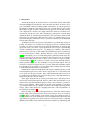
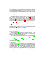
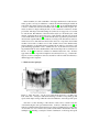
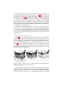
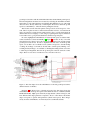
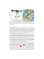
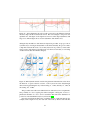
Wind parameters extraction from aircraft trajectories
C. Hurtera,∗, R. Alligiera,b , D. Gianazzaa,b , S. Puechmorela , G. Andrienkoc ,
N. Andrienkoc,d
a ENAC,
MAIAA, F-31055 Toulouse, France
de Recherche en Informatique de Toulouse, France
c Fraunhofer Institute IAIS (Intelligent Analysis and Information Systems), Sankt Augustin, Germany
d City University, London
b Institut
Abstract
When supervising aircraft, air traffic controllers need to know the current wind
magnitude and direction since they impact every flying vessel. The wind may accelerate or slow down an aircraft, depending on its relative direction to the wind. Considering several aircraft flying in the same geographical area, one can observe how the
ground speed depends on the direction followed by the aircraft. If a sufficient amount
of trajectory data is available, approximately sinusoidal shapes emerge when plotting
the ground speeds. These patterns characterize the wind in the observed area. After
visualizing this phenomenon on recorded radar data, we propose an analytical method
based on a least squares approximation to retrieve the wind direction and magnitude
from the trajectories of several aircraft flying in different directions. After some preliminary tests for which the use of the algorigthm is discussed, we propose an interactive
procedure to extract the wind from trajectory data. In this procedure, a human operator
selects appropriate subsets of radar data, performs automatic and/or manual curve fitting to extract the wind, and validates the resulting wind estimates. The operators can
also assess the wind stability in time, and validate or invalidate their previous choices
concerning the time interval used to filter the input data.
The wind resulting from the least squares approximation is compared with two
other sources – the wind data provided by Météo-France and the wind computed from
on-board aircraft parameters – showing the good performance of our algorithm. The
interactive procedure received positive feedback from air traffic controllers, which is
reported in this paper.
Keywords: Wind extraction, least squares approximation, air traffic control, data
exploration, visual analytics.
∗ Principal
Corresponding Author
Email addresses: [email protected] (C. Hurter), [email protected]
(R. Alligier), [email protected] (D. Gianazza), [email protected]
(S. Puechmorel), [email protected] (G. Andrienko),
[email protected] (N. Andrienko)
Preprint submitted to Elsevier
January 22, 2014
1. Introduction
Aircraft fly through the air, and the air flows over the Earth’s surface. This simple
statement highlights the crucial need to know the winds aloft when one wants to navigate over the Earth’s surface in a flying machine. Alternatively, one can also guess how
the wind flows simply by observing the trajectories of aircraft relative to the ground.
Interestingly enough, air traffic controllers already apply this idea in their everyday
work. Experienced controllers can roughly estimate the wind force and direction by
observing the aircraft trajectories, and comparing the ground speeds of aircraft flying
in different directions: aircraft facing the wind have a lower ground speed than aircraft
flying in the opposite direction. This basic idea is at the core of the interactive process
proposed in this paper, which allows users to extract the wind direction and magnitude
from aircraft radar tracks.
Air Traffic Controllers need accurate wind parameters to perform their activity efficiently. For instance, one can reduce the converging speed of two conflicting aircraft
by turning one aircraft so that it will face the wind. The wind impact on aircraft ground
speed is also used to slow down or speed up aircraft in order to respect a paced landing
sequence, optimizing runway usage (i.e. one landing every 3 minutes). The wind parameters are also necessary to make reliable short/medium term trajectory predictions,
so as to avoid trajectory conflicts. With the emergence of new operational concepts
[1, 2] and automated tools for air traffic management, predicting aircraft trajectories
with great accuracy has become more and more critical in recent years. For example,
medium-term conflict detection and resolution is very sensitive to trajectory prediction uncertainties [3]. In this context, it is crucial to forecast the wind with accuracy
within a prediction window of 15 to 30 minutes, at any point in the airspace. The current meteorological forecasting models do not operate within such timeframes and the
best alternative is most probably to use the current wind, assuming that it will remain
constant during the time interval of the prediction.
Estimating the current wind numerically still remains a difficult problem, as wind
measurements through sensors such as meteorological balloons or radar wind profilers are sparse in both space and time. These wind measurements must be processed
by a numerical model and the meteorological wind, pressure, and temperature data is
updated every N hours (3 hours, usually).
In this paper, flying aircraft are used as passive wind sensors, with their positions
and velocities measured through radar detection. These radar measurements are currently used for air traffic management purposes and are easily available to ground systems, in great quantities. When plotting the ground speed magnitude as a function
of ground speed direction, for a number of aircraft, some roughly sinusoidal patterns
emerge. These visual patterns are a straightforward result of the wind influence on
aircraft trajectories (Figure 1).
In the following, we propose an analytical method to extract the wind from these
patterns, using a least squares regression. Instead of focusing on one or two aircraft as
in [4], the idea is to take advantage of the amount of data, and consider categories of
aircraft with the same speed characteristics. The wind magnitude and direction is then
approximated by applying a least squares method to selected radar tracks, considering
all flights in the vicinity of the points where the wind is estimated. A simplified ground
2
speed and wind model is used, neglecting the influence of lateral drift (the drift angle
is the angle between the longitudinal axis of an aircraft and its path relative to the
ground) on the along-track ground speed. With this approximation, which is justified
for aircraft flying at high speeds, the number of unknown variables can be considerably
reduced and the model can be linearized.
We also propose an interactive semi-automatic process, where the least squares
computation is driven by the user who selects the input data and validates the results
through a visual interface.
The remainder of the paper is organized as follows: section 2 details the related
works on trajectory exploration and wind extraction, while section 3 introduces the
principles of wind extraction from a dataset of aircraft trajectories. The dataset itself is
described in section 4. The issues that were raised during some preliminary tests of the
automatic extraction method are detailed in section 5. The interactive extraction procedure mixing the least squares algorithm and user filtering and adjustments is presented
in section 6. Section 7 shows how the wind dynamics can be extracted and displayed
in order to help the user to select time windows when filtering the data. Finally, in section 8, we visually compare our results with Météo-France data. We also discuss the
confidence intervals of the least squares method and give some numerical results on the
comparison with the Météo-France wind data and the wind computed from downlinked
aircraft data. Section 9 concludes the paper and gives some perspectives about further
improvements and possible applications of our method.
2. Related work
2.1. Trajectory exploration
The data-flow model in [5] is widely used to perform data exploration. In this
paper, we also use this data flow model to transform raw data (i.e. aircraft records) into
visualization with a sequence of transformation steps.
There is a rich bibliography on trajectory analysis in information visualization, in
particular on direct manipulation to filter and extract relevant aircraft information [6, 7],
density map computation to discover boat trajectory interactions [8], aircraft trajectory
schematization [9], trajectory bundling [10], Visual Analytics [11], knowledge discovery in databases [12, 13], geocomputations [14], moving object databases [15], and
detection of landing areas [16]. However, none of these previous works tried to extract
wind parameters from trajectories.
2.2. Wind extraction
De Haan and Stoffelen [17] show that high resolution wind and temperature observations can be obtained using on-board measurements made by aircraft and transmitted
through the data-link capabilities of the Enhanced Mode-S radars (these data will be
detailed in the following). They also show how these measurements can be used as
input to meteorological models to improve the short-term and small-scale prediction of
wind and temperature. These are significant improvements when compared with the
current weather forecasts used in Air Traffic Control (ATC), and they will probably
benefit ATC operations in the future.
3
In the meantime, it is still worthwhile to investigate whether basic radar measurements (position, velocity) are sufficient to estimate the wind. Extracting the wind from
radar tracks has already been tried in other works. In [4], an extended Kalman filter
is used to estimate the wind from simulated radar tracks. This method requires two
trajectory turns for a single cruising aircraft, or, if two aircraft are considered, one turn
per aircraft. The airspeed and the turning rate (in the air) are supposed to be constant
for each aircraft. The influence of the wind on the trajectory is modeled by the ”wind
triangle” stating that the ground speed vector of each aircraft is the sum of its airspeed
vector and the wind vector. In [18], a multi-aircraft trajectory prediction problem is addressed with sequential Monte Carlo methods, focusing on the inaccuracies related to
wind forecast errors. The wind is modeled as the sum of two components: the nominal
weather forecast and a stochastic error on this weather forecast. The dimensionality
and non-linearites of the multi-aircraft problem lead the authors to introduce a new
particle filtering algorithm in order to estimate the error on the wind forecast, discarding standard methods such as Kalman filters. The aircraft airspeeds are assumed to be
known. As in [4], the method is validated on simulated trajectories only. All these
approaches are based on specific assumptions about the trajectories (e.g. constant turning rate). As these assumptions cannot be ensured for radar-recorded air traffic data, a
different approach is required.
3. Wind extraction principle
Figure 1: right “Top view”, one day of recorded aircraft trajectories over Paris area.
Left “wind view”, scatterplot with aircraft headings, and their corresponding ground
speeds. Sinus shapes emerge which show the wind influence on aircraft ground speed.
Our idea is to take advantage of the amount of data, and to consider categories
of aircraft having the same speed characteristics. Contrary to Delahaye et al. [4], our
method is validated with real aircraft trajectories instead of simulated ones, and it relies
on more than one or two aircraft. Our system uses Information Visualization (Infovis)
techniques [5] including a scatterplot and the visualization of aircraft ground speed
4
and aircraft heading. With enough data, approximately sinusoidal shapes emerge, one
for each aircraft category (or average speed category). Figure 1-right shows recorded
aircraft trajectories in 2D with their latitude and longitude. We will refer to this view
as the “top view”. Figure 1-left shows the same dataset in a scatterplot with the Xaxis showing the aircraft direction relative to the ground, and the Y-axis showing the
aircraft ground speed. This view will be referred to as the “wind view”. The emerging
sinusoidal shape is due to the wind influence on aircraft ground speed. The sine angle
shift gives the wind direction (aircraft facing the wind have the lowest ground speed),
the amplitude of the sine curve gives the wind speed (the amplitude must be divided by
two to retrieve the actual wind speed).
Specific units are used in the Air Traffic Control (ATC) community: aircraft altitudes are given in feet (ft) or Flight Levels (FL). For example, FL350 means 35,000 feet
above isobar 1013.25 hPa. Distances are given in nautical miles (NM) with 1N M =
1852m, and speeds in Knots (Kts=NM/h). In order to assess our software with air traffic controllers, we have kept these ATC-specific units in the following, instead of using
international units.
3.1. Wind influence on aircraft velocities
Figure 1 shows a scatterplot of the aircraft velocities for one day of recorded traffic.
The direction followed by the aircraft (ground track angle) is represented on the x-axis
and the magnitude of the ground speed on the y-axis. When drawing this graph, we
used a 40% transparency setting in order to emphasize the emergence of dense areas:
pixels become visible only if many plots are drawn at the same location. As seen in
Figure 1, some approximately sinusoidal shapes, stacked one upon the other, emerge
from our scatterplot. Apart from the sinusoidal curves, this visualization also shows
vertical lines which correspond to the accumulation of pixels representing aircraft with
the same direction but different speed.
Figure 2: Wind view with one day of recorded aircraft trajectories. Data filtering to
highlight wind influence on aircraft trajectories.
The emerging sinusoidal curves give a visual clue as to how the wind globally impacts the ground speed of flying aircraft. Indeed, for each sinusoidal shape, the lateral
distance (along the x-axis) between the x-coordinate of the maximum and minimum
ground speed values is 180 degrees (i.e. aircraft facing the wind have the minimum
5
ground speed, and those with the wind behind them have the maximum ground speed).
The wind magnitude can therefore be deduced by retrieving the maximum and minimum values of each sinusoidal shape and dividing their difference by two. The wind
direction can be directly deduced by considering the direction for which the ground
speed is at a maximum (i.e. when the wind is pushing the aircraft).
The fact that several sinusoidal patterns emerge reveals several categories of aircraft. Since it is quite rare that a commercial aircraft flies in circles, one such sinusoid
cannot be caused by a single aircraft. Each pattern is due to several aircraft flying in
different directions, belonging to a same category regarding their airspeed. Therefore
it does make sense to group aircraft which have similar average airspeeds.
In order to highlight the wind influence of aircraft ground speed, we used the multivariate visualization software FromDaDy [6]. Figure 2 represents one day of recorded
aircraft trajectories; image 1 shows the aircraft heading on the X axis, and the aircraft
ground speed on the Y axis. In order to emphasize the sinus wave on aircraft ground
speed, one can filter out low altitude records (which corresponds to aircraft landing
or taking off) in image 2, and remove aircraft with a vertical speed (climbing or descending aircraft) in image 3. Low altitude or climbing/descending aircraft do not have
a stable airspeed magnitude, therefore the ground speed evolutions cannot fit a sinus
shape. These records can be considered as noise, and can be removed.
Figure 3: The sinus shapes show the wind influence on aircraft ground speed at three
different clusters of altitudes.
In Figure 3 (the filtered view of aircraft trajectories) the sinus shape shows the
wind influence on aircraft ground speed at three different clusters of altitudes (FL100,
FL200 and FL300). High speed aircraft fly at high altitude (visible in image 2) and
have different sinus shape parameters compared to the two other clusters. Each sinus
shape corresponds to specific wind parameters (direction and speed). These images
clearly show the wind influence on aircraft trajectories at different altitudes.
6
3.2. Ground speed and wind model
Now that we have seen how the wind characteristics emerge from the visualized
data, let us introduce a mathematical formulation of the wind influence on aircraft
movement. In this section, we will show that the hypothesis of a sinusoidal curve
oscillating around an average speed is not exactly true, and that it requires some simplifications and approximations in the underlying model relating the ground speed to
the wind.
Considering a flight i, let us denote Vi the ground speed along the track followed
by the aircraft, and θi the track angle counted clockwise from the north reference. Ti
will denote the true airspeed (TAS), and αi the direction towards which the aircraft
is heading, i.e. the angle between the longitudinal axis of the airframe and the North
reference. Let us denote W the wind magnitude, and φ the wind direction. In the
following, vectors will be denoted in bold font (e.g. W), whereas vector magnitudes
will be in normal font (W ).
North
North
Ground track
Figure 4: Wind and aircraft velocity. Ti , True Airspeed. Vi ground speed, θi track
angle, αi aircraft heading angle, W wind magnitude, φ wind direction.
The relationship between the true airspeed, the ground speed and the wind is illustrated in Figure 4 and simply expressed as follows, using vector notations:
Vi = Ti + W
(1)
When projecting all vectors on the along-track axis, we obtain:
Vi = Ti cos(αi − θi ) + W cos(φ − θi )
(2)
Our aim is to deduce W and φ from several measurements of (θi (t), Vi (t)) made at
different times t in a chosen time interval, using several flights i. In this work, we shall
assume that all flights belonging to a same category (i.e. similar performances for the
airframe structure and engines) fly at the same average cruising speed. Of course, there
7
will remain some disparities within a same category. Even if all aircraft had the same
cruising speed in theory, this hypothesis could only be a statistical one, as airlines may
operate their flights differently depending on their cost policies.
So, on one hand, the actual dispersion of speeds within one such aircraft category
is expected to be relatively large. On the other hand, for aircraft flying at high speeds,
the drift angle αi − θi is expected to be relatively small: for an aircraft flying at about
Ti = 450 Kts with a cross-wind of 70 Kts, the error made when considering that
cos(αi − θi ) ≈ 1 is about 1 percent of the aircraft speed.
Taking these considerations into account, the exact model of equation 2 can be
simplified by replacing Ti cos(αi − θi ) by a unique speed V̄ , for all flights i belonging
to a same category. For a flight i with a velocity Vi (t) and a track angle θi (t) measured
at time t by radar detection, we then obtain the following simplified model, considering
that W and φ remain constant over the chosen time interval:
Vi (t) = V̄ + W cos(φ − θi (t))
(3)
with V̄ ∈ {V¯k |k ∈ {1, . . . , c}} the average speed corresponding to the category of
aircraft i.
The average speed V̄ does not have to be known and can be considered as an unknown variable, like W and φ. The only pre-requisite is that every flying aircraft
must be assigned to one of the existing classes {1, . . . , c} that must be determined in
advance, considering the theoretical cruising speed of each aircraft type. These theoretical cruising speeds are the results of a model ([19]) of the airframe and engine
performances provided by the aircraft manufacturers. They are available in the Eurocontrol Base of Aircraft Data (BADA, see [20]).
The above model can be linearized by introducing two new variables WX = W cos φ
and WY = W sin φ, and considering that cos(φ−θi (t)) = cos φ cos θi (t)+sin φ sin θi (t):
Vi (t) = V̄ + WX cos θi (t) + WY sin θi (t)
(4)
As the θi (t) are numerical values obtained from our radar records, we see that
Equation 4 is linear with respect to V̄ , WX , and WY .
This simplification of the initial model drastically reduces the number of unknown
variables. With equation 2, the aircraft headings αi were unknown variables. We had
one new unknown variable for each straight trajectory segment of each aircraft. With
our approximation for the drift angle, we now have only 3 unknown variables WX ,
WY , and V̄ when considering one category of aircraft, or c + 2 unknown variables
WX , WY , V¯1 , . . . , V¯c when considering c categories.
In the following, we see how the least squares approximation method can be applied
to extract the wind from an over-determined system of equations resulting from several
measurements of (θi (t), Vi (t)) from several flights i, over a chosen time interval.
3.3. Least squares approximation of the wind
Let us now consider an airspace volume A over a time interval [t1 , t2 ], assuming
the wind remains constant within this 4D-volume. Let us consider N measurements
8
{(θj , Vj )|j ∈ {1, . . . , N }} of the track angle θi (t) and ground speed Vi (t)), made at
different times t within the interval [t1 , t2 ], measured from several flights i.
Let us start with a simple case, and imagine that all aircraft flying through A belong
to a single aicraft category of mean speed V̄ . If the quality of the available data is
sufficient, that is if we have enough data with a correct dispersion of the θj values, the
unknown variables W , φ, and V̄ can be computed from the N measurements of the
track angle and velocity, considering the N corresponding instances of equation 4.
In general, N will be much greater than the number of unknown variables, and our
model (eq. 4) will not fit the observed data exactly. Let us introduce j , the difference between the velocity Vˆj computed from the model and the observed velocity Vj .
We now have a system of equations expressing linear relationships between the three
unknown variables WX , WY , and V̄ :
j = Vj − WX cos θj − WY sin θj − V̄
j ∈ {1, . . . , N }
(5)
We can use the ordinary least squares method to determine the optimum values of
WX , WY , and V̄ minimizing the quadratic error:
E(WX , WY , V̄ ) =
N
X
j=1
2j =
N
X
(Vj − WX cosθj − WY sinθj − V̄ )2
j=1
This is done by solving the linear system involving the partial derivatives of the
error with respect to the unknown variables:
∂E(WX , WY , V̄ )
=0
∂WX
∂E(WX , WY , V̄ )
=0
∂WY
∂E(WX , WY , V̄ )
=0
∂ V̄
(6)
When the associated matrix is invertible, this system will have solution (WˆX , WˆY , V̄ˆ )
that minimizes the sum-of-squares error. This solution is meaningful when the matrix
is well-conditioned.
Finally the wind is obtained using the following equations, remembering that WX =
W cos φ and WY = W sin φ:
q
2
2
W = WˆX + WˆY
(7)
WˆY
φ = arctan2 ( W
ˆ )
X
4. Available datasets
For this study, two datasets of aircraft trajectories were available, the first one
containing one day of Mode-C multi-radar records from the Paris area (France), and
the second one containing one-day records from the experimental Mode-S radar in
Toulouse (South-West of France). The dataset details and the differences between
Mode-C and Mode-S radar data are explained in the following section. Meteorological
data including wind and temperature on a fixed-size 4D-grid have been collected from
Météo-France, for the corresponding days.
9
Figure 5: Radar data (top view, right) from Toulouse Mode-S experimental radar, and
“wind view” (left). In the wind view, records are in transparent black, and those of a
same trajectory are connected by a colored line (low altitude records are in green , high
altitude in blue).
4.1. Trajectory datasets
Aircraft positions are detected by radars dispatched all over Europe. There are two
technologies for aircraft position monitoring: primary and secondary radars. Primary
radars use an emitted beam and its corresponding reflection on the aircraft body to
compute an azimuth (radar angle) and a distance (echo response time). This kind of
radar is passive : no data communication is required between the aircraft and the ground
station. Nowadays, the use of primary radars is mostly limited to military applications,
where the aircraft are assumed to be potentially non-cooperative.
Secondary radars, widely used in Civil Aviation, emit a beam which embeds a
query and then compute an azimuth and a distance thanks to the response beam emitted by the aircraft which embeds specific data. There are different types of secondary
radars, depending on the data embedded in the aircraft response. Mode-C data contains the aircraft identity and altitude reports in 100 ft intervals. Elementary Mode-S
data contains the aircraft identity, altitude reports in 25 ft intervals, and some basic
information (flight status, equipment status). Enhanced Mode-S contains useful additional information such as the aircraft velocities (ground speed, true airspeed, indicated
airspeed, Mach number), magnetic heading, roll angle, etc.
All of our radar records were obtained from secondary radars, either from a ModeC multi-radar system located in Paris (France), or from an experimental Enhanced
Mode-S radar located in Toulouse (South-West of France). We used the Paris Mode-C
dataset in preliminary experiments (see section 5) to test the least squares approximation method presented in section 3.3. This was facilitated by the presence in this
data of some extra information – the aircraft categories relative to airspeed capabilities
and operating mode (constant calibrated airspeed, or constant Mach number) – made
available by a previous post-processing of this data. These preliminary tests showed
some of the drawbacks of the fully automatic wind extraction, and motivated the semi-
10
automatic procedure presented in section 6.1. When the Toulouse Mode-S data became
available, we decided to evaluate the interactive wind extraction procedure on this new
data, allowing us to compare the results (see section 8) with Météo-France data, and
also with a wind computed from on-board measurements of the aircraft ground speed
and true airspeed. The two trajectory datasets are detailed below.
4.1.1. Mode-C radar data, Paris area
Our Mode-C records were made over an extended area in the Northern part of
France, centered on Paris (see Figure 1). The dataset contains 3,712 trajectories composed of 571,580 points with one point every 15 seconds for each aircraft. The recorded
attributes are the location (X, Y, using a Polar Stereographic WGS84 projection centered on 47N 0E), the altitude measured by the difference of pressure with isobar
1,013.25 hPa, the ground speed and ground track angle, and a unique aircraft identifier. This unique identifier is helpful to draw lines in the visualization. Distances are
counted in nautical miles (NM), speeds in knots (Kts = NM/hour), and altitudes in feet
(ft). The angles are in degrees, counted clockwise relative to the North reference. Since
we recorded the data from Paris air traffic control center, the lines representing the aircraft trajectories (Figure 1, right) end at the border of the image which corresponds to
the limits of the multi-radar coverage of this center.
4.1.2. Mode-S radar data, Toulouse area
We also investigated a second dataset from a single radar ground station located in
Toulouse (South of France, Figure 5). We used this second dataset to validate our wind
extraction algorithm since it contains additional Mode-S data. Thanks to the wind triangle principle (see 4), we can compute the wind measured on-board the aircraft. We
use this wind computed from downlinked Mode-S data as another source of meteorological data, in addition to the reference wind provided by Météo-France presented in
the next section.
Geographically, the dataset covers a circular area of radius 170 NM (315 km) centered on Toulouse. The dataset comprises 1,917 aircraft trajectories, with 169,468 radar
reports. The average time span of a trajectory is 25 minutes, with one point every 15
seconds.
4.2. Météo-France dataset
The meteorological data provided by Météo-France is a 4D-datagrid (latitude, longitude, isobar altitude, time) containing values of temperature, wind direction and magnitude. Météo-France provided us with two different meteorological datasets corresponding to the recorded days in our two radar datasets.
The 4D-grids are slightly different for these two datasets. For the one corresponding to the Mode-C radar data, the grid at a given time and altitude is composed of 151
rows and 101 columns, and is 587 NM wide and 625 NM high. The altitude varies
from isobar 1,013.25 hPa to Flight Level 340 (34,000 feet above isobar 1,013.25 hPa),
this range being split into 10 steps. The data is given every 3 hours. The grid location
starts from the North east, and continues to the South west of France and covers the
whole country. However, in our investigation, we will only consider the area which
corresponds to our multi-radar coverage.
11
The grid corresponding to the Mode-S radar dataset is made of 42 altitude levels,
and refreshed every hour. Horizontally, the grid size is 0.1 degrees (in latitude and
longitude). The visual and numerical comparisons made in section 8 use this 4D-grid.
Note however that this precise 4D-grid is not currently available in the French air traffic
control centers: The wind data is still updated every 3 hours.
Figure 6: Wind speed data provided by Météo-France at low altitude (below FL10,
left), and high altitude (above FL340, right).
Figure 6 shows the grid of wind magnitude at low and high altitudes. We can
observe that at low altitude the wind shows boisterousness whereas the wind gradient
is smoother at high altitude. One must be aware that this wind data from Météo-France
is actually not the “true” wind experienced by flying aircraft. It is the result of a process
of data assimilation and smoothing, using observations from various sensors (sounding
balloons, wind profiling radars, etc). Collecting and smoothing this data is a relatively
long process (a cycle of several hours), so the resulting wind field may not be up-todate and accurate at the time the user will exploit it. Much can be learned, however,
from the comparison of our results with this Météo-France wind model, knowing the
amount of scientific and computational effort that is devoted to developing high-quality
meteorogical models.
5. Preliminary tests and algorithm tuning
The preliminary tests presented in this section give us some insights into the behavior of the least squares method, when it is used to extract the wind parameters from
aircraft trajectory data automatically. The potential issues are illustrated by several
examples. We introduce two quality criteria for the wind estimation. Finally, we summarize the remaining issues with the automatic extraction method, and motivate the
choices made when designing the interactive wind extraction procedures presented in
section 6.1.
The preliminary tests were run on the Paris Mode-C radar records, because this data
was readily clusterized by categories of airspeed and operating mode. This clustering
allowed us to assume that all radar records within a same category belonged to aircraft
with approximately the same average true airspeed in the cruising phase.
12
5.1. Data quality issues
Basically, wind extraction consists in retrieving the estimated wind at a requested
3D-location P (x, y, z) and at a given time t. This requires the data to be filtered in time
and space, so as to select the radar plots in the neighborhood of P (x, y, z, t). The least
squares approximation is then applied to the filtered data, as described in section 3.3.
Figure 7: Not enough data to find a suitable sinus shape.
Figure 8: Limited range distribution.
Some issues regarding the quality of the input data were encountered during the
preliminary tests, when applying this basic automatic procedure. For example, if the
filtered aircraft plots are not numerous enough, the automatic extraction can fit a sinus
shape, but the wind estimation may not be accurate (Figure 7).
Even if the number of aircraft plots is sufficient, the wind estimation can be incorrect due to a limited angle distribution (Figure 8).
Figure 9: Impossibility of finding a wind estimation due to multiple solutions.
If the aircraft record angles have a large distribution, the wind estimation can still
be erroneous due to multiple possible solutions (Figure 9).
The automatic wind regression tries to minimize the quadratic error taking into
account every aircraft record. This creates an incorrect wind estimation when a cluster
of records contains outliers. A few outliers can drastically change the wind estimation
parameters (Figure 10).
13
Correct
Incorrect
Incorrect
Correct
Figure 10: Cluster of outlier records create incorrect wind estimation.
5.2. Data quality criteria, and algorithm tuning
In order to cope with some of the issues presented in the previous section, we
designed a quality criterion combining the entropy of the ground speed directions and
a threshold on the mean-square error after regression. The entropy criterion ensures
that we have a sufficient dispersion of the ground track angles, whereas the meansquare criterion limits the dispersion of velocities around the fitted sinusoidal curve.
Good entropy is sufficient to ensure that the associated matrix is well-conditioned.
The entropy is computed as follows, considering the distribution of the ground
speed directions among n equal bins partitioning the interval [0◦ , 360◦ ]:
X
Ent = −
Pi ln Pi
(8)
i
with the convention 0 × ln0 = 0, and where Pi is the empirical probability (using
normalized histograms) that a ground speed direction falls in the ith bin. The entropy
value is maximum for uniform distribution and falls when the distribution concentrates.
Taking into account these data quality criteria, the wind extraction algorithm is the
following:
1. filter the data in time and space, in the vicinity of P (x, y, z, t),
2. assess the quality of the filtered data (entropy criterion),
3. if the entropy criterion is met, apply the ordinary least squares method described
in section 3.3 to find a suitable sinus shape,
4. assess the quality of the sinus shape fitting (mean-square error criterion).
5. if the quality criteria (i.e. entropy, and mean-square error) are not met, then
return to first step and filter data from a larger neighborhood (up to a given maximum size) of P (x, y, z) and repeat the procedure.
After several tests, we empirically defined acceptable criteria with an entropy value
above 1.7 (with 20 bins) and a mean-square error below 0.35.
5.3. Summary of our preliminary findings
During our preliminary tests, we found that the introduction of data quality criteria solved the issues illustrated in Figures 7-8, thus improving the efficiency of our
extraction method. However, other issues still remain: presence of outliers, incorrect
clustering and multiple solutions. We are convinced that the automatic procedure could
14
be improved again, for example by using robust estimation methods instead of the least
squares approximation, or by applying more efficient clustering and filtering techniques
to the input data. These improvements are left for future work.
In the current paper, we propose to leave some decisions and choices to the human
operator about the assessment of the quality of both the input data and the resulting
wind estimates. While experimenting with the automatic procedure, we noticed that
inconsistent wind estimations could often and easily be spotted by a human being, by
visually comparing the wind estimates in neighboring grid cells. In the next section, we
propose an interactive procedure combining the wind extraction algorithm with manual
data-filtering and curve adjustments.
6. Interactive wind extraction
In this section, we describe our process to extract wind direction and speed with
an interactive system. In order to extract wind parameters, the user can perform an
initial automatic process. He or she defines the number of cells to investigate, and
then launches the wind extraction. The software then clusters the aircraft positions into
3D space and time, and tries to fit a sinus shape for each cell. The entropy and error
criteria are used to automatically invalidate cells with insufficient angle repartition. The
extracted wind parameters are then displayed in small multiples with an arrow in each
cell.
Figure 11 shows a top view of the adjusted wind in several grid cells at flight level
350, and also the evolution of wind over time in one of the grid cells. We see in this
example that the wind changes orientation from North to West during the day. The
computation process lasts 2 seconds with a 4x4 grid and 150,000 records. The software provides geographical grids at 4 different altitudes (FL 250 - FL 450). The arrow
indicating the wind direction is displayed with a length proportional to the corresponding wind speed.
The user can then easily recognize inconsistent wind extraction when the direction
of arrows does not correspond to the neighboring ones. Wind cannot drastically change
direction with neighboring cells. The user can then select each cell and manually adjust
extracted wind (i.e. use direct manipulation to adjust a better sinus shape), applying
a semi-automatic procedure (see section 6.1). The user can also invalidate the cell if
there is not enough data or if a suitable sinus shape cannot be adjusted.
This data validation and adjustment is fast: a few seconds for each cell that needs
to be adjusted or invalidated. In order to check if the software and procedure are easy
enough to use, we asked an air traffic controller to adjust the extracted wind parameters. Within 2 minutes, he corrected more than 10 cells (the ones with strong wind
amplitudes and those with inconsistent wind directions).
6.1. Semi-automatic procedure
The interactive procedure allowing the user to adjust the wind in a grid cell is the
following:
(a) Filtering stage: filtering is performed in space and time. As explained in section 3.1, aircraft with a vertical speed must be removed. Since aircraft with similar
15
Figure 11: Wind parameter extraction at flight level 350 (top view). The small multiples below show the wind in one cell at incremental times (morning, mid-day, afternoon, night).
cruising performances tend to fly at similar altitudes (see section 3.1), it is not essential to cluster records by aircraft category. The radar position reports can simply
be filtered by altitude range.
(b) Data quality check: records must have various ground speed directions. An entropy
value above 1.7 with 20 angle bins validates the data quality.
(c) Sinus shape extraction: thanks to the least squares estimation, a sinus shape can be
extracted from the filtered data. If the quadratic error between the filtered data and
the estimated sinus shape is below 0.35, the extraction is valid.
(d) User adjustment stage: in order to add flexibility to our wind extraction process, the
user can manually adjust the sinus shape for the grid cells exhibiting inconsistent
wind estimations.
The following three sections describe the views available to the user when adjusting
the wind in a grid-cell, how the user interacts with the system and assesses the results
of his manual adjustment.
6.2. Visualization
Our tool displays two main plots: the “top view” and the “wind view” (Figure 12).
The top view displays trajectories with a top visualization: the X-axis shows the longitudes, the Y-axis the latitudes. We also use a color gradient to display aircraft altitude:
green shades represent low altitudes and blue shades high altitudes. The top view helps
users to observe the selected 2D volume which is used to extract wind parameters.
More filtering can be performed with range sliders (Figure 12, lower right part).
16
Figure 12: Interface layout with top view (latitude, longitude), wind view (aircraft
speed, aircraft direction) and filters with range sliders used to define the 3D temporal
volume to investigate.
The wind view displays the same trajectories as shown in the top view but with a
different scatterplot configuration. The X-axis shows the aircraft direction (0-360◦ ),
whereas the Y-axis shows the aircraft ground speed. We display transparent dots that
correspond to recorded aircraft parameters. In order to visualize whether dots belong
to the same trajectory, we connect them with a line. Since the Y-axis represents aircraft
direction, many long horizontal lines appear when aircraft direction changes around 0.
In order to remove these visual artifacts and reduce cluttering, we connect trajectory
points only if the distance between dots is lower than one third of the scatterplot width.
6.3. Interactions
In the interactive procedure described at the beginning of section 6.1, the user must
be able to:
• define the extent of spatio-temporal data to be investigated (view filtering),
• adjust a sine curve so that it best fits the filtered data, when the default curve
adjusted by the least squares algorithm seems inconsistent,
• assess the wind estimation error and, if necessary, change the spatio-temporal
data to be investigated.
Each of these steps is described in detail below.
6.3.1. View filtering
In order to extract wind parameters, the user defines the temporal bounding volume
to investigate. We use the same interaction techniques available in [6]. The user leftclicks with the mouse pointer on the top view (Figure 12) to define the center of the
selected volume and then manipulates range sliders to define the time range, the altitude
range and the latitude and longitude range (Figure 12). When manipulating range
sliders, the top and the wind view are automatically updated with the filtered aircraft
17
records. The top view displays the full dataset (to provide data context) but with the
selected aircraft shown in color, and the non-selected ones in gray (Figure 12).
6.3.2. User adjustments of the sine curve
Phase adjustment
Amplitude
adjustment
Figure 13: Using direct manipulation techniques, the user can adjust the sine wave
curve location (mouse drag), and amplitude (mouse wheel).
In the next step, the user adjusts the shape of the sine curve shown in gray so that
it best fits the visualized aircraft plots in the wind view. The shape of the sine curve is
defined by the following formula:
f (angle) = Amplitude. sin(angle + Shift)
The user can change its phase (the Shif t angle value) by dragging the sinus shape
across the wind view. The user can change the sinus curve Amplitude with the mouse
wheel. When the user changes the sine wave parameters, the view updates the corresponding estimated wind speed (Amplitude/2) and direction (Shif t). These parameters are displayed as text values; in addition an oriented arrow shows the wind direction
(Figure 13).
6.3.3. User assesment of the estimated wind
In order to assess the validity of the sine wave parameters, the user can display
two estimation error metrics (Figure 14). The system computes the distance to the sine
curve for every aircraft plot. This distance is displayed with vertical yellow lines which
start from the middle of the sine wave and whose length is proportional to the computed
distance. In addition, the quadratic error is displayed as a transparent red rectangle.
The user can visually assess if the sine curve fits the aircraft plots correctly by trying
to reduce the size of the transparent red rectangle (quadratic error), and by reducing the
height of the vertical yellow lines (distance to the sine curve for each aircraft record).
7. Wind dynamic
In section 6, the illustration of the interactive procedure (Fig. 11) showed the extracted wind at several time intervals. This gave us a succint view of the wind evolution
18
Figure 14: After adjustment, the yellow peaks correspond to the difference between
the sinus shape and the actual aircraft record. The red rectangles correspond to the
quadratic error. The figure on the right shows incorrect sinus shape adjustment, with
large errors. The left figure shows a better adjustment, with smaller errors.
during the day. In addition to this interactive inspection procedure, we propose a more
systematic way to investigate the dynamics of the wind. Generally, the goal is to find a
compromise between the need to use as many trajectories as possible (to ensure sufficient coverage of the 3D space) and the need to use the most recent data (to avoid using
outdated records after the wind has changed).
Figure 15: Wind dynamic extraction with a 4x4 grid at FL 350. Each time series shows
the direction or speed evolution over time. Cell 1x1 shows how the wind changed
direction and speed during the day: in the morning 50◦ , 15 Kts, mid-day 70◦ , 5 Kts, in
the evening 110◦ , 25 Kts.
The procedure starts with a user-defined division of the territory into compartments.
One possibility is to use a regular grid, either rectangular or hexagonal. A more sophisticated alternative is to use a Voronoi tessellation that reflects the distribution of
position records and minimizes trajectory distortions [21].
Next, the user divides the time range of available data into equal time intervals (for
example, with a length of 1 hr). For each cell of the territory division and each time
19
interval the automatic wind assessment procedure is applied. In the result, time series
of wind speed and direction values are produced. These time series are presented for
inspection on time graphs and maps. Figure 15-left shows the spatial distribution of
speed dynamics at flight level 350. Similarly, Figure 15-right shows the dynamics of
directions. In both maps cell 1x1 is highlighted.
We can observe in Figure 15, that the wind speed was quite stable over the whole
time period, with a monotonous change from direction 50◦ in the morning to direction
110◦ in the evening. According to Figure 15, the wind started to blow in the morning,
slowed down at mid-day, and started again in the evening. As a result, it can be recommended to apply the analytical procedures, either fully automatic or interactive, only
to the recent data.
If the amount of trajectory data is sufficient, this procedure can be applied separately for different ranges of flight levels. By inspecting outliers on the time graph, it is
possible to identify regions that require special attention. In particular, it is necessary
to apply manual curve fitting to these cells.
8. Wind extraction results
In this section, we detail our investigations to validate our wind extraction method.
We first compare our results with two other sources of meteorological data. Then, we
report informal discussions with air traffic controllers. The results presented here were
obtained with the second dataset (Mode-S radar data, South-West of France), which
contains additional data that can be used to validate our wind extraction, in addition to
the Météo-France data.
8.1. Visual comparison with Météo-France data
Figure 16: Visual conventions for the display of speed or angle differences.
In order to ease parameter comparisons, we used two different designs to compare
wind speeds and directions. Both designs use a color gradient (green to red) to show the
error magnitude (Figure 16). In addition, the “speed” design uses a vertical line whose
length corresponds to the difference in wind magnitude between our approximation and
the Météo-France data. The “angle” design uses two lines: The white line shows the
wind direction approximated by our method, whereas the gray line shows the direction
of the Météo-France wind.
Figure 17 shows the differences between the approximated wind and the reference
wind provided by Météo-France, at various altitudes and for three different grid sizes.
The three grids at the top of Figure 17 display the automatic wind estimation, without
20
Figure 17: Wind parameter extraction and comparison with Météo-France data, with
three different grid sizes. Image 1 illustrates a manual user adjustment. Image 2 shows
an invalidated cell. Image 3 shows a valid wind extraction.
21
user adjustment. Image 1, below these three grids, shows how the user can adjust the
sinus shape to better fit the points, and ignore many outliers. Image 2 shows a cell with
a low entropy criteria (not enough data). Image 3 shows a perfect match between the
extracted wind parameters and the meteorological data.
We can see that the best results are obtained for the altitudes ranging from flight
level 300 to flight level 400. There are much fewer valid cells at very high (above flight
level 400) and very low altitudes (below flight level 300), and a few of the remaining
valid cells show marked differences with the Météo-France wind. Investigating our
dataset, we observed that very high altitudes do not contain enough data to produce
accurate wind estimations. Furthermore, at low altitudes, most aircraft are climbing or
descending and there are few trajectories at a cruising altitude with a stable airspeed.
As the records have been filtered so as to remove climbing or descending aircraft, low
altitude cells do not contain enough leveled trajectories, with a sufficient variety of
ground speed directions.
Comparing the results for wind magnitude (“speed”) and wind direction (“angle”)
in Figure 17, we can observe that the displayed error (in percentage) is smaller in
direction than in magnitude, whatever the altitude.
From this visual comparison, we can conclude that our wind approximation is closest to Météo-France data in the grid cells and at altitudes where there are many aircraft
flying in different directions, at their cruising flight level, with a stable airspeed. This
was to be expected, considering that the quality of the least squares approximation
depends on the quality of the input data.
8.2. Numerical comparison with Météo-France and Mode-S winds
Let us now present some numerical results, comparing three different wind values:
the wind approximated with the least squares method, the Météo-France wind, and a
wind computed from the ground speed and the true airspeed downlinked from the aircraft, and available in the Mode-S data provided by the experimental radar in Toulouse
(France). These three different wind values are denoted LS, MTO, and Mode-S, respectively.
100
●
●
●
LS/MTO
●
LS/Mode−S
Mode−S/MTO
(a) Wind mag. deviations
(in Kts)
0
−50
−100
●
●
−100
●
●
●
Wind direction error (deg)
−10
0
10
●
●
−150
●
50
20
●
●
●
−20
Wind magnitude error (Kts)
●
●
0
●
−50
●
Relative wind magnitude error (p.c.)
30
●
LS/MTO
LS/Mode−S
Mode−S/MTO
(b) Wind mag. deviations
(in p.c.)
●
●
LS/MTO
LS/Mode−S
Mode−S/MTO
(c) Wind dir. deviations
(in deg.)
Figure 18: Boxplots of wind deviations – in magnitude (left and middle) and direction
(right) – for all flight levels, with a 4x4 grid and a time window of 3h.
22
10
10
Figure 18 shows boxplots1 of the differences in wind magnitude – in Knots (left)
or in percentage of the reference wind (middle) – and wind direction (right) obtained
when comparing the three different wind values (LS, MTO, and Mode-S) pairwise.
The results in Figure 18 were obtained considering all flight levels, with a 4x4 grid and
a time window of 3 hours.
Considering this pairwise comparison of the three different sources, we can see
that they all provide consistent wind values. In Figure 18, the difference between the
LS approximated wind and the wind obtained from the two other sources (MTO and
Mode-S) is higher than the difference between the wind computed from Mode-S data
and the Météo-France wind. This is because Figure 18 shows the results for all flight
levels, including the LS wind estimates obtained with low quality input data.
●
●
LS/Mode−S
5
0
−5
−10
Wind magnitude error (Kts)
−20
LS/MTO
Mode−S/MTO
●
●
LS/MTO
LS/Mode−S
Mode−S/MTO
10
5
0
−5
−10
Wind magnitude error (Kts)
●
●
−15
5
0
−5
−10
Wind magnitude error (Kts)
●
(b) 1 hour time window
10
(a) 30 minute time window
−15
●
−15
5
0
−15
−10
−5
●
−20
Wind magnitude error (Kts)
●
LS/Mode−S
−20
−20
●
LS/MTO
Mode−S/MTO
(c) 2 hour time window
LS/MTO
LS/Mode−S
Mode−S/MTO
(d) 3 hour time window
Figure 19: Boxplots of wind magnitude errors (in Kts), for a 4x4 grid, at flight level
350.
Of course, results are better when focusing on flight levels where the input data is
of sufficient quality. In practice, the quality of the input data depend on several factors:
the altitude range and geographic location, and also the time window chosen when
filtering the data. Let us now focus on the upper airspace, at flight levels ranging from
1 These boxplots were obtained using the boxplot function of the R environment for statistical computing, with its default settings. The box itself represents the interquartile interval, the bold line is the median,
and the whiskers represent either an extremum value or at most 1.5 times the interquartile distance.
23
50
100
●
0
●
●
●
●
●
LS/MTO
LS/Mode−S
−100
LS/MTO
LS/Mode−S
Mode−S/MTO
Mode−S/MTO
●
LS/MTO
LS/Mode−S
−100
●
50
0
●
−100
−50
0
●
−50
50
Relative wind magnitude error (p.c.)
100
(b) 1 hour time window
100
(a) 30 minute time window
Relative wind magnitude error (p.c.)
●
−50
Relative wind magnitude error (p.c.)
50
0
−50
●
−100
Relative wind magnitude error (p.c.)
100
350 to 400, and consider the use of several time windows for the estimation of the wind
at a given time (16h, as in Figure 18). Figures 19 and 20 show the wind deviations in
magnitude, for the chosen altitude range (FL 350 to 400) and for several time windows
(30mn, 1h, 2h, 3h). Figure 21 shows the deviations in wind direction.
Mode−S/MTO
LS/MTO
(c) 2 hour time window
LS/Mode−S
Mode−S/MTO
(d) 3 hour time window
Figure 20: Boxplots of relative wind magnitude deviations (in p.c.), for a 4x4 grid, at
flight level 350.
Considering sub-figures 19d, 20d and 21d, where the time window (3 hours) is the
same as in Figure 18, we see that the differences in magnitude and direction between
the three wind values at flight levels ranging from 350 to 400 are much closer one from
the other than when considering all flight levels.
Time window size
Number of valid cells
30mn
5
1h
9
2h
13
3h
12
Table 1: Number of valid cells, using a 4x4 grid at flight levels 350-400, for time
horizons of 30mn, 1h, 2h, and 3h.
In Figures 19, 20 and 21, we can see how the choice of the time window influences
the wind estimates. Clearly, a 30-minute time window is too short. It seems that
the best results are obtained with time windows of 2 or 3 hours. However, we must be
aware that the boxplots are drawn from data of different sizes. As shown in Table 1, the
24
40
40
20
0
−20
−40
Wind direction error (deg)
−80
−60
20
0
−20
−40
−60
−80
Wind direction error (deg)
●
LS/MTO
LS/Mode−S
Mode−S/MTO
Mode−S/MTO
40
20
0
−20
−40
Wind direction error (deg)
●
●
−80
−60
20
0
−20
−40
−60
−80
Wind direction error (deg)
●
LS/Mode−S
(b) 1 hour time window
40
(a) 30 minute time window
●
LS/MTO
LS/MTO
LS/Mode−S
Mode−S/MTO
LS/MTO
(c) 2 hour time window
LS/Mode−S
Mode−S/MTO
(d) 3 hour time window
Figure 21: Boxplots of wind direction errors, for a 4x4 grid, at flight level 350.
number of valid cells (i.e. those satisfying our quality criteria) is smaller for the shortest
time windows. This should mitigate the statistical interpretation of the boxplots, and
expecially concerning the 1h-time-window, where the apparent bias towards higher
values for the deviations of the wind direction might be explained by the small sample
size. Actually, a time window of 1 to 2 hours size might be the best compromise if we
want the estimates to be sufficiently up-to-date.
The results for altitudes ranging from flight level 300 to 350 are similar to the ones
presented here (FL350-400). All these numerical results confirm the conclusion of the
visual comparison made in section 8.1. They show the good performances of the proposed wind approximation method when the input data is of sufficient quantity and
quality. In practice, the domain of application of our method is the upper airspace, at
altitudes ranging from flight level 300 to 400, with relatively dense traffic flying in various directions. At these altitudes, we find commercial aircraft of similar performances,
flying at their cruising flight level at approximately the same true airspeed.
8.3. Confidence intervals and significance testing
The numerical comparisons in the previous section are relevant only if the confidence intervals associated to the least squares estimations of the wind are of a smaller
order of magnitude than the differences with the two other winds (MTO and ModeS). Assuming we had a very large confidence interval around the wind estimate, and
25
assuming that the the Météo-France and Mode-S wind values fall within this interval,
the wind estimates and the differences between the three wind values observed in the
previous section would lose their significance.
Let us check the size of the confidence intervals associated with the least squares
approximation. In the application described in the paper, a QR decomposition of the
design matrix is preferred to the classic normal equations, trading computational efficiency for numerical stability. One benefit of the QR solution is the ease of computation of the terms involved in theexpression of the test statistics.
Denoting w̃ = Wx , Wy , V the vector of unknowns, for each of the components
w̃i , i = 1 . . . 3, of w̃, a confidence interval at level α is given by:
q
q
−3
t Z)−1 , w̃ + tN −3 e (Z t Z)−1 ]
[w̃i − tN
e
(Z
(9)
i
ii
ii
α/2
α/2
N −3
where Z is the design matrix and tα/2
is the value of the student test statistics for
confidence level α/2 and N − 3 degrees of freedom.
0.7
Size of confidence intervals
Size of confidence intervals
Avg. true airspeed estimate
0.6
Deg.
0.0
0.0
0.1
0.2
0.4
0.4
0.2
0.3
Kts
0.5
0.6
0.8
Wx
Wy
0x1 0x2 0x3 1x0 1x1 1x2 1x3 2x1 2x2 2x3 3x1 3x2 3x3
0x1 0x2 0x3 1x0 1x1 1x2 1x3 2x1 2x2 2x3 3x1 3x2 3x3
Grid cells
Grid cells
Figure 22: Size of the confidence intervals for the estimated wind (left) and for the
estimated average true airspeed, for a 4x4 grid, at flight level 350.
On the data available for the study, a very good adequation between the size of the
confidence interval and the quality of the sample assessed using the entropy criterion
was observed. Figure 22 shows the size of the confidence interval for each cell of a
4x4 grid, for (Wx , Wy ) (left) and V (right), in Kts, for altitudes ranging from flight
level 350 to 400. We see that the order of magnitude of these confidence intervals
is much smaller than the difference between the estimated wind (LS) and the other
winds (MTO and Mode-S), which comforts our analysis of the results presented in the
previous section.
26
8.4. Air traffic controllers’ feedback
In order to assess the potential operational interest of our wind extraction process,
we conducted informal discussions with air traffic controllers from Aix ATCC2 . Our
goal was to assess the validity of our wind extraction process and to understand how
air traffic controllers use wind parameters in their aircraft monitoring tasks.
We performed three interviews. Firstly we asked a set of simple questions:
• “How is the wind important in your daily work activity?”
• “How do you retrieve wind parameters?”
• “How often do you verify wind parameters?”
Secondly, we gave a software demonstration and thirdly we explained our algorithm’s rationale.
During the interview, all the controllers confirmed that wind parameters are important to their daily activity, but when we asked them how they retrieved these parameters,
their response was not unanimous. They often estimate wind parameters only by looking at the aircraft behavior. “When I compare how aircraft turn when facing north
or south, I can assess the wind direction and the wind speed”. This estimation is not
accurate but sufficient to assess approximate wind parameters. Controllers also have
a screen which displays estimated wind parameters provided by Météo-France. This
data is displayed in 2 tables with four geographically specific points each: South points
(Barcelona, Montpellier, Nice, Ajaccio) and North points (C. Ferrand, Dijon, Lyon,
Geneva) with 5 Flight Levels (180-390). These tables are updated every 3 to 6 hours.
The controllers confirmed the validity and interest of our wind parameter extraction
method. They also explained that our tool is not designed for air traffic controllers who
monitor aircraft but rather for the regulator controller, the one that supervises the traffic
regulation and does not have to deal in real-time with aircraft. The regulator controller
needs to forecast traffic evolution and therefore our dynamic wind parameter extraction
could provide valuable information for this operator.
9. Conclusion
In this paper, after visualizing the sinusoidal patterns resulting from the wind influence on aircraft ground speeds, we have proposed an analytical method to extract
the wind magnitude and direction from the radar tracks of aircraft belonging to various
speed categories. A simplified model has been introduced, allowing us to drastically reduce the number of unknown variables and to apply the ordinary least squares method
to a linearized problem. The proposed simplification consists in neglecting the effects
of lateral drift on the along-track speed for aircraft flying at high speeds. As the performance disparities among flying aircraft (even within a same speed category) are of a
greater order of magnitude than the effects of the lateral drift, this approach is justified.
2 ATCC:
Air Traffic Control Center.
27
An interactive Visual Analytics system has been developed to demonstrate the results of our automatic approach on recorded radar tracks. Users can explore, validate,
or adjust the extracted wind parameters. The wind dynamics can also be extracted from
the radar tracks and displayed as time series: Knowing the trends in wind evolution can
help the operator in the choice of a time window, when filtering the data before extracting the wind. Filtering the data is a compromise between the quantity of data required
to perform the extraction, and its temporal and spatial proximity to the point where the
wind is approximated.
The extracted wind has been compared with the Météo-France wind grid, and with
the wind computed from Mode-S data (ground speed and true airspeed) downlinked
from the aircraft. For this purpose, we used a dataset of radar reports from the experimental Mode-S radar in Toulouse (France). As a result, we have shown that the
approximated wind is very close to the wind obtained from the other two sources, at
least in airspace volumes where sufficient data is available. We have also discussed the
limitations of our method: it requires enough input data, with several aircraft flying in
various directions. In addition these aircraft should fly at similar constant airspeeds.
In practice, we have shown that this occurs in the upper airspace, where commercial
aircraft with similar performances fly at similar cruising flight levels. A good compromise for the time window used to filter the input data seems to be between 1 and 2
hours.
To summarize, our wind extraction method is most efficient when applied to the
en-route airspace, at altitudes ranging from flight level 310 to 390, where the cruising commercial traffic is of highest density. Conveniently, such airspace volumes of
high traffic density are the ones where air traffic controllers most need accurate wind
estimations for their trajectory prediction purposes. Some interviews with air traffic
controllers confirmed the interest of our approach, from an operational point of view.
Concerning the perspectives of operational use, one could think of feeding the existing meteorological models with the wind approximated from radar data. In our opinion
though, this seems a less promising approach than using the aircraft on-board measurement of the true airspeed and ground speed, downlinked to ground systems via Mode-S.
However, collecting and using such data does require fully deployed Mode-S datalink
capabilities, and also some additional data processing in order to remove some equipment biases (see [17]). There are good hopes that such wind predictions with enhanced
accuracy will be made available in the future, at least in the core traffic areas where
Mode-S radars are being deployed. In the meantime, our method could be used as
an inexpensive alternative to this approach. It could provide up-to-date wind estimations in dense en-route airspace areas, as a complement to the meteorological wind grid
which is currently refreshed every hour at best3 . It could also be useful in geographic
areas not covered by accurate meteorological models, or where Mode-S capabilities
will not be deployed.
As future work, we plan to try robust estimation methods instead of the ordinary
least squares approximation. More extensive numerical experiments could also help
to tune our data quality criteria. Another promising path could be to take into account
3 For
the Rapid Refresh (RAP) in the U.S.
28
some constraints on the wind field (minimum L2 norm of the Laplacian), so as to improve our wind estimation. Concerning the interactive procedure, further investigations
are in progress, to validate the user performance when adjusting the sinus shape. Finally, we plan to design a specific system to emphasize wind dynamic perception for
the air traffic controller.
Acknowledgements
We would like to thank Christophe Baehr and Météo-France for providing the
météorological data used in this study, and the French Air Traffic Services provider
(DSNA) for making the radar records available to us. Many thanks also to Serge Roux
(ENAC) for collecting and post-processing the Mode-S radar data.
References
[1] SESAR Consortium. Milestone Deliverable D3: The ATM Target Concept. Technical report, 2007.
[2] Harry Swenson, Richard Barhydt, and Michael Landis. Next generation air transportation system (ngats) air traffic management (atm)-airspace project. Reference
Material, External Release Version, NASA, 2006.
[3] Jean-Marc Alliot, Nicolas Durand, and Géraud Granger. A statistical analysis of
the influence of vertical and ground speed errors on conflict probe. In 4th Air
Traffic Management Research & Development Seminar, Santa Fe (USA), 2001.
[4] Daniel Delahaye and Stephane Puechmorel. Tas and wind estimation from radar
data. In Digital Avionics Systems Conference, 2009. DASC ’09. IEEE/AIAA 28th,
pages 2.B.5–1–2.B.5–16, 2009.
[5] Stuart K Card, Jock D Mackinlay, and Ben Schneiderman. Readings in information visualization: using vision to think. Morgan Kaufmann, 1999.
[6] Christophe Hurter, Benjamin Tissoires, and Stéphane Conversy. Fromdady:
Spreading aircraft trajectories across views to support iterative queries. Visualization and Computer Graphics, IEEE Transactions on, 15(6):1017–1024, 2009.
[7] Christophe Hurter, Ozan Ersoy, and Alexandru Telea. Moleview: An attribute
and structure-based semantic lens for large element-based plots. Visualization
and Computer Graphics, IEEE Transactions on, 17(12):2600–2609, 2011.
[8] Roeland Scheepens, Niels Willems, Huub van de Wetering, Gennady Andrienko,
Natalia Andrienko, and Jarke J van Wijk. Composite density maps for multivariate trajectories. Visualization and Computer Graphics, IEEE Transactions on,
17(12):2518–2527, 2011.
29
[9] Christophe Hurter, Mathieu Serrurier, Roland Alonso, Gilles Tabart, and JeanLuc Vinot. An automatic generation of schematic maps to display flight routes
for air traffic controllers: structure and color optimization. In Proceedings of the
International Conference on Advanced Visual Interfaces, pages 233–240. ACM,
2010.
[10] Christophe Hurter, Ozan Ersoy, and Alexandru Telea. Smooth bundling of large
streaming and sequence graphs. 2013.
[11] Natalia Andrienko and Gennady Andrienko. Visual analytics of movement: An
overview of methods, tools and procedures. Information Visualization, 12(1):3–
24, 2013.
[12] Gianni Giannotti, Fosca Giannotti, and Dino Pedreschi. Mobility, data mining
and privacy: Geographic knowledge discovery. Springer, 2008.
[13] Gennady Andrienko and Natalia Andrienko. Visual exploration of the spatial distribution of temporal behaviors. In Information Visualisation, 2005. Proceedings.
Ninth International Conference on, pages 799–806. IEEE, 2005.
[14] Patrick Laube. Progress in movement pattern analysis. In BMI Book, pages 43–
71, 2009.
[15] Ralf Hartmut Güting and Markus Schneider. Moving objects databases. Access
Online via Elsevier, 2005.
[16] Gennady Andrienko, Natalia Andrienko, Christophe Hurter, Salvatore Rinzivillo,
and Stefan Wrobel. Scalable analysis of movement data for extracting and exploring significant places. 2012.
[17] Siebren De Haan and Ad Stoffelen. Assimilation of high-resolution Mode-S wind
and temperature observations in a regional NWP model for nowcasting applications. Weather and Forecasting, 27(4):918–937, 2012.
[18] Ioannis Lymperopoulos and John Lygeros. Sequential monte carlo methods for
multi-aircraft trajectory prediction in air traffic management. International Journal of Adaptive Control and Signal Processing, 2010.
[19] Base of aircraft data (BADA) aircraft performance modelling report. Technical
report, EUROCONTROL, 2009.
[20] Angela Nuic. User manual for base of aircarft data (bada) rev.3.9. Technical
report, EUROCONTROL, 2011.
[21] Natalia Andrienko and Gennady Andrienko. Spatial generalization and aggregation of massive movement data. Visualization and Computer Graphics, IEEE
Transactions on, 17(2):205–219, 2011.
30