Download On-line guide - Service web

User’s Guide for ContactCenters Simulation Library
Generic Simulator for Blend and Multi-skill Call Centers
Version: July 1, 2009
Eric Buist
This document introduces a generic simulator for blend and multi-skill call centers. The
simulator is written using Java, SSJ, and the ContactCenters library. It is configured using
XML files and supports call centers with inbound and outbound calls of multiple types,
multiple groups of agents, and complex routing policies. This document presents the model
implemented by the simulator, the format of the configuration files with some examples,
and instructions to run the simulator from the command-line and to extend it internally in
Java code. We also provide a reference guide documenting every supported parameter and
performance measure. In this document, any reference to a contact corresponds to a call,
since the simulator only considers calls as type of contacts.
CONTENTS i
July 1, 2009
Contents
I
Tutorial
2
1 Overview
2
2 Simulation model
4
2.1
The simulation horizon divided into periods . . . . . . . . . . . . . . . . . .
4
2.2
The processing of a call . . . . . . . . . . . . . . . . . . . . . . . . . . . . . .
5
2.2.1
Inbound calls . . . . . . . . . . . . . . . . . . . . . . . . . . . . . . .
6
2.2.2
Outbound calls . . . . . . . . . . . . . . . . . . . . . . . . . . . . . .
6
2.3
The agent groups . . . . . . . . . . . . . . . . . . . . . . . . . . . . . . . . .
7
2.4
The router . . . . . . . . . . . . . . . . . . . . . . . . . . . . . . . . . . . . .
9
2.5
Call transfers . . . . . . . . . . . . . . . . . . . . . . . . . . . . . . . . . . .
10
2.6
Virtual queueing or call backs . . . . . . . . . . . . . . . . . . . . . . . . . .
12
2.7
Simulation experiments . . . . . . . . . . . . . . . . . . . . . . . . . . . . . .
13
2.8
Simulation output . . . . . . . . . . . . . . . . . . . . . . . . . . . . . . . . .
14
2.9
The simplified CTMC model . . . . . . . . . . . . . . . . . . . . . . . . . . .
15
3 Examples of data files
17
3.1
Single queue . . . . . . . . . . . . . . . . . . . . . . . . . . . . . . . . . . . .
17
3.2
Variants of the single-queue model . . . . . . . . . . . . . . . . . . . . . . . .
23
3.2.1
Disabling abandonment
. . . . . . . . . . . . . . . . . . . . . . . . .
23
3.2.2
Setting period-specific parameters . . . . . . . . . . . . . . . . . . . .
23
3.2.3
Increasing the variability of arrivals . . . . . . . . . . . . . . . . . . .
24
3.2.4
Changing the number of periods . . . . . . . . . . . . . . . . . . . . .
24
3.2.5
Adding a new call type . . . . . . . . . . . . . . . . . . . . . . . . . .
25
3.2.6
Adding a new agent group . . . . . . . . . . . . . . . . . . . . . . . .
27
3.2.7
Adding routing delays . . . . . . . . . . . . . . . . . . . . . . . . . .
29
3.2.8
Using agent schedules . . . . . . . . . . . . . . . . . . . . . . . . . . .
30
3.2.9
Estimating parameters . . . . . . . . . . . . . . . . . . . . . . . . . .
31
Additional experiment parameters . . . . . . . . . . . . . . . . . . . . . . . .
33
3.3.1
Getting a call-by-call trace . . . . . . . . . . . . . . . . . . . . . . . .
33
3.3.2
Restricting the printed statistics . . . . . . . . . . . . . . . . . . . . .
34
3.3
ii CONTENTS
July 1, 2009
3.3.3
Printing observations . . . . . . . . . . . . . . . . . . . . . . . . . . .
34
3.3.4
Changing random seeds . . . . . . . . . . . . . . . . . . . . . . . . .
35
3.3.5
Sequential sampling . . . . . . . . . . . . . . . . . . . . . . . . . . . .
36
3.3.6
Parameters for the CTMC simulator . . . . . . . . . . . . . . . . . .
37
3.4
Stationary multi-skill call center . . . . . . . . . . . . . . . . . . . . . . . . .
37
3.5
Generalizing routing using matrices of ranks . . . . . . . . . . . . . . . . . .
40
3.6
Longest weighted waiting times . . . . . . . . . . . . . . . . . . . . . . . . .
41
3.7
The local-specialist router’s policy . . . . . . . . . . . . . . . . . . . . . . . .
45
3.8
More complex routing policies . . . . . . . . . . . . . . . . . . . . . . . . . .
52
3.8.1
A single waiting queue, two call types . . . . . . . . . . . . . . . . . .
53
3.8.2
Priorities changing with waiting time . . . . . . . . . . . . . . . . . .
55
3.8.3
Two call types and agent groups . . . . . . . . . . . . . . . . . . . . .
58
3.8.4
Simulating routing and transfer delays . . . . . . . . . . . . . . . . .
60
3.8.5
Conditional routing . . . . . . . . . . . . . . . . . . . . . . . . . . . .
62
Blend call center model . . . . . . . . . . . . . . . . . . . . . . . . . . . . . .
65
3.10 Blend and multi-skill call center . . . . . . . . . . . . . . . . . . . . . . . . .
68
3.11 Imposing limits on the number of outbound calls
. . . . . . . . . . . . . . .
72
3.12 Call transfers . . . . . . . . . . . . . . . . . . . . . . . . . . . . . . . . . . .
73
3.13 Virtual queueing . . . . . . . . . . . . . . . . . . . . . . . . . . . . . . . . .
77
3.9
4 Running simulations from the command line
4.1
81
Calling the generic simulator from the command-line . . . . . . . . . . . . .
81
4.1.1
Calling the CTMC simulator . . . . . . . . . . . . . . . . . . . . . . .
83
4.1.2
Passing options to the JVM . . . . . . . . . . . . . . . . . . . . . . .
83
Exporting the statistical report . . . . . . . . . . . . . . . . . . . . . . . . .
84
4.2.1
Case sensitivity . . . . . . . . . . . . . . . . . . . . . . . . . . . . . .
84
4.2.2
Exporting versus redirection . . . . . . . . . . . . . . . . . . . . . . .
85
4.2.3
Existing output file . . . . . . . . . . . . . . . . . . . . . . . . . . . .
85
4.3
Getting estimated parameters . . . . . . . . . . . . . . . . . . . . . . . . . .
85
4.4
Converting old parameter files . . . . . . . . . . . . . . . . . . . . . . . . . .
85
4.2
July 1, 2009
CONTENTS iii
5 Running simulations from Java code
5.1 Getting estimates for performance measures . . . . . . . . . . . . .
5.2 Exporting results . . . . . . . . . . . . . . . . . . . . . . . . . . . .
5.3 Extracting observations . . . . . . . . . . . . . . . . . . . . . . . . .
5.4 Tracking the progress of a simulation . . . . . . . . . . . . . . . . .
5.5 Running experiments with multiple staffing levels . . . . . . . . . .
5.6 Controlling the random seeds . . . . . . . . . . . . . . . . . . . . .
5.7 Extracting parameters . . . . . . . . . . . . . . . . . . . . . . . . .
5.8 Constructing parameter objects . . . . . . . . . . . . . . . . . . . .
5.9 Performing a sensitivity analysis . . . . . . . . . . . . . . . . . . . .
5.10 Performing simulations in parallel . . . . . . . . . . . . . . . . . . .
5.11 Making an histogram of the waiting time distribution . . . . . . . .
5.12 Using a custom probability distribution or random variate generator
5.13 Implementing a custom routing policy . . . . . . . . . . . . . . . .
.
.
.
.
.
.
.
.
.
.
.
.
.
.
.
.
.
.
.
.
.
.
.
.
.
.
.
.
.
.
.
.
.
.
.
.
.
.
.
.
.
.
.
.
.
.
.
.
.
.
.
.
.
.
.
.
.
.
.
.
.
.
.
.
.
6 Troubleshooting
6.1 Commands not found or NoClassDefFoundError messages . . . . . . . . . .
6.2 Unmarshalling errors . . . . . . . . . . . . . . . . . . . . . . . . . . . . . . .
6.2.1 Missing ending tag . . . . . . . . . . . . . . . . . . . . . . . . . . . .
6.2.2 Forgotten closing bracket . . . . . . . . . . . . . . . . . . . . . . . . .
6.2.3 Missing namespace URI . . . . . . . . . . . . . . . . . . . . . . . . .
6.2.4 Invalid name of attribute . . . . . . . . . . . . . . . . . . . . . . . . .
6.2.5 Invalid format for a numeric parameter . . . . . . . . . . . . . . . . .
6.2.6 Invalid name of element . . . . . . . . . . . . . . . . . . . . . . . . .
6.3 CallCenterCreationException . . . . . . . . . . . . . . . . . . . . . . . . .
6.3.1 Invalid name of probability distribution . . . . . . . . . . . . . . . . .
6.3.2 Incorrect number of parameters for a probability distribution . . . . .
6.3.3 Invalid parameters for a probability distribution . . . . . . . . . . . .
6.3.4 Not enough arrival rates . . . . . . . . . . . . . . . . . . . . . . . . .
6.3.5 Invalid dimensions of matrix of ranks . . . . . . . . . . . . . . . . . .
6.4 Execution errors . . . . . . . . . . . . . . . . . . . . . . . . . . . . . . . . . .
6.4.1 OutOfMemoryError . . . . . . . . . . . . . . . . . . . . . . . . . . . .
6.4.2 IOException . . . . . . . . . . . . . . . . . . . . . . . . . . . . . . .
6.4.3 Warnings about detailed agent groups followed by an IllegalStateException . . . . . . . . . . . . . . . . . . . . . . . . . . . . . . . . .
6.4.4 Infinite loops . . . . . . . . . . . . . . . . . . . . . . . . . . . . . . .
6.4.5 NullPointerException and other exceptions . . . . . . . . . . . . .
6.4.6 Slow simulation . . . . . . . . . . . . . . . . . . . . . . . . . . . . . .
86
86
89
90
92
94
98
101
103
106
114
118
124
125
131
131
131
131
132
133
133
134
134
135
135
136
136
137
137
138
138
139
139
139
140
140
iv CONTENTS
II
July 1, 2009
Reference documentation
141
7 Overview
141
8 The XML format used by the simulator
142
8.1
Overview of the XML format . . . . . . . . . . . . . . . . . . . . . . . . . . 142
8.2
Supported data types . . . . . . . . . . . . . . . . . . . . . . . . . . . . . . . 143
8.2.1
Simple data types . . . . . . . . . . . . . . . . . . . . . . . . . . . . . 144
8.2.2
Complex data types
. . . . . . . . . . . . . . . . . . . . . . . . . . . 145
8.3
Available arrival processes . . . . . . . . . . . . . . . . . . . . . . . . . . . . 146
8.4
Available dialer’s policies . . . . . . . . . . . . . . . . . . . . . . . . . . . . . 150
8.5
Available router’s policies . . . . . . . . . . . . . . . . . . . . . . . . . . . . 154
9 Types of experiments
165
9.1
Finite horizon . . . . . . . . . . . . . . . . . . . . . . . . . . . . . . . . . . . 165
9.2
Steady-state . . . . . . . . . . . . . . . . . . . . . . . . . . . . . . . . . . . . 166
10 The output of the simulator
169
10.1 The contents of a report . . . . . . . . . . . . . . . . . . . . . . . . . . . . . 169
10.2 The format of the report . . . . . . . . . . . . . . . . . . . . . . . . . . . . . 171
10.2.1 Program-readable format . . . . . . . . . . . . . . . . . . . . . . . . . 171
10.2.2 Plain text . . . . . . . . . . . . . . . . . . . . . . . . . . . . . . . . . 171
10.2.3 Microsoft Excel . . . . . . . . . . . . . . . . . . . . . . . . . . . . . . 172
10.2.4 Localized format for reports . . . . . . . . . . . . . . . . . . . . . . . 172
10.3 Available performance measures . . . . . . . . . . . . . . . . . . . . . . . . . 173
10.4 Supported row types . . . . . . . . . . . . . . . . . . . . . . . . . . . . . . . 192
10.5 Supported column types . . . . . . . . . . . . . . . . . . . . . . . . . . . . . 194
10.6 Supported estimation types . . . . . . . . . . . . . . . . . . . . . . . . . . . 195
July 1, 2009
LIST OF TABLES v
List of Tables
1
Parameters for the most commonly used probability distributions . . . . . .
21
2
Parameters in the Web form for CCmath with corresponding parameters in
the sim2skill.xml file . . . . . . . . . . . . . . . . . . . . . . . . . . . . . .
44
3
XML entities used to escape reserved characters . . . . . . . . . . . . . . . . 143
4
Supported symbols for time units . . . . . . . . . . . . . . . . . . . . . . . . 144
5
Most common Java properties affecting reporting . . . . . . . . . . . . . . . 172
6
Example of a matrix of performance measures . . . . . . . . . . . . . . . . . 173
vi LIST OF FIGURES
July 1, 2009
List of Figures
1
The Implemented Model of Call Center . . . . . . . . . . . . . . . . . . . . .
4
2
The simulated horizon . . . . . . . . . . . . . . . . . . . . . . . . . . . . . .
5
3
The path of a call in the call center . . . . . . . . . . . . . . . . . . . . . . .
6
4
The path of an outbound call in the call center . . . . . . . . . . . . . . . . .
8
5
The transfer of a call to a secondary agent . . . . . . . . . . . . . . . . . . .
11
6
Virtual queueing of a call . . . . . . . . . . . . . . . . . . . . . . . . . . . . .
12
7
The hierarchical structure of example in Listing 1 . . . . . . . . . . . . . . .
19
July 1, 2009
LISTINGS vii
Listings
1
2
3
4
5
6
7
8
9
10
11
12
13
singleQueue.xml: Example of a parameter file for a call center with a single
queue . . . . . . . . . . . . . . . . . . . . . . . . . . . . . . . . . . . . . . .
17
repSimParams.xml: Example of a parameter file for an experiment using
independent replications . . . . . . . . . . . . . . . . . . . . . . . . . . . . .
22
singleQueueTwoTypes.xml: Example of a parameter file for a call center with
a single agent group and two call types . . . . . . . . . . . . . . . . . . . . .
26
singleQueueTwoGroups.xml: Example of a parameter file for a call center
with two agent groups and a single call type . . . . . . . . . . . . . . . . . .
28
singleQueueShifts.xml: Example of a parameter file for a call center with
a single agent group with a schedule, and a single call type . . . . . . . . . .
30
singleQueueMLE.xml: Example of a parameter file with data for parameter
estimation . . . . . . . . . . . . . . . . . . . . . . . . . . . . . . . . . . . . .
32
repSimParamsTr.xml: Example of a parameter file for an experiment using
independent replications and producing a call-by-call trace . . . . . . . . . .
34
repSimParamsStat.xml: Example of a parameter file for an experiment using
independent replications and producing a report with selected statistics . . .
34
repSimParamsObs.xml: Example of a parameter file for an experiment using
independent replications and producing a report with selected lists of observations . . . . . . . . . . . . . . . . . . . . . . . . . . . . . . . . . . . . . . .
35
repSimParamsSeed.xml: Example of a parameter file for an experiment using
independent replications and different initial seed . . . . . . . . . . . . . . .
36
repSimParamsSeqSamp.xml: Example of a parameter file for an experiment
using independent replications and sequential sampling . . . . . . . . . . . .
36
repSimParamsCTMC.xml: Example of a parameter file for an experiment using
independent replications and CTMC simulator . . . . . . . . . . . . . . . . .
37
mskccParamsThreeTypes.xml: Example of a parameter file for a multi-skill
stationary call center . . . . . . . . . . . . . . . . . . . . . . . . . . . . . . .
37
14
batchSimParams.xml: Example of a parameter file for a stationary simulation 40
15
sim2skill.xml: Example of a parameter file for a call center with longest
weighted waiting time router . . . . . . . . . . . . . . . . . . . . . . . . . . .
42
mskccParamsThreeTypesReg.xml: Example of a parameter file for a call center with local-specialist router . . . . . . . . . . . . . . . . . . . . . . . . . .
45
Parameters for the local-specialist routing policy with type-to-group map
equivalent to example in Listing 16 . . . . . . . . . . . . . . . . . . . . . . .
50
Parameters for the agents’ preference-based routing policy with delays equivalent to local-specialist . . . . . . . . . . . . . . . . . . . . . . . . . . . . . .
51
16
17
18
July 1, 2009
LISTINGS 1
19
op-singleQueue.xml: Example of a configuration file using the OVERFLOWANDPRIORITY
routing policy giving priority to a call type over the other one . . . . . . . . 53
20
Part of op-singleQueue-cp.xml: routing parameters for an example of priorities of calls evolving with waiting time . . . . . . . . . . . . . . . . . . . .
56
21
op-twoQueues.xml: Example of a configuration file using the OVERFLOWANDPRIORITY
routing policy, with two call types and agent groups . . . . . . . . . . . . . . 58
22
Part of op-twoQueues-slowOv.xml: parameters of a routing policy including
routing delays and transfer times . . . . . . . . . . . . . . . . . . . . . . . .
61
23
Part of op-twoQueues-cond.xml: example of parameters for conditional routing 62
24
Part of op-twoQueues-condStat.xml: example of parameters for conditional
routing depending on the service level observed during the last five minutes .
64
25
mskBlendSim.xml: Example of a parameter file for a blend call center . . . .
65
26
mskInOutSim.xml: Example of a parameter file for a blend and multi-skill
call center . . . . . . . . . . . . . . . . . . . . . . . . . . . . . . . . . . . . .
68
27
Dialer producing two call types, and using limits . . . . . . . . . . . . . . . .
72
28
callTransfers.xml: Example of a parameter file for a model with call transfers 73
29
vq.xml: Example of a parameter file for a model with virtual queueing . . .
77
30
Sample output of the simulator . . . . . . . . . . . . . . . . . . . . . . . . .
81
31
CallSim.java: calling the simulator to extract the service level . . . . . . .
87
32
Part of CallSimSL.java: obtaining service level estimates for each call type
and acceptable waiting time . . . . . . . . . . . . . . . . . . . . . . . . . . .
88
33
CallSimExport.java: calling the simulator to export results . . . . . . . . .
89
34
CallSimObs.java: calling the simulator to extract observations . . . . . . .
91
35
CallSimListener.java: tracking the progress of a call center simulator . . .
92
36
CallSimSubgradient.java: estimating a subgradient . . . . . . . . . . . . .
95
37
TestCRN.java: estimating a difference with CRNs . . . . . . . . . . . . . . .
98
38
GetParams.java: getting the arrival rates, service rates, and staffing vector . 101
39
CreateParams.java: creating an instance of CallCenterParams from scratch 104
40
SimulateScenarios.java: simulating scenarios for sensitivity analysis . . . 107
41
WriteSummary.java: simple program writing summary results for different
scenarios . . . . . . . . . . . . . . . . . . . . . . . . . . . . . . . . . . . . . . 111
42
SimulateScenariosThreads.java: simulate scenarios with multiple threads
43
WaitingTimeHistogram.java: program constructing an histogram for the
waiting time distribution . . . . . . . . . . . . . . . . . . . . . . . . . . . . . 119
44
ExpKernelDensityGen.java: random variate generator using kernel density
with a Gaussian kernel . . . . . . . . . . . . . . . . . . . . . . . . . . . . . . 124
45
Sim2SkillRouter.java: simulation program using a custom router . . . . . 126
114
2 1 OVERVIEW
July 1, 2009
Part I
Tutorial
1
Overview
A contact center is a set of resources (communication equipment, employees, computers,
etc.) providing an interface between customers and a business [16, 7, 4, 1]. Each contact
represents a customer reaching the contact center to obtain some form of service. The service
is made by employees in the contact centers called agents. Each agent is a member of an agent
group which determines its characteristics (skills, speed of service, etc.). When a contact
cannot be served immediately, it is put in a waiting queue to be served later. The contact
center components are linked together by a router which decides on how to assign calls to
agents. A call center is a special form of contact center where each contact corresponds to
a telephone call.
The ContactCenters library is built using the Java programming language [8], and
Stochastic Simulation in Java (SSJ) library [14], and permits one to implement simulators for contact centers. The library provides building blocks such as classes representing
the contacts in the center, the agent groups, the waiting queues, and the router. The programmer combines these blocks to make a simulator. However, creating a simulator directly
using this library involves Java programming.
This document presents a ready-to-use generic simulator for the particular case of a blend
and multi-skill call center with multiple call types, agent groups and simulation periods. It
can simulate inbound calls arriving in the system following a stochastic arrival process as well
as outbound calls made by predictive dialers. Service and patience times are also random,
and come from any probability distribution supported by SSJ, and parameters can change
from time periods to periods.
This simulator is configured through XML files. Compilation of Java code is not required,
except if the simulator has to be extended, or used internally by another program. Any XML
document intended to be processed by a program conforms to a schema. The simulator uses
one such schema for the parameters of the simulated model, and a second schema for the
parameters of the experiment method.
The rest of this document is organized as follows. In the next section, we present the call
center model implemented by the generic simulator. We define the structure of possible call
centers as well as the supported types of experiments. Section 3 introduces the format of the
configuration files for the simulator by some commented examples. This is a good way to
learn how to make configuration files, not a reference documentation. Section 4 demonstrates
how to run the simulator from the command-line while section 5 shows how to interact with
the simulator from a Java program. Section 6 discusses most common problems encoutered
when using the simulator. The last sections contain a reference manual providing detailed
documentation for each supported performance measure, routing policies, dialing policies,
arrival processes, the supported types of experiments, and the format of generated reports.
July 1, 2009
3
Section 8 gives a primer on XML, and the data types used in the parameter files. It
also gives some examples on how parameter-specific documentation, which is available in
HTML only, can be retrieved. The documentation for each parameter was generated from
the annotations in the corresponding XML schemas, and can be located in the doc/schemas
subdirectory of ContactCenters.
4 2 SIMULATION MODEL
2
July 1, 2009
Simulation model
This section gives a description of the model implemented by the simulator, without references to specific parameter names in the XML configuration file. See the next section
for example configuration files, section 8 for a primer on XML and the data types used in
parameter files, and the HTML documentation of the XML Schemas of CotnactCenters for
more information on parameter names.
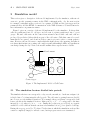
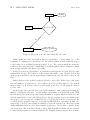
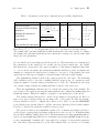
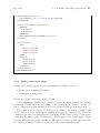
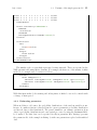
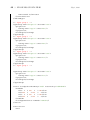
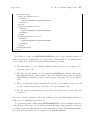
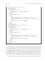
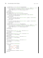
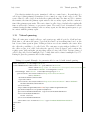
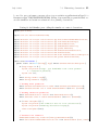
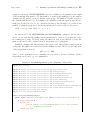
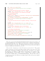
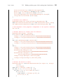
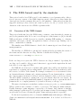
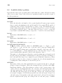
Figure 1 gives an overview of the model implemented by the simulator. It shows that
calls are partitionned into K call types and are sent to agents partitionned into I agent
groups. Inbound calls arrive in the center from external sources while outbound calls are
produced by predictive dialers which are part of the call center. Calls that cannot be served
immediately are queued, and abandon if they cannot get service after a certain patience
time. However, the model is more complex than the figure shows: the queueing discipline is
not always first-in first-out, routing can consider agents with multiple skills, and parameters
can change during the day. Next sections will examine these aspects in more details.
Abandonment
0
..
.
KI − 1
KI
1
K−1
N0 (t)
..
.
Waiting queue
..
.
...
1
...
NI−1 (t)
Agent groups
Contact types
Figure 1: The Implemented Model of Call Center
2.1
The simulation horizon divided into periods
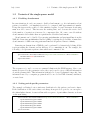
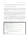
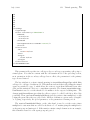
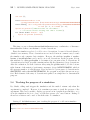
The simulation horizon can correspond to a day, a week, a month, etc. As shown on figure 2, it
is divided into P +2 time intervals called periods. The call center’s opening hours are divided
into P main periods with fixed duration d. For example, these periods may correspond to half
hours or hours in the simulated horizon. Main period p = 1, . . . , P corresponds to the time
interval [tp−1 , tp ), where 0 ≤ t0 < · · · < tP . During the preliminary period [0, t0 ), no agent is
available to serve calls but arrivals can start a few minutes before t0 for a queue to build up.
During the wrap-up period [tP , T ], where T is the time at which the simulation ends and the
center is completely empty, no arrival occurs, but in-progress services are terminated.
2.2 The processing of a call 5
July 1, 2009
Main periods
...
Preliminary
0
t0
t1
t2
Wrap-up
tP
T
Figure 2: The simulated horizon
Parameters are usually specified for the main periods only. During the preliminary period,
there are no agents to serve calls and if other parameters are needed, the simulator takes
them from the first main period. During the wrap-up period, the parameters from the last
main period are used. The preliminary and wrap-up periods can have a length of 0 in several
models. They are useful to simulate one day starting where t0 > 0. Since the preliminary
and wrap-up periods are secondary, main periods are often denoted as the periods in the
rest of this document.
2.2
The processing of a call
The set of K call types is divided into two subsets: KI ≤ K inbound call types with indices
0, . . . , KI − 1, and KO outbound call types with indices KI , . . . , K − 1. Each call type can
have its own call source which produces only calls of this type, and can be shut up and down
at any time during the simulation. In addition, call sources producing calls of multiple,
randomly-chosen types, can be defined. In the latter case, if a call is generated during main
period p, its type is k with a fixed probability pk,p , independently of other calls. The way
calls are produced depends on whether they are inbound or outbound, and will be covered
in the next subsections.
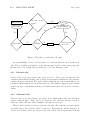
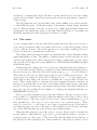
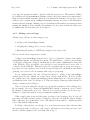
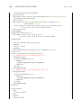
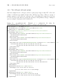
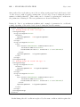
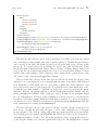
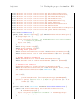
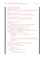
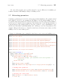
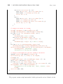
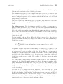
Figure 3 shows the path of a call into the call center. On this figure, rectangles represent
processing steps for the call while diamonds represent conditional branching. The rectangle
with thick lines represents the starting point of the calls in the system. An ellipse denotes
an outcome for a call (blocking, service, or abandonment). When a call arrives, a free agent
is selected among the I agent groups. The router (see section 2.4) uses the type of the call
to determine which agents are allowed to serve the call, and how agents are chosen if several
agents are free. If a free agent is found, the call is sent to that agent, and the agent is
allocated for a certain service time. Conditionnally on the call type, agent group and period
of arrival of the call, service times are i.i.d. and follow any parametric probability distribution
supported by SSJ. If no agent is available for a new call, the call is sent to a waiting queue if
that does not exceed the total queue capacity. With some probability depending on the call
type and the arrival period, independently of other events, the caller entering queue balks,
i.e., it abandons immediately. Other calls having to wait go into a queue where they remain
until agents are free to serve them. A queued caller can also become impatient, and abandon
without service. Patience times are i.i.d. conditionnal to call type, and arrival period. if the
queue is full at the time of a call’s arrival, the call is blocked instead of entering the queue,
i.e., the caller receives a busy signal.
6 2 SIMULATION MODEL
July 1, 2009
At least one free
agent?
Enter system
Yes
Blocking
Service
Abandonment
No
Yes
No
Yes
Queue full?
Yes
No
Balking?
No
Queue
Patience time
exceeded?
Figure 3: The path of a call in the call center
An agent finishing a service can disconnect for a random duration before it takes new
calls. The probability and duration of disconnecting may depend on the agent group, and
the time period. By default, the probability is 0, so no disconnecting occurs.
2.2.1
Inbound calls
Inbound calls are produced using some arrival processes. Such a process generates random inter-arrival times following some possibly non-stationary distributions, and generates
a single call upon each arrival. The most common distribution for inter-arrival times is exponential, which results in a Poisson arrival process. The simulator supports some variants
of the Poisson process with time-varying or stochastic arrival rates. Ssee section 8.3 for more
details.
2.2.2
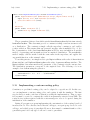
Outbound calls
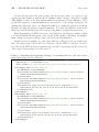
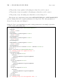
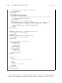
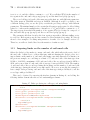
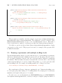
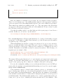
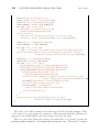
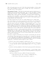
Outbound calls are produced using a predictive dialer which makes outbound calls when
certain conditions apply. There can be one dialer for each outbound call type as well as
dialers producing outbound calls of multiple, randomly-chosen, types.
When a dialer is started, it tries to perform outbound calls each time an agent capable
of serving calls produced by the dialer becomes free. Each time the dialer is triggered, it
decides on how many calls to try, and processes each of these calls independently, as shown
July 1, 2009
2.3 The agent groups 7
on figure 4. First, dialing succeeds with a reaching probability depending on the call type
and period. A delay depending on the success of the call, the call type, and the period
of dialing then occurs. The dialing delay can be used to model the party’s phone ringing
while a failed call may represent a busy signal, answering machine, etc. Successful calls are
processed in a similar way as inbound calls while failed calls simply leave the system after
they are counted. During the processing of a successful call, the period of arrival corresponds
to the period during which the dialer decided to make a call, not the period during which
the call entered the call center.
The only difference when processing inbound calls and successful outbound calls is the
service time which includes a preview time that can be used to model the work made by the
agent to determine if the right party is reached. The same way as service times, preview
times are i.i.d. but can depend on the call type, agent group, and period of arrival. After
this preview time, with some probability depending on the call type and period of arrival,
the call is a right party connect, and enters regular service. The preview and regular service
times are generated independently, and sum up in the case of right party connects. In other
words, the time the agent spends with an outbound call is the sum of the preview and service
times. On the other hand, if the call is a wrong party connect, it is counted separately and
excluded from reports concerning served calls. The service of a wrong party connect only
consists of a preview time.
No further special processing is applied to outbound calls in this model. However, some
parameters can be adapted to outbound calls. For example, a called customer often balks
(or abandons very quickly) if no agent is available to serve him. In fact, any outbound call
that needs to wait is called a mismatch, and is avoided in most call centers. Consequently,
the average patience time of any outbound call should be small.
The dialer uses a dialer’s policy to determine how many calls to dial each time it is
triggered. Let NFT (t) be the total number of free agents, or equivalently the number of free
D
(t) be the total number of free agents
agents in the test set, at simulation time t. Also let NF,k
capable of serving some calls produced by dialer k, or equivalently the number of free agents
in the target set for dialer k, at simulation time t.
D
A common dialing condition checks that NFT (t) ≥ st,k (t), and NF,k
(t) ≥ sd,k (t), where
st,k (t) and sd,k (t) are user-defined thresholds. Their values are constant during periods but
can change from periods to periods. The number of calls to dial at a time is computed
D
from NF,k
(t) in a way depending on the selected dialing policy. See section 8.4 for more
information.
2.3
The agent groups
Each agent group i has a fixed number Ni (t) of agents at any time during the simulated
horizon. In this model, the function Ni (t) is piecewise-constant. If Ni (t) increases at a given
time t, the additional agents are notified to the router which assigns them queued calls, if
possible. The type of the queued call assigned to a new agent in group i depends on the
routing policy being used.
8 2 SIMULATION MODEL
July 1, 2009
Fail delay
Failing
No
Dialing
Reached call?
Yes
Reach delay
Enter system
Figure 4: The path of an outbound call in the call center
Often, agents are added in several groups at a given time t, corresponding, e.g., to the
beginning of a main period. In such a case, the router notifies all new agents in group 0
to the router before notifying agents in groups 1, 2, etc. The order in which the agents are
notified to the router may have a small impact on which queued calls are assigned to which
agent groups, but this only affects a few calls.
If Ni (t) decreases at a given time t, no particular event happens, except if Ni (t) becomes
smaller than NB,i (t). The behavior of the system when that occurs depends on how the
agent group is modelled, but an agent always terminates its on-going service before it can
leave.
Only a fraction of the available agents is allowed to serve calls. If there is no busy agent,
the total number of agents free to serve calls is given by i Ni (t) rounded to the nearest
integer, where i ∈ [0, 1] is the efficiency of the agent group. If i = 1, all agents are allowed
to serve calls.
Agent groups can be modelled two ways by the simulator: with counters representing the
number of agents in each state, or with entities representing each individual agent. With
the first model, the agent group only retains the number of agents which are busy, free, and
idle but unavailable to serve calls. When Ni (t) < NB,i (t), on-going services are finished, and
the group does not accept any call until NB,i (t) < Ni (t). However, in the second model, the
so-called detailed group is composed of separate agents with their own states. In that case,
when Ni (t) < NB,i (t), some agents are marked to leave the system, but other busy agents
might finish their services before these marked agents leave. As a result, a detailed group
can accept new calls even when NB,i (t) > Ni (t). Which agents are marked is not relevant,
because all busy agents are identical in the model. Detailed agent groups are more realistic,
July 1, 2009
2.4 The router 9
and allow for computing the longest idle time of agents, which is needed by some routing
policies. However, using counter-based agent groups can increase performance compared to
detailed groups.
The Ni (t) functions can be specified three ways: with a staffing vector, with a schedule,
or with individual agents. In the first setting, Ni (t) remains constant during individual
periods. When specifying a schedule, one gives a set of shifts with arbitrary starting and
ending times, and assigns some agents to each shift. With the third mode, one assigns each
individual agent any user-defined properties in addition to a shift.
2.4
The router
A router assigns agents to inbound calls and successful outbound calls (agent selection or
push routing), and queued calls to free agents (call selection or pull routing), using a routing
policy to take its decisions. The model supports a set of predefined routing policies (see
section 8.5) that can be parameterized by the user.
The waiting queue represented on figure 1 is partitionned into several elementary waiting
queues implemented as lists. The number of waiting queues, and the way they are used
depend on the routing policy. Most routing policies assign a waiting queue to each contact
type, and all policies supported by the simulator use a First In First Out (FIFO) discipline
in individual queues.
Parameters for the routing policy are encoded in one of the three main data structures: a
set of ordered lists, incidence matrices, or matrices of ranks. When the first structure is used,
the type-to-group map defines an ordered list of agent groups ik,0 , ik,1 , . . . for each call type k.
These lists give the order in which agent groups are tested during agent selection. The
group-to-type map defines an ordered list of call types ki,0 , ki,1 , . . . for each agent group i.
These lists are used during call selection to determine the order in which call types are
tested. These routing tables are represented by non-rectangular 2D arrays of integers. In
the type-to-group map, there is one row for each call type whereas in the group-to-type map,
there is one row per agent group. Any negative integer in these 2D arrays being ignored,
they can be used for padding. For an example of a routing policy using this structure, see
QUEUEPRIORITY in section 8.5.
The second possible structure is a pair of incidence matrices. The type-to-group incidence
matrix defines a boolean function iTG (k, i) which determines if calls of type k can be routed
to agents in group i. The group-to-type incidence matrix defines a similar function iGT (i, k)
that determines if a call of type k can be selected by a free agent in group i. Often,
iTG (k, i) = iGT (i, k), i.e., a call of type k can be sent to an agent in group i if and only if a
free agent in group i can select a call of type k. These matrices are encoded into 2D arrays
of booleans. This structure is not used by any router at this moment.
When the third structure is used, the matrices of ranks, which can also be named the
priority matrices, define functions rTG (k, i) and rGT (i, k) giving the rank, i.e., priority, of
agents in group i for calls of type k. The lower is the rank, the higher is the preference of
the call type k for the agents in group i. When a rank is ∞, calls of type k cannot be served
10 2 SIMULATION MODEL
July 1, 2009
by agents in group i. The matrix defining the type-to-group ranks rTG (k, i), specifies how
contacts prefer agents, and is used for agent selection. On the other hand, the second matrix
defining the group-to-type ranks rGT (i, k) specifies how agents prefer contacts, and is used
for contact selection. In many cases, it is possible to have rGT (i, k) = rTG (k, i) and specify
a single matrix of ranks. These functions are encoded into rectangular 2D arrays of integers
containing, in the case of agent selection, one row for each contact type and one column for
each agent group. For contact selection matrices of ranks, the roles of rows and columns are
inverted. Although this structure is more flexible than ordered lists, it is often less intuitive
to figure out the implied routing. For an example of a routing policy using this structure,
see AGENTSPREF in section 8.5.
Routers using matrices of ranks often use complementary matrices of weights as well.
These are similar to matrices of ranks, except they define wTG (k, i) and wGT (i, k) functions
which are weights that can also be considered as penalties. These matrices default to matrices
of 1’s if they are not specified.
A last I × K matrix of delays can also be used to specify timers, i.e., d(i, k) gives the
minimal time a call of type k must wait before it can be served by an agent in group i.
2.5
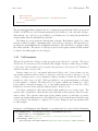
Call transfers
The model also supports transfers of calls from agents to agents, i.e., a primary agent serving
a call can transfer the call to a secondary agent. The agent transferring the call can either
hang up immediately after the transfer is initiated, or wait for the transfer to succeed or fail.
A transfer succeeds when a secondary agent can be assigned to the call, and fails if the call
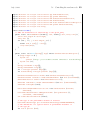
abandons before getting a secondary agent. The transfer process is summarized on figure 5.
More specifically, transfer works as follows. Let C be a call of type k arrived during
period p, and served by an agent A in group i. With probability rk,i,p , the call is transferred
to another agent after service. In that case, we suppose that the transfer decision is taken
before beginning of service, and multiply the service time of the call to be transferred by
mk,i,p , a constant depending on the call type, group of the serving agent, and main period
of arrival of the call. Let k 0 be the target random call type associated with call C for the
transfer. This new type index is generated randomly from a discrete distribution giving call
type k 0 a probability wk,p0 ,k0 depending on k and p0 .
A new call of type k 0 is created, and receives completely new attributes such as patience,
and service times. This new call C 0 is a virtual call corresponding to C.
A random delay depending on k, i, and p then occurs. This delay, which is 0 by default,
represents the time spent by the agent A to initiate the transfer, e.g., dialing a phone number.
After the delay, the new call C 0 is sent to the router the same way as an ordinary call. The
router’s policy can thus apply specific rules for type k 0 , which can differ from call type k.
Then, with probability 1 − qk,i,p , the agent A is freed although the transfer of the call is
not finished; this is sometimes called a cold transfer. On the other hand, with probability
qk,i,p , agent A waits for call C 0 to reach a free secondary agent B, or abandon; this is often
2.5 Call transfers 11
July 1, 2009
End of regular service
Transfer?
No
For primary call
Yes
New virtual call
Service
Transfer delay
Wait for secondary agent?
No
Free primary
agent if still
busy
No
Routing of virtual call
Secondary agent
found?
Yes
Conference with
primary agent (if
still busy)
No
Abandonment
Figure 5: The transfer of a call to a secondary agent
Service with
secondary agent
12 2 SIMULATION MODEL
July 1, 2009
denoted a warm transfer. In case of abandonment, calls C and C 0 end, and agent A is freed.
Note that call C is counted as a served call, even though C 0 abandons.
If service of call C 0 begins, and agent A is still waiting, a random conference time depending on type k 0 , period of transfer p0 , and secondary agent group i0 is generated. If this
conference time is greater than 0, it adds up to the regular service time of call C 0 (i.e., service
time is increased), and agent A waits for the conference time. Note that the conference time
is part of the service time both for call C, and call C 0 .
If service of call C 0 begins, but agent A is not waiting, another random pre-service time
occurs before the regular service time. This time can be used to model, e.g., a customer
identification process.
2.6
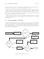
Virtual queueing or call backs
Some call centers make predictions of the waiting time of new customers, and offer them the
possibility to be called back at a later time if the predicted waiting time is too long. We
also say that customers to be called back join a virtual queue since the system must keep a
record of such customers in order to perform the callbacks. Virtual queueing is modelled as
shown on figure 6 in the simulator.
Call entering queue
Waiting time
prediction W
W smaller than
threshold?
Yes
Regular waiting
Second routing
of the call
No
No
Customer
call back?
Yes
Change of patience and service times
Waiting in
virtual queue
Yes
Call back
succeeds?
Figure 6: Virtual queueing of a call
Change of patience and service times
No
Blocking
July 1, 2009
2.7 Simulation experiments 13
More specifically, virtual queueing is allowed for a given call type k by setting a target
type index k 0 as well as a threshold for the expected waiting time. The index k 0 is used to
separate calls waiting in regular queue from calls sent to a virtual queue while the threshold
is used to test if the predicted queueing delay is sufficiently long for virtual queueing to
be worthwhile. When a call whose type allows virtual queueing arrives, an estimate of its
expected waiting time is obtained, using the last observed waiting time before a service as a
default heuristic. If this prediction W is smaller than a user-defined threshold Wk,p , where
p is the index of the main period of the call’s arrival, the call is processed normally.
Otherwise, with probability pk,p , the call exits the regular queue, and is sent to the
virtual queue. This models the fact that the center announces the predicted waiting time
to the caller, and the caller chooses to hang up and be called back at a later time. The
customer stays in the virtual queue for a fixed time given by W ∗ mk,p , where mk,p is a
user-defined multiplier defaulting to 1. With probability 1 − pk,p , the customer refuses to be
called back, and waits in the normal queue. However, the patience and service times of such
a customer is multiplied by user-defined factors fk,p and gk,i,p , respectively, which default
to 1. For example, a patience time multiplier greater than 1 can be used to model the fact
that customers knowing their expected waiting time could be more patient than customers
ignoring that information.
Before a call enters the virtual queue, its type identifier switches from k to k 0 . When the
customer leaves the virtual queue, call back occurs: with probability ck,p , call back succeeds,
and the call is sent back to the router to get a free agent, or to be queued again, hopefully
for a smaller time than if the customer had waited on the phone. Of course, the parameters
of the routing policy can be different for call types k and k 0 . For example, calls of type k 0
often have priority over calls of type k. With probability 1 − ck,p , call back fails, and the call
returning from the virtual queue is lost; it is counted as a blocked call in statistical reports.
Note that any random variable associated with the call having switched type for virtual
queueing is not generated a second time, from the distribution corresponding to type k 0 ; the
original values for call type k are kept. However, the patience and service times of a calls
returning from virtual queue are multiplied by factors hk,p , and ik,i,p , respectively. This can
be used, e.g., to model the fact that called back customers are not ready to wait as long as
regular customers.
2.7
Simulation experiments
Once the model parameters are set up, the simulator can perform experiments whose aim is to
estimate performance measures corresponding to expectations or functions of expectations.
Estimation is made using averages, or functions of averages, respectively.
Usually, one simulates the complete horizon of the model, and collects the resulting
estimates. The experiment is repeated several times with different random numbers in order
to i.i.d. observations for computing averages, functions of averages, confidence intervals, etc.,
for estimated performance measures. Without multiple replications, the estimators would
be too noisy to be useful.
14 2 SIMULATION MODEL
July 1, 2009
Alternatively, one can concentrate on a single period of the horizon, and simulate it as
if its duration was infinite in the model. The parameters of the model are then fixed for
the whole simulation, and the system is simulated for a certain time, usually larger than
the duration of the considered period. The simulator uses batch means [13, 5] to compute
confidence intervals on performance measures. See section 9 for more details about these
two types of experiments.
2.8
Simulation output
After any experiment, the simulator generates a report containing general information as well
as statistics for estimated performance measures. More specifically, the simulator computes
many (random) quantities on (constant) time intervals [t1 , t2 ] such as the number of calls
processed by the router (arrived calls), the number of served and blocked calls, calls which
have abandoned, etc. It also evaluates the integrals of the number of busy and working agents
over the interval [t1 , t2 ], for each agent group. The time interval can be the whole simulation,
a single period, etc., and statistics may be computed for several different intervals.
By default, a call arriving during period p is counted in statistics related to period p, even
if it exits the system during period p + 1. However, using the perPeriodCollectingMode
attribute in experiment parameters, one can make the simulator count the calls in the period
they leave the system.
Statistics are collected for main periods only. As a consequence, if the statistical period of
a call is the preliminary or wrap-up period, the call is not counted. Without this restriction,
the time interval of a statistic on the whole horizon would be random, and could change
from replications to replications.
Usually, a call is counted once. If a call switches from type k to k 0 due to virtual queueing,
it is counted as a type-k 0 call when call back fails, or at abandonment or end-service time.
However, when a call is transferred to another agent, the call served with the primary agent
is counted separately from the virtual call produced by the transfer.
A performance measure on a time interval [t1 , t2 ] can concern a segment of call types k,
a segment of agent groups i, or a pair (k, i). Here, a segment is simply a set regrouping call
types or agent groups. Let K 0 be the number of segments of call types. For more information
about segments, see sections 10.3 to 10.5.
Random variables concerning a fixed time interval can be regrouped into a random vector
X(t1 , t2 ) ∈ Rd . The expectation E[X(t1 , t2 )] is a vector of d possible performance measures
which can be estimated by a vector of averages X̄n (t1 , t2 ).
Other performance measures can be defined using functions g : Rd → R, and correspond to functions of expectations g(E[X(t1 , t2 )]) estimated using functions of averages
g(X̄n (t1 , t2 )). For example, by dividing the average sum of waiting times by the average
number of arrivals, we obtain the long term average waiting time over all calls which estimates the long term expected waiting time. Dividing the average number of busy agents by
the average number of agents gives the long term agents’ occupancy ratio.
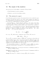
2.9 The simplified CTMC model 15
July 1, 2009
Another important performance measure is the service level defined as follows. Let
SG,k,p (sk,p ) be the number of contacts served after a waiting time less than or equal to sk,p ,
in inbound type segment k, and counted in period segment p. Let Sk,p be the total number
of served contacts in inbound type segment k counted in period segment p. The constant sk,p
is the acceptable waiting time, and can depend on k = 0, . . . , KI0 − 1 and p = 0, . . . , P 0 − 1.
Also let LG,k,p (sk,p ) be the number of contacts in inbound type segment k, counted in period
segment p, and having abandoned after a waiting time smaller than or equal to the acceptable
waiting time, and Ak,p be the total number of arrivals, for inbound type segment k, and period
segment p. The service level for inbound type segment k, and period segmen p is defined as
g1,k,p (sk,p ) =
E[SG,k,p (sk,p )]
.
E[Ak,p − LG,k,p (sk,p )]
Other definitions are possible for the service level, e.g.
g2,k,p (sk,p ) =
E[SG,k,p (sk,p ) + LG,k,p (sk,p )]
.
E[Ak,p ]
To make reporting easier, related performance measures are regrouped into matrices
whose rows represent segments of contact types or agent groups, and whose columns usually
represent time intervals. In some situations, there is a single period, which results in singlecolumn matrices. For example, the expected number of served calls of each type, and for
each period, estimated by averages, is such a group of performance measures.
Many other performance measures can be estimated by the simulator. See section 10.3 for
a complete list of supported performance measures. See also section 10 for more information
about how confidence intervals are computed, and the contents and possible formats of
statistical reports.
2.9
The simplified CTMC model
Simulation-based optimization requires many replications to evaluate the performance of a
call center for different configurations, e.g., with different staffing vectors. With the generic
multi-skill and blend simulator using the model described here, this is often too CPU intensive. The commonly used approximation formulas to work around this problem oversimplify
reality. An alternative simulator using a simplified continuous-time Markov chain (CTMC)
model is thus provided. This simulator generates transitions using the embedded discretetime Markov chain (DTMC), and computes expectations conditional to the sequence of
visited states.
The CTMC model used by this simulator is similar to the model described in this section,
with the following simplifications. First, arrivals always follow the Poisson process, patience
and times are exponential, there is no outbound call, no virtual queueing, no call transfer,
and agents cannot disconnect after service termination. Moreover, the queue capacity is
always finite.
16 2 SIMULATION MODEL
July 1, 2009
The following routing policy is used to select an agent for a new call. Each call type k
has a list Ik,0 , Ik,1 , . . ., where Ik,j is a set of agent groups, for j = 0, . . .. When a call of
type k arrives, if at least one free agent is available in one of the groups in Ik,0 , the call is
sent to a free agent in the group of Ik,0 containing the greatest number of free agents. If
several groups i ∈ Ik,0 contain the same maximal number of free agents, the group with the
maximal number of free agents, and the smallest index i is taken. On the other hand, if no
group in Ik,0 contains free agents, the sets Ik,1 , ik,2 , etc. are tested in a way similar to Ik,0 ,
in the order given by the list, to choose the first set with an agent group containing at least
one free agent. The sets Ik,j are constructed from the matrix of ranks given by the user. In
particular, the set Ik,0 is constructed by taking each agent group i with the minimal rank
rTG (k, i). The set Ik,1 is created by taking groups i with second smallest rank rTG (k, i).
For the selection of call at the end of service, each agent group has a list Ki,0 , Ki,1 , . . . of
sets of call types. First, if one waiting queue in Ki,0 contains at least one call, the service
starts for the call having spent the greatest number of DTMC transitions in queue, among
calls in queues of Ki,0 . If more than one call spent the greatest number of transitions in
queue, the call with the greatest number of transitions in queue and the smallest index k
is taken. On the other hand, if no queue in Ki,0 contains calls, the sets Ki,1 , Ki,2 , etc. are
checked in a way similar to Ki,0 , in the order given by the list, to find the first set with
a queued call. In a way similar to Ik,j , the sets Ki,j are constructed by using the values
rGT (i, k) taken from the matrix of ranks given by the user.
July 1, 2009
3
17
Examples of data files
The configuration of the simulator is specified by at least two XML files. A XML [21] file
contains a hierarchical structure of elements with possible attributes and nested contents. An
overview of XML and data structures supported by the simulator is provided in section 8.1.
The first file specifies the parameters for the call center itself. These parameters are
usually determined by a manager based on a real system. The second file specifies parameters
for the simulation experiment, such as the simulation length, the required target relative
error, etc. These parameters are determined by the simulation expert at the time experiments
are performed. Two formats are available for encoding parameters describing experiments:
a first one for the batch means method and a second one for simulation using independent
replications.
In this section, we present examples of parameter files for different models of call centers.
We start with a single queue, and extend it by adding a new call type, a new agent group,
etc. The last examples are blend call centers with one inbound call type and one outbound
call type. The last example is a blend and multi-skill call center demonstrating most of the
possibilities of the simulator.
3.1
Single queue
This example models a call center with a single call type, a single agent group, but multiple
time periods. Each day, the center operates for P hours. The parameters can change during
the day, but they are constant within each hour.
Calls arrive following a Poisson process with piecewise-constant arrival rate λp during
period p, where λp is constant. Calls that cannot be served immediately are put in a FIFO
queue, and abandon if they wait more than their patience time. The i.i.d. patience times
are generated as follows: with probability ρ, the patience time is 0, i.e., the caller abandons
if he cannot be served immediately. With probability 1 − ρ, the patience time is exponential
with mean 1/ν. Service times are i.i.d. exponential random variables with mean 1/µ.
During main period p, Np agents are available to serve calls. If, at the end of period p,
the number of busy agents is larger than Np+1 , ongoing calls are completed, but new calls are
not accepted until the number of busy agents is smaller than Np+1 . During the preliminary
period, there is no agent whereas for the wrap-up period, NP +1 = NP . Listing 1 presents
the XML file for this example.
Listing 1: singleQueue.xml: Example of a parameter file for a call center with a single
queue
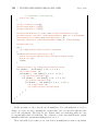
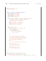
<ccmsk:MSKCCParams
defaultUnit="SECOND" periodDuration="PT1H"
numPeriods="13" startingTime="PT8H"
xmlns:ccmsk="http://www.iro.umontreal.ca/lecuyer/contactcenters/msk">
<inboundType name="Inbound Type">
<probAbandon>0.1</probAbandon>
18 3 EXAMPLES OF DATA FILES
July 1, 2009
<patienceTime distributionClass="ExponentialDistFromMean" unit="SECOND">
<defaultGen>1000</defaultGen>
</patienceTime>
<serviceTime distributionClass="ExponentialDistFromMean" unit="SECOND">
<defaultGen>100</defaultGen>
</serviceTime>
<arrivalProcess type="PIECEWISECONSTANTPOISSON" normalize="true">
<arrivals>100 150 150 180 200 150 150 150 120 100 80 70 60</arrivals>
</arrivalProcess>
</inboundType>
<agentGroup name="Agents">
<staffing>4 6 8 8 8 7 8 8 6 6 4 4 4</staffing>
</agentGroup>
<router routerPolicy="AGENTSPREF">
<ranksTG>
<row>1</row>
</ranksTG>
<routingTableSources ranksGT="ranksTG"/>
</router>
<serviceLevel name="20s">
<awt>
<row>PT20S</row>
</awt>
<target>
<row>0.8</row>
</target>
</serviceLevel>
<serviceLevel name="30s">
<awt>
<row>PT30S</row>
</awt>
<target>
<row>0.8</row>
</target>
</serviceLevel>
</ccmsk:MSKCCParams>
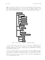
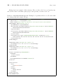
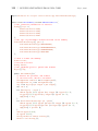
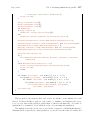
The XML file presented here is composed of elements and attributes describing the hierarchical data. In a XML document, elements are used to represent complex data. Each element
has a tag name, e.g., serviceTime, opening and closing markers (e.g., <serviceTime>, and
</serviceTime>), a set of attributes, and nested contents. An attribute is a key-value pair
representing simple data associated to an element while nested contents can be simple text
or children elements. Each document has a single root element which can have an arbitrary
3.1 Single queue 19
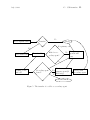
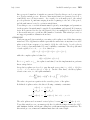
July 1, 2009
number of attributes and children. See section 8 for more information. The elements of any
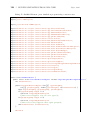
XML document can be represented as a tree such as the one displayed on figure 7. The
figure shows that MSKCCParams is the root of the tree, and has one child for the inbound call
type, one child for the agent group, etc. We now describe the XML file in more details.
MSKCCParams
inboundType
probAbandon
patienceTime
serviceTime
arrivalProcess
agentGroup
staffing
router
ranksTG
routingTableSources
serviceLevel
awt
target
Figure 7: The hierarchical structure of example in Listing 1
For call center parameters, the name of the root element must be MSKCCParams with
a namespace URI set to http://www.iro.umontreal.ca/lecuyer/contactcenters/msk.
The xmlns:ccmsk attribute of this root element is used to bind this URI to the shorter
prefix ccmsk in the parameter file.
The root element is allowed to have some attributes such as periodDuration (main
period duration d), defaultUnit (default time unit), etc., as well as children elements.
The attributes of an element are given after the name of the element, and before the >
marker. Nested contents of the root element is located between the <ccmsk:MSKCCParams>
and </ccmsk:MSKCCParams> markers.
20 3 EXAMPLES OF DATA FILES
July 1, 2009
In this model, 13 periods of one hour are set up by setting numPeriods to 13 and periodDuration to PT1H. The notation for time durations, which seems confusing at first sight, is
imposed by the XML Schema Specification (see section 8.2.1, and [19, part 2, section 3.2.6]).
The attribute defaultUnit, set to SECOND in this example, sets the implicit unit for time
durations. This is the time unit used during simulation as well as the unit of any time-related
output, e.g., waiting time.
Nested elements are used to describe more complex information such as call types, agent
groups, the router, and the parameters for estimating the service level. The order of these
elements must not be changed for the parameter file to remain valid. It is also important to
keep the hierarchy of the document, e.g., the router element should not be moved inside an
inboundType element.
We now describe the contents of the inboundType element, which represents the call type
in this example, in more details. First, the name attribute is used to bind a name to the
inbound call type. A name can also be associated with an agent group.
The probAbandon element is used to set the probability of balking, for each main period.
This element accepts an array of values on the [0, 1] interval. If the array contains a single
value such as in this example, the value is automatically reused for all periods. Therefore,
the user does not need to repeat 0.1 13 times to have ρ = 0.1 for all periods in this example.
The way patience and service times are specified differ from the way the period duration is given, because these aspects of the model require probability distributions, not only
mean time durations. The distribution for patience time is given using the patienceTime
element whose type corresponds to a probability distribution. Such an element accepts a
distributionClass attribute giving the SSJ class of the probability distribution while the
defaultGen child element sets the distribution parameters. The latter element accepts an array giving the arguments passed to the constructor of the chosen distribution class. The role
of these arguments depends on the chosen distribution class, and do not always correspond
to means and variances.
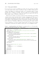
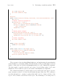
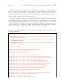
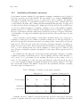
Table 1 gives the parameters for the most commonly used distributions. The first column
gives the name of the class, i.e., the value of the distributionClass attribute, corresponding to the distribution. The other columns give the density of the distribution, its mean,
its variance, and the order of parameters required for the distribution. See the package
umontreal.iro.lecuyer.probdist in the user’s manual of SSJ [14] for additional distributions.
According to table 1 or the SSJ documentation from [14], the exponential distribution is
represented by the ExponentialDistFromMean class, and has a scale parameter µ representing the mean which needs to be specified as an argument for calling the constructor. Here,
µ = 1000. The unit attribute of patienceTime specifies that the generated patience times
must be considered in seconds, so the mean patience time is 1000s for this example. The
serviceTime element has the same structure as patienceTime, but it gives the service time
distribution for calls, served by any agent.
The arrivalProcess element specifies the arrival process to be used for this inbound call
type, along with its parameters. The type attribute is used to indicate the type of arrival
3.1 Single queue 21
July 1, 2009
Table 1: Parameters for the most commonly used probability distributions
distributionClass
ExponentialDist
ExponentialDistFromMean
GammaDist
GammaDistFromMoments
NormalDist
LognormalDist
Density f (x)
λe−λx for x ≥ 0
e−x/µ /µ for x ≥ 0
−λx
λα xα−1 eΓ(α) , for x > 0
exp(−(x−µ)2 /(2σ 2 ))
√
2πσ
exp(−(ln(x)−µ)2 /(2σ 2 ))
√
,
2πσx
Mean
1/λ
µ
α/λ
m
µ
eµ+σ
2 /2
Variance
1/λ2
µ2
α/λ2
v
σ2
2
Parameters
λ>0
µ>0
α > 0, λ > 0
m, m > 0
µ, σ > 0
2
e2µ+σ (eσ − 1) µ, σ > 0
for x > 0
LognormalDistFromMoments
m
v
m > 0, v > 0
R∞
Here, Γ(α) = 0 xα−1 e−x dx. In particular, Γ(n) = (n − 1)! when n is a positive integer.
The gamma and lognormal distributions with moments have the same density as ordinary
the gamma and lognormal distributions, but a mean and a variance are entered rather than
shape and scale parameters.
process, which can be any string specified in section 8.3. The arrivals vector element gives
the parameters for the arrival process, in this case the Poisson arrival rate. By default,
this arrival rate corresponds to the expected number of calls during a simulation time unit,
i.e., one second in our setting. By setting the normalize attribute to true, we instruct the
simulator to interpret the arrival rates as relative to one period. Consequently, the given
arrival rates set the expected number of arrivals during each hour for this example.
The agentGroup element describes the agent group in the call center. The staffing
child element is used to associate a staffing with the agent group. It contains an array
giving the number of agents during each main period of the day. Alternatively, the array
can contain a single element; the staffing will then be fixed for the whole day.
Then, the agentGroup element is used to describe the agent group of the example. We
give a name to the agent group using the name attribute and configure its staffing using the
staffing element. This gives a number of agents for each main period of the model.
The router element is then used to describe how routing is done in the model. Here, we
have a very basic routing sending any incoming call to a free agent. For this, the routerPolicy attribute is used to configure the router’s policy. Here, we use the AGENTSPREF
policy which is very general. But we could use other more efficient policies for this example.
Section 8.5 describes in details the available router’s policies.
The selected router’s policy minimally requires a K × I matrix associating a priority to
each (call type, agent group) pair during agent selection, and a second I × K matrix setting
the priorities similarly during call selection. The first matrix is set using ranksTG (ranks for
type-to-group assignments) while the second matrix is given using ranksGT (ranks for groupto-type assignments). A matrix can be represented by a sequence of arrays in the parameter
file, each array being represented by a row child element. Here, we use the 1 × 1 identity
22 3 EXAMPLES OF DATA FILES
July 1, 2009
matrix for both parameters. The second matrix can be given explicitly using the ranksGT.
However, instead of transposing the contents of ranksTG manually to obtain ranksGT when
rTG (k, i) = rGT (i, k) for all k and i, we can instruct the router to generate ranksGT by
transposing ranksTG, by using the routingTableSources element. This will become useful
when we increase the number of call types and agent groups.
The serviceLevel element gives thresholds for the service level using two KI0 × P 0 matrices: one for the acceptable waiting times, and a second one for the service level targets.
Often, KI0 = KI + 1 if KI > 1, and KI otherwise, and P 0 is defined similarly using P . Several
serviceLevel elements, with different awt and target matrices, can be specified to set
the values for different contact types and periods. The targets are not considered during
simulation, but they can be used by optimization programs.
However, these matrices are sometimes sparse, i.e., the user only specifies some values.
Consequently, if a matrix of thresholds (or targets) contains a single element, its single value
is used for all call types and periods. If it contains a single row or column, the row or column
is duplicated as required.
Here, we set the acceptable waiting time to 20s, and the service level target to 80%.
We need 1 × 1 matrix containing PT20S, and 0.8, respectively. We also specify a second
threshold of 30s with target 80% by using a second serviceLevel element.
After the model parameters are configured, simulation parameters are needed in order
to perform experiments. The simplest method of experiment consists of simulating a fixed
number of independent replications. This can be described by a file similar to Listing 2.
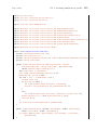
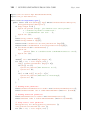
Listing 2: repSimParams.xml: Example of a parameter file for an experiment using independent replications
<ccapp:repSimParams minReplications="300"
xmlns:ccapp="http://www.iro.umontreal.ca/lecuyer/contactcenters/app">
<report confidenceLevel="0.95"/>
</ccapp:repSimParams>
The root element for the parameter file is repSimParams with namespace URI http://
www.iro.umontreal.ca/lecuyer/contactcenters/app, which differs from the namespace
URI of MSKCCParams. The number of performed runs is fixed to 300 by the minReplications
attribute.
The report element contains the parameters of the statistical report produced by the
simulator. In particular, the confidenceLevel attribute sets the confidence level of intervals
to 95%. These confidence intervals are computed using the normal assumption (see section 10
for more details). The report is printed when the simulator is invoked from the commandline or when the formatStatistics method is called from a Java program. This includes
the confidence level of the printed intervals as well as the statistics to include in the report.
Here, no information is provided about printed statistics so the report includes information
about all supported performance measures.
July 1, 2009
3.2
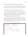
3.2.1
3.2 Variants of the single-queue model 23
Variants of the single-queue model
Disabling abandonment
In some situations, it can be necessary to disable abandonment, e.g., if no information about
patience is available, or if simulation needs to be compared with approximation formulas.
Doing this increases the workload of the simulated agents, because customers abandoning
must now all be served. This increases the waiting time, and decreases the service level
if the number of agents is not increased to compensate this. Of course, a model without
abandonment is less realistic than an equivalent model with abandonment.
Abandonment can be disabled by removing probAbandon and patienceTime from the
XML file. Removing probAbandon disables balking by setting the probability of immediate
abandonment to 0 while removing patienceTime sets all patience times to infinity.
Removing an element from a XML file can be performed by destructively deleting all the
text representing the element, and its children, or by commenting it out. For example, the
following code represents a patience time which was commented out:
<!-<patienceTime distributionClass="ExponentialDistFromMean" unit="SECOND">
<defaultGen>1000</defaultGen>
</patienceTime>
-->
The sequences <!-- and --> serve as comment delimiters in the XML language. Since comments are ignored by the parameter reader, they can be used to store additional information
about the parameter file. This information is intended to be used by human beings only. Any
information used by a computer program should be encoded in XML elements, attributes,
or nested text.
3.2.2
Setting period-specific parameters
The example on Listing 1 sets a stationary distribution for the patience and service times.
If the distribution of the service times can change from periods to periods, one can replace
the defaultGen element of serviceTime with a sequence of periodGen elements, as shown
on the next listing.
<serviceTime distributionClass="ExponentialDistFromMean"
<periodGen>100</periodGen>
<periodGen>150</periodGen>
<periodGen>180</periodGen>
<periodGen>90</periodGen>
<periodGen>110</periodGen>
</serviceTime>
unit="SECOND">
24 3 EXAMPLES OF DATA FILES
July 1, 2009
This sets the per-period mean service time, for a model defining five main periods. The
pth periodGen element gives the parameters of the service time for main period p, with
p = 1, . . . , P . Of course, the number of periodGen elements must correspond to the number
of main periods in the model.
3.2.3
Increasing the variability of arrivals
With the arrival process of the original model, the number of arrivals during period p follows
the Poisson distribution with mean λp , and variance λp . This variance can be increased
randomizing the arrival rate in each period. The arrival process is then doubly stochastic.
For example, this can be done by setting the arrival rates to Bλp , where B is a random
variable with mean 1. The random variable B, generated each day, represents the busyness
factor of the day. The day is more busy than usual when B > 1 and less busy than usual
when B < 1. A well-studied distribution for B is gamma with equal parameters α0 [3]. Such
a busyness factor can be used by adding the busynessGen element before any inboundType
element, e.g.,
<busynessGen distributionClass="GammaDist">10 10</busynessGen>
This sets the distribution of the busyness factor to gamma(10,10). This element does not
accept defaultGen or periodGen children, because the busyness factor is generated once at
the beginning of the day, and thus does not change from periods to periods.
Another way of increasing the variance of the number of arrivals is to use a Poisson-gamma
arrival process where the arrival rate for each period is gamma-distributed, independently
of other periods. This can be specified as follows:
<arrivalProcess type="POISSONGAMMA" normalize="true">
<poissonGammaShape>100 150 150 180 200 150 150 150
120 100 80 70 60</poissonGammaShape>
<poissonGammaScale>1 1 1 1 1 1 1 1
1 1 1 1 1</poissonGammaScale>
</arrivalProcess>
Here, we have changed the value of the type attribute to POISSONGAMMA, and replaced the
arrivals element with poissonGammaShape, and poissonGammaScale. These new elements
give the gamma shape and scale parameters for each main period. Section 8.3 gives the list
of all available arrival processes, with a detailed description for each one.
3.2.4
Changing the number of periods
Increasing the number of periods often requires several updates in the parameter file. First,
the numPeriods attribute in MSKCCParams must be modified. Then, each element defining
July 1, 2009
3.2 Variants of the single-queue model 25
period-specific parameters must be updated with the new periods. This includes balking
probabilities stored in probAbandon elements, patience and service times stored in patienceTime and serviceTime elements, arrival process (arrivals elements for Poisson processes
with piecewise-constant rates), staffing in staffing elements, and service level information
in serviceLevel elements. Missing per-period parameters will result in error messages when
running the simulator. If an element sets parameters for more periods than the value given
by numPeriods, the last extra periods are ignored.
3.2.5
Adding a new call type
Adding a new call type is a three-steps process:
1. Adding a new inboundType element;
2. Adapting the routing policy for a new call type;
3. Extending the matrices of AWTs and targets for the service level.
We now describe these steps in more details.
Adding a new inboundType element can be done by copying the contents of an existing
inboundType element, and altering its contents. The main issue to consider is the indexing
of call types: adding new call types can shift indices, and require adjustments in other parts
of the XML file. More specifically, each call type receives an index based on its order of
occurrence in the XML file. This index is used for specifying type-to-group and group-totype maps for some routing policies as well as target call types for call transfers and virtual
queueing. See section 3.4 for an example with a type-to-group map.
In our original setting, the only call type has index 0. Adding a new inboundType
element just below the original one creates a new call type with index 1. However, adding
the element before the original inboundType element assigns index 0 to the new call type,
and shifts the index of the old call type to 1. This can cause problems especially if the model
already contains several call types.
The second step in adding the call type is to update the parameters of the routing policy.
In our example, we need to change the ranksTG child element of router in order to extend
the matrix of ranks with a new row. This new row sets the priorities for the new type.
Failing to do that will result in errors preventing the simulator to run.
With a single agent group and the agents’ preference-based routing policy, if both call
types have the same priority, agents becoming free select the call with the longest waiting
time. Otherwise, free agents first look for calls with the lowest rank (i.e., highest priority)
before calls with the highest rank.
If call type 1 has priority over call type 2, or even if its mean service time is shorter than
the mean service time of call type 2, calls of type 1 will wait less before they get service, and
therefore will have higher service level than calls of type 2.
26 3 EXAMPLES OF DATA FILES
July 1, 2009
If both call types have the same priority, and mean service time, one expects to get
exactly the same results as with the model defining a single call type. In practice, results
differ slightly because of the way random numbers are generated by the simulator. More
specifically, sequences of random numbers are associated to each call type separately. By
splitting the calls in two types, one changes the number of constructed sequences of random
streams, and thus the generated random numbers. Note that the difference between the
single-type and the two-types model decreases as the number of replications increases.
Extending matrices of AWTs and service level targets is optional if it contains a single
row, and the thresholds and targets do not depend on the call type. Otherwise, the matrices
must contain one row per call type, plus a row for the global parameters.
Listing 3 gives an example of a call center with two call types, and one agent group.
Here, the target service level is 80% for both types, but the AWT for call type 2 is set to
60s. The global AWT and target remain at 20s, and 80%, respectively. In the new model,
calls of type 1 have priority over calls of type 2.
Listing 3: singleQueueTwoTypes.xml: Example of a parameter file for a call center with a
single agent group and two call types
<ccmsk:MSKCCParams
defaultUnit="SECOND" periodDuration="PT1H"
numPeriods="13" startingTime="PT8H"
xmlns:ccmsk="http://www.iro.umontreal.ca/lecuyer/contactcenters/msk">
<inboundType name="Inbound Type 1">
<probAbandon>0.1</probAbandon>
<patienceTime distributionClass="ExponentialDistFromMean" unit="SECOND">
<defaultGen>1000</defaultGen>
</patienceTime>
<serviceTime distributionClass="ExponentialDistFromMean" unit="SECOND">
<defaultGen>100</defaultGen>
</serviceTime>
<arrivalProcess type="PIECEWISECONSTANTPOISSON" normalize="true">
<arrivals>75 100 100 100 100 30 50 80 90 70 40 40 10</arrivals>
</arrivalProcess>
</inboundType>
<inboundType name="Inbound Type 2">
<probAbandon>0.1</probAbandon>
<patienceTime distributionClass="ExponentialDistFromMean" unit="SECOND">
<defaultGen>1000</defaultGen>
</patienceTime>
<serviceTime distributionClass="ExponentialDistFromMean" unit="SECOND">
<defaultGen>150</defaultGen>
</serviceTime>
<arrivalProcess type="PIECEWISECONSTANTPOISSON" normalize="true">
<arrivals>25 50 50 80 100 120 100 70 30 30 40 30 50</arrivals>
</arrivalProcess>
</inboundType>
July 1, 2009
3.2 Variants of the single-queue model 27
<agentGroup name="Agents">
<staffing>4 6 8 8 8 7 8 8 6 6 4 4 4</staffing>
</agentGroup>
<router routerPolicy="AGENTSPREF">
<ranksTG>
<row>1</row>
<row>2</row>
</ranksTG>
<routingTableSources ranksGT="ranksTG"/>
</router>
<serviceLevel>
<awt>
<row>PT20S</row>
<row>PT60S</row>
<row>PT20S</row>
</awt>
<target>
<row>0.8</row>
<row>0.8</row>
<row>0.8</row>
</target>
</serviceLevel>
</ccmsk:MSKCCParams>
3.2.6
Adding a new agent group
Adding a new agent group involves two steps similar to adding a call type:
1. Adding a new agentGroup element;
2. Adapting the routing policy;
We will now describe these steps in more details.
A new agentGroup element can be added by copying an existing element, and altering
parameters. Usually, the name and staffing of the agent group are adapted. As with call
types, adding agent groups can shift indices as we discussed in the previous subsection.
The routing policy is adapted by adding a new column to the matrix of ranks of the
model. This is done by updating the ranksTG element in the parameter file. This new
column sets priorities concerning the new agent group. With a single call type, if two agent
groups have the same priority, a newly-arrived call is assigned to the agent with the longest
idle time among the two groups. If ranks are different, the agent group with the lowest rank
(i.e., highest priority) is checked for agents before the group with higher rank.
28 3 EXAMPLES OF DATA FILES
July 1, 2009
Listing 4 gives an example of this extension. Here, we have added a second agent group,
and set the router for the first agent group to have priority over the second one.
Listing 4: singleQueueTwoGroups.xml: Example of a parameter file for a call center with
two agent groups and a single call type
<ccmsk:MSKCCParams
defaultUnit="SECOND" periodDuration="PT1H"
numPeriods="13" startingTime="PT8H"
xmlns:ccmsk="http://www.iro.umontreal.ca/lecuyer/contactcenters/msk">
<inboundType name="Inbound Type">
<probAbandon>0.1</probAbandon>
<patienceTime distributionClass="ExponentialDistFromMean" unit="SECOND">
<defaultGen>1000</defaultGen>
</patienceTime>
<serviceTime distributionClass="ExponentialDistFromMean" unit="SECOND">
<defaultGen>100</defaultGen>
</serviceTime>
<arrivalProcess type="PIECEWISECONSTANTPOISSON" normalize="true">
<arrivals>100 150 150 180 200 150 150 150 120 100 80 70 60</arrivals>
</arrivalProcess>
</inboundType>
<agentGroup name="Inbound-only
<staffing>1 4 4 3 2 4 5 6 5
</agentGroup>
<agentGroup name="Inbound-only
<staffing>3 2 4 5 6 3 3 2 1
</agentGroup>
agents 1">
5 2 3 3</staffing>
agents 2">
1 2 1 1</staffing>
<router routerPolicy="AGENTSPREF">
<ranksTG>
<row>1 2</row>
</ranksTG>
<routingTableSources ranksGT="ranksTG"/>
</router>
<serviceLevel>
<awt>
<row>PT20S</row>
</awt>
<target>
<row>0.8</row>
</target>
</serviceLevel>
</ccmsk:MSKCCParams>
July 1, 2009
3.2 Variants of the single-queue model 29
If we simulate with this parameter file, we obtain a warning about agent groups not
in detailed mode. This is caused by the fact that in general, the routing policy we have
chosen requires the longest idle times of agents to break tie for agent groups sharing the
same minimal rank. This idle time can be obtained only when agent groups are in detailed
mode, i.e., if they model each agent as separate objects. However, for this example, idle
times are not needed, because all ranks are different.
The warning can be removed two ways: by setting the detailed attribute to true for
each agentGroup element, or by setting the agentSelectionScore attribute of the router
element to something other than LONGESTIDLETIME, e.g., NUMFREEAGENTS. The first solution
switches the agent groups to detailed mode, which allows the idle times to be retrieved, while
the second alternative changes how tie is broken for agent groups sharing the same minimal
rank.
3.2.7
Adding routing delays
With the routing policy used in this model, agent groups are queried sequentially in order
to find a free agent to serve a newly-arrived call; this is call overflow routing. Similarly,
call types are looked up sequentially in order to find a call for a free agent; this is denoted
priority queueing. Sometimes, we need the router to wait for some time between each agent
group, and call type. This can be done by setting delays in the router’s parameters.
First, the routing policy has to be switched from AGENTSPREF to AGENTSPREFWITHDELAYS.
Then, a I × K matrix of time durations is specified using delaysGT element Each element
(i, k) of the matrix gives the minimal time a call of type k has to wait in queue before it can
be served by any agent in group i.
As an example, suppose we combine the two extensions proposed in the preceding subsections. We therefore have two call types, and two agent groups. We then assign each call
type k = 0, 1 a primary agent group i, but we allow the other agent group to serve the
call, with lower priority, and a minimal delay of 30s. The resulting router element looks as
follows:
<router routerPolicy="AGENTSPREFWITHDELAYS">
<ranksTG>
<row>1
2</row>
<row>2
1</row>
</ranksTG>
<delaysGT>
<row> PT0S
PT30S</row>
<row>PT30S
PT0S</row>
</delaysGT>
<routingTableSources ranksGT="ranksTG"/>
</router>
Note that setting any rank for a (k, i) pair to ∞, by replacing the numerical value with INF,
prevents the router from assigning calls of type k to agents in group i.
30 3 EXAMPLES OF DATA FILES
3.2.8
July 1, 2009
Using agent schedules
For any agent group described in a XML file representing call center parameters, the staffing
vector can be replaced with a schedule. Schedules are composed of shifts to which agents are
assigned. The staffing vector is thus replaced with a vector containing the number of agents
per shift, with a description of the shifts. The most common way of specifying schedule
shifts is to give a J × P matrix of booleans whose element (j, p) is true if and only if an
agent working on shift j is scheduled for main period p.
Listing 5 gives an example of an agent group with a schedule. In this listing, the staffing
element is replaced with a schedule element containing a numAgents child. This vector of
agents instructs the simulator to schedule one agent for each shift. The matrix of shifts is
set up using the element shiftMatrix which is placed after the element describing the agent
group. Each row of the matrix corresponds to a shift while each column concerns a main
period of the model. The matrix of shifts is used for every agent group for which a schedule
is given. Alternatively, one can give a matrix of shits specific to an agent group by putting
a shiftMatrix element inside the schedule element, just before the numAgents element.
Listing 5: singleQueueShifts.xml: Example of a parameter file for a call center with a
single agent group with a schedule, and a single call type
<ccmsk:MSKCCParams
defaultUnit="SECOND" periodDuration="PT1H"
numPeriods="13" startingTime="PT8H"
xmlns:ccmsk="http://www.iro.umontreal.ca/lecuyer/contactcenters/msk">
<inboundType name="Inbound Type">
<probAbandon>0.1</probAbandon>
<patienceTime distributionClass="ExponentialDistFromMean" unit="SECOND">
<defaultGen>1000</defaultGen>
</patienceTime>
<serviceTime distributionClass="ExponentialDistFromMean" unit="SECOND">
<defaultGen>100</defaultGen>
</serviceTime>
<arrivalProcess type="PIECEWISECONSTANTPOISSON" normalize="true">
<arrivals>100 150 150 180 200 150 150 150 120 100 80 70 60</arrivals>
</arrivalProcess>
</inboundType>
<agentGroup name="Inbound-only agents">
<schedule>
<numAgents>1 1 1 1 1 1 1</numAgents>
</schedule>
</agentGroup>
<shiftMatrix>
<row>1 1 1 1 0 1 1 0 0 0 0 0 0</row>
<row>0 1 1 1 1 0 1 1 0 0 0 0 0</row>
<row>0 0 1 1 1 1 0 1 1 0 0 0 0</row>
<row>0 0 0 1 1 0 1 1 1 1 0 0 0</row>
3.2 Variants of the single-queue model 31
July 1, 2009
<row>0 0 0 0 1
<row>0 0 0 0 0
<row>0 0 0 0 0
</shiftMatrix>
1
1
0
1
1
1
0
1
1
1
1
1
1
0
1
1
1
0
0
1
1
0</row>
0</row>
1</row>
<router routerPolicy="AGENTSPREF">
<ranksTG>
<row>1</row>
</ranksTG>
<routingTableSources ranksGT="ranksTG"/>
</router>
<serviceLevel>
<awt>
<row>PT20S</row>
</awt>
<target>
<row>0.8</row>
</target>
</serviceLevel>
</ccmsk:MSKCCParams>
The simulator also accepts shifts represented as time intervals. These are specified in the
XML parameter file using shift elements. For example, the first row of the matrix of shifts
in the above example may be written as follows.
<schedule>
<shift numAgents="1">
<shiftPart startingTime="PT8H" endingTime="PT12H" type="Working"/>
<shiftPart startingTime="PT13H" endingTime="PT15H" type="Working"/>
</shift>
</schedule>
With this input method, the starting and ending times of shifts do not need to match with
a change of main period.
3.2.9
Estimating parameters
When modeling a call center, the probability distributions of the random variables is unknown. A common solution to this problem is to guess a parametric probability distribution
and fit real data to this distribution. The generic simulator can estimate parameters from
data for probability distributions and some arrival processes by using the maximum likelihood method. For this, data can be specified directly in parameter files. Listing 6 presents
the parameter file of the example in Listing 1, with some parameters replaced with artificial
data.
32 3 EXAMPLES OF DATA FILES
July 1, 2009
Listing 6: singleQueueMLE.xml: Example of a parameter file with data for parameter estimation
<ccmsk:MSKCCParams defaultUnit="SECOND" periodDuration="PT1H"
numPeriods="13"
startingTime="PT8H"
xmlns:ccmsk="http://www.iro.umontreal.ca/lecuyer/contactcenters/msk">
<inboundType name="Inbound Type">
<probAbandon>0.1</probAbandon>
<patienceTime distributionClass="ExponentialDist" unit="SECOND">
<defaultGen>0.001</defaultGen>
</patienceTime>
<serviceTime distributionClass="ExponentialDist" unit="SECOND">
<!-- i.i.d. exponentials with lambda=0.01 -->
<defaultGen estimateParameters="true">
13.583 38.350 36.988 174.782 25.055 76.227 65.542 43.937
<!-- more observations here -->
</defaultGen>
</serviceTime>
<arrivalProcess type="PIECEWISECONSTANTPOISSON" normalize="true"
estimateBusyness="true">
<!-- Observations generated from the Poisson distribution -->
<data>
<row>89 144 144 193 189 151 149 145 108 107 82 68 56</row>
<row>93 153 166 173 175 173 137 158 110 86 73 74 53</row>
<row>100 140 154 190 217 164 162 157 120 86 65 83 76</row>
<row>99 153 155 143 222 146 151 157 125 89 81 58 66</row>
<!-- More observations -->
</data>
</arrivalProcess>
</inboundType>
<agentGroup name="Inbound-only agents">
<staffing>4 6 8 8 8 7 8 8 6 6 4 4 4</staffing>
</agentGroup>
<router routerPolicy="AGENTSPREF">
<ranksTG>
<row>1</row>
</ranksTG>
<routingTableSources ranksGT="ranksTG"/>
</router>
<serviceLevel>
<awt>
<row>PT20S</row>
</awt>
<target>
<row>0.8</row>
July 1, 2009
3.3 Additional experiment parameters 33
</target>
</serviceLevel>
</ccmsk:MSKCCParams>
Data is specified at the same place as regular parameters, except that the estimateParameters attribute is set to true. For probability distributions over the real numbers
(continuous or discrete), this element is an array of double-precision values. For discrete
distributions over the integers, the double-precision values of the data are rounded to the
nearest integers.
For an arrival process, one must use the data element which accepts a matrix of integers
giving the observed number of arrivals during each main period for observed days. The
parameters of arrival processes are estimated by considering each given P -dimensional vector
representing a day as independent and identically distributed.
For arrival processes, parameter estimation is more complex, because the number of
arrivals in all periods comes from a multivariate distribution, and some methods estimate
the parameters of the busyness factor and the arrival rates simultaneously. For these reasons,
the way parameters are estimated for arrival processes depends on the specific type of process,
and the value of the estimateBusyness attribute. For example, with the Poisson process
with piecewise-constant arrival rates, if the busyness factor is estimated, the number of
arrivals is assumed to follow the negative multinomial distribution, and a gamma(α0 , α0 )
busyness factor is estimated.
Before the simulation starts, parameters are estimated using the maximum likelihood
method and used to create the probability distributions; parameters are never displayed to
the user. If the results of the estimates need to be known, a program is available to estimate
parameters and produce a new XML file representing the same model, with data replaced
by parameters. See section 4.3 for more information.
3.3
Additional experiment parameters
Listing 2 shows a very basic parameter file for experiments with independent replications.
By modifying the minReplications and the confidenceLevel attributes, we can change
the number of replications to simulate and the level of confidence of intervals, respectively,
but many other parameters can be changed. In this section, we give examples for the most
common changes.
3.3.1
Getting a call-by-call trace
Sometimes, it may be required to get a trace of every call processed by the simulator. This
can be done by using the callTrace element in experiment parameters as in Listing 7. This
parameter file indicates that 5 independent replications need to be performed, and that a
call-by-call trace has to be saved in the file test.log. The format of the trace file is plain
34 3 EXAMPLES OF DATA FILES
July 1, 2009
text by default. However, if one gives a file name ending with .xls, the trace is stored into
a spreadsheet compatible with Microsoft Excel. Note that the callTrace element can also
be used in simulation parameters for batch means.
Listing 7: repSimParamsTr.xml: Example of a parameter file for an experiment using independent replications and producing a call-by-call trace
<ccapp:repSimParams minReplications="5"
xmlns:ccapp="http://www.iro.umontreal.ca/lecuyer/contactcenters/app">
<callTrace outputFileName="test.log"/>
<report confidenceLevel="0.95"/>
</ccapp:repSimParams>
3.3.2
Restricting the printed statistics
The printedStat element of report indicates which performance measures to print a report
on. During the simulation, statistics on all supported performance measures are computed
(see section 10.3). Listing 8 shows how to indicate that we need a statistical report only
for the service level as well as the agents’ occupancy ratio. However, we do not want a
detailed report for the occupancy ratio: only the occupancy ratio for all agent groups will be
displayed. But the service level for each call type and period will be printed separately. If
no printedStat element is given, a detailed report for all supported performance measures
is obtained.
Listing 8: repSimParamsStat.xml: Example of a parameter file for an experiment using
independent replications and producing a report with selected statistics
<ccapp:repSimParams minReplications="300"
xmlns:ccapp="http://www.iro.umontreal.ca/lecuyer/contactcenters/app">
<report confidenceLevel="0.95">
<printedStat measure="SERVICELEVEL"/>
<printedStat measure="OCCUPANCY" detailed="false"/>
</report>
</ccapp:repSimParams>
3.3.3
Printing observations
The simulator only computes statistics that do not require the complete list of observations
to be stored. Consequently, observations are not stored in order to save memory. However, in
some situations, observations might be required, e.g., to estimate quantiles, plot histograms,
July 1, 2009
3.3 Additional experiment parameters 35
etc. The simulator therefore provides options to include observations for selected performance measures into the generated report. Measures have to be selected explicitly, because
printing observations for all measures would produce a huge report in which finding the
relevant information would be hard.
Listing 9 provides an example XML file for printing observations. First, the keepObs
attribute has to be set to true in order to instruct the simulator to keep observations. Then,
a printedObs element is added for each performance measure for which observations are
desired. The row and column attributes can be used to select a specific row and column in
the matrix of performance measures. If they are omitted, observations are printed for the
bottom-right performance measure, which corresponds to the measure over all contact types
(or agent groups), and all time periods.
Listing 9: repSimParamsObs.xml: Example of a parameter file for an experiment using
independent replications and producing a report with selected lists of observations
<ccapp:repSimParams minReplications="300" keepObs="true"
xmlns:ccapp="http://www.iro.umontreal.ca/lecuyer/contactcenters/app">
<report confidenceLevel="0.95">
<printedObs measure="RATEOFSERVICES"/>
<printedObs measure="RATEOFABANDONMENT"/>
<printedObs measure="RATEOFSERVICESBEFOREAWT" row="0"/>
</report>
</ccapp:repSimParams>
Here, we select the number of served calls of any type, the number of calls having abandoned, and the number of calls of type 0 served after a waiting time smaller than or equal
to the acceptable waiting time.
3.3.4
Changing random seeds
Although the simulation is stochastic, it always gives the same results if it is performed
with the same parameters. This behavior is due to the fixed initial seed for random number
generators. One can change this initial seed by using experiment parameters. One can even
use a different algorithm for generating uniform random numbers.
For this, the randomStreams element is used to specify information about random
streams. In particular, the optional streamSeed attribute allows one to set the seed of
random number generators for the simulation. The value of this attribute must correspond
to an array given to the setPackageSeed static method of the selected random stream
class, MRG32k3a being the default. These methods often take an array of integers as argument. With MRG32k3a, the default random number generator, one needs an array of six
integers to represent the seed. The optional attribute streamClass can be used to specify a different class of random stream for generating random numbers. See the package
umontreal.iro.lecuyer.rng in the SSJ documentation [14] for more information about
available random streams. Listing 10 gives an example of this.
36 3 EXAMPLES OF DATA FILES
July 1, 2009
Listing 10: repSimParamsSeed.xml: Example of a parameter file for an experiment using
independent replications and different initial seed
<ccapp:repSimParams minReplications="300"
xmlns:ccapp="http://www.iro.umontreal.ca/lecuyer/contactcenters/app">
<report confidenceLevel="0.95"/>
<randomStreams>
<streamSeed>122 445 32 56 43 57</streamSeed>
</randomStreams>
</ccapp:repSimParams>
3.3.5
Sequential sampling
By default, the simulator performs a deterministic number of replications set by the minReplications attribute, in experiment parameters. This becomes random if sequential
sampling is used. With this procedure, replications are performed until the target relative
error for selected performance measures falls below a user-specified threshold. More specifically, the simulator performs the minimal number of replications, evaluates the relative error
by dividing the half-width of the confidence intervals by the point estimators, and estimates
a number of additional observations to generate. This procedure continues until the relative
error is smaller than the targets for all selected performance measures, or a maximal number
of replications is reached.
Listing 11 gives an example of a parameter file for sequential sampling. Here, the element
sequentialSampling is used to select performance measures for sequential sampling. The
measure attribute selects the service level as a group of measures. For each main period of the
model, we require that the relative error on the service level be smaller than or equal to 1%,
so the attribute targetError is fixed to 0.01. Confidence level on intervals used to estimate
the relative errors are computed with level given by the confidenceLevel attribute, which
can differ from the confidence level used for reporting. Note that by setting the globalOnly
attribute to true in the sequentialSampling element, one could select the overall service
level only for sequential sampling rather than the service level for all individual periods.
Listing 11: repSimParamsSeqSamp.xml: Example of a parameter file for an experiment using
independent replications and sequential sampling
<ccapp:repSimParams minReplications="50"
xmlns:ccapp="http://www.iro.umontreal.ca/lecuyer/contactcenters/app">
<report confidenceLevel="0.95"/>
<sequentialSampling measure="SERVICELEVEL" targetError="0.01"
confidenceLevel="0.95"/>
</ccapp:repSimParams>
July 1, 2009
3.3.6
3.4 Stationary multi-skill call center 37
Parameters for the CTMC simulator
The simplified CTMC simulator requires some additional parameters, for example the length
of the horizon used if simulating a single period. Therefore, a parameter file similar to
Listing 12 is needed. A basic parameter file for the CTMC simulator is very similar to
regular files, except that an element with name ctmcrepSimParams rather than repSimParams is used. However, the ctmcrepSimParams supports attributes and child elements not
supported by repSimParams.
Listing 12: repSimParamsCTMC.xml: Example of a parameter file for an experiment using
independent replications and CTMC simulator
<ccapp:ctmcrepSimParams minReplications="1000" timeHorizon="PT46800S"
xmlns:ccapp="http://www.iro.umontreal.ca/lecuyer/contactcenters/app">
<report confidenceLevel="0.95"/>
<randomStreams streamClass="LFSR113"/>
</ccapp:ctmcrepSimParams>
In Listing 12, the attribute minReplications instructs the simulator to perform 1000
replications while the attribute timeHorizon sets the time horizon to 13 hours. This time
horizon is used by the single-period CTMC simulator while the multi-period simulator uses
the number of periods and period duration to set the length of the horizon.
In addition to a special parameter file for experiment, the CTMC simulator needs the
queue capacity to be finite in the model. This can be achieved by using the queueCapacity
attribute on the MSKCCParams. The XML file singleQueueCTMC shows an example of this.
3.4
Stationary multi-skill call center
This example, inspired from [12] and presented on Listing 13, represents a multi-skill call
center simulated for a single period. The center has three call types and two agent groups
which can only serve two types of calls. Every random variable is exponential and the routing
policy is static.
Listing 13: mskccParamsThreeTypes.xml: Example of a parameter file for a multi-skill
stationary call center
<ccmsk:MSKCCParams defaultUnit="HOUR"
periodDuration="PT1H"
numPeriods="1"
xmlns:ccmsk="http://www.iro.umontreal.ca/lecuyer/contactcenters/msk" >
<!-- Call type 0 -->
<inboundType>
<probAbandon>0.08</probAbandon>
<patienceTime distributionClass="ExponentialDist" unit="HOUR">
38 3 EXAMPLES OF DATA FILES
<defaultGen>12.0</defaultGen>
</patienceTime>
<serviceTime distributionClass="ExponentialDist" unit="HOUR">
<defaultGen>60.0</defaultGen>
</serviceTime>
<arrivalProcess type="POISSON">
<arrivals>60.0</arrivals>
</arrivalProcess>
</inboundType>
<!-- Call type 1 -->
<inboundType>
<probAbandon>0.06</probAbandon>
<patienceTime distributionClass="ExponentialDist" unit="HOUR">
<defaultGen>6.0</defaultGen>
</patienceTime>
<serviceTime distributionClass="ExponentialDist" unit="HOUR">
<defaultGen>60.0</defaultGen>
</serviceTime>
<arrivalProcess type="POISSON">
<arrivals>120.0</arrivals>
</arrivalProcess>
</inboundType>
<!-- Call type 2 -->
<inboundType>
<probAbandon>0.08</probAbandon>
<patienceTime distributionClass="ExponentialDist" unit="HOUR">
<defaultGen>12.0</defaultGen>
</patienceTime>
<serviceTime distributionClass="ExponentialDist" unit="HOUR">
<defaultGen>60.0</defaultGen>
</serviceTime>
<arrivalProcess type="POISSON">
<arrivals>60.0</arrivals>
</arrivalProcess>
</inboundType>
<!-- Agent group 0 -->
<agentGroup>
<staffing>1</staffing>
</agentGroup>
<!-- Agent group 1 -->
<agentGroup>
<staffing>2</staffing>
</agentGroup>
<router routerPolicy="QUEUEPRIORITY">
<typeToGroupMap>
July 1, 2009
July 1, 2009
3.4 Stationary multi-skill call center 39
<row>0</row>
<row>0 1</row>
<row>1</row>
</typeToGroupMap>
<groupToTypeMap>
<row>1 0</row>
<row>1 2</row>
</groupToTypeMap>
</router>
<serviceLevel>
<awt>
<row>PT20S</row>
<row>PT30S</row>
<row>PT15S</row>
<row>PT20S</row>
</awt>
<target>
<row>0.78</row>
<row>0.82</row>
<row>0.79</row>
<row>0.8</row>
</target>
</serviceLevel>
</ccmsk:MSKCCParams>
Three inboundType elements follow the declaration of the root element, each one describing an inbound call type k. These are similar to call type declarations in the preceding
examples, except we specified rates instead of means for patience and service times.
For example, the patience rate for the first call type is set to 12, which corresponds to a
mean of 1/12. As set by the unit attribute, this mean must be interpreted in hour, so the
mean patience time is 5min.
Here, we use the QUEUEPRIORITY router’s policy, for which the typeToGroupMap and
groupToTypeMap elements are required. The type-to-group map, in the typeToGroupMap
element, gives the order in which agent groups are queried to serve each call type. For
example, a call of type 1 is served by agents in groups 0 and 1. If no agent in group 0
is free at the arrival of the call, the router checks for agents in group 1 before adding the
call to a queue corresponding to its type. The group-to-type map, in the groupToTypeMap
element, determines in which queues to look for calls. For example, when an agent in group 0
becomes free, it looks for a call of type 1, then for a call of type 0, and remains free if no
call is available in these queues. This could also be achieved with the AGENTSPREF policy,
and the appropriate matrix of ranks, but the QUEUEPRIORITY policy is faster. However, the
policy requires that each call type and agent group has a different priority, which is more
restrictive than the agents’ preference-based policy which allows shared priorities. Note that
this routing policy is not optimal; it is used for demonstration purposes only.
40 3 EXAMPLES OF DATA FILES
July 1, 2009
Here, we specify acceptable waiting times sk,· for each call type separately. If the simulation was multi-period, the same AWT sk,· would have been used for each period. We also
specify s, the acceptable waiting time when estimating the service level for all call types and
periods. Target service levels are specified the same way.
Here, we simulate a single long replication to estimate performance measures as if the time
horizon was infinite in the model, and we use batch means to get estimates of variance and
confidence intervals. For this type of experiment, we need a parameter file similar to the one
presented in Listing 14. Simulation parameters determine the simulation length, warmup,
and reporting parameters. In contrast, for previous examples, we used the parameter file of
Listing 2 for experiments, which gave the number of independent replications to simulate.
Listing 14: batchSimParams.xml: Example of a parameter file for a stationary simulation
<ccapp:batchSimParams
xmlns:ccapp="http://www.iro.umontreal.ca/lecuyer/contactcenters/app"
initNonEmpty="true"
targetInitOccupancy="0.9"
batchSize="PT20H"
minBatches="30"
warmupBatches="5">
<report confidenceLevel="0.95"/>
</ccapp:batchSimParams>
The root element for batch means parameters is batchSimParams with namespace URI
http://www.iro.umontreal.ca/lecuyer/contactcenters/app. Simulation time is divided into batches of equal length batchSize, 20 hours in this example. warmupBatches
batches are simulated, 5 in the example, before statistical observations are collected in order
to reduce the bias of the estimators due to the transient period. We hope that the system
will have approximately reached steady-state after this warmup is done. To reach the steadystate more quickly, the system is initialized non-empty: the simulator tries to get 90% of the
agents busy before the warmup period starts. The total simulation time, in hours, is given
by the formula batchSize*(minBatches + warmupBatches).
3.5
Generalizing routing using matrices of ranks
As noted in the preceding example, the queue priority router that we used is more restricted
but faster than the routing policy illustrated in the first example. In this section, we show
how queue priority routing can be obtained using the agents’ preference-based policy, and
give examples of what extensions can be made to this routing without any Java programming.
For a detailed description of how this and other policies work, see section 8.5.
First, we replace the router element in Listing 13 with the following one:
<router routerPolicy="AGENTSPREF">
<ranksTG>
<row> 2 INF</row>
July 1, 2009
3.6 Longest weighted waiting times 41
<row> 1
2</row>
<row>INF 3</row>
</ranksTG>
<routingTableSources ranksGT="ranksTG"/>
</router>
In contrast to the preceding example which uses queue priority, the (equivalent) routing
policy of this example is configured to be agents’ preference-based, and a matrix of ranks
is specified for agent selection only. The other required matrix, used for contact selection,
is then inferred by transposing the given matrix because of the instruction given by the
routingTableSources element. In this example, row k of the matrix of ranks gives information about agent selection for new calls of type k whereas column i of the matrix affects
contact selection for any agent in group i becoming free.
In particular, for new calls of type 0 and 2, only one agent group is tested for agents since
the matrix of ranks has a single column with a finite value on rows 0 and 2. For new calls of
type 1, the first agent group has priority 1 while the second group has priority 2. Therefore,
the first group is tested for free agents before the second group.
Any agent of this model can serve two types of calls. Consequently, each column of the
matrix of ranks has only two rows with a finite value. For both columns, row 1 has the
smallest value so both agent groups give priority to calls of type 1.
Suppose that we change the above matrix by setting rTG (0, 0) = 1 and rTG (2, 1) = 2.
This does not affect how calls select agent, but an agent becoming free now has to select
between two types of calls with the same priority. The default behavior in this situation is
to select the call with the longest waiting time. One can also use the weightsGT element
to give weights wGT (i, k) to each waiting queue. When an agent in group i becomes free,
and call type k is tested, the longest waiting time among calls of type k is multiplied by
wGT (i, k), and the router chooses the call with the longest weighted waiting time.
We now return to the original matrix, and change rTG (1, 1) to 1. Clearly, this has no
impact on call selection, but new calls of type 1 now have to choose between the two agent
groups with same priority. The default behavior in this situation is to take the agent with
the longest idle time. In a similar way to call selection, the weightsTG element may be use
to set weights wTG (k, i) multiplying idle times.
If all finite values of the matrix of ranks are set to 1, no priorities are used for agent and
call selection: new calls of type 1 select the agent with the longest idle time while free agents
selects the queued call with the longest idle time.
3.6
Longest weighted waiting times
This example was inspired from the 2-Skill Simulator available from http://www.ccmath.
com/Sim2Skill. The model contains two call types, and three agent groups. Each call type
has its dedicated group of specialists for service, and a group of generalists is available to
42 3 EXAMPLES OF DATA FILES
July 1, 2009
serve both types when no specialist is free. The simulator available from the Web site uses
Poisson arrival processes as well as exponential patience and service times. However, the
service rate depends on the call type and agent group, and the routing policy can uses longest
weighted waiting times.
For agent selection, the router uses overflow as in the preceding examples, with an adapted
type-to-group map. However, contact selection uses a different routing policy called longest
weighted waiting time. With this policy, when a specialist becomes free, the router selects
a contact of the appropriate type only. However, a waiting queue must be selected in the
case of generalists, because the group-to-type map allows for generalists to select both types
of calls. When both queues are non-empty, the router in this example queries the first call
in each queue, and multiplies its waiting time by a queue weight, also called a waiting time
factor. This weight is a constant depending on the call type. The router then selects the call
with the longest weighted waiting time. By adjusting the weights properly, one can achieve
a better balance of service level between call types than when using queue priority routing
as in the previous example.
Listing 15 gives the XML file for this example. The format of the file is similar to the
format in the preceding example, except there are two call types instead of three, and three
agent groups instead of two. Agent groups have been given a name for clearer statistical
reports.
Listing 15: sim2skill.xml: Example of a parameter file for a call center with longest
weighted waiting time router
<ccmsk:MSKCCParams defaultUnit="MINUTE" periodDuration="PT1H" numPeriods="1"
xmlns:ccmsk="http://www.iro.umontreal.ca/lecuyer/contactcenters/msk" >
<inboundType>
<patienceTime distributionClass="ExponentialDistFromMean" unit="MINUTE">
<defaultGen>2</defaultGen>
</patienceTime>
<serviceTime distributionClass="ExponentialDistFromMean" group="0" unit="MINUTE">
<defaultGen>1.0</defaultGen>
</serviceTime>
<serviceTime distributionClass="ExponentialDistFromMean" group="2" unit="MINUTE">
<defaultGen>1.6</defaultGen>
</serviceTime>
<arrivalProcess type="POISSON">
<arrivals>6</arrivals>
</arrivalProcess>
</inboundType>
<inboundType>
<patienceTime distributionClass="ExponentialDistFromMean" unit="MINUTE">
<defaultGen>3.2</defaultGen>
</patienceTime>
<serviceTime distributionClass="ExponentialDistFromMean" group="1" unit="MINUTE">
<defaultGen>0.8</defaultGen>
July 1, 2009
3.6 Longest weighted waiting times 43
</serviceTime>
<serviceTime distributionClass="ExponentialDistFromMean" group="2" unit="MINUTE">
<defaultGen>1.6</defaultGen>
</serviceTime>
<arrivalProcess type="POISSON">
<arrivals>2</arrivals>
</arrivalProcess>
</inboundType>
<agentGroup name="Specialist type 0">
<staffing>3</staffing>
</agentGroup>
<agentGroup name="Specialist type 1">
<staffing>2</staffing>
</agentGroup>
<agentGroup name="Generalist">
<staffing>4</staffing>
</agentGroup>
<router routerPolicy="LONGESTWEIGHTEDWAITINGTIME">
<typeToGroupMap>
<row>0 2</row>
<row>1 2</row>
</typeToGroupMap>
<groupToTypeMap>
<row>0</row>
<row>1</row>
<row>0 1</row>
</groupToTypeMap>
<queueWeights>3 0.8</queueWeights>
</router>
<serviceLevel>
<awt>
<row>PT19.8S</row>
<row>PT19.8S</row>
<row>PT19.8S</row>
</awt>
<target>
<row>0</row>
<row>0</row>
<row>0.8</row>
</target>
</serviceLevel>
</ccmsk:MSKCCParams>
44 3 EXAMPLES OF DATA FILES
July 1, 2009
We have tried to match the results of our simulator with the results obtained by using
CCmath. For this, we had to specify the same parameters to both systems. However, the format of the parameters differs, because our model is more general than the CCmath’s model.
Table 2 gives the parameters entered in the Web form of CCmath with the corresponding
XML elements in the parameter file.
Table 2: Parameters in the Web form for CCmath with corresponding parameters in the
sim2skill.xml file
Skill
1
2
Expected number of arrivals
6
2
Average service time specialists
1 0.8
Average service time generalists
1.6 1.6
Average time until abandonment
2 3.2
Number of specialists
3
2
Waiting time factors
3 0.8
Acceptable waiting time
0.33 0.33
Number of generalists
4
XML element
inboundType/arrivalProcess/arrivals
inboundType/serviceTime
inboundType/serviceTime
inboundType/patienceTime
agentGroup/staffing
router/queueWeights
serviceLevel
agentGroup/staffing
As with the preceding example, only a single period is set up, but now, times are in
minutes to match the times specified on the CCmath Web form. The period duration
does not have a crucial importance, because we simulate the model on an infinite horizon.
Most elements on the CCmath Web form can be mapped directly to XML elements in the
parameter file. For example, the 2-minutes average patience time for type 0 (skill 1 on the
Web form) translates into a patienceTime element setting an exponential distribution with
mean 2. Also note how the group attribute is used with serviceTime elements to set the
distribution of service times for calls of a given type served by agents in specific groups.
The most important element present in the XML file but not on the Web form is router.
We use the longest weighted waiting time routing policy which asks for a type-to-group map,
a group-to-type map, and weights for each waiting queue. The type-to-group map ensures
that incoming calls are routed to specialists first then overflow to generalists if no specialist is
available. The group-to-type map ensures that free specialists are assigned the appropriate
call type, and free generalists are assigned calls selected by the longest weighted waiting
time. As we saw in the preceding section, we could also model this routing using the more
general agents’ preference-based policy.
If we simulate the model both with CCmath and ContactCenters, we obtain similar
results. Differences are caused by different random seeds.
If the weights are required to depend both on the call type and agent group, one can use
agents’ preference-based routing instead of the longest weighted waiting time policy used
here. Section 3.10 presents an example using this policy, although no weights are specified.
July 1, 2009
3.7 The local-specialist router’s policy 45
The CCmath simulator provides an additional routing option allowing the reservation
of agents: one can specify that a certain number of generalists are reserved for type-0 calls
only. Before a type-1 call to be served by a generalist, the number of generalists must exceed
the number of reserved agents. Our simulator does not provide an equivalent routing policy,
because there is no obvious way to generalize it for more than two call types. However, one
could program a custom simulator with an adapted routing policy for this.
3.7
The local-specialist router’s policy
In this section, we extend the example in section 3.4 to illustrate how to create a call center
using the local-specialist routing policy and is presented on Listing 16. To use the policy,
a region code is associated with each call type and agent group. The region of a call type
corresponds to its originating region whereas the region of an agent group corresponds to
its location. The local-specialist routing policy tries to give priority to routings in the same
region while still allowing calls to be served remotely. For this example, we define a typeset
to be a set of call types having the same name but possibly different regions. The same
way, an agent groupset is a set of agent groups having the same name with possibly different
regions.
When selecting an agent group for an incoming call, this policy gives priority to agents
in the same region as the caller. If more than one local agent is available, it takes the one
with the smallest number of skills, i.e., the most specialist. If there are several local agents
with the same level of skill, the router takes the agent with the longest idle time.
If the call cannot be served by a local agent, it is added to a waiting queue corresponding
to its type. After a user-defined overflow delay, the queued call becomes eligible for remote
service if it was not served locally. As a result, a second agent selection occurs, without
requiring the serving agent to be in the same region as the caller.
When an agent becomes free, it looks for a local queued call he can serve. If several calls
are available, the one with the longest waiting time is chosen. If no queued call is available,
the agent checks for remote queued call having waited for a sufficiently long time. If no call
is available, the agent remains free.
To use this policy, a region name must be associated with each call type and agent group,
by using custom properties. Many elements of the model, in particular call types, and agent
groups. can have a properties child element which can specify any custom property such
as the region, the language, costs, etc. Such a property contains a type, given by the name
of the declaring element, a name given by the name attribute, and has an associated value
given by the value attribute, or nested text for properties corresponding to arrays. A localspecialist router can be specified using a type-to-group, or using matrices of ranks. We will
use a matrix of ranks in this example since it is more general.
Listing 16: mskccParamsThreeTypesReg.xml: Example of a parameter file for a call center
with local-specialist router
<ccmsk:MSKCCParams defaultUnit="HOUR" periodDuration="PT1H" numPeriods="1"
46 3 EXAMPLES OF DATA FILES
July 1, 2009
xmlns:ccmsk="http://www.iro.umontreal.ca/lecuyer/contactcenters/msk">
<!-- Call type 0 -->
<inboundType name="Typeset0">
<properties>
<string name="region" value="Mtl"/>
</properties>
<probAbandon>0.08</probAbandon>
<patienceTime distributionClass="ExponentialDist" unit="HOUR">
<defaultGen>12.0</defaultGen>
</patienceTime>
<serviceTime distributionClass="ExponentialDist" unit="HOUR">
<defaultGen>60.0</defaultGen>
</serviceTime>
<arrivalProcess type="POISSON">
<arrivals>60.0</arrivals>
</arrivalProcess>
</inboundType>
<!-- Call type 1 -->
<inboundType name="Typeset1">
<properties>
<string name="region" value="Mtl"/>
</properties>
<probAbandon>0.06</probAbandon>
<patienceTime distributionClass="ExponentialDist" unit="HOUR">
<defaultGen>6.0</defaultGen>
</patienceTime>
<serviceTime distributionClass="ExponentialDist" unit="HOUR">
<defaultGen>60.0</defaultGen>
</serviceTime>
<arrivalProcess type="POISSON">
<arrivals>120.0</arrivals>
</arrivalProcess>
</inboundType>
<!-- Call type 2 -->
<inboundType name="Typeset2">
<properties>
<string name="region" value="Mtl"/>
</properties>
<probAbandon>0.08</probAbandon>
<patienceTime distributionClass="ExponentialDist" unit="HOUR">
<defaultGen>12.0</defaultGen>
</patienceTime>
<serviceTime distributionClass="ExponentialDist" unit="HOUR">
<defaultGen>60.0</defaultGen>
</serviceTime>
<arrivalProcess type="POISSON">
<arrivals>60.0</arrivals>
July 1, 2009
3.7 The local-specialist router’s policy 47
</arrivalProcess>
</inboundType>
<!-- Call type 3 -->
<inboundType name="Typeset0">
<properties>
<string name="region" value="Tor"/>
</properties>
<probAbandon>0.08</probAbandon>
<patienceTime distributionClass="ExponentialDist" unit="HOUR">
<defaultGen>12.0</defaultGen>
</patienceTime>
<serviceTime distributionClass="ExponentialDist" unit="HOUR">
<defaultGen>60.0</defaultGen>
</serviceTime>
<arrivalProcess type="POISSON">
<arrivals>60.0</arrivals>
</arrivalProcess>
</inboundType>
<!-- Call type 4 -->
<inboundType name="Typeset1">
<properties>
<string name="region" value="Tor"/>
</properties>
<probAbandon>0.06</probAbandon>
<patienceTime distributionClass="ExponentialDist" unit="HOUR">
<defaultGen>6.0</defaultGen>
</patienceTime>
<serviceTime distributionClass="ExponentialDist" unit="HOUR">
<defaultGen>60.0</defaultGen>
</serviceTime>
<arrivalProcess type="POISSON">
<arrivals>120.0</arrivals>
</arrivalProcess>
</inboundType>
<!-- Call type 5 -->
<inboundType name="Typeset2">
<properties>
<string name="region" value="Tor"/>
</properties>
<probAbandon>0.08</probAbandon>
<patienceTime distributionClass="ExponentialDist" unit="HOUR">
<defaultGen>12.0</defaultGen>
</patienceTime>
<serviceTime distributionClass="ExponentialDist" unit="HOUR">
<defaultGen>60.0</defaultGen>
</serviceTime>
<arrivalProcess type="POISSON">
48 3 EXAMPLES OF DATA FILES
<arrivals>60.0</arrivals>
</arrivalProcess>
</inboundType>
<!-- Agent group 0 -->
<agentGroup name="Groupset0" detailed="true">
<properties>
<string name="region" value="Mtl"/>
</properties>
<staffing>1</staffing>
</agentGroup>
<!-- Agent group 1 -->
<agentGroup name="Groupset1" detailed="true">
<properties>
<string name="region" value="Mtl"/>
</properties>
<staffing>2</staffing>
</agentGroup>
<!-- Agent group 2 -->
<agentGroup name="Groupset0" detailed="true">
<properties>
<string name="region" value="Tor"/>
</properties>
<staffing>1</staffing>
</agentGroup>
<!-- Agent group 3 -->
<agentGroup name="Groupset1" detailed="true">
<properties>
<string name="region" value="Tor"/>
</properties>
<staffing>2</staffing>
</agentGroup>
<router localSpecOverflowDelay="PT6S" routerPolicy="LOCALSPEC">
<ranksGT>
<row> 2
2 INF
2
2 INF</row>
<row>INF
2
2 INF
2
2</row>
<row> 2
2 INF
2
2 INF</row>
<row>INF
2
2 INF
2
2</row>
</ranksGT>
<routingTableSources ranksTG="ranksGT"/>
</router>
<serviceLevel>
<awt>
July 1, 2009
July 1, 2009
3.7 The local-specialist router’s policy 49
<row>PT20S</row>
<row>PT30S</row>
<row>PT15S</row>
<row>PT20S</row>
<row>PT30S</row>
<row>PT15S</row>
<row>PT20S</row>
<row>PT30S</row>
<row>PT15S</row>
<row>PT20S</row>
</awt>
<target>
<row>0.78</row>
<row>0.82</row>
<row>0.79</row>
<row>0.78</row>
<row>0.82</row>
<row>0.79</row>
<row>0.78</row>
<row>0.82</row>
<row>0.79</row>
<row>0.8</row>
</target>
</serviceLevel>
<inboundTypeSegment name="Typeset0"><values>0 3</values></inboundTypeSegment>
<inboundTypeSegment name="Typeset1"><values>1 4</values></inboundTypeSegment>
<inboundTypeSegment name="Typeset2"><values>2 5</values></inboundTypeSegment>
<callTypeSegment name="Typeset0"><values>0 3</values></callTypeSegment>
<callTypeSegment name="Typeset1"><values>1 4</values></callTypeSegment>
<callTypeSegment name="Typeset2"><values>2 5</values></callTypeSegment>
<agentGroupSegment name="Groupset0"><values>0 2</values></agentGroupSegment>
<agentGroupSegment name="Groupset1"><values>1 3</values></agentGroupSegment>
</ccmsk:MSKCCParams>
This example is based on Listing 13, with duplicated call types and agent groups: each
original call type becomes a typeset of two types, while each agent group becomes a groupset
of two groups. One set of call types and agent groups is located in Montreal, while the second
set is in Toronto. In the inboundType and agentGroup elements, a properties element is
used to set a region string which corresponds to the region name. The first three call types
originate from Montreal whereas the three other types originate from Toronto. The first
two agent groups are located in Montreal whereas the others are located in Toronto. The
call center has three call typesets and two agent groupsets. First typeset contains types 0
and 3, second typeset contains types 1 and 4, and third typeset contains types 2 and 5. The
groupset 0 contains agent groups 0 and 2 whereas the second groupset contains groups 1
and 3. Note also the use of the detailed attribute to indicate that the agent groups must
50 3 EXAMPLES OF DATA FILES
July 1, 2009
be in detailed mode, which is is necessary to get longest idle times.
The second information necessary to construct the router is the skill count s(i) of each
agent group i. The skill count corresponds to the number of call typesets each agent group
can serve. In this example, each agent group can serve two call typesets. The last needed
information is the overflow delay, fixed to 6 seconds in this example, and specifying the
waiting time after which a call is allowed to be served remotely.
With all this information, a type-to-group map could be constructed as shown in Listing 17, but we use a contact selection matrices of ranks in this example. This specifies a
function rGT (i, k) giving the rank of agent group i for calls of type k. The lower is the
rank, the higher is the preference or priority of the agents in the group i for call type k.
If rGT (i, k) = ∞, agents in group i cannot serve calls of type k. This matrix, given by
the ranksGT subelement of the router element, is used for contact selection while a second matrix, defining a function rTG (k, i), is intended for agent selection. In this example,
rGT (i, k) = s(i) if agents in group i can serve calls of type k and ∞ otherwise.
As with the first example, we need to tell the simulator to create the type-to-group
matrix of ranks by transposing the group-to-type matrix of ranks, which is done by setting
the ranksTG attribute to ranksGT in the routingTableSources element.
If we used a type-to-group map instead of a matrix of ranks, we would create a type-togroup incidence matrix from the type-to-group map. This matrix indicates, for each (k, i)
pair, if calls of type k can be served by agents in group i. Then, using this incidence matrix
and the skill counts, we create the type-to-group matrix of ranks. The group-to-type matrix
of ranks is constructed by transposing the type-to-group matrix of ranks.
Listing 17: Parameters for the local-specialist routing policy with type-to-group map equivalent to example in Listing 16
<router localSpecOverflowDelay="PT6S" routerPolicy="LOCALSPEC">
<typeToGroupMap>
<row>0 2</row>
<row>0 1 2 3</row>
<row>1 3</row>
<row>2 0</row>
<row>2 3 0 1</row>
<row>3 1</row>
</typeToGroupMap>
<routingTableSources incidenceMatrixTG="typeToGroupMap"
ranksTG="incidenceMatrixTGAndSkillCounts"
ranksGT="ranksTG"/>
</router>
According to the routing policy of this example, calls of type 0 can be served by agents
in group 0 and 2, calls of type 1 by agents in all groups, etc. Since for a fixed i, the rank
July 1, 2009
3.7 The local-specialist router’s policy 51
rGT (i, k) is equal for all k where rGT (i, k) < ∞, as soon as an agent becomes free, it takes
the call with the longest waiting time it can serve.
Several interesting extensions to this example can be imagined. For example, agents in
groupset 0 may be more generalists than agents in groupset 1. This can be modeled by
increasing the skill count of agent groups 1 and 3. if s(1) and s(3) become 6, when a call
of typeset 1 arrives, the router selects agent groupset 0 instead of 1 if there are agents in
the former groupset. In the original setting, if there are agents in both groupsets, the agent
with the longest idle time is chosen.
Agents in groupset 0 may be better at serving calls of typeset 0 than calls of typeset 1,
independently of the region. This could be indicated in the matrix of ranks by setting
rGT (0, 0) = rGT (0, 3) = rGT (2, 0) = rGT (2, 3) = 1, and letting the other values of the original
matrix unchanged. For groupset 0, we decrease the rank for typeset 0 to 1 while keeping the
rank at 2 for the other typeset. This modification would not change the agent selection, but
instead of taking the call with the longest waiting time when an agent in the first groupset
(groups 0 and 2) becomes free, the router would give priority to calls of the first typeset
(types 0 and 3) and take the longest waiting time for the other call typesets.
In addition, changing the local-specialist routing policy to agents’ preference-based policy
removes the local aspect of the routing. The AGENTSPREF routing policy can model completely
static schemes such as overflow push routing with queue priority pull routing as in the
previous example, completely dynamic schemes assigning incoming calls to the longest idle
agents and pulling the queued calls with the longest waiting time, or a mixture of these
extremes.
The AGENTSPREFWITHDELAYS routing policy is a further generalization of this permitting
the service of a call by an agent only after the call has spent a minimal delay in queue.
Listing 18 shows a router element specifying agents’ preference-based routing with a delays
matrix equivalent to the local-specialist routing policy. The key idea is to set the delay to 0
for local call-to-agent associations, and 6s for remote associations.
Listing 18: Parameters for the agents’ preference-based routing policy with delays equivalent
to local-specialist
<router routerPolicy="AGENTSPREFWITHDELAYS">
<ranksGT>
<row> 2
2 INF
2
2 INF</row>
<row>INF
2
2 INF
2
2</row>
<row> 2
2 INF
2
2 INF</row>
<row>INF
2
2 INF
2
2</row>
</ranksGT>
<delaysGT>
<row>PT0S PT0S PT0S PT6S PT6S PT6S</row>
<row>PT0S PT0S PT0S PT6S PT6S PT6S</row>
<row>PT6S PT6S PT6S PT0S PT0S PT0S</row>
<row>PT6S PT6S PT6S PT0S PT0S PT0S</row>
</delaysGT>
52 3 EXAMPLES OF DATA FILES
July 1, 2009
<routingTableSources ranksTG="ranksGT"/>
</router>
3.8
More complex routing policies
In the preceding sections, we have presented examples using routing policies based on simple
parameters, namely matrices of priorities, and lists of contact types and agent groups. These
policies cover a large number of cases, but some situations require more complex routing. In
particular, the preference of an agent group for a new call might depend on some conditions
on the system while the priorities of queued calls might change during its waiting time.
In general, such complex routing requires programming a custom policy. We present a
simple example of this in section 5.13. However, for some cases, a predefined policy named
OVERFLOWANDPRIORITY might be enough.
This policy works by computing two vectors of ranks for each new call as well as for each
call queued for a sufficiently long time. The pairs of vectors of ranks are computed at fixed
waiting times, also called rerouting times. There is one vector of ranks for agent selection,
and an optional vector of ranks for queue priority. If the second vector of ranks is omitted,
it defaults to the first vector. The vector for agent selection determines the preference of the
call for each agent group, while the vector for queueing fixes the priority of the call in each
queue if it cannot be served at the time the vectors are computed. In general, the vectors
can depend on conditions on the state of the call center, but we first consider cases where
the vectors are fixed.
After vectors of ranks are obtained, the router selects the agent group with the smallest
finite rank (which corresponds to the highest preference), but containing at least one free
agent. An infinite rank for an agent group i means that the call cannot be served by agents
in group i at the current stage of routing. If an agent group can be found for the call, the
call is removed from any queue it is waiting in, and sent to an agent. Otherwise, the call
is queued at every agent group for which the rank is finite. The call stays in queue until it
gets served, abandons, or its waiting time reaches the threshold for the next routing stage.
With this routing policy, there is one waiting queue per agent group, plus an extra queue
for calls not authorized to be served during some periods of time (we will come on that later).
The calls in queues linked to agent groups are sorted in descending order of priority, i.e.,
ascending value of rank. This means that high-priority calls go before low-priority ones. Calls
sharing the same priority are sorted in increasing order of time spent in queue. Therefore,
an agent becoming free simply takes the first call in the queue. Note that the call can wait
in several queues simultaneously, can move from queues to queues during its waiting time,
or its priority in some queues can change with time.
We now present some examples using this policy. We start with an example using a
single queue, and no condition, to show how priorities can change with waiting time. We
then continue with an example with two queues, and show how to implement conditional
routing. For a more detailed description of how the policy works, see section 8.5. See also the
July 1, 2009
3.8 More complex routing policies 53
complex type CallTypeRoutingParams, in the HTML documentation of the XML Schema
for the complete syntax of routing parameters, including how to encode conditions.
3.8.1
A single waiting queue, two call types
Suppose for this example that calls are partitioned into two types. The first type represents
regulated calls, for which we need to obtain a proportion of 80% of calls served within a
waiting time limit of 20 seconds. For the second type of calls, we do not have this constraint
on the service level, but we would like a small average waiting time. In the model, all agents
can serve all calls.
A first idea of routing policy for such a situation is to ensure that agents serve regulated
calls with higher priority than non-regulated ones. We can easily obtain this by using the
AGENTSPREF policy, with a 1 × 2 matrix of ranks assigning a priority of 1 to regulated calls,
and a priority of 2 to other calls. We recall that the lower is the rank, the higher is the
priority. We can achieve the same routing using the OVERFLOWANDPRIORITY policy, with the
appropriate routing scripts for the two call types.
Listing 19 presents a parameter file implementing this model, with parameters for both
policies. In practice, the OVERFLOWANDPRIORITY policy should not be used if another simpler
policy allows one to perform the exact same routing, because the more complex policy we
present in this subsection is also slower to run. Moreover, we will see that the syntax of
routing scripts is more verbose than the one for parameters of simpler policies. We present
this example for demonstration purposes, and as a basis for more complex examples.
Listing 19:
op-singleQueue.xml:
Example of a configuration file using the
OVERFLOWANDPRIORITY routing policy giving priority to a call type over the other one
<?xml version="1.0" encoding="utf-8"?>
<ccmsk:MSKCCParams startingTime="PT8H" periodDuration="PT30M"
numPeriods="22" defaultUnit="SECOND"
xmlns:ccmsk="http://www.iro.umontreal.ca/lecuyer/contactcenters/msk">
<inboundType name="Regulated">
<patienceTime unit="SECOND" distributionClass="ExponentialDistFromMean">
<defaultGen>515.625</defaultGen>
</patienceTime>
<serviceTime unit="SECOND" distributionClass="ExponentialDistFromMean">
<defaultGen>588</defaultGen>
</serviceTime>
<arrivalProcess type="PIECEWISECONSTANTPOISSON" normalize="true"
arrivalsMult="0.25">
<arrivals>48 76 108 128 141 139 133 124 112 114 123 126 129 127
121 124 131 120 81 61 50 42</arrivals>
</arrivalProcess>
</inboundType>
<inboundType name="Non-regulated">
<patienceTime unit="SECOND" distributionClass="ExponentialDistFromMean">
54 3 EXAMPLES OF DATA FILES
July 1, 2009
<defaultGen>515.625</defaultGen>
</patienceTime>
<serviceTime unit="SECOND" distributionClass="ExponentialDistFromMean">
<defaultGen>588</defaultGen>
</serviceTime>
<arrivalProcess type="PIECEWISECONSTANTPOISSON" normalize="true"
arrivalsMult="0.75">
<arrivals>48 76 108 128 141 139 133 124 112 114 123 126 129 127
121 124 131 120 81 61 50 42</arrivals>
</arrivalProcess>
</inboundType>
<agentGroup detailed="true">
<staffing>13 23 37 40 45 53 56 48 39 46
42 45 43 47 54 59 48 45 30 22 18 15</staffing>
</agentGroup>
<!-- <router routerPolicy="AGENTSPREF">
<ranksGT>
<row>1 2</row>
</ranksGT>
<routingTableSources ranksTG="ranksGT" ranksGT="ranksTG"/>
</router> -->
<router routerPolicy="OVERFLOWANDPRIORITY">
<!-- Routing script for regulated calls -->
<callTypeRouting>
<stage waitingTime="PT0S">
<default>
<agentGroupRanks>1</agentGroupRanks>
</default>
</stage>
</callTypeRouting>
<!-- Routing script for non-regulated calls -->
<callTypeRouting>
<stage waitingTime="PT0S">
<default>
<agentGroupRanks>2</agentGroupRanks>
</default>
</stage>
</callTypeRouting>
</router>
<serviceLevel>
<awt>
<row>PT20S</row>
</awt>
<target>
<row>0.8</row>
July 1, 2009
3.8 More complex routing policies 55
</target>
</serviceLevel>
</ccmsk:MSKCCParams>
The parameter file first indicates that the horizon is divided in 22 periods of half an
hour. It then describes the two call types of the example in a way similar to preceding files.
These call types share the same parameters, except the arrival process. Although the call
types have exactly the same arrival rates in their respective arrivals elements, they have a
different arrival rate multiplier, given the by their arrivalsMult attributes. This multiplier
gives a factor by which each arrival rate is multiplied. For this example, the multiplier of
arrival rates of the regulated calls is 25% while the other multiplier is 75%. This means
that 25% of the total volume of calls corresponds to regulated calls while the other 75% is
non-regulated calls.
After the two call types, the parameter file describes the agent group and assigns it a
staffing vector. This is exactly the same as in previous parameter files.
The description of the routing comes after this. The parameter file gives two descriptions
of the exact same routing, one with the simpler AGENTSPREF policy, one with the more
complex OVERFLOWANDPRIORITY policy. The first description is commented, and included
only for demonstration purposes; it is not needed for the parameter file to be valid. First
note the difference in complexity of the two policies. While AGENTSPREF only requires a 1 × 2
matrix, the OVERFLOWANDPRIORITY policy needs a full script for each call type.
The parameters of this router correspond, for each call type, to a script composed of
stages. The most simple way to describe a stage is by a waiting time at which vectors of
ranks are computed, a mandatory vector of ranks for agent selection, and an optional vector
for queue priority. Each call-type specific script is represented, in the XML parameter file, by
an element with name callTypeRouting. Stages are represented by stage elements with a
waitingTime attribute giving the waiting time of the stage. The stage element also includes
a default child containing an element with name agentGroupRanks giving the mandatory
vector of ranks. The optional vector, not used here, would be given by adding a child named
queueRanks to the default element.
For our example, each call type has a single-stage script assigning a fixed rank at waiting
time 0, i.e., at arrival time. Regulated calls receive a rank or 1 to have high priority while
non-regulated calls get a rank of 2. This does not affect how calls are sent to agents in the
single group, but this affects the order of calls in the queue.
3.8.2
Priorities changing with waiting time
Suppose now that the priority of calls evolve with the waiting time according to the following
rules:
• The priority of any new call entering the queue is 3.
56 3 EXAMPLES OF DATA FILES
July 1, 2009
• The priority of any regulated call waiting more than 10 seconds becomes 2.
• The priority of any non-regulated call waiting more than 20 seconds becomes 2.
• The priority of any call waiting more than 100 seconds is changed to 1.
This scheme can be implemented using either AGENTSPREFWITHDELAYS or OVERFLOWANDPRIORITY
policies. Listing 20 shows to required parameters for both policies. The other parameters of
the model are the same as in Listing 19.
Listing 20: Part of op-singleQueue-cp.xml: routing parameters for an example of priorities
of calls evolving with waiting time
<!-- <router routerPolicy="AGENTSPREFWITHDELAYS">
<ranksGT>
<row>3 3</row>
</ranksGT>
<ranksGTUpdate minWaitingTime="PT10S">
<row>2 3</row>
</ranksGTUpdate>
<ranksGTUpdate minWaitingTime="PT20S">
<row>2 2</row>
</ranksGTUpdate>
<ranksGTUpdate minWaitingTime="PT100S">
<row>1 1</row>
</ranksGTUpdate>
<routingTableSources ranksTG="ranksGT" ranksGT="ranksTG"/>
</router> -->
<router routerPolicy="OVERFLOWANDPRIORITY">
<!-- Routing script for regulated calls -->
<callTypeRouting>
<stage waitingTime="PT0S">
<default>
<agentGroupRanks>3</agentGroupRanks>
</default>
</stage>
<stage waitingTime="PT10S">
<default>
<agentGroupRanks>2</agentGroupRanks>
</default>
</stage>
<stage waitingTime="PT100S">
<default>
<agentGroupRanks>1</agentGroupRanks>
</default>
</stage>
</callTypeRouting>
<!-- Routing script for non-regulated calls -->
July 1, 2009
3.8 More complex routing policies 57
<callTypeRouting>
<stage waitingTime="PT0S">
<default>
<agentGroupRanks>3</agentGroupRanks>
</default>
</stage>
<stage waitingTime="PT20S">
<default>
<agentGroupRanks>2</agentGroupRanks>
</default>
</stage>
<stage waitingTime="PT100S">
<default>
<agentGroupRanks>1</agentGroupRanks>
</default>
</stage>
</callTypeRouting>
</router>
In addition to delays, the AGENTSPREFWITHDELAYS policy accepts alternate matrices of
ranks used when the waiting time of a call reaches a certain threshold. To implement the
above routing, we need the four following different matrices of ranks:
• The usual matrix, encoded with the ranksGT element, and used to set a rank of 3 for
any newly queued call,
• The first alternate matrix, encoded with the ranksGTUpdate element with a minWaitingTime attribute corresponding to 10 seconds, which sets the priority of regulated
calls waiting more than 10 seconds to 2, and keeps the old priority of 3 for non-regulated
calls.
• The second alternate matrix, which sets the priority of non-regulated calls to 2 at 20
seconds of wait, and keeps the old priority of 2 for non-regulated calls.
• The last alternate matrix setting the priority of all calls queued for more than 100
seconds to 1.
For a more detailed description of how the routing policy works with multiple matrices of
ranks, see its documentation in section 8.5.
To perform the same routing using OVERFLOWANDPRIORITY, we need multiple stages for
both call types. Each stage, encoded in the parameter file using a stage element, corresponds
to a change of priority, with a threshold on the waiting time set by the waitingTime attribute,
and a new priority given by the one-element vector agentGroupRanks.
58 3 EXAMPLES OF DATA FILES
3.8.3
July 1, 2009
Two call types and agent groups
Our next example has two call types, and two agent groups. Suppose that 10% of the total
volume of calls have type Small, and the other calls have type Large. There is a group of
primary agents for each of the two call types, but a call waiting more than 30 seconds can
be served by any agent. However, agents give priority to their primary call type. Listing 21
gives an example of parameter file for this model.
Listing 21:
op-twoQueues.xml:
Example of a configuration file
OVERFLOWANDPRIORITY routing policy, with two call types and agent groups
using
the
<?xml version="1.0" encoding="utf-8"?>
<ccmsk:MSKCCParams startingTime="PT8H" periodDuration="PT30M"
numPeriods="22" defaultUnit="SECOND"
xmlns:ccmsk="http://www.iro.umontreal.ca/lecuyer/contactcenters/msk">
<inboundType name="Small">
<patienceTime unit="SECOND" distributionClass="ExponentialDistFromMean">
<defaultGen>300</defaultGen>
</patienceTime>
<serviceTime unit="SECOND" distributionClass="ExponentialDistFromMean">
<defaultGen>650</defaultGen>
</serviceTime>
<arrivalProcess type="PIECEWISECONSTANTPOISSON" normalize="true" arrivalsMult="0.1">
<arrivals>176 228 316 345 357 357 346 333 330 316 310
308 299 290 290 298 298 274 180 137 113 99</arrivals>
</arrivalProcess>
</inboundType>
<inboundType name="Large">
<patienceTime unit="SECOND" distributionClass="ExponentialDistFromMean">
<defaultGen>300</defaultGen>
</patienceTime>
<serviceTime unit="SECOND" distributionClass="ExponentialDistFromMean">
<defaultGen>650</defaultGen>
</serviceTime>
<arrivalProcess type="PIECEWISECONSTANTPOISSON" normalize="true" arrivalsMult="0.9">
<arrivals>176 228 316 345 357 357 346 333 330 316 310
308 299 290 290 298 298 274 180 137 113 99</arrivals>
</arrivalProcess>
</inboundType>
<agentGroup detailed="true" name="Small">
<staffing>7 10 13 15 16 16 16 15 14 14 14
14 13 13 14 13 14 12 10 8 7 6</staffing>
</agentGroup>
<agentGroup detailed="true" name="Large">
<staffing>47 69 94 106 110 111 111 109 103 101 98
98 96 91 93 94 94 88 60 49 38 35</staffing>
</agentGroup>
July 1, 2009
3.8 More complex routing policies 59
<!-- <router routerPolicy="AGENTSPREFWITHDELAYS">
<ranksTG>
<row>1 2</row>
<row>2 1</row>
</ranksTG>
<delaysGT>
<row>PT0S
PT30S</row>
<row>PT30S
PT0S</row>
</delaysGT>
<routingTableSources ranksGT="ranksTG"/>
</router> -->
<router routerPolicy="OVERFLOWANDPRIORITY">
<!-- Routing script for first call type -->
<callTypeRouting>
<stage waitingTime="PT0S">
<default>
<agentGroupRanks>1
INF</agentGroupRanks>
</default>
</stage>
<stage waitingTime="PT30S">
<default>
<agentGroupRanks>1
2</agentGroupRanks>
</default>
</stage>
</callTypeRouting>
<!-- Routing script for second call type -->
<callTypeRouting>
<stage waitingTime="PT0S">
<default>
<agentGroupRanks>INF
1</agentGroupRanks>
</default>
</stage>
<stage waitingTime="PT30S">
<default>
<agentGroupRanks>2
1</agentGroupRanks>
</default>
</stage>
</callTypeRouting>
</router>
<serviceLevel>
<awt>
<row>PT20S</row>
<row>PT40S</row>
<row>PT20S</row>
</awt>
60 3 EXAMPLES OF DATA FILES
July 1, 2009
<target>
<row>0.8</row>
</target>
</serviceLevel>
</ccmsk:MSKCCParams>
The beginning of the file is similar to Listing 19, except that we describe two agent groups
instead of a single one, and the names of call types and agent groups are different.
Then, the routing parameters for the AGENTSPREFWITHDELAYS and OVERFLOWANDPRIORITY
policies are given. For the first policy, we first need a 2 × 2 matrix of ranks with 1’s on the
diagonal and 2 on the two other elements. This matrix indicates that calls can be served by
any agent, but, for k = 1, 2, new calls of type k prefer agents in group k, and free agents in
group k pick up queued calls of type k with higher priority than calls of the other type. A
complementary 2 × 2 matrix of delays is used to indicate that overflow only occur for calls
waiting more than 30 seconds. The matrix of delays thus has 0 on its diagonal, and 30 on
the other elements.
To get the same routing with OVERFLOWANDPRIORITYROUTER, we need a different script
for the two call types. For call type 1, the first stage, at waiting time 0, indicates that the
vector of ranks is (1, ∞). This means that a new call of the first type has access to agents
in the first group but not in the second group. If the call cannot be served immediately, it is
queued at first group with priority 1. If it waits more than 30 seconds before getting served
or abandoning, the second stage of the routing occurs. In this case, the vector of ranks is
(1, 2), which means that the call still has access to the first agent group, but it can also be
served by an agent in the second group. If the call still cannot be served, it is kept in the
queue at the first agent group, but it is also queued at priority 2 at the second agent group.
A similar routing script is used for the second call type, with different vectors of ranks.
Note that we could have changed the priority in both queues at a given stage. For example,
if the vector of ranks was (2, 2) rather than (1, 2), this would mean that the priority of the call
in the queue corresponding to its primary agent group would decrease rather than staying
fixed.
We now present more complicated examples that cannot be obtained using other predefined policies than OVERFLOWANDPRIORITY.
3.8.4
Simulating routing and transfer delays
First, we suppose that the routing of a new call as well as overflow take five seconds each, and
that after a call overflows from the primary agent group to the secondary group, it cannot
be served anymore by a primary agent. In such a case, we say that the call is transferred
from its primary to its secondary queue.
More specifically, a call arriving in the system must wait five seconds before it is queued
at its primary agent group. Then, if the call does not get service after 30 seconds, it is
July 1, 2009
3.8 More complex routing policies 61
transferred to the secondary queue. But during the five-seconds transfer process, the call
cannot be served by any agent. The call can abandon at any time during the process, even
during the routing and transfer times.
Listing 22 gives the XML code necessary to implement the above routing. The other
parameters of the model are the same as in Listing 21. As with previous examples in this
subsection, we can obtain the appropriate routing by describing a list of stages for each call
type, each stage being defined by a threshold on the waiting time, and a vector of ranks.
Listing 22: Part of op-twoQueues-slowOv.xml: parameters of a routing policy including
routing delays and transfer times
<router routerPolicy="OVERFLOWANDPRIORITY">
<!-- Routing script for first call type -->
<callTypeRouting>
<stage waitingTime="PT5S">
<default>
<agentGroupRanks>1
INF</agentGroupRanks>
</default>
</stage>
<stage waitingTime="PT35S">
<default>
<agentGroupRanks>INF INF</agentGroupRanks>
</default>
</stage>
<stage waitingTime="PT40S">
<default>
<agentGroupRanks>INF 2</agentGroupRanks>
</default>
</stage>
</callTypeRouting>
<!-- Routing script for second call type -->
<callTypeRouting>
<stage waitingTime="PT5S">
<default>
<agentGroupRanks>INF
1</agentGroupRanks>
</default>
</stage>
<stage waitingTime="PT35S">
<default>
<agentGroupRanks>INF INF</agentGroupRanks>
</default>
</stage>
<stage waitingTime="PT40S">
<default>
<agentGroupRanks>2 INF</agentGroupRanks>
</default>
</stage>
62 3 EXAMPLES OF DATA FILES
July 1, 2009
</callTypeRouting>
</router>
One can notice in this listing that for some stages, the vector of ranks is (∞, ∞), which
means that the call has access to no agent until the next stage. This also implies that the
call is not in any queue linked to an agent group. In such cases, the router keeps a trace of
the call in an extra queue no agent group has access to. As soon as the waiting time is large
enough to reach the next stage of routing, the call leaves this extra queue, and joins back
a queue linked to an agent group. Of course, the call can also abandon while in the extra
queue.
3.8.5
Conditional routing
We finish this subsection with two examples of conditional routing in which the vectors of
ranks for some stages are not fixed. In general, for each call type and each threshold on the
waiting time, the parameters of the routing define a list of cases, each case being composed
of a condition, along with the two vectors of ranks. The condition can depend on the size
of waiting queues, the fraction of busy agents in groups, and even statistics observed during
a given time window preceding the decision. The router checks each condition in the order
given by the cases, and takes the vectors of ranks corresponding to the first true condition. In
addition to these cases, one can give a default set of vectors which is used when no condition
applies, or if no condition is given. If no condition applies, and no default set of vectors is
given, nothing happens at the corresponding stage of routing; the call stays in queue until
the next stage, service, or abandonment.
Because of conditional routing, the description of a routing stage can be more complex
than what we saw so far. In addition to the threshold on the waiting time represented by
the waitingTime attribute, a stage element includes a list of case children with conditions,
a mandatory vector of ranks for agent selection, and an optional vector for queue priority.
Moreover, one can omit the default case with vectors of ranks but no condition, and represented by the default element we saw in previous examples. Conditions are also expressed
using XML elements and attributes; we now show examples of this.
We now return to example in Listing 21. Suppose that when a call has spent 30 seconds
in queue, it gains access to the secondary agent group if and only if the size of the queue
associated with this secondary group is smaller than 5, and less than 25% of the agents
available in the secondary group are busy.
To implement this, we need to replace the default element in the second stage of every
routing script by a case element giving appropriate conditions in addition to the vector of
ranks. Listing 23 shows the routing parameters for this.
Listing 23: Part of op-twoQueues-cond.xml: example of parameters for conditional routing
<router routerPolicy="OVERFLOWANDPRIORITY">
July 1, 2009
3.8 More complex routing policies 63
<!-- Routing script for first call type -->
<callTypeRouting>
<stage waitingTime="PT0S">
<default>
<agentGroupRanks>1
INF</agentGroupRanks>
</default>
</stage>
<stage waitingTime="PT30S">
<case>
<all>
<queueSizeThresh index="1" threshold="5" rel="SMALLER"/>
<fracBusyAgentsThresh index="1" threshold="0.25" rel="SMALLER"/>
</all>
<agentGroupRanks>1
2</agentGroupRanks>
</case>
</stage>
</callTypeRouting>
<!-- Routing script for second call type -->
<callTypeRouting>
<stage waitingTime="PT0S">
<default>
<agentGroupRanks>INF
1</agentGroupRanks>
</default>
</stage>
<stage waitingTime="PT30S">
<case>
<all>
<queueSizeThresh index="0" threshold="5" rel="SMALLER"/>
<fracBusyAgentsThresh index="0" threshold="0.25" rel="SMALLER"/>
</all>
<agentGroupRanks>2
1</agentGroupRanks>
</case>
</stage>
</callTypeRouting>
</router>
For both call types, we use the all condition which accepts a list of conditions being
tested at decision times. The all condition is true only if all the nested conditions are
true. This is equivalent to an “and” condition. Each all condition of the example contains
two elements: queueSizeThresh used to describe a condition on the queue size, and fracBusyAgentsThresh used for a condition on the fraction of busy agents. For each of these
two conditions, we need to give the index of the checked waiting queue or agent group, the
threshold value, and the relationship to check. Other similar conditions can be given, e.g.,
for checking that the size of the first waiting queue is greater than the size of the second one.
For another example of conditional routing, suppose that a call of type k whose waiting
64 3 EXAMPLES OF DATA FILES
July 1, 2009
time reaches 30 seconds gains access to the secondary agent group if and only if service level
of calls of type k with acceptable waiting time of 20 seconds, observed during the last five
minutes, is smaller than 60%. This routing can be obtained by replacing the conditions in
the parameters of Listing 23. The new parameters are shown in Listing 24.
Listing 24: Part of op-twoQueues-condStat.xml: example of parameters for conditional
routing depending on the service level observed during the last five minutes
<router routerPolicy="OVERFLOWANDPRIORITY">
<!-- Routing script for first call type -->
<callTypeRouting>
<stage waitingTime="PT0S">
<default>
<agentGroupRanks>1
INF</agentGroupRanks>
</default>
</stage>
<stage waitingTime="PT30S">
<case>
<stat measure="SERVICELEVEL" numCheckedPeriods="5"
checkedPeriodDuration="PT1M">
<statWithThresh index="0" threshold="0.6" rel="SMALLER"/>
</stat>
<agentGroupRanks>1
2</agentGroupRanks>
</case>
</stage>
</callTypeRouting>
<!-- Routing script for second call type -->
<callTypeRouting>
<stage waitingTime="PT0S">
<default>
<agentGroupRanks>INF
1</agentGroupRanks>
</default>
</stage>
<stage waitingTime="PT30S">
<case>
<stat measure="SERVICELEVEL" numCheckedPeriods="5"
checkedPeriodDuration="PT1M">
<statWithThresh index="1" threshold="0.6" rel="SMALLER"/>
</stat>
<agentGroupRanks>2
1</agentGroupRanks>
</case>
</stage>
</callTypeRouting>
</router>
In this listing, the all condition is replaced by the stat condition, which requires the
July 1, 2009
3.9 Blend call center model 65
name of a type of performance measure (SERVICELEVEL in this example), the number of
checked periods (5 here), and the duration of checked periods (1 minute in this example).
The contents of the stat element describes which performance measures of the given type
are checked. Here, we indicate by using a statWithThresh element that we need the service
level to be smaller than a threshold. The call type to which we check the service level is
identified by the index attribute while the threshold is set up using the threshold attribute.
Note that the statistics for conditions are collected the same way as global statistics which
appear in reports produced by the simulator. As a consequence, the acceptable waiting time
for the service level is taken from the same serviceLevel element as the default output of
the simulator.
Other conditions can be used for routing. For example, we could check that the service
level for the first call type is greater than the one for the second call type. Conditions
can also be applied on other statistics such as the average waiting time, the abandonment
ratio, etc. Moreover, the either and all elements can be used and nested to construct
complex conditions checking several state variables of the system. For a description of the
syntax used to encode conditions, see the complex type RoutingCaseParams in the HTML
documentation of the XML Schemas of ContactCenters.
3.9
Blend call center model
This example, adapted from [6] and presented on Listing 25, represents a blend call center
with two call types and two agent groups. The simulated day starts at 8AM, ends at 2PM,
and is divided into three two-hours periods. This call center supports outbound calls in
addition to inbound ones. Outbound calls are produced by using a predictive dialer taking
into account the state of the system to determine at any time how many calls to try. A first
group of agents is capable of serving inbound calls only while a second group of blend agents
can serve both types of calls.
Listing 25: mskBlendSim.xml: Example of a parameter file for a blend call center
<ccmsk:MSKCCParams defaultUnit="HOUR" periodDuration="PT2H"
numPeriods="3"
startingTime="PT8H"
xmlns:ccmsk="http://www.iro.umontreal.ca/lecuyer/contactcenters/msk">
<inboundType name="Inbound">
<probAbandon>0.0050 0.0050 0.0050</probAbandon>
<patienceTime distributionClass="ExponentialDistFromMean" unit="SECOND">
<periodGen repeat="3">500</periodGen>
</patienceTime>
<serviceTime distributionClass="GammaDist" unit="SECOND"
generatorClass="GammaAcceptanceRejectionGen">
<periodGen repeat="3">0.755 0.0013266118333775537</periodGen>
</serviceTime>
<arrivalProcess type="PIECEWISECONSTANTPOISSON">
<sourceToggleTime startingTime="PT7H55M" endingTime="PT14H"/>
66 3 EXAMPLES OF DATA FILES
July 1, 2009
<arrivals>136.9 145.86 143.84</arrivals>
</arrivalProcess>
</inboundType>
<outboundType name="Outbound">
<probAbandon>1</probAbandon>
<serviceTime distributionClass="ExponentialDistFromMean" unit="SECOND">
<defaultGen>440.2</defaultGen>
</serviceTime>
<probReach>0.28 0.29 0.29</probReach>
<dialer dialerPolicy="DIALXFREE" dropMismatches="false" kappa="2.0">
<sourceToggleTime startingTime="PT11H" endingTime="PT13H55M"/>
<minFreeAgentsTest>4 4 4</minFreeAgentsTest>
</dialer>
</outboundType>
<agentGroup efficiency="0.9" name="Inbound-only">
<staffing>23 23 21</staffing>
</agentGroup>
<agentGroup efficiency="0.85" name="Blend">
<staffing>16 18 16</staffing>
</agentGroup>
<router routerPolicy="QUEUEPRIORITY">
<typeToGroupMap>
<row>0 1</row>
<row>1</row>
</typeToGroupMap>
<groupToTypeMap>
<row>0</row>
<row>1 0</row>
</groupToTypeMap>
</router>
<serviceLevel>
<awt>
<row>PT20S PT20S PT20S PT20S</row>
</awt>
<target>
<row>0 0 0 0.8</row>
</target>
</serviceLevel>
</ccmsk:MSKCCParams>
We set numPeriods to 3 and the periodDuration to two hours. The probAbandon
element in the inboundType element fixes the probability of balking to 0.005 for each period.
July 1, 2009
3.9 Blend call center model 67
We took most input values from table 2 in [6], at periods 15, 16, and 17. For the three
periods, the exponential patience time is set to 500 seconds. For the parameter file, we have
to use the exponential distribution accepting a mean, and specify SECOND as the time unit.
For the service times of inbound calls, we use a gamma distribution. According to
Table 1, this distribution, implemented by the GammaDist class, has a shape parameter α, a
scale parameter λ, and mean α/λ. In the paper from which the input values were taken, the
used gamma has the same shape parameter but the scale parameter is β = 1/γ. To feed the
input to the SSJ’s gamma distribution, we therefore need to invert the scale parameters in
the input data. The order of the two parameters, namely α followed by λ, depends on the
GammaDist constructor which is specified in SSJ’s documentation.
By default, SSJ uses inversion to generate gamma variates, which is rather slow. To speed
up generation, we use the generatorClass attribute to switch to acceptance-rejection. The
appropriate class is described in the umontreal.iro.lecuyer.randvar package of SSJ. As
with the patience time, the time unit is set to one second for service times to be in seconds.
The sourceToggleTime element specifies an interval, in simulation time units, during
which the arrival process is enabled, i.e., produces calls. Note that an arrival process can have
an unbounded number of sourceToggleTime elements defining non-overlapping intervals.
This mechanism therefore provides a way to extend the model to a multiple-days horizon. If
no source toggle times are given, the arrival process is enabled during all the main periods
of the horizon. In this example, arrivals start five minutes before the call center opens for
a waiting queue to build up before 8AM, and stops at 2PM, which corresponds to the time
the call center closes.
The number of agents is 0 in both groups until the preliminary period ends and the call
center opens. For other random variates, parameters are taken from the first main period
if values are needed before 8AM. At 8AM, the first main period, which corresponds to the
first period where parameters are available, starts.
The arrival process is configured to be Poisson with piecewise-constant arrival rates specified in the arrivals vector. From the input data, we have the average number of arrivals
per half hour. The arrivals element needs the arrival rate according to the default time
unit, i.e., hours in this example. We therefore multiply the input arrival rates by 2 to get
hourly rates.
For outbound calls, the probability of balking is set to 1, and patience time is omitted.
As a result, a mismatched call is dropped without waiting in queue. We need the mean
service time of outbound calls to be 440.2 seconds. If we assume exponential service times,
the appropriate rate is obtained by inverting the mean and the time unit is set to SECOND.
We decided to start the dialer at 11AM and to stop it five minutes before the center closes.
The rest of the outbound type parameters describes the dialer being used, with a dialer
subelement. The DIALXFREE threshold-based dialer policy (see p. 150) is applied to determine
the number of calls to dial. This policy computes the total number of free agents NFT (t) in
all groups (inbound and blend), and checks that this number is greater than or equal to
the minimal number of free agents (4 in this example) given by the minFreeAgentsTest
D
attribute. It also verifies that the number of free blend agents NF,1
(t) is greater than or
68 3 EXAMPLES OF DATA FILES
July 1, 2009
equal to a second threshold set by the attribute minFreeAgentsTarget. In this example,
because the attribute is unspecified, the default value of 1 is used. If these conditions hold,
D
the policy multiples NF,1
(t) by κ, a multiplicative constant set by the kappa attribute which
D
equals 2 in this example. It rounds κNF,1
(t) to the nearest integer and adds c = 0 to it. If this
number is positive, this gives the number of calls to dial. Otherwise, no call is dialed. The
dialer starts each time a service ends during the time internal it is enabled. See section 8.4
for more information about available dialer’s policies.
The probReach element specifies the probabilities of successful contact, for each period.
By default, the dial delay of calls is set to 0, whether the call is successful or not. One can
use the reachTime and failTime elements to provide non-zero dial delays.
The inbound-only and blend agent groups are then specified, with their respective staffing
vectors. Each staffing vector contains three values representing the number of agents for each
period.
Here, the routing scheme is completely static: if an inbound call arrives, it is served by
an inbound-only agent or a blend one if no inbound-only agent is available. Outbound calls
are served by blend agents only. When an inbound-only agent becomes free, it looks for an
inbound call. Free blend agents look for outbound calls first, then for inbound ones.
3.10
Blend and multi-skill call center
This example, presented on Listing 26, demonstrates most of the aspects of the model
implemented by the simulator. It does not correspond to a real call center model; its only
purpose is to demonstrate the capabilities of the simulator. The call center is opened from
9AM to 2PM and its opening time is divided into five one-hour periods. Two inbound and
two outbound call types, along with four agent groups, are specified. Agents in the first group
are trained for inbound calls only whereas agents in the second group are outbound-only.
The two remaining agent groups contain blend agents skilled for serving one type of inbound
calls and one type of outbound ones. Blend agents are less efficient than inbound-only or
outbound-only, because they are considered less specialized. The routing policy must be
configured to accommodate this preference, and a longer service time occurs when the less
specialist blend agents are used.
More specifically, inbound calls of type k, for k = 0, 1, are served by inbound agents in
group 0, or blend agents in group k + 2 if no inbound agents are available. In a similar way,
outbound calls of type k, for k = 2, 3, are served by outbound agents in group 1, or blend
agents in group k if no outbound agent is available. An inbound [respectively outbound]
agent becoming free serves the inbound [outbound] call with the longest waiting time. Blend
agents always give priority to outbound calls over inbound calls.
Listing 26: mskInOutSim.xml: Example of a parameter file for a blend and multi-skill call
center
<?xml version="1.0" encoding="UTF-8"?>
<ccmsk:MSKCCParams defaultUnit="HOUR" periodDuration="PT1H"
July 1, 2009
3.10 Blend and multi-skill call center 69
numPeriods="5"
startingTime="PT9H"
xmlns:ccmsk="http://www.iro.umontreal.ca/lecuyer/contactcenters/msk">
<inboundType name="First Inbound Type">
<probAbandon>0.08 0.01 0.1 0.09 0.07</probAbandon>
<patienceTime distributionClass="ExponentialDist" unit="HOUR">
<defaultGen>12.0</defaultGen>
</patienceTime>
<serviceTime distributionClass="ExponentialDist" group="0" unit="HOUR">
<defaultGen>60.0</defaultGen>
</serviceTime>
<serviceTime distributionClass="ExponentialDist" group="2" unit="HOUR">
<defaultGen>35.0</defaultGen>
</serviceTime>
<arrivalProcess type="PIECEWISECONSTANTPOISSON" normalize="true">
<sourceToggleTime startingTime="PT9H" endingTime="PT14H"/>
<arrivals>60.0 50.0 40.0 45.0 49.0</arrivals>
</arrivalProcess>
</inboundType>
<inboundType name="Second Inbound Type">
<probAbandon>0.06 0.12 0.23 0.18 0.15</probAbandon>
<patienceTime distributionClass="ExponentialDist" unit="HOUR">
<defaultGen>6.0</defaultGen>
</patienceTime>
<serviceTime distributionClass="ExponentialDist" group="0" unit="HOUR">
<defaultGen>50.0</defaultGen>
</serviceTime>
<serviceTime distributionClass="ExponentialDist" group="3" unit="HOUR">
<defaultGen>29.0</defaultGen>
</serviceTime>
<arrivalProcess type="POISSONGAMMA" normalize="true">
<sourceToggleTime startingTime="PT9H" endingTime="PT10H12M"/>
<sourceToggleTime startingTime="PT10H48M" endingTime="PT14H"/>
<poissonGammaShape>25.2 25.2 25.2 25.2 25.2</poissonGammaShape>
<poissonGammaScale>0.975 0.975 0.975 0.975 0.975</poissonGammaScale>
</arrivalProcess>
</inboundType>
<outboundType name="First Outbound Type">
<probAbandon>0.95 0.95 0.95 0.95 0.95</probAbandon>
<patienceTime distributionClass="ExponentialDist" unit="SECOND">
<defaultGen>0.33333</defaultGen>
</patienceTime>
<serviceTime distributionClass="ExponentialDist" group="1" unit="HOUR">
<defaultGen>8.178</defaultGen>
</serviceTime>
<serviceTime distributionClass="ExponentialDist" group="2" unit="HOUR">
<defaultGen>4.5</defaultGen>
</serviceTime>
70 3 EXAMPLES OF DATA FILES
July 1, 2009
<probReach>0.27 0.27 0.28 0.29 0.29</probReach>
<dialer dialerPolicy="DIALXFREE" dropMismatches="false" kappa="2.0" c="0">
<sourceToggleTime startingTime="PT12H36S" endingTime="PT14H"/>
<minFreeAgentsTest>4 4 4 4 4</minFreeAgentsTest>
</dialer>
</outboundType>
<outboundType name="Second Outbound Type">
<probAbandon>0.98 0.98 0.98 0.98 0.98</probAbandon>
<patienceTime distributionClass="ExponentialDist" unit="SECOND">
<defaultGen>0.2</defaultGen>
</patienceTime>
<serviceTime distributionClass="ExponentialDist" group="1" unit="HOUR">
<defaultGen>9.2</defaultGen>
</serviceTime>
<serviceTime distributionClass="ExponentialDist" group="3" unit="HOUR">
<defaultGen>8.2</defaultGen>
</serviceTime>
<probReach>0.3 0.33 0.37 0.4 0.38</probReach>
<dialer dialerPolicy="DIALXFREE" dropMismatches="false" kappa="2.5" c="1">
<sourceToggleTime startingTime="PT11H30M" endingTime="PT13H30M"/>
<minFreeAgentsTest>3 3 3 3 3</minFreeAgentsTest>
</dialer>
</outboundType>
<agentGroup name="Inbound-only agents" detailed="true">
<staffing>1 5 6 9 3</staffing>
</agentGroup>
<agentGroup name="Outbound-only agents" detailed="true">
<staffing>2 7 6 3 9</staffing>
</agentGroup>
<agentGroup name="Blend agents 1" detailed="true">
<staffing>3 5 5 4 4</staffing>
</agentGroup>
<agentGroup name="Blend agents 2" detailed="true">
<staffing>2 4 6 4 5</staffing>
</agentGroup>
<router routerPolicy="AGENTSPREF">
<ranksGT>
<row> 1
1 INF INF</row>
<row>INF INF
1
1</row>
<row> 3 INF
2 INF</row>
<row>INF
3 INF
2</row>
</ranksGT>
<routingTableSources ranksTG="ranksGT"/>
</router>
July 1, 2009
3.10 Blend and multi-skill call center 71
<serviceLevel>
<awt>
<row>PT25S</row>
<row>PT30S</row>
<row>PT20S</row>
</awt>
<target>
<row>0.8</row>
</target>
</serviceLevel>
<callTypeSegment name="Inbound calls"><values>0 1</values></callTypeSegment>
<callTypeSegment name="Outbound calls"><values>2 3</values></callTypeSegment>
<agentGroupSegment name="Blend agents"><values>2
3</values></agentGroupSegment>
<periodSegment name="Morning"><values>0 1
2</values></periodSegment>
</ccmsk:MSKCCParams>
The first inbound call type uses a Poisson arrival process with a period-specific arrival
rate. As in the preceding example, there is no busyness generator. The first inbound call type
can be served by inbound-only agents (group 0) as well as the first group of blend agents
(group 3). To reward services by specialists, the service rate with inbound-only agents
(group 0) is higher than with blend agents. The probability of balking changes during each
period, and the exponential abandonment rate is set to 12 as in the first example so mean
patience time is five minutes. Calls of this type arrive during all the opening hours of the
call center because of the sourceToggleTime element.
The second inbound call type shows other aspects of the model. First, the activity of the
arrival process occurs during two non-overlapping time intervals: from 9AM to 10h12AM and
from 10h48AM to 2PM. Again, there is a probability of immediate abandonment for each
period and a service rate for each agent group. Note that the service time distribution could,
as with the preceding example, be different for each period, even if we are using the group
attribute. However, the group attribute is allowed in the serviceTime element only, not
in the periodGen subelements. Calls of this type arrive following a Poisson-gamma arrival
process. When this process is used, at the beginning of each day, for period p, the arrival rate
is generated following a gamma distribution with shape parameter αG,p and scale parameter
λG,p (mean αG,p /λG,p ). The shape parameters are given using poissonGammaShape while the
scale parameters are set using poissonGammaScale.
The first outbound call type (also denoted call type 2 in the call type index space) is
then set up. As with the preceding call types, a service time distribution for each agent
group is specified. The dialer producing calls of this type starts at 12AM and stops at 2PM,
and, as in the previous example, the DIALXFREE threshold-based dialer’s policy is applied to
determine the number of calls to dial. We fix the threshold for free agents in the test set to
4, and keep the default of 1 for the free agents in the target set. The multiplicative constant
72 3 EXAMPLES OF DATA FILES
July 1, 2009
D
is set to κ = 2, and the additive constant, to c = 0. We recall that NF,2
(t) is the number of
free agents in the outbound-only group (group 1), and the first blend group (group 2).
The second call type is described the same way as the first one, with different parameters.
The dialer starts at 11h30AM and stops at 1h30PM. Although it would be possible to use
a different dialing policy, we use the policy as with the preceding call type, with different
parameters. The minimal number of free agents (in all agent groups) required to allow dialing
is fixed to 3 whereas the multiplicative constant is κ = 2.5, and additive constant is c = 1.
D
The target group from which the number of free agents NF,3
(t) is obtained is composed of
the outbound-only group (group 1) and the second blend group (group 3).
The parameter file then describes the four agent groups with a different staffing vector
for each one. Each agent group also has a name for clearer statistical reporting. We already
showed a few examples of routing using matrices of ranks. See for example section 3.5.
Therefore, we will not detailed here how the matrices of ranks are used.
3.11
Imposing limits on the number of outbound calls
Often, the dialer’s policy makes too many outbound calls, which affects the service level of
inbound calls. A first idea to address this issue without changing the dialer’s policy is to
impose limits on the number of outbound calls during some time intervals. For instance, in
the previous example, we could impose a limit of 75 outbound calls of the first type from
11AM to 12:30PM, a maximum of 150 outbound calls of the second type from 12:30PM to
2PM, and no more that 45 outbound calls of any type between 12PM to 1PM. The number
of outbound calls of the second type during the morning, and the number of outbound calls
of the first type during the afternoon are unbounded. Moreover, we modify the example to
have a single dialer producing outbound calls of the first type with probability 0.3, and the
second type with probability 0.7.
This can be obtained by removing the dialer elements in Listing 26, and adding the
following dialer element after the second outboundType element.
Listing 27: Dialer producing two call types, and using limits
<dialer dialerPolicy="DIALXFREE" dropMismatches="false" kappa="2.0"
c="0">
<sourceToggleTime startingTime="PT11H" endingTime="PT14H"/>
<call type="2" probability="0.3"/>
<call type="3" probability="0.7"/>
<minFreeAgentsTest>4</minFreeAgentsTest>
<dialerLimit startingTime="PT11H" endingTime="PT12H30M"
value="75">
<types>2</types>
</dialerLimit>
<dialerLimit startingTime="PT12H30M" endingTime="PT14H"
value="150">
<types>3</types>
July 1, 2009
3.12 Call transfers 73
</dialerLimit>
<dialerLimit startingTime="PT12H" endingTime="PT13H"
value="45"/>
</dialer>
The sourceToggleTimes element in the above listing indicates that this dialer is active from
11AM to 2PM. The two call elements assign fixed probabilities to each outbound call type.
Alternatively, one could give a probability for each main period by using the probPeriod
element rather than the probability attribute.
The limits are set up using the dialerLimit elements. Each limit is defined by a time
interval on which it applies, a maximum value, and a subset of call types. The interval is set
up using the startingTime and endingTime attributes. The threshold is configured using
the value attribute. The subset of call types is given by the types element. If this element
is omitted, the limit applies for all call types.
3.12
Call transfers
This model specifies two call types, with one agent group dedicated to each type. The day is
divided into 13 one-hour periods as with the first example. However, with some probability,
a call of type 1 [2] is transferred by an agent, and generates a call of type 2 [1]. Transferred
calls have priority over new calls.
Patience times are i.i.d. exponential with mean 500 seconds. Service times are also
exponential, with mean 600 seconds for call type 1 and 550 seconds for call type 2. A call
of type 1 entering service can be transferred with probability 0.2 while the probability of
transfer for calls of type 2 is 0.15. With probability 0.6, an agent transferring a call waits
for the transfer to complete. The time needed by agent to initiate the transfer (i.e., dial a
phone number, navigate in menus, etc.) is exponential with mean 30 seconds. If a call is
transferred, its service time with the primary agent is divided by 10.
Note that a transferred caller may abandon while waiting for a secondary agent. The
patience time of transferred callers has the same distribution as the patience time for newlyarrived callers. The conference time spent by the primary agent to speak with a secondary
agent is exponential with mean 30 seconds while the pre-service time incurred when the agent
does not wait for the transfer to complete is 75 seconds. Listing 28 gives the parameter file
for this example.
Listing 28: callTransfers.xml: Example of a parameter file for a model with call transfers
<ccmsk:MSKCCParams
defaultUnit="SECOND" periodDuration="PT1H"
numPeriods="13" startingTime="PT8H"
xmlns:ccmsk="http://www.iro.umontreal.ca/lecuyer/contactcenters/msk">
<inboundType name="Type 1">
<patienceTime distributionClass="ExponentialDistFromMean" unit="SECOND">
74 3 EXAMPLES OF DATA FILES
July 1, 2009
<defaultGen>500</defaultGen>
</patienceTime>
<serviceTime distributionClass="ExponentialDistFromMean" unit="SECOND">
<defaultGen>600</defaultGen>
</serviceTime>
<serviceTimesMultTransfer>
<row>0.1</row>
</serviceTimesMultTransfer>
<transferTime distributionClass="ExponentialDistFromMean" unit="SECOND">
<defaultGen>30</defaultGen>
</transferTime>
<probTransfer>
<row>0.2</row>
</probTransfer>
<probTransferWait>
<row>0.6</row>
</probTransferWait>
<transferTarget type="3" probability="1"/>
<arrivalProcess type="PIECEWISECONSTANTPOISSON" normalize="true">
<arrivals>100 150 150 180 200 150 150 150 120 100 80 70 60</arrivals>
</arrivalProcess>
</inboundType>
<inboundType name="Type 2">
<patienceTime distributionClass="ExponentialDistFromMean" unit="SECOND">
<defaultGen>500</defaultGen>
</patienceTime>
<serviceTime distributionClass="ExponentialDistFromMean" unit="SECOND">
<defaultGen>550</defaultGen>
</serviceTime>
<serviceTimesMultTransfer>
<row>0.1</row>
</serviceTimesMultTransfer>
<transferTime distributionClass="ExponentialDistFromMean" unit="SECOND">
<defaultGen>30</defaultGen>
</transferTime>
<probTransfer>
<row>0.15</row>
</probTransfer>
<probTransferWait>
<row>0.6</row>
</probTransferWait>
<transferTarget type="2" probability="1"/>
<arrivalProcess type="PIECEWISECONSTANTPOISSON" normalize="true">
<arrivals>125 130 170 190 200 135 155 145 110 90 60 40 30</arrivals>
July 1, 2009
3.12 Call transfers 75
</arrivalProcess>
</inboundType>
<inboundType name="Type 1 from type 2">
<patienceTime distributionClass="ExponentialDistFromMean" unit="SECOND">
<defaultGen>500</defaultGen>
</patienceTime>
<serviceTime distributionClass="ExponentialDistFromMean" unit="SECOND">
<defaultGen>600</defaultGen>
</serviceTime>
<conferenceTime distributionClass="ExponentialDistFromMean" unit="SECOND">
<defaultGen>30</defaultGen>
</conferenceTime>
<preServiceTimeNoConf distributionClass="ExponentialDistFromMean"
unit="SECOND">
<defaultGen>75</defaultGen>
</preServiceTimeNoConf>
</inboundType>
<inboundType name="Type 2 from type 1">
<patienceTime distributionClass="ExponentialDistFromMean" unit="SECOND">
<defaultGen>500</defaultGen>
</patienceTime>
<serviceTime distributionClass="ExponentialDistFromMean" unit="SECOND">
<defaultGen>550</defaultGen>
</serviceTime>
<conferenceTime distributionClass="ExponentialDistFromMean" unit="SECOND">
<defaultGen>30</defaultGen>
</conferenceTime>
<preServiceTimeNoConf distributionClass="ExponentialDistFromMean"
unit="SECOND">
<defaultGen>75</defaultGen>
</preServiceTimeNoConf>
</inboundType>
<agentGroup name="Group 1">
<staffing>10 25 28 28 28 27 28 28 26 26 24 24 24</staffing>
</agentGroup>
<agentGroup name="Group 2">
<staffing>24 26 28 28 28 27 28 28 26 26 24 24 24</staffing>
</agentGroup>
<router routerPolicy="AGENTSPREF">
<ranksTG>
<row> 2 INF</row>
<row>INF
2</row>
<row> 1 INF</row>
76 3 EXAMPLES OF DATA FILES
July 1, 2009
<row>INF
1</row>
</ranksTG>
<routingTableSources ranksGT="ranksTG"/>
</router>
<serviceLevel name="20s">
<awt>
<row>PT20S</row>
</awt>
<target>
<row>0.8</row>
</target>
</serviceLevel>
</ccmsk:MSKCCParams>
In the parameter file, we specify four call types: two primary call types, and two matching
secondary types. This is necessary to avoid loops when doing call transfers, and to count
transferred calls for statistical collecting.
The key element which enables call transfer is transferTarget, which appears in both
primary call types. This element establishes the links between primary and secondary call
types. For example, in the first call type, the transfer target is call type 3, which represents the second transferred call type. Note that a single call type might contain multiple
transferTarget elements, with its own probability. The simulator will then choose the
target call type randomly with the given probability.
Other elements necessary for call transfers are transferTime to set up the distribution
of the transfer time, probTransfer to indicate the probability that a call is transferred, and
probTransferWait to give the probability that, given a transfer occurs, the primary agent
waits for the secondary agent. The element serviceTimesMultTransfer sets the multiplier
for the service time when a call is to be transferred. This element accepts a matrix I × P
setting the multiplier for each agent group and main period separately. However, if the
matrix contains a single element like in this example, the element is reused for every agent
group and main period.
Each secondary call type has the same patienceTime and serviceTime elements than its
matching primary call type. This ensures that the distribution of patience and service times
is the same whether the call arrived in the center or comes from an agent that transferred
it. Note that it is possible to use different parameters. In addition, the conferenceTime
and preServiceTimeNoConf elements are used, in the secondary call types, to give the
distribution for the conference and pre-service times, respectively.
The parameter file specifies two agent groups: one dedicated to calls of the first primary
and secondary types, and another one devoted to the two other call types.
As with preceding examples, the routing policy establishes the link between call types
and agent groups. We use agents’ preference-based routing, with a matrix of ranks giving
priority to transferred calls over non-transferred ones.
July 1, 2009
3.13 Virtual queueing 77
Note that in statistical reports, transferred calls are counted twice. In particular, if a
call of type 0 (first primary) is transferred, it is counted as a type 0 and a type 3 call. The
service time for calls of type 0 includes the regular talk time, the time needed to initiate
the transfer, the time the primary agent waits for the secondary agent, and the conference
time if the primary agent waits. The service time for calls of type 3 includes the regular talk
time as well as the conference or pre-service times. The service level of transferred calls is
estimated using the time waiting for the secondary agent, not the time spent in queue to get
in contact with the primary agent.
3.13
Virtual queueing
This call center uses a single call type, and agent group, with 26 periods of half an hour.
Each time a call enters the queue, a prediction is made on its waiting time based on the
last observed time spent in queue. If this prediction exceeds two minutes, the center offers
the caller the possibility to be called back. The customer accepts with probability 0.5. If
the caller accepts, it is called back after the expected delay is elapsed, and re-enters the
regular queue, with an higher priority than calls not being called back. Patience times of
called being called back is multiplied by 1.7 while their service times is multiplied by 0.75.
Listing 29 gives the parameter file for this example.
Listing 29: vq.xml: Example of a parameter file for a model with virtual queueing
<?xml version="1.0" encoding="UTF-8"?>
<ccmsk:MSKCCParams numPeriods="26" periodDuration="PT30M"
xmlns:ccmsk="http://www.iro.umontreal.ca/lecuyer/contactcenters/msk"
defaultUnit="SECOND" startingTime="PT8H">
<inboundType name="Calls" virtualQueueTargetType="1">
<patienceTime distributionClass="ExponentialDistFromMean"
unit="SECOND">
<defaultGen>400</defaultGen>
</patienceTime>
<serviceTime distributionClass="ExponentialDistFromMean" unit="SECOND">
<defaultGen>608</defaultGen>
</serviceTime>
<expectedWaitingTimeThresh>PT2M</expectedWaitingTimeThresh>
<probVirtualQueue>0.5</probVirtualQueue>
<patienceTimesMultCallBack>1.7</patienceTimesMultCallBack>
<serviceTimesMultCallBack>
<row>0.75</row>
</serviceTimesMultCallBack>
<arrivalProcess normalize="true" type="PIECEWISECONSTANTPOISSON">
<arrivals>
466
621
869
946
78 3 EXAMPLES OF DATA FILES
1118
1163
1277
1296
1375
1354
1383
1378
1398
1351
1346
1356
1365
1326
1314
1156
1080
1071
1029
1011
912
747
</arrivals>
</arrivalProcess>
</inboundType>
<inboundType name="Calls VQ"/>
<agentGroup name="Agents" detailed="true">
<staffing>
180
226
317
362
406
425
429
443
459
464
481
477
505
522
510
484
481
467
429
July 1, 2009
July 1, 2009
3.13 Virtual queueing 79
359
323
301
278
267
210
196
</staffing>
</agentGroup>
<router routerPolicy="AGENTSPREF">
<ranksTG>
<row>2</row>
<row>1</row>
</ranksTG>
<routingTableSources ranksGT="ranksTG"/>
</router>
<serviceLevel>
<awt>
<row>PT1M</row>
</awt>
<target>
<row>0.8</row>
</target>
</serviceLevel>
</ccmsk:MSKCCParams>
This parameter file specifies two call types, the second type representing calls going to
virtual queue. Note that in contrast with the call transfer model of the preceding section,
most parameters in the secondary call type has no effect; the parameters for the primary
type are used instead.
The key attribute to activate virtual queueing is virtualQueueTargetType which links
call type 0 to call type 1 in this model. This attribute indicates that calls joining the virtual
queue are switched to type 1, which allows the router to treat them differently from other
calls, and the statistical collector to count them separately. The element expectedWaitingTimeThresh is used to set the threshold of 2 minutes on the expected waiting time. The
element probVirtualQueue gives that the caller accepts to be called back if it is offered the
possibility. Then, patienceTimesMultCallBack gives the patience time multiplier for calls
joining the queue after they are called back. All these elements accept an array of length 1
or P giving, respectively, the global parameter, or the parameters for main periods.
The serviceTimesMultCallBack, on the other hand, is used to set the service times
multiplier for customers that are called back; this is a I × P matrix giving the multiplier for
each agent group and main period. If the matrix contains a single element as in our example,
this element is reused for each agent group and period.
80 3 EXAMPLES OF DATA FILES
July 1, 2009
The agents’ preference-based routing policy, used in this example, assigns priority 1 to
calls returning from virtual queue, and priority 2 to regular calls. Note that virtual queueing
can be combined with any routing policy supported by the simulator, the only important
point is to set parameters for the secondary call type representing customers going in the
virtual queue.
In statistical reports, calls going into the virtual queue are counted once, as type-1 calls.
Other calls are counted as type-0 calls. The reported waiting times, and the waiting time
used to estimate the service level, exclude the time spent in the virtual queue; this time is
available as separate statistics.
81
July 1, 2009
4
Running simulations from the command line
This section gives some examples on how to use the blend/multi-skill call center simulator
from the command-line. This requires a Java Virtual Machine to be installed, and the
environment to be set up to access the Java code for the simulator. See http://www.
ericbuist.com/contactcenters for more information about installing ContactCenters.
4.1
Calling the generic simulator from the command-line
The simplest way to invoke the simulator is from the command-line, e.g., the DOS prompt
under Microsoft Windows or a shell under UNIX/Linux. The simulator requires two filenames: the call center and simulation parameter files. It reads these files, performs the
simulation, and prints a full statistical report. The file for call center parameters must contain a root element named MSKCCParams. The root element for simulation parameters is
batchSimParams to use batch means or repSimParams to use independent replications. For
example, the simulator can be launched with the following command.
mskcallcentersim mskccParamsThreeTypes.xml batchSimParams.xml
To run a non-stationary simulation, a file containing parameters for an experiment using
independent replications needs to be given instead of a file with parameters for batch means.
The (long) statistical report is printed on the standard output and contains results for every
supported performance measure, unless specific measures are selected via the experiment
parameters, through the printedStat element. The first part of the report contains a table
giving the aggregate performance measures whereas the second part gives all elements of the
matrices of results. Listing 30 presents an example of such a report.
Listing 30: Sample output of the simulator
Call center parameter file
Simulation parameter file
Experiment started on
Number of simulated replications
Total CPU time
singleQueue.xml
repSimParamsStat.xml
May 9, 2008 3:02:30 PM
300
0:0:3.88
Aggregate performance measures
| Values
| Min Max Average Std. Dev. Conf. Int.
-----------------------------------------------------------M Service level
| --- --- 94.4%
1.69%
[94.2%, 94.6%]
e Occupancy ratio | --- --- 55.8%
1.68%
[55.7%, 56%]
a
s
u
r
e
82 4 RUNNING SIMULATIONS FROM THE COMMAND LINE
July 1, 2009
s
Service level
| Values
| Min Max Average Std. Dev. Conf. Int.
-----------------------------------------------------------------------------T Inbound Type, sl 20s, 8:00:00 AM | --- --- 78.1%
11.2%
[76.8%, 79.4%]
y Inbound Type, sl 20s, 9:00:00 AM | --- --- 85.9%
9.17%
[84.8%, 86.9%]
p Inbound Type, sl 20s, 10:00:00 AM | --- --- 97.5%
3.05%
[97.1%, 97.8%]
e Inbound Type, sl 20s, 11:00:00 AM | --- --- 93.7%
5.96%
[93.1%, 94.4%]
s Inbound Type, sl 20s, 12:00:00 PM | --- --- 90.1%
7.33%
[89.3%, 91%]
Inbound Type, sl 20s, 1:00:00 PM | --- --- 93%
6.41%
[92.3%, 93.8%]
Inbound Type, sl 20s, 2:00:00 PM | --- --- 97.4%
3.21%
[97.1%, 97.8%]
Inbound Type, sl 20s, 3:00:00 PM | --- --- 97.3%
3.36%
[97%, 97.7%]
Inbound Type, sl 20s, 4:00:00 PM | --- --- 93.5%
5.61%
[92.9%, 94.2%]
Inbound Type, sl 20s, 5:00:00 PM | --- --- 97%
3.92%
[96.6%, 97.5%]
Inbound Type, sl 20s, 6:00:00 PM | --- --- 87.3%
9.99%
[86.2%, 88.4%]
Inbound Type, sl 20s, 7:00:00 PM | --- --- 91.8%
7.64%
[91%, 92.7%]
Inbound Type, sl 20s, 8:00:00 PM | --- --- 94.7%
5.73%
[94%, 95.3%]
Inbound Type, sl 20s, all periods | --- --- 92.5%
1.90%
[92.2%, 92.7%]
Inbound Type, sl 30s, 8:00:00 AM | --- --- 81.8%
10.7%
[80.6%, 83%]
Inbound Type, sl 30s, 9:00:00 AM | --- --- 89.2%
8.08%
[88.3%, 90.1%]
Inbound Type, sl 30s, 10:00:00 AM | --- --- 98.4%
2.45%
[98.1%, 98.7%]
Inbound Type, sl 30s, 11:00:00 AM | --- --- 95.7%
5.03%
[95.1%, 96.2%]
Inbound Type, sl 30s, 12:00:00 PM | --- --- 93%
6.30%
[92.3%, 93.7%]
Inbound Type, sl 30s, 1:00:00 PM | --- --- 94.9%
5.59%
[94.3%, 95.6%]
Inbound Type, sl 30s, 2:00:00 PM | --- --- 98.4%
2.58%
[98.1%, 98.7%]
Inbound Type, sl 30s, 3:00:00 PM | --- --- 98.3%
2.85%
[97.9%, 98.6%]
Inbound Type, sl 30s, 4:00:00 PM | --- --- 95.4%
4.75%
[94.8%, 95.9%]
Inbound Type, sl 30s, 5:00:00 PM | --- --- 97.9%
3.33%
[97.6%, 98.3%]
Inbound Type, sl 30s, 6:00:00 PM | --- --- 89.6%
9.26%
[88.6%, 90.7%]
Inbound Type, sl 30s, 7:00:00 PM | --- --- 93.5%
6.80%
[92.7%, 94.3%]
Inbound Type, sl 30s, 8:00:00 PM | --- --- 95.8%
5.17%
[95.2%, 96.4%]
Inbound Type, sl 30s, all periods | --- --- 94.4%
1.69%
[94.2%, 94.6%]
The stationary simulation is divided in several steps. The non-stationary simulation uses
a similar logic, except that there is no system initialization and warmup, and independent
replications are simulated instead of batches.
1. Parameters are read from the given XML files and verified for validity using XML
schemas. An error message is printed in case of a problem.
2. If the initialization is non-empty, i.e., the initNonEmpty attribute is true in parameter
file, the system starts simulating arrivals until the number of busy agents is sufficiently
high, discarding any calls which cannot be served due to unavailable free agents. No
services end during this initialization period.
July 1, 2009
4.1 Calling the generic simulator from the command-line 83
3. The simulation starts with a warmup period with fixed duration. No statistical observations are collected during this period.
4. The target number of batches is initialized to the minimal number of batches.
5. Simulate until the target number of batches is available.
6. Print the statistical report.
4.1.1
Calling the CTMC simulator
The simplified simulator using the CTMC model can be called from the command-line by
using the ctmccallcentersimmp command. This command is similar to mskcallcentersim,
except that the parameter file for the experiment must contain a root element with name
ctmcrepSimParams.
A simpler simulator is available for a single period simulated for some fixed time duration.
This simulator can be accessed using the ctmccallcentersim command.
4.1.2
Passing options to the JVM
Any option given after the command mskcallcentersim is passed to the simulator, not
to the JVM. One must call java directly or set the CCJVMOPT environment variable (for
ContactCenters Java Virtual Machines Options) to pass options to the JVM. For example,
the following code can be used to enable assertion checking on UNIX/Linux, using the Bourne
shell.
CCJVMOPT="-ea" mskcallcentersim mskccParamsThreeTypes.xml batchSimParams.xml
or
export CCJVMOPT="-ea"
mskcallcentersim mskccParamsThreeTypes.xml batchSimParams.xml
For Microsoft Windows, one can use
set CCJVMOPT="-ea"
mskcallcentersim mskccParamsThreeTypes.xml batchSimParams.xml
Another JVM option can be used to increase the maximal heap size, when the simulator
throws an OutOfMemoryError. See section 6.4 for more information.
JVM options are also used to set properties for the Java program, by passing the -D
argument to the JVM. In particular, the simulator supports the cc.noprogressbar property which can be used to prevent the simulator from displaying the progress bar. On
UNIX/Linux, this can be done as follows: CCJVMOPT="-Dcc.noprogressbar" mskcallcentersim
mskccParamsThreeTypes.xml batchSimParams.xml
or
84 4 RUNNING SIMULATIONS FROM THE COMMAND LINE
July 1, 2009
export CCJVMOPT="-Dcc.noprogressbar"
mskcallcentersim mskccParamsThreeTypes.xml batchSimParams.xml
For Microsoft Windows, one can use
set CCJVMOPT="-Dcc.noprogressbar"
mskcallcentersim mskccParamsThreeTypes.xml batchSimParams.xml
Moreover, as we will see in section 10.2, properties can be used to set the locale of the
program in a platform-independent way.
4.2
Exporting the statistical report
Running the simulator from the command-line is a good way to test parameter files and
get a first idea on the simulation results. However, for further analysis and comparison
of scenarios, exporting the obtained results is a necessity. A first idea for this is to use
the operating system’s redirection to export the output of the simulator into a plain text
file. This can usually be done by appending > output.txt to the command-line, where
output.txt is the name of the output file. However, the resulting text file may be long,
finding performance measures of interest may be hard, and further processing requires parsing
the file, which can be difficult and not recommended as its format could change in the future.
The mskcallcentersim program supports an optional argument allowing the statistical
results to be exported into a file rather than displayed on-screen. At this moment, four file
formats are supported: plain text, LATEX, XML, and Microsoft Excel. See section 10.2 for
more information on these reports.
Exporting to plain text is equivalent to using redirection except it does not rely on an
operating system specific syntax.
The enhanced command-line for file exportation is
mskcallcentersim mskccParamsThreeTypes.xml batchSimParams.xml output.ext
The file format is selected based on the extension ext of the output file. The txt extension
instructs the program to create a text file. If ext is set to xml, one obtains an XML file.
With ext set to xml.gz, the program produces a XML file, but compresses it using GZip;
this can be used to save space when simulating a large number of scenarios and storing
results in XML files for future processing. If ext is set to tex, the output file is in a format
suitable to be included into a LATEX document. If ext is xls, the program produces an Excel
document. For any other extension, a plain text file is created after a warning is displayed.
4.2.1
Case sensitivity
Note that the file extensions are case sensitive. For example, if the name of the output file
is output.XLS, the program will produce a plain text file, even though XLS extension seems
to refer to Excel. The correct file name is output.xls.
July 1, 2009
4.2.2
4.3 Getting estimated parameters 85
Exporting versus redirection
Note that if the redirection operator > is used before the file name, the file extension is ignored, and a plain text file is produced. For example, mskcallcentersim singleQueue.xml
repSimParams.xml > output.xls will produce a text file named output.xls, not an Excel
document. Removing the > character results in an Excel document. This is due to the fact
that with redirection, the program does not know the name of the output file.
4.2.3
Existing output file
The behavior of the simulator when the specified output file already exists depends on the
format. The general rule is to avoid destructive overwriting. Whenever possible, the new
output is appended to the old file; new text is added to text files, and new sheets to Excel
workbooks. For XML files, a warning message is displayed before a file with a name of the
form nameN.ext is created. Here, name and ext are the original name and extension while N
is a number. If redirection is used instead of giving a file name to the simulator, the behavior
depends on the operating system, which usually overwrites existing files.
One can use the loadsimres program to load back a file containing results, and save
it to another format. The first argument for the program gives the name of the binary or
XML file to load while the second, optional argument, provides the name of the output file.
If the latter argument is omitted, the results are printed on-screen. The loading mechanism
cannot import text and Excel files.
4.3
Getting estimated parameters
For XML files containing data to estimate probability distributions from, the mskestpar
program can be used to convert the data into parameters from the command line. For
example, the following command line converts the XML file presented in section 3.2.9 into
a file with estimated parameters.
mskestpar singleQueueMLE.xml singleQueueMLEOut.xml
4.4
Converting old parameter files
The oldmskccparamsconverter and oldsimparamsconverter programs can be used to convert model and experiment parameter files from the old format used by ContactCenters 0.8,
to the new format used by ContactCenters 0.9. These can be used as follows.
oldmskccparamsconverter singleQueueOld.xml singleQueueNew.xml
This converts a file named mskCCOld.xml containing model parameters into a file with
name mskCCNew.xml usable by ContactCenters 0.9.
oldsimparamsconverter repSimParamsOld.xml repSimParamsNew.xml
This converts a file named repSimParamsOld.xml containing experiment parameters into
a file with name repSimParamsNew.xml usable by ContactCenters 0.9.
86 5 RUNNING SIMULATIONS FROM JAVA CODE
5
July 1, 2009
Running simulations from Java code
This section presents how the simulator can be embedded into a Java program. This requires
some programming and access to the API specification of the ContactCenters library. This
specification is available in PDF or HTML formats.
Simulators of call centers implement common interfaces to be used from a Java program.
A Java interface specifies a certain number of methods that an implementation needs to
provide. These methods are often accessed only through the interface, hiding the implementation details to the greatest part of the program. When using interfaces this way,
the construction of the simulator is implementation-specific, but its access is standardized.
Each predefined simulator implements the ContactCenterSim interface which extends the
ContactCenterEval interface, and specifies methods to start the simulation and obtain estimates for performance measures. In the particular cases of CallCenterSim, parameters
are obtained from XML files which are directly mapped to Java parameter objects. Using
the CallCenterSim is a three-steps process.
1. Construct an object encapsulating the parameters of the call center (CallCenterParams).
2. Construct a second object encapsulating the parameters of the experiment (BatchSimParams
or RepSimParams).
3. Construct the simulator (CallCenterSim).
An instance of the class CallCenterParams encapsulates all parameters of the call center
being simulated. Usually, such a parameter object is constructed from an XML file. Any
instance of this class encapsulates parameter objects for call types, agent groups, the router,
etc.
Parameters for experiments using batch means are encapsulated into instances of the
BatchSimParams class whereas RepSimParams contains parameters for experiments using
independent replications. Both classes share a common parent called SimParams defining
common parameters. When reading the XML parameter files, each XML element or attribute
is mapped to one field in the corresponding parameter object. Special methods called accessors must be used to access or modify the values of fields rather than manipulating the
fields directly.
5.1
Getting estimates for performance measures
Listing 31 demonstrates how the simulator can be created and called from an application
program. The program is composed of a class CallSim containing a single main method
performing the necessary steps.
July 1, 2009
5.1 Getting estimates for performance measures 87
Listing 31: CallSim.java: calling the simulator to extract the service level
import java.io.File;
import cern.colt.matrix.DoubleMatrix2D;
import
import
import
import
import
import
import
import
import
umontreal.iro.lecuyer.contactcenters.app.ContactCenterSim;
umontreal.iro.lecuyer.contactcenters.app.PerformanceMeasureType;
umontreal.iro.lecuyer.contactcenters.app.SimParamsConverter;
umontreal.iro.lecuyer.contactcenters.app.SimRandomStreamFactory;
umontreal.iro.lecuyer.contactcenters.app.params.SimParams;
umontreal.iro.lecuyer.contactcenters.msk.CallCenterParamsConverter;
umontreal.iro.lecuyer.contactcenters.msk.CallCenterSim;
umontreal.iro.lecuyer.contactcenters.msk.model.CallCenterCreationException;
umontreal.iro.lecuyer.contactcenters.msk.params.CallCenterParams;
public class CallSim {
public static void main (String[] args) throws CallCenterCreationException {
if (args.length != 2) {
System.err.println ("Usage: java CallSim <call center params>"
+ " <simulation params>");
System.exit (1);
}
final String ccPsFn = args[0];
final String simPsFn = args[1];
// Reading model parameters
final CallCenterParamsConverter cnvCC = new CallCenterParamsConverter();
final CallCenterParams ccPs = cnvCC.unmarshalOrExit (new File (ccPsFn));
// Reading simulation parameters
final SimParamsConverter cnvSim = new SimParamsConverter();
final SimParams simPs = cnvSim.unmarshalOrExit (new File (simPsFn));
// Construct the simulator
SimRandomStreamFactory.initSeed (simPs.getRandomStreams());
final ContactCenterSim sim = new CallCenterSim (ccPs, simPs);
// The remainder of the program is independent of the specific simulator
sim.eval ();
final DoubleMatrix2D sl = sim
.getPerformanceMeasure (PerformanceMeasureType.SERVICELEVEL);
System.out.printf ("Service level = %.3f%n", sl.get (sl.rows () - 1, sl
.columns () - 1));
}
}
88 5 RUNNING SIMULATIONS FROM JAVA CODE
July 1, 2009
First, the program creates a converter for call center parameters. This object can unmarshal an XML file to a parameter object, or marshal an object to an XML file. Validation
using the appropriate XML Schema is performed for both operations. The unmarshalOrExit
method is called to perform unmarshalling, which creates an instance of CallCenterParams.
When an error occurs during call to this method, a message is printed, and the program exits.
This method is used only for simple console applications. Programs with a more sophisticated user interface should instead use unmarshal, and catch the JAXBException to handle
the error. A similar converter is used for experiment parameters, which are encapsulated in
an instance of the SimParams class.
The simulator is then ready to be constructed, using the two previously created parameter
objects. Before an object of class CallCenterSim is constructed, the method initSeed
from SimRandomStreamFactory is called to initialize the seed of the first random stream
created by the simulator using information in the randomStreams element of the experiment
parameters. If no randomStreams element exists, the initSeed method has no effect.
It is recommended to use the sim instance as a ContactCenterSim only, if possible. This
way, it becomes possible to replace the implementation without any code modification except
for constructing the simulator. In particular, the CallCenterSim instance can be replaced by
an instance of BasicCallCenterCTMCSimMP to use the simplified CTMC simulator instead
of the generic one based on the more detailed model.
The last lines of the program can be used as is for any future simulators or approximations.
In this part of the program, the eval method is used to perform the evaluation, i.e., the
simulation with this implementation. The estimated service level is extracted using the
getPerformanceMeasure specified in ContactCenterEval. This method accepts any enum
constant of PerformanceMeasureType which acts as a key to select the required set of
performance measures. The available keys are listed in the API specification as well as in
section 10.3. The estimates for the queried performance measures are returned as a 2D matrix
of double-precision values whose dimensions and roles depend on the type of performance
measure. For the aggregate service level, one simply accesses the lower-right element of
the returned matrix. Note that some implementations of ContactCenterEval, especially
approximations, do not estimate all performance measures listed in PerformanceMeasureType.
Listing 32 shows how estimates of the service level over the whole horizon can be obtained.
The matrix returned by getPerformanceMeasure contains M KI0 rows where M is the number
of matrices of thresholds while KI0 is the total number of segments of call types in the model.
If no segment was set by the user, KI0 = KI + 1 if KI > 1, and KI0 = KI if KI ≤ 1. Row
mKI0 + k in the matrix of service levels corresponds to call type k, with the mth matrix of
acceptable waiting times.
Listing 32: Part of CallSimSL.java: obtaining service level estimates for each call type and
acceptable waiting time
sim.eval ();
final PerformanceMeasureType pm = PerformanceMeasureType.SERVICELEVEL;
5.2 Exporting results 89
July 1, 2009
final DoubleMatrix2D sl = sim.getPerformanceMeasure (pm);
System.out.println (pm.getDescription ());
for (int k = 0; k < sl.rows (); k++) {
System.out.printf ("%s: %.3f%n",
pm.rowName (sim, k),
sl.get (k, sl.columns () - 1));
}
In the listing, we iterate over each row of the matrix. For each row, we print the estimate
of the service level in the last column of the matrix, along with the name associated with
the row. The row name returned by rowName is of the form Call type k, sl m, or simply
Call type k if M = 1.
The role of the rows in matrices returned by getPerformanceMeasure depends on the
type of performance measure; see section 10.4 for the possible types of rows.
5.2
Exporting results
Listing 33 demonstrates how one can provide the user with the same facility a mskcallcentersim
to export results into files.
Listing 33: CallSimExport.java: calling the simulator to export results
import java.io.File;
import java.io.IOException;
import javax.xml.bind.JAXBException;
import
import
import
import
import
import
import
import
import
umontreal.iro.lecuyer.contactcenters.app.ContactCenterSim;
umontreal.iro.lecuyer.contactcenters.app.PerformanceMeasureFormat;
umontreal.iro.lecuyer.contactcenters.app.SimParamsConverter;
umontreal.iro.lecuyer.contactcenters.app.SimRandomStreamFactory;
umontreal.iro.lecuyer.contactcenters.app.params.SimParams;
umontreal.iro.lecuyer.contactcenters.msk.CallCenterParamsConverter;
umontreal.iro.lecuyer.contactcenters.msk.CallCenterSim;
umontreal.iro.lecuyer.contactcenters.msk.model.CallCenterCreationException;
umontreal.iro.lecuyer.contactcenters.msk.params.CallCenterParams;
public class CallSimExport {
public static void main (String[] args) throws CallCenterCreationException,
IOException, JAXBException {
if (args.length != 2 && args.length != 3) {
System.err.println ("Usage: java CallSim <call center params>"
+ " <simulation params> [output file]");
System.exit (1);
90 5 RUNNING SIMULATIONS FROM JAVA CODE
July 1, 2009
}
final String ccPsFn = args[0];
final String simPsFn = args[1];
final String outputFn = args.length > 2 ? args[2] : null;
// Reading model parameters
final CallCenterParamsConverter cnvCC = new CallCenterParamsConverter();
final CallCenterParams ccPs = cnvCC.unmarshalOrExit (new File (ccPsFn));
// Reading simulation parameters
final SimParamsConverter cnvSim = new SimParamsConverter();
final SimParams simPs = cnvSim.unmarshalOrExit (new File (simPsFn));
// Construct the simulator
SimRandomStreamFactory.initSeed (simPs.getRandomStreams());
final ContactCenterSim sim = new CallCenterSim (ccPs, simPs);
PerformanceMeasureFormat.addExperimentInfo (sim.getEvalInfo (),
args[0], args[1]);
// The remainder of the program is independent of the specific simulator
sim.eval ();
PerformanceMeasureFormat.formatResults (sim, outputFn);
}
}
The program is similar to Listing 31, except it exports the results rather than extracting
only the service level. The program first looks for a third argument on the command-line,
and gives this argument to the formatResults method. We also add a JAXB exception in
the throws clause of the main method, because this exception may be thrown by formatResults when the output format is XML. The addExperimentInfo method, called after
the construction of the simulator, adds the name of the parameter files and current date to
the evaluation information of the simulator to be displayed at the beginning of statistical
reports.
5.3
Extracting observations
The next program displays the observations that were used to estimate the expected rate
of calls waiting less than the acceptable waiting time, used to compute the service level.
This is also called the number of calls in target. The previously-returned service level is
estimated by averaging two quantities, and dividing the two averages. As a result, after the simulation, only a single copy of the ratio of averages is available, so observations
cannot be printed. However, the number of calls in target is estimated by averaging observations. We may be interested in getting all individual observations, e.g., for determining quantiles or displaying an histogram. Note that the demonstrated technique can also
July 1, 2009
5.3 Extracting observations 91
be used for any performance measure whose type m satisfies m.getEstimationType() !=
EstimationType.FUNCTIONOFEXPECTATIONS. Listing 34 presents this program that first creates the simulator and starts an evaluation before printing observations.
Listing 34: CallSimObs.java: calling the simulator to extract observations
import java.io.File;
import cern.colt.matrix.DoubleMatrix2D;
import
import
import
import
import
import
import
import
import
umontreal.iro.lecuyer.contactcenters.app.ContactCenterSimWithObservations;
umontreal.iro.lecuyer.contactcenters.app.PerformanceMeasureType;
umontreal.iro.lecuyer.contactcenters.app.SimParamsConverter;
umontreal.iro.lecuyer.contactcenters.app.SimRandomStreamFactory;
umontreal.iro.lecuyer.contactcenters.app.params.SimParams;
umontreal.iro.lecuyer.contactcenters.msk.CallCenterParamsConverter;
umontreal.iro.lecuyer.contactcenters.msk.CallCenterSim;
umontreal.iro.lecuyer.contactcenters.msk.model.CallCenterCreationException;
umontreal.iro.lecuyer.contactcenters.msk.params.CallCenterParams;
public class CallSimObs {
public static void main (String[] args) throws CallCenterCreationException {
if (args.length != 2) {
System.err.println ("Usage: java CallSimObs <call center params>"
+ " <simulation params>");
System.exit (1);
}
final String ccPsFn = args[0];
final String simPsFn = args[1];
// Reading model parameters
final CallCenterParamsConverter cnvCC = new CallCenterParamsConverter();
final CallCenterParams ccPs = cnvCC.unmarshalOrExit (new File (ccPsFn));
// Reading simulation parameters
final SimParamsConverter cnvSim = new SimParamsConverter();
final SimParams simPs = cnvSim.unmarshalOrExit (new File (simPsFn));
if (!simPs.isKeepObs ()) {
System.err.println ("The simulator does not store observations");
System.err.println ("Enabling observation keeping");
simPs.setKeepObs (true);
}
// Construct the simulator
SimRandomStreamFactory.initSeed (simPs.getRandomStreams());
final ContactCenterSimWithObservations sim = new CallCenterSim (ccPs, simPs);
92 5 RUNNING SIMULATIONS FROM JAVA CODE
July 1, 2009
sim.eval ();
final DoubleMatrix2D sl = sim
.getPerformanceMeasure (PerformanceMeasureType.RATEOFSERVICESBEFOREAWT);
final double[] obs = sim.getObs (PerformanceMeasureType.RATEOFSERVICESBEFOREAWT,
sl.rows () - 1, sl.columns () - 1);
System.out.println ("\nObservations for the number "
+ "of served contacts waiting less than s seconds");
for (final double element : obs)
System.out.println (element);
}
}
This time, we use a ContactCenterSimWithObservations, a subinterface of ContactCenterSim that defines a mechanism to obtain observations.
First, the simulator needs to be told to store observations, because it discards them by
default to save memory. These observations are not needed in most common cases, because
the simulator only computes basic statistics. However, the attribute keepObs of repSimParams or batchSimParams can be used to store all observations. In the program, we test
this attribute by calling getKeepObs to determine if we can print a list of observations. If
observations are not kept, we print a warning and modify the parameter to keep observations.
After the evaluation, we then obtain an array using the getObs method, for the bottomright element of the matrix of performance measures of type RATEOFINTARGETSL, which is
the aggregate number of calls in target. If we had tried to get an array of observations for
SERVICELEVEL rather than RATEOFINTARGETSL, the program would have thrown an exception. Each element of the array of observations is printed on a single line for demonstration
purposes.
5.4
Tracking the progress of a simulation
By default, calling eval triggers the simulation and the method returns only when the
experiment is completed. However, it is sometimes necessary to track the progress of the
experiment. This can be useful to display a progress bar in a graphical user interface, or to
abort the simulation if it is too long, or if the user presses on a cancel button. Listing 35
shows how a listener can be used to track the state of a simulator.
Listing 35: CallSimListener.java: tracking the progress of a call center simulator
import java.io.File;
import cern.colt.matrix.DoubleMatrix2D;
July 1, 2009
import
import
import
import
import
import
import
import
import
import
5.4 Tracking the progress of a simulation 93
umontreal.iro.lecuyer.contactcenters.app.ContactCenterSimListener;
umontreal.iro.lecuyer.contactcenters.app.ObservableContactCenterSim;
umontreal.iro.lecuyer.contactcenters.app.PerformanceMeasureType;
umontreal.iro.lecuyer.contactcenters.app.SimParamsConverter;
umontreal.iro.lecuyer.contactcenters.app.SimRandomStreamFactory;
umontreal.iro.lecuyer.contactcenters.app.params.SimParams;
umontreal.iro.lecuyer.contactcenters.msk.CallCenterParamsConverter;
umontreal.iro.lecuyer.contactcenters.msk.CallCenterSim;
umontreal.iro.lecuyer.contactcenters.msk.model.CallCenterCreationException;
umontreal.iro.lecuyer.contactcenters.msk.params.CallCenterParams;
public class CallSimListener {
public static void main (String[] args) throws CallCenterCreationException {
if (args.length != 2) {
System.err.println ("Usage: java CallSimListener <call center params>"
+ " <simulation params>");
System.exit (1);
}
final String ccPsFn = args[0];
final String simPsFn = args[1];
// Reading model parameters
final CallCenterParamsConverter cnvCC = new CallCenterParamsConverter();
final CallCenterParams ccPs = cnvCC.unmarshalOrExit (new File (ccPsFn));
// Reading simulation parameters
final SimParamsConverter cnvSim = new SimParamsConverter();
final SimParams simPs = cnvSim.unmarshalOrExit (new File (simPsFn));
// Construct the simulator
SimRandomStreamFactory.initSeed (simPs.getRandomStreams());
final ObservableContactCenterSim sim = new CallCenterSim (ccPs, simPs);
sim.addContactCenterSimListener (new SimListener ());
sim.eval ();
final DoubleMatrix2D sl = sim
.getPerformanceMeasure (PerformanceMeasureType.SERVICELEVEL);
System.out.printf ("Service level = %.3f%n", sl.get (sl.rows () - 1, sl
.columns () - 1));
}
private static class SimListener implements ContactCenterSimListener {
public void simulationExtended (ObservableContactCenterSim sim,
int newNumTargetSteps) {
System.out.println ("Simulation extended, " + newNumTargetSteps
+ " target steps");
}
94 5 RUNNING SIMULATIONS FROM JAVA CODE
July 1, 2009
public void simulationStarted (ObservableContactCenterSim sim,
int numTargetSteps) {
System.out.println ("Simulation started, " + numTargetSteps
+ " target steps");
}
public void simulationStopped (ObservableContactCenterSim sim,
boolean aborted) {
System.out.println ("Simulation stopped after "
+ sim.getCompletedSteps () + " steps");
}
public void stepDone (ObservableContactCenterSim sim) {
System.out.println ("Simulation step " + sim.getCompletedSteps ()
+ " done");
}
}
}
This program is very similar to the first example, except is uses an ObservableContactCenterSim rather than a ContactCenterSim. The subinterface provides a method called
addContactCenterSimListener we use to add our SimListener observer. Each time a
batch or replication is completed, our listener is notified and displays status information.
Note that one can also use the predefined listener ContactCenterProgressBar to display
a progress bar on the console. This progress bar is used, for example, in the program called
by mskcallcentersim.
5.5
Running experiments with multiple staffing levels
The ContactCenterEval interface specifies efficient ways to perform multiple experiments,
without reconstructing the whole simulator between each one. By using evaluation options,
one can change parameters between each call to the eval method without reconstructing
the simulator. Random number streams are automatically reset from calls to calls, allowing
common random numbers to be used by default. This permits, e.g., to test a call center with
various staffing levels. For example, the staffing matrix can be changed as follows:
sim.setEvalOption (EvalOptionType.STAFFINGMATRIX, staffing);
Here, staffing is a 2D array of integers containing the one P -dimensional staffing vector
for each agent group, thus forming a I × P staffing matrix. For a single-period or stationary
simulation, the length of this gives a I × 1 matrix.
For such cases, one can alternatively use STAFFINGVECTOR instead of STAFFINGMATRIX.
The argument staffing must then be an array of integers of length I giving the number of
5.5 Running experiments with multiple staffing levels 95
July 1, 2009
agents in each group. If STAFFINGVECTOR is used for a multi-periods simulation, the length
of the staffing array must be IP (the number of agent groups multiplied by the number
of main periods), and for a period p and the agent group i, the number of agents is given by
the element with index P i + p. For example, in a simulation with two agent groups and two
main periods, the vector {1, 2, 3, 4}, constructed in Java by the following code, would set the
number of agents in group 0 to 1 for the first main period and 2 for the second period.
int[] staffing = new int[] { 1, 2, 3, 4 };
In other words, both STAFFINGVECTOR and STAFFINGMATRIX evaluation options can be
used to access or modify the staffing, but the matrix may be easier to access than the vector
in a multi-period setup. However, using 2D arrays in Java is less efficient, because the
memory allocated for the obtained array of arrays may not be contiguous.
Listing 36 estimates the subgradient for the service level when adding a single agent in
each group. Let g(θ) be the service level for the staffing vector θ. The (P i + p)th component
of the subgradient is given by
g(θ + eIp+i ) − g(θ),
where ej is the elementary vector containing one at position j, and zero elsewhere. Such a
subgradient can be used, e.g., for optimization.
Listing 36: CallSimSubgradient.java: estimating a subgradient
import java.io.File;
import
import
import
import
import
import
import
import
import
import
import
import
umontreal.iro.lecuyer.contactcenters.app.ContactCenterSim;
umontreal.iro.lecuyer.contactcenters.app.EvalOptionType;
umontreal.iro.lecuyer.contactcenters.app.PerformanceMeasureType;
umontreal.iro.lecuyer.contactcenters.app.SimParamsConverter;
umontreal.iro.lecuyer.contactcenters.app.SimRandomStreamFactory;
umontreal.iro.lecuyer.contactcenters.app.params.SimParams;
umontreal.iro.lecuyer.contactcenters.msk.CallCenterParamsConverter;
umontreal.iro.lecuyer.contactcenters.msk.CallCenterSim;
umontreal.iro.lecuyer.contactcenters.msk.model.CallCenterCreationException;
umontreal.iro.lecuyer.contactcenters.msk.params.CallCenterParams;
umontreal.iro.lecuyer.util.Chrono;
cern.colt.matrix.DoubleMatrix2D;
public class CallSimSubgradient {
public static void main (String[] args) throws CallCenterCreationException {
if (args.length != 2) {
System.err
.println ("Usage: java CallSimSubgradient <call center params>"
+ " <simulation params>");
System.exit (1);
}
96 5 RUNNING SIMULATIONS FROM JAVA CODE
July 1, 2009
final String ccPsFn = args[0];
final String simPsFn = args[1];
// Reading model parameters
final CallCenterParamsConverter cnvCC = new CallCenterParamsConverter ();
final CallCenterParams ccPs = cnvCC.unmarshalOrExit (new File (ccPsFn));
// Reading simulation parameters
final SimParamsConverter cnvSim = new SimParamsConverter ();
final SimParams simPs = cnvSim.unmarshalOrExit (new File (simPsFn));
// Construct the simulator
SimRandomStreamFactory.initSeed (simPs.getRandomStreams ());
final ContactCenterSim sim = new CallCenterSim (ccPs, simPs);
final Chrono timer = new Chrono ();
sim.eval ();
DoubleMatrix2D slm = sim
.getPerformanceMeasure (PerformanceMeasureType.SERVICELEVEL);
final double sl = slm.get (slm.rows () - 1, slm.columns () - 1);
System.out.println ("CPU time: " + timer.format ());
System.out.printf ("Service level = %.3f%n", sl);
final int[][] staffing = (int[][]) sim
.getEvalOption (EvalOptionType.STAFFINGMATRIX);
final double[][] subg = new double[staffing.length][staffing[0].length];
for (int i = 0; i < staffing.length; i++)
for (int p = 0; p < staffing[i].length; p++) {
++staffing[i][p];
sim.setEvalOption (EvalOptionType.STAFFINGMATRIX, staffing);
--staffing[i][p];
sim.eval ();
slm = sim
.getPerformanceMeasure (PerformanceMeasureType.SERVICELEVEL);
final double slg = slm.get (slm.rows () - 1, slm.columns () - 1);
subg[i][p] = slg - sl;
}
sim.setEvalOption (EvalOptionType.STAFFINGMATRIX, staffing);
System.out.println ("Total CPU time: " + timer.format ());
System.out.print ("Subgradient = [");
for (int i = 0; i < subg.length; i++) {
if (i > 0)
System.out.print (", ");
System.out.print ("[");
for (int p = 0; p < subg[i].length; p++) {
if (p > 0)
System.out.print (", ");
System.out.printf ("%.5f", subg[i][p]);
}
July 1, 2009
5.5 Running experiments with multiple staffing levels 97
System.out.print ("]");
}
System.out.println ("]");
}
}
First, the simulator is initialized as previously, and an evaluation at θ is performed.
Then, for each element (i, p) of the staffing matrix returned by the appropriate evaluation
option, an agent is added, the staffing matrix is updated, and a new evaluation is performed.
This results in an evaluation at staffing level θ + eIp+i . The components of the subgradient
are stored in a 2D array, and printed at the end of the simulations. We use a chrono to print
the CPU time for the whole operation.
Note that the staffing cannot be modified this way if the agent groups of a model use a
schedule. In this case, one needs to use the method
sim.setEvalOption (EvalOptionType.SCHEDULEDAGENTS, scheduledAgents);
Here, scheduledAgents is a 2D array with dimensions I × J, where I is the number of agent
groups and J is the number of shifts. Each element (i, j) of the 2D array gives the number
of agents in group i for the shift j.
When manipulating the schedule of agents, it is often needed to get access to the information concerning the shifts of the agents. This can be done by obtaining a reference to the
agent group manager of any group i, which provides a method for obtaining the associated
schedule. Information about shifts can then be extracted from there. The following code
fragment gives an example of this.
AgentGroupManager grp = sim.getModel().getAgentGroupManager (i);
AgentGroupSchedule schedule = grp.getSchedule();
boolean[][] shifts = schedule.getShiftMatrix (sim.getModel().getPeriodChangeEvent());
The returned 2D array has dimensions I × J, and element (j, p) is true if and only if agents
in shift j are scheduled during main period p. Note that in general, the list of shifts might
depend on the agent group, but a common set of shifts is often used for all groups.
If one needs to manipulate staffing vectors even though schedules were used, in XML parameter files, the attribute convertSchedulesToStaffing can be used for a specific agentGroup element in MSKCCParams.
Some parameters cannot be changed using evaluation options, e.g., the number of call
types or agent groups. In this case, one can force the parameter objects to be reread by using
the reset method in ContactCenterEval. This will update the simulator and maximize
random number synchronization. A reset method taking new parameter objects is provided
in CallCenterSim. The CallCenterSim simulator also contains a getStreams method allowing one to get an object containing the random streams used by the simulator. This
98 5 RUNNING SIMULATIONS FROM JAVA CODE
July 1, 2009
object can be used to construct a new simulator having the same random streams as the old
one. This allows to construct two different but random-synchronized simulators (e.g., one
with batch means, one with replications) to compare systems.
5.6
Controlling the random seeds
By default, each evaluation is performed using the same sequence of random numbers.
Therefore, after any number of successive calls to eval() with no change of parameters,
getPerformanceMeasure will return the exact same estimates, because the same sequences
of random numbers are reused for each evaluation. When performing sensitivity analysis or
estimating subgradients, this is a desired behavior, because using the same random numbers
for all compared configurations helps reducing the variance of the difference of the estimated
performance measures. This technique is called common random numbers. However, if setAutoResetStartStream is called with false before calling eval, the sequence of random
numbers will not be reset after each call to eval, so each call will generate different results.
The sequence of random numbers can be reset manually by calling resetStartStream.
Additionally, any execution of the same program using the simulator will produce the
exact same result, because the seed of random numbers is initialized in a deterministic way.
This differs from many standard random number packages which initialize the seed using
some random information such as the time of the day. As we explained in section 3.3.4 this
starting seed may be altered by modifying the XML file for the experiment parameters.
Seeds can also be changed during the execution of a program by calling the newSeeds
method. This method recreates the simulator with completely different streams of random
numbers,so any subsequent call to eval will return results independent from previous calls.
This can be used, e.g., for repeating an optimization algorithm several times, independently,
while still using common random numbers for each replication of the scheme.
For example, suppose that we need to examine the impact on the number of calls waiting
less than a given threshold if a δ agents are added in group i, with a confidence interval on the
difference. Listing 37 gives an example program doing this for a single type of performance
measure. It initializes a simulator before calling eval three times: the first time with the
original staffing of the model, a second time with the modified staffing but using the same
random numbers as with the first time, and a third time with the modified staffing but
independent random numbers. The collected differences are then averaged out to get an
estimate of the difference with a variance and a confidence interval.
Listing 37: TestCRN.java: estimating a difference with CRNs
import java.io.File;
import
import
import
import
umontreal.iro.lecuyer.contactcenters.app.ContactCenterSimWithObservations;
umontreal.iro.lecuyer.contactcenters.app.EvalOptionType;
umontreal.iro.lecuyer.contactcenters.app.PerformanceMeasureFormat;
umontreal.iro.lecuyer.contactcenters.app.PerformanceMeasureType;
July 1, 2009
import
import
import
import
import
import
import
5.6 Controlling the random seeds 99
umontreal.iro.lecuyer.contactcenters.app.SimParamsConverter;
umontreal.iro.lecuyer.contactcenters.app.params.SimParams;
umontreal.iro.lecuyer.contactcenters.msk.CallCenterParamsConverter;
umontreal.iro.lecuyer.contactcenters.msk.CallCenterSim;
umontreal.iro.lecuyer.contactcenters.msk.model.CallCenterCreationException;
umontreal.iro.lecuyer.contactcenters.msk.params.CallCenterParams;
umontreal.iro.lecuyer.stat.Tally;
public class TestCRN {
// Adds the differences of observations to the given tally
public static void addObsDiff (double[] obs0, double[] obs1, Tally tally) {
assert obs0.length == obs1.length;
tally.init ();
for (int j = 0; j < obs0.length; j++) {
double diff = obs1[j] - obs0[j];
tally.add (diff);
}
}
public static void main (String[] args) throws CallCenterCreationException {
if (args.length != 4) {
System.out
.println ("Usage: java TestCRN ccParams simParams i deltaStaffing");
System.exit (1);
}
String ccParamsFn = args[0];
String simParamsFn = args[1];
int i = Integer.parseInt (args[2]);
int deltaStaffing = Integer.parseInt (args[3]);
CallCenterParamsConverter cnvCC = new CallCenterParamsConverter ();
CallCenterParams ccParams = cnvCC.unmarshalOrExit (new File (ccParamsFn));
SimParamsConverter cnvSim = new SimParamsConverter ();
SimParams simParams = cnvSim.unmarshalOrExit (new File (simParamsFn));
simParams.setKeepObs (true);
ContactCenterSimWithObservations sim = new CallCenterSim (ccParams,
simParams);
PerformanceMeasureFormat.addExperimentInfo (sim.getEvalInfo (),
ccParamsFn, simParamsFn);
sim.setAutoResetStartStream (false);
// The type of the performance measure of interest
PerformanceMeasureType pm = PerformanceMeasureType.RATEOFINTARGETSL;
// The dimensions of a typical matrix of performance measures of
// the type pm.
int rows = pm.rows (sim);
100 5 RUNNING SIMULATIONS FROM JAVA CODE
July 1, 2009
int columns = pm.columns (sim);
System.out.println ("Simulating with initial staffing");
sim.eval ();
// Gets the observations with the initial staffing
double[] obs0 = sim.getObs (pm, rows - 1, columns - 1);
// Resets random streams for the simulation with CRNs
sim.resetStartStream ();
// Adjusts staffing
int[] staffing = (int[]) sim.getEvalOption (EvalOptionType.STAFFINGVECTOR);
staffing[i] += deltaStaffing;
sim.setEvalOption (EvalOptionType.STAFFINGVECTOR, staffing);
System.out.println ("Simulating with updated staffing");
sim.eval ();
// Gets the observations with the updated staffing, correlated with
// obs0
double[] obs1 = sim.getObs (pm, rows - 1, columns - 1);
System.out.println ("Simulating with updated staffing, IRN");
sim.eval ();
// Gets another independent array of observations
double[] obs1i = sim.getObs (pm, rows - 1, columns - 1);
// Now sum up the differences
Tally diffIRN = new Tally ("Difference with IRNs");
addObsDiff (obs0, obs1i, diffIRN);
System.out.println (diffIRN.reportAndCIStudent (0.95, 3));
Tally diffCRN = new Tally ("Difference with CRNs");
addObsDiff (obs0, obs1, diffCRN);
System.out.println (diffCRN.reportAndCIStudent (0.95, 3));
}
}
First, the program calls setAutoResetStartStream which disables the automatic call
of resetStartStream after eval. Therefore, the user needs to manually call resetStartStream after the first call to eval. This makes sures that the second call to eval uses the
same random numbers as the first call. The third call uses independent random numbers
because no stream were reset after the second call.
After each call, observations are obtained the same way as in section 5.3. The program
obtains observations for the global performance measure, which corresponds to the bottom
right element of the matrix of statistics for the selected type. In section 5.3, we obtained
the dimensions of the matrix by calling methods on the matrix object returned by getPerformanceMeasure. In this example, we show a different method consisting of calling
the rows and columns method of PerformanceMeasureType. After the three arrays of
observations are obtained, the differences are summed up into tallies, and reports are printed
for IRNs and CRNs.
July 1, 2009
5.7 Extracting parameters 101
Of course, this program can be greatly extended to report differences for multiple performance measures, with multiple changes of staffing vectors.
5.7
Extracting parameters
Sometimes, parameters are needed for other purposes than simulation. For example arrival
rates might be needed by an optimization algorithm to set the initial staffing vector. A
program needing such parameters can traverse parameter objects the same way the simulator
does in order to extract needed parameters. One should refer to the API specification of
ContactCenters for the available methods. It is also possible to create a CallCenter object
which is used internally by CallCenterSim, and contains processed model parameters. For
example, listing 38 shows how to obtain the arrival rates, the mean service times, and the
staffing vector for a user-defined period.
Listing 38: GetParams.java: getting the arrival rates, service rates, and staffing vector
import java.io.File;
import java.util.Arrays;
import
import
import
import
import
import
umontreal.iro.lecuyer.contactcenters.msk.CallCenterParamsConverter;
umontreal.iro.lecuyer.contactcenters.msk.model.AgentGroupManager;
umontreal.iro.lecuyer.contactcenters.msk.model.AgentGroupManagerWithSchedule;
umontreal.iro.lecuyer.contactcenters.msk.model.CallCenter;
umontreal.iro.lecuyer.contactcenters.msk.model.CallCenterCreationException;
umontreal.iro.lecuyer.contactcenters.msk.params.CallCenterParams;
import umontreal.iro.lecuyer.util.TimeUnit;
public class GetParams {
public static void main (String[] args)
throws CallCenterCreationException {
if (args.length != 1 && args.length != 2) {
System.err.println ("Usage: java GetParams <call center params> " +
"[period]");
System.exit (1);
}
final String ccPsFn = args[0];
final int mainPeriod = args.length >= 2 ? Integer.parseInt (args[1]) : 0;
// Reading model parameters
final CallCenterParamsConverter cnvCC = new CallCenterParamsConverter();
final CallCenterParams ccPs = cnvCC.unmarshalOrExit (new File (ccPsFn));
// Creating call center model
final CallCenter cc = new CallCenter (ccPs);
cc.create ();
102 5 RUNNING SIMULATIONS FROM JAVA CODE
July 1, 2009
final int period = mainPeriod + 1;
final TimeUnit unit = cc.getDefaultUnit();
final int KI = cc.getNumInContactTypes();
final double[] lambdas = new double[KI];
for (int k = 0; k < KI; k++)
lambdas[k] = cc.getArrivalProcess (k)
.getExpectedArrivalRateB (period);
System.out.printf
("Arrival rates during main period %d: %s calls per %s%n" ,
mainPeriod, Arrays.toString (lambdas), unit.getLongName());
final int K = cc.getNumContactTypes();
final double[] st = new double[K];
for (int k = 0; k < K; k++)
st[k] = cc.getCallFactory (k).getServiceTimeGen ().getMean (period);
System.out.printf ("Mean service time during main period %d: %s %s%n" ,
mainPeriod, Arrays.toString (st), unit.getLongName());
final int I = cc.getNumAgentGroups();
final int[] staffing = new int[I];
for (int i = 0; i < I; i++) {
AgentGroupManager grp = cc.getAgentGroupManager (i);
staffing[i] = grp.getEffectiveStaffing (mainPeriod);
if (grp instanceof AgentGroupManagerWithSchedule) {
AgentGroupManagerWithSchedule sched =
(AgentGroupManagerWithSchedule) grp;
System.out.printf ("Number of agents in shifts for group %d: %s%n",
i, Arrays.toString (sched.getEffectiveNumAgents ()));
boolean[][] shiftMatrix = sched.getShiftMatrix ();
System.out.println ("Shift matrix = {");
for (boolean[] b :shiftMatrix)
System.out.println (Arrays.toString (b));
System.out.println ("}");
}
}
System.out.printf ("Staffing during period %d: %s%n",
mainPeriod, Arrays.toString (staffing));
}
}
The ccPs object is first constructed the same way as in the preceding examples. Then,
a call center cc is created using the parameters. This performs additional validation not
supported by the XML Schema, and creates the model of the call center.
Then, for each of the KI inbound call type, the arrival rate λk is obtained by using the
getExpectedArrivalRateB of the ContactArrivalProcess class. This method computes
July 1, 2009
5.8 Constructing parameter objects 103
the expected arrival rate in a way depending on the type of arrival process. For example,
with a Poisson arrival process, the expected arrival rate is the deterministic arrival rate, i.e.,
the expected number of arrivals per simulation run. However, with other arrival processes,
the arrival rate might be random. The expected arrival rate is multiplied by E[B], which
corresponds to the expected busyness factor. Usually, E[B] = 1, but this can be changed
if arrival rate multipliers are set using arrivalsMult attributes. We assume here that an
arrival process, whose parameters are defined in ArrivalProcessParams, is attached to each
inbound call type.
The mean service time is obtained by calling the getMean method for the appropriate
random variate generator. The generator is accessed using getServiceTimeGen which is
defined in CallFactory. The call factory is accessed using the getCallFactory method on
the call center model cc.
Note that getExpectedArrivalRateB, and getMean accept period indices which differ
from main period indices. See section 2.1 for the difference between periods and main periods.
For a method accepting period indices, the first main period (main period with index 0) is
denoted by the index 1, period index 0 being reserved for the preliminary period.
The staffing vector is obtained by using the getEffectiveStaffing method of AgentGroupManager. This method returns a P -dimensional array containing the number of agents
for each period. One can also use the STAFFINGVECTOR evaluation option, as we do in
section 5.5, but this requires the creation of a CallCenterSim instance.
The program then extracts scheduling information if available. For this, the agent group
manager is cast to AgentGroupManagerWithSchedule. The shift matrix is extracted using
the getShiftMatrix method while the schedule vector is obtained with the getNumAgents
method.
5.8
Constructing parameter objects
As we saw in section 3, parameter files for call centers are rather complex. Sometimes, one
might only need a restricted subset of these parameters. For example, when analyzing a
call center during a single period and comparing simulation with queueing formulas, arrival
rates, service rates, and the staffing vector might be the only interesting parameters. In
this case, using XML files might be cumbersome and error-prone. Consequently, one might
prefer to create parameter objects from a custom file format.
Usually, parameter objects are created from XML files as in the preceding examples.
However, one can also construct them manually using data obtained from such a simplified
file. Note that if the simplified file format is also XML, it might be simpler to transform the
simple file into a parameter file using XSLT than writing a program creating the parameter
objects directly.
Listing 39 shows how an instance of CallCenterParams might be created from scratch,
for a model based on the example in section 3.4. The constructed parameter object is saved
as an XML file named testParams.xml which can be used to run simulation using the
examples in the preceding sections.
104 5 RUNNING SIMULATIONS FROM JAVA CODE
July 1, 2009
Listing 39: CreateParams.java: creating an instance of CallCenterParams from scratch
import java.io.File;
import javax.xml.datatype.DatatypeConfigurationException;
import javax.xml.datatype.DatatypeFactory;
import javax.xml.datatype.Duration;
import
import
import
import
import
import
import
import
import
import
import
umontreal.iro.lecuyer.contactcenters.app.ArrivalProcessType;
umontreal.iro.lecuyer.contactcenters.app.RouterPolicyType;
umontreal.iro.lecuyer.contactcenters.app.params.ServiceLevelParams;
umontreal.iro.lecuyer.contactcenters.msk.CallCenterParamsConverter;
umontreal.iro.lecuyer.contactcenters.msk.params.AgentGroupParams;
umontreal.iro.lecuyer.contactcenters.msk.params.ArrivalProcessParams;
umontreal.iro.lecuyer.contactcenters.msk.params.CallCenterParams;
umontreal.iro.lecuyer.contactcenters.msk.params.InboundTypeParams;
umontreal.iro.lecuyer.contactcenters.msk.params.RouterParams;
umontreal.iro.lecuyer.contactcenters.msk.params.ServiceTimeParams;
umontreal.iro.lecuyer.contactcenters.params.MultiPeriodGenParams;
import
import
import
import
umontreal.iro.lecuyer.probdist.ExponentialDist;
umontreal.iro.lecuyer.xmlbind.ArrayConverter;
umontreal.iro.lecuyer.xmlbind.params.RandomVariateGenParams;
umontreal.iro.lecuyer.xmlbind.params.TimeUnitParam;
public class CreateParams {
static int K = 3;
static double[] LAMBDAS = { 60, 120, 60 };
static double[] MUS = { 60, 60, 60 };
static double[] NUS = { 12, 6, 12 };
static double AWT = 20.0;
static double TARGETSL = 0.8;
static int I = 2;
static int[] STAFFING = { 1, 2 };
public static MultiPeriodGenParams createExponentialGen (double rate) {
final MultiPeriodGenParams gen = new MultiPeriodGenParams();
gen.setDistributionClass (ExponentialDist.class.getSimpleName());
final RandomVariateGenParams dgen = new RandomVariateGenParams();
dgen.setParams(new double[] { rate });
gen.setDefaultGen (dgen);
return gen;
}
public static ServiceTimeParams createExponentialSTGen (double rate) {
final ServiceTimeParams gen = new ServiceTimeParams();
gen.setDistributionClass (ExponentialDist.class.getSimpleName());
July 1, 2009
5.8 Constructing parameter objects 105
final RandomVariateGenParams dgen = new RandomVariateGenParams();
dgen.setParams(new double[] { rate });
gen.setDefaultGen (dgen);
return gen;
}
public static void main (String[] args)
throws DatatypeConfigurationException {
final DatatypeFactory df = DatatypeFactory.newInstance();
final CallCenterParams ccPs = new CallCenterParams();
ccPs.setDefaultUnit (TimeUnitParam.HOUR);
ccPs.setPeriodDuration (df.newDuration ("PT1H"));
ccPs.setNumPeriods (1);
for (int k = 0; k < K; k++) {
final InboundTypeParams ipar = new InboundTypeParams ();
ccPs.getInboundTypes().add (ipar);
final ArrivalProcessParams apar = new ArrivalProcessParams ();
ipar.setArrivalProcess (apar);
apar.setType (ArrivalProcessType.POISSON.name());
apar.setArrivals (new double[] { LAMBDAS[k] });
ipar.setProbAbandon (new double[] { 0 });
ipar.getServiceTimes().add (createExponentialSTGen (MUS[k]));
ipar.setPatienceTime (createExponentialGen (NUS[k]));
}
for (int i = 0; i < I; i++) {
final AgentGroupParams apar = new AgentGroupParams ();
ccPs.getAgentGroups().add (apar);
apar.setStaffing (new int[] { STAFFING[i] });
}
final RouterParams rpar = new RouterParams ();
ccPs.setRouter (rpar);
rpar.setRouterPolicy (RouterPolicyType.AGENTSPREF.name());
final double[][] ranksGT = new double[I][K];
for (int i = 0; i < I; i++)
for (int k = 0; k < K; k++)
ranksGT[i][k] = 1;
rpar.setRanksGT (ArrayConverter.marshalArray (ranksGT));
final ServiceLevelParams slp = new ServiceLevelParams ();
ccPs.getServiceLevelParams().add (slp);
final Duration[][] awt =
new Duration[][] {
new Duration[] { df.newDuration ((long)(AWT*1000)) }
};
slp.setAwt (ArrayConverter.marshalArrayNonNegative (awt));
final double[][] target = new double[][] {
106 5 RUNNING SIMULATIONS FROM JAVA CODE
July 1, 2009
new double[] { TARGETSL }
};
slp.setTarget (ArrayConverter.marshalArray (target));
final CallCenterParamsConverter cnvCC = new CallCenterParamsConverter();
cnvCC.marshalOrExit (ccPs, new File ("testParams.xml"));
}
}
First, the program creates the CallCenterParams instance, and sets simple parameters
using methods. Then, for each call type, an InboundTypeParams object is constructed, and
added into the list of inbound types of the call center parameters. For each inbound type,
an arrival process is constructed and set: its type is defined as Poisson, and the arrival rate
is set. Then, random variate generators are configured for patience times and service times.
Agent groups are constructed in a similar way: an AgentGroupParams instance is created
for each group, and the number of agents in the group is set. The router is then constructed
and defined to use the agents’ preference-based policy. A I × K matrix of 1’s is used to
have rGT (i, k) = 1 for each k and i. The 2D array then needs to be marshalled into a JAXB
object before it can be added to the parameter file. This results in arriving calls selecting
the longest-idle agents while agents select the calls with the longest waiting time.
After the router is set, the parameters for the service level estimation are defined. For
this, we need to create Duration objects representing the acceptable waiting times. This
is done using a DatatypeFactory. The matrix of durations, which is also a 2D array, also
needs to be marshalled before it can be stored into the parameter object.
A converter is then created in order to marshal the newly-created ccPs object. The
marshalOrExit method is used to perform marshalling, with validation using XML Schema.
5.9
Performing a sensitivity analysis
Suppose that we need to evaluate the impact of changing the arrival rate, mean service
time, and staffing on the performance, for a given model of call center. This requires the
simulation of many different scenarios, and the compilation of the obtained results into a
summary table.
Of course, this can be done manually by creating a baseline XML file, and adjusting the
file for each and every scenario. The results of the scenarios can be stored into XML or Excel
files, and the resulting files can be compiled manually into a summarizing table. However,
this task is time-consuming, and error prone. In this example, we show how this can be
partly automated.
First, we need to figure out how to change the parameters of the model for each scenario.
A first idea is to modify the XML file, for example using a XSLT style sheet. Alternatively,
one could modify the CallCenterParams object by calling methods. However, these methods
July 1, 2009
5.9 Performing a sensitivity analysis 107
are rather elementary, and as we have seen in the preceding section, modifying the parameter
object directly is often cumbersome. A third solution is to alter the state of the CallCenter
object which represents the model of the call center. This object can be accessed through
the getModel method of CallCenterSim.
We could of course manipulate the arrival rates, the distributions of the service time,
and the staffing directly using the CallCenter object. For this, one needs to traverse the
hierarchy of objects composing the model by calling the appropriate methods. The names of
the methods to call can be obtained by looking at the API specification of ContactCenters.
However, the way to change arrival rates and mean service times depends on the particular
arrival process and service time distribution, and this must be done separately for each main
period. This can become tedious if one need to alter the parameters globally, for all main
periods. The simulator therefore provides a way for changing parameters over all main
periods with the help of multipliers.
More specifically, each arrival process has a multiplier ak which defaults to 1. There
is also a global multiplier a, which also defaults to 1. These multipliers affect the arrival
rates by multiplying the busyness factor with ak a. The base busyness factor, denoted B,
is a random variate whose distribution is determined by the busynessGen element. If the
element is not present, as in this example, B = 1.
Similarly, each service time of call type k by agent in group i is multiplied by sk,i sk s
where sk,i , sk , and s are user-defined multipliers defaulting to 1. This way, the mean service
time can be altered without knowing exactly the distribution of the service times. The same
can be done for patience times, except that there is no multiplier specific to an agent group.
There are multipliers for staffing as well: one specific to the agent group, along with
one for the whole model. After these are applied, the resulting staffing is rounded to the
nearest integer. This allows one to increase or decrease the overall staffing while preserving the distribution of the agents across periods. Note that setting the staffing using the
STAFFINGVECTOR or STAFFINGMATRIX evaluation options resets these multipliers to 1.
After each scenario is simulated, the results can be written to XML using, e.g., the
exporting facilities we illustrated in section 5.2. Of course, we need to assign a unique file
name to each scenario.
Listing 40 demonstrates this technique. The program accepts the names of the parameter
files for the model and the experiments, as well as a prefix for building the names of result
files. It considers changing the global arrival rate, mean patience and service times, and
staffing level, independently to 80%, 100%, and 120% of their original values. The program
tests all the 34 possible combinations of parameter changes.
The program defines a class providing methods to adjust the parameters we want to
analyse the impact with respect to, and simulate scenarios. The main method creates a call
center simulator, and uses it to perform the experiments.
Listing 40: SimulateScenarios.java: simulating scenarios for sensitivity analysis
import java.io.File;
108 5 RUNNING SIMULATIONS FROM JAVA CODE
July 1, 2009
import java.io.IOException;
import javax.xml.bind.JAXBException;
import
import
import
import
import
import
import
import
umontreal.iro.lecuyer.contactcenters.app.PerformanceMeasureFormat;
umontreal.iro.lecuyer.contactcenters.app.SimParamsConverter;
umontreal.iro.lecuyer.contactcenters.app.params.SimParams;
umontreal.iro.lecuyer.contactcenters.msk.CallCenterParamsConverter;
umontreal.iro.lecuyer.contactcenters.msk.CallCenterSim;
umontreal.iro.lecuyer.contactcenters.msk.model.CallCenterCreationException;
umontreal.iro.lecuyer.contactcenters.msk.params.CallCenterParams;
umontreal.iro.lecuyer.util.ExceptionUtil;
public class SimulateScenarios {
private CallCenterSim sim;
private double arrivalsMultOrig, serviceTimesMultOrig,
patienceTimesMultOrig, agentsMultOrig;
private double arrivalsMultExp = 1, serviceTimesMultExp = 1,
agentsMultExp = 1, patienceTimesMultExp = 1;
public SimulateScenarios (CallCenterSim sim) {
this.sim = sim;
arrivalsMultOrig = sim.getCallCenter ().getArrivalsMult ();
serviceTimesMultOrig = sim.getCallCenter ().getServiceTimesMult ();
patienceTimesMultOrig = sim.getCallCenter ().getPatienceTimesMult ();
agentsMultOrig = sim.getCallCenter ().getAgentsMult ();
}
public void setArrivalsMult (double mult) {
sim.getCallCenter ().setArrivalsMult (mult * arrivalsMultOrig);
arrivalsMultExp = mult;
}
public void setPatienceTimesMult (double mult) {
sim.getCallCenter ().setPatienceTimesMult (mult * patienceTimesMultOrig);
patienceTimesMultExp = mult;
}
public void setServiceTimesMult (double mult) {
sim.getCallCenter ().setServiceTimesMult (mult * serviceTimesMultOrig);
serviceTimesMultExp = mult;
}
public void setAgentsMult (double mult) {
sim.getCallCenter ().setAgentsMult (mult * agentsMultOrig);
agentsMultExp = mult;
}
5.9 Performing a sensitivity analysis 109
July 1, 2009
//
//
//
//
//
//
//
//
//
//
//
//
Setting multipliers specific to call type k to multk
Arrival rate
sim.getCallCenter ().getArrivalProcessManager (k).setArrivalsMult (multk);
Mean patience time
sim.getCallCenter ().getCallFactory (k).setPatienceTimesMult (multk);
Mean service time
sim.getCallCenter ().getCallFactory (k).getServiceTimesManager
().setServiceTimesMult (multk);
sim.getCallCenter ().getCallFactory (k).getServiceTimesManager
().setServiceTimesMult (i, multki);
Staffing, for agent group i to multi
sim.getCallCenter ().getAgentGroupManager (i).setAgentsMult (multi);
public
public
public
public
static
static
static
static
String
String
String
String
VSTR
PSTR
SSTR
ASTR
=
=
=
=
"Call volume multiplier";
"Patience times multiplier";
"Service times multiplier";
"Staffing multiplier";
public void simulateScenario (String resFileBase) throws IOException,
JAXBException {
StringBuilder sbName = new StringBuilder ();
sbName.append ("arv");
sbName.append (arrivalsMultExp);
sbName.append ("pt");
sbName.append (patienceTimesMultExp);
sbName.append ("aht");
sbName.append (serviceTimesMultExp);
sbName.append ("ag");
sbName.append (agentsMultExp);
File outputFile = new File (resFileBase + sbName.toString () + ".xml.gz");
if (outputFile.exists ())
return;
sim.getEvalInfo ().put (VSTR, arrivalsMultExp);
sim.getEvalInfo ().put (PSTR, patienceTimesMultExp);
sim.getEvalInfo ().put (SSTR, serviceTimesMultExp);
sim.getEvalInfo ().put (ASTR, agentsMultExp);
System.out.println ("Simulating scenario " + sbName.toString ());
sim.eval ();
System.out.println ("End of simulation for scenario " + sbName.toString ());
PerformanceMeasureFormat.formatResults (sim, outputFile);
}
public static void main (String[] args) throws IOException, JAXBException {
if (args.length != 3) {
System.err.println ("Usage: java SimulateScenarios <ccParams> "
110 5 RUNNING SIMULATIONS FROM JAVA CODE
July 1, 2009
+ "<simParams> <resFileBase>");
System.exit (1);
}
String ccParamsFn = args[0];
String simParamsFn = args[1];
String resFileBase = args[2];
CallCenterParamsConverter cnvCC = new CallCenterParamsConverter ();
CallCenterParams ccParams = cnvCC.unmarshalOrExit (new File (ccParamsFn));
SimParamsConverter simCC = new SimParamsConverter ();
SimParams simParams = simCC.unmarshalOrExit (new File (simParamsFn));
CallCenterSim sim;
try {
sim = new CallCenterSim (ccParams, simParams);
}
catch (CallCenterCreationException cce) {
System.err.println (ExceptionUtil.throwableToString (cce));
System.exit (1);
return;
}
SimulateScenarios exp = new SimulateScenarios (sim);
for (double v : new double[] { 0.8, 1, 1.2 }) {
exp.setArrivalsMult (v);
for (double p : new double[] { 0.8, 1, 1.2 }) {
exp.setPatienceTimesMult (p);
for (double s : new double[] { 0.8, 1, 1.2 }) {
exp.setServiceTimesMult (s);
for (double a : new double[] { 0.8, 1, 1.2 }) {
exp.setAgentsMult (a);
exp.simulateScenario (resFileBase);
}
}
}
}
}
}
In this program, we alter only the global multipliers. For each multiplier we need to
change, we create one field containing the original value, and a second field with the value
set for the experiment. The fields for the original values end with Orig while the ones
for experimental values end with Exp. The constructor of the class initializes the original
multipliers while the experimental multipliers are set to 1.
Then, four methods are defined to set each of the four multipliers we want to experiment
July 1, 2009
5.9 Performing a sensitivity analysis 111
with. Each method sets the appropriate multiplier in the model to the product of the
original and experimental multipliers, and update the experimental multiplier. After the
four methods, a comment shows how to set corresponding multipliers specific to call types
and agent groups. This is for illustration purposes only; this has no role here, since this is a
comment.
The simulateScenario method, which performs the experiment, works as follows. First,
a filename is built using the current values of the experimental multipliers. If that file
does not exist, a simulation is performed, and the results are stored in the file with that
name. Evaluation information is added to the simulator object in order to keep track of the
parameters the simulation was made with. Since the file names end with .xml.gz, results
are stored into XML files compressed using GZip.
The main method simply creates the simulator, and an instance of SimulateScenarios.
The four multipliers can take values 0.8, 1, and 1.2, and we would like to test all the 34
combinations of multipliers. This can be done using the nested loop in the program. For
example, a multiplier for arrival rates of 0.8 means that all arrival rates will be multiplied
by 80% for the simulation.
Many other parameters could be modified in such experiments. For example, one can get
an instance of the router using sim.getModel().getRouter(), cast it to the appropriate
subclass, and alter the routing parameters such as priority matrices, delays, etc.
Parameter files produced by the above program can be loaded one at a time using the
loadsimres command. This command takes the name of the XML file to load as its first
argument, as well as the name of an output file as an optional second argument. If the
second argument is omitted, the loaded results are printed onscreen. The second argument
is useful to convert the XML file into another format, e.g., Microsoft’s Excel.
However, loading each file at a time to examine results might be tedious if there are many
files. A program generating summary information might be helpful, if not crucial in certain
circumstances. Such a program can be easily written using the CCResultsWriter helper
class which provides a mechanism to iterate over directories containing result files.
Listing 41 presents a Java program for this. The program accepts any number of files as
arguments, and formats a one-line report for each file. The report includes the value of the
four multipliers we experimented with in the last program as well as the global service level,
abandonment ratio, average speed of answer, and occupancy ratio of agents.
Listing 41: WriteSummary.java: simple program writing summary results for different scenarios
import java.io.File;
import java.util.Formatter;
import cern.colt.matrix.DoubleMatrix2D;
import umontreal.iro.lecuyer.contactcenters.app.CCResultsWriter;
import umontreal.iro.lecuyer.contactcenters.app.ContactCenterEvalResults;
112 5 RUNNING SIMULATIONS FROM JAVA CODE
July 1, 2009
import umontreal.iro.lecuyer.contactcenters.app.PerformanceMeasureType;
public class WriteSummary extends CCResultsWriter {
// The evaluation information of interest
String[] keys = {
SimulateScenarios.VSTR,
SimulateScenarios.PSTR,
SimulateScenarios.SSTR,
SimulateScenarios.ASTR
};
// The type of performance measures desired in the summary
PerformanceMeasureType[] pms = {
PerformanceMeasureType.SERVICELEVEL,
PerformanceMeasureType.ABANDONMENTRATIO,
PerformanceMeasureType.SPEEDOFANSWER,
PerformanceMeasureType.OCCUPANCY
};
// Used to format the summary
Formatter fmt;
// Pattern for lines
String fmtStr;
// The arguments given to printf-like methods
Object[] tmp;
public WriteSummary() {
// Creates the patterns, and formats
// the first line, which is an header.
StringBuilder sbHead = new StringBuilder();
StringBuilder sb = new StringBuilder();
tmp = new Object[keys.length + pms.length];
int idx = 0;
for (String key : keys) {
sbHead.append ("%").append (key.length ()).append ("s ");
sb.append ("%").append (key.length ()).append ("f ");
tmp[idx++] = key;
}
for (PerformanceMeasureType pm : pms) {
sbHead.append ("%").append (pm.name ().length ()).append ("s ");
sb.append ("%").append (pm.name ().length ()).append ("f ");
tmp[idx++] = pm.name ();
}
sbHead.append ("%n");
sb.append ("%n");
String fmtHead = sbHead.toString ();
fmtStr = sb.toString ();
July 1, 2009
5.9 Performing a sensitivity analysis 113
fmt = new Formatter();
fmt.format (fmtHead, tmp);
}
@Override
public void writeResults (String resFileName, ContactCenterEvalResults res) {
int idx = 0;
// Obtain evaluation information
for (String key : keys) {
Object value = res.getEvalInfo ().get (key);
if (value == null || !(value instanceof Double))
value = Double.NaN;
tmp[idx++] = value;
}
// Obtain global averages
for (PerformanceMeasureType pm : pms) {
DoubleMatrix2D m = res.getPerformanceMeasure (pm);
tmp[idx++] = m.get (m.rows () - 1, m.columns () - 1);
}
// Format everything
fmt.format (fmtStr, tmp);
}
public String toString() {
return fmt.toString ();
}
public static void main (String[] args) {
WriteSummary writer = new WriteSummary();
for (String fn : args)
writer.writeResults (new File (fn));
System.out.println (writer);
}
}
The program is a class extending CCResultsWriter, and implementing the writeResults
abstract method to perform the writing. The main method of the program simply creates an
instance of this class, and calls the writeSummary method for each command-line argument.
The latter method opens the given file, and creates objects holding results of call center
simulations. These results are passed to the method writeResults we implement.
The evaluation information to include in the report as well as the desired types of performance measures are hard-coded into the fields keys and pms of this class. The constructor
uses this information to construct a pattern that will be used to format each line of the
report. It also formats a header line for the report. The formatting is done using Java 5’s
114 5 RUNNING SIMULATIONS FROM JAVA CODE
July 1, 2009
Formatter which is similar to C’s printf.
For each string in keys, we look for an evaluation information by using the get method
on the map returned by getEvalInfo. If the resulting object corresponds to a number, it is
assigned to the appropriate argument for formatting. Otherwise, Double.NaN is used.
Then, for each performance measure in pms, the overall average is obtained as in previous
examples, and assigned to the appropriate argument for formatting. The initialized array of
arguments is then given to the formatter, along with the pattern created in the constructor.
Of course, a summary writer might be far more complex than this, outputting several
statistics for many call types, and even computing custom statistics adapted to a specific
analysis. The summary might as well be written in a more sophisticated file format, e.g.,
XML or Excel.
5.10
Performing simulations in parallel
In the preceding subsection, we showed an example which simulated several scenarios of a
call center. However, if this program is executed on a machine with multiple processors, or
with processors with multiple cores, only one processor or core is used. A natural extension
of this example is thus to take advantage of this CPU power by using multiple Java threads.
In general, the classes in ContactCenters are not thread-safe. This means that if one
tries to make multiple threads use a single instance of these classes, unpredictable behavior
may result. However, if each object is used by a single thread, no problem should occur. In
particular, one can have a CallCenterSim instance for each thread, because each instance
has its own simulation clock and event list.
A first idea is to use one Java thread for each scenario to simulate. However, when more
threads than the number of available processors are used, the operating system makes each
processor cycle through threads, allocating a small time slice to each thread. The frequent
context switch required to change the active thread can degrade performance. In addition,
most operating systems limit the maximal number of possible threads. As a result, it is
better to keep the number of threads small so we need to use a thread pool.
Listing 42 presents a multi-threaded program for simulating the scenarios of the preceding
example. It accepts the same arguments as the previous program, with an additional optimal
argument giving the desired number of threads. If this last argument is omitted, one thread is
created for each available processor. The program uses a pool of threads, with one instance
of SimulateScenarios of Listing 40 per thread. The thread pool is implemented by an
executor from the Java Concurrent API, which can be used to schedule tasks, and execute
them later.
Listing 42: SimulateScenariosThreads.java: simulate scenarios with multiple threads
import java.io.File;
import java.io.IOException;
import java.util.LinkedList;
July 1, 2009
5.10 Performing simulations in parallel 115
import java.util.List;
import java.util.concurrent.ExecutorService;
import java.util.concurrent.Executors;
import javax.xml.bind.JAXBException;
import
import
import
import
import
import
import
import
import
umontreal.iro.lecuyer.contactcenters.app.SimParamsConverter;
umontreal.iro.lecuyer.contactcenters.app.SimRandomStreamFactory;
umontreal.iro.lecuyer.contactcenters.app.params.SimParams;
umontreal.iro.lecuyer.contactcenters.msk.CallCenterParamsConverter;
umontreal.iro.lecuyer.contactcenters.msk.CallCenterSim;
umontreal.iro.lecuyer.contactcenters.msk.model.CallCenterCreationException;
umontreal.iro.lecuyer.contactcenters.msk.model.RandomStreams;
umontreal.iro.lecuyer.contactcenters.msk.params.CallCenterParams;
umontreal.iro.lecuyer.util.ExceptionUtil;
public class SimulateScenariosThreads {
private List<SimulateScenarios> sims;
private ExecutorService exe;
private ThreadLocal<SimulateScenarios> sceTh = new ThreadLocal<SimulateScenarios> ();
private String resFileBase;
public SimulateScenariosThreads (CallCenterParams ccParams,
SimParams simParams, String resFileBase, int numThreads)
throws CallCenterCreationException {
this.resFileBase = resFileBase;
sims = new LinkedList<SimulateScenarios> ();
RandomStreams streams = null;
for (int i = 0; i < numThreads; i++) {
CallCenterSim sim;
if (streams == null) {
sim = new CallCenterSim (ccParams, simParams);
streams = sim.getCallCenter ().getRandomStreams ();
}
else
sim = new CallCenterSim (ccParams, simParams, streams.clone ());
SimulateScenarios sce = new SimulateScenarios (sim);
sims.add (sce);
}
exe = Executors.newFixedThreadPool (numThreads);
}
public void scheduleScenario (double arrivalsMult, double patienceMult,
double serviceMult, double agentsMult) {
exe.submit (new Scenario (arrivalsMult, patienceMult, serviceMult,
agentsMult));
}
116 5 RUNNING SIMULATIONS FROM JAVA CODE
July 1, 2009
public void simulate () {
exe.shutdown ();
}
private class Scenario implements Runnable {
private double arrivalsMult;
private double patienceMult;
private double serviceMult;
private double agentsMult;
public Scenario (double arrivalsMult, double patienceMult,
double serviceMult, double agentsMult) {
this.arrivalsMult = arrivalsMult;
this.patienceMult = patienceMult;
this.serviceMult = serviceMult;
this.agentsMult = agentsMult;
}
public void run () {
SimulateScenarios sce = sceTh.get ();
if (sce == null) {
synchronized (sims) {
sce = sims.remove (0);
sceTh.set (sce);
}
}
sce.setArrivalsMult (arrivalsMult);
sce.setPatienceTimesMult (patienceMult);
sce.setServiceTimesMult (serviceMult);
sce.setAgentsMult (agentsMult);
try {
sce.simulateScenario (resFileBase);
}
catch (IOException e) {
e.printStackTrace ();
}
catch (JAXBException e) {
e.printStackTrace ();
}
}
}
public static void main (String[] args) {
if (args.length != 3 && args.length != 4) {
System.err.println ("Usage: java SimulateScenarios <ccParams> "
July 1, 2009
5.10 Performing simulations in parallel 117
+ "<simParams> <resFileBase> [numThreads]");
System.exit (1);
}
String ccParamsFn = args[0];
String simParamsFn = args[1];
String resFileBase = args[2];
int numThreads;
if (args.length > 3)
numThreads = Integer.parseInt (args[3]);
else
numThreads = Runtime.getRuntime ().availableProcessors ();
CallCenterParamsConverter cnvCC = new CallCenterParamsConverter ();
CallCenterParams ccParams = cnvCC.unmarshalOrExit (new File (ccParamsFn));
SimParamsConverter simCC = new SimParamsConverter ();
SimParams simParams = simCC.unmarshalOrExit (new File (simParamsFn));
SimRandomStreamFactory.initSeed (simParams.getRandomStreams ());
SimulateScenariosThreads sth;
try {
sth = new SimulateScenariosThreads (ccParams, simParams, resFileBase,
numThreads);
}
catch (CallCenterCreationException cce) {
System.err.println (ExceptionUtil.throwableToString (cce));
System.exit (1);
return;
}
for (double arrivalsMult : new double[] { 0.8, 1, 1.2 })
for (double patienceMult : new double[] { 0.8, 1, 1.2 })
for (double serviceMult : new double[] { 0.8, 1, 1.2 })
for (double agentsMult : new double[] { 0.8, 1, 1.2 })
sth.scheduleScenario (arrivalsMult, patienceMult,
serviceMult, agentsMult);
sth.simulate ();
}
}
This program loads parameter files, and creates one instance of the simulator for each
thread. It then schedules a task for each scenario to simulate, and instructs the executor to process these tasks, letting it assign them to threads automatically. A scenario is
implemented as a runnable object which provides code performing the simulation.
The simulators and the executor are created in the constructor of SimulateScenariosThreads which accepts the two usual parameter objects, the base file name for results, and
118 5 RUNNING SIMULATIONS FROM JAVA CODE
July 1, 2009
the required number of threads.
For each needed thread, the program creates an instance of CallCenterSim object and
encapsulates it into an instance of SimulateScenarios. These scenario simulators are stored
in a list to be retrieved later. However, some care must be taken with random streams. By
default, each simulator will receive independent random streams so scenarios will not all be
simulated with common random numbers. If we give the same set of random streams to all
simulators, thread synchronization problems will happen, because random streams are not
thread-safe. The solution is to clone the random streams to have a copy with the same seed
for each simulator, which is done with the clone method.
The main method constructs the multi-threaded simulator, and schedules a scenario using
the scheduleScenario method accepting the four multipliers required in this experiment.
This method creates a Scenario instance, and schedules it with the executor. The simulate
method is then used to start simulation. This latter method returns only after all scenarios
are simulated.
The Scenario class represents the tasks given to the executor in this program. It implements Runnable to provide some code to execute in the run. This method obtains a scenario
simulator, configures it with its internal multipliers, and simulates the scenario.
The simulator is obtained using a thread-local variable, implemented by an instance of
ThreadLocal stored in the sceTh field. This is similar to a usual local variable, with a
different copy for each thread. If sceTh.get () returns null reference, this means that no
simulator was assigned to the current thread. In this case, a simulator is extracted from the
list created in the constructor, and assigned to the thread-local variable. However, the active
thread could change after sce is obtained from the list but before it is assigned to the thread
local, or while the list of scenarios is manipulated. The newly active thread could then see
the list in an inconsistent state. To prevent these problems, a lock is acquired before sce is
obtained from the list, and released after it is assigned to the thread local.
Why don’t we construct the simulators in the run method rather than the constructor?
This would avoid the use of an intermediate list, but the active thread could change while
random streams are constructed or cloned. Moreover, if a random stream is cloned by a
thread while another thread changes its state, the cloned random stream could be in an
inconsistent state.
5.11
Making an histogram of the waiting time distribution
By default, the simulator estimates the average waiting time, average speed of answer (waiting time for served calls), and average time to abandon (waiting time for calls having abandoned). It also estimates the number of calls waiting less than some predefined thresholds.
However, these summary statistics may not be sufficient to analyse a given call center. For
example, one might observe a good service level while some calls wait for an extremely long
time before they get service. Such behaviors can be examined by making an histogram of
the waiting time distribution.
July 1, 2009
5.11 Making an histogram of the waiting time distribution 119
The histogram can be constructed by counting the average number of calls waiting less
than, say, 20s, the average number of calls waiting between 20s and 40s, between 40s and
60s, etc., and the average number of calls waiting more than a given threshold. Each count
produces a bar in the histogram. The average counts may be obtained using a sequence of
serviceLevel elements in the XML parameter file.
Listing 43 presents a Java program constructing such an histogram. The program accepts
as arguments the names of parameter files for the model and experiment, two boolean indicators determining if waiting times of served or abandoned calls are counted, and thresholds
on the waiting time for making the histogram. It performs a simulation experiment with the
given parameters, and outputs the counts for the histogram. In this listing, the \ character
indicates that a line is broken in the listing while it is not in the program.
Listing 43: WaitingTimeHistogram.java: program constructing an histogram for the waiting time distribution
import static umontreal.iro.lecuyer.contactcenters.app.PerformanceMeasureType.\
RATEOFABANDONMENTAFTERAWT;
import static umontreal.iro.lecuyer.contactcenters.app.PerformanceMeasureType.\
RATEOFABANDONMENTBEFOREAWT;
import static umontreal.iro.lecuyer.contactcenters.app.PerformanceMeasureType.\
RATEOFSERVICESAFTERAWT;
import static umontreal.iro.lecuyer.contactcenters.app.PerformanceMeasureType.\
RATEOFSERVICESBEFOREAWT;
import java.io.File;
import javax.xml.datatype.DatatypeConfigurationException;
import javax.xml.datatype.DatatypeFactory;
import javax.xml.datatype.Duration;
import umontreal.iro.lecuyer.charts.HistogramChart;
import umontreal.iro.lecuyer.contactcenters.app.ContactCenterProgressBar;
import umontreal.iro.lecuyer.contactcenters.app.ObservableContactCenterSim;
import umontreal.iro.lecuyer.contactcenters.app.RowType;
import umontreal.iro.lecuyer.contactcenters.app.SimParamsConverter;
import umontreal.iro.lecuyer.contactcenters.app.SimRandomStreamFactory;
import umontreal.iro.lecuyer.contactcenters.app.params.ServiceLevelParams;
import umontreal.iro.lecuyer.contactcenters.app.params.SimParams;
import umontreal.iro.lecuyer.contactcenters.msk.CallCenterParamsConverter;
import umontreal.iro.lecuyer.contactcenters.msk.CallCenterSim;
import umontreal.iro.lecuyer.contactcenters.msk.model.\
CallCenterCreationException;
import umontreal.iro.lecuyer.contactcenters.msk.params.CallCenterParams;
import umontreal.iro.lecuyer.xmlbind.ArrayConverter;
import cern.colt.matrix.DoubleMatrix2D;
import cern.colt.matrix.doublealgo.Formatter;
120 5 RUNNING SIMULATIONS FROM JAVA CODE
July 1, 2009
import cern.colt.matrix.impl.DenseDoubleMatrix2D;
import cern.jet.math.Functions;
public class WaitingTimeHistogram {
public static void main (String[] args) throws CallCenterCreationException,
DatatypeConfigurationException {
if (args.length <= 4) {
System.err.println ("Usage: java CallSim <call center params>"
+ " <simulation params> <countServed> "
+ " <countAbandoned> awt1 awt2 ...");
System.exit (1);
}
final String ccPsFn = args[0];
final String simPsFn = args[1];
final boolean countServed = Boolean.parseBoolean (args[2]);
final boolean countAbandoned = Boolean.parseBoolean (args[3]);
if (!countServed && !countAbandoned) {
System.err
.println ("One of countServed and countAbandoned must be true");
System.exit (1);
}
double[] awt = new double[args.length - 4];
for (int i = 0; i < awt.length; i++) {
awt[i] = Double.parseDouble (args[i + 4]);
if (awt[i] == 0) {
System.err.println ("AWT should not be 0");
System.exit (1);
}
if (i > 0 && awt[i] <= awt[i - 1]) {
System.err.println ("AWTs must be increasing");
System.exit (1);
}
}
// Reading model parameters
final CallCenterParamsConverter cnvCC = new CallCenterParamsConverter ();
final CallCenterParams ccPs = cnvCC.unmarshalOrExit (new File (ccPsFn));
// Reading simulation parameters
final SimParamsConverter cnvSim = new SimParamsConverter ();
final SimParams simPs = cnvSim.unmarshalOrExit (new File (simPsFn));
// Setup service level parameters
DatatypeFactory df = DatatypeFactory.newInstance ();
ccPs.getServiceLevelParams ().clear ();
for (int i = 0; i < awt.length; i++) {
July 1, 2009
5.11 Making an histogram of the waiting time distribution 121
ServiceLevelParams slp = new ServiceLevelParams ();
Duration d = df.newDuration ((long) (awt[i] * 1000));
Duration[][] array = new Duration[][] { { d } };
slp.setAwt (ArrayConverter.marshalArrayNonNegative (array));
ccPs.getServiceLevelParams ().add (slp);
}
// Construct the simulator
SimRandomStreamFactory.initSeed (simPs.getRandomStreams ());
final ObservableContactCenterSim sim = new CallCenterSim (ccPs, simPs);
sim.addContactCenterSimListener (new ContactCenterProgressBar ());
// The remainder of the program is independent of the specific simulator
sim.eval ();
// Obtains matrices of results from the simulator
DoubleMatrix2D inTarget, outTarget;
if (countServed && !countAbandoned) {
inTarget = sim.getPerformanceMeasure (RATEOFSERVICESBEFOREAWT);
outTarget = sim.getPerformanceMeasure (RATEOFSERVICESAFTERAWT);
}
else if (countAbandoned && !countServed) {
inTarget = sim.getPerformanceMeasure (RATEOFABANDONMENTBEFOREAWT);
outTarget = sim.getPerformanceMeasure (RATEOFABANDONMENTAFTERAWT);
}
else {
inTarget = sim.getPerformanceMeasure (RATEOFSERVICESBEFOREAWT);
outTarget = sim.getPerformanceMeasure (RATEOFSERVICESAFTERAWT);
DoubleMatrix2D inTarget2 = sim
.getPerformanceMeasure (RATEOFABANDONMENTBEFOREAWT);
DoubleMatrix2D outTarget2 = sim
.getPerformanceMeasure (RATEOFABANDONMENTAFTERAWT);
inTarget.assign (inTarget2, Functions.plus);
outTarget.assign (outTarget2, Functions.plus);
}
// Creates the matrix of counts
DoubleMatrix2D res = new DenseDoubleMatrix2D (awt.length + 1, inTarget
.rows ()
/ awt.length);
final int p = inTarget.columns () - 1;
for (int tr = 0; tr < res.rows (); tr++)
for (int k = 0; k < res.columns (); k++) {
if (tr == 0) {
final double v = inTarget.get (k, p);
res.set (tr, k, v);
}
122 5 RUNNING SIMULATIONS FROM JAVA CODE
July 1, 2009
else if (tr == res.rows () - 1) {
final int idx = (tr - 1) * res.columns () + k;
final double v = outTarget.get (idx, p);
res.set (tr, k, v);
}
else {
final int idx = (tr - 1) * res.columns () + k;
double v1 = inTarget.get (idx, p);
double v2 = inTarget.get (idx + res.columns (), p);
res.set (tr, k, v2 - v1);
}
}
// Formats the matrix as a string
String[] threshNames = new String[res.rows ()];
String[] inboundTypeNames = new String[res.columns ()];
for (int tr = 0; tr < threshNames.length; tr++) {
if (tr == 0)
threshNames[tr] = "W<=" + awt[0];
else if (tr == threshNames.length - 1)
threshNames[tr] = "W>" + awt[awt.length - 1];
else
threshNames[tr] = awt[tr - 1] + "<W<=" + awt[tr];
}
for (int k = 0; k < inboundTypeNames.length; k++)
inboundTypeNames[k] = RowType.INBOUNDTYPE.getName (sim, k);
System.out.println (new Formatter ().toTitleString (res, threshNames,
inboundTypeNames, "Thresholds", "Type",
"Distribution of waiting time", null));
// Creates an histogram for the last column of the matrix
double[] bounds = new double[awt.length + 2];
System.arraycopy (awt, 0, bounds, 1, awt.length);
bounds[0] = 0;
bounds[bounds.length - 1] = bounds[bounds.length - 1] + 10;
int[] counts = new int[awt.length + 1];
for (int tr = 0; tr < counts.length; tr++)
counts[tr] = (int) Math.round (res.get (tr, res.columns () - 1));
HistogramChart chart = new HistogramChart (
"Distribution of the waiting time", "Time", "Counts", counts,
bounds);
chart.view (800, 600);
}
}
The program contains a single main method which performs the actions. It first loads the
July 1, 2009
5.11 Making an histogram of the waiting time distribution 123
parameter files using JAXB as with previous examples. Then, it replaces the service level
parameters read from the original parameter file with a sequence parameters obtained from
the thresholds given as arguments. The simulation is then performed, and the counts are
extracted from the matrix of average number of calls waiting less than the given thresholds.
We now examine these steps in more details.
After the parameter files are loaded, the program modifies the CallCenterParams structure in order to replace the parameters for the service level. This is necessary, because after
the CallCenterSim is created, there is no way to add or remove matrices of acceptable waiting times. For each acceptable waiting time given on the command-line, the program creates
a ServiceLevelParams instance and adds it to the list of service level parameters of the call
center. It converts the given AWT to a duration assuming times are in seconds, and puts
this duration into a 1 × 1 2D array. The conversion to durations is done using a DatatypeFactory, whose method newDuration accepts a time in milliseconds. The created array is
then marshalled to a NonNegativeDurationArray to be given to ServiceLevelParams.
We can then create the simulator as in previous examples. We additionally register
a listener to display a progress bar during simulation. After this step, the simulation is
performed using the eval method.
Then, the inTarget and outTarget matrices are initialized using simulation results.
The first matrix gives the average number of calls having waited less than or equal the
acceptable waiting times while the second matrix gives the average number of calls having
waited more than the acceptable waiting times. These matrices contain M KI0 rows, where
M is the number of user-defined thresholds, and KI0 is the number of segments of inbound
call types. These segments include the KI elementary segments containing a single inbound
call type, the implicit segment regrouping all types, and any user-defined segment. Let
0 < τ0 < τ1 < . . . < τM −1 < ∞ be the user-defined acceptable waiting times. Row mKI0 + k
of the matrices, for m = 0, . . . , M − 1 and k = 0, . . . , KI0 − 1, give the number of calls in type
segment k with a waiting time less than or equal to τm . Columns correspond to segments
of main periods so we pick up the last column of the matrices which contain results over all
periods.
The matrices are obtained using the getPerformanceMeasure method. The types of
performance measures used depend on the two flags countServed and countAbandoned
which determine whether waiting times of served or abandoned calls are counted. If both
flags are true, i.e., all waiting times are considered, matrices are summed up to get the
number of calls waiting less than AWT and more than AWT. In this program, we use static
imports to avoid the PerformanceMeasureType prefix in the code obtaining inTarget and
outTarget.
Using these matrices, we can then construct a (M + 1) × KI0 matrix of average counts,
where M is the number of user-specified thresholds while KI0 is the total number of segments
regrouping inbound call types. For k = 0, . . . , KI0 − 1, element (0, k) gives the number
of calls in type segment k with a waiting time less than or equal τ0 . Element (m, k), for
m = 1, . . . , M − 1, gives the number of calls in type segment k with a waiting time greater
than threshold τm−1 , but smaller than or equal to threshold τm . Element (M, k) gives the
124 5 RUNNING SIMULATIONS FROM JAVA CODE
July 1, 2009
number of calls in type segment k waiting more than τM −1 . The first M rows of the matrix
are constructed using the inTarget matrix while the last row requires using outTarget.
The constructed matrix is then printed. For clearer formatting, a name is assigned to
each row and column. This output may be imported into a spreadsheet or a statistical
analysis tool to get histograms of the waiting time distribution for any call type. One can
also use charting facilities in SSJ to get the histogram. As an example, we plot an histogram
for the waiting time distribution of all calls.
5.12
Using a custom probability distribution or random variate
generator
Any XML element accepting a probability distribution in model parameters, for example
serviceTime, requires an attribute named distributionClass giving the fully qualified
name of a Java class implementing the distribution. Most of the times, one gives the name
of a built-in class, which can be any class in package umontreal.iro.lecuyer.probdist.
However, it is also possible to create a user-defined probability distribution by writing a
class implementing the umontreal.iro.lecuyer.probdist.Distribution interface. This
requires writing methods to compute the mean, variance, distribution, and inverse distribution functions, etc. For continuous distributions, the base class ContinuousDistribution
can be extended to implement the interface, while DiscreteDistributionInt can be used
for discrete distributions over the integers. See the documentation of SSJ for more information on these interfaces and base classes. The name of the new class can then be given as a
value to the distributionClass attribute.
Likewise, custom random variate generators can be made by extending the base class
RandomVariateGen from package umontreal.iro.lecuyer.randvar. The user-defined class
must provide a constructor accepting a random stream, and a probability distribution, which
is called at the time the generator is created by the simulator. The method nextDouble must
also be overridden to generate random numbers using the associated stream and distribution.
Listing 44 gives an example of a custom random variate generator using the kernel density
method with a Gaussian kernel. We suppose that the user has some observations of a random
variable, say service times. We provide the logarithms of these observations as data for an
empirical distribution, and use kernel density to generate observations. The log-service times
then need to be converted back to service times using the exp(·) function. The documentation
of the EmpiricalDist class in SSJ gives more information on the empirical distribution used.
Listing 44: ExpKernelDensityGen.java: random variate generator using kernel density
with a Gaussian kernel
import
import
import
import
umontreal.iro.lecuyer.probdist.EmpiricalDist;
umontreal.iro.lecuyer.randvar.KernelDensityGen;
umontreal.iro.lecuyer.randvar.NormalGen;
umontreal.iro.lecuyer.rng.RandomStream;
July 1, 2009
5.13 Implementing a custom routing policy 125
public class ExpKernelDensityGen extends KernelDensityGen {
public ExpKernelDensityGen (RandomStream stream, EmpiricalDist dist) {
super (stream, dist, new NormalGen (stream));
setPositiveReflection (true);
}
@Override
public double nextDouble () {
return Math.exp (super.nextDouble ());
}
}
The program first defines a class which extends KernelDensityGen which in turn extends
RandomVariateGen. This class must provide a constructor taking a random stream as well
as a distribution. The constructor simply calls the superclass’ constructor, and enables
positive reflection. This ensures that any generated negative value is multiplied by −1. See
the documentation of the class KernelDensityGen in SSJ for more information about this
method of generating random numbers from an empirical distribution. The nextDouble
method simply calls the method with the same name in the superclass, and applies the
exponential function on the returned value.
To use this generator, one simply needs to give EmpiricalDist as the value of distributionClass attribute, and ExpKernelDensityGen as the value of generatorClass attribute. The
EmpiricalDist class name matches the parameter of the constructor in the custom class.
The distribution parameters correspond to the empirical data. The following code is an
example of an element using the generator.
<serviceTime distributionClass="EmpiricalDist" generatorClass="ExpKernelDensityGen">
<defaultGen>1.2 3.5
9.2 ...</defaultGen>
</serviceTime>
5.13
Implementing a custom routing policy
Sometimes, no predefined routing policy can be adapted to a specific model. In this case,
one can implement a custom routing policy, and register it with the simulator. The first
step for this is to make a subclass of Router providing the implementation. Then, a router
factory must be created to construct the router from parameters extracted from XML. The
router factory is then registered with the router manager in order to be queried during the
initialization of the simulator.
Listing 45 presents a program implementing the customization of the routing described
in subsection 3.6. The considered model has two call types, one agent group devoted to each
call type, and a third group of generalists. However, there must be a minimal number of free
generalist agents before any type-1 call can be sent to generalists.
126 5 RUNNING SIMULATIONS FROM JAVA CODE
July 1, 2009
Listing 45: Sim2SkillRouter.java: simulation program using a custom router
import java.io.File;
import java.io.IOException;
import javax.xml.bind.JAXBException;
import
import
import
import
import
import
import
import
import
import
import
import
import
import
import
import
import
import
import
import
import
import
umontreal.iro.lecuyer.contactcenters.app.ContactCenterSim;
umontreal.iro.lecuyer.contactcenters.app.PerformanceMeasureFormat;
umontreal.iro.lecuyer.contactcenters.app.SimParamsConverter;
umontreal.iro.lecuyer.contactcenters.app.SimRandomStreamFactory;
umontreal.iro.lecuyer.contactcenters.app.params.SimParams;
umontreal.iro.lecuyer.contactcenters.contact.Contact;
umontreal.iro.lecuyer.contactcenters.msk.CallCenterParamsConverter;
umontreal.iro.lecuyer.contactcenters.msk.CallCenterSim;
umontreal.iro.lecuyer.contactcenters.msk.model.CallCenter;
umontreal.iro.lecuyer.contactcenters.msk.model.CallCenterCreationException;
umontreal.iro.lecuyer.contactcenters.msk.model.RouterCreationException;
umontreal.iro.lecuyer.contactcenters.msk.model.RouterManager;
umontreal.iro.lecuyer.contactcenters.msk.params.CallCenterParams;
umontreal.iro.lecuyer.contactcenters.msk.params.RouterParams;
umontreal.iro.lecuyer.contactcenters.msk.spi.RouterFactory;
umontreal.iro.lecuyer.contactcenters.queue.DequeueEvent;
umontreal.iro.lecuyer.contactcenters.queue.WaitingQueue;
umontreal.iro.lecuyer.contactcenters.router.LongestWeightedWaitingTimeRouter;
umontreal.iro.lecuyer.contactcenters.router.Router;
umontreal.iro.lecuyer.contactcenters.server.Agent;
umontreal.iro.lecuyer.contactcenters.server.AgentGroup;
umontreal.iro.lecuyer.contactcenters.server.EndServiceEvent;
public class Sim2SkillRouter {
public static class RouterWithReservedAgents extends LongestWeightedWaitingTimeRouter {
int minGeneralists;
public RouterWithReservedAgents (int[][] typeToGroupMap,
int[][] groupToTypeMap, double[] queueWeights, int minGeneralists) {
super (typeToGroupMap, groupToTypeMap, queueWeights);
if (typeToGroupMap.length != 2)
throw new IllegalArgumentException
("This router supports only two call types");
if (groupToTypeMap.length != 3)
throw new IllegalArgumentException
("This router only supports three agent groups");
this.minGeneralists = minGeneralists;
}
@Override
July 1, 2009
5.13 Implementing a custom routing policy 127
protected EndServiceEvent selectAgent (Contact ct) {
if (ct.getTypeId () == 1) {
// Try to route to specialists
AgentGroup group1 = getAgentGroup (1);
if (group1.getNumFreeAgents () > 0)
return group1.serve (ct);
// Route to generalists if there are enough agents
AgentGroup group2 = getAgentGroup (2);
if (group2.getNumFreeAgents () > minGeneralists)
return group2.serve (ct);
return null;
}
return super.selectAgent (ct);
}
@Override
protected DequeueEvent selectContact (AgentGroup group, Agent agent) {
if (group.getId () == 2) {
if (group.getNumFreeAgents () > minGeneralists)
return super.selectContact (group, agent);
WaitingQueue queue = getWaitingQueue (0);
if (queue.size () > 0)
return queue.removeFirst (DEQUEUETYPE_BEGINSERVICE);
}
return super.selectContact (group, agent);
}
}
public static class MyFactory implements RouterFactory {
public Router createRouter (CallCenter cc, RouterManager rm,
RouterParams par) throws RouterCreationException {
if (!par.getRouterPolicy ().equals ("SIM2SKILL"))
return null;
rm.initTypeToGroupMap (par);
rm.initGroupToTypeMap (par);
rm.initQueueWeights (par);
Integer omin = (Integer)rm.getProperties ().get ("minGeneralists");
int min;
if (omin == null)
min = 0;
else
min = omin;
System.out.printf ("minGeneralists=%d%n", min);
return new RouterWithReservedAgents
(rm.getTypeToGroupMap (),
rm.getGroupToTypeMap (),
rm.getQueueWeights (), min);
128 5 RUNNING SIMULATIONS FROM JAVA CODE
July 1, 2009
}
}
public static void main (String[] args) throws CallCenterCreationException,
IOException, JAXBException {
RouterManager.addRouterFactory (new MyFactory());
if (args.length != 2 && args.length != 3) {
System.err.println ("Usage: java CallSim <call center params>"
+ " <simulation params> [output file]");
System.exit (1);
}
final String ccPsFn = args[0];
final String simPsFn = args[1];
final String outputFn = args.length > 2 ? args[2] : null;
// Reading model parameters
final CallCenterParamsConverter cnvCC = new CallCenterParamsConverter();
final CallCenterParams ccPs = cnvCC.unmarshalOrExit (new File (ccPsFn));
// Reading simulation parameters
final SimParamsConverter cnvSim = new SimParamsConverter();
final SimParams simPs = cnvSim.unmarshalOrExit (new File (simPsFn));
// Construct the simulator
SimRandomStreamFactory.initSeed (simPs.getRandomStreams());
final ContactCenterSim sim = new CallCenterSim (ccPs, simPs);
PerformanceMeasureFormat.addExperimentInfo (sim.getEvalInfo (),
args[0], args[1]);
// The remainder of the program is independent of the specific simulator
sim.eval ();
PerformanceMeasureFormat.formatResults (sim, outputFn);
}
}
The main class of the program contains two nested classes, one for the router implementation, and another one for the router factory. The custom routing policy is represented by
a subclass of Router. In the original example, we used longest weighted waiting time as the
routing policy. It is thus natural in this example to extend LongestWeightedWaitingTimeRouter to implement our router.
The constructor of the custom router passes most of its arguments to the superclass’
constructor. It then checks that there are two call types, and three agent groups before
storing the user-provided minimal number of generalists.
The selectAgent method is overridden to customize how agent selection is done. This
July 1, 2009
5.13 Implementing a custom routing policy 129
method receives an object representing the call to be routed. It returns an event representing
the call in service, or null if no agent can be found. In this example, we apply custom routing
only for calls of type 1. For other calls, we fall back to the original routing by calling the
superclass. When a type-1 call arrives, we first query the agent group 1 for specialists, and
route the call there if there is at least one agent free. Otherwise, we route the call to a
generalist only if there is at least the user-specified minimum of generalists. We route a call
to an agent group by calling the serve method, and returning the created end-service event.
Otherwise, the call is queued.
We also need to override the selectContact method which assigns a queued call to an
agent which became free. This method reverts to the super class for agent groups 0 and 1,
which correspond to the specialists. It also uses the superclass for agent group 2 if there
are enough generalist agents. Otherwise, it only queries the waiting queue corresponding to
type-0 calls.
Of course, making such custom routing policies requires some familiarity with the ContactCenters API. See the API specification for more information. The guide of examples
using ContactCenters directly also contains some other custom routing policies.
The second nested class, MyFactory, implements the RouterFactory interface which
specifies a single method createRouter that returns an instance of the class representing the
custom router, or null. This method reads information from the supplied parameter object,
possibly with the help of the given router manager. The parameter object is constructed
from the router XML element in the XML parameter file. Router factories are registered
with the simulator, and queried when the user gives an unrecognized name for a router’s
policy. A router factory indicates that it does not recognize a given policy by returning null
rather than a valid reference to a subclass of Router.
Thus, the first step of the createRouter method is to obtain the name of the routing
policy, and check that it supports it. Here, we return null for any name different from
SIM2SKILL. The second step is to obtain the parameters of the routing policy. For this,
RouterManager offers a lot of help by unmarshalling the type-to-group map, matrix of ranks,
etc., and checking the validity of the data structures. We therefore use methods in the router
manager to initialize the needed data structures, and to get references to them.
However, no parameter in the XML Schema for the router element is defined for the
minimal number of generalists. We work around this by using a custom property. The router
factory needs to get the value of that property, and to pass it to the router.
The last step is to register the router factory with the router manager. The simplest way
to do this is by using the addRouterFactory method at the beginning of the main method.
However, this requires a special program to perform simulation with the custom routing
policy.
An alternative way to register a router factory is to use the Java service loading API. For
this, one needs to place the three class files obtained by compiling the Sim2SkillRouter program into a JAR file along with a file named META-INF/services/umontreal.iro.lecuyer.
contactcenters.msk.spi.RouterFactory. This text file contains a single line with the text
Sim2SkillRouter$MyFactory. The JAR with the class name and configuration file must
130 5 RUNNING SIMULATIONS FROM JAVA CODE
July 1, 2009
then be added to the CLASSPATH environment variable to be detected by the service loader.
For more information about this mechanism, see the ServiceLoader class in the Java API
specification.
To use this routing policy, we can replace the router element of the example in Listing 15
by the following:
<router routerPolicy="SIM2SKILL">
<properties>
<integer name="minGeneralists" value="2"/>
</properties>
<typeToGroupMap>
<row>0 2</row>
<row>1 2</row>
</typeToGroupMap>
<groupToTypeMap>
<row>0</row>
<row>1</row>
<row>0 1</row>
</groupToTypeMap>
<queueWeights>3 0.8</queueWeights>
</router>
July 1, 2009
6
131
Troubleshooting
Many kinds of problems can occur while running the simulator. Some installation or configuration problems might prevent the execution of the program. Syntax or grammatical
errors in the XML parameter files also abort the execution of the simulator. Even valid
XML files may lead to execution errors. Moreover, errors can happen during simulation,
prevents results from being displayed. In this section, we examine all these types of errors,
and propose some solutions. However, this does not cover all the possible errors that could
occur.
6.1
Commands not found or NoClassDefFoundError messages
An installation problem occurs if a command or class cannot be found. In the first case,
the shell reports the name of the command that cannot be found. This is often java, or
mskcallcentersim. When a class cannot be found, the Java Virtual Machine throws a NoClassDefFoundError with the name of the class. These errors are covered in the HTML
pages giving installation instructions for ContactCenters, on http://www.ericbuist.com/
contactcenters.
6.2
Unmarshalling errors
If a parameter file given by the user is not a well-formed or valid XML document, error messages are displayed, and usually the simulator aborts. One then needs to edit the parameter
file in order to correct the errors before the simulator can be run again. In this subsection,
we present some examples of such unmarshalling errors.
Note that using an XML editor such as SyncRO Soft Ltd.’s <oXygen/> or Altova’s
XMLSpy may prevent most errors of this type by verifying the syntax, and validating the
parameter files against the corresponding Schemas. Opening a parameter file producing an
error with the simulator in such an XML editor may also provide additional guidance to
correct the error.
6.2.1
Missing ending tag
Suppose that the simulator is given the following XML file for experiment parameters.
<ccapp:repSimParams minReplications="300"
xmlns:ccapp="http://www.iro.umontreal.ca/lecuyer/contactcenters/app">
<report confidenceLevel="0.95">
</ccapp:repSimParams>
Running the program with this gives the following error message.
132 6 TROUBLESHOOTING
July 1, 2009
The following problem occurred during unmarshalling.
[FATAL ERROR] The element type "report" must be terminated by the matching end-\
tag "</report>". at file:/home/eric/workspace/contactcenters/doc/msk/\
repSimParams.xml, line 4, column 3
In the above and all following error messages, the \ character indicates that a line is broken
here while it is not in the message printed by the program. The error occurs, because at
line 4, the current opened elements are repSimParams, and report. Trying to close repSimParams before closing report is of course an error. The error can be corrected by adding
</report> at the beginning of line 4 of the file, just before </ccapp:repSimParams>. Another
equivalent correction is to turn report into a self-closing element, by adding a / symbol
before the >. This reverts back to the parameter file in Listing 2.
6.2.2
Forgotten closing bracket
Suppose that we use the following as experiment parameters.
<ccapp:repSimParams minReplications="300"
xmlns:ccapp="http://www.iro.umontreal.ca/lecuyer/contactcenters/app"
<report confidenceLevel="0.95"/>
</ccapp:repSimParams>
This leads to the following error message.
The following problem occurred during unmarshalling.
[FATAL ERROR] Element type "ccapp:repSimParams" must be followed by either \
attribute specifications, ">" or "/>". at file:/home/eric/workspace/\
contactcenters/doc/msk/repSimParams.xml, line 3, column 4
This indicates that the parser is waiting for a closing bracket while the user gives a new XML
element. Adding > at the beginning of line 3 solves the problem. Note that adding /> instead
would turn ccapp:repSimParams into a self-closing element, and trigger the following error
message while parsing the rest of the file.
The following problem occurred during unmarshalling.
[FATAL ERROR] The markup in the document following the root element must be well\
-formed. at file:/home/eric/workspace/contactcenters/doc/msk/repSimParams.xml\
, line 3, column 5
The document is not well-formed anymore, because it contains two root elements: ccapp:repSimParams, and report.
July 1, 2009
6.2.3
6.2 Unmarshalling errors 133
Missing namespace URI
Now suppose we give the following parameter file to the simulator.
<ccapp:repSimParams minReplications="300">
<report confidenceLevel="0.95"/>
</ccapp:repSimParams>
This results in the following error message
The following problem occurred during unmarshalling.
[FATAL ERROR] The prefix "ccapp" for element "ccapp:repSimParams" is not bound. \
at file:/home/eric/workspace/contactcenters/doc/msk/repSimParams.xml, line 1,\
column 43
Here, we used a prefix, ccapp, with no associated namespace URI. If we remove ccapp:
altogether in the opening and closing element of the parameter file, we obtain another error
message:
The following problem occurred during unmarshalling.
[FATAL ERROR] cvc-elt.1: Cannot find the declaration of element repSimParams’. \
at file:/home/eric/workspace/contactcenters/doc/msk/repSimParams.xml, line 1,\
column 37
This occurs, because the XML Schema is expecting an element in a predefined namespace
URI. Therefore, one must keep the ccapp prefix, and add the attribute
xmlns:ccapp="http://www.iro.umontreal.ca/lecuyer/contactcenters/app"
in order to bind the prefix to the correct namespace.
6.2.4
Invalid name of attribute
Let’s take the example in Listing 1, and suppose we change the name attribute of the first
serviceLevel element to <20s rather than the original 20s. The service level element would
look like
<serviceLevel name="<20s">
<awt>
<row>PT20S</row>
</awt>
<target>
<row>0.8</row>
</target>
</serviceLevel>
134 6 TROUBLESHOOTING
July 1, 2009
This gives the following error message.
The following problem occurred during unmarshalling.
[FATAL ERROR] The value of attribute "name" associated with an element type "\
null" must not contain the ’<’ character. at file:/home/eric/workspace/\
contactcenters/doc/msk/singleQueue.xml, line 28, column 24
This error occurs, and confuses the XML parser as well, because the < character is forbidden
in attribute names. Removing the offending character, or escaping it with &lt;, will solve
the problem.
6.2.5
Invalid format for a numeric parameter
Suppose that we need 95% confidence intervals in the statistical report produced by the
simulator. Intuitively, an XML file with the following contents will do the job:
<ccapp:repSimParams minReplications="300"
xmlns:ccapp="http://www.iro.umontreal.ca/lecuyer/contactcenters/app">
<report confidenceLevel="95%"/>
</ccapp:repSimParams>
However, this parameter file gives the following error.
The following problem occurred during unmarshalling.
[FATAL ERROR] cvc-datatype-valid.1.2.1: ’95%’ is not a valid value for ’double’.\
at file:/home/eric/workspace/contactcenters/doc/msk/repSimParams.xml, line \
3, column 35
The file is invalid, because 95% is not a valid representation for the number 0.95; one must
encode 0.95 directly in the parameter file. Note that other similar error messages will show
up if a confidence level is outside ]0, 1[, if a negative number of replications is given using
the minReplications attribute, etc.
6.2.6
Invalid name of element
We return to Listing 1, and replace inboundType with callType.
The following problem occurred during unmarshalling.
[FATAL ERROR] cvc-complex-type.2.4.a: Invalid content was found starting with \
element ’callType’. One of ’{properties, busynessGen, inboundType, \
arrivalProcess, outboundType, dialer, agentGroup}’ is expected. at file:/home\
/eric/workspace/contactcenters/doc/msk/singleQueue.xml, line 4, column 34
July 1, 2009
6.3 CallCenterCreationException 135
This error happens, because callType is not a valid child for MSKCCParams. Using one of
the proposed element names can solve the problem. Here, we need to use inboundType to
represent our inbound call type.
6.3
CallCenterCreationException
Errors can still occur with well-formed and valid parameter files, because the XML Schema
language does not cover all the constraints that are imposed on a XML document. When
such an error occurs, several lines of text are displayed, giving more and more precision
about the nature of the problem. Traversing this chain of error is the best way to diagnose
the problem, and fix the parameter file.
More specifically, when the model of the call center is constructed, a Java exception is
thrown if some invalid parameter is found. The exception is caught by higher-level components of the model which wrap it up in order to add details which are necessary to circumvent
the problem. The top-level exception for model construction problems is the CallCenterCreationException which is caught by the main program which displays the error message.
Here, we give some examples of such error messages, with the fix to the parameter file for
each problem. Note, however, that this is not an exhaustive list of problems.
6.3.1
Invalid name of probability distribution
Suppose that, in Listing 1, we set the distributionClass attribute of element patienceTime to ExponentialFromMean rather than ExponentialDistFromMean. Running the simulator with the modified parameter file gives the following error message.
umontreal.iro.lecuyer.contactcenters.msk.model.CallCenterCreationException: \
Cannot create call factory for call type 0 (Inbound Type)
Caused by umontreal.iro.lecuyer.contactcenters.msk.model.\
CallFactoryCreationException: Cannot create patience time distribution
Caused by umontreal.iro.lecuyer.xmlbind.DistributionCreationException: The \
string ExponentialFromMean does not correspond to a fully-qualified class \
name, or to a class in package umontral.iro.lecuyer.probdist, or it maps to a\
class not implementing umontreal.iro.lecuyer.probdist.Distribution
Caused by java.lang.ClassNotFoundException: Cannot find the class with name \
ExponentialFromMean
The first line indicates that the call factory generating calls of type 0, which correspond to
the only call type in the parameter file, could not be created by the program. The second
line gives clues on the cause of this error: the distribution of the patience time could not
be created. The third line then gives a clue on the reason why the distribution could not
be created: the distribution class ExponentialFromMean could not be found in the Probdist
package. The last line confirms that no class were found, the other possibility being that a
class not implementing the Distribution interface were referred to by the user. Looking
136 6 TROUBLESHOOTING
July 1, 2009
at the documentation of SSJ, one can see that no class with that name exists. However, a
class with similar name ExponentialDistFromMean exists. Using that class name fixes the
parameter file.
6.3.2
Incorrect number of parameters for a probability distribution
Suppose now that in the example of Listing 1, we put 100 2 in the defaultGen child of
serviceTime. This leads to the following error message.
umontreal.iro.lecuyer.contactcenters.msk.model.CallCenterCreationException: \
Cannot create call factory for call type 0 (Inbound Type)
Caused by umontreal.iro.lecuyer.contactcenters.msk.model.\
CallFactoryCreationException: Cannot create service time distribution
Caused by umontreal.iro.lecuyer.xmlbind.DistributionCreationException: Cannot \
find a suitable constructor; check the number of specified parameters, for \
distribution class umontreal.iro.lecuyer.probdist.ExponentialDistFromMean \
with parameters (100.0, 2.0)
The first two lines of the error message are very similar to the beginning of the error message
in the preceding paragraph. Here, the error indicates that the service time distribution for
the first (and sole) call type of the model could not be created. The last line indicates, as
an explanation of the error, that no suitable constructor could be found. Looking at the
documentation of the ExponentialDistFromMean, we notice that no constructor taking two
arguments are defined. The problem is thus related to the number of arguments given in
defaultDist. Giving two arguments here is of course incorrect, because the constructor
only accepts one, the mean of the distribution.
6.3.3
Invalid parameters for a probability distribution
If the defaultGen child element contains a negative value for an exponential distribution,
the following error message shows up.
umontreal.iro.lecuyer.contactcenters.msk.model.CallCenterCreationException: \
Cannot create call factory for call type 0 (Inbound Type)
Caused by umontreal.iro.lecuyer.contactcenters.msk.model.\
CallFactoryCreationException: Cannot create service time distribution
Caused by umontreal.iro.lecuyer.xmlbind.DistributionCreationException: An error \
occurred during call to constructor, for distribution class umontreal.iro.\
lecuyer.probdist.ExponentialDistFromMean with parameters (-100.0)
Caused by java.lang.IllegalArgumentException: lambda <= 0
The first two lines are the same as the previous error message, but now, a constructor could
be found. However, according to the third line, an error occurred while it was called. The
July 1, 2009
6.3 CallCenterCreationException 137
nature of the error is given by the last line: an illegal-argument exception caused by a
negative value.
This kind of error is not caught up at the time of the validation, because the range of
the parameters depends on the specific class of distribution being used.
6.3.4
Not enough arrival rates
Suppose now that the description of the arrival process in Listing 1 becomes
<arrivalProcess type="PIECEWISECONSTANTPOISSON" normalize="true">
<arrivals>100 150 150 180 200 150 150 150 120 100 80 70</arrivals>
</arrivalProcess>
The simulator then displays the following error message.
umontreal.iro.lecuyer.contactcenters.msk.model.CallCenterCreationException: \
Cannot create arrival process for inbound call type 0 (Inbound Type)
Caused by umontreal.iro.lecuyer.contactcenters.msk.model.\
ArrivalProcessCreationException: An arrival rate is required for each main \
period
The first line indicates that the arrival process for the first (and sole) inbound type of the
model could not be created. This circumvents the problem the the arrivalProcess element.
The second line specifies that there must be one arrival rate for each main period in the
model. The attribute periodDuration indicates 13, while the arrivals element contains
only 12 values, so we need to add the missing arrival rate in the last main period to fix the
parameter file.
6.3.5
Invalid dimensions of matrix of ranks
Suppose that we change the router element in Listing 1 to
<router routerPolicy="AGENTSPREF">
<ranksTG>
<row>1 1</row>
</ranksTG>
<routingTableSources ranksGT="ranksTG"/>
</router>
This gives the following error message:
138 6 TROUBLESHOOTING
July 1, 2009
umontreal.iro.lecuyer.contactcenters.msk.model.CallCenterCreationException: \
Cannot create router
Caused by umontreal.iro.lecuyer.contactcenters.msk.model.RouterCreationException\
: Error initializing data structures
Caused by java.lang.IllegalArgumentException: Invalid type-to-group matrix of \
ranks
Caused by java.lang.IllegalArgumentException: The given matrix has 2 columns but\
it needs 1 columns
The first line indicates that the router could not be created. Then, a second line tells that
some data structures could not be initialized properly. The third line indicates which data
structure is invalid, namely the type-to-group matrix of ranks. Note that this matrix of
priorities is different from the type-to-group map, which is an array of overflow lists. The
last line of the error message indicates the exact nature of the problem: wrong number of
columns in the given matrix.
6.4
Execution errors
The Java Virtual Machine may also exit with an error message if something wrong happens
during the simulation. This can be caused by many factors, ranging from insufficient memory
to bugs in the simulator. Here, we list the most common execution errors.
6.4.1
OutOfMemoryError
This happens if the simulator runs out of memory because of a large simulated model. If
the simulator or any Java program using the simulator exit with an OutOfMemoryError,
the maximal size of the Java heap can often be increased by using a JVM option on the
command-line used to start the program. For Sun’s JRE, the option is -Xmx. One must use
the CCJVMOPT environment variable to increase the heap size for the ContactCenters’ scripts.
For example, the following line sets the heap size to 800 megabytes for any subsequent call
to mskcallcentersim, when using Bourne shell under UNIX/Linux:
export CCJVMOPT=-Xmx800m
This can also be tried if the simulator seems to be excessively slow, because increasing the
maximal heap size will reduce the use of the garbage collector. However, the maximal heap
size should not be near of or larger than the total amount of system memory. Otherwise,
the operating system would use hard disk as virtual memory, which would slow down the
simulator as well as any other running applications significantly.
It often happens that increasing the heap size does not remove the error, because memory
problems can also arise if the model suffers from some defects such as no agent in any groups,
too long patience times, or an ill-designed routing policy.
July 1, 2009
6.4 Execution errors 139
A bad interpretation of the arrival rates may cause the program to run out of memory. By
default, the arrival rates are interpreted relative to one simulation time unit. For example,
in Listing 1, if we omit the normalize attribute of the arrivalProcess element, the arrival
rates will give the expected number of arrivals during one second. An average of 100 arrivals
per second result in 360,000 arrivals per time period, which is excessively high. Setting
normalize to true instructs the simulator to interpret the arrival rates relative to one hour,
so 100 now means average 100 arrivals per hour.
6.4.2
IOException
This error may occur at the end of the simulation, when results are written to disk. The
most common causes of this error are lack of disk space or no permission on the filesystem to
write the results. Trying to save results at a different place on the filesystem, or on another
drive, may solve the problem.
6.4.3
Warnings about detailed agent groups followed by an IllegalStateException
Some routing policies, e.g., AGENTSPREF (see section 8.5), require that the agent groups be
in detailed mode, i.e., that they consider each agent as a separate object rather than simply
updating counters for the number of busy and idle agents in the group. If the agent groups
are not in detailed mode, a warning is printed before the simulation starts. Sometimes, the
router does not need the information about detailed agent groups, so the simulation succeeds
even if the user gets a warning. However, if a routing decision requires information about the
agents in a group, e.g., for computing the longest idle time, an IllegalStateException. is
thrown and the simulation aborts.
The simplest solution to this problem is to switch agent groups to detailed mode, by
setting the detailed attribute to true in all agentGroup elements of the XML parameter
file for the model. Alternatively, one may use a different routing policy not needing detailed
agent groups. For some routing policies, it may also be possible to change parameters in
such a way that longest idle times are not needed. See the end of section 3.2.6 for an example
of this.
6.4.4
Infinite loops
Some model parameters have caused infinite loops during simulation. Although these problems have been fixed, this could occur again with other model parameters. If such a bug
occurs, one should send the parameter file causing the error to the author of ContactCenters.
When simulation is done with batch means, infinite loops are often caused by the heuristic
which initializes the system to a non-empty state. Turning the initNonEmpty attribute to
false in experiment parameters might work around the problem.
140 6 TROUBLESHOOTING
6.4.5
July 1, 2009
NullPointerException and other exceptions
This error is often caused by a bug in the simulator. If this happens, contact the author with
the complete stack trace which is displayed, and the circumstances of the error. A sample
parameter file as small as possible but causing the error on a regular basis might be very
helpful for the author to diagnose such problems.
6.4.6
Slow simulation
The main factors affecting the performance of the simulator are the size of the simulated
model, and the computed statistics. Moreover, if the simulator uses too much memory, the
garbage collector of Java is triggered more often, which slows down the simulation. Increasing
the maximal heap size using the -Xmx JVM option (see preceding section) can sometimes
help.
The routing policy can also affect performance. Using complex policies taking priorities
and delays into account requires more computation than a simple policy based on a fixed
list of call types and agent groups. Enabling advanced model aspects such as call transfers
and virtual queueing can also decrease performance, since these aspects require calls to be
processed more than once by the system.
Performance can often be increased by restricting the set of computed statistics. By
default, the simulator estimates a large quantity of performance measures, but one often
does not need all these estimates. One can restrict to a fixed set of performance measures
by setting the restrictToPrintedStat attribute to true in experiment parameters. For
example, this attribute may be used in a parameter file such as the one shown on Listing 8.
July 1, 2009
141
Part II
Reference documentation
7
Overview
This part contains the reference documentation for how parameters need to be formatted as
well as the output of the simulator. It does not explain how to access the simulator from
Java code. One needs to refer to section 5, and the ContactCenters API documentation for
this.
Section 8 describes how XML is used by the simulator. It provides a brief overview of
XML as well as the main data structures specific to our paramater file format. We also
give examples on how the HTML documentation for specific parameters of the simulator
can be retrieved. The following subsections give the available performance measures, arrival
processes, routing and dialing policies, which are not listed in the HTML documentation for
parameters.
Section 9 explains in more details the two supported methods of experiment. In particular, it contains information on how sequential sampling and batch means work in the
simulator.
Section 10 describes the output produced by the simulator. It describes the contents
and format of any report produced by the simulator, and how performance measures are
regrouped into matrices. Every supported type of performance measure is also presented in
detail.
142 8 THE XML FORMAT USED BY THE SIMULATOR
8
July 1, 2009
The XML format used by the simulator
This section describes how XML is used by the simulator to read parameter files. Subsection 8.1 gives an overview of the XML format in general. Subsection 8.2 then defines the
data types used in the parameter files used by the simulator. Other subsections lists the
supported arrival processes, dialer’s and router’s policies. See also [5, section 3.6.1] for a
discussion on the reasons we chose XML for parameter files.
8.1
Overview of the XML format
This section briefly introduces the XML format, a syntax to write hierarchical contents, as
used by the parameter files. It does not cover all aspects of this format; see [21] for the full
XML specification. A XML document is a text file containing XML markup, i.e., elements,
attributes, and nested contents. An application defines a document type defining a set of
rules to constrain the documents.
The simulator uses XML Schemas to describe the document types for model and experiment parameters.
The first line of a XML file is optional and contains an header specifying the version of
the format and the character encoding. This line looks like the following one:
<?xml version="1.0" encoding="iso-8859-1"?>
If the encoding is not given, the UTF-8 character encoding is assumed. Specifying the
encoding can be useful to allow accented characters to appear in the input when the used
text editor does not support UTF-8.
In a XML file, an element is a container with a name and possibly some attributes. It is
represented by a starting and an ending marker. The text between these markers is called
the contents or children of the element. For example, <element>contents</element> declares
an element with name element and contents contents. For an element with no contents,
the compact syntax <element/> is allowed; such an element is called a self-closing element.
The whole XML document is contained into a special element called the root element. In
parameter files for the blend/multi-skill simulator, elements are used to represent the whole
parameter file or a complex parameter object such a 2D array, a call type, etc.
The name of an element or an attribute can have a namespace prefix, e.g., <ccmsk:MSKCCParams/>.
When a prefix is used, it must be bound to a namespace URI using the xmlns attribute.
Usually, namespace prefix mappings occur in the root element. Any element or attribute
with a namespace prefix is said to be qualified, and its name is defined by its namespace URI
as well as the local name following the prefix. Names without prefix are unqualified.
For the model parameters, the root element is MSKCCParams with namespace URI http:
//www.iro.umontreal.ca/lecuyer/contactcenters/msk. It is declared as follows in a
XML file:
8.2 Supported data types 143
July 1, 2009
<ccmsk:MSKCCParams
xmlns:ccmsk="http://www.iro.umontreal.ca/lecuyer/contactcenters/msk" >
...
</ccmsk:MSKCCParams>
For parameters describing experiments with batch means, the root element is batchSimParams whereas for experiments using independent replications, the element is repSimParams. The latter two elements belong to the namespace URI http://www.iro.
umontreal.ca/lecuyer/contactcenters/app. All other elements and attributes of the
parameter files are unqualified.
An attribute is a key-value pair associated with an element. An element can have zero or
more attributes. For example, <element attribute="value"/> declares a self-closing element
element with attribute attribute having value value. The order of an element’s attributes
is not important in any XML document. In the simulator’s parameter files, attributes are
used to represent simple type such as numbers or strings.
Nested contents can be simple or complex. Simple contents is composed of only character
data, i.e., text with no XML markers. If markers are required for some reasons, they must
be escaped by using entities. Entities are sequences of characters automatically substituted
with character data by a XML parser. For the user, they act similarly to macros. Table 3
shows the entities used to escape reserved characters.
Table 3: XML entities used to escape reserved characters
Entity Escaped character
&lt;
<
&gt;
>
&quot;
"
&amp;
&
Complex contents is composed of character data and other elements. Some XML document types specify an order in which the elements need to be presented.
For example, the agentGroup element represents an agent group in the call center. The
first agentGroup element in MSKCCParams represents agent group 0, the second represents
agent group 1, etc.
At any point in the XML file, comments of the form <!-- comment --> can be added.
These comments are ignored by XML parsers and can be used to document the parameter
files for other users.
8.2
Supported data types
Most applications accept a restricted set of XML documents following a given schema. Such
a schema defines several simple and complex types, and associates these types to elements
144 8 THE XML FORMAT USED BY THE SIMULATOR
July 1, 2009
and attributes. Simple data types, described in section 8.2.1, include booleans, strings, and
numbers. Complex data types, presented in section 8.2.2, include 2D arrays, and probability
distributions, etc.
An attribute can only have a simple type while the type of an element can be simple or
complex. When an element has a simple type, it accepts only nested text.
8.2.1
Simple data types
Simple data types can be contained in attributes since they are one-dimensional. Here, we
summarize the most common simple types we use in parameter files. See the XML Schema
specification [19] for the complete list of types.
Boolean. A boolean parameter represents a binary variable that can be true or false. The
strings true, and 1 represent a true value while the strings false, and 0 represent a false
value.
String. A string parameter accepts a string of characters. Any character accepted in an
attribute by the XML specification is allowed in a string parameter.
Integer. An integer parameter represents an integer number. Often, integers are restricted
over a range, e.g., greater than 0.
Number. This parameter type represents a floating-point number. It is parsed by the
parameter reader into a IEEE 754 double-precision value, i.e., a Java double. The strings
INF, -INF, and NaN can be used to represent positive infinity, negative infinity, and not-anumber. As integers, numbers can also be restricted to an interval.
Time duration. Time durations are entered using numbers, and time units, following the
format specified in the XML Schema specification [19]. Table 4 gives the list of commonly
used time units. For example, two seconds is formatted as PT2S while 1min15s is represented
as PT1M15S. During the simulation, such time durations are automatically converted to be
expressed in the simulator’s default time unit.
Table 4: Supported symbols for time units
Symbol Name
S Second
M Minute
H Hour
Date. A date can be represented in XML using the format yyyy-mm-dd, e.g., 2007-09-10
for Septembre 10, 2007. See the specification of XML Schema [19] for more details.
Class name. This type represents a fully qualified Java class name, or class names in a
predefined package. Usually, it is restricted to name of classes extending some base class.
For example, a class name representing a probability distribution is resolved to a class by
looking in the umontreal.iro.lecuyer.probdist package.
July 1, 2009
8.2 Supported data types 145
Enumerated type. An enumerated type is a string restricted to a finite set of values.
The allowed values depends on the specific parameter whose values are of this data type.
Usually, the authorized values correspond to the names of public fields in a determined Java
class.
8.2.2
Complex data types
The available complex types depend on the XML Schema used to constrain XML documents. As a result, we do not provide a reference here for the available complex types. One
must see the XML Schemas in the schemas subdirectory of ContactCenters, or the HTML
documentation generated from the annotations in the schemas, located in doc/schemas.
Here, we provide examples of how documentation can be retrieved for complex types.
First, suppose we need the documentation for the ccmsk:MSKCCParams element, which
represents the model parameters. This element is qualified, because it has a prefix. As
a result, we need to determine the namespace URI bound to the prefix, by looking at
the xmlns: declarations. In this case, the right URI is http://www.iro.umontreal.ca/
lecuyer/contactcenters/msk. This gives the section, in the HTML documentation, to
look for.
The section can be located by opening the file doc/schemas/index.html into a Web
browser, and clicking on the appropriate namespace URI. This shows a new page with every
element and type defined in this namespace URI. We can then find the documentation for the
element MSKCCParams by clicking on the appropriate link. By looking at this documentation,
we find that this element can have several attributes, and children. Clicking on any type
name brings one to a page describing that type in more details.
For example, attribute defaultUnit has type ssj:TimeUnitParam, which corresponds to
a simple type located in the namespace http://www.iro.umontreal.ca/lecuyer/ssj. This
is an enumerated type regrouping strings corresponding to time units. Attribute numPeriods
also has a simple type corresponding to a restriction of a base type: it corresponds to a
positive integer.
Suppose now that we need the documentation for an element named patienceTime. This
element is unqualified, and therefore belongs to another element. By looking in the XML
element where the element appears, one can see that patienceTime has a parent named
inboundType, which itself has a parent named ccmsk:MSKCCParams. So the desired element
is ccmsk:MSKCCParams/inboundType/patienceTime.
In the documentation of the MSKCCParams element, one notices that the element can
accept children named inboundType, which has type InboundTypeParams. Such an element
accepts a child named patienceTime which has type MultiPeriodGenParams in namespace
http://www.iro.umontreal.ca/lecuyer/contactcenters. From this, we can get the documentation of the type, and determine which attributes and children patienceTime accepts.
146
8.3
July 1, 2009
Available arrival processes
Represents the type of arrival process for a blend/multi-skill call center. This process defines
at which times during the simulation a new call occurs. The used arrival process determines
how the parameters, usually given using an array of double-precision values, are used. All
the arrival processes defined in [3] are supported.
Note that when simulating on an infinite horizon, only arrival processes capable of generating arrivals following parameters not evolving with time are allowed. The recommended
arrival processes for such simulations are POISSON and PIECEWISECONSTANTPOISSON.
POISSON
Poisson arrival process. Inter-arrival times are generated independently from the exponential distribution with fixed rate Bλ, where λ is the base arrival rate given by
the first value of the arrivals element, and B is a global busyness factor given by
busynessGen element in call center parameters. The λ parameter can be estimated
from data.
PIECEWISECONSTANTPOISSON
Non-homogeneous Poisson arrival process with piecewise-constant arrival rates. Interarrival times are independent exponential variates with rate λ(t) = Bλp(t) , where p(t)
is the period corresponding to simulation time t, and λp is the base arrival rate for
period p. The values in arrivals element give the base arrival rate for each main
period, while the rates for preliminary and wrap-up periods are always 0. The λp
parameters can be estimated from data by assuming that the periods are independent,
and the per-period numbers of arrivals follow the Poisson distribution. The arrival rates
can also be estimated together with a busyness factor following the gamma(α0 , α0 )
distribution. In this case, the number of arrivals is assumed to follow the negative
multinomial distribution with parameters α0 , ρ1 , . . . , ρP , where
ρp = λp /(α0 +
P
X
λk )
k=1
for p = 1, . . . , P .
PIECEWISECONSTANTPOISSONINT
Non-homogeneous Poisson arrival process with piecewise-constant arrival rates that
can change at arbitrary times. This process is similar to PIECEWISECONSTANTPOISSON,
except arrival rates can change at any time, not only at period boundaries. More
specifically, let t0 < · · · < tL be an increasing sequence of simulation times, and let
Bλj , for j = 0, . . . , L − 1, be the arrival rate during time interval [tj , tj+1 ). The arrival
rate is 0 for t < t0 and t ≥ tL . The sequence of times is given using the times
element while the sequence of rates is given using lambdas. Of course, the length of
the sequence of rates must be one less than the length of the the sequence of times.
Available arrival processes 147
July 1, 2009
UNIFORM
Uniform arrival process with piecewise-constant arrival rates. For each main period
p = 0, . . . , P − 1, round(Bλp ) arrivals are generated uniformly in the period, and
arrival times are sorted in increasing order. The values in the arrivals element give
the base arrival rate λp for each main period, while the rates for preliminary and wrapup periods are always 0. The λp parameters can be estimated from data by assuming
that the periods are independent, and the per-period numbers of arrivals follow the
Poisson distribution.
POISSONGAMMA
Poisson process with piecewise-constant randomized arrival rates [10]. As with
PIECEWISECONSTANTPOISSON, the arrival rate is given by λ(t) = Bλp(t) . The base
arrival rates λp are constant during each main period, but they are not deterministic:
for main period p, the base rate of the Poisson process is defined as a gamma random variable with shape parameter αG,p , and scale parameter λG,p (mean αG,p /λG,p ).
Shape parameters are stored in element poissonGammaShape while scale parameters
are stored in poissonGammaScale. As with the Poisson process with deterministic
arrival rates, the generated base arrival rates are multiplied by a busyness factor B to
get the arrival rates, and the arrival rate is 0 during preliminary and wrap-up periods.
The αG,p and λG,p parameters can be estimated from data by considering the number
of arrivals during period p follow the negative binomial distribution with parameters
(αG,p , λG,p ), independently of the other periods. However, the parameters of the distribution of the busyness factor cannot be estimated at the same time as the gamma
parameters.
DIRICHLETCOMPOUND
Dirichlet compound arrival process. Represents a generalization of the non-homogeneous
Poisson process where the arrival rates are generated from a Dirichlet compound negative multinomial distribution [17]. As proven in [3], if the arrival rate of a Poisson
process is a piecewise-constant function of the simulation time given by λ(t) = Bλp(t) ,
B being a gamma-distributed busyness factor with shape parameter γ, the distribution of the vector (A1 , . . . , AP ) giving the number of arrivals in each main period is the
negative multinomial with parameters (γ, ρ1 , . . . , ρP +1 ) [9, page 292], where
ρp =
for p = 1, . . . , P , and ρP +1 = 1 −
PP
j=1
1+
λp
PP
j=1
λj
,
(1)
ρj .
This arrival process generalizes the previous process by modeling A = (A1 , . . . , AP )
with a Dirichlet compound negative multinomial distribution [17] instead of a negative
multinomial. In this model, the user specifies γ as well as α1 , . . . , αP +1 . At the beginning of each replication, when base arrival rates are needed, the vector (ρ1 , . . . , ρP +1 ) is
generated from the Dirichlet distribution with parameters (α1 , . . . , αP +1 ), and the base
arrival rates λ1 , . . . , λP are determined by solving (1). This results in λp = ρp /ρP +1 .
During preliminary and wrap-up periods, the base arrival rate is set to 0.
The inter-arrival times are generated using the rates Bλp , where B is a busyness given
by the user. Note that this variability factor should be gamma-distributed with shape
148 Available arrival processes
July 1, 2009
parameter γ and scale parameter 1 to remain consistent with the Dirichlet compound
model. The values in arrivals element are used to store the αp parameters. These
parameters, along with the γ parameter of the busyness factor, can be estimated from
data.
DIRICHLET
Represents an arrival process where the number of arrivals are spreaded in periods
using a Dirichlet distribution [3]. Let’s define the vector of ratios
Q ≡ (Q1 , . . . , QP ) = (A1 /A, . . . , AP /A),
where Ap denotes the number of arrivals during main period p and
A=
P
X
Ap
p=1
is the total number of arrivals. The number of arrivals during the preliminary and the
wrap-up periods, A0 and AP +1 respectively, are always 0 for this process.
At the beginning of each replication, A is generated from a probability distribution
such as gamma. A vector Q is then generated from a Dirichlet distribution [9] with
parameters (α1 , . . . , αP ). Each component of Q is multiplied with A to get à before
the vector A is obtained by rounding each component of à to the nearest integer.
Since per-period numbers of arrivals are generated directly rather than through arrival
rates, this process does not arise as a Poisson arrival process. However, inter-arrival
times are generated as if A∗p = round(BAp )’s were Poisson variates. As a result, for
each main period, the arrival process generates A∗p uniforms ranging from the beginning
to the end of the period, and the uniforms are sorted to get inter-arrival times.
The values in arrivals element are used for the αp parameters. If a busyness factor
B is generated for the day, the generated Ap ’s are multiplied by B and rounded to
the nearest integer to get the modified number of arrivals. The parameters αp can
be estimated from data, but one needs to specify a distribution for A to estimate
parameters from. This arrival process cannot estimate parameters of the busyness
factor.
NORTADRIVEN
Represents an arrival process in which per-period numbers of arrivals are correlated
negative binomial random variables, generated using the NORTA method. To generate
the number of arrivals, the process first obtains a vector X = (X1 , . . . , XP ) from
the multivariate normal distribution with mean vector 0 and covariance matrix Σ.
Assuming that Σ is a correlation matrix, i.e., each element is in [−1, 1] and 1’s are
on its diagonal, the vector of uniforms U = (Φ(X1 ), . . . , Φ(XP )) is obtained, where
Φ(x) is the distribution function of a standard normal variable. For main period p,
the marginal probability distribution for Ap is assumed to be negative binomial with
parameters γp and ρp , γp being a positive number and 0 < ρp < 1. A0 and AP +1 , the
number of arrivals during the preliminary and the wrap-up periods, respectively, are
always 0 for this process.
Available arrival processes 149
July 1, 2009
Since per-period numbers of arrivals are generated directly, this process does not arise
as a Poisson arrival process. However, inter-arrival times are generated as if A∗p =
round(BAp ) was a Poisson variate. As a result, for each main period, the arrival
process generates A∗p uniforms ranging from the beginning to the end of the period,
and the uniforms are sorted to get inter-arrival times.
To use this process, a correlation matrix must be given by nortaSigma, and parameters
for the negative binomials must be supplied by nortaGamma, and nortaP. If a busyness
factor B is generated for the day, the generated Ap ’s are multiplied by B and rounded
to the nearest integer to get the modified number of arrivals. This arrival process does
not support parameter estimation from data.
CUBICSPLINE
Non-homogenous Poisson arrival process using a cubic spline to model the time-varying
arrival rate. The λ(t) function which represents the arrival rate at any time t is a cubic
spline created from a sequence of n points (ti , λ(ti )) also called nodes. A cubic spline is
a set of cubic polynomials linked by some continuity constraints. The ith polynomial
of such a spline, for i = 0, . . . , n − 2, is defined as
si (t) = ai (t − ti )3 + bi (t − ti )2 + ci (t − ti ) + di ,
while the complete spline is defined as
s(t) = si (t) for t ∈ [ti , ti+1 ].
For t < t0 and t > tn−1 , the spline is undefined, but the implementation performs
linear extrapolation.
Interpolating splines are forced to pass through every point, i.e., si (ti ) = λ(ti ) for
i = 0, . . . , n − 2, and sn−2 (tn−1 ) = λ(tn−1 ). On the other hand, smoothing splines
tolerate some error, i.e., the spline minimizes
Z tn−1
n−1
X
2
2
L=
(λ(ti ) − s(ti )) + (1 − ρ)
(s00 (x)) dx.
i=0
t0
The value in previous equation is the smoothing factor of the spline.
Both kinds of splines enforce the three following continuity constraints:
si (ti+1 ) = si+1 (ti+1 ),
d
d
si (ti+1 ) =
si+1 (ti+1 ),
dt
dt
d2
d2
si+1 (ti+1 ), for i = 0, . . . , n − 2.
and 2 si (ti+1 ) =
dt
dt2
The cubic splines used are named natural splines, because
d2
s(t0 )
dt2
=
d2
s(tn−1 )
dt2
= 0.
To use this arrival process, one must specify the ti ’s with the times element, the λ(ti )0 s
with lambdas element, and the smoothing factor with smoothingFactor attribute. For
this arrival process, times and lambdas must share the same length.
150
8.4
July 1, 2009
Available dialer’s policies
Represents the dialer policy specifying when a dialer must try to make calls and how many
calls to try at a time. Some of the policies need parameters which are specified as part of
the dialer parameters.
DIALXFREE
Dials only when the total number of free agents NFT (t) in all agent groups is greater
D
than or equal to the minimum st,k (t), and the number of free agents NF,k
(t) capable of
serving the dialed call type is greater than or equal to sd,k (t). The thresholds do not
change during main periods, but they can change from periods to periods. If dialing
D
is performed, round(κNF,k
(t)) + c outbound calls are produced. κ and c corresponds
to predefined constants, and round(·) corresponds to · rounded to the nearest integer.
DIALONE
Equivalent to DIALXFREE with κ = 0, and c = 1.
DIAL1XFREE
Equivalent to DIALXFREE with κ = 1, and c = 1.
DIAL2XFREE
Equivalent to DIALXFREE with κ = 2, and c = 0.
DIALFREE BADCALLMISMATCHRATES
When the dialing conditions defined for DIALXFREE apply, i.e., NFT (t) ≥ st,k (t)
D
and NF,k
(t) ≥ sd,k (t), and the rate of inbound calls of any type waiting more
than the acceptable waiting time is small than a threshold, dials some calls. Let
D
d = round(κNF,k
(t)) + c. If the mismatch rate for outbound calls of type k being
dialed is smaller than a threshold, dials 2d calls. Otherwise, dials d.
The number of calls waiting more than the acceptable waiting time and arrivals for all
inbound call types, the number of mismatches for call type k, and the total number of
tried outbound calls of type k are computed for periods with fixed duration dD . When
the dialer is required to take a decision, it computes the bad call and mismatch rates
by taking these values during the PD last checked periods.
AGENTSMOVE
Represents a dialer policy that dynamically moves agents from inbound to outbound
groups to balance performance. This policy is inspired from a real dialer called SER’s
SmartAgent Manager. This dialer manages a subset of the I agent groups of the
contact center by separating them into two categories: inbound agent groups, and
outbound agent groups. The inbound groups are assumed to serve inbound contacts
only while the outbound groups process outbound contacts only. An inbound agent
is an agent belonging to an inbound group while any outbound agent belongs to an
outbound group. Consequently, an inbound agent is made outbound by removing it
from its original inbound group, and adding it into an outbound group. A similar
Available dialer’s policies 151
July 1, 2009
process is used to turn an outbound agent into an inbound one. This dialer policy
performs such transfers in order to balance performance.
Note that this dialer policy does not impose outbound contacts to be routed to outbound agents, and inbound contacts to be sent to inbound agents. The routing policy
must be configured separately to be consistent with the inbound and outbound agent
groups managed by the dialer.
This policy required two different aspects to be specified: how contacts are dialed, and
how agents are moved across groups. We will now describe these two aspects in more
details.
The dialing process. Two algorithms are available for dialing: one simple method
using no routing information, and one more elaborate method using the information.
With the first and fastest method, the policy does not control the distribution of the
dialed calls, which can result in many mismatches if agents can only serve a restricted
subset of the calls. With the second method, the number of dialed calls of each type
depends on the agents available to serve them. Both methods use a dialer list L to
obtain calls to dial.
The first method works as follows. When the dialer is triggered, i.e., when it is requested to dial numbers, this policy computes the number of outbound agents managed
by the dialer given by
N=
I−1
X
NF,i (t)I{i is an outbound agent group managed by the dialer}.
i=0
The number of calls to dial is then obtained using n = round(κN ) + c − a where κ ∈ R,
c ∈ N, and round(·) rounds its argument to the nearest integer. The dialer schedules
an action event for each call waiting a dial delay. If the number of action events is
taken into account (the default), the constant a is the number of action events currently
scheduled by the dialer. Otherwise, a = 0. An action event occurs when a call made
by the dialer reaches a person or fails. The n calls to be dialed are extracted from the
dialer list L.
The dialing method using routing information works as follows. For each managed
agent group, the dialer determines a number of calls to dial using the number of free
agents. It then sums up the number of calls mk for each type, and constructs a dialer
list L2 containing at most mk calls of type k. The calls are extracted from the dialer list
L. The contents of the dialer list might be affected by limits imposed on the number
of calls of each type.
The values of mk are computed as follows. First, mk = 0 for each value of k. Then,
for each managed outbound agent group i, the dialer obtains ni = round(κNF,i (t)) + c.
Let Ki be the number of different types of calls agents in group i can serve, and bk,i = 1
if and only if agents in group i can serve calls of type k. If Ki > 0, for each value of
k, the value round(bk,i ni /Ki ) is added to mk . Usually, Ki = 1 with this model, i.e.,
agents in each group i can serve a single outbound call type.
152 Available dialer’s policies
July 1, 2009
After each agent group is processed, if the dialer takes the number of action events
into account, the number of action events concerning calls of type k is subtracted to
each value of mk , for each call type k.
Management of agents. This dialer regroups agent groups into virtual groups containing inbound and outbound agent groups. Let J be the total number of virtual
agent groups, and Vj (t) = Ij (t) + Oj (t) the number of agents in virtual group j at
simulation time t, where Ij (t) is the total number of inbound agents in virtual group j,
and Oj (t) is the total number of outbound agents in vritual group j at time t. This
dialer policy never changes the virtual group of an agent; it only transfers agents to
groups within the same virtual group.
Note that an agent group can only be in a single virtual group, for a single dialer.
Any external change to an agent group managed by this dialer policy is handled the
same way as if the dialer never transferred agents from groups to groups. This requires the dialer to keep track of the number of agents transferred into or out of each
managed group. The changes are performed as follows. If the number of agents is increased, agents are added to the concerned group. However, if the number of agents is
reduced, the dialer first removes outbound agents, then inbound agents if the affected
virtual group does not contain any more outbound agents. The order in which the
agent groups are selected to remove agents from is random to avoid an agent group
having priority over other groups. The only constraint on the order is the priority of
outbound agents over inbound agents. When the dialer is stopped, every outbound
agent becomes inbound, but busy outbound agents terminate their on-going services
before they become inbound.
Two flags are available for this dialer policy: inbound-to-outbound flag, and outboundto-inbound flag. These flags trigger procedures that can be considered as background
processes, although they are implemented with simulation events. When the inboundto-outbound flag is turned ON, the policy starts the following procedure for each virtual
agent group j, each time the dialer is required to take a decision.
1. If the procedure is already running for virtual group j, stop.
2. Let τ be the delay between the last time an inbound agent in virtual group
j became outbound, and the current simulation time. If τ < DOO,j , wait for
DOO,j − τ .
3. Generate a random permutation of the inbound agent groups in the virtual group
j.
4. For each inbound agent group i in the virtual group j, do the following. Agent
groups are processed in the order given by the random permutation of the previous
step. While NI,i (t) > 0,
(a) Select an agent A in group i with the following characteristics:
• The agent is in group i (idle or busy) for a minimal time DIO,j ,
• The idle time of the agent is greater than or equal to tj ,
July 1, 2009
Available dialer’s policies 153
• The number of idle inbound agents in virtual group j is greater than or
equal to mj ,
• The number of outbound idle agents in virtual group j is smaller than
Mj
(b) If no agent was selected at previous step, skip to next agent group.
(c) Remove agent A from group i, select outbound agent group o with probability
pj,o , and add the agent A to group o.
(d) Wait for a delay DOO,j .
When the flag is turned OFF, every process moving inbound agents to outbound groups
is stopped.
On the other hand, when the outbound-to-inbound flag is turned ON, the policy starts
the following procedure for each virtual agent group j, each time the dialer is required
to take a decision.
1. If the procedure is already running for group j, stop.
2. Let τ be delay between the last time an outbound agent in virtual group j became
inbound, and the current simulation time. If τ < DII,j , wait for DII,j − τ .
3. Generate a random permutation of outbound agent groups.
4. For each outbound agent group o in virtual group j, do the following. Agent
groups are processed in the order given by the random permutation generated at
the previous step. While NI,o (t) > 0,
(a) Select an agent A in group o with the following characteristic:
• The agent is in group o (idle or busy) for a minimal time DOI,j ,
(b) If no agent was selected at previous step, skip to next agent group.
(c) Remove agent A from group o, select inbound agent group with probability
pj,i , and add agent A to group i.
(d) Wait for a delay DII,j .
When the flag is turned OFF, every process moving outbound agents to inbound groups
is stopped.
The parameters of the agent groups managed by the dialer are specified using
agentGroupInfo children elements, in the dialer parameters.
The flags of the dialer are controlled as follows. The dialer keeps track of the global service level (over all inbound call types) for the last PD periods of duration dD . These parameters are set by the attributes numCheckedPeriods and checkedPeriodDuration
of the dialer parameters. If the service level falls below the lower threshold s1 given
by the attribute slInboundThresh, the flag outbound-to-inbound is turned on, and
inbound-to-outbound is turned off. On the other hand, if the service level goes above
the higher threshold s2 set by the attribute slOutboundThresh, the flag inbound-tooutbound is turned on while the flag outbound-to-inbound is off. When the service
level is in [s1 , s2 ], both flags are turned off.
154
8.5
July 1, 2009
Available router’s policies
Represents the type of router’s policies supported by blend/multi-skill call center simulations.
This policy determines how the router assigns an agent to incoming calls and how free agents
look for queued calls.
QUEUEPRIORITY
This skill-based router with queue priority ranking is based on the routing heuristic in
[11], extended to support queueing. When a contact arrives to the router, an ordered
list (the type-to-group map) is used to determine which agent groups are able to serve
it, and the order in which they are checked. If agent group ik,0 contains at least one free
agent, this agent serves the contact. Otherwise, the router tries to test agent groups
ik,1 , ik,2 , etc. until a free agent is found, or the list of agent groups is exhausted. In
other words, the contact overflows from one agent group to another. If no agent group
in the ordered list associated with the contact’s type is able to serve the contact, the
contact is inserted into a waiting queue corresponding to its type unless the queue is
full. If the total queueing capacity of the router is exceeded, the contact is blocked.
When an agent becomes free, it uses another ordered list (the group-to-type map) to
determine which types of contacts it can serve. If the queue containing contacts of
type ki,0 is non-empty, the first contact, i.e., the contact of type ki,0 with the longest
waiting time, is removed and handled to the free agent. Otherwise, the queues containing contacts of types ki,1 , ki,2 , etc. are queried similarly for contacts to be served. If no
contact is available in any accessible waiting queue, the agent stays free. The router
behaves as if a priority queue was associated with each agent group, implementing
priorities by using several FIFO waiting queues.
This router should be used only when the type-to-group and group-to-type maps are
specified as input data. If one table has to be generated from the other one, the
induced arbitrary order of the lists can affect the performance of the contact center.
This routing policy requires a type-to-group and a group-to-type maps.
QUEUEATLASTGROUP
This router uses a queue at last group policy. When a new contact of type k arrives, the
serving agent is selected the same way as with queue priority routing policy: each agent
group ik,0 , ik,1 , . . . of the type-to-group map is tested to find a free agent. However, if
no agent can serve the contact, the contact is put into a waiting queue associated with
the last agent group in the ordered list rather than the contact type. As usual, if the
router’s queue capacity is exceeded, the contact is blocked. When an agent requests
a new contact to be served, it looks into its associated waiting queue only. If no contact is available in that queue, the agent remains free. The loss-delay approximation,
presented in [2], assumes that the contact center uses this policy. This routing policy
requires a type-to-group map only.
July 1, 2009
Available router’s policies 155
LONGESTQUEUEFIRST
This extends the queue priority router to select contacts in the longest waiting queue.
When a contact arrives into the router, the same scheme for agent group selection as
with the queue priority router is used. However, when an agent becomes free, instead of
using the group-to-type map to determine the order in which the queues are queried, all
queues authorized by the group-to-type map are considered, and a contact is removed
from the longest one. If more than one queue has the same maximal size, the contact is
removed from the first queue in the ordered list given by the group-to-type map. This
routing policy requires a type-to-group and a group-to-type maps. Since the group-totype map is used as a tie breaker only, it is not as important as with the queue priority
routing policy, but it must be specified as well.
SINGLEFIFOQUEUE
This extends the queue priority router to implement a single FIFO queue. The router
assumes that every attached waiting queue uses a FIFO discipline. When a contact
arrives into the router, the same scheme for agent group selection as with the queue
priority router is used. However, when an agent becomes free, instead of using the
group-to-type map to determine the order in which the queues are queried, all queues
authorized by the group-to-type map are considered, and the contact with the longest
waiting time is removed. If more than one queue has a first contact with the same queue
time, which rarely happens in practice, the contact is removed from the first one in
the ordered list obtained from the group-to-type map. This policy is equivalent to but
more efficient than merging all waiting queues, sorting the contacts in ascending arrival
times, and having the agents take the first contact they can serve. This routing policy
requires a type-to-group and a group-to-type mapa. Since the group-to-type map is
used as a tie breaker only, it is not as important as with the queue priority routing
policy, but it must be specified as well.
LONGESTWEIGHTEDWAITINGTIME
This extends the queue priority router to select contacts with the longest weighted
waiting time. The router assumes that every attached waiting queue uses a FIFO
discipline. When a contact arrives into the router, the same scheme for agent group
selection as with the queue priority router is used. However, when an agent becomes
free, instead of using the group-to-type map to determine the order in which the queues
are queried, all queues authorized by the group-to-type map are considered, and the
contact with the longest weighted waiting time is removed. More specifically, let wq
be a user-defined weight associated with waiting queue q, and let Wq be the waiting
time of the first contact waiting in queue q (if queue q is empty, let Wq = −∞). The
router then selects the first contact in the queue with the maximal wq Wq value. If
more than one queue authorized by the freed agent has a first contact with the same
weighted waiting time, which rarely happens in practice, the contact is removed from
the first queue in the ordered list obtained from the group-to-type map. This routing
policy requires a type-to-group, a group-to-type mapa, and an array of weights. Since
the group-to-type map is used as a tie breaker only, it is not as important as with the
queue priority routing policy, but it must be specified as well.
156 Available router’s policies
July 1, 2009
AGENTSPREF
Performs agent and contact selection based on user-defined priorities. By default, this
router selects the agent with the longest idle time when several agents share the same
priority, and the longest waiting time to perform a selection among contacts sharing
the same priority. The agents’ preference-based router is a generalization of the router
taken from [20], using matrices of ranks to take its decisions. The router applies static
routing when the ranks are different and uses a dynamic policy when they are equal.
This permits the user to partially define the priorities instead of assigning all of them
as with the queue priority routing. For example, the user can set the router for the
first waiting queue to have precedence over the others while the other queues share the
same priority.
Data structures. Two matrices of ranks can be defined, one specifying how contacts
prefer agents, and a second one defining how agents prefer contacts. The former matrix,
used for agent selection, defines a function rTG (k, i) giving the rank for contacts of
type k served by agents in group i. The latter matrix, used for contact selection,
defines a function rGT (i, k) giving the rank of contacts of type k when agents in group i
perform contact selection. In many cases, one can specify rGT (i, k) only, and have
rTG (k, i) = rGT (i, k).
Additionally, the router uses matrices of weights to adjust the priority for candidates
with the same rank. These matrices define functions wTG (k, i) and wGT (i, k) which are
similar to the ranks functions, except they can take any real number. These matrices
are optional and default to matrices of 1’s if they are not specified.
Basic routing schemes. The priorities defined by matrices of ranks are used to
assign agents to incoming contacts, and contacts to free agents by performing several
linear searches over the space of agent groups or waiting queues. Each search constructs
or narrows a list of candidates until zero or one candidate is retained. The general
algorithm can be summarized as follows.
1. Find a list of candidates sharing the lowest possible rank, or equivalently the
highest possible priority;
2. Assign a score to each selected candidate;
3. Select the candidate with the best score.
Agent selection. More specifically, when a new contact of type k arrives, the router
constructs an initial list of agent groups for which NF,i (t) > 0, and rTG (k, i) < ∞. If
this list of candidates contains several agent groups, the router compares their ranks
rTG (k, i), and retains the agent groups with the minimal rank. If more than one
candidates share the same minimal rank, a score is assigned to each of them and the
candidate with the best score is taken. The default score of an agent group i is the
longest idle time of the agents in that group multiplied by the weight wTG (k, i) (which
is 1 by default), also called the longest weighted idle time. For this reason, agent
groups linked to this router must be able to take individual agents into account. In the
rare event where two candidates share the best score, i.e., two agent groups have the
same weighted longest idle time, the candidate with the smallest index i is retained. If,
July 1, 2009
Available router’s policies 157
during the algorithm, the list of candidates happens to be empty, the routed contact
is put into a waiting queue corresponding to its type, or blocked if the queue capacity
is exceeded. If the list of candidates contains a single agent group, this agent group is
selected and service starts.
Note that for a fixed contact type k, if rTG (k, i) is different for all i such that rTG (k, i) <
∞, the scheme for agent selection is equivalent to a pure overflow router: each agent
group is tested in a fixed order for a free agent. In that setting, the weights wTG (k, ·)
have no effect. On the other hand, if all finite values of rTG (k, i) for a fixed k are equal,
the routing is completely based on the longest-weighted-idle-time selection policy. Any
intermediate combination of these two extremes can be achieved by adjusting the ranks
appropriately.
Contact selection. Since one waiting queue contains contacts of a single type, we
define waiting queue k as the queue containing only contacts of type k. The router
assumes that every waiting queue uses a FIFO discipline. When an agent in group i
becomes free, an initial list of waiting queues containing at least one contact, and for
which rGT (i, k) < ∞. If the list of candidates contains several waiting queues, the
waiting queues k with the minimal rank are retained. If several waiting queues share
this minimal rank, a score is assigned to each candidate, and the waiting queue with
the best score is chosen. The default score of a waiting queue k is the weighted waiting
time of the first queued contact, i.e., the waiting time multiplied by wGT (i, k). In the
rare event where several waiting queues have the same minimal rank, and the same
best score, i.e., several queued contacts have the exact same weighted waiting time, the
waiting queue with the smallest index k is chosen. If, at any time during the algorithm,
the list of candidates becomes empty, the tested agent remains free. When the list of
candidates contains a single waiting queue, the first contact in that waiting queue is
assigned to the free agent.
Note that for a fixed agent group i, if rGT (i, k) is different for all k such that rGT (i, k) <
∞, this policy is equivalent to the queue priority router’s contact selection: the waiting
queues are queried in a fixed order for contacts. In that particular setting, the weights
wGT (i, ·) have no effect. On the other hand, if, for a fixed i, all finite rGT (i, k) are equal
for all k, the router uses the longest weighted waiting time policy for agent group i.
As with agent selection, any combination of these two extremes can be achieved by
adjusting the ranks.
Randomized selection. By default, if several agent groups or waiting queues share
the same minimal rank, a score is assigned to each of them, and the agent group or
queue with the minimal score is chosen. However, this selection can be randomized as
follows. Let Ci be the score given to agent group i during agent selection, any negative
score excluding the concerned group being replaced with 0. When randomized
agent
P
selection is used, the agent group i is selected with probability pi = Ci / I−1
C
i . In
i=0
other words, the highest score an agent group obtains, the greatest is its probability
of selection. A similar logic applies for contact selection, with Ci replaced by Ck , the
score assigned to contact type k.
158 Available router’s policies
July 1, 2009
AGENTSPREFWITHDELAYS
Extends the agents’ preference-based router to support delays for routing, and allow
priority to change with waiting time. Often, a contact has to wait for some time
before it can overflow to groups of backup agents. Delays are used to favor the usage
of primary agents as opposed to backup agents which are kept for customers which
have waited long enough. The priority of a waiting contact may also change if it is
waiting long enough. This router allows the user to input such delays, and to setup
several different matrices of ranks for priority to be a piecewise-constant function of
the waiting time.
Data structures. This router uses the same structures as the agents’ preferencebased router without delays, with an additional I × K matrix of delays, and optional
extra group-to-type matrices of ranks associated with minimal waiting times. Each
delay d(i, k) is a finite positive number indicating the minimal time a contact of type k
must wait to be accepted for service by an agent in group i.
Each extra matrix of ranks defines a function rGT,j (i, k) which associates a matrix of
ranks with the minimal waiting time wj . Let w0 = 0 and rGT,0 (i, k) = rGT (i, k). So if
no extra matrix of ranks is given, we have only rGT,0 (i, k), the default matrix of ranks
used by the agents’ preference-based routing policy without delays.
Note that fixing d(i, k) = 0 for all i and k, and omitting extra matrices of ranks reverts
to the original agents’ preference-based routing without delays.
Basic routing scheme. We now describe more specifically how the routing with
delays works. Let dk,1 , dk,2 , . . . be the delays d(·, k) sorted in increasing order, with
duplicates eliminated, and dk,0 = 0. When a contact of type k arrives, it can be served
only by agents whose group i satisfies d(i, k) = 0 in addition to the conditions imposed
by the agents’ preference-based routing policy. If a contact is queued as of no free
agent available to serve it, an event is scheduled to try routing the contact again after
a delay dk,1 . During this so-called rerouting, the delay condition becomes W ≥ d(i, k),
where W is the time the contact has waited in queue so far. If this second agent
selection fails, a third trial happens after a delay dk,2 − dk,1 . More generally, reroutings
happen for each delay dk,j , for j = 1, 2, . . ., unless the contact is accepted by an agent,
or abandons. Consequently, as its waiting time increases, the contact can be accepted
by a wider range of agents.
Contact selection is done in a similar way as with the agents’ preference-based routing
policy, except that delays d(i, k), and extra matrices of ranks rGT,j (i, k) are taken into
account while determining the rank for a pair (i, k). More specifically, let Wk be the
longest waiting time among all queued contacts of type k. First, the rank of a queued
contact of type k is infinite (so the call cannot leave the queue) if its waiting time
Wk is smaller than the delay d(i, k). On the other hand, if Wk ≥ d(i, k), the rank is
given by rGT,j 0 (i, k) where j 0 = max{j : Wk ≥ wj } is the index of the matrix of ranks
applying to the queued contact. If j 0 > 0, we check the other queued contacts of type k
to determine if another queued contact has a smaller rank, i.e., an higher priority. For
each scanned queued contact, we check the delay condition and stop scanning as soon
as Wk < d(i, k) or j 0 = 0.
July 1, 2009
Available router’s policies 159
The default behavior of this policy can be altered by two switches: overflow transfer,
and longest waiting time modes. When overflow transfer is turned ON, a contact
gaining access to some agent groups after waiting some delay also looses access to the
original agent groups. When longest waiting time is turned OFF, the contact selection
gives priority to pairs (i, k) with small delays d(i, k).
Overflow transfer mode. In this mode, turned off by default, the delay condition
for the jth rerouting (j + 1th agent selection) becomes dk,j ≤ q < dk,j+1 , j starting
with 0, while the original condition is dk,j ≤ q. With this variant, when a contact has
waited sufficient long to overflow to a new set of agent groups, it cannot be served
by the original agent groups. Overflow can then be considered as a transfer in a new
section of the contact center.
Longest waiting time mode. In this mode, turned on by default, contact selection
is performed in a single pass, in a way similar to the contact selection of the policy
without delays. However, the delay condition is enforced to restrict contact-to-agent
assignment.
If this option is disabled, contact selection is performed using the following multiplepasses process. When an agent in group i becomes free, it first searches for a contact
whose type k satisfies d(i, k) = 0. Then, it searches for contacts for which d(i, k) ≤ dk,1 ,
for contacts for which d(i, k) ≤ dk,2 , etc., in that order. This gives higher priority to
contacts with small minimal delay, because they can be served by a more restricted set
of agents.
The latter behavior of this router is especially appropriate if delays are functions of the
distance between the contact and the agent. For local contacts, d(i, k) is small, while it
is large for remote contacts. The router then always gives priority to local assignments.
However, it is often simpler and more intuitive to use the single-pass contact selection.
LOCALSPEC
This router implements the local-specialist policy which tries to assign contacts to
agents in the same region and prefers specialists to preserve generalists. This router
associates a region identifier with each contact type and agent group. The originating
region of a contact is determined by the region identifier associated with its type. The
location of agents in an agent group is determined by the region identifier asociated with
the agent group. This policy is similar to agents’ preference-based routing, but it adds
a region tie breaker and the rank rGT (i, k) can be considered as a measurement of the
specialty of agents in group i in serving contacts of type k. Often, rTG (k, i) = rGT (i, k).
When a new contact arrives, the router applies the same agent selection scheme as the
agents’ preference-based router, except that only agent groups within the originating
region of the contact are accepted as candidates. If the contact cannot be served
locally, it is added to a waiting queue corresponding to its type. After the contact
spent a certain time in queue, called the overflow delay, the router tries to perform a
new agent selection, this time allowing local and remote agents to serve the contact. If
the contact can be served remotely, it is removed from the waiting queue before service
starts. Otherwise, it stays in queue.
160 Available router’s policies
July 1, 2009
When an agent becomes free, the same contact selection scheme as with the agents’
preference-based router is applied, except that a contact can be pulled from a waiting
queue only if its originating region is the same as the location of the free agent. In
other words, the local waiting queues are queried first. If, after this first pass, the agent
is still free, the router performs a second pass which proceeds the same way as agents’
preference-based, except that a contact can be pulled from a waiting queue only if it
is in the same region as the free agent, or its waiting time is greater than the overflow
delay.
Often, rGT (i, k) = s(i) for each k corresponding to a contact type the agents in group i
can serve, and rTG (k, i) = rGT (i, k). The function s(i) is the skill count for agent
group i, i.e., the number of contact types agents in group i can serve. An agent in
group i1 is more specialist than an agent in group i2 if s(i1 ) < s(i2 ). With this format of
matrix, if an agent becomes free, local waiting queues are queried first and the contact
with the longest weighted waiting time is pulled. Moreover, if weights wGT (i, k) are all
set to 1 (the default), only the location of the free agent induces priority for contact
selection. To use this router, one must specify contact type and agent group names
containing a region name. If available, this router uses the matrices of ranks to select
agents and waiting queues.
QUEUERATIOOVERFLOW
This router sends new contacts to a agent groups using a fixed list, but for each agent
group, routing occurs conditional on the expected waiting time. More specifically, the
router uses a K × I ranks matrix giving a rank rTG (k, i) for each contact type k and
agent group i. The lower is this rank, the higher is the priority of assigning contacts
of type k to agents in group i. If a rank is ∞, the corresponding assignment is not
allowed. The ranks matrix giving rTG (k, i) for all k and i is used to generate overflow
lists defined as follows. For each contact type k, the router creates a list of agent
groupsets sharing the same priority. The jth groupset for contact type k is denoted
i(k, j) = {i = 0, . . . , I − 1|rTG (k, i) = rk,j }. Here, rk,j1 < rk,j2 < ∞ for any j1 < j2 .
The overflow list for contact type k is then i(k, 0), i(k, 1), . . .. For example, suppose we
have the following ranks matrix:


1 1 2
 1 ∞ 2 
∞ 1 ∞
The overflow list for contact type 0 is ((0, 1), (2)), while the overflow list for contact
type 1 is ((0), (2)).
When a new contact of type k arrives, the router performs two phases to assign an
agent group or waiting queues to the contact. Here, each waiting queue corresponds
to a single agent group. The first phase tries to associate an agent groupset with the
contact while the second phase, which occurs when the first phase fails, associates
a waiting queue to the contact. The first phase checks every agent groupset i(k, j)
sequentially, and stops as soon as a groupset containing a free agent is found. For each
considered groupset, the router tests every agent group to determine if at least one
July 1, 2009
Available router’s policies 161
agent is free. If a single agent is free, the contact is routed to that agent. If several
agents of that groupset are free, the contact is routed to the agent with the longest
idle time.
If no agent is available in the tested groupset, one or more waiting queues must be
selected to add the contact to. A waiting queue i with size Qi (t) is associated with
a single agent group, which has Ni (t) agents, where t is the current simulation time.
The router considers waiting queues in the current groupset only, and selects a queue
only if the queue ratio (Si (t) + 1)/Ni (t) is greater than the agent-group specific target.
This queue ratio gives an estimate of the expected waiting time of the contact. Note
that this estimate assumes that service times are exponential, and no abandonment
is allowed. If no candidate waiting queue is available, e.g., all waiting queues in the
groupset have a queue ratio greater than the target queue ratio, the router checks the
next agent groupset.
If there are no more groupset, the router performs the second phase as follows. Since
no groupset contains a free agent or waiting queue with a small enough queue ratio, the
router checks every authorized waiting queue, i.e., each queue i for which rTG (k, i) < ∞,
and selects the waiting queue with the smallest queue ratio. In this phase, the queue
ratio is allowed to be greater than the target.
The queues the contact is sent to depend on two flags associated with this router: the
copy and overflow modes. The copy mode determines if contacts can be queued to
multiple agent groups. The overflow mode, which is used only when contacts can be
added into multiple queues, can be set to transfer or promotion. In transfer mode, the
contact moves from groupsets to groupsets. In promotion mode, a copy of the contact
is left in every considered groupset.
More specifically, if queueing to multiple targets is disabled, the router always sends the
contact to the queue with the smallest queue ratio among the considered candidates.
In the first phase, these candidates are the queues in the current groupset with a queue
ratio smaller than the target. In the second phase, this corresponds to all queues the
contact is authorized in.
If contacts can be added to multiple queues, the overflow mode has the following effect.
If candidates were found during the first phase, when checking agent groupset i(k, j),
the contact is queued to all queues in that groupset when the overflow mode is transfer.
However, if the overflow mode is promotion, the contact is also added to all queues in
the preceding groupsets, i.e., groupsets i(k, j 0 ) for j 0 = 0, . . . , j. If the router reaches
the second phase, the contact is always sent to the queue with the smallest queue ratio.
In promotion mode, it is also queued to all other authorized waiting queues.
This router needs agent groups taking individual agents into account to select agents
based on their longest idle times. This routing policy requires a contacts-to-agents
matrix of ranks.
EXPDELAY
Represents a router using the expected delay to assign agent groups to new contacts.
When a contact is routed to an agent group, it is assigned a free agent of this particular
162 Available router’s policies
July 1, 2009
group. If all agents in the target group are busy, the contact enters a waiting queue
specific to the target agent group. The contact cannot move across waiting queues.
A waiting queue is associated with each agent group i. When a new contact of type k
arrives, the router uses the weighted expected delays Ei (t)/wTG (k, i) for each waiting
queue to take its decisions. Here, Ei (t) is a prediction of the waiting time for the new
contact arrived at time t if sent to queue i while wTG (k, i) is a user-defined constant
weight determining the importance of contacts of type k for agents in group i. Two
decision modes are available: deterministic, or stochastic. In deterministic mode, the
router chooses the agent group with the minimal weighted expected delay. In stochastic
mode, the router chooses agent group i with probability
wTG (k, i)/Ei (t)
pi (t) = PI−1
j=0 wTG (k, j)/Ei (t)
independently of the other contacts. With this formula, the smaller is the weighted
expected delay for an agent group i, the higher is the probability of selection of group
i. When an agent becomes free, it picks up a new contact from its associated waiting
queue only.
Note that the routing of a contact of type k to an agent in group i can be prevented
by fixiing wTG (k, i) = 0. Increasing wTG (k, i) increases the probability of a contact of
type k to be routed to an agent in group i.
The expected delay is estimated using a waiting time predictor. The default predictor
is the LastWaitingTimePerQueuePredictor which predicts the waiting time using the
last observed waiting time before a service. This routing policy requires a contactsto-agents weights matrix.
OVERFLOWANDPRIORITY
Represents a routing policy allowing contacts to overflow from one set of agents to
another, and agents to pick out queued contacts based on priorities that can change
at predefined moments during the waiting time. This routing policy also supports
some forms of conditional routing. However, the router using this policy might be
slow, because of the more complex management of queues. Therefore, if conditional
routing is not needed, or if priorities do not change with time, it might be faster to use
a simpler policy such as AgentsPrefRouter or AgentsPrefRouterWithDelays. The
latter policy also supports some forms of priorities changing with time.
We now describe the policy in details. The agent selection of any new contact C of
type k using this policy is based on a sequence of stages. Each stage is defined by a
triplet (wk,j , fk,j (X, C), gk,j (X, C)) where wk,j is a minimal waiting time, fk,j (X, C) is
a function returning a vector of ranks for agent selection, and gk,j (X, C) is another
function returning a vector of ranks for queueing. For any call type k = 0, . . . , K − 1,
we have 0 ≤ wk,0 < wk,1 < · · ·. Often, we have fk,j = gk,j . The vectors returned by
these functions can depend on the contact but also on the state X of the system, which
allows the implementation of some forms of conditional routing.
More specifically, when a contact of type k arrives, the router checks the first triplet
(wk,0 , fk,0 , gk,0 ). If wk,0 > 0, the contact waits for wk,0 time units in an extra waiting
July 1, 2009
Available router’s policies 163
queue no agent has access to; this can be used to model a positive routing delay. Then,
the function fk,0 (X, C) is evaluated on the new contact C to get a vector of ranks
(r0 , . . . , rI−1 ). These ranks determine which agent groups can be selected for the new
contact, and the priority for each group. The smaller is ri , the higher is the priority
for the agent group i. If ri = ∞, the contact cannot be sent to agent group i at this
stage of routing.
The router selects the agent group with the smallest value ri among the groups containing at least one free agent. If a single group with this minimal rank exists, the
contact is sent to a free agent in it, and routing is done. Otherwise, a score Si is
associated with each group with minimal rank, and the group with the highest score is
selected. Usually, the score corresponds to the longest idle time of agents in the group.
If no agent group can be assigned to the new contact, the contact is put into one or
more waiting queues. There is one priority queue per agent group, and an extra queue
storing contacts not queued to any agent group. To select the waiting queues, the
router applies the function gk,0 (X, C) on the new contact to get a vector (q0 , . . . , qI−1 )
of ranks. The rank qi determines the priority of the contact in queue i. The smaller
is the rank, the higher is the priority. An infinite rank qi prevents the contact to be
put in queue i. Often, the priority is the same for every waiting queue allowed for the
contact, but priorities may differ in general. If all ranks qi are infinite, the contact goes
into the extra queue.
When an agent becomes free, it looks for a contact in the queue associated with its
group only. The contacts in this queue are sorted in increasing order of rank. Contacts
sharing the same rank are sorted in decreasing order of score. The default function for
the score is the time spent in queue. When a contact is removed from a queue, it is
also removed from every other queue managed by the router.
If the contact waits for w1 time units in queue without abandoning or being served,
a new agent selection happens. The selection is similar to the first one, except that a
new function, fk,1 (X, C), is used to generate the vector of ranks. The ranks can thus
evolve with time. If no agent group is available for the contact at this second stage of
routing, a waiting queue update occurs. For this, a vector of ranks is generated using
gk,1 (X, C), and used to determine the new priority of the contact, for each queue. If
the priority qi goes from an infinite to a finite value, the contact joins queue i. If
the priority goes from a finite to an infinite value, the contact leaves queue i. If the
priority changes from a finite value to another finite value, the position of the contact
in queue is updated. The priority of a contact can thus evolve with time. This process
is repeated at waiting time w2 , w3 , and so on, for all stages of routing.
A contact leaving all waiting queues linked to agent groups at a given stage is put
into the extra waiting queue. It can still abandon, but it cannot be served until a
subsequent stage of routing puts it back into a waiting queue linked to an agent group.
On the other hand, if a contact enters a queue linked to an agent group at a given
stage of routing, it leaves the extra queue. Moreover, even if the contact changes queue,
it keeps the same residual patience time; changing waiting queue does not reset the
maximal queue time.
164 Available router’s policies
July 1, 2009
For example, suppose that a contact of type k can be served by two agent groups, 0 and
1. A newly arrived contact has access to group 0 only, and is queued with priority 1 if
it cannot be served immediately. However, after s seconds of wait, the contact gains
access to group 1. It is queued to this new group with priority 1, but the priority with
original group 0 changes to 2 (a lower priority). The parameters for such a routing
would be (0, (1, ∞), (1, ∞)), (s, (1, 1), (2, 1)). For an example with conditional routing,
suppose that at waiting time s, the priorities depend on the service level observed in
the last m minutes.
The fk,j and gk,j functions are defined using sequences of triplets (Ck,j,l , Ak,j,l , Qk,j,l ),
where Ck,j,l represents a condition, and Ak,j,l and Qk,j,l are vectors. First, the condition
Ck,j,0 is checked. If it is true, Ak,j,0 is used as the vector of ranks for agent groups,
and Qk,j,0 is used to set up priorities for queues. Otherwise, the condition Ck,j,1 is
checked, and the corresponding vectors Ak,j,1 , and Qk,j,1 are used if the condition is
true. This check continues for other conditions Ck,j,2 , Ck,j,3 , . . ., until a true condition
is found, or the list of cases is exhausted. If a condition Ck,j,l applies, and no vectors
of ranks are associated with this condition, the last vectors of ranks are preserved, i.e.,
the jth routing stage has no effect. If the list of cases is exhausted without finding an
applicable condition, a default set of vectors of ranks is used. If no such default vectors
are given, the routing stage j has no effect.
A vector of ranks can also be set relatively to the preceding vector. When a relative
vector is used, the ranks are summed with the previous ranks, which allows to update
ranks rather than overriding them. This can be useful to accumulate the effect of several
conditions at different stages of routing, e.g., increase priority at queue 1 depending
on its size, decrease priority at queue 2 depending on the number of free agents, etc.
This policy requires a script for each call type in the parameter file for the call center.
Such a script is set up by a callTypeRouting element. Such an element contains one
ore more stage children describing the stages of routing. A stage element has an attribute waitingTime giving the waiting time wk,j as well as a sequence of case elements
for the cases, and a default element for the default vectors of ranks. See the complex
type CallTypeRoutingParams, in the HTML documentation of the XML Schema for
the complete syntax of routing parameters, including how to encode conditions.
July 1, 2009
9
165
Types of experiments
As we saw in section 2.7, the model can be simulated on a finite horizon, or a period can
be selected to be simulated on an infinite horizon. This section describes these two types of
experiments in more details. It also shows how sequential sampling can be applied in both
cases as well as some possible problems that can arise during simulation.
9.1
Finite horizon
A simulation on finite horizon is often used to estimate performance measures on a finite
horizon, e.g., for a day, a week, etc. The simulator performs a determined number n of
independent replications to estimate the variance and compute confidence intervals on performance measures. For each replication, the simulator is initialized with all agents free and
no call in the queues, and the whole horizon is simulated independently of other replications.
At the end of the last main period, the simulation continues with the same number of agents
as in the last main period, until no call can be removed from any queue by the available
agents. After this wrap-up period, statistical observations are available for each estimated
expectation.
This gives a certain number of independent and identically distributed (i.i.d.) observations for each estimated expectation. Averages, sample variances, and confidence intervals are then available at the end of the simulation. See RepSimParams in namespace
http://www.iro.umontreal.ca/lecuyer/contactcenters/app for options specific to finite horizon.
With this type of experiment, performance measures can be estimated for multiple time
intervals, each interval corresponding to a subset of the main periods. Any measure corresponding to a count, e.g., the number of served calls, requires a time interval to be associated
with events. Chosing the right interval is important, and can affect the simulation results.
For example, if a call arrives in a time interval and leaves in a subsequent one, the arrival
and the service might be counted in different intervals, which may result in more served calls
than the number of arrivals for some period. All events related to a call must be counted in
the same time interval to avoid this problem.
This is done by associating a statistical period to each call. This corresponds to the arrival
period by default, but this can be changed via the perPeriodCollectingMode attribute of
the experiment parameters.
Every call is counted for statistical reports. If the statistical period of a call corresponds
to the warmup period, the call is counted in the first main period. Similarly, if the statistical
period corresponds to the wrap-up period, the call is counted in the last main period.
166 9 TYPES OF EXPERIMENTS
July 1, 2009
Sequential sampling. By default, a constant number of replications, specified in the
parameter file, is simulated. However, if a target relative error is given for a set of performance measures selected using sequentialSampling elements in experiment parameters,
the number of replications becomes random: after n0 minimal replications are simulated, the
simulator computes the estimates for the selected measures and their associated confidence
intervals. Let X̄n be an estimator for one of the selected performance measures, and let the
confidence interval on the true mean be [X̄n − δn , X̄n + δn ] with confidence level 1 − α. For
each checked performance measure, the relative error δn /X̄n must be smaller than or equal
to the selected threshold. If this condition is violated for at least one checked performance
measure, a new target number of replications is determined, and additional replications are
simulated. In other words, the sample size increases until the required precision is attained.
This procedure is called sequential sampling in the simulation litterature [13].
In some cases, sequential sampling can continue for a very long time if the target relative
error is hard to reach for some performance measures. Consequently, the user can specify a
maximal number of replications to be simulated by using the maxReplications attribute in
the experiment parameters.
9.2
Steady-state
Steady-state simulation is used to estimate performance measures on an infinite horizon.
This can be useful to compare simulation with analytical formulas, but this is incompatible
with arrival processes using randomized arrival rates. In this setting, all the parameters are
fixed for a selected period at the beginning of the experiment. The infinite horizon has to be
truncated to get results in a finite amount of time, which is a source of bias in the estimators.
To reduce the bias, it is better to use the simulation budget for a single, long replication,
rather than multiple replications.
However, with a single long replication, the variance cannot be estimated easily since the
sample size is one. To solve this problem, the total simulation time is divided into intervals
called batches used to regroup events in order to get (almost) independent observations.
These differ from the time intervals associated with performance measures, which correspond
to main periods in the model. For the results to be independent of the batch size, every
count obtained during batches is divided by the batch size. Averages, sample variances, and
confidence intervals are then computed across batches as if they were truly independent.
The point estimators are the same as if no batches were used, but the sample size becomes
greater than one. In this model, all batches have a fixed duration s in simulation time units.
This permits the simulator to divide all estimated performance measures (except ratios) by
s to obtain rates relative to one simulation time unit instead of numbers of events per batch.
It is necessary to get over the transient period of the simulation for the estimators to be
independent from the initial conditions. In practice, the moment at which the steady-state is
attained cannot be determined. To minimize the bias, a warmup period is simulated before
statistical observations are collected. If the warmup period has duration τ , and statistical
observations are collected for m batches of duration s, the total simulation time is τ + ms,
and the sample size is m.
July 1, 2009
9.2 Steady-state 167
To further reduce the bias, the system can be initialized non-empty: instead of starting
the simulation with all agents free, which is a rare event in call center operation, a fraction of
the agents is made busy. To perform this initialization, queueing is disabled, and arrivals are
simulated until the required number of agents becomes busy, or the state of the system does
not change anymore. After the initialization is over, queueing is enabled back and services
are allowed to end.
The statistical period of every call is 0, since the results concern a single period only. A
call is counted in statistical reports if and only if its arrival time is greater than τ , and if it
exits before the simulation is terminated.
Sequential sampling. As with finite horizon simulation, sequential sampling can be used.
Once a target error is given, the same algorithm as with finite horizon simulation is used for
error checking, with replications replaced by batches. However, it is possible to randomize
the number of batches m or the batch size s. In the former case, the simulator does not need
to keep information about batches. Only the number of batches and sums of observations
are necessary. The event counts are added to statistical collectors and discarded for optimal
memory usage, and the sample size n = m is random. To achieve that, it is necessary to
count call-related events at the time calls leave instead of at the time they enter the system.
However, when the batches are large, this has no impact on the estimators since relatively
few calls arrive in a batch and leave in another one.
To randomize the batch size while keeping the number of batches constant, the simulator
needs to use a mechanism called batch aggregation. Each value computed across a batch is
stored to be regrouped at the time m batches are available. Observations are then computed
from effective batches by summing (or aggregating) the values of h = m/n successive real
batches, assuming m = hn. Each effective batch regroups h = 1, . . . real batches, while h
increases with simulation length. Note that the normalization by the batch size is performed
after values are regrouped.
All effective batches must always contain the same number of real batches for the observations to be identically distributed. At the time of the first error check, m = n, i.e.,
each effective batch contains a single real batch. As the effective batch size increases, when
an error check is performed, m is a multiple of n for each effective batch to contain the
same number of real batches. As a result, the simulator always rounds the target number of
batches m to the smallest multiple of n greater than or equal to m.
As with independent replications, using sequential sampling with batch means can cause
excessively long simulations. It is therefore possible for the user to set an upper bound on the
total number of real batches that can be simulated. Setting a maximal number of batches
can also help preventing the simulator from running out of memory.
Stability. Simulating with batch means can raise two additional major problems: stability
and memory utilization. First, the system may be unstable, i.e., the size of one or more
queues may grow with simulation time. In this case, batches are strongly correlated, and the
resulting estimators are biased because no steady state exists. Unfortunately, this unstability
is hard to detect. To avoid such situations, it is advisable to induce some abandonment by
setting the probability of balking to a non-zero value or generating finite patience times.
168 9 TYPES OF EXPERIMENTS
July 1, 2009
If patience times are infinite, the simulator tries to check for unstability by monitoring the
total number of customers in queues. If the queue becomes larger than a certain threshold Q,
the simulator considers the system as apparently unstable. If, by the end of the simulation,
the queue size happens to become smaller than Q, the system is considered stable again. If
the system is suspected unstable at the time the simulation ends, statistics are output as
usual, but a warning indicates
√ the user that the system appears to be unstable. The value
of Q is set to 20000 + 1000 N , where N is the total number of agents in all groups. Note
that this check is only a heuristic; it cannot accurately decide whether a system is stable or
not.
The simulator running out of memory. Memory utilization is the second important
problem with batch means: the queues can become too large due to the unstability of the
system. Some systems may even be stable while the steady-state size of queues may be large
enough to exhaust the memory available to the Java virtual machine. This results in an
error crashing the simulator without providing any simulation result. The simulator tries to
prevent this situation as follows. Let v be the number of stored real batches at the time of
an error check, and T be the target number of real batches needed for attaining the required
precision. If v ≤ 100T , which should not happen if the initial batch size is sufficiently
large, the number of batches to simulate is much larger than the number of batches already
simulated. We then drop the v simulated batches to save memory, and multiply the batch
size by 20m. We also divide the number of required additionnal real batches by 20m. This is
equivalent to increasing the duration of the warmup period, and has little impact on results
since the number of discarded batches is relatively small. If that heuristic fails to avoid
the out-of-memory condition, one should decrease the average patience time (see element
patienceTime), e.g., by increasing exponential patience rate, or increase Java heap size (see
section 4.1).
169
July 1, 2009
10
The output of the simulator
Any report produced by the simulator contains the following elements:
• General information about the experiment
• Statistics for each selected performance measure
10.1
The contents of a report
General information includes the names of the parameter files, the date at which the experiment started, the CPU time required to carry out the complete simulation, the sample size,
etc. This information is presented in the form of one (key: value) pair per line. The main
part of the report contains statistics for performance measures.
Several quantities are computed during the simulation: event counts, average times,
and integrals. Each time a call exits the system, counters are updated to keep track
of various quantities. All these random variables can be regrouped into a random vector X = (X0 , . . . , Xd−1 ) we will call an observation. Using some experimental techniques
presented in section 9, the simulator can obtain n copies of X which is called a sample.
Statistics are computed by applying some functions on this sample X0 , . . . , Xn−1 , where
Xr = (X0,r , . . . , Xd−1,r ) is the rth observation. Let
n−1
1X
Xr
X̄n = (X̄0,n , . . . , X̄d−1,n ) =
n r=0
the average of Xr , which is used to estimate the expected value of X, denoted as
E[X] = (E[X0 ], . . . , E[Xd−1 ]).
The vector X̄n is an unbiased estimator of E[X] if the observations are independent and
identically distributed (i.i.d.). We are also interested in functions g(X) such as ratios. The
function of averages g(X̄n ) is used to estimate the function of expectations g(E[X]). This
estimator is biased, unless g(X) is a linear function of X. Subsection 10.3 explains how these
quantities are regrouped in matrices for easier reporting.
For each performance measure, i.e., element E[Xj ] or function g(E[X]), the simulator
outputs the following statistics. All statistics are of course undefined when n = 0.
Minimum The minimal value of Xj among all observations. No minimum is available for
functions of multiple averages.
Maximum The maximal value of Xj among all observations. No maximum is available for
functions of multiple averages.
Average The average X̄j,n , or function of averages g(X̄n ), of the observations.
170 10 THE OUTPUT OF THE SIMULATOR
July 1, 2009
p
Standard
deviation
The
sample
standard
deviation
of
the
observations,
i.e.,
Var[Xj ] or
p
nVar[g(X̄n )]. This corresponds to the asymptotic standard deviation in the case of
a function of several averages. The value is undefined if n < 2.
Confidence interval An interval [a, b] containing E[Xj ] (or g(E[X])) with probability 1−α,
where 1 − α is a confidence level that can be adjusted via a simulation parameter. The
interval is computed using the normality assumption. The value is undefined if n < 2.
Using the element printedStatParams in the parameters of the report. one can decide
which performance measures appear in the report, and determine if the all statistics or only
the averages are needed.
We now explain the last two statistics in more details. Let
n−1
1 X
(Xr − X̄n )t (Xr − X̄n ),
Sn =
n − 1 r=0
be the sample covariance of the Xr ’s, which is used to estimate the covariance matrix
Σ = E[(X − E[X])t (X − E[X])].
The simulator computes only parts of this sample covariance matrix, in particular elements
(j, j) estimating Var[Xj ] = nVar[X̄j,n ], which can be used to estimate the error on X̄j,n .
The sample variance is used to compute a confidence interval on the true mean E[Xj ] for
any j ∈ {0, . . . , d − 1}. Assuming that Xj,r follows the normal distribution,
√
n(X̄j,n − E[Xj ])/SXj ,n
follows the Student-t distribution with n − 1 degrees of freedom. Here, SXj ,n is the sample
standard deviation of Xj . If the desired probability that this (random) interval covers √
the
true mean E[Xj ] (a constant) is 1 − α, the interval is given by X̄j,n ± tn−1,1−α/2 SXj ,n / n,
where tn−1,1−α/2 is the inverse of the Student-t distribution function with n − 1 degrees of
freedom, evaluated at 1 − α/2.
Confidence intervals on functions of means are computed using the delta theorem [18].
Here, we explain the special case of ratios used by the simulator. One can refer to [18, 15,
5] for the general case. Let (X, Y ) be a random vector for which the simulator can generate
a sample ((X0 , Y0 ), . . . , (Xn−1 , Yn−1 )). Let X̄n be the average for X and Ȳn the average for
Y ; these quantities estimate µ1 = E[X], and µ2 = E[Y ], respectively. Then, the function
ν̄n = X̄n /Ȳn estimates the ratio of means ν = µ1 /µ2 . By a Taylor expansion of the ratio of
averages, the asymptotic variance of X̄n /Ȳn , i.e., the variance when n is large, is given by
σ 2 /n, where
σ 2 = (Var[X] + ν 2 Var[Y ] − 2νCov[X, Y ])/µ22 .
The variance σ 2 can be estimated by using sample means, variances and covariance.
Assuming that (X̄n , Ȳn ) follows the multinormal distribution, the confidence √
interval on
the ratio of expectations with confidence level 1 − α is given by ν̄n ± z1−α/2 σn / n, where
Φ(z1−α/2 ) = 1 − α/2, Φ(x) being the distribution function of a standard normal variable.
10.2 The format of the report 171
July 1, 2009
Note that each confidence interval is computed for a single mean or ratio of means,
independently of other performance measures of the system. As a result, if d > 1 output
values are analyzed simultaneously, the confidence level of the d intervals is 1 − dα < 1 − α.
The confidence level for individual performance measures must then be higher to get the
same overall confidence level.
The value of 0/0 is usually undefined and assigned the NaN (Not a Number) flag. However, in some ratios, 0/0 can have some meaning. In our simulator, 0/0 is defined as 0 for
most performance measures except service level. For example, if there is no arrival, this is
sensible to set the abandonment ratio and the average waiting time to 0, and the service
level to 1.
For expectations of ratios, 0/0 observations are not collected, because fixing an arbitrary
value would result in biased estimators. As a result, the average is made on less observations,
and the average is NaN if all observations are rejected.
10.2
The format of the report
At this moment, four file formats are supported for reports: XML, plain text, LATEX, and
Microsoft Excel. The first format is intended to be readable by programs while the last three
formats are human-readable.
10.2.1
Program-readable format
The XML format is intended to be parsed by Java programs using the ContactCenters
library. It could also be parsed and processed by any other program compatible with XML.
Produced XML output files have root element ContactCenterSimResults, in namespace
URI http://www.iro.umontreal.ca/lecuyer/contactcenters/app. The XML schema
for output files can be found in the schemas subdirectory of ContactCenters, and HTML
documentation is available in doc/schemas.
Alternatively, the program can export to a XML file and compress the file using GZip to
save disk space. This can be done by giving a file name with the .xml.gz extension rather
than .xml.
10.2.2
Plain text
When exporting to plain text, the simulator uses the platform-default character encoding
and line separator. As a result, the created text file can be opened in any text editor such
as Notepad, GNU Emacs, etc. After the general information, the report contains a table of
summary results, e.g., the performance measures concerning every call type, agent group,
and period. Then, for each group of performance measures, a table of detailed results appear
in the report. Note that the formatting of numbers is locale-specific. For example, if the
current locale is set to Canadian French, the decimal separator is the comma while the
separator is a period for the US locale.
The LATEX output, which is also plain text but with formatting instructions, is intended
to be processed by LATEX to generate printable tables of results.
172 10 THE OUTPUT OF THE SIMULATOR
10.2.3
July 1, 2009
Microsoft Excel
The Microsoft Excel format is used to transfer results to spreadsheets for further analysis
and reporting. One is not restricted to Microsoft Excel since many other spreadsheets, e.g.,
OpenOffice.org and KOffice, can read and write Excel files.
The Excel report is divided in at most three sheets. The first sheet provides summary information only: the general information, and summary statistics, i.e., statistics for aggregate
performance measures. The latter are split in two groups: source-related (or call-related)
statistics and destination-related (agent-related and waiting queue-related) statistics. The
second sheet provides a detailed report for all time-aggregate performance measures. This
includes, e.g., the service level for each individual call type but not for each period. The
last sheet contains a detailed report for all performance measures, including statistics for
individual periods.
10.2.4
Localized format for reports
Some aspects of the reports produced by mskcallcentersim depend on the host environment
of the JVM. These aspects include the character encoding of the report, the line delimiters,
strings describing types of performance measures, and the format of the numbers. The last
two elements are influenced by the locale of the virtual machine which executes the simulator,
which corresponds to the default locale of the host environment. At this moment, only
English and French are supported as languages for reports. If the current locale corresponds
to another language, all text in the report will be in English, with locale-specific formatting
for numbers.
Some of these aspects can be customized using OS-specific options. For example, calling
LC ALL=en US.UTF-8 mskcallcentersim launches the simulator with the US English locale,
and UTF-8 encoding; this is the default for most UNIX/Linux distributions. However, on
other operating systems, such as Microsoft’s Windows, there is no built-in way to alter
the default locale for a given program without changing the system-wide regional settings.
However, Java properties can be changed to alter the default locale, and other parameters,
in a platform-independent way. Table 5 lists such properties. The properties can be modified
through the -D JVM option. For example, setting the CCJVMOPT environment variable to
-Duser.language=en sets the language of reports to English.
Table 5:
Property
user.language
user.region
file.encoding
Most common Java properties affecting reporting
Action
Sample value
Language of strings in reports
en
Region affecting number and date format US
Character encoding for reports
UTF-8
173
July 1, 2009
10.3
Available performance measures
A performance measure estimated by approximation formulas or simulation can be described
by a type, an index, and a time interval. The type might be, for example, SERVICELEVEL,
while the index might represent a group of contact types called a segment. All statistics
concerning a given type of performance measure are regrouped into a matrix with rows
corresponding to the index, and column generally matching the time intervals. See Supported
row types (section 10.4), and Supported column types (section 10.5) for the possible types
of rows and columns in matrices of statistics. Statistics can be point estimators, minima,
maxima, variances, or confidence intervals. Point estimators can be computed, depending on
the type of performance measure, using averages, functions of averages, averages of functions,
or raw statistics. See Supported estimation types (section 10.6) for the possible types of point
estimators.
Table 6 presents a typical matrix of performance measures whose rows correspond to
segments of contact types, and columns to segments of main periods. The upper left part of
the table regroups the performance measures concerning specific contact types, and specific
main periods. The lower part of the table regroups performance measures concerning segments of several contact types. This lower part appears in matrices of performance measures
if K > 1, and contains several rows only if segments of contact types are defined by the
user. However, an implicit segment regrouping all contact types always appears provided
that K > 1.
In a similar way, the right part of the table regroups performance measures concerning
segments regrouping several main periods. These segments, which are time intervals too,
can be used, e.g., to get statistics for the morning, the afternoon, the evening, a day of a
week, etc. In a similar way to the lower part, the right part of the table shows up only if
P > 1, and an implicit segment regrouping all main periods is always displayed. Note that
the bottom right element of the matrix corresponds to the performance measure concerning
all contact types and main periods.
Table 6: Example of a matrix of performance measures
X0,0
..
.
Contact types
Xk,0
..
.
XK−1,0
Segments of XK,0
..
.
contact types
X·,0
Main periods
· · · X0,p · · ·
..
...
...
.
· · · Xk,p
..
..
.
.
· · · XK−1,p
· · · XK,p
..
...
.
···
X·,p
X0,P −1
Segments of main periods
X0,P
···
X0,·
..
...
.
· · · Xk,P −1
Xk,P
..
..
.
.
· · · XK−1,P −1 XK−1,P
· · · XK,P −1
XK,P
..
...
.
···
X·,P −1
X·,P
···
..
.
···
···
...
···
Xk,·
XK−1,·
XK,·
X
Segments can also be defined to regroup inbound and outbound contact types, and agent
groups. A segment of inbound contact types affects only matrices of performance measures
174 Available performance measures
July 1, 2009
concerning inbound contact types, e.g., SERVICELEVEL. Similarly, a segment of outbound
contact types affects only matrices of performance measures concerning outbound types,
e.g., RATEOFTRIEDOUTBOUND.
Many types of performance measures we now describe correspond to the expected number
of calls counted in a time interval [t1 , t2 ] meeting a certain condition, e.g., served calls. By
default, a call is counted in a time interval if it arrives during that interval. But using the
perPeriodCollectingMode attribute of simulation parameters, this can be changed to, e.g.,
count a call if it ends its service or abandons during the interval.
ABANDONMENTRATIO
Probability of abandonment, i.e., the fraction of the expected number of contacts
having left the system without service over the total expected number of arrivals.
Row type CONTACTTYPE
Column type MAINPERIOD
Estimation type FUNCTIONOFEXPECTATIONS
ABANDONMENTRATIOAFTERAWT
Probability of abandonment after the acceptable waiting time. This corresponds to
the fraction of the expected number of contacts having left the system without service
and after a waiting time greater than or equal to the acceptable waiting time, over the
total expected number of arrivals.
Row type INBOUNDTYPEAWT
Column type MAINPERIOD
Estimation type FUNCTIONOFEXPECTATIONS
ABANDONMENTRATIOBEFOREAWT
Probability of abandonment before the acceptable waiting time. This corresponds to
the fraction of the expected number of contacts having left the system without service
and waiting at most for the acceptable waiting time, over the total expected number
of arrivals.
Row type INBOUNDTYPEAWT
Column type MAINPERIOD
Estimation type FUNCTIONOFEXPECTATIONS
ABANDONMENTRATIOREP
Corresponds to the expectation of ratio version of ABANDONMENTRATIO.
Row type CONTACTTYPE
Column type MAINPERIOD
Estimation type EXPECTATIONOFFUNCTION
July 1, 2009
Available performance measures 175
AVGBUSYAGENTS
Expected time-average number of busy agents over the simulation time, for each agent
group and period. More specifically, if NB (t) is the number of busy agents at time t,
for a time interval [t1 , t2 ], the performance measure is given by
Z t2
1
NB (t)dt].
E[
t2 − t1
t1
Row type AGENTGROUP
Column type MAINPERIOD
Estimation type EXPECTATION
AVGQUEUESIZE
Represents the expected time-average queue size for each waiting queue. This measure corresponds to the integral of the queue size over simulation time whereas
MAXQUEUESIZE gives the maximal observed queue size. More specifically, if Q(t) is
the queue size at time t, for any time interval [t1 , t2 ], the performance measure is given
by
Z t2
1
E[
Q(t)dt].
t2 − t1
t1
Row type WAITINGQUEUE
Column type MAINPERIOD
Estimation type EXPECTATION
AVGSCHEDULEDAGENTS
Represents the expected time-average number of scheduled agents over the simulation
time, for each agent group and period. This includes the busy and idle agents (available
or not), as well as the ghost agents, i.e., agents finishing the service of contacts before
leaving. More specifically, if N (t) is the number of agents scheduled at time t, and
NG (t) is the number of extra ghost agents, for a time interval [t1 , t2 ], the performance
measure is given by
Z t2
1
E[
(N (t) + NG (t))dt].
t2 − t1
t1
As N (t) is set according to the staffing given by the user, it is constant during main
periods, and the above quantity is random only because of NG (t). Moreover, because
of the ghost agents, if this performance measure is estimated for a specific main period,
the obtained estimate will often be higher than the input staffing for the same period.
Also note that this performance measure on the whole horizon does not correspond to
the mean number of full-time equivalents (FTE). To get the FTE, one should multiply
the time-average number of agents by (tP − t0 )/h where t0 and tP are the starting and
ending times of the main periods, and h is the duration of an average working day for
agents. Of course, every of these quantities must be expressed in the same time unit
to get a valid ratio.
Row type AGENTGROUP
176 Available performance measures
July 1, 2009
Column type MAINPERIOD
Estimation type EXPECTATION
AVGWORKINGAGENTS
Represents the expected time-average number of working agents over the simulation
time, for each agent group and period. This is similar to AVGSCHEDULEDAGENTS but
excludes the non-available idle agents. More specifically, if NB (t) is the number of
busy agents at time t, and NF (t) is the number of idle but available agents, for a time
interval [t1 , t2 ], the performance measure is given by
Z t2
1
(NB (t) + NF (t))dt].
E[
t2 − t1
t1
If agents cannot become unavailable, e.g., by disconnecting temporarily after service
terminations, the two performance measures are identical.
Row type AGENTGROUP
Column type MAINPERIOD
Estimation type EXPECTATION
BLOCKRATIO
Probability of blocking, i.e., the fraction of the expected number of blocked contacts
over the total expected number of arrivals.
Row type CONTACTTYPE
Column type MAINPERIOD
Estimation type FUNCTIONOFEXPECTATIONS
BLOCKRATIOREP
Corresponds to the expectation of ratio version of BLOCKRATIO.
Row type CONTACTTYPE
Column type MAINPERIOD
Estimation type EXPECTATIONOFFUNCTION
BUSYAGENTSENDSIM
Number of busy agents at the end of the simulation. When the simulation horizon is
finite, this should always be 0.
Row type AGENTGROUP
Column type SINGLECOLUMN
Estimation type RAWSTATISTIC
DELAYRATIO
Probability of delay, i.e., the fraction of the expected number of contacts not served
immediately over the total expected number of arrivals.
July 1, 2009
Available performance measures 177
Row type CONTACTTYPE
Column type MAINPERIOD
Estimation type FUNCTIONOFEXPECTATIONS
DELAYRATIOREP
Corresponds to the expectation of ratio version of DELAYRATIO.
Row type CONTACTTYPE
Column type MAINPERIOD
Estimation type EXPECTATIONOFFUNCTION
EXCESSTIME
Average excess time performance measure. This corresponds to the expected sum of
excess times for all contacts over the expected number of arrivals. Let A(t2 , t2 ) be the
total number of calls counted during interval [t1 , t2 ] and Wi the waiting time of the ith
contact counted during the interval, and s the acceptable waiting time. The average
excess time is
PA(t1 ,t2 )−1
E[(Wi − s)+ ]
i=0
.
E[A(t1 , t2 )]
The numerator of the ratio corresponds to SUMEXCESSTIMES, while the denominator
corresponds to RATEOFARRIVALS.
Row type INBOUNDTYPEAWT
Column type MAINPERIOD
Estimation type FUNCTIONOFEXPECTATIONS
EXCESSTIMEABANDONED
Average excess time performance measure for contacts having abandoned. This corresponds to the expected total excess time for contacts having abandoned over the expected number of abandoned contacts. Let L(t1 , t2 ) be the number of contacts counted
during time interval [t1 , t2 ] and having abandoned, and Wi the waiting time of the ith
contact counted during [t1 , t2 ], and s the acceptable waiting time. The average excess
time is
PL(t1 ,t2 )−1
E[(Wi − s)+ I[Call i abandoned]]
i=0
.
E[L(t1 , t2 )]
The numerator of the ratio corresponds to SUMEXCESSTIMESABANDONED, while the denominator corresponds to RATEOFABANDONMENT.
Row type INBOUNDTYPEAWT
Column type MAINPERIOD
Estimation type FUNCTIONOFEXPECTATIONS
EXCESSTIMEABANDONEDREP
Expectation of ratio version of EXCESSTIMEABANDONED.
178 Available performance measures
July 1, 2009
Row type INBOUNDTYPEAWT
Column type MAINPERIOD
Estimation type EXPECTATIONOFFUNCTION
EXCESSTIMEREP
Expectation of ratio version of EXCESSTIME.
Row type INBOUNDTYPEAWT
Column type MAINPERIOD
Estimation type EXPECTATIONOFFUNCTION
EXCESSTIMESERVED
Average excess time performance measure for served contacts. This corresponds to the
expected total excess time for contacts having been served over the expected number of
served contacts. Let S(t1 , t2 ) be the number of served contacts counted during interval
[t1 , t2 ] and Wi the waiting time of the ith contact counted during [t1 , t2 ], and s the
acceptable waiting time. The average excess time is
PS(t1 ,t2 )−1
E[(Wi − s)+ I[Call i served]]
i=0
.
E[S(t1 , t2 )]
The numerator of the ratio corresponds to SUMEXCESSTIMESSERVED, while the denominator corresponds to RATEOFSERVICES.
Row type INBOUNDTYPEAWT
Column type MAINPERIOD
Estimation type FUNCTIONOFEXPECTATIONS
EXCESSTIMESERVEDREP
Expectation of ratio version of EXCESSTIMESERVED.
Row type INBOUNDTYPEAWT
Column type MAINPERIOD
Estimation type EXPECTATIONOFFUNCTION
MAXBUSYAGENTS
Represents the expected maximal number of busy agents observed for a set of agent
groups. This expectation often corresponds to the number of scheduled agents, because
for most models, all agents are busy at some times. However, the maximal number
of busy agents may be smaller than the number of agents if too many agents were
planned. If the expectation is estimated by an average of observations, taking the
maximum of these observations gives the maximal number of busy agents over all the
simulation.
Row type AGENTGROUP
Column type MAINPERIOD
Available performance measures 179
July 1, 2009
Estimation type EXPECTATION
MAXQUEUESIZE
Represents the expected maximal size observed for a waiting queue. If the expectation
is estimated by an average of observations, taking the maximum of these observations
gives the maximal queue size observed during all the simulation.
Row type WAITINGQUEUE
Column type MAINPERIOD
Estimation type EXPECTATION
MAXWAITINGTIME
Represents the expected maximal waiting time observed for a set of contact types.
This performance measure can be defined as follows for a specific contact type. Let
Wk be the (random) waiting time for a contact of type k. The maximal waiting time
for contacts of type k during the simulated horizon is max(Wk ) while the performance
measure is E[max(Wk )]. In a similar way, we can define the measure for all contacts.
For this, let W be the waiting time for a contact of any type. The performance measure
is then E[max(W )]. Note that although max(W ) = max(W1 , . . . , WK ), in general,
E[max(W )] 6= max(E[W1 ], . . . , E[WK ]).
The performance can be defined similarly for specific time intervals.
Row type CONTACTTYPE
Column type MAINPERIOD
Estimation type EXPECTATION
MAXWAITINGTIMEG
Same as MAXWAITINGTIME, for (contact type, agent group) pairs.
Row type CONTACTTYPEAGENTGROUP
Column type MAINPERIOD
Estimation type EXPECTATION
MAXWAITINGTIMEABANDONED
Represents the expected maximal waiting time of contacts having abandoned, for each
contact type and period.
Row type CONTACTTYPE
Column type MAINPERIOD
Estimation type EXPECTATION
MAXWAITINGTIMESERVED
Represents the maximal expected waiting time of served contacts, for each contact
type and period.
180 Available performance measures
July 1, 2009
Row type CONTACTTYPE
Column type MAINPERIOD
Estimation type EXPECTATION
MAXWAITINGTIMESERVEDG
Represents the maximal expected waiting time of served contacts, for each (contact
type, agent group) pair and period.
Row type CONTACTTYPEAGENTGROUP
Column type MAINPERIOD
Estimation type EXPECTATION
OCCUPANCY
Agents’ occupancy ratio. Defined as the expected number of busy agents over the
expected total number of scheduled agents, over the simulation time. The expectation
at the numerator corresponds to the AVGBUSYAGENTS type of performance measure
while the expectation at the denominator corresponds to AVGSCHEDULEDAGENTS.
Row type AGENTGROUP
Column type MAINPERIOD
Estimation type FUNCTIONOFEXPECTATIONS
OCCUPANCY2
Alternate agents’ occupancy ratio. Defined as the expected number of busy agents
over the expected total number of working agents, over the simulation time. This
differs from OCCUPANCY only when agents are allowed to disconnect after services. The
expectation at the numerator corresponds to the AVGBUSYAGENTS type of performance
measure while the expectation at the denominator corresponds to AVGWORKINGAGENTS.
Row type AGENTGROUP
Column type MAINPERIOD
Estimation type FUNCTIONOFEXPECTATIONS
OCCUPANCY2REP
Corresponds to the expectation of ratio version of OCCUPANCY2.
Row type AGENTGROUP
Column type MAINPERIOD
Estimation type EXPECTATIONOFFUNCTION
OCCUPANCYREP
Corresponds to the expectation of ratio version of OCCUPANCY.
Row type AGENTGROUP
Column type MAINPERIOD
July 1, 2009
Available performance measures 181
Estimation type EXPECTATIONOFFUNCTION
QUEUESIZEENDSIM
Gives the queue size at the end of the simulation. This quantity should be 0 for
simulations over a finite horizon, since the waiting queues are emptied at the end of
each replication.
Row type WAITINGQUEUE
Column type SINGLECOLUMN
Estimation type RAWSTATISTIC
RATEOFABANDONMENT
Corresponds to the rate of contacts of each type having abandoned, excluding contacts
blocked because of insufficient queue capacity.
Row type CONTACTTYPE
Column type MAINPERIOD
Estimation type EXPECTATION
RATEOFABANDONMENTAFTERAWT
Corresponds to the rate of contacts of each inbound type having waited more than the
acceptable waiting time, before they abandon.
Row type INBOUNDTYPEAWT
Column type MAINPERIOD
Estimation type EXPECTATION
RATEOFABANDONMENTBEFOREAWT
Corresponds to the rate of contacts of each inbound type having waited less than the
acceptable waiting time, before they abandon.
Row type INBOUNDTYPEAWT
Column type MAINPERIOD
Estimation type EXPECTATION
RATEOFARRIVALS
Defined as the rate of contacts arriving into the router for being assigned an agent. This
includes blocked and served contacts, as well as contacts having abandoned. For inbound contacts, the arrival rate can be computed easily from the input data, except for
call types corresponding to transfer targets. For outbound contacts, this corresponds
to the rate of right party connects during the simulation.
Row type CONTACTTYPE
Column type MAINPERIOD
Estimation type EXPECTATION
182 Available performance measures
July 1, 2009
RATEOFBLOCKING
Corresponds to the rate of contacts blocked because the queue capacity was exceeded
at the time of their arrivals.
Row type CONTACTTYPE
Column type MAINPERIOD
Estimation type EXPECTATION
RATEOFDELAY
Corresponds to the rate of delayed contacts, i.e., the rate of contacts not served immediately upon arrival. Since blocked contacts would have to wait if they were not blocked,
they are counted as positive waits too. For outbound contacts, this corresponds to
mismatches.
Row type CONTACTTYPE
Column type MAINPERIOD
Estimation type EXPECTATION
RATEOFINTARGETSL
Corresponds to the rate of served or abandoned inbound contacts of each type having
waited less than the acceptable waiting time. This corresponds to the sum of performance measures RATEOFABANDONMENTBEFOREAWT, and RATEOFSERVICESBEFOREAWT.
Row type INBOUNDTYPEAWT
Column type MAINPERIOD
Estimation type EXPECTATION
RATEOFOFFERED
Defined as the rate of contacts offered. This includes served contacts, as well as contacts still in queue after the end of experiment or having abandoned, but this excludes
blocked contacts. For outbound contacts, this corresponds to the rate of right party
connects during the simulation. When the total queue capacity is infinite, this corresponds to the number of arrivals RATEOFARRIVALS.
Row type CONTACTTYPE
Column type MAINPERIOD
Estimation type EXPECTATION
RATEOFSERVICES
Represents the rate of served contacts for each contact type and period.
Row type CONTACTTYPE
Column type MAINPERIOD
Estimation type EXPECTATION
July 1, 2009
Available performance measures 183
RATEOFSERVICESAFTERAWT
Corresponds to the rate of served inbound contacts of each type having waited more
than the acceptable waiting time.
Row type INBOUNDTYPEAWT
Column type MAINPERIOD
Estimation type EXPECTATION
RATEOFSERVICESBEFOREAWT
Corresponds to the rate of served inbound contacts of each type having waited less
than the acceptable waiting time.
Row type INBOUNDTYPEAWT
Column type MAINPERIOD
Estimation type EXPECTATION
RATEOFSERVICESG
Represents the rate of served contacts for each contact type, agent group, and period.
This is similar to RATEOFSERVICES, but this gives the rate at which each agent group
serves contacts of each type.
Row type CONTACTTYPEAGENTGROUP
Column type MAINPERIOD
Estimation type EXPECTATION
RATEOFTRIEDOUTBOUND
Defined as the rate of contacts of each outbound type the dialer or agents have tried
to make. This includes the number of reached (arrived) contacts as well as the number
of failed contacts.
Row type OUTBOUNDTYPE
Column type MAINPERIOD
Estimation type EXPECTATION
RATEOFWRONGPARTYCONNECT
Defined as the rate of contacts of each outbound type the dialer or agents have tried
to make, and for which the wrong party was reached.
Row type OUTBOUNDTYPE
Column type MAINPERIOD
Estimation type EXPECTATION
SERVEDRATES
Represents the rate of contacts of a given type served by agents in a specific group, per
simulation time unit. The element (k, i) of a served rates matrix corresponds to the
rate of served contacts of type k by agents in the group i during one simulation time
184 Available performance measures
July 1, 2009
unit. Column i of the last row corresponds to the total number of served contacts by
agents in the group i, per simulation time unit. Row k of the last column represents
the total number of contacts with type k served by any agent, per simulation time
unit.
This performance measure is similar to RATEOFSERVICESG, except that it is estimated
only globally, not for each main period, with less memory than RATEOFSERVICESG.
Row type CONTACTTYPE
Column type AGENTGROUP
Estimation type EXPECTATION
SERVICELEVEL
Service level performance measure. Let SG (s, t1 , t2 ) be the number of contacts counted
during interval [t1 , t2 ], and served after a waiting time less than or equal to the acceptable waiting time s, and S(t1 , t2 ) be the total number of served contacts counted
during [t1 , t2 ]. Let LG (s, t1 , t2 ) be the number of contacts counted during interval [t1 , t2 ]
having abandoned after a waiting time smaller than or equal to the acceptable waiting
time, and A(t1 , t2 ) be the total number of contacts counted in the [t1 , t2 ] interval. The
service level is defined by
g1 (s, t1 , t2 ) = E[SG (s, t1 , t2 )]/E[A(t1 , t2 ) − LG (s, t1 , t2 )].
Row type INBOUNDTYPEAWT
Column type MAINPERIOD
Estimation type FUNCTIONOFEXPECTATIONS
SERVICELEVEL2
Alternate service level performance measure. This service level is defined as
g2 (s, t1 , t2 ) = E[SG (s, t1 , t2 ) + LG (s, t1 , t2 )]/E[A(t1 , t2 )],
with the same notation as in SERVICELEVEL. The performance measure matrix has the
same format as SERVICELEVEL, and this type of measure is equivalent to SERVICELEVEL
if there is no abandonment, and all contacts exit the waiting queues before the end of
the simulation.
Row type INBOUNDTYPEAWT
Column type MAINPERIOD
Estimation type FUNCTIONOFEXPECTATIONS
SERVICELEVEL2REP
Represents the expectation of ratio version of SERVICELEVEL2.
Row type INBOUNDTYPEAWT
Column type MAINPERIOD
Available performance measures 185
July 1, 2009
Estimation type EXPECTATIONOFFUNCTION
SERVICELEVELG
Service level performance measure for contact types and agent groups. Let SG,k,i (s, t1 , t2 )
be the number of contacts of type k counted during time interval [t1 , t2 ] and served by
agents in group i after a waiting time less than or equal to the acceptable waiting time
s. Let Sk,i (t1 , t2 ) be the number of type-k contacts counted during the interval, and
served by agents in groupe i. Let Bk (t1 , t2 ) and LB,k (s, t1 , t2 ) be the number of contacts
of type k counted during [t1 , t2 ], blocked and having abandoned after a waiting time
greater than the acceptable waiting time, respectively. The service level is defined by
g3 (s, t1 , t2 ) = E[SG,k,i (s, t1 , t2 )]/E[Sk,i (t1 , t2 ) + LB,k (s, t1 , t2 ) + Bk (t1 , t2 )].
Row type INBOUNDTYPEAWTAGENTGROUP
Column type MAINPERIOD
Estimation type FUNCTIONOFEXPECTATIONS
SERVICELEVELREP
Represents the expectation of ratio version of SERVICELEVEL.
Row type INBOUNDTYPEAWT
Column type MAINPERIOD
Estimation type EXPECTATIONOFFUNCTION
SERVICERATIO
Probability of service, i.e., the fraction of the expected number of contacts served over
the total expected number of arrivals.
Row type CONTACTTYPE
Column type MAINPERIOD
Estimation type FUNCTIONOFEXPECTATIONS
SERVICERATIOREP
Corresponds to the expectation of ratio version of SERVICERATIO.
Row type CONTACTTYPE
Column type MAINPERIOD
Estimation type EXPECTATIONOFFUNCTION
SERVICETIME
Expected total service time over the expected number of services, for each contact type,
whether inbound or outbound. Usually, this can be computed easily from the input
service time, and can therefore be used for checking parameter files. However, when
call transfers or virtual queueing occur, service times can be altered by multipliers or
additional random variables.
Row type CONTACTTYPE
186 Available performance measures
July 1, 2009
Column type MAINPERIOD
Estimation type FUNCTIONOFEXPECTATIONS
SERVICETIMEG
Expected total service time over the expected number of services, for each (contact
type, agent group)..
Row type CONTACTTYPEAGENTGROUP
Column type MAINPERIOD
Estimation type FUNCTIONOFEXPECTATIONS
SERVICETIMEREP
Corresponds to the expectation of ratio version of SERVICETIME.
Row type CONTACTTYPE
Column type MAINPERIOD
Estimation type EXPECTATIONOFFUNCTION
SPEEDOFANSWER
Average speed of answer, i.e., the expected total waiting time of served contacts over
the expected number of served contacts, for each contact type, whether inbound or
outbound. The numerator of the ratio corresponds to SUMWAITINGTIMESSERVED, while
the denominator corresponds to RATEOFSERVICES.
Row type CONTACTTYPE
Column type MAINPERIOD
Estimation type FUNCTIONOFEXPECTATIONS
SPEEDOFANSWERG
Average speed of answer for (contact type, agent group), i.e., the expected total waiting
time of served contacts over the expected number of served contacts, for each (contact
type, agent group) pair.
Row type CONTACTTYPEAGENTGROUP
Column type MAINPERIOD
Estimation type FUNCTIONOFEXPECTATIONS
SPEEDOFANSWERREP
Corresponds to the expectation of ratio version of SPEEDOFANSWER.
Row type CONTACTTYPE
Column type MAINPERIOD
Estimation type EXPECTATIONOFFUNCTION
July 1, 2009
Available performance measures 187
SUMEXCESSTIMES
Represents the expected sum of excess times of contacts. For a contact with waiting
time W and acceptable waiting time s used for computing the service level, the excess
time is (W − s)+ .
Row type INBOUNDTYPEAWT
Column type MAINPERIOD
Estimation type EXPECTATION
SUMEXCESSTIMESABANDONED
Represents the expected sum of excess times of contacts having abandoned.
Row type INBOUNDTYPEAWT
Column type MAINPERIOD
Estimation type EXPECTATION
SUMEXCESSTIMESSERVED
Represents the expected sum of excess times of served contacts.
Row type INBOUNDTYPEAWT
Column type MAINPERIOD
Estimation type EXPECTATION
SUMSERVICETIMES
Represents the sum of service times of contacts.
Row type CONTACTTYPE
Column type MAINPERIOD
Estimation type EXPECTATION
SUMWAITINGTIMES
Represents the sum of waiting times, for each contact type.
Row type CONTACTTYPE
Column type MAINPERIOD
Estimation type EXPECTATION
SUMWAITINGTIMESABANDONED
Represents the sum of waiting times of contacts having abandoned, for each contact
type.
Row type CONTACTTYPE
Column type MAINPERIOD
Estimation type EXPECTATION
SUMWAITINGTIMESSERVED
Represents the sum of waiting times of served contacts, for each contact type.
188 Available performance measures
July 1, 2009
Row type CONTACTTYPE
Column type MAINPERIOD
Estimation type EXPECTATION
SUMWAITINGTIMESVQ
Represents the sum of waiting times in virtual queue, for each contact type.
Row type CONTACTTYPE
Column type MAINPERIOD
Estimation type EXPECTATION
SUMWAITINGTIMESVQABANDONED
Represents the sum of waiting times in virtual queue of contacts having abandoned,
for each contact type.
Row type CONTACTTYPE
Column type MAINPERIOD
Estimation type EXPECTATION
SUMWAITINGTIMESVQSERVED
Represents the sum of waiting times in virtual queue of served contacts, for each contact
type.
Row type CONTACTTYPE
Column type MAINPERIOD
Estimation type EXPECTATION
TIMETOABANDON
Time to abandon of contacts, i.e., the expected total waiting time of contacts
having abandoned over the expected number of contacts having abandoned, for
each contact type, whether inbound or outbound. The numerator of the ratio
corresponds to SUMWAITINGTIMESABANDONED, while the denominator corresponds to
RATEOFABANDONMENT.
Row type CONTACTTYPE
Column type MAINPERIOD
Estimation type FUNCTIONOFEXPECTATIONS
TIMETOABANDONREP
Corresponds to the expectation of ratio version of TIMETOABANDON.
Row type CONTACTTYPE
Column type MAINPERIOD
Estimation type EXPECTATIONOFFUNCTION
Available performance measures 189
July 1, 2009
WAITINGTIME
Expected total waiting time over the expected number of arrivals, for each contact
type, whether inbound or outbound, whether served or having abandoned. For outbound contacts, the expected waiting times are non-zero only when mismatches are
not dropped. The numerator of the ratio corresponds to SUMWAITINGTIMES, while the
denominator corresponds to RATEOFARRIVALS.
Row type CONTACTTYPE
Column type MAINPERIOD
Estimation type FUNCTIONOFEXPECTATIONS
WAITINGTIMEG
Average waiting time, for each (contact type, agent group) pair, whether inbound or
outbound, whether served or having abandoned. Let WS,k,i (t1 , t2 ) be the sum of waiting
times for contacts of type k served by agents in groupe i, counted during time interval
[t1 , t2 ]. Let Sk,i (t1 , t2 ) be the number of type-k contacts served by agents in group i,
and counted during the time interval [t1 , t2 ]. Let Lk (t1 , t2 ) and Bk (t1 , t2 ) the number
of type-k blocked contacts counted during the interval. The average waiting time for
type k and group i is then defined as
E[WS,k,i (t1 , t2 )]/E[Sk,i (t1 , t2 ) + Lk (t1 , t2 ) + Bk (t1 , t2 )].
Row type CONTACTTYPEAGENTGROUP
Column type MAINPERIOD
Estimation type FUNCTIONOFEXPECTATIONS
WAITINGTIMEREP
Corresponds to the expectation of ratio version of WAITINGTIME.
Row type CONTACTTYPE
Column type MAINPERIOD
Estimation type EXPECTATIONOFFUNCTION
WAITINGTIMEVQ
Expected total waiting time in virtual queue over the expected number of arrivals, for
each contact type, whether inbound or outbound, whether served or having abandoned.
The numerator of the ratio corresponds to SUMWAITINGTIMESVQ, while the denominator
corresponds to RATEOFARRIVALS. Note that this waiting time is not counted in the
regular waiting time corresponding to WAITINGTIME type of performance measure.
Row type CONTACTTYPE
Column type MAINPERIOD
Estimation type FUNCTIONOFEXPECTATIONS
WAITINGTIMEVQABANDONED
Average time spent in virtual queue before contact back followed by abandonment.
The numerator of the ratio corresponds to SUMWAITINGTIMESVQABANDONED, while the
denominator corresponds to RATEOFABANDONMENT.
190 Available performance measures
July 1, 2009
Row type CONTACTTYPE
Column type MAINPERIOD
Estimation type FUNCTIONOFEXPECTATIONS
WAITINGTIMEVQABANDONEDREP
Corresponds to the expectation of ratio version of WAITINGTIMEVQABANDONED.
Row type CONTACTTYPE
Column type MAINPERIOD
Estimation type EXPECTATIONOFFUNCTION
WAITINGTIMEVQREP
Corresponds to the expectation of ratio version of WAITINGTIMEVQ.
Row type CONTACTTYPE
Column type MAINPERIOD
Estimation type EXPECTATIONOFFUNCTION
WAITINGTIMEVQSERVED
Average time spent in virtual queue for contacts served after they are contacted back.
The numerator of the ratio corresponds to SUMWAITINGTIMESVQSERVED, while the denominator corresponds to RATEOFSERVICES.
Row type CONTACTTYPE
Column type MAINPERIOD
Estimation type FUNCTIONOFEXPECTATIONS
WAITINGTIMEVQSERVEDREP
Corresponds to the expectation of ratio version of WAITINGTIMEVQSERVED.
Row type CONTACTTYPE
Column type MAINPERIOD
Estimation type EXPECTATIONOFFUNCTION
WAITINGTIMEWAIT
Expected total waiting time over the expected number of contacts having to wait
in queue. The numerator of the ratio corresponds to SUMWAITINGTIMES, while the
denominator corresponds to RATEOFDELAY.
Row type CONTACTTYPE
Column type MAINPERIOD
Estimation type FUNCTIONOFEXPECTATIONS
WAITINGTIMEWAITREP
Corresponds to the expectation of ratio version of WAITINGTIMEWAIT.
July 1, 2009
Available performance measures 191
Row type CONTACTTYPE
Column type MAINPERIOD
Estimation type EXPECTATIONOFFUNCTION
192
10.4
July 1, 2009
Supported row types
Each type of performance measure has a row type that affects the number and role of rows
in any matrix of performance measures of that type. Of course, the number of rows is also
affected by the parameters of the contact center.
Each row of a matrix of performance measures corresponds to one type of event. Usually,
there is one row per contact type or agent group, and an extra row for the aggregate measures.
The aggregate value is often defined as the sum of the values for each event type. In this case,
if there is a single event type, the matrix has a single row since the per-type and aggregate
values are the same.
INBOUNDTYPE
Rows representing segments of inbound contact types. More specifically, let KI0 ≥ KI
be the number of rows of this type for a specific model of contact center. If a matrix
has rows of this type and if there are KI inbound contact types in the model, row
k = 0, . . . , KI − 1 represents contact type k while row KI0 − 1 is used for represent
all contact types. Rows KI , . . . , KI0 − 2 represent user-defined segments regrouping
inbound contact types. If KI = 1, a single row represents the single inbound contact
type, and KI0 = KI .
INBOUNDTYPEAWT
Rows representing segments of inbound contact types, for performance measures using
acceptable waiting times. This is similar to INBOUNDTYPE, except that there is one
group of rows for each matrix of acceptable waiting times. More specifically, if there
are KI0 segments of inbound contact types and M user-specified matrices of acceptable
waiting times (often, M = 1), row mKI0 + k represents segment of inbound contact
types k with the mth matrix of AWTs. The total number of rows is M KI0 .
OUTBOUNDTYPE
Rows representing segments of outbound contact types. More specifically, let KO0 ≥ KO
be the number of rows of this type for a specific model of contact center. If a matrix
has rows of this type and if there are KO outbound contact types in the model, row
k = 0, . . . , KO − 1 represents outbound contact type k while row KO0 − 1 is used for
represent all contact types. Rows KO , . . . , KO0 − 2 represent user-defined segments
regrouping outbound contact types. If KO = 1, a single row represents the single
outbound contact type, and KO0 = KO .
CONTACTTYPE
Rows representing segments of contact types. More specifically, let K 0 ≥ K be the
number of rows of this type for a specific model of contact center. If a matrix has
rows of this type and if there are K contact types in the model, row k = 0, . . . , K − 1
represents contact type k while row K 0 − 1 is used for representing all contact types.
Rows K, . . . , K 0 −2 represent user-defined segments regrouping contact types. If K = 1,
a single row represents the single contact type, and K 0 = K.
July 1, 2009
Supported row types 193
INBOUNDTYPEAGENTGROUP
Rows representing inbound contact types/agent group pairs. More specifically, let KI0
be the number of segments of outbound contact types, and I 0 be the number of segments
of agent groups. If a matrix has this type of row, row kI 0 + i, for k = 0, . . . , KI0 − 1
and i = 0, . . . , I 0 − 1, represents inbound contact types in segment k served by agents
in segment of groups i. The total number of rows is KI0 I 0 .
INBOUNDTYPEAWTAGENTGROUP
Rows representing inbound contact types/agent group pairs, for performance measures
using acceptable waiting times. This is similar to INBOUNDTYPEAGENTGROUP, except
that there is one group of rows for each matrix of acceptable waiting times. More
specifically, if there are KI segments of inbound contact types, I 0 segments of agent
groups, and M matrices of acceptable waiting times (often, M = 1), row mKI0 I 0 +kI 0 +i
represents segment of inbound contact types k and agent group i with the mth matrix
of AWTs. The total number of rows is M KI0 I 0 . INBOUNDTYPEAGENTGROUP.
OUTBOUNDTYPEAGENTGROUP
Rows representing outbound contact types/agent group pairs. More specifically, let KO0
be the number of segments of outbound contact types, and I 0 be the number of segments
of agent groups. If a matrix has this type of row, row kI 0 + i, for k = 0, . . . , KO0 − 1
and i = 0, . . . , I 0 − 1, represents outbound contact types in segment k served by agents
in segment of groups i. The total number of rows is KO0 I 0 .
CONTACTTYPEAGENTGROUP
Rows representing contact types/agent group pairs. More specifically, let K 0 be the
number of segments of contact types, and I 0 be the number of segments of agent groups.
If a matrix has this type of row, row kI 0 + i, for k = 0, . . . , K 0 − 1 and i = 0, . . . , I 0 − 1,
represents contact types in segment k served by agents in segment of groups i. The
total number of rows is K 0 I 0 .
WAITINGQUEUE
Rows representing waiting queues. More specifically, let Q0 ≥ Q be the number of
rows of this type for a specific model of contact center. If a matrix has rows of this
type and if there are Q waiting queues in the model, row q = 0, . . . , Q − 1 represents
waiting queue q while row Q0 − 1 is used for representing all waiting queues. Rows
Q, . . . , Q0 − 2 represent user-defined segments regrouping waiting queues. If Q = 1, a
single row represents the single waiting queue, and Q0 = Q.
AGENTGROUP
Rows representing agent groups. More specifically, let I 0 ≥ I be the number of rows of
this type for a specific model of contact center. If a matrix has rows of this type and
if there are I agent groups in the model, row i = 0, . . . , I − 1 represents agent group i
while row I 0 − 1 is used for representing all agent groups. Rows I, . . . , I 0 − 2 represent
user-defined segments regrouping agent groups. If I = 1, a single row represents the
single agent group, and I 0 = I.
194
10.5
July 1, 2009
Supported column types
Each type of performance measure has a column type that affects the number and role of
columns in any matrix of performance measures of that type. Of course, the number of
columns is also affected by the parameters of the contact center.
Except for SERVEDRATES (see p. 183) and MAXQUEUESIZE (see p. 179), each column corresponds to a main period in the model, and the last column corresponds to the time-aggregate
values. If there is a single period, e.g., for steady-state approximations or simulations, the
matrix can have a single column. Note that when using batch means, matrices of results do
not contain a column for each batch.
MAINPERIOD
Columns representing main periods. More specifically, let P 0 ≥ P be the number of
columns of this type for a specific model of contact center. If a matrix has columns
of this type and if there are P main periods in the model, column p = 0, . . . , P − 1
represents main period p while column P 0 − 1 is used for representing all main periods.
Columns P, . . . , P 0 − 2 represent user-defined segments regrouping main periods. If
P = 1, a single column represents the single main period, and P 0 = P .
AGENTGROUP
Columns representing agent groups. This is similar to AGENTGROUP (see p. 193), with
rows replaced with columns.
SINGLECOLUMN
Single column with no particular meaning. For example, the maximal queue size has
one row for each waiting queue but a single column.
195
July 1, 2009
10.6
Supported estimation types
The estimation type gives clues on how performance measures are estimated.
RAWSTATISTIC
Raw statistics which do not estimate expectations. For example, this can be the
maximal queue size during a simulation, which has no average or sample variance.
When simulating multiple replications, one observation of each raw statistic is available
for each replication. On the other hand, if a single replication is simulated, which occurs
when using batch means, only a single observation of the raw statistics is generated.
EXPECTATION
Estimation of an expectation, by an average in the case of simulation. Most expectations correspond to rates, which are part of groups of performance measures whose
names begin with RATEOF, and which are expected counts of certain event types occurring during a time interval, For example, RATEOFABANDONMENT (see p. 181) is defined
as the expected rate of contacts having abandoned without receiving service during
some time interval. Types of performance measures whose names begin with SUM are
also normalized the same way as rates. By default, rates are considered relative to one
main period, so RATEOFABANDONMENT (see p. 181) corresponds to the expected number
of contacts having abandoned during a main period. However, if the normalizeToDefaultUnit attribute in simulation parameters is set to true, rates are treated as
relative to one simulation time unit. Expected time-averages, which are not normalized
as rates, are part of groups with names beginning with AVG, e.g., AVGQUEUESIZE (see
p. 175) for the time-average queue size.
FUNCTIONOFEXPECTATIONS
Estimation of a function of multiple expectations, e.g., a ratio of expectations. Functions of expectations, estimated by functions of averages in the case of simulation, are
part of groups whose names do not have the RATEOF or AVG prefixes, e.g., SERVICELEVEL
(see p. 184), and ABANDONMENTRATIO (see p. 174). For now, these functions are ratios
estimated as follows. Let (X0 , Y0 ), . . . , (Xn−1 , Yn−1 ) be random vectors generated during an experiment. Pairs of observations can come from independent replications or
from batches, depending on the method of experiment. Assuming that
n−1
X̄n =
and
1X
Xr → E[X]
n r=0
n−1
1X
Ȳn =
Yr → E[Y ]
n r=0
as n → ∞, a simulator estimates the ratio by computing
ν̄n =
X̄n
Ȳn
196 Supported estimation types
July 1, 2009
which is an estimator of
E[X]
= ν.
E[Y ]
At the end of an experiment, a single copy of the estimator is available, and only
sample variance and confidence interval are available for ν̄n , not observations. *
EXPECTATIONOFFUNCTION
Estimation of the expectation of a function of several random variables whose expectations are themselves represented by other types of performance measures. For example,
this can be the expectation of a ratio. Expectations of functions are part of groups with
names having the REP suffix, and have corresponding functions of expectations. They
are not recommended for analysis, because their estimators, averages of functions, are
more noisy than functions of averages. They correspond to
n−1
1 X Xr
,
n r=0 Yr
an estimator of
X
E
.
Y
When n → ∞, this also estimates E[X]/E[Y ]. An average of ratios can be used to
estimate a short-term expectation. It is needed when several observations are necessary
to compute statistics different from average, sample variance, and confidence intervals,
e.g., quantiles.
July 1, 2009
REFERENCES 197
References
[1] O. Z. Akşin, M. Armony, and V. Mehrotra. The modern call center: A multi-disciplinary
perspective on operations management research. Production and Operations Management, 16(6), 2007. Forthcoming.
[2] A. N. Avramidis, W. Chan, and P. L’Ecuyer. Staffing multi-skill call centers via search
methods and a performance approximation. IIE Transactions, 2008. to appear.
[3] A. N. Avramidis, A. Deslauriers, and P. L’Ecuyer. Modeling daily arrivals to a telephone
call center. Management Science, 50(7):896–908, 2004.
[4] A. N. Avramidis and P. L’Ecuyer. Modeling and simulation of call centers. In Proceedings of the 2005 Winter Simulation Conference, pages 144–152. IEEE Press, 2005.
[5] E. Buist.
Conception et implantation d’une bibliothèque pour la simulation de
centres de contacts. Master’s thesis, Département d’Informatique et de Recherche
Opérationnelle, Université de Montréal, 2005.
[6] A. Deslauriers, J. Pichitlamken, P. L’Ecuyer, A. Ingolfsson, and A. N. Avramidis.
Markov chain models of a telephone call center with call blending. Computers and
Operations Research, 34(6):1616–1645, 2007.
[7] N. Gans, G. Koole, and A. Mandelbaum. Telephone call centers: Tutorial, review,
and research prospects. Manufacturing and Service Operations Management, 5:79–141,
2003.
[8] J. Gosling, B. Joy, and G. L. Steele Jr. The Java Language Specification. AddisonWesley, second edition, 2000. Also available from http://java.sun.com/docs/books/
jls.
[9] N. L. Johnson and S. Kotz.
Distributions in Statistics: Discrete Distributions.
Houghton Mifflin, Boston, 1969.
[10] G. Jongbloed and G. Koole. Managing uncertainty in call centers using Poisson mixtures. Manuscript, Vrije University, Amsterdam.
[11] G. Koole, A. Pot, and J. Talim. Routing heuristics for multi-skill call centers. In
Proceedings of the 2003 Winter Simulation Conference, pages 1813–1816. IEEE Press,
2003.
[12] G. Koole and J. Talim. Exponential approximation of multi-skill call centers architecture. In Proceedings of QNETs, pages 23/1–10, 2000.
[13] A. M. Law and W. D. Kelton. Simulation Modeling and Analysis. McGraw-Hill, New
York, NY, third edition, 2000.
[14] P. L’Ecuyer. SSJ: A Java Library for Stochastic Simulation, 2004. Software user’s
guide, Available at http://www.iro.umontreal.ca/~lecuyer.
198 REFERENCES
July 1, 2009
[15] P. L’Ecuyer. Stochastic Simulation. 2006. Notes for a graduate simulation course.
[16] V. Mehrotra and J. Fama. Call center simulation modeling: Methods, challenges,
and opportunities. In Proceedings of the 2003 Winter Simulation Conference, pages
135–143. IEEE Press, 2003.
[17] J. E. Mosimann. On the compound negative multinomial distribution and correlations
among inversely sampled pollen counts. Biometrika, 50:47–54, 1963.
[18] R. J. Serfling. Approximation Theorems for Mathematical Statistics. Wiley, New York,
NY, 1980.
[19] C. M. Sperberg-McQueen and H. Thompson. W3C XML Schema, April 2000. See
http://www.w3.org/XML/Schema.
[20] W. Whitt. Engineering solution of a basic call-center model. Management Science,
2004. To appear.
[21] F. Yergeau, T. Bray, J. Paoli, C. M. Sperberg-McQueen, and E. Maler. Extensible
Markup Language (XML) 1.0. W3C Recommendation, third edition, February 2004.
Also available from http://www.w3.org/TR/REC-xml.