Download Extra guidance/requirements for PSG

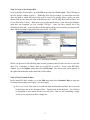
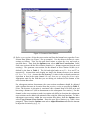
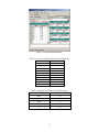
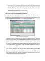
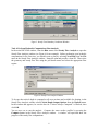
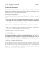
CE 3620: Water Resources Engineering
Fall 2015
Problem Set G: #5.34
Due Date: Friday October 30, 2015
Problem 5.34 from Wurbs & James is to be completed using two methods: (1) Direct-Step
Method, and (2) Standard Step Method using HEC-RAS. Additional details/requirements to
document your solution for each approach are indicated below.
Problem 5.34: Direct-Step Method
To receive full credit for your direct-step solution of Problem 5.34, at minimum, you should
provide:
(1) A plot of your water surface profile including normal depth and critical depth. (See examples
in the handout from lecture corresponding to our discussion of the direct-step method from
lecture.) Please note that a plot of water depth versus distance moved in the channel without
accounting for the elevation of the channel bottom is sufficient.
(2) Computations of normal depth and critical depth and selected type of water surface profile.
(3) Table showing solution with columns as discussed in class. You should be able to print your
entire table on 1 or 2 pages depending on your choice of step size.
(4) Sample calculations for at least one row of the table.
Problem 5.34: HEC-RAS
Instructions for HEC-RAS are provided below, as well as required output to turn in to document
your solution. This assignment is intended to help students learn how to use HEC-RAS to (1)
start a new project, (2) create a geometric file, (3) run a steady flow simulation, and (4) view the
results. This is merely a quick introduction to the HEC-RAS software. For additional information
related to open channel flow modeling and the use of HEC-RAS, students are encouraged to take
CE 4620: River & Floodplain Modeling in the fall.
The following tasks will lead you through creating a geometry file, entering and saving steady
flow data and boundary conditions, computing the water surface profile along the channel reach,
and examining the output. To get started, open HEC-RAS. HEC-RAS is installed in Dillman
computer labs. You can also download the software for free or view the user’s manual via:
http://www.hec.usace.army.mil/software/hec-ras/index.html.
Task 1: Create a New Project File
In the main HEC-RAS window, go to the File menu and select New Project. This will bring up
the New Project window (Figure 1). Within the New Project window, you must first select the
drive and path in which the project files will be stored. (To actually select a path, you must
double click the directory you want in the directory box. NOTE: HEC-RAS will not allow you
to save files to the C drive). Then enter a project title and file name. Note: the project filename
must have the extension .prj (for example, PSG.prj). Once you have entered all of the
information, click OK. A message box will then appear asking you to confirm your project title
name and the location for the project file to be saved. Click OK.
Figure 1: New Project Window.
Before you proceed to the following tasks to enter geometric and flow data, be sure to select the
units (U.S. Customary or Metric) that you would like to work in. In the main HEC-RAS
window, go to the Options menu and select Unit System. The current unit system appears to
the right of the button bar in the main HEC-RAS window.
Task 2: Enter Geometric Data
In the main HEC-RAS window, go to the Edit menu and select Geometric Data to open the
Geometric Data window (see Figure 2 for an example).
(1) Draw river reach: Select the river reach tool from the button bar and draw the river reach
by drawing a line in the direction of flow. Double-click at the end point. You will then
be prompted to enter names for the river and reach. Here we are considering a single
reach, so you only need to draw a single line.
2
Figure 2: Geometric Data Window.
(2) Define cross-sections: Select the cross-section tool from the button bar to open the CrossSection Data Editor (see Figure 3 for an example). Use the editor to define six crosssections as follows. First, use the pull down menus to select the river and reach as
specified above. Then, from the Options menu, select Add New Cross-Section. Label
each cross-section with the River Station location (i.e., distance upstream from the road
crossing). The upstream cross-section for the channel at River Station 10,000 (m) is
defined by the data in Table 1. The left and right banks are at X = 0 m and 27 m,
respectively. Assume that reach lengths are simply the distance between river stations
(i.e. Llob = Lch = Lrob). Assume that the Manning’s n values in the overbank portions are
equivalent to that in the main channel. Be sure that you are using the correct units.
Appropriate units for the field that you are editing are indicated at the bottom of the
cross-section data editor.
For subsequent stations downstream, the cross-section coordinates should be adjusted
with a uniform decrease in elevation from the previous section as specified in Table 2.
[Note: The decrease in elevation is consistent with a channel slope of 0.0005 m/m and
traversing a distance of 2,000 m downstream to the subsequent river station.] For this
channel, as the cross-sections at each river station only differ in elevation, the subsequent
cross-sections can be added with minimal effort using the following functions. To add a
subsequent cross-section, within the cross-section data editor, from the Options menu
select Copy Current Cross Section. Enter the new River Station (e.g., 8000) when
prompted. Then, from the Options menu select Adjust Elevations and enter the amount
to adjust the elevation by (e.g., -1).
3
Figure 3: Cross-Section Data Editor.
Table 1: Cross-Section Data at River Station 10000 (m)
X (m)
0
3
6
9
12
15
18
21
24
27
Elevation (m)
111.0
109.5
108.0
106.5
105.0
105.0
106.5
108.0
109.5
111.0
Table 2: Subsequent Cross-Section and Elevations
River Station (m)
Decrease in Elevation (m)
8000
1.0
6000
1.0
4000
1.0
2000
1.0
0
1.0
4
(3) Save Geometry File: You must save the Geometry file once you are finished entering the
cross-section data. In the main Geometric Data window, from the File menu select Save
Geometry Data As… Enter a title for the geometry data file. NOTE: You are only
required to enter a title, a file name is automatically established based on your project
filename and has the extension .g (for example, PSG.g).
Task 3: Enter Steady Flow Data and Boundary Conditions
In the main HEC-RAS window, from the Edit menu select Steady Flow Data to open the
Steady Flow Data window (see Figure 4 for an example). You will create a file with only one
flow profile (i.e., PF1) corresponding to the flow rate specified in the problem statement. The
flow in a reach is specified at the upstream cross-section (i.e., River Station 10000).
Figure 4: Steady Flow Data Window.
In addition to flows, a complete flow file contains the boundary conditions. Within the
Steady Flow Data window, click on Reach Boundary Conditions to open the Steady Flow
Boundary Conditions window (see Figure 5 for an example). For this problem, the flow
regime is to be simulated as subcritical, therefore, a downstream boundary condition needs to
be specified. For this problem, the boundary condition is the known (or initial) water surface
at the road crossing (i.e., River Station 0). Note: The boundary condition to be specified is
the water surface elevation. Be sure to use the correct units. To enter the water surface
elevation, click on Known WS.
Once you have entered in the given flow rate and the boundary condition, click on Apply
Data in the Steady Flow Data window. Then, save the flow data file by selecting Save Flow
Data As… from the File menu. Enter a title for the steady flow data file. NOTE: You are
only required to enter a title, a file name is automatically established based on your project
filename and has the extension .f (for example, PSG.f).
5
Figure 5: Steady Flow Boundary Conditions Window.
Task 4: Perform Hydraulic Computations (Run Analysis)
In the main HEC-RAS window, from the Run menu select Steady Flow Analysis to open the
Steady Flow Analysis window (see Figure 6 for an example). Before performing your hydraulic
computations for the first time, you should create a plan by selecting New Plan from the File
menu in the Steady Flow Analysis window. Name the plan and provide a short ID. Then select
the geometry and steady flow files using the pull down menus and select the appropriate flow
regime.
Figure 6: Steady Flow Analysis Window.
To be sure that critical depth is computed at all cross-sections and available for plotting, in the
Steady Flow Analysis window select Critical Depth Output Options from the Options menu.
In the window that appears, be sure the box for “Critical Always Computed” is checked, then
click OK.
You are now set to run the analysis. Compute the water surface profiles by pressing the
Compute button in the Steady Flow Analysis window. A window will open and show the
progress of the steady flow computations.
6
Task 5: View Output
Create a profile plot: In the main HEC-RAS window, from the View menu select Water Surface
Profiles. In the profile plot window, from the Options menu select Variables. In the window
that appears, be sure to select “Water Surface” and “Critical Depth Elevation”. Click OK to plot
these variables on the profile plot.
Create cross-section plots: In the main HEC-RAS window, from the View menu select CrossSections. The pull down menus can be used to select the cross-section for a given River Station
in the appropriate River and Reach. In the cross-section plot window, from the Options menu
select Variables. In the window that appears, be sure to select “Water Surface”, “Critical
Depth”, and “Mannings n”. Click OK to plot these variables on the cross-section.
Create a profile summary table: In the main HEC-RAS window, from the View menu select
Profile Summary Table… In the Profile Output Table window, from the Std. Tables menu
select Standard Table 1.
Please turn in the following materials to document your solution using HEC-RAS:
• River reach schematic created using HEC-RAS. Schematic should include all crosssections defined along the river reach.
• Profile plot showing the water surface elevation and critical depth for the length of the
river reach.
• Cross-section plots for stations 10,000 and 0. Each plot should show the water surface,
critical depth, and Mannings n.
• Profile summary table (Standard Table 1 format). In addition, using the results in the table
and your understanding of open channel flow from lecture:
o Explain how the top width of the water surface changes with flow depth.
o Show a sample calculation of the Froude Number at River Station 4000 (m).
NOTE: Under the File menu in each plot/table window, you can select to copy the plot/table to
the clipboard. You could then compile your answers in a single document, e.g. Word, instead of
printing everything separately.
7