Download XRADIA microXCT Manual

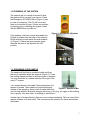
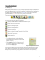
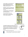
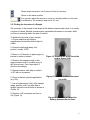
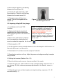
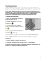
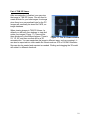
XRADIA microXCT Manual
Multiscale CT Lab
Table of Contents
1. Introduction and Basics
1.1 Instrument Parts
1.2 Powering up the system
1.3 Preparing your sample
2. TXM Controller
2.1 Starting up
2.2 Finding the Isocenter
2.3 Capturing a Single 2D X-ray Image
2.4 Acquisition of Tomographic Projections
3. TXM Reconstructor14
3.1 Doing a 3D reconstruction
4. TXM 3D Viewer 16
1
Part 1: INTRODUCTION AND BASICS
The Xradia microXCT scanner is a system that has many applications for imaging in a
variety of fields such as biology, geology, and materials science. This scanner provides
resolution up to 500 nm. The main components of the cabinet are explained in Section
1.1. This manual is intended as a brief overview how to use the micro CT and its
components. For further instructions, please consult the full 100+ page User Manual
from Xradia. The Appendix is available for extra tips. It explains how to use other
features and export files.
There are three different programs that you will be using to do imaging. These are
explained in detail sections 2, 3, and 4.
• TXM Controller – for acquisition of X-ray images from the micro CT. (Section 2)
• TXM Reconstructor - for reconstructing an aligned 2D data set. (Section 3)
• TXM 3D Viewer – Reconstructed images can be viewed as a 3D volume and exported
in different formats. (Section 4)
1.1: INSTRUMENT PARTS
1. Signal Tower – Indicates status of the Xray system. Green means power on, yellow
means the door is closed properly, and red
means X-ray is on.
2. Interior Camera Display – To view inside
the machine when the cabinet is shut and
the X-ray is ON.
Figure 1: Micro CT lab setup
3. PC interface – For all controls, i.e.
activations of x-ray source, movement of
components, etc.
4. X-ray Source
+Z
+X
+Y
5. Objectives – There are five objectives of
optical magnification; four fine objectives
(2x, 4x, 10x, 20x) on the left of the detector
and a 0.5x on the right.
6. Detector (CCD)
Figure 2: Interior scanner configuration
7. Sample Stage – Sample to be secured
on here (Details in Section 1.3).
NOTE: Axis orientation marked in Figure 2.
2
1.2 POWERING UP THE SYSTEM
The scanner will not usually be turned off and
the system will be on when you come in. Press
the Emergency Off (EMO) button (Figure 3) only
in case of emergency. The PC will be on and
there is no account to login. If there is a problem
in powering up (or resetting) the system, check
that the EMO button is pulled out.
Figure 3: Emergency off button
If the problem continues, check the breaker box
(Figure 4) located near the base of the scanner,
flip all switches up and switch the main breaker
on Figure 5. If there has been a power surge
then this will need to be flipped to the ON
position.
Figure 4: Breaker box
Figure 5: Main breaker
1.3: PREPARING YOUR SAMPLE
The sample will be fitted in a sample holder and then
placed on a platform within the scanner (Figure 6). There
are multiple sample holders for different types of samples.
You may find them in a cabinet directly to the right of the
micro CT system.
Your sample needs to be stable. During acquisition, the
sample is rotated. There should not be morphological
Figure 6: Sample holder
change of the sample or there is risk of image distortion,
such as ring artifacts. Biological samples are prone to this (e.g. an organ or limb shifting
due to gravity. Use wax, foam, or padding to immobilize it.
Another type of image distortion that can occur is beam hardening. This can occur if the
sample contains or is near metal. This occurs since the metal is too dense and reflects
the beams.
3
Part 2: TXM CONTROLLER
2.1: Starting up
When starting TXM Controller, an ‘error’ message will appear asking to recalibrate the
axis. Select yes and wait for it to finish the process. If everything is good, a dialog box
will appear and all messages will appear in a blue font. If there are any problems,
messages appear in red font. If this occurs, contact the coordinator.
There are several icons located at the top of the window:
Figure 7: Icon Toolbar
The main ones being uses will be the following:
Displays available XRM and TXRM files available to open
Saves a file onto the hard drive
Opens the settings window
Starts an image acquisition
Aborts an acquisition
Opens or closes the Image Properties Control Panel
Adjusts the X-ray source
Begins acquisition
•
The voltage and power can be adjusted as
needed based on the material or object being
imaged. (Figure 8)
•
Clicking apply will turn the X-ray source on. If
you make any adjustments to these settings,
you must click apply again.
Figure 8: X-ray Source window
There are three different scan modes primarily used and are selected from the gear
menu. Each can be adjusted for time of exposure and number of binnings needed.
Binning is the procedure for grouping data into data classes for later processing.
4
Continuous Mode – Used for setting up the
scans and adjusting movement of the
sample. This mode takes short, coarse
images continuously. Also be accessed by
clicking the video camera icon.
Single Mode – Gives you one quality image,
similar to a regular X-ray taken if you broke
your arm. Clicking the camera icon can also
access this.
Tomography Mode – This mode will ‘slice’
the sample and produce a 3D image that
can be manipulated later.
Figure 9: Acquisition mode window
There are three tabs for the motion
controller (Figure 10). This moves the
detector, source, and sample during the
course of taking an acquisition.
Figure 10: Motion controller window
To manipulate the sample into the path of the source, use
the joystick to move the sample or motion controller buttons
(Figure 10). There are three degrees of spatial freedom for
moving the sample in the XYZ directions. The angle Ø will
rotate the sample. To move the stage up, you must go in
the negative Y direction. For further axis orientation, see
Figure 11.
+Z
+X
+Y
Figure 11: Axis
orientation
Using following icons can move the source:
Moves toward sample +Z at given step size in millimeters
Moves away sample –Z at given step size in millimeters
5
Pause stops movement, use if unsure of how it is moving
Return to the home position
You can also select the source to move to a certain position on the track
in millimeters. The minimum step size is 0.1 mm.
2.2: Finding the Isocenter of a Sample
The isocenter of the sample is the where all the beams intersect each other. It is usually
a region of interest. Medical scanners have a predefined isocenter for the scan, while
you have to manually define the axis of rotation.
To define the isocenter of your sample:
1. Choose objective with highest
magnification at which the entire object is
visible.
2. Rotate a small angle away from
position, usually 10-20º.
3. Move in +/-Z direction to place region of
interest in center of screen.
Figure 12: Drawing the initial line at the
unique aspect (UA)
4. Rotate to the negative angle of the
angle chosen in step 2 to make sure it is
still in the screen. If not, then adjust Z
direction accordingly.
5. Repeat rotations until able to rotate to
+/-90º with no movement.
6. Zoom to desired optical magnification
(e.g. 20x)
Figure 13: Post-90º rotation, draw new
line at UA
7. Use a unique aspect (UA) of the sample
(edge, particle, tooth, etc) and draw a
straight vertical line at this site as shown in
(Figure 12).
8. Rotate to +90º and place new line on
UA (Figure 13).
Figure 14: Move UA in Z direction
halfway between the two lines
6
9. Move sample Z direction until halfway
between two lines (Figure 14).
10. Remark UA and rotate back to -90º
Move sample in Z direction until halfway
between two lines and remark UA.
11. Repeat process until there is no
change. The two lines appear as one
(Figure 15).
Figure 15: Final position of object, the
two lines appear as one
2.3: Capturing a Single 2D X-ray Image
1. Load Sample and launch TXM
Controller
2. Adjust optical objective to desired
magnification by selecting Microscope
then Configure systems on the menu and
select OK.
• Note: It is important to get the detector
as close as possible to the sample. Be
sure to view with the interior camera. IF
YOU ARE NOT CAREFUL YOU MAY
CRASH THE SCANNER!!!
• Move the detector back, change the
objective, and then move to the previous
position. Pausing or stopping all motors
can be used.
3. Move source and detector to farthest
limit from sample by selecting the limit
arrow icon under the respective tab for each.
4. Rotate sample to -90º.
5. Use the joystick or motion controller buttons to move the sample in XYZ directions to
the center and zoom in on the monitor.
6. Rotate back to 0º and then move the sample in Z direction.
7. Close the door and turn on X-ray. Adjust the power and voltage according to sample
being scanned.
8. Defining the isocenter (Details in Sec. 2.2)
9. Move the detector and source as close as possible to the sample.
10. Select the gear icon, select continuous mode (example settings: exposure time = 1
sec, binning = 4). After, make any necessary adjustments to the detector, source, or
sample.
11. Select the gear icon and select single mode (typical settings: exposure = 20 - 60
seconds, binning = 1).
7
12. Click the disk icon to save image acquired.
2.4: Acquisition of Tomographic Projections
***This section will be used the most by the majority of micro CT users***
2.4: ACQUISITION OF TOMOGRAPHIC PROJECTIONS
***This section will be used the most by the majority of micro CT users***
1. Mount prepared sample inside scanner using three-point mount.
2. Position sample in correct XYZ location. With the door open, move the sample in the
XYZ directions until it is positioned in the X-ray beam line.
3. Verify the sample will not hit the source or detector during rotation. Move the source and
detector to the positions needed. Make sure that source or detector won’t collide with the
sample in a full +/- 90º rotation.
4. Close the enclosure door (signal tower yellow light on)
5. Activate the X-ray source (Sec. 2.1)
6. Begin Acquisition (example settings: Exposure = 1 second, binning = 4x4) (Sec. 2.1).
Move the sample to the desired position in the X and Y directions (Sec 2.2).
7. Position sample in rotation axis in Z (beam line) direction (Sec. 2.3)
8. Select the gear icon, select Tomography mode (Sec. 2.1), and set exposure time,
binning, and readout time (Typically: 60 seconds, 1x1, and fast). Set starting angle, end
angle, and number of images to be acquired (Typically +90, -90, and 721).
9. Begin acquisition. There is a prompt to choose a filename and location for the acquisition
file. Name the file according to the naming convention. This naming convention is for the
folder only. *
10. The status of the acquisition will be updated with how many hours the scan will take
and the memory required. After a scan begins, it will take several hours to complete. The
X-ray will shut off automatically.
* For storing images, the naming convention for folders is: PIName_YYYY_MM_DD_Initials.
Example:
For Mr. John Smith working on a project under Dr. Bob Prado on June 23, 2009, the folder
name will be Prado_2009_06_23_JS
8
Part 3: TXM Reconstructor
Use the TXM Reconstructor program to assemble your images into a usable format.
There are various ways to adjust your images for better quality. One way is final center
shift if your scan is off axis and this will shift the scans. Correction to the beam line can
also be made if needed. Reconstruction time will vary based on number of projections
and settings used. TXM 3D Viewer can be used to view the volume and cross-sectioned
slices. If the scanned sample was weak absorbing object, use phase contrast in
reconstruction. Phase contrast relies on the refractive properties of the object.
3.1: Doing a 3D reconstruction
1. Launch TXM Reconstructor and open the
desired tomography data set.
2. Select the Reconstruction Icon to start
reconstruction. [
]
3. Find the rotation center if needed by
clicking on the rotation center icon in the tool
bar. [
]
4. Click on the reconstruction settings icon in
the toolbar. [
Figure 16: Reconstruction settings
window
] (Figure 16)
5. Select a file name and path to store the 3D volume in the Output File Name box.
6. Click the PreProcess button to perform the preprocessing before starting the
reconstruction.
7. Select the OK button to begin the reconstruction.
8. The program will now reconstruct the data set into a 3D volume data set.
9. When the reconstruction is finished, a completion message will be displayed with the
amount of time required to complete the reconstruction.
9
Part 4: TXM 3D Viewer
After reconstruction is finished, you may view
the image in TXM 3D Viewer. You will need to
create a folder for your labs images for storage
since there is no personalized login for the PC.
Images will eventually be stored on PACS, an
image database.
When viewing images in TXM 3D Viewer, by
default you will have four windows to view and
rotate your images (Figure 17). There will be
three windows to view different planes. There is
Figure 17: The 3D Viewer window
XY, YZ, XZ, and then one that will be a 3D
reconstruction. You can manipulate the image in different ways, such as cropping it. It
can also be exported into other usable file formats such as JPG or DICOM. Animation
files can also be created and exported as needed. Clicking and dragging the 3D model
will rotate it in different directions.
10