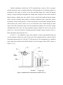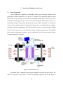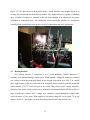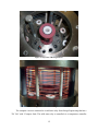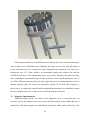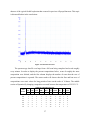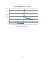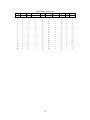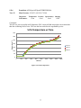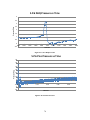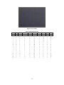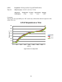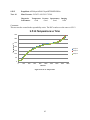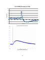
1
SOLID PROPELLANT SLOW COOKOFF EXPERIMENTS WITH ADVANCED DIAGNOSTICS BY BRADLEY J. HORN THESIS Submitted in partial fulfillment of the requirements for the degree of Master of Science in Mechanical Engineering in the Graduate College of the University of Illinois at Urbana-Champaign, 2011 Urbana, Illinois Advisor: Professor Nick Glumac Abstract Slow cookoff of solid propellant was experimentally studied at the University of Illinois by examining the behavior throughout the cookoff process. The general concept involved preparing axial-symmetric samples of chosen compositions and casting them into carbon fiber cases. The cured samples were then placed inside the test apparatus to slowly heat until auto-ignition while continuously recording data used to help validate a complex thermal-chemical-mechanical code being built to model the cookoff behavior of energetic materials. Preliminary work focused on developing the test apparatus and successful implementation of all diagnostics. Experimental data taken for the scope of this research included three thermocouple readings of varying radius for spatial temperature gradients, pressure and spectrometry measurements on decomposition and combustion gases, and images of the surface of the carbon fiber case used in digital image correlation to yield mechanical displacement. Single base ammonium nitrate propellant was the first propellant composition used in developing the test apparatus. Following successful implementation and testing of the diagnostics, a series of tests were conducted to establish repeatability of all developed methods and procedures. For these tests, a common ammonium perchlorate composition previously used was duplicated to compare the data [14]. After successful repeatability tests, single-base propellants were tested in accordance with slow cookoff standards. The development of the test apparatus, results of all tests, and current status of all diagnostics are discussed in detail. II Dedication This thesis is dedicated to my family and friends: to my parents Guy and Barb Horn for always encouraging me throughout my education to do my best and for being proud of me no matter the outcome; to my brothers Corey and Rob for always being there for me and serving as role models throughout my life; to my entire family whom I love with all my heart; without you I would be lost and without direction. III Acknowledgements I wish to thank Prof. Nick Glumac and Prof. Herman Krier for all their guidance and wisdom throughout my studies. Prof. Krier said, “If we knew of what we were doing, they wouldn’t call it research.” I now appreciate the process of research and without your guidance I could not have completed that journey. Thank you. I would also like to thank my past and present research group including David Allen, David Chonowski, Michael Clemenson, Drew Coverdill, David Joyce, Joe Kalman, Lance Kingston, Patrick Lynch, Jeffrey Mason, Jennifer Peuker, and John Rudolphi. Thank you for all your wisdom and help. It has been a pleasure working with all of you. Cheers to you all! Special thanks to my research-assistant Mark Janowski who was involved in nearly all aspects of my research. Another special thanks to Julio Barros for helping with the digital image correlation code. Special thanks to Andy Tudor for the help and instruction in image processing of scanned propellants. I would also like to thank my friend and fellow student Mark Shoemaker. This journey was made easier by having a friend along the way. My last acknowledgment is to my undergraduate physics professor and advisor Dr. Christopher Fasano. Words cannot express my sincerest gratitude for your diligent mentoring and guidance. Everything that I have achieved through undergrad and graduate studies has been a direct result of your encouragement. Thank you very much. The work in this thesis covers the experimental portion of a collaboration between IllinoisRocstar, Notre Dame, and the University of Illinois supported by the United States Army, project number W31P4Q-11-C0076: Experimental and Computational Program for Slow and Fast Cookoff for Insensitive Munitions Testing. IV Table of Contents List of Figures ............................................................................................................................... VI List of Tables ............................................................................................................................. VIII List of Terms and Symbols ........................................................................................................... IX 1 Introduction ............................................................................................................................. 1 1.1 Solid Propellant .................................................................................................................1 1.2 Slow Cookoff Fundamentals .............................................................................................2 1.3 Literature Review ..............................................................................................................5 1.4 Problem Statement ............................................................................................................8 2 Experimental Equipment and Process ................................................................................... 10 2.1 General Apparatus ...........................................................................................................10 2.2 Heating Element ..............................................................................................................11 2.3 Diagnostics ......................................................................................................................13 2.3.1 2.3.2 2.3.3 2.3.4 Temperature ............................................................................................................................ 14 Pressure ................................................................................................................................... 15 Imaging ................................................................................................................................... 16 Spectroscopy ........................................................................................................................... 17 2.4 Optical Absorption ..........................................................................................................18 2.5 Propellant Preparation .....................................................................................................20 3 Preliminary Work .................................................................................................................. 22 3.1 Original Apparatus ..........................................................................................................22 3.2 Heating Element Versions ...............................................................................................22 3.3 Diagnostic Implementation .............................................................................................24 3.4 LabView Programming ...................................................................................................27 3.5 Initial Test Results ...........................................................................................................28 4 AP Propellant Results and Discussion .................................................................................. 31 4.1 Repeatability Results .......................................................................................................31 4.2 Slow Cookoff Results......................................................................................................35 5 Conclusion and Recommendations ....................................................................................... 40 5.1 Conclusion.......................................................................................................................40 5.2 Recommendations ...........................................................................................................42 List of References ......................................................................................................................... 44 Appendix ....................................................................................................................................... 46 A. Typical Ingredients of Composite Solid Propellants ......................................................... 46 B. LabView Design................................................................................................................. 47 C. Data Analysis Procedure .................................................................................................... 49 D. Solid Propellant Slow Cook-off Standard Operating Procedure ....................................... 54 E. Time, Expenses, & Parts List ............................................................................................. 61 F. Cookoff Data ...................................................................................................................... 63 G. CEA Results ....................................................................................................................... 89 H. Data Processing Codes ....................................................................................................... 93 V List of Figures Figure 1.1 Stages of Cookoff [11] .................................................................................................. 4 Figure 1.2 Thermal Runaway Physics [11]..................................................................................... 4 Figure 1.3 VCCT Finite Element Mesh *Taken Directly from Reference [23] ............................. 6 Figure 1.4 Modified SSCB *Taken Directly from Reference [13] ................................................. 7 Figure 2.1 General Schematic [11] ............................................................................................... 10 Figure 2.2 Entire Apparatus Inside Sound Enclosure ................................................................... 11 Figure 2.3 Top View of Heating Element ..................................................................................... 12 Figure 2.4 Side View of Heating Element .................................................................................... 12 Figure 2.5 Solid State Relay ......................................................................................................... 13 Figure 2.6 Temperature Controller ............................................................................................... 13 Figure 2.7 T-Couple Placement Schematic .................................................................................. 14 Figure 2.8 TCIC 8 Channel Thermocouple Card.......................................................................... 15 Figure 2.9 Gems Pressure Sensor ................................................................................................. 15 Figure 2.10 Gems Pressure Sensor & Gas Filter .......................................................................... 15 Figure 2.11 NI USB-6008 DAQ Card .......................................................................................... 16 Figure 2.12 CCD Camera and Shielding ...................................................................................... 17 Figure 2.13 CCD Camera 0.5 mm Markings ................................................................................ 17 Figure 2.14 SRS 200 Quadrupole Mass Spectrometer ................................................................. 18 Figure 2.15 IR Optical Absorption Diagram ................................................................................ 19 Figure 2.16 Propellant Slurry........................................................................................................ 20 Figure 2.17 Propellant Casted in Stand......................................................................................... 20 Figure 3.1 Original Experimental Setup ....................................................................................... 22 Figure 3.2 View Without Heat Shield........................................................................................... 22 Figure 3.3 Heating Element Version II ......................................................................................... 23 Figure 3.4 View of Setup (Version II) .......................................................................................... 23 Figure 3.5 Heating Element Version III Schematic ...................................................................... 24 Figure 3.6 Teflon .......................................................................................................................... 26 Figure 3.7 Expanded Teflon with DIC ......................................................................................... 27 Figure 3.8 CCD Image of S.P.2 .................................................................................................... 29 Figure 3.9 CCD Image of S.P.25 .................................................................................................. 29 Figure 3.10 S.P.1 Data (AN) ......................................................................................................... 30 Figure 4.1 Repeatability R=3/3 Temperature Plot ........................................................................ 34 Figure 4.2 Repeatability DAQ Pressure Plot ................................................................................ 35 Figure 4.3 S.P.25 Temperature ..................................................................................................... 36 Figure 4.4 S.P.25 Pico Pressure .................................................................................................... 37 Figure 4.5 S.P.25 at 25 ℃ ............................................................................................................. 39 Figure 4.6 S.P.25 at 75 ℃ ............................................................................................................. 39 Figure B.1 Cookoff Control VI Front Panel ................................................................................. 47 Figure B.2 Cookoff Control VI Block Diagram ........................................................................... 48 Figure C.1 Amira S.P. Image Processing ..................................................................................... 50 Figure C.2 Amira Particles ........................................................................................................... 53 Figure F.1 S.P.1.3.2 Temperature ................................................................................................. 63 Figure F.2 S.P.1.3.2 DAQ Pressure .............................................................................................. 64 Figure F.3 S.P.2 Temperature ....................................................................................................... 65 VI Figure F.4 S.P.3 Temperature ....................................................................................................... 66 Figure F.5 S.P.3 DIC..................................................................................................................... 66 Figure F.6 S.P.4 Temperature ....................................................................................................... 67 Figure F.7 S.P.4 DAQ Pressure .................................................................................................... 68 Figure F.8 S.P.4 DIC..................................................................................................................... 68 Figure F.9 S.P.10 Temperature ..................................................................................................... 69 Figure F.10 S.P.10 DIC................................................................................................................. 69 Figure F.11 S.P.9 Temperature ..................................................................................................... 71 Figure F.12 S.P.8 Temperature ..................................................................................................... 73 Figure F.13 S.P.8 DAQ Pressure .................................................................................................. 74 Figure F.14 S.P.7 Temperature ..................................................................................................... 75 Figure F.15 S.P.7 DIC................................................................................................................... 75 Figure F.16 S.P.6 Temperature ..................................................................................................... 77 Figure F.17 S.P.6 DAQ Pressure .................................................................................................. 78 Figure F.18 S.P.6 Pico Pressure .................................................................................................... 78 Figure F.19 S.P.6 DIC................................................................................................................... 79 Figure F.20 S.P.12 Temperature ................................................................................................... 80 Figure F.21 S.P.12 DAQ Pressure ................................................................................................ 81 Figure F.22 S.P.12 Pico Pressure .................................................................................................. 81 Figure F.23 S.P.12 DIC................................................................................................................. 82 Figure F.24 S.P.13 Temperature ................................................................................................... 83 Figure F.25 S.P.13 DAQ Pressure ................................................................................................ 84 Figure F.26 S.P.13 Pico Pressure .................................................................................................. 84 Figure F.27 S.P.13 DIC................................................................................................................. 85 Figure F.28 S.P.14 Temperature ................................................................................................... 86 Figure F.29 S.P.14 DAQ Pressure ................................................................................................ 87 Figure F.30 S.P.14 Pico Pressure .................................................................................................. 87 Figure F.31 S.P.14 DIC................................................................................................................. 88 VII List of Tables Table 3-1 Preliminary Tests Overview ......................................................................................... 29 Table 4-1 Repeatability Test Overview ........................................................................................ 31 Table 4-2 Temperature Standard Deviations in Degrees Celsius ................................................. 32 Table 4-3 Temperature Percent Differences ................................................................................. 32 Table 4-4 Pressure Standard Deviations in Psi ............................................................................. 32 Table 4-5 Spectroscopy Standard Deviations in Percent Compositions ....................................... 33 Table 4-6 Cookoff Response of Modified SSCB AP/HTPB (88/12) Propellant [13] .................. 34 Table 4-7 S.P.25 Slow Cookoff Overview ................................................................................... 36 Table 4-8 S.P.25 Spectroscopy ..................................................................................................... 37 Table E-1 Time Table & Expense Summary ................................................................................ 61 Table E-2 Parts List ...................................................................................................................... 62 Table F-1 S.P.10 Spectroscopy ..................................................................................................... 70 Table F-2 S.P.9 Spectroscopy ....................................................................................................... 72 Table F-3 S.P.8 Spectroscopy ....................................................................................................... 74 Table F-4 S.P.7 Spectroscopy ....................................................................................................... 76 Table F-5 S.P.6 Spectroscopy ....................................................................................................... 79 Table F-6 S.P.12 Spectroscopy ..................................................................................................... 82 Table F-7 S.P.13 Spectroscopy ..................................................................................................... 85 Table F-8 S.P.14 Spectroscopy ..................................................................................................... 88 VIII List of Terms and Symbols Al Aluminum AN Ammonium Nitrate (oxidizer) AP Ammonium Perchlorate (oxidizer) DIC Digital Image Correlation DOA Dioctyle Adipate (plasticizer) HCl Hydrochloric Acid HTPB Hydroxyl-Terminated Polybutadiene (binder) IM Insensitive Munitions IPDI Isophorone Diisocyanate (curing agent) IPSTP Insensitive Propellant Screening Test Protocol Material Density QMS Quadrupole Mass Spectrometer SNL Sandia National Laboratories SOP Standard Operating Procedure S.P. Solid Propellant SSCB Super Small-Scale Cookoff Bomb T Temperature t Time VCCT Variable Confinement Cookoff Test VI Virtual Instrument (LabView) IX 1 Introduction The earliest recorded use of propulsion is attributed to a Greek named Archytas in 400 BC where steam was used to propel a wooden bird in flight [7]. Two hundred years later the concept of solid propellant originated when the Chinese developed black powder for entertainment and eventually warfare. Their version of today’s black powder was a simple mixture of charcoal, sulfur, and rock salt. The Chinese started using the compound in religious and funeral activities by filling bamboo sticks, sealing them, and throwing them into a fire to produce explosions. It is believed that some of these were improperly sealed allowing the first version of rockets to propel out of the fires. Over the next thousand years, the Chinese developed the concept into “fire arrows” that are first recorded as being used for weapons against Mongol invaders in the battle of Kai-fung-fu in 1232 A.D. [7] Over the next five hundred years the use of rockets in warfare spread from the Mongols to the Arabs, French, and later the British. The applications of solid propellant and rockets went in waves, varying in use between warfare and entertainment. During these years, small improvements were made including improved powder for sustained burn time, tubular launch design, and multistage rockets. However, little improvements were made to the accuracy of rockets whose effectiveness relied on sheer numbers. The first presence of rockets in America was during the Battle of 1812 and led to “the rockets’ red glare,” in the Star Spangled Banner. By the early 1900’s scientists from Germany, Russia, and the United States were exploring the advancement of rockets and soon turned to the use of liquid propellant. Goddard in the U.S. was the first to use liquid fuel and was soon followed by von Braun in Germany during WWII. On October 4, 1957 Sputnik was launched spurring the space race between the Soviet Union and the United States. [7] 1.1 Solid Propellant Solid propellant is comprised mainly of fuel and oxidizer that, when ignited, rapidly produces a large amount of hot gas. By mixing an oxidizer into the composition, the propellant is able to combust without the presence of external oxygen from the atmosphere. If contained, the rapid production of pressure can build, until mechanical failure of the confinement yielding an explosion. When allowed to vent through a nozzle, the release of hot gases are directed to 1 produce thrust, powering a rocket into motion. Once ignited, solid propellant is extremely difficult to extinguish without a rapid depressurization. Solid propellant is categorized as composite or either a single-base, double-base, or triplebase. Double-base propellant contains fuel and oxidizer chemically mixed to form a homogenous substance usually consisting of nitroglycerine and nitrocellulose. Commonly the propellant is found in a powder grain or crystal form that can be combined with other additives and a plasticizer to form a heterogeneous composite mixture with desired attributes. Single-base propellants generally consist of a powder oxidizer mixed with a binder for fuel that forms a heterogeneous composite mixture with other additives to change the properties. Common oxidizers used for rockets include ammonium perchlorate NH4ClO4 (AP), ammonium nitrate NH4NO3 (AN), potassium perchlorate KClO4 (KP), and potassium nitrate KNO3 (KN) [14]. In single-base compositions the rubber binder, commonly hydroxyl-terminated polybutadiene C7.332H10.982O0.058 (HTPB), is the main source of fuel and serves to hold the granular mixture together. Plasticizers help in the elongation of the mixture during processing and dioctyle adipate C22H42O4 (DOA) is a common choice. A small percentage of mass can be additional curing agents like isophorone diisocyanate C12H18N2O2 (IPDI) to help solidify the binder [15]. [See Appendix A for a detailed list of common ingredients [14].] Additional materials can be added to improve or modify material characteristics or combustion performance. Metal additives such as aluminum (Al), boron (B), or magnesium (Mg) are used to add additional energy to the combustion process. However, metal additives add instability and an increased danger when manufacturing and handling. During the past century due to the military, NASA, and small rocket enthusiasts, significant research has been conducted on various compositions and materials down to the effect of geometrical configuration of the grains. 1.2 Slow Cookoff Fundamentals Cookoff refers to the process of heating an energetic material until it reaches self or auto- ignition. The ignition temperature is the point when the material enters a self-sustained reaction that is an exothermic, dynamic process that will continue without external heating. Cookoff is a thermal, chemical, and mechanical complex process. There are two main categories of cookoff determined by the heating rate which are slow and fast cookoff. The division between the categories is not always well defined and depends on which source is referenced. The general 2 range is that slow cookoff is on the order of 2-6 ℃/hr, where fast cookoff is loosely defined as a fuel fire on the order of 70 ℃/hr with the distinction between the two being undefined. In work by Geisler [9], three heating rates characterized as low, medium, and high with corresponding rates of 13.8, 1200, and 90k ℃/hr. According to the slow heating NATO STANAG 4382 test, the slow cookoff heating rate is defined as 3.3 ± 0.5 ℃/hr after heating the sample at 5 ℃/min to 50 ℃ and held constant for 8 hours for thermal conditioning [6]. [This standard for slow cookoff is also found in references [1], [13], [26]] Another common standard in literature and industry is 6 ℃/hr following a similar initial thermal ramp [13]. The heating rate greatly determines the ignition temperature as well as the severity of the damage. Contrary to intuition, as the heating rate is increased, the ignition temperature increases while the level of damage decreases. As a result, slow cookoff is more dangerous than fast cookoff and extensive research has been done to design composite casings that help in preventing slow cookoff conditions. Additional research has been done on modifying the composition of insensitive munitions (IM) to be less susceptible to stimuli [27] as well as slow cookoff environments. During the initial stages of heating, the physics governing the behavior of the propellant is strongly dictated by basic heat transfer and quasi-static mechanics. The first stage of cookoff is an endothermic process, represented as stage a in Figure 1.1 below. As the temperature increases thermal expansion occurs and thermal coefficients change due to the material transformation. Once the point of self-sustained reaction or thermal runaway occurs (stage b), the rate of gas pressurization increases significantly. The mechanical interaction of the propellant and pressurization within the confinement dictates the type of reaction upon ignition. For AP/HTPB propellants the cookoff becomes exothermic at about 247 ℃ [22]. 3 Figure 1.2 Thermal Runaway Physics [11] Figure 1.1 Stages of Cookoff [11] Once ignition is reached, the sample is categorized based on the speed and severity of the combustion process as deflagration, explosion, or detonation. The extensive definitions and qualifications for each category are explained in detail in the TB 700-2 regulatory document “Department of Defense Ammunition and Explosives Hazard Classification Procedures” [6]. A deflagration is a rapid moving combustion wave with a flame velocity on the order of 1-10 mm/s while an explosion also includes a pressure burst and fragmentation. A detonation event is separated from explosion by the criteria of a supersonic propagation wave which results in a severe blast effect and fragmentation. The critical diameter of AP/HTPB propellants exceed 200 mm or 7.87 inches, which is much greater than the size of the propellant samples used in this research and most in-service rocket motors eliminating possible detonations [13]. Upon ignition, the combusting propellant emits high temperature gases, increasing the pressure while transferring heat to the unburned propellant raising its temperature. As a result, a chain reaction occurring in the unburned propellant causes an exothermic chemical reaction repeating the process which creates a flame front or combustion wave. The propagation of the combustion wave is dependent on the propellant composition, structure, pressure, temperatures both initial and flame, and other variables. During the combustion, three phases exist consisting of solid (solid propellant), mixed (liquid and solid), and gas (combustion gases and premixed flame). The mixed phase region of liquid and solid is a condensed phase above which resides the hot reactive gases which form the luminous flame. [14] 4 Assuming a conventional flame structure on the surface of the propellant, the AP and HTPB decompose and form NH3 and HClO4. Oxidizing reactants form flamelets which when combined with the fuel reactants produce a diffusion flame structure. The final gas products include HCl, CO, CO2, H2O and N2. However, it is important to note that the point of ignition can occur anywhere inside or on the surface of the propellant. 1.3 Literature Review Historically, most large scale tests are performed in order to categorize energetic materials according to the industry standard TB 700-2 [6]. Typically, large scale tests have been done with fast cookoff characteristics where the damage is measured qualitatively along with possible temperature and pressure measurements as a function of radius from the object. In this manner, a large amount of literature focuses on regions of damage or the level of violence rather than the state of the material during the stages preceding ignition [3] [5] [7] [10] [21] [27]. Recently, studies have been moved to correlating between small and full scale test methods in the search to establish a reliable small scale methodology for testing and screening for materials that will not pass full scale tests. The drive for this research is to provide a small scale alternative adoptable by the TB 700-2 regulations. Full scale tests are expensive and can be dangerous. Establishing a reliable correlation between scales will allow classification of energetic materials in a cheap and efficient manner. Tests being developed are the Critical Diameter (Dc), the Burning-To-Violent Reaction, Thermal Properties Characterization (TPC), and the Critical Impact Velocity (CIV) tests [5]. The TPC test is the most relevant test designed with diagnostics to determine ignition temperatures, exotherms, endotherms, weight-loss, volume-increase, and combustion products. A separate test uses a small motor that is ignited after similar heating in order to measure pressures that reveal the affect of thermal degradation on the propellant performance. Since the 1990’s Sandia National Laboratories (SNL) have been developing a complex model to simulate the cookoff environment. First, a complex code was built to model solid propellant for defined conditions during the final stages of cookoff [3]. The code used shock physics to model the stages of cookoff between deflagration to detonation (DTD) in porous energetic materials. Results indicated that the percent porosity greatly affected the characterization of the violence of cookoff as well as the time scale of the event. The time scale from ignition to the end of the event ranged from 16-90 μs depending on the percent porosity. 5 The conclusions from the research were that a lot more understanding was needed on the state of thermally conditioned material prior to ignition in order to better understand the final stages of cookoff. Later at SNL, a finite element analysis code was developed as of August, 1994 [2]. A combination of already existing codes, COYOTE II, CHEMEQ, XCHEM-1D, and CHAPARRAL were modified to implement heat conduction and decomposition, multistep rate equations, thermal chemistry, and radiation computing respectively. According to the paper, the mechanical aspect of the problem other than simple material addition or deletion was not yet included due to limitations in finite element multidimensional solving methods. At the time of this project, computing limits were a large factor in allocating memory to finer mesh element calculations. As a result, larger elements that neglected small scale chemistry and elementrefinement methods were used. The refinement methods used in the code at that time were a new research area in computational modeling. A common experimental setup used for the study of cookoff is the variable confinement cookoff test (VCCT) used by the Naval Surface Warfare Center. Figure 1.3 is the VCCT finite element mesh used by Sandia National Laboratories [23]. Figure 1.3 VCCT Finite Element Mesh *Taken Directly from Reference [23] The SNL finite element code briefly incorporated the first stage of cookoff up to ignition temperatures by modifying the energetic material into a thermally damaged state categorized by porosity, specific surface area, and crack density. Later on, SNL incorporated JAS into the model to better account for this mechanical behavior. 6 Variable confinement cookoff tests (VCCT) predicted that as much as 10% of energetic material decomposes prior to ignition indicating a strong dependence on mechanical physics in modeling the early stages of cookoff. It was also noted that during slow cookoff the thermal damage is largely distributed throughout the sample when compared to the surface-localized thermal damage resulting from fast cookoff. In slow cookoff the distributed thermal damage allows convective burning which produces accelerated combustion and a rapid flame spread. Experiments focused on the presence of cracks and porosity in the thermally damaged material which increases the specific surface area. It was found that cracks formed during the initial stages, allow flame penetration deeper into the propellant and enhance the convective burning with higher burn rates at the crack tips. Hypotheses disagree whether the cracks or the specific surface area is the main element in dictating thermally damaged energetic material, and it is likely that neither can be neglected. [23] In 1995 S. Y. Ho published a paper that contained a similar experimental design and research elements related to the scope of this report. Ho performed both slow and fast cookoff experiments characterized as 6 ℃/hr and 72 ℃/hr respectively. The test apparatus was a modified super small-scale cookoff bomb (SSCB) defined by Naval Weapons Center (NWC) shown in Figure 1.4. [13] Figure 1.4 Modified SSCB *Taken Directly from Reference [13] 7 Ho studied the effect of percent composition of plasticizer on the reaction violence in both fast and slow cookoff. From his research Ho suggested a possible criterion in categorizing slow versus fast cookoff being the reversal of the temperature gradient, especially during thermal runaway. In fast cookoff, the hottest area is on the surface of the propellant which was 30-40 ℃ higher than the center while slow cookoff exhibited nearly uniform temperature distribution within 30 minutes. The point of ignition, surface versus center, correlates to fast versus slow heating as well as reaction violence. The reaction violence was experimentally quantified by the peak pressure, the impulse, and the initial rise (dP/dt). Ho also found that with slow heating, the HTPB/AP propellant became structurally tougher due to the oxidation of the HTPB binder and as a result exhibited higher thermal conductivity resulting in higher temperatures, more uniform thermal distribution, and more violent cookoff reaction. It should be noted that Ho performed experiments measuring angular thermal gradients and, as expected, found the variance to be insignificant and less than 3℃ throughout cookoff. [13] 1.4 Problem Statement Traditionally, cookoff is modeled with a thermal-chemical model that is decoupled from the mechanical behavior of the energetic material. Ignoring the mechanical state of the propellant allows for a good approximation during fast cookoff but induces non-negligible errors during slow cookoff. It is now understood that the thermally damaged mechanical state of the propellant favors conditions for thermal runaway and increases shock sensitivity. Previous literature [3] [5] [7] [10] [21] [27] focuses on the effects of various environments on the level of violence in cookoff by assessing the fragment size of debris resulting from confinement failure. In a paper from SNL it is noted, “These simulations strongly suggest that the determination of the thermal damage states, prior to the onset of ignition, is the key issue toward determining the degree of reaction violence associated with cookoff.” [1] The experimental work presented in this work is part of a multiphase research endeavor aimed at producing a complex chemo-thermal-mechanical model to accurately predict the behavior for various solid propellants. The experimental tests conducted serve to validate the construction and performance of the complex coupled model. Multiple diagnostics collect data to validate the temperature distribution, decomposition gases, pressure, and surface displacement. In our work, an adaptation of the VCCT and SSCB experimental setups is used 8 primarily to study the state of the energetic material from the start of heating up to the point of ignition. 9 2 2.1 Experimental Equipment and Process General Apparatus The test apparatus is designed to accommodate either cased or uncased cylindrical solid propellant of variable length from 1-2” and of 0.75” diameter. The propellant sample is seated firmly inside two spacer plates, top and bottom, that hold the sample in line with the center. Four axially-spaced bolts apply pressure to form seals. Holes through the bottom plates allow access for the thermocouples. Seated inside the top plate is a quartz window for optical access inside the annulus of the propellant sample. Seated inside the bottom plate is a polished reflective stainless steel piece with a gas sampling port. The reflective surface serves as a mirror to bounce off light from an off axis source that can be collected to perform absorption spectroscopy. The sampling port connects to the pressure transducer and the capillary tube used for the gas analysis. Figure 2.1 depicts the general schematic. Figure 2.1 General Schematic [11] The bottom plate is mounted on optical post assemblies secured to an optics board. The optics board provides a rigid surface to attach all shielding, diagnostics, and wiring shown in 10 Figure 2.2. The optics board is then placed inside a sound enclosure and strapped down to an existing structure present for unrelated experiments. The sound enclosure is capable of handling up to 15 grams of explosives. Attached to the top of the chamber is an exhaust fan for proper ventilation of combustion gases. All connections extend outside the chamber to a workstation controlled from an adjoining room for three levels of containment and safety precautions. Figure 2.2 Entire Apparatus Inside Sound Enclosure 2.2 Heating Element The heating element is comprised of 0.02” thick nichrome (Nickel-Chromium C) resistance wire threaded through ceramic posts. When applied a voltage the nichrome resistance wire radiates to heat the propellant sample to any desired temperature up to 400 ℃ at variable rates. Eight ceramic posts are positioned in an octagonal pattern centered round the propellant with a distance of 2.375” from each post to the center. This pattern creates a nearly angularlysymmetric heat source. Each ceramic post is machined with diamond-tipped drill bits to allow 8 loops of nichrome resistance wire. A single wire completes 8 loops through the ceramic tubes with a resistance of 16.6 ohms. When applied a wall outlet voltage the circuit yields 7.5 or less amperes. Figure 2.3 and Figure 2.4 show the heating element from a top and side view. 11 Figure 2.3 Top View of Heating Element Figure 2.4 Side View of Heating Element The complete circuit is connected to a solid state relay from Omega Engineering that has a 330 VAC with 25 ampere limit. The solid state relay is controlled via a temperature controller 12 that uses a 4th thermocouple as a reference signal. The thermocouple is placed at the same depth as the yellow thermocouple discussed in section 2.3.1. A software package from Omega is used to program and run the temperature controller. The temperature controller establishes a starting temperature of 25 ℃ and then ramps to 50 ℃ in 5 minutes followed by thermal conditioning for an hour at constant temperature. After which the propellant is heated at a rate of 3.3 or 6 ℃/hr until ignition, in accordance with literature [1] [13] [26] characteristics for slow cookoff. Virtually any heating rate or combination thereof can be achieved. The relay and temperature controller are pictured in Figure 2.5 and Figure 2.6 respectively. Figure 2.6 Temperature Controller Figure 2.5 Solid State Relay 2.3 Diagnostics Continuous diagnostics record three temperature readings, two pressure readings, surface imaging, and mechanical gas sampling. The pressure and residual gas analysis are taken from the propellant core while the temperature measurements are spaced equally at thirds of the annulus radius. The surface imaging is of the propellant case or the surface of the propellant if uncased. Together there are six signals simultaneously read and recorded by LabView. Nearly two months were spent designing and programming a custom LabView virtual instrument to effectively control and record all diagnostics. The VI is fully documented in Appendix B. In addition, a webcam was also utilized to provide visual confirmation of cookoff ignition. 13 2.3.1 Temperature A three thermocouple array comprises the temperature diagnostic. The temperature distribution of the propellant sample is measured temporally in the radial direction. Custom type E thermocouples from Omega Engineering have a thin probe lead of 0.02” diameter. The predrilled carbon fiber case allows access to the solid propellant. Figure 2.7 shows a schematic of thermocouple placement. Note that the distance marked for each thermocouple is from the outer edge of the carbon fiber case which adds 1/32” to the depth. Figure 2.7 T-Couple Placement Schematic The thermocouples have millimeter spatial precision with a max sampling rate of 5 Hz due to computer memory limitations. Accuracy of 0.015 Kelvin is possible, however, the overall accuracy of the temperature diagnostic is ± 0.5 ℃ due to uncontrollable noise. Section 3.3 describes all steps taken to minimize the electrical noise in the thermocouples. Data is collected by an 8 channel data acquisition system from Omega Engineering [Figure 2.8]. The TCIC card can read data at rates of 1 kHz, far greater than the sampling rate of the thermocouples. 14 Validation of the predicted temperature field provides a fundamental check on the thermal component of the computational model. Figure 2.8 TCIC 8 Channel Thermocouple Card *Image from Omega Engineering http://www.omega.com/pptst/TCIC.html 2.3.2 Pressure Attached to the bottom port is a Gems piezoresistive pressure transducer with an operating range from slight vacuum to a max pressure of 285 psig. The pressure is measured from the core region with a max temporal resolution of 1 ms and accuracy of 50 Pa on a range of up to 2 MPa. The pressure rise in the final stage of cookoff requires a higher resolution than the initial stages and capabilities of said sensor. Figure 2.9 Gems Pressure Sensor Figure 2.10 Gems Pressure Sensor & Gas Filter 15 The Gems sensor signal is fed into a control box that connects the sensor to a small 24 V DC transformer for power and to a BNC output. From there the signal is terminated with a resistance of 100 ohms in another control box and then connected via BNC cables to the DAQ card and Picoscope. LabView converts the voltage into pressure using a pretest calibration and saves to file both the original and processed signals. The pressure signal read into LabView is recorded at static levels of 1 Hz while the signal read into the Picoscope allows for a high frequency pressure measurement from auto-ignition to the mechanical failure of the carbon fiber case. Figure 2.11 NI USB-6008 DAQ Card 2.3.3 Imaging A fundamental check on the mechanical component of the modeling code is material deformation or displacement. The inner annulus surface can be imaged for a rough internal displacement and core shrinkage after off-axis distortion corrections. A gridded surrogate sample would be used in order to experimentally solve for the needed corrections. However, for this research the outer case surface is imaged for material deformation. A hole is precut into the heat shield to allow a small optical access from the side to provide on-axis measurements. A CCD camera with micron level precision and frame rates up to 30 Hz is used to 16 acquire images. However, due to memory limitations and a long time scale, images are acquired only every 2 minutes during slow cookoff. Using digital image correlation (DIC), the sequential images are used to give material displacement as a function of time. DIC is a complicated process that requires a speckle pattern in order to measure changes in speckle location as time progresses. Commercial DIC codes are on the order of twelve thousand dollars but open source codes do exist. For our project a small Matlab code was used. [See Appendix C for more information on the data analysis procedure.] The CCD camera and protective shielding are shown in Figure 2.12. The field of view of the CCD camera is 752 by 480 pixels and 6.36 by 4.06 millimeters. A simple conversion yields 118.17 pixels/mm for the DIC calibration. Figure 2.13 CCD Camera 0.5 mm Markings Figure 2.12 CCD Camera and Shielding 2.3.4 Spectroscopy Gas analysis provides a critical validation of the chemical portion of the computational modeling. Mechanical sampling was implemented to perform residual gas analysis. Connected via gas lines to the bottom port is a 0.5 micron 1/8” Swagelok gas filter [Figure 2.10] followed by a stainless steel capillary tube manufactured by Stanford Research Systems Inc to reduce the pressure 3 decades down to below 5 mbar or 500 Pascals. Stainless steel gas lines then connect through the back of the sound enclosure to the Stanford Research Systems 200 Quadrupole Mass Spectrometer. A plastic exhaust line runs from the spectrometer back into the sound enclosure and partway into the exhaust vent in the ceiling of the chamber. The spectrometer is capable of measuring from 0 to 200 amu with resolution of 100 ppm. Since the capillary tube is near the bottom port, temporal resolution is achieved without significant through-flow from the sample. A scan from 0-100 amu is completed in 30 seconds. The residual gas analysis identifies the composition of the combustion products such as H2, OH, 17 CH’s, N2, O2, NH3, CO, or CO2. However, this analysis requires stable species as the time resolution is relatively poor when compared to absorption spectroscopy. The SRS spectrometer is shown in Figure 2.14. Figure 2.14 SRS 200 Quadrupole Mass Spectrometer 2.4 Optical Absorption The optical absorption is a key diagnostic to either validate mass spectrometry results or explore species not documented with the mass spectrometer. There are two possible methods of conducting optical absorption on the core gases as a validation of the mass spectroscopy. As previously mentioned, a source can apply light through the top quartz window from an off-center fiber optic cable. The reflected light off the bottom polished surface would be collected via a second fiber optic cable. The path length would be relatively long of 4+ inches due to the propellant length. By using fiber optics several different instruments could be used to analyze the data. Available to us here are ten different spectrometers for spectroscopy on the core gases in the visible, UV, or near-IR region with various detector combinations allowing either high 18 sensitivity (90% QE), high signal to noise ratio spectra, and/or high speed data acquisition (e.g. the FK CCD camera collects spectra every 1 us) [11]. The second method currently being explored is to investigate species in the mid-infrared region of 3-5 microns. Species like HCl display strong absorption peaks in this range and are not detected by the mass spectrometer as discussed later. The proposed design involves inserting a sampling window into the gas lines between the pressure and capillary tube below the test apparatus. By sampling below the apparatus instead of through the top window, interference from the resistance wires can be avoided. The proposed design uses a resistance wire heat source to collimate light through CaF2 lenses that serve as windows into the gas line. The transmitted light would then travel into a Czerny-Turner configuration for a monochromator, and finally a camera/detector. For mid-infrared spectroscopy, a cooled photonic-based camera system is required, greatly increasing the diagnostic price. Typical units are on the order of $75k. The proposed design in Figure 2.15 is currently being pursued. Figure 2.15 IR Optical Absorption Diagram 19 2.5 Propellant Preparation Our research group has had extensive experience casting solid propellant in-house. For initial tests AN propellant was used with composition by mass of 70% AN, 27.858% HTPB, and 2.142% IPDI. Once the apparatus was verified functional, AP propellant, used in previous research, was duplicated with composition of 88% AP (62% 200 micron, 38% 60-130 micron), and 12% binder. The binder was comprised of 77.4% HTPB, 16.7% DOA, and 5.9% IPDI. The solid propellant was hand mixed according to the Propellant Fabrication SOP found in Appendix D. Remote-controlled automated mixing is expensive and sometimes can be more dangerous than by hand. No significant difference in propellant structure exists between mixing methods. Figure 2.16 depicts the propellant slurry after mixing in a plastic bag. Figure 2.17 Propellant Casted in Stand Figure 2.16 Propellant Slurry Following careful mixing, the propellant is quickly cast into carbon fiber cases in the manufactured propellant stand (Figure 2.17) to form the annulus shape of the propellants. The stand can be adjusted to different annulus sizes and allows simultaneous casting of up to 9 samples. The stand is placed inside a vacuum oven at 60 ℃ and applied a slight vacuum for 4 days. During this process the propellant slurry cures to a solid with the consistency similar to a small particle Rice Crispy. Propellants from the same batches used in experiments were scanned and processed for quantitative analysis of the propellant structure prior to cookoff. [See Appendix C for more information.] The choice of propellants and compositions was ultimately dictated by the need of the research sponsors. Initially, AP/HTPB propellant without metal additive was used because of the ease of manufacturing and propellants without metal additive are easier to model and thus served as the starting point for the experimental test matrix. However, it should be noted that most AP 20 modern propellants are commonly aluminized and thus future experiments should include Al powder into the composition. Double-base propellants were eliminated from the scope of the research due to manufacturing limitations and for future experiments will have to be contracted out for the propellant manufacturing. 21 3 Preliminary Work The initial setup was designed for a proof of concept and needed improvements before reliable experiments were to be conducted. A full year was dedicated to improving the test apparatus and verifying consistent performance. The following chapter documents this process. 3.1 Original Apparatus The original experimental setup was mounted to a steel table as pictured in Figure 3.1 and in Figure 3.2. The core components were slightly modified for improved thermocouple placement and attachment for the new heating element. The setup was mounted to a small two foot square optics board to eliminate component vibrations and allow mounting of other diagnostics and shielding. Proper shielding was implemented in order to protect the instruments and facilities. Sheets of 1/8” thick steel mounted to L-brackets and bolted down to the optics board serve as shields. The shield protecting the camera was drilled for optical access and protected with 1/4” thick high temperature quartz glass and 1/2” thick clear plastic. The adjacent shield was drilled for access to the pressure transducer. Figure 3.1 Original Experimental Setup Figure 3.2 View Without Heat Shield 3.2 Heating Element Versions The original heating element was insufficient for reliable tests. Nichrome 0.02” thick resistance wire wrapped around ceramic posts in series composed the original heating element (version I). The power source for beginning tests used a Variac and a constant voltage setting. During heating the wires became flexible and thus provided heating that was inconsistent and 22 non-uniform. The initial version was also incapable of reaching temperatures required for AP propellants. A new design was implemented to satisfy the design requirements, Figure 3.3. Figure 3.3 Heating Element Version II Figure 3.4 View of Setup (Version II) Version II used 0.5” stainless steel square blocks as vertical posts. The posts were drilled to hold 5 ceramic arms held by set screws to create a tree structure of 5 layers, each consisting of 1 resistance wire looped twice around the center for the inside and outside diameters. Each layer was connected in parallel to create a circuit of resistance 4.2 ohms that was applied a power of 50 volts, yielding 12 amperes. This heating version allowed for more uniformity in layer spacing and greater structural integrity. However, major flaws of limited space to thread the resistance wire increased the time to clean and rewire the setup. As shown in Figure 3.4 the heating element required a large number of electrical connections. Version III returned to the concept of vertical ceramic posts, but machined with diamondtipped drill bits, as shown in Figure 2.3 and Figure 2.4. Nichrome 0.01” thick resistance wire threaded through the holes completed two circuits each of 4 loops and resistance of 37.5 ohms. Both circuits connected in parallel formed a resistance of 18.75 ohms that when applied a voltage of 90 volts yields nearly 4.25 amperes. A final modification uses 0.02” diameter resistance wire in a single segment of 8 loops yielding 16.6 ohms that when applied 125 volts, yield 7.5 amperes. Heating element version III is uniform, easily manufactured, requires fewer electrical connections, lower amperage, and costs under $75 with roughly 3 hours of labor per experiment. Most ceramic tubes are destroyed during cookoff eliminating cleaning efforts. A table of time and expenses is located in Appendix E. Figure 3.5 is an engineering schematic of the new heating element and basic test apparatus. 23 Figure 3.5 Heating Element Version III Schematic Following repeatability tests, modifications were made to the power control and heating in order to achieve slow cookoff heat rates. Originally, the Variac was set to 90 volts and turned on via the solid state relay for a constant heat source throughout the experiment. The result was a heating rate near 12.5 ℃/min, which is an intermediary heating rate between slow and fast cookoff characteristics. This constant heat source was used for simplicity and quick test times when validating the experimental setup. In order to achieve a slow cookoff heating rate near 3.3 or 6 ℃/hr a different solid state relay was used to pulse the power at varying frequencies. Due to inherent circuitry issues, the Variac was replaced by regular 120/125 wall outlet voltage as a power source. A temperature controller and an additional thermocouple were installed to control the relay and pulse the power to achieve slow cookoff heating characteristics. 3.3 Diagnostic Implementation Significant improvements were made to the diagnostics prior to successful tests. An extensive step by step diagnosis was used to make the thermocouple output reliable and free of interference. The thermocouples were individually wrapped in rubber spiral cable wrap. New 24 mounting holes in the bottom plate were drilled to allow for rubber tube inserts to electrically isolate the thermocouple from the test apparatus. External ground wires were applied to the test apparatus and to a control box built to supply power to the pressure, camera, and thermocouple card. A small section of rubber hose was inserted in the gas line to electrically isolate the spectrometer from the test apparatus. After conferring with Omega Engineering representatives, the original grounded thermocouples were replaced with less susceptible to noise, ungrounded, probes and all unused channels of the TCIC thermocouple card were shorted out by bridging the positive and negative posts. The spacer plates securing the propellant were drilled out to allow plastic bearing inserts to electrically isolate the carbon fiber case from the rest of the test apparatus. [Figure 2.3] A portable power conditioner was installed to reduce noise in the power source. The primary cause of noise was diagnosed as the HVAC system in an adjacent room. During operation, the noise amplitude was 5 ℃ and fell to 1 ℃ after all steps were taken. For the beginning tests the HVAC schedule was modified to allow small windows of experimentation during which the amplitude of noise is reduced to 0.02 ℃. However, for the slow cookoff experiments where the test duration is on the order of 50-70 hours, the HVAC system is required. Upon installing the temperature controller, the noise returned which was diagnosed and reduced by adding a ground wire to the probe tip of the thermocouple used for the reference signal. For the long test times, most of the remaining noise is smoothed out in post processing. The pressure system required modifications for communication. Control boxes were built to wire the transducer to power and a BNC connection. The BNC line was then terminated with a 100 ohm resistor to obtain the proper voltage range for the NI DAQ card. Due to computer limitations, a Picoscope was added to the signal to acquire higher frequency pressure data during the final stages of cookoff. The DAQ pressure line serves primarily as a static pressure measurement. The imaging system went through significant improvements. Trial and error discovered a proper method for applying a usable speckle pattern for digital image correlation. Program improvements allowed for live adjustment of brightness and contrast. These controls combined with the manual gamma control allowed for proper brightness and contrast adjustment. An external light source at 80 degrees off-axis from the camera was installed in order to provide additional light for proper imaging. After the repeatability tests were performed, it was found 25 that a higher magnification was needed in order to accurately measure the carbon fiber surface displacement. A new achromatic doublet lens of focal length 100 mm was installed, and the camera was moved farther away from the test apparatus in order to double the magnification. The camera was mounted to a translation slide for proper focus adjustment. To achieve smaller speckles, an airbrush gun and small-atomizing high-temperature paint was utilized. An inert sample of Teflon was used to validate the imaging diagnostic and digital image correlation code. Images of Teflon at 25 ℃ and at 250 ℃ were processed with the DIC. It should be noted that pre-processing of the images centered the expansion and eliminated the bulk sample movement in the images that would have saturated the DIC results. Careful cropping of the images then allowed a cleaner calibration of the DIC results which were checked with thermal expansion coefficient of Teflon between the stated temperatures. To easily demonstrate the working DIC result in small images, a single image of Teflon was manually expanded with a 5% expansion and ran through the DIC MATLAB code. Figure 3.6 is the original image followed by the expanded image and vectors plotted over it. The vectors represent the movement from the first to the second image. Figure 3.6 Teflon 26 Figure 3.7 Expanded Teflon with DIC The spectrometer system experienced a few small difficulties. During the initial tests with AN propellant, nearly all tests failed to produce either pressure or spectrometer data due to clogging of the gas port. Since AN propellant has a melting temperature lower than its decomposition/ignition temperature the propellant melted and clogged the bottom sampling hole and eliminated any pressure or spectrometer data. During a particular test, molten propellant permanently clogged the capillary tube. The gas connections were modified slightly and a 0.5 micron gas filter was added before the new capillary tube to eliminate the problem for future tests. 3.4 LabView Programming LabView programming was a significant part of initial research. LabView VI examples existed only for the temperature and spectrometer diagnostics. Progress on the programming was slow until a course was taken in May, 2010. During a weeklong course all aspects of LabView programming were covered at a rapid pace resulting in a CLAD certification (Certified LabView Associate Developer). With the acquired skills, an extensive program was built. The temperature VI example was modified for appearance and optimized to control the sampling rate and a few other visual displays. A completely new pressure virtual instrument was designed using Measurement and Automation Explorer to create tasks that controlled the NI DAQ card for the pressure sampling. The large spectrometer VI example was also modified to 27 include background subtraction, a lockable graphing scale, and a few other optimizing changes. To create the imaging virtual instrument, a LabView programming language was purchased from EPIX, the vendor that makes the frame grabbing card already installed. A complete customizable program was created and adapted for the cookoff control. The template was then sold back to EPIX for reimbursement of the programming language. The LabView Front Panel and Block Diagram for the Cookoff Control Virtual Instrument are shown in Appendix B. 3.5 Initial Test Results As discussed earlier, initial tests were performed with AN propellant with a composition of AN/HTPB/IPDI and mass percentages of 70/27.86/2.14 respectively. The AN propellant was easier to mix and avoided the hazard of HCl production during combustion, unlike AP propellants. The first two tests were performed with the heating element version II and were performed in order to test and fix diagnostic issues. The first test revealed initial lighting issues in obtaining usable images of the propellant surface as well as a mistake in stopping LabView before it could record the last spectroscopy scan. Adjustments to the VI were made to allow brightness and contrast adjustments and a five minute wait period was added to the standard operating procedure to allow proper time for saving of all data. The second AN test exhibited the first occurrence of the grounding and noise issue with the thermocouples. Image brightness was still an issue, and the AN propellant melted and clogged the bottom port eliminating any pressure or spectroscopy data. The next two tests were performed with the heating element version 3 that used 6 loops of wire. Both tests used the AN propellant composition and allowed small advancements in imaging and noise reduction in the temperature diagnostics. After conferring with Omega Engineering, new ungrounded thermocouples were ordered to help reduce noise. During these tests the bottom port clogged again, eliminating pressure and spectroscopy data. Thus the decision was made to move to AP propellant compositions in order to effectively test the diagnostics. For the first AP test, the heating element was adjusted to 8 wires as noted in Chapter 2.2 due to the higher ignition temperatures for AP propellant. The composition for the propellant was AP200μm/AP50μm/HTPB/IPDI/DOA with mass percents of 54.56/33.44/9.29/0.71/2.00 respectively. During the first AP propellant test, S.P. 10, the voltage setting was initially too low and needed adjustment. A loose wire connection eliminated any pressure data. Also, the thermocouples were grounded instead of the ordered ungrounded. All new thermocouples are 28 now tested upon receiving to confirm the correct specifications. Table 3-1 summarizes the preliminary tests. [See Appendix F for a complete presentation of the preliminary tests.] Table 3-1 Preliminary Tests Overview S.P.ID# 1.3.2 2 3 4 6 7 8 9 10 Propellant AN AN AN AN AP AP AP AP AP Tign oC Time Sec 240 1195 245 1265 250 1790 248 1764 335 1440 336 1281 320 1686 307 N/A 315 3282 Time min 19.92 21.08 29.83 29.40 24.00 21.35 28.10 N/A 54.70 o C/min 9.94 11.62 8.38 8.44 12.88 14.54 10.40 N/A 5.76 Max P psi 39.0 N/A N/A N/A 9.00 N/A 2.35 N/A N/A The next series of tests included four AP propellant tests on S.P.ID#’s 6-9 as well as four Teflon tests to perform DIC calibration. These tests also exhibited fewer problems that were carefully diagnosed and solved. Some of the problems included issues with the solid state relay, computer memory, and EMF noise with the thermocouples. It was during these tests that the solid state relay was abandoned. The LabView program was converted to an optimized executable for each test, and the HVAC system schedule was modified to coincide with test times. The Picoscope was also added to record high frequency pressure data during the thermal runaway and cookoff phenomenon. Small adjustments were also made to the other diagnostic systems. Figure 3.8 and Figure 3.9 show the improvements made in the imaging diagnostic. The image to the left is saturated with light from the resistance wires and blurry. The image on the right is double magnification with much small atomized paint. Figure 3.8 CCD Image of S.P.2 Figure 3.9 CCD Image of S.P.25 29 Shown in Figure 3.10 are the temperature and pressure data from the first AN propellant during the final stages of cookoff. This experiment was the only AN propellant that did not clog the bottom sampling port and prevent pressure and mass spectrometry data. S.P.1.3.2 Temperature & Pressure 600 Temp/C Pressure/psi 500 400 300 Pressure 200 Temp R=2/3 100 0 1180 -100 1190 1200 1210 Time seconds Figure 3.10 S.P.1 Data (AN) 30 1220 1230 4 AP Propellant Results and Discussion Following the preliminary tests and successful implementation of the initial diagnostics the next step was establishing repeatability of the diagnostics and experimental operation. For this task a series of three tests were performed on AP propellant with identical composition. The composition was AP200μm/AP60-130μm/HTPB/IPDI/DOA with mass percents of 54.56/33.44/9.29/0.71/2.00 respectively which follows the 88% AP and 12% Binder composition used in previous research. 4.1 Repeatability Results For the test series, each propellant sample was labeled with a number and weighed prior to testing. All samples were heated by a constant heat source by having the Variac at 90 volts for twenty minutes and then raised to 95 volts until ignition. The reason for the increase was due to a plateau effect in the heating rate of the first sample which required more power. As a result, the next two samples were heated identically. In Table 4-1, each S.P. propellant is shown with its total propellant mass excluding the carbon fiber case. Experimental data included is the ignition temperature, cookoff time in seconds and minutes, overall average heating rate, and max pressures measured from the DAQ and Picoscope. Table 4-1 Repeatability Test Overview S.P. Mass 12 14.74g 13 14.62g 14 14.84g o Tign C 329.5 354.7 354.8 Time Sec 1446 1619 1573 Time min 24.10 26.98 26.22 o C/min 12.68 12.18 12.48 Max Psi DAQ 6.33 5.98 7.96 Max Psi Pico 6.88 6.14 7.93 For the temperature analysis, each thermocouple location was averaged between the three tests to yield a mean. This mean was used to calculate the standard deviation which was then averaged for time periods of five minute intervals. The last interval is where thermal runaway occurred and contains the highest variance. The Avg column is the average of the standard deviations for all three thermocouple placements for the given time period. 31 Table 4-2 Temperature Standard Deviations in Degrees Celsius Average Standard Deviation Minutes R=1/3 R=2/3 R=3/3 0-5 3.34 3.23 3.46 5-10 4.72 4.67 1.27 10-15 4.59 4.69 3.43 15-20 1.88 2.95 1.02 20-25 6.31 6.98 4.66 Avg 3.34 3.55 4.24 1.95 5.98 A separate temperature calculation was performed for each thermocouple location to yield the percent differences from the previously calculated mean. Again, these measurements were grouped into five minute intervals for qualitative assessment. Throughout the experiment, it can be assumed that the temperature analysis is within 4% precision between repeated tests. Table 4-3 Temperature Percent Differences Average Percent Differences from Mean Minutes R=1/3 R=2/3 R=3/3 Avg 0-5 2.07% 2.29% 3.97% 2.78% 5-10 2.32% 2.34% 0.65% 1.77% 10-15 1.89% 1.89% 1.31% 1.70% 15-20 0.69% 1.08% 0.39% 0.72% 20-25 1.98% 2.25% 1.60% 1.94% For the pressure data, both DAQ and Picoscope values were normalized to the beginning atmospheric pressure. A simple subtraction of the starting pressure provided the normalization. The pressure analysis followed the manner of the temperature by calculating a mean between the tests and calculating the average standard deviation through five minute intervals. The DAQ and Picoscope pressure measurements were analyzed separately. Table 4-4 Pressure Standard Deviations in Psi DAQ Pressure Pico Pressure Minutes Avg Std Dev Seconds Avg Std Dev 0-5 0.09 0.5-0 2.00 5-10 0.11 0-0.5 0.85 10-15 0.28 0.5-1 0.73 15-20 0.55 1-1.5 0.88 20-25 0.46 1.5-2 0.82 2-2.5 0.78 2.5-3 0.73 3-3.5 0.68 3.5-4 0.63 4-4.5 0.61 32 For analyzing the spectroscopy data, each percent composition measurement per scan was averaged to a mean and then used to calculate the standard deviation in percent composition. In Table 4-5 (left) is the average standard deviation for all relevant atomic mass units for a full scan. In contrast, on the right is the averaged standard deviation for an individual atomic mass unit averaged across all scans. It should be noted that a scan takes 30-60 seconds to complete and depending on when during the scan cookoff occurs, greatly affects which atomic mass units change the most during that scan and as a result, the standard deviations. Table 4-5 Spectroscopy Standard Deviations in Percent Compositions Scan Avg Std Dev Amu Avg Std Dev 1 0.067 2 0.918 2 0.039 12 0.038 3 0.051 14 0.118 4 0.051 15 0.044 5 0.054 16 0.087 6 0.054 17 0.032 7 0.054 18 0.120 8 0.076 27 0.044 9 0.081 28 1.066 10 0.111 29 0.050 11 0.204 32 0.617 12 0.193 40 0.014 13 0.194 41 0.023 14 0.181 44 0.547 15 0.223 50 0.023 16 0.194 17 0.198 18 0.206 19 0.188 20 0.168 21 0.227 22 0.418 23 0.270 Ignition 1.459 25 1.276 Validation of the spectrometer results was performed using the Gordon McBride Equilibrium Solver [19]. The repeatability experiments were used to simulate the environment with the T/P solver and with the correct composition. [See Appendix G for CEA input and output files.] The predicted products according to the solver are CH4, CO, CO2, NH3, HCl, H2, H2O, and N2. Virtually all expected products are found in the mass spectrometer, except HCl and the correct amount of H2O. The reason is that these species condense through the gas lines. 33 As discussed in Chapter 3, the surface imaging did not yield surface displacement results with the DIC code. The displacement found was due to small oscillation in the field of view and the thermal expansion of the carbon fiber case. Figure 4.1 and Figure 4.2 show the temperature and pressure of the repeatability test series, respectively. The temperature plot shows the thermocouple placement at 3/3 of the total annulus radius which is near the inner wall. As can be seen the temperature history is very similar except during the thermal runaway stage leading to ignition. Temperature of R=3/3 In Temperature Celsius 320 270 220 S.P.12 170 S.P.13 120 S.P.14 70 20 0 200 400 600 800 1000 1200 1400 1600 Time Seconds Figure 4.1 Repeatability R=3/3 Temperature Plot The repeatability experiments were of an intermediary heating rate between slow and fast cookoff characteristics. As seen from Table 4-6, the ignition temperatures for the HTPB/AP (12:88) 2.0% DOA correspond to the composition used for the repeatability series [13]. With a time to ignition of 25 minutes and ignition temperatures in the range of 325-355 ℃, the test series corresponds closest to fast cookoff characteristics when compared to Table 4-6. Table 4-6 Cookoff Response of Modified SSCB AP/HTPB (88/12) Propellant [13] % DOA 2 4.8 6.5 Heating Rate Fast Slow Fast Slow Fast Slow Temperature (ᵒC) 336 253 347 254 332 34 Time (min) 10.25 122.8 9.58 374.7 10.25 146.6 Response Deflagration Deflagration/Explosion Deflagration Deflagration Deflagration Explosion Table 4-6 (cont.) 8 8.5 Fast Slow Fast Slow 353 257 347 263 11.1 288 10.08 447.8 Deflagration Deflagration/Explosion Burning/Deflagration Deflagration The pressure history shown is of the DAQ pressure, which shows greater variance than the Picoscope pressures due to inconsistent vacuum as a result from the mechanical gas sampling. It was evident throughout the repeatability and additional tests that the seals around the propellant sample would inconsistently hold a vacuum for small periods of time. [For a complete presentation of the repeatability data, see Appendix C] DAQ Pressure 5 4 Pressure Psi 3 2 1 S.P.12 0 S.P.13 -1 S.P.14 -2 -3 -4 400 600 800 1000 1200 Time Seconds 1400 1600 Figure 4.2 Repeatability DAQ Pressure Plot 4.2 Slow Cookoff Results Following the repeatability tests, improvements were made to the camera setup as discussed in Chapter 3. Changes to the power control and heat source for the resistance wires allowed a slow cookoff test to be conducted with slow cookoff heating characteristics. The temperature controller program established a starting temperature of 25 ℃ and then ramped to 50 ℃ in 5 minutes followed by thermal conditioning for one hour at constant temperature. After which the propellant was heated at a rate of 6 ℃/hr until ignition in accordance with literature guidelines [13]. The higher standard for slow cookoff was chosen in order to reduce the time for a complete experiment. 35 The sample used for the slow cookoff test is summarized below. Shown below is the mass of the propellant excluding the carbon fiber case, ignition temperature, duration of heating, average heating rate, and maximum observed pressures in psig. The heating rate excludes the initial thermal ramp and conditioning. Table 4-7 S.P.25 Slow Cookoff Overview S.P. 25 Mass Tign oC 15.85g 359.17 Time min 3120 Time hr 52 o C/hr 6.09 Max Psi DAQ 2.36 Max Psi Pico 3.59 Figure 4.3 below is the temperature history. Note that the traces overlay each other due to the slow heating rate, which allows nearly complete thermal equilibrium within the sample. Also displayed on the chart is a linear fit to the trace. The slope of the line yields a heating rate of 6.042 ℃/hr, slightly better than the numerically computed average heating rate. S.P.25 Temperature vs Time 350 Temperature °C 300 250 R=1/3 in 200 R=2/3 in 150 R=3/3 in 100 Linear (R=3/3 in) 50 0 0 500 1000 1500 2000 2500 3000 Time Min Figure 4.3 S.P.25 Temperature The pressure data obtained during the cookoff event was less than the non-slow cookoff experiments. In relation, the pressure violence observed during cookoff was minimal. The top quartz window, heat shield, most of the ceramic tubes, and even two thermocouples survived the cookoff event. Video recording of the final stages of cookoff via a webcam proved visually the 36 absence of the typical fireball explosion that occurred in previous AP propellant tests. This topic is discussed further in the conclusions. Figure 4.4 S.P.25 Pico Pressure The spectroscopy data file was large from a full scan being completed and saved roughly every minute. In order to display the percent compositions below, scans of roughly the same composition were deleted, and the first column displays the number of scans that the row of percent compositions is repeated. The astute reader will observe that the first and last rows of compositions were static values for long periods of time on the order of 14 hours. The middle section of dynamically changing composition occurred between the temperatures of 225-231 ℃. # of Scans 780 291 77 44 46 36 34 H2 2 1 1 1 1 2 2 2 CH2 14 5 5 5 5 5 5 5 Table 4-8 S.P.25 Spectroscopy OH N2 CH4 NH3 H2O CO CHO 16 17 18 28 29 2 1 3 72 1 2 1 2 73 1 1 1 2 74 1 1 1 2 74 1 1 1 2 73 1 1 1 3 74 1 1 1 3 75 1 37 O2 32 14 13 12 11 10 9 8 Ar 40 1 1 1 1 1 1 1 CO2 44 0 0 0 0 1 1 1 25 18 16 11 6 4 7 5 3 2 2 2 2 1 1 1 1 1 3 1 3 1 4 5 1 1 1 1 1 1 1 1 1 1 1 1 4 2 1 3 1 29 6 31 1 1 1 3 11 2 2 2 2 1 1 1 1 1 2 2 2 2 3 3 3 3 4 4 5 5 6 7 9 12 13 14 15 16 17 18 19 20 21 22 23 24 25 26 28 29 32 36 38 37 36 36 36 37 5 5 5 5 5 5 5 5 5 5 5 5 5 5 4 4 4 4 4 4 4 4 4 3 3 3 3 3 3 3 3 3 3 3 3 3 3 2 2 2 2 2 2 2 2 2 2 2 2 1 1 1 1 1 1 1 1 1 1 1 2 2 2 2 2 2 2 2 2 2 3 3 3 3 3 3 3 3 3 3 3 3 3 3 3 3 3 3 3 3 3 2 2 2 2 2 2 2 Table 4-8 (cont.) 1 3 75 1 3 75 1 3 77 1 3 78 1 3 78 1 3 78 1 3 78 1 3 76 1 3 74 1 3 73 1 3 71 1 3 70 1 3 68 1 3 66 1 3 65 1 3 63 1 3 61 1 3 60 1 3 59 1 3 56 1 3 55 1 3 51 1 3 49 1 3 46 1 3 41 1 2 40 1 2 39 1 2 38 1 2 36 1 2 35 1 2 35 1 2 33 1 2 32 1 2 31 1 2 31 1 2 30 1 2 29 1 2 28 1 2 27 1 2 26 1 2 26 1 2 25 1 2 23 0 2 22 1 2 23 1 2 24 1 2 25 1 2 26 1 2 28 38 1 1 1 1 1 1 1 1 1 1 1 1 1 1 1 1 1 1 1 1 1 1 1 1 1 1 1 1 1 1 1 1 1 1 1 1 1 1 1 1 1 1 1 0 0 1 1 1 1 7 6 5 4 3 3 3 3 3 3 4 4 4 4 4 4 4 4 4 5 5 5 5 6 6 7 7 7 7 8 8 8 8 9 9 9 9 10 10 10 10 9 9 8 8 8 8 8 8 1 1 1 1 1 1 1 1 1 1 1 1 1 1 1 1 1 1 1 1 0 0 0 0 0 0 0 0 0 0 0 0 0 0 0 0 0 0 0 0 0 0 0 0 0 0 0 0 0 1 2 2 2 3 4 5 6 7 8 9 10 11 12 13 14 15 16 17 18 19 20 21 22 23 23 23 23 23 23 23 23 23 23 23 22 22 22 22 21 20 19 18 18 18 18 18 17 15 3 3 1 1 6 40 178 845 38 39 20 8 6 5 4 3 2 2 3 4 4 4 4 5 2 2 1 1 1 1 1 1 Table 4-8 (cont.) 0 2 27 1 2 28 1 4 55 1 5 64 1 5 65 1 4 65 1 4 67 1 4 68 1 1 1 1 1 1 1 1 8 8 10 11 11 11 12 13 0 0 1 1 1 1 1 1 15 14 1 1 0 0 0 0 Images acquired during the slow cookoff were the first of a solid propellant sample with the 2X magnification installed following the repeatability series. Despite the increased magnification, the only DIC movement was bulk sample movement and the thermal expansion of the carbon fiber case. Figure 4.5 and Figure 4.6 are examples of the images with the DIC vector plot overlay. Figure 4.6 S.P.25 at 75 ℃ Figure 4.5 S.P.25 at 25 ℃ 39 5 5.1 Conclusion and Recommendations Conclusion The work performed here is not complete, yet many key conclusions can be drawn from the documented results. The primary conclusion is that the test apparatus has proven operational and repeatable. The repeatability experiments were of an intermediary heating rate between slow and fast cookoff characteristics with ignition temperatures similar to those of fast cookoff [13]. The low standard deviations shown in the results prove the repeatability of the setup for future tests and cookoff research. Results have also proven that slow cookoff heating rates can be achieved regardless of which standard is chosen. Due to the inherent difference in experimental setup, the large pressures found in the Modified Super Small Scale Cookoff Bomb and other small cookoff experiments cannot be obtained. In place of a steel pipe, the carbon fiber case used to house the solid propellant and the top quartz window fail at containment at around 8 psig. The containment fails before the pressure buildup can reach typical values of 190 MPa or 27.5 k psig [13]. The spectroscopy results from the QMS spectrometer have validated the expected species from the CEA analysis. Yet, the experimental composition showed large amounts of H2 when the expected combustion products were predicted to be 0.3% hydrogen. Due to the structure of the Quadrupole Mass Spectrometer there is a significant backflow of hydrogen that skews the results. The flow through the spectrometer is split into 2 paths. The primary path is for the bulk flow while the second path is sampled from the bulk flow in small increments. The samples pass through the filament, Quadrupole mass filter, and the Faraday Cup detector. Both paths are recombined before the diaphragm pump, allowing low atomic mass molecules such as hydrogen to back flow into the sampling path. [See reference [16] for more discussion.] For the imaging diagnostic, the setup has been proven operational to resolve spatial displacement and movement for inert Teflon samples that correspond to thermal expansion/degradation. The repeatability experiments didn’t exhibit results and following a 2X magnification upgrade, the DIC results still did not show movement greater than the thermal expansion of the carbon fiber case or bulk sample movement. It is reasonably assumed that due to the annulus shape and rigid carbon fiber containment, the solid propellant mechanically deforms and expands internally without affecting the containment walls, except during the rapid 40 combustion stage of cookoff. Without DIC results the mechanical aspect of the modeling code cannot be verified. Single-base propellants of varying composition and geometry can consistently and efficiently be manufactured in house at the University. However, the attempt to manufacture double-base solid propellants failed and indicated that future work with more complex propellants will require outside manufactured propellants. Current work is being done to negotiate the contracted samples. Propellant can be scanned and characterized structurally by image processing in an effective manner helpful to the computational modeling group. Following the repeatability tests, the apparatus was modified to achieve slow cookoff characteristics. The heating rate is well within the ± 0.5 degree range of 6 ℃/hr. In fact, the heating rate can be set to any desirable rate and be within the same range of variance. The slow cookoff test presented new and interesting features in the result. The first new feature is that the slow cookoff ignition temperature was 359.17 ℃. This ignition temperature was nearly identical to that of S.P.13 and S.P.14 in the repeatability series, differing by 5 ℃. This value corresponds closely to those of fast cookoff ignition temperatures presented in Table 4-6 [13]. The second new feature was the results observed by the mass spectrometer. As shown in Chapter 4.2, significant decomposition of the propellant sample occurred in the temperatures of 225-231 ℃. The decomposition was relatively slow producing negligible amounts of pressure according to the pressure diagnostic. In the later stages of cookoff, little change was observed in the core gases composition, unlike the intermediary heating rate experiments. During the repeatability series experiments the last two scans exhibited the largest change in composition. These two features are likely linked together and a result of the main design difference between the experimental apparatus and those discussed in Chapter 1.3. By having mechanical gas sampling constantly draw gases from the annulus core, the region is not allowed to slowly store decomposition gases and buildup pressure. Increased pressure has been linked to faster ignition times and thus lower ignition temperatures. As a result of this plausible correlation, it can be hypothesized that the ignition temperatures of solid propellant are linked more to the ability of the confinement to store decomposition gases and buildup pressure, and linked less to the actual heating rate of the solid propellant. Obviously, a fast heating rate can reduce the time for decomposition and thus the amount of gases stored in the confinement. 41 5.2 Recommendations Several actions are recommended to improve the current diagnostics and continue research. As discussed in the Preliminary Work Chapter, significant steps were taken to reduce noise in the thermocouples from various sources. The last source of noise was the installment of the temperature controller which was battled by installing a ground wire to the probe tip of the thermocouple used for the reference signal. As a result, there is a small difference between the temperature controller reading and the cold-junction compensated temperatures read by the TCIC card. A possible method to avoid this difference is to remove the thermocouple and communicate the temperature read by LabView to the temperature controller via the NI DAQ card. Other methods could be explored to reduce the thermocouple noise including refurbishing of the TCIC card. The heating rate of 6 ℃ was chosen for smaller test durations. According to the NATO STANAG 4382 test [6], the defined slow cookoff rate is 3.3 ℃ . Future experiments could be adjusted to this standard in order to obtain additional results to compare and validate with. The software program can easily be adjusted for varying parameters of the ramp/soak program. Regardless of the heating characteristics, a series of about 6 tests including varying compositions of double-base propellant will likely comprise the test matrix for the cookoff project. Due to the lack of results from the DIC for mechanical movement, changes can be made to the imaging diagnostic. Modifications could be made to eliminate the flexibility in the top and bottom seals, which after long periods of heating seem to allow the sample to move in the vertical direction. Another form of imaging can be obtained through the top quartz window of the inner-annulus geometry. By calibrating with a gridded surrogate sample, the inner mechanical deformation could be resolved. In a different approach, it could be useful to investigate the mechanical structure of an unconfined solid propellant. This approach would prevent pressure and mass spectrometry data but could make it easier for infrared absorption. In conjunction with this test is the possibility for an open atmosphere experiment conducted by simple ignition from a resistance wire. Such experiment would primarily investigate the dynamic absorption analysis and the material deformation of the final stages of cookoff and could be conducted in a large air-blast chamber. As previously mentioned, the mass spectrometer data is flawed by the backflow of low atomic mass molecules such as H2. A modification to the mass spectrometer would install an 42 external diaphragm pump, duplicating the one already in the machine. The two paths of flow in the spectrometer can then be separated to eliminate any backflow inherent to the QMS design and essentially convert the QMS into a pseudo UGA (Universal Gas Analyzer). The UGA is the next model provided by Stanford Research Systems. The pump is fairly expensive and is currently being employed as an upgrade. Calibration experiments will validate the mass spectrometer results in cooperation with the infrared absorption. Subsequent experiments will likely include a matrix of some single-base, but primarily double-base solid propellants. It is possible that metal additives such as aluminum could also be added. A heat flux sensor could be installed to gain exact knowledge of the heat flux at the propellant wall and possibly to help determine the thermal conductivity of the propellant samples. A knife-edge experiment could be conducted to measure the rate of diffusion of various gases through a small thin propellant disc. More in depth analysis could also be performed on the tomography investigation. Samples can be XCT scanned prior to thermal degradation and reimaged prior to ignition to obtain the mechanical deformation due to various thermal environments. Lastly, a large scale cookoff test could also be explored. 43 List of References [1] [2] [3] [4] [5] [6] [7] [8] [9] [10] [11] [12] [13] [14] [15] [16] Baer, M. R., Hobbs, M. L., Gross, R. J., Schmitt R.G. “Cookoff of Energetic Materials” Tech. Rep. SAND-98-1946, Proc. of Eleventh Symposium (International) on Detonation, August 1998 CONF-980803-OSTI, Albuquerque: Sandia National Laboratories, 1998. Baer, M. R., Gross, R. J., Gartling, D. K., Hobbs, M. L. “Multidimensional ThermalChemical Cookoff Modeling” Tech. Ref. SAND-94-19090, Proc. of JANNAF Propulsion Systems Hazards Subcommittee Meeting, San Diego, CA Aug 1-5, 1994 CONF9708123-2. Albuquerque: Sandia National Laboratories, 1994. Baer, M. R., Kipp, M. E., Schmitt, R. G., Hobbs, M. L. “Towards Assessing the Violence of Reaction During Cookoff of Confined Energetic Materials” Tech. Ref. SAND961376C, Proc. of JANNAF Combustion Subcommittee and Propulsion Systems Hazards Subcommittee Joint Meeting, Naval Post-Graduate School, Monterey, CA Nov 4-8, 1996 CONF-961194-2. Albuquerque: Sandia National Laboratories, 1996. Blumm, J., Lindemann, A., Meyer, M., Strasser, C. “Characterization of PTFE Using Advanced Thermal Analysis Techniques” Bavaria, Germany: NETZSCH. Sep 27, 2007. Chew, W. M., Jones, D. J., Johns, P., Reed, J. M. “Subscale Screening of Solid Propellants to Support the Army Insensitive Munitions Program” Army Aviation and Missile Research, Development and Engineering Center Weapons Development and Integration Directorate, Redstone Arsenal, AL. Department of Defense TB 700-2. “Department of Defense Ammunition and Explosives Hazard Classification Procedures” Tech Rep. NAVSEAINST 8020.8C. June, 17 2005. Dumoulin, Jim. "A Brief History of Rocketry." Kennedy Space Center Science and Technology Home Page. NASA Spacelink System. 25 Aug 2011. Accessed 02 May 2011. <http://science.ksc.nasa.gov/history/rocket-history.txt>. Geisler. “An Integrated FCO Scaling Plan Draft” Issue brief. 2005. Geisler. “Fast Cook-Off Overview” Issue brief. 2005. Geisler. “FCO Fragmentation Scenario”. Issue brief. 2005. Glumac, N., Matous, K., IllinoisRocstar LLC. “Experimental and Computational Program for Slow and Fast Cookoff for Insensitive Munitions Testing” Tech. Rep. A08027-0721. 2009. "HITRAN Database Version 13.0." Center for Astrophysics. Oct 28, 2011. <http://www.cfa.harvard.edu/hitran/> Ho, S. Y. "Thermomechanical Properties of Rocket Propellants and Correlation with Cookoff Behavior." Journal of Propellants, Explosives, Pyrotechnics, vol. 20, pp. 206-14, 1995. Hok, Heng. “A Laser Scanning Technique for Measuring Solid Propellant Burning Rates” MS Thesis, Department of Mechanical Engineering, University of Illinois at Urbana-Champaign, 1999. "Isophorone Diisocyanate (IPDI) - (Partially Validated Method #2034)." United States Department of Labor: Occupational Safety & Health Administration, Apr. 1988. <http://www.osha.gov/dts/sltc/methods/partial/pv2034/2034.html>. Lemke, Brad. “An Experimental and Computational Investigation of Methane/Air Partial Oxidation” Tech. Rep. UMI-3223647, PhD Dissertation, Department of Mechanical Engineering, University of Illinois at Urbana-Champaign, 2006 44 [17] [18] [19] [20] [21] [22] [23] [24] [25] [26] [27] Lengelle, G., J. Duterque, and J. F. Trubert. “Combustion of Solid Propellants” Tech. Ref RTO-EN-023. Proc. of RTO/VKI Special Course on “Internal Aerodynamics in Solid Rocket Propulsion” in Rhode-Saint-Genese, Belgium May 27-31, 2002. Chatillon Cedex, France: ONERA, 2004. Mahanta, Abhay K., Monika, Goyal, Pathak, Devendra D. "Rheokinetic Analysis of Hydroxy Terminated Polybutadiene Based Solid Propellant Slurry" ISSN: 0973-4945, EJournal of Chemistry, vol. 7.1, pp. 171-179, 2010. McBride, Bonnie J., Gordon, Sanford. "Computer Program for Calculation of Complex Chemical Equilibrium Compositions and Applications II. User's Manual and Program Description." Tech. Ref. NASA RP-1311, June, 1996. <http://www.grc.nasa.gov/WWW/CEAWeb/RP-1311P2.htm>. "Optics of Spectroscopy Tutorial-HORIBA." HORIBA, Ltd., 1996-2011. <http://www.horiba.com/us/en/scientific/products/optics-tutorial>. Rattanapote, M. K., Atwood, A. I., Towne, S. E., Johnson, S. S., Buffum, M. C., Wilson, J. E., Brady, V. L. “A Fast Cookoff Assessment of U.S. Navy Legacy Weapons” Proc. of Insensitive Munitions & Energetic Materials Symposium, San Francisco, Ca, Nov 15-17, 2004. Naval Air Warfare Center, China Lake, CA. 2004 Rocco, J. A. F. F., Lima, J. E. S., Frutuoso, A. G., Ionashiro, K. Iha, M., Matos, J. R., Suárez-Iha, M. E. V. "Thermal Degradation of a Composite Solid Propellant Examined by DSC." Tech. Ref. 1388-6150 Journal of Thermal Analysis and Calorimetry, vol. 75.2, pp. 551-557, 2004. Schmitt, R. G., Baer, T. A. “Millisecond Burning of Confined Energetic Materials During Cookoff” Tech. Ref. SAND-97-2668C, Proc. of JANNAF Propulsion Systems Hazards Subcommittee Meeting, West Palm Beach, FL Oct 27-31, 1997 CONF-9710108. Albuquerque: Sandia National Laboratories, 1997. Stanford Research Systems. “QMS 100 Series Gas Analyzer User's Manual” 2000. Unicomposite. "Carbon Fiber Tube." Unicomposite Technology Co., LTD. 2010. Victor, Andrew C. “Insensitive Munitions Technology for Tactical Rocket Motors” Victor Technology, San Rafael, CA 1994. Published in part in “Tactical Missile Propulsion’, by American Institute of Aeronautics and Astronautics. Inc. 1996 Wallace, Ingvar, and Duane Blue. “Insensitive Munitions Aluminized Propellant for Tactical Boosters” Tech. Ref. N60530-91-C-0254 China Lake: Naval Air Warfare Center Weapons Division (NAWCWD), Thiokol Propulsion N68936-97-C-0268, 2000. 45 Appendix A. Typical Ingredients of Composite Solid Propellants Type Percent Oxidizers (crystalline) 0-70 Metal Fuels (also act as a combustion stabilizer) Fuel/Binder, colybutadiene type Curing agents or cross linkers, which react with polymer binder Explosive fillers (solid) Plasticizer/Pot life control (organic liquid) Energetic plasticizers (liquid) Acronym AP AN KP KN NP Typical Chemicals Ammonium perchlorate Ammonium nitrate Potassium perchlorate Potassium nitrate Nitronium perchlorate * 0-30 Al Be Zr Aluminum Beryllium * Zirconium (modifies burn rate) 5-18 HTPB CTPB PBAN PBAA Hydroxyl-terminated polybutadiene Carboxyl-terminated polybutadiene Polybutadiene acrylonitrile acrylic acid Polybutadiene acrylic acid 1-3.5 MAPO IPDI TDI HMDI DDI TMP BITA Methyl aziridinyl phosphine oxide Isophorone diisocyanate Toluen-2,4-diisocyanate Hexamethyl diisocyanide Dimeryl diisocyanate Trimethylol propane Trimesoyl-I(2-ethyl)-azidrine 0-40 HMX RDX NQ Cyclotetramethylenetetranitramine Cyclotrimethylenetrinitramine Nitroguanadine 0-7 DOP DOA DOS DMP IDP Dioctyl phthalate Dioctyl adipate Dioctyle sebacate Dimethyl phthalate Isodecyl pelargonate 0-14 GAP NG DEGDN BTTN TEGDN TMETN glycidyl azide polymer Nitroglycerine Diethylene glycol dinitrate Butanitriol trinitrate Triethylene glycol dinitrate Trimethanolethane trinitrate *Excerpt from Heng Hok’s adaptation of “Rocket Propulsion Elements”, 6 th Ed. [14] “*” denotes (experimental propellant only) 46 B. LabView Design It should be noted that the LabView virtual instrument was programmed in sections; some of which started from supplied example versions. A sample virtual instrument was supplied with the TCIC thermocouple DAQ card by Omega Engineering and another sample code was also provided by Stanford Research Systems to control the mass spectrometer (top left and bottom left of Figure B.1 respectively). Each sample code was modified significantly to achieve the below versions. The section of code that controls the CCD camera was made possible through a sub-vi software package supplied by EPIX Inc. called XCLIB-Lite. The section of code was then sold to EPIX for open source distribution in return for the reimbursement of the XCLIB-Lite software package. The pressure code was written from scratch using Measurement & Automation Explorer from National Instruments to create users tasks. All of the code was implemented together with universal user controls and safety features. The entire virtual instrument went through over 400 saved versions and over two months of development by Bradley Horn, Certified LabView Associate Developer. Figure B.1 Cookoff Control VI Front Panel 47 Figure B.2 Cookoff Control VI Block Diagram 48 C. Data Analysis Procedure All data needed some form of post processing before it could be easily graphed or qualitatively analyzed. Sampling rates combined with the test duration time made very large data files. Although the original data is still useful to the computing group, a smaller averaged data file was created in order to easily plot and analyze. Simple FORTRAN files were created in order to smooth out and shorten the temperature and pressure data files with a moving average. The codes take the name of the input file, name of the output file, and number of points to average as the user input. The result is a smoothed, lower sampling rate output file that can easily be plotted. See Appendix H for the FORTRAN code used for the temperature files. A similar code that differed in the number of columns read was used for the pressure data. The pressure data from the Picoscope was also processed with the FORTRAN code. However, this data was only smoothed every ten data points in order to not distort the dynamic pressure data. Another FORTRAN code was created to process the spectrometer data. Originally, the spectrometer took data from 1 to 100 amu at intervals of 0.1 amu per scan. This created a large text file that was nearly useless. The spectrometer processing code takes the name of the input file, name of the output file, and number of complete scans as user input. Then the code sums up the partial pressures from 0.5 below the selected amu to 0.4 above and outputs a single partial pressure value per amu for all scans. In the original file the last data entry for every scan is a total pressure measurement that was found to be inaccurate. Therefore, the code sums all of the positive partial pressures of a scan as the total pressure and ignores all negative pressures. Each pressure measurement is then divided by the scans total pressure to give a percent composition per amu for all scans. Another feature originally in the code pointed to dynamically changing amu. See Appendix H for the spectrometer data processing FORTRAN code. The shown code was for tests that scanned from 1-100 amu. The code differs from the others in the length of variables and of the do loops. It should also be noted that before the spectrometer FORTRAN could be ran on the initial log file, a carriage return needed to be inserted at the end of the file, and the result was saved as a Unicode (UTF-8) format. The original DIC code in MATLAB was written by Julio Barros and slightly modified to perform to desired specifications. The code that is shown in Appendix H performs DIC between sequential images for a chosen increment, DIC analysis. Typically, the directory of images is processed once going through the entire directory in increments of three images. Then, images 49 corresponding to chosen temperatures, typically in increments of 25 ℃, are copied into an additional directory. This folder is then processed in single image increments to provide a more qualitative digital image correlation. For the slow cookoff directories of images, care should be taken to ensure the proper order of the files in regards to PM versus AM. The code outputs a data array of x and y position, dx and dy in pixels, and dx and dy in mm’s. The code also maps the vector field on top of the processed image and saves the figure to disk. Before the code could be ran, each directory of images was screened for unusable images. All images before the start of heating, after cookoff, and those of bad quality were deleted prior to processing to prevent the code from failing or producing misleading results. Propellant analysis was also performed in accordance with sponsors’ wishes. Propellant samples from batches used in experiments were removed from the carbon fiber case, and scanned with the Xradia Micro XCT machine in Beckman Institute with the 4X lens. The data files from the scan were processed with the program Amira on the Krasner computer in the Visualization Laboratory, also in Beckman institute. Pictured below is an image of the processing in Amira. Figure C.1 Amira S.P. Image Processing A procedure outlined below gives instructions for the image processing in Amira. 1. Open Data Click Open Data, open the file It is the reconstruction txm file, usually the largest and around 5GB Read complete volume into memory (will take a couple minutes) 50 2. Display orthoslice Right click on green file, click orthoslice In Properties box in bottom left, note and record the voxel size (pixels to microns) 3. Crop image With orthoslice shown, click on green file, in properties box click crop button Drag green perimeter box down to selected region Crop down to only solid propellant Crop away all edges of propellant where distortion lines appear Scroll through all slices in orthoslice, repeat crop if needed Change to xz view in orthoslice and crop in z-direction for a square shape 4. Gaussian Smoothing Right click green file, image filter, Gaussian smoothing, xy plane, apply 5. View Labelfield Right click smoothed green file, labeling, label field On left side it will show range of values in a graph Observe and note the range (usually around 8000-15000) Delete the label field 6. Intensity Remapping (threshold) Right click smoothed green file, image filters, intensity remapping Set min and max to 0 and 65000 respectively Set alpha to about 500 (this is the value left and right of the beta that will be remapped) Set beta to about middle value of the range noted above Click apply, display orthoslice on result Adjust values and redo intensity remapping until particles are pure white and the background is completely black 7. Select Particles Right click remapped green file, labeling, label field Check 2D & 3D of Interior on top left Check All slices in bottom left and select magic wand Click on a particle Adjust graphical selection until all particles are selected Scroll through all slices to check (particles on first and last slices may not be selected Click the “+” button 8. Cast label field Right click green label field, compute, cast field 51 Select label field, click apply 9. Distance Map Right click green label field, compute, distance map Set Chamfer Weights property to float, click Apply 10. Equalize Right click file, image filter, equalize Select 3D, set contrast limit to 12, click apply 11. Gaussian Smoothing Right click file, image filter, Gaussian smoothing Select 3D, click apply 12. Label field Right click file, labeling, label field Select all particles in same manner as before Be sure not to select background while getting most particles 13. Arithmetic Right click file, compute, arithmetic Enter A*B Click white box of arithmetic icon and set A to the label field and B to the smoothed data used to create the label field Click apply 14. Arithmetic Right click result, compute, arithmetic Enter –A+MaxValue into expression where A is the result and the max value is found by clicking on the result and looking at the highest number in the properties box Click apply 15. Save Save green result If next step crashes Amir repeatedly, crop result before continuing 16. Watershed Right click result, labeling, watershed segmentation Set Threshold to 3.98846 & depth to 11.359 Set output to Unsigned integer (32 bit), click apply 17. Cast Field Right click watershed result, compute, cast field Select 16 bit unsigned integer, click apply 18. Display Orthoslice Right click result, orthoslice Select mapping type to color map 52 Select edit, options, load color map and load the provided color map 19. Redo Watershed Adjust watershed values and repeat until desired result (all particles are presented in different colors (Figure C.2) Balance between particles being split and separate particles being joined, see picture below Reapply cast field 20. Shape Analysis Right click green file, measure, shape analysis, click apply 21. Measure Volume Use 3D ruler in top menu and measure all 3 dimensions Record dimensions 22. Save the data as a CSV file, units are in microns Send CSV file, voxel size, and scan dimensions to computational group Figure C.2 Amira Particles Lastly, all raw and processed was imported to an excel file for each experiment. The file contained a cover page with all relevant information about the solid propellant and testing parameters. Only the results from the summary DIC code were imported due to file size. The processed data was then plotted in order for qualitative analysis. All excel files are also intended to be presented to the computational group for validation of the computational code. 53 D. Solid Propellant Slow Cook-off Standard Operating Procedure Solid Propellant Slow Cook-off Standard Operating Procedure SP SCO SOP Latest Revision: 10/3/11 S.P. ID#: _____________________________ SP SCO TEST #: ______ S.P. Composition by Mass: _______________ ______________________________________ Date: __________ S.P. Mass: w/case _________w/out _________ Heated to: Temperature____________ Ignition Yes___ No ___ Propellant Preparation: (5 Days prior to test) 1. See Propellant Fabrication SOP for instructions 2. Transfer recorded propellant properties to this page and Diagnostic Record ___ ___ Test Preparation: (1 Day Prior to Test) 1. Attach lid to tank inside chamber ___ 2. Carry optics board into chamber and clamp down to lid ___ 3. Wire the heating element and verify its operation with a variac ___ 4. Insert silicone seals between the steel top and bottom flanges ___ 5. Insert propellant and attach all thermocouples with sealant (typically 4) ___ 6. With the heat shield removed, check that propellant is properly seated in the top and bottom plates and plastic bearings ___ 7. Firmly bolt down top section in an alternating pattern ___ 8. Connect T-couples to card (x3) and T-couple to extension for T-controller ___ 9. Thread cable bundle from outside into chamber through back top hole and connect the following: a. Power wires to designated power terminals ___ b. BNC camera & pressure cables to respective instruments ___ c. Power cables for camera, pressure sensor, TCIC card, and light ___ 10. Insert steel gas line from inside chamber through, hole and connect both sides ___ 11. Start up RGA Mass Spectrometer according to Mass Spec SOP ___ 12. Start LabView “Cookoff Control” and test communication to all diagnostics ___ 13. Make fine adjustments to camera position and light source for picture quality ___ 14. Check that the proper SPID# is filled in, create an executable ___ 15. Allow spectrometer and LabView to run for at least 4 hours prior to testing ___ Pre-Test Set-up: (Day of Testing) 16. Clear lab of all non-assisting personnel ___ 17. Alert a supervising faculty of test at least 1 hour prior to testing ___ 18. Start PicoScope 6 on laptop with Ch. A, 500ms/div, 2kS, single trigger, 540mV rising with 10% pre-trigger, graph at X10.0 scale and -28% offset ___ 19. Verify that all diagnostics are being read by LabView (6 signals) ___ 20. Start up QuickCam on adjacent computer with settings 320 X 240, 54 5843 gain, 1/60 s ___ 21. Record initial values and settings on Diagnostic Record ___ 22. Turn on exhaust fan close and secure all doors ___ 23. Attach ‘Do Not Enter’ sign to outside of door to MEL 1304 ___ Test Procedure 24. Abide to all general laboratory safety procedures ___ 25. Begin recording data by computer via LabView, wait 5 minutes ___ 26. Start ramp program for T-controller and record time on Diagnostic Record ___ o 27. At 200 C or 75% of ignition Temperature, begin video recording via web cam ___ 28. Observe until desired temperature or ignition, never leave unattended ___ 29. Turn off power to wires and stop ramp program immediately ___ 30. Allow LabView to run and record for 5 minutes ___ 31. Stop web cam recording and LabView saving ___ Post-test 32. Check for proper saving of all data and shut down LabView (turn off filament) ___ 33. When saving the webcam video be sure to trim the video to 30 seconds ___ 34. Shut down Mass Spectrometer according to Mass Spec SOP ___ 35. Wait for 10 min from end of test for gases to vent out of chamber ___ 36. Vacuum out chamber while waiting for setup to reach ambient temperature ___ 37. Apply bottled Nitrogen to gas lines for 10 min to flush, see Mass Spec SOP ___ 38. Disconnect T-couples, power cables, gas line, and all BNC connections ___ 39. Remove testing optics plate from chamber ___ 40. All parts should be thoroughly inspected, cleaned with ethyl alcohol and steel wool, and replaced if needed ___ In Case of Fire: 1. Call 911 and activate fire alarm 2. Fire Extinguishers are located in the hallways. 3. Contact Dr. Glumac and/or Krier. NOTES: Emergency Contacts: Brad Horn 309.752.3616 (Cell) 502 S. Mattis Ave. Apt D Champaign, IL 61821 Nick Glumac 217.244.8333 (Office) 217.586-6467 (Cell) 1903 E. Juniper Dr. Mahomet, IL 61853 55 Herman Krier 217.333.0529 (Office) 217.898.4700 (Cell) 208 Elmwood Rd. Urbana, IL 61801 Diagnostic Record Sheet S.P. ID#: _____________________________ SP SCO TEST #: ______ S.P. Composition by Mass: _______________ Date: ______________________________________ __________ S.P. Mass: w/case _________w/out _________ Heated to: Temperature____________ Ignition Yes___ No ___ Propellant Properties: Mass of carbon fiber case Total Mass of propellant sample Mass of propellant inside case Initial Values and Settings: Barometric pressure in room Room ambient Temperature Initial Thermocouple Properties Channel ____ Color ____ Channel ____ Color ____ Channel ____ Color ____ Channel ____ Color ____ _____ g _____ g _____ g _____ inHg _____ o C %R____ %R____ %R____ %R____ Temperature Temperature Temperature Temperature Heating/Final: Start time of recording Start time of heating Time of Ignition Stop Time of recording _____ AM/PM _____ AM/PM _____AM/PM _____AM/PM Barometric pressure in room Room ambient Temperature _____ inHg _____ o C Assessment of Process (include comments on violence of cookoff): 56 _____o C _____o C _____o C _____o C Propellant Fabrication Standard Operating Procedure (5 Days prior to test) Case Preparation: 1. 2. 3. 4. 5. Cut carbon fiber casing (ID .75”) to 2” long sections Drill 4 holes with small bit evenly spacing half of the circumference Weigh and record each carbon fiber mass Clean and assemble casting stand apparatus and insert cases Tape completely around outside of each carbon fiber case and label ___ ___ ___ ___ ___ Pre-Mixing: 1. Determine propellant composition and total mass of propellant needed for the batch (plan for 15 grams more than needed) 2. Clean lab workstation and locate all PPE (goggles, gloves, lab coat) 3. Gather all chemicals to workstation from storage cabinets 4. Know safety precautions incase of fire 5. Locate emergency exits, alarms, and fire extinguishers ___ ___ ___ ___ ___ Mixing: 1. Weigh out and add oxidizer to mixture (i.e. AN/AP), mix for 15 mix 2. Weigh out total masses of metal additive (i.e. Aluminum), HTPB binder, DOA, and additional additives and mix thoroughly in plastic bag for 15 min 3. Weigh out and add isocyanate such as IPDI to mixture , mix for 15 min 4. Immediately cast final mixture into carbon cases, tamping frequently ___ ___ ___ ___ Curing: 1. 2. 3. 4. 5. 6. Carefully transport propellant samples into vacuum oven Apply slight vacuum and a temperature of 60 o C (apply vacuum slowly) Cure for 4 days in vacuum oven monitoring frequently Remove samples from casting stand and remove tape Record each new mass of carbon fiber case and propellant Label samples and store in flammables storage cabinet until use Emergency Procedure (fire): 1. CAUTION: Burning propellant will release hazardous gases 2. In case of fire, if possible contain fire and move to sink, turn on water 3. If fire is uncontrollable evacuate room and pull fire alarm 4. Notify officials 57 ___ ___ ___ ___ ___ ___ Mass Spec Standard Operating Procedure QMS 100/200 Series Mass Spectrometer **System should be running with filament on four hours prior to any data acquisition. Checklist Before Startup Capillary tube attached to capillary inlet (finger tight only; no tools required) Exhaust cap removed from exhaust port. Connected to exhaust system if needed Power cord connected to QMS Serial cable connected from RGA on the QMS and COM port to the computer Continuous Sampling Procedure (State 4) Continuous sampling requires that system be set to state 4 in the state diagram (all switches on). Preferred Startup Sequence: Set the four switches on the control panel to off and turn on the main power switch. Turn on switches in order: o Mechanical Pump o Capillary Flow Valve o Turbo Pump o Sample Inlet Valve Start the QMS program. Choose the COM port that the QMS is connected to and then press the “Connect” button. After a short initialization, the QMS is ready. To confirm communications, under the “Head” menu choose “Get Head Info…” A box will appear showing information about the QMS. In the software, select the Utilities|Pressure Reduction menu item and enter the Pressure Reduction Factor for the capillary. Check the box to enable the factor. Click the filament button on the toolbar to activate the ionizer. Click the GO button on the tool bar and a scan will begin. * User may switch on all switches in correct order in a rapid fashion. The spectrometer will initiate startup sequence in order and will be bright green when startup sequence is complete. ** IMPORTANT: to make any modifications to the mass spectrometer (e.g. changing capillary tubes), remember to first deactivate the ionizer by pressing on the filament button to the ‘off/stop’ position. Otherwise, the filament could burnout. Pumps Only Procedure (State 2B) This mode prepares the system, but does not draw any sample gas. The RGA will operate but only background will be shown. Takes several minutes to start pumps, lights will be bright green when finished. Startup Sequence: Turn on only Mechanical Pump and Turbo Pump switches (state 2B) 58 Continuous Sampling (State 4 from 2B) **Turn off filament before startup sequence and alternate method. Start up sequence: Turn off the turbo pump Switch (wait for light to extinguish) Turn on in order the Capillary Flow Valve, Turbo Pump, and Sample Inlet Valve. *Alternate method- Turn on Capillary Flow Valve then Sample Inlet Valve switches. This requires a slow pulse release action to eliminate trapped gas and is slightly slower than above. A normal clicking sound will be heard. This is not the preferred path. Idling Procedure (States 3 & 2B) When not sampling idling states minimize the load on the pumps and extend their life. Idling allows the background to be pumped out more efficiently. System is designed to run 24 hours. Procedure: Short Periods (State 3) o Close Sample Inlet Valve (Important to eliminate water) Long Periods (State 2B) o Close both Valves (Capillary and Sample) Lowest load on the pumps Shutdown Procedure Do not store with diaphragm pump under vacuum for long periods. See Manual for negative effects and correction procedures. ** Always turn off filament before shutting down. Procedure: Turn off switches in reverse order of startup o Sample Inlet Valve o Turbo Pump o Capillary Flow Valve o Mechanical Pump Short Periods: (less than 30 minutes) -stores a vacuum pressure Turn off Main Power switch Long Periods: (more than 30 minutes) State -1 Venting SLOW - While the turbo pump is still coasting to a stop, open the capillary flow valve with the capillary still connected to the inlet. Allows slow venting. FAST - Wait for the turbo pump to coast to a stop. Remove the capillary and open the capillary flow valve. Useful when filling the system with a dry gas for storage. FASTEST – (Not recommended) When the turbo pump is still coasting to a stop, remove the capillary and open the capillary flow valve. * Do not vent the system to pressures above atmospheric. If the capillary is connected to a gas at pressures above 1 bar, monitor the pressure during venting. Stop just as the pressure reaches atmospheric. *Overpressure Protection- The RGA has a built in protection to turn off filament if pressure is too high, however this should not be relied on to turn off the filament. When shutting down the system, turn off the QMS filament before the turbo pump is turned off. 59 SRS QMS200 Mass Spectrometer Operating Precautions 1. Due to the large quantities of water seen in the combustion environment, it is important that upon finalizing testing, a low pressure (slightly greater than stp) supply of nitrogen be purged into the sampling lines and to the inlet capillary to minimize the water in the sampling lines as well as the amount of water seen by the mass spectrometer pumping systems. According to the Stanford Research Systems, the time frame for dry gas exposure is somewhat variable but should be done to alleviate any large quantities of water vapor in the system (exponential decay and thus, the largest percentage the water is evacuated in a short time period). 2. Water does not detrimentally affect the ionizing filament. However, prolonged exposure of corrosive gases and water vapor to both the diaphragm and turbo molecular pumps can cause early failure. 3. The Mass Spectrometer is designed to operate continuously, but the lifetime of the pumps can be increased if the ultrahigh vacuum (UHV) environment of the RGA is minimized during times of idle or limited use. See proper idle and shutdown procedures. It is important, however, to purge the system with a dry gas as outlined above. 4. Due to possible condensation in the sampling lines a blow out procedure should be done after each day of testing. This is done by removing the sampling line closest to the mass spectrometer. With this part detached, the other end of the line can be detached to blow through the detached section. 5. First, make sure that the filament on the mass spectrometer is off. Next, the mass spectrometer sampling line connection should be carefully removed. This does not mean detach the capillary from the mass spectrometer but from the connection to the reaction cylinder. This connection should not be capped (since at this point it is assumed that the mass spectrometer pumps are still pumping). All sampling lines should be blown out. This can be done with house air or nitrogen. It is recommended to use house air since it is cheaper than bottle nitrogen. However, if additional pressure is needed after trying house air, bottled nitrogen can be used. 60 E. Time, Expenses, & Parts List Table E-1 Time Table & Expense Summary Cookoff Experiment Time Table Time Minutes Tasks (starts from end of test) Properly save data and unplug power sources Allow for everything to cool down While waiting to cool ( 10 min ) cut down and edit web cam video Vacuum up carbon fiber and residue in sound enclosure Disconnect all connections & remove optics board Remove and discard T-Couples Remove all shields Complete disassembly and ready for cleaning Clean all parts and shields with ethyl alcohol ( 30 min to dry) While drying, vacuum and clean optics board with ethyl alcohol Process data (smoothing, plotting, etc) Back up/transfer propellant data to external hard drive for processing Fabricate a set of 8 ceramic tubes Blow out gas line and make sure not clogged Reassemble parts and ready for rewiring Rewire whole setup and test functionality Fabricate new heat shield Reinstall shields Set up optics board, T-couples, gas line, etc (wait 1 hr for sealant) Finish last parts of setup and ready for test next day Initiate test until cookoff Researcher Assistant 30 120 Total time spent per test Cookoff Experiment Expense Summary 10 10 10 15 30 45 10 60 20 180 30 30 90 30 5 100 30 60 495 8.25 Cost $ 8 ceramic tubes and bits to drill them Top quartz window 70.98 27.77 4 Thermocouples (45.68 each) 2 seals (seals top and bottom of propellant) Heat shield Random parts (electric wire, tape, sealant, etc) 182.72 3 7.25 5 296.72 Total cost per test 61 420 7 min hrs Table E-2 Parts List Part # Description 8746K17 High Temp Cermaic tube, 1/4" OD 3/16" ID, 12" long 4490A42 Diamond-Pltd grinding bit, 1/8"shank, 1/16"head Dia. 8880K22 Nickel-Chromium (C) wire, .02" Diameter, 1/4 lb spool 74515A34 10.3oz tube Silicone sealant 9036K769 25'X4"X.012" blue finished 1095 steel coil 84815K41 Very-High Temp Heat-Resist Glass Ceramic 2X2X.197" 7532K14 plastic sleeve bearing, 3/4"ID, 1 3/8"OD 8632K42 1/16" thick 12X12" 40A extreme-temp silicone Rubber 1357T32 2" Diameter X 1/4" thick quartz glass 8546K26 PTFE Teflon rod, 1 1/8" diameter, sold by foot 51135K212 High-T Rubber Tubing, 3/8OD, 1/4ID Black, per foot 4125A282 General Hard-Carbon Steel Blade, 5'4.5" .5X.025"X18R 92414A457 2", .252"ID,1/4" Screw Size, Steel Spacer 71385K528 1/4" Dia ceramic tube fuse, 20 Amp, 250 VAC ACMI #2260 High Temp Resistant White Ink, quart size 0100SSC 760 Torr Stainless Steel Capillary tube for QMS200 SS-2TF-05 .5 micron 1/8" swagelok connection type T filter SSRL240DC25 DC control signal (280 Vac line) with 25A TJ120-CXSS-020U-2.5-SB Custom T/c w/Trans Joint, quote # 009976690 EXTT-E-24-SLE-25 Insulated T/C wire FHS-2 Finned Heat Sink 1.2 deg C/W OSTW-CC-E-F Type E, Female, glass filled connector cable clamp OSTW-CC-E-M Type E, Male, glass filled connector cable clamp OST-CC-Tool Assembly tool holding fixture for OST series CN7523 1/32 DIN Controller CN&-485-USB-1 Mini Node Com Signal Converter OCW-3 Extended 3 yr warranty C106-0X Ammonium Nitrate 1 lb. C165B R45-M HTPB 1 gal C150C-0RM IPDI (Isophorone Diisocyanate) 1 qt. C108-OX 1 lb Ammonium Perchlorate-granular, 200 micron C109B-OX 1 lb Ammonium Perchlorate-xfine, 60-130 micron C1461 1 qt Dioctyl Adipate (DOA) liquid Plasticizer 352278 UtiliTechPro 260 Lumen LED (MR16 GUI10) 38ᵒ flood $/Unit Vendor $13.94 McMaster $14.58 McMaster $23.61 McMaster $24.43 McMaster $92.34 McMaster $1.82 McMaster $6.39 McMaster $9.01 McMaster $27.77 McMaster $21.67 McMaster $1.00 McMaster $11.63 McMaster $5.94 McMaster $2.35 McMaster $67.55 American Coding & Marking Ink Co. $150.00 Stanford Research Systems, Inc. $95.20 Swagelok St. Louis $26.00 Omega Engineering Inc. $45.68 Omega Engineering Inc. $38.00 Omega Engineering Inc. $19.00 Omega Engineering Inc. $4.10 Omega Engineering Inc. $2.95 Omega Engineering Inc. $50.00 Omega Engineering Inc. $97.00 Omega Engineering Inc. $99.00 Omega Engineering Inc. $25.00 Omega Engineering Inc. $4.60 Firefox Enterprises Inc. $50.60 Firefox Enterprises Inc. $33.60 Firefox Enterprises Inc. $8.60 Firefox Enterprises Inc. $10.80 Firefox Enterprises Inc. $13.15 Firefox Enterprises Inc. $24.98 Lowe's 62 Application Posts for heating element Drill bits for ceramic posts Heating resistance wire RTV- T-Couple seals Heat shields Camera Shielding Mount S.P. Sheets- top and bottom S.P. seals Top middle glass in test apparatus Propellant stand, machine on lathe Insulating tube- mount T-Couples Band saw blade in 2308 shop Spacers- heating element Fuse for red Variac Transformer Ink-air brush speckle pattern Spectrometry diagnostic Spectrometry diagnostic Power management Thermocouples T-Couple extension wires SSR mount Female T-couple connector Male T-couple connector Tool- assemble T-couple connectors Temperature controller Connector- T-controller Warranty- T-controller AN HTPB IPDI AP large particle AP small particle DOA Bulb for off axis light source F. Cookoff Data In the graphs below that all data was processed and smoothed down to a smaller data set for presentation purposes. As a result, actual ignition temperatures are higher than graphically depicted. Ignition temperatures are defined as the highest temperature recorded before thermal runaway or auto ignition. Also, a good status on the imaging diagnostic does not imply that DIC data processing yielding results. Spectroscopy results, when shown, are scans with percentages of the main molecules in the composition. The scans shown are those preceding ignition, with multiple scans be omitted from the beginning which were of the same baseline composition. S.P.1.3.2 Propellant: AN/HTPB/IPDI Test: 1 Mass Percents: 70/27.86/2.14 Diagnostics Temperature Pressure Spectrometry Imaging Good Good Bad Bad Performance Comments: This was the first AN test with a single temperature trace and was the only AN propellant to yield pressure data. The LabView instrument was stopped early before the spectroscopy scans could be saved to disk following ignition. S.P.1.3.2 Temperature vs Time (R=2/3) 350 Temperature °C 300 250 200 150 100 50 0 0 200 400 600 Time Sec Figure F.1 S.P.1.3.2 Temperature 63 800 1000 1200 S.P.1.3.2 DAQ Pressure vs Time 40 35 30 Pressure Psig 25 20 15 10 5 0 2300 -5 -10 2320 2340 2360 2380 2400 2420 Time Sec Figure F.2 S.P.1.3.2 DAQ Pressure 64 2440 2460 2480 2500 S.P.2 Propellant: AN/HTPB/IPDI Test: 2 Mass Percents: 70/27.86/2.14 Diagnostics Temperature Pressure Spectrometry Imaging Good N/A N/A Bad Performance Comments: The melted sample clogged the bottom gas port eliminating pressure and spectroscopy data. The red T-couple trace is hidden under the green trace below. S.P.2 Temperature vs Time 350 Temperature °C 300 250 200 R=1/3 in 150 R=2/3 in 100 R=3/3 in 50 0 0 200 400 600 800 1000 Time Sec Figure F.3 S.P.2 Temperature 65 1200 S.P.3 Propellant: AN/HTPB/IPDI Test: 3 Mass Percents: 70/27.86/2.14 Diagnostics Temperature Pressure Spectrometry Imaging Good N/A N/A Good Performance Comments: This test proved T-couples cannot be recycled (blue trace). Melted propellant clogged the bottom gas port. Acquired images were acceptable but still had room for improvement. DIC Results exhibited only the small oscillation in the field of view. S.P.3 Temperature vs Time 350 Temperature °C 300 250 200 R=1/3 in 150 R=2/3 in 100 R=3/3 in 50 0 0 200 400 600 800 1000 1200 1400 Time Sec Figure F.4 S.P.3 Temperature Figure F.5 S.P.3 DIC 66 1600 1800 S.P.4 Propellant: AN/HTPB/IPDI Test: 4 Mass Percents: 70/27.86/2.14 Diagnostics Temperature Pressure Spectrometry Imaging Good N/A N/A Good Performance Comments: The green trace was sporadic due to being grounded instead of the ordered ungrounded. The pressure chart displays when the bottom gas port clogged, allowing the mass spectrometer to draw a vacuum. S.P.4 Temperature vs Time 320 Temperature °C 270 220 R=1/3 in 170 R=2/3 in 120 R=3/3 in 70 20 0 500 1000 1500 Time Sec Figure F.6 S.P.4 Temperature 67 2000 S.P.4 DAQ Pressure vs Time 10 8 6 Pressure Psig 4 2 0 -2 0 500 1000 1500 2000 2500 3000 -4 -6 -8 Time Sec Figure F.7 S.P.4 DAQ Pressure Figure F.8 S.P.4 DIC 68 3500 4000 4500 5000 S.P.10 Propellant: AP200μm/AP50μm/HTPB/IPDI/DOA Test: 5 Mass Percents: 54.56/33.44/9.29/0.71/2.00 Diagnostics Temperature Pressure Spectrometry Imaging Good Good Good Good Performance Comments: This was the first AP test and the thermocouples were grounded instead of the ordered ungrounded. The voltage setting was too low and had to be adjusted mid-test for the AP. No pressure was observed during this test, likely due to wiring in the pressure diagnostic. S.P.10 Temperature vs Time 350 Temperature °C 300 250 200 R=1/3 in 150 R=2/3 in 100 R=3/3 in 50 0 0 500 1000 1500 2000 2500 3000 Time Sec Figure F.9 S.P.10 Temperature Figure F.10 S.P.10 DIC 69 3500 H2 2 1 1 1 1 1 2 2 2 2 2 2 2 2 2 2 2 2 2 2 2 2 2 2 2 2 Table F-1 S.P.10 Spectroscopy CH2 CH4 OH NH3 H 2O N2 CO CHO O2 14 16 17 18 28 29 32 Numerous scans of same percent compositions as first row (baseline) 5 1 0 1 74 1 14 5 1 0 1 74 1 13 5 1 0 1 74 1 13 5 1 0 1 74 1 12 5 1 0 1 75 1 12 5 1 0 1 75 1 11 5 1 0 1 75 1 11 5 1 0 2 75 1 10 5 1 0 2 75 1 9 5 1 0 2 76 1 9 5 1 0 2 76 1 8 5 1 0 2 76 1 7 5 1 0 2 77 1 7 5 1 0 2 76 1 6 5 1 0 2 76 1 6 5 1 0 2 76 1 6 5 1 0 2 76 1 5 5 1 0 2 76 1 5 5 1 0 2 75 1 5 5 1 1 2 75 1 5 5 1 1 2 75 1 4 5 2 1 2 74 1 4 5 2 1 2 71 1 4 5 2 1 2 68 1 4 4 3 1 2 60 1 4 70 Ar 40 CO2 44 1 1 1 1 1 1 1 1 1 1 1 1 1 1 1 1 1 1 1 1 1 1 1 1 1 0 0 0 1 1 1 1 1 1 1 2 2 2 3 3 4 4 5 5 5 6 7 8 10 15 S.P.9 Propellant: AP200μm/AP50μm/HTPB/IPDI/DOA Test: 6 Mass Percents: 54.56/33.44/9.29/0.71/2.00 Diagnostics Temperature Pressure Spectrometry Imaging Good Good Good Good Performance Comments: This test was nearly a complete failure exhibiting computer issues that lead to the executable being created, as well as random failure of the solid state relay causing a sporadic heating rate. S.P.9 Temperature vs Time 350 Temperature °C 300 250 200 R=1/3 in 150 R=2/3 in 100 R=3/3 in 50 0 0 500 1000 1500 2000 2500 3000 Time Sec Figure F.11 S.P.9 Temperature 71 3500 H2 2 CH2 14 0 0 1 1 1 1 1 1 1 1 1 1 1 1 1 1 1 1 5 5 5 5 5 5 5 5 5 5 5 5 5 5 5 5 5 5 Table F-2 S.P.9 Spectroscopy CH4 OH NH3 H2O N2 CO CHO O2 Ar 16 17 18 28 29 32 40 Numerous scans of same percent compositions as first row (baseline) 1 0 1 74 1 15 1 1 0 1 75 1 14 1 1 0 1 75 1 14 1 1 0 1 76 1 13 1 1 0 1 77 1 12 1 1 0 1 77 1 11 1 1 0 1 78 1 10 1 1 0 1 78 1 9 1 1 0 1 79 1 8 1 1 0 1 78 1 7 1 1 0 1 77 1 7 1 1 0 1 77 1 6 1 1 1 1 76 1 6 1 2 1 1 75 1 6 1 2 1 1 75 1 6 1 2 1 1 75 1 6 1 2 1 1 74 1 6 1 2 1 1 73 1 6 1 72 CO2 44 0 0 0 0 0 1 1 1 2 2 3 4 5 5 5 5 5 6 S.P.8 Propellant: AP200μm/AP50μm/HTPB/IPDI/DOA Test: 7 Mass Percents: 54.56/33.44/9.29/0.71/2.00 Diagnostics Temperature Pressure Spectrometry Imaging Good Good Good Bad Performance Comments: Fluctuation in the light from the resistance wires caused poor imaging and prohibited DIC analysis. This test led to adjustment of the light source. A high lumen light source saturates past the light from the resistance wires eliminating the oscillation. By lowering the gain on the camera and limiting the iris the problem is resolved. S.P.8 Temperature vs Time 350 Temperature °C 300 250 200 R=1/3 in 150 R=2/3 in 100 R=3/3 in 50 0 0 500 1000 1500 Time Sec Figure F.12 S.P.8 Temperature 73 2000 S.P.8 DAQ Pressure vs Time 10 8 Pressure Psig 6 4 2 0 0 500 -2 1000 1500 2000 2500 Time Sec Figure F.13 S.P.8 DAQ Pressure Table F-3 S.P.8 Spectroscopy H2 2 CH2 14 0 1 1 1 1 1 1 1 1 1 1 1 1 1 1 5 5 5 5 5 5 5 5 5 5 5 5 5 5 5 CH4 OH NH3 H2O N2 CO CHO O2 Ar 16 17 18 28 29 32 40 Numerous scans of same percent compositions as first row (baseline) 1 0 1 74 1 15 1 1 0 1 74 1 14 1 1 0 1 74 1 14 1 1 0 1 75 1 13 1 1 0 1 76 1 12 1 1 0 1 76 1 10 1 1 0 1 77 1 9 1 1 0 1 77 1 8 1 1 0 1 77 1 7 1 1 0 1 77 1 7 1 1 1 1 76 1 6 1 1 1 1 75 1 6 1 2 1 1 74 1 6 1 2 1 1 73 1 6 1 2 1 1 71 1 6 1 74 CO2 44 0 0 0 0 1 1 1 2 2 3 4 4 5 6 7 S.P.7 Propellant: AP200μm/AP50μm/HTPB/IPDI/DOA Test: 11 Mass Percents: 54.56/33.44/9.29/0.71/2.00 Diagnostics Temperature Pressure Spectrometry Imaging Good Good Good Good Performance Comments: This was the first test to add the Picoscope pressure measurement. However, a short in the pressure wiring eliminated results above atmospheric reading. The DIC processing showed negligible movement except the oscillation in the field of view. S.P.7 Temperature vs Time 350 Temperature °C 300 250 200 R=1/3 in 150 R=2/3 in 100 R=3/3 in 50 0 0 200 400 600 800 1000 Time Sec Figure F.14 S.P.7 Temperature Figure F.15 S.P.7 DIC 75 1200 1400 H2 2 1 1 1 1 1 1 1 1 1 1 1 2 2 40 34 29 Table F-4 S.P.7 Spectroscopy CH2 CH4 OH NH3 H2O N2 CO CHO O2 14 16 17 18 28 29 32 Numerous scans of same percent compositions as first row (baseline) 5 2 0 2 73 1 14 5 2 0 2 73 1 13 5 1 0 2 74 1 12 5 1 0 2 74 1 11 5 1 1 2 75 1 9 5 1 1 2 76 1 8 5 1 1 2 75 1 7 5 1 1 2 74 1 6 5 2 1 2 74 1 6 5 2 1 2 72 1 5 5 2 1 2 68 1 5 4 3 1 2 62 1 5 3 4 1 2 52 1 5 2 2 1 1 33 1 4 2 2 1 2 40 1 6 3 2 1 2 46 1 8 76 Ar 40 CO2 44 1 1 1 1 1 1 1 1 1 1 1 1 1 0 1 1 0 0 1 1 2 3 4 5 6 7 10 14 21 11 8 5 S.P.6 Propellant: AP200μm/AP50μm/HTPB/IPDI/DOA Test: 12 Mass Percents: 54.56/33.44/9.29/0.71/2.00 Diagnostics Temperature Pressure Spectrometry Imaging Good Good Good Good Performance Comments: This AP test was successful in all diagnostics. DIC results still did not produce movement other than the oscillating field of view. This was the last test before the repeatability series. S.P.6 Temperature vs Time 350 Temperature °C 300 250 200 R=1/3 in 150 R=2/3 in 100 R=3/3 in 50 0 0 200 400 600 800 1000 1200 Time Sec Figure F.16 S.P.6 Temperature 77 1400 1600 1800 S.P.6 DAQ Pressure vs Time 4 3.5 3 Pressure Psig 2.5 2 1.5 1 0.5 0 1600 -0.5 1620 1640 1660 1680 1700 1720 1740 1760 1780 Time Sec Figure F.17 S.P.6 DAQ Pressure S.P.6 Pico Pressure vs Time 35 30 25 Pressure Psig 20 15 10 5 0 -0.02 -5 -10 0.08 0.18 0.28 Time Sec Figure F.18 S.P.6 Pico Pressure 78 0.38 0.48 1800 Figure F.19 S.P.6 DIC H2 2 1 1 1 1 2 2 2 2 1 1 1 1 2 2 30 27 Table F-5 S.P.6 Spectroscopy CH2 CH4 OH NH3 H2O N2 CO CHO O2 Ar 14 16 17 18 28 29 32 40 Numerous scans of same percent compositions as first row (baseline) 5 2 1 2 73 1 14 1 5 2 1 2 73 1 13 1 6 1 1 2 74 1 12 1 6 1 1 2 75 1 11 1 6 1 1 2 76 1 9 1 6 1 1 2 76 1 8 1 6 1 1 2 76 1 7 1 6 1 1 2 76 1 6 1 5 1 1 2 75 1 6 1 5 1 1 2 75 1 5 1 5 2 1 2 74 1 5 1 5 2 1 2 72 1 5 1 4 2 1 2 65 1 5 1 3 4 1 2 52 1 4 1 2 3 0 2 36 1 4 1 3 2 0 2 44 1 6 1 79 CO2 44 0 0 0 1 1 1 2 3 4 5 6 7 13 23 14 9 S.P.12 Propellant: AP200μm/AP60-130μm/HTPB/IPDI/DOA Test: 13 Mass Percents: 54.56/33.44/9.29/0.71/2.00 Diagnostics Temperature Pressure Spectrometry Imaging Good Good Good Good Performance Comments: This was the first repeatability test. DIC results only exhibited the thermal expansion of the carbon fiber case. S.P.12 Temperature vs Time 350 Temperature °C 300 250 200 R=1/3 in 150 R=2/3 in 100 R=3/3 in 50 0 0 200 400 600 800 1000 1200 Time Sec Figure F.20 S.P.12 Temperature 80 1400 S.P.12 DAQ Pressure vs Time 10 8 Pressure Psig 6 4 2 0 2900 -2 2950 3000 3050 3100 3150 Time Sec Figure F.21 S.P.12 DAQ Pressure Figure F.22 S.P.12 Pico Pressure 81 3200 3250 3300 Figure F.23 S.P.12 DIC H2 2 1 1 1 1 1 2 2 2 3 3 3 2 2 2 2 2 3 43 41 Table F-6 S.P.12 Spectroscopy CH2 CH4 OH NH3 H2O N2 CO CHO O2 Ar 14 16 17 18 28 29 32 40 Numerous scans of same percent compositions as 1st row (baseline) 6 2 1 2 72 1 14 1 5 2 1 2 71 1 14 1 5 2 1 2 72 1 14 1 5 2 1 2 72 1 14 1 5 2 1 2 72 1 13 1 5 2 1 2 73 1 12 1 6 1 1 2 73 1 10 1 6 1 1 2 73 1 9 1 5 1 1 2 73 1 8 1 5 1 1 2 72 1 7 1 5 2 1 2 72 1 7 1 5 2 1 2 71 1 7 1 5 2 1 3 70 1 6 1 5 2 1 3 69 1 6 1 5 2 1 2 67 1 5 1 4 3 1 3 61 1 5 1 3 4 1 2 47 1 4 1 2 3 0 1 26 1 3 0 2 2 0 2 33 1 5 0 82 CO2 44 0 0 0 0 0 1 1 2 2 3 5 6 7 8 11 15 26 14 9 S.P.13 Propellant: AP200μm/AP60-130μm/HTPB/IPDI/DOA Test: 14 Mass Percents: 54.56/33.44/9.29/0.71/2.00 Diagnostics Temperature Pressure Spectrometry Imaging Good Good Good Good Performance Comments: This test was the second in the repeatability series. The DIC results were the same as S.P.12. S.P.13 Temperature vs Time 350 Temperature °C 300 250 200 R=1/3 in 150 R=2/3 in R=3/3 in 100 50 0 0 200 400 600 800 1000 1200 Time Sec Figure F.24 S.P.13 Temperature 83 1400 1600 1800 S.P.13 DAQ Pressure vs Time 10 8 Pressure Psig 6 4 2 0 3300 3320 3340 3360 3380 3400 3420 -2 -4 Time Sec Figure F.25 S.P.13 DAQ Pressure Figure F.26 S.P.13 Pico Pressure 84 3440 3460 3480 3500 Figure F.27 S.P.13 DIC H2 2 1 1 1 2 2 2 2 3 2 2 2 2 2 2 2 3 3 26 24 Table F-7 S.P.13 Spectroscopy CH2 CH4 OH NH3 H2O N2 CO CHO O2 Ar 14 16 17 18 28 29 32 40 Numerous scans of same percent compositions as 1st row (baseline) 5 2 1 2 72 1 14 1 5 2 1 2 72 1 13 1 5 2 1 2 72 1 13 1 5 2 1 2 73 1 12 1 5 1 1 2 74 1 11 1 6 1 1 2 74 1 9 1 6 1 1 2 75 1 8 1 6 1 1 2 75 1 7 1 5 1 1 2 74 1 6 1 5 1 1 2 74 1 6 1 5 1 1 2 73 1 6 1 5 2 1 2 73 1 5 1 5 2 1 2 72 1 5 1 5 2 1 2 70 1 5 1 5 2 1 2 64 1 5 1 4 3 1 2 55 1 4 1 3 5 1 2 45 1 4 1 2 3 1 2 37 1 4 1 3 2 1 2 45 1 7 1 85 CO2 44 0 0 0 1 1 1 2 3 4 5 5 6 7 9 13 19 27 15 9 S.P.14 Propellant: AP200μm/AP60-130μm/HTPB/IPDI/DOA Test: 15 Mass Percents: 54.56/33.44/9.29/0.71/2.00 Diagnostics Temperature Pressure Spectrometry Imaging Good Good Good Good Performance Comments: This was the last of the repeatability series that exhibited the same results as the others. S.P.14 Temperature vs Time 350 Temperature °C 300 250 200 R=1/3 in 150 R=2/3 in R=3/3 in 100 50 0 0 200 400 600 800 1000 1200 Time Sec Figure F.28 S.P.14 Temperature 86 1400 1600 S.P.14 DAQ Pressure vs Time 10 8 Pressure Psig 6 4 2 0 3100 -2 3150 3200 3250 3300 3350 3400 Time .5 Sec Figure F.29 S.P.14 DAQ Pressure Figure F.30 S.P.14 Pico Pressure 87 3450 3500 3550 3600 Figure F.31 S.P.14 DIC H2 2 1 1 1 2 2 2 2 2 2 2 2 2 2 2 3 3 17 19 Table F-8 S.P.14 Spectroscopy CH2 CH4 OH NH3 H2O N2 CO CHO O2 Ar 14 16 17 18 28 29 32 40 Numerous scans of same percent compositions as first row (baseline) 5 2 1 2 72 1 14 1 5 2 1 2 72 1 13 1 5 2 1 2 72 1 13 1 5 2 1 2 71 1 12 1 5 1 1 2 73 1 11 1 5 1 1 2 73 1 10 1 5 1 1 2 73 1 9 1 5 1 1 2 71 1 9 1 5 1 1 2 71 1 8 1 5 2 1 2 71 1 8 1 5 2 1 2 70 1 8 1 5 2 1 2 70 1 7 1 5 2 1 2 69 1 7 1 5 2 1 3 65 1 6 1 4 3 1 2 57 1 6 1 3 5 1 2 43 1 4 1 2 4 1 2 37 1 4 1 3 3 1 2 44 1 6 1 88 CO2 44 0 0 0 1 1 1 2 3 3 5 5 6 7 11 17 28 22 14 G. CEA Results Below is the input file followed by the output file for the CEA Chemical Equilibrium with Applications program written by McBride and Sanford found on the NASA website (31). The program was run under the repeatability series experiments to validate the mass spectrometry data. Temperatures of 329.5 ℃, 354.7 ℃, and 354.8 ℃ were used along with pressures of 6.88 psia, 6.14 psia, and 7.93 psia corresponding to the measured conditions for the S.P. 12-14 propellants. The formulas for AP, HTPB, IPDI, and DOA were entered into the input file along with the enthalpies of -295.77, -2.97, 74, -311.630 respectively in units of kJ/mol. The problem was ran as a T/P problem. As can be seen from the results, expected products are CH4, CO, CO2, NH3, HCl, H2, H2O, and N2. 89 90 91 92 H. Data Processing Codes Temperature Data Smoothing FORTRAN Code 93 94 Spectrometry 1-100 AMU Data Processing FORTRAN Code 95 96 97 98 DIC Matlab Code 99 100