Download To read the User manual of WiMMed 1.0, click here.

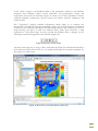
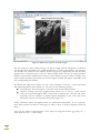
WiM-Med
USER MANUAL
V 1.1
Herrero, J., Aguilar, C., Millares, A., Egüen, M., Carpintero, M., Polo, M.J., Losada, M.
December 2010
Grupo de Dinámica de Flujos Ambientales
Centro Andaluz de Medio Ambiente (CEAMA) – University of Granada - Spain
Grupo de Dinámica Fluvial e Hidrología – University of Córdoba - Spain
2
Table of contents
Table of contents .............................................................................................................................. 3
List of figures ..................................................................................................................................... 4
List of tables....................................................................................................................................... 5
1.
Introduction .............................................................................................................................. 6
2.
System requirements and performance ................................................................................. 8
3.
Set-up.......................................................................................................................................... 9
4.
Data Organization: Wim-Med Project ................................................................................ 10
5.
Graphical environment .......................................................................................................... 11
6.
Running a case study .............................................................................................................. 12
Project........................................................................................................................................... 13
Project Properties ....................................................................................................................... 13
Project tree ................................................................................................................................... 19
Results .......................................................................................................................................... 30
Printing. Print preview. .............................................................................................................. 34
Appendix A. Organizing the information. .................................................................................. 35
Appendix B. Format of data files. ................................................................................................ 40
Raster-map files ........................................................................................................................... 40
Sequence Files ............................................................................................................................. 41
Aquifers file (h1) ......................................................................................................................... 42
Files of meteorological stations (m1) ....................................................................................... 43
Meteorological data files ............................................................................................................ 43
File of weather events (m2) ....................................................................................................... 44
Appendix C. Spatial structure of calculations ............................................................................. 46
General scheme ........................................................................................................................... 46
Cells with surface balance .......................................................................................................... 48
Cells with circulation on slopes ................................................................................................ 49
Cells which contribute to aquifers ............................................................................................ 50
Point flow results ........................................................................................................................ 50
Results distributed by cell .......................................................................................................... 51
3
List of figures
Figure 1: About... ............................................................................................................................. 7
Figure 2. Set-up. Start-up screen. .................................................................................................... 9
Figure 3. Set-up. Selection of components. .................................................................................. 9
Figure 4. Dynamic help label......................................................................................................... 11
Figure 5. Display properties. ......................................................................................................... 11
Figure 6. WiM-Med main window. .............................................................................................. 12
Figure 7. General and topographic properties. ........................................................................... 14
Figure 8. Detailed topographic properties. ................................................................................. 15
Figure 9. Meteorological properties. ............................................................................................ 15
Figure 10. Viewing an ASCII text file with the meteorological stations. .............................. 16
Figure 11. Soil properties. .............................................................................................................. 16
Figure 12. Advanced soil properties. ............................................................................................ 17
Figure 13. Vegetation and hydrological properties. ................................................................... 18
Figure 14. Advanced hydrological properties. ............................................................................ 18
Figure 15. River properties (floods). ............................................................................................ 19
Figure 16. Digital Elevations Model............................................................................................. 20
Figure 17. User map regions.......................................................................................................... 21
Figure 18. Aspects map. ................................................................................................................. 22
Figure 19. Map of horizon height in the direction of NW-SE................................................. 22
Figure 20. Sequence control toolbar. ........................................................................................... 23
4
List of tables
Table 1. Types of simulations allowed. ........................................................................................ 35
Table 2. List of data required, according to type of simulation. .............................................. 35
Table 3. Data from the tree in the main WiM-Med window.................................................... 36
Table 4. Data in the Project Properties window with codes. ................................................... 38
Table 5. List of active intermediate variables, according to simulation type. ......................... 38
Table 6. List of active state variables, according to simulation type. ...................................... 39
Table 7. List of active meteorological variables, according to simulation type...................... 39
5
1. Introduction
WiM-Med (Watershed Integrated Management in Mediterranean Environments) is a program that
allows us to simulate watersheds using a complete, distributed physical model. Working
from daily and hourly weather data, it facilitates the spatial interpolation and temporal
distribution of meteorological variables, the simulation of distributed hydrological
processes that occur both on and under the ground, calculating the water balance in
aquifers and the generation of groundwater flow, circulation on mountain slopes and river
channels and the non-permanent study of rivers during flood events. The following soil
processes are calculated in a distributed way: interception, snow, surface runoff,
evaporation, surface infiltration, subsurface flow and groundwater recharge. As the name
suggests, it has been developed with a view to becoming part of a technical tool which will
facilitate, and also provide a solid scientific basis for, integrated watershed management.
Thus, the WiM-Med model allows us to deal with every aspect connected with water and to
transfer a specific combination of meteorological variables acting on a particular region to
results which are both occasional and widely distributed in space, such as river water flow,
volume of stored water or the size of flooded areas.
The WiM-Med model, although it can be applied to any watershed, has been developed in
the basin of the River Guadalfeo, in the Andalusian Mediterranean Basin, and therefore
special attention has been paid to faithfully representing the processes linked to a semi-arid,
mountainous Mediterranean basin with snow, torrential rains, lengthy periods of drought, a
notable presence of groundwater and a marked heterogeneity in all its physical properties.
The program is made up of two separate parts: a calculation module and a Windows
viewer. The calculation module is an expert program, run by command line and interacting
with the user through entry and exit files. It is responsible for carrying out all the
calculations and hydrological simulations. The Windows viewer is a graphical environment
that allows for more user-friendly interaction in data selection and preparation and in
displaying results.
6
Figure 1: About...
The WiM-Med Cmd calculation module has been developed and tested jointly by the
Environmental Flow Dynamics Research Group of the University of Granada (Grupo de
Dinámica de Flujos Ambientales, http://www.dinamicaambiental.com) and the Fluvial
Dynamics and Hydrology Research Group of the University of Córdoba (Grupo de Dinámica
Fluvial e Hidrología, http://www.uco.es/investiga/grupos/dinamicafluvialhidrologia/DFH/)
and the University of Córdoba Hydrology and Agricultural Hydraulics Group. The
Windows graphical display used by Wim-Med has been developed with the cooperation of
Bermasoft.com. All of the above has been carried out as part of the Guadalfeo Project,
funded by the Institute of Water of the Andalusian Regional Government’s Ministry of the
Environment.
7
2. System requirements and performance
WiM-Med is designed to work under the Windows operating system (XP or later). The disk
space required for installing the basic program is minimal: 5 MB.
However, it is during the calculation with the simulation model when there is a greater
demand on system requirements. In this case, both disk space and RAM memory, as well
the as computing time required, depend largely on the number of pixels the study area is
divided into, the number of days the simulation lasts and the number of calculation
variables for which results are required. Therefore, it is practically impossible to fix any
previous system requirements.
To give an example, we can state the specific requirements used during the simulation of
the particular case included in the Guadalfeo Basin study. The study area in this case was
made up of 1.5 million cells. The computer used was an AMD Athlon 2400+. The free
RAM needed is 1.5 GB (2 GB total minimum, including Windows). The disk size required
depends on the combination of the number of maps requested, calculation length and time
scale in which the results are needed, given that each map in this basin takes up about 10
MB. Using these data, we can estimate that a calculation with hourly results, for example,
would occupy 1GB of disk space for each variable and for each 4-day simulation period.
The program automatically calculates the disk space needed in order to alert the user if
there is any danger of running out of free disk space.
As far as processing time for the complete Guadalfeo Basin study is concerned (storing one
variable per day), using the hardware described above, we estimate it took 10 hours of
calculation per year simulated.
8
3. Set-up
The WiM-Med program is very simple to install, and uses the executable set-up file
wimmed_1.0.0.26.exe. If you run this program, a set-up wizard (Figures 2 and Figure 3)
opens where you can select the installation directory and the components to install.
Figure 2. Set-up. Start-up screen.
The optional components include only the help file and the sample project, which is what
takes up most of the installation, as it includes all the necessary data for carrying out the
River Guadalfeo Basin simulation.
Figure 3. Set-up. Selection of components.
9
4. Data Organization: Wim-Med Project
All the information with the data and results from the simulation in one particular region is
collected together in what is called a project. All the files added to the project are copied
into a folder with the same name as the project inside the directory My
Documents→WiMMed Projects. In other words, each WiM-Med project will always work with
its own copy taken from the duplicate of the original files. In this copy, the map files are
always stored in WiM-Med binary format, in order to reduce their size and disk-access
time.
The program directly processes and displays the information it generates. Thus, in the same
way that new simulations associated with a project can be launched, folders of previous
simulation results can also be deleted from inside WiM-Med. The corresponding result files
will be automatically deleted from the computer, since they often occupy a large amount of
disk space. In any case, an expert user can access all information connected with WiM-Med
through Windows Explorer. In this way, all projects, with their data files and results, can be
edited (deleted, copied, etc.). Each folder contains all the information relating to a project
(data and results). This direct access is not recommended when using the program
normally, and is only recommended for carrying out back-up copies or for deleting a
project completely.
Uninstalling the product does not delete the projects created with WiM-Med, and these can
take up a lot of disk space and must be removed manually from the abovementioned
folder.
Loading a project and all its associated data (whether to open or edit it) should be carried
out from the disk, and probably consists of a large amount of information. It is, therefore,
quite normal that it takes a few seconds to load.
10
5. Graphical environment
The visualization of data and results share a number of features which belong to the WiMMed graphical environment, which has been specially designed to present and manage
distributed information in map form:




Geo-referenced maps.
Dynamic on-screen information using labels (Figure 4).
Zoom and distance-measuring tool.
Display layers with variable viewing options: color scale, scale limits, decimals, and so
on. (Figure 5).
 Printing and Print Preview
 Storage of each case study in project form, with all input data and the different
simulations which have been carried out.
 Simple installation with built-in example.
 Export, import and display maps in raster ASCII-ArcGIS format.
 Export of maps in most common graphic formats (jpg, bmp, tiff, etc.)
Figure 4. Dynamic help label
Figure 5. Display properties.
The main WiM-Med graphical interface is divided into 3 main sections, as shown in Figure
6:

(1) Project bar: this is a tree which groups and orders all the input and output
information. It contains folders
with information, maps
and sequences . The
sequence is a set of maps which shows the temporal evolution of a particular geo-
11
referenced property. Thus, it can be viewed as a video in which each of its images is
linked to a date.
 (2) Map: this area of the maps features geo-referenced display with information
distributed by colour code This code appears on the side of the window, with reference to
its units.
 (3) Results bar: this is the text window where the main results messages for the
simulations in the different modules are shown..
Figure 6. WiM-Med main window.
In addition, there is the usual Status bar at the bottom of the window, where useful
information is displayed, such as, for example, the UTM coordinates of the mouse position
on the map. Finally, there is also a Menu and a Toolbar at the top of the screen, where the
different functions of the program can be accessed simultaneously.
All the bars mentioned (that is, all the graphic elements except the Menu and Map) can be
enabled and disabled from the menu item View.
6. Running a case study
12
This chapter describes, in the style of a set-up wizard, how to load, handle and display data,
run a simulation and visualize and export results. In this way, we can run through the
program's functions while describing the data required for calculation.
Project
From the File→New File→New menu, you can access a tutorial where all the input data is
asked for in sequence in order to create a new project. There is no need to specify all the
project data for this tutorial mode (a Digital Elevations Model is OK), so that any data not
yet defined can be loaded or modified afterwards from the Project→Properties option. The
windows showing the project properties definition are the same both for a new project
tutorial and for editing an existing one. These are dealt with separately in the next section.
An earlier project which has been saved can be loaded from the File→Open File→Open
menu or from the “recent documents” area opened in the File menu.
Project Properties
Whether you start from the new project tutorial or from the properties menu of an active
project, the windows which allow you to enter all the data needed for the simulation are the
same.
These input data can appear in any of the following four formats: number, formatted
ASCII text file, raster map or map sequences. The numerical definition of the parameters is
displayed directly in the windows. The formatted text files must be edited previously
following the instructions indicated for each type of data. Raster map formats must
correspond to either of the following formats: ASCII-ArcGIS or binary WiM-Med.
The input data are grouped into the following categories: general, topography,
meteorology, soil, vegetation, hydrology and river. Table 4 shows in detail the hierarchy of
all the data. The property definition windows, in general terms, reproduce this hierarchy. In
some of these main chapters, the sub-category Advanced Properties is included, which, in
general, groups together the properties which correspond to calibration factors or those
which are optional.
The first window (Figure 7) contains general properties and topographic properties. These
include one basic item of data, namely the Digital Elevations Model DEM, in map format.
In all these project data entry windows, there is a yellow box at the bottom which shows
expert information about the variable which is active (that which is being edited). This
information includes a detailed description of the variable, its units, its format and, where
applicable, it suggests a default value.
Data with non-numerical format need a text file to be introduced. On the right, there is a
button with a triangle
which allows you to find the file on the hard disk (examine) or to
13
view the contents of the selected file, but does not allow editing (example in Figure 10).
Such editing should be carried out outside WiM-Med, using any ASCII text file editor.
Figure 7. General and topographic properties.
The topographic properties category includes some advanced features which are shown in
Figure 8. All the topographic data collected here can be calculated automatically by WiMMed using DEM, so it is not necessary to define them. For the first simulation which is
carried out without them, they will be automatically generated and stored in a results
subdirectory in the project directory. This may take up a large amount of computing time,
especially for the DEM correction for flat or depressed areas, and for constructing the
DFM Digital Flow Model. To avoid having to repeat these calculations in successive
simulations, you are recommended to include in the project maps created in the first
simulation the project include through the advanced topographic properties shown in
Figure 8. In addition, data generated by other external applications can also be incorporated
into the project, taking care that the limits and number of cells of these maps are perfectly
matched with those of the DEM.
In this type of table, you can browse for a file by using the button which appears on the
right when a property is selected.
14
Figure 8. Detailed topographic properties.
Figure 9 shows the window through which the meteorological data are defined. All
correspond to ASCII text files with the format specified in Appendix B. Figure 10 shows
how WiM-Med presents a previously loaded ASCII text file, without allowing editing.
Figure 9. Meteorological properties.
15
Figure 10. Viewing an ASCII text file with the meteorological stations.
Figure 11 shows the data input window with the basic soil properties, all referenced to
maps. In addition, the advanced soil properties (Figure 12) include some numerical
parameters for a range of soil calculations and calibration coefficients for the previous
maps.
Figure 11. Soil properties.
16
Figure 12. Advanced soil properties.
The next window (Figure 13) lists the vegetation and hydrology properties. Under
vegetation characteristics, there is a map with the maximum storage capacity of the canopy
fraction and the two input items of data for a project which are defined as map sequences:
the fraction of plant cover and the albedo. A sequence is defined through an ASCII text
file which refers to a series of maps with the paired date-map sequence - Appendix B gives
a detailed description of this format. The sequences are related to a particular temporal
variability of the property. In this case, the variability of the plant cover is detectable from
satellite image processing, together with its date. If a suitable series of images is not
available, a single date-map pair with any date and a relevant map can always be included in
the ASCII text file of the sequence, taken as a time constant.
17
Figure 13. Vegetation and hydrological properties.
Figure 14. Advanced hydrological properties.
Finally, there are two ASCII text files with the properties needed for the river simulation
with the one-dimensional non-permanent model (Figure 15).
18
Figure 15. River properties (floods).
Project tree
The display of geo-referenced data (maps, sequences, and weather stations) is controlled by
the project bar or tree. This appears on the left-hand side of the task window (Figure 6,
area 1), and it shows the layers with data and results arranged in thematic folders. The
management of the data within the tree, following the criteria outlined in the Project
Properties, is detailed in Table 3 (Appendices section). At the highest level, there are the
three main folders, which are Input data, Results and User maps. At the lowest levels are the
relevant maps or map sequences. All the names in brackets refer to a folder or sub-folder.
The input data are grouped into sub-folders under the main categories in which all data are
included: General, Topography, Meteorology, Soil, Vegetation and Hydrology.
The colouring order of the layers is top downwards. This means that the highest layers in
the tree (DEM) are coloured first, and the lowest last, covering the previous ones. In any
case, only the DEM layers, regions and weather stations can be permanently active. The
remaining layers can only be activated one at a time.
19
Figure 16. Digital Elevations Model.
In front of each map there is a selection box to enable or disable the display of that layer.
Only the two layers in the General level can be permanently activated. For the other layers,
activating one layer automatically disables the previously selected one. The layer display
makes them overlap each other following the descending order of the tree. Thus, the layer
with the digital elevation model DEM (Figure 16) is always at the bottom.
The DEM is the starting data for any project, since it is from this information that the
extent, coordinate and accuracy (cell size) of all other maps are defined – both as input
(which must coincide with it) and as output.
The other map included in the “General” category is that of User regions (Figure 17). This
map simply serves to define the calculation area within the rectangular extension of the
DEM and establish characteristic regions where added results can be included.
20
Figure 17. User map regions.
In “Topography” are included maps which bear a direct relation to the orography and the
hydraulic network, which are both calculable directly from the DEM. Two examples of the
maps included in this category are the map of aspect or direction of maximum slope
measured from the south in a clockwise direction (Figure 18) and the map of horizon
height in the NW-SE direction (Figure 19), which indicates the height in degrees which the
horizon is at, at a fixed point looking from there to the SE.
21
Figure 18. Aspects map.
Figure 19. Map of horizon height in the direction of NW-SE.
22
In the “Soils” category, the distributed data of the parameters related to soil hydraulic
properties that influence surface runoff, subsurface and groundwater, storage and
evaporation from itself are collected. Figure 21 shows one of these parameters: surface
saturated hydraulic conductivity, which controls the balance between infiltration and
surface runoff.
The “Vegetation” category includes information which helps us to measure the
interception of rainfall by vegetation and albedo (Figure 22). This information is displayed
as maps and two sequences: the albedo and the canopy fraction. The sequences are a set of
maps showing one piece of land over different dates. Each date constitutes a map
equivalent to a still video image. To move around the different dates or images, use the
following control which appears on the Toolbar (Figure 20):
Figure 20. Sequence control toolbar.
It works in the same way as using a video, with frame-by-frame fast-forward and rewind, in
both directions. With red controls, we can enable and disable the automatic playback for
the sequence in video form.
Figure 21. Map surface saturated hydraulic conductivity.
23
Figure 22. Map of the sequence of albedo images.
The last category is that of Meteorology. As well as a map with the Hargreaves coefficient
and another that determines the spatial distribution of hourly precipitation, this category
also includes the situation of the weather stations (Figure 23), despite the fact that this layer
appears last on the project tree so that it is always visible above the rest. To make activation
linked to the weather variable easier, there are sub-folders for each of these variables. Any
station which measures more than one meteorological variable will appear repeatedly in all
the corresponding sub-folders.
By clicking the right mouse button on any of the elements of the tree, a contextual menu
will appear (Figure 24) from which you can carry out the following actions:
Exporting data. Save the map as a raster file with ArcGis ASCII format.
Properties. Change the map’s graphical map allows you to choose a new colours
scale, the lowest and highest limits of this scale, a transparency value for null values
(optional) and the number of decimal places displayed on the scale and in the
information about each dynamic label point (Figure 25).
Unless otherwise stated, the display limits are calculated automatically. In one sequence,
these limits remain constant for all images, in order to allow a clearer comparison between
them.
You can also obtain a representation of the maps in image file format (jpg, bmp, tif ,...)
from the menu File → Export Image.
24
Figure 23. Weather stations.
Figure 24. Contextual menu in the tree maps.
25
Figure 25. Options for displaying a map of the project tree.
26
Simulation
To run a simulation case, you can either start from the Project→Simulation menu, or with the
following buttons on the toolbar:
The buttons, from left to right, represent the permitted types of simulation - which are
described in Table 1 – as follows:
Simulation of surface cycle
Full-cycle simulation using Muskingum for the river routing
1-D river simulation model
The surface cycle simulation is the simplest of all. It allows us to make calculations of the
hydrological balance in each cell of the area studied without dealing with the generation of
flow. In other words, calculating the estimated runoff and infiltrations for each cell, but
without these circulating towards the channel and without calculating the groundwater in
the aquifer. To carry out a simulation of this type, the element should be selected from the
Project→Surface Cycle Simulation menu.
The following figures show the options available from the surface cycle simulation window,
although these options are common to all types of simulation.
Figure 26. Surface cycle simulation. Variables.
The simulation results you need to save for study or to include in a report are selected from
the variables tab (Figure 26). The variables for obtainable results depend on the type of
simulation (see Tables 5, 6 and 7). Once you have chosen the variable you want to get
results from, you must select the simplest (and fastest) simulation available.
27
From this window (interval column), it is also possible to choose the time scale for which
you want the results: hourly, daily, by event, yearly or total (over the whole simulation
period). The calculation column allows you to choose from distributed results in map form,
or accumulated by region. The distributed results will be transformed into a map sequence,
one for each time step according to the time scale selected. The accumulated results by
region are based on the regions map defined by the user in the project properties (key g1,
Figure 17) and present the average results for each region. Therefore, the result is displayed
as a table in ASCII format where each column represents a region and each row a time
step. The first column shows the average for all the regions. This file can be found in the
results directory with a suffix after its name which refers to the variable it contains,
according to the keys which are shown in Tables 5, 6 and 7.
The activation of a results variable means a significant increase in computing time as well as
in the free disk space required if it is in map form (at a rate of 10 MB per map sequence).
Figure 27. Simulation window. Dates interval.
On the “Dates” tab in the simulation window (Figure 27), the starting and ending dates for
the simulation are chosen. To help with the choice, the dates can be defined directly by an
expert Windows control (Figure 28), or by using the dates of precipitation events (“Events
File” in “Project Properties” - key m2 in Table 4).
The last tab allows you to select the active regions during the simulation based on the map
of regions defined by the user (key g1, Figure 17). When you only need results from a
particular area, choosing this calculation area greatly reduces the execution time.
28
Figure 28. Simulation window. Date selection.
Figure 29. Simulation window. Active regions.
Once the variables, dates and regions have been selected, you can launch the simulation
with the Generate button. A progress bar indicates that the model is calculating, during
which process no action can be taken on the agenda, except to cancel the simulation if
needed (Figure 30). The results window (Figure 31) shows the most significant incidents
during the loading of data and the current date when the simulation is running. An
important feature of this window is if there is an error, it pinpoints the cause, thus allowing
for correction. The duration of the calculation depends on the number of cells to simulate,
the simulation interval, the number of variables requested and the characteristics of the
computer. In the example shown in this tutorial, the period may be as much as several
hours.
Figure 30. Simulation progress window.
29
Figure 31. Results window.
Results
Once the calculation has been successfully completed, the simulation results will appear in
the Results category in the project tree, in a sub-folder with the date and time of when the
simulation took place. Previous simulations carried out on the same project are not deleted.
Each result variable asked for in map form leads to a map sequence, one for each date on
which a result has been generated, according to the selected time interval of results. In this
way, using the toolbar controls, it can be viewed as a video (Figure 20).
Figure 32 shows the result for the amount of daily snow (equivalent in water, measured in
mm) for a simulation lasting 10 days. The screen shows one of the images of the calculated
sequence, which consists of 10 maps, as indicated in the project tree after the name of the
variable in parentheses. The map title includes the name of the variable and the date which
the currently displayed image corresponds to. Each map in the sequence can be exported
individually as a Arc-GIS raster file in text format or as an image file, or it can even be
printed directly from the tree itself (by right clicking the context menu) or from the File
menu.
30
Figure 32. Map of results. Water equivalent of snow.
Figure 33 shows another example from the same simulation - in this case, total daily runoff.
31
Figure 33. Map of results. Surface runoff.
The maps referring to state variables (such as the water equivalent of snow) represent the
instantaneous state on the date of the map, whereas maps of the intermediate variables
(such as runoff), and weather maps, represent in some cases the average and in others the
accumulated value of that variable from the date of the previous map to the present one.
In the title shown in the geo-referenced display area, appears the name of the variable
calculated and a date corresponding to each map in the generated sequence. This date
changes according to the element of the sequence represented at each time. If daily results
are generated, the simulation date will be shown. With timetables, both the date and time
are shown. In the latter case, the hour (HH):00 refers to the fact that this map shows the
accumulated, average or final results of the time interval (HH):00 (HH+1):00.
By right-clicking on a results item in the project tree you obtain a drop-down menu from
which you can access the general properties of the sequence. As well as the display
properties (Figure 25), a tab appears in the window with general information (referred to as
Properties) about the simulation with which the sequence was generated, namely the starting
and ending dates of the simulation, the time step chosen for the results and the type of
simulation (Figure 34).
32
Figure 34. Properties of a sequence of results.
Apart from the results visible directly from WiM-Med, a series of files generated by a
simulation is stored on the hard disk inside the project directory (following the path My
documents→ WiMMed Projects →Name of Project) which can be consulted and copied. These
results are:
Individual maps that make up each of the results sequences
Results tables accumulated by region (with the identifier AXR in the name)
Text files showing the mm of water supplied to the drainage points in the form of
surface (with the prefix QSup in the name), sub-surface (with the prefix QLat) and
underground (prefix Ac_QTot) flow.
River flow (prefixes: QRio and Daily-QRio). The first has a mixed hourly-daily time
scale, and the latter is a daily average (only for Full-cycle simulation with
Muskingum).
Maps with the final values for State Variables, that allow you to continue with the
simulation by updating the meteorological data (with the prefix Tot_ and
identification of the variable according to the suffix shown in Figure 26).
Maps of topographical data which are generated in the calculation, but not defined
by it (slope, aspect, horizons, SVF, MDR, MDF and Drainage Regions - RD).
33
Printing. Print preview.
One last post-processing tool of interest is the capability to print a report of the map
shown at any time in the general window, with print preview included (Figure 35). This
option is accessed from the menu File-> Print preview or more directly, File-> Print. The map
has a caption which includes the properties of the simulation that produced it.
Figure 35. Print Preview.
34
Appendix A. Organizing the information.
Depending on the simulation chosen, the data required for calculation varies. The
following tables show a compilation of all the information you need to define to perform a
simulation and the information you can get from it, always depending on the simulation
type, as seen in the key in Table 1.
Hydrological Model
"
"
1-D River model
Erosion model *
Surface Cycle
Complete cycle with River (Muskingum)
River routing with GuadalFORTRAN
-
S1
S2
S3
S4
* In development
Table 1. Types of simulations allowed.
Table 2 shows what data must be defined for each of the two types of hydrological
simulation. The data are referred to by a code, consisting of a letter-number combination
that corresponds to the variables shown in Table 4.
Entry variables:
s1-s2-s3-s5
s4
s6
s7
r1→r5
r6-r7
g1-g2
h1-h3
h2
t1
t2-t3
t4-t5
t6→t15-t18
t16-t17
t20→t28
t40-t41
t42-t43
m1→m13
v1→v8
d1-d2
d3
c1→c10-c13→c20
c11-c12
S1
*
S2
*
*
*
*
*
*
*
*
(*)
(*)
*
*
(*)
*
*
*
*
*
*
*
*
*
(*)
*
*
(*)
*
*
*
*
*
* Obligatory data
(*) Data which is useful, but if not available, can be
calculated (Calculations based on DEM)
Table 2. List of data required, according to type of simulation.
35
The following two tables show the data which appear in the project tree (Table 3) and in
the properties window (Table 4), and their order.
[Entry data]
[General]
- Digital Elevation Model
- Regions
[Topography]
- Slope
- Aspect
- Digital Flow Model
- Digital Rivers Model
- Visibility Factor SVF
- Horizon direction N-S
- Horizon direction NE-SW
- Horizon direction E-W
- Horizon direction SE-NW
- Horizon direction S-N
- Horizon direction SW-NE
- Horizon direction W-E
- Horizon direction NW-SE
[Meteorology]
- Hargreaves’ Coefficient
- Spatial distribution of hourly P
[Soil]
- Saturated Surface Conductivity
- Saturated conductivity in soil
- Capacity of the sub-surface flow contribution
- Moisture saturation
- Residual moisture
- Matric potential of wetting soil
- Matric potential of drying soil
- Soil thickness (upper layer 1)
- Soil thickness (lower layer 2)
- Van Genuchten’s n parameter
[Plants]
- Storage capacity of vegetation canopy
- Albedo (*)
- Canopy fraction (*)
[Hydrology]
- Aquifers
- Speed of surface runoff
- Speed of sub-surface runoff
[Erosion]
[Results]
[User’s maps]
[Weather
Stations]
- [Daily precipitation]
- [Hourly precipitation]
- [Temperature]
- [Radiation]
- [Wind speed]
- [Vapour pressure]
- [Atmospheric
emissivity]
(*) Sequence
Table 3. Data from the tree in the main WiM-Med window.
36
+General
- Digital Elevation Model (t1)
- Regions (g1)
- Latitude (t16)
- Longitude (t17)
+Topography
- Threshold area for channel calculation [km ²] (d1)
- Correction factor for plains (d2)
- Height above sea level [m] (d3)
+ Advanced:
- Slope (t2)
- Aspect (t3)
- Digital Flow Model DFM (t4)
- Digital River Model DRM (t5)
- Visibility factor SVF (t20)
- Horizon direction N-S (t21)
- Horizon direction NE-SW (t22)
- Horizon direction E-W (t23)
- Horizon direction SE-NW (t24)
- Horizon direction S-N (t25)
- Horizon direction SW-NE (t26)
- Horizon direction W-E (t27)
- Horizon direction NW-SE (t28)
+Meteorology
- Weather Stations (m1)
- Events (m2)
- Hourly precipitation [-] (m3)
- Daily precipitation [mm] (m4)
- Daily Temperature [ºC] (m5)
- Daily solar radiation [MJ] (M6)
- Spatial distribution of the hourly P (m7)
- Hargreaves’ coefficient (m9)
- Daily wind speed [m / s] (m10)
- Daily vapour pressure [kPa] (m11)
- Daily long-wave emissivity [MJ / MJ] (m12)
- Starting dates of rainy season (m13)
+Soil
- Saturated surface conductivity (t6
- Saturated soil conductivity (T7)
- Capacity of sub-surface flow contribution (t8)
- Saturation moisture (t9)
- Residual moisture (t10)
- Matric potential of wetting soil (t11)
- Matric potential of drying soil (t12)
- Van Genuchten’s n parameter (T18)
- Soil thickness (upper layer 1) (t40)
- Soil thickness (lower layer 2) (T41)
- Speed of surface runoff (t42)
- Speed of sub-surface runoff (T43)
+ Advanced (Soil calculation parameters):
- Time for redistribution of water in soil [h] (c5)
- Exponent “alpha” to express evaporation (c16)
- Coefficient “beta” to express evaporation (c17)
+ Advanced (Calibration coefficients for maps):
- Saturated conductivity on surface (67)
37
- Saturated conductivity in soil (c7)
- Capacity of sub-surface flow contribution (c8)
- Saturation moisture (c14)
- Residual moisture (c15)
- Matricial potential of moist soil (c10)
- Matricial potential of dry soil (c9)
- Van Genuchten’s n parameter (c13)
- Soil thickness (upper layer 1) (c18)
- Soil thickness (lower layer 2) (c19)
- Speed of surface runoff (c11)
- Speed of sub-surface runoff (c12)
+Vegetation
- Storage capacity of vegetation canopy (t13)
- Canopy fraction (t14)
- Albedo (t15)
+Hydrology
- Data from aquifers (h1)
- Aquifer areas (h3)
- Definition of river (h2)
+ Advanced (snow):
- Diffusivity coefficient of recordable heat with no wind (c1)
- Snow roughness [m] (c2)
- Snow recession curve. EA *_100 parameter (c3)
- Snow recession curve. SCmin parameter (c4)
- Temperature with snowfall [ºC] (c20)
+Erosion
* (blue: constant, red: text file, black: map, green: sequence)
Table 4. Data in the Project Properties window with codes.
Finally, here are the types of results that can be obtained in each type of simulation, for
intermediate variables (Table 5), state variables (Table 6) and meteorological variables
(Table 7).
Intermediate Variables
Soil evaporation
Deep infiltration
Infiltration
Runoff
Snow evaporation
Snowmelt
Canopy evaporation
Interception
Frozen Rainfall
Sub-surface flow
Sediment deposition
Inter-furrow erosion
Furrow erosion
Unit Suffix
mm
EvS
mm
Per
mm
Inf
mm
Esc
mm
EvN
mm
Fus
mm
EvC
mm
Int
mm
Pcg
mm
Qlat
Kg/m² Dep
Kg/m²
Eri
Kg/m² Err
S1
*
*
*
*
*
*
*
*
*
*
S2
*
*
*
*
*
*
*
*
*
*
S4
*
*
*
*
*
*
*
*
*
*
*
*
*
Table 5. List of active intermediate variables, according to simulation type.
38
State Variables
Canopy humidity
Snow Water equivalent
Soil moisture Upper Layer1
Soil moisture Lower Layer2
Internal energy of snow
Snow density
EAMax of snow cycle
Surface Moisture
Surface Flow mm
Active sediment in cell
Solid flow in cell
Unit
mm
mm
mm
mm
MJ
kg/l
mm
mm
mm/h
Kg/m²
Kg/m²·h
Suffix
HCub
EAn
HSol1
HSol2
U_n
d_n
EAmx
HSup
QSup
PSol
QSol
S1
*
*
*
*
*
*
*
S2
*
*
*
*
*
*
*
S4
*
*
*
*
*
*
*
*
*
*
*
Table 6. List of active state variables, according to simulation type.
Meteorological Variables
Unit Suffix
Long-wave emissivity of MJ/MJ Eat
atmosphere
Vapour pressure
kPa
e_m
Wind speed
m/s
V_m
ET0
mm
ET0
Solar radiation
MJ
R
Direct solar radiation
MJ
Rdr
Diffuse solar radiation
MJ
Rdf
Temperature
ºC
T_m
Precipitation
mm
Pre
Snowfall
mm
P_n
S1
*
S2
*
S4
*
*
*
*
*
*
*
*
*
*
*
*
*
*
*
*
*
*
*
*
*
*
*
*
*
*
*
*
Table 7. List of active meteorological variables, according to simulation type.
39
Appendix B. Format of data files.
Raster-map files
Raster-map files are all those that contain spatial morphological information related to
matrix cells of the basin, with a value per cell. All these files should be standard import and
export grid or ASCII raster, with data separated by blank spaces, like those used by ArcGIS,
so they are readable and can be edited from a standard GIS environment. These files have
a heading with metadata in the following format:
ncols
nrows
xllcorner
yllcorner
cellsize
NODATA_value
nº-of-columns
nº-of-rows
coordinate-x-bottom-left-edge
coordinate-y-bottom-left-edge
size-of-cell-in-m
value-not-considered-as-data
After this, the data is included, separated by blank spaces in columns and free lines in the
rows. ncols and nrows are the number of rows (Y coordinate) and columns (X coordinate) of
the raster. xllcorner and yllcorner refer to the coordinates of bottom left-hand point of the
raster, cellsize to the size of the grid, which must be square, and the NODATA_value to the
value not considered as data. -9999 is a typical value for this code.
You can also enter the files in WiM-Med binary format, which is just a binary version of
the ASCII-ArcGis files. The fact that they are binary allows them to be read and recorded
onto disk much faster. In this case, the heading is converted into a sequence of 2 x 2-byte
integers (C/C++ short type) and 4 x 4-byte decimal (C/C++ float type). Next will follow all
the data in float format.
Muskingum river network configuration - Drainage points (h2)
This file is used to define significant points in the river network and the properties of the
channel sections all together for use in a type S2 simulation (complete simulation with
channel flow). WiM-Med deals with complex river networks, formed by any number of
branches as the user wants to define. The file is written out with a line for each new item in
the channel which you want to define. You can also introduce comment lines preceding
them with % symbol. There are two types of items: nodes (joints and junctions) and
reaches. The reaches must be defined between existing nodes. The river delineation module
automatically join the starting and ending node of each reach and add to it every node over
passed during its path. Only the nodes used by an active reach will be part of the river
network.
Every node is defined, one per line, with the following information:
An N character for node.
40
Exclusive Id Identifier, from 1 onwards. This identifier is, for example, the one
which will later be used in defining the properties of aquifers (h1) or will be show
in flow results files.
UTM coordinates. If any point is not situated in the river channel, as calculated by
DFM, it is automatically moved there according to the direction of flow. Repeated
points or those situated outside the drainage network will be automatically deleted.
Gauged or ungauged point (1/0). Every node included in the river network will be
treated as a subbasin generator, but only the outflow for the nodes marked as
gauged will be stored in the results files.
Optional description of any length, blank spaces allowed.
Reaches are defined as follows:
An R character for reach.
Id identifier of the initial node
Id identifier of the final node
Mean value for Manning roughness in the reach
Mean width of the reach
Optional description of any length, blank spaces allowed.
The nodes defined in this file are the reference to be used for files of specific results of
surface, subsurface and underground flow for the simulation with the 1-D River Model for
avenues. The river network defined with the reaches must be coherent. This means that
several reaches can share ending joints, but every joint can only be used once as starting
point for a reach. One reach can take as ending point an intermediate node belonging to a
second reach. In this case, the user must check that the automatic delineation is able to find
it in its path from the starting to the ending point of the second reach, or the first reach
will remain disconnected from the river network.
In this example, there are two reaches. Main reach (Guadalfeo River) runs from node 1 to
node 4. Automatic delineation of this reach crosses over node 3 and consequently split this
main reach in two parts. A tributary, Trevélez River, runs from node 2 to node 3. Thus,
node 3 works as a junction in this little river network. Only the outflow in node 4 will be
stored in the results files:
% Nodes (N id X Y Gauge-OutFlow(1/0) Description):
N1
482714 4095537
0
Guadalfeo headwater
N2
478451 4102319
0
Trevélez.headwater
N3
467295 4084157
0
Guadalfeo and Trevélez junction
N4
466943 4083675
1
Dique del Granadino
% Reaches (R InitialNode FinalNode Active(1/0) Manning MeanWidth(m) Description)
R1
4
1
0.035 4
Guadalfeo river to Dique del Granadino
R2
3
1
0.035 3
Trevélez river
Sequence Files
The files for ground cover fraction (t14) and albedo (t15) are map sequence files, which
show the available maps for this variable, with date. Each row contains a date and a map. It
is not important for the rows to be shown in any given order, either alphabetical or by date.
During implementation of the program, the daily map is interpolated from earlier and later
versions available at the current date.
41
The date format will be year/month/day, separated by blank spaces. The file path can
include directory modifiers (\), but be careful that the file path is the correct one from the
location of this file.
Example:
2002 11 25 .\datos\cubiertavegetal\20021125_fv.bin
2003 01 28 .\datos\cubiertavegetal\20030128_fv.bin
Aquifers file (h1)
The definition of all the parameters necessary for the calculation of the aquifers takes place
through a single file (h1) in text format. This file has a heading with three comment lines,
followed by as many lines as you need to define all the aquifers. Each line includes all the
properties of each of these aquifer regions in the following sequence:
An integer (greater than 0) is used as the ID for the aquifer, which coincides with
the ID included in the aquifers map (h3). It is extremely important that the indices
for the map and for this configuration file correspond. Indices appearing in this file
(h1) which are not included on the map are ignored. Indices found in the map (h3)
and not in (h1) will not be resolved, which means they will become non-aquifer
cells. IDs do not need to be consecutive.
1 / 0 indicates that the aquifer is active / not active for this simulation (which
allows you to disable parts of the model without having to make new maps.)
ID of the drainage point for the aquifer area, according to the key established in the
river file (h2). It is valid to use any type of river file point.
Storage coefficient kVZ for soil transition deposit to the aquifer area, in units of days
– decimals can be used.
Storage coefficient kDRRcauce for the rapid response deposit for the outlet to the
channel, in units of days – decimals can be used.
Storage coefficient kDRRperc for the rapid response deposit for the outlet to the slow
response deposit, in units of days – decimals can be used.
Threshold h0DRR for rapid response deposit for carbonated or detrital material, in
mm of soil – decimals can be used.
Specific performance corresponding to the rapid response deposit material SyDRR ,
expressed as a decimal fraction.
Storage coefficient kDRL for the slow response deposit for the outlet to the channel,
in units of days – decimals can be used.
Threshold for the slow response deposit h0DRL, in mm of soil – decimals can be
used.
Specific performance corresponding to the slow response deposit material SyDRL,
expressed as a decimal fraction.
Level at the start of the simulation for the rapid response deposit mm0DRR in mm of
water and using decimals.
Level at the start of the simulation for the slow response deposit mm0DRR in mm
and using decimals.
42
Area which contributes to evaporation from aquifer Aevap due to the proximity of
the water table to the surface, expressed in decimals.
Minimum threshold of water in the aquifer hET0 for it to produce maximum
evaporation (equal to ET0), in mm of soil.
Threshold of the slow response reservoir hminEv , below which there is no
evaporation, in mm of soil.
Free description of the aquifer, with blank spaces, up to the end of the line.
Example:
Aquifers in the Vadose area, + aquifer as two deposits in line
Guadalfeo River Basin
Id Act IdP kVZ kRc kRp h0R SyR kL h0L SyL mmVZ mmR mmL Aev hET0 hminEv Description
1 0 1 5 10 3 0 0.99 17 0 0.99 0 0 0 0.01 5 1 Cádiar aquifer area
3 0 6 10 10 5 0 0.99 25 5 0.99 0 0 0 0.05 5 1 Contraviesa aquifer area
Files of meteorological stations (m1)
This file is useful to determine the location and height of all the meteorological stations
which may be used in any of the meteorological data files. Each station is defined through a
series of data: identifying code, X-coordinate, Y-coordinate, height and name. Even if the
station itself is the source of more than one weather record, it is not necessary to include it
more than once in this file. In the heading of the meteorological files which require station
identification (m3-m6 and m10-m12) it will be referred to with the identifier assigned to
this file, which is an integer greater than 0. The station name is given solely for information
purposes, and is formed by a line of characters. Coordinates X, Y and Z may include
decimals.
Therefore, in the meteorological stations file there will be a line for each station. In each
line, the following information, separated by spaces, will appear:
Station No.
X-Coordinate
Y-Coordinate
Z-Coordinate
Station name
Example:
2 481882 4071816 246 ALBUÑOL
3 443816 4087267 734 ALBUÑUELAS
6 438464 4065578 30 ALMUÑECAR
27 486254 4092793 1208 MECINA BOMBARON
Meteorological data files
The different files with the meteorological variables to be used (measured or calculated
outside WiM-Med) open at the beginning of the simulation and the data can be accessed
43
when it is needed. Each row of the file contains the data at all the stations for a given day.
The first row indicates the day the data started and after that, the values of all the
consecutive days are given, with a new row for each day of data. To avoid unnecessary
calculation time, the data is not stored except for the cumulative variables that are
considered appropriate. The meteorological data includes daily and hourly rainfall, typical
daily temperatures (maximum, minimum and mean), daily accumulated radiation, daily
mean vapor pressure, average daily atmospheric emissivity and average daily wind speed.
The format of all these files will be similar for any meteorological variable; in no cases are
incomplete series allowed and all values will be taken literally as valid (including -9999).
February 29th in leap years will always be included.
The file configuration is, then, as follows:
a first row with the starting date of data in the dd mm yyyy format.
a second row with the index for the stations corresponding to each of the
subsequent measurements, in the same order as the subsequent data. This index
should be the same as that which appears in the file of meteorological stations
(M1).
next, in sequence, one row for each day of data. In the daily files, there is usually
one item of data each day in each season. But in the temperature files, there are
three items of data per station and day, ordered as maximum temperature,
minimum temperature, and then mean temperature. Also, the hourly files, each
station will have 24 items of data, one for each hour.
Example of daily temperature file:
25 1 2001
32 92 93
14 4 9 13.8 9.4 11.6 8 0.2 4.1
22 10 16 17 10.6 13.8 11.4 4.2 7.8
14 5 9.5 15.6 4 9.8 9.4 -1.2 4.1
Example of daily rainfall file:
1 9 1968
236
000
000
000
1.2 3.5 5.0
0 1.0 2.2
000
000
File of weather events (m2)
The proposed physical model considers the event as the main meteorological driving-force
in the Guadalfeo river basin. Events, associated with storms that leave rainfall over the
basin, last for a series of consecutive days, during which the processes dealt with by the
model are different from those simulated during the periods between events. Eventsstorms are numbered and catalogued. The index of the event corresponding to each day
44
after a given date will be entered in this file, with a 0 for those days when there is no event
in the watershed. Generating this database of events is important, because on those days
when the event is classified as 0, the model will not take rainfall into account, even if there
is data indicating daily or hourly precipitation.
The format is exactly the same as that of meteorological data, except for the second row of
stations, which is omitted, since the event is general and is not linked to specific points.
The first valid item of data begins after the date line.
Example:
1 9 1968
0
0
0
1
1
0
0
0
2
2
2
2
0
45
Appendix C. Spatial structure of calculations
The simulation of the hydrological cycle with WiM-Med involves a variety of elements on
different spatial scales which interact with each other in different ways. To analyze the
results correctly, and efficiently manage entry data, it is necessary to understand these
relationships, which are sometimes complex – therefore, they are illustrated visually in this
chapter, so as to facilitate understanding.
General scheme
The simulated cycle starts with the distributed calculation of rain and other meteorological
variables necessary in each active cell in the domain of study. The mass and energy balance
in each of the deposits associated with each cell allows us to obtain, for every state,
interception values, evaporation from the ground cover, evaporation from the snow,
snowmelt, surface runoff, infiltration, soil evaporation and seepage into the aquifer, along
with mass and energy levels of deposits. Surface runoff is transported via a circulation
model from each cell of origin to previously-selected drainage points. Simultaneously, the
ground water is added in deposits related to the aquifer that also trigger flow at specific
points, according to their levels. This, in simplified form, is the mechanism used to make
the change from the distributed scale of the terrain and rainfall to the spatially discrete scale
of the channel.
46
Figure 36. General scheme of the spatial relationship between elements of WiM-Med.
Figure 36 shows the general scheme of the data which influences the spatial extent of the
calculation and the transfer of distributed results to other discrete items – usually, flow. In
this set of scales and domains, the users’ regions, aquifer areas, sub-basins automatically
extracted from the digital flow model and the aquifer drainage points are all mixed
together. Later, we will look in more detail at each part of this scheme.
47
Cells with surface balance
Figure 37. Scheme of cell determination with active surface balance.
Not all the DEM cells are active. Calculations will only be made for those specifically
indicated. These will be defined by the intersection of the cells in the areas which are
activated for the simulation with the aquifer cells which are activated (in h1).
The so-called user areas refer to arbitrary extensions which may have some physical,
hydrological or practical meaning for the user, and which may provide results of any
variable accumulated by each region at different time scales.
Aquifer areas, on the other hand, are defined by the user. An aquifer area may contain cells
from outside the surface sub-basin beneath which it lies, or even outside the main basin, if
the characteristics of groundwater flow are such. Also, cells within the basin may not be
considered as inside any aquifer area of that basin, which is the same as saying that the
infiltrated water in them flows out of the basin.
This working scheme lends the program enough flexibility to be able to simulate complete
watersheds or only parts of them; the whole aquifer system or only particular aquifers. All
this is possible without having to change the maps that define the regions – all that needs
to be changed are the lists that mark active areas for the present simulation.
For all the cells with an active surface balance, the interpolation and distribution of
meteorological variables will be carried out, and all calculations of mass and energy balance
that are relevant to the type of simulation chosen will be performed.
48
Cells with circulation on slopes
The surface drainage system will be automatically calculated by the model through the
DFM (t4) digital flow model (which, in turn, is read or calculated from the DEM) and from
the list of surface drainage points defined in the river (h2). With a consistent DFM, the
program will calculate the sub-basins which belong to each of the points read. However, it
is the user’s responsibility to compare the consistency or agreement of the results obtained
with expected results. To facilitate this, WiM-Med will save, whenever you need to calculate
it, the DRM digital rivers model and the map of drainage regions or DR sub-basins which
are deduced from the data in the results directory.
Figure 38. Scheme for determining the active surface drainage network.
To calculate these sub-basins (the DR map), a particular draining point to any cell which is
not active on the surface can even be included as a contributing area. In this case, the cell
in question will not contribute to flow at that point since the surface balance has no effect
on it. This is what happens in the detail in Figure 38, where parts of the four sub-basins
that extend towards the south are in non-active cells and they are therefore not
contributing to runoff. If any of the sub-basins for one of the drainage points does not
contain any active cells, it will appear in the result file of surface flows but with a result of
zero for all the time states.
The common practice will obviously be to use user regions which match with existing
major sub-basins in the study area, but in this case, we must not forget that the real subbasins for the model will always be those deduced from the DFM and the drainage points,
and that the only utility of the user’s regions will be to define active cells and to define
accumulation areas and average results.
49
Cells which contribute to aquifers
Figure 39. Scheme for determining the active underground drainage system and its contributing
cells.
Each region has an associated active drainage point (h2), where, supposedly, all its water
flow pours. This point does not necessarily have to be in the area, but it does have to be on
the network of channels as defined in h2. The series of points, one for each active aquifer,
determines the underground drainage network.
Point flow results
The reasons for changing from the distributed to the point scale are based on the drainage
networks. The balance of mass in the underground reservoirs will result in a flow for each
aquifer area, which, due to the underground drainage system, allows an average level of
water to pass in an extension to a sporadic flow which is distributed in time. In turn, the
circulation of surface runoff through the DFM will concentrate the water at specific closing
points of the sub-basins with their corresponding phase interval.
Figure 40. Scheme for the generation of sporadic flow from drainage networks.
50
Results distributed by cell
Figure 41. Scheme for the generation of distributed results using active cells.
Furthermore, the distributed results which you want to save will be saved in map form
showing results in all the active cells, irrespective of whether they are in the user’s region or
the aquifer area. The accumulated results by region will be shown, obviously, only in those
regions defined by the user and activated by them, and therefore, there does not need to be
a correspondence between both sets of results (distributed and accumulated).
51