Download an extended semantic definition of pascal

Stanford Program Verification Group
Report No. 18
. June 1980
Department of Computer Science
Report No. STAN-CS-80-E) 11
AN EXTENDED SEMANTIC DEFINITION OF PASCAL FOR PROVING
THE ABSENCE OF COMMON RUNTIME ERRORS
bY
Steven M. German
Research sponsored by
Advanced Research Projects Agency
and
Rome Air Development Center
COMPUTER SCIENCE DEPARTMENT
Stanford University
An Extended Semantic Definition of Pascal
for Proving the Absence of Common Runtime Errors
by Steven M. German
We present an axiomatic definition of Pascal which is the logical basis of the Runcheck
system, a working verifier for proving the absence of runtime errors such as arithmetic
overflow, array subscripting out range, and accessing an uninitialized variable. Such
errors cannot be detected at compile time by most compilers. Because the occurrence
of a runtime error may depend on the values of data supplied to a program, techniques
for assuring the absence of errors must be based on program specifications. Runcheck
accepts Pascal programs documented with assertions, and proves that the
specifications are consistent with the program and that no runtime errors can occur. Our
axiomatic definition is similar to tloare’s axiom system, but it takes into account certain
restrictions that have not been considered in previous definitions. For instance, our
definition accurately models uninitialized variables, and requires a variable to have a
well defined value before it can be accessed. The logical problems of introducing the
concept of uninitialized variables are discussed. Our definition of expression evaluation
deals more fully with function calls than previous axiomatic definitions.
Some generalizations of our semantics are presented, including a new method for
verifying programs with procedure and function parameters. Our semantics can be easily
adopted to similar languages, such as ADA.
One of the main potential problems for the user of a verifier is the need to write
detailed, repetitious assertions. We develop some simple logical properties of our
definition which are exploited by Runcheck to reduce the need for such detailed
assertions.
This research was supported by the Defense Advanced Research Projects Agency under contract
MDA903-80-C-0159 and by the Rome Air Development Center under contract F30602-80-G
0022.
_----
Llhtroduction
In most programming languages, there are various undefined conditions and illegal
operations such as arithmetic overflow and array subscripting out of range. We call
t h e s e c o n d i t i o n s runtime errors b e c a u s e they are violations of language or
implementation imposed restrictions on program execution. Current compilers do not
attempt to detect runtime errors during compilation, though they commonly insert
special code to test for certain errors during execution. This approach is costly in
execution time and compiled program size, and of course gives no assurance that a
program will run to completion.
The occurrence of a runtime error may depend on the values of data supplied to a
program. For this reason, any technique for assuring the absence of runtime errors must
be based on some method for specifying programs.
Showing the absence of runtime
errors is thus a natural problem in program verification.
We have been developing an automatic verifier for proving the absence of runtime
errors in the language Pascal.
The Runcheck system takes as input a Pascal program
with entry, exit and optional invariant assertions, and proves that the specifications are
consistent with the program and that no runtime errors can occur. Invariant assertions
are not required in many cases because the system is able to generate simple invariants
automatically, but more subtle invariants must be supplied by the user. The system
currently checks for the following kinds of errors: accessing a variable that has not been
assigned a value, array subscripting out of range, subrange type error, dereferencing a
NIL pointer, arithmetic overflow, division by zero, control stack overflow, exceeding
heap storage bounds, and UNION’ type selection errors. The verifier and our semantic
definition of Pascal do not yet include REAL or SET types, but pointers are permitted.
Obviously, the notion of runtime error does not include every kind of programming
’ The language accepted by the verifier includes verifiable UNION types instead of Pascal’s variant records. Refer to [3] for
discussion of the problems of variants and the details of our UNION types.
a
2
error.
Introduction
The runtime errors for a langauge are the conditions under which progams
cannot continue to execute or continued execution would give undetermined results. For
a program to be useful, one needs to know more about it than that it does not have
runtime errors. Consider a program which is intended to copy a list made of pointers
and records; it can have an error which causes it to produce the wrong result without
any runtime errors in the sense we are using. Runcheck makes it possible to verify such
a program at several levels of detail. For the least detailed verification, the program is
submitted to Runcheck without additional specifications related to list copying. In this
case., Runcheck attempts to prove only that the program is free from runtime errors. In
general, it may be. necessary for the user to supply some specifications and invariants
even at this level of detail. For instance, the program may have a control stack
overflow unless the input is acyclic. User supplied invariants would be needed in case
the simple invariants generated automatically by the system are not sufficient to prove
absence of runtime errors. A more detailed verification could be obtained by adding
specifications saying that the result of the program is a copy of the input. An even
more detailed verification could establish bounds on the performance of the program,
such as the maximum number of times each statement is executed as a function of the
input [ 101.
The purpose of Runcheck is to automate the routine aspects of the least detailed
verifications, while still allowing the user to supply additional information for more
detailed verifications. Thus although Runcheck is primarily used to perform shallow
verifications, it provides a general logical framework for proving detailed properties.
Every program verified by Runcheck is assured to have, as a minimum, the property
that no runtime errors can occur if the entry assertion is satisfied.
This paper is concerned with an extended axiomatic definition of Pascal, which is the
logical basis of Runcheck.
The extended definition is similar to the familiar Hoare
axiom system IS], but it takes into account certain restrictions on the computation that
have not been considered in previous axiomatic language definitions.
Introduction
.
3
Although the details of our semantic definition refer specifically to Pascal, most of the
ideas are broadly applicable. The runtime errors which exist in Pascal are also present
in many other languages, and the ideas in our semantic definition can be adopted to
other languages with additional kinds of errors.
ADA 171 is an especially interesting
case; it should be possible to define much of the language by generalizing our definition
of Pascal. For instance, the problem of generalizing our definition to allow dynamic
subrange types is discussed briefly in section 8.1.
Our axiomatic definition of Pascal consists of some first
order theories plus axioms and
.
inference rules for reasoning about programs. One of the first order theories concerns a
predicate, DEF(x), which is true of expressions having a well defined value. The other
first order theories are familiar ones such as arithmetic. Runcheck is more than a direct
implementation of these logical components; a practical program verifier should provide
as much assistance as possible, e.g., in generating inductive assertions.
All of t h e
example programs discussed in this paper have been handled completely automatically
by the system.
Practical results with Runcheck have been reported in 121. An earlier approach t o
formalizing the extended semantics is presented in collaboratjon with D. Luckham and
D. Oppen in [4].
The theorems in the Hoare axiom system are of the form, P{A)Q Intuitively, this
formula states that if P holds before executing a program A, then if and when A
terminates, Q will hold. In [5,6] and elsewhere, the relation P{A)Q is taken to be true
if there is a runtime error in executing A. Hoare chose to make the interpretation that
if an error occurred, the effect of the program would be “undefined,” as if the program
had failed to terminate.
In our extended semantics, mAj’@, is defined to mean that if P holds, then A executes
without runtime errors, and if A terminates Q will hold. Since virtually all programs
are intended to execute without runtime errors, a proof of PEAI]Q is much more useful
Introduction
4
than one of P{A)Q, from a practical point of view. 2 If it is possible to verify the absence
of runtime errors in a program, the implementation can omit the usual runtime error
checking code -- an increase of efficiency without loss of reliability. Also, the extended
semantics is a convenient system for showing the absence of certain errors in programs
that are not intended to terminate.
Our proof system is general purpose in that any partial correctness specification can be
expressed by choosing P and Q Absence of runtime errors is proven together with
other properties.
There are other possible formulations; one could develop a proof
system based on statements of the form SAFELP, A], meaning that if P holds
beforehand, then A executes without runtime error. The disadvantage of such a system
is that proofs of the absence of runtime errors often require lemmas about more general
properties of the program.
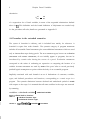
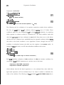
For example, consider a simple program which searches in an array A for an element
equal to KEY. The elements are stored in AD], . . . ,A[N-I]. The fast linear search
stores the key in the last position of the array A before searching, so that the search
,loop does not have to test whether the index has become greater than N. The result of
the search is returned in the variable I.
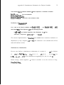
Example 1: Fast Linear Table Search.
VAR N:INTEGER;
TYPE ARR=ARf?AY[l :N] OF INTEGER;
PROCEDURE SEARCH(KEY:INTEGER; A:ARR; VAR I:INTEGER);
GLOBAL (N);
ENTRY DEF(N) A l<N A NMAXINT;
BEGIN
A[N]:=KEY;
I:=1 ;
WHILE A[I&KEY DO I:=I+l ;
END;
2 Thewe are cases where the difficulty of proving absence o f rll runtima errors outweighs the4 additional benefit.
approach in such cases is to leave some errors unchecked
A practical
Introduction
5
This program depends on the fact that A[N] has the value KEY throughout execution
of the loop. Otherwise, if the key was not found in A, the loop would continue and
attempt to access A[N+l], causing a subscripting error. It is necessary to prove that
A[N]=KEY is an invariant of the loop, and in our extended semantics, such lemmas can
be proven together in one step with the proof of absence of runtime errors
The procedure SEARCH is presented to the Runcheck system with an ENTRY assertion
stating that N has a value between 1 and MAXINT, the largest integer. The system is
able in this case to verify absence of subscripting errors, arithmetic overflow, and
uninitialized variable errors (the use of the value of a variable before it has been
assigned a value), automatically, given only the ENTRY assertion and program text as
shown in Example 1. In particular, the necessary loop invariants including A[N]=KEY
are generated automatically without any effort on the part of the user. The reader is
warned not to form an opinion of the system’s capabilities on the basis of this small
introductory example alone; a variety of more interesting programs have been handled
by the system. Some of them can be found in section 7 of this paper and in [Z].
This paper is divided into nine sections and two appendices. Section 2 contains
important definitions, particularly the definitions of the language and notation of the
extended semantics.
Section 3 is mainly concerned with the predicate DEF, which is
true of expressions having a well defined value. Section 4 presents some of the basic
inference rules of the extended semantics.
Section 5 presents a precise axiomatic
definition of the evaluation of expressions in Pascal. In section 6, the definition of
expression evaluation is used as the basis of a definition of Pascal statements, functions,
and procedures.
are
valuable
Section 7 develops some properties of the extended definition that
when
verifying
actual programs.
Section 8 discusses some
generalizations of the extended definition, including a new method of verifying
programs with procedure parameters.
Following this is a discussion of our general
conclusions. Finally, Appendix A gives details of the implementation of the extended
semantics in Runcheck, based on the principles developed in section 7, and Appendix
Introduction
6
B discusses the details of a definition of simultaneous substitution for disjoint Pascal
variables.
2. Preliminaries
2.1 General definitions
reference class (see Cl l]), used to represent the set of values of a
#T
dereferenced pointer of type tT.
value of the variable Pi where P has type tT. Throughout this paper, first
#TcP3
order language terms of the form RcP3 will denote Pascal expressions of the form Pt.
Any Pascal expression involving pointers can be translated into this notation, provided
that the types of the pointer variables have been specified. For further details, refer to
ElII.
POINTERSTO
set of all pointer values of type tT.
<A, [II, E>
value of the array A after assigning the value E in the Ith position.
value of R after R.F:=E.
<R, .F, E>
<#T, cP3, E> value of #T after Pt:=E, where P has type tT.
Functions mapping Pascal expressions into types:
type(E)
indextype
the type of an expression E.
value is R if A has type ARRAY[Rj OF S.
Phrases used in a special sense:
The phrase simple variable is synonymous with both variable identifier and declared
v&able.
A selected variable is a component of a variable identifier (e.g. A[11 is a selected
variable.).
A Pcrsccal variable is either a variable identifier or a selected variable 191.
Notation for Substitution
2.2 Notation for Substitution
Simultaneous Substitution for Identifiers.
If P(X, Y) is a formula where X = [xl, . . . ,xnl and Y = (~1, . . . ,ym] are ordered sets of
free variable identifiers, then P(A, B), where A = [al, . . . ,anl and B = Ebl, . . . ,bml are
ordered sets of terms, stands for the result of simultaneously substituting the ai for the
xi and the bj for the yj in P.
If the set X of free variable identifiers of a formula P(X) is partitioned into subsets Xl
and X2, then P(X1, X2) stands for P(X), and P(A1, A2), where Al and A2 are ordered
sets of terms, stands for the result of simultaneously substituting in P the terms in Al
for the variables Xl and the terms in A2 for the variables X2.
Substitution for a Pascal Variable.
where v is any term denoting a Pascal variable, is defined recursively as follows.
where x is an identifier, stands for P with t substituted for x.
plFf = Pl:v,.f,t>
P
I
I
VP= =pv
t
<v,cpqt>
2.3 Disjoint Pascal Variables
Intuitively, two Pascal variables are disjoint iff an assignment to one of them cannot
affect the value of the other. It is obvious that in languages with array subscripting
and pointers, disjointness is a dynamic property - it depends on the values of variables.
For instance, A[i] and A[j] are disjoint iff i+j.
If VI,. . . ,vn are disjoint Pascal variables, it is possible to define the simultaneous
8
Disjoint Pascal Variables
substitution
P
vl
Itl ’ ’
l
vn
tn
of n expressions for n Pascal variables, in terms of the sequential substitutions defined
above in 2.2. This definition and the formal definition of disjointness are needed only
for the procedure call rules; details are presented in Appendix B.
2.4 Formulas in the extended semantics
The syntax of formulas is ordinary, and is included here mainly for reference. A
formula1 is a pure first order formula. The syntactic category of program statements
includes all executable Pascal statements plus some additional statements which are used
only at intermediate steps during proofs. The new statement types, known as evaluation
statements and assume statements, do not initially appear in programs, but can be
introduced by certain rules during the course of a proof. Evaluation statements
correspond to the action of evaluating an expression or computing the location of a
variable. Assume statements are used by some of the proof rules to record previously
justified logical assumptions at points within the body of an executable program.
Implicitly associated with each formula is a set of declarations of constants, variables,
types, and defined procedures and functions, corresponding to a static scope in a
program. The syntactic distinction between declared and undeclared symbols is made
with respect to the scope. It is assumed that all name conflicts in the scope are removed
by renaming.
<variable>:: = <declared variable> 1 <undeclared variable>
<op>::= <Pascal built in function>
1 <declared function sign>
1 <undeclared function sign>
<term>::= <op> (<termlist>) J <variable> J <constant>
Formulas in the extended semantics
9
<termlist>::= [<term> [, <term>l*l
<predicate>::= <declared boolean function sign>
f <Pascal built in predicate (=, #, <, I)>
1 <undeclared predicate sign>
<atomic>::= <predicate> (<termlist>) f True J False
<formula1 >::= <formula1 > <logical connective> <formula1 > 1 --) <formula1 >
1 V <undeclared variable> <formula1 >
1 <atomic>
<statement>::= <Pascal executable statement>
1 <assume statement>
1 <evaluation statement>
J <statement>; <statement>
<assume statement>::= ASSUME <formula1 >
<evaluatiin statement>::= Eval <Pascal expression>
1 Locate <Pascal variable>
<subprogram declaration>::= <Pascal function declaration>
1 <Pascal procedure declaration>
<formula of unextended definition>::= <formula1 >
1 <formula1 > {<statement>} <formula1 >
f <formula 1) {<subprogram declaration>} <formula 1 >
<formula>::= <formula1 >
1 <formula1 > [<statement>] <formula1 >
1 <formula1 > a<subprogram declaration>3 <formula1 >
Throughout the paper, we will distinguish between the type of an expression and its
sort in the many sorted first order language. By the type of an expression, we mean its
Pascal type according to the scope. By the sort of an expression, we mean its sort in the
first order language. Except for subranges, the sort of an expression is the same as its
type. Integer and integer subrange expressions are of sort integer. Similarly, expressions
whose type is a subrange of an enumerated type have the same sort as the enumeration.
A sort will be said to cover both the type with the same name and all subranges of the
10
Formulas in the extended semantics
To be well formed, a statement must satisfy the syntax and type requirements of the
programming language [91. Because of the correspondence between types and sorts, an
expression satisfies the type requirements of the programming language iff it is a well
formed term according to the sorts. A formula1 is a first order formula which m a y
contain free occurrences of declared and undeclared variables. Each term or atomic
formula whose outer sign is declared or Pascal predefined, must also satisfy the type
requirements of the programming language.
2.5 Notation for the extended semantics
The axioms and inference rules in the extended semantic definition are actually schemes,
or infinite sets of axioms and rules. In this respect, our system is no different from
previous axiomatic definitions.
When a scheme is applied, information from the
program scope must be substituted in certain places. To specify the information that is
to be substituted, we use a meta notation.
An expression involving a function or
predicate sign in Bold Ztalics indicates a term or formula to be substituted. Instances of
the axiom or rule are formed by evaluating the italicized meta expression to produce a
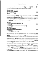
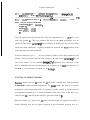
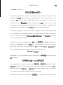
term or formula For example, the rule for assignment to a whole variable is:
P aEva yn Znrmgc(y, type(x)) A QIr
---------------------------1-1P Ex := yJ Q
Consider a typical context:
TYPE. s= 1.500;
VAR g:s; h:INTEGER;
...
9 := h+4;
Since g is a subrange variable, the assignment statement will cause a subrange error
unless h+4 is in the correct range. Znrange(y, type(x)) is the notation for a formula
which asserts that the value of y is in the range of the variable x. In the example
Notation for the extended semantics
11
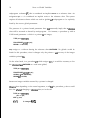
context, the desired instance of the rule is:
P [rEval h+4n 1 sh+4 A h+45500 A Q g
I - - - - - - - - - - - - - - - - - - - - - - - - - - - - - - - - - - - - I-h+4
-p ag := h+4n Q
2.8 Formula Constructing Functions
Inrange(<expression>, <type>)
Inrange is a function mapping <expression> x <type> + <formulal>. The expression
must be of a sort which covers the type.
if type is a subrange a..b,
Inrange(expression, type) +
alexpression
A
expressionlb.
otherwise,
Inrange(expression, type) + TRUE.
Dis joint( <Pascal variable>, <Pascal variable>)
The function Disjoint maps a pair of Pascal variables into a formula1 which is true iff
the variables are disjoint. Refer to Appendix B for a detailed definition of Disjoint.
Dis joint-set( <set of Pascal variables>)
For any finite set of Pascal variables, Disjoint-set constructs a formula1 which is true iff
all pairs of variables in the set are disjoint.
3. Theory of Definedness: The Predicate DEF
In order to introduce the possibility that a program variable can be uninitialized, we
12
Theory of Definedness: The Predicate DEF
assume the existence of an uninitialized scalar value, Q. The value of a newly created
program variable is unspecified. (This is explained more fully in section 6.3.) Before
the program can use the value of a variable, it must assign the variable a fully
initialized value: one such that none of its components is equal to fl. The predicate DEF
will be true only of these fully initialized values
In the intended model of the first order theory of DEF, terms of a simple sort range
over a universe of values including n. Values of compound sorts are built up by using
the sets of simple values as components. For example, the possible values of a variable
of sort ARRAYkl OF INTEGER include arrays with some positions equal to n.
Axioms DEFl-DEFS below describe the properties of DEF and of Pascal types.
DEFl) for every constant c, DEF(c) is an axiom.
DEF2) if e is of an enumerated sort (cl, . . . ,cn),
DEF(e) 3 e=clv . . . ve=cn.
DEF3a) if x is an expression of sort ARRAY[a..bl OF t,
DEF(x) E (Vi a<i&b 3 DEF(x[il)).
DEFSb) if r is of a Pascal record sort, and f 1, . . . ,fn are the record field names,
DEF(r) I DEF(r.fl )A . . . ADEF(r.fn).
DEF3c) if #t is of a reference class sort,
DEF(#t) = (Vp B POINTERSTO( (p#NIL = DEF(#tcp$).
DEF4) DEF(a)ADEF(b) 2 DEF(a @ b)
where 8 is an operator in {+, -, $, =, 2, <, I, AND, OR, NOT}
DEFS) DEF(a)ADEF(b)AbO 2 DEF(a/b)ADEF(a DIV b)ADEF(a MOD b)
Axiom DEF6 defines equality for compound types: ,
DEF6a) if x and y are expressions of a record sort, and f 1, . . . ,fn are the field names,
x=y 1 (x.fl =y.f 1 A . . . A x.fn=y.fn).
DEF6b) if x and y are expressions of sort ARRAY[a..bl OF t,
x=y s (Vi al&b =) x[i]=y[i]).
The following two axioms are not normally needed for proving absence of runtime
errors in programs, but are included for thoroughness:
Theory of Definedness: The Predicate DEF
13
DEF7) for each sort3 s, (3Xs -DEF(X,)) is an axiom, where Xs is a variable of sort s.
Axiom DEFS states that the result of selecting a component of an array or reference
class using an undefined or out of range index is not DEF.
DEF8a) if x is of sort ARRAY[a..bl of t,
DEF(x[i]) I> a<iAilb.
DEF8b) if #t is of a reference class sort,
DEF(#tcp$ =) DEF(~)A~~NIL.
The resulting theory of DEF is still not logically complete, e.g. because it does not say
much about the undefined values. But we should not expect to find such details in a
programming language definition. All of the properties needed for proving absence of
errors in programs have been included.
3.1ConsistencyofthetheoriesofDEFanddatatypes.
Each sort has some standard properties which must be included in the complete logical
system. Proofs involving the integer sort appeal to the usual properties of integers etc.
In the extended semantics, each sort ranges over a universe including some uninitialized
values. This section is concerned with the question of how the presence of uninitialized
values affects the theories of the sorts. One problem that could potentially arise is that
the standard properties associated with a sort could imply that all its elements are DEF,
contradicting axiom DEF’7.
Consider the conjunction of axioms DEFl and DEF7. Axiom DEFl says that every
constant symbol in the language corresponds to an initialized value. Axiom DEF7
asserts that there are values for which DEF is false. Obviously, these values cannot be
named constants or terms built from constants. This raises the questions of consistency
and of what the models of the sorts are like. In the extended semantics, each sort must
3 except for array sorts with no components, such at ARRAY[l..O] OF t.
14
Consistency of the theories of DEF and datatypes.
.
have a theory whose models contain at least one unnamed element. This requirement is
easily satisfied, but it must be taken into account in choosing axioms for each sort. For
instance, axiom DEF2 permits the models of enumerated sorts to contain extra elements
which are not DEF. Consequently, all finite simple and compound sorts have extra
elements that are not DEF.
The extended semantics is intended to be used with a “standard” theory of the integers,
and with standard theories of data structures with the selection and assignment
operations [I 11. Each of these theories has a standard model containing only the values
for which DEF is true in the extended semantics.
It would be possiole to assure the
consistency of the combined theories by restricting the axiomatization of data structures
to values for which DEF is true. Under this approach, if Vx P(x), is a standard axiom
for a certain sort, then Vx DEF(x)2P(x), would be chosen as the corresponding axiom in
The obvious disadvantages of this approach are that the
the extended semantics.
axioms are more complicated and proofs would have to establish the truth of DEF for
every term in order to apply sort axioms.
We would like the extended semantics to
have the same sort axioms as the ordinary system, so we choose to use the standard
axioms of data structures and to take advantage of the existence of nonstandard models.
For instance, since all of the standard integers have constant symbols, the models of our
integer sort under the DEF axioms are the nonstandard models of arithmetic -- models
with extra elements.
There is only one point that requires some care, and that is
combining the theories of DEF and arithmetic. The “standard” theory of arithmetic
must not contain the symbol DEF. If an axiom system for arithmetic is used, it must not
contain DEF. For example, if the axiom system has an induction schema, instances
involving DEF cannot be used. Without this precaution, the axioms would give a
contradiction. Suppose that the induction scheme for integers is
a(O)
A
( V n a(n) 3 Q(n-l)AO(n+l)) 2 (Vx a(x)).
(W
Then from DEF(0) and DEF(n) 3 DEF(n-l)ADEF(n+l) one could deduce Vx DEF(x),
which contradicts axiom DEF7.
Consistency of the theories of DEF and datatypes.
15
Another approach is to use a special axiomatization of arithmetic that allows instances
with DEF. One such scheme for induction on the integer sort is:
e(O)
A
( V n @(n) 2 @(n-l)d(n+l)) 3 ( V x DEF(x) =) 4(x)).
(S-PI
3.2 The relationship between DEF and Inrange
In Pascal, every subrange type is bounded by two constants: ab. Thus according to the
definition of Inrange, Inrange(x, s) implies DEF(x), if s is a subrange. This follows from
t,he properties of the I ordering of the integers. For example, it is a theorem in the
theories of integer ordering and DEF that
V x (15x
A
x14) 3 DEF(x),
because the standard properties of integer ordering imply that
vX(l<XA
x14)3(X=1 V X=2
V
X=3
V
X=4)
and each of these constants is DEF. Note, however, that
‘dxvyvz (DEF(x)
A
OEF(z)
A
xSy
A
ye) 3 DEF(y)
(3.1)
is not a theorem about DEF, because it cannot be proven from S-P, the special form of
induction on the integers. Indeed, there are nonstandard interpretations of the theories
of DEF and integers for which formula 3.1 is not satisfied.
Also note that it is not necessary for a variable to be Inrange if it is DEF: under the
axioms of DEF, there can be a variable of a declared subrange type, whose value is both
DEF and not Inrange.
In the definition of P EAJ Q no program is permitted to assign a
value to a subrange variable unless the value is Inrange. If P [A] Q holds, a subrange
variable can only be out of bounds before it has been assigned a value.
4 Mom flaxibb bqpgos arm d’-d in section ?k
Fundamental inference rules.
16
4. Fundamental inference rules.
The following two rules are included in both the unextended and extended definitions:
(CONCAT)
Concatenation of programs.
P {A) Q, Q {B} R
---------------w--
PuAnQ, QibnR
------B-----I---I-
P {A; B} R
P IA; B] R
(CONSEQ)
Consequence rule.
PDQ, Q {A) R, RDS
------------I-----
PDQ, Q EAl R, RDS
1-------1--------1
p CA? s
p BAD s
These rules will be used implicitly, beginning in the next section on the semantics of
expression evafuation. Later, after P EA] Q has been defined, we will develop its logical
relationship to P {A} Q in more detail.
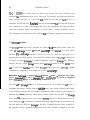
5. Expression Evaluation.
This section introduces and defines evaluation statements. Evaluation statements have
the forms
Eva1 <Pascal expression>
Locate <Pascal variable>
and in the extended semantics, they can be combined with Pascal statements and
assertion statements to form the general statements which appear inside brackets in a
formula P [An Q Evaluation statements will be used in section 6 to define the
conditions for error free execution of Pascal statements containing expressions and
variables.
The statement Eval E, corresponds to the action of evaluating the expression E, which
Expression Evaluation.
may not have side effects.
17
P [EvaI EI] Q is defined to mean that if P holds, then E
evaluates without runtime error, and if E terminates then Q will hold. Since E does not
have side effects, P and Qrefer to states with the same values for variables. By having
two assertions, it is possible to make partial correctness statements about function calls.
For instance, if f is a (strictly) partial function,
Nx> [Eva1 fwn Qh, f(x))
may be a provably true statement about the evaluation of f(x), while the pure first order
statement
P(x) = Qb, f(x))
would not be true since it does not account for divergence of f(x).
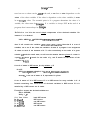
The other form of evaluation statement, Locate V, corresponds to the action of
computing the location of a variable. The difference between this and evaluating a
variable is that to compute a location, all of the subscripts must be evaluated and all
dereferenced pointers must be evaluated, but the variable itself need not have a value.
For instance, to execute the assignment statement A[j]:=e, the subscript j must have a
value in the correct range, but the left hand side A[j] is not required to have a value.
The definition of A[j]:=e is expressed in terms of Locate A[j], and Eva1 e, since the
right hand side must yield a value. The formula P KLocate W] Q is defined to mean
that if P is true, then the location of V can be computed without execution errors, and if
the computation terminates, Q will hold.
The exact meaning of expression
e v a l u a t i o n i s often a point of c o n f u s i o n i n
programming languages and definitions. The definitions presented here assume that
sufficient restrictions are used to prevent side effects. Pascal 191 assumes a fixed order
of evaluation within statements and expressions, so the final value of an expression is
well determined even in the presence of side effects. It is a simple matter to replace a
function definition which has side effects by an equivalent procedure definition, by
adding a new VAR parameter to return the function value. Thus it is possible to
18
Expression Evaluation.
rewrite a Pascal program in which functions have side effects into an equivalent
program in which function calls are replaced by procedure calls and all expressions are
free of side effects. This transformation would convert the evaluation of an expression
with side effects into a sequence of procedure calls involving some new variables to
store temporary values. Since this transformation can be easily mechanized, our Pascal
semantics are indirectly applicable even to programs with function side effects.
If runtime errors are not being considered, as in the original Hoare axiom system,
function calls without side effects can be defined by the following rule,
$(X1, . . * ,Xn,G) {Function f(X1 :tl ; . . . ;Xn:tn):tf; B) Of(X1, . . . ,Xn,G),
P {Eval Al; . . e ;Eval An) If(A1, . . . ,An,G) A (Of(Al, . . . ,An,G) 2 Q)
-----------------------------------------------------------~P {Eval f(A1, . . . ,An)} Q
which states that evaluation of f(A 1, . . . ,An) can be reduced to the evaluation of
A l , . . . ,An in order, followed by the application of f, if If and Of are shown to be
valid entry and exit assertions for f. G is the set of read only global variables, and B is
the body of the function f.
A fine point to be considered at the practical level is that some compilers change the
order of evaluation within expressions if there are no side effects. If the evaluation of
an expression terminates, it terminates with the same result under all orderings. Since
the truth of P (Eva1 E) Q depends only on whether evaluation of E terminates and the
value of each subexpression, all orders of evaluation are equivalent with respect to
P {Eval E) Q The truth of P {Eval E) Q can be determined by choosing any possible
ordering and considering whether it is true for that ordering. Rule Fl above, depends
on choosing one ordering. Thus Fl is correct even if there is reordering.
The situation is different when proving absence of runtime errors. Then, different
possible orders of evaluation must be considered separately. For instance, an expression
such as f(x)+a[i] might have a runtime error if i is out of range. If f(x) is evaluated
first and does not terminate, the error cannot occur. But if the order is changed and a[i]
Expression Evaluation.
19
is evaluated first, the error could occur. Since different orders of evaluation can give
different results, we define P EEval En Q to be true iff every order of execution is error
free and Q will hold after every terminating execution.
Another complication is the possibility of short circuit evaluation in Boolean expressions.
In evaluating an expression such as r AND s, when the value of r is False, Pascal permits
compilers to omit the evaluation of s. The expression r AND s is assumed to have the
value False because r is False. Observe that if s does not terminate or if it has a
runtime error, the short circuit has a different partial correctness semantics from full
evaluation. For example,
P [EvaI r AND sn False
may be true for full evaluation but not for short circuit. Short circuit evaluation is
really a form of branching within expressions. The axiomatic definition assumes that
full evaluation is used. Some languages, such as ADA, permit short circuit evaluation in
certain contexts but require the user to explicitly request it. This seems to be a cleaner
approach, and we show below (rule E3S) how it can be formalized in the extended
semantics.
In summary, our detailed semantic definition of Pascal statements will be based on
partial correctness assertions about evaluation of expressions and variables. It is argued
that even in the absence of side effects, the definition of expression evaluation should as
a practical matter account for possible variations in the order of evaluation. We will
give an axiomatic definition that does not assume any fixed ordering. On the other
hand, function call rule Fl can be used if evaluation order is fixed, or if runtime errors
are not considered.
The rules defining P [EvaI en Q are as follows:
20
Expression Evaluation.
Expression evaluation.
P KLocate Vl] OEF(V) A Q
---------------------o-o
P [Eva1 VI Q
(V is any Pascal variable.)
P BEval A] Q
--------o------------o-
033
P &val (@ A)I] Q
(where @ is one of the monadic operators, +, -, NOT)
The following rule for evaluation of an operator expression contains three conditions.
The first two assert that A and B evaluate without runtime error if P holds. These
conditions make the rule independent of any fixed order of evaluation, by requiring
either operand to evaluate correctly if evaluated first. The third condition states that
after both operands have been evaluated, Q must hold. Since there are no side effects
and the first two conditions have established that the operands evaluate without errors,
the order in the third condition is not significant. Notice, though, that the first
condition is redundant because the third one also requires A to evaluate safely. In
stating the rest of the rules, we will omit redundant conditions such as this.
P [EvaI A] True,
P IEva Bl] True,
P IEva A; Eval Bj’j Q
e-----------------o-
(E3)
P [EvaI A@Bn Q
(where @ is a relation sign or boolean connective.)
Rule E3S formalizes evaluation of ADA conditions. In ADA, the boolean conditions for
controlling IF and WHILE statements etc. can have one of the forms
<expression> AND THEN <expression>
<expression> OR ELSE <expression>
which indicate that the left hand expression is to be evaluated first, after which the
right hand expression will be evaluated only if its value is needed to determine the
value of the condition. The following rule for evaluation of A AND THEN B states that it
Expression Evaluation.
21
must always be possible to evaluate A, and that 1) if A is false, Qmust hold, and 2) if
A is true, it must be possible to evaluate B, after which Qmust hold.
P [Evai AI] -A 3 Q,
P [EvaI A; ASSUME A; Eva1 B] Q
------I-----_------_----------
E3S)
P EEval A AND THEN B] Q
Maxint is an undeclared integer variable representing the range on which integer
arithmetic operators do not overflow.
The axiomatic definition makes no assumption
a b o u t the values of Maxint. In order to prove absence of overflow, the user m u s t
supply assertions relating Maxint to the computations in the program.
P EEval Bg True,
P [rEval A; Eva1 Bn -MAXINTsA@BsMAXINT
--------------------_________I__________-
A
Q
P [rEval AeB’Il Q
(where $ is one of the arithmetic operators, +, -, *:)
P EEval BJ True,
P IfEval A; Eva1 Bj &O A Q
------------------*----------------------
E5)
P [EvaI A@Bn Q
(where @ is DIV, MOD, or 1)
Maxint can have any value such that integer arithmetic does not overflow in the range
-Maxint . . Maxint Note that many computers use twos complement arithmetic, in which
the smallest negative integer has an absolute value one greater than the largest positive
integer. This situation (and other possible number systems with asymmetrical ranges)
can be more accurately modeled by introducing a separate variable Minint to stand for
the smallest integer, and making the obvious changes in rules E2, E4, and E5.
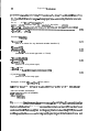
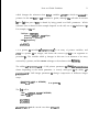
The following rule defines the evaluation of a function call f(A1, . . . ,An), where each of
the Ai is a value parameter and C is a list of read only global variables. For error free
evaluation of the function call, each of the Ai must evaluate and yield a value in the
proper range.
The second the third premises of the rule state that if If and Of are
valid entry and exit assertions for f, then they can be used to show NEval f(A)m If the
22
Expression Evaluation.
parameters A and G satisfy the entry condition If, then Of will hold on exit. Also,
f(A,G) will be DEF and Inrange -- these properties are assured by the declaration rule.
for i=l, . . . ,n, P UEval Ail] Inrange(Ai, ti),
If(X1, . . . ,Xn,G) {Function f(X1 :ti; . . . ;Xn:tn):tf; B} Of(X1, . . . ,Xn,G),
P [EvaI Al ; . . . ;Eval An] If(A,G) A (Of(A,G) A DEF(f(A,G)) A Inrange(f(A,G), tf) => Q)
~~~~~~~~~-~~~~~~~~-~~~~~~~~~~~~~~~~~~~~~~~~~~-~~~~~~~-~~~~~~~-~~~~~~~~~~~~~~~~~
P UEval f(A1, . . . ,An)B Q
E6)
Location Validlity.
(L1)
P ULocate VJ P
(this is an axiom for any declared variable identifier V)
I
I
P BLocate Rn Q
c--------------P [Locate RF] Q
(where R is of a record type with a .F field)
(La
P UEval Zl] ZzNIL A Q
1--1----------------
O-3)
P ULocate Ztn Q
(where Z is of a pointer type)
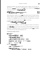
P UEval I] True,
P [Locate A; Eva1 a Znrange(1, indextype( A Q
(14)
-------------------------------------------------------
. P [Locate A[Ifl Q
(where A is of an array type)
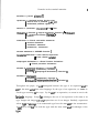
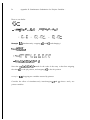
Example 2: Show Q UEval a[i]+pll] True, where
Q E DEF(i)
A
Olill 0 0
A
DEF(a[i])
A
01a[i]l25
A
DEF(p)
A
pirNIL
A
pl=6
A
1 OOOIMAXINT
with the variable declarations
V/AR a: ARRAY[O:l 001 OF INTEGER;
VAR i: INTEGER;
VAR p: HNTEGER;
By a p p l y i n g the inference rules in reverse, we can find simpler sufficient conditions for
the formula to be true. W e w i l l continue to work backwards until we reach sufficient
conditions that are obviously true. At this point, the formula will be proven, because it
will be possible to construct a formal proof by starting with the final conditions md
Expression Evaluation.
23
applying the inference rules until the original formula is deduced. The first step is to
use rule E4 in reverse, reducing the problem of proving a statement about Eva1 a[i]+pT
to proving statements about Eva1 a[i] and Eva1 p7.
Q KEval ptn True,
and Q EEval a[i]; Eva1 pt] -MAXINT I a[il+pt 5 MAXINT.
(5*1)
(5.2)
Before finishing the example, we pause to mention a fact about the extended semantics
which is helpful in removing redundancy from proofs. Since expressions do not have
side effects, we can assume in proofs that the state does not change when an expression
is evaluated. The following lemma states this fact in a useful form.
Lemma. t- P [EvaI eD True, lff l- P UEval en P.
t- P [Locate efl True, iff l- P BLocate en P.
Another point about redundancy is that when applying the inference rules directly to
prove P UEval EI] GI, the proof of error free execution of some subexpressions may appear
many times. A mechanical evaluator of the preconditions can easily take the repetition
into account and only verify each subexpression once.
Continuing the example, show 5.1:
Q lfEval ptn True
+ QULocate ptn DEF(pt)
c Q UEval p] ~wNIL
A
DEF(pt)
c Q BLocate pl DEF(p)
c Q 2 (DEF(p)
t True.
A
p#NIL
(by El)
A
(by L3)
prNIL
A
DEF(pt)
(by El)
(by Ll and CONSEQ)
A DEF(pW
(by definition of Q)
Next, show Q IEva aria True
t Q [Locate aria DEF(aCi1)
(by El)
t Q UEval i] DEF(aCil),
a n d Q BLocate A; Evai in 0% 100
A
DEF(aJll)
(by L4)
Expression Evaluation.
24
These last two formulas are trivially provable, since the assertion Qimplies that i has a
value, and the whole variable A is always a valid location by Ll. Having shown that
both di] and pr evaluate without any errors, we can use the CONCAT rule to infer that
one can be evaluated after the other, i.e.
Q {Eval a[i]; Eva1 pT) T r u e
(by CONCAT).
t5*3)
It only remains to show that there is no overflow, formula 5.2.
Q {Eval a[i]; Eva1 pl) -MAXINT I a[il+pt 5 MAXINT
t Q 2 -MAXINT I a(i]+pt I MAXINT
(by CONSEQ and Iemma applied to 5.3)
+ True.
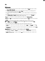
Example 3: User defined partial functions in expressions.
VAR x: INTEGER;
VAR a: ARRAY[O:lOOl OF BOOLEAN;
FUNCTION sqrt(n: INTEGER): INTEGER;
ENTRY True;
EXIT Olsqrtln
BEGIN
X if n < 0, then loop forever without execution errors;
otherwise, set sqrt t integer part of square root n.
x
Suppose the function sqrt has been defined to correctly return the integer square root
of n unless n is negative, in which case it loops forever without runtime errors. Using
the function declaration rule which will be given in section 6.3, it is possible to prove
True UFunction sqrt(n:INTEGER):INTEGER;
body3 Olsqrt(n)ln.
(5.4)
The entry and exit specifications of sqrt can then be used to show that if sqrt is called
with an argument x whose value is less than 100, the location of the variable a[sqrt(x)]
can be computed without runtime error.
Expression Evaluation.
DEF(x)
A
25
xl1 00 BLocate a[sqrt(x)a True
t DEF(x)
A
(5.5)
xl1 00 lfEvai sqrt(x)l) T r u e ,
and DEF(x)
A
xl1 00 Ilocate a; Eva1 sqrt(x)] Olsqrt(x)ll 00
(by L4)
(5.6)
Using the function call rule E6, the first part 5.5 reduces to
DEF(x) A ~5100 UEval sqrt(x)n True
t DEF(x)
A
xl1 00 [Eva1 xl T r u e ,
and True IFunction sqrt(n:INTEGER): INTEGER; body1 Orsqrt(x)lx,
and DEF(x)
A
xl1 00 UEval x3 True
A
{Olsqrt(x)<x
A
DEF(sqrt(x)) 2 True)
which are all true.
The second part 5.6 can be simplified
DEF(x)
A
xl1 00 [[Locate a; Eva1 sqrt(x)] Olsqrt(x)ll 00
t DEF(x)
A
xl1 00 [EvaI sqrt(x)l] Olsqrt(x)slOO ( b y Ll a n d CONCAT)
t DEF(x) A x< 100 UEval xl (Olsqrt(x)lx
(by EN
t OEF(x) A x,< 100
BLocate xn DEF(x)
(by El)
A
(Olsqrt(x)lx
t DEF(x) A xl1 0 0 3 DEF(x)
(by Ll and CONSEQ)
A
A
A
D E F ( s q r t ( x ) ) 3 Olsqrt(x)s 100)
DEF(sqrt(x)) =) Olsqrt(x)<lOO)
(Olsqrt(x)lx
A
DEF(sqrt(x)) 3 Olsqrt(x)llOO)
+ True
6. Extended axiomatic semantics of Pascal
6.1 Assume statements
The meaning of the statement ASSUME L, is that L can be assumed to be a true assertion
Assume statements
26
at a certain point in a program. Assume statements do not initially appear in programs,
but can be introduced during the course of a proof to record logical assumptions which
hold at points within a program.
For instance, the rule for IF statements reduces a
formula involving IF L THEN Sl ELSE S2 to two formulas for the two cases of the
condition L. In one formula, the statement ASSUME L records the assumption that L was
true, and in the other formula, ASSUME -L records the assumption that L was false.
(PAL) 2 Q
--------------P
( ASSU M E )
~ASSUME L] Q
6.2 Executable statements
Assignment statements
The following rule applies to all assignment statements.
P EEval en True,
P KLocate pv; Eva1 el] Inrmge(e, type(pv)) A Qly
----------------_---------------------------------------
(ASSIGN)
p Ifpv := e]Q
where pv is any Pascal variable
In order for P upv := en Q to hold, it is necessary for the assignment to execute without
any runtime errors, and for Q to be true in the updated state. The rule requires the
right hand side, e, to evaluate without runtime error and to yield an initialized value;
the location calculation for left hand side pv is also required to be free from errors. If
pv is a subrange variable, the Inrange clause requires the value of e to be in the correct
range. The updated formula Q is formed by substituting e for the Pascal variable pv,
using the definition of substitution given in section 2.2.
Executable statements
27
IF statements
P IEva L; ASSUME L; Sll) Q,
P KEval L; A S S U M E -L; S23] a
-----------------------------
(IFI
P KIF L THEN Sl ELSE 5211 Q
CASE statements
for i=l, . . . ,n, P IEva X; ASSUME X=Ci; Sd Q,
P [EvaI Xl Xc{Cl, . . . ,Cn)
-------------_--------I----------------------------P EcASE x 0F cl :sl; . . . ;c,:sJ Q
(CASE)
The Ci are lists of constants for each branch of the CASE statement. The second
condition requires the CASE expression X to evaluate to one of the constants in one of
the Ci.
NEW procedure
The following axiom states that the effect of the Pascal statement NEW(x), where x is a
variable identifier of a pointer type, is to change the value of x to a new pointer value
xo, and to add the new value xo to the reference class.
-(x0 c P O I N T E R S T O (
where x
x0
#T
#T
A
DEF(x0)
A
x&NIL 2
Q
I
QT
x [rNEW(x)n Q (NEWl)
#T u (x03 I x0
is an identifier of type tT (pointer to object of type T),
is a fresh identifier not appearing in Q,
is the reference class for type T,
u {x0) stands for the reference class after adding an object pointed to by x0.
The antecedents on the left side of the rule state that 1) the value x0 generated by NEW
is a new pointer, not a pointer to the reference class #T, 2) x0 has an initialized value,
and 3) x0 is not the pointer NIL. The term #T u {x0} represents the new reference class
after the dynamic variable xOt has been allocated. A more complete discussion of
POINTERSTO and the operation of adding new elements to a reference class can be found
in Ill].
Executable statements
28
The following rule reduces a NEW statement involving a selected variable to a NEW
statement with an argument which is an identifier.
P [NEw(so); S:=S0n Q
---------I--“----------
(NEW2)
P [NEW(S)n Q
where SO is a new identifier not appearing in the scope, P, or Q.
the declaration VAR SO: type(S) is added to the scope.
WHILE statements
P 2 I,
r [EvaI 6; ASSUME 8; Sn I,
I BEval Bn -B 3 Q
--------------------___________
P [I N V A R I A N T I
WHILE B DO
(WHILE 1)
Sn Q
fn this rule, the invariant is chosen to be true before each evaluation of the While test
B. The rule can be rearranged to correspond to other choices of invariants.
6.3 Functions and procedures
6.3.1 Function declaration
With the function declaration rule, one can infer that I and 0 are valid entry exit
specifications for a function f, if for inputs satisfying I, the body of the function
executes without runtime errors and assigns a final value to the function which satisfies
the exit assertion 0.
Function declaration
1(X1, . . . ,Xn,G) A DEF(X1 )A . . . nDEF(Xn) A hfange(X1 ,tl)~ . . . tinrange(Xn,tn)
KBJ O(f,Xl, . . . ,Xn,G) A DEF(f) A Inrange(f, tf)
-------------------------------------------------------------------------------I(X1, . . . ,Xn,G) [Function f(X1 :tl ; . . . ;Xn:tn):tf; BB O(f(X1, . . . ,Xn),Xl, . . . ,Xn,G)
29
(FD)
where f has the function declaration
FUNCTION f(X1 :tl; . . . ;Xn:tn):tf;
GLOBAL G;
ENTRY 1(X1, . . . ,Xn,G);
EXIT O(f,Xl, . . . ,Xn,G);
B;
The rule requires that the function have only value parameters Xl, . . . ,Xn and a set of
read only globals G.
The rule assumes that each of the value parameters has an
initialized value in the correct range; this assumption is justified by the call rule, which
checks the actual parameters. If global variables are accessed, the entry assertion must
assert that they have been initialized.
In the exit assertion O(f,X 1, . . . ,Xn), the variable f stands for the value returned by the
function. The rule checks that the body assigns f a value in the correct range. As we
will see in section 7.4, the condition Inrange(f, tf) appearing after execution of the
body is redundant. Because the declaration rule requires f to be DEF after execution of
the body, it is not necessary to require f to be Inrange.
6.3.2 Note on Global Variables
Runcheck requires the user to declare lists of all global variables that could potentially
be accessed or altered by each subprogram. The system checks the lists by a syntactic
examination of the subprogram body. For instance, a global variable g which is used in
an assignment statement g := e, must be declared read write. Also, if the body of p
contains calls to q, then all globals listed for q must be listed for p.
Reference classes are a special case of global variables which are implicitly accessed or
altered although they do not appear explicitly in the executable program text. If a
30
Note on Global Variables
subprogram evaluates pr, this is considered an implicit access to a reference class. An
assignment pt := e is considered an implicit write to the reference class. The system
requires all reference classes which are used as globals of a subprogram to be explicitly
listed by the user as global parameters.
The presence of a pointer formal parameter does not necessarily imply that a reference
class will be accessed or altered by a subprogram.
For instance, a procedure p with a
VAR formal parameter x which is a pointer to an integer,
TYPE ptr = tINTEGER;
PROCEDURE p(VAR x: ptr);
BEGIN x := NIL END;
may assign to x without altering the reference class #INTEGER. No globals would be
listed for this procedure, since it changes only the pointer x and not any of the integer
variables pointed to.
On the other hand, in a procedure p2 which assigns to xt, it would be necessary to list
the reference class #INTEGER as a read write global,
TYPE ptr = IINTEGER;
PROCEDURE p2(VAR x: ptr);
GLOBAL (VAR #INTEGER);
BEGIN xt := 0 END;
because an integer variable accessed by a pointer is changed.
Observe that depending on the actual argument, a call to the procedure p above could
have the effect of changing a reference class, as in the call
TYPE ptr = tINTEGER;
ptr2 = tptr;
VAR y: ptr2;
P(YV;
% changes #ptr %
Note on Global Variables
31
which changes the reference class #ptr of variables of type ptr which are accessed by
pointers. In this case #ptr is not considered a global, although the call rules do account
for the fact that part of #ptr is altered by being passed as a VAR parameter. Which
reference class is altered in this example depends on the call, not on the definition of p.
For example, in the call
TYPE ptr = tINTEGER;
ptrarray = ARRAYS 1 ..l 001 OF ptr;
ptrptrarray = tptrarray;
VAR z: ptrptrarray:
z is a pointer to variables of type ptrarray, z7 is an array of pointer variables, and
zr[SO] is a pointer to an integer, and hence the correct type to be an argument to
procedure p. The variable which p changes in this case is an element of an array
accessed by a pointer, and this causes a change to the reference class #ptrarray.
The ability of a procedure with a VAR pointer parameter to change different reference
classes depending on the actual parameter, is exactly analogous to the ability of a
procedure with a VAR integer parameter to change components of different integer
arrays.
PROCEDURE q(VAR x: INTEGER);
BEGIN x:= 0 END;
% no giobais %
The first call in
TYPE arr = ARRAY11 ..5001 OF INTEGER;
VAR vl, v2: arr;
qw cm);
qwc~o1);
alters part of vl, but the second one alters part of ~2.
Procedure declaration
32
6.3.3 Procedure declaration
I(X,Y,G) A DEF(X1 )A . . . ADEF(Xm)
A hrange(Xl,tl)~ . . . nhrange(Xm,tm)
EBn OWXG)
-_-------------_----______l____________l--------------------------------------
U’D)
I(X,Y,G) I[Procedure p(X1 :tl; . . . ;Xm:tm; VAR Yl :ul ; . . . ; VAR Yn:un); Bn O(X,Y,G)
where p has the procedure deciaration
PROCEDURE p(X1 :tl ; . . . ;Xm:tm; VAR Yl :ul ; . . . ; VAR Yn:un);
GLOBAL GR, VAR GW;
ENTRY I(X,Y,G);
EXIT O(X,Y,G);
B;
GR are the readoniy global variables,
GW are the read write global variables,
G stands for the set of all global variables, GR u GW.
Like the function declaration rule, the procedure declaration rule assumes that the value
parameters are initialized by each call with values in the correct range On the other
hand, there is nothing unusual about procedures that work correctly with uninitialized
VAR parameters. Consider a simple procedure p which is called with an integer j and
two array variables, x and y, and assigns x[j] the value y[j].
TYPE s = 1 ..l 00;
TYPE arr = ARRAYIs OF INTEGER;
PROCEDURE p(j: s; VAR x, y: ad;
BEGIN
xCj1 := yCj1;
END;
Since the procedure does not test the range of j before executing the assignment, a call to
p will produce a subscripting error unless j is between 1 and 100. Also, the actual
variable supplied for y[j] must have been assigned a value before the call to p. No
other restrictions are needed to assure error free execution. In particular, p will work
regardless of whether x has been initialized, and regardless of whether portions of y
other than y[j] have been initialized.
without errors.
For instance, the following sequence executes
Procedure declaration
33
VAR a, b: arr;
VAR k: INTEGER;
BEGIN
k := 50;
b[k] := 1000;
ptk, a, bk
% now a[501 = 1000 %
END;
The behavior of p can be specified by providing it with entry and exit assertions.
TYPE s = 1 ..lOO;
TYPE arr = ARRAY[sl OF INTEGER;
PROCEDURE p(J: s; VAR x, y: arr);
INITIAL y = y0;
ENTRY DEF(y[jl);
EXIT y = y0 A x[jl = ycjl;
BEGIN
xCj1 := yCj1;
END;
The entry assertion states that y[j] has a value when p is called. Note that since j is a
value parameter with a subrange type, the declaration rule assumes that it will be
supplied with a value in the correct range -- this will be checked by the call rule. The
Initial statement simply introduces a new name y0 to stand for the initial value of y at
the time of entry to the procedure. The exit assertion states that the value of y is
unchanged, and that x[j] is equal to y[j].
To summarize the point of this example, all of the rules for subprograms assume that
value parameters must be supplied with initialized values in the correct range. This is
our interpretation of what it means to correctly call a subprogram with a value
parameter. No such assumption can be made for VAR parameters, and so it is
necessary to describe the behavior of each one by means of entry and exit assertions.
It is of course possible for there to be implementations of Pascal, in which calls with
value parameters will produce the desired results in some cases even if the actual
parameter is not fully initialized.
This is merely an artifact of certain possible
34
Procedure declaration
implementation techniques. Our definition attempts to capture what is meant by the
language itself, and is intended to be sufficiently restrictive to be consistent with all
possible implementations.
As was mentioned earlier, the initial value of local variables is not specified by the
function or procedure declaration rules. Another approach, which seems reasonable at
first glance, is to assert that every local is initially undefined. This is not needed in the
extended semantics, because for P [A]1 Q to be valid, every variable must be assigned a
value which is DEF before its value is used.
The declaration rules could be modified to specify an initial value for locals, but this
would unnecessarily complicate the definition and lead to confusion in applying the
extended semantics. It would be possible to introduce a new constant Cs for each sort to
stand for the initial value. The axioms would be changed to state that for each of these
constants, -DEF(C,), and also -DEF(t) for terms t formed by selecting components of C,
For each local L, L=C, would be added as a premiss in the declaration rule. But this is
an unnecessary complication. Also, it does not accurately model the implementation of
Pascal, in which initial values are left unspecified to reduce overhead. For this reason,
it would give confusing results in practice. If a program, A, never used two variables of
the same sort, x and y, and otherwise executed without errors, it would be possible to
prove that the variables were equal after the program,
P {A3 x=y.
Such a result differs from the implementation and probably conceals a programming
error.
6.3.4
Procedure call
The procedure call rule requires each value parameter to evaluate without runtime
Procedure call
35
.
error, yielding a value in the correct range, and each VAR parameter to yield a location
without runtime error.
for i=l,. . . ,m, P [EvaI Aij Znrange(Ai, ti),
for i=l, . . . ,n, P [CLocate Vi] True,
I(X,Y,G) (rprocedure p(X1 :tl; . . . ;Xm:tm; VAR Yl :ul; . . . ; VAR Yn:un); B] O(X,Y,G),
PO[EvalAl;... ;Eval Am; Locate Vl; . . . ;Locate Vn] Disjoint-set(V u G) A I(A,V,G)
A vz,Gw (o(A,Z,GR,GW) 3 GII”:, . . . “,“,,
------------------------------------------------------------------------P (rp(A1, . . . ,Am,Vl, . . . ,Vn)l Q
(pm
Each of the actual VAR parameters, Vi, must be a distinct Pascal variable not in GW.
Note that this definition depends on the definition of substitution when Vi is not an
identifier.
7. Metatheory of the extended definition
In this section, we discuss some properties of the extended definition which are helpful
in reducing the complexity of program specifications and the length of proofs.
By itself, the extended semantics is not a complete solution to the problem of verifying
the absence of common errors.
In practice, there are two main kinds of difficulty in
doing actual verifications. These practical difficulties were carefully considered in the
design of the Runcheck system.
The problem of redundancy in proofs is solved in Runcheck by a special simplifier
which efficiently eliminates redundant verification conditions.
A more serious problem is the need for lengthly, detailed specifications and inductive
assertions in programs.
Several distinct approaches are needed to deal with this
problem. In Appendix A, we discuss the derived WHILE rule, which shows how the
extended definition reduces the need for detailed documentation. The derived WHILE
rule and other rules are logically justified by certain simple properties of the theory of
36
Metatheory of the extended definition
the extended definition, which are presented in the remainder of this section.
7.1 Ordinary Semantics Lemma
Any specification provable in the extended definition is also provable in the ordinary
definition.
Lemma 7.1 If I- P KA] Q, then I- P {A) Q.
The significance of this lemma is that all specifications, even those involving DEF, are
theorems of the ordinary system. 5 The extended definition only places more restrictions
cm the allowable computations.
Consistency of the extended definition is a direct
consequence of this lemma
7.2 Specification lemma
When proving complicated specifications for a program, it is sometimes helpful to prove
the specifications without considering possible runtime errors, and then prove separately
that no errors occur. In this way, the details about runtime errors can be isolated in the
proof. The next lemma says that proofs in the extended definition can always be
factored in this manner.
Lemma 7.2 If I- P {A) Q, and J- Pl KAj Ql, then t- PAPS [TA] Q/\Ql.
The reason for this is that if both P {A) Q and Pl aA] Ql can be proven separately,
then it is always possible to combine the proofs to show PAPI [fl Q/\Ql.
The design of the automatic Documenter in Runcheck is based on this lemma The
5 In the case of built in procedures, it is necessary to choose slightly nonstandard definitions if the resulting system is to be
complsts with respect to specifications involving DEF. The “ordinary” system that we have in mind has axioms stating that the
r8eults of built in procedures such as READ rnd NEW srs DEF.
Specification lemma
37
documenter constructs inductive assertion@ that are valid in the ordinary semantics.
The assertions can then be assumed true in proofs in the extended semantics. Thus the
documenter does not have to consider possible runtime errors while constructing the
invariants.
7.3 LESSDEF lemma
One of the basic properties of the extended definition is that if P ES3 Q holds, S cannot
assign an uninitialized value to any variable.
Over any sequence of statements that
executes without runtime error, the extent of variable initialization cannot decrease.
LESSDEF(x, y), a prtiicate for two terms of the same sort, is defined to be true if y is at
least as completely initialized as x.
LDl) if x and y are of the same simple sort,
LESSDEF(x, y) = OEF(x)aDEF(y).
L02) if x and y are of the same record sort, and the field names are fl, . . . ,fn,
LESSDEF(x, y) = LESSDEF(x.f 1, y.f 1)~ . . . ALESSOEF(x.fn, y.fn).
LD3) if x and y are of sort ARRAY[a..bl OF t,
LESSDEF(x, y) = ( V j aljrb 3 LESSDEF(xCj1, ycjf)).
LD4) if x and y are of sort REFCLASS(t) for some t,
LESSDEF(x, y ) c (VpPOINTERSTO(x) LESSOEF(xcpq ycp~)).
The LESSDEF lemma says that for any variable in a program that executes without
errors, the final value will be at least as fully initialized as the initial value.
Lemma 7.3 If t- P [An True, and v is a declared variable identifier then,
I- P A v’=v [AD LESSDEF(v’, v)
where v’ is a new identifier not appearing in P, A, or the scope.
’ Refer to [2] for dstrib of ths documenter.
38
LESSDEF lemma
In Runcheck, the lemma is used to reduce the need for detailed assertions on loops and
procedures. If a variable is known to be DEF before entering a loop, it is not necessary
to state in the invariant that it continues to be DEF. Similar assertions about VAR
parameters can be omitted from procedure specifications.
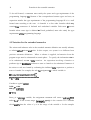
-ample 4: Merging two sorted arrays
This example shows how Runcheck uses the Lessdef lemma to reduce the need for
repetitious, detailed assertions. The program takes as input previously sorted arrays A
and B of length 100 and merges their contents into the array C, which has length 200.
The user has supplied only an ENTRY assertion saying that A and B are fully
initialized, and an EXIT assertion saying that C is fully initialized. The interesting
aspect of this example is that the initialization of C takes place in two loops. The first
loop partially initializes C, merging elements from A and B until either A or B has been
completely transferred. Then the initialization of C continues in either the second loop
or the third loop.
TYPE INARR=ARRAY[l : 1001 OF INTEGER;
TYPE OUTARR=ARRAY[ 1:2003 OF INTEGER;
VAR I,J,N:INTEGER;
VAR A,B:INARR; C:OUTARR;
ENTRY OEF(A)ADEF(B);
EXIT DEF( C);
BEGIN
N:=lOO;
I:=1 ;
J:=l ;
INVARIANT DEFRANGE( 7,Z+J-2, C)
A I<ZA ZgN+7 A 7sJ A JgN+7
WHILE (IIN) AND (JsN) 00
%EGIN
IF A[I]sB[Jl THEN BEGIN CCI+J-1 I:=ACII; I:=I+l EN0
ELSE BEGIN C[I+J-l]:=B[J]; J:=J+l END;
END;
Z’*Z;
INVARIANT DEFRANGE(Z’+N, Z+N- 1, C) A Z’<I h I,< N+7
WHILE IsN DO BEGIN C[I+N]:=A[I]; I:=I+l END;
J’CJ;
INVARIANT DEFRANGE(J’+N, J+N- 7, C) A JIgJ h J,(N+ 7
WHILE JsN DO BEGIN C[J+N]:=BtJ]; J:=J+l END;
END
LESSDEF lemma
39
The system will verify
DEF(A)
A
DEF( 8) Ibody DEF( C)
i.e., that the program does not have any execution errors and that no elements of C are
missed. All of the other variables are initialized before the first loop. Still, it is
necessary to prove that they are DEF each time they are accessed. In the case of a
variable such as I, Runcheck uses the Lessdef lemma to infer that it has a value
everywhere in the program after the assignment I:= 1. Even though I is changed on the
first loop, it is not necessary to write DEF(1) (or A, B, J, N) as an invariant.
In many array programs, the arrays are either supplied as fully initialized parameters,
or are initialized at the beginning. Without the Lessdef lemma, it would be necessary to
h a v e i n v a r i a n t s r e p e a t i n g the fact that an array or other data structure is DEF at
various points within a program.
Consider now the more complicated case of proving DEF(C). The system automatically
generates the statements shown in bold italics. By examining the first loop, one can see
that at any time, values have been assigned to the positions C[l], . . . ,C[I+J-21. This
fact is discovered by the system and is expressed in the invariant as
DEFRANGE( 1, I+&2, C).
DEFRANGE is a special predicate used to express that a subrange of an array is DEF.
Its definition is
DEFRANGE(x,y,a) P (Vi xl&y 2 DEF(aCi1)).
The invariant for the second loop states that C[I’+N], . . . ,C[I+N-I] are DEF, where I’
stands for the value of I before entering the second loop. Similarly, the assertion for the
third loop states that C[J’+N], . . . ,C[J+N-I] have been assigned values. The system
also produces the arithmetic inequalities shown on each loop.
To be able to prove the exit assertion, DEF(C), it is necessary to show that all of
40
LESSDEF lemma
C[l], . . . ,C[200] have values after the third loop. Notice that each invariant only
describes the initializations done by its own loop. For instance, the third invariant only
deals with the last part of C, and does not repeat the fact that the first part of C is
initialized by the first loop. Runcheck uses the Lessdef lemma to infer that the first part
of C continues to be DEF, even though that fact is not included in the later invariants.
Thus the invariants shown are sufficient to prove that C is fully initailized on exit.
The documenter’s assertions are also sufficient to show that the program executes safely.
7.4 lnrange lemma
The Inrange lemma says that a program for which P [AI] True holds cannot cause the
value of a subrange variable to become out of range (when started in a state which
satisfies P). If a subrange variable is known to always be DEF at some point in a
program that executes without errors, then the variable must be Inrange at that point.
To begin, we define Inrangsk, a formula constructor similar to Inrange. The difference
between the two is that Inrange asserts that a subrange variable is in the correct range
and is always true for other types, while Inranp asserts that every subrange variable
contained as a component of its argument is in the correct range.
Definition. Inrange* is a mapping <Pascal variable> x <type> + <formula>. For simple
t y p e s , Inrange*(v, t) is true if Inrange(v, t) is. Inrange*(v, t) is true for a compound
type if Inrange*(c, type(c)) is true for every component c of v.
The idea of the Inrange lemma is a characterization of the possible sets of states of
programs that always execute without runtime errors. Any actual execution must begin
in the outermost block with all variables uninitialized. Data needed by the program is
obtained by a READ procedure which always returns values that are DEF and Inrange.
Given that the program always runs without errors, what do we know about the set of
all possible states if it terminates? Variables that the program assigns to every time it is
run will always be DEF and Inrange* at the end. Variables that are never touched by
the program will be completely unspecified at the end. Variables assigned to on some
Inrange lemma
41
runs but not on others can be -DEF at the end, or can have a value dependent on the
values of the other variables. If the value is dependent on the other variables, it must
be an Inrang- value. The essential point is: If a program determines the value of a
variable, the value must be Inrange*.
If a variable is always DEF at the end of a
program, then it must always be Inrange*.
Definition. Let X be the set of simple components of the declared variables. For
instance if v is declared
VAR v: ARRAY CL.21 OF RECORD f:INTEGER; g:ROOtEAN END;
then X will contain the variables vC1 l.f, v(2l.f, v[l ].g, v12l.g. Note that X is a set of
variables, not a set of the values the variables. A state of a program is an assignment
of values to each of the elements of X. To refer conveniently to the value of a given
variable FX and the overall state, we will use the notation that the y-form of a state is
a pair <z,Z>, where z stands for the value of y, and Z stands for the values of the
variables in X-(y).
A set S of states is DEF-convex -for the- variable y, iff
for all Z,
(VZ <z,Z>cSy =) DEF(z)) implies (VW (w,Z>cSy = Znrangehw, type(y))).
where Sy is the set of states in S, represented in y-form.
A set of states of X is DEF-convex iff it is DEF-convex for every variable in X. A
formula containing free occurrences of declared variables is DEF-convex iff it is
satisfied by a DEF-convex set of states.
Examples: assume the declared variables are
VAR x: INTEGER;
VAR y: 1 ..l 0;
(7.1) True, False
(7.2) y=2
( 7 . 3 ) y=40
( 7 . 4 ) y*40
(7-5) DEF(y)
both DEF-convex
DEF-convex
not DEF-convex
DEF-convex
not DEF-convex
Inrange lemma
42
( 7 . 6 ) x=1 2 y=2
( 7 . 7 ) x=1 3 y=40
DEF-convex
not DEF-convex
If S is the set of final states of a program that does not have runtime errors, then S is
DEF-convex. In the examples, a program can set y to 2, so 7.2 is DEF-convex, but 7.3
cannot be DEF-convex because 40 is out of range. Although y+40 is DEF-convex, it is
not a possible set of final states - the DEF-convex sets include more than final states
sets. To attempt to characterize only final states would require much more detail than
we need here. Note that 7.5 is too weak to be a final set of states because it includes
both 7.2 (a possible set) and 7.3 (an impossible set).
Lenrma 7.4a If a program is started in a DEF-convex set of states and always
executes without runtime error, then the final set of states will be DEF-convex.
It follows that if a program always leaves a variable DEF when it halts, the variable
must be Inrange* at the end,
Lemma 7.4b If B is a Pascal statement, pv is a Pascal variable, P is a DEF-convex
predicate, and k P KB] DEF(pv), then i- P EBl Znrange*(pv, fype(pv)).
The restriction on P in this lemma is necessary. Recall that extended semantics does not
specify the initial values of variables, and that subrange type variables have the same
sort as the base type of the subrange.
Consequently, there is nothing that says a
subrange variable cannot be out of range if its value is not assigned by the program.
The following formula is a a theorem, even if the variable S declared with a subrange
of only L.100.
i- S=500 Bernpfyn DEF(S)
A
S=500.
Of course, the extended definition checks that any program that uses the value of S first
assigns it a value in the proper range.
Runcheck makes use of a restriction that the entry assertion for the outermost block of a
Inrange lemma
43
program must be DEF-convex.’ With this assumption, Runcheck can infer bounds on
the value of a subrange variable if it is known to be DEF. In some cases, this can
permit lengthly assertions to be omitted.
For instance, if a complex data structure
c o n t a i n s subrange variables and the entire data structure is D E F , b o u n d s for the
subrange variables can be deduced without any additional assertions. By induction on
the depth of procedure calls, the lemma can also be applied to formal parameters when
reasoning about a procedure body. Since a value parameter v must be DEF on entry,
Inrangti(v,t) must be true initially. Variable parameters do not have to be DEF on
entry, but if the value is used somewhere in a procedure body it must be possible to
prove that the variable is DEF and the Inrange lemma applies at that point.
Ehcample 5: Constructing a Spanning Tree.
The following program is a simple algorithm [ 121 for finding a spanning tree of an
undirected loop-free graph with E edges and V vertices. If the graph is disconnected, it
grows a spanning forest. The graph is entered as a table of edges in the arrays IA and
JA, so that the vertices of the kth edge are IA[k] and JA[k]. The program stores the
indices of the spanning tree’s edges in Till, . . . ,T[V-P], where P is set to the number of
trees in the spanning forest.
This example illustrates the use of subranges and the inrange lemma to strengthen the
entry assertion of a procedure. Since IA and JA are tables of vertices, they have been
declared as arrays of subrange values IV. It is typical in graph manipulating programs
to use a value stored in one array to compute an index into another array. Here, the
variable I is set to IA[K] and then VA[I] is accessed. For the latter access to be in the
subscript range 1:V of VA on every iteration, all elements of IA must have been in the
’ In m actwt Pasal program, no rssumptions an be m& &out tb initirl vrlues of vrrbbles decbrad in l outermost bbck. To
be strictly nrlistic, t)n vorifior should not permit ontry rssortions thora. Thv are permitted as I smrll convanianco;
l mrin bkxk
with an entry wtion is constirud to b a shorthand for 8 procedure with gbbals. The signifiunco of this is thrt the truth of
the entry rrrsortion must be rssurod by some ailing program i.e. it is possible to decbre l procedure with rn entry msartion that
is not DEF-comnx, but its rctwl wt of entry strtos is thn l DEF-convex restriction of the dacbred entry condition.
Inrange lemma
44
range initially. Because IA and JA are value parameters, their initial values must be
DEF, and by the inrange lemma, Runcheck can infer that the elements are in the correct
range. Similar reasoning is required for other array accesses.
VAR E,V:INTEGER;
PROCEDURE SPANNING(IA,JA: ARRAY[l :El OF 1 :V;
VAR P: INTEGER;
VAR T: ARRAY[l :V-11 OF INTEGER);
ENTRY DEF(E) A DEF(V) A 1sE A 2sV;
EXIT TRUE;
VAR I,J,K,C,N,R: INTEGER;
VAR VA: ARRAY[l :V] OF INTEGER;
BEGIN
c:=o;
N:=O;
FOR K:=l TO V ZNVARZANT I,<K A K,<V+I A DEFRANGE(I,K-&VA)
DO VA[K]:=O;
FOR K:=l TO E
I N V A R I A N T l,<K A K,<E+? A OSN A O,<C A N,<K-I A C,<K-I A K$V+N-1
DO BEGIN
IF K-N=V-1 THEN GOT0 1;
I: =IA[K];
J:=JA[K];
IF VA[I]=O THEN
BEGIN
T[K-N]:=K;
IF VA[J]=O THEN BEGIN
C:=C+l ;
VA[J]:=C;
VAtI]:=C;
END
ELSE VA[I]:=VA[JI;
END
ELSE IF VA[J]=O THEN
BEGIN
T[K-N]:=K; VA[J]:=VA[I];
END
ELSE IF VA[I&VA[JI THEN
BEGIN
T{K-N]:=K; I:=VA[I]; J:=VA[JI;
FOR R:=l TO V INVARIANT I,(t? A RgV+I
DO IF VA[R]=J THEN VA[R]:=I;
END
ELSE N:=N+l
END;
1: P:=V-E+N;
END;
Inrange lemma
45
Note that IA and JA could have been declared as arrays of INTEGER, and the restriction
on the values could have been part of the entry assertion. Expressing the restriction
would involve a quantified assertion such as
Vx (1 <xsE 2 1 <IA[xlsV).
This is both more difficult to write than the subrange type specification, and it causes
difficulty in theorem proving.
8. Generalizations of the extended semantics
8.1 Dynamic subranges
There are programming languages more flexible than Pascal, which allow declaration of
dynamic subranges.
ADA, in particular, has flexible dynamic type declarations. A
reasonable extension to Pascal is to permit subrange declarations involving expressions,
3
TYPE s = l..2*x;
The expressions for the bounds are evaluated each time the scope is entered, and the
range of s is fixed for the duration.
Dynamic arrays can be obtained by using a
dynamic subrange as the index type for an array etc.
The extended semantics can be adopted to handle dynamic subranges by defining
Inrange(e, s) to refer to the values obtained when the expressions for the bounds on s
are evaluated. The declaration rules for functions and procedures would be changed to
check for error free evaluation of the expressions in the type declarations. Also,
depending on the restrictions in the programming language, renaming would be needed
to distinguish between the initial values of the variables appearing in the type
declaration and the values assigned after the dynamic declaration was evaluated.
46
Bounds on depth of recursion and dynamic variable allocation
8.2 Bounds on depth of recursion and dynamic variable allocation
Like the bound for arithmetic overflow, bounds on recursion and heap storage are
implementation dependent. In critical applications, the actual bounds may be set in
advance, and one might want to verify that the available storage will be sufficient. In
other cases, the particular bound is not important, but it might be useful to verify that a
program does not attempt unlimited recursion etc.
To describe bounds on depth of calls, two new undeclared integer variables are
introduced in the procedure call rule. The variable Stksize represents the maximum
depth of calling; S t k p t r r e p r e s e n t s t h e current depth. The procedure call rule is
modified to enforce a restriction that StkptrlStksize. Neither variable can be assigned
to by the program. Stkptr is 0 on entry to a main program, and each level of function
or procedure calling increases it by 1. With these additions, the procedure call rule is
for i=l, . . . ,m, P (rEval Ail] Znrange(Ai, ti),
for i=l , . . . ,n, P KLocate Vi3 True,
I(X,Y,G,S) IProcedure p(X1 :tl ; . . . ;Xm:tm; VAR Yl :ul; . . . ; VAR Yn:un); 61 O(X,Y,G,S);
P aEva Al;. . . ;Eval Am; Locate Vl; . . . ;Locate Vn] Disjoint-set(V u G)
A I(A,V,G,Stkptr+ 1 ,Stksize)
Vn
Vl
A VZ,GW (O(A,Z,GR,GW,Stkptr+l ,Stksize) 2 Q
1
I Zl
** Zn
/\ Stkptr+l&tksize
------------------------------------------------------------------------l
P [p(Al, . . . ,Am,Vl, . . . ,Vn)] Q
w h e r e S stands for the set of variables {Stkptr, Stksize}. Note that in practical
applications, it might be important to use some measure of the actual amount of stack
space used by a program instead of just the depth of recursion. It would be simple to
define a different function that depended e.g., on the number and types of variables in
the procedure, for incrementing Stackptr.
To measure the heap storage used, counters
can be added to the rules for NEW statements.
Bounds on depth of recursion and dynamic variable allocation
47
Example 6: Recursive Tree Traversal.
Type PTR is defined to be a pointer to a record with .A and .B fields of type PTR.
The recursive procedure WALK simply does a depth first walk on a tree P. To avoid
stack overflow, P must not lead to any cyclic list structure and there must be enough
roan on the stack for DEPTH(P, #REC) procedure calls, so Stacksize must be greater than
or equal to Stackptr+DEPTH(P, #REC). Stackptr and Stacksize are declared as VIRTUAL,
variables to indicate that they may appear in assertions, but may not be used in
executable parts of the program.
ACYCLIC and DEPTH are user defined symbols for
documenting programs that operate on trees. The assertion DEF(#REC) states that every
allocated record in the heap of type REC is fully initialized. This assures that WALK
will not encounter uninitialized dynamic variables.
TYPE PTR=tREC;
REC=RECORD A:PTR; B:PTR END;
VIRTUAL VAR Stackptr, Stacksize: INTEGER;
PROCEDURE WALK(P:PTR);
ENTRY ACYCLIC(P, WREC)
EXll TRUE;
A DEF(#REC) A Stacksize
1 Stackptr+DEPTH(P, #REC);
BEGIN
IF bNIL THEN BEGIN WALK(Pt.A); WALK(Pt.B) END;
END;
The proof depends on two lemmas about acyclic list structure, If p is a pointer to
acyclic list structure in the reference class rr, then pr.f points to acyclic list structure. If
p points to acyclic list structure, then the depth of pt.f is less than the depth of p.
ACYCLIC(p, #r)
ACYCLIC(p, #r)
pleNIL =) ACYCLIC(pt.f, #r)
r#NIL =) DEPTH(pt.f, #r) 5 DEPTH(p, #d-l
(where .f is .A or .B)
A
A
The lemmas are provided by the user to the system in the form of inference rules [13]
to be used by the theorem prover.
48
Procedure Parameters
8.3 Procedure Parameters
Procedure (and function) formal parameters in Pascal have the weakness that the
arguments of formal procedures are not declared. It is not possible to determine
syntactically whether a procedure parameter is called with the right number and type of
arguments. It is a simple matter to tighten the language by introducing more detailed
declarations; if this is done, the usual syntactic checks can be performed for procedure
parameters, and they can be included in the axiomatic definition.8 As an example of a
program using more detailed declarations, Sum(a,b,f) computes the sum of f(x) when x
ranges from a to b.
FUNCTION Sum(a,b:INTEGER; f:FUNCTION(INTEGER):INTEGER):
VAR i,s:INTEGER;
BEGIN
s:=o;
FOR i:=a TO b DO s:=s+f(i);
Sum:=s
END;
INTEGER;
Clarke [ 13 shows that any sound and complete axiomatic definition of procedure
parameters in a language with recursion, static scoping, read write global variables, and
internal procedure declarations, must depend on some method of making assertions
about the state of the runtime stack of local variables. Such an approach would greatly
complicate both the semantic definition and the process of specifying and verifying
programs. Instead, we will make the restriction that functions or procedures with
globals may not be passed as parameters. With this restriction, procedure parameters
can be introduced in a natural manner.
The specification method will be to declare an Entry and Exit assertion for each formal
parameter; these will be used in the ordinary call rules when the formal is called. When
a procedure parameter is passed, the call rules will check that the actual satisfies the
declared specifications of the formal.
8 Thie section discusses axtensions planned but not yet imp+amentd in the verifier.
Procedure Parameters
49
Nesting of procedure parameters is permitted to any finite depth. Thus a procedure can
have a procedure parameter which takes another procedure as one of its parameters, but
self application of procedures is not possible. The various possibilities are illustrated in
the example below: a procedure p has value parameters U, variable parameters V, a
function parameter s, and a procedure parameter q. The procedure q takes a function
parameter r.
The main specification given for p is a set of entry-exit assertions, Ip and Op. An
occurrence in the assertions of the formal function parameter s as a function sign stands
for the value of the functional parameter, and not for a constant function. The
assertions may be thought of as first order schemes, which the procedure call rule adopts
to particular calls by substituting the actual function sign for the formal s. To
distinguish this kind of substitution from sustitution for free variables, the following
notation will be used.
Notation: Nf](X) is a formula containing the function sign f and free variables X. After
a particular formula Nf](X) has been introduced, we will write Q[g](Y) to stand for the
result of replacing the function sign f by g and substituting Y for X in Q.
Each formal procedure parameter has a declaration in p of its entry-exit assertions.
The declarations are like ordinary procedure declarations, except that the reserved word
FORMAL is used in place of the procedure body. Since the formal parameter q takes a
function r as an argument, the declaration of q has a declaration for r nested inside it.
Procedure Parameters
50
Declarations with procedure and function formals.
PROCEDURE p(lJ; VAR V;
FUNCTION s(Y):t;
PROCEDURE q(W; Function r(Y):t));
FUNCTION s(Y):t;
ENTRY Is(Y);
EXIT Oscsl(Y,s);
FORMAL;
X specifications of formal parameter s %
% specifications of q %
PROCEDURE q(W; Function r(Y):t);
Function r(Y):t; % specifications of formal parameter of q %
ENTRY Ir(Y);
EXIT OrCrl(Y,r);
FORMAL;
ENTRY Iq[rl(W);
EXIT OqCrl( W);
FORMAL;
GLOBAL GR, VAR GW;
ENTRY Ip[sl(U,V,G);
EXIT Op[sl(U,V,G);
BEGIN pbody END;
% specifications of p %
% executable statements of p %
Notation: In the following rules, entry-exit assertions enclosed in brackets, 4X,02+, are
included in the procedure headers as an abbreviation for the full procedure declarations
as shown above.
The idea of the declaration rule is to use the declared entry exit specifications of the
formal parameters, in this case s and q, to prove the specifications for p. Then for calls
to p, the call rule will check that the actual function and procedure parameters satisfy
the specifications declared for s and q.
Example Procedure declaration.
{Is(Y) IFunction s(Y):t; FORMAL3 OSCSI(Y,S),
Iq[r](W) EProcedure q(W; r:<Ir,OrB); FORMAL3 Oq[rl(W))
l- Ip[s](U,V,G) A DEF(U) A Znrange(Ui,ti) [pbodyj OpCsl(U,V,G)
---.---------------------------------------------------------------------IpLsl(U,V,G)
[Procedure p(U; V; s:<Is,OsB; q(W; r:<Ir,Or>):<Iq,Oq>); pbodyn OpCsl(U,V,G)
03.1)
(8.2)
(8.3)
Procedure Parameters
51
ExampleProcedurecall.
for i=l, . . . ,m, P [EvaI Ail Inrange(Ai, ti),
for i=l,. . . ,n, P lfLocate Bin True,
(8.4)
(8.5)
EProcedure p(U; V; s:gIs,Os>; q(W; r:<Ir,Or>):<Iq,Oq>); pbody] Optsl(U,V,G),
Is(Y) IFunction c(Y):t; cbodytY]lj OsCc3(Y,c),
U3.8)
(8.7)
Iq[r](X) [Procedure d(X; r:#Zr,OrB); dbody[X;rll) Oqhl(X),
(8.8)
PuEvalAl;.. . ;Eval Am; Locate Bl; . . . ;Locate Bnn Disjoint-set(B u G)
A IpCd(A,B,G)
A VZ,GW (Optcl(A,Z,GR,GW) 3 QI”:, . . . Fn,
(8.9)
------------------------------------------------------------------------P up(A,B,c,d)n Q
In the declaration rule, the specifications of the procedure parameters s and q are used
as assumptions (8.1 and 8.2) for proving the entry-exit specifications of the main
procedure p. This rule can be justified by the type requirements, which do not permit
self applications that could lead to circular proofs.
For the procedure call, conditions 8.4, 8.5 and 8.6 are as before. Condition 8.7 checks
that the actual function parameter c satisfies the specifications of s; 8.8 checks the entryexit assertions for the actual procedure d.
9. Discussion
Our definition of Pascal describes some important aspects of the language that have not
been included in previous axiomatic definitions. We began by recalling that a proof of
P {A) Q does not give any assurance that a program will be free from runtime errors,
and argued that a stronger relation, P UA] Q, is a better indicator of program reliability.
As part of our presentation of Pascal semantics, we have developed a precise and
comprehensive definition of the evaluation of expressions and Pascal variables, using
partial correctness statements to account for function calls within expressions. Previous
Discussion
52
axiomatic definitions have not dealt fully with the semantics of function calls within
expressions.
We then used the definition of evaluation to define Pascal statements,
procedures and functions. The complete definition is very concise, although it captures
many complicated details of the language.
One of the crucial advantages of our
axiomatic technique is its simplicity; absent are the clouds of obscuring notation
commonly found in denotational definitions. The clarity and simplicity of our approach
are of greatest importance when the definition is actually used to verify programs;
because program specifications and the proofs are also simple and understandable, the
user is free to concentrate on the real issues surrounding a program and its correctness.
Our axiomatic definition has been part of a development with the goal of building a
useful automatic verifier. This has influenced the definition in several ways. One
important requirement for useful verification is to have convenient methods for
specifying programs. In Runcheck, specifications are greatly simplified by having a
single predicate, DEF, as the basis of all predicates referring to variable initialization.
The Lessdef and Inrange lemmas also eliminate the need for certain kinds of detail in
specifications. Although the idea of derived inference rules is by no means new, this
technique is more useful in practice than has been previously realized.
Appendix A= Development of the WHILE Rule.
This section explains the actual While rule used in Runcheck. The rule of section
sect ion 6.2,
I [EvaI B; ASSUME B; Sn I,
I UEval Bl] -B 3 Q
------------------------------P
[INVARIANT
I WHILE B DO
sn Q
( W HI LE 1)
does not help to reduce the need for detailed invariants and is not convenient to use in
practice. The implemented rule has four additional features:
Appendix A: Development of the WHILE Rule.
53
1) It adds an invariant referring to the evaluation of the While test, B. B is evaluated
once on each iteration, and so it must be an invariant of the loop that B can evaluate
safely.
2) It makes it unnecessary for the invariant to refer to variables which cannot be
changed in the loop. This has been previously called a j+ame axiom 18,141.
3) It applies the Lessdef lemma, adding to the invariant the information that variables
changed on the loop cannot become less fully initialized.
4) Runcheck’s automatic documenter generates invariants which are valid in the
unextended semantics. Because proofs in the extended semantics can be separated, with
part done in the ordinary semantics (Specification lemma), the extended While rule can
assume the validity of documenter invariants without reproving them.
We now discuss the implementation of these changes.
1) From the definition of P [Eva1 en 9, one can write down a sufficient precondition
for e to evaluate without error. This formula will be called PRECEval e; True1 As an
example, if the test of a While loop is f(a)+b<O and f has the declaration
FUNCTION f(x: INTEGER): c:d;
ENTRY I(x);
EXIT O(x);
. . .
then the condition
PRECEval f(a)+blO; True]
= DEF(a) A DEF(b) A I ( a )
A to(a) A DEF(f(a))
A
clf(a)ld =) -MAXINTlf(a)+bMAXINT)
is added as an invariant of the loop.
2) The variable identifiers are divided into a subset X which are not changed in the
body of the loop and a subset Y which may be changed. A set of new unique variables,
Y’, is introduced. The extended form of the frame rule is
54
Appendix A: Development of the WHILE Rule.
Nx,y) = mn
P(X,Y)AI(X,Y’) UEval B(X,Y’); Assume B(X,Y’); S(X,Y’)] I(X,Yl),
P(X,Y)AI(X,Y’) [EvaI B(X,Y’)I] -B(X,Y’) 3 Q(X,Y’)
---------------------------------------------------------------------P(X,Y) BInvariant I(X,Y) While B(X,Y) Do S(X,Y)l) Q(X,Y)
where the Y variables stand for the values of variables before the loop and the Y’
variables stand for the values of variables during or after the loop.
3) For each variable, y, which can be changed in the body, Lessdef(y, y’) can be
assumed to be a valid invariant.
4) Documenter invariants D(X,Y,Y’) can be assumed valid.
The final rule is:
P(X,Y) 2 I(X,Y)APRE,
P(X,Y)/\I(X,Y’)/\PRE/\LeSSdef(Y,Y’)
nD(X,Y,Y’) UEval B(X,Y’); Assume B(X,Y’); S(X,Y’)n I(X,Y’)APRE,
f (X,Y)AI(X,Y’)/\PREALessdef(Y,Y’)
AD(X,Y,Y’) [EvaI B(X,Y’)] -B(X,Y’) 3 Q(X,Y’)
---------------------------I---------I-------------------------------P(X,Y) KInvariant I(X,Y) While B(X,Y) Do S(X,Y)] Q(X,Y)
(WHILE2)
where PRE is PRECEval B;TRUE].
Appendix B: Simultaneous Substitution for DisJoint Variables
In this section, we present the definitions of disjointness for Pascal variables and
simultaneous substitution for disjoint Pascal variables. To begin, we need to define the
translation of a Pascal variable into a standard representation as a sequence consisting
of a main variable identifier followed by zero or more selectors. In the following,
ccl, . . . ,en> denotes a sequence of n terms, and the operator e stands for concatenation
of finite sequences.
Appendix B: Simultaneous Substitution for Disjoint Variables
55
The function Seq(v): <Pascal variable> + <term sequence> is defined as follows:
Seq(id) = <id>
if id is an identifier
Seq(v.f) = Seq(v) e <.f>
Seq(vCi1) = Seq(v) @ <i>
Seq(vt) = <#t, v>
where #t is the reference class
Definition of Disjoint(v, w)
Let v and w be Pascal variables and Seq(v) = <vO, . . . ,vn>, Seq(w) = <wO, . . . ,wm>,
and assume msn. Then Disjoint(v, w) is the following formula:
if v0 and wtl are distinct identifiers, then Disjoint(v, w) + True;
otherwise, Disjoint(v, w) + (vlzwl v . . . v vnwwm)
The current implementation of Runcheck uses a much more restrictive definition of
disjointness (it only compares v0 and ~0); this restriction is not essential and will be
removed in a later version.
Simultaneous Substitution
We can now define a simultaneous substitution of n terms el, . . . ,en for disjoint
vl, . . . ,vn. Let Seq(vi) = <viO, . . . ,vimi> for i = 1, . . . ,n. Let tl, . . . ,tn and di. for
J
.
l- 1 8 - -,n,j= I,... ,mi, be new identifiers not appearing in P, the vi or the ei.
Define Unseq: <term sequence> + <Pascal variable> to be the inverse of Seq;
un=q(SqW) = v-
Appendix B: Simultaneous Substitution for Disjoint Variables .
56
Then we can define
Ply,; *.. “,“,
=
P
UiIw(<VI
I
Ogdl 1 g-..gdl ml >)
t1
...
I
unseq( <vno,dn 1 ,...,dn,,>)
tn
Example B.1: Simultaneously swapping di] with a[j] and changing i.
aCi1 a[j] i
P(a’i9”l a[j] a(i] i+ 1
=
PWa, Cjl, aDI>, El, aCjl>, i+l , j)
Note that <:<a, [j], ali]>, [i], a[j]> stands for the value of the array a after first assigning
the value a[i] to the jth position, and assigning a[jl to the ith position.
Example B.2: Swapping two variables accessed by pointers.
Consider the effect of simultaneously interchanging xt and yt, where x and y are
pointer variables.
Appendix B: Simultaneous Substitution for Disjoint Variables
57
TYPE ptr = IINTEGER;
VAR x, y: PTR;
P(x, y, #INTEGER)1 ;;‘;E;=;;
C
=
#INTEGER=‘=
#INTEGERcx1
P(x, y, <<#INTEGER, cy~, #INTEGERcx2>, CXD, #INTEGERcy1>)
The final value of the reference class #INTEGER is exactly a n a l o g o u s to the final v a l u e
of the array a in example 33.1.
a
58
1. Clarke, EM., Programming Language Constructs for Which It is Impossible to Obtain Good Hoare Axiom Systems, J. ACM 26, 1
Lhuary 1979), pp. 129- 147.
2. German, SM., Automating Proofs of the Absence of Common Runtime Errors, Proceedings of the Fifth ACM Symposium on
Principles of Programming Languages, January 1978.
3. German, SM., Verification with Variant Records, Unions, and Direct
Memo.
Access
to Data Representations, forthcoming Stanford A.I.
4. German, SM., D. Luckham, and D. Oppen, Extended Pascal Semantics for Proving the Absence of Common Runtime Errors,
unpublished manuscript; available from Stanford Program Verification Group.
5. Hoare, CAR., An axiomatic basis for computer programming, Comm. ACM 12, 10 (Oct. 19691, ~~576-581.
6. Hoare, C.A.R. and N. Wirth, An Axiomatic Definition of the Programming Language Pascal, Acta Informatica, Vol. 2, 1973, pp.335
355.
7. khbiah, J.D. at al, Preliminary ADA Reference Manual, in ACM Sigphn Notices, Volume 14, Number 6, June 1979.
8. Igarashi, S, R.1 London and D.C. Luckham, Automatic Program Verification I: Logical Basis and its Implementation, Acta
Informatica, Volume 4, 1975, pp. 145 182.
9. Jensen, K. and N. Wirth, Pascal User Manual and Report, second edition, Springer-Verlag, New York, 1975.
10. Luckham, D. and N. Suzuki, Proof of Termination Within a Weak Logic of Programs, Acta Informatica, Volume 8, 1977, pp.2 l36.
11. Luckham, D. and N. Suzuki, Verification of Array, Record,
~~-226-244.
and Pointer
Operations in Pascal, ACM TOPLAS 1, 2 (October 19791,
12. Seppanen, Il., Algorithm 399 Spanning Tree, Collected Algorithms from CACM, (May 1970).
13. Stanford Verification
March 1979.
Stanford
Verifier User Manual, Report No. 11, STAN-(X-79-73 1, Stanford University,
14. !&zuki, N., Automatic Verification Of Programs with Complex
Stanford University, 1976.
Structures, Ph.D. dissertation, Dept. of Computer Science,