Download A Rewriting Logic Semantics for ATL (Extended Version)

A Rewriting Logic Semantics for ATL (Extended
Version)
Javier Troya, José M. Bautista, and Antonio Vallecillo
GISUM/Atenea Research Group. Universidad de Málaga (Spain)
{javiertc,jmbautista,av}@lcc.uma.es
Abstract. As the complexity of model transformation (MT) grows, the need to
count on formal semantics of MT languages becomes a critical issue. Formal
semantics provide precise specifications of the expected behavior of transformations, allowing users to understand them and to use them properly, and MT tool
builders to develop correct MT engines, compilers, etc. In addition, formal semantics allow modelers to reason about the MTs and to prove their correctness,
something specially important in case of large and complex MTs (with, e.g., hundreds or thousands of rules) for which manual debugging is no longer possible.
In this paper we present a formal semantics to the ATL 3.0 model transformation
language using rewriting logic and Maude, which allows addressing these issues.
Such formalization provides additional benefits, such as enabling the simulation
of the specifications or giving access to the Maude toolkit to reason about them.
1
Introduction
Model transformations (MT) are at the heart of Model-Driven Engineering, and provide
the essential mechanisms for manipulating and transforming models. As the complexity of model transformations grows, the need to count on formal semantics of MT languages also increases. Formal semantics provide precise specifications of the expected
behavior of the transformations, which are crucial for all MT stakeholders: users need
to be able to understand and use model transformations properly; tool builders need
formal and precise specifications to develop correct model transformation engines, optimizers, debuggers, etc.; and MT programmers need to know the expected behavior
of the rules and transformations they write, in order to reason about them and prove
their correctness. This is specially important in case of large and complex MTs (with,
e.g., hundreds or thousands of rules) for which manual debugging is no longer possible.
For instance, in the case of rule-based model transformation languages, proving that the
specifications are confluent and terminating is required. Also, looking for non-triggered
rules may help detecting potential design problems in large MT systems.
ATL [13] is one of the most popular and widely used model transformation languages. The ATL language has normally been described in an intuitive and informal
manner, by means of definitions of its main features in natural language. However, this
lack of rigorous description can easily lead to imprecisions and misunderstandings that
might hinder the proper usage and analysis of the language, and the development of
correct and interoperable tools.
2
In this paper we investigate the use of rewriting logic [14], and its implementation
in Maude [6], for giving semantics to ATL. The use of Maude as a target semantic
domain brings very interesting benefits, because it enables the simulation of the ATL
specifications and the formal analysis of the ATL programs. In particular, we show how
our specifications can make use of the Maude toolkit to reason about some properties
of the ATL rules.
In this paper we deal with all new features of ATL version 3.0, and in particular we
formalize the ATL refining mode — in addition to the ATL default execution semantics.
Furthermore, we discuss some improvements in the Maude representation of the ATL
rules to obtain better performance when simulating the ATL specifications. The structure of this document is as follows. After this introduction, Sections 2 and 3 provide
an introduction to ATL and Maude, respectively. Then, Sections 4 and 5 presents how
ATL language constructs can be encoded in Maude when using the default and refining execution mode, respectively. Section 6 describes the current tool support. Finally,
Section 7 compares our work with other related proposals, and Section 8 draws some
conclusions and outlines some future research activities.
2
Model Transformations with ATL
ATL is a hybrid model transformation domain specific language containing a mixture
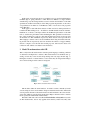
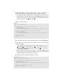
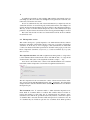
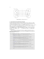
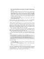
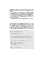
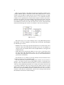
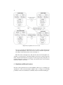
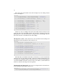
of declarative and imperative constructs. ATL transformations are unidirectional, operating on read-only source models and producing write-only target models (Fig. 1).
During the execution of a transformation, source models may be navigated but changes
are not allowed. Target models cannot be navigated.
Fig. 1. ATL model transformation schema.
ATL modules define the transformations. A module contains a mandatory header
section, an import section, and a number of helpers and transformation rules. The header
section provides the name of the transformation module and declares the source and target models (which are typed by their metamodels). Helpers and rules are the constructs
used to specify the transformation functionality.
Declarative ATL rules can be classified in matched rules and lazy rules. Lazy rules
are like matched rules, but are only applied when called by another rule. They both
3
specify relations between source patterns and target patterns. The source pattern of a
rule specifies a set of source types and an optional guard given as a Boolean expression
in OCL. A source pattern is evaluated to a set of matches in source models. The target
pattern is composed of a set of elements. Each of these elements specifies a target type
from the target metamodel and a set of bindings. A binding refers to a feature of the type
(i.e., an attribute, a reference or an association end) and specifies an expression whose
value is used to initialize the feature. Lazy rules can be called several times using a
collect construct. Unique lazy rules are a special kind of lazy rules that always return
the same target element for a given source element. The target element is retrieved by
navigating the internal traceability links, as in normal rules. Non-unique lazy rules do
not navigate the traceability links, but create new target elements in each execution.
In some cases, complex transformation algorithms may be required, and it may
be difficult to specify them in a declarative way. For this reason ATL provides two
imperative constructs: called rules and action blocks. A called rule is a rule called by
other ones in a procedural style. An action block is a sequence of imperative statements
and can be used instead of, or in combination with, a target pattern in matched or called
rules. The imperative statements in ATL are the usual constructs for attribute assignment
and control flow: conditions and loops.
The ATL Module data type also provides the resolveTemp operation for dealing
with complex transformations. This specific operation makes it possible to refer, from
an ATL rule, to any of the target model elements (including non-default ones) that will
be generated from a given source model element by an ATL matched rule. The signature
of the resolveTemp operation is: resolveTemp(var, target pattern name). The parameter
var corresponds to an ATL variable that contains the source model element from which
the searched target model element is produced. The parameter target pattern name is a
string value that encodes the name of the target pattern element that maps the provided
source model element (contained by var) into the searched target model element. This
operation can be called from the target pattern and imperative sections of any matched
or called rule.
ATL has two execution modes, the normal (default) execution mode and the refining
one.
– In the default execution mode, the ATL developer has to specify, either by matched
or called rules, the way to generate each of the expected target model elements. This
execution mode suits most ATL transformations where source and target metamodels are different.
– The refining execution mode was introduced to ease the programming of refining
transformations between source and target models conforming to the same metamodels. With the refining mode, ATL developers can focus on the ATL code dedicated to the generation of modified target elements. This mode will be further
explained in Section 2.5.
From now on, unless otherwise stated, we will refer to the default execution mode.
In the rest of this section we will introduce the metamodels and models that will be used
throughout the paper, as well as all the ATL transformations that will be later encoded
in Maude for both execution modes.
4
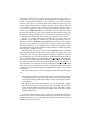
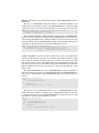
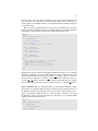
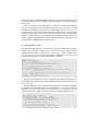
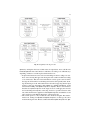
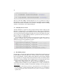
(a) Source metamodel.
(b) Target metamodel.
Fig. 2. Transformation metamodels.
2.1
Metamodels and models
In order to illustrate our proposal let us present here the metamodels that will be used for
our transformations examples. They are the ones used in the example of JavaSouraceto-Table model transformation. This example and many others can be found in [11].
The two metamodels involved in this transformation are shown in Fig. 2.
In the JavaSource metamodel (Fig. 2(a)) we see that Java sources are modeled by a
JavaSource element. This element is composed of ClassDeclarations. Each ClassDeclaration is composed of MethodDefinitions. Both ClassDeclaration and MethodDefinition
inherit from the abstract NamedElement class (which provides a name). A MethodDefinition is composed of MethodInvocations (a call to a method). Each MethodInvocation
is, in turn, associated with one and only one MethodDeclaration (the called method).
The Table metamodel (Fig. 2(b)) shows that Tables are composed of several Rows
that, in turn, are composed of several Cells, each of them having a content.
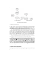
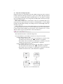
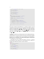
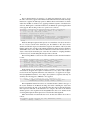
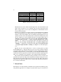
Our input model for all the transformations that will be presented contains a JavaSource with two classes: FirstClass and SecondClass. The former class contains two
methods, fc m1 and fc m2. The first one does not contain any invocation, but the second
one has two of them and both call the first method, fc m1. Regarding the other class, it
also contains two methods, sc m1 and sc m2. The former one has an invocation to the
method fc m1 of the FirstClass. The latter, in turn, has an invocation to the first method
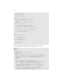
of this class, sc m1. This model is shown in Fig. 3. Its corresponding target model when
the JavaSource2Table transformation shown in Section 2.2 is applied over it is the Table
model shown in Fig. 4.
2.2
ATL declarative transformations
Here we present the transformation needed to get the target model presented in the
previous subsection from the source model. It can be found in [11]. It is composed of
5
Fig. 3. JavaSource input model.
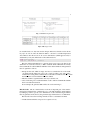
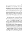
Fig. 4. Table target model.
two matched rules, two lazy rules and two helpers. Please note that the version shown
in [11] is an old one since the function distinct ... foreach is considered deprecated
since ATL 3.0. For this reason, in our version, this function (which appears twice) is
substituted by a lazy rule. The header of the transformation is:
module JavaSource2Table ;
c r e a t e OUT : Table from IN : JavaSource ;
The aim of this transformation is to generate, from a Java source code (that is, the
declaration of several Java classes), a Table document which summarizes how many
times each method is called within the definition of the declared methods. The generated
table is organized as follows:
– Except the first cell, which is empty, the first row contains the list of the methods declared in the input Java source code, sorted according to the “class name.method name” string, where “method name” is the name of a method, and “class name”
the name of the class in which the method is defined.
– The first column is organized in the same way as the first row.
– Cells of following rows contain the number of calls of the in-column method within
the in-row method declaration.
In our example, the generated Table will be the one shown in Fig. 4.
Matched rules. The two matched rules are the most important part of the transformation since matched rules constitute the core of an ATL declarative transformation
by making it possible to specify 1) for which kinds of source elements target elements
must be generated, and 2) the way the generated target elements have to be initialized.
The first rule creates the following elements for the root JavaSource element:
– A Table element which is composed of a sequence of rows;
6
– A Row element, linked to the Table element, which corresponds to the first row of
the Table. This element is composed of the following sequence of elements:
• An empty Cell, linked to the Row element, which is the first cell of the first row.
• One Cell, linked to the Row element, for each MethodDefinition. The content of
the Cell is equal to the “class name.method name” string. Within the sequence,
Cells are ordered according to their content.
Its ATL code is the following:
r u l e Main {
from
s : JavaSource ! JavaSource
to
-- Table is composed of the first row + data rows
t : Table ! Table (
rows <− S e q u e n c e {first_row ,
thisModule . allMethodDefs−>collect ( e | thisModule . resolveTemp ( e , ’row’ ) ) }
),
-- First row is composed of the first column + title columns
first_row : Table ! Row (
cells <− S e q u e n c e {first_col ,
thisModule . allMethodDefs−>collect ( e | thisModule . getContentFirstRow ( e ) ) }
),
-- First column empty
first_col : Table ! Cell (
content <− ’’
)
}
The second matched rule creates the following elements for each MethodDefinition:
– A Row linked to the Table element. This element is composed of the following
sequence of elements:
• A title Cell, linked to the current Row element. Its content is equal to the “classname.method name” string, where “class name” is the name of the class associated with the current MethodDefinition, and “method name” is the name of
the current MethodDefinition.
• One Cell, linked to the current Row element, for each MethodDefinition. The
content of this Cell corresponds to the number of calls of the in-column method
within the definition of the current in-row method.
The ATL representation of this rule in Maude is as follows:
r u l e MethodDefinition {
from
m : JavaSource ! MethodDefinition
to
-- Rows are composed of the first (title) cell + data cells
row : Table ! Row (
cells <− S e q u e n c e {title_cel ,
thisModule . allMethodDefs −> collect ( e | thisModule . getComputeContent ( m , e ) ) }
),
-- Title cell = ’class_name.method_name’
title_cel : Table ! Cell (
content <− m . class . name + ’.’ + m . name
)
}
7
Helpers. Two helpers are used in this transformation, named allMethodDefs and computeContent.
The first one, allMethodDefs, builds the sequence of all method definitions in all
existing classes. The sequence it returns, of type MethodDefinition, is ordered according
1) their class name, and 2) their method name. The code of this helper is the following:
h e l p e r d e f : allMethodDefs : S e q u e n c e ( JavaSource ! MethodDefinition ) =
JavaSource ! MethodDefinition . allInstances ( ) −>
sortedBy ( e | e . class . name + ’_’ + e . name ) ;
The computeContent helper returns the number of calls of an in-column MethodDefinition (provided as a parameter) within the current MethodDefinition. For this purpose, it
selects, among MethodInvocations within the definition, those that have the same class
and method names that the MethodDefinition parameter. The rule then returns the size
of the built set. The representation of this helper in Maude is as follows:
h e l p e r context JavaSource ! MethodDefinition
d e f : computeContent ( col : JavaSource ! MethodDefinition ) : S t r i n g =
self . invocations −> select ( i | i . method . name = col . name and
i . method . class . name = col . class . name )
−>size ( ) ;
“Collect” lazy rules. Lazy rules are like matched rules, but are only applied when
called by another rule. Two lazy rules are used in this transformation. Please note that
both of them are called from matched rules using a collect. It is done this way when
there is the needed to call lazy rules multiple times. We distinguish between these lazy
rules and the ones that are not called with a collect since the internal representation in
Maude is different. For this reason, in Section 2.3, a lazy rule called without a collect
will be shown.
The getContentFirstRow rule receives a MethodDefinition as input and generates a
Cell whose content is the name of the ClassDeclaration that the MethodDefinition belongs to plus ‘.’ plus the name of the MethodDefinition. The code of this lazy rule is as
follows.
l a z y r u l e getContentFirstRow {
from
m : JavaSource ! MethodDefinition
to
c : Table ! Cell (
content <− m . class . name + ’.’ + m . name
)
}
The other lazy rule, getComputeContent, receives two MethodDefinition and generates a Cell whose content is calculated by the computeContent helper. In this case,
it computes the content of the second MethodDefinition according to the first one. The
representation of this lazy rule in Maude is as follows:
l a z y r u l e getComputeContent{
from
m1 : JavaSource ! MethodDefinition ,
m2 : JavaSource ! MethodDefinition
to
c : Table ! Cell (
content <− m1 . computeContent ( m2 ) . toString ( )
)
}
8
2.3
Lazy rules vs Unique lazy rules
Unique lazy rules are a special kind of lazy rules. When a unique lazy rule is executed,
it always returns the same target element for a given source element. The target element
is retrieved by navigating the internal traceability links, in a way similar to standard
rules. Non-unique lazy rules do not navigate the traceability links, and create new target
elements in each execution.
The concept of unique rule is useful when we have non-containment links in our
metamodel. In our target metamodel we only have containment links, so we have slightly
modified our Table metamodel (Fig. 5) by adding a new class called CellType. This way,
Cells have a type now.
In this subsection we present a transformation that uses a (non-unique) lazy rule and
whose target metamodel conforms to the new metamodel. The same transformation
is then executed with an unique lazy rule instead of the non-unique one to see the
difference in the target model. The header of the transformation is:
module JavaSource2TableLazyRule ;
c r e a t e OUT : Table from IN : JavaSource ;
The transformation carries out the following actions:
– For each JavaSource, a new Table is created. It is composed of two Rows.
• The first Row contains two Cells.
∗ The content of the first one is “First row” and the type is created by a lazy
rule which receives the first class of the JavaSource as argument.
∗ The content of the second Cell is ‘5’ and the type is created by a lazy rule
which receives the first class of the JavaSource as argument.
• The second Row contains two Cells too.
∗ The content of the first one is “Second row” and the type is created by a
lazy rule which receives the last class of the JavaSource as argument.
∗ The content of the second Cell is ‘7’ and the type is created by a lazy rule
which receives the last class of the JavaSource as argument.
Fig. 5. New version of Table Metamodel.
9
(a) Transformation with Lazy Rule.
(b) Transformation with Unique
Lazy Rule.
Fig. 6. Models resulting of transformations with Lazy Rule and Unique Lazy Rule.
The mentioned lazy rule receives a ClassDeclaration as input and generates a CellType whose name is the name of the received parameter. The code of this transformation
is:
r u l e Main {
from
s : JavaSource ! JavaSource
to
t : Table ! Table (
rows <− S e q u e n c e {first_row , second_row}
),
first_row : Table ! Row (
cells <− S e q u e n c e {cell_1_1 , cell_1_2}
),
second_row : Table ! Row (
cells <− S e q u e n c e {cell_2_1 , cell_2_2}
),
cell_1_1 : Table ! Cell (
content <− ’First_row’ ,
type <− thisModule . GetType ( s . classes −>
),
cell_1_2 : Table ! Cell (
content <− ’5’ ,
type <− thisModule . GetType ( s . classes −>
) , cell_2_1 : Table ! Cell (
content <− ’Second_row’ ,
type <− thisModule . GetType ( s . classes −>
),
cell_2_2 : Table ! Cell (
content <− ’7’ ,
type <− thisModule . GetType ( s . classes −>
)
}
l a z y r u l e GetType {
from
cd : JavaSource ! ClassDeclaration
to
c : Table ! CellType (
name <− cd . name
)
}
first ( ) )
first ( ) )
last ( ) )
last ( ) )
10
A graphical representation of the resulting Table with this transformation may be
seen in Fig. 6(a). We can see that a new CellType has been generated for each Cell, even
if more that one have the same name.
Now, if we substitute the lazy rule of the transformation by a unique lazy rule, the
obtained model is the one shown in Fig. 6(b). In this transformation, new CellTypes are
created only the first time the unique lazy rule is called (for the same input parameter).
This way, for the second time that the unique lazy rule is called with the same input
parameter, only the reference from the Cell to the already generated CellType is created.
The result of the execution of these two transformations will be shown as a Maude
model in Section 6.1.
2.4
The imperative section
ATL enables developers to specify imperative code within dedicated blocks, either in
matched or called rules. An imperative block is composed of a sequence of imperative
statements. As in the Java C or C++ languages, each statement must be ended with
a semicolon character. The ATL representation described in this paper provides four
kinds of imperative statements: assignments (=), conditional branches (if), loops (for)
and called rules.
The assignment statement. The ATL assignment statement permits to assign values
to either attributes that are defined in the context of the ATL module, or to target model
element features. The syntax of the assignment statement is: target < − exp;.
Let us show a rule which creates a Cell for each ClassDeclaration. It is a matched
rule which contains an imperative section with an assignment statement in it:
r u l e Main {
from
cd : JavaSource ! ClassDeclaration
to
c : Table ! Cell (
content <− cd . name
)
do{
c . content <− c . content + ’_assignment’ ;
}
}
The rule’s imperative block concatenates the content of the Cell created in the declarative section from the ClassDeclaration instance with “ assignment”. Note that in this
example the Cell’s content is initialized in the declarative part and then it is modified in
the imperative part.
The if statement. The “if” statement enables to define alternative imperative treatments. Each “if” statement defines a condition. This condition must be an OCL expression that returns a boolean value. An “if” statement must also include a “then”
statements section. This block, specified between curly brackets, contains the sequence
of statements that is executed when the conditional expression is evaluated to true. An
“if” statement may also include an optional “else” statements block. When specified,
11
this block has to follow the “then” statements section. It is introduced by the keyword
else, and must be also defined between curly brackets. This section contains the optional sequence of statements that has to be executed when the conditional expression
is evaluated to false.
Here we present a matched rule that is composed of a declarative part and an imperative part with assignments and an “if” statement. The rule creates in its declarative
part a Table for each JavaSource. This Table contains a Row and two Cells:
r u l e Main {
from
s : JavaSource ! JavaSource
to
c : Table ! Table (
rows <− S e q u e n c e {row}
),
row : Table ! Row (
cells <− S e q u e n c e {cell1 , cell2 , cell3}
),
cell1 : Table ! Cell (
content <− ’FirstCell’
),
cell2 : Table ! Cell (
content <− ’SecondCell’
),
cell3 : Table ! Cell (
content <− ’ThirdCell’
)
do{
cell1 . content <− cell1 . content + ’_if_condition’ ;
if ( row . cells −> size ( ) = 3 ) {
cell2 . content <− ’Condition_satisfied’ ;
}else{
cell2 . content <− ’Condition_not_satisfied’ ;
}
}
}
The imperative section contains an assignment statement followed by an “if” statement
which also contains an “else” section. This imperative section concatenates the content
of the first Cell created in the declarative part with “ if condition”. The “if” section sets
the name of the second Cell to “Condition satisfied” if the Row contains three Cells or to
“Condition not- satisfied” otherwise. Since the Table contains three Cells as specified
in the declarative part, the name of the second Cell will be set to “Condition satisfied”.
The for statement. The “for” statement enables to define iterative imperative computations. The “for” statement defines an iteration variable (iterator) that will iterate over
the different elements of the reference collection. For each of these elements, the sequence of statements contained by the “for” statement will be executed. Let us extend
the imperative section of the rule shown before to introduce a “for” statement which
contains some imperative instructions:
r u l e Main {
from
s : JavaSource ! JavaSource
to
c : Table ! Table (
rows <− S e q u e n c e {row}
),
row : Table ! Row (
12
cells <− S e q u e n c e {cell1 , cell2 , cell3}
),
cell1 : Table ! Cell (
content <− ’FirstCell’
),
cell2 : Table ! Cell (
content <− ’SecondCell’
),
cell3 : Table ! Cell (
content <− ’ThirdCell’
)
do{
cell1 . content <− cell1 . content + ’_assignment’ ;
if ( row . cells −> size ( ) = 3 ) {
cell2 . content <− ’Condition_satisfied’ ;
}else{
cell2 . content <− ’Condition_not_satisfied’ ;
}
for ( i in row . cells ) {
i . content <− i . content + ’_assign_for’ ;
if ( i . content = ’ThirdCell_assign_for’ ) {
i . content <− i . content + ’_if_for_satisfied’ ;
}else{
i . content <− i . content + ’_if_for_not_satisfied’ ;
}
i . content <− i . content + ’_after_if_for’ ;
}
}
}
The sequence of instructions added within the “for” statement are applied to every Cell
of the Row created by the rule. First of all, an assignment is made, where the content of
each Cell is concatenated with “ assign For”. After that, an “if” section is introduced.
This section concatenates the content of each Cell with “ if for satisfied” if the content
of the Cell was ‘ThirdCell assign for” or with “ if for not satisfied” if it was not. Finally, another assignment is applied, where the contents of the Cells are concatenated
with “ after if for”.
Called Rules. Called rules provide ATL developers with convenient imperative programming facilities. In some way, called rules can be seen as a particular type of helpers
since they have to be explicitly called to be executed and they can accept parameters.
However, as opposed to helpers, called rules can generate target model elements as
matched rules do. A called rule has to be called from an imperative code block, either
from a matched rule or another called rule.
The example below shows a matched rule which has a reference to a called rule
in its imperative part. The declarative part of the matched rule creates a Table from a
JavaSource with a Row and a Cell whose content is “FirstCell”.
r u l e Main {
from
s : JavaSource ! JavaSource
to
c : Table ! Table (
rows <− S e q u e n c e {row}
),
row : Table ! Row (
cells <− S e q u e n c e {cell}
),
cell : Table ! Cell (
content <− ’FirstCell’
13
)
do{
thisModule . NewTable ( ’NewTable’ ) ;
}
}
-- Called rule:
r u l e NewTable ( s : S t r i n g ) {
to
c : Table ! Table (
rows <− S e q u e n c e {row}
),
row : Table ! Row (
cells <− S e q u e n c e {cell}
),
cell : Table ! Cell (
content <− s
)
}
As we can see, the matched rule is calling the NewTable called rule from its imperative
part passing a String as argument. This called rule creates a new Table with a Row and
a Cell whose content is the String passed as argument.
2.5
ATL Refining Mode
Apart from the ATL execution mode considered in the transformations shown so far,
ATL provides developers with the refining mode, so that they can focus on the ATL
code dedicated to the generation of modified target elements.
In the ATL version of 2004, the copying was performed implicitly only for contained elements of copied elements and it was mandatory to specify all bindings. The
effort of copying some elements of a transformation, while modifying others, was reduced in the next version of the ATL language in 2006, which introduced in-place refining mode. In this mode every element stays unchanged if it is not explicitly matched
by a transformation rule.
As explained in [12], the refining mode execution semantics follow three phases:
– Module initialization phase. In this phase, the attributes defined in the context of
the transformation module are initialized.
– Source model elements matching phase. Here, the ATL engine only evaluates the
matching conditions of the explicitly specified matched rules. This implies that,
at this stage, the only target model elements that are allocated are those that are
generated by these explicit transformations rules.
– Initialization phase of the target model elements. As in the normal execution mode,
this phase has to deal with the initialization of the explicitly generated target model
elements. Apart from this, it also deals now with the allocation and the initialization
of the target model elements that are implicitly generated. For this purpose, each
time an already allocated target model element is initialized with a reference to
a non-allocated model element, the ATL engine allocates and initializes this new
target model element. If the newly created model element also refers to another
non-allocated model element, this process is repeated recursively.
14
An application of the refining mode: High-Order Transformations. In ModelDriven Engineering, High-OrderTransformations (HOTs) [21] are model transformations that analyze, produce or manipulate other model transformations. Writing HOTs
is generally considered a time-consuming and error-prone task, and often results in verbose code.
In [20], they present, among others, a proposal to facilitate the definition of HOTs in
ATL based on the in-place refining mode. There are HOTs that do not present a general
semantics of refinement, and they simply need to copy a set of elements from an input
to an output. In these cases a fine-graned refining mode could be beneficial, allowing
the user to choose exactly the subset of the input model that is subject to refinement.
Tisi et al. [20] propose refining rules to give the developer the possibility to specify with
minimal effort that a single element has to be copied to the output model, together with
all its contained and associated elements.
The following piece of code is an excerpt from the MergeHOT transformation that
creates a new transformation by the simple union of transformation rules given in input.
r u l e matchedRule {
from
lr : ATL ! MatchedRule (
lr . isLeft or lr . isRight
)
to
m : ATL ! MatchedRule (
name <− lr . fromLeftOrRight + ’_’ + lr . name ,
children <− lr . children ,
superRule <− lr . superRule ,
isAbstract <− lr . isAbstract ,
isRefining <− lr . isRefining ,
inPattern <− lr . inPattern ,
outPattern <− lr . outPattern
)
}
r u l e inPattern {
from
lr : ATL ! InPattern (
lr . isLeft or lr . isRight
)
to
m : ATL ! InPattern (
elements <− lr . elements
)
}
. . . [ 1 0 0 lines ]
It is a solution in normal execution mode, where the developer is forced to include a
long list of copying rules for all the elements of the two models to merge (e.g., Binding,
NavigationOrAttributeCallExp, VariableExp). Refining rules allow the substitution of
all this code (more than 100 LOCs) with this excerpt:
r u l e matchedRule {
from
lr : ATL ! MatchedRule (
lr . isLeft or lr . isRight
)
to
m : ATL ! MatchedRule (
name <− lr . fromLeftOrRight + ’_’ + lr . name ,
)
}
15
The refining rule states that the matching rule has to be copied to the output model
with a different name, and implicitly triggers the recursive copy of all the elements
contained in this matching rule, making the other HOT rules superfluous.
Similarly to the previous proposal, refining rules could provide a noticeable gain in
HOT conciseness, but also a general impact on ATL productivity outside HOT development.
Transformation developed using the ATL refining mode. In this subsection we
present and describe the Public2Private transformation which can be found in [11].
This transformation makes all public attributes of a UML model private using refining
mode. Getters and setters are also created appropriately. The representation in ATL of
the transformation is the following:
module Public2Private ;
c r e a t e OUT : UML refining IN : UML ;
h e l p e r context S t r i n g d e f : toU1Case : S t r i n g =
self . substring ( 1 , 1 ) . toUpper ( ) +
self . substring ( 2 , self . size ( ) ) ;
r u l e Property {
from
publicAttribute : UML ! Property (
publicAttribute . visibility = #public
)
to
privateAttribute : UML ! Property (
visibility <− #private
),
getter : UML ! Operation (
name <− ’get’+publicAttribute . name . toU1Case ,
class <− publicAttribute . refImmediateComposite ( ) ,
type <− publicAttribute . type
),
setter : UML ! Operation (
name <− ’set’+publicAttribute . name . toU1Case ,
class <− publicAttribute . refImmediateComposite ( ) ,
ownedParameter <− setterParam
),
setterParam : UML ! Parameter (
name <− publicAttribute . name ,
type <− publicAttribute . type
)
}
This is what the transformation does:
– Objects of type Property which have their visibility attribute set to #public in the
source model are modified so that in the target model the attribute is set to #private
and their other attributes are unmodified.
– Three new objects are created in the target model from the Property object: one
getter operation, one setter operation, and the parameter for the setter operation.
– All the objects that are not properties with the visibility attribute set to #public remain
unchanged in the target model.
16
3
Rewriting Logic and Maude
Maude [6] is a high-level language and a high-performance interpreter in the OBJ algebraic specification family that supports membership equational logic [5] and rewriting
logic [14] specification and programming of systems. Thus, Maude integrates an equational style of functional programming with rewriting logic computation. Because of
its efficient rewriting engine, able to execute more than 3 million rewriting steps per
second on standard PCs, and because of its metalanguage capabilities, Maude turns out
to be an excellent tool to create executable environments for various logics, models
of computation, theorem provers, or even programming languages. We informally describe in this section those Maude’s features necessary for understanding the paper; the
interested reader is referred to [6] for more details.
Rewriting logic is a logic of change that can naturally deal with state and with
highly nondeterministic concurrent computations. A distributed system is axiomatized
in rewriting logic by a rewrite theory R = (Σ, E , R), where (Σ, E ) is an equational
theory describing its set of states as the algebraic data type TΣ/E associated to the
initial algebra (Σ, E ), and R is a collection of rewrite rules. Maude’s underlying equational logic is membership equational logic [5], a Horn logic whose atomic sentences
are equalities t = t 0 and membership assertions of the form t : S , stating that a term t
has sort S . Such a logic extends order-sorted equational logic, and supports sorts, subsort relations, subsort overloading of operators, and definition of partial functions with
equationally defined domains.
Rewrite rules, which are written crl [l ] : t => t 0 if Cond , with l the rule label, t
and t 0 terms, and Cond a condition, describe the local, concurrent transitions that are
possible in the system, i.e., when a part of the system state fits the pattern t, then it can
be replaced by the corresponding instantiation of t 0 . The guard Cond acts as a blocking
precondition, in the sense that a conditional rule can be fired only if its condition holds.
The form of conditions is EqCond1 /\ ... /\ EqCondn where each of the EqCondi
is either an ordinary equation t = t 0 , a matching equation t := t 0 , a sort constraint t : s , or
a term t of sort Bool, abbreviating the equation t = true. In the execution of a matching
equation t := t 0 , the variables of the term t , which may not appear in the left hand side
of the corresponding conditional equation, become instantiated by matching the term t
against the canonical form of the bounded subject term t 0 .
For instance, the following Maude module, ACCOUNT, specifies a class Account
with an attribute balance of sort integer (Int), and other class Withdraw (that models the
action of withdrawing) with an object identifier (of sort Oid) and an integer as attributes,
and a rule describing the behavior of the objects belonging to these classes. The rule
debit specifies a local transition of the system when there is an object A of class Account
and a Withdraw object requesting to withdraw an amount smaller or equal than the
balance of A; as a result of the application of such a rule, the object representing the
action is consumed, and the balance of the account is modified.
( omod ACCOUNT i s
p r o t e c t i n g INT .
c l a s s Account | balance : Int .
c l a s s Withdraw | acc : Oid , amount : Int .
v a r s A W : Oid .
v a r s M Bal : Int .
17
c r l [ debit ] :
< W : Withdraw | acc : A , amount : M >
< A : Account | balance : Bal >
=> < A : Account | balance : Bal − M >
i f M <= Bal .
endom )
4
ATL Default Execution Mode in Maude
To give a formal semantics to ATL using rewriting logic, we provide a representation
of ATL constructs and behavior in Maude. We start by defining how the models and
metamodels handled by ATL can be encoded in Maude, and then provide the semantics
of matched rules, lazy rules, unique lazy rules, helpers and imperative sections (assignment statements, if statements, loops and called rules). One of the benefits of such an
encoding is that it is systematic and can be automated, something we plan to implement
using ATL transformations (between the ATL and Maude metamodels). The interested
reader could find all the examples shown here in [22].
4.1
Characterizing Model Transformations
In our view, a model transformation is just an algorithmic specification (let it be declarative or operational) associated to a relation R ⊆ MM × MN defined between two
metamodels which allows to obtain a target model N conforming to MN from a source
model M that conforms to metamodel MM [19].
The idea supporting our proposal considers that model transformations comprise
two different aspects: structure and behavior. The former aspect defines the structural
relation R that should hold between source and target models, whilst the latter describes
how the specific source model elements are transformed into target model elements.
This separation allows differentiating between the relation that the model transformation ensures, from the algorithm it actually uses to compute the target model from the
source model.
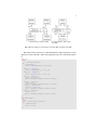
Thus, to represent the structural aspects of a transformation we will use three models: the source model M , the target model N that the transformation builds, and the
relation R(M , N ) between the two. R(M , N ) is also called the trace model, that specifies how the elements of M and N are consistently related by R. Please note that each
element ri of R(M , N ) = {r1 , ..., rk } ⊆ P(M ) × P(N ) relates a set of elements of M
with a set of elements of N (see Fig. 7).
Note that this approach works not only for providing structural semantics to ATL,
but to any model transformation language. In fact, the set R(M , N ) = {r1 , ..., rk } is
nothing but the set of all trace instances of the transformation.
The behavioral aspects of an ATL transformation (i.e., how the transformation progressively builds the target model elements from the source model, and the traces between them) is defined using the different kinds of rules (matched, lazy, unique lazy);
their possible combinations and direct invocation from other rules, and the final imperative algorithms that can be invoked after each rule.
The rest of this section describes how both the structural and behavioral aspects of
ATL transformations can be encoded in Maude.
18
Fig. 7. Elements of a relation R(M , N ).
4.2
Encoding Models and Metamodels in Maude
We will follow the representation of models and metamodels introduced in [16], which
is inspired in the Maude representation of object-oriented systems mentioned above. We
represent models in Maude as structures of sort @Model of the form mm{obj1 obj2 ... objN },
where mm is the name of the metamodel and obji are the objects that constitute the
model. An object is a record-like structure of the form < o : c | a1 : v1 , ..., an : vn >
(of sort @Object), where o is the object identifier (of sort Oid), c is the class the object
belongs to (of sort @Class), and ai : vi are attribute-value pairs (of sort @StructuralFeatureInstance).
Given the appropriate definitions for all classes, attributes and references in its corresponding metamodel (as we shall see below), the following Maude term describes the
input model shown in Section 2.
@javasourcemm@ {
< ’s : JavaSource@javasourcemm | classes@JavaSource@javasourcemm :
Sequence [ ’c1 ; ’c2 ] >
< ’c1 : ClassDeclaration@javasourcemm | name@NamedElement@javasourcemm :
"FirstClass" # methods@ClassDeclaration@javasourcemm :
Sequence [ ’m1 ; ’m2 ] >
< ’m1 : MethodDefinition@javasourcemm | name@NamedElement@javasourcemm :
"fc_m1" # invocations@MethodDefinition@javasourcemm : null #
class@MethodDefinition@javasourcemm : ’c1 >
< ’m2 : MethodDefinition@javasourcemm | name@NamedElement@javasourcemm :
"fc_m2" # invocations@MethodDefinition@javasourcemm :
Sequence [ ’i1 ; ’i1 ] # class@MethodDefinition@javasourcemm : ’c1 >
< ’i1 : MethodInvocation@javasourcemm | method@MethodInvocation@javasourcemm :
’m1 >
< ’c2 : ClassDeclaration@javasourcemm | name@NamedElement@javasourcemm :
"SecondClass" # methods@ClassDeclaration@javasourcemm :
Sequence [ ’m3 ; ’m4 ] >
< ’m3 : MethodDefinition@javasourcemm | name@NamedElement@javasourcemm :
"sc_m1" # invocations@MethodDefinition@javasourcemm : ’i2 #
class@MethodDefinition@javasourcemm : ’c2 >
< ’i2 : MethodInvocation@javasourcemm | method@MethodInvocation@javasourcemm :
’m1 >
< ’m4 : MethodDefinition@javasourcemm | name@NamedElement@javasourcemm :
"sc_m2" # invocations@MethodDefinition@javasourcemm : ’i3 #
class@MethodDefinition@javasourcemm : ’c2 >
< ’i3 : MethodInvocation@javasourcemm | method@MethodInvocation@javasourcemm :
’m3 >
}
19
Note that quoted identifiers are used as object identifiers; references are encoded as
object attributes by means of object identifiers; symbol # is used as a separator between
attributes; and OCL collections (Set, OrderedSet, Sequence, and Bag) are supported by
means of mOdCL [17].
Metamodels are encoded using a sort for every metamodel element: sort @Class
for classes, sort @Attribute for attributes, sort @Reference for references, etc. Thus, a
metamodel is represented by declaring a constant of the corresponding sort for each
metamodel element. More precisely, each class is represented by a constant of a sort
named after the class. This sort, which will be declared as subsort of sort @Class, is defined to support class inheritance through Maude’s order-sorted type structure. The following Maude specification describes a fragment of the JavaSource metamodel shown
in Fig. 2(a).
mod @JAVASOURCEMM@ i s
p r o t e c t i n g @ECORE@ .
op @javasourcemm@ : −> @Metamodel .
op javasourcemm : −> @Package .
s o r t ClassDeclaration@javasourcemm .
s u b s o r t s ClassDeclaration@javasourcemm < NamedElement@javasourcemm .
op ClassDeclaration@javasourcemm : −> ClassDeclaration@javasourcemm .
op methods@ClassDeclaration@javasourcemm : −> @Reference
...
s o r t MethodDefinition@javasourcemm .
s u b s o r t s MethodDefinition@javasourcemm < NamedElement@javasourcemm .
op MethodDefinition@javasourcemm : −> MethodDefinition@javasourcemm .
op invocations@MethodDefinition@javasourcemm : −> @Reference
...
endm
Other properties of metamodel elements, such as whether a class is abstract or not, the
opposite of a reference (to represent bidirectional associations), or attributes and reference types, are expressed by means of Maude equations defined over the constant that
represents the corresponding metamodel element. Classes, attributes and references are
qualified with their containers’ names, so that classes with the same name belonging
to different packages, as well as attributes and references of different classes, are distinguished. These qualifications are omitted here to improve readability. See [16] for
further details.
4.3
Declarative transformation written in Maude
Here we represent in Maude the ATL transformation which was explained in Section 2.2. This transformation is composed of matched rules, lazy rules called with a
collect, and helpers, so we are going to explain in the following subsections how all
these concepts are translated into Maude.
Matched rules in Maude. Each ATL matched rule is represented by a Maude rewrite
rule that describes how the target model elements are created from the source model
elements identified in the left-hand side of the rule (that represents the “to” pattern of
the ATL rule). The general form of such rewrite rules is the following:
20
c r l [ rulename ] :
Sequence [
( @SourceMm@ { . . . OBJSET@ }) ;
( @TraceMm@ { . . . OBJSETT@ }) ;
( @TargetMm@ { OBJSETTT@ }) ]
=>
Sequence [
( @SourceMm@ { . . . OBJSET@ }) ;
( @TraceMm@ { . . . OBJSETT@}) ;
( @TargetMm@ { . . . OBJSETTT@ }) ]
if . . .
/ \ not alreadyExecuted ( . . . , "rulename" , @TraceMm@ { OBJSETT@ }) .
The two sides of the Maude rule contains the three models that capture the state
of the transformation (see 4.1): the source, the trace and the target models. The rule
specifies how the state of the ATL model transformation changes as result of such rule.
The triggering of Maude and ATL rules is similar: a rule is triggered if the pattern
specified by the rule is found, and the guard condition holds. In addition to the specific
rule conditions, in the Maude representation we also check (alreadyExecuted) that the
same ATL rule has not been triggered with the same elements.
An additional Maude rule, called Init, starts the transformation. It creates the initial
state of the model transformation, and initializes the target and trace models:
r l [ Init ] :
Sequence [ ( @JavaSourceMM@ { OBJSET@ }) ]
=> Sequence [
( @JavaSourceMM@ { OBJSET@ }) ;
( @TraceMm@ { < ’CNT : Counter@CounterMm | value@Counter@CounterMm : 1 > }) ;
( @TableMM@ { none }) ] .
The traces stored in the trace model are also objects, of class Trace@TraceMm,
whose attributes are: two sequences (srcEl@TraceMm and trgEl@TraceMm) with the
sets of identifiers of the elements of the source and target models related by the trace;
the rule name (rlName@TraceMm); and a reference to the source and target metamodels:
srcMdl@TraceMm and trgMdl@TraceMm.
The trace model also contains a special object, of class Counter@CounterMm, whose
integer attribute is used as a counter for assigning fresh identifiers to the newly created
elements and traces.
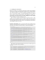
In the following we will present how to translate the two matched rules presented
in Section 2.2 in Maude. We also use some auxiliary functions that will also be shown.
We start by showing the header of the whole Maude file containing the two matched
rules, two helpers and two lazy rules, which is:
mod @JAVASOURCE2TABLE@ i s
protecting
protecting
protecting
protecting
@JAVASOURCEMM@ .
@TRACEMMN@ .
@TABLEMM@ .
@FUNCTIONS4ATL@ .
v a r s M1@ M2@ S@ T@ FR@ FC@ R@ FR@ M@ SELF@ COL@ CNT@ TR@ TR2@ : Oid .
op ITER : −> Vid .
var SFS : Set{@StructuralFeatureInstance} .
var OBJSET@ OBJSETT@ OBJSETTT@ : Set{@Object} .
var VALUE@CNT@ OBJS@CREATED@ I@ : Int .
var JAVASOURCEMODEL@ TRACEMODEL@ Java : @Model .
var LO : ListOrd .
21
Here, @JAVASOURCEMM@ is the source metamodel (JavaSource metamodel) of the
transformation, @TABLEMM@ is the target metamodel (Table metamodel), @TRACEMM@
is the additional metamodel for keeping all the traces of the transformation, and FUNCTIONS4ATL contains some additional functions that will be shown later. The rest are
variables that will be used throughout the whole transformation.
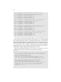
Let us start presenting the second rule, MethodDefinition:
c r l [ MethodDefinition ] :
Sequence [
( @JavaSourceMM@ {
< M@ : MethodDefinition@JavaSourceMM | SFS >
OBJSET@ }) ;
( @TraceMm@ {
< CNT@ : Counter@CounterMm | value@Counter@CounterMm : VALUE@CNT@ >
OBJSETT@ }) ;
( @TableMM@ { OBJSETTT@ })
]
=>
Sequence [
( @JavaSourceMM@ {
< M@ : MethodDefinition@JavaSourceMM | SFS >
OBJSET@ }) ;
( @TraceMm@ {
< CNT@ : Counter@CounterMm | value@Counter@CounterMm : VALUE@CNT@ + I@ + 4 >
--- Trace corresponding to the execution of this matched rule:
< TR@ : Trace@TraceMm | srcEl@TraceMm : Sequence [ M@ ] # trgEl@TraceMm :
Sequence [ R@ ; FC@ ] # rlName@TraceMm : "MethodDefinition" # srcMdl@TraceMm :
"JavaSource" # trgMdl@TraceMm : "Table" >
--- Trace corresponding to the execution of the lazy rule
--- ’computeContentCollect’:
< TR2@ : Trace@TraceMm | srcEl@TraceMm : << Sequence [ M@ ] −>
union ( allMethodDefs ( JAVASOURCEMODEL@ ) ) >> # trgEl@TraceMm : <<
getOidsCollect ( allMethodDefs ( JAVASOURCEMODEL@ ) , VALUE@CNT@ + 1 , 1 ) −>
asSequence ( ) >> # rlName@TraceMm :
"MethodDefinition_computeContentCollect" # srcMdl@TraceMm :
"JavaSource" # trgMdl@TraceMm : "Table" >
OBJSETT@}) ;
( @TableMM@ {
< R@ : Row@tablemm | cells@Row@TableMM : << Sequence [ FC@ ] −>
union ( getOidsCollect ( allMethodDefs ( JAVASOURCEMODEL@ ) ,
VALUE@CNT@ + 1 , 1 ) ) >> >
computeContentCollect ( M@ , allMethodDefs ( JAVASOURCEMODEL@ ) , JAVASOURCEMODEL@ ,
VALUE@CNT@ + 1 )
< FC@ : Cell@tablemm | content@Cell@TableMM :
<< M@ . class@MethodDefinition@javasourcemm .
name@NamedElement@JavaSourceMM + "." + M@ .
name@NamedElement@JavaSourceMM ; JAVASOURCEMODEL@ >> >
OBJSETTT@ })
]
if
JAVASOURCEMODEL@ : = ( @JavaSourceMM@ {
< M@ : MethodDefinition@JavaSourceMM | SFS >
OBJSET@ }) / \
I@ : = 1 + << allMethodDefs ( JAVASOURCEMODEL@ ) −> size ( ) ;
JAVASOURCEMODEL@ >> / \
TR@ : = newId ( VALUE@CNT@ + I@ + 1 ) / \ R@ : = newId ( VALUE@CNT@ + I@ + 2 ) / \
FC@ : = newId ( VALUE@CNT@ + I@ + 3 ) / \ TR2@ : = newId ( VALUE@CNT@ + I@ + 4 ) / \
not alreadyExecuted ( Sequence [ M@ ] , "MethodDefinition" , @TraceMm@ { OBJSETT@ })
.
This rule is applied over MethodDefinition instances. This is specified by requiring
that in the JavaSource model in the left hand side of the rule there must be an instance
of type MethodDefinition@JavaSourceMM. The trace model has to contain an element
22
of type Counter and it does not matter what the Table model contains in the left hand
side for this rule to be triggered.
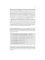
The JavaSource model does not change in the right hand side of the rule, but the
other two models need to change. In this way, a new Row (R@) is added to the Table
model. The cells reference of this new Row is composed of a new Cell (FC@), which
acts as the first Cell of the Row, created by this rule and a set of Cells created by a lazy
rule called with a collect. This lazy rule is explained in Section 4.3. One of its arguments
is a helper, named allMethodDefs, that is explained in Section 4.3.
We allow the evaluation of OCL expressions using mOdCL [17] by enclosing them
in double angle brackets (<< ... >>). Thus, the sentence << Sequence [ TC@ ] − >
union (getOidsCollect(allMethodDefs(JAVASOURCEMODEL@), VALUE@CNT@ + 1,
1)) >> concatenates two sequences with the Cells mentioned, where JAVASOURCEMODEL@ represents the JavaSource model as specified in the first condition. The Cell
created by this rule, which is the first one of the Row, is also added as a new object. Its
content is set by an OCL expression which concatenates the name of the ClassDeclaration of the MethodDefinition plus ‘.’ plus the name of the MethodDefinition (<< M@ .
class@MethodDefinition@javasourcemm . name@NamedElement@JavaSourceMM +
”.” + M@ . name@NamedElement@JavaSourceMM ; JAVASOURCEMODEL@ >>).
Two new traces are added by this rule. The first one is needed to record the execution
of this matched rule and the second one is needed to record the execution of the lazy
rule. It will be explained in Section 4.3. The first trace, TR@, has a sequence with the
MethodDefinition as source element and a sequence with the Row and Cell created by
this matched rule as target element. The value of the counter is increased in the right
hand side with the number of elements created, since it needs to be used in the following
rule that will be applied. This counter is used in the conditions, by the newId function,
to give fresh identifiers to the newly created elements (the trace, Cell and Row in this
case) with the function newId. The object I@, which is an integer, is given a value which
depends on the number of objects created by the lazy rule and is used when giving new
identifiers to the elements created in the matched rule. In this way, the elements created
in the lazy rule and in the matched rule are always different. The newId function is
found in the FUNCTIONS4ATL module:
op newId : Int −> Qid .
eq newId ( I : Int ) = oid ( I : Int ) .
Here, Qid is the type that represents the identifiers of objects. This function uses another
one called oid:
op oid : Int −> Qid .
eq oid ( I : Int ) = qid ( string ( I : Int , 1 0 ) ) .
The Qid created by this function is a string with contains the caracter ’ concatenated
with the Integer passed as argument.
The last condition of the rule, that uses the function alreadyExecuted, ensures that
this rule will not be applied again with the same MethodDefinition. This function is also
found in the FUNCTIONS4ATL module and is the next:
op alreadyExecuted : Sequence String @Model −> Bool .
eq alreadyExecuted ( SEQ , NAME , @TraceMm@ { < TR@ : Trace@TraceMm |
srcEl@TraceMm : SEQ # rlName@TraceMm : NAME # SFS > OBJSET }) = true .
eq alreadyExecuted ( SEQ , NAME , @TraceMm@ { OBJSET }) = false [ owise ] .
23
The function returns true if there exists a trace in the trace model whose source element is the sequence passed as argument and the name passed is the name of the rule.
Otherwise, it returns false.
The other matched rule, named Main, is represented in Maude as follows:
c r l [ Main ] :
Sequence [
( @JavasourceMM@ {
< S@ : JavaSource@JavasourceMM | SFS >
OBJSET@ }) ;
( @TraceMm@ {
< CNT@ : Counter@CounterMm | value@Counter@CounterMm : VALUE@CNT@ >
OBJSETT@ }) ;
( @TableMM@ { OBJSETTT@ })
]
=>
Sequence [
( @JavasourceMM@ {
< S@ : JavaSource@JavasourceMM | SFS >
OBJSET@ }) ;
( @TraceMm@ {
< CNT@ : Counter@CounterMm | value@Counter@CounterMm : VALUE@CNT@ + I@ + 4 >
--- Trace corresponding to the execution of this matched rule:
< TR@ : Trace@TraceMm | srcEl@TraceMm : Sequence [ S@ ] # :
Sequence [ T@ ; FR@ ; FC@ ] # rlName@TraceMm : "Main" # srcMdl@TraceMm :
"JavaSource" # trgMdl@TraceMm : "Table" >
--- Trace corresponding to the execution of the lazy rule
--- ’getContentFirstRowCollect’:
< TR2@ : Trace@TraceMm | srcEl@TraceMm : << allMethodDefs ( JAVASOURCEMODEL@ )
−> asSequence ( ) >> # trgEl@TraceMm : <<
getOidsCollect ( allMethodDefs ( JAVASOURCEMODEL@ ) , VALUE@CNT@ + 1 , 1 ) −>
asSequence ( ) >> # rlName@TraceMm : "Main_getContentFirstRowCollect" #
srcMdl@TraceMm : "JavaSource" # trgMdl@TraceMm : "Table" >
OBJSETT@}) ;
( @TableMM@ {
< T@ : Table@TableMM | rows@Table@TableMM : << Sequence [ FR@ ] −>
union ( resolveTempCollect ( allMethodDefs ( JAVASOURCEMODEL@ ) , 1 ,
@TraceMm@ {OBJSETT@}) ) >> >
< FR@ : Row@tablemm | cells@Row@tablemm : << Sequence [ FC@ ] −> union
( getOidsCollect ( allMethodDefs ( JAVASOURCEMODEL@ ) , VALUE@CNT@ + 1 , 1 ) ) >> >
getContentFirstRowCollect ( allMethodDefs ( JAVASOURCEMODEL@ ) , JAVASOURCEMODEL@ ,
VALUE@CNT@ + 1 )
< FC@ : Cell@TableMM | content@Cell@TableMM : " " >
OBJSETTT@ })
]
if
JAVASOURCEMODEL@ : = ( @JavasourceMM@ {
< S@ : JavaSource@JavasourceMM | SFS >
OBJSET@ }) / \
I@ : = 1 + << allMethodDefs ( JAVASOURCEMODEL@ ) −> size ( ) ;
JAVASOURCEMODEL@ >> / \
TR@ : = newId ( VALUE@CNT@ ) / \ T@ : = newId ( VALUE@CNT@ + 1 ) / \
FR@ : = newId ( VALUE@CNT@ + 2 ) / \ FC@ : = newId ( VALUE@CNT@ + 3 ) / \
TR2@ : = newId ( VALUE@CNT@ + 4 ) / \
<< allMethodDefs ( JAVASOURCEMODEL@ ) −> size ( ) ; JAVASOURCEMODEL@ >> ==
<< resolveTempCollect ( allMethodDefs ( JAVASOURCEMODEL@ ) , 1 ,
@TraceMm@ {OBJSETT@}) −> size ( ) ; JAVASOURCEMODEL@ >> / \
not alreadyExecuted ( Sequence [ S@ ] , "Main" , @TraceMm@ { OBJSETT@ })
.
This rule is applied over JavaSource instances. This is specified by requiring that
in the JavaSource model in the left hand side of the rule there must be an instance of
type JavaSource@JavaSourceMM . As in the other rule, the trace model has to contain
an element of type Counter and it does not matter what the Table model contains in the
left hand side for this rule to be triggered.
24
The JavaSource model does not change in the right hand side of the rule, but the
other two models need to change. In this way, a new Table (T@) is added to the Table
model. The rows reference of this Table is composed of a new Row (@FR), which acts
as the first Row, and a set of Rows which are retrieved my means of the resolveTemp
function called with a collect. This function is explained in Section 4.3. As for the
Row created by this rule, FR@, its cells reference is initialized with a new Cell (FC@)
created in this rule and a set of Cells created by a lazy rule called with a collect. This
lazy rule is explained in Section 4.3. Both the lazy rule and the resolveTemp function in
his rule have an argument which is a helper, named allMethodDefs, that is explained in
Section 4.3.
As in the other matched rule, two traces are added by this one, one due to the
execution of this matched rule and the other one, explained in Section 4.3, to record the
execution of the lazy rule which is called by the matched rule. The first trace, TR@, has
a sequence with the JavaSource as source element and a sequence with Table, Row and
Cell created by this matched rule as target elements. The value of the counter which is
within the trace model is increased in the right hand side with the number of elements
created, since it will be used in rules executed after this one to give identifiers to the
new elements created.
Regarding the conditions, they are similar to the conditions of the previous rule
explained excepting one of them which has to do with the resolveTemp function and
that will be explained in Section 4.3.
Helpers. Helpers are side-effect free functions that can be used by the transformation
rules for realizing the functionality. Helpers are normally described in OCL. Thus, their
representation is direct as Maude operations that make use of mOdCL for evaluating the
OCL expression of their body. In this way, the following Maude operation represents
the allMethodDefs helper shown in the ATL example in Section 2.2:
op allMethodDefs : @Model −> Sequence .
eq allMethodDefs ( JAVASOURCEMODEL@ ) = << MethodDefinition@javasourcemm .
allInstances −>
sortedBy ( ITER | << ITER . class@MethodDefinition@JavaSourceMM .
name@NamedElement@JavaSourceMM + "_" + ITER .
name@NamedElement@JavaSourceMM ; JAVASOURCEMODEL@ >> .
This helper receives the source model, JavaSource model, as argument. It builds the
sequence of all method definitions in all existing classes. The sequence it returns, of
type MethodDefinition, is ordered according to their class name and method name.
The representation in Maude of the other helper, which in this transformation example acts as a parameter of the lazy rule getContentFirstRowCollect, is as follows:
op computeContent : @Model Oid Oid −> Int .
eq computeContent ( JAVASOURCEMODEL@ , SELF@ , COL@ ) = << SELF@ .
invocations@MethodDefinition@javasourcemm −> select ( ITER | ITER .
method@MethodInvocation@javasourcemm . name@NamedElement@javasourcemm . = .
COL@ . name@NamedElement@javasourcemm and
ITER . method@MethodInvocation@javasourcemm .
class@MethodDefinition@javasourcemm . name@NamedElement@javasourcemm . = .
COL@ . class@MethodDefinition@javasourcemm .
name@NamedElement@javasourcemm ) −> size ( ) ; JAVASOURCEMODEL@ >> .
This helper has three parameters:
25
– The source model, JavaSource model. In fact, all the helpers in Maude need to
have a parameter which is the source model in case it needs to be used by an OCL
expression.
– This helper is different from the previous one since this one uses a context. It means
that, in ATL, this helper is called by an object of the class specified in the context,
MethodDefinition in this case. Thus, supposing that md is an instance of MethodDefinition, it would be called from ATL as md . computeContent (arguments). In Maude
we represent it in a different way. We introduce the object which calls the helper in
the helper’s arguments. In this way, this second argument, SELF@, represents the
object that calls the helper in ATL.
– COL@. It is the argument that the helper has in its implementation in ATL, which
is a MethodDefinition instance.
The helper returns an integer which is the number of calls of an in-column MethodDefinition (parameter COL@) within the MethodDefinition of the context (SELF@).
“Collect” lazy rules. While matched rules are executed in non-deterministic order (as
soon as their “to:” patterns are matched in the model), lazy rules are executed only
when they are explicitly called by other rules. Thus, we have modeled lazy rules as
Maude operations, whose arguments are the parameters of the corresponding lazy rule,
and return the set of elements that have changed or need to be created. In this way the
operations can model the calling of ATL rules in a natural way.
In our transformation example we have lazy rules which are called with a collect.
Special care has to be taken when representing these kind of rules in Maude, since we
have to know how many elements they will return. For a lazy rule represented in Maude
which is not called with a collect, please refer to Section 4.4.
Let us show the representation in Maude of lazy rule getContentFirstRow when it
is called with a collect. We have named this equation in Maude as getContentFirstRowCollect:
op getContentFirstRowCollect : Sequence @Model Int −> Set{@Object} .
eq getContentFirstRowCollect ( Sequence [ M@ ; LO ] , JAVASOURCEMODEL@ , VALUE@CNT@ ) =
< newId ( VALUE@CNT@ ) : Cell@tablemm | content@Cell@tablemm : << M@ .
class@MethodDefinition@javasourcemm . name@NamedElement@javasourcemm +
"." + M@ . name@NamedElement@javasourcemm ; JAVASOURCEMODEL@ >> >
getContentFirstRowCollect ( Sequence [ LO ] , JAVASOURCEMODEL@ , VALUE@CNT@ + 1 ) .
eq getContentFirstRowCollect ( Sequence [ mt−ord ] , JAVASOURCEMODEL@ , VALUE@CNT@ ) =
none [ owise ] .
It has three arguments:
– A sequence with the objects that this rule has to be applied over. They are objects
of type MethodDefinition.
– The source model, JAVASOURCEMODEL@, needed to be used in the OCL expressions.
– An integer whose aim is to give identifiers to the new objects created.
As we can see in the Maude representation, the function is firstly applied over the first
element of the sequence. It creates a new Cell whose content is the name of the class of
the MethodDefinition plus ‘.’ plus the name of the MethodDefinition. Then, the function
is applied recursively over the remaining elements of the sequence.
26
This equation returns a set with the new objects created. Let us remind the reader
that this function was called from the matched rule Main. The way we add the elements
created by the lazy rule to the elements created in the matched rule is by inserting
the call to the lazy rule within the Table model in the right hand side of the matched
rule. Apart from inserting the objects (which in this case are Cells) within the target
model, we need to reference them (by referencing their identifiers) in the Row that will
be containing these Cells. These identifiers are given to the Row, FR@, in the matched
rule, with the function getOidsCollect. This function is generic for every lazy rule called
with a collect. Its representation in Maude is as follows:
op getOidsCollect : Sequence Int Int −> Sequence .
eq getOidsCollect ( Sequence [ M@ ; LO ] , VALUE@CNT@ , OBJS@CREATED@ ) =
<< Sequence [ newId ( VALUE@CNT@ ) ] −> union ( getOidsCollect (
Sequence [ LO ] , VALUE@CNT@ + OBJS@CREATED@ , OBJS@CREATED@ ) ) >> .
eq getOidsCollect ( Sequence [ mt−ord ] , VALUE@CNT@ , OBJS@CREATED@ ) =
Sequence [ mt−ord ] .
It receives as arguments the same sequence of objects which is among the arguments
of the lazy rule, an integer representing the identifier of the first element created by the
lazy rule and the number of objects that are created in each iteration by the lazy rule.
It returns a sequence with the identifiers of the objects created by the lazy rule, in the
same order.
The function iterates over the elements of the sequence received in the first argument
by taking the first element of the sequence and adding the identifier that corresponds
to the element created by the lazy rule from that element to the sequence that will be
returned. This sequence is concatenated with the one that results from applying the
function again to the sequence received as argument, but taking out the first element,
and updating the value of the identifier by adding as many units to it as elements are
created in each iteration by the lazy rule.
This function is also used when creating, in the right hand side of the matched
rule, the trace that records the execution of the lazy rule, TR2@. Thus, this trace has a
sequence with the elements passed to the lazy rule as source elements (this sequence of
elements is returned by the allMethodDefs helper) and a sequence with the identifiers
created by the lay rule as target elements. The name of the rule, the rlName attribute in
the trace, given to this trace is composed of the name of the matched rule plus ‘ ’ plus
the name of the lazy rule. In this way, we know from which matched rule the execution
of the lazy rule was launched.
The other lazy rule, named computeContentCollect, represents the rule getComputeContent of Section 2.2 called with a collect:
op computeContentCollect : Oid Sequence @Model Int −> Set{@Object} .
eq computeContentCollect ( M1@ , Sequence [ M2@ ; LO ] , JAVASOURCEMODEL@ , VALUE@CNT@ )
= < newId ( VALUE@CNT@ ) : Cell@tablemm | content@Cell@tablemm :
computeContent ( JAVASOURCEMODEL@ , M1@ , M2@ ) >
computeContentCollect ( M1@ , Sequence [ LO ] , JAVASOURCEMODEL@ , VALUE@CNT@ + 1 ) .
eq computeContentCollect ( M1@ , Sequence [ mt−ord ] , JAVASOURCEMODEL@ , VALUE@CNT@ )
= none [ owise ] .
In the ATL implementation of the rule, it receives two MethodDefinition and generates a Cell whose content is calculated by the computeContent helper. In Maude, as
the lazy rule is called with a collect, it receives the whole sequence with MethodDefinitions to compute the content. Apart from this sequence, the rule, which is an equation
27
in Maude, has an argument representing a MethodDefinition whose content is calculated
with regards to the sequence just mentioned. It also receives the source model and an
integer to give identifiers to the new objects created.
This equation creates a new Cell for each MethodDefinition of the sequence whose
content is the result of applying the computeContent helper over the first argument and
the corresponding MethodDefinition of the sequence. The equation returns a set with the
new Cells created.
This lazy rule is called from the matched rule MethodDefinition. Similar to the lazy
rule explained before, they way we add the Cells created by this equation to the elements
created in the matched rule is by inserting the call to the lazy rule within the Table model
in the right hand side of the matched rule. To reference the new Cells created in the Row
that will be containing them, we use the function getOidsCollect explained before. This
function is also used when creating, in the right hand side of the matched rule, the trace
that records the execution of the lazy rule, TR2@. In this way, this trace has a sequence
with the MethodDefinition and sequence passed as arguments to the lazy rule as source
elements and a sequence with the identifiers created by the lazy rule as target elements.
The name of the rule (rlName attribute of the trace) is composed of the name of the
matched rule plus ‘ ’ plus the name of the lazy rule so that the trace records from which
matched rule which lazy rule was called.
ResolveTemp function. Let us present here the encoding of the function resolveTemp,
which is represented in Maude as follows:
op resolveTemp : Oid Nat @Model −> Oid .
eq resolveTemp ( O@ , N@ , @TraceMm@{ < TR@ : Trace@TraceMm | srcEl@TraceMm :
Sequence [ O@ ] # trgEl@TraceMm : SEQ # SFS > OBJSET} ) =
i f (<< SEQ −> size ( ) < N@ >>) t h e n null
e l s e << SEQ −> at ( N@ ) >>
fi .
The function receives in the first argument the identifier of the source model element from which the searched target model element is produced. The second argument
is a natural number containing the position that the identifier of the object wanted to
be retrieved has in the sequence in the field trgEl@TraceMm of the object of the trace
model which was created when the corresponding rule was executed. The third argument contains the trace model. It returns the identifier of the element to be retrieved.
The function looks for the trace which contains the source element passed as first
argument, and returns the identifier of the appropriate element by retrieving it from the
sequence of elements created from the source element.
Please note that the biggest difference between this function and the one in ATL
is that here we receive as second argument the position that the searched target model
element has among the ones created in the corresponding rule. In ATL, instead, the
argument received is the name of the variable that was given to the searched target
model element when it was created. This difference is not important since it is easy to
retrieve the position that the element has among the elements created in the ATL rule.
In our transformation we have a resolveTemp function which is called with a collect.
As with the lazy rules, the encoding of the function when we are dealing with a collect is
slightly different since we have to give it as argument the whole sequence of elements.
In this way, the encoding of this new function, named resolveTempCollect, is:
28
op resolveTempCollect : Sequence Int @Model −> Sequence .
eq resolveTempCollect ( Sequence [ M@ ; LO ] , I@ , TRACEMODEL@ ) =
<< Sequence [ resolveTemp ( M@ , I@ , TRACEMODEL@ ) ] −> union
( resolveTempCollect ( Sequence [ LO ] , I@ , TRACEMODEL@ ) ) >> .
eq resolveTempCollect ( Sequence [ mt−ord ] , I@ , TRACEMODEL@ ) = Sequence [ mt−ord ] .
This function applies the resolveTemp function to every object of the sequence. Finally
it returns the sequence with all the objects retrieved using this function.
Here we also explain one of the conditions of the second matched rule presented in
Section 2.2, called Main. The condition was the following:
<< allMethodDefs ( JAVASOURCEMODEL@ ) −> size ( ) ; JAVASOURCEMODEL@ >> ==
<< resolveTempCollect ( allMethodDefs ( JAVASOURCEMODEL@ ) , 1 ,
@TraceMm@ {OBJSETT@}) −> size ( ) ; JAVASOURCEMODEL@ >>
This condition states that, in order to apply the matched rule where the resolveTempCollect function is used, the size of the sequence which is passed as parameter to the
resolveTempCollect must be the same as the size of the sequence returned by the function. In this case, the sequence passed as arguments is the result of the allMethodDefs
helper. We need to include this condition because the function resolveTemp may return
nothing if the element that it looks for has not been created yet. Thus, the execution of
the matched rule may be tried many times, but it will not be executed until the function
resolveTempCollect is ready to return all the elements, which are retrieved by means of
the resolveTemp funcion.
4.4
Lazy rules vs Unique lazy rules
In this section we present the encoding in Maude of the examples shown in Section 2.3
to show the difference between lazy and unique lazy rules. For this example we use the
second version of the JavaSource metamodel shown in Fig. 5.
The representation in Maude of the transformation with the lazy rule is as follows:
mod @JAVASOURCE2TABLELAZYRULE@ i s
p r o t e c t i n g @JAVASOURCEMM@ .
...
v a r s CD@ S@ T@ FR@ SR@ C11@ C12@ C21@ C22@ : Oid .
v a r s FC@ CNT@ TR@ TR2@ TR3@ TR4@ TR5@ : Oid .
var SFS : Set{@StructuralFeatureInstance} .
var OBJSET@ OBJSETT@ OBJSETTT@ : Set{@Object} .
var VALUE@CNT@ : Int .
var JAVASOURCEMODEL@ : @Model .
----------------------------LAZY RULES-----------------------------------Lazy rule getType-------op getType : Oid @Model Int −> Set{@Object} .
eq getType ( CD@ , JAVASOURCEMODEL@ , VALUE@CNT@ ) =
< newId ( VALUE@CNT@ ) : CellType@tablemmtype | name@CellType@tablemmtype :
<< CD@ . name@NamedElement@javasourcemm ; JAVASOURCEMODEL@ >> >
.
--------------------------- MATCHED RULES -------------------------------- INITITIALIZATION RULE
r l [ Init ] :
...
--- Main rule
c r l [ Main ] :
29
Sequence [
( @javasourcemm@ {
< S@ : JavaSource@javasourcemm | SFS >
OBJSET@ }) ;
( @TraceMm@ {
< CNT@ : Counter@CounterMm | value@Counter@CounterMm : VALUE@CNT@ >
OBJSETT@ }) ;
( @tablemmtype@ { OBJSETTT@ })
]
=>
Sequence [
( @javasourcemm@ {
< S@ : JavaSource@javasourcemm | SFS >
OBJSET@ }) ;
( @TraceMm@ {
< CNT@ : Counter@CounterMm | value@Counter@CounterMm : VALUE@CNT@ + 16 >
--- Trace which corresponds to the execution of this matched rule:
< TR@ : Trace@TraceMm | srcEl@TraceMm : Sequence [ S@ ] # Sequence [ T@ ;
FR@ ; SR@ ; C11@ ; C12@ ; C21@ ; C22@ ] # rlName@TraceMm : "Main" #
srcMdl@TraceMm : "JavaSource" # trgMdl@TraceMm : "TableType" >
--- Traces which correspond to the different executions of the lazy
--- rule ’getType’:
< TR2@ : Trace@TraceMm | srcEl@TraceMm : Sequence [ S@ ] # trgEl@TraceMm
Sequence [ newId ( VALUE@CNT@ ) ] # rlName@TraceMm : "Main_getType" #
srcMdl@TraceMm : "JavaSource" # trgMdl@TraceMm : "TableType" >
< TR3@ : Trace@TraceMm | srcEl@TraceMm : Sequence [ S@ ] # trgEl@TraceMm
Sequence [ newId ( VALUE@CNT@ + 1 ) ] # rlName@TraceMm : "Main_getType" #
srcMdl@TraceMm : "JavaSource" # trgMdl@TraceMm : "TableType" >
< TR4@ : Trace@TraceMm | srcEl@TraceMm : Sequence [ S@ ] # trgEl@TraceMm
Sequence [ newId ( VALUE@CNT@ + 2 ) ] # rlName@TraceMm : "Main_getType" #
srcMdl@TraceMm : "JavaSource" # trgMdl@TraceMm : "TableType" >
< TR5@ : Trace@TraceMm | srcEl@TraceMm : Sequence [ S@ ] # trgEl@TraceMm
Sequence [ newId ( VALUE@CNT@ + 3 ) ] # rlName@TraceMm : "Main_getType" #
srcMdl@TraceMm : "JavaSource" # trgMdl@TraceMm : "TableType" >
OBJSETT@}) ;
( @tablemmtype@ {
< T@ : Table@tablemmtype | rows@Table@tablemmtype : Sequence [ FR@ ; SR@ ]
< FR@ : Row@tablemmtype | cells@Row@tablemmtype : Sequence [ C11@ ; C12@ ]
< SR@ : Row@tablemmtype | cells@Row@tablemmtype : Sequence [ C21@ ; C22@ ]
< C11@ : Cell@tablemmtype | content@Cell@tablemmtype : "First_row" #
type@Cell@tablemmtype : newId ( VALUE@CNT@ ) >
getType(<< S@ . classes@JavaSource@javasourcemm −> first ( ) ;
JAVASOURCEMODEL@ >>, JAVASOURCEMODEL@ , VALUE@CNT@ )
< C12@ : Cell@tablemmtype | content@Cell@tablemmtype : "5" #
type@Cell@tablemmtype : newId ( VALUE@CNT@ + 1 ) >
getType(<< S@ . classes@JavaSource@javasourcemm −> first ( ) ;
JAVASOURCEMODEL@ >>, JAVASOURCEMODEL@ , VALUE@CNT@ + 1 )
< C21@ : Cell@tablemmtype | content@Cell@tablemmtype : "Second_row" #
type@Cell@tablemmtype : newId ( VALUE@CNT@ + 2 ) >
getType(<< S@ . classes@JavaSource@javasourcemm −> last ( ) ;
JAVASOURCEMODEL@ >>, JAVASOURCEMODEL@ , VALUE@CNT@ + 2 )
< C22@ : Cell@tablemmtype | content@Cell@tablemmtype : "7" #
type@Cell@tablemmtype : newId ( VALUE@CNT@ + 3 ) >
getType(<< S@ . classes@JavaSource@javasourcemm −> last ( ) ;
JAVASOURCEMODEL@ >>, JAVASOURCEMODEL@ , VALUE@CNT@ + 3 )
OBJSETTT@ })
]
if
JAVASOURCEMODEL@ : = ( @javasourcemm@ {
< S@ : JavaSource@javasourcemm | SFS >
OBJSET@ }) / \
TR@ : = newId ( VALUE@CNT@ + 4 ) / \ TR2@ : = newId ( VALUE@CNT@ + 5 ) / \
TR3@ : = newId ( VALUE@CNT@ + 6 ) / \ TR4@ : = newId ( VALUE@CNT@ + 7 ) / \
TR5@ : = newId ( VALUE@CNT@ + 8 ) / \ T@ : = newId ( VALUE@CNT@ + 9 ) / \
FR@ : = newId ( VALUE@CNT@ + 1 0 ) / \ SR@ : = newId ( VALUE@CNT@ + 1 1 ) / \
C11@ : = newId ( VALUE@CNT@ + 1 2 ) / \ C12@ : = newId ( VALUE@CNT@ + 1 3 ) / \
C21@ : = newId ( VALUE@CNT@ + 1 4 ) / \ C22@ : = newId ( VALUE@CNT@ + 1 5 ) / \
not alreadyExecuted ( Sequence [ S@ ] , "Main" , @TraceMm@ { OBJSETT@ }) .
:
:
:
:
>
>
>
30
The lazy rule is a function which receives as arguments the ClassDeclaration, the
source model and the counter to create the identifiers for the object created by the lazy
rule. It creates a CellType whose name is the name of the ClassDeclaration received as
first parameter.
The way we call this lazy rule is the same as how we did with the lazy rules called
with a collect. But now, instead, we do not need to make use of the function getOidsCollect, since we know how many objects will be created by the lazy rule. In this way, in
this example, when we want to make reference to the CellType created by the lazy rule,
we write straight away the identifier that is acquired by the new element created, using
the function newId. Five traces are created in this matched rule, one for itself and one
for each call to the matched rule.
In this example we see that the lazy rule is called four times, as in the implementation in ATL (Section 2.3). Therefore, four CellTypes are created, even if their names
are the same. In fact, in this example we have four CellTypes, with two pairs having the
same name (Fig. 6(a)).
To avoid the creation of repeated elements, we make use of unique lazy rules. The
result produced by the transformation using unique lazy rules instead of lazy rules is
different (Fig. 6(b)). The representation in Maude is also different, since now we need
to check if the element created by the lazy rule is already there, or if it has to be created.
If it was already there, we need to get its identifier. We also have to be careful with
the traces, since only one trace has to be added for the elements created by a unique
lazy rule with the same arguments. We achieve this with auxiliary functions that we can
see in the encoding. The following code is the representation of the transformation but
using unique lazy rules:
mod @JAVASOURCE2TABLEUNIQUELAZYRULE@ i s
...
v a r s CD@ C@ S@ T@ FR@ SR@ C11@ C12@ C21@ C22@ FC@ CNT@ TR@ : Oid .
var SFS : Set{@StructuralFeatureInstance} .
var OBJSET@ OBJSETT@ OBJSETTT@ : Set{@Object} .
var VALUE@CNT@ : Int .
var JAVASOURCEMODEL@ TRACEMODEL@ : @Model .
var NAME : String .
----Unique lazy rule getType---------------------------------------------op getType : Oid String @Model @Model Int −> Set{@Object} .
eq getType ( CD@ , NAME , JAVASOURCEMODEL@ , TRACEMODEL@ , VALUE@CNT@ ) =
i f alreadyExecuted ( Sequence [ CD@ ] , NAME , TRACEMODEL@ ) t h e n none e l s e
< newId ( VALUE@CNT@ ) : CellType@tablemmtype | name@CellType@tablemmtype :
<< CD@ . name@NamedElement@javasourcemm ; JAVASOURCEMODEL@ >> >
fi
.
---------------------------------------------------------------------------- Function that gets an Oid from the TRACEMODEL@ if it was already
--- created, otherwise it calls the function getElem to get the Oid that
--- is to be created
op getOidUnique : String Oid @Model @Model Int −> Oid .
eq getOidUnique ( NAME , CD@ , JAVASOURCEMODEL@ , TRACEMODEL@ , VALUE@CNT@ ) =
i f alreadyExecuted ( Sequence [ CD@ ] , NAME , TRACEMODEL@ )
t h e n getElem ( NAME , CD@ , TRACEMODEL@ ) e l s e
newId ( VALUE@CNT@ )
fi
.
---------------------------------------------------------------------------- Function that gets and Oid which already exists----------------------op getElem : String Oid @Model −> Oid .
eq getElem ( NAME , CD@ , @TraceMm@ { < TR@ : Trace@TraceMm | srcEl@TraceMm :
31
Sequence [ CD@ ] # trgEl@TraceMm : Sequence [ C@ ] # rlName@TraceMm :
NAME # srcMdl@TraceMm : "JavaSource" #
trgMdl@TraceMm : "TableType" > OBJSET@ } ) = C@ .
eq getElem ( NAME , CD@ , @TraceMm@ { OBJSET@ } ) = mt−ord [ owise ]
.
----------------------------------------------------------------------------Function that creates a trace only if it did not exist already
op createTrace : Oid String Int @Model @Model −> Set{@Object} .
eq createTrace ( CD@ , NAME , VALUE@CNT@ , @TraceMm@ { < T@ : Trace@TraceMm |
srcEl@TraceMm : Sequence [ CD@ ] # rlName@TraceMm : NAME # SFS > OBJSET@ } ,
JAVASOURCEMODEL@ ) = none .
eq createTrace ( CD@ , NAME , VALUE@CNT@ , TRACEMODEL@ , JAVASOURCEMODEL@ ) =
< newId ( VALUE@CNT@ ) : Trace@TraceMm | rlName@TraceMm : NAME #
srcMdl@TraceMm : "JavaSource" # trgMdl@TraceMm : "TableType" #
trgEl@TraceMm : Sequence [ getOidUnique ( NAME , CD@ , JAVASOURCEMODEL@ ,
TRACEMODEL@ , VALUE@CNT@ ) ] #
srcEl@TraceMm : Sequence [ CD@ ] > [ owise ]
.
--------------------------------------------------------------------------------------------------------- MATCHED RULES --------------------------------- INITITIALIZATION RULE
r l [ Init ] :
...
--- Main rule
c r l [ Main ] :
Sequence [
( @javasourcemm@ {
< S@ : JavaSource@javasourcemm | SFS >
OBJSET@ }) ;
( @TraceMm@ {
< CNT@ : Counter@CounterMm | value@Counter@CounterMm : VALUE@CNT@ >
OBJSETT@ }) ;
( @tablemmtype@ { OBJSETTT@ })
]
=>
Sequence [
( @javasourcemm@ {
< S@ : JavaSource@javasourcemm | SFS >
OBJSET@ }) ;
( @TraceMm@ {
< CNT@ : Counter@CounterMm | value@Counter@CounterMm : VALUE@CNT@ + 16 >
--- Trace which corresponds to the execution of this matched rule:
< TR@ : Trace@TraceMm | srcEl@TraceMm : Sequence [ S@ ] # Sequence [ T@ ;
FR@ ; SR@ ; C11@ ; C12@ ; C21@ ; C22@ ] # rlName@TraceMm : "Main" #
srcMdl@TraceMm : "JavaSource" # trgMdl@TraceMm : "TableType" >
--- The traces for the unique lazy rules must be created iff it
--- did not exist already
createTrace(<< S@ . classes@JavaSource@javasourcemm −> first ( ) ;
JAVASOURCEMODEL@ >>, "getType" , VALUE@CNT@ , TRACEMODEL@ ,
JAVASOURCEMODEL@ )
createTrace(<< S@ . classes@JavaSource@javasourcemm −> last ( ) ;
JAVASOURCEMODEL@ >>, "getType" , VALUE@CNT@ + 1 , TRACEMODEL@ ,
JAVASOURCEMODEL@ )
OBJSETT@}) ;
( @tablemmtype@ {
< T@ : Table@tablemmtype | rows@Table@tablemmtype :
Sequence [ FR@ ; SR@ ] >
< FR@ : Row@tablemmtype | cells@Row@tablemmtype :
Sequence [ C11@ ; C12@ ] >
< SR@ : Row@tablemmtype | cells@Row@tablemmtype :
Sequence [ C21@ ; C22@ ] >
< C11@ : Cell@tablemmtype | content@Cell@tablemmtype : "First_row" #
type@Cell@tablemmtype : getOidUnique ( "getType" , S@ , JAVASOURCEMODEL@ ,
TRACEMODEL@ , VALUE@CNT@ + 2 ) >
getType(<< S@ . classes@JavaSource@javasourcemm −> first ( ) ;
JAVASOURCEMODEL@ >>, "getType" , JAVASOURCEMODEL@ , TRACEMODEL@ ,
32
VALUE@CNT@ + 2 )
< C12@ : Cell@tablemmtype | content@Cell@tablemmtype : "5" #
type@Cell@tablemmtype : getOidUnique ( "getType" , S@ , JAVASOURCEMODEL@ ,
TRACEMODEL@ , VALUE@CNT@ + 2 ) >
< C21@ : Cell@tablemmtype | content@Cell@tablemmtype : "Second_row" #
type@Cell@tablemmtype : getOidUnique ( "getType" , S@ , JAVASOURCEMODEL@ ,
TRACEMODEL@ , VALUE@CNT@ + 3 ) >
getType(<< S@ . classes@JavaSource@javasourcemm −> last ( ) ;
JAVASOURCEMODEL@ >>, "getType" , JAVASOURCEMODEL@ , TRACEMODEL@ ,
VALUE@CNT@ + 3 )
< C22@ : Cell@tablemmtype | content@Cell@tablemmtype : "7" #
type@Cell@tablemmtype : getOidUnique ( "getType" , S@ , JAVASOURCEMODEL@ ,
TRACEMODEL@ , VALUE@CNT@ + 3 ) >
OBJSETTT@ })
]
if
JAVASOURCEMODEL@ : = ( @javasourcemm@ {
< S@ : JavaSource@javasourcemm | SFS >
OBJSET@ }) / \
TRACEMODEL@ : = @TraceMm@ {
< CNT@ : Counter@CounterMm | value@Counter@CounterMm : VALUE@CNT@ >
OBJSETT@ } / \
TR@ : = newId ( VALUE@CNT@ + 4 ) / \ T@ : = newId ( VALUE@CNT@ + 5 ) / \
FR@ : = newId ( VALUE@CNT@ + 6 ) / \ SR@ : = newId ( VALUE@CNT@ + 7 ) / \
C11@ : = newId ( VALUE@CNT@ + 8 ) / \ C12@ : = newId ( VALUE@CNT@ + 9 ) / \
C21@ : = newId ( VALUE@CNT@ + 1 0 ) / \ C22@ : = newId ( VALUE@CNT@ + 1 1 ) / \
not alreadyExecuted ( Sequence [ S@ ] , "Main" , @TraceMm@ { OBJSETT@ })
.
The function getType is different from the one in the previous example, which used
non-unique lazy rules. Now, we have to check if the resulting objects of the rule have
already been created for the ClassDeclaration passed as parameter. If they do exist, this
function has to return nothing, since it means that the resulting objects were already
created. Otherwise, the function returns the set of objects created by the rule. As in the
previous example, this function is called from the relational model in the right hand
side, since the elements created by the rule have to be added to the ones contained in
this model.
In the ATL code of this transformation, presented in Section 2.3, the unique lazy
rule was called four times. It was called twice with the first ClassDeclaration of the
JavaSource and twice with the last one. The first call of each pair created the elements
and obtained their identifiers. The second one only obtained the identifiers, since the
objects had been already created by the previous call. In our Maude representation,
we distinguish between creating the elements and obtaining their identifiers. Object
creation is performed by a call to the function createTable. Identifiers are obtained with
the function getOidUnique. Since unique lazy rules create elements only the first time
they are called (with the same arguments), we have only called the function createTable
once for each pair within the Table model in the right hand side. Had we called it twice,
the result would have been the same, since the second call would not have produced
anything.
As mentioned before, for the references to the objects created by the unique lazy
rule now we use an auxiliary function, getOidUnique. With non-unique lazy rules it
was enough writing the identifier of the first element created by the lazy rule, but now
it is not that simple since the object could have been created by a different rule. This
function checks if the element already exists by using the function alreadyExecuted. If
it does, then the function gets the identifier of the first element created by the unique
33
lazy rule by calling the function getElem, which searches for this element in the trace
model. Otherwise, it returns the identifier that will be applied to the element when the
rule creates it.
Traces are created now in a different way, too. One trace is added for the matched
rule. As for the unique lazy rule, an auxiliary function is used to create the trace, called
createTrace. This function creates the trace for the unique lazy rule if it does not exist. Therefore, it checks if a trace with the ClassDeclaration passed as parameter and
the name getType string as name exists in the trace model. If it does, it adds nothing.
Otherwise, it adds a new trace containing the ClassDeclaration’s identifier, the name of
the rule (getType), and the identifier of the first element created by the unique lazy rule,
using the function getOidUnique as mentioned before.
4.5
The imperative section
We represent the imperative section of rules using a data type called Instr that we have
defined for representing the different instructions that are possible within a do block.
We implement the four types of instructions: assignments (=), conditional branches (if),
loops (for) and called rules. In the following piece of Maude code we show how the
Instr type and the sequence of instructions (instrSeq) are defined:
s o r t Instr instrSeq .
s u b s o r t Instr < instrSeq .
op none : −> instrSeq [ ctor ] .
op _ ˆ _ : Instr instrSeq −> instrSeq [ ctor id : none ] .
op Assign : Oid @StructuralFeature OCL−Exp −> Instr [ ctor ] .
op If : Bool instrSeq instrSeq −> Instr [ ctor ] .
---Instructions for loops
op For : Sequence InstrSequ −> Instr [ ctor ] .
op AssignAttFor : @StructuralFeature @StructuralFeature @Model OCL−Exp
−> Instr [ ctor ] .
op IfFor : String @StructuralFeature OCL−Exp @Model InstrSequ InstrSequ
−> Instr [ ctor ] .
---Instruction for our called rule
op NewTable : Int String −> Instr [ ctor ] .
Thus, the same instruction is used for assignments and conditional instructions. A
new instruction is needed for each call rule (NewTable in this case) and three instructions
are used for loops.
The ATL imperative section, which is within a do block, is encapsulated in Maude
by a function called do which receives as arguments the set of objects created by the
declarative part of the rule and the sequence of instructions to be applied over those
objects. It returns the sequence of objects resulting from applying the instructions:
op do : Set{@Object} instrSeq −> Set{@Object} .
eq do ( OBJSET@ , none ) = OBJSET@ .
eq do ( OBJSET@ , Assign ( O@ , SF@ , EXP@ ) ˆ INSTR@ ) =
do ( doAssign ( OBJSET@ , O@ , SF@ , EXP@ ) , INSTR@ ) .
eq do ( OBJSET@ , If ( COND@ , INSTR1@ , INSTR2@ ) ˆ INSTR@ ) =
i f COND@ t h e n do ( OBJSET@ , INSTR1@ ˆ INSTR@ )
e l s e do ( OBJSET@ , INSTR2@ ˆ INSTR@ )
fi .
---For each called rule, NewTable in this case
eq do ( OBJSET@ , NewTable ( VALUE@CNT@ , NAME ) ˆ INSTR@ ) =
do ( doNewTable ( OBJSET@ , VALUE@CNT@ , NAME ) , INSTR@ ) .
34
We see that the function is recursive, so it applies the instructions one by one, in
the same order as they appear in the ATL do block. When the function finds an Assign
instruction, it applies the doAssign operation. When it finds an If instruction, it checks
wether the condition is satisfied or not, applying a different sequence of instructions in
each case. With regard to called rule instructions, the Maude do operation applies them
as they appear. The encoding of these two operations is as follows:
op doAssign : Set{@Object} Oid @StructuralFeature OCL−Exp −> Set{@Object} .
eq doAssign(< O@ : CL@ | SF@ : TYPE@ # SFS > OBJSET@ , O@ , SF@ , EXP@ ) =
< O@ : CL@ | SF@ : EXP@ # SFS > OBJSET@ .
op doNewTable : Set{@Object} Int String −> Set{@Object} .
eq doNewTable ( OBJSET@ , VALUE@CNT@ , NAME ) =
< newId ( VALUE@CNT@ ) : Table@tablemm | rows@Table@tablemm : newId ( VALUE@CNT@ + 1 ) >
< newId ( VALUE@CNT@ + 1 ) : Row@tablemm | cells@Row@tablemm : newId ( VALUE@CNT@ + 2 ) >
< newId ( VALUE@CNT@ + 2 ) : Cell@tablemm | content@Cell@tablemm : NAME >
OBJSET@ .
Function doAssign assigns an OCL expression to an attribute of an object. It receives
the set of objects created in the declarative part, the identifier of the object and its
attribute, and the OCL expression that will be assigned to the attribute of the object. The
function replaces the old value of the attribute with the new OCL expression. Function
doNewTable creates a new Table with a new Row and a new Cell. It receives the set of
objects created by the declarative part of the rule, the counter for assigning identifiers
to the new objects, and the String that will give name to the Cell.
The following Maude code shows how the do function works when the instruction
is a For:
eq do ( OBJSET@ , For ( Sequence [ AT@ ; LO ] , INSTR1@ ) ˆ INSTR@ ) = do ( OBJSET@ ,
For ( AT@ , INSTR1@ ) ˆ For ( Sequence [ LO ] , INSTR1@ ) ˆ INSTR@ ) .
eq do ( OBJSET@ , For ( Sequence [ AT@ ; LO ] , INSTR1@ ˆ INSTR2@ ) ˆ INSTR@ ) =
do ( OBJSET@ , For ( AT@ , INSTR1@ ) ˆ For ( Sequence [ LO ] , INSTR1@ ) ˆ
For ( Sequence [ AT@ ; LO ] , INSTR2@ ) ˆ INSTR@ ) .
eq do ( OBJSET@ , For ( Sequence [ mt−ord ] , INSTR1@ ) ˆ INSTR@ ) = do ( OBJSET@ , INSTR@ ) .
eq do ( OBJSET@ , For ( AT@ , none ) ˆ INSTR@ ) = do ( OBJSET@ , INSTR@ ) .
In the general case, the For function receives a sequence of objects and a sequence
of instructions. It applies the sequence of instructions to every object of the sequence
received in the first argument. When the next instruction to be applied is an assignment (AssignAttFor instruction) over a single object (which is a sequence with only one
element), the following piece of MAude code is applied:
eq do ( OBJSET@ , For ( AT@ , AssignAttFor ( SF@ , SF1@ , TARGETMODEL@ , EXP@ ) ˆ
INSTR1@ ) ˆ INSTR@ ) = do ( doAssign ( OBJSET@ , AT@ , SF@ , << AT@ . SF1@
; TARGETMODEL@ >> + EXP@ ) , For ( AT@ , INSTR1@ ) ˆ INSTR@ ) .
The AssignAttFor instruction receives two structural features (which is the type of
the objects attributes in our Maude encoding), the model containing the objects that
have been created by the rule so far (needed because they may be referenced) and an
OCL expression. The aim of this instruction is to assign to the value of the element
attribute passed as first argument in the AssignAttFor the value of its attribute in the
second argument plus the OCL expression received in the fourth argument.
When the instruction found inside the For is an IfFor, the function do works as
follows:
eq do ( OBJSET@ , For ( AT@ , IfFor ( ST@ , SF@ , EXP@ , TARGETMODEL@ , INSTR1@ ,
INSTR2@ ) ˆ INSTR3@ ) ˆ INSTR@ ) =
35
i f ( ST@ == "==" ) t h e n
i f (<< AT@ . SF@ ; TARGETMODEL@ >> == EXP@ )
t h e n do ( OBJSET@ , For ( AT@ , INSTR1@ ˆ INSTR3@ )
e l s e do ( OBJSET@ , For ( AT@ , INSTR2@ ˆ INSTR3@ )
fi
e l s e i f ( ST@ == ">=" ) t h e n
i f (<< AT@ . SF@ ; TARGETMODEL@ >> >= EXP@ )
t h e n do ( OBJSET@ , For ( AT@ , INSTR1@ ˆ INSTR3@ )
e l s e do ( OBJSET@ , For ( AT@ , INSTR2@ ˆ INSTR3@ )
fi
e l s e i f ( ST@ == "<=" ) t h e n
i f (<< AT@ . SF@ ; TARGETMODEL@ >> <= EXP@ )
t h e n do ( OBJSET@ , For ( AT@ , INSTR1@ ˆ INSTR3@ )
e l s e do ( OBJSET@ , For ( AT@ , INSTR2@ ˆ INSTR3@ )
fi
e l s e i f ( ST@ == ">" ) t h e n
i f (<< AT@ . SF@ ; TARGETMODEL@ >> > EXP@ )
t h e n do ( OBJSET@ , For ( AT@ , INSTR1@ ˆ INSTR3@ )
e l s e do ( OBJSET@ , For ( AT@ , INSTR2@ ˆ INSTR3@ )
fi
e l s e i f ( ST@ == "<" ) t h e n
i f (<< AT@ . SF@ ; TARGETMODEL@ >> < EXP@ )
t h e n do ( OBJSET@ , For ( AT@ , INSTR1@ ˆ INSTR3@ )
e l s e do ( OBJSET@ , For ( AT@ , INSTR2@ ˆ INSTR3@ )
fi
e l s e i f ( ST@ == "=/=" ) t h e n
i f (<< AT@ . SF@ ; TARGETMODEL@ >> =/= EXP@ )
t h e n do ( OBJSET@ , For ( AT@ , INSTR1@ ˆ INSTR3@ )
e l s e do ( OBJSET@ , For ( AT@ , INSTR2@ ˆ INSTR3@ )
fi
e l s e none
fi fi fi fi fi fi .
ˆ INSTR@ )
ˆ INSTR@ )
ˆ INSTR@ )
ˆ INSTR@ )
ˆ INSTR@ )
ˆ INSTR@ )
ˆ INSTR@ )
ˆ INSTR@ )
ˆ INSTR@ )
ˆ INSTR@ )
ˆ INSTR@ )
ˆ INSTR@ )
Let us remind the reader that the IfFor function receives as arguments a string, a structural feature, an OCL expression, the model containing all the elements created by the
rule so far, and two sequences of instructions. The If instruction shown before was much
simpler because the condition of the if is written inside the imperative part of the rule
(as we show later), so it is passed to the function as the boolean result. Now, however,
the condition needs to be created inside the function because it needs to be evaluated for
each element of the sequence which is inside the For. Thus, the string received by the
IfFor instruction contains the kind of comparisons that will be made in the condition (in
this version, they are “==”, “>=”, “<=”, “>”, “<” and “= / =”). The structural feature contains the name of the attribute whose value will be compared in the condition
with the OCL expression received in the third argument. If the condition is satisfied,
the sequence of instructions received in the fifth argument are applied; otherwise, the
instructions received in the sixth argument are applied.
To use all the instructions presented in an example, let us show an ATL rules containing all these features (the called rule presented before is also shown):
r u l e Main {
from
s : JavaSource ! JavaSource
to
c : Table ! Table (
rows <− S e q u e n c e {row}
),
row : Table ! Row (
cells <− S e q u e n c e {cell1 , cell2 , cell3}
),
cell1 : Table ! Cell (
content <− ’FirstCell’
36
),
cell2 : Table ! Cell (
content <− ’SecondCell’
),
cell3 : Table ! Cell (
content <− ’ThirdCell’
)
do{
cell1 . content <− cell1 . content + ’_assignment’ ;
if ( row . cells −> size ( ) = 3 ) {
cell2 . content <− ’Condition_satisfied’ ;
}else{
cell2 . content <− ’Condition_not_satisfied’ ;
}
for ( i in row . cells ) {
i . content <− i . content + ’_assign_for’ ;
if ( i . content = ’ThirdCell_assign_for’ ) {
i . content <− i . content + ’_if_for_satisfied’ ;
}else{
i . content <− i . content + ’_if_for_not_satisfied’ ;
}
i . content <− i . content + ’_after_if_for’ ;
}
thisModule . NewTable ( ’NewTable’ ) ;
}
}
r u l e NewTable ( s : S t r i n g ) {
to
c : Table ! Table (
rows <− S e q u e n c e {row}
),
row : Table ! Row (
cells <− S e q u e n c e {cell}
),
cell : Table ! Cell (
content <− s
)
}
The corresponding encoding in Maude for the matched rule is as follows:
c r l [ Main ] :
Sequence [ . . . ]
=>
Sequence [
( @javasourcemm@ {
< S@ : JavaSource@javasourcemm | SFS >
OBJSET@ }) ;
( @TraceMm@ {
< CNT@ : Counter@CounterMm | value@Counter@CounterMm : VALUE@CNT@ + 9 >
< TR@ : Trace@TraceMm | srcEl@TraceMm : Sequence [ S@ ] # trgEl@TraceMm :
Sequence [ T@ ; R@ ; C1@ ; C2@ ; C3@ ] # rlName@TraceMm : "Main" #
srcMdl@TraceMm : "JavaSource" # trgMdl@TraceMm : "Table" >
OBJSETT@}) ;
( @tablemm@ {
do (
< T@ : Table@tablemm | rows@Table@tablemm : R@ >
< R@ : Row@tablemm | cells@Row@tablemm : Sequence [ C1@ ; C2@ ; C3@ ] >
< C1@ : Cell@tablemm | content@Cell@tablemm : "FirstCell" >
< C2@ : Cell@tablemm | content@Cell@tablemm : "SecondCell" >
< C3@ : Cell@tablemm | content@Cell@tablemm : "ThirdCell" >,
Assign ( C1@ , content@Cell@tablemm , << C1@ . content@Cell@tablemm ;
TABLEMODEL@ >> + "_assignment" ) ˆ
If(<< Sequence [ C1@ ; C2@ ; C3@ ] −> size ( ) ; JAVASOURCEMODEL@ >> == 3 ,
Assign ( C2@ , content@Cell@tablemm , "Condition_satisfied" ) ,
Assign ( C2@ , content@Cell@tablemm , "Condition_not_satisfied" ) ) ˆ --- endIf
For(<< R@ . cells@Row@tablemm ; TABLEMODEL2@ >>,
37
AssignAttFor ( content@Cell@tablemm , content@Cell@tablemm , TABLEMODEL2@ ,
"_assign_for" ) ˆ
IfFor ( "==" , content@Cell@tablemm , "ThirdCell_assign_for" , TABLEMODEL3@ ,
AssignAttFor ( content@Cell@tablemm , content@Cell@tablemm , TABLEMODEL3@ ,
"_if_for_satisfied" ) ,
AssignAttFor ( content@Cell@tablemm , content@Cell@tablemm , TABLEMODEL3@ ,
"_if_for_not_satisfied" ) ) ˆ --- endIfFor
AssignAttFor ( content@Cell@tablemm , content@Cell@tablemm , TABLEMODEL4@ ,
"_after_if_for" ) ) ˆ --- endFor
NewTable ( VALUE@CNT@ + 6 , "NewTable" ) )
OBJSETTT@ }
)
] if
JAVASOURCEMODEL@ : = ( @javasourcemm@ {
< S@ : JavaSource@javasourcemm | SFS >
OBJSET@ }) / \
TR@ : = newId ( VALUE@CNT@ ) / \ T@ : = newId ( VALUE@CNT@ + 1 ) / \
R@ : = newId ( VALUE@CNT@ + 2 ) / \ C1@ : = newId ( VALUE@CNT@ + 3 ) / \
C2@ : = newId ( VALUE@CNT@ + 4 ) / \ C3@ : = newId ( VALUE@CNT@ + 5 ) / \
not alreadyExecuted ( Sequence [ S@ ] , "Main" , @TraceMm@ { OBJSETT@ }) / \
TABLEMODEL@ : = @tablemm@ {
< T@ : Table@tablemm | rows@Table@tablemm : Sequence [ R@ ] >
< R@ : Row@tablemm | cells@Row@tablemm : Sequence [ C1@ ; C2@ ; C3@ ] >
< C1@ : Cell@tablemm | content@Cell@tablemm : "FirstCell" >
< C2@ : Cell@tablemm | content@Cell@tablemm : "SecondCell" >
< C3@ : Cell@tablemm | content@Cell@tablemm : "ThirdCell" > } / \
TABLEMODEL2@ : = @tablemm@ {do ( objectsSet ( TABLEMODEL@ ) ,
Assign ( C1@ , content@Cell@tablemm , << C1@ . content@Cell@tablemm ;
TABLEMODEL@ >> + "_assignment" ) ˆ
If(<< Sequence [ C1@ ; C2@ ; C3@ ] −> size ( ) ; JAVASOURCEMODEL@ >> == 3 ,
Assign ( C2@ , content@Cell@tablemm , "Condition_satisfied" ) ,
Assign ( C2@ , content@Cell@tablemm , "Condition_not_satisfied" ) ) ) } / \
TABLEMODEL3@ : = @tablemm@ {do ( objectsSet ( TABLEMODEL2@ ) ,
For(<< R@ . cells@Row@tablemm ; TABLEMODEL2@ >>,
AssignAttFor ( content@Cell@tablemm , content@Cell@tablemm , TABLEMODEL2@ ,
"_assign_for" ) ) ) } / \
TABLEMODEL4@ : = @tablemm@ {do ( objectsSet ( TABLEMODEL3@ ) ,
For(<< R@ . cells@Row@tablemm ; TABLEMODEL2@ >>,
AssignAttFor ( content@Cell@tablemm , content@Cell@tablemm , TABLEMODEL2@ ,
"_assign_for" ) ˆ
IfFor ( "==" , content@Cell@tablemm , "ThirdCell_assign_for" , TABLEMODEL3@ ,
AssignAttFor ( content@Cell@tablemm , content@Cell@tablemm , TABLEMODEL3@ ,
"_if_for_satisfied" ) ,
AssignAttFor ( content@Cell@tablemm , content@Cell@tablemm , TABLEMODEL3@ ,
"_if_for_not_satisfied" ) ) ) ) }
.
The first argument of the function do is the set of objects created in the declarative
part of the rule. Consequently, we make the declarative part of the rule to be executed
before the imperative part. This is the why in which ATL works. The second argument
is a sequence of instructions which contains, in this case, four instructions. The first
instruction executed is an Assign. Then, an If block with two assignments inside is executed. After this, a For instruction, containing three instructions (two assignments and a
if block), is executed. Finally, the instruction that represents the called rule, NewTable,
is executed.
5
ATL Refining Mode in Maude
As explained in Section 2.5, the aim of the refining mode is to focus only on the code
dedicated to the generation of modified target elements in transformations whose models conform to the same metamodel.
38
Here we give semantics to the refining execution mode semantics of ATL by representing it in Maude. Special consideration is taken when dealing with traces, since we
can have objects modified or added from the source model into the target one. Thus,
we have considered a trace as an object whose aim is to store a transition in the transformation. As we explained before, in the normal execution mode traces were used to
match the objects in the source model with the objects in the target model for each rule.
Now, traces maintain such goal but are slightly different because they are treated as
model differences between two models: the old and a new version of the model being
transformed. In this approach, each trace is an instance of the class shown in Fig. 8.
Fig. 8. Trace class.
Traces have a type, a set of source and target objects (of type Oid, which represents
the identifier of an object in Maude), a rule name and a model name. We distinguish
two different types of traces:
– Modified. A trace of this type represents the transition of an object from the source
model into other object in the target model where at least one of its attributes (or
references) has been modified. In the srcEl and trgEl attributes it will appear the
modified object(s).
– Added. These traces represent the addition of a new object (or more than one) in
the target model. The srcEl attribute points to the source element that triggered
the addition. The trgEl attribute stores the new object(s) created, which will not be
present in the srcEl attribute.
Note that there is no possibility of removing elements, because the current version
of ATL does not allow to do so in refining mode.
For each matched rule launched in a refining mode execution, at least one trace is
created, i.e., more than one trace can be created with the execution of a rule. Thus, let us
imagine we have a matched rule where the attribute of an object is modified and more
objects are created within the rule. In this case, a modified trace will be created in order
to record the modification of the object, and an added trace will be created to store the
addition of the new objects. In fact, this is what happens in the Public2Private example
that we have represented in Maude and that we describe in the next section. No trace is
created for objects that are copied from the source model to the target model when all
their attributes and references remain unchanged.
39
5.1
Public2Private example
The Public2Private ATL transformation makes all public attributes of a UML model
private. Getters and setters are also created. The representation in ATL was presented
in 2.5. The interested reader could find the implementation of this example in [22].
According to the way in which we have described the traces, three things are happening here:
– Objects of type Property which have their visibility attribute set to #public in the
source model are modified so that in the target model the attribute is set to #private
and their other attributes are unmodified.
– Three new objects are created in the target model from the Property object: one
getter operation, one setter operation, and the parameter for the setter operation.
– All the objects that are not properties with the visibility attribute set to #public remain
unchanged in the target model.
In our representation in Maude, no trace is added when copying the unchanged
objects into the target model. As for the other two cases, a trace is added for each of
them. In this way, two traces will be added for each execution of this rule.
Let us show and explain the representation of this example in Maude for clarification purposes. As in an ATL transformation, we start from the source model in our
transformation and we only have that. Thus, the first thing is to create the trace model
where we will be storing all the traces. We do this in our initial rule, which is a rule that
is executed at the beginning of the execution before anything else. Apart from creating
this model, in this rule we create the target model and we copy all the objects from the
source model into it. After applying this rule, the rest of rules (one for each matched
rule in the ATL implementation) will be modifying the target model elements in an
in-place manner. The initial Maude rule is as follows:
r l [ Init ] :
Sequence [
( @UMLSimpMm@ { OBJSET@ })
]
=>
Sequence [
( @UMLSimpMm@ { OBJSET@ }) ;
( @TraceMm@ {
< ’CNT : Counter@CounterMm | value@Counter@CounterMm : 1 >
}) ;
( @UMLSimpMm@ { OBJSET@ })
]
.
In the left-hand side of the rule we only have the source model, while in the righthand side we have the same model plus a trace model plus a copy of the source model,
acting the latter as the target model. Both the source and target models conform to the
same metamodel, which we have named as UMLSimpMm. This metamodel is shown
in figure 9, which is a simplification of the UML metamodel with only the relevant
information for this example. The object added within the trace model, identified as
“CNT”, is simply an object used to assign fresh identifiers to the new objects that are
created in the other rules, as we do in the default execution mode.
The matched rule of the transformation and the helper are encoded as follows:
40
Fig. 9. The excerpt of the UML Metamodel used in the Public2Private transformation.
--- Helper "toU1Case"
op toU1Case : @Model String −> String .
eq toU1Case ( UMLSIMPMODEL@ , NAME@ ) =
<< toUpper(<< NAME@ . substring ( 1 , 1 ) >>) +
NAME@ . substring ( 2 , << NAME@ . size ( ) >>) >> .
--- Matched rule "Property"
c r l [ Property ] :
Sequence [
( @UMLSimpMm@ {
< PA@ : Property@UMLSimpMm |
visibility@Property@UMLSimpMm : public@visType@UMLSimpMm #
SFS
>
OBJSET@ }) ;
( @TraceMm@ {
< CNT@ : Counter@CounterMm | value@Counter@CounterMm : VALUE@CNT@ >
OBJSETT@ }) ;
( @UMLSimpMm@ {
< PA@ : Property@UMLSimpMm |
visibility@Property@UMLSimpMm : public@visType@UMLSimpMm #
SFS2
>
OBJSETTT@ })
]
=>
Sequence [
( @UMLSimpMm@ {
< PA@ : Property@UMLSimpMm |
visibility@Property@UMLSimpMm : public@visType@UMLSimpMm #
SFS
>
OBJSET@ }) ;
( @TraceMm@ {
< CNT@ : Counter@CounterMm | value@Counter@CounterMm : VALUE@CNT@ + 5 >
< TR@ : Trace@TraceMm | type@TraceMm : modified@traceType@traceMM #
srcEl@TraceMm : Sequence [ PA@ ] # trgEl@TraceMm : Sequence [ PA@ ] #
rlName@TraceMm : "Property" # model@TraceMm : "UMLSimp" >
< TR2@ : Trace@TraceMm | type@TraceMm : added@traceType@traceMM #
srcEl@TraceMm : Sequence [ PA@ ] # trgEl@TraceMm : Sequence [ S@ ; G@ ; SP@ ] #
rlName@TraceMm : "Property" # model@TraceMm : "UMLSimp" >
OBJSETT@}) ;
( @UMLSimpMm@ {
41
< PA@ : Property@UMLSimpMm |
visibility@Property@UMLSimpMm : private@visType@UMLSimpMm #
SFS2
>
< G@ : Operation@UMLSimpMm |
name@ModelElement@UMLSimpMm : "get" + toU1Case ( UMLSIMPMODEL@ ,
<< PA@ . name@ModelElement@UMLSimpMm ; UMLSIMPMODEL@ >>) #
class@Operation@UMLSimpMm :
<< PA@ . class@Property@UMLSimpMm ; UMLSIMPMODEL@ >> #
type@TypedElement@UMLSimpMm : << PA@ . type@TypedElement@UMLSimpMm ;
UMLSIMPMODEL@ >>
>
< S@ : Operation@UMLSimpMm |
name@ModelElement@UMLSimpMm : "set" + toU1Case ( UMLSIMPMODEL@ ,
<< PA@ . name@ModelElement@UMLSimpMm ; UMLSIMPMODEL@ >>) #
class@Operation@UMLSimpMm :
<< PA@ . class@Property@UMLSimpMm ; UMLSIMPMODEL@ >> #
ownedParameter@Operation@UMLSimpMm : SP@
>
< SP@ : Parameter@UMLSimpMm |
name@ModelElement@UMLSimpMm :
<< PA@ . name@ModelElement@UMLSimpMm ; UMLSIMPMODEL@ >> #
type@TypedElement@UMLSimpMm :
<< PA@ . type@TypedElement@UMLSimpMm ; UMLSIMPMODEL@ >>
>
OBJSETTT@ })
]
if
UMLSIMPMODEL@ : = @UMLSimpMm@ {
< PA@ : Property@UMLSimpMm |
visibility@Property@UMLSimpMm : public@visType@UMLSimpMm #
SFS
>
OBJSETT@
} /\
TR@ : = newId ( VALUE@CNT@ ) / \ TR2@ : = newId ( VALUE@CNT@ + 1 ) / \
S@ : = newId ( VALUE@CNT@ + 2 ) / \ G@ : = newId ( VALUE@CNT@ + 3 ) / \
SP@ : = newId ( VALUE@CNT@ + 4 )
.
In our rule, the terms in the left-hand side and the right-hand side are a sequence
of three models: the input, trace and target models. In the left-hand side, the source
model has to contain an object of type Property whose visibility attribute is set to public.
The variable SFS, which is of type Set{@StructuralFeatureInstance}, represents the
remaining attributes of the object which have not been explicitly specified. We represent
it in this way because we do not mind what their values are. Still in the left-hand side,
we see that the target model also has to contain an object with the same identifier and
the visibility property set to public. The remaining attributes are represented by the SFS2
variable, which means that we do not care if these attributes and the remaining ones
in the object in the source model (SFS) are different, we only care about the visibility
attribute and the object identifier, since the other attributes may have been modified
by other rules. Both models, the source and target, having the visibility attribute of the
same Property object set to public means that the rule has not been applied over this
Property yet, so it can be fired. Please note that, as mentioned before, the Property we
are referring has the same identifier in the source and target models, PA@. Nevertheless,
the object may have changed in the target model since some of its attributes may have
been modified in the target model by other rules.
In the right-hand side, the source model remains unchanged. Two traces have been
added in the trace model, but let us firstly focus on the target model. It is now com-
42
posed of four objects (please not that we allow the evaluation of OCL expressions using
mOdCL [17] by enclosing them in double angle brackets (<< ... >>)):
– The same Property object which was present in the left-hand side. It has been modified by setting its visibility attribute to private.
– The getter Operation is a new object (G@) added to the target model. Its name
is given by using the helper, and its class and type are retrieved by using OCL
expressions according to they are retrieved in the ATL implementation.
– The setter Operation is a new object (S@) added to the target model. Its name is
given by using the helper, its class is retrieved by using an OCL expression and its
ownedParameter is a new created object.
– The ownedParameter of the setter Operation is a new object whose name and type
are retrieved by using OCL expressions as it is retrieved in the ATL implementation.
As for the traces, two new ones have been added in the trace model:
– The first one captures the modification of the Property. Its type is modified and
the srcEl and trgEl attributes contain the identifier of the modified object. Please
note that, from now on and despite both objects have the same identifier, they are
different at least in this attribute.
– The second one stores the addition of new objects in the target model from the
Property object present in the left-hand side. Thus, in its srcEl attribute it stores the
Property object and its trgEl attribute contains the new objects added.
In both traces, the rlName and the srcEl attributes are the same, which means that they
were created from the execution of the rule named as the string in the rlName attribute
and having as input the object appearing in the srcEl attribute.
Regarding the “if” statements, all the conditions are matching equations written
simply to improve the legibility of the rule. As in the default mode, the newId function
is used to give fresh identifiers to the new objects created, receiving as argument the
value attribute of the counter present in the trace model.
The transformation presented is simulated in Section 6.1.
5.2
Models navigability
The ATL documentation [12] states that, in both execution modes, source models are
read only and target models are write only. This means that only navigability in source
models is allowed, not being able to navigate, i.e. to read, the target model. This is the
approach we have followed in our representation in Maude. Thus, the fact that in our
matched rule shown before we have put an object in the target model in the left-hand
side of the rule is only to check if the rule can be triggered. It is a different approach
to obtain the same result as if we were using the alreadyExecuted function shown in
Section 4.3, where we make use of traces.
As for the in-place approach we mentioned before, let us explain it here in more
detail. We will do it by expanding the transformation Public2Private shown before.
Let us imagine that, apart from the matched rule of the transformation, we have another matched rule which transforms all the Properties whose visibility attribute is set to
43
Fig. 10. Navigability in the target model.
#private by writing the first letter of their names in capital letter. Let us call this rule
Private2Capital. The new transformation could behave according to two different ways
depending on what we consider in-place transformations are:
– In-place transformations can be seen as transforming a model according to its state.
If we were following this approach, the target model would be modified according
to its current state. Thus, the new transformation would copy the source model in
the target model and then it would change the latter model repeatedly until obtaining the final target model. The transformation described, supposing that the input
model is composed of Properties with visibility set to #public and #private, would
transform the visibility of the #public Properties to #private. Then, as it would detect
that there are #private Properties in the target model, it would apply the new rule
and would change the Properties’ name. Fig. 10 shows a possible execution of the
rule, where the first rule is applied for all the #public Properties and then the second
rule is applied over the #private Properties of the target model.
– The second option is to only consider the source model as navigable. The transformation now, starting from #public and #private Properties, would copy the source
model in the target model. Then, it would transform the #public Properties into #pri-
44
Fig. 11. Only navigability in the source model.
vate ones by applying the Public2Private rule. It would also change the first letter
of the #private Properties of the source model so they are written in capital letter.
An example of this transformation can be seen in Fig. 11.
ATL follows the second approach, so that only the source model is navigable. Consequently, our representation of the ATL refining mode follows an in-place approach
in the sense that transformations are applied over the target model, passing this one
from the current state to the next one according to the elements in the source model that
match the conditions of the rules.
6
Simulation and Formal Analysis
Once the system specifications are encoded in Maude, what we get is a rewriting logic
specification of the model transformation. Maude offers tool support for interesting
possibilities such as model simulation, reachability analysis and model checking [6].
45
6.1
Simulating the transformations
Because the rewriting logic specifications produced are executable, this specification
can be used as a prototype of the transformation, which allows us to simulate it. Maude
offers different possibilities for realizing the simulation, including step-by-step execution, several execution strategies, etc. In particular, Maude provides two different
rewrite commands, namely rewrite and frewrite, which implement two different execution strategies, a top-down rule-fair strategy, and a depth-first position-fair strategy,
respectively [6]. The result of the process is the final configuration of objects reached
after the rewriting steps, which is nothing but a model.
Thus, the results of the ATL model transformations described in Section 2, when
applied to the source JavaSource model, are a sequence of three models: the source, the
trace and the target Table model. This last model is shown in the next subsections for
every transformation. The result of the execution of the Public2Private transformation
of the refining mode will also be shown.
Declarative transformation. Here we present the Table model resulting from the
declarative model transformation presented in Section 4.3. The model given as input
is the same as the JavaSource model shown in Fig. 3, which written in Maude is:
@JavaSourceMm@ {
< ’s : JavaSource@javasourcemm | classes@JavaSource@javasourcemm :
Sequence [ ’c1 ; ’c2 ] >
< ’c1 : ClassDeclaration@javasourcemm | name@NamedElement@javasourcemm :
"FirstClass" # methods@ClassDeclaration@javasourcemm : Sequence [ ’m1 ; ’m2
< ’m1 : MethodDefinition@javasourcemm | name@NamedElement@javasourcemm :
"fc_m1" # invocations@MethodDefinition@javasourcemm : null #
class@MethodDefinition@javasourcemm : ’c1 >
< ’m2 : MethodDefinition@javasourcemm | name@NamedElement@javasourcemm :
"fc_m2" # invocations@MethodDefinition@javasourcemm : Sequence [ ’i1 ; ’i1
class@MethodDefinition@javasourcemm : ’c1 >
< ’i1 : MethodInvocation@javasourcemm | method@MethodInvocation@javasourcemm
’m1 >
< ’c2 : ClassDeclaration@javasourcemm | name@NamedElement@javasourcemm :
"SecondClass" # methods@ClassDeclaration@javasourcemm :
Sequence [ ’m3 ; ’m4 ] >
< ’m3 : MethodDefinition@javasourcemm | name@NamedElement@javasourcemm :
"sc_m1" # invocations@MethodDefinition@javasourcemm : ’i2 #
class@MethodDefinition@javasourcemm : ’c2 >
< ’i2 : MethodInvocation@javasourcemm | method@MethodInvocation@javasourcemm
’m1 >
< ’m4 : MethodDefinition@javasourcemm | name@NamedElement@javasourcemm :
"sc_m2" # invocations@MethodDefinition@javasourcemm : ’i3 #
class@MethodDefinition@javasourcemm : ’c2 >
< ’i3 : MethodInvocation@javasourcemm | method@MethodInvocation@javasourcemm
’m3 >
}
] >
] #
:
:
:
The resulting model obtained after applying the transformation with this input model
is equivalent to the Table model shown in Fig. 4:
@TableMm@{
< ’47 : Table@tablemm | rows@Table@tablemm : Sequence [ ’ 4 8 ; ’ 8 ; ’ 1 8 ; ’ 2 8 ; ’ 3 8 ] >
<
<
<
<
<
’48
’49
’42
’43
’44
:
:
:
:
:
Row@tablemm | cells@Row@tablemm : Sequence [ ’ 4 9 ; ’ 4 2 ; ’ 4 3 ; ’ 4 4 ; ’ 4 5 ] >
Cell@tablemm | content@Cell@tablemm : " " >
Cell@tablemm | content@Cell@tablemm : "FirstClass.fc_m1" >
Cell@tablemm | content@Cell@tablemm : "FirstClass.fc_m2" >
Cell@tablemm | content@Cell@tablemm : "SecondClass.sc_m1" >
46
< ’45 : Cell@tablemm | content@Cell@tablemm : "SecondClass.sc_m2" >
Row@tablemm | cells@Row@tablemm : Sequence [ ’ 9 ; ’ 2 ; ’ 3 ; ’ 4 ; ’ 5 ] >
Cell@tablemm | content@Cell@tablemm : "FirstClass.fc_m1" >}
Cell@tablemm | content@Cell@tablemm : 0 >
Cell@tablemm | content@Cell@tablemm : 0 >
Cell@tablemm | content@Cell@tablemm : 0 >
Cell@tablemm | content@Cell@tablemm : 0 >
<
<
<
<
<
<
’8
’9
’2
’3
’4
’5
<
<
<
<
<
<
’18
’19
’12
’13
’14
’15
:
:
:
:
:
:
Row@tablemm | cells@Row@tablemm : Sequence [ ’ 1 9 ; ’ 1 2 ; ’ 1 3 ; ’ 1 4 ; ’ 1 5 ] >
Cell@tablemm | content@Cell@tablemm : "FirstClass.fc_m2" >
Cell@tablemm | content@Cell@tablemm : 2 >
Cell@tablemm | content@Cell@tablemm : 0 >
Cell@tablemm | content@Cell@tablemm : 0 >
Cell@tablemm | content@Cell@tablemm : 0 >
<
<
<
<
<
<
’28
’29
’22
’23
’24
’25
:
:
:
:
:
:
Row@tablemm | cells@Row@tablemm : Sequence [ ’ 2 9 ; ’ 2 2 ; ’ 2 3 ; ’ 2 4 ; ’ 2 5 ] >
Cell@tablemm | content@Cell@tablemm : "SecondClass.sc_m1" >
Cell@tablemm | content@Cell@tablemm : 1 >
Cell@tablemm | content@Cell@tablemm : 0 >
Cell@tablemm | content@Cell@tablemm : 0 >
Cell@tablemm | content@Cell@tablemm : 0 >
<
<
<
<
<
<
’38
’39
’32
’33
’34
’35
:
:
:
:
:
:
Row@tablemm | cells@Row@tablemm : Sequence [ ’ 3 9 ; ’ 3 2 ; ’ 3 3 ; ’ 3 4 ; ’ 3 5 ] >
Cell@tablemm | content@Cell@tablemm : "SecondClass.sc_m2" >
Cell@tablemm | content@Cell@tablemm : 0 >
Cell@tablemm | content@Cell@tablemm : 0 >
Cell@tablemm | content@Cell@tablemm : 1 >
Cell@tablemm | content@Cell@tablemm : 0 >
:
:
:
:
:
:
}
According to the way in which we have defined our rules, the identifiers are given
to the new objects created in an incremental order. In this way, we see that the Main
rule, which deals with the generation of the Table and its first Row, is executed at the
end. We achieve this behavior in our transformation thanks to one of the conditions of
the matched rule Main which was explained in Section 4.3. In that condition, traces play
a very important role, since the function resolveTemp looks for traces that must have
already been created in order to return an object. If the searched trace is not created yet,
then the function returns nothing and the matched rule is not fired.
This model transformation generates some traces due to the execution of the two
matched and two lazy rules. Let us show a trace generated by each rule:
@TraceMm@{
...
< ’17 : Trace@TraceMm | rlName@TraceMm : "MethodDefinition" # srcEl@TraceMm :
Sequence [ ’ m2 ] # trgEl@TraceMm : Sequence [ ’ 1 8 ; ’ 1 9 ] # srcMdl@TraceMm :
"JavaSource" # trgMdl@TraceMm : "Table" >
< ’20 : Trace@TraceMm | rlName@TraceMm :
"MethodDefinition_computeContentCollect" # srcEl@TraceMm : Sequence
[ ’ m2 ; ’m1 ; ’m2 ; ’m3 ; ’m4 ] # trgEl@TraceMm : Sequence [ ’ 1 2 ; ’13 ;
’14 ; ’ 1 5 ] # srcMdl@TraceMm : "JavaSource" # trgMdl@TraceMm : "Table" >
< ’46 : Trace@TraceMm | rlName@TraceMm : "Main" # srcEl@TraceMm :
Sequence [ ’ s ] # trgEl@TraceMm : Sequence [ ’ 4 7 ; ’48 ; ’ 4 9 ] #
srcMdl@TraceMm : "JavaSource" # trgMdl@TraceMm : "Table" >
< ’50 : Trace@TraceMm | rlName@TraceMm : "Main_getContentFirstRowCollect" #
srcEl@TraceMm : Sequence [ ’ m1 ; ’m2 ; ’m3 ; ’m4 ] # trgEl@TraceMm :
Sequence [ ’ 4 2 ; ’43 ; ’44 ; ’ 4 5 ] # srcMdl@TraceMm : "JavaSource" #
trgMdl@TraceMm : "Table" >
...
}
47
The first trace presented, identified with ’17, is created by an execution of the MethodDefinition matched rule, as specified in its rlName attribute. The matched rule is launched
having as input object the MethodDefinition whose identifier is ’m2. It creates two objects, ’18 and ’19, which are a Row and a Cell, respectively, and that can be seen in the
Table model presented before. The second trace is created by the execution of the computeContentCollect lazy rule called from the MethodDefinition matched rule, as specified by its name. The srcEl attribute represents the objects received by the lazy rule
as parameter, which in this case they are all MethodDefinitions; and the trgEl attribute
represents the objects created by the lazy rule, four Cells in this case. There are more
traces similar to the two ones just described because the MethodDefinition matched rule
is executed once for each MethodDefinition object existing in the source model.
The other two traces shown here, ’46 and ’50, are created due to the execution of
the Main matched rule. In our execution, this rule is executed only once since in our
source model we have only one JavaSource. The first trace, ’46, records the creation of
the Table. In this way, the trace has as input object the JavaSource, ’s, and creates the
Table (’47), its first Row (’48) and its first Cell (’49). The remaining Cells of the first Row
are created by the getContentFirstRowCollect lazy rule called by the Main rule. This is
recorded in the other trace, ’50, which receives as parameters all the MethodDefinitions
(srcEl attribute) and generates the four remaining Cells (trgEl attribute).
Lazy rules vs Unique lazy rules. Here we show the resulting Table models from applying the transformations shown in Section 4.4. These transformations were the same
but one had a lazy rule and the other one an unique lazy rule. Target models conform to
the metamodel shown in Fig. 5. The resulting model from the execution of the transformation with the lazy rule is:
@TableMm@{
< ’1 : CellType@tablemmtype
< ’2 : CellType@tablemmtype
< ’3 : CellType@tablemmtype
< ’4 : CellType@tablemmtype
|
|
|
|
name@CellType@tablemmtype
name@CellType@tablemmtype
name@CellType@tablemmtype
name@CellType@tablemmtype
:
:
:
:
"FirstClass" >
"FirstClass" >
"SecondClass" >
"SecondClass" >
< ’10 : Table@tablemmtype | rows@Table@tablemmtype : Sequence [ ’ 1 1 ;
< ’11 : Row@tablemmtype | cells@Row@tablemmtype : Sequence [ ’ 1 3 ;
< ’12 : Row@tablemmtype | cells@Row@tablemmtype : Sequence [ ’ 1 5 ;
< ’13 : Cell@tablemmtype |
content@Cell@tablemmtype
< ’14 : Cell@tablemmtype |
content@Cell@tablemmtype
< ’15 : Cell@tablemmtype |
content@Cell@tablemmtype
< ’16 : Cell@tablemmtype |
content@Cell@tablemmtype
type@Cell@tablemmtype
: "First_row" >
type@Cell@tablemmtype
: "5" >
type@Cell@tablemmtype
: "Second_row" >
type@Cell@tablemmtype
: "7" >
’12] >
’14] >
’16] >
: ’1 #
: ’2 #
: ’3 #
: ’4 #
}
A Table that contains two Rows has been created. Each Row contains, in turn, two Cells,
all of them having a different CellType. Regarding the CellTypes, there are four of them,
and there are two pairs with the same names. The ones with the same name where
generated from the same lazy rule having the same objects as arguments, as explained
in Section 2.3.
48
The result of this transformation but with the unique lazy rule dealing with the
creation of CellTypes is:
@TableMm@{
< ’3 : CellType@tablemmtype | name@CellType@tablemmtype : "FirstClass" >
< ’4 : CellType@tablemmtype | name@CellType@tablemmtype : "SecondClass" >
< ’6 : Table@tablemmtype | rows@Table@tablemmtype : Sequence [ ’ 7 ;
’8] >
< ’7 : Row@tablemmtype | cells@Row@tablemmtype : Sequence [ ’ 9 ; ’ 1 0 ] >
< ’8 : Row@tablemmtype | cells@Row@tablemmtype : Sequence [ ’ 1 1 ; ’ 1 2 ] >
< ’9 : Cell@tablemmtype | type@Cell@tablemmtype :
content@Cell@tablemmtype : "First_row" >
< ’10 : Cell@tablemmtype | type@Cell@tablemmtype
content@Cell@tablemmtype : "5" >
< ’11 : Cell@tablemmtype | type@Cell@tablemmtype
content@Cell@tablemmtype : "Second_row" >
< ’12 : Cell@tablemmtype | type@Cell@tablemmtype
content@Cell@tablemmtype : "7" >
’3 #
: ’3 #
: ’4 #
: ’4 #
}
In this case, only two CellTypes have been created. Thus, the first execution of the
unique lazy rule creates the CellType and the other executions of the rule, for the same
input parameters, only create the reference to the previously created CellType. Now, in
this model, the Cells of each Row have the same CellType.
The imperative section. In this subsection we show the Table model resulting from
applying the model transformation shown in Section 4.5:
@TableMm@{
< ’2 : Table@tablemm | rows@Table@tablemm : ’3 >
< ’3 : Row@tablemm | cells@Row@tablemm : Sequence [ ’ 4 ; ’5 ;
’6] >
< ’4 : Cell@tablemm | content@Cell@tablemm :
"FirstCell_assignment_assign_for_if_for_not_satisfied_after_if_for" >
< ’5 : Cell@tablemm | content@Cell@tablemm :
"Condition_satisfied_assign_for_if_for_not_satisfied_after_if_for" >
< ’6 : Cell@tablemm | content@Cell@tablemm :
"ThirdCell_assign_for_if_for_satisfied_after_if_for" >
< ’7 : Table@tablemm | rows@Table@tablemm : ’8 >
< ’8 : Row@tablemm | cells@Row@tablemm : ’9 >
< ’9 : Cell@tablemm | content@Cell@tablemm : "NewTable" >}
}
The Table with ’2 as identifier and its Row (’3) and Cells (’4, ’5, ’6) are created in the
declarative part of the rule. Then, the Cells’ content are modified in the imperative part
according to the assignments and the condition present in it. At the end of the imperative
section the NewTable called rule is fired. It creates a new Table (’7) with a Row and a
Cell whose content is the string received as argument.
Transformation in refining mode. Let us propose an input model for the transformation in refining mode presented in Section 5.1:
@UMLSimpMm@ {
< ’p1 : Property@UMLSimpMm | name@ModelElement@UMLSimpMm : "firstProperty" #
visibility@Property@UMLSimpMm : public@visType@UMLSimpMm #
49
class@Property@UMLSimpMm : ’c1 # type@TypedElement@UMLSimpMm : ’d1 >
< ’p2 : Property@UMLSimpMm | name@ModelElement@UMLSimpMm : "secondProperty" #
visibility@Property@UMLSimpMm : public@visType@UMLSimpMm #
class@Property@UMLSimpMm : ’c1 # type@TypedElement@UMLSimpMm : ’d1 >
< ’p3 : Property@UMLSimpMm | name@ModelElement@UMLSimpMm : "thirdProperty" #
visibility@Property@UMLSimpMm : public@visType@UMLSimpMm #
class@Property@UMLSimpMm : ’c2 # type@TypedElement@UMLSimpMm : ’d2 >
< ’p4 : Property@UMLSimpMm | name@ModelElement@UMLSimpMm : "fourthProperty" #
visibility@Property@UMLSimpMm : public@visType@UMLSimpMm #
class@Property@UMLSimpMm : ’c2 # type@TypedElement@UMLSimpMm : ’d2 >
< ’c1 : Class@UMLSimpMm | name@ModelElement@UMLSimpMm : "firstClass" >
< ’c2 : Class@UMLSimpMm | name@ModelElement@UMLSimpMm : "secondClass" >
< ’d1 : DataType@UMLSimpMm | name@ModelElement@UMLSimpMm : "firstDataType" >
< ’d2 : DataType@UMLSimpMm | name@ModelElement@UMLSimpMm : "secondDataType" >
}
This model is composed of four Properties, two Classes and two DataTypes. All the
Properties have their visibility set to public. The model resulting of the transformation is:
@UMLSimpMm@ {
< ’p1 : Property@UMLSimpMm | name@ModelElement@UMLSimpMm : "firstProperty" #
visibility@Property@UMLSimpMm : private@visType@UMLSimpMm #
class@Property@UMLSimpMm : ’c1 # type@TypedElement@UMLSimpMm : ’d1 >
< ’3 : Operation@UMLSimpMm | class@Operation@UMLSimpMm : ’c1 #
ownedParameter@Operation@UMLSimpMm : ’5 #
name@ModelElement@UMLSimpMm : "setFirstProperty" >
< ’4 : Operation@UMLSimpMm | class@Operation@UMLSimpMm : ’c1 #
type@TypedElement@UMLSimpMm : ’d1 #
name@ModelElement@UMLSimpMm : "getFirstProperty" >
< ’5 : Parameter@UMLSimpMm | type@TypedElement@UMLSimpMm : ’d1 #
name@ModelElement@UMLSimpMm : "firstProperty" >
< ’p2 : Property@UMLSimpMm | name@ModelElement@UMLSimpMm : "secondProperty" #
visibility@Property@UMLSimpMm : private@visType@UMLSimpMm #
class@Property@UMLSimpMm : ’c1 # type@TypedElement@UMLSimpMm : ’d1 >
< ’8 : Operation@UMLSimpMm | class@Operation@UMLSimpMm : ’c1 #
ownedParameter@Operation@UMLSimpMm : ’10 #
name@ModelElement@UMLSimpMm : "setSecondProperty" >
< ’9 : Operation@UMLSimpMm | class@Operation@UMLSimpMm : ’c1 #
type@TypedElement@UMLSimpMm : ’d1 #
name@ModelElement@UMLSimpMm : "getSecondProperty" >
< ’10 : Parameter@UMLSimpMm | type@TypedElement@UMLSimpMm : ’d1
# name@ModelElement@UMLSimpMm : "secondProperty" >
< ’p3 : Property@UMLSimpMm | name@ModelElement@UMLSimpMm : "thirdProperty" #
visibility@Property@UMLSimpMm : private@visType@UMLSimpMm #
class@Property@UMLSimpMm : ’c2 # type@TypedElement@UMLSimpMm : ’d2 >
< ’13 : Operation@UMLSimpMm | class@Operation@UMLSimpMm : ’c2 #
ownedParameter@Operation@UMLSimpMm : ’15 #
name@ModelElement@UMLSimpMm : "setThirdProperty" >
< ’14 : Operation@UMLSimpMm | class@Operation@UMLSimpMm : ’c2 #
type@TypedElement@UMLSimpMm : ’d2 #
name@ModelElement@UMLSimpMm : "getThirdProperty" >
< ’15 : Parameter@UMLSimpMm | type@TypedElement@UMLSimpMm : ’d2 #
name@ModelElement@UMLSimpMm : "thirdProperty" >
< ’p4 : Property@UMLSimpMm | name@ModelElement@UMLSimpMm : "fourthProperty" #
visibility@Property@UMLSimpMm : private@visType@UMLSimpMm #
class@Property@UMLSimpMm : ’c2 # type@TypedElement@UMLSimpMm : ’d2 >
< ’18 : Operation@UMLSimpMm | class@Operation@UMLSimpMm : ’c2 #
ownedParameter@Operation@UMLSimpMm : ’20 #
name@ModelElement@UMLSimpMm : "setFourthProperty" >
< ’19 : Operation@UMLSimpMm | class@Operation@UMLSimpMm : ’c2 #
type@TypedElement@UMLSimpMm : ’d2 #
name@ModelElement@UMLSimpMm : "getFourthProperty" >
< ’20 : Parameter@UMLSimpMm | type@TypedElement@UMLSimpMm : ’d2 #
50
name@ModelElement@UMLSimpMm : "fourthProperty" >
< ’c1 : Class@UMLSimpMm | name@ModelElement@UMLSimpMm : "firstClass" >
< ’c2 : Class@UMLSimpMm | name@ModelElement@UMLSimpMm : "secondClass" >
< ’d1 : DataType@UMLSimpMm | name@ModelElement@UMLSimpMm : "firstDataType" >
< ’d2 : DataType@UMLSimpMm | name@ModelElement@UMLSimpMm : "secondDataType" >
}
We can see that the visibility of all the Properties is now set to private. For each of
them, the three corresponding objects have been created, according to the way in which
the ATL transformation was defined. As for the Classes, DataTypes and the remaining
attributes of the Properties, they remain unchanged.
6.2
Analyzing the trace model
After the simulation is complete we can also analyze the trace model, looking for rules
that have not been executed, or for obtaining the traces (and source model elements)
related to a particular target model element (or viceversa). Although this could also be
done in any transformation language that makes the trace model explicit, the advantages of using our encoding in Maude is that these operations become easy because of
Maude’s facilities for manipulating sets.
As an example, the following function receives the trace model and an object as
arguments. It searches in the trace model and returns the sequence of objects from
which the object passed as argument was created.
op getSourceElements : @Model Oid −> Sequence .
eq getSourceElements ( @TraceMm@{< TR@ : Trace@TraceMm |
srcEl@TraceMm : SEQ # trgEl@TraceMm : Sequence [ O@ ; LO ] # SFS > OBJSET} , O@ )
= SEQ .
eq getSourceElements ( @TraceMm@{< TR@ : Trace@TraceMm |
srcEl@TraceMm : SEQ # trgEl@TraceMm : Sequence [ T@ ; LO ] # SFS > OBJSET} , O@ )
= getSourceElements ( @TraceMm@{< TR@ : Trace@TraceMm |
srcEl@TraceMm : SEQ # trgEl@TraceMm : Sequence [ LO ] # SFS > OBJSET} , O@ ) .
eq getSourceElements ( @TraceMm@{OBJSET} , O@ ) = Sequence [ mt−ord ] [ owise ] .
6.3
Reachability analysis
Executing the system using the rewrite and frewrite commands means exploring just one
possible behavior of the system. However, a rewrite system do not need to be ChurchRosser and terminating,1 and there might be many different execution paths. Although
these commands are enough in many practical situations where an execution path is
sufficient for testing executability, the user might be interested in exploring all possible
execution paths from the starting model, a subset of these, or a specific one.
Maude search command allows us to explore (following a breadthfirst strategy up to
a specified bound) the reachable state space in different ways, looking for certain states
of special interest. Other possibilities would include searching for any state (given by a
1
For membership equational logic specifications, being Church-Rosser and terminating means
not only confluence—a unique normal form will be reached—but also a sort decreasingness
property, namely that the normal form will have the least possible sort among those of all other
equivalent terms.
51
model) in the execution tree, let it be final or not. For example, we could be interested
in knowing the partial order in which two ATL matched rules are executed, checking
that one always occurs before the other. This can be proved by searching for states that
contain the second one in the trace model, but not the first.
A complete reachability analysis, including the presented features and others, will
be present in future works, providing results of different executions of the system.
6.4
Questions of efficiency
Another improvement over the proposal presented in [23] is the use of a more compact
encoding of the Maude representation of the ATL rules. Maude is a very expressive
language, which allows many different ways to represent the same concepts or the same
behaviors. Each representation, although functionally and semantically equivalent, may
be different regarding other non-functional aspects such as performance, readability,
understandability, etc.
In the preceding sections we have shown the representation that was also used
in [23]. This representation is rather natural (to the Maude users) and convenient for
representing the behavior of ATL constructs and rules. However, when it comes to simulating and analyzing the specifications it may be significantly improved in several
ways.
– The use of auxiliary variables, whose value is given with the “:=” operator, improves readability but has some impact on the performance of the rewriting process because they are initialized in the conditions of the rules (Maude works faster
when it does not have to evaluate guard conditions on the rules). These auxiliary variables are used for instance to assign values to new objects (e.g., TR@ :=
newId(VALUE@CNT@ + 1)), or to evaluate OCL expressions (CLASSMODEL@ :=
...), and they can be easily replaced by their corresponding expressions in the places
where the auxiliary variables are used.
– The evaluation of some OCL expressions in the conditions of the Maude rules can
be avoided, making use of the matching capabilities of Maude. For example, we
used Maude rule guards to check if an object in the input model matches the condition of an ATL rule. Thus, to check if an Attribute is multivalued, we wrote the condition << AT@ . multivalued@Attribute@ClassMm ; CLASSMODEL@ >>. In the
new implementation, we remove this condition and we check it in the input model
in the left hand side of the rule when specifying the object that will trigger the rule.
Thus, we can write < AT@ : Attribute@ClassMm | multivalued@Attribute@ClassMm
: true # ... >. Note that not all conditions can be expressed in this way. For example,
it is possible to remove the conditions that check the attribute’s values and write
them in the left hand side of the Maude rule instead of in the Maude rule’s guard,
but not those conditions that check the value of references.
– We used the AlreadyExecuted function in every rule condition, and this has a big
impact on performance because it has to navigate the trace model in each rule invocation. To avoid the continuous use of this operation we have introduced an auxiliary model in the Maude rules (now they have four models), which contains the
elements from the input model that have not been transformed by the ATL rules.
52
125 Classes, 500 Attributes
250 Classes, 1000 Attributes
375 Classes, 1500 Attributes
500 Classes, 2000 Attributes
750 Classes, 3000 Attributes
1250 Classes, 5000 Attributes
2000 Classes, 8000 Attributes
Original encoding Optimized encoding
15”
4”
1’37”
15”
5’53”
40”
16’09”
1’37”
58’28”
4’02”
3h16’49”
16’37”
17h57’15”
1h04’19”
Table 1. Comparative performance figures.
Initially this new model coincides with the input model of the transformation, and
when a rule is executed on a set of elements, they are removed from the model.
Thus, to trigger a rule on a set of objects we simply have to check that these objects
are present in both models.
– We have also avoided the use of OCL expressions in the right hand side of Maude
rules when initializing objects attributes in the target model. Thus, to initialize an
attribute of a new object with the value of an attribute from the input model, we can
explicitly show the value of this attribute with a variable in the left hand side of the
rule. For example, if we want to initialize the name of a Column with the name of
a DataType, we used the following OCL expression: C@ : Column@RelationalMm |
name@Named@RelationalMm : << DT@ . name@NamedElt@ClassMm ; CLASSMODEL >> # .... Instead, we can specify the name in the input model in the left
hand side of the rule (DT@ : DataType@ClassMm | name@NamedElt@ClassMm
: NAME@ # ...) and then use it in the target model (C@ : Column@RelationalMm
| name@Named@RelationalMm : NAME@), avoiding the use of the OCL expres-
sion.
Basically, the aim of the modifications is to remove as many guards as possible
from the Maude rules, so that the rewrite process does not need to evaluate conditions
for triggering them. This alternative representation provides significant improvements
in efficiency and performance, as shown in Table 1 for the ATL Class2Relational transformation [23]: the new approach is around four times faster than the original approach.
Still, it is not comparable to the performance of the equivalent ATL transformation.
The problem is that the new Maude encoding is much more verbose and less readable. However, this new encoding can be automatically obtained from the previous one,
hence allowing an automatic transformation from one to the other. This is why we have
detailed here the original encoding, because it is functionally equivalent and much easier to read and to understand.
7
Related Work
The definition of a formal semantics for ATL has received attention by different groups,
using different approaches. For example, in [8] the authors propose an extension of
53
AMMA, the ATLAS Model Management Architecture, to specify the dynamic semantics of a wide range of Domain Specific Languages by means of Abstract State Machines (ASMs), and present a case study where the semantics of part of ATL (namely,
matched rules) are formalized. Although ASMs are very expressive, the declarative nature of ATL does not help providing formal semantics to the complete ATL language in
this formalism, hindering the complete formalization of the language—something that
we were pursuing with our approach.
Other works [2, 1] have proposed the use of Alloy to formalize and analyze graph
transformation systems, and in particular ATL. The analyses include checking the reachability of given configurations of the host graph through a finite sequence of steps (invocations of rules), and verifying whether given sequences of rules can be applied on
an initial graph. These analyses are also possible with our approach, and we also obtain
significant gains in expressiveness and completeness. The problem is that Alloy expressiveness and analysis capabilities are quite limited [1]: it has a simple type system with
only integers; models in Alloy are static, and thus the approach presented in [1] can
only be used to reason about static properties of the transformations (for example it is
not possible to reason whether applying a rule r1 before a rule r2 in a model will have
the same effect as applying r2 before r1 ); only ATL declarative rules are considered,
etc. In our approach we can deal with all the ATL language constructs without having
to abstract away essential parts such as the imperative section, basic types, etc. More
kinds of analysis are also possible with our approach.
Other works provide formal semantics to model transformation languages using
types. For intance, Poernomo [15] uses Constructive Type Theory (CTT) for formalizing model transformation and proving their correctness with respect to a given preand post-condition specification. This approach can be considered as complementary to
ours, each one focusing on different aspects.
There are also the early works in the graph grammar community with a logicbased definition and formalization of graph transformation systems. For example, Courcelle [7] proposes a combination of graph grammars with second order monadic logic
to study graph properties and their transformations. Schürr [18] has also studied the
formal specification of the semantics of the graph transformation language PROGRES
by translating it into some sort of non-monotonic logics.
A different line of work proposed in [3] defines a QVT-like model transformation
language reusing the main concepts of graph transformation systems. They formalize
their model transformations as theories in rewriting logic, and in this way Maude’s
reachability analysis and model checking features can be used to verify them. Only the
reduced part of QVT relations that can be expressed with this language is covered. Our
work is different: we formalize a complete existing transformation language by providing its representation in Maude, without proposing yet another model transformation
language.
In this paper we have dealt with all new features of ATL version 3.0, and in particular we have formalized the ATL refining mode. Many works have been dedicated
to the semantics of the default execution mode, but no one seems to be focused on the
refining mode despite the importance this execution mode is gaining. For example, Tisi
et al. propose in [20] the use of this execution mode to implement Higher-Order Trans-
54
formations (HOTs). They are model transformations that analyze, produce or manipulate other model transformations [21]. Writing HOTs is generally considered a timeconsuming and error-prone task, and often results in verbose code. Refining mode is
used in [20] to facilitate the definition of HOTs in ATL, and they recommend the developers to consider in-place refining mode for every transformation modification and
(de)composition.
Finally, Maude has been proposed as a formal notation and environment for specifying and effectively analyzing models and metamodels [16, 4]. Simulation, reachability
and model-checking analysis are possible using the tools and techniques provided by
Maude [16]. We build on these works, making use of one of these formalizations to
represent the models and metamodels that ATL handles.
8
Conclusions and Future Work
In this paper we have proposed a formal semantics for ATL by means of the representation of its concepts and mechanisms in Maude. In addition to providing a precise
meaning to ATL concepts and behavior (by its interpretation in rewriting logic), the
fact that Maude specifications are executable allows users to simulate the ATL programs. Such an encoding has also enabled the use of the Maude toolkit to reason about
the corresponding specifications.
In general, it is unrealistic to think that average system modelers will write these
Maude specifications. One of the benefits of our encoding is that it is systematic, and
therefore it can be automated. Thus we have defined a mapping between the ATL and
the Maude metamodels (i.e., a semantic mapping between these two semantic domains)
that realizes the automatic generation of the Maude specifications. Such a mapping is
being defined by means of a set of ATL transformations, that we plan to implement as
part of our future work.
In addition to the analysis possibilities mentioned here, the use of rewriting logic
and Maude opens up the way to using many other tools for ATL transformations in the
Maude formal environment. In this respect, we are trying to make use of the Maude
Termination Tool (MTT) [9] and the Church-Rosser Checker (CRC) [10] for checking
the termination and confluence of ATL specifications.
Finally, the formal analysis of the specifications needs to be done in Maude at this
moment We are also working on the integration of parts of the Maude toolkit within
the ATL environment. This would allow system modelers to be able to conduct different kinds of analysis to the ATL model transformations, being unaware of the formal
representation of their specifications in Maude.
Acknowledgements. The authors would like to thank Franciso Durán and José E. Rivera
for their comments and suggestions on the paper, and to Jordi Cabot and Salvador
Martı́nez for helping us understand the precise behaviour of the ATL refining mode.
This work has been partially supported by Spanish Research Projects TIN2008-03107
and P07-TIC-03184.
55
References
1. Kyriakos Anastasakis, Behzad Bordbar, and Jochen M. Küster. Analysis of Model Transformations via Alloy. In Benoit Baudry, Alain Faivre, Sudipto Ghosh, and Alexander
Pretschner, editors, Proceedings of the 4th MoDeVVa workshop Model-Driven Engineering,
Verification and Validation, pages 47–56, 2007.
2. Luciano Baresi and Paola Spoletini. On the use of Alloy to analyze graph transformation
systems. In Proc. of ICGT’06, number 4178 in LNCS, pages 306–320. Springer, 2006.
3. Artur Boronat, Reiko Heckel, and José Meseguer. Rewriting logic semantics and verification
of model transformations. In Proc. of the 12th International Conference on Fundamental
Approaches to Software Engineering (FASE’09), pages 18–33. Springer-Verlag, 2009.
4. Artur Boronat and José Meseguer. An algebraic semantics for MOF. In Proc. of FASE’08,
volume 4961 of LNCS, pages 377–391. Springer, 2008.
5. Adel Bouhoula, Jean-Pierre Jouannaud, and José Meseguer. Specification and proof in membership equational logic. Theoretical Computer Science, 236(1):35–132, 2000.
6. Manuel Clavel, Francisco Durán, Steven Eker, Patrick Lincoln, Narciso Martı́-Oliet, José
Meseguer, and Carolyn Talcott. All About Maude – A High-Performance Logical Framework,
volume 4350 of LNCS. Springer, Heidelberg, Germany, 2007.
7. Bruno Courcelle. The expression of graph properties and graph transformations in monadic
second-order logic. In Handbook of graph grammars and computing by graph transformation. Vol. I: Foundations, pages 313–400, 1997.
8. Davide di Ruscio, Frédéric Jouault, Ivan Kurtev, Jean Bézivin, and Alfonso Pierantonio.
Extending AMMA for supporting dynamic semantics specifications of DSLs. Technical
Report 06.02, Laboratoire d’Informatique de Nantes-Atlantique, Nantes, France, April 2006.
9. Francisco Durán, Salvador Lucas, and José Meseguer. MTT: The Maude Termination Tool
(System Description). In Proc. of the 4th international joint conference on Automated
Reasoning (IJCAR’08), volume 5195 of LNAI, pages 313–319, Berlin, Heidelberg, 2008.
Springer.
10. Francisco Durán and José Meseguer. A Church-Rosser Checker Tool for Conditional OrderSorted Equational Maude Specifications. In Proc. of WRLA 2010, volume 6381 of LNCS,
pages 69–85. Springer, 2010.
11. Eclipse M2M Project.
ATL, 2010.
http://www.eclipse.org/m2m/atl/
atlTransformations/.
12. Atlas Group. ATL: Atlas Transformation Language, ATL User Manual. LINA and INRIA,
2006. http://www.eclipse.org/m2m/atl/doc/ATL_User_Manual%5Bv0.
7%5D.pdf.
13. Frédéric Jouault, Freddy Allilaire, Jean Bézivin, and Ivan Kurtev. ATL: A model transformation tool. Science of Computer Programming, 72(1-2):31 – 39, 2008.
14. José Meseguer. Conditional rewriting logic as a unified model of concurrency. Theoretical
Computer Science, 96(1):73–155, 1992.
15. Iman Poernomo. Proofs-as-model-transformations. In Proc. of ICMT’08, volume 5063 of
LNCS, pages 214–228, Zurich, Switzerland, 2008. Springer.
16. José E. Rivera, Antonio Vallecillo, and Francisco Durán. Formal specification and analysis
of domain specific languages using Maude. Simulation: Transactions of the Society for
Modeling and Simulation International, 85(11/12):778–792, 2009.
17. Manuel Roldán and Francisco Durán. Representing UML models in mOdCL. Technical
Report. http://maude.lcc.uma.es/mOdCL, 2008.
18. Andy Schürr, Andreas J. Winter, and Albert Zündorf. The PROGRES approach: language
and environment. In Handbook of graph grammars and computing by graph transformation.
Vol. II: Applications, languages, and tools, pages 487–550, 1999.
56
19. Perdita Stevens. Bidirectional model transformations in QVT: Semantic issues and open
questions. In Proc. of MODELS 2007, volume 4735 of LNCS, pages 1–15. Springer, October
2007.
20. Massimo Tisi, Jordi Cabot, and Frédéric Jouault. Improving higher-order transformations
support in ATL. In Proc. of ICMT 2010, volume 6142 of LNCS, pages 215–229, Málaga,
Spain, June 28-29 2010. Springer.
21. Massimo Tisi, Frédéric Jouault, Piero Fraternali, Stefano Ceri, and Jean Bézivin. On the
Use of Higher-Order Model Transformations. In Richard Paige, Alan Hartman, and Arend
Rensink, editors, Proc. of MDA-FA 2009, volume 5562 of LNCS, pages 18–33. Springer,
2009.
22. Javier Troya and Antonio Vallecillo. Formal Semantics of ATL Using Rewriting Logic
(Resources). Universidad de Málaga, January 2010. http://atenea.lcc.uma.es/
index.php/Main_Page/Resources/ATL-Maude.
23. Javier Troya and Antonio Vallecillo. Towards a rewriting logic semantics for ATL. In Proc.
of ICMT 2010, volume 6142 of LNCS, pages 230–244, Málaga, Spain, June 28-29 2010.
Springer.