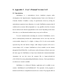
1
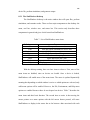
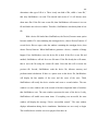
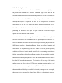
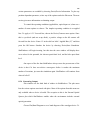
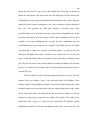
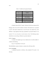
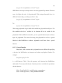
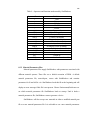
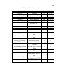
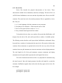
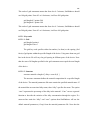
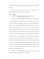
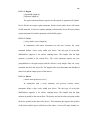
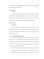
8. Appendix C - User’s Manual Version 1.4.2 8.1 Introduction SimWindows is a semiconductor device simulation program under development at the Optoelectronics Computing Systems Center at the University of Colorado, Boulder. It handles a variety of optoelectronic devices by solving the semiconductor equations in one dimension. As a result, SimWindows assumes that all variables such as current, field and potential, etc. vary parallel to the flow of current but are uniform in the direction perpendicular to the current. Depending on the nature of the device, a one dimensional simulation may or may not be sufficient. To receive announcements concerning new versions of SimWindows, send email to [email protected]. Announcements will be sent only when the version number changes by 0.1 or higher. A change of 0.0.1 in the version number represents bug fixes and interface changes, while changes in physics will receive a version change of 0.1 or higher. SimWindows is freely available over the Internet through the World Wide Web. A web browser such as Netscape or Mosaic can access the home page for SimWindows at http://ucsu.colorado.edu/~winston/simwin.html. Anonymous ftp can also access the program files at hopper.colorado.edu (128.138.248.150) in the pub/modeling/SimWindows directory. Check periodically to see when a new version is available. SimWindows is a Microsoft Windows application and is available in two varieties: SimWindows16 and SimWindows32. The operation of the programs is identical and all files are compatible between the two versions. The programs differ in 122 that SimWindows32 is a “32-bit version” that runs about twice as fast as SimWindows16. This means that SimWindows32 executes instructions and accesses memory using 32 bits instead of 16. Every microprocessor since the 80386 has had the capability of executing 32-bit programs. However, the development tools have only recently become available. Since Microsoft Windows 3.1 and Windows for Workgroups 3.11 are 16 bit applications, these operating systems require the Win32s library. This library does not come with Windows but Microsoft distributes it to developers for their own 32-bit applications. The Win32s library allows 32-bit applications to interface to 16-bit versions of Windows. The library is available on the distribution disks for SimWindows32 and on the same Internet computer site as the SimWindows programs. Windows NT and Windows 95 do not require the Win32s library since they already incorporate the Win32 functionality. As of this writing, SimWindows32 will run on Windows NT and Windows 95 but it has not been thoroughly tested. As with any continuing software project, there are many features that are not yet implemented in SimWindows. The file update.wri lists possible future enhancements. Double clicking on the icon labeled "Future Updates" in the SimWindows group of the Program Manager will access this file. The file consists of three sections: physics, user interface, and user transparent. The physics section consists of enhancements to equations as well as numerical techniques. The user interface section corresponds to the mechanism in which the user manipulates the physics. The user transparent section is the code that helps make the entire program more efficient, manageable, faster etc. SimWindows improves in all of these area 123 simultaneously. There are also release notes that explain the latest features of each version of SimWindows. Double clicking on the icon label “Latest Features” will access the file latest.wri that describes the latest features associated with the version of SimWindows. This file also contains the release notes for all versions of SimWindows. are stored in the file latest.wri. Scroll through this file to see the evolution of SimWindows. 8.1.1 Conventions for this manual There are a few typographical conventions that are of particular importance. The first is the method to describe menu options. The ‘|’ character separates nested menu options. For example: MENU1|Option1|Option2 This means to go to MENU1, select Option1 which will display another menu, and select Option2. The second convention is to denote optional items using []. For example: Option1 Option2 [Option3] This means to perform Option1 and Option2, but Option3 is optional. The third convention is used with keywords in the SimWindows input files. The ‘i’ character denotes that an integer follows the given keyword. The ‘n’character denotes a floating point numerical value. The ‘s’ denotes a string of characters. The string of characters can not contain spaces. The ‘f’character denotes a user function. A list of variables for the function will also follow the ‘f’character. As an example: length=i Nd=n material=s conc=f(x,T) 124 The first example means that an integer must follow “length.” The second example means that a floating point number (or an integer) must follow “Nd.” The third example means a string of characters must follow “material.” The fourth example means that a function of the variables x and T must follow “conc.” This manual assumes that the reader has a working knowledge of Microsoft Windows and are familiar with terms such as “pull-down menus”, “dialog boxes”, “click and drag” and etc. In addition, the reader should have an understanding of the basic file and directory structure of standard MSDOS/Windows based computers. 8.2 Getting Started To start SimWindows just double click on the SimWindows icon from the Program Manager. This starts the simwin16.exe file (simwin32.exe for SimWindows32). Two auxiliary files must be in the same directory as SimWindows. One of those files is the bwcc.dll (bwcc32.dll for SimWindows32). Borland International supplies this file with their compiler. The second file that must be present is material.prm. This file is the default material parameters file for Si and AlGaAs which SimWindows loads when it starts. See section 8.3.2 for more information on material parameters files. SimWindows will generate error messages if neither of these files is present. Both of these files should be present if the installation was successful. SimWindows will now display an introductory screen followed by the desktop window. The following sections comprise a simple tutorial for SimWindows. It begins by outlining the basic interface of SimWindows. It will then explain how to load a 125 device file, perform simulations, and generate output. 8.2.1 The SimWindows Desktop The SimWindows desktop is the main window that will open files, perform simulations, and examine results. There are four major components to the desktop: the menu, tool bar, window area, and status bar. This section only describes these components in general and gives a brief tutorial on SimWindows. Table 7 - List of SimWindows menu items Pull-down menu File Edit Environment Device Plot Data Window Help Purpose File operation commands Edit and search commands for device files Modify environment parameters Modify device and simulation parameters Produce and output plots Input and output misc. data Control layout of windows Display general information about SimWindows With the desktop running, there are three items to observe. First, most of the menu items are disabled, since no devices are loaded. Once a device is loaded, SimWindows will enable most of the menu items. The menu is updated dynamically meaning that depending on which window is active or which options are selected, only valid menu options will be enabled. However, the File, Environment, and Help menu options are enabled because these do not depend on devices. Table 7 describes the menu items and their basic function. The second item to notice is that moving the mouse pointer over menu options with the left mouse button pressed, will cause SimWindows to display in the status bar at the bottom a hint associated with each 126 menu item. The status bar not only displays help hints, but it also displays the current state of the Num Lock and Cap Lock keys on the keyboard. While editing files, the status bar also displays the line number of your cursor. The last item to notice is the tool bar. The tool bar contains buttons that will perform the same function as a particular menu item. Just like the menu, SimWindows updates the tool bar dynamically. When a menu option is enabled, its associated tool button (if any) will be enabled. SimWindows also displays help hints when mouse pointer moves over the various tool buttons. 8.2.2 Loading a Device The first step in using SimWindows is to either load or create a “device file.” There are a number of example device files that come with SimWindows. The device file for this tutorial is comalgpn.dev which is a simple AlGaAs p-n diode. The examples\comments subdirectory for SimWindows contains this file. To load the device file, choose File|Open. This will display the Open File dialog box. The default extension for device files is DEV. Move to the examples\comments subdirectory and open the comalgpn.dev file. SimWindows will create a window which contains the text in the device file. The window itself is called the device window and is one of three kinds of windows that SimWindows uses. The first part of the window caption is “DEVICE FILE” which indicates that this window creates and edits device files. Device files are just ASCII files that contain a description of the device. They contain parameters such as the material, dimensions, and doping. SimWindows can edit many device files simultaneously and the options under the Edit menu can cut and paste selections from one device file to another. When SimWindows opens a file, it 127 determines what type of file it is. There is only one kind of file, called a “state file,” that only SimWindows can read. This tutorial and section 8.3.4 will discuss more about state files. If the file is not a state file, then SimWindows will assume it is a text file and load it into a device window. Therefore, SimWindows can edit any kind of text file. With a device file loaded into SimWindows, the Device|Generate menu option becomes enabled. To start simulating the comalgpn device, choose Device|Generate. If several device files are open, select the window containing the comalgpn device, then choose Device|Generate. When SimWindows generates a device, a number of things happen. First, SimWindows saves the device file to disk. If the file is a new file and untitled, SimWindows will ask for a new file name. If the file already has a file name, then it saves the file using the current file name. Note that this will overwrite the previous file. Second, SimWindows reads the device file, allocates memory and performs initial calculations. If there is a syntax error in the device file, SimWindows will display the line number of the error and the cause of the error. Third, SimWindows will iconify the device window and create a second window. The new window is a state window and is the second of the three important kinds of windows that SimWindows uses. The state window represents the state of the device. Lastly, SimWindows will enable most menu items. If everything was successful, the state window will display the message “Device successfully created.” The state window displays information during device simulations. Simulations are now ready to begin. The iconified device window serves no purpose from here on. 128 8.2.3 Performing Simulations An important item to remember is that SimWindows always completely stores the present state of the device. Each new simulation begins from where the last simulation ended. SimWindows can simulate only one device at a time. It can also save the state of the device on disk. This is done by clicking on the state window and then choosing the File|Save As option. If the state has not been previously saved, then SimWindows will ask for a file name. The default extension for state files is STA. State files store all of the simulation results to let the user examine them later without performing the simulations over again. To open a state file, choose the File|Open option and choose the name of the state file. The initial state of the comalgpn device is charge neutral. This is a non-physical state that SimWindows uses as the initial state for performing device simulations. To return to the initial state, select the Device|Reset option. The first physical state that SimWindows calculates is thermal equilibrium. Choose Device|Start Simulation and SimWindows will begin iterating. The state window shows the present operating conditions and then the iteration number as well as the corresponding numerical error for the iteration. Since solving for equilibrium requires only one variable (potential), the state window displays only one error value. By default the numerical error must be less than 10-8 before the iterations stop. The iterations will also stop if the iteration number reaches the default value of 15. The error, maximum iteration number as well as other parameters are set using Environment|Preferences. When the iterations stop, the state window will display the result of the iteration (converged or not converged), the present device state, and the elapsed time. When the calculation is completed, 129 various parameters are available by choosing Device|Device Information. To plot any position dependent parameter, select any of the options under the Plot menu. The next section gives more information on obtaining output. To control the operating conditions (applied bias, optical input etc.) there are a number of menu options to choose. The simplest operating condition is an applied bias. To apply a 0.5 V forward bias, choose the Device|Contacts menu option. Since this is a pn diode (and not an np diode), a positive voltage on the left contact will forward bias the device. Enter 0.5 in the edit box label “Applied Bias (V)” and then press the OK button. Simulate the device by choosing Device|Start Simulation. SimWindows will begin iterating, but this time the state window will display three error values for the potential, the electron quasi-fermi level, and the hole quasi-fermi level. One aspect of the fact that SimWindows always stores the present state of the device is that if it does not achieve convergence before it reaches the maximum number of iterations, just start the simulation again. SimWindows will continue from where it left off. 8.2.4 Generating Output Plot windows are the third kind of window in SimWindows. The plot menu lists the various options associated with plots. Most of the options from this menu are only available when a device is loaded. The exception to this is the External Optical Spectra plot which SimWindows enables when the environment includes external optical generation. Choose Plot|Band Diagram to see a band diagram of the comalgpn device. To 130 change the scale for the x and y axes, either double click on the plot or choose the Plot|Scale menu option. This will activate the Scale dialog box for the selected plot. This dialog box accepts input for the minimum and maximum x and y values, and gives options for either a linear or logarithmic y axis. Three operations are also available for the y axis. The operations are either none, negative, or absolute value. These operations help to view values that can vary by many orders of magnitude but can also be positive and negative. The best example of this is the recombination rate. It is often desirable to view the recombination on a log plot, but this is problematic since the recombination rate can be both positive a negative. By default plots do not display zero and negative values on a log plot, but selecting either -y or abs(y) in the scale dialog box will display these values. An easier way to set the scale is to use the zoom feature. Click and hold the left mouse button on a plot, then drag a rectangle over the plot. The plot will zoom to the portion within the rectangle and display it in the entire plot area. To return to the automatic scale, choose the Plot|Auto-Scale menu item or press the ESC key. The plot window can also yield actual numerical data in two ways. The first method is the trace window. Select a plot and then choose the Plot|Show Trace Window option. This will display a dialog box associated with the selected plot. When the mouse pointer moves across the plot, the trace window displays the x and y values for the closest data point. Note that each plot has its own trace window. If two plot windows are open, there is a separate trace window for each plot. The second way to obtain data from a plot is to select the plot and choose the File|Save option. SimWindows will ask for a file name and then write the x and y values to the file. The 131 format of the file is comma delimited columns that any typical spreadsheet program can load for further analysis. When plots are visible and SimWindows simulates a device, it also updates the data in the plots automatically to reflect the new results. To prevent this, choose Plot|Freeze Plot. The plot is now frozen with the current data. This feature is useful for displaying two plots of the same quantity for different states of the device different voltages for example. To update a frozen plot, click on the plot window and choose Plot|Melt Plot. 8.2.5 Summary This section has presented a basic look at the functionality of SimWindows. There are a number of items to keep in mind while using SimWindows: 1. Use SimWindows intelligently. It is a software tool just like any other program. If there are problems obtaining convergence, then there may be a problem with the program. The problem may also be related to the nature of the device. For example using too few grid points can cause convergence problems. Play around with your device and submit a bug report if nothing seems to help. 2. Play with SimWindows: There are many subtleties about the user interface that will appear with experience. Submit a bug report if there are suggestions on improving the interface. 3. Be careful when saving: Remember that there are three kinds of windows (device, state, and plot). The File|Save and File|Save As work differently for each one. For a device window, SimWindows saves the device file. Likewise, SimWindows saves the state file when the state window is active. It will save 132 the plot data when a plot window is active. 4. SimWindows always stores the present state of the device: Any time it performs a simulation, it starts from the end of the last simulation. To start from the beginning, choose the Device|Reset option. 8.3 SimWindows File Types SimWindows uses a number of different kinds of files. These files are the material parameters files, device files, state files, and data files. The default extension for each file is PRM, DEV, STA, and DAT respectively, but SimWindows will accept any extension. Material parameters files, device files, and data files are all simple text files while the state file is a binary file that only SimWindows can read. Sections 8.3.2 through 8.3.5 describe each file in detail. Section 8.3.1 describes how to use general purpose functions in SimWindows. 8.3.1 User Functions User functions greatly increase the flexibility of SimWindows by allowing it to accept general functions in material parameters files and device files. This section describes what general functions are and how to input them. Section 8.3.2 will describe how to use general functions in material parameters files and section 8.3.3 will describe how to use general functions in device files. There a three types of user functions: constant, polynomial, and general. They are all interchangeable in that each type of function when can be used when necessary. In order to use any of the types of functions, it is important to know the variables of the function. This manual denotes functions as f(x,y,z) - where x,y, and z are the variables of the function f. Table 8 lists the nine different variables that SimWindows 133 uses. Table 8 - Variables used in general functions Symbol d x T C E G H N A Definition Position Alloy percentage (0-1) Lattice Temperature Carrier Temperature Photon Energy Band Gap Band Gap at 300K Donor Concentration Acceptor Concentration A function denoted by f(x,G) means a function of the alloy percentage and the band gap. Also, the case of the variables is irrelevant. The function f(x,t) is equivalent to f(x,T). Note that the function f(x,t) is not the same as the function f(t,x). This difference is only important when using a polynomial to specify the function f. See section 8.3.1.2 to see why f(x,t) is not the same as f(t,x). The following sections describe how to use each type of function to specify a function f. 8.3.1.1 Constant A constant is the simplest type of a user function, but it is useful to think of a constant as the following: f(x,y,z)=5 is equivalent to 5+0x+0y+0z. When SimWindows requires a function, a constant value will always suffice. 8.3.1.2 Polynomial A polynomial represents an arbitrary order polynomial. The syntax is the following: 134 f(x,y,z)=1,2,3 is equivalent to 1+2x+3x2+0y+0z SimWindows can accept as many terms as necessary separated by commas. The more terms, the higher the order of the polynomial. When using polynomials, there is a difference between f(x,y,z) and f(y,x,z). Here’s why: f(x,y,z)=1,2,3 is equivalent to 1+2x+3x2+0y+0z but: f(y,x,z)=1,2,3 is equivalent to 1+2y+3y2+0x+0z When using polynomials keep in mind which variable the polynomial actually uses. The first variable in the list of variables for the function will be the variable for the polynomial. If this is difficult to remember, just use a general function (next section) to input the polynomial. The reason for having this polynomial as well as a general function is that SimWindows evaluates polynomials much faster than a general function. 8.3.1.3 General Function Many times, both a constant and a polynomial are not sufficient for specifying a function, but SimWindows can interpret and evaluate any algebraic function. For example: f(x,y,z)=(x+y)/z-y^2+2*x is a valid function. Table 9 lists the operators and functions that SimWindows understands. To use pi() and rnd() in a function you have to include the parentheses after the function. f(d)=0.5*cos(2*pi*d/0.5) - invalid function, no parentheses. f(d)=0.5*cos(2*pi()*d/0.5) - valid, parentheses included. 135 Table 9 - Operators and functions understood by SimWindows Operator/Function + * / ^ exp(x) ln(x) sin(x) cos(x) tan(x) asin(x) acos(x) atan(x) atan2(x,y) abs(x) sqrt(x) pi() rnd() Definition Add Subtract Multiply Divide Power Exponential Natural Logarithm Sine (x in radians) Cosine (x in radians) Tangent (x in radians) arcsine (result in radians) arcosine (result in radians) arctangent (result in radians) arctangent of x/y (result in radians) absolute value square root returns pi random number between -1 and 1 8.3.2 Material Parameters Files Material parameters files supply SimWindows with parameters associated with different material systems. These files use a default extension of PRM. A default material parameters file, material.prm, comes with SimWindows and contains parameters for Si and AlxGa1-xAs. SimWindows loads this file at the beginning and will display an error message if this file is not present. Choose Environment|Preferences to set which material parameters file SimWindows loads at startup. Until it loads a material parameters file, SimWindows can not generate a device. SimWindows will also accept new materials in either a modified material.prm file or a new material parameters file. It is advisable to use a new material parameters 136 file instead of modifying material.prm. New versions of SimWindows will overwrite the existing material.prm and erase the changes. Keep in mind that the material.prm is expanding as SimWindows uses new parameters custom material parameters files will often need updating for new versions of SimWindows. To load a custom material parameters file into SimWindows prior to simulating a device, use the Environment|Load Material Parameters menu option. While loading a material parameters file, SimWindows will display an message if the file contains any errors. Material parameters files are simple text files that SimWindows can edit. They must conform to the format outlined in section 8.3.2.1. Section 8.3.2.2 shows the GaAs section of the material.prm file as an example. There are a few general rules that are important when modifying material parameters files: 1. A ‘#’at the beginning of the line comments out any statement. 2. Everything is case insensitive - GrId means the same as Grid. 3. Never use any spaces before or after an '=' or a ','. 4. Every statement must begin in the first column. The material.prm file distributed with SimWindows include comments with additional information on the format of material parameters files. 8.3.2.1 Format The material parameters file consists of an arbitrary number of material sections with one section for each material system. Within each material section there is an arbitrary number of alloy sections. Therefore Si and GaAs would be in different material sections. However, InGaAs and AlGaAs would be in the same material section, but different alloy sections. Each alloy section includes a list of values for each material parameter. The values may either be a simple constant, a general function, or 137 employ a built-in model for the parameter. Adding new material or alloy sections can expand the material parameters file. There are no limits as to the type of materials and therefore SimWindows can handle any material system. The following sections describe the keywords and syntax for material parameters files. 138 Table 10 - SimWindows material parameters Symbol Band_Gap Electron_Affinity Static_Permitivity Refractive_Index Absorption Thermal_Conductivity Deriv_ Thermal_Conduct Electron_Mobility Hole_Mobility Eelectron_Dos_Mass Hole_Dos_Mass Electron_Cond_Mass Hole_Cond_Mass Electron_Shr_Lifetime Hole_Shr_Lifetime Rad_Recomb_Const Electron_Energy_Lifetime Hole_Energy_Lifetime Qw_Rad_Recomb_Const Electron_Collision_Factor Hole_Collision_Factor Meaning Band gap Electron affinity Electrostatic permitivity Refractive index Optical absorption Thermal conductivity Thermal conductivity derivative wrt. temperature Electron mobility Hole mobility Electron density of states mass Hole density of states mass Electron conductivity mass Hole conductivity mass Electron SHR lifetime Hole SHR lifetime Radiative recombination constant Electron energy relaxation lifetime Hole energy relaxation lifetime Radiative recombination constant when used in a QW. Electron scattering coefficient (-1/2,0,1/2,3/2) Hole scattering coefficient (-1/2,0,1/2,3/2) Unit Variables eV x,T eV x, T (none) x (none) x,T,E,G,H -1 cm x,T,E,G,H W K-1 cm-1 x,T -2 -1 W K cm x,T cm2 V-1 s-1 cm2 V-1 s-1 (none) x,T,C,N,A x,T,C,N,A x (none) x (none) x (none) s s cm3 s-1 x x x x s x s x cm2 s-1 x (none) x (none) x 139 8.3.2.1.1 Material Section Material=s The material keyword starts a material section. Device files will select the material by using the specified name of the material, s. The name can not contain spaces. 8.3.2.1.2 Alloy Section Alloy=default Alloy=s To specify different alloys for a particular material, use the alloy keyword. Device files will select the alloy by using the specified name of the alloy, s. As with the material keyword, the name of the alloy can not contain spaces. If the material has default parameters that apply if the device file does not specify an alloy, then use “Alloy=default.” Each material section can have any number of alloys for that material. The material parameters file can reuse the names of alloys if they are in different material sections. 8.3.2.1.3 Material Parameters There are presently 21 material parameters that the material parameters file must specify for each material-alloy combination. Table 10 lists the keywords for each material parameter. Each alloy in the material parameters file must use each keyword or an error message will result. Each keyword must use a function (constant, polynomial, or general function) to specify the value of the material parameter. Each function is function of certain variables and Table 10 also lists those variables. Keeping in mind that each material parameter is a function of particular variables, there are two ways to specify the value of a material parameter. The first is 140 to specify one function that is valid for all values of the variables. The second is to specify different functions that apply for different ranges of input variables. The following sections describe each of the methods. 8.3.2.1.3.1 Single Function If a single function is sufficient to specify a material parameter, then use just one line for the material parameter. Some examples using the band gap follow. Remember that the band gap is a function of the alloy percentage (x) and the lattice temperature (T). BAND_GAP Value=1.424 This specifies a constant value for the band gap that is valid for all values of x and T. BAND_GAP Value=1.424,1.247 This example specifies to use a polynomial for the value of the band gap. This is equivalent to 1.424+1.247*x+0*T. BAND_GAP Value=1.424+1.25*x-5.4e-4*(T^2/(T+204)-300^2/(300+204)) This is a general function for the band gap as a function of x and T. 8.3.2.1.3.2 Piecewise Function A piecewise function can specify different functions that are valid over different ranges of the variables. Some examples, again using the band gap, follow: BAND_GAP Segments=2 Start_x=0.00 end_x=0.45 start_t=0 end_t=0 value=1.424,1.247 Start_x=0.45 end_x=1.00 start_t=0 end_t=0 value=1.9,0.125,0.143 On line 1, “segments” specifies the number of different functions that will follow. On line 2, “value” specifies the actual function. “Start_x” and “end_x” specify the range of x for which the value function is valid. Since the band gap is a function of T as well, 141 use a “start_t” and an “end_t” to specify the ranges of T. In this case “start_t” and “end_t” are both zero meaning that the value function is valid over all T. If the line does include a start and end value, then SimWindows assumes that the function is valid over the entire range of the variable. Therefore, “start_t” and “end_t” statements in line 2 are not necessary. In summary, line 2 means to give the band gap a value of 1.424+1.247*x for 0.00<x<0.45 and for all T. Line 3 is the same as line 2 except that it uses a different function for 0.45<x<1.00. An important feature of the start and end values is that they can also be functions not just numbers. For example, since the band gap is a function of x and T, the start and end values for both x and T, can be functions of x and T. An example using the absorption of GaAs: ABSORPTION Segments=2 start_e=0 end_e=g value=0 start_e=g end_e=100 value=3.5e4*(e-g)^0.5 For a photon energy (e) between 0 and the band gap (g) the absorption coefficient will be 0. For a photon energy between the band gap and 100, the absorption will be 3.5e4*(e-g)^0.5. 8.3.2.1.3.3 Built-in Models In addition to general functions, several “built-in” models for material parameters are available. Built-in models are just functions of a certain form for which the user specifies the coefficients. Built-in models are available for the electron affinity, band gap, mobility, thermal conductivity, derivative of the thermal conductivity with respect to temperature, optical absorption, and the index of refraction. Only certain models apply to certain material parameters and SimWindows will display a message 142 when a model is not applicable to the material parameter. The syntax for a built-in model is: MATERIAL_PARAM Model=model_name terms=a,b,c,d,e where “MATERIAL_PARAM” is the name of the material parameter, “model_name” is the name of the model, and “a,b,c,d,e” are the coefficients that SimWindows uses in the model. Each model uses a different numbers of coefficients, and SimWindows will display a message if there is an incorrect number of coefficients for the model. Each of the following sections describes the various built-in models. 8.3.2.1.3.3.1 Band Gap Model name: Band_gap T2 300 2 function: f (x , T ) = a + bx + cx 2 + d − e + T e + 300 Material Parameter: BAND_GAP, ELECTRON_AFFINITY This model simply allows for the variation in the band gap with respect to temperature. At T=300K, the model reduces to a second order polynomial relationship between the alloy percentage and the band gap. This model is valid for the electron affinity in order to control how the band gap narrowing is divided between the conduction and valence bands. 8.3.2.1.3.3.2 Thermal Conductivity Model name: Thermal_conduct a function: f (x , T ) = Te 2 b + cx + dx Material Parameter: THERMAL_CONDUCTIVITY, DERIV_THERMAL_CONDUCT This model allows for the variation of the thermal conductivity with respect to the alloy percentage and the lattice temperature. The derivative of this relation with respect to the temperature yields another relation of the same form. 143 8.3.2.1.3.3.3 Mobility Model name: Mobility Ci 2 f gx hx + + + ( ) 1 + N + A j Material Parameter: ELECTRON_MOBILITY, HOLE_MOBILITY ( function: f ( x, T , C , N , A) = a + bx + cx 2 ) C e d ( ) C k (d ) ( ) This model applies to the electron and hole mobilities to control their variation with respect to the alloy concentration (x), the lattice temperature (T), the carrier temperature (C), and the doping concentrations (N-donors, A-acceptors). Note that this model does not explicitly use the lattice temperature, but rather the carrier temperature. Under most circumstances the carrier temperature is the same as the lattice temperature. However, the mobilities can depend on the lattice temperature and a user function that uses T as a variable is applicable. 8.3.2.1.3.3.4 Absorption Model name: Power_absorption e function: f (x , T , E , G ) = ( a + bx + cx 2 )( E − d ) Material Parameter: ABSORPTION Model name: Exp_absorption function: f (x , T , E , G ) = a exp(b( E − c)) Material Parameter: ABSORPTION These two models are analytical expressions that relate the photon energy to the absorption coefficient. There is no temperature dependence in these models, but a user function can include the temperature. Model name: Power_band_gap_absorption e function: f (x , T , E , G ) = (a + bx + cx 2 )(E − G − d ) Material Parameter: ABSORPTION Model name: Exp_band_gap_absorption function: f (x , T , E , G ) = a exp(b (E − G − c)) Material Parameter: ABSORPTION 144 These two models are the same as the first two except for the incorporation of the bulk band gap. Since the band gap can vary as a function of temperature, these absorption models will also vary with temperature. 8.3.2.1.3.3.5 Refractive Index Model name: Oscillator_refractive_index function: Internal (no coefficients required) Material Parameter: REFRACTIVE_INDEX This is a special model that requires no terms and is applicable to AlxGa1-xAs only. It appears and was reported in J. Appl. Phys. (70) 1, 1 July 1991 by Terry. This is dependent on the aluminum percentage in the alloy. It is also dependent on the temperature through the temperature dependence of the band gap. 8.3.2.2 Example Material Section The following is the GaAs section of the material.prm that comes with SimWindows. It shows how to use the various keywords described in the previous sections. Material=GaAs Alloy=Default Band_gap Model=Band_gap terms=1.424,0,0,-5.405e-4,204 Electron_affinity Model=Band_gap terms=4.07,0,0,2.702e-4,204 Static_permitivity Value=13.18 Refractive_index Model=oscillator_refractive_index Absorption Segments=2 start_e=0 end_e=g+0.00087 model=exp_band_gap_absorption terms=1,71,0.104 start_e=g+0.00087 end_e=100 model=power_band_gap_absorption terms=3.5e4,0,0,0,0.5 Thermal_conductivity Model=Thermal_Conduct terms=549.356,1,0,0,-1.25 Deriv_thermal_conduct Model=Thermal_Conduct terms=-686.695,1,0,0,-2.25 Electron_mobility Value=8000 Hole_mobility Value=370 Electron_dos_mass Value=0.067 Hole_dos_mass Value=0.62 Electron_cond_mass Value=0.067 145 Hole_cond_mass Value=.62 Electron_shr_lifetime Value=1e-8 Hole_shr_lifetime Value=1e-8 Rad_recomb_const Value=1.5e-10 Electron_energy_lifetime Value=1.e-12 Hole_energy_lifetime Value=1.e-12 Qw_rad_recomb_const Value=1.54e-4 Electron_collision_factor Value=0.5 Hole_collision_factor Value=0.5 Alloy=Al Band_gap Segments=2 Start_x=0.00 end_x=0.45 Model=Band_gap terms=1.424,1.247,0,-5.405e-4,204 Start_x=0.45 end_x=1.00 Model=Band_gap terms=1.9,0.125,0.143,-5.405e-4,204 Electron_affinity Segments=2 Start_x=0.0 end_x=0.45 Model=Band_gap terms=4.07,-0.7482,0,2.702e-4,204 Start_x=0.45 end_x=1.0 Model=Band_gap terms=3.594,0.3738,-0.143,2.702e-4,204 Static_permitivity Value=13.18,-3.12 REFRACTIVE_INDEX Model=oscillator_refractive_index Absorption Segments=2 start_e=0 end_e=g+0.00087 model=exp_band_gap_absorption terms=1,71,0.104 start_e=g+0.00087 end_e=100 model=power_band_gap_absorption terms=3.5e4,0,0,0,0.5 Thermal_conductivity Model=Thermal_Conduct terms=549.356,1,12.7,-13.22,-1.25 Deriv_thermal_conduct Model=Thermal_Conduct terms=-686.695,1,12.7,-13.22,-2.25 Electron_mobility Segments=2 Start_x=0.0 end_x=0.45 Value=8000,-22000,10000 Start_x=0.45 end_x=1.0 Value=-255,1160,-720 Hole_mobility Value=370,-970,740 Electron_dos_mass Value=0.067,0.083 Hole_dos_mass Value=0.62,0.14 Electron_cond_mass Segments=2 Start_x=0.0 end_x=0.45 Value=0.067,0.083 Start_x=0.45 end_x=1.0 Value=0.32,-0.06 Hole_cond_mass Value=0.62,-0.14 Electron_shr_lifetime Value=1e-8 Hole_shr_lifetime Value=1e-8 Rad_recomb_const Value=1.5e-10 Electron_energy_lifetime Value=1.e-12 Hole_energy_lifetime Value=1.e-12 Qw_rad_recomb_const Value=1.54e-4 Electron_collision_factor Value=0.5 Hole_collision_factor Value=0.5 146 8.3.3 Device Files Device files describe the physical characteristics of the device. These characteristics include device dimensions, materials, and doping. The device file is an ASCII file that SimWindows can create and edit. By default device files use the DEV extension. The same basic rules for material parameters files are applicable to device files. They are: 1. A ‘#’at the beginning of the line comments out any statement. 2. Everything is case insensitive - GrId means the same as Grid. 3. Never use any spaces before or after an '=' or a ','. 4. Every statement must begin in the first column. To describe the device, there are a number of keywords that SimWindows will interpret from the device file, and each keyword has a number of available options. The following section describes each keyword that SimWindows understands. Many keywords have a number of variations that the same device file can mix with the other variations. Most statements are optional in the device file, but every device file must contain at least one grid statement, one structure statement, and one doping statement. The total length for all of the grid statements, structure statements and doping statements must be equal (which represents the total length of the device). The order of statements in the device file is very important for statements using the same keyword. Since the length parameter describes the length for a particular statement, SimWindows applies them in the order that they appear in the device file. For example: grid length=0.5 points=100 grid length=0.3 points=200 147 This order of grid statements means that from 0 to 0.5 microns, SimWindows should use 100 grid points. From 0.5 to 0.8 microns, it will use 200 grid points. grid length=0.3 points=200 grid length=0.5 points=100 This order of grid statements means that from 0 to 0.3 microns, SimWindows should use 200 grid points. From 0.3 to 0.8 microns, it will use 100 grid points. 8.3.3.1 Keywords 8.3.3.1.1 Grid grid length=f points=i grid length=f size=f The grid key word specifies either the number (1st form) or the spacing (2nd form) of grid points within the specified length of the device. Using more than one grid line in the device file will vary the grid spacing in different parts of the device. Note that the sum of all lengths specified in the grid statements must equal the total length of the device. 8.3.3.1.2 Structure structure material=s length=f [ alloy=s conc=f(d) ] The structure statement defines the material composition for a specified length of the device. The material parameters file must contain the specified material name. If the material has an associated alloy name, then “alloy” specifies the name. The option “conc” represents the percentage of the alloy in the material. “Conc” can use a general function to describe the variation of the alloy concentration through the region. If a structure line omits the “alloy” and “conc” options then SimWindows will use the default material parameters (if any) from the material parameters file. Note that the 148 sum of all lengths specified in the structure statements must equal the total length of the device. Note that for every structure statement, d starts at 0. Do not consider in the function f(d) where in the device the structure actually starts. 8.3.3.1.3 Doping doping length=n [ Nd=f(d) ] [ Na=f(d) ] [Nd_deg=i] [Na_deg=i] [Nd_level=f(d)] [Na_level=f(d)] The doping statement defines different doping regions. The “length” parameter specifies the length of the region. The “Nd” and “Na” parameters specify the donor and acceptor concentration respectively. These can use a general function f(d) to describe the variation of the doping density through the region. If the statement omits both doping concentrations, then it uses an intrinsic material. The “Nd_deg” and “Na_deg” parameters specify the degeneracy factor for the dopant. Incomplete ionization of dopants uses the degeneracy factor. The value is usually 2 for donors and 4 for acceptors. If the statement omits either of these parameters, then SimWindows uses a default value of 0 meaning complete ionization of dopants. The parameters “Nd_level” and “Na_level” specify the energy level of the dopant in eV. A positive value for these parameters means that the energy level is in the band gap (the donor level is below the conduction band and the acceptor level is above the valence band). If the statement omits either of the parameters, then SimWindows uses a default value of 0. As with the grid and structure statements, the total length of the doping regions must equal the total length of the device. Note that for every doping statement, d starts at 0. Do not consider in the function f(d) where in the device the structure actually starts. 149 8.3.3.1.4 Region [region bulk length=n] [region qw length=n] The region statement denotes regions as bulk regions or quantum well regions. Device files do not require region statements. In this case the entire device will consist of bulk materials. If a device contains quantum wells then the device file must contain region statements for both the quantum well and bulk regions. 8.3.3.1.5 Cavity [ cavity surface area=n length=n] In conjunction with mirror statements (see the next section), the cavity statement defines a laser cavity within your device. The only type of cavity that SimWindows supports is for surface emitting lasers. This implies that the light emission is parallel to the current flow. The cavity statement requires the area (perpendicular to the light output) and the effective cavity length. Only one cavity statement may be in the device file. The length of the cavity determines the distributed mirror loss and the output power of the mirrors. 8.3.3.1.6 Mirror [ mirror metal position=n ref=n ] In conjunction with a cavity statement (see previous section), mirror statements define a laser cavity within your device. The only type of cavity that SimWindows supports is for surface emitting lasers. This implies that the light emission is parallel to the current flow. The mirrors are placed at discrete points within the device (usually at the ends of the device). This statement only requires the position of the mirror and the power reflectivity of the mirror. A device file must include two 150 mirror statements for laser simulations, SimWindows will compute the electromagnetic field profile only between the mirrors. 8.3.3.1.7 Radius [ radius=n ] The radius statement defines the radius of your device. SimWindows assumes that all devices are cylindrical. The default radius is one micron if a device file omits the radius statement. Only the lateral heat flow model in SimWindows uses the radius parameter. It is only necessary when using this model in thermal simulations. 8.3.3.1.8 Repeat [ repeat start ] [ repeat=n ] The repeat statement allows a device file to specify periodic structures. Use the “repeat start” statement before any group of statements, and then use the “repeat=n” after the group of statements. SimWindows will repeat these statements for the specified number of times. 8.3.3.2 Overriding Material Parameters In addition to specifying the device structure, the device file can also contain overrides of any of the material parameters. This means that any device file can use a new value for a material parameter and not use the default value that is in the material parameters file. To do this use exactly the same syntax that appears in the material parameters file with the following additions: 1. On the first line for the material parameter, include a length=n option where n is the length for which the override will apply. Use multiple lines to override the material parameter differently for different parts of the device, but override the 151 material parameter over the entire device. 2. In addition to the regular variables for the material parameter, a general function can also use the variable d (position) for the material parameter. This provides a position dependent material parameter. For example, the material parameters file specifies the band gap according to: BAND_GAP Value=f(x,T) In the device file, the statement would be: BAND_GAP length=n value=f(x,T,d) 8.3.3.3 Example Device Files The following is an example device file that comes with SimWindows. It is a simple AlGaAs p-n diode. It uses a number of grid statements to adjust the grid spacing through the device. It has two structure statements to vary the Al composition of the device, and it specifies a position dependent doping concentration. # The grid lines are used to specify the number of grid points in # a particular region. Instead of using "points" you can also use # "size=" to specify the spacing between grid points. grid length=.450 points=25 grid length=.049 points=40 grid length=.002 points=40 grid length=.049 points=40 grid length=.450 points=25 # The structure lines are used to specify the material, alloy, and alloy #composition. # The names for material= and alloy= must correspond to names in the # material parameters file. It is not necessary to specify an alloy. # If no alloy is specified then the default material parameters (specified # material.prm) are used. structure material=gaas alloy=al length=0.50 conc=0.40 structure material=gaas alloy=al length=0.50 conc=0.00 # The doping lines are just used to specify the doping. If no doping is # specified then the region is intrinsic. doping length=.500000 Na=1e+17-5e16/0.5*d doping length=.500000 Nd=5e+16+5e16/0.5*d 152 8.3.4 State Files Since device simulations can be a time consuming task, state files can save results for later examination. A state file contains all of the data that is in memory. As a result state files can be quite large depending primarily on the number of grid points in the device. State files are binary files that only SimWindows can interpret. To save a state file click on the state window of your device and choose the File|Save As menu option. SimWindows will ask for a filename. The default extension for state files is STA. If the state file already has a file name, just choose the File|Save menu option and SimWindows will save the state file to the old filename. To restore a state file, use the File|Open menu option and select the state file to open. If a device already exists, SimWindows will prompt to save the results of that device. If SimWindows opens the state file successfully, the message “Device successfully created” will appear in the state window. The device will be in exactly the same state as when SimWindows saved it. 8.3.5 Data Files SimWindows can also generate data files that contain the numerical values of any desired data. Plots can generate data files directly by selecting a plot on the screen, and choosing the File|Save As option. After entering a file name, SimWindows will output the data to the file. Also use the menu items under the Data pull down menu to output non position dependent data or to create custom sets of data. Data files are always ASCII files that any standard word processor or spreadsheet can read. The data is comma delimited which makes it difficult to read on the screen. However it is easy to load the data into a spreadsheet program that accepts 153 comma delimited text. The resulting spreadsheet will be easy to read and manipulate. 154 8.4 Bug Report In an effort to increase the stability and usefulness of SimWindows, the following bug report can be used to report any problems that you encounter. Many problems result from the configuration of your system and are very difficult for me to test. Therefore, I strongly encourage you to fill out a bug report. You may send it by U.S. mail, fax, or e-mail to the following address: David W. Winston Dept. of Computer and Electrical Engr. Campus Box 425 University of Colorado Boulder CO 80309-0425 Fax: (303) 492-3674 e-mail: [email protected] Bug type: System Crash - SimWindows caused Windows to crash or required reboot. SimWindows Crash - SimWindows crashed but did not affect Windows programs. Program Error - You noticed a bug in SimWindows. Description: Describe in as much detail as possible what happens: 155 Error Messages: If there were any error messages what exactly did it say (include descriptions of dialog box captions and buttons that were available): Misc. Questions: Can you repeat the problem: Yes No If so, what procedure will reproduce the problem: What Version of SimWindows do you use (use Help|About): When was it last modified (use Help|Last Updated): Which version of Windows do you use: Which processor do you have: Clock speed: List other programs (if any) that were running when you executed SimWindows: 156 8.5 Class Diagrams The following class diagrams depict the class structure for SimWindows version 1.4.2. Classes are essentially modules that combine data and functionality. In object oriented programming, classes can be “derived” from other classes. This means that the derived classes “inherit” the data and functionality of the parent classes while adding some data and functionality of its own. The following figure shows the legend of symbols used by the class diagrams. Class Name File Name Abstract Class A B B is a friend class of A A B B is a derived class from A A B B is pointed to by A (not all pointers are shown) Borland Supplied OWL 2.5 Class Figure 46 - Symbols used in class diagrams The following six figures comprise the class structures for SimWindows. Figure 47 shows the main classes that create the various windows in the user interface. Figure 48 presents the classes that create all of the dialog boxes. Figure 49 shows various support classes. The validator classes in this figure are used to verify the input to edit controls. Figure 50 shows the material storage, material, and alloy classes. This figure also shows various function and physical models classes. Figure 51 presents the device and grid related classes. Figure 52 shows the corresponding solution and element classes. 157 TApplication TMDIClient TSimWindows simwin.cpp TSimWindowsMDIClient simclien.cpp TPrintOut TPrintEditFilePrintOut simedit.cpp TPlotPrintOut simplot.cpp TEditFile TWindow TPrintEditFile simedit.cpp TSimWindowsPlot simplot.cpp TSimWindowsEditFile simedit.cpp TSimWindowsDeviceStatus simedit.cpp TSimWindowsEnvironPlot simplot.cpp TSimWindowsMacroPlot simplot.cpp TSimWindowsBandDiagram simplot.cpp Figure 47 - Main Windows interface classes TDialog TCenterDialog simcdial.cpp TDialogTrace simcdial.cpp TDialogSelectOneParameter simcdial.cpp TDialogOpticalInput simdial.cpp TDialogSelectParameters simcdial.cpp TDialogDeviceContacts simdial.cpp TDialogPreferences simcdial.cpp TDialogDeviceSurface simdial.cpp TDialogSelectMacro simcdial.cpp TDialogElectricalModels simdial.cpp TDialogVoltageMacro simcdial.cpp TDialogThermalModels simdial.cpp TDialogDeviceInfo simcdial.cpp TDialogLaser simdial.cpp TDialogScale simcdial.cpp TDialogWriteBand simdial.cpp TDialogAbout simcdial.cpp TDialogDataWriteAll simdial.cpp Figure 48 - Dialog box classes 158 TParse parclass.cpp TMacroStorage macclass.cpp TPreferences supclass.cpp TParseMaterialParam parclass.cpp TMacro macclass.cpp TErrorHandler supclass.cpp TParseDevice parclass.cpp TParseMaterial parclass.cpp TVoltageMacro macclass.cpp TFlag supclass.cpp TValueFlag supclass.cpp TValidator TEffectFlag supclass.cpp TFilterValidator TMustEnterValidator simvalid.cpp TScientificUpperValidator simvalid.cpp TValueFlagWithObject supclass.cpp TScientificRangeValidator simvalid.cpp TScientificLowerValidator simvalid.cpp Figure 49 - Support and text validator classes TMaterialStorage matclass.cpp TMaterial matclass.cpp TAlloy matclass.cpp TMaterialParamModel matclass.cpp TDeviceFileInput infclass.cpp TPieceWiseFunction funclass.cpp TFunction funclass.cpp TPolynomial funclass.cpp TUserFunction funclass.cpp TModelMobility funclass.cpp TConstant funclass.cpp TModelBandGap funclass.cpp TTermsFunction funclass.cpp TModelAlGaAsPermitivity funclass.cpp TModelThermalConductivity funclass.cpp TModelPowerAbsorption funclass.cpp TModelPowerAbsorptionBandGap funclass.cpp TModelAlGaAsRefractiveIndex funclass.cpp TModelExpAbsorption funclass.cpp TModelAlGaAsAbsorption funclass.cpp TModelExpAbsorptionBandGap funclass.cpp Figure 50 - Material and function classes 159 TEnvironment envclass.cpp TDeviceFileInput infclass.cpp TDevice devclass.cpp TSolution solclass.cpp TCavity cavclass.cpp TMirror mirclass.cpp TContact conclass.cpp TMode modclass.cpp TSurface surclass.cpp Node Structure TNode nodclass.cpp TElectron carclass.cpp THole carclass.cpp TBoundElectron bdcclass.cpp TFreeElectron frcclass.cpp TGrid grdclass.cpp TQuantumWell qwclass.cpp TBoundHole bdcclass.cpp TFreeHole frcclass.cpp T2DHole 2dcclass.cpp T2DElectron 2dcclass.cpp Figure 51 - Device and node classes TSolution solclass.cpp TDevice devclass.cpp Element Structure All classes except TElement are friends of TNode TElement eleclass.cpp TElectricalElement elcclass.cpp TBulkElectricalElement elcclass.cpp TElectricalServices eleclass.cpp TQWElectricalElement elcclass.cpp TOhmicBoundaryElement elcclass.cpp TThermalElement thrclass.cpp TBulkThermalElement thrclass.cpp TQWThermalElement thrclass.cpp TBoundaryThermalElement thrclass.cpp Figure 52 - Element classes