Download MATLAB 4.0 & SIMULINK 1.2c PRIMER for the Microsoft Windows

1
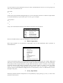
MATLAB 4.0 & SIMULINK 1.2c PRIMER
for the
Microsoft Windows Environment
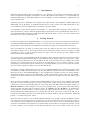
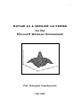
The Mexican "Sombrero"
1
0.8
0.6
0.4
0.2
0
-0.2
-0.4
40
40
30
30
20
20
10
10
0
0
Prof. Evangelos Papadopoulos
Fall, 1995
2
Table of Contents
1.
Introduction
3
2.
Getting Started
3
3.
The HELP Facility
4
4.
Workspace Management
5
5.
The MATLAB Matrix
5
6.
Matrix Operations
7
7.
Array Operations
7
8.
Graphics
9
9.
Environment Controls
12
10.
Polynomial Operations
12
11.
System Models and Response
13
12.
Logical Operations
15
13.
Control Flow
16
14.
Function M-Files
17
15.
Script M-Files
18
16.
SIMULINK
19
3
1.
Introduction
MATLAB, which stands for MATrix LABoratory, is an interactive programming environment for high-level
numeric computation and graphic visualization. Its basic data element is the matrix so it is assumed that any
individual endeavoring to learn MATLAB has a basic knowledge of matrix mathematics obtained from any
Linear Algebra course.
The following primer is intended as a brief guide to the major functions and capabilities of MATLAB 4.0 and
SIMULINK 1.2c for Windows. To understand the full power of this software, the reader should refer to the
User’s Manual or peruse the HELP facility (see Chapter 3 for more details).
It is important to note that the Windows Environment is a menu-driven disk operating system whereby the
major input device is a mouse. When using MATLAB, many operations can be performed using either menu or
line commands. Both methods will be described where appropriate and it is left to the user to decide which
method he or she is more comfortable with.
2. Getting Started
In order to run MATLAB 4.0 and SIMULINK 1.2c, you must open an account at the Vectra Lab in room G-01
in the Macdonald-Harrington Building. For those of you who have never opened an account in the Vectra Lab,
the procedure is quite simple and you should have no problems so long as your tuition fees have been paid.
Once you find the lab, jot down its working hours which are posted on the door. Next, enter and find any
unoccupied computer. This is any computer which has the F:\LOGIN> prompt. Above the prompt are listed
instructions on how to open an account and how to login once your account has been validated. These
instructions have been repeated below.
To open an account, type NEWUSER at the prompt and press enter. Follow the instructions on the screen. Once
you have finished answering all the questions, you should get back the original login screen and prompt. At this
point, go to the front desk with your ID card and $5.00. One of the lab supervisors will validate your account
and give you a receipt. While you are at the desk you can add money to your account for printing. It costs
$0.10/page to print on the laser printer in the lab so it is recommended that you pay an extra $1.00 for printing
since you will be expected to submit your results from MATLAB.
The Windows version of MATLAB can only be run on the Hewlett-Packard Pentium and 486 computers which
are found in the middle and extreme right of the lab. The IBM 386 machines can only run MATLAB 3.5j for
DOS. Room 283 in the Macdonald Building is also equipped with computers but they are mostly HewlettPackard 286 machines, which also have MATLAB 3.5j, and some MUSIC terminals thrown in. Nevertheless,
you have access to these computers with your account and it is open 24 hours/day. The door code will be given
in class.
Once you find a free computer, sit down and type LOGIN EMF/your login name at the F:\LOGIN> prompt and
press enter. The system will prompt you for your password. For security reasons, your password will not be
echoed on the screen so type carefully and press enter when done. The Main Menu will appear. Choose 7 )
Math & Statistics by either using the arrow keys and pressing enter or by moving the mouse and clicking.
Another window will appear with four choices. Choose 3) Matlab 4.0 for Windows. As MATLAB is
being loaded into primary memory, another window will appear stating that the file progman.ini is writeprotected and that the default settings will not change after you finish your session. Click on the OK box to
proceed with the loading operation. You should get the Command Window with the characteristic MATLAB
prompt “»” in order to begin your session.
Please note that since there are only 38 Hewlett-Packard machines to go around, it will be quite difficult to find a
free computer as the term progresses so one solution is to be present at the lab as soon as it opens for the day. If
you cannot get up early enough for the opening of the lab or if you have a course to attend, another solution
would be to write M-Files (see Chapters 14-15) at home using any text editor or word processor and once you do
get a free computer, you can simply run your M-Files and print a copy of your results. In this way, you can
4
spend your time in the lab debugging on-line, interpreting your results, and optimizing your work instead of
wasting your (and other people’s) time typing.
3. The HELP Facility
The simplest way to invoke MATLAB’s instructional HELP facility is to click on the Help menu item. A
pull-down window will appear. If you click on Table of C ontents..., a list of the directory names where
MATLAB related files are grouped appears. Clicking on one of the directories will present a list of the functions
in that directory. By clicking on a function, a brief description and the syntax required to implement it will be
shown.
If you want a list of all the functions available on MATLAB without having to find the directory to which it
belongs, simply click on Index... from the Help pull-down window then click on the function to find out
more about it. To quit the HELP facility click on F ile then E x it from the MATLAB Help WIndow.
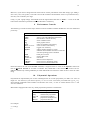
An equivalent method of getting on-line assistance is to type help and press enter at the command prompt. A
list of the directories as described above will scroll down the screen as shown below:
» help
HELP topics:
c:\matlab
matlab\general
matlab\ops
matlab\lang
matlab\elmat
matlab\specmat
matlab\elfun
matlab\specfun
matlab\matfun
matlab\datafun
matlab\polyfun
matlab\funfun
matlab\sparfun
matlab\plotxy
matlab\plotxyz
matlab\graphics
matlab\color
matlab\sounds
matlab\strfun
matlab\iofun
matlab\demos
simulink\simulink
simulink\blocks
simulink\simdemos
nnet\examples
nnet\nnet
toolbox\control
-
Establish MATLAB session parameters.
General purpose commands.
Operators and special characters.
Language constructs and debugging.
Elementary matrices and matrix manipulation.
Specialized matrices.
Elementary math functions.
Specialized math functions.
Matrix functions - numerical linear algebra.
Data analysis and Fourier transform functions.
Polynomial and interpolation functions.
Function functions - nonlinear numerical methods.
Sparse matrix functions.
Two dimensional graphics.
Three dimensional graphics.
General purpose graphics functions.
Color control and lighting model functions.
Sound processing functions.
Character string functions.
Low-level file I/O functions.
Demonstrations and samples.
SIMULINK model analysis and construction functions.
SIMULINK block library.
SIMULINK demonstrations and samples.
Neural Network Toolbox examples.
Neural Network Toolbox.
Control System Toolbox.
For more help on directory/topic, type "help topic".
»
By typing help directory name, all the functions in that directory will scroll down the screen. To get quick
information on functions, including user-created functions, simply type help function. Please refer to Chapter
14 for more information on how to include help information for your own functions.
5
4. Workspace Management
There are three ways to quit MATLAB. You can either type quit or exit at the command prompt and press
enter or click once on F ile then on E x it MATLAB.
Before quitting the workspace, it is a good idea to save it for future reference. From the F ile pull-down window,
choose Save Workspace A s . . . . Under the Driv es: selection box, change the hard-disk location to f :
emf/home:your login name . This is done by clicking on the up arrow icon next to the Driv es: box until
you see your directory scroll on the screen. Select it by clicking once on it. Now type the name of your filename
where you see *.mat. The extension .mat will be added if you do not include it yourself after typing the
filename. Click on the OK box.
Everyone is allotted 5MB of free disk space which should be sufficient for your work but you still should
transfer all your files to portable 1.44MB diskettes just in case something happens. To do this, just change the
Driv es: location to a: before saving the file. To store files directly from the Command Window simply type
save (disk location a or f):\filename. If you do not want to save all your MATLAB variables in the workplace,
simply type save (disk location a or f):\filename variable1 variable2 etc. so that only variable1, variable2,
etc. will be stored.
To retrieve your workspace type load (disk location a or f):\filename without the .mat extension and press
enter.
5. The MATLAB Matrix
The simplest way to enter a matrix is by using an explicit list as shown below:
» A=[1 sqrt(2) 3+j; 4 5 6-4*i; (7-2)*4/5+3 8.3 -9]
A=
1.0000
1.4142
3.0000 + 1.0000i
4.0000
5.0000
6.0000 - 4.0000i
7.0000
8.3000
-9.0000
Equivalently, the following could have been entered:
» A=[1 sqrt(2) 3+j
4 5 6-4*i
(7-2)*4/5+3 8.3 -9]
A=
1.0000
1.4142
4.0000
5.0000
7.0000
8.3000
3.0000 + 1.0000i
6.0000 - 4.0000i
-9.0000
As the above example demonstrates, the matrix elements can be either real or complex (with i and j being
interchangeable) or expressions such as sqrt(2) and (7-2)*4/5+3.
All matrices, including scalars (1x1) and vectors (1xn or mx1), are indexed in the same fashion as shown below:
(1,1)
(2,1)
(3,1)
.
.
.
(m,1)
(1,2)
(2,2)
(3,2)
.
.
.
(m,2)
(1,3)
(2,3)
(3,3)
.
.
.
(m,3)
...
...
...
...
...
...
...
(1,n)
(2,n)
(3,n)
.
.
.
(m,n)
So, if you want the element (2,3) of matrix A, simply enter the following:
6
» B=A(2,3)
B=
6.0000 - 4.0000i
If you had two vectors V=[1 -6 7 9E2 22] and W=[1; 2; 3; 4e3; 0] then:
» C=V(4)
C=
900
» D=W(4)
D=
4000
For row vectors, it is sufficient to refer to the column number to find the value of an element. Similarly, for
column vectors you need only the row number. In the above example, V(4)=V(1,4) and W(4)=W(4,1).
You can also specify a range of elements in a matrix by using the colon symbol (:). The colon causes
MATLAB to step in sequence through the numbers specified. For instance:
» t=0:5
t=
0 1
2
3
4
5
You can also change the step size from 1, which is the default, to say 0.5 so:
» t=2:0.5:4
t=
2.0000 2.5000
3.0000
3.5000
4.0000
Hence, if you want E to be the second and third rows of A then enter the following:
» E=A(2:3,1:3)
E=
4.0000
7.0000
5.0000
8.3000
6.0000 - 4.0000i
-9.0000
A matrix can therefore be constructed from other matrices as well as from MATLAB’s library of “Utility
Matrices”:
zeros
ones
rand
eye
Utility Matrices
matrix of zeros
matrix of ones
matrix of random elements
identity matrix
For example:
» F=[ones(3,1) A(:,2) zeros(3,1); rand(2,1) eye(2)]
F=
1.0000 1.4142
0
1.0000 5.0000
0
1.0000 8.3000
0
0.6789 1.0000
0
0.6793
0 1.0000
7
It is often useful to know the dimension (mxn) of a matrix. The size function returns a 1x2 vector giving the m
and n values for the dimension. So:
» G=size(F)
G=
5 3
Another more general method of distinguishing two or more results from a function is to define an equal number
of variables separated by a space within square brackets ([ ]). For example:
» [m n]=size(F)
m=
5
n=
3
Lastly, some useful statistical functions when dealing with matrices are listed below:
Statistical Functions
max
maximum value
min
minimum value
mean
mean value
std
standard deviation
sum
sum of elements
prod
product of elements
Please use the HELP facility to get more information on these functions.
6. Matrix Operations
Basic matrix arithmetic can be performed in MATLAB as well as some fundamental matrix operations as
summarized below:
Matrix Operations
addition
subtraction
multiplication
right division
left division
power
conjugate transpose
determinant
inverse
eigenvalues and eigenvectors
+
*
/
\
^
’
det
inv
eig
It must be noted that the matrix rules governing these operations apply in MATLAB. For example, addition and
subtraction is only possible when the matrices are of equal size whereas for multiplication, the inner dimensions
of the matrices must be equal. Moreover, for right and left division the syntax is as follows: Z=X\Y implies
Z=inv(X)*Y whereas Z=X/Y implies Z=X*inv(Y). Next, A^2 simply means A*A where A must be a square
matrix. 2^A is also possible using eigenvalues and eigenvectors. Lastly, the apostrophe (’) performs the
transpose operation and the det, inv, and eig functions are self-explanatory (refer to the HELP facility for their
description and syntax).
7. Array Operations
Element-by-element arithmetic manipulations can be performed by simply placing a period (.) in front of the
operation as shown below:
8
Array Operations
+
addition
subtraction
.*
multiplication
./
right division
.\
left division
.^
power
.’
transpose
These operations are especially welcomed when working with vectors:
» H=[1 2 3];
» I=[4 5 6];
» J=H+I
J=
5 7 9
» J=H-I
J=
-3 -3
-3
» J=H.*I
J=
4 10
18
» J=H./I
J=
0.2500
» J=H.\I
J=
4.0000
» J=H.^2
J=
1 4
0.4000
0.5000
2.5000
2.0000
9
Note that the semicolon (;) at the end of an input line suppresses the output to the screen.
Lastly, here is a table with frequently used Trigonometric and Elementary Math Functions. It is left to the reader
to find the proper syntax needed to implement them:
Trigonometric Functions
sin
sine
cos
cosine
tan
tangent
asin
arcsine
acos
arccosine
atan
arctangent
atan2
four quadrant arctangent
sinh
hyperbolic sine
cosh
hyperbolic cosine
tanh
hyperbolic tangent
asinh
hyperbolic arcsine
acosh
hyperbolic arccosine
atanh
hyperbolic arctangent
abs
angle
sqrt
real
imag
conj
round
fix
floor
ceil
sign
rem
exp
log
log10
Elementary Math Functions
absolute value or complex magnitude
phase angle
square root
real part
imaginary part
complex conjugate
round to nearest integer
round towards zero
round towards -ve infinity
round towards +ve infinity
signum function
remainder or modulus
exponential base e
natural logarithm
log base 10
9
8.
Graphics
One of the major reasons why MATLAB is so popular in scientific circles is its high-level graphics system.
Data obtained from experiments or numeric computation can easily be viewed graphically either in 2-D or 3-D.
MATLAB has the following graph paper from which the user can choose from:
plot
loglog
semilogx
semilogy
polar
mesh
contour
bar
stairs
Graph Paper
linear x-y plot
loglog x-y plot
x-axis logarithmic, y-axis linear
y-axis logarithmic, x-axis linear
polar plot
3-D mesh surface
contour plot
bar chart
stairstep graph
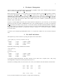
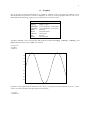
The plot command is the most generally used graphing command and l o g l o g , semilogx, semilogy, and
polar follow the same syntax as plot. For instance,
»a=0:0.1:10;
»b=sin(a);
»plot(a,b)
1
0.8
0.6
0.4
0.2
0
-0.2
-0.4
-0.6
-0.8
-1
0
1
2
3
4
5
6
7
8
9
10
produces a linear graph where the elements of the vector b are plotted versus the elements of vector a. Other
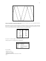
vectors can also be plotted on the same graph as shown below:
» c=cos(a);
» plot(a,b,a,c)
10
1
0.8
0.6
0.4
0.2
0
-0.2
-0.4
-0.6
-0.8
-1
0
1
2
3
4
5
6
7
8
9
10
If only one argument is used with the plot command then the elements of the vector are plotted versus their
respective matrix indices connected by a single line.
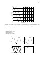
MATLAB also provides you with the flexibility of changing the line-type of your graphs to better distinguish
data from say, multiple experiments. Different colors can also be used but should be avoided unless you have
access to a color monitor or printer. The different line-types are summarized below:
Linestyle
point
circle
x-mark
plus
star
solid
dotted
dashdot
dashed
.
o
x
+
*
:
-.
--
y
m
c
r
g
b
w
k
Color
yellow
magenta
cyan
red
green
blue
white
black
The syntax is as follows: plot(vector1,vector2,’line-type’)
Labeling a graph is very simple and a list is found below:
title
xlabel
ylabel
text
gtext
grid
Labeling a Graph
graph title
x-axis label
y-axis label
arbitrarily positioned text
mouse-positioned text
grid lines
So, for example:
» plot(a,b,'*',a,c,'o')
» xlabel('x-axis in radians')
» ylabel('y-axis in radians')
» title('Graph of sin(a) in stars and cos(a) in circles')
» grid
11
Graph of sin(a) in stars and cos(a) in circles
1
0.8
0.6
y-axis in radians
0.4
0.2
0
-0.2
-0.4
-0.6
-0.8
-1
0
1
2
3
4
5
6
x-axis in radians
7
8
9
10
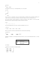
Frequently, it is convenient to show various plots on one sheet of paper. The command that divides the graph
screen into sub-windows is subplot. The syntax is as follows: subplot(mnr). Here, m is the number of
horizontal divisions (rows) and n is the number of vertical divisions (columns) of the graph screen. The r refers
to which window you want to plot the data. So take the following:
» subplot(221),plot(a,b)
» title('sin(a)')
» subplot(222),plot(a,c)
» title('cos(a)')
» subplot(223),plot(a,b,'*',a,c,'o')
» title('sin(a) and cos(a)')
» subplot(224),plot(a,log10(a))
» title('log10(a)')
sin(a)
cos(a)
1
1
0.5
0.5
0
0
-0.5
-0.5
-1
0
5
10
-1
0
sin(a) and cos(a)
1
0.5
0.5
0
0
-0.5
-0.5
0
5
10
log10(a)
1
-1
5
10
-1
0
5
10
12
Moreover, if you want to change the scale of the axes for a better presentation of the data simply type: axis([xmin x-max y-min y-max]). Here, x-min and x-max are the minimum and maximum values of your domain and ymin and y-max constitute your range.
Lastly, to print a graph simply choose F ile from the Figure Menu and click on P rint.... Click on the OK
button if the information presented on the Print Window is satisfactory.
9.
Environment Controls
The following is a brief list of the major interface controls available on MATLAB that have not been mentioned
previously:
who
whos
what
clc
clg
clear
clear variable
casesen
format
...
!
hold
delete
<Ctrl>-C
<Esc>
<Home>
<End>
Environment Commands
lists variables in memory
same as who with additional information
lists M-files in current directory
clears command screen
clears graphics screen
erases all variables from memory
erases variable from memory
toggles case sensitivity
changes numeric display on screen
indicates that statement continues on next line
executes operating system command
holds plot on screen
used to delete a file
local abort
deletes an entire input line
moves cursor to beginning of line
moves cursor to the end of the line
Please note that in the case of the format command, it might be easier to click on the Options menu item
then on N umeric Format to see what is available. Also, MATLAB is case sensitive so Z and z are two
different variables. By entering casesen you make MATLAB case insensitive where Z and z mean the same
thing.
10.
Polynomial Operations
Polynomials are represented by row vectors in MATLAB. For an nth order polynomial you need a row vector of
length n+1. For instance, if you want to express y=x3+5x-1 as a row vector then you would enter y=[1 0 5 -1].
Notice that the coefficients of the variable x are entered in the vector y so the “0” means that the term “x2” has
zero as a coefficient.
MATLAB is equipped with some very useful polynomial operations as listed below:
Polynomial Operations
roots
roots of a polynomial
poly
characteristic polynomial
polyval
polynomial evaluation
conv
polynomial multiplication
deconv
polynomial division
For example:
» r=roots(y)
r=
13
-0.0992 + 2.2427i
-0.0992 - 2.2427i
0.1984
» poly(r)
ans =
1.0000
0.0000
5.0000 -1.0000
» polyval(y,-2)
ans =
-19
In the above example, the roots of y have been calculated and stored in the column vector r. Furthermore, by
entering poly(r) the original coefficients of y were returned, as expected. Next, the polynomial was evaluated at
x=-2 by using the polyval function.
If you had a second polynomial w=2x2-x-1, then its corresponding row vector would be w=[2 -1 -1] and you
could enter the following:
» z=conv(w,y)
z=
2 -1 9
-7
» [Q,R]=deconv(z,w)
Q=
1 0 5 -1
R=
0 0 0 0
-4
1
0
0
Hence, the multiplication of w and y yields z=2x5-x4+9x3-7x2-4x+1 and dividing z by w yields the coefficients of
y with no remainders, as expected.
11.
System Models and Response
In the first half of the Dynamics of Systems course, emphasis will be placed on modeling and determining the
State-Space Model Equations. The second half will center around time and frequency response analysis.
MATLAB contains functions related to these two sections.
In the first section, MATLAB allows you to quickly find the transfer function of a State-Space Model and viceversa. Moreover, if the zeroes and poles of the transfer function are known then the transfer function or StateSpace Model can be found directly. These commands are summarized below with an example:
ss2tf
ss2zp
tf2ss
tf2zp
zp2tf
zp2ss
Model Conversions
state-space to transfer function
state-space to zero-pole
transfer function to state-space
transfer function to zero-pole
zero-pole to transfer function
zero-pole to state-space
Example: Find the State-Space Model of the transfer function G(s)=1/(s2+2s+1)
» num=[1];
» den=[1 2 1];
» [A,B,C,D]=tf2ss(num,den)
14
A=
-2
1
B=
1
0
C=
0
D=
0
-1
0
1
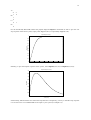
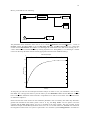
For the second half, MATLAB contains the popular step and impulse commands. In order to plot the unit
step response of the above system, simply enter step(num,den) or equivalently step(A,B,C,D):
Step Response of G(s)
1
0.9
0.8
0.7
Amplitude
0.6
0.5
0.4
0.3
0.2
0.1
0
0
2
4
6
8
Time (secs)
10
12
14
Similarly, to plot the impulse response of the system, enter impulse(num,den) or impulse(A,B,C,D):
Impulse Response of G(s)
0.4
0.35
0.3
Amplitude
0.25
0.2
0.15
0.1
0.05
0
0
0.5
1
1.5
2
2.5
3
Time (secs)
3.5
4
4.5
5
Unfortunately, MATLAB does not contain the ramp function. Consequently, one way to find the ramp response
is to use the Clock icon in SIMULINK as the input to your system (see Chapter 16).
15
A more general method of graphing the time response of a system for an arbitrary input is to use the l s i m
command. The syntax is as follows: lsim(num,den,u,t) or lsim(A,B,C,D,u,t). Here, u is the arbitrary input
vector and t is the time vector. Obviously, the input and time vectors must have the same dimensions.
In terms of frequency response, both magnitude and phase bode plots can be graphed by using the bode
command. For example, entering bode(num,den) yields:
Bode Plots of G(s)
Gain dB
0
-20
-40
-60 -1
10
0
1
10
Frequency (rad/sec)
10
Phase deg
0
-90
-180
-1
0
10
1
10
Frequency (rad/sec)
12.
10
Logical Operations
MATLAB is equipped with three logical operators, as shown below, that work elementwise on a matrix. For
the sake of Boolean Algebra, MATLAB considers anything with a non-zero real part as TRUE and returns the
value of “1” and everything else as FALSE and assigns the value of “0”.
Boolean
Operators
&
AN
|
D
~
OR
NOT
The & and | operators compare two scalars or two matrices of equal dimensions. The
example:
»v=[1 0 -3+i -4] & [-1 2 6 9]
v=
1 0 1 1
»v=[1 0 -3+i -4] | [-1 2 6 9]
v=
1 1 1 1
»~v
ans =
0
0
0
0
~
is a unary operator. For
16
Comparison of matrices can also be done with the familiar relational operators, as shown in the table, and
examples have been included below:
Relational Operators
<
less than
<=
less than or equal
>
greater than
>=
greater than or equal
==
equal
~
=
not equal
»v=[1 -1 2 -2] <= [4 -5 6 -7]
v=
1 0 1 0
»v=[1 -1 2 -2] > [4 -5 6 -7]
v=
0 1 0 1
Two functions which are frequently used with logical operators are any and all. By entering any(A), “1” will
be returned if the real part of any element of the vector A is non-zero. If A is a matrix then “1” will be returned
if the real part of any column entry of A is non-zero. The function all works in the same way as any only that
now all elements or column entries must have a real non-zero part for “1” to be returned.
13.
Control Flow
MATLAB has several control flow statements like those found in most computer languages which allows you
to write short programs. The FOR, WHILE, IF, and IF ELSE Control Loops will be described below with an
example.
FOR Loop
for v = expression
statements
end
Example
»for i=1:3
S(i)=i*(i+1)*(i+2);
T(i)=i/(i+1);
end
»S
S=
6 24 60
»T
T=
0.5000 0.6667 0.7500
WHILE Loop
while expression
statements
end
IF Loop
if expression
Example
»x=1;
»while x^3 <= 100
x=x+1;
end
»x
x=
5
Example
»d=5;
»if d>0
17
statements
e=sqrt(8);
end
»e
e=
2.8284
end
IF ELSE Loop
if expression
Example
»g=-2;
»if g>=0
statements
g=g^2;
else
else
g=abs(g);
end
»g
g=
2
statements
end
14.
Function M-Files
MATLAB allows you to create your own functions using M-Files. An M-File is an ordinary ASCII text file of
the form *.m which can be created using any text editor or word processor. The two categories of M-Files are
functions (this chapter) and scripts (Chapter 15).
The main advantage of having user-created functions is that they can be written to solve specific problems. It
must be kept in mind, however, that the basic difference between function and script M-Files is that the
arguments used in a function act locally and do not affect the workspace whereas variables defined in script MFiles act globally.
In order to write any M-File in the Windows Environment, simply click on N ew from the F ile menu and then
click on M-fi le. The Notepad Window will appear where you can start typing. When you have finished, save
the file on the hard-disk in your home directory and on a diskette. This is done by clicking on F ile then Save
A s . . . . Type the name of the file with the extension .m in the File N ame: input box. Make sure the
Driv es: selection box has f: emf/home:your login name when you are saving it to your directory and a:
when you are saving the file to a floppy diskette.
When creating a function M-File, the first line must begin with the word function and could have the general
form: function function-name(argument1, argument2, etc.). For example,
function y=witch(x)
%WITCH(X)
Draws the witch curve y=x^4-2x^2
y=x.^4-2*x.^2
%It’s the letter W!!!
is a function M-File called witch.m which can be called in the following manner:
»s=-2:0.01:2;
»t=witch(s);
»plot(s,t)
»title('The Witch Curve')
18
The Witch Curve
8
7
6
5
4
3
2
1
0
-1
-2
-1.5
-1
-0.5
0
0.5
1
1.5
2
Please note that the percent sign (%) denotes a comment and will be ignored by the MATLAB compiler. Also,
if you were to type help witch, you would only get the comments following the first line:
»help witch
WITCH(X)
Draws the witch curve y=x^4-2x^2
If you have to make a modification to your M-File or you want to retrieve it from your directory or floppy,
simply click on F ile then Open M-file.... Change the Driv es: box as required. Click on your M-File from
the list and click the OK box in order to get its window and revise it. When you finish, resave it by clicking on
F ile then S ave. In the Command Window you must type clear function-name before running your revised MFile since the old version is still in primary memory.
15.
Script M-Files
A script is simply an M-File with a list of MATLAB commands. When their name is entered in the Command
Window, the commands are executed in sequence and operate globally on the data in the workspace. Comments
can be added to a script for clarification purposes but not for the help command. The script sombrero.m was
written to draw the graphic on the cover page of this primer and is presented below:
x=-8:.5:8;
y=x;
[X,Y]=meshgrid(x,y);
R=sqrt(X.^2+Y.^2) + eps;
Z=sin(R)./R;
mesh(Z)
title('The Mexican "Sombrero"')
An equivalent but more tedious way of running a script M-File is to click on R un M - f i l e . . . from the F i l e
pull-down menu. In the input box entitled E nter M-file to run: type (disk location a: or f:)\name of script
M-file.m and click the OK box. If you do not recall the name of your M-File or you would rather choose from a
list, click on B rowse... then change the disk location in the Driv es: box. Select your file by clicking on it
then press the OK box twice.
Finally, since M-Files are regular text files, data can be stored within them and exported to other applications
such as Microsoft Excel for graphing purposes.
19
16.
SIMULINK
SIMULINK is a program within MATLAB that allows you to simulate dynamic systems modeled by block
diagram architecture. The blocks are supplied by SIMULINK in a block library which is organized into common
subsystems. By copying blocks from these subsystems into an unused window and connecting them,
simulations can be run and the corresponding data analyzed in MATLAB’s workplace. In order to describe the
syntax employed within SIMULINK for constructing block diagrams, a simple simulation of a first order
system will be performed.
Example: A research submarine is traveling underwater parallel to the ocean floor. Its effective mass while
submerged is M=2400kg. The drag coefficient B=320kg/s and the force of the propulsion system is a constant
F=1130N. Sketch the velocity v(t) of the submarine as a function of time if v(0)=0.
First of all, the physical model would be a mass M being pulled by a force F and retarded by a drag force Bv(t).
The governing equation can be found by drawing a Free Body Diagram of the submarine and using Newton’s
Second Law of Motion. Hence:
. B
F
v+
v=
M
M
To determine the velocity as a function of time, the above differential equation can be solved by first finding the
solution to the homogeneous equation then the particular solution. By adding these two solutions you get:
v(t ) =
Fæ
ç
Bè
- B tö
1- e M
÷
ø
The above equation can be used to plot the submarine’s velocity versus time in the MATLAB workplace but
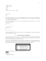
this would defeat the purpose of learning SIMULINK. Hence, enter simulink at the command prompt. A
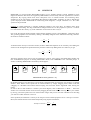
window containing SIMULINK’s block library should appear:
Sources
Sinks
Discrete
Linear
Nonlinear
Connections
Extras
SIMULINK Block Library (Version 1.2c)
By double-clicking on any subsystem, a list of blocks contained within the subsystem will appear in a separate
window. These blocks can be copied into an unused window by simply dragging them. Please note that
“dragging” in a Windows Environment means keeping the left mouse button suppressed while moving the
mouse.
In order to have a clean window to construct your block diagram, click on F ile then on N e w . . . . Move the
window to a convenient location on the screen by dragging the blue menu bar. If necessary, resize your window
by moving your mouse pointer near one of the window’s edges until you see it become a double arrow then drag
your mouse in either direction to resize it.
In this problem, the submarine’s velocity is the Output Variable and the propulsive force is the Input Variable.
Hence, the transfer function can be found analytically using Laplace Transforms,
Transfer Function =
v( s )
F(s)
=
1
Ms + B
20
and since F is a constant at t=0 seconds then we can say that it is a step input so:
F(s) =
F (t )
s
With this preliminary analysis complete, you can now begin your search for blocks that will help model the
system. Obviously, it takes time and practice to figure out which blocks to use and where to find them
depending on your system so one suggestion is to browse through the library and experiment with different
blocks. Double-click on the Sources subsystem block and drag the Step Fcn and Clock blocks to your window.
The Step Fcn block will help model the propulsion system and the Clock is needed to keep track of time, as
shown later on.
Step Fcn
Clock
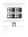
Now, close the Sources window and double-click on Sinks. Drag the Scope and To Workspace blocks into your
window then close Sinks. The Scope allows you to verify the output directly from SIMULINK and the To
Workspace block creates the default variable yout in the MATLAB workspace for analysis purposes.
Scope
yout
To Workspace
Finally, double-click on Linear and drag the Transfer Fcn block then close the Linear window. This block will
allow you to enter the transfer function derived above.
1
s+1
Transfer Fcn
Please note that it is imperative that unused windows be closed in order to save memory space for computational
purposes and graphics.
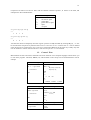
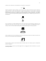
You are now ready to construct your block diagram. Start by dragging the blocks around until you get the
following orientation:
21
Step Fcn
1
s+1
yout
To Workspace
Transfer Fcn
Scope
Clock
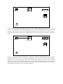
Next, connect the Step Fcn and Transfer Fcn blocks. This is done by dragging the angle bracket (>) out of
Step Fcn, representing the outport, to the angle bracket (>) into Transfer Fcn, representing the inport. Once the
connection is successful, a line with an arrowhead showing the direction of data flow and a little black square
signifying the fact that the arrow has been selected can be seen. Click anywhere in the window to unselect the
arrow:
Step Fcn
1
s+1
yout
To Workspace
Transfer Fcn
Scope
Clock
Proceed by connecting the Transfer Fcn and the To Workspace blocks in a similar fashion. Now, connect the
output of Transfer Fcn to Scope. This is done by selecting the arrow coming out of Transfer Fcn by clicking
anywhere on it. You should see a little black square. Drag the square along the arrow until you are halfway
towards To Workspace and release the mouse button. You should see an angle bracket on the arrow. Drag it
vertically down until you are level with the inport to the Scope and release the mouse button. Finally, drag the
angle bracket into the inport of Scope to finish the connection.
22
Step Fcn
1
s+1
yout
To Workspace
Transfer Fcn
Scope
Clock
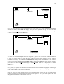
Next, copy the To Workspace block by first selecting it (i.e. just click on it to see a rectangle with four black
squares at its corners). Choose E dit then C opy. Move your mouse pointer to the right of Clock and click
once. Now, click on E dit then on P aste. You should have a To Workspace1 block on your window. Drag it
so that it is level with Clock and connect them.
Step Fcn
1
s+1
yout
To Workspace
Transfer Fcn
Scope
Clock
yout
To Workspace1
You must now change the default settings of the blocks to ensure that it corresponds with the submarine
system. Double-click on the Step Fcn block and change the Step time: to 0 and the Final value: to 1130
by using your mouse pointer to position the cursor on the input lines. Click on OK to close the window.
Double click on Transfer Fcn and change the Denominator: setting to [2400 320] and click on OK. Doubleclick on To Workspace and change the Variable name: to v then press OK. Double-click on Scope so that a
grid is shown and change the Horizontal range to 40 and V ertical Range to 4. Keep the Scope window
open so that you can observe the simulation. Double-click on To Workspace1 and change the Variable
name: to t.
Now, position your pointer over the title “To Workspace” and click once. It should be highlighted in blue. Type
“Velocity”. Similarly, change “To Workspace1” to “Time”. Note that once you finished typing, click anywhere
on the window so that the new title can center itself.
Lastly, the Transfer Fcn block should be hiding most of the denominator “2400s+320”. To correct this, select
the block by clicking once on it and drag one of the four corner squares out with your mouse pointer. This will
enlarge the block and allow the denominator to be seen.
23
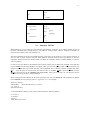
Hence, you should have the following:
1
2400s+320
Step Fcn
v
Velocity
Transfer Fcn
Scope
t
Time
Clock
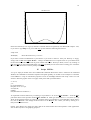
The parameters of the simulation must now be set so choose S imulation then Param eters.... Click on
Linsim, change the Stop Time: to 40, set Min Step Size: to 0, and Max Step Size: to 1.5 then click
on OK. Choose S imulation then S tart. You should get the characteristic first order curve leveling out at »
3.5m/s. Return to the Command Window by clicking anywhere on it. Enter plot(t,v). You should get a similar
curve as on the Scope Window as shown below (appropriate titles have been added for clarity):
Submarine Example
4
3.5
3
Velocity (m/s)
2.5
2
1.5
1
0.5
0
0
5
10
15
20
Time (s)
25
30
35
40
At this point, you can save the workspace for future analysis. In order to save your simulation, click on F i l e
then Save A s... and type the name of your file where you see untitled.m. Make sure the Driv es: selection
box is correct. The simulation will be saved as a script M-File so in order to run it follow the same instructions
as outlined in Chapter 15.
Please note that the values chosen for the simulation parameters were not arbitrary but rather they followed a
general rule of thumb for first order systems. That is to say, the Stop Time: was set equal to five time
constants and the Max Step Size: was set to one-fifth of the time constant. The time constant for the
submarine example is M divided by B which comes out to be 7.5 seconds. Moreover, Linsim was selected as
the integration routine since our system is quite linear. For non-linear systems Runge-Kutta 5 would be a
24
better choice. Needless to say, more complicated systems will need more time and experimentation to find the
best values for the simulation parameters so be patient and do not get discouraged.
* * * * *