Download s - Bison Academy

ECE 461 - Spring2010 - Page 1/3
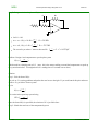
EE 461: Controls Systems I
http://venus.ece.ndsu.nodak.edu/~glower/ee461/index.html
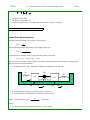
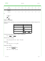
Instructor:
Office Location:
Office Phone:
Office Hours:
Class Hours:
Class Location:
Prof. Jake Glower
EE Building 101Q
231-8068
t.b.d.
MWF 3-4
FLC 313
Introduction:
Control systems is the study of dynamic systems and how to regulate the output of such systems.
Dynamic systems are any system which are described by differential equations. These include the voltage in an RLC circuit,
the temperature of a person, the flow of a fluid through a jet engine, the inflation rate in a country, etc. For all such systems,
the output responds to the input with a delay - a characteristic of a dynamic system. For all these systems, it is desirable to
adjust the input so that the output remains constant (such as body temperature at 98.6F regardless of external disturbances
such as wind or internal disturbances, such as exercise).
Control theory is the study of how to define the input so that the output behaves well.
In this class, 'classical control' theory is presented. This approach was developed in the U.S. and Europe from 1900 to 1950
for designing feedback amplifiers, anti-aircraft guns, and rockets. To this day, these approaches are the most commonly used
and serve as the foundation of subsequent control theory (such as Modern Control, developed in the U.S.S.R. in the 1950's,
digital control adaptive control, robust control, optimal control, etc.).
The heart of control theory is the study of differential equations (termed 'Applied Math' in the math department). Key to this
study is the se of LaPlace transforms - a mathematical tool which transforms differential equations into algebraic equations in
's'. Also of use are mathematical tools, such as MATLAB, which allow you so solve 10th-order algebraic equations or use
complex math with ease, or VISSIM, which allows you to simulate a differential equation with 'point and click' operations
rather than programming in a differential equation in C.
Requirements:
ECE 343: Signals and Systems is required for this course. It is assumed that the students have an understanding of LaPlace
transforms, solving differential equations using LaPlace transforms.
Good algebra skills are also useful, since the LaPlace transform will convert dynamic systems into sets of algebraic
equations.
A calculator which can do complex math is very useful for this course. A common problem in this class (and on tests will be
1000
⎞ evaluated at s = −2 + j4 .
to find the value of ⎛⎝ s(s+5)(s+20)
⎠
A calculator which solves for f(x)=0 is also very useful. A common problem will be to solve for 'a' so that
1000
⎞ = −140 0 evaluated along the line s = a∠90 0 . Graphical techniques can and will be used on tests and
angle ⎛⎝ s(s+5)9s+20)
⎠
homework. Numerical solutions are much easier to find if your calculator can do this (MATLAB can solve such problems
but is not available on tests).
Text Book:
A text book is required for this course. Each student is expected to find or borrow copy for the semester. Note that new
control theory text books cost between $150 and $250 per copy. Instead of buying a new text, however, I'd suggest finding
an older copy from
ECE 461 - Spring2010 - Page 2/3
www.amazon.com (29,000 hits for "feedback control theory)
overture.directtextbook.com/textbooks/173515_Engineering
www.half.com
www.ebay.com
Grading
Midterms:
Homework & Quizzes
Final
Total:
1 unit each
1 unit
1 units
Average of all above
Final Percentage:
100% - 90%
89% - 80%
79% - 70%
69% - 60%
< 59% E
A
B
C
D
Grading will be on a straight scale to encourage working together. My objective is to see that everyone learns the material.
If the class studies together and everyone gets a 90% average, I'd gladly give all A's. (After all, your competitors are at
schools like UCLA, Michigan, etc. - they're not your classmates.)
Policies:
A student may take a makeup exam if he/she misses an exam due to an emergency, illness, or plant trip and notifies me in
advance of the exam. Late homework will not be accepted once the solutions are posted online. All questions on the grading
of a particular exam must be resolved within a week of returning the exam.
Quizzes: Each Friday, there will be a short 15 minute quiz. The topics cover what we're doing in class or the prerequisites
of ECE 461 (namely calculus, circuits, and signals and systems). The quizzes are closed book, closed note, no calculator.
Topics that are fair game for any quiz are:
ECE 343:
Fourier Transforms: Be able to determine the spectral content of a square wave, etc.
LaPlace Transforms: Be able to find the inverse LaPlace transform of ⎛⎝ s(s+10) ⎞⎠ or similar
20
Z transform: Be able to find the inverse z-transform of ⎛⎝ z(z+10) ⎞⎠
20
ECE 311:
Find the transfer function of an op-amp circuit with resistors, inductors, and capacitors
Design a circuit with a gain of +10 or -10.
Homework: Homework is graded as
80%: You attempted the problem with an organized approach I can follow.
20%: You got the right answer.
Homework is practice using the tools being presented. Copying someone else's homework is sort of like watching someone
else exercise. You need to do it yourself. Similarly, with grading I care most that you attempted the problem and thought
about it.
Labs: Labs are a part of the homework sets (For example, problems 7-10 might be finding the transfer function for a motor
you'll find in the lab.) To get credit for those homework problems, you have to attend lab.
ECE 461 - Spring2010 - Page 3/3
Testing: All tests will be closed-book, closed-notes, open calculator. Midterms serve to identify who put in the time solving
the homework problems. My goal in writing tests is add new twists you havn't seen yet so that
If you did the homework and are comfortable with the concepts and tools, you'll have a shot at the midterms.
If you copied someone else's homework, you'll be lost.
The best way to study for the midterm is to make up your own midterm. There's only so many ways to ask a question.
Special Needs - Any students with disabilities or other special needs, who need special accommodations in this course are
invited to share these concerns or requests with the instructor as soon as possible.
Academic Honesty - All work in this course must be completed in a manner consistent with NDSU University Senate
Policy, Section 335: Code of Academic Responsibility and Conduct. Violation of this policy will result in receipt of a failing
grade.
ECE Honor Code: On my honor I will not give nor receive unauthorized assistance in completing assignments and work
submitted for review or assessment. Furthermore, I understand the requirements in the College of Engineering and
Architecture Honor System and accept the responsibility I have to complete all my work with complete integrity.
NDSU
1.03: LaPlace Transforms and First and Second Order Approximations
ECE 461
LaPlace Transforms
Assumption:
LaPlace transforms assume all functions are in the form of
⎧ a ⋅ e st
y(t) = ⎨
⎩ 0
t>0
otherwise
This results in the derivative of y being:
dy
dt
= s ⋅ y(t)
Tables for LaPlace Transforms:
You can think of 's' as an operator meaning 'the derivative of'. Initial conditions also come into play as follows:
Table 1: LaPlace Transforms with Initial Conditions
Time: y(t)
LaPlace: Y(s)
y
Y
y'
sY - y(0)
2
y''
s Y - y'(0) - sy(0)
From ECE 343, several common functions have the following LaPlace transform:
Table 2: Common LaPlace Transforms
Name
delta (impulse)
unit step
Time: y(t)
LaPlace: Y(s)
δ(t)
1
1
s
a
s+b
u(t)
a ⋅ e −bt u(t)
2a ⋅ e −bt cos(ct − θ)u(t)
⎛ a∠θ ⎞ + ⎛ a∠−θ ⎞
⎝ s+b+jc ⎠ ⎝ s+b−jc ⎠
Example:
Find the output of a system which satisfies the following differential equation:
y'' + 3'y + 2y = 4u
given that all initial conditions are zero and u is a unit step input.
Solution:
Convert to LaPlace notation
JSG
1
rev August 21, 2007
NDSU
1.03: LaPlace Transforms and First and Second Order Approximations
ECE 461
s 2 + 3s + 2)Y = 4U
Substitute for U
1
(s 2 + 3s + 2)Y = 4 ⎛⎝ s ⎞⎠
Solve for Y
Y=
4
s(s 2 +3s+2)
=
4
s(s+1)(s+2)
Use partial fraction expansion
−4 ⎞
⎛ 2 ⎞
Y = ⎛⎝ 2s ⎞⎠ + ⎛⎝ s+1
⎠ + ⎝ s+2 ⎠
And convert back to time using Table 2.
y(t) = (2 − 4e −t + 2e −2t )u(t)
Example 2:
Find the y(t) given that
15
⎞ ⋅ ⎛1⎞
Y(s) = G ⋅ U = ⎛⎝ s 2 +2s+10
⎠ ⎝s⎠
Solution:
Factoring Y(s)
15
⎞
Y(s) = ⎛⎝ (s)(s+1+j3)(s+1−j3)
⎠
Using partial fraction expansion:
⎞ ⎛ 0.7906∠−161.56 0 ⎞ + ⎛ 0.7906∠161.56 0 ⎞
Y(s) = ⎛⎝ 1.5
s ⎠ +⎝
s+1+j3
⎠ ⎝ s+1−j3 ⎠
y(t) = 1.5 + 1.5812 ⋅ e −t ⋅ cos (3t + 161.56 0 )
for t>0
note: Control systems is actually easier than signals and systems. In controls, we limit ourselves to one
dimensional causal systems (time is one dimensional and only moves forward). For motors, lights, etc. this is a
physical limitation. (if you could build a system where the output happens before the input, you can make lots of
money in Las Vegas.)
In Signals and Systems, you can have non-causal systems. For example, if you are filtering an image, you can
filter left to right, right to left, or even up and down. Signals and Systems likewise uses mathematics that work
for multiple non-causal dimensions.
JSG
2
rev August 21, 2007
NDSU
1.03: LaPlace Transforms and First and Second Order Approximations
ECE 461
First and Second Order Approximations
Objectives:
In this section we will look at
Determining the dominant poles of a system
Be able to time-scale a system
Simplifying a transfer function by replacing it with a first or second-order approximations
Predicting a system's behavior based upon this first or second order approximation
Definitions:
Dominant Pole(s): The pole which dominates the step response of a system. These are the poles which are
closest to the jw axis.
G(s):
The transfer function of a system
DC Gain:
G(s) at s=0. The gain of a system for a constant input.
Settling Time: The time it takes the transients to decay to 2% of their initial value
Overshoot: The maximum of a step response divided by it's steady-state value.
Step Response: The output of a system when a unit step is applied to the input (U(s) = 1/s)
Resonance: The maximum gain vs. frequency, normalized by the DC gain.
Damping Ratio: The cosine of the angle of a complex pole as measured from the negative real axis.
Dominant Pole:
A transfer function represents a differential equation which models the response of a dynamic system. The
purpose of using transfer functions is to simplify analysis while accurately describing a system's response. The
complexity of a transfer function represents two conflicting goals:
More complex transfer functions (i.e. more poles and zeros) are better able to model a system's response
Simpler transfer functions are easier to understand and use for analysis.
When extremely accurate models are required, the system can be very high order. The Maverick Missile, for
example, was modeled as a 250th order differential equation. Often times, a crude model will suffice. In this
case, a simple model which captures the overall behavior of a system will do.
In order to obtain this simple model, the transfer function needs to be
Simplified (reducing the order and complexity of the model), and
Accurate, still capturing the system's overall behavior.
In short, you want to simplify the transfer function to one which includes the poles which dominate the system's
response.
If a system has several poles, these dominant poles will be the ones which
Have the largest initial condition (i.e. most energy), and
Slowest decay rate (so they last the longest).
JSG
3
rev August 21, 2007
NDSU
1.03: LaPlace Transforms and First and Second Order Approximations
ECE 461
It turns out that the pole(s) closest to s=0 has the largest initial condition and the pole(s) closest to the jw axis
have the slowest decay rate. Often the same pole satisfies both of these conditions.
Example: Find the dominant poles of
2000
⎞
G(s) = ⎛⎝ (s+1)(s+10)(s+100)
⎠
Solution: The step response of this system is
2000
⎞ ⎛1⎞
Y(s) = ⎛⎝ (s+1)(s+10)(s+100)
⎠⎝s⎠
Using partial fraction expansion
⎞ + ⎛ 0.2469 ⎞ + ⎛ 0.0022 ⎞
Y(s) = ⎛⎝ 2s ⎞⎠ + ⎛⎝ −2.222
s+1 ⎠
⎝ s+10 ⎠ ⎝ s+100 ⎠
The step response is then
y(t) = (2 − 2.222e −t + 0.2469e −10t − 0.0022e −100t )u(t)
Note that
The first term (2) is the forced response. It remains as long as the input remains equal to 1.
The second term (-2.22e-t) has an initial condition 9x larger than any other term and it decays slower than
the other terms.
Hence, the pole at s=-1 dominates the response (and is termed the dominant pole).
Once the dominant pole has been identified, you can simplify the transfer function by
Keeping the dominant pole(s), and
Keeping the DC gain unchanged.
(DC is often used since most control systems are to track constant or slowly changing inputs, such as the desired
temperature in a room, flow through a pipe, etc.)
Example: Find a simplified model for G(s) from above.
Solution: Since the dominant pole is at -1
2000
⎞ ≈⎛ a ⎞
G(s) = ⎛⎝ (s+1)(s+10)(s+100)
⎠ ⎝ s+1 ⎠
The constant 'a' is selected so that G(s=0) is the same in both cases. Setting the DC gain to be the same
2 ⎞
G(s) ≈ ⎛⎝ s+1
⎠
Example: Find a simplified model for a system with complex poles:
2000
⎞
G(s) = ⎛⎝ (s+1+j2)(s+1−j2)(s+10)(s+50+j200)(s+50−j200)
⎠
Solution: The dominant pole is the pole which decays the slowest and is closest to s=0 are (-1+j2, -1-j2). Since
the pole is complex, its complex conjugate will also be present in any model. Both decay at the same rate, so
there are two dominant poles.
JSG
4
rev August 21, 2007
NDSU
1.03: LaPlace Transforms and First and Second Order Approximations
ECE 461
The simplified model is then
2000
a
⎞ ≈⎛
⎞
G(s) = ⎛⎝ (s+1+j2)(s+1−j2)(s+10)(s+50+j200)(s+50−j200)
⎠ ⎝ (s+1+j2)(s+1−j2) ⎠
Setting the DC gain to be the same, 'a' is found to be 0.000941
0.000941
⎞
G(s) ≈ ⎛⎝ (s+1+j2)(s+1−j2)
⎠
Time Scaling
Since a transfer function is only a model that simulates a real system, it is not necessary for one second in
simulation time to correspond to one second in real time. Sometimes, it is an advantage to have different time
scales. For example, if modeling the effect of interest rates on the U.S. economy, it would be very convenient if 1
month real time corresponded to 1 second in simulation time. Events which take effect in 6 months could then be
observed in 6 seconds. Fast events can also be slowed down so that you can observe what is going on (such as
modeling the propagation of a flame or pressure wave).
In order to time scale a transfer function
i) Define the relationship between simulation time (τ ) and real time (t) as τ = αt .
For example, if 1s simulation time corresponds to 1ms real time (i.e. the simulation is 1000x slower than
the actual system), τ = 0.001t .
ii) Substitute for s → αs
The LaPlace transform assumes all functions are in the form of e st . Substituting for t results in all
functions being in the form of e (s/α)τ .
s
To slow up the system by 1000, replace s with 0.001
= 1000s .
iii) Simplify the transfer function.
10 7
⎞ . Find the transfer function if time
Example: The dynamics of a servo-motor are given as G(s) = ⎛⎝ s(s+500)(s+2000)
⎠
scaled by 1000x (i.e. the model is 1000x slower than the actual system.)
Solution: Replace 's' with 1000s
10 7
⎞ = ⎛ 0.01 ⎞
G(s) ⇒ ⎛⎝ (1000s)(1000s+500)(1000s+2000)
⎠ ⎝ s(s+0.5)(s+2) ⎠
note: In this course, most systems will have poles with a magnitude close 1. This is done since i) with time
scaling, any system can be modeled as one with poles close to 1, and ii) 1 has nice numerical properties. (i.e.
1n=1)
First-Order Approximations:
JSG
5
rev August 21, 2007
NDSU
1.03: LaPlace Transforms and First and Second Order Approximations
ECE 461
Assume the simplified model for a system is a first-order system. Given this model, try to predict how the system
will behave, including
The steady-state gain (if an input of 1 is applied, what will the output go to?)
The settling time (how long it takes to reach steady-state), and
The bandwidth (if the input is a sinusoid, what frequency range will be passed?)
Consider a generic 1st-order system
a ⎞
G(s) = ⎛⎝ s+b
⎠
The DC gain is G(s=0), or a/b
The steady-state gain is G(s=0) = a/b
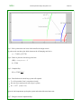
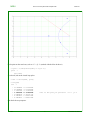
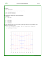
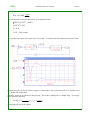
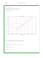
1 ⎞ ⎛ 2 ⎞ ⎛ 3 ⎞
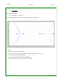
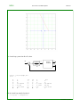
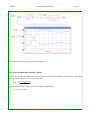
Example: Plot the step response of ⎛⎝ s+1
⎠ , ⎝ s+1 ⎠ , ⎝ s+1 ⎠
Solution: From MATLAB:
»
»
»
»
»
»
»
G2 = tf(2,[1,1]);
G3 = tf(3,[1,1]);
t = [0:0.1:10]';
y1 = step(G1,t);
y2 = step(G2,t);
y3 = step(G3,t);
plot(t,y1,t,y2,t,y3)
Y
a/b=3
3
a/b=2
2
a/b=1
1
0
0
1
2
3
4
5
Seconds
6
7
8
9
10
Settling Time: The transient decays as e-bt. This transient decays to 2% of its initial value in
0.02 = e −bt
ln(0.02) = −3.912 = −bt
t=
3.912
b
seconds
or, since the model is only approximate anyway, this is usually defined as
t≈
4
b
The 2% settling time will be (approximately)
JSG
6
4
b
rev August 21, 2007
NDSU
1.03: LaPlace Transforms and First and Second Order Approximations
ECE 461
Another way to look at this is to use time scaling. If you slow down the simulation by a factor of 'b', the transfer
function becomes
a ⎞
⎛ a/b ⎞
G(s) ⇒ ⎛⎝ bs+b
⎠ = ⎝ s+1 ⎠
A system with a pole at -1 has a 2% settling time of about 4 seconds. Since this is a time-scaled system, the actual
system will have a settling time of 4b seconds.
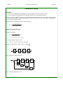
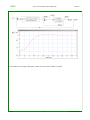
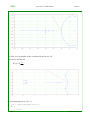
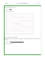
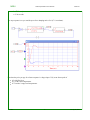
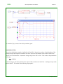
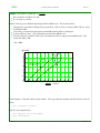
1 ⎞ ⎛ 2 ⎞ ⎛ 4 ⎞
Example: Plot the step response of ⎛⎝ s+1
⎠ , ⎝ s+2 ⎠ , ⎝ s+4 ⎠
from MATLAB:
Y
2% settling time for b=4
2% settling time for b=2
1
b=4
2% settling time for b=1
b=2
b=1
0
0
1
2
3
4
5
Seconds
The frequency response of G(s) is found by letting s=jw. The gain vs. frequency is then
a ⎞
G(jω) = ⎛⎝ jω+b
⎠
which is plotted below.
Normalized Gain (x a/b)
1
0.7
0.5
Gain is down 3dB at b rad/sec
0.3
0.2
0.1
0.1b
0.2b
0.3b
0.5b
b
rad/sec
2b
3b
5b
10b
At a frequency of b rad/sec, this gain drops to
JSG
7
rev August 21, 2007
NDSU
1.03: LaPlace Transforms and First and Second Order Approximations
G(jb) =
ECE 461
= ⎛⎝ a/b ⎞⎠
2
a
jb+b
or
The gain is down 3dB
The power is down 6db (1/2)
Frequencies past 'b' rad/sec are attenuated. Those below 'b' rad/sec are passed.
The bandwidth of the system is b rad/sec
Second-Order Approximations:
Assume the simplified model for a system is second-order:
ac ⎞
G(s) = ⎛⎝ s 2 +bs+c
⎠
Factoring the denominator and placing it in rectangular form gives
aω2n
⎞
G(s) = ⎛⎝ (s+σ+jωd )(s+σ−jω
d) ⎠
If you take the step response of this system, the terms will be of the form
y(t) = a + be −σt cos (ωd t + φ)
(t>0)
where 'b' and φ are constants. Note that the step response can be determined by inspection by looking at the
different terms in the transfer function:
a: Determines the DC gain. Doubling 'a' doubles the amplitude of the response.
K1
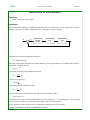
B3
m1
K3
m2
K2
f
B1
x1
B2
x2
ωd : Determines the frequency which the system oscillates at.
σ : Determines the rate at which the exponential envelope decays.
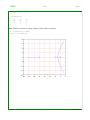
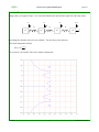
200
⎞
Example: Determine how G(s) = ⎛⎝ (s+2+j20)(s+2−j20)
⎠
will behave:
Solution:
The step response will eventually go to 0.495. (G(0) = 0.495).
JSG
8
rev August 21, 2007
NDSU
1.03: LaPlace Transforms and First and Second Order Approximations
ECE 461
It will take approximately 2 seconds to reach steady-state. (The real part of the dominant pole is -2.
Hence, the transient decays as e −2t ), and
The transient will oscillate at 20 rad/sec (the complex part of the pole is j20).
The actual step response follows:
Y
1
Exponential Envelope Decays as exp(-2t)
DC Gain = 0.495
0.5
2% Settling Time
20 rad/sec oscillations
0
2% Settling time =
0
1
2
Seconds
3
4
4
σ
Frequency of Oscillation = ω d
Resonance Frequency ≈ ω d
Often times, the overshoot in the step response if of interest rather than the frequency of oscillation. This is
easiest to predict if you express the transfer function in polar form:
aω2n
⎞
G(s) = ⎛⎝ (s+ωn ∠θ)(s+ω
n ∠−θ) ⎠
or
aω2
G(s) = ⎛⎝ s 2 +2ζωnns+ω2 ⎞⎠
n
where ζ = cos θ . If you time scale by a factor of ωn , and scale by the DC gain (a), this system becomes
1
⎞ =⎛ 1 ⎞
G(s) = ⎛⎝ (s+1∠θ)(s+1∠−θ)
⎠ ⎝ s 2 +2ζs+1 ⎠
From this, it is clear that
'a' determines the amplitude of the response (double 'a' and you double the output)
ωn (the amplitude of the poles) determines the speed of the system (i.e. the time scaling). Double ωn and
you halve the response time or double the bandwidth. (If you respond to higher frequencies, you respond
more quickly).
The 'shape' of the step or frequency response is determined by the angle of the complex poles (θ or the
damping ratio ζ )
This 'shape' determines the overshoot for a step response or amplitude of the resonance for a frequency response.
This is summarized on the second-order approximations sheet. Two commonly used terms are
JSG
9
rev August 21, 2007
NDSU
1.03: LaPlace Transforms and First and Second Order Approximations
ECE 461
−πζ
Overshoot =
e
1−ζ 2
⎧⎪
Resonance = Mm = ⎨
⎪⎩
ζ < 0.7
1
2ζ 1−ζ 2
ζ > 0.7
1
(If the damping ratio is greater than 0.7, there is no resonance and Mm does not apply)
Note: Since a complex pole only has two degrees of freedom, there is some redundancy here:
Real part of the pole (σ ) determines the settling time
Imaginary part of the pole (ωd ) determines the frequency of oscillation
Angle of the pole (θ or cos θ = ζ ) determines the overshoot and resonance,
The magnitude of the pole (ωn ) , determines the corner frequency on a Bode plot.
These are all related by through trigonometry as shown in the following figure. Hence, if you are going to specify
how a system should behave, you should only include two of the following requirements to avoid inconsistency:
Settling Time
Frequency of Oscillation (or resonance)
% Overshoot (if the magnitude of the resonance was not specified)
Magnitude of the Resonance (if % overshoot was not specified)
Corner frequency (bandwidth)
The type of system often determines which parameters are relevant. (For example, for an amplifier, resonance
and bandwidth are important. For a jet engine, settling time and overshoot are important.)
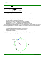
Imag
Wd
s-plane
Wn
Dominant Poles
Wn
Wd
Real
JSG
10
rev August 21, 2007
NDSU
1.03: LaPlace Transforms and First and Second Order Approximations
ECE 461
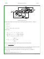
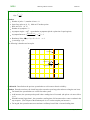
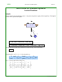
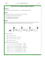
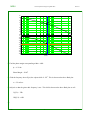
Example: Determine how mass x1 will behave when a step input is applied at F. Assume M=1, B=2, K=3.
Solution: From before, the transfer function is
2 +4s+6
⎞
x 1 = ⎛⎝ s 4 +8s 3s+24s
2 +36s+27 ⎠ F
Factoring
s 2 +4s+6
⎞F
x 1 = ⎛⎝ (s+1+j1.412)(s+1−j1.412)(s+3)(s+3)
⎠
The DC gain is 6/27. Mass x1 will eventually move 6/27 meter to the right.
The 'dominant' pole is at -1 + j1.412. The transient will take about 4 seconds. (σ = 1) The overshoot will be about
10.8% ( ζ = 0.578) . The actual step response is shown below. The actual response is a little different from what
the second order approximations would suggest since i) this system is actually 4th order, ii) the fast poles aren't
that much faster than the dominant poles, and iii) there are zeros in this system. In spite of this, the 2nd-order
approximations predict the step response fairly accurately.
X1
0.3
Steady State = 0.2222
0.2
7.87% Overshoot
Ts = 4 sec
0.1
0
0
1
2
3
4
5
6
7
Seconds
JSG
11
rev August 21, 2007
NDSU
102:: Block Diagrams & VisSim
ECE 461
Block Diagrams & VisSim
Objective:
Introduce block diagram notation
Be able to write the equations that describe a block diagram
Be able to simplify a block diagram
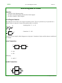
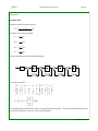
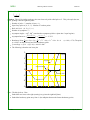
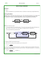
Block Diagram Notation
Block diagrams are one of the core concepts in controls systems. They are a pictorial way to represent how a
feedback system is connected. Some of the symbols used are as follows:
B
X
Summing block. Y = A - B
Y
A
-
Gain block: Y = GX
Y
G
With these, you can simplify a block diagram to a single gain. Sometimes it helps to add in dummy variables and
then simplify.
Series Connection:
U
K
X
G
Y
Y = GX
X = KU
simplifying:
Y = GK ⋅ U
Parallel Connection:
G
Y
U
K
JSG
1
rev August 17, 2009
NDSU
102:: Block Diagrams & VisSim
ECE 461
Y=G⋅U+K⋅U
Y = (G + K) ⋅ U
Feedback Configuration:
R
E
K
Y
G
H
Add in a dummy variable, E:
Y = (G ⋅ K) ⋅ E
E=R−H⋅Y
Simplifying:
GK ⎞
Y = ⎛⎝ 1+GKH
⎠R
Memorize this one. We'll be using it a lot this semester.
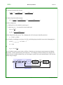
Feedback + Feedforward:
F
U
E
-
A
K
Y
G
H
Add in two dummy variables, E and A, to simplify the equations:
Y = GA
A = KE + FU
E = U − HY
Substitute and solve:
JSG
2
rev August 17, 2009
NDSU
102:: Block Diagrams & VisSim
ECE 461
Y = G(K(U − HY) + FU)
(1 + GKH)Y = (GK + GF)U
G(K+F)
Y = ⎛⎝ 1+GKH ⎞⎠ U
VisSim:
VisSim is a program from Visual Solutions Incorporated - designed specifically for the design, analysis, and
simulation of dynamic systems (i.e. ECE 461). It's similar to SciLab, but VisSim came first and I prefer it. Plus,
VisSim has a free departmental license (from http://www.vissim.com/products/academic.html):
A one year license to operate the software on an unlimited number of machines in the department. The free
license for the VisSim Academic Package will be renewed at no charge simply by registering for a license
extension at the termination of the first year license.
One user manual for each licensed product.
All department faculty members and students enrolled in the VisSim training program may make copies of the
software for personal use on- or off-campus.
Technical support is available to faculty members only..
Note:
You may use VisSim on a personal machine for one year.
You may use VisSim at NDSU for one year,
It's free for the year (!)
If you like the product, you can buy your own version for about $50.
Help manuals are located at
www.VisSim.com
VisSim Menu's
VisSim implements block diagrams used in controls systems. I've found it's very easy to use and intuitive. I've
never read the user manual and have had no problem. Pretty much, use the pull down menus to find stuff that
looks useful. This will illustrate some of the features we'll use in ECE 461.
Edit:
Flip Horizontal: Flip a block left to right. It sometimes makes a screen prettier if the input is on the right.
Create Compound Block: Highlight part of the screen and click on this. All the mess you highlighted is
placed inside a block. This cleans up the screen display. If you double-click on the block, you see what's
inside.
Add / Remove Connector: Add or remove inputs and outputs to compound blocks and summing junctions.
JSG
3
rev August 17, 2009
NDSU
102:: Block Diagrams & VisSim
ECE 461
Simulate: This lets you change how the program runs.
Simulation Properties lets you change the step size (0.001 or smaller usually). Integration Method is what form of
numerical integration is used. Usually use Runge Kutta 4th order or 5th order.
JSG
4
rev August 17, 2009
NDSU
102:: Block Diagrams & VisSim
ECE 461
Block: Pretty much everything you're going to use. Just scroll down each item until you find something that
sounds close. We'll go through some examples of more commonly used blocks.
Simulation in VisSim
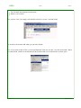
Example 1. Find the step response for the following system:
For this, we need
A transfer function, (menu Block, Linear System, Transfer Function)
A step input, (Block, Signal Producer, Step)
A summing junction (Block, Arithmetic, Summing Junction)
Add a transfer function. To input the one on the right, the numerator and denominator polynomials are input in
decreasing powers of s:
numerator = 1000
denominator = 1 25 100 0
JSG
5
rev August 17, 2009
NDSU
102:: Block Diagrams & VisSim
ECE 461
Once you add the blocks, connect them with arrows. (left click on the output of one block, left click on what it
connects to, repeat).
Set up the simulation to go from 0 to 2 seconds with a step size of 0.001 second.
Click on the green arrow to run the simulation.
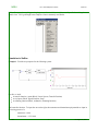
Example 2: Add Gaussian noise (N(0, 0.1)) to the measured output to simulate sensor noise. Also plot the input
to the last block:
Solution: Add Gaussian noise (Block, Random, Gaussian). Left click to change the block's parameters to mean 0,
standard deviation 0.1.
Add a variable to pretty up the screen. (Block, Annotation, Variable). Call these variables Y and U (output and
input).
Add a summing junction to add the real output to the noise to model the sensor.
JSG
6
rev August 17, 2009
NDSU
State Space & Canonical Forms
ECE 461
State-Space Representation of System Dynamics
State-Space is a matrix-based formulation for a system's dynamics. The standard form for the dynamics of a
linear system are
sX = AX + BU
Y = CX + DU
where Y is the system's output, U is the system's input, and X are 'dummy' states (termed internal states.) With
this formulation, the transfer function will be
X = (sI − A) −1 BU
Y = ⎛⎝ C(sI − A) −1 B + D ⎞⎠ U
MATLAB is a matrix language which has functions that let you find the transfer function of a system in
state-space form. It's much easier (and less prone to errors) if you express many systems in state-space form and
let MATLAB determine the transfer function. It's also an easier way to implement a system on a microcomputer.
MATLAB Commands
G = ss(A, B, C, D);
G = tf(num, den)
G = zpk(z, p, k)
ss(G)
tf(G)
zpk(G)
input a system in state-space form
input a system in transfer function form
input a system in zeros, poles, gain form
determine A, B, C, D for system G (answer is not unique)
determine the transfer function of system G
determine the zeros, poles, and gain of system G
Matrix Algebra
An nxm matrix has n rows and m columns. For example, a 2x3 matrix has 6 elements:
⎡a a a ⎤
A 2x3 = ⎢ 11 12 13 ⎥
⎣ a 21 a 22 a 23 ⎦
Scalar Multiplication:
⎡ ba 11 ba 12 ba 13 ⎤
bA = ⎢
⎥
⎣ ba 21 ba 22 ba 23 ⎦
Matrix Addition:
Matrices with the same dimensions can be added:
⎡ a a a ⎤ ⎡ b b b ⎤ ⎡ a + b 11 a 12 + b 12 a 13 + a 13 ⎤
A + B = ⎢ 11 12 13 ⎥ + ⎢ 11 12 13 ⎥ = ⎢ 11
⎥
⎣ a 21 a 22 a 23 ⎦ ⎣ b 21 b 22 b 23 ⎦ ⎣ a 21 + b 21 a 22 + b 22 a 23 + b 23 ⎦
Matrix Multiplication:
JSG
1
rev August 17, 2009
NDSU
State Space & Canonical Forms
ECE 461
To multiply two matrices, the inner dimensions must match
A xy ⋅ B yz = C xz
⎡b b
⎡ a 11 a 12 a 13 ⎤ ⎢ 11 12
⎢
⎥ ⎢ b 21 b 22
⎣ a 21 a 22 a 23 ⎦ ⎢ b b
⎣ 31 32
⎤
⎥ ⎡ a 11 b 11 + a 12 b 21 + a 13 b 31 a 11 b 12 + a 12 b 22 + a 13 b 32 ⎤
⎥=⎢
⎥
⎥ ⎣ a 21 b 11 + a 22 b 21 + a 23 b 31 a 21 b 12 + a 22 b 22 + a 23 b 32 ⎦
⎦
⎡ Σ a 1x b x1 Σ a 1x b x2 ⎤
=⎢
⎥
⎣ Σ a 2x b x1 Σ a 2x b x2 ⎦
Matrix Inversion
A⋅A
−1
⎡1 0 0 ⎤
⎥
⎢
=I=⎢ 0 1 0 ⎥
⎥
⎢
⎣0 0 1 ⎦
I = the identity matrix = the matrix version of '1'
For a 2x2 matrix,
⎡
A −1 = ⎢
⎣
a 22
Δ
−a 21
Δ
−a 12
Δ
a 11
Δ
⎤
⎥
⎦
Δ = a 11 a 22 − a 12 a 22
Placing a System in State-Space Form:
i) Write N equations for the N voltage nodes
ii) Solve for the highest derivative for each equation
iii) Rewrite in matrix form.
Example. The following differential equation describe the water level in a two-tank system. Write this in
state-space form and find the transfer function from U to Y.
dx 1
dt
= x 2 − x 1 + 0.3u
dx 2
dt
= x 1 − 1.3x 2
Write this as
sX = AX + BU
⎡ x ⎤ ⎡ −1 1 ⎤ ⎡ x 1 ⎤ ⎡ 0.3 ⎤
s⎢ 1 ⎥ = ⎢
⎥+⎢
⎥⎢
⎥U
⎣ x 2 ⎦ ⎣ 1 −1.3 ⎦ ⎣ x 2 ⎦ ⎣ 0 ⎦
If x2 is the output,
JSG
2
rev August 17, 2009
NDSU
State Space & Canonical Forms
ECE 461
⎡x ⎤
Y = ⎡⎣ 0 1 ⎤⎦ ⎢ 1 ⎥ + [0]U
⎣ x2 ⎦
To find the transfer function in MATLAB,
A
B
C
D
=
=
=
=
[-1, 1; 1, -1.3]
[0.3; 0]
[0, 1]
0;
G = ss(A, B, C, D)
tf(G)
Transfer function:
0.3
----------------s^2 + 2.3 s + 0.3
Example: The temperature along the length of a metal bar are described by
sx 1 = u − 2x 1 + x 2
sx 2 = x 1 − 2x 2 + x 3
sx 3 = x 2 − 2x 3 + x 2
sx 4 = x 3 − x 4
Find the transfer function from U to X4.
Solution: Express this in state-space form
⎡
⎢
s ⎢⎢
⎢
⎢
⎣
x1
x2
x3
x4
⎤ ⎡ −2
⎥ ⎢ 1
⎥=⎢
⎥ ⎢
⎥ ⎢ 0
⎥ ⎢
⎦ ⎣ 0
1
−2
1
0
⎡
⎢
y = ⎡⎣ 0 0 0 1 ⎤⎦ ⎢⎢
⎢
⎢
⎣
0
1
−2
1
x1
x2
x3
x4
0
0
1
−1
⎤⎡
⎥⎢
⎥⎢
⎥⎢
⎥⎢
⎥⎢
⎦⎣
x1
x2
x3
x4
⎤ ⎡
⎥ ⎢
⎥+⎢
⎥ ⎢
⎥ ⎢
⎥ ⎢
⎦ ⎣
1
0
0
0
⎤
⎥
⎥U
⎥
⎥
⎥
⎦
⎤
⎥
⎥ + [0]U
⎥
⎥
⎥
⎦
Input this into MATLAB
A
B
C
D
=
=
=
=
[-2,1,0,0;1,-2,1,0;0,1,-2,1;0,0,1,-1];
[1;0;0;0];
[0,0,0,1];
0;
G = ss(A,B,C,D);
tf(G)
JSG
3
rev August 17, 2009
NDSU
State Space & Canonical Forms
ECE 461
Transfer function:
1
------------------------------s^4 + 7 s^3 + 15 s^2 + 10 s + 1
or if you prefer factored form:
zpk(G)
Zero/pole/gain:
1
-----------------------------------(s+1) (s+2.347) (s+3.532) (s+0.1206)
Suppose you wanted to measure the average temperature of the bar. The only change is what you measure:
⎡
⎢
y = ⎡⎣ 0.25 0.25 0.25 0.25 ⎤⎦ ⎢⎢
⎢
⎢
⎣
x1
x2
x3
x4
⎤
⎥
⎥ + [0]U
⎥
⎥
⎥
⎦
C = [0.25,0.25,0.25,0.25];
D = 0;
G = ss(A,B,C,D);
tf(G)
Transfer function:
0.25 s^3 + 1.5 s^2 + 2.5 s + 1
------------------------------s^4 + 7 s^3 + 15 s^2 + 10 s + 1
or if you prefer factored form:
» zpk(G)
Zero/pole/gain:
0.25 (s+3.414) (s+2) (s+0.5858)
-----------------------------------(s+1) (s+2.347) (s+3.532) (s+0.1206)
note: Yo don't have to use MATLAB. You can also write this using LaPlace notation as four equations for four
unknowns. Using algebra (and about three hours), you can simplify and get the same answer.
JSG
4
rev August 17, 2009
NDSU
State Space & Canonical Forms
ECE 461
Canonical Forms
Objective:
Give a block-diagram representation for a transfer function in various canonical forms
Give a state-space representation for a transfer function in various canonical forms
State-space is the way MATLAB and other programs represent transfer functions. One feature of state-space is
there are an infinite number of ways to represent the same transfer function. Some forms have standard names these are termed 'canonical forms.'
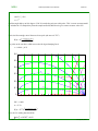
Problem: Place the following system in state-space form
a s 3 +a s 2 +a s+a
Y = ⎛⎝ s 4 +b3 s 3 +b2 s 2 +b1 s+b0 ⎞⎠ U
3
2
1
0
Controller Canonical Form:
Change the problem to
X = ⎛⎝ s 4 +b s 3 +b1s 2 +b s+b ⎞⎠ U
3
2
1
0
Y = (a 3 s 3 + a 2 s 2 + a 1 s + a 0 )X
Solve for the highest derivative of X:
s 4 X = U − b 3 s 3 X + b 2 s 2 X + b 1 sX + b 0 X
Integrate s4X four tiems to get X: (note: x' means
x''''
1
s
x'''
1
s
x''
x'
1
s
dx
)
dt
x
1
s
Create s4X from U and its derivatives
x''''
1
s
x'''
1
s
x''
1
s
x'
1
s
x
-b3
-b2
-b1
-b0
Create Y from the derivatives of X:
JSG
5
rev August 17, 2009
NDSU
State Space & Canonical Forms
ECE 461
c3
c2
Y
c1
U
x''''
1
s
x'''
1
s
X4
x''
1
s
X3
x'
1
s
X2
x
X1
c0
-b3
-b2
-b1
-b0
Controller Canonical Form
State Space Form: Define a state to be the output of each integrator (shown in red above). This gives
sX 1 = X 2
sX 2 = X 3
sX 3 = X 4
sX 4 = U − b 3 X 4 + b 2 X 3 + b 1 X 2 + b 0 X 1
or in matrix form:
⎡
⎢
s ⎢⎢
⎢
⎢
⎣
X1
X2
X3
X4
⎤ ⎡ 0
1
0
0 ⎤⎡
⎥ ⎢ 0
0
1
0 ⎥⎥ ⎢⎢
⎥=⎢
⎥ ⎢
⎥⎢
⎥ ⎢ 0
0
0
1 ⎥⎢
⎥ ⎢
⎥⎢
⎦ ⎣ −b 0 −b 1 −b 2 −b 3 ⎦ ⎣
⎡
⎢
Y = ⎡⎣ c 0 c 1 c 2 c 3 ⎤⎦ ⎢⎢
⎢
⎢
⎣
X1
X2
X3
X4
X1
X2
X3
X4
⎤ ⎡
⎥ ⎢
⎥+⎢
⎥ ⎢
⎥ ⎢
⎥ ⎢
⎦ ⎣
0
0
0
1
⎤
⎥
⎥U
⎥
⎥
⎥
⎦
⎤
⎥
⎥ + [0]U
⎥
⎥
⎥
⎦
Note that you can write this state-space model by inspection from the transfer function:
a s 3 +a s 2 +a s+a
Y = ⎛⎝ s 4 +b3 s 3 +b2 s 2 +b1 s+b0 ⎞⎠ U
3
2
1
0
This is what MATLAB uses to store transfer functions since it's so easy to determine once you know the transfer
function. It's also easy to convert from controller canonical form to the transfer function.
This form is called 'controller form' since the input, U, can set the states at will. For example, if
u(t) = δ(t)
the output of the first integrator jumps to 1 at t=0+. If
JSG
6
rev August 17, 2009
NDSU
State Space & Canonical Forms
ECE 461
u(t) = dtd (δ(t))
(termed a doublet), the output of the second integrator jumps to 1 at t=0+.
This form also has some of the worst numerical properties. Nothing is free.
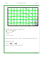
Observer Canonical Form:
If you transpose controller canonical form you get observer form:
A o = (A c ) T
B o = (C c ) T
C o = (B c ) T
or
⎡
⎢
s ⎢⎢
⎢
⎢
⎣
X1
X2
X3
X4
⎤ ⎡0
⎥ ⎢1
⎥=⎢
⎥ ⎢
⎥ ⎢0
⎥ ⎢
⎦ ⎣0
0
0
1
0
−b 0
−b 1
−b 2
−b 3
0
0
0
1
⎡
⎢
Y = ⎡⎣ 0 0 0 1 ⎤⎦ ⎢⎢
⎢
⎢
⎣
X1
X2
X3
X4
⎤⎡
⎥⎢
⎥⎢
⎥⎢
⎥⎢
⎥⎢
⎦⎣
X1
X2
X3
X4
⎤ ⎡
⎥ ⎢
⎥+⎢
⎥ ⎢
⎥ ⎢
⎥ ⎢
⎦ ⎣
c0
c1
c2
c3
⎤
⎥
⎥U
⎥
⎥
⎥
⎦
⎤
⎥
⎥ + [0]U
⎥
⎥
⎥
⎦
The block-diagram version looks like the following:
sX 1 = −b 0 X 4 + c 0 U
etc.
U
c0
1
X1
X2
1
s
-b0
c2
c1
c3
1
s
X3
1
s
-b1
-b2
X4
Y
s
-b3
Observer Canonical Form
JSG
7
rev August 17, 2009
NDSU
State Space & Canonical Forms
ECE 461
The nice thing about observer canonical form is you can determine all four states by measuring the output, Y, and
its derivatives.
Cascade Form:
Assume the transfer function factors as
c0
⎞U
Y = ⎛⎝ (s+p 1 )(s+p 2 )(s+p
3 )(s+p 4 ) ⎠
Treat this as four sytems cascaded:
c
X 1 = ⎛⎝ s+p0 1 ⎞⎠ U
X 2 = ⎛⎝ s+p1 2 ⎞⎠ X 1
X 3 = ⎛⎝ s+p1 3 ⎞⎠ X 2
X 4 = ⎛⎝ s+p1 4 ⎞⎠ X 3
The block diagram model looks like the following:
U
1
c0
X1
X2
1
s
s
-p1
-p2
1
X3
1
s
s
-p3
-p4
X4 Y
The state-space model is:
⎡
⎢
s ⎢⎢
⎢
⎢
⎣
X1
X2
X3
X4
⎤ ⎡ −p 1 1
0
0
⎥ ⎢ 0 −p 1
0
2
⎥=⎢
⎥ ⎢
⎥ ⎢ 0
0 −p 3 1
⎥ ⎢
0
0 −p 4
⎦ ⎣ 0
⎡
⎢
Y = ⎡⎣ 0 0 0 1 ⎤⎦ ⎢⎢
⎢
⎢
⎣
X1
X2
X3
X4
⎤⎡
⎥⎢
⎥⎢
⎥⎢
⎥⎢
⎥⎢
⎦⎣
X1
X2
X3
X4
⎤ ⎡
⎥ ⎢
⎥+⎢
⎥ ⎢
⎥ ⎢
⎥ ⎢
⎦ ⎣
c0
0
0
0
⎤
⎥
⎥U
⎥
⎥
⎥
⎦
⎤
⎥
⎥ + [0]U
⎥
⎥
⎥
⎦
The nice thing about cascade form is it has very good numerical properties. You can also determine the poles of
the system by inspection: they're the values on the diagonal.
JSG
8
rev August 17, 2009
NDSU
State Space & Canonical Forms
ECE 461
Jordan Form:
Assume the transfer function can be expressed using partial fractions as
a
a
a
a
Y = ⎛⎝ ⎛⎝ s+p1 1 ⎞⎠ + ⎛⎝ s+p2 2 ⎞⎠ + ⎛⎝ s+p3 3 ⎞⎠ + ⎛⎝ s+p4 4 ⎞⎠ ⎞⎠ U
Treat this as four separate systems:
c
X 1 = ⎛⎝ s+p1 1 ⎞⎠ U
c
X 2 = ⎛⎝ s+p2 2 ⎞⎠ U
c
X 3 = ⎛⎝ s+p3 3 ⎞⎠ U
c
X 4 = ⎛⎝ s+p4 4 ⎞⎠ U
Y is then the sum of these four.
In block diagram form, Jordan form looks like the following:
1
c1
X1
s
-p1
1
c2
X2
s
U
Y
-p2
1
c3
X3
s
-p3
1
c4
X4
s
-p4
In state-space, this looks like:
JSG
9
rev August 17, 2009
NDSU
⎡
⎢
s ⎢⎢
⎢
⎢
⎣
X1
X2
X3
X4
State Space & Canonical Forms
⎤ ⎡ −p 1 0
0
0 ⎤⎡
⎥ ⎢ 0 −p 0
0 ⎥⎥ ⎢⎢
2
⎥=⎢
⎥ ⎢
⎥⎢
⎥ ⎢ 0
0 −p 3 0 ⎥ ⎢
⎥ ⎢
⎥⎢
0
0 −p 4 ⎦ ⎣
⎦ ⎣ 0
⎡
⎢
Y = ⎡⎣ 1 1 1 1 ⎤⎦ ⎢⎢
⎢
⎢
⎣
JSG
X1
X2
X3
X4
X1
X2
X3
X4
⎤ ⎡
⎥ ⎢
⎥+⎢
⎥ ⎢
⎥ ⎢
⎥ ⎢
⎦ ⎣
c1
c2
c3
c4
ECE 461
⎤
⎥
⎥U
⎥
⎥
⎥
⎦
⎤
⎥
⎥ + [0]U
⎥
⎥
⎥
⎦
10
rev August 17, 2009
NDSU
SciLab
ECE 461
SciLab
Objectives:
Be able to write your own function in SciLab
Input a system in packed form
Introduce the control system toolbox for SciLab
SciLab vs. Matlab:
SciLab and Matlab are pretty similar. Both have almost identical syntax. Both allow you to write your own
functions. SciLab is free, however, so you can install it on your home computer (and laptop, etc.) I like free.
To get your own copy of SciLab, search for SciLab from a web browser. I think the site is:
www.SciLab.org
Adding a function in SciLab:
Suppose you want to add a function 'dB' which is called as
y = dB(x)
In SciLab, go to File Change Current Directory. Change it to where your files are located.
Go to File Open a file. Open up a .sci file. Change it as follows:
JSG
1
September 8, 2009
NDSU
SciLab
ECE 461
note: SciLab is very picky.
The file name must patch the function name
Both are case sensitive
Once you have a file you're happy with, add this to SciLab (execute - load into Scilab)
You now have the function 'dB' which you can call in Scilab!
note: If you create a bunch of files, you can load them into Scilab one at a time. Save the environment. When
you restart Scilab, load the environment and all the functions that were in Scilab before are there again.
JSG
2
September 8, 2009
NDSU
SciLab
ECE 461
SciLab Control Systems Toolbox:
The control systems toolbox in Scilab is free for you to use. It's still a work in progress (started Sep 6, 2009), so
more stuff should appear shortly.
The idea is to let you add and manipulate transfer functions in Scilab. The functions are as follows:
note: You probably have to
Copy the control toolbox files over to your computer and unzip them
In SciLab, load each file into Scilab one at a time.
Save your environment.
Yea, loading in each file is a pain, but you only have to do it once. From then on, just load the environment.
poly: Find a polynomial which has a given set of poles:
->P = poly([-1,-2,-3,-4])
P =
1.
10.
35.
50.
24.
s + 10s + 35s + 50s + 24 = (s + 1)(s + 2)(s + 3)(s + 4)
4
3
2
sspack: Save a system in packed matrix form
-->G = sspack(A,B,C,D)
G =
0.
- 10.
1.
1.
- 2.
0.
0.
20.
0.
⎡A B ⎤
⎥ . This assumes a single-input, single-output system, so the last row and last column gives
⎣C D ⎦
note: G = ⎢
your B, C, and D.
ssunpack: Extract the A, B, C, D matrix from G:
-->[A,B,C,D] = ssunpack(G)
tf2ss2: Input a system in transfer funciton form. For example: G = ⎛⎝
5s+6 ⎞
s 2 +3s+2 ⎠
-->G = tf2ss2([5,6],[1,3,2])
G =
0.
- 2.
6.
JSG
1.
- 3.
5.
0.
1.
0.
3
September 8, 2009
NDSU
SciLab
ECE 461
5(s+2)
zp2ss: Input a system in zeros, poles, gain form: For example: G = ⎛⎝ (s+3)(s+4) ⎞⎠
-->G = zp2ss(-2,[-3,-4],5)
G =
0.
- 12.
10.
1.
- 7.
5.
0.
1.
0.
eig: Compute the poles (eigenvalues) of a system in packed form:
-->eig(G)
ans =
- 3.
- 4.
5(s+2)
evalfr: Compute G(s). Find G = ⎛⎝ (s+3)(s+4) ⎞⎠
s=j3
-->G = zp2ss(-2,[-3,-4],5);
-->evalfr(G, j*3)
0.7666667 - 0.3666667i
bode2: Compute G(jw) at a bunch of frequencies:
-->w = logspace(-2,2,100);
-->Gw = bode2(G,w);
-->plot(w,dB(Gw));
intcon: Connect two systems with unity feedback.
-->G
0.
JSG
1.
0.
4
September 8, 2009
NDSU
- 12.
10.
SciLab
- 7.
5.
ECE 461
1.
0.
-->intcon(G,3)
0.
- 42.
10.
1.
- 22.
5.
0.
3.
0.
rlocus: Plot the root locus for a unity feedback system with several gains:
k = logspace(-2,1,100);
locus = rlocus(G,k);
JSG
5
September 8, 2009
NDSU
SciLab
ECE 461
step: Compute the step response of a system
-->G = tf2ss2(100,[1,2,20])
-->t = [0:0.01:5]';
-->y = step(G,t);
-->plot(t,y);
Nichols: Plot the Nichols chart of G(jw) along with an M-circle Mm = 2 = 6dB.
G = zp2ss([],[0,-5,-20],1000);
w = logspace(-1,1,100);
Gw = bode2(G,w);
nichols(Gw,2);
leastsq(): Minimization of a Function:
note: MATLAB's version is call fminsearch().
A very useful tool in SciLab is the funciton leastsq(). This is a nonlinear optimization routine that finds the
minimum of a function. For example, suppose you wanted to find the solution to
JSG
6
September 8, 2009
NDSU
SciLab
ECE 461
x ln(x) + x = 3
First, create a function in SciLab which returns a minimum for x solving the above equation. One way to do this
is compute the error and square it:
y = (x ln(x) + x − 3) 2
In SciLab, create a function (I called it 'cost2.sci' for lack of a better name).
function y = cost2(x)
// y = cost(z)
e = x*log(x) + x - 3;
y = e*e;
endfunction
Execute and load this into SciLab. You can use trial and error to find x. Keep guessing until cost2 returns zero
-->cost2(2)
0.1492233
-->cost2(3)
10.862541
-->cost2(2.1)
0.4330541
-->cost2(1.9)
0.0142856
The answer is close to 1.9. Or, you can use leastsqfn
-->[e,x] = leastsq(cost2,1.7)
x =
1.8545507
e =
1.458D-31
The answer is 1.8545507.
Problem: Find the values of a..e which make the following transfer function as close to an ideal low pass filter
with a corner at 3 rad/sec
2
⎞
G(s) = ⎛⎝ s 3as+ds+bs+c
2 +es+c ⎠
Solution: Use leastsq(). Pass a 5x1 array containing a..e. Compute the difference in gain of G(s) from an ideal
low pass filter. Return the sum squared difference.
function y = cost(z)
// y = cost(z)
// call with [e,y] = leastsq(cost,[1,2,1,4,4])
a
b
c
d
e
j
w
s
JSG
=
=
=
=
=
=
=
=
z(1);
z(2);
z(3);
z(4);
z(5);
sqrt(-1);
[0:0.1:10]';
j*w;
7
September 8, 2009
NDSU
SciLab
ECE 461
Gideal = 1*(w<3);
Gs = (a*s.^2 + b*s + c) ./ (s.^3 + d*s.^2 + e*s + c);
plot(w,Gideal,w,abs(Gs));
e = abs(Gideal) - abs(Gs);
y = sum(e.^2);
endfunction
Note that the plot command plots the ideal low pass filter along with your current guess. This slows down the
routine, but it's interesting to see how the optimization routine progresses.
The result is
->[e,y] = leastsq(cost,[1,2,1,4,4])
y =
0.5571236
8.901D-08 9.9814208
e =
1.2097191
2.3253089
7.8440956
so
0.557s 2 +9.98
⎞
G(s) = ⎛⎝ s 3 +2.325s
2 +7844s+9.98 ⎠
with the following gain vs. frequency:
JSG
8
September 8, 2009
NDSU
Modeling Electircal Circuits
ECE 461
Modeling Electrical Circuits
Objective:
Be able to write the voltage node equations for an electrical circuit
Be able to place these dynamics in state-space form
Be able to find the transfer funciton for an electrical circuit
Electronic Circuits:
Circuits with elements which store energy (inductors and capacitors) are dynamic systems (as opposed to static
systems which have only resistors). The transfer function for a circuit can be obtained by substituting the LaPlace
value of the element's impedance:
V/I Relationship
LaPlace value of
Resistance
V=IR
R
Resistor
∫ I ⋅ dt
Capacitor
V=
Inductor
V = L dI
dt
1
C
1 / sC
Ls
Current loops, voltage nodes, or other circuit analysis techniques can then be used to find the transfer function.
Example:
Find the transfer function from Vi to Vo:
R1
R2
a
b
+
Vi
+
1/Cs
Ls
-
Vo
-
Solution:
Writing the voltage node equations at nodes a and b:
a)
⎛ V a −V i ⎞ + ⎛ V a ⎞ + ⎛ V a −V b ⎞ = 0
⎝ R 1 ⎠ ⎝ Ls ⎠ ⎝ R 2 ⎠
b)
⎛ V b −V a ⎞ + ⎛ V b ⎞ = 0
⎝ R 2 ⎠ ⎝ 1/Cs ⎠
JSG
1
rev September 17, 2007
NDSU
Modeling Electircal Circuits
ECE 461
Separating into common terms results in
a)
⎛ 1 + 1 + 1 ⎞ Va − ⎛ 1 ⎞ Vi − ⎛ 1 ⎞ Vb = 0
⎝ R 1 Ls R 2 ⎠
⎝ R1 ⎠
⎝ R2 ⎠
b)
⎛ 1 + Cs ⎞ V b − ⎛ 1 ⎞ V a = 0
⎝ R2
⎠
⎝ R2 ⎠
Note that a pattern emerges (which will follow in mechanical examples:
At Node a:
(The sum of the admittance's to node a)Va - (the sum of the admittances from node a to b)Vb - ...)
= (The current to node a)
Now, you can solve 2 equations for 2 unknowns by getting Va to drop out. For example,
AV a − BV i − CV b = 0
(x C)
+
DV b − CV a = 0
=
−(BC)V i + (AC − C 2 )V b = 0
(xA)
BC ⎞
V b = ⎛⎝ AC−C
2 ⎠ Vi
⎛ 1 ⎞⎛ 1 ⎞
⎛
⎞
⎝ R1 ⎠ ⎝ R2 ⎠
⎟ V = G(s) ⋅ V i
V b = ⎜⎜
⎜ ⎛ 1 + 1 + 1 ⎞ ⎛ 1 ⎞ − ⎛ 1 ⎞ 2 ⎟⎟ i
⎝ ⎝ R1 R2 Ls ⎠ ⎝ R2 ⎠ ⎝ R2 ⎠ ⎠
If you live long enough, you can simplify G(s).
Placing the Dynamics in State Space Form
If MATLAB is available, you can find the transfer funciton using state-space representation. The goal is to place
the system in the form of
sX = AX + BU
Y = CX + DU
For example, take the circuit above. Rewrite the two dynamics equations as
⎛ Ls + 1 + Ls ⎞ V a − ⎛ Ls ⎞ V i − ⎛ Ls ⎞ V b = 0
R2 ⎠
⎝ R1
⎝ R1 ⎠
⎝ R2 ⎠
JSG
2
rev September 17, 2007
NDSU
Modeling Electircal Circuits
ECE 461
⎛ L + L ⎞ sV a − ⎛ L ⎞ sV i − ⎛ L ⎞ sV b = −V a
⎝ R1 R2 ⎠
⎝ R1 ⎠
⎝ R2 ⎠
(a)
(C)sV b = ⎛⎝ R−1 ⎞⎠ V b + ⎛⎝ R1 ⎞⎠ V a = 0
2
2
(b)
In matrix form
⎡ ⎛ L + L ⎞ ⎛ −L ⎞
⎢ ⎝ R1 R2 ⎠ ⎝ R1 ⎠
⎢
⎢
0
C
⎣
L
⎤⎡
⎥ sV a ⎤ = ⎡⎢ −1 0 ⎤⎥ ⎡ V a ⎤ + ⎡⎢ R 2 ⎤⎥ sV
⎥⎢
⎥ ⎢ 1 −1 ⎥ ⎢
⎥ ⎢
⎥ i
⎥ ⎣ sV b ⎦ ⎢⎣ R 2 R 2 ⎥⎦ ⎣ V b ⎦ ⎢⎣ 0 ⎥⎦
⎦
Inverting the matrix on the left:
⎞
⎡ sV a ⎤ ⎡⎢ ⎛⎝ RL + RL ⎞⎠ ⎛⎝ −L
R1 ⎠
1
2
=
⎢
⎥ ⎢
⎣ sV b ⎦ ⎢⎣
0
C
⎤
⎥
⎥
⎥
⎦
−1
⎡⎢ −1 0 ⎤⎥ ⎡ V a ⎤ ⎡⎢ ⎛ L + L ⎞ ⎛ −L ⎞
⎢⎢ 1 −1 ⎥⎥ ⎢
⎥ + ⎢ ⎝ R1 R2 ⎠ ⎝ R1 ⎠
V
⎣ R 2 R 2 ⎦ ⎣ b ⎦ ⎢⎣
0
C
⎤
⎥
⎥
⎥
⎦
−1
⎡⎢ RL ⎤
⎢⎢ 2 ⎥⎥⎥ sV i
⎣ 0 ⎦
⎡V ⎤
Y = ⎡⎣ 0 1 ⎤⎦ ⎢ a ⎥ + [0]sV i
⎣ Vb ⎦
(trick): The input is the derivative of Vi. If you ignore this 's' term times Vi, you're off by a derivative. Let's be
off by a derivative for now.
sX = AX + BU
Y ∗ = CX
If you differentiate the output, you get the derivative back
sY ∗ = CsX = C(AX + BU)
so change the output to add this derivative:
Y = (CA)X + (CB)U
The state space dynamics are then
⎡ ⎛ L + L ⎞ ⎛ −L ⎞
A = ⎢⎢ ⎝ R 1 R 2 ⎠ ⎝ R 1 ⎠
⎢
0
C
⎣
⎤
⎥
⎥
⎥
⎦
−1
⎡ ⎛ L + L ⎞ ⎛ −L ⎞
B = ⎢⎢ ⎝ R 1 R 2 ⎠ ⎝ R 1 ⎠
⎢
0
C
⎣
⎤
⎥
⎥
⎥
⎦
−1
⎡⎢ −1 0 ⎤⎥
⎢⎢ 1 −1 ⎥⎥
⎣ R2 R2 ⎦
⎡⎢ RL ⎤
⎢⎢ 2 ⎥⎥⎥
⎣ 0 ⎦
C = ⎡⎣ 0 1 ⎤⎦ A
D = ⎡⎣ 0 1 ⎤⎦ B
JSG
3
rev September 17, 2007
NDSU
Modeling: Heat Equation
ECE 461
Systems Modeled by the Heat Equation
Objectives:
Be able to
Write the differential equations for a system modeled by the heat equation
Write the electrical RC circuit equivalent for such a system
Write the state-space equations for a heat system
Find the transfer function using MATLAB
Given the transfer function, predict how the system will respond to a step input
Definition: The Heat Equation:
If you want to model the temperature behaviour of a system, you could break the system into a large number of
finite elements. The temperature at each element is proportional to the energy in that element. The energy at this
node can flow to neighboring elements and is described by a first-order differential equation.
At each node:
dx i
dt
= −a ii x i + Σ a ij x j
i≠j
where xi is the temperature at node i and aij are real positive constants:
a ij > 0
a ii > Σ a ij
i≠j
The last requirement is conservation of energy: the energy gained by neighboring nodes cannot be greater than
the energy lost at node i. If could be less (if you have a lossy, i.e. poorly insulated) system, however.
RC Circuit Analogy:
The electrical circuit which also satisfied the heat equation is a passive RC network with capacitors to ground and
resistors connecting the capacitors. For example, suppose you wanted to model the temperature along a long rod.
If you treat this as five finite elements, each element has
Thermal intertia: the energy stored is proportional to the temperature at that node, and
Thermal conductivity: Between elements, energy can flow and is proportional to the temperature
difference between adjacent nodes times the thermal conductivity.
The electrical analogy is an RC network where each voltage node has
A capacitor to ground: the energy stored is porportional to the voltage at the node, and
Resistance: between each capacitor, resistors are palced. The current flow is proportional to the voltage
between adjacent nodes times the electrical conductuvity of that resistor.
The analogy is
Heat
JSG
Thermal Inertia
(J / degree)
Temperature
(degrees C)
1
Heat Flow
(Watts)
Thermal Resistance
(degree C / Watt)
rev September 1, 2007
NDSU
Modeling: Heat Equation
Electrical
Capacitance
(J / volt)
Voltage
(Volts)
ECE 461
Current
(Amps)
Resistance (R)
(Ohm = Volts / Amp)
1-Dimenstional Example:
For example, find the mathematical model for the temperature along a long thin rod. For convenience, assume
you split this rod into five finite elements. For each element,
Assume each element has a thermal inertia of C Joules / degree. (the volume of each element times the
thermal capacitance of the material)
Between elements, assume that 1 Watts flows if the temperature difference is R degrees. (Thermal
conductivity times area divided by distance).
u
x1
x2
x3
x4
x5
The elecrical analogy is an RC circuit is as follows:
u
x1
R01
u
+
-
x2
x1
C1
R12
x3
R23
x2
x4
x3
C2
R34
C3
x4
x5
R45
C4
x5
C5
The differential equations for this system are then:
C1
dx 1
dt
= − ⎛⎝ R101 + R112 ⎞⎠ x 1 + ⎛⎝ R112 ⎞⎠ x 2 + ⎛⎝ R101 ⎞⎠ u
C2
dx 2
dt
= − ⎛⎝ R112 + R123 ⎞⎠ x 2 + ⎛⎝ R112 ⎞⎠ x 1 + ⎛⎝ R123 ⎞⎠ x 3
C3
dx 3
dt
= − ⎛⎝ R123 + R134 ⎞⎠ x 3 + ⎛⎝ R123 ⎞⎠ x 2 + ⎛⎝ R134 ⎞⎠ x 4
C4
dx 4
dt
= − ⎛⎝ R134 + R145 ⎞⎠ x 4 + ⎛⎝ R134 ⎞⎠ x 3 + ⎛⎝ R145 ⎞⎠ x 5
C5
dx 2
dt
= − ⎛⎝ R145 ⎞⎠ x 5 + ⎛⎝ R145 ⎞⎠ x 4
In State Space form:
JSG
2
rev September 1, 2007
NDSU
Modeling: Heat Equation
⎡ − ⎛ 1/R 01 +1/R 12 ⎞
⎛ 1/R 12 ⎞
0
0
0
C1
⎠
⎝ C1 ⎠
⎢ ⎝
⎢
⎡ x1 ⎤
1/R +1/R
⎛ 1/R 12 ⎞
⎛ 1/R 23 ⎞
− ⎛⎝ 12C 2 23 ⎞⎠
0
0
⎥ ⎢
⎢
⎝ C2 ⎠
⎝ C2 ⎠
x
⎢⎢ 2 ⎥⎥ ⎢⎢
1/R +1/R
⎛ 1/R 23 ⎞
⎛ 1/R 34 ⎞
0
s⎢ x3 ⎥ = ⎢
− ⎛⎝ 23C 3 34 ⎞⎠
0
⎝ C3 ⎠
⎝ C3 ⎠
⎥ ⎢
⎢
⎢ x4 ⎥ ⎢
1/R +1/R
1/R
⎛ 1/R 34 ⎞
⎥ ⎢
⎢
0
0
− ⎛⎝ 34C 4 45 ⎞⎠ ⎛⎝ C 445 ⎞⎠
C4 ⎠
⎝
x
5
⎦ ⎢
⎣
1/R
⎛ 1/R 45 ⎞
⎢
0
0
0
− ⎛⎝ C 545 ⎞⎠
⎝ C5 ⎠
⎣
ECE 461
⎤
⎥
⎥⎡
⎥⎢
⎥⎢
⎥⎢
⎥⎢
⎥ ⎢⎢
⎥
⎥⎢
⎥⎣
⎥
⎦
x1
x2
x3
x4
x5
⎤ ⎡ ⎛⎝ C 1R ⎞⎠
1 01
⎥ ⎢
⎥⎥ ⎢⎢
0
⎥+⎢
0
⎥ ⎢
⎥ ⎢
0
⎥ ⎢
⎦ ⎣
0
⎤
⎥
⎥
⎥
⎥u
⎥
⎥
⎥
⎦
If C = 0.01F and R = 10 Ohms,
⎡
⎢
⎢
s⎢
⎢
⎢
⎣
x1
x2
x3
x4
x5
⎤ ⎡ −20 10 0
0
0 ⎤⎡
⎥ ⎢ 10 −20 10 0
0 ⎥⎥ ⎢⎢
⎥ ⎢⎢
⎥ = ⎢⎢ 0 10 −20 10 0 ⎥⎥⎥ ⎢⎢⎢
⎥ ⎢ 0
0 10 −20 10 ⎥ ⎢
⎥ ⎢
⎥⎢
0
0 10 −10 ⎦ ⎣
⎦ ⎣ 0
x1
x2
x3
x4
x5
⎤ ⎡
⎥ ⎢
⎥⎥ ⎢⎢
⎥⎥ + ⎢⎢
⎥ ⎢
⎥ ⎢
⎦ ⎣
10
0
0
0
0
⎤
⎥
⎥⎥
⎥⎥ u
⎥
⎥
⎦
Note that this is a lossless system: there is no thermal conductivity bewteen the rod and the environment. This
shows up in the above matrix with each row adding to zero. If there were losses, the diagonal elements would be
more negative and the rows would sum to a negative number (lossy).
Problem: Estimate how this system will behave:
Solution: I need to know the systems dominant pole(s) and DC gain. In MATLAB:
A
B
C
D
=
=
=
=
[-20,10,0,0,0;10,-20,10,0,0;0,10,-20,10,0;0,0,10,-20,10;0,0,0,10,-10];
[10;0;0;0;0];
[0,0,0,0,1];
0;
eig(A)
{-0.8101, -6.9028, -17.1537, -28.3083, -36,8251}
DC = C*inv(A)*B
DC = 1.00000
The system has a DC gain of one. If the input is increased to 100C, the output will go to 100C as well.
The system has a dominant pole at -0.8101. It will take approximately 4.93 seconds (4/0.8101) to reach steady
state.
The dominant pole is real. There should be no overshoot or oscillations in the step response.
Problem: Determine the actual step response:
Solution: Using MATLAB:
G = ss(A,B,C,D);
zpk(G)
t = [0:0.1:10]';
y = step(G,t);
plot(t,y)
JSG
3
rev September 1, 2007
NDSU
Modeling: Heat Equation
ECE 461
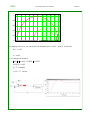
2-Dimenstional Heat Equations:
The above also works for plates (2 dimenstions), and solids (3-dimenstions). For example, find the heat flow for
a plate, modeled as five finite elements:
x1
x2
x3
x4
x5
x6
u
x2
X1
U
x3
+
-
x4
x5
x6
Assuming all resitances are 10 Ohms and C = 0.01F again,
⎡
⎢
⎢
⎢
s⎢
⎢
⎢
⎢
⎣
x1
x2
x3
x4
x5
x6
⎤ ⎡ −30
⎥ ⎢ 10
⎥ ⎢
⎥ ⎢ 0
⎥=⎢
⎥ ⎢ 10
⎥ ⎢ 0
⎥ ⎢
⎦ ⎣ 0
10 0 10 0
0 ⎤⎡
−30 10 0 10 0 ⎥⎥ ⎢⎢
10 −20 0
0 10 ⎥ ⎢
⎥⎢
0
0 −30 10 0 ⎥ ⎢
10 0 10 −30 10 ⎥ ⎢
⎥⎢
0 10 0 10 −20 ⎦ ⎣
x1
x2
x3
x4
x5
x6
⎤ ⎡
⎥ ⎢
⎥ ⎢
⎥ ⎢
⎥+⎢
⎥ ⎢
⎥ ⎢
⎥ ⎢
⎦ ⎣
10
0
0
10
0
0
⎤
⎥
⎥
⎥
⎥
⎥
⎥
⎥
⎦
Problem: Estimate what the step response from U to x3 will look like
Solution: In MATLAB:
A = [-30,10,0,10,0,0;10,-30,10,0,10,0;0,10,-20,0,0,10];
A = [A; A(:,[4,5,6,1,2,3]));
B = [10;0;0;10;0;0];
C = [0,0,1,0,0,0];
D = 0;
eig(A)
-32.46, -35.54, -21.98, -15.54, -52.46, -1.98
DC = -C*inv(A)*B
DC = 1.0000
The system has a DC gain of one. If the input is increased to 100C, the output will go to 100C as well.
JSG
4
rev September 1, 2007
NDSU
Modeling: Heat Equation
ECE 461
The system has a dominant pole at -1.98. It will take approximately 2.02 seconds (4/1.98) to reach steady
state.
The dominant pole is real. There should be no overshoot or oscillations in the step response.
JSG
5
rev September 1, 2007
NDSU
Mechanical Systems Systems
ECE 461
Translational Mechanical Systems:
Mass and spring systems also are dynamic systems. One way to model these systems is to
1) Replace the mass, spring, and friction terms with their LaPlace admittance,
2) Redraw the system as an electric circuit, and
3) Write the voltage node equations.
The LaPlace admittance's come from modeling the system as
Force = mass * acceleration
F=ZX
(F = force, Z = admittance, X = displacement)
which has the electrical analog
I=GV
(current = admittance * voltage).
Mechanical System
Electrical Analog
Force in the positive
direction
Current to the node
Displacement in the
positive direction
Positive voltage
Mass, (see below)
Admittance
F=ZX
Relationship
LaPlace value of
Addmittance
Mass
f = m x''
s2 m
Spring
f=kx
k
Friction
f = B x'
f = fv x'
sB
s fv
Example:
Write the equations of motion for the following mass and spring system:
K1
B3
m1
K3
K2
m2
f
B1
JSG
x1
B2
1
x2
rev July 16, 2009
NDSU
Mechanical Systems Systems
ECE 461
Solution:
Step 1: Draw the circuit equivalent:
K2
X1
X2
s B1
F
M1 s²
K1
B2 s
B3 s
K3
M2 s²
Step 2: Write the voltage node equations. From before
(The sum of the admittance's to node a)Va - (the sum of the admittances from node a to b)Vb - ...)
= (The current to node a)multiply a: times (1/R2) and
(K 1 + B 1 s + M 1 s 2 + K 2 + B 3 s)X 1 − (K 2 + B 3 s)X 2 = F
(M 2 s 2 + B 2 s + K 3 + K 2 + B 3 s)X 2 − (K 2 + B 3 s)X 1 = 0
Step 3: Solve to find the output as a function of the input. If X2 is the output and F is the input, solve to find
X 1 = G(s) ⋅ F
For this system use dummy variables for the coefficients of X1 and X2 in the above equations:
AX 1 − BX 2 = F
(multiply by B)
−BX 1 + CX 2 = 0
(multiply by A and add)
(−B 2 + AC)X 2 = BF
=
B ⎞
X 2 = ⎛⎝ AC−B
2⎠F
or substituting in the values of A, B, C
⎛
⎞
K 2 +B 3 s
X2 = ⎜ ⎛
⎟F
⎝ ⎝ K 1 +B 1 s+M 1 s 2 +K 2 +B 3 s ⎞⎠ ⎛⎝ M 2 s 2 +B 2 s+K 3 +K 2 +B 3 s ⎞⎠ −(K 2 +B 3 s) 2 ⎠
JSG
2
rev July 16, 2009
NDSU
Mechanical Systems Systems
ECE 461
Rotational Systems
Dynamics of Rotational Systems
Rotational systems are very similar to translational systems. The analogy used is to treat inertia, springs, and
friction as admittanced. The only difference is the standard symbol for intertia (J vs M), spring (K vs k) and
friction (D vs B).
F=ZX
Relationship
LaPlace value of
Addmittance
Mass
f = J x''
Js2
Spring
f=Kx
K
Friction
f = D x'
f = fv x'
Ds
s fv
Rotational systems often times have gears as well. A gear will speed up or slow down the rotation of a system by
a factor N. Two nodes conected with a single gear only have one degree of freedom: once the angle of one node
is defined, the angle of the other is fexed by the gear. The relationship between the angle of two nodes connected
with a gear is
N1θ1 = N2θ2
which is signified as:
Circuit Model
T1 Q1
N1
Q1
N1:N2
Q2
Q2
T2
N2
For example, if N2 is larger then N1, Q2 will be slower than Q1 by the turn ratio
N1Q1 = N2Q2
N
Q 2 = ⎛⎝ N 12 ⎞⎠ Q 1
Torqe increases if you go from a small (fast spinning) gear to a larger one as the turn ratio
N
T 2 = ⎛⎝ N 21 ⎞⎠ T 1
If there is an admittance at Q1
T1 = Y1Q1
this will be seen at node 2 as
⎛ N1 ⎞ T 2 = Y 1 ⎛ ⎛ N2 ⎞ Q 2 ⎞
⎝ N2 ⎠
⎝ ⎝ N1 ⎠ ⎠
JSG
3
rev July 16, 2009
NDSU
Mechanical Systems Systems
ECE 461
2
N
T 2 = ⎛⎝ N 21 ⎞⎠ Q 2
The admittance seen through a gear is changed by the turn ratio squared.
The impedance seen on the rapidly spinning side is reduced by the turn ratio squared.
Example: Determine the transfer function from T1 to Q1:
T1 Q1 J1
N1
Q2
T2
K2
J3
J2
N2
D1
Q3
First draw the circuit diagram using LaPlace admittances.
K2
Q1
Q2
Q3
J2s2
J3s^2
1:5
T1
J1s2
D1s
Next, transfer all the admittances through the gear to Q1's side. Since you're going right to left, the admittances
will transfer as ⎛⎝ 15 ⎞⎠
2
0.04K2
Q1
T1
5Q2
J1s
5Q3
0.04J3s2
0.04J2s2
0.04D1s
You can now write your voltage node equations
JSG
4
rev July 16, 2009
NDSU
Mechanical Systems Systems
ECE 461
(J 1 s 2 + 0.04J 2 s 2 + 0.04K 2 )Q 1 − (0.04K 2 )Q ∗3 = T 1
(0.04J 3 s 2 + 0.04D 1 s + 0.04K 2 )Q ∗3 − (0.04K 2 )Q 1 = 0
Since the admittance translates as the gear ratio squared, it allows you to minimize the effect of whatever is on the
other side of the gear by using a large gear reduction. This is often done in robotics, where 300:1 gear reduction
is not uncommon (the motor sees the outside world, scaled down by a factor of 90,000!)
JSG
5
rev July 16, 2009
NDSU
Mechanical Systems Systems
ECE 461
Servo Motors
Transfer Functions for DC Servo Motors:
The equations that describe a DC servo motor are
Back EMF = K t ω = K t
dQ
dt
Torque = K t I a
where Kt is the torque constant, Q is the angle, and Ia is the armature current. The circuit model for a DC servo
motor is then
Ra
Las
Q
Ia
KtIa
Va
+
Kt*dQ/dt
Js 2
Ds
-
or
V a = K t (sQ) + (R a + L a s)I a
K t I a = (Js 2 + Ds)Q
Solving gives
Kt
⎞V
Q = ⎛⎝ 1s ⎞⎠ ⎛⎝
a
(Js+D)(L a s+R a )+K 2t ⎠
if the output is angle (Q) or
ω=
dQ
dt
Kt
⎞V
= ⎛⎝
a
(Js+D)(L a s+R a )+K 2t ⎠
if the output is speed.
Example: Determine the transfer function for a DC servo motor with the following specifications:
(http://www.servosystems.com/electrocraft_dcbrush_rdm103.htm)
K t = 0.03Nm/A
Terminal resistance = 1.6 (Ra)
Armature inductance = 4.1mH (La)
Rotor Inertia = 0.008 oz-in/sec/sec
Damping Contant = 0.25 oz-in/krpm
Torque Constant = 13.7 oz-in/amp
Peak current = 34 amps
Max operating speed = 6000 rpm
JSG
ugh - english units
double ugh
6
rev July 16, 2009
NDSU
Mechanical Systems Systems
ECE 461
You need to translate to metric:
Kt:
⎛ 1m ⎞ ⎛ 1lb ⎞ ⎛ 0.454kg ⎞ ⎛ 9.8N ⎞
⎛ N⋅m ⎞
13.7 oz−in
amp ⎝ 39.4in ⎠ ⎝ 16oz ⎠ ⎝ lb ⎠ ⎝ kg ⎠ = 0.0967 ⎝ A ⎠
D:
⎞ ⎛ 1Nm ⎞ ⎛ 60 sec ⎞ ⎛ krev ⎞ ⎛ rev ⎞ = 1.68 ⋅ 10 −5 ⎛ Nm ⎞
0.25 ⎛⎝ oz⋅in⋅min
krev ⎠ ⎝ 141.7oz−in ⎠ ⎝ min ⎠ ⎝ 1000rev ⎠ ⎝ 2πrad ⎠
⎝ rad/ sec ⎠
J:
⎞ ⎛ Nm ⎞ ⎛ kg ⎞ = 5.76 ⋅ 10 −6 ⎛ kg⋅m ⎞
0.008 ⎛⎝ oz−in
⎝ s2 ⎠
sec 2 ⎠ ⎝ 141.7oz−in ⎠ ⎝ 9.8N ⎠
Plugging in numbers:
2
10.31(630) 2
⎞V = ⎛
⎞V
Q = ⎛⎝ s(s 210.31⋅630
2
⎠
⎝
⎠
s(s+196.5+j598)(s+196.5−j598)
+393s+630 )
This means....
If you apply a constant +12V to the motor, the motor spins at a speed of 123.72 rad/sec. (10.31*12)
It takes about 20ms for the motor to get up to speed (Ts = 4/196)
The motor will overshoot it's final speed (123 rad/sec) by 35% (damping ratio = 0.3119)
JSG
7
rev July 16, 2009
NDSU
LaGrange Formulation of Dynamics
ECE 461
LaGrangian Formulation of System Dynamics
Find the dynamics of a nonlinear system:
Circuit analysis tools work for simple lumped systems. For more complex systems, especially nonlinear ones,
this approach fails. The Lagrangian formulation for system dynamics is a way to deal with any system.
Definitions:
KE
Kinetic Energy in the system
PE
Potential Energy
∂
∂t
The partial derivative with respect to 't'. All other variables are treated as constants.
d
dt
The full derivative with respect to t.
d
dt
L
=
∂ ∂x
∂x ∂t
∂y
+ ∂y∂ ∂t + ∂z∂ ∂z
∂t + ...
Lagrangian = KE - PE
Procedure:
1) Define the kinetic and potential energy in the system.
2) Form the Lagrangian:
L = KE − PE
3) The input is then
∂L ⎞
∂L
−
F i = dtd ⎛⎝ ∂x
.
∂x
i
i⎠
where Fi is the input to state xi. Note that
If xi is a position, Fi is a force.
If xi is an angle, Fi is a torque
JSG
1
rev 02/27/02
NDSU
LaGrange Formulation of Dynamics
ECE 461
Example:
Find the dynamics for the following system: A 1kg mass swings from a gantry which weighs 2kg. The length of
the rope is 1m.
x
2kg
F
1m
q
y2
1kg
x2
1) Write the energy in the system
Mass #1:
x1 = x
y1 = 0
.
KE 1 = 12 mv 2 = 12 ⋅ 2 ⋅ x 2
PE 1 = mgh = 0
Mass #2
x 2 = x 1 + sin θ
y 2 = 1 − cos θ
.
.
.
x 2 = x 1 + (cos θ)θ
.
.
y 2 = (sin θ)θ
.
.
KE 2 = 12 ⎛⎝ x 22 + y 22 ⎞⎠
.
.
.
. .
KE 2 = 12 ⎛⎝ x 21 + 2x 1 θ 1 cos θ + cos 2 θ ⋅ θ 2 + sin 2 θ ⋅ θ 2 ⎞⎠
.
.
. .
KE 2 = 12 ⎛⎝ x 21 + 2x 1 θ 1 cos θ + θ 2 ⎞⎠
PE 2 = mgh = gy 2
PE 2 = g − g cos θ
So, the Lagrangian is
JSG
2
rev 02/27/02
NDSU
LaGrange Formulation of Dynamics
ECE 461
.
.
.
..
L = ⎛⎝ x 2 + 12 ⎛⎝ x 2 + 2xθ cos θ + θ 2 ⎞⎠ ⎞⎠ − (g − g cos θ)
The force on the base is
F=
d ⎛ ∂L ⎞
.
dt ⎝ ∂x ⎠
F=
.
d⎛ .
2x + x
dt ⎝
− ∂L
∂x
.
+ 2θ cos θ ⎞⎠ − 0
.
F = 3ẍ + 2θ̈ cos θ − 2θ 2 sin θ
The torque on the rod is
T=
d ⎛ ∂L ⎞
.
dt ⎝ ∂θ ⎠
T=
d ⎛.
x cos θ +
dt ⎝
− ∂L
∂θ
.
..
θ ⎞⎠ − xθ sin θ − 9.8 sin θ
..
..
T = ẍ cos θ + xθ sin θ + θ̈ − xθ sin θ − g sin θ
So, the dynamics are
.
⎡ 3 2 cos θ ⎤ ⎡ ẍ ⎤ ⎡ 2θ 2 sin θ ⎤ ⎡ 1 ⎤
⎢
⎥⎢ ⎥ = ⎢
⎥ + ⎢ ⎥F
1
⎣ cos θ
⎦ ⎣ θ̈ ⎦ ⎣ g sin θ ⎦ ⎣ 0 ⎦
JSG
3
rev 02/27/02
NDSU
LaGrange Formulation of Dynamics
ECE 461
Linear Model
For small perturbations about 0,
sin θ ≈ θ
cos θ ≈ 1
.
θ2 ≈ 0
g = 9.8 m/s2
The dynamics linearized about zero are then
⎡ 3 2 ⎤ ⎡ ẍ ⎤ ⎡ 0 ⎤ ⎡ 1 ⎤
⎢
⎥⎢ ⎥ = ⎢
⎥ + ⎢ ⎥F
⎣ 1 1 ⎦ ⎣ θ̈ ⎦ ⎣ 9.8θ ⎦ ⎣ 0 ⎦
⎡ ẍ ⎤ ⎡ 1 −2 ⎤ ⎛ ⎡ 0 ⎤ ⎡ 1 ⎤ ⎞
⎢ ⎥=⎢
⎥⎜⎢
⎥ + ⎢ ⎥F⎟
⎣ θ̈ ⎦ ⎣ −1 3 ⎦ ⎝ ⎣ 9.8θ ⎦ ⎣ 0 ⎦ ⎠
or
⎡ ẍ ⎤ ⎡ −19.6θ + F ⎤
⎥
⎢ ⎥=⎢
⎣ θ̈ ⎦ ⎣ 29.4θ − F ⎦
which is a linear differential equation. You can put this in state-space form:
⎡
⎢
s ⎢⎢
⎢
⎢
⎣
x
θ
x
θ
⎤ ⎡0 0 1
⎥ ⎢0 0 0
⎥=⎢
⎥ ⎢
⎥ ⎢ 0 −19.6 0
⎥ ⎢
⎦ ⎣ 0 29.4 0
0
1
0
0
⎤⎡
⎥⎢
⎥⎢
⎥⎢
⎥⎢
⎥⎢
⎦⎣
x
θ
x
θ
⎤ ⎡
⎥ ⎢
⎥+⎢
⎥ ⎢
⎥ ⎢
⎥ ⎢
⎦ ⎣
0
0
1
−1
⎤
⎥
⎥F
⎥
⎥
⎥
⎦
Note that the eigenvalues of 'A' are
{0, 0, 5.42, −5.42}
corresponding to an unstable system. Here, gravity is pulling up, causing the pendulum to fall. (A sign error in
'g').
Let g = -9.8 m/s2:
JSG
4
rev 02/27/02
NDSU
⎡
⎢
s ⎢⎢
⎢
⎢
⎣
LaGrange Formulation of Dynamics
x
θ
x
θ
⎤ ⎡0 0 1
⎥ ⎢0 0 0
⎥=⎢
⎥ ⎢
⎥ ⎢ 0 19.6 0
⎥ ⎢
⎦ ⎣ 0 −29.4 0
0
1
0
0
⎤⎡
⎥⎢
⎥⎢
⎥⎢
⎥⎢
⎥⎢
⎦⎣
x
θ
x
θ
⎤ ⎡
⎥ ⎢
⎥+⎢
⎥ ⎢
⎥ ⎢
⎥ ⎢
⎦ ⎣
0
0
1
−1
ECE 461
⎤
⎥
⎥F
⎥
⎥
⎥
⎦
results in the poles being
{0, 0, j5.42, −j5.42}
The corresponding eigenvectors are (same order as above)
⎧⎛
⎪⎪ ⎜
⎨ ⎜⎜⎜
⎪⎪ ⎜
⎩⎝
1
0
0
0
⎞ ⎛
⎟⎟ ⎜⎜
⎟⎟ , ⎜⎜
⎟ ⎜
⎠ ⎝
0
0
1
0
⎞ ⎛ −0.1 ⎞ ⎛ 0 ⎞ ⎫
⎟⎟ ⎜⎜ 0.15 ⎟⎟ ⎜⎜ 0 ⎟⎟ ⎪⎪
⎟⎟ , ⎜⎜
⎟,⎜
⎟⎬
⎟ ⎜ 0 ⎟⎟ ⎜⎜ −0.54 ⎟⎟ ⎪⎪
⎠ ⎝ 0 ⎠ ⎝ 0.81 ⎠ ⎭
note:
⎛
⎜
states are ⎜⎜
⎜⎜
⎝
x
θ
.
x.
θ
⎞
⎟⎟
⎟⎟
⎟
⎠
The first eigenvalue says that the position decays as e0t. If you displace the cart by 1m, it sits there.
The second eigenvalue says that the cart's velocity decays as e0t. If the swinging motion has stopped and
the cart is moving right at 1m/s, it keeps moving right at 1m/s.
The third eigenvalue says that something oscillates at 5.42 rad/sec. The eigenvector says that if you
displace the cart 0.1m left and the angle 0.15 rad right, the cart will swing back and forth in place at a
frequency of 5.42 rad/sec.
The fourth eigenvalue says that something oscillates at 5.42 rad/sec. The eigenvector says that if the cart is
at (x=0, angle=0), but has an initial velocity of (0.54m/s left, 0.81 rad/sec right), the cart will swing back
and forth in place at a frequency of 5.42 rad/sec.
JSG
5
rev 02/27/02
NDSU
3: Error Constants
ECE 461
Error Constants and Steady-State Error
In addition to being stable, you might want to know how good your feedback system is. Steady-state error
describes how well a feedback system can track certain types of inputs. Error constants relate to steady-state error
and allow you to assign a number to a feedback system, the bigger the number the better the system is.
Error Constants: Most control systems are designed to track constant or slowly changing inputs. Likewise, the
DC gain of a system tells you how the system will behave in steady-state (assuming the system is stable, of
course.) Error constants are little more than the DC gain of a system.
One problem arises, however, if a system has a pole at s=0. If this is the case, the DC gain is infinity:
G (s)
G(s) s→0 =lim ⎛⎝ s ⎞⎠ = ∞
s→0
So that you can assign meaningful numbers to this type of system, several types of error constants are defined:
Definitions:
Type N System: The plant, G(s), has N poles at s=0.
Error Constants: Kp, Kv, Ka. The DC gain of a plant:
Kp: The DC gain of a type-0 system
K p =lim (G(s))
s→0
lim (G(s)) = K p
s→0
Kv: The DC gain of a type-1 system:
K v =lim (s ⋅ G(s))
s→0
lim (G(s)) =
s→0
Kv
s
Ka: The DC gain of a type-2 system:
K a =lim (s 2 ⋅ G(s))
s→0
lim (G(s)) =
s→0
Kz
s2
Steady-State Error: The steady-state error is the difference between the desired output and actual output (R-Y)
for a feedback system:
R
Y
G(s)
_
Three standard inputs are used to test how well a system behaves:
Unit Step:
R(s) = 1s
Historically modeled trying to point an anti-aircraft gun at a German bomber in WWII.
JSG
1
rev October 5, 2007
NDSU
3: Error Constants
ECE 461
Models tracking a constant setpoint, such as holding the temperature of a room at 72F, regulating the flow
through a pipe to 0.1m3/s, holding the speed of a car at 55mph, etc.
Unit Ramp:
R(s) = s12
Historically modeled trying to track a German bomber moving at a constant speed across the sky.
Models tracking a setpoint which is rising or falling at a constant rate.
Unit Parabola
R(s) = s13
I'm not sure what this models.
Error constants tell you how well the output tracks the input.
Type-0 Systems:
Assume that at DC G(s)=Kp.
Y
E
R
Kp
_
The error wil then be
Kp
Y = ⎛⎝ K p +1 ⎞⎠ R
E = R − Y = ⎛⎝ K p1+1 ⎞⎠ R
i) if R(s) is a unit step:
E = ⎛⎝ K p1+1 ⎞⎠ ⎛⎝ 1s ⎞⎠
e = ⎛⎝ K p1+1 ⎞⎠
(t>0)
A type-0 system will have a constant error of ⎛⎝ K p1+1 ⎞⎠ when tracking a unit step input
ii) if R(s) is a unit ramp:
E(s) = ⎛⎝ K p1+1 ⎞⎠ ⎛⎝ s12 ⎞⎠
e(t) = ⎛⎝ K p1+1 ⎞⎠ t
As t → ∞ , the error goes to ∞ .
JSG
2
rev October 5, 2007
NDSU
3: Error Constants
ECE 461
A type-0 system cannot track a unit ramp input.
Type-1 Systems:
Assume at DC G(s) =
Kv
s
:
E
R
Kv
Y
s
_
Then
v
Kv ⎞
Y = ⎛⎝ Kvs ⎞⎠ R = ⎛⎝ K v +s
⎠R
s +1
K
E = R − Y = ⎛⎝ K vs+s ⎞⎠ R
i) R = a unit step:
E = ⎛⎝ K vs+s ⎞⎠ ⎛⎝ 1s ⎞⎠ = ⎛⎝ 0s ⎞⎠ + ⎛⎝ K v1+s ⎞⎠
e(t) = 0 + transient
(t>0)
e(∞) = 0
A type-1 system can track a constant set point with no error.
ii) R = a unit ramp:
c ⎞
E = ⎛⎝ K vs+s ⎞⎠ ⎛⎝ s12 ⎞⎠ = ⎛⎝ K v1+s ⎞⎠ ⎛⎝ 1s ⎞⎠ = ⎛ Ksv ⎞ + ⎛⎝ s+K
v ⎠
⎝ ⎠
1
e(t) = ⎛⎝ K1v ⎞⎠ + transients
e(∞) = ⎛⎝ K1v ⎞⎠
A type-1 system can track a unit ramp with a constant error of ⎛⎝ K1v ⎞⎠
iii) R = a unit parabola:
d ⎞
E = ⎛⎝ K vs+s ⎞⎠ ⎛⎝ s13 ⎞⎠ = ⎛⎝ K v1+s ⎞⎠ ⎛⎝ s12 ⎞⎠ = ⎛ sK2v ⎞ + ( cs ) + ⎛⎝ s+K
v ⎠
⎝ ⎠
1
JSG
3
rev October 5, 2007
NDSU
3: Error Constants
ECE 461
e = ⎛⎝ K1v ⎞⎠ t + ...
e(∞) = ∞
A type 1 system cannot track a unit parabola.
Type-2 systems:
Assume G(s) is a type-2 system:
E
R
Ka
Y
s²
_
In this case
⎛ 2a ⎞
K
Y = ⎜ Kas ⎟ R = ⎛⎝ K a +sa 2 ⎞⎠ R
⎝ s2 +1 ⎠
K
2
E = R − Y = ⎛⎝ K as+s 2 ⎞⎠ R
i) If R is a unit step:
2
c ⎞
E = ⎛⎝ K as+s 2 ⎞⎠ 1s = 0 + ⎛⎝ s 2 +K
a ⎠
e(t) = 0 + (transients)
e(∞) = 0
A type-2 system can track a constant set-point with no error.
ii) if R is a unit ramp:
2
1 ⎞
E = ⎛⎝ K as+s 2 ⎞⎠ s12 = 0 + ⎛⎝ s 2 +K
a ⎠
e(t) = 0 + (transients)
e(∞) = 0
A type-2 system can track a ramp input with no error
iii) Unit parabola:
2
c ⎞
E = ⎛⎝ K as+s 2 ⎞⎠ s13 = ⎛ Ksz ⎞ + ⎛⎝ s 2 +K
a ⎠
⎝ ⎠
1
e(t) = ⎛⎝ K1z ⎞⎠ + transients
JSG
4
rev October 5, 2007
NDSU
3: Error Constants
ECE 461
e(∞) = ⎛⎝ K1a ⎞⎠
A type-2 system can track a unit parabola with a constant error of ⎛⎝ K1a ⎞⎠
Summary:
Computation of Error Constants
Kp
Kv
Ka
0
0
0
Type 0
lim (G(s))
Type 1
∞
lim (s ⋅ G(s))
Type 2
∞
∞
s→0
s→0
lim (s 2 ⋅ G(s))
s→0
Steady-State Error
Unit Step
JSG
Type 0
⎛ 1 ⎞
⎝ K p +1 ⎠
Type 1
0
Type 2
0
Unit Ramp
∞
∞
⎛1⎞
⎝ Kv ⎠
∞
0
5
Unit Parabola
⎛1⎞
⎝ Ka ⎠
rev October 5, 2007
NDSU
Routh Criteria & Stability
ECE 461
Routh Criteria & Stability
Objectives:
In this section we will look at
Finding the transfer function for a feedback system
Determining the stability of a system using Routh criteria.
Stability:
One problem with using feedback is that the transfer function chances. For example, consider the following
feedback system:
U
R
Y
G(s)
_
Assume that G(s) is a stable system, such as
100
⎞U
Y = ⎛⎝ (s+1)(s+2)(s+3)
⎠
With feedback, the transfer function becomes
G ⎞
Y = ⎛⎝ 1+G
⎠R
100
⎞R
Y = ⎛⎝ (s+1)(s+2)(s+3)+100
⎠
or factoring
100
⎞R
Y = ⎛⎝ (s−0.3567+j3.9575)(s−0.3567−j3.9575)(s+6.7134)
⎠
Note that the closed-loop system is unstable in spite of the open-loop system being a well behaved stable system.
In general, feedback can improve the response of a system. It can also make the system worse, such as the above
example where it made the system unstable. The question then may arise as to when a system will be stable.
The first method we'll use to determine stability uses a Routh Table. Note that stability is determined by when the
denominator polynomial is negative definite. The general problem is then
Problem: Determine if a given polynomial
a n s n + a n−1 s n−1 + a n−2 s n−2 + ... + a 1 s + a 0 = 0
is negative definite.
JSG
1
rev May 28, 2003
NDSU
Routh Criteria & Stability
ECE 461
Solution: Set up a Routh Table.
1) The first two rows take the even and coefficients of the polynomial and odd terms respectively:
an
an-2
an-4
an-6
...
an-1
an-3
an-5
an-7
...
2) Using the two previous rows, create the next row as
Previous two
rows:
a
b
c
d
...
e
f
g
h
...
New Row
a b
−
e f
e
a c
−
e g
e
a d
−
e h
e
etc.
3) Repeat step 2 for the next row. Repeat until all entries are zero.
4) Count the number of sign flips in column #1. The number of sign flips is equal to the number of positive
(unstable) roots to this polynomial.
Example: Determine if
(s + 1)(s + 2)(s + 3)(s + 4) = s 4 + 10s 3 + 35s 2 + 50s + 24
has any unstable roots.
Solution: Set up the Routh table. The first two rows are
1
35
24
0
0
10
50
0
0
0
The next rows are
−
1
35
24
0
10
50
0
0
1 35
10 50
10
−
10 50
30 24
30
−
30 24
42 0
42
−
42 0
24 0
24
= 30
= 42
= 24
=0
−
1 24
10 0
10
−
10 0
30 0
30
−
30 0
42 0
42
−
42 0
24 0
24
= 24
=0
−
1 0
10 0
10
−
10 0
30 0
30
0
=0
=0
=0
=0
There are no sign flips. Hence, this polynomial is stable. (The system is stable).
JSG
2
rev May 28, 2003
NDSU
Routh Criteria & Stability
ECE 461
Example 2: Determine the range of K for which the following system is stable:
K
⎞R
Y = ⎛⎝ (s+1)(s+2)(s+3)+K
⎠
Solution:
i) Factor the denominator polynomial:
(s + 1)(s + 2)(s + 3) + K = s 3 + 6s 2 + 11s + 6 + K
ii) Insert the coefficients into the first two rows of a Routh Table:
1
11
0
6
6+K
0
1
11
0
6
6+K
0
0
0
iii) Fill in the rest of the table:
60−K
6
One property of Routh Tables is you can scale any row by a positive constant and not change the results.
Multiplying by 6 to keep the numbers pretty:
1
11
0
6
6+K
0
60-K
0
0
6+K
0
0
0
0
0
iv) Select K so that there are no sign flips in column #1:
1
11
0
6
6+K
0
60-K
0
0
K < 60
6+K
0
0
K > -6
0
0
0
The valid range of K will be those values which satisfy every condition in the right column:
(-6 < K < 60)
Note: at K = -6, the roots to s 3 + 6s 2 + 11s + 6 + K are {0, -3+j1.4142, -3-j1.4142}. (One pole is on the jw axis)
At K=+60, the roots are {-6, +j3.3166, -j3.3166}. (Two poles are on the jw axis)
JSG
3
rev May 28, 2003
NDSU
Root Locus
ECE 461
Root Locus
Objectives:
Understand
With feedback, the poles of the closed-loop system shift
The shift is a well defined curve, termed a root locus plot
Definitions:
Assume a feedback system of the following form:
UR
Y
K
G
where
k⋅z(s)
k ⋅ G(s) = ⎛⎝ p(s) ⎞⎠
Open-Loop Gain:
k G(s)
Closed-Loop Gain:
⎛ kG ⎞
⎝ 1+kG ⎠
Open-Loop Poles:
solutions to p(s) = 0
Open-Loop Zeros:
solutions to z(s) = 0.
Closed-Loop Poles:
solutions to p(s) + kz(s) = 0.
Root Locus:
Plot of the closed-loop poles as k varies from 0 to infinity.
Background:
Feedback is a very useful method for controlling the output of a system. With feedback, it is much easier to
regulate the output and automatically compensate for disturbances, such as noise, aging, manufacturing variations,
etc. Feedback can also make a system behave worse - it can even make a system go unstable.
One property feedback has is that the dynamics of the closed-loop system change as you vary the feedback gain.
Root locus techniques allow you to
Predict how the closed-loop system will behave as you vary the feedback gain (k), and
Pick the 'best' value of k to get the 'best' response possible.
In addition, root locus techniques help provide insight as to how to improve the system's response with a
pre-filter.
What is a root locus plot
JSG
1
rev October 5, 2007
NDSU
Root Locus
ECE 461
Assume you have a unity feedback system as follows:
UR
Y
K
G
where
kz(s)
KG = ⎛⎝ p(s) ⎞⎠
As you vary k from 0 to infinity, the dynamics of the closed-loop system will vary. The closed-loop system will
be
⎛ kG ⎞ = ⎛ k⋅z(s) ⎞ .
⎝ 1+kG ⎠ ⎝ p(s)+k⋅z(s) ⎠
The roots of the closed-loop system determine how the system will behave. Hence, we are interested in the
solutions to
p(s) + k ⋅ z(s) = 0
A root locus plot is a plot of the solutions to p(s)+kz(s)=0 for 0<k<∞ .
JSG
2
rev October 5, 2007
NDSU
Root Locus
ECE 461
Example: Plot the root locus of
k
⎞
kG(s) = ⎛⎝ s(s+2)(s+5)
⎠
or, equivalently, the solution to
s(s + 2)(s + 5) + k = 0
Using MATLAB to do this with 1000 values of k results in the following plot:
Note the following:
The roots follow a well defined path
At k=0, the root locus starts at the poles of the open-loop system (0, -2, -5)
As k increases, the roots slide together
As k increases further the poles become complex
As k gets really large, the poles go into the right half plane and the system becomes unstable.
This root locus plot is essentially your shopping list: you can place the closed-loop poles anywhere on the above
root locus plot. If you pick a point on the root locus plot, there is a gain, k, which results in that solution. If you
pick a point off the root locus plot, however, there is no solution for k.
JSG
3
rev October 5, 2007
NDSU
Root Locus
ECE 461
Example: Plot the root locus for the following system
10
⎞
G = ⎛⎝ s(s+2)(s+4)(s+5)
⎠
or equivalently, the roots of
s(s + 2)(s + 4)(s + 5) + 10k = 0
Solution: Picking 1000 points for k results in the following root locus plot
Note again:
The roots follow a well defined path
At k=0, the root locus starts at the poles of the open-loop system (0, -2, -4, -5)
As k increases, the roots slide together
As k increases further the poles become complex
As k gets really big, two of the poles become unstable
JSG
4
rev October 5, 2007
NDSU
Sketching a Root Locus Plot
ECE 461
Sketching a Root Locus Plot
Objectives:
To be able to
Predict how a feedback system will behave as you increase the feedback gain using a root-locus plot.
Determine the 'best' feedback gain to use via root-locus techniques.
Design a compensator to improve the response of a system using root-locus techniques.
Sketching a Root Locus Plot
Assume you have a unity feedback system as follows:
UR
Y
K
G
where
kz(s)
KG = ⎛⎝ p(s) ⎞⎠
As you vary k from 0 to infinity, the dynamics of the closed-loop system will vary. The closed-loop system will
be
⎛ kG ⎞ = ⎛ k⋅z(s) ⎞ .
⎝ 1+kG ⎠ ⎝ p(s)+k⋅z(s) ⎠
The roots of the closed-loop system determine how the system will behave. Hence, we are interested in the
solutions to
p(s) + k ⋅ z(s) = 0
A root locus plot is a plot of the solutions to p(s)+kz(s)=0 for 0<k<∞ .
Rewriting this
p(s)
z(s)
= −k = k∠180 0
Since 's' can be complex, this graphical interpretation of −k =
amplitude and one for the angle:
p(s)
z(s)
provides two pieces of information: one for
1) The amplitude of both sides must match, meaning
JSG
1
rev May 28, 2003
NDSU
k=
Sketching a Root Locus Plot
Π(distantes from the poles to point s)
Π(distantes from the zeros to point s)
ECE 461
(1)
2) The angles must match:
180 0 = Σ (angles from the poles to point s) − Σ (angles from the zeros to point s)
(2)
Plotting all points on the 's' plane which satisfies the angle condition produces the root-locus. The root locus tells
you how the system can behave. Once you pick a point on the root locus, k is found using the first equation.
Rules for Plotting the Root Locus:
Recall that the root-locus plot is a plot of all points which satisfy
p(s) + k ⋅ z(s) = 0
(3)
which is also a plot of all points which satisfy the angle condition. From (3), two solutions are obvious:
1. Poles:
At k=0, the roots start at the open-loop poles. (i.e. the solution to p(s)=0). Mark an 'X' at these points.
2. Zeros:
As k → ∞ , the roots go the open-loop zeros (i.e. the solution to z(s)=0). Mark an 'O' at these points.
3. Real Axis Loci:
Any point on the real axis where the angles add to 180 degrees will be on the root locus. Note that
If a real pole is to the left of point 's', the angle from the pole to this point is zero degrees.
If a real pole is to the right of point 's', the angle from the pole to point 's' is 180 degrees.
Complex poles have no affect. Two poles to the left add zero degrees (twice). Two poles to the right add
3600 = 00.
Zeros act like poles since +1800 = -1800.
Adding 1800 an odd number of times produces 1800.
Adding 1800 an even number of times produces 00.
Hence,
Real axis loci will be whenever there are an odd number of poles and zeros to the right.
4. Number of Asymptotes:
Assume there are m zeros and n poles. m of the poles will go the m zeros. The remainder go to infinity.
JSG
2
rev May 28, 2003
NDSU
Sketching a Root Locus Plot
ECE 461
The number of asymptotes = n-m. (# of poles - # of zeros)
5. Asymptote Angle:
Assume that there are m zeros and n poles. Then, k is from
−k =
p(s)
z(s)
=
s n +...
s m +...
If k → ∞ then s → ∞ as well. In this case, only the highest power of 's' matters:
−k =
sn
sm
= s n−m
The angle is then
180 0 = (n − m)∠φ
where φ is the angle of 's'.
The asymptote angles are: φ =
180 0 +k⋅360 0
n−m
(k=0, 1, 2, ...)
6. Asymptote Intersect:
At infinity, the poles and zeros look like they are at the same spot on the 's' plane (relatively). This will be the
'average' pole and zero location
(poles)−Σ (zeros)
Asymptote Intersect = Σ #poles−#zeros
7. Breakaway Point:
If two real-axis poles come together, they will move away from the real axis at a point. Two ways to compute
these points are
Treat each pole as a - charge and each zero as a + charge. An electron at equilibrium on the real axis will
be at a breakaway point.
Solve
d ⎛ p(s) ⎞
ds ⎝ z(s) ⎠
=0
8. jw Crossings:
These are important since they tell you what gain makes the system go unstable:
angle(G(s)) s=jω = 180 0
9. Departure Angle:
JSG
3
rev May 28, 2003
NDSU
Sketching a Root Locus Plot
ECE 461
If a pole or zero is complex, the departure angle is the angle at which the root locus leaves the pole or enters the
zero. This is found by summing the angles to 180 degrees.
10. Gain at a point on the root-locus:
The root locus plots all possible locations that the system's roots can be for 0 < k < ∞ . The value of k at any
particular point on the root locus comes from
⎛ kz(s) ⎞ = kG(s) = −1
⎝ p(s) ⎠
.
The minus sign means that the angles must add to 180 degrees. The amplitude tells you the value of k.
JSG
4
rev May 28, 2003
NDSU
Sketching a Root Locus Plot
ECE 461
Root Locus Summary
p(s) + k z(s) = 0
Poles
solution to p(s)=0
Zeros
solution to z(s)=0
Real Axis Loci:
There are an off number of poles or zeros to the
right
Breakaway Point(s)
d ⎛ p(s) ⎞
ds ⎝ z(s) ⎠
=0
ang(G(jw)) = 1800
jw crossing
Number of asymptotes
Asymptote Angles
Asymptote Intersect
Gain at any point on the
root-locus
JSG
n-m (#poles - #zeros)
180 0 +k⋅360 0
Σ
n−m
Σ
poles− zeros
n−m
k ⋅ G(s) = −1
5
rev May 28, 2003
NDSU
Sketching a Root Locus Plot
ECE 461
Problem 1a: Sketch the root locus of
1 ⎞
G(s) = ⎛⎝ s(s+2)
⎠
Solution:
Number of poles = 2, number of zeros = 0.
Open-Loop poles at {0, -2}. Mark an 'X' at these points.
Real Axis Loci: (0, -2)
Number of asymptotes = 2
Asymptote Angles = ±90 0
(note that the asymptotes split the s-plane into 2 equal regions)
poles− zeros ⎞
⎛ −2 ⎞
Asymptote Intersect: ⎛⎝ Σ n−mΣ
⎠ = ⎝ 2 ⎠ = −1
Breakaway Point:
d
(s(s
ds
+ 2)) = 2s + 2 = 0.
s=-1.
jw crossings: s=j0.
The following is then the root locus plot:
3
Asymptote
2
1
Breakaway Point
Real Axis Loci
0
Asymptote Intersect
-1
-2
-3
-6
-5
-4
-3
-2
-1
0
1
Problem 1b: Describe how the previous system behaves as k increases from 0 to infinity:
Solution: From the root-locus, the closed loop poles start at the open-loop poles and move along the root locus.
For k small, the system behaves as a slow first-order system.
As k increases, the system speeds up until it has a settling time of 4 seconds. (the pole at s=0 moves left to
s=-1).
When k becomes bigger than 1, the system has a settling time of 4 but starts to have some overshoot in the
step response. (The real part of the dominant pole is at -1 but the complex part increases.)
For large k, the system becomes more and more oscillatory but still has a 4 second settling time.
JSG
6
rev May 28, 2003
NDSU
Sketching a Root Locus Plot
ECE 461
Problem #2a: Sketch the root locus of
⎛ 1 ⎞
⎝ s(s+2)(s+5) ⎠
Solution: This will be similar to the previous root locus only with a third pole at -5. This pole repels the root
locus, pushing it into the right-half plane.
Number of poles = 3, number of zeros = 0.
Open-Loop poles at {0, -2, -5}. Mark an 'X' at these points.
Real Axis Loci: (0, -2), (-5, -∞ )
Number of asymptotes = 3
Asymptote Angles = ±60 0 , 180 0 (note that the asymptotes split the s-plane into 3 equal regions)
poles− zeros ⎞
⎛ (0)+(−2)+(−5) ⎞
Asymptote Intersect: ⎛⎝ Σ n−mΣ
⎠ = ⎝ 3−0 ⎠ = −2.3333
Breakaway Point: dsd (s(s + 2)(s + 5)) = dsd (s 3 + 7s 2 + 10s) = 3s 2 + 14s + 10 = 0
(s=-0.88) is on the root locus and is the breakaway point.
jw crossings: s=j3.16. (G(j3.16)) = 0.0143∠180 0
(s=-0.88, =3.79) The point
The following is then the root locus plot
3
jw Crossing
2
Asymptotes
1
Asymptote Intersect
0
Breakaway Point
-1
Real Axis Loci
-2
-3
-6
-5
-4
-3
-2
-1
0
1
Note: The third pole at -5 has
Pushed the root-locus to the right (causing it to go into the right-half plane)
Pushed the breakaway point away from -1 (the midpoint between the former breakaway point)
JSG
7
rev May 28, 2003
NDSU
Sketching a Root Locus Plot
ECE 461
Example 3: Sketch the root locus of
1
⎛
⎞
⎝ s(s+2)(s+4)(s+5) ⎠
Solution:
Number of poles = 4, number of zeros = 0.
Open-Loop poles at {0, -2, -4, -5}. Mark an 'X' at these points.
Open-Loop zeros: none
Real Axis Loci: (0, -2), (-4, -5)
Number of asymptotes = 4
Asymptote Angles = ±45 0 , ±135 0
Asymptote Intersect:
Breakaway Point:
((0)+(−2)+(−4)+(−5))
4
d ⎛ s(s+2)(s+5)(s+10) ⎞
ds ⎝
⎠
s 2 +2s+2
= −2.75
=0
s = {-0.7438, -4.5771}
jw crossings: s = j1.9069 G(j1.9069) = 0.0080∠180 0
The following is then the root locus plot
3
2
Asymptotes
jw Crossing
1
Asymptote Intersect
Brekaway Point
0
Brekaway Point
-1
Real Axis Loci
-2
-3
-6
-5
-4
-3
-2
-1
0
1
Note: The two pole at -4, and -5 have
Pushed the root locus to the right even harder (now going right at an angle of 45 degrees)
Pushed the breakaway point right of -1 (the former breakaway point).
Summary:
Note that poles repel the root locus. As you add poles at -4 and -5, the root locus is pushed further and further to
the right.
JSG
8
rev May 28, 2003
NDSU
Sketching a Root Locus Plot
ECE 461
3
Poles at -5 and -4 repel
the root locus
2
1
0
-1
-2
-3
-6
-5
-4
-3
-2
-1
0
1
Zeros behave the opposite way of poles: they attract the root locus. For example, if you compare
(s+4)
1
⎞ vs ⎛
⎞
⎛ (s+4)(s+5) ⎞
G(s) = ⎛⎝ s(s+2)(s+4)(s+5)
⎠
⎝ s(s+2)(s+4)(s+5) ⎠ vs ⎝ s(s+2)(s+4)(s+5) ⎠
the zeros at -4 and -5 will pull the roots towards them as shown below.
Zeros at
-4, -5
3
Zero at
-4
No Zeros
Zeros at -5 and -4 attract
the root locus
2
1
0
-1
-2
-3
-6
-5
-4
-3
-2
-1
0
1
This will be a useful tool later on:
If you want to push the root-locus to the right, add a pole to the left or slide fast pole right.
If you want to pull a root-locus to the left, add zeros to the left to attract the root-locus.
JSG
9
rev May 28, 2003
NDSU
Gain Compensation using Root Locus
ECE 461
Gain Compensation using Root Locus
Objectives:
Pick a feedback gain t give a desired response (such as %OS)
Specify how the resulting closed-loop system will behave
Intro
The root-locus plot tells you where you can place the poles of a feedback (ζ) system (i.e. it is the locus of the
closed-loop system's roots - hence its name). Once you know how the system can behave, it is up to the design
engineer to pick the 'best' behavior from these choices. The gain, k, that places you there is then found from
p(s)
k = − ⎛⎝ z(s) ⎞⎠
s∗
where s* is the spot on the root-locus you'd like to place the poles.
20
⎞ . Design a feedback system so that
Example 1: Assume G(s) = ⎛⎝ s(s+2)(s+5)
⎠
The closed-loop system has a damping ratio (ζ) of 0.5.
Solution:
Step 1: Sketch the root locus of G(s):
JSG
1
rev October 5, 2007
NDSU
Gain Compensation using Root Locus
ECE 461
The root locus plot is similar to a shopping list: for various values of 'k', you can get any response on the root
locus plot.
Step 2: Pick a point on the root locus plot.
The design specifications require that the damping ratio be 0.5. The point on the root locus plot which meets the
design specs is
s = -0.7143 + j1.2372
Step 3: Pick 'k' so that the closed-loop system has a pole at this spot
At any point on the root locus plot,
(G ⋅ k) s = −1
plugging in numbers
⎛ ⎛ 20 ⎞ k ⎞
⎝ ⎝ s(s+2)(s+5) ⎠ ⎠ s=−0.7143+j1.2372 = −1
k = 0.5680
Step 4: Describe the response of the closed-loop system with this value of k:
The closed-loop dominant poles will be
s = −0.7143 ± j1.2372
I know this because I picked k to place the poles here. This means
The 2% settling time will be 5.60 seconds
There will be 16.3% overshoot in the step response (ζ = 0.5)
There is no error for a unit step input (the system is type-1)
20⋅k
⎞
K v = (sGK) s→0 = ⎛⎝ s ⋅ s(s+2)(s+5)
⎠ s→0 = 2 ⋅ k = 1.1370
Sidelight: 'k' should be a real positive number. If you get a complex number, it means the point you picked is
not on the root locus.
JSG
2
rev October 5, 2007
NDSU
Gain Compensation using Root Locus
ECE 461
Example #2: Design a gain compensator which results in the closed-loop system having 2% overshoot for a step
input. Assume
20
⎞
G(s) = ⎛⎝ s(s+2)(s+4)(s+5)
⎠
Step 1: Sketch the root locus for G(s)
Step 2: Pick a point on the root locus which satisfies the design criteria.
You want 2% overshoot in the step response. This means you want the damping ratio to be
ζ = 0.7797
The point on the root locus which intersects this damping ratio is
s = −0.6766 + j0.5433
Step 3: Pick k to place the closed-loop poles at this point
(Gk) s=−−0.6766+j0.5433 = −1
k = 0.9180
JSG
3
rev October 5, 2007
NDSU
Gain Compensation using Root Locus
ECE 461
Step 4: Describe the closed-loop system's response with this value of k:
The closed-loop system's dominant poles will be at
s = −0.6766 + j0.5433
I know this because I picked k to place the closed-loop dominant poles here.
The 2% settling time will be 5.9119 seconds.
There will be 2% overshoot in the step response (ζ = 0.7797)
There is no error for a unit step input (type 1)
20⋅k
⎞ = 0.5k = 0.4590
K v = (sGk) s→0 = ⎛⎝ s(s+2)(s+4)(s+5)
⎠ s=0
There will be 76.08% steady-state error in the step input.
JSG
4
rev October 5, 2007
NDSU
Lead Compensator Design Using Root Locus
ECE 461
Lead Compensator Design Using Root Locus Techniques
Objectives:
To be able to
Design a lead compensator to speed up the closed-loop system
Provide a circuit to implement compensators
Background:
Assume a feedback system of the following form:
U R
Y
K
Compensator
"prefilter"
G
Plant
"filter"
A lead compensator is a prefilter of the form:
⎞
K(s) = k ⎛⎝ s+a
s+b ⎠
b>a
The idea behind a lead compensator is as follows. Given a system, G(s), you have a corresponding root locus
plot. The root locus plot tells you how fast you can make the system using gain compensation (see the previous
lecture notes).
If you could shift the root locus left, you could get a faster closed-loop system. Typically, there is a (stable) pole
which is causing you problems: it pushes the root locus plot to the right, limiting the response of the system. If
you could cancel this stable pole and move it further left (faster), the root locus plot would shift left. This lets
you speed up the system.
Example: Design a lead compensator that results in a damping ratio of 0.5 for the following system:
20
⎞
G(s) = ⎛⎝ s(s+2)(s+5)
⎠
Step 1: Pick the form of K(s):
The pole at -2 is causing problems and pushes the root locus to the right. If you could cancel this pole and move
it out ot -20, you'd have a better system.
So, let
s+2 ⎞
K(s) = k ⎛⎝ s+20
⎠
This results in the open-loop system being
20(s+2)k
20k
⎞
GK = ⎛⎝ s(s+2)(s+5)(s+20) ⎞⎠ ≈ ⎛⎝ s(s+5)(s+20)
⎠
JSG
1
rev October 5, 2007
NDSU
Lead Compensator Design Using Root Locus
ECE 461
Once the form of K(s) is specified, the selection of 'k' is just like before:
Step 2: Sketch the root locus of the compensated system
Step 3: Pick a point on the root locus which satisfies the design criteria:
The point on the root locus plot which intersects the 0.5 damping ratio line is
s = −2.000 + j3.4641
Step 4: Find k to place the closed-loop poles here:
(GK) s=−2+j3.4641 = −1
k = 16.80
Step 5: Complete K(s)
s+2 ⎞
K(s) = 16.80 ⎛⎝ s+20
⎠
Step 6: Describe how the closed-loop system will respond:
Ts =2 seconds (if was 5.60 seconds using only gain compensation)
No error for a step input (it's still a type-1 system)
K v = (sGK) s=0 = 3.360 (it was 1.1370 with gain compensation)
Note that the lead compensator sped up the system and reduced the stead-state error.
JSG
2
rev October 5, 2007
NDSU
Lead Compensator Design Using Root Locus
ECE 461
Step 7: Design a circuit to implement K(s):
R1
C
R2
Let R1 = 1M
R
At s → ∞ , K(s) = 16.80 = ⎛⎝ R 1 ⎞⎠ . R 3 = 59.5kΩ
3
At s → 0, K(s) = 1.68 =
⎛ R1 ⎞
⎝ R 2 +R 3 ⎠
. R 2 = 535.7kΩ
The zero tells you where C starts to short out R2: ⎛⎝ R1C ⎞⎠ = 2 . C = 0.9333μF
2
Problem: Design a lead compensator to speed up the system
336
⎞
G(s) = ⎛⎝ s(s+5)(s+20)
⎠
which results in a damping ratio of 0.5. (note: this is the same as adding a second lead compensator to speed up
the system from before. You might do this if a settling time of 2 seconds was too slow).
Solution:
Step 1: Pick the form of K(s):
The pole at -5 is causing problems and pushes the root locus to the right. If you could cancel this pole and move
it out to -50, you'd have a better system.
So, let
s+5 ⎞
K(s) = k ⎛⎝ s+50
⎠
This results in the open-loop system being
336k
⎞
GK = ⎛⎝ s(s+20)(s+50)
⎠
Once the form of K(s) is specified, the selection of 'k' is just like before:
Step 2: Sketch the root locus of the compensated system
JSG
3
rev October 5, 2007
NDSU
Lead Compensator Design Using Root Locus
ECE 461
Step 3: Pick a point on the root locus which satisfies the design criteria:
The point on the root locus plot which intersects the 0.5 damping ratio line is
s = −7.1429 + j12.3718
Step 4: Find k to place the closed-loop poles here:
(GK) s=−7.1429+j12.3718 = −1
k = 33.84
Step 5: Complete K(s)
s+5 ⎞
K(s) = 33.84 ⎛⎝ s+50
⎠
Step 6: Describe how the closed-loop system will respond:
Ts =0.56 seconds (if was 2 seconds previously)
No error for a step input (it's still a type-1 system)
K v = 11.37 (it was 3.36)
Again, the lead compensator sped up the system and reduced the stead-state error.
Step 7: Design a circuit to implement K(s):
JSG
4
rev October 5, 2007
NDSU
Lead Compensator Design Using Root Locus
ECE 461
R1
C
R2
Let R1 = 1M
R
At s → ∞ , K(s) = 33.84 = ⎛⎝ R 1 ⎞⎠ . R 3 = 29.6kΩ
3
At s → 0 , K(s) = 3.384 =
⎛ R1 ⎞
⎝ R 2 +R 3 ⎠
. R 2 = 266kΩ
The zero tells you where C starts to short out R2: ⎛⎝ R1C ⎞⎠ = 5 . C = 0.7519μF
2
JSG
5
rev October 5, 2007
NDSU
PID Compensation in the z-Domain
ECE 461
PID Compensation in the z-Domain
Objectives:
Design a PID compensator in the z-domain to speed up a system
Discussion:
Type-1 systems are pretty useful: they track constant set points without any error. If a system starts out as
type-0, you often add a pole at s=0 to make it type 1. You can do this in the z-domain as well.
If the system is type-0, add a pole at z = +1. Place the rest of the poles out of harms way (at z=0).
If there is already a pole at s=0, don't add any more poles at s=1 (or z = +1).
Example: Find a gain compensator for G(s) to give a damping ratio of 0.5 and results in no error for a step input.
1
⎞
G(s) = ⎛⎝ s 3 +5s 21+6s+1 ⎞⎠ = ⎛⎝ (s+0.1981)(s+1.555)(s+3.2469)
⎠
From before, the discrete-time equivalent with a sampling rate of 0.1 second is
0.0001147(z+0.2358)(z+3.3011)
G(z) = ⎛⎝ (z−0.9803)(z−0.8560)(z−0.7227) ⎞⎠
Integral Compensation
Proportional-Integral (PI) Compensation
This system is type-0. Add a pole at z = +1. If you add a pole, you can add a zero at no charge. Pick this zero to
canel the slowest stable pole (z = 0.9803):
⎞
K(z) = k ⎛⎝ z−9803
z−1 ⎠
The root locus for this system is show below:
JSG
1
rev August 21, 2007
NDSU
PID Compensation in the z-Domain
ECE 461
90
1
0.8
0.6
60
0.4
0.2
0
-1
-0.8
-0.6
-0.4
-0.2
0
0.2
0.4
0.6
0.8
1
For a damping ratio of 0.6, you want to place the dominant pole at -0.9471 + j0.0831. At this point
GK = -0.1967
so
k = 5.0841
The 2% settling time should be
pole = −0.9471 + j0.0831 = 0.9507
(0.9507) k = 0.02
k = 77.3 samples
t = kT = 7.7 seconds
JSG
2
rev August 21, 2007
NDSU
JSG
PID Compensation in the z-Domain
3
ECE 461
rev August 21, 2007
NDSU
Meeting Design Specs using Root Locus
ECE 461
Meeting Design Specs using Root Locus
Objectives:
To be able to
Design a compensator to provide a specified response
Really, when you design a compensator, K(s), you are free to add poles and zeros as you like. Some forms have
special names (like lead, PI, PID, etc.) All you're doing is adding poles and zeros, however.
In general,
If the system needs to be type one and there isn't a pole at s=0, add a pole at s=0.
If the system is too slow, cancel a slow stable pole and replace it with a faster pole
If the system is too fast, slow down one of the fast poles you added (or add a pole which you can slide
around).
The last one only comes in if there is a very specific response you want.
For example, design a compensator for
10
⎞,
G(s) = ⎛⎝ (s+1)(s+2)(s+4)(s+5)
⎠
so that the closed-loop system has
No error for a step input,
10% overshoot for a unit step input, and
A 2% settling time less than 4 seconds.
(The case of a 2% settling time equal to 4 seconds will be taken shortly).
Solution: This is similar to the last problem, except that you are placing the closed-loop poles at a specific spot.
Step 1. Translate the requirements into root-locus terms
No error means make the system type 1. Since the system is initially type-0, K(s) will add a pole at s=0.
10% overshoot means that the dominant pole will have a damping ratio of 0.59.
A 4 second settling time means the real part of the dominant pole should be less than -1.
Step 2: Specify the form of K(s)
You need a pole at s=0, so add a pole at s=0. If you add a pole, you can also add a zero at no cost, so also add a
zero at -1.
JSG
1
rev October 5, 2007
NDSU
Meeting Design Specs using Root Locus
ECE 461
⎞
K(s) = k ⎛⎝ s+1
s ⎠
This results in a root locus which crosses the ζ = 0.59 damping line at
s = -0.5934 + j0.8119
This is too slow.
So, cancel the next slowest pole and replace it with a pole 10x further out:
(s+1)(s+2)
K(s) = k ⎛⎝ s(s+20) ⎞⎠
This results in a root locus which crosses the damping line at
s = -1.1134+j1.5235
This meets the design specs, so the form of K(s) is correct. Now you only have to specify k to place the
closed-loop poles here:
10k
⎞
GK = ⎛⎝ s(s+4)(s+5)(s+20)
⎠
(GK) s=−1.1134+j1.5235 = −1
k = 48.7170
and
(s+1)(s+2)
K(s) = 48.7170 ⎛⎝ s(s+20) ⎞⎠
Note that this compensator doesn't have a name (it's not a true PID, PI, lead, etc.) It's just a compensator that
meets the design specs. You could build it as a cascaded PI and lead if you like.
JSG
2
rev October 5, 2007
NDSU
Meeting Design Specs using Root Locus
ECE 461
Problem: Change the previous problem so that the 2% settling time is equal to 4 seconds.
In this case you want to place the closed-loop poles at a specific spot: s = -1.000 + 1.3685
Step 1: Design a compensator which makes the closed-loop system too fast.
See the previous solution
Step 2: Adjust the fast pole so that the root locus passes through -1 + j1.3685.
Let
(s+1)(s+2)
K(s) = k ⎛⎝ s(s+a) ⎞⎠
so
10k
⎞
GK = ⎛⎝ s(s+4)(s+5)(s+a)
⎠
We know the point s = -1.000 + 1.3685 should be on the root locus. This means the phase of GK must be 180
degrees at this point. Plugging it in:
10k
⎞
∠ ⎛⎝ s(s+4)(s+5)
⎠
= −169.56 0
s=−1+j1.3685
so, to make the angles add up to 180 degrees,
∠(s + a) = 10.4354 0
a=1+
1.3685
tan ⎛⎝ 10 4354 0 ⎞⎠
= 8.4305
and
(s+1)(s+2)
K(s) = k ⎛⎝ s(s+8.4305) ⎞⎠
10k
⎞
GK = ⎛⎝ s(s+4)(s+5)(s+8.4305)
⎠
Finding k:
10k
⎛
⎞
⎝ s(s+4)(s+5)(s+8.4305) ⎠ s=−1+j1.3685 = −1
k = 17.8517
and
(s+1)(s+2)
K(s) = 17.8517 ⎛⎝ s(s+8.4305) ⎞⎠
JSG
3
rev October 5, 2007
NDSU
Root Locus for Systems with Delays
ECE 461
Root Locus for Systems with Delays
Objectives:
To be able to design a feedback compensator for a system with a delay.
Delays:
A delay can model fast dynamics which you ignore to simplify the model. It can also be part of the actual system.
A delay has a LaPlace transform of
delay(T seconds) ⇔ e −sT
This is a problem for root locus analysis since you need to know the poles and zeros to sketch the root loucs. e-sT
doesn't have poles or zeros.
One way around this is to the a Pade approximation for a delay:
Pade Approximation:
⎛ − sT2 ⎞
e −sT = ⎜ e sT ⎟
⎝e2 ⎠
Using the Taylors series
2
3
4
e x = 1 + x + x2! + x3! + x4! + ...
a delay of T seconds has a LaPlace transform of
e −sT
2
3
4
⎞ ⎛ 1 ⎞ + ⎛ −sT ⎞ ⎛ 1 ⎞ + ⎛ −sT ⎞ ⎛ 1 ⎞ +... ⎞
⎛ 1+ ⎛⎝ −sT2 ⎞⎠ + ⎛⎝ −sT
2 ⎠ ⎝ 2! ⎠ ⎝ 2 ⎠ ⎝ 3! ⎠ ⎝ 2 ⎠ ⎝ 4! ⎠
=⎜
⎟
2
3
4
⎛ sT ⎞ + ⎛ sT ⎞ ⎛ 1 ⎞ + ⎛ sT ⎞ ⎛ 1 ⎞ + ⎛ sT ⎞ ⎛ 1 ⎞ +...
1+
⎝ ⎝ 2 ⎠ ⎝ 2 ⎠ ⎝ 2! ⎠ ⎝ 2 ⎠ ⎝ 3! ⎠ ⎝ 2 ⎠ ⎝ 4! ⎠
⎠
or
e
−sT
T4 ⎞ 4
⎛ 1− ⎛⎝ T2 ⎞⎠ s+ ⎛⎝ T82 ⎞⎠ s 2 − ⎛⎝ T483 ⎞⎠ s 3 + ⎛⎝ 384
⎠ s +... ⎞
= ⎜ ⎛ T ⎞ ⎛ T2 ⎞ 2 ⎛ T3 ⎞ 3 ⎛ T4 ⎞ 4 ⎟
⎝ 1+ ⎝ 2 ⎠ s+ ⎝ 8 ⎠ s + ⎝ 48 ⎠ s + ⎝ 384 ⎠ s +... ⎠
The more terms you add, the better the approximation.
JSG
1
rev October 18, 2009
NDSU
Root Locus for Systems with Delays
ECE 461
Example: Find 'k' so that the following system has 10% overshoot for its step response: (A DC servo motor with
a 1/2 second delay)
1000⋅e −0.5s ⎞
Y = ⎛⎝ s(s+5)(s+20)
⎠U
Solution #1: Let's use a Pade approximation:
e
−sT
T4 ⎞ 4
⎛ 1− ⎛⎝ T2 ⎞⎠ s+ ⎛⎝ T82 ⎞⎠ s 2 − ⎛⎝ T483 ⎞⎠ s 3 + ⎛⎝ 384
⎠ s +... ⎞
= ⎜ ⎛ T ⎞ ⎛ T2 ⎞ 2 ⎛ T3 ⎞ 3 ⎛ T4 ⎞ 4 ⎟
⎝ 1+ ⎝ 2 ⎠ s+ ⎝ 8 ⎠ s + ⎝ 48 ⎠ s + ⎝ 384 ⎠ s +... ⎠
Pluggint in T = 0.5 and using the first two terms results in
2
⎞
e −0.5s ≈ ⎛⎝ 1−0.25s+0.0313s
1+0.25s+0.0313s 2 ⎠
(s−4+j4)(s−4−j4)
e −0.5T ≈ ⎛⎝ (s+4+j4)(s+4−j4) ⎞⎠
In SciLab:
-->G = zp2ss([4+j*4,4-j*4],[0,-5,-20,-4+j*4,-4-j*4],1000);
-->k = logspace(-2,2,1000)';
-->R = rlocus(G,k,0.5910);
Root locus for G(s) with a 0.5 second delay
Note that there are poles at -4 +/- j4 and zeros at +4 +/- j4. These model the delay.
JSG
2
rev October 18, 2009
NDSU
Root Locus for Systems with Delays
ECE 461
There are two solutions for a damping ratio of 0.5910 (for 10% overshoot):
s = -0.8767 + j1.1966
k = 0.0775
s = -5.9293 + j8.0930
k = 0.4370
The former is the dominant pole (the one we care about). Hence,
K(s) = 0.0775
Problem: Repeat for a 4th-order Pade Approximation
e
−sT
T4 ⎞ 4
⎛ 1− ⎛⎝ T2 ⎞⎠ s+ ⎛⎝ T82 ⎞⎠ s 2 − ⎛⎝ T483 ⎞⎠ s 3 + ⎛⎝ 384
⎠ s +... ⎞
= ⎜ ⎛ T ⎞ ⎛ T2 ⎞ 2 ⎛ T3 ⎞ 3 ⎛ T4 ⎞ 4 ⎟
⎝ 1+ ⎝ 2 ⎠ s+ ⎝ 8 ⎠ s + ⎝ 48 ⎠ s + ⎝ 384 ⎠ s +... ⎠
2 −0.0026s 3 +0.002s 4
⎞
e −0.5s ≈ ⎛⎝ 1−0.25s+0.0313s
1+0.25s+0.0313s 2 +0.0026s 3 +0.002s 4 ⎠
(s−1.08222±j10.019)(s−6.9177±j3.5559)
e −0.5s ≈ ⎛⎝ (s+1.08222±j10.019)(s+6.9177±j3.5559) ⎞⎠
The root locus of G + delay is a bit more complicated:
-->P
-->Z
-->G
-->R
JSG
=
=
=
=
roots({0.5^4/384,0.5^3/48,0.5^2/8,0.25,1]);
roots({0.5^4/384,-0.5^3/48,0.5^2/8,-0.25,1]);
zp2ss(Z,[P;0;-5;-20],1000);
rlocus(G,k,0.5910);
3
rev October 18, 2009
NDSU
Root Locus for Systems with Delays
ECE 461
Zooming in on the dominant pole:
4th order Pade Model:
s = -0.8724 + j1.1907
k = 0.0786
Option #2:
This option doesn't really have a name. It's based upon root locus techniques. The idea is, for a damping ratio of
0.5910, you're searching along the line
s = α∠126.228 0
until the angle of G(s) is 180 degrees. You don't really need to use a Pade approximation to do this. Simply find
the point where
1000⋅e −0.5s ⎞
angle ⎛⎝ s(s+5)(s+20)
⎠
= 180 0
s=α∠126.228 0
This method doesn't have a name and might not be taught anywhere else other than NDSU.
It isn't really root locus design, since you're not drawing the root locus
It sort of is root locus design, since you're finding the point on the root locus which intersects the desired
damping line. That's the only point you care about anyway, so you don't need (and won't use) the rest of
the root loucs.
It's a lot easier and more accurate since you using e −sT to model a delay, not an approximation. (Typing in
four poles and four zeros for the 4th-order model was a bit of a pain. Typing in e-sT was easy.)
JSG
4
rev October 18, 2009
NDSU
Root Locus for Systems with Delays
ECE 461
Anyway, if you use this method, the result is
exact solution:
s = -0.8725 + j1.1909
k = 0.0786
4th order Pade:
s = -0.8724 + j1.1907
k = 0.0786
2nd Order Pade Model:
s = -0.8767 + j1.1966
k = 0.0775
The real test of a design is if it works. Using VisSim with an actual 1/2 second delay, we do get 10% overshoot:
JSG
5
rev October 18, 2009
NDSU
Multi-Loop Feedback
ECE 461
Multi-Loop Feedback
Objectives:
To be able to
Design a compensator for a system which cannot (or is difficult) to control using a single feedback loop.
Multi-Loop Feedback
Problem: Design a compensator for the following system: This could model the dynamics of a jet engine where
a DC motor opens or closes a valve (the actuator position). The valve then feeds fuel to the engine, which
provides thrust (Y). The goal is to force the output (thrust) to track a set point quickly and accurately.
U
Actuator
Position
10,000
Y
7
(s+2)(s+10)
s(s+50)(s+200)
Plant Output
Plant
G2
Actuator
G1
Solution: Solve this in two steps:
i) Close the feedback loop around the actuator. This results in the output of the actuator following its set
point. (This is also easy to test: drive the actuator to 30 degrees and see if it goes there.)
ii) Close the feedback loop around the plant.
R
K2
K1
10,000
U
s(s+50)(s+200)
Actuator
G1
Actuator
Position
Y
7
(s+2)(s+10)
Plant Output
Plant
G2
First System to Design
i) Closing the feedback loop around the actuator.
If you only look at the actuator, the only dynamics you care about are G1:
10,000
G 1 (s) = ⎛⎝ s(s+50)(s+200) ⎞⎠
This is not a very convenient transfer function since, if you apply a constant input, the integrator will cause the
output to drift. Unity feedback can speed up this part of the system. Placing the dominant pole at -20 (chosen so
that the actuator is fast) results in
10,000k
G 1 K 1 = ⎛⎝ s(s+50)(s+200) ⎞⎠
= −0.0926k = −1
s=−20
or
JSG
1
rev May 28, 2003
NDSU
Multi-Loop Feedback
ECE 461
k = 10.8
The actuator's dynamics then become
10,000k
108,000
⎛ G1K1 ⎞ = ⎛
⎞ ⎛
⎞
⎝ 1+G 1 K 1 ⎠ ⎝ s(s+50)(s+200)+10,000k ⎠ = ⎝ (s+20)(s+26.54)(s+203.46) ⎠
ii) Combine the plant and the actuator:
108,000
756,000
7
⎞⎛
⎞ ⎛
⎞
G 21 = ⎛⎝ (s+2)(s+10)
⎠ ⎝ (s+20)(s+26.54)(s+203.46) ⎠ = ⎝ (s+2)(s+10)(s+20)(s+26.54)(s+203.46) ⎠
iii) Add a compensator.
Add a pole at s=0 to make the system type-1
Add a zero at s = -2 to cancel the slowest stable pole
⎞
K 2 (s) = k ⎛⎝ s+2
s ⎠
756,000k
G 21 K 2 = ⎛⎝ s(s+10)(s+20)(s+26.54)(s+203.46) ⎞⎠
iv) Place the poles for this system. For a damping ratio of 0.8, the poles should be placed at
s = -3.3995 + j2.5496
(this is found by sketching the root locus for G21K2 and finding the point which crosses the 0.8 damping line).
(G 21 K 2 ) s=−3.3995+j2.5496 = −0.3214k = −1
k = 3.1114
and
⎞
K 2 (s) = 3.1114 ⎛⎝ s+2
s ⎠ .
The net feedback control system is then as follows. Note that you are using two measurements in feedback
compensator: actuator position and system output (Y). Even though root-locus techniques are designed for
systems with only a single feedback loop, you can design a system with several measurements if you close the
feedback loops in stages.
R
3.114(s+2)
s
10.8
10,000
U
s(s+50)(s+200)
Actuator
G1
Actuator Position
Actuator
Position
Y
7
(s+2)(s+10)
Plant
G2
Y (thrust)
Feedback Compensator
JSG
2
rev May 28, 2003
NDSU
Multi-Loop Feedback
ECE 461
MATLAB Code
input the systems into MATLAB
G1 = zpk([],[0,-50,-200],10000);
G2 = zpk([],[-2,-10],7);
s = -20;
k1 = -1 / evalfr(G1,s)
compute the gain to place a pole at -20
10.8000
Gcl1 = (G1*k) / (1+G1*k);
so K 1 = 10.8
close the feedback loop around the actuator
(10.8)(10,000)
G 1:CL = ⎛⎝ (s+20)(s+26.541)(s+203.459) ⎞⎠
G21 = G2*Gcl1;
K2 = zpk(-2,0,1);
G21K2 = G21 * K2;
combine the plant and the actuator
and the compensator to get the feedforward system
s = -3.3995 + j*2.5496;
place the poles of the net system here
k2 = -1 / evalfr(G21K2, s)
3.1115 - 0.0000i
3.1115(s+2) ⎞
K 2 (s) = ⎛⎝
s
⎠
K2 = zpk(-2,0,3.1115);
so
Gcl2 = (G21*K2) / (1+G21*K2)
and the net system with feedback is
2,352,842(s+2)
G net = ⎛⎝ (s+203.46)(s+24.87±j4.66)(s+3.4±j2.55)(s+2) ⎞⎠
JSG
3
rev May 28, 2003
NDSU
Root Locus for Systems with Complex Poles
ECE 461
Root Locus for Systems with Complex Poles
Gantry System
Find the dynamics of a nonlinear system:
Circuit analysis tools work for simple lumped systems. For more complex systems, especially nonlinear ones,
this approach fails. The Lagrangian formulation for system dynamics is a way to deal with any system.
Definitions:
KE
Kinetic Energy in the system
PE
Potential Energy
∂
∂t
The partial derivative with respect to 't'. All other variables are treated as constants.
d
dt
The full derivative with respect to t.
d
dt
L
=
∂ ∂x
∂x ∂t
∂y
+ ∂y∂ ∂t + ∂z∂ ∂z
∂t + ...
Lagrangian = KE - PE
Procedure:
1) Define the kinetic and potential energy in the system.
2) Form the Lagrangian:
L = KE − PE
3) The input is then
∂L ⎞
∂L
−
F i = dtd ⎛⎝ ∂x
.
∂x
i
i⎠
where Fi is the input to state xi. Note that
If xi is a position, Fi is a force.
If xi is an angle, Fi is a torque
JSG
1
rev October 19, 2009
NDSU
Root Locus for Systems with Complex Poles
ECE 461
Example:
Find the dynamics for the following system: A 1kg mass swings from a gantry which weighs 2kg. The length of
the rope is 1m.
x
2kg
m
F
1m
q
L
y2
1kg
x2
M
1) Write the energy in the system
Mass #1:
x1 = x
y1 = 0
.
KE 1 = 12 mv 2 = 12 mx 2
PE 1 = mgh = 0
Mass #2
x 2 = x 1 + L sin θ
y 2 = L(1 − cos θ)
.
.
.
x 2 = x 1 + L(cos θ)θ
.
.
y 2 = L(sin θ)θ
.
.
KE 2 = 12 M ⎛⎝ x 22 + y 22 ⎞⎠
.
.
.
. .
KE 2 = 12 M ⎛⎝ x 21 + 2Lx 1 θ 1 cos θ + L 2 cos 2 θ ⋅ θ 2 + L 2 sin 2 θ ⋅ θ 2 ⎞⎠
.
.
. .
KE 2 = 12 M ⎛⎝ x 21 + 2Lx 1 θ 1 cos θ + L 2 θ 2 ⎞⎠
PE 2 = mgh = gy 2
PE 2 = mgL(1 − cos θ)
So, the Lagrangian is
JSG
2
rev October 19, 2009
NDSU
Root Locus for Systems with Complex Poles
ECE 461
.
.
. .
.
L = 12 mx 2 + 12 M ⎛⎝ x 21 + 2Lx 1 θ 1 cos θ + L 2 θ 2 ⎞⎠ − MgL(1 − cos θ)
The force on the base is
∂L ⎞
∂L
F = dtd ⎛⎝ ∂x
.
⎠ − ∂x
F=
.
.
d⎛
(M + m)x + LMθ cos θ ⎞⎠
dt ⎝
−0
.
F = (M + m)ẍ + LMθ̈ cos θ − LMθ 2 sin θ
The torque on the rod is
T=
d ⎛ ∂L ⎞
.
dt ⎝ ∂θ ⎠
T=
.
.
d⎛
LMx cos θ + LMθ ⎞⎠
dt ⎝
− ∂L
∂θ
..
− LMxθ sin θ − MgL sin θ
..
..
T = LMẍ cos θ + LMxθ sin θ + LMθ̈ − LMxθ sin θ − MgL sin θ
Substituting M=1, m=2, L=1, the dynamics are
⎡ 3 cos θ
⎢
⎣ cos θ 1
.
⎤ ⎡ ẍ ⎤ ⎡ θ 2 sin θ ⎤ ⎡ 1 ⎤
⎡0 ⎤
⎥⎢ ⎥ = ⎢
⎥ + ⎢ ⎥F + ⎢ ⎥T
⎦ ⎣ θ̈ ⎦ ⎣ g sin θ ⎦ ⎣ 0 ⎦
⎣1 ⎦
Linearizing near x=0, θ =0.
⎡ 3 1 ⎤ ⎡ ẍ ⎤ ⎡ 0 ⎤ ⎡ 1 ⎤
⎡0 ⎤
⎢
⎥⎢ ⎥ = ⎢
⎥ + ⎢ ⎥F + ⎢ ⎥T
⎣ 1 1 ⎦ ⎣ θ̈ ⎦ ⎣ gθ ⎦ ⎣ 0 ⎦
⎣1 ⎦
⎡ ẍ ⎤ ⎡ −0.5gθ ⎤ ⎡ 0.5 ⎤
⎡ −0.5 ⎤
⎢ ⎥=⎢
⎥+⎢
⎥F + ⎢
⎥T
⎣ 1.5 ⎦
⎣ θ̈ ⎦ ⎣ 1.5gθ ⎦ ⎣ −0.5 ⎦
Let g = -9.8 m/s2
⎡
⎢
s ⎢⎢
⎢
⎢
⎣
x
θ
x
θ
⎤ ⎡0 0
⎥ ⎢0 0
⎥=⎢
⎥ ⎢
⎥ ⎢ 0 4.9
⎥ ⎢
⎦ ⎣ 0 −14.7
1
0
0
0
0
1
0
0
⎤⎡
⎥⎢
⎥⎢
⎥⎢
⎥⎢
⎥⎢
⎦⎣
x
θ
x
θ
⎤ ⎡ 0 ⎤
⎥ ⎢ 0 ⎥
⎥+⎢
⎥F
⎥ ⎢
⎥
⎥ ⎢ 0.5 ⎥
⎥ ⎢
⎥
⎦ ⎣ −0.5 ⎦
This gives the transfer funciton of
-->A = [0,0,1,0;0,0,0,1;0,4.9,0,0;0,-14.7,0,0]
A =
0.
0.
JSG
0.
0.
1.
0.
0.
1.
3
rev October 19, 2009
NDSU
0.
0.
Root Locus for Systems with Complex Poles
4.9
- 14.7
0.
0.
ECE 461
0.
0.
-->B = [0;0;0.5;-0.5]
B =
0.
0.
0.5
- 0.5
-->C = [1,0,0,0]
C =
1.
0.
0.
0.
-->D = 0
D =
0.
-->G = sspack(A,B,C,D)
G =
0.
0.
0.
0.
1.
0.
0.
4.9
- 14.7
0.
1.
0.
0.
0.
0.
0.
1.
0.
0.
0.
0.
0.
0.5
- 0.5
0.
-->[z,p,k] = ss2zp(G)
k =
p
0.5
=
0
0
3.8340579i
- 3.8340579i
z =
1.090D-14 + 3.1304952i
1.090D-14 - 3.1304952i
0.5(s+j3.13)(s−j3.13)
X ≈ ⎛⎝ s 2 (s+j3.83)(s−j3.83) ⎞⎠ F
or to velocity:
0.5(s+j3.13)(s−j3.13)
sX ≈ ⎛⎝ s(s+j3.83)(s−j3.83) ⎞⎠ F
JSG
4
rev October 19, 2009
NDSU
Root Locus for Systems with Complex Poles
ECE 461
Compensator Design:
0.5(s+j3.13)(s−j3.13)
X ≈ ⎛⎝ s 2 (s+j3.83)(s−j3.83) ⎞⎠ F
Let's start simple. Let K(s) = k. The root locus looks like the following:
There's no way to dissipate energy in this system. This shows up as the root locus remaining on the jw axis.
Lets add derivative feeedback to dissipate the energy:
K(s) = ks
Normally you don't want to do this since differentiation is a noise amplifier. Assuming you can measure cart
velocity (use a tachometer), you can feed back the speed without differentiation.
You also don't want to add the 's' term in the numeator
The open-loop zeros are also the closed-loop zeros
Placing a zero at s=0 in the feedforward path creates a zero at s=0 in the closed-loop system
You can get around this by placing K(s) in the feedback path:
G ⎞
Y = ⎛⎝ 1+GK
⎠R
z(s)
If G(s) = ⎛⎝ p(s) ⎞⎠ (poles and zeros)
⎛ G ⎞ = ⎛ z(s) ⎞
⎝ 1+ksG ⎠ ⎝ p(s)+ks⋅z(s) ⎠
JSG
5
rev October 19, 2009
NDSU
Root Locus for Systems with Complex Poles
ECE 461
Note that the denominator's roots are what we normally see: the poles are the poles of G and K. The zeros are the
zeros of K and G. The numerator avoids a zero at s=0 this way.
Now, find how much friction to add (find k).
First, sketch the root locus of
0.5(s+j3.13)(s−j3.13)
sX ≈ ⎛⎝ s(s+j3.83)(s−j3.83) ⎞⎠ F
Pick 'k' to make the system as stable as possible. Note that
For no friction (k=0), there is a root on the jw axis at j3.83.
For infinite friction (k = infinity), the root moves back to the jw axis at j3.13.
The 'optimal' k places this pole at -0.5 + j3.5 (about).
To find k,
-->k = 1/abs(evalfr(G,-0.4+j*3.5))
7.4105997
JSG
6
rev October 19, 2009
NDSU
Root Locus for Systems with Complex Poles
ECE 461
The closed-loop system is then:
-->G2 = intcon(G,k);
-->[zero,pole,gain] = ss2zp(G2)
gain =
36300456. - 3.814D-08i
pole =
- 0.3882796 + 3.499114i
- 2.9287407 + 2.826D-15i
- 0.3882796 - 3.499114i
zero =
1.0D-11 *
0.2644023
- 0.4318139
z(s)
sX = ⎛⎝ p(s)+ks⋅z(s) ⎞⎠ R 1
0.5(s+j3.13)(s−j3.13)
sX = ⎛⎝ (s+0.388+j3.5)(s+0.388−j3.5)(s+2.93) ⎞⎠ R 1
The step response to velocit is now stable. Not good, bus stable:
JSG
7
rev October 19, 2009
NDSU
Root Locus for Systems with Complex Poles
ECE 461
Step 2: Now that you have a stable system, close the feedback loop arount X.
0.5(s+j3.13)(s−j3.13)
X = ⎛⎝ s(s+0.388+j3.5)(s+0.388−j3.5)(s+2.93) ⎞⎠ R 1
First add a zero to the prevous solution
-->G1 = tf2ss2(1,[1,0])
G1 =
0.
1.
1.
0.
-->G3 = ssmult(G1,G2)
G3 =
0
0
0
0
1.
4.89845
0
0
- 36.300452
0
0
1.
0
- 14.6689
0
0.5
0
1.
- 3.7052998
0
0
0
0
7.4105997
0
-->eig(G3)
ans =
0
- 0.3882796 + 3.499114i
- 2.9287407 + 2.826D-15i
- 0.3882796 - 3.499114i
Add a compensator. Let's cancel the slow poles and move them out to -10, -11, -12:
k(s+3)(s+0.388+j3.5)(s+0.388−j3.5) ⎞
K 3 (s) = ⎛⎝
(s+10)(s+11)(s+12)
⎠
-->K3 = zp2ss([-0.388+j*3.5,-0.388-j*3.5,-3],[-10,-11,-12],1);
Sketch the resulting root locus:
-->G3K3 = ssmult(G3,K3);
-->k = logspace(-2,2,1000)';
-->R3 = rlocus(G3K3,k);
JSG
8
rev October 19, 2009
NDSU
Root Locus for Systems with Complex Poles
ECE 461
Pick a point on the root locus, such as -1.3 + j1.3: (marked with the blue dot above)
-->gain = 1/abs(evalfr(G3K3,-1.3+j*1.3))
gain =
320.37505
As a check, look at the closed-loop poles:
-->G4 = intcon(G3K3, gain);
-->eig(G4)
ans =
-
15.086998
15.086998
1.3431398
1.3431398
3.0682936
0.3883652
0.3883652
+
+
+
-
14.345848i
14.345848i
1.3183664i
1.3183664i
1.623D-15i
3.4991768i
3.4991768i
this is the pole you placed at -1.2 + j1.3
and check the step response:
JSG
9
rev October 19, 2009
NDSU
Root Locus for Systems with Complex Poles
ECE 461
The net result is you can move the gantry system over one meter in about 3 seconds.
JSG
10
rev October 19, 2009
NDSU
Root Locus for Unstable Systems
ECE 461
Root Locus for Unstable Systems
Inverted Pendulum
Example:
Find the dynamics for the following system: A 1kg mass swings from a gantry which weighs 2kg. The length of
the rope is 1m. (upside down figure)
x
2kg
m
F
1m
q
L
y2
1kg
x2
M
.
F = (M + m)ẍ + LMθ̈ cos θ − LMθ 2 sin θ
..
..
T = LMẍ cos θ + LMxθ sin θ + LMθ̈ − LMxθ sin θ − MgL sin θ
Assuming the force on the cart is produced by a motor driving a wheel with radius r
Fr = T
Substituting M=1, m=2, L=1, r = 0.1, the dynamics are
.
⎡ 3 cos θ ⎤ ⎡ ẍ ⎤ ⎡ θ 2 sin θ ⎤ ⎡ 1 ⎤
⎡0 ⎤
⎢
⎥⎢ ⎥ = ⎢
⎥ + ⎢ ⎥ F + ⎢ ⎥ 0.1F
⎣ cos θ 1 ⎦ ⎣ θ̈ ⎦ ⎣ g sin θ ⎦ ⎣ 0 ⎦
⎣1 ⎦
Let g = +9.8 m/s2 and linearize about zero:
⎡
⎢
s ⎢⎢
⎢
⎢
⎣
JSG
x
θ
x
θ
⎤ ⎡0 0
⎥ ⎢0 0
⎥=⎢
⎥ ⎢
⎥ ⎢ 0 −4.9
⎥ ⎢
⎦ ⎣ 0 14.7
1
0
0
0
0
1
0
0
⎤⎡
⎥⎢
⎥⎢
⎥⎢
⎥⎢
⎥⎢
⎦⎣
x
θ
x
θ
⎤ ⎡ 0 ⎤
⎥ ⎢ 0 ⎥
⎥+⎢
⎥F
⎥ ⎢
⎥
⎥ ⎢ 0.45 ⎥
⎥ ⎢
⎥
⎦ ⎣ −0.35 ⎦
1
rev October 19, 2009
NDSU
Root Locus for Unstable Systems
⎡
⎢
y = x = ⎡⎣ 1 0 0 0 ⎤⎦ ⎢⎢
⎢
⎢
⎣
x
θ
x
θ
ECE 461
⎤
⎥
⎥
⎥
⎥
⎥
⎦
Now, let's try to control the position while stabilizeing the person riding the cart. The transfer function from F to
x is:
->G = sspack(A,B,C,D)
X
0.
0.
0.
0.
1.
Q
0.
0.
- 4.9
14.7
0.
sX
1.
0.
0.
0.
0.
sQ
0.
1.
0.
0.
0.
B:D
0.
0.
0.45
- 0.35
0.
-->k = logspace(-2,2,100);
-->[z,p,k] = ss2zp(G)
k =
p
0.45
=
0
0
3.8340579
- 3.8340579
z =
- 3.2998316
3.2998316
0.45(s+3.3)(s−3.3)
x = ⎛⎝ s 2 (s+3.83)(s−3.83) ⎞⎠ F
with the following root locus:
JSG
2
rev October 19, 2009
NDSU
Root Locus for Unstable Systems
ECE 461
At this point, you're really stuck. The pole at +3.83 goes to the zero at +3.3 and there not much you can do about
it.
The math is trying to tell you something. The problem is figuring out what it's trying to say.
The message is there just isn't enough information just measuring the position. Without enough information, you
can't stabilize the system. You need to measure the angle as well.
So, let's first try to stabilze the angle. Changing the output to the angle, θ , the transfer function becomes:
⎡
⎢
⎡
⎤
y = θ = ⎣ 0 1 0 0 ⎦ ⎢⎢
⎢
⎢
⎣
->Cq = [0,1,0,0]
0.
1.
0.
x
θ
x
θ
⎤
⎥
⎥
⎥
⎥
⎥
⎦
0.
-->Gq = sspack(A,B,Cq,D)
X
0.
0.
0.
0.
0.
Q
0.
0.
- 4.9
14.7
1.
sX
1.
0.
0.
0.
0.
sQ
0.
1.
0.
0.
0.
B:D
0.
0.
0.45
- 0.35
0.
(note: the C matrix is in bold)
->[z,p,k] = ss2zp(Gq)
JSG
3
rev October 19, 2009
NDSU
k
Root Locus for Unstable Systems
ECE 461
=
- 0.35
p =
0
0
3.8340579
- 3.8340579
z =
0
0
or
−0.35
⎞F
θ = ⎛⎝ (s+3.83)(s−3.83)
⎠
(The poles and zeros at s=0 cancel. You can't measure position using just angle measurements.) This you can do
something about.
The root locus goes up the jw axis. To pull it left, cancel a stable pole
⎞
K 1 (s) = ⎛⎝ s+3.83
s+10 ⎠
-->K1 = zp2ss(-3.83,-10,1)
K1 =
- 10.
- 6.17
1.
1.
-->GqK1 = ssmult(Gq,K1)
x
0.
0.
0.
0.
0.
0.
q
0.
0.
- 4.9
14.7
0.
1.
sx
1.
0.
0.
0.
0.
0.
sq
0.
1.
0.
0.
0.
0.
z
0.
0.
- 2.7765
2.1595
- 10.
0.
0.
0.
0.45
- 0.35
1.
0.
(Again, the C matrix is in bold. The states are labeled above. An additional state from K(s) is added to the right.)
Plot the root locus of this system.
Pick a point on the root locus where the system is stable. You're not done yet so the actual response doesn't
matter that much.
-->G8 = zp2ss([],[3.83,-10],0.35);
-->k = logspace(-2,2,1000)';
-->R8 = rlocus(G8,k*100,0.707);
Let's place the dominant pole at -2 (shown with the dot on the following root locus plot).
k at this point is -133.25714. (It's negative to cancel the negative gain on the plant).
-->k1 = 1/abs(evalfr(G8,-2))
133.25714
JSG
4
rev October 19, 2009
NDSU
Root Locus for Unstable Systems
ECE 461
The closed loop system from R to θ is then:
R1
U
133.25(s+3.83)
X
Inverted
Pendulum
s+10
Q
K1
->Gcl1 = intcon(GqK1,k1)
Gcl1 =
X
0.
0.
0.
0.
0.
0.
Q
0.
0.
55.065714
- 31.94
133.25714
1.
sX
1.
0.
0.
0.
0.
0.
sQ
0.
1.
0.
0.
0.
0.
Z
0.
0.
- 2.7765
2.1595
- 10.
0.
B:D
0.
0.
- 59.965714
46.64
- 133.25714
0.
and the closed-loop transfer function is
-->[z,p,k] = ss2zp(Gcl1)
JSG
5
rev October 19, 2009
NDSU
Root Locus for Unstable Systems
k
=
p
46.64
=
ECE 461
0
0
- 4.0297498 + 0.2483031i
- 4.0297498 - 0.2483031i
- 1.9405004
z =
0
0
- 3.83
46.64(s+3.83)
θ = ⎛⎝ (s+2)(s+4.02+j0.25)(s+4.02−j0.25) ⎞⎠ R
Now the system is stable, let's close the feedback loop around displacement, x. Find the transfer function from R
to x: Change the C matrix:
Gcl2
X
0.
0.
0.
0.
0.
1.
=
Q
0.
0.
55.065714
- 31.94
133.25714
0.
sX
1.
0.
0.
0.
0.
0.
sQ
0.
1.
0.
0.
0.
0.
Z
0.
0.
- 2.7765
2.1595
- 10.
0.
B:D
0.
0.
- 59.965714
46.64
- 133.25714
0.
-->[z,p,k] = ss2zp(Gcl2)
k
=
- 59.965714
p =
0
0
- 4.0297498 + 0.2483031i
- 4.0297498 - 0.2483031i
- 1.9405004
z =
3.2998316
- 3.2998316
- 3.83
−59.96(s+3.83)(s−3.29)(s+3.29)
x = ⎛⎝ s 2 (s+2)(s+4.02+j0.25)(s+4.02−j0.25) ⎞⎠ R
The root locus looks like the following:
JSG
6
rev October 19, 2009
NDSU
Root Locus for Unstable Systems
ECE 461
The poles at s=0 go unstable as they are attracted by the zero at +3.8.
Add a zero to pull this left:
⎞
K 2 (s) = k ⎛⎝ s+0.5
s+10 ⎠
Place the dominant pole at -0.25 + j1:
-->k = 1/abs(evalfr(GK2,-0.25+j))
k =
0.1153717
JSG
7
rev October 19, 2009
NDSU
Root Locus for Unstable Systems
ECE 461
so
Rx
0.115(s+0.5)
Rq
133.25(s+3.83)
U
X
Inverted
Pendulum
s+10
s+10
Q
K1
The closed-loop system is:
-->Gcl3
x
0.
0.
6.9140469
- 5.377592
15.364549
- 0.1153
C: 1.
q
0.
0.
55.065714
- 31.94
133.25714
0.
0.
sx
1.
0.
0.
0.
0.
0.
0.
sq
0.
1.
0.
0.
0.
0.
0.
z1
0.
0.
- 2.7765
2.1595
- 10.
0.
0.
z2
0.
0.
569.67429
- 443.08
1265.9429
- 10.
0.
B:D
0.
0.
-6.914
5.377
-15.36
0.1153
0
The step response to x is
JSG
8
rev October 19, 2009
NDSU
Root Locus for Unstable Systems
ECE 461
The step response to angle is.... First change the C matrix to measure angle instead of displacement:
Gcl3
=
x
0.
0.
6.9140469
- 5.377592
15.364549
- 0.1153
0.
Q
0.
0.
55.065714
- 31.94
133.25714
0.
1.
sX
1.
0.
0.
0.
0.
0.
0.
sQ
0.
1.
0.
0.
0.
0.
0.
Z1
0.
0.
- 2.7765
2.1595
- 10.
0.
0.
Z2
0.
0.
569.67429
- 443.08
1265.9429
- 10.
0.
B:D
0.
0.
-6.91
5.377
-15.36
0.1153
0.
Q = step(Gcl3,t);
plot(t,Q*180/%pi);
(plot in units of degrees)
The person leans less than 5 degrees to move 1 meter.
JSG
9
rev October 19, 2009
NDSU
Root Locus for Lightly Damped Systems
ECE 461
Root Locus for Lightly Damped Systems
Objectives:
To be able to design a feedback compensator for a system with poles on the jw axis.
Problem:
Some systems have lots of poles on or near the jw axis. These include:
Long flexible beams (such as the space station)
Long strings (such as a space anchor)
Cars drafting eachother on the freeway.
Example:
Find the transfer function for the following mass spring system. This models a vibrating string with 4 finite
elements or 4 cars going down the road (where the ground is the position of the lead car)
X1
X2
X3
K2
F
K4
K3
M1
X4 = Y
M2
M3
M4
The equations of motion are:
(M 1 s 2 + K 2 )X 1 − K 2 X 2 = F
(M 2 s 2 + K 2 + K 3 )X 2 − K 2 X 1 − K 3 X 3 = 0
(M 3 s 2 + K 3 + K 4 )X 3 − K 3 X 2 − K 4 X 4 = 0
(M 4 s 2 + K 3 )X 4 − K 4 X 3 = 0
Assuming M=K=1, the state-space model is
⎡
⎢
⎢
⎢
⎢
s ⎢⎢
⎢
⎢
⎢
⎢
⎢
⎣
JSG
x1
x2
x3
x4
sx 1
sx 2
sx 3
sx 4
⎤ ⎡ 0
⎥ ⎢ 0
⎥ ⎢
⎥ ⎢ 0
⎥ ⎢⎢ 0
⎥=
⎥ ⎢
⎥ ⎢ −1
⎥ ⎢
⎥ ⎢ 1
⎥ ⎢ 0
⎥ ⎢
⎦ ⎣ 0
0
0
0
0
1
−2
1
0
0
0
0
0
0
1
−2
1
0
0
0
0
0
0
1
−1
1
0
0
0
0
0
0
0
0
1
0
0
0
0
0
0
0
0
1
0
0
0
0
0
0
0
0
1
0
0
0
0
⎤⎡
⎥⎢
⎥⎢
⎥⎢
⎥⎢
⎥⎢
⎥⎢
⎥⎢
⎥⎢
⎥⎢
⎥⎢
⎥⎢
⎦⎣
x1
x2
x3
x4
sx 1
sx 2
sx 3
sx 4
1
⎤ ⎡
⎥ ⎢
⎥ ⎢
⎥ ⎢
⎥ ⎢
⎥+⎢
⎥ ⎢
⎥ ⎢
⎥ ⎢
⎥ ⎢
⎥ ⎢
⎥ ⎢
⎦ ⎣
0
0
0
0
1
0
0
0
⎤
⎥
⎥
⎥
⎥
⎥F
⎥
⎥
⎥
⎥
⎥
⎥
⎦
rev October 18, 2009
NDSU
Root Locus for Lightly Damped Systems
ECE 461
The poles of this system are: (from SciLab)
First, input A:
-->Z
-->I
-->K
-->A
-->B
-->C
=
=
=
=
=
=
zeros(4,4);
eye(4,4)
[-2,1,0,0;1,-2,1,0;0,1,-2,1;0,0,1,-1];
[Z,I;K,Z];
[0;0;0;0;0;0;0;1];
[0,0,0,1,0,0,0,0];
The eigenvalues of A are the poles: (spec in SciLab-speak)
-->spec(A)
0 + 1.8477591i
0 - 1.8477591i
0 + 1.4142136i
0 - 1.4142136i
0 + 0.7653669i
0 - 0.7653669i
0 + 1.524D-08i
0 - 1.524D-08i
The zeros is where the poles go as k goes to infinity. Ignore large roots (they're going to infinity via the
asymptotes). There aren't any zeros.
If you use proportional feedback, the root locus doesn't stabilize:
k = logspace(-2,2,1000)';
R = rlocus(G, k, 0.707);
JSG
2
rev October 18, 2009
NDSU
Root Locus for Lightly Damped Systems
ECE 461
Note that you're always unstable and making things works when you add feedback
Let's add a compensator of the form
⎞
K(s) = k ⎛⎝ s+0.2
s+2 ⎠
The root locus now looks like:
Again, more gain makes it more unstable.
Let's add a bunch of zeros near to the poles to attract them. Add a corresponding number of poles out of the way
(-5 and left).
(s+0.1) 2 (s+0.1±j0.727(s+0.1±j1.34)(s+0.1±j1.75) ⎞
K(s) = k ⎛⎝
⎠
(s+10) 8
The root locus now looks like:
JSG
3
rev October 18, 2009
NDSU
Root Locus for Lightly Damped Systems
ECE 461
K(s) is called a comb filter. The zeros make the gain zero at several frequencies - so the gain vs. frequency plot
for K(s) looks like a comb. Note that this K(s) is rather complicated.
This is one of the methods we're using to stabilze Space Station Freedom.
JSG
4
rev October 18, 2009
NDSU
Root Locus for Lightly Damped Systems
ECE 461
Solution #2:
Change where you apply the input. Use co-located feedback (the input and the output are at the same point):
X1
X2
K2
X3
X4 = Y
K4
K3
F
M1
M2
M3
M4
(Just change the B matrix in the previous solution). You now have poles and zeros.
Add a lead compensator for K(s)
⎞
K(s) = k ⎛⎝ s+0.2
s+2 ⎠
The root locus is now stable with a much simpler compensator.
JSG
5
rev October 18, 2009
NDSU
Root Locus for Lightly Damped Systems
ECE 461
The optimal value for 'k' moves the roots as far left as possible:
k too small results in an oscillatory system
k too large makes the right mass stiff - and can't dissipate energy
'just right' optimizes the spring and friction tied to the right to let it move and dissipate energy.
This is in essence impedance matching from ECE 351. Placing the controller anywhere but the endpoint with
colocated feedback results in an impedance mismatch. Impedance mismatches cause traveling waves be reflected
into the system.
JSG
6
rev October 18, 2009
NDSU
Z Transform
ECE 376
Z Transform
Introduction:
Another way to implement a controller, K(s), is to use a microcontroller. This results in the
microcontroller reading the error signal at discrete times, kT, doing some number crunching
(implementing K(z)), and outputting a control input, U.
R
E
t=kT
E
A/D
U
K(z)
Y
U
D/A
G(s)
Actual Feedback Control System
R
U
E
K(z)
Y
G(z)
The world as seen by the microcontroller
When designing the software to implment K(z), its best ot view the world as the microcontroller sees it:
a discrete-time system which satisfies some differece equation:
y(k) = f(y(k − 1), y(k − 1), ..., x(k), x(k − 1), ...)
where T is the sampling rate, k is how many times you gone through the main loop, and t is the time in
seconds:
t = kT
Given the right program, you can implement a filter, K(z), with a microcontroller with the same
frequency response as an RC active or passive filter. The mathematical tool needed to analyze such
filters is the z-transform.
Z-Transform
The LaPlace transform assumes all functions are in the form of est. This allows you to convert
differential equations into algebraic equations in 's'.
In contrast,
The z-transform assumes all functions are of the form zk.
This results in a time advance becoming multiplication by z:
y(k) = z k
y(k + 1) = z k+1 = zy(k)
July 17, 2009
Page 1
NDSU
Z Transform
ECE 376
Difference equations then become algebraic equations in 'z'. For example, the difference equation
y(k + 1) + 5y(k) = 5u(k)
can be written as
zY + 5Y = 5U
or as a transfer function
5 ⎞
Y = ⎛⎝ z+5
⎠U
Some Select z-Transforms.
Note that zY means 'the next value of Y'. Similarly, z-1Y means 'the previous value of Y' or Y delayed
one sample. With this, you can derive some z-transforms.
i) Delta Function δ(k)
The discrete-time delta function is
⎧1
δ(k) = ⎨
⎩0
k=0
otherwise
It's z-transform is '1', just like the s-domain.
ii) Unit Step:
The unit step is
⎧1
u(k) = ⎨
⎩0
k≥0
otherwise
It's z-transform can be derives as follows. The unit step is:
k
0
1
2
3
4
5
6
7
u(k)
1
1
1
1
1
1
1
1
(1/z)*u(k)
0
1
1
1
1
1
1
1
1
0
0
0
0
0
0
0
Subtract
(1-1/z)u(k)
So,
⎛ 1 − 1 ⎞ u(k) = 1
z⎠
⎝
⎛ z−1 ⎞ u(k) = 1
⎝ z ⎠
u(k) =
z
z−1
iii) Decaying exponential
Let
x(k) = a k u(k)
July 17, 2009
Page 2
NDSU
Z Transform
k
0
ECE 376
1
2
3
4
5
6
7
2
3
4
5
6
a7
x(k)
1
a
a
a
a
a
a
a*(1/z)*x
0
a
a2
a3
a4
a5
a6
a7
1
0
0
0
0
0
0
0
Subtract
(1-a/z)x
so
(1 − az )X = 1
( z−a
z )X = 1
z
X = ( z−a
)
Table of z-Transforms
Similar to LaPlace transforms, you can convert from the time domain to the z-domain using just a few
transforms:
y(k)
Y(z)
δ(k)
1
u(k)
z
z−1
z
z−a
a k u(k)
2b ⋅ a k ⋅ cos (kθ + φ) ⋅ u(k)
⎛ (b∠φ)z ⎞ + ⎛ (b∠−φ)z ⎞
⎝ z−(a∠θ) ⎠ ⎝ z−(a∠−θ) ⎠
For the last entry, assume you have a complex conjugate pair:
(b∠φ)z
(b∠−φ)z
Y(z) = ⎛⎝ z−(a∠θ) ⎞⎠ + ⎛⎝ z−(a∠−θ) ⎞⎠
Take the inverse z-transform
y(k) = ⎛⎝ (b∠φ)(a∠θ) k + (b∠ − φ)(a∠ − θ) k ⎞⎠ u(k)
Simplifying
y(k) = b(a k )(e j(kθ+φ) + e −j(kθ+φ) )u(k)
Using Euler's identity
j(kθ+φ) +e −j(kθ+φ)
⎞ u(k)
y(k) = 2b(a k ) ⎛⎝ e
2
⎠
y(k) = 2b ⋅ a k ⋅ cos (kθ + φ) ⋅ u(k)
July 17, 2009
Page 3
NDSU
Z Transform
ECE 376
Solving Difference Equations Using z-Transforms
Problem #1: Suppose you put $100 into a savings account every month. The account makes 6% interest
per year (0.5% per month). Find the value of your savings account each month.
Solution: Let the sampling rate be 1 month (T=1 month). Let X be the value of your savings account.
The equation for x(k) is
x(k + 1) = 1.005x(k) + 100
Converting to the z-doman
z ⎞
zX = 1.005X + 100 ⎛⎝ z−1
⎠
Solving
z ⎞
(z − 1.005)X = 100 ⎛⎝ z−1
⎠
100z
⎞
X = ⎛⎝ (z−1)(z−1.005)
⎠
Using partial fractions - keeping a z on top since we'll need it later
⎞ + ⎛ 20000 ⎞ ⎞
X = z ⎛⎝ ⎛⎝ −20000
z−1 ⎠
⎝ z−1.005 ⎠ ⎠
Taking the inverse z-transform
x(k) = 20000(1.005 k − 1)u(k)
After 12 months, you have $1233.55 in your savings account.
Problem #2: Assume you borrow $100,000 for a house. How much do you have to pay each month to
pay off the loan in 10 years? Assume 6% interest per year (0.5% per month).
Solution: The amount you owe next month (x(k)) is
x(k + 1) = 1.005x(k) − p
where 'p' is your monthly payment. Converting to the z-domain
z ⎞
zX − X(0) = 1.005X − p ⎛⎝ z−1
⎠
z ⎞
(z − 1.005)X = X(0) − p ⎛⎝ z−1
⎠
X(0)
z
⎞
X = ⎛⎝ z−1.005 ⎞⎠ − p ⎛⎝ (z−1)(z−1.005)
⎠
Using partial fractions
X(0)
⎞ − ⎛ 2000 ⎞ ⎞
X = ⎛⎝ z−1.005 ⎞⎠ + pz ⎛⎝ ⎛⎝ 2000
z−1 ⎠
⎝ z−1.005 ⎠ ⎠
Converting back to the time domain
July 17, 2009
Page 4
NDSU
Z Transform
ECE 376
x(k) = 1.005 k X(0) − 2000p(1.005 k − 1)u(k)
After 10 years (k=120 payments), x(k) should be zero
x(120) = 0 = $181, 939 − 2000p(0.8194)
p = $111.02
Your monthly payments are $111.02.
July 17, 2009
Page 5
NDSU
Root Locus in the z-Domain
ECE 461
Root Locus in the z-Domain
Objectives:
Sketch a root locus in the z-plane
Discussion:
Relative to the microcontroller, a feedback system looks like it's a discrete-time system. It looks like is's in the
z-domain. The goal is to find the compensator, K(z), which gives a 'good' response.
R
E
_
Y
Sample
& Hold
K(z)
G(s)
Mathematically, the open-loop transfer function is
Y = H(z)G(z)K(z)E
where H(z) is the transfer function of the sample and hold. This is approximately a 1/2 sample delay which is
ofen ignored or lumped into G():
H() = e −sT/2
If you ignore H, the closed-loop transfer function is
GK ⎞
Y = ⎛⎝ 1+GK
⎠R
If GK has zeros and poles:
GK = k pz
the closed-loop transfer function becomes
kz ⎞
Y = ⎛⎝ p+kz
⎠E
The roots of the closed-loop system are then just as they were in the s-plane:
p(z) + kz(z) = 0
Mathematically, the roots to this polynomial don't care if the variable is 's', 'z', or anything else. The roots (and
hence root locus plot) behave just the same in the s-plans as they do in the z-plane.
The only difference in the z-plans is how you interprit the meaning of the pole locations.
Recall the relationship between the s-pland and the z-plane is
JSG
1
rev December 29, 2009
NDSU
Root Locus in the z-Domain
ECE 461
z = e sT
This causes the damping lines in the s-plane to spiral in the z-plane as follows:
90
1
Unstable
Stable
0.8
75
0.6
60
0.4
45
30
0.2
15
0
-1
-0.8
-0.6
-0.4
-0.2
0
0.2
0.4
0.6
0.8
1
The point you want to pick in the z-plane for a good response is then:
The dominant pole is the pole closest to s=0. In the z-plane, it's the pole closest to z=1.
Pick 'k' so that you are stable. All poles are inside the unit circle.
Better yet, pick 'k' so that the dominant pole has a desired damping ratio.
Example: A microcontroller is used to control a system with the following dynamics
100
⎞U
Y = ⎛⎝ (s+10)(s+20)
⎠
Assume a sampling rate of 10ms. Find the maximum 'k' for stability and 'k' for a damping ratio of 0.5.
Solution: First, convert G(s) to G(z).
s = −10 ⇒ z = e sT = 0.9048
s = −20 ⇒ z = e sT = 0.8187
Define G(z) to have poles at {0.9048, 0.8187}. Add a gain to make the DC gain match G(s)
0.0173z
⎞
G(z) = ⎛⎝ (z−0.9048)(z−0.8187)
⎠
Next, sketch the root locus. Include in the root-locus plot the 60 degree damping ratio line
JSG
2
rev December 29, 2009
NDSU
Root Locus in the z-Domain
ECE 461
90
1
Unstable
Stable
0.8
75
0.6
60
0.4
45
30
0.2
z=0.8183+j0.2212
15
0
-1
-0.8
-0.6
-0.4
-0.2
0
0.2
0.4
0.6
0.8
1
For a damping ratio of 0.5, search along the line
s = α∠120 0
z = e sT
until the angles add up to 180 degrees:
z = 0.8318 + j0.2212
G(z) = −0.2886 \
Pick k to make the gain equal to -1 at this point on the z-plane
k = 3.46
Verifying that this does result in a damping ratio of 0.5 (meaning you should have 16.3% overshoot), simulate
this in VisSim. The plant is in the s-domain (it's a continuous time system.) The contrller sees the error, sampled
every 10ms:
JSG
3
rev December 29, 2009
NDSU
Root Locus in the z-Domain
ECE 461
Note that the overshoot is a little off due to ignoring the 1/2 sample delay from the sample and hold.
As a sidelight, VisSim is a pretty friendly package. To include the 10ms sampling rate,
Right click on the gain block, K(z) (the 3.46 block above)
Click on Discrete (this tells VisSim that this block is in the z-domain)
Set the sampling rate to 0.01 (10ms)
VisSim allows you to mix analog (s-domain) and discrete (z-domain) systems. You can see this with the red line
above being continuous while the blue line has a sampling rate of 10ms. If you mix systems like this, you have a
more accurate model for how the actual system will behave:
The controller, K, is implemented with a microcontroller and hence has a discrete sampling rate
The plant, G, is probably an analog system, such as a mass spring system, room temerature, etc.
JSG
4
rev December 29, 2009
NDSU
Root Locus in the z-Domain
ECE 461
Setting the Samping Rate:
For this system, the sampling rate was given as 10ms. What sampling rate should you pick if it wasn't given?
If you sample too slowly, you miss the dynamics. G(s) has a dominant pole at -10. If you sample at T = 1
second, these poles in the z-plane are
s = -10
z = e sT = e −10 ≈ 0
If you sample too fast, you get numerical problems. If you sample at 1us, for example,
s = -10
z = e sT = 0.99999
In one sample, the output changes by 0.001%. Noise in the system will probably be more than the signal.
Furthermore, you're asking the controller to make 300,000 adjustments before you reach steady-state.
A 'good' sampling rate places the dominant pole in the z-plane around 0.7 to 0.95.
A dominant pole at z = 0.7 results in a 2% settling time of 10 samples. The controller adjusts the input 10
times before reaching steady-state, which is pretty reasonable.
If you're going to add a gain compensator, picking the sampling rate so that the dominant pole is around 0.7
to 0.8.
If you're going to add a lead compensator to speed up the system, the open-loop poles will be slower (since
you're going to speed up the system), meaning you want them to be around 0.9 to 0.95.
Pick T so that
e sT ≈ 0.7 to 0.95
For this system, you could have used a sampling rate of 35ms (resulting in the dominant pole being at z = 0.7)
rather than 10ms. That wouldn't change the resulting systems performance very much - but would allow the
microcontroller to run 3.5x slower.
JSG
5
rev December 29, 2009
NDSU
Lead Compensation in the z-Domain
ECE 461
Lead Compensation in the z-Domain
Objectives:
Design a lead compensator in the z-domain to speed up a system
Discussion:
The purpose of a lead compensator is to speed up a system. In the s-plane, this is done by pulling the root locus to
the left. In the z-plane, this is done by pulling the root locus to the origin.
Example: Find a gain compensator for G(s) to give a damping ratio of 0.5.
1
⎞
G(s) = ⎛⎝ s 3 +5s 21+6s+1 ⎞⎠ = ⎛⎝ (s+0.1981)(s+1.555)(s+3.2469)
⎠
From before, the discrete-time equivalent with a sampling rate of 0.1 second is
0.0001147(z+0.2358)(z+3.3011)
G(z) = ⎛⎝ (z−0.9803)(z−0.8560)(z−0.7227) ⎞⎠
The root locus for this system is show below:
0.6
90
75
0.5
60
0.4
45
0.3
30
0.2
15
0.1
0
0
0.1
0.2
0.3
z = 0.9430 + j0.1014
0.4
0.5
0.6
0.7
0.8
0.9
1
For a damping ratio of 0.6, you want to place the dominant pole at -0.9390+j0.0944. At this point
GK = -1
k = 4.5093
JSG
1
rev July 20, 2009
NDSU
Lead Compensation in the z-Domain
ECE 461
The 2% settling time should be
pole = 0.9390 + j0.1014 = 0.9395
(0.9395) k = 0.02
k = 62.7 samples
t = kT = 6.27 seconds
The step response is shown below (from VisSim):
Note that the overshoot is a little too large. This is due to ignoring the 1/2 sample delay associated with the
zero-order hold. You can get better results if you include this delay:
G(s) = ⎛⎝ s 3 +5s 21+6s+1 ⎞⎠ ⋅ e −0.5Ts
Search along the line
s = α∠θ
where
cos θ = ζ = 0.6
JSG
2
rev July 20, 2009
NDSU
Lead Compensation in the z-Domain
ECE 461
until the angle of G(s) is 180 degrees. Pick 'k' to make the gain one at that value of 's'. This gives more accurate
results, but makes the root locus hard to draw. A 1/2 sample delay adds half of a pole at z=0. I don't know how
to add half of a pole on a root locus plot.
Regardless of whether I can draw the root locus, I can find the numerical solution to
GK + 1 = 0
which is the one point on the root locus (whatever it looks like) that you care about. That's what you're doing
when you solve for s that makes the angle of G(s) equal to 180 degrees:
GK = −1 = 1∠180 0
To speed up the system, pull the root locus closer to the origin. The pole near z=1 is good: it keeps the tracking
error low. The pole at 0.8560 is slowing down the system, though. Let's cancel it and move it closer to the origin.
Also lets cancel the zero at 0.223 to make the sketch easier.
⎞
K(z) = k ⎛⎝ z−0.8560
z−0.5 ⎠
Sketching the new root locus, the intersect withthe 60 degree damping line is at 0.8813+j0.1667:
0.6
90
75
0.5
60
0.4
45
0.3
30
0.2
z = 0.8813 + j0.1677
15
0.1
0
0
0.1
0.2
0.3
0.4
0.5
0.6
0.7
0.8
0.9
1
Picking 'k' to make the gain equal to -1 at this point:
GK(z)=-0.0374
k = 26.7486
JSG
3
rev July 20, 2009
NDSU
Lead Compensation in the z-Domain
ECE 461
so
⎞
K(z) = 26.7486 ⎛⎝ z−0.8560
z−0.5 ⎠
This speeds up the system, resulting in the 2% settling time being:
0.8813 + j0.1677 = 0.8971
(0.8971) k = 0.02
k = 36.0
t = kT = 3.60 seconds
The resulting step reponse now settles out in 3.6 seconds. As expected, the lead compensated system is faster
Note that the price you pay for a faster response is a larger input. U(k) went from a peak of 4.5 with K(z)=k to
26.7 with a lead compensator.
Sidelight: Again, the overshoot is a little too large. This is due to ignoring the 1/2 sample delay. You can get
better results by analyzing
⎞
G(s)K(z) = ⎛⎝ s 3 +5s 21+6s+1 ⎞⎠ ⋅ e −0.5Ts ⋅ ⎛⎝ z−0.8560
z−0.5 ⎠
Search along the line in the s-plane
JSG
4
rev July 20, 2009
NDSU
Lead Compensation in the z-Domain
ECE 461
s = α∠θ
cos θ = ζ = 0.6
z = e sT
until the angle adds up to 180 degrees. Pick 'k' to make the gain one at this point. This is a more accurate model
(it includes the 1/2 sample delay from the sample and hold) and likewise gives a more accurate value of 'k'.
If this isn't fast enough, cancel the next slowest pole (the one at 0.7227)
(z−0.8560)(z−0.7227)
K(z) = k ⎛⎝ (z−0.5)(z−0.4) ⎞⎠
The point on the root locus which crosses the 60 degree damping line is
z = 0.8018 + j0.25
0.6
90
75
0.5
60
0.4
45
0.3
z = 0.8018 + j0.25
30
0.2
15
0.1
0
0
0.1
0.2
0.3
0.4
0.5
0.6
0.7
0.8
0.9
1
GK = -0.0011
k = 87.74
(z−0.8560)(z−0.7227)
K(z) = 87.74 ⎛⎝ (z−0.5)(z−0.4) ⎞⎠
Now, the 2% settling time should be
pole k = 0.8399 k = 0.02
JSG
5
rev July 20, 2009
NDSU
Lead Compensation in the z-Domain
ECE 461
k = 22.4 samples
t = 2.24 seconds
The step response is as you would expect for a damping ratio of 0.6 (17% overshoot):
Note that the price you pay for a faster response is a larger input. U(k) went from a peak of
4.5 with K(z)=k to
26.7 with a lead compensator.
87.74 with a 2-stage lead compensator.
JSG
6
rev July 20, 2009
NDSU
PID Compensation in the z-Domain
ECE 461
PID Compensation in the z-Domain
Objectives:
Design a PID compensator in the z-domain to speed up a system
Definition:
P: Proportional control: K(z) = k
I: Integral control:
D: Delay control:
k ⎞
K(z) = ⎛⎝ z−1
⎠
k
K(z) = z
Discussion:
The purpose of a lead compensator is to speed up a system. In the s-plane, this is done by pulling the root locus to
the left. In the z-plane, this is done by pulling the root locus to the origin.
Example: Find a gain compensator for G(s) to give a damping ratio of 0.5.
1
⎞
G(s) = ⎛⎝ s 3 +5s 21+6s+1 ⎞⎠ = ⎛⎝ (s+0.1981)(s+1.555)(s+3.2469)
⎠
From before, the discrete-time equivalent with a sampling rate of 0.1 second is
0.0001147(z+0.2358)(z+3.3011)
G(z) = ⎛⎝ (z−0.9803)(z−0.8560)(z−0.7227) ⎞⎠
The root locus for this system is show below:
0.6
90
75
0.5
60
0.4
45
0.3
30
0.2
15
0.1
0
JSG
0
0.1
0.2
0.3
z = 0.9430 + j0.1014
0.4
0.5
1
0.6
0.7
0.8
0.9
1
rev July 20, 2009
NDSU
PID Compensation in the z-Domain
ECE 461
For a damping ratio of 0.6, you want to place the dominant pole at -0.9390+j0.0944. At this point
GK = -1
k = 4.5093
The 2% settling time should be
pole = 0.9390 + j0.1014 = 0.9395
(0.9395) k = 0.02
k = 62.7 samples
t = kT = 6.27 seconds
The step response is shown below (from VisSim):
Note that the output doesn't go to 1.000. This is a type-0 system, so that's not surprising. The overshoot is a little
too high due to ignoring the 1/2 sample delay from the zero-order hold.
Integral Feedback
To force the error to zero, add a pole at s=0 (z=1).
1 ⎞
K(z) = k ⎛⎝ z−1
⎠
JSG
2
rev July 20, 2009
NDSU
PID Compensation in the z-Domain
ECE 461
Sketching the new root locus, the intersect with the 60 degree damping line is at 0.9916 + j0.0831.
Picking 'k' to make the gain equal to -1 at this point:
k = 0.0143
This results in a settling time of 792 samples (79.2 seconds).
0.016
z = 0.9916 + j0.0143
0.014
0.012
0.01
0.008
0.006
0.004
0.002
0
0.98
0.982 0.984 0.986 0.988
0.99
0.992 0.994 0.996 0.998
1
Root Locus with Integral Feedback:
Proportional - Integral (PI) Feedback
If you add a pole, you can add a zero. Pick the zero to cancel the pole at 0.9803:
⎞
K(z) = k ⎛⎝ z−0.9803
z−1 ⎠
The root locus intersects the 60 degree damping line 0.9471 + j0.0831
JSG
3
rev July 20, 2009
NDSU
PID Compensation in the z-Domain
ECE 461
0.6
90
75
0.5
60
0.4
45
0.3
30
0.2
15
0.1
0
0
0.1
0.2
0.3
z = 0.9471 + j0.0831
0.4
0.5
0.6
0.7
0.8
0.9
1
This speeds up the system, resulting in the 2% settling time being:
0.9471 + j0.0.0431 = 0.9507
(0.9507) k = 0.02
k = 77.4
t = kT = 7.74 seconds
The resulting step reponse now settles out in 7.7 seconds. As expected, the lead compensated system is faster
K(z) is implemented in two parts:
⎞ = 3.9 + 0.0768
K(z) = 3.9 ⎛⎝ z−9803
z−1 ⎠
z−1
The sampling rate of 0.1 second is seen at the output of K(z):
JSG
4
rev July 20, 2009
NDSU
PID Compensation in the z-Domain
ECE 461
Note that adding the zero sped up the system almost 10x. (!)
PID Control (Proportional - Integral - Delay)
If this isn't fast enough, cancel the next slowest pole (the one at 0.0.8560). Replace it with a fast pole. The fastest
you can get in the z-plane is z=0, so place a pole there:
(z−0.9803)(z−0.8560) ⎞
K(z) = k ⎛⎝
(z−1)(z)
⎠
The point on the root locus which crosses the 60 degree damping line is
z = 0.0.8613+j0.1902
JSG
5
rev July 20, 2009
NDSU
PID Compensation in the z-Domain
ECE 461
0.6
90
75
0.5
60
0.4
45
0.3
30
0.2
z = 0.8613 + j0.1902
15
0.1
0
0
0.1
0.2
0.3
0.4
0.5
0.6
0.7
0.8
0.9
1
GK = -0.0014
k = 71.18
(s−0.9803)(z−0.8560) ⎞
K(z) = 71.18 ⎛⎝
(z−1)(z)
⎠
K(z) = 71.18 + 0.2037
− 59.73
z
z−1
These are the proportional, integral, and delay terms. Hence the name, PID.
Now, the 2% settling time should be
pole = 0.8821 k = 0.02
k
k = 31.2 samples
t = 3.12 seconds
The step response is as you expect - 17% overshoot and a faster response than before:
JSG
6
rev July 20, 2009
NDSU
PID Compensation in the z-Domain
ECE 461
The controller, K(z), consists of two delays and three gains:
Quantization Noise:
The previous simulations assumed an infinite-bit A/D and D/A. In practice, you have a limited number of bits,
meaning the input and output are rounded to 2N values (where N is the number of bits in the A/D and D/A).
Assume a 10-bit A/D and D/A. Assume the voltages range from +24V to -24V. This results in the quantization
level being
48V
2 10
= 0.0469V
In the below figure, the stairstep block on the output of K(z) simulates the 10-bit D/A - rounding the input to the
nearest 0.0469V. This results in the following step response:
JSG
7
rev July 20, 2009
NDSU
PID Compensation in the z-Domain
ECE 461
It looks like the system is find, up until 9.5 seconds. Then, it starts to oscillate as seen by the input chattering.
What's happening is the ideal input (the input that holds the output equal to the set point) is inbetween bit levels.
The controller tries to find that value but can't (since it's inbetween bit levels.)
For a while, it rounds down, resulting in an output that's too small.
The integrator starts winding up, until you get to the next bit.
The output then jumps up one count, which causes the output to increase too much.
This then repeats over and over.
The operator usually can't tell that the input is changing by one-bit. People just can't detect such small effects and
noise usually causes more chatter than one bit. With computer interfaces, the customer might be able to zoom in
on the input (the blue line above) and see that the input isn't constant - like an analog input would be. (But then,
you can't zoom in on an analog dial.)
Giving the customer too much information can result in your product being returned - even though it's working
fine.
JSG
8
rev July 20, 2009
NDSU
Bode Plots
ECE 461
Bode Plots
Objectives:
Sketch the frequency response (Bode plot) of a system given G(s)
Determine G(s) given its frequency response.
Definitions:
Assume a feedback system of the following form. Unity feedback is used to force the output, Y, to track the
reference signal, U. A compensator, K, is used to improve the response of the feedback system:
R
U
K(jw)
Compensator
Y
G(jw)
Plant
Net Feedforward System
Open-Loop Gain:
k G(jw)
Closed-Loop Gain:
⎛ kG(jw) ⎞
⎝ 1+kG(jw) ⎠
dB
20 log(Gain)
0dB Gain Frequency:
Frequency where |kG(jw)| = 0dB.
Approximately equal to the bandwidth of the system.
Approximately equal to the amplitude of the dominant pole (in rad/sec).
Gain Margin:
How far G(jw) is away from -1 when the phase is 180 degrees.
Used to determine stability.
Phase Margin
How far G(jw) is away from -1 when the gain is one.
Used as an approximation to resonance.
Resonance: (Mm)
The closest point from G(jw) to -1
Determines the resonance.
M-Circle
Contour on a Nichols, Nyquist, or Inverse Nyquist plot where the closed-loop
gain is a constant.
Nichols Chart:
Plot of G(jw) in Cartesian coordinates. X = phase. Y = gain (dB).
Graphical way to map open-loop gain to closed-loop gain
Graphical way to determine the closest point to -1.
Nyquist Chart:
Plot of G(jw) in Cartesian coordinates. X = real, Y = imag.
Graphical way to map open-loop gain to closed-loop gain
Graphical way to determine the closest point to -1.
Inverse Nyquist Chart
Plot of 1/G(jw) in Cartesian coordinates. X = real, Y = imag.
Graphical way to map open-loop gain to closed-loop gain
Graphical way to determine the closest point to -1.
JSG
1
rev 02/27/02
NDSU
Bode Plots
Bode Plot
ECE 461
Two plots.
i) Plot of Gain (dB) vs. log(frequency).
ii) Plot of phase (degrees) vs. log(frequency).
Background:
Given a dynamic system, it will have a transfer function, G(s). It will also have a frequency response, G(jw). In
this light, any dynamic system acts as a filter, amplifying some frequencies, attenuating other frequencies.
Some systems behave well when feedback is added. Other system do not. Conceptually (as with root-locus), if
you add a pre-filter to G(jw), you can warp the frequency response to be that of a system which does behave well
with feedback. This section presents a way to design this pre-filter (K(s)) using frequency-domain techniques.
Finding the frequency response of from its transfer function
Assume you have a transfer function G(s). The frequency response of this system is obtained by substituting
s → jω .
5000(s+10)
Example1, assume G(s) = ⎛⎝ (s+1)(s+60+j80)(s+60−j80) ⎞⎠ . Find the gain at 3 rad/sec.
Solution: Substitute s → j3
G(j3) = 1.65∠ − 57 0
The output will be 1.65 times as large as the input, delayed by 57 degrees. (note: one cycle = 360 degrees. The
output will be delayed
57
360
= 16% of a full cycle.)
Example 2: Find y(t) is u(t) = 2 cos(3t) .
Solution: Output = gain * input. In phasor notation:
y = (1.65∠ − 57 0 )(2∠0 0 )
y = 3.30∠ − 57 0
In time
y(t) = 3.30 cos(3t − 57 0 ) .
JSG
2
rev 02/27/02
NDSU
Bode Plots
ECE 461
Since G(jw) has a different gain and phase shift at all frequencies, it is convenient to display this information on a
graph. A Bode plot is a standard type of graph where
Frequency (w) is plotted on a log-scale on the X-axis
Gain (dB) is plotted on the Y axis, and
Phase (degrees) is plotted on the Y axis of a second plot.
5000(s+10)
For example, the frequency response of G(s) = ⎛⎝ (s+1)(s+60+j80)(s+60−j80) ⎞⎠ is plotted in the following figure:
Gain (dB)
20
10
0
-10
-20
-30
-40
1 pole
-50
0.1
0.3
1
1 zero
3
10
2 poles
30
100
300
1000
rad/sec
Straight-Line Approximations to a Bode Plot
The reason that this type of plot is standard is that the gain of s n plots as a straight line:
dB((jω) ) = 20 ⋅ log ( jω ) = 20n ⋅ log (ω)
n
n
(When ω increases by 10x, the gain increases 20n times.) If G(s) ≈ s n over some range, then the Bode Plot will
be a straight line with a slope of 20n dB per decade. Back in the days before MATLAB, complex numbers were
a pain to deal with. This straight-line property made Bode Plots a convenient way to approximate the gain of a
transfer function.
The root of a Straight-Line Bode Approximation is to approximate
⎧ s
(s + a) ≈ ⎨
⎩a
s < a
s > a
Then, a transfer function can be approximated as G(s) ≈ s n in different regions of the Bode plot. For example,
JSG
3
rev 02/27/02
NDSU
Bode Plots
⎧1
1 ⎞
G(s) = ⎛⎝ s+1
⎠ ≈ ⎨ 1s
⎩
ECE 461
s <1
s >1
This produces two regions
For frequencies below 1 rad/sec, G(s) ≈ 1
For frequencies above 1 rad/sec, G(s) ≈ s −1
(gain is constant)
(gain drops 20dB / decade)
At 1, these two straight lines meet, making a corner. Due to the approximation used, this corner will always be at
the amplitude of the pole.
5000(s+10)
Using this approximation for G(s) = ⎛⎝ (s+1)(s+60+j80)(s+60−j80) ⎞⎠
⎧
⎪
⎪
⎪⎪
5(s+10) ⎞
⎛
G(s) = ⎝ (s+1)(s+100) ⎠ ≈ ⎨
⎪⎪
⎪
⎪
⎩
⎛ 5000(10) ⎞ = 5
⎝ (1)(100)(100) ⎠
⎛ 5000(10) ⎞ = 5
⎝ s(100)(100) ⎠ s
⎛ 5000(s) ⎞ = 0.5
⎝ (s)(100)(100) ⎠
⎛ 5000(s) ⎞ = 5000
⎝ (s)(s)(s) ⎠
s2
s<1
1 < s < 10
10 < s < 100
s > 100
These plot as four straight lines - each one being valid over a small range of frequencies. Note that, although not
exact, they do approximate the gain vs. frequency fairly well.
Gain (dB)
20
10
G(s) =
5000
s²
0
Straight Line Approximation
-10
-20
5
G(s) =
G(s)=5
G(s) = 0.5
s
-30
-40
1 pole
-50
0.1
0.3
1
1 zero
3
10
2 poles
30
100
300
1000
rad/sec
Rules to Sketch a Straight-Line Approximation to a Bode Plot
i) Mark on the Bode plot the frequencies equal to the amplitude of the poles and zeros.
JSG
4
rev 02/27/02
NDSU
Bode Plots
ECE 461
G(0) = 5 = 14dB. Start at a gain of 14dB at the left side of the Bode plot.
ii) Move right.
The gain is constant over this range. Draw a straight line to the right with a slope of zero.
iii) If you hit a zero, the gain increases 20dB per decade per zero.
iv) If you hit a pole, the gain drops by 20dB per decade per pole.
At 1 rad/sec, you hit a pole. The gain drops 20dB/decade.
At 10 rad/sec, you hit a zero, increase the slope by 20dB /decade.
At 100 rad/sec you hit two poles. The gain drops 40dB / decade (2 x 20dB / decade).
Gain at the Corner Frequency:
Note that the actual gain vs frequency is a smooth curve going from asymptote to asymptote. You can improve
the accuracy of the straight-line approximation to the frequency response by drawing such a smooth curve. At the
corners, the gain should be:
Down 3dB if you hit a single pole:
Down by ⎛⎝ 2ζ1 ⎞⎠ if you are at a complex pole,
Up a like amount for zeros.
For example, at the corners in the above graph,
G(j1) is down 3dB from the straight-line approximation (a pole is at 1 rad/sec)
G(j10) is up 3dB from the straight-line approximation (a zero is at 10 rad/sec),
G(j100) is down 1.5dB from the corner. (The damping ratio of the complex poles is 0.6.
⎛ 1 ⎞ = 0.83 = −1.5dB. )
⎝ 2⋅0.6 ⎠
Finding the transfer function of a system from its frequency response
The straight-line Bode approximation also allows you to find the transfer function of a system given its frequency
response.
i) Draw in the asymptotes to approximate G(jw). Make sure that all lines have a slope of 20n dB/decade.
(note: if you draw a line with a slop of 10dB/decade, that implies you have 1/2 of a zero. Recall that G(s) is the
transfer function for a system which is described by a differential equation. 's' here means a derivative. s1/2 means
that you are taking 1/2 of a derivative - which is nonsense. A given transfer function will have
An integer number of derivatives, implying it will have
An integer number of poles or zeros, implying that the slope on a Bode plot will be
An integer number of 20dB/decade.
JSG
5
rev 02/27/02
NDSU
Bode Plots
ECE 461
ii) Mark the corner frequencies.
If the slope increases by 20n dB/decade, there are n zeros with this amplitude.
If the slope decreases by 20n dB/decade, there are n poles with this amplitude.
iii) If you have two poles or zeros at a given frequency, the damping ratio can be found by noting the gain at the
corner:
Gain = ⎛⎝ 2ζ1 ⎞⎠
iv) Once all the poles and zeros are added, add a gain. Pick this gain so that gain of G(jw) matches the graph at
some frequency.
Example: For the previous Bode Plot, determine G(s).
Solution: The straight-lines are drawn in red. The corners tell you that
There is a pole at 1 (the slope drops 20dB / decade)
A zero at 10, (the slope increases 20dB / decade)
and two poles at 100 (the slope drops 40dB / decade)
The damping ratio for the complex poles is found from the gain at the corner:
At 100 rad/sec, G(jw) is down 1.5dB
−1.5dB = 0.84 =
ζ ≈ 0.59
1
2ζ
Gain
(s+10)
Hence, G(s) = k ⎛⎝ (s+1)(s+100∠±53 0 ) ⎞⎠ ,
Pick k to set the gain at some frequency. Selecting 0.1 rad/sec (arbitrarily),
k(s+10)
14dB = ⎛⎝ (s+1)(s+100∠53 0 )(s+100∠−53 0 ⎞⎠
s=j0.1
k ≈ 5, 011
so
5011(s+10)
5011(s+10)
G(s) ≈ ⎛⎝ (s+1)(s+100∠53 0 )(s+100∠−53 0 ) ⎞⎠ = ⎛⎝ (s+1)(s+60.2+j79.9)(s+60.2−j79.9) ⎞⎠
JSG
6
rev 02/27/02
NDSU
JSG
Bode Plots
7
ECE 461
rev 02/27/02
NDSU
8: Frequency Domain Techniquess
ECE 461
Nichols Charts
Stability & Feedback
Consider the following feedback system.
R
U
K(jw)
Compensator
Y
G(jw)
Plant
Net Feedforward System
If this models the speaker system at a rock concert, a problem can arise if the gain becomes too large. If this
happens, the system will go unstable and a loud screech will be heard. Essentially, the system has gone unstable meaning the gain has gone to infinity at some frequency (the frequency of the screech).
For this system to be useful (at least not annoying), it needs to be stable. The problem is to find the condition
where the system is stable.
Assume that at some frequency the signal adds in phase. In this case, the loop gain will be 'a' where 'a' is a
positive constant. Since the signal feeds back upon itself, the overall gain will be
⎛ GK ⎞ = a + a 2 + a 3 + a 4 + ...
⎝ 1+GK ⎠
If 'a' is less than one, this converges. If 'a' is greater or equal to one, this adds up to infinity. Essentially this is
what happens at a rock concert.
At some frequency, the signal adds to itself.
When you crank up the gain, the gain at this frequency increases as well.
When the loop gain at this frequency equals one, the signal builds upon itself, creating a loud screeching
noise.
To fix this problem, you back off on the gain until the screech stops. This is analogous to the stability condition
using frequency domain techniques:
For a system to be stable, the gain must be less than one when the net phase around the
loop is zero degrees.
JSG
1
rev 02/27/02
NDSU
8: Frequency Domain Techniquess
ECE 461
Since negative feedback is used, the feedback adds 180 degrees phase shift. For the net phase to be zero degrees,
the phase of GK must be 180 degrees as well. Hence,
For a system to be stable, the gain GK must be less than one when the phase of GK is
180 degrees.
Since stability is rather important, a term, Gain Margin, is used to tell you how stable the system is
Gain Margin: How much you can increase the gain before the system just goes unstable.
This is similar to a safety margin: a 6dB gain margin means that the gain could be off by 6dB without causing the
system to go unstable.
In addition to being stable, you would like the system to behave well as well. From a root-locus standpoint,
'behave well' means that the dominant poles are a certain distance from the jw axis, as defined by the damping
ratio. From a frequency-domain standpoint, 'behave well' means that the resonance isn't just finite, but it is
limited to some number, such as 6dB as well. From the second-order approximations specifying the resonance
also specifies the damping ratio
⎧⎪
Mm = ⎨
⎪⎩
1
1
2ζ 1−ζ 2
ζ > 0.7
0 < ζ < 0.7
- so it's just another way of saying the same thing.
Since the closed-loop system goes unstable when G(jω) = −1 = 1∠180 0 , you can think of this constraint on Mm
as being a constraint on how close G(jw) can get to -1. The problem is that 'close' is defined by the closed-loop
G ⎞
gain: ⎛⎝ 1+G
⎠ , which is a nonlinear function of G. As a result, some graphical tools are defined for defining 'close'.
In each of these tools, two sets of coordinates are used
One set defines G(jw)
G
The other defines 1+G
JSG
2
rev 02/27/02
NDSU
8: Frequency Domain Techniquess
ECE 461
G ⎞
By plotting G(jw) one set of coordinates, you can read off ⎛⎝ 1+G
⎠ by looking at the other. The various tools
(Nichols Charts, Nyquist Diagrams, Inverse Nyquist Diagrams) are simply different ways to plot G(jw). Their
goal in all cases is to show you what 'close to -1' means.
Gain Compensation Using Nichols Charts:
A Nichols Chart is a plot where G(jw) is graphed with
The X-axis plotting the phase of G(jw), and
The Y-axis plotting the gain of G(jw) in dB.
In addition, M-circles are drawn on top of this plot. These M-circles define all points where the closed-loop gain
⎛ G ⎞ will be constant. This tells you that all points on the same M-circle are the same distance from -1.
⎝ 1+G ⎠
Example: The following ia a Nichols Chart. The ovals (red) M-circles tell you all points which are equal distance
to -1.
Gain (dB)
15
10
3dB
6dB
5
12dB
15dB
9dB
0dB
0
-5
-10
-15
-220
-210
-200
-190
-180
-170
-160
-150
rad/sec
xxxxxxx
Nichols Chart:
-140
-130
-120
-110
-100
Degrees
M-circles plot points where
G
1+G
is constant
To use a Nichols chart
Plot G(jw) on the Nichols chart using the outer coordinates.
Adjust the gain of G(jw) by sliding it up and down. Adjust it so that the system is stable (The gain is less
than 0dB at 180 degrees) and it is a specified distance from -1.
JSG
3
rev 02/27/02
NDSU
8: Frequency Domain Techniquess
ECE 461
2000
⎞
Example: Find a gain, k, so that G(s) = ⎛⎝ s(s+5)(s+20)
⎠
Has a resonance of 6dB or less, and
K is as large as possible.,
Solution: Plot G(jw) on a Nichols chart along with the 6dB M-circle. This is shown below.
Adjusting K is equivalent to sliding G(jw) up and down. If K=10, G(jw) is slid up 20dB. If K=0.1, G(jw)
is slid down 20dB.
To be sable, you need to keep the gain less than 0dB when the phase is 180 degrees.
To keep 6dB away from -1, G(jw) should not go inside the 6dB M-circle.
The 'best' design is to adjust K (slide G(jw) up and down) until it is tangent to the 6dB M-circle. This
results in K being -7dB.
K = -7dB
Gain (dB)
15
G(jw)
10
K = -7dB
6dB
5
0
Region which is
too close to -1 -1
GK
-5
-10
-15
-220
-210
-200
-190
-180
-170
-160
-150
rad/sec
-140
-130
-120
-110
-100
Degrees
SciLab Example: Using the controls system toolbox. First, guess that the resonance will be between 0.1 and 10
rad/sec:
-->w = logspace(-1,1,100);
Input G(s) and compute G(jw):
-->G = zp2ss([],[0,-5,-20],1000);
-->Gw = bode2(G,w);
JSG
4
rev 02/27/02
NDSU
8: Frequency Domain Techniquess
ECE 461
Transfer G(jw) to a Nichols chart.
-->nichols(Gw,2);
Adjust the gain until you're tangent to the M-circle.
-->nichols(Gw*0.77,2);
-->xgrid(5)
As a check, compute and plot the gain of the closed-loop system:
-->k = 0.77;
-->plot(w,dB(Gw*k),w,dB(Gw*k ./ (1+Gw*k)));
-->xgrid(5)
-->xlabel('rad/sec');
-->ylabel('dB')
JSG
5
rev 02/27/02
NDSU
8: Frequency Domain Techniquess
ECE 461
Note the gain of the closed-loop system (green line) has a resonance of 6dB. This is what you expect since k was
selected so that you're tangent to the 6dB M-circle.
JSG
6
rev 02/27/02
NDSU
JSG
8: Frequency Domain Techniquess
7
ECE 461
rev 02/27/02
NDSU
8: Frequency Domain Techniquess
ECE 461
Gain Compensation Using a Nyquist Plot
On a Nyquist plot
The X-axis plots real(G(jw))
The Y axis plots imag(G(jw)).
M-circles define a constant distance to -1. An example is shown below.
2
0dB
3dB
1
6dB
9dB
12dB
0
-1
-1
-2
-3
-2
-1
real
0
Nyquist diagram. M-circles mark points where
1
G
1+G
= constant.
Two ways to use a Nichols chart to find a feedback gain follow:
Method #1: (useful if using MATLAB)
i) Plot G(jw) as imag(G(jw)) vs. real(G(jw)).
ii) Scale G(jw) up or down until
The system is stable ( G(jω) < 1 when crossing 1800.)
G(jω) is tangent to the desired M-circle.
iii) K is equal to the scaling used to make G tangent to the M-circle. If G(jw) is 2x larger, K=2.
JSG
1
rev 02/27/02
NDSU
8: Frequency Domain Techniquess
ECE 461
Method #2: (useful on tests)
The above procedure is difficult to use since you need to redraw G(jw) every time you guess K. A trick you can
use to save time follows:
First, note that if K=2, G(jw) becomes twice as large. Equivalently, relative to G(jw), the axis looks 1/2 as large.
G ⎞
Second, note that you only care about the ratio of G to (1+G) to find the resonance: ⎛⎝ 1+G
⎠ . G is the vector from
the origin to G(jw). (1+G) is the vector +1 added to G, or equivalently, the vector from -1 to G.
G ⎞
Hence, ⎛⎝ 1+G
⎠ can be thought of as the ratio of the vector from G(jw) to the origin divided by the vector from
G(jw) to -1. The resonance will be when this ratio is its largest value.
Imag
2
1
-1
0
+1
1+G
G
-1
G(jw)
-2
-3
-2
-1
Real
0
1
With this observation, you can design a gain compensator (i.e. find K) by scaling the axis instead.
i) Draw G(jw) as real(G) vs. imag(G).
The distance from G to the origin
ii) Find a point on the minus real axis, X, where the maximum of ⎛⎝ The distance from G to X ⎞⎠ is your desired
resonance.
iii) Scale the graph until this point, X, is -1: K = X1 .
JSG
2
rev 02/27/02
NDSU
8: Frequency Domain Techniquess
ECE 461
2000
⎞ has
For example, find K so that G(s) = ⎛⎝ s(s+5)(s+20)
⎠
A resonance of 6dB or less, and
K is as large as possible.
Solution:
i) Plot G(jw) as real(G) vs imag(G). This is shown below.
ii) Find a point on the minus real axis so that
G(jw) passes 180 degrees to the right of this point (the gain will be less than 1 when the phase is 180
degrees), and
⎛ The distance from G to the origin ⎞ is equal to 6dB.
⎝ The distance from G to X ⎠
This point is approximately -2.2.
iii) Scale the axis (i.e. scale G) so that this point is -1. If the axis is larger, G is smaller, and
K=
1
2.2
= 0.45 − 7dB
Imag
3
2
1
Desired Location
of -1
'X' + 1
0
1+G
G
Resonance
-1
-2
-3
-4
-3
-2
-1
0
1
2
3
4
Real
JSG
3
rev 02/27/02
NDSU
8: Frequency Domain Techniquess
ECE 461
Gain Compensation using an Inverse Nyquist Plot
Inverse Nyquist Plots use
X axis = real(1/G(jw))
Y axis = imag(1/G(jw)).
M-circles again define the distance to -1 as shown below. Note that with an inverse-Nyquist plot, the M-circles
are actually circles centered about -1. This makes inverse Nyquist plots much easier to use than Nyquist plots
(although still not as easy to use as Bode plots coming up next). This feature resulted in Inverse Nyquist Plots
being classified during WWII by the U.S. Army. Similarly, not many people are familiar with this technique.
2
1
0dB
3
6
9
12
Imag
-1
0
-1
-2
-3
-2
-1
real
0
1
G ⎞
Inverse Nyquist Diagram. M-Circles mark points where ⎛⎝ 1+G
⎠
−1
= constant,
Like a Nyquist diagram, two methods can be used to find K using an Inverse Nyquist plot:
Method #1:
Method #1: (useful if using MATLAB)
i) Plot
1
G(jω)
ii) Scale
1
GK
1 ⎞
⎛ 1 ⎞
as imag ⎛⎝ G(jω)
⎠ vs real ⎝ G(jω) ⎠ .
up or down until
1
The system is stable: GK
< 1 when crossing 1800, or equivalently, GK > 1 .
1
is tangent to the desired M-circle.
GK
JSG
4
rev 02/27/02
NDSU
8: Frequency Domain Techniquess
iii) K is equal to the scaling used to make
1
GK
ECE 461
tangent to the M-circle. If
1
G
is 2x larger, K1 =2.
Method #2: (useful on tests)
The above procedure is difficult to use since you need to redraw
1
GK
every time you guess K. A trick you can use
to save time follows:
First, note that if K=2,
1
GK
becomes half as large. Equivalently, relative to G1 , the axis looks 2x as large.
G ⎞
Second, note that you only care about the closed-loop gain ⎛⎝ 1+G
⎠ , or in this case, the inverse of this:
⎛ G ⎞
⎝ 1+G ⎠
−1
⎞ = ⎛1 + 1 ⎞
= ⎛⎝ 1+G
G ⎠
G⎠
⎝
This is simply the vector from
1
G
to -1.
Hence, the inverse of the closed-loop gain is simply the distance from
1
G
to -1. The resonance will be when this
distance is the smallest (and its inverse is its largest).
Procedure:
i) Plot G(jω) as real ⎛⎝ G1 ⎞⎠ vs imag ⎛⎝ G1 ⎞⎠ .
ii) Find a point on the - real axis, X, where
The system is stable ( G1 passes to the left of X, meaning the gain will be less than 1 when the phase is 180
degrees).
The distance from 1/G to -1
The minimum value of ⎛⎝ The distance from X to the origin ⎞⎠ is M1m
iii) K will then be X.
JSG
5
rev 02/27/02
NDSU
8: Frequency Domain Techniquess
ECE 461
2000
⎞ has
For example, find K so that G(s) = ⎛⎝ s(s+5)(s+20)
⎠
A resonance of 6dB or less, and
K is as large as possible.
Solution:
i) Plot 1/G(jw) as real(1/G) vs imag(1/G). This is shown below.
ii) Find a point on the minus real axis so that
1/G(jw) passes 180 degrees to the left of this point (the gain will be less than 1 when the phase is 180
degrees), and
⎛ The distance from 1/G to -1 ⎞ is equal to -6dB.
⎝ The distance from X to the origin ⎠
This point is approximately -0.43.
iii) Scale the axis (i.e. scale G) so that this point is -1. K = 0.43 (-7dB)
Imag
0.6
Point where (1+1/G) / 1 is a minimum
0.4
0.2
1/G
1+1/G
0
1/G(jw)
Desired Location of -1
K = 0.43
-0.2
+1
-0.4
-0.6
-2
-1.8
-1.6
-1.4
-1.2
-1
-0.8
-0.6
-0.4
-0.2
0
Real
JSG
6
rev 02/27/02
NDSU
Gain Compensator Design using Bode Plots
ECE 461
Gain Compensator Design using Bode Plots
Objectives:
To be able to
Predict how a feedback system will behave as you increase the feedback gain using a Bode Plots and
Nichols Charts
Determine the 'best' feedback gain to use via a Bode plot or Nichols Chart
Design a compensator to improve the response of a system using Bode Plot techniques.
Gain Compensation Using Bode Plots
Nichols charts are useful since it shows directly what you are trying to do when designing a compensator: you are
trying to keep away from -1 to limit the resonance. The problem with Nichols charts is
They are difficult to draw
The resonance is difficult to find: the frequency where G(jw) is tangent to the M-circle changes as you
change the gain.
Note on the above Nichols chart, however, that the point where G(jw) is closest to -1 (and tangent to the M-circle)
is very close to the point where the gain of GK = 0dB.
Gain (dB)
15
10
GK
6dB
5
Phase Margin
0
0dB Gain Frequency
Resonance
-5
Gain Margin
-10
-15
-220
-210
-200
-190
-180
-170
-160
-150
-140
-130
-120
-110
-100
Degrees
If you assume that these two points are identical, it makes finding K much easier.
G ⎞
⎛ 1∠φ ⎞
i) Instead of drawing M-circles, find the point where ⎛⎝ 1+G
⎠ = ⎝ 1+1∠φ ⎠ = M m
ii) Find the frequency where ∠G = φ
iii) Adjust K so that at this frequency, GK = 1
JSG
1
rev 02/27/02
NDSU
Gain Compensator Design using Bode Plots
ECE 461
In this case, you are defining how far G(jw) is from -1 by how far it is away when the gain is 0dB. This is a much
easier way to design a gain compensator, and hence has a special name: phase margin
Phase Margin: Distance of G(jw) to -1 when the gain of G(jw) = 1.
Relationship between Mm and Phase Margin:
The phase margin which approximately corresponds to a certain resonance is from
G(jω) = 0dB∠φ = 1∠φ
G
1+G
=
= Mm
1∠φ
1+1∠φ
1 + (cos φ + j sin φ) =
(1 + cos φ) + (sin φ) =
2
2
1
Mm
1
M 2m
1 + 2 cos φ + cos 2 φ + sin 2 φ =
2 + 2 cos φ =
1
M 2m
1
M 2m
Phase Margin = 180 0 − φ
2000
⎞ has
Example: Find K so that G(s) = ⎛⎝ s(s+5)(s+20)
⎠
Mm < 6dB, and
Minimal error for a step and ramp input.
Solution:
i) Find the phase margin corresponding to Mm = 6dB:
⎛ M2 −2 ⎞
cos φ = ⎜ m2 ⎟
⎝
⎠
1
φ = −151.04 0
JSG
2
rev 02/27/02
NDSU
Gain Compensator Design using Bode Plots
ECE 461
Phase Margin = 28.960
ii) Find the frequency where G(jw) has a phase shift of -151.040
G(j5.2362) = 2.5474∠ − 151.04 0
iii) Adjust k so that the gain at this frequency is one.
k=
1
2.5474
k = 0.3926 = −8.1dB
With k=0.3926, the system will behave as
Mm ≈ 6dB
(from the phase margin being 28.960)
ζ = 0.2588
(from Mm = 6dB)
ωn = 5.2420
(the corner frequency is approximately equal to the amplitude of the poles)
Dominant pole = 5.2420∠(180 − 75 0 ) = −1.3567 + j5.0633
4
T s ≈ 1.3567
= 2.948 seconds.
Example 2: Repeat where G(s) is not given. Instead, assume that only the Bode Plot of G(s) is given:
JSG
3
rev 02/27/02
NDSU
Gain Compensator Design using Bode Plots
ECE 461
40
30
Gain (dB)
20
Make the gain 0dB at this frequency
10
K = -7dB
0
-10
-20
-30
-40
-90
Phase (degrees)
-105
-120
-135
-150
Phase = -152 degrees
-165
-180
-195
-210
-225
Frequency where phase = -152 degrees
-240
0.5
1
2
5
rad/sec
10
20
50
i) Find the phase margin corresponding to Mm = 6dB:
φ = −151.04 0
Phase Margin = 28.960
ii) Find the frequency where G(jw) has a phase shift of -1520. This is shown on the above Bode plot.
w = 5.2 rad/sec
iii) Adjust k so that the gain at this frequency is one. This shift is shown on the above Bode plot as well.
G(j5.2) = 7dB
GK(j5.2) = 0dB
so
JSG
4
rev 02/27/02
NDSU
Gain Compensator Design using Bode Plots
ECE 461
K = - 7dB
Note that the same data can be found from the graph as from the transfer function - although it is difficult to get
four decimal places of accuracy from a graph.
JSG
5
rev 02/27/02
NDSU
9: Lead Compensator Design Using Bode Plots
ECE 461
Lead Compensator Design Using Bode Plots
Objectives:
To be able to
Design a lead compensator using Bode plot techniques,
Design a lag compensator using Bode plot techniques
Definitions:
⎞
Lead Compensator: K(s) = k ⎛⎝ s+a
s+b ⎠
where b>a. The phase of K(s) > 0.
⎞
Lag Compensator: K(s) = k ⎛⎝ s+a
s+b ⎠
where a >b. The phase of K(s) < 0.
Gain Compensation: K(s) = k .
Lead Compensation:
Background
If you are using gain compensation to find K, the procedure is to
Crank up the gain, K, until
The desired phase margin is obtained.
2000
⎞ and you want a
The resulting bandwidth will be whatever the system allows. For example, if G(s) = ⎛⎝ s(s+5)(s+20)
⎠
40 degree phase margin, then
i) Find the frequency where you are 40 degrees from unstable
G(j4.0031) = 3.8243∠ − 140 0
ii) Make the gain at this frequency equal to one
K=
1
3.8243
= 0.2615 .
This results in a system with a 0dB gain frequency of 4.0031, or approximately,
The amplitude of the dominant pole is 4.0031
G ⎞
⎛ 1∠−140 ⎞
⎞
The resonance is approximately 1.46 ⎛⎝ max ⎛⎝ 1+G
⎠ ≈ ⎝ 1+1∠−140 ⎠ = 1.46 ⎠
⎛
⎞
1
The damping ratio is 0.3684. ⎜ M m =
⎟
2
2ζ
1−ζ
⎝
⎠
The dominant pole is approximately −4.0031∠ ± 68 0 or in rectangular coordinates, −1.47 ± j3.72 ,
The 2% settling time will be approximately 2.72 seconds.
JSG
1
rev 02/27/02
NDSU
9: Lead Compensator Design Using Bode Plots
ECE 461
Note that, once the phase margin is defined (i.e. ζ ) is specified, all these terms are determined by the 0dB gain
frequency. If you want a faster system, you need to increase the bandwidth.
If you could crank up the gain, you could make the system faster. What limits the gain is the phase of G being too
close to -180 degrees at 4 rad/sec.
Lead Compensator Design
The purpose of a lead compensator is to increase the phase margin. This implies that the lead compensator needs
to add phase (pushing G(jw) to the right, away from -1 as shown on the Nichols chart but not gain (which would
push G(jw) up towards -1).
The standard form for a lead compensator is
10(s+a)
K lead = ⎛⎝ s+10a ⎞⎠
where the pole is made 10x as large as the zero for convenience and the DC gain is set to one. The gain and phase
of K(s) is shown below.
Gain (dB)
Phase (degre
20
60
Phase
15
45
10
30
Gain
5
0
0.1a
a
Place 0dB gain frequency
in this region
rad/sec
15
10a
0
100s
The first step in designing a lead compensator is determining how to pick the pole and zero, 'a'. In the previous
example, G(s) has problems with phase at 4 rad/sec. At this frequency, you would like to add phase but not gain
(i.e increase the phase margin of G). Note that
JSG
2
rev 02/27/02
NDSU
9: Lead Compensator Design Using Bode Plots
ECE 461
If 'a' is too large (say 10a = 4 ), you are adding minimal gain and minimal phase. The lead compensator will
not help the phase margin much.
If 'a' is too small (say 100a = 4 ) you are adding gain but not phase. The added gain will push G(jw) closer
to -1, making the system behave worse.
If 'a' is just right (say 4 = ⎛⎝ 13 to 1 ⎞⎠ a , you'll be adding a significant amount of phase without a lot of gain.
Since this is the purpose of a lead compensator
Rule: Pick the zero of the lead compensator to be 1 to 3 times the 0dB gain frequency of your system.
This should increase the phase margin. You can then use gain compensation to speed up the system.
0.2615(2000)
Example: A gain compensator was designed for G(s) = ⎛⎝ s(s+5)(s+20) ⎞⎠ so that the system had a 40 degree phase
10(s+a)
margin. Add a lead compensator of the form ⎛⎝ s+10a ⎞⎠ and find the system's phase margin with this lead
compensator.
Solution:
Step 1) Find the 0dB gain frequency. From before, this is 4.0031 rad/sec.
Step 2) Pick the zero to be 1 to 3 times this frequency. Let a=4.
10(s+4)
K gain K lead = (0.2615) ⎛⎝ s+40 ⎞⎠
5230(s+4)
GK = ⎛⎝ s(s+5)(s+20)(s+40) ⎞⎠
Step 3) The new 0dB gain frequency is 5.7165 rad/sec. The gain at this frequency is
GK(j5.7165) = 1.000∠ − 107 0
so the system now has a 72 degree phase margin. The larger phase margin means the system is more stable / it
will have a smaller resonance / the damping ratio is larger.
note: If root locus techniques were used, you would pick the zero to cancel the slowest stable pole at -5 (a=5).
You could also do this here since 5 is in the range of (1 to 3) x 4.
JSG
3
rev 02/27/02
NDSU
9: Lead Compensator Design Using Bode Plots
ECE 461
Example: Add a gain + lead compensator to the previous system to obtain a 40 degree phase margin:
Solution: Add a lead compensator as before. Now find the new frequency where the phase is 40 degrees from
180:
GK(j13.8325) = 0.3596∠ − 140 0
Now add gain so that the overall gain is one at this frequency
K2 =
1
−0.3596
= 2.7806
so the overall compensator will be
10(s+4)
7.2171(s+4)
K(s) = (0.2615) ⎛⎝ s+40 ⎞⎠ (2.7806) = ⎛⎝ s+40 ⎞⎠
Note that the 0dB gain frequency is now 13.83, or 3.45 times larger than it was with gain compensation. This
implies that the compensated system will
Be 3.45 times faster, or
Have 3.45 times wider bandwidth.
In addition, the DC gain of the compensator is 2.7806 times larger, meaning that
The error constant will be 2.7806 times larger, or
The steady-state error will be 2.7806 times smaller.
Lead + Gain compensators speed up the system and decrease the steady-state error.
If this system was still not fast enough, a second lead compensator could be added. In this case, the zero would be
(1 to 3) times 13.83 rad/sec. (Alternatively, you could cancel the next slowest stable pole, -20, which is in this
range.)
JSG
4
rev 02/27/02
NDSU
9: Lead Compensator Design Using Bode Plots
ECE 461
Variation of Lead Compensator Design:
If you are given a specific 0dB gain frequency to shoot for, the procedure is to
i) Add lead compensators until the system is too fast,
ii) Slide one (or more) of the poles you added in the lead compensator until the desired 0dB gain
2000
⎞ so that the system has
Problem: Design a compensator for G(s) = ⎛⎝ s(s+5)(s+20)
⎠
A 40 degree phase margin, and
A 0dB gain frequency of 10 rad/sec.
Solution: First, see if the simplest solution (K(s)=k) works. If K has no phase, then at 10 rad/sec,
GK(j10) = 0.8k∠ − 180 0 .
The phase shift is too much.
Second, try a lead compensator. Canceling the slowest stable pole, let
k(s+5)
K(s) = ⎛⎝ s+50 ⎞⎠
(note: The 10 is left out since gain compensation will be added later. This factor of 10 will be lumped into k in
the last step).
Now at 10 rad/sec
GK(j10) = 0.1254k∠ − 127 0
The phase is too small in this case. This can be cured by sliding the pole at -10 in until the phase adds up to -140
degrees at 10 rad/sec
2000k(s+5)
∠ ⎛⎝ s(s+5)(s+20)(s+x) ⎞⎠
= −140 0
s=j10
∠(j10) + ∠(j10 + 20) + ∠(j10 + x) = 140 0
∠(j10 + x) = 23.43 0
arctan ⎛⎝ 10x ⎞⎠ = 23.43 0
x = 23.07
JSG
5
rev 02/27/02
NDSU
9: Lead Compensator Design Using Bode Plots
ECE 461
so
k(s+5)
K(s) = ⎛⎝ (s+23.07) ⎞⎠
For the system to have a 40 degree phase margin at 10 rad/sec,
2000k(s+5)
GK(j10) = ⎛⎝ s(s+5)(s+20)(s+23.07) ⎞⎠
k=
1
0.3557
= 0.3557k∠ − 140 0 = 1∠ − 140 0
s=j10
= 2.8112
2.8112(s+5)
K(s) = ⎛⎝ s+23.07 ⎞⎠
JSG
6
rev 02/27/02
NDSU
JSG
9: Lead Compensator Design Using Bode Plots
7
ECE 461
rev 02/27/02
NDSU
Lag Compensator Design via Bode Plots
ECE 461
Lag Compensator Design Using Bode Plots
Objectives:
To be able to
Design a lead compensator using Bode plot techniques,
Design a lag compensator using Bode plot techniques
Definitions:
⎞
Lead Compensator: K(s) = k ⎛⎝ s+a
s+b ⎠
where b>a. The phase of K(s) > 0.
⎞
Lag Compensator: K(s) = k ⎛⎝ s+a
s+b ⎠
where a >b. The phase of K(s) < 0.
Gain Compensation: K(s) = k .
Lag Compensator Design:
Lag compensators serve to increase the DC gain, increasing the error constants and decreasing the tracking error.
The idea behind lag compensators is to apply a Band-Aid to a system which is already designed, but does not
meet a design criteria for Kp or Kv. In this case, you would like to keep your previous design, but crank up the
DC gain.
The form of a lag compensator is
s+a ⎞
K lag = ⎛⎝ s+0.1a
⎠
with its frequency response shown below.
Gain (dB)
Phase (degrees)
20
0
Gain
15
-15
Phase
10
-30
5
-45
0
0.01a
JSG
0.1a
rad/sec
1
a
-60
10a
Place 0dB gain frequency
in this region
rev 02/27/02
NDSU
Lag Compensator Design via Bode Plots
ECE 461
Note that the DC gain will be 10 regardless of how you pick the zero, 'a'. Likewise, this will always increase the
value of the error constant by 10x. Also note that
The gain is always positive. This will push G(s) towards -1 on a Nichols chart, making the system less
stable.
The phase is always negative. This will push G(s) towards -1 on a Nichols chart, making the system less
stable.
Since the lag compensator makes the system worse, the design is to
Pick 'a' as large as possible, making the lag compensator as responsive as possible, but
Not large enough to affect the system's response.
The standard rule for 'a' is
Pick the zero of the lag compensator to be 1/3rd to 1/10th of the 0dB gain frequency.
Note that even at 1/10th, the phase of the lag compensator is still negative. Letting ω0dB = 1 and a=0.1,
s+0.1 ⎞
K lag (s) = ⎛⎝ s+0.01
⎠
K lag (j1) = 1.0049∠ − 5.1 0
This will hurt your phase margin by 5.1 degrees. If you prefer the 1/3 rule
s+0.33 ⎞
K lag (s) = ⎛⎝ s+0.033
⎠
K lag (j1) = 1.05∠ − 16.3 0
This hurts the phase margin by 16.3 degrees.
Gain & Lag Compensator Design
Step 1: Pick a design rule for selecting the zero for your lag compensator (such as the zero will be 1/10 or 1/3 of
the 0dB gain frequency.)
Step 2: Design a gain compensator with an extra 5.1 degrees (if using the 1/10 rule) or 16.3 degrees (if using the
1/3 rule) of phase margin. Determine the 0dB gain frequency.
JSG
2
rev 02/27/02
NDSU
Lag Compensator Design via Bode Plots
ECE 461
Step 3: Add the lag compensator. This should bring the phase margin back to where you wanted it.
2000
⎞ so that the system has a 40 degree phase
Example: Design a gain & lag compensator for G(s) = ⎛⎝ s(s+5)(s+20)
⎠
margin.
Solution:
1) Assume the lag zero will be 1/10th of the 0dB gain frequency.
2) Find the frequency where the phase of G(s) is 45.1 degrees away fro 180 degrees (40 degree phase margin plus
an extra 5.1 degrees).
G(j3.4983) = 4.6144∠ − 134.9 0
3) Add the lag compensator
s+0.34983 ⎞
K lag = ⎛⎝ s+0.034983
⎠
4) Crank up the gain until GK = 1∠ − 140 0
2000
⎞ (k) ⎛ s+0.34983 ⎞
GK = ⎛⎝ s(s+5)(s+20)
⎠ ⎝ s+0.034983 ⎠
GK(j3.4983) = 4.6372k∠ − 140 0
k = 0.2156
and the compensator is
0.2156(s+0.34983)
K(s) = ⎛⎝ s+0.034983 ⎞⎠
Note that the DC gain is about 10x larger than what you obtained with gain compensator alone (a little less than
10x since you had to back off on the gain to get an extra 5.1 degrees of phase margin). The cost is a slightly
slower system.
Summary
JSG
3
rev 02/27/02
NDSU
Lag Compensator Design via Bode Plots
ECE 461
Comparing gain, Lead & Gain, Lag & Gain compensation results in
Gain
Lead
Lead & Gain
K(s)
0.2615
⎛ 2.615(s+4) ⎞
⎝ s+40 ⎠
Phase Margin
40 degrees
72 degrees
40 degrees
40 degrees
0dB Gain Frequency
4.0031 rad/sec
5.7165 rad/sec
13.8325 rad/sec
3.4983 rad/sec
Kv
5.23
5.23
14.43
43.12
⎛ 7.2171(s+4) ⎞
⎝ s+40 ⎠
Lag & Gain
⎛ 0.2156(s+0.34983) ⎞
⎝ s+0.034983 ⎠
Gain compensators set the phase margin. Phase margin determines the resonance, damping ratio, percent
overshoot, etc. as per the second order approximations.
Lead compensators increase the phase margin
Lead & Gain compensators speed up the system and increase the error constant (decreasing tracking error)
Lag compensators greatly increase the error constant, but slightly slow down the system.
JSG
4
rev 02/27/02