Download SBG01 Manual v1208 - Hukseflux - Thermal Sensors

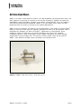
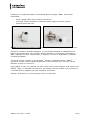
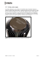
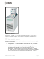
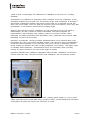
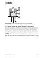
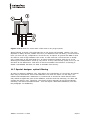
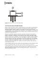
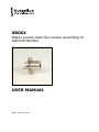
SBG01
Water cooled heat flux sensor according to
Schmidt Boelter
USER MANUAL
sbg01 manual v1208
SB G0 1 m a nu a l v 1 20 8
2/42
Contents
Contents
List of symbols
Introduction
1.
Gene ral Theory
1.1
General heat flux sensor theory
1.2
Considerations when using a heat flux sensor
1.3
Cooling water supply
1.4
Using uncooled sensors
2.
Error sources
2.1
Non-linearity
2.2
Errors due to convection
2.3
Radiation balance
3.
Application in F ire testing
3.1
Ignitability test ISO 4557
3.2
Spread of flame test: ISO 5658
3.3
Heat release, smoke production and mass loss: ISO 5660 and ISO 17554
4.
Specifications
5.
Short user guide
6.
Putting SBG01 into operation
7.
Installation of SBG01
8.
Maintenance of SBG01
8.1
Recoating SBG01
9.
Re quireme nts for amplification/ data ac quisition
10.
Electrical connection of SBG01
11.
Appendices
11.1 Appendix on cable extension for SBG01
11.2 Appendix on trouble shooting
11.3 Appendix on heat flux sensor calibration
11.4 Appendix on typical and allowable levels
11.5 Special designs: conical receivers
11.6 Special designs: air purging /avoiding condensation
11.7 Special designs: optical filtering
11.8 Gardon versus Schmidt Boelter
11.9 Appendix on (future) standard ISO TS 14934 Fire tests-calibration of heat flux
meters
11.10 Appendix on def ining new sensors
11.11 Appendix on heat flux versus the view factor
11.12 CE declaration of conformity
SB G0 1 m a nu a l v 1 20 8
3
4
5
8
8
8
10
11
13
13
13
15
17
17
17
18
19
21
22
23
24
24
26
27
29
29
29
30
32
33
34
35
36
37
39
39
40
3/42
List of symbols
Heat flux
Voltage output
SBG01 sensitivity
Time
Surface area
Electrical resistance
Temperature
Temperature dependence
Flow
Heat transfer coefficient
Wind speed

V
Es en
t
A
Re
T
TD
F
Ctr
Vwind
W m- 2
V
V/Wm- 2
s
m2

K
%/K
m3 /s
W/(m2 K)
m/s
Subscripts
Property of the sensor
Property of convective source
Property during calibration, at full scale
Property radiant source
Property at the soil surface
Incoming
Outgoing
True, as opposed to measured
SB G0 1 m a nu a l v 1 20 8
sen
conv
cal
rad
surf
in
out
true
4/42
Introduction
SBG01 is a water-cooled heat flux sensor. The ISO standards call this heat flux meter. Its
main purpose is the study of reaction to fire and fire resistance, applied for instance in
flammability tests and smoke chamber tests. SBG01 measurements are in accordanc e
with various ASTM and ISO standards. SBG01 is on the market since 2008, and has
rapidly become the sensor of choice for fire testing laboratories.
SBG01 serves to measure the heat flux of fire and flames in the range up to 200 kW/m2 .
Heat flux sensors of this type are originally designed to work in an environment that is
dominated by radiation (so above 50 kW/m2 ). Application in environments lower
irradiance levels and with much convection should be done with care. Working
completely passive, using a thermopile sensor, SBG01 generates an output voltage
proportional to the incoming flux. The sensor is water cooled. There are 6 types of
SBG01, with different working range, sensitivity and response time.
Figure 1 SBG01 Heat flux sensor / heat flux meter
SB G0 1 m a nu a l v 1 20 8
5/42
Comparing to traditional Gardon and Schmidt Boelter gauges, SBG01 has several
advantages:
-
water cooling tubes with increased robustness
increased scratch resistance of absorber paint (slightly lowered surface)
practical protection cap
Figure 2 protecting the sensing surface is convenient with the practical protection cap.
Hukseflux provides traceable calibration, our secondary standard is calibrated at the
Statens Provningsanstalt (SP), Sweden and by definition is thereby also traceable to
NIST. Hukseflux is not a “certified lab”; if required, the user is responsible to maintain
certified traceability.
The actual sensor in SBG01 is a thermopile. Working completely passive, SBG01
generates a small output voltage proportional to the local heat flux. This flux can be
radiative as well as convective.
Using SBG01 is easy. For readout one only needs an accurate voltmeter that works in the
millivolt range. To calculate the heat flux, the voltage must be divided by the sensitivity;
a constant that is supplied with each individual instrument.
Cooling can be done by connecting the sensor to tap water.
SB G0 1 m a nu a l v 1 20 8
6/42
Figure 3 SBG01 from top to bottom: 3D view, side view, top view, Dimensions in mm.
Coated sensing element (1), water cooling tube (2), Outer diameter tube: 4,2 mm, signal
cable (3). Standard cable length is 2 m.
SB G0 1 m a nu a l v 1 20 8
7/42
1. General Theory
1.1
General heat flux sensor theory
A heat flux meter is a measurement instrument with which the heat flux from the
environment to the sensor at the location (and in the plane of) the absorber can be
measured. As pointed out in the introduction, in most cases the main contribution to this
heat flux will be the irradiance as received from the so-called source. In a normal
situation the field of view of the sensor is assumed to be 180°, and the surface is
assumed to behave as a perfect blackbody, both regarding the spectral characteristics
and the directional response.
As in most heat flux sensors, the actual sensor in SBG01 is a thermopile. This thermopile
measures the differential temperature across a small plastic body inside SBG01. Working
completely passive, it generates a small output voltage that is proportional to the
differential temperature that powers the heat flux travelling through it. (Heat flux is
proportional to the differential temperature divided by the local thermal conductivity of
the heat flux sensor). This sensor is coated black, in order to have a flat spectral
sensitivity. It is silently assumed that sensitivity does not depend on wavelength over the
spectral range of the radiating sources, commonly analysed. Also deviations from the
ideal directional response characteristics can normally be neglected.
The sensor is mounted on a heat sink, which is water-cooled. The total assembly is able
to cope with high radiation levels; up to 200 kW/m2 .
Assuming that the heat flux is steady, that the thermal conductivity of the body is
constant and that the sensor has negligible influence on the thermal flow pattern, the
signal of SBG01 is proportional to the local heat flux in Watt per square meter.
Using SBG01 is easy. For readout one only needs an accurate voltmeter that works in the
millivolt range. To convert the measured voltage V s en to a heat flux , the voltage must
be divided by the sensitivity Es en, a constant that is supplied wit h each individual sensor.
 = Vs en / Es en
1.1.1
NOTE: see also paragraph 2.3 for lower flux levels.
SBG01 complies with the CE directives.
1.2
Considerations when using a heat flux sensor
SBG01 sensors are used for many purposes; the most common application is in various
types of "fire testing" (or reaction-to-fire testing). These tests involve spread of fire,
flammability testing, smoke release and many other aspects related to fire.
SB G0 1 m a nu a l v 1 20 8
8/42
It is important to understand the limitations of what Hukseflux does and does not supply.
This is particularly relevant to customers working in (fire) testing, where testing is used
as part of certification and subject to legal liability. The main conclusions are that:

The user must always let his reference sensor or reference sensors be calibrated
at a "reference institute". At present these are: NIST, SP and LNE.

Working along the (future) ISO standards, the user must buy at least 4 sensors of
which 3 are “secondary standard”, and meant as internal references, and one to
work with (“working standard”). An SBG01 heat flux meter could be calibrated as
secondary standard. Below a summary of considerations.
1 The SBG01 sensor specifications are such that in principle the sensor may be used for
certain types of fire testing, flammability testing etc. However, for performing a test "by
the book" it is not sufficient to have a sensor with the right specifications. The calibration
of the sensor, as well as the procedures followed by the user for quality assurance (to
verify stable behaviour) need to be implemented according to the applicable standards.
It is essential to realise that the measurement uncertainty is a function of:

Sensor properties

Calibration traceability of and quality assurance of the local reference at the
customer

Quality assurance of calibration of SBG field sensors or "working standards" in day
to day measurements

Measurement-related errors, for instance caused by convection
2 The calibration as performed at Hukseflux during manufacturing (factory calibration) of
the SBG sensors typically is NOT sufficient to be used immediately in certified fire related
experiments. The formal status of the c alibration is “against a working standard”
according to the procedure ISO 14934-3. Also when working within a certified laboratory,
for instance according to ISO 17025, or even according to ISO 9000, the customer will
have to send its calibration references to a certified calibration lab (this may be NIST in
the USA, LNF in France or SP in Sweden). Hukseflux is NOT formally certified to carry out
calibrations. Hukseflux does believe that its calibrations are within the specified accuracy,
but from a formal standardisation point of view this is not sufficient. Because Hukseflux is
not a certified laboratory, SBG01 sensors as delivered by Hukseflux are not 'secondary
standard', nor 'working standard' according to ISO TS 14934-4. As a source for primary
calibration (resulting in a secondary standard instrument), Hukseflux recommends SP in
Sweden. As an alternative source for calibration, NIST in the USA can be contacted.
3. If the user wants to follow the (future) ISO TS 14934-4 standard (for details see
appendix), the user should purchase at least 4 (four!) sensors: 3 (three) to be calibrated
by a laboratory as 'secondary standard' and 1 (one) to be used as 'working standard'.
See section 'ISO TS 14934-4 Fire tests-calibration of heat flux meters' for additional
information.
SB G0 1 m a nu a l v 1 20 8
9/42
1.3
Cooling water supply
For normal applications in fire research, the standard 3 bars of tap water supply are
sufficient for operating heat flux meters. In case of extremely high fluxes, which are not
relevant to SBG01 (above 2500 kW/m2 ), additional pressure may be necessary. As water
has a very high heat capacity; for 1 inch (25.4 mm) diameter sensors a water supply of
30 l/hr or 0.01 l/s is sufficient to carry away all the generated heat with a temperature
rise of less than 10 degrees C. (safety factor of 4). If it is impractical to use tap water,
for passive closed circuit cooling of SBG01, Hukseflux successfully employed the Zalman
reserator. Closed circuit water cooling with convective heat exchanger.
Figure 1.3.1 close up of the convective cooling of the reserator
SB G0 1 m a nu a l v 1 20 8
10/42
Figure 1.3.2 Julabo F12
An alternative possibility is to use a large vessel filled with water or coolers such as
supplied by the Julabo company, such as model F12 refrigerated / heated circulator
1.4
Using uncooled sensors
In some cases a non-cooled SBG01 may be used (so not connected to the water supply).
This can be considered if:
1. the measurement is so short that SBG01 cannot significantly heat up; typically
this requirement is fulfilled in case the time is less than 1 second;
2. the flux is so low that SBG01 cannot significantly heat up; typically this
requirement is fulfilled in case fluxes are lower than 1 kW/m2 . In this case it is
relevant to consider that SBG01 is very inaccurate anyway in low flux
measurements because typically the convective flux starts playing a significant
role. (please note that in general Hukseflux discourage measurements with SBG01
below 10 kW/m2 because of low expectations of the measurement accuracy)
SB G0 1 m a nu a l v 1 20 8
11/42
3. there is a large heat sink (for instance a block of aluminium or melting stearin)
attached to SBG01
4. any combination of 1, 2 and 3.
In all cases it is recommended:
5. to perform an experiment with similar temperature rise versus time, but no heat
flux to the sensor, to get an order of magnitude of the offset signal that is
produced by the SBG01 just due to the thermal shock (please note that a thermal
shock -rise of temperature- of the housing goes together with a heat flux to the
sensor, and thus a negative offset.)
6. to see that temperature of the sensor remains below 70 degrees C (the limit of
materials is 150 degrees C, but the centre of the sensor get hotter in case of
incoming heat flux)
7. to minimize the exposed surfaces by adding heat shields and insulation
8.
to try and calculate temperature rise before experimenting; the SBG01 weight is
around 110 grams of metal, so it has a heat capacity of 44J/K (heat capacity is
around 400J/(kgK).
9. In any case add as much mass as possible and shield the sensor from any
radiation not necessary for the measurement.
Example calculation: at 100 kW/m2 and a surface area of 5/1000 m2 , the incoming
energy is 50 W, which results in 1.2 K/s temperature rise. Starting at 20 degrees C, a
measurement time of 40 s is feasible.
SB G0 1 m a nu a l v 1 20 8
12/42
2. Error sources
Measurements with heat flux sensors are subject to errors. The basic calibration is
performed at full scale (depending on the type, this is 5, 10, 20, 50, 100 or 200 kW/m2 ).
The initial calibration accuracy is +/- 3%. Added to this initial error, the most significant
error sources are non-linearity, convection, and the radiation balance
2.1
Non-linearity
The SBG01 is calibrated at the full range, however with a minimum of 20 kW/m2 and a
maximum at 100 kW/m2 . When measuring at a fraction of the full range, the sensor is
expected to have an output V that varies linearly with the heat flux. This is only
approximately true. The deviation from ideal behaviour is captured in the so -called nonlinearity. This specification expresses the maximum deviation from ideal behaviour. The
non-linearity is expressed in percentage of the full scale heat flux. Non-linearity errors
can be quite large. The main conclusion is:If this is possible, heat flux sensors should be
used at flux levels higher than 50% of the full scale range.
c al = Vs en, c al / Es en, c al
2.1.1
With c al the full scale heat flux, as used during calibration.
During a measurement in practice:
 = Vs en / Es en, c al
2.1.2
or
 = ( Vs en / Vs en, c al) ) c al
2.1.3
The non-linearity, NL, is expressed as:
NL = (true -  )/ c al
2.1.4
With true , the true heat flux, and thus true -  the measurement error.
It should be noted that the non-linearity is allowing for quite large relative error margins
at lower flux ranges. For the 200 kW/m2 model, the +/- 2% allows a +/- 4 kW/m2 error.
When measuring with the same sensors at 20 kW/m2 , this is an error of +/ - 20%.
2.2
Errors due to convection
In most applications, the purpose of the heat flux measurement is to measure radiant
energy. Assuming that this is the purpose, it is a problem that heat flux sensors like
SBG01 are sensitive both to convection and to radiation. In most cases the errors caused
by this, are simply accepted as part of the inaccuracy of the measurement. In order to
get some idea of orders of magnitude one can take a look at the following text. The main
conclusions are:
SB G0 1 m a nu a l v 1 20 8
13/42
1. in an outdoor environment, below 50 kW/m2 it is not realistic to claim accuracies
within +/- 15%. (including calibration uncertainty)
2. in fire related experiments one should make sure that either radiat ive fluxes are
high or that the convective heat transfer is low (the latter by reducing air
temperature or by reducing air speed). A typical fire related indoor experiment
should be radiation-dominated.
Convective air will create two errors:
1. the convective error: a positive and negative contribution to the heat flux,
depending on the difference between air temperature and sensor temperature.
Please note that, in case it is the purpose of the experiment to measure the local
convective plus radiative flux, t his is not a measurement error.
2. the sensitivity error: the local heat transfer coefficient will vary with air speed, so
with air speed the effective sensitivity for radiation will vary.
In buildings, under indoor conditions we can expect wind speeds of 1 m/s. Working
environments will 90% of the cases have wind speeds below 0.5 m/s. Under outdoor
conditions up to 30 m/s can be considered normal, with 90% of the cases below 15m/s.
A reasonable approximation of the heat transfer coefficient at moderate wind s peeds is
given by:
Ctr = 5 + 4 Vwind
2.2.1
With Ctr in W/(m2 K) and in Vwind m/s.
In fires, no heat transfer coefficient data are known, however, we are working with a
figure of 50 W/(m2 K). As a qualitative experiment we consider several cases; a heat
transfer coefficient of 10 and 50 W/(m2 K), three flux levels 10, 50 and 100 kW/m2 , 2
sensor thermal resistances of 1000 and 2000 W/(m2 K), and two air temperatures of 400
and 20 degrees C, all at 10 degrees C sensor body temperature.
SB G0 1 m a nu a l v 1 20 8
14/42
Table 2.2.1 convec tion related error estimates in different environments. Convective
error is estimated, under the assumption that the purpose is to measure the radiative
flux rad, and that measurement of conv is undesired. The sensitivity error is estimated
by taking the ratio of the two thermal resistances Ctr and R sen.
Rsen
Tair
Tsen
 conv
CONVECTIVE
ERROR
SENSITIVITY
ERROR
kW/m2 W/(m2K)
W/(m2K)
deg C
deg C
kW/m2
%
%
10
50
2000
20
15
0.5
5%
3%
50
50
2000
20
35
0.5
1%
3%
100
50
2000
20
60
0.5
1%
3%
10
10
2000
20
15
0.1
1%
1%
50
10
2000
20
35
0.1
0%
1%
100
10
2000
20
60
0.1
0%
1%
10
50
1000
20
20
0.5
5%
5%
50
50
1000
20
60
0.5
1%
5%
100
50
1000
20
110
0.5
1%
5%
10
10
1000
20
20
0.1
1%
1%
50
10
1000
20
60
0.1
0%
1%
100
10
1000
20
110
0.1
0%
1%
10
50
2000
400
15
19.5
195%
3%
50
50
2000
400
35
19.5
39%
3%
100
50
2000
400
60
19.5
20%
3%
10
10
2000
400
15
3.9
39%
1%
50
10
2000
400
35
3.9
8%
1%
100
10
2000
400
60
3.9
4%
1%
10
50
1000
400
20
19.5
195%
5%
50
50
1000
400
60
19.5
39%
5%
100
50
1000
400
110
19.5
20%
5%
10
10
1000
400
20
3.9
39%
1%
50
10
1000
400
60
3.9
8%
1%
100
10
1000
400
110
3.9
4%
1%
 rad
2.3
Ctr
Radiation balance
Also it should be realized that, calibrating using radiation, the output of a heat flux
sensor n fact is a radiation balance
SB G0 1 m a nu a l v 1 20 8
15/42
 = in - out
Where  is the heat flux in kW/m2 as measured by the heat flux sensor, in is the incident
heat flux in kW/m2 and out is the emitted heat flux in kW/m2 .
Taking radiative transport only:
4
in =  T
s ensor
out =  T
4
s ource
Where  is Boltzmann’s constant, 5.67 10- 8 W/m2 K4 , T s ensor is the sensor temperature
in K, assuming a blackbody absorber, and T s ource is the source temperature in K,
assuming a uniform source.
The heat flux out from the absorber of 20 degrees Celsius is around 0,420 kW/m2 . This
implies that in calibration where the sources are typically 800 degrees C and higher,
(which implies at full view angle, around 75 kW/m2 ) this contribution is usually
neglected. In these cases this forms only 0.6% of the total contribution. In case that
fluxes of less than 75 kW/m2 are measured with a sensor temperature of approximately
20 degrees, the resulting error will be larger than 0.6%. Concluding: At a level of 10
kW/m2 the error is around 5%, and at lower levels than 10 kW/m2 a correction for out
should be made.
SB G0 1 m a nu a l v 1 20 8
16/42
3. Application in Fire testing
In this chapter examples are given of the application of heat flux meters in standardized
test environments for fire testing. The text serves solely as illustrative, and for detailed
test procedures, the individual standards should be consulted.
If employed according to the directions of the standard, including proper calibration and
quality assurance procedures by the user, SBG01 is expected to be suitable for use.
Some FAA standards specifically mention the use of Gardon Gauges. See the appendix on
Gardon versus Schmidt Boelter.
3.1
Ignitability test ISO 4557
The specimen is exposed to 5 levels of incident heat flux (10, 20, 30, 40, 50 kW/m2 ) and
the ignition time under each incident heat flux level is measured. The levels of 30 and 40
are most common. A heat flux meter is attached to a non-combustible board which is
placed in the specimen position. The temperature of the cone heater is adjusted in order
to obtain the required incident heat flux to the specimen position. Gardon - or SchmidtBoelter type heat flux meters can both be used for the purpose. A heat flux meter with
working range of up to 100 kW/m2 should be used. Its absorber should be 10 mm in
diameter. The sensor should have 3% accuracy and 0.5% reproducibility.
3.2
Spread of flame test: ISO 5658
The distribution of incident heat flux in the plane of the specimen are prescribed in the
Table.
Table 3.2.1 ISO 5658, heat flux as a function of distance along the centre of the
specimen
DISTANCE (mm)
INCIDENT HEAT FLUX (kW/m2)
50
50.5
100
49.5
150
47.1
200
43.1
250
37.8
300
30.9
350
23.9
400
18.2
450
13.2
500
9,2
550
6.2
600
4.3
SB G0 1 m a nu a l v 1 20 8
17/42
650
3.1
700
2.2
750
1.5
In order to achieve repeatability with earlier testing, prior to the test itself the complete
system is adjusted. This is done by measurement of the heat flux at the fixed locations
using a heat flux meter inserted into holes in a non-combustible board (for example,
silicic acid calcium board with a density of about 800 kg/m3 ). The board is temporarily
put in place of the specimen and the gas supply to the heat source is adjusted in order to
get the prescribed distribution of heat flux. The area of the non-combustible board within
300 mm from the edge receiving lower heat flux is lowered by 10 mm in order to prevent
convective heat flux around the area. This is necessary because in that area the
convective flux is relatively high in comparison with the radiant heat flux. When no
measurement is done in a hole it, should be closed by plugs made of the specimen
material and with a minimum discontinuity of the surface area. Incident heat flux at X
location closest to the heat source is about 50 kW/m2 , enough to ignition to clothes and a
burn, so care should be taken when conducting the experiment.
3.3
Heat release, smoke production and mass loss: ISO 5660 and
ISO 17554
In this test the heat flux meter is used to verify the heat flux level at the location of the
specimen. A Schmidt-Boelter type heat flux meter with a working range of 0-100 kW/m2
should be used for adjusting the heat flux level. The most commonly used fluxes are 35
and 50 kW/m2 . An accuracy of 3% and a repeatability of 0.5% are required. The
stabilization time is 3 minutes. The diameter of the black paint on the absorber is a bout
12.5mm. It is important that the cooling water is flowing and the vulnerable black
coating on the absorber is handled with care. In order to maintain a stable reference,
calibration of the heat flux meter should be done on a daily basis. The absorber should
be positioned at the location of the central part of the specimen. If necessary the
specimen holder should be removed in order to be able to allow the sensor at that
particular location.
Other fire testing involving heat flux sensors
ISO 9705:1993 Fire tests — Full-scale room test for surface products
ISO 17431:2006 Fire tests-- Reduced-scale model box test
ISO 17385 series; Façade test
ISO 3008 Fire resistance of doors
ISO 5657:1997 Reaction to fire tests — Ignitability of building products using a radiant
heat source
ISO 5659-2:2006 Plastics — Smoke generation — Part 2: Determination of optical
density by a single-chamber test
ISO 14696:2009 Reaction-to-fire tests — Determination of fire and thermal parameters
of materials, products and assemblies using an intermediate-scale calorimeter (ICAL)
ISO 13785:2002 Reaction-to-fire tests for façades
ISO 9239-1:2002 Reaction to fire tests for floorings — Part 1: Determination of the
burning behaviour using a radiant heat source
SB G0 1 m a nu a l v 1 20 8
18/42
4. Specifications
SBG01 is a water-cooled heat flux sensor that measures the local heat flux perpendicular
to the sensor surface. It is normally used in combination with a suitable water supply and
a measurement system. The sensor is optimised to be used in high-flux, radiationdominated environments. There are 6 types of SBG01, calibrated at different working
ranges.
Table 4.1 List of SBG01 specifications.
SBG01 GENERAL SPECIFICATIONS
1
Specified measurements
Heat flux in W/m2 perpendicular to the sensor surface
2
Installation
See the product manual for recommendations, for normal
use the sensor must be connected to water supply.
3
Recommended number of
sensors
Fire research: at least 2 to have redundancy of the
measurement
4
CE requirements
SBG01 complies with CE directives
-2
5
Working ranges kWm
5, 10, 20, 50, 100, 200
6
Cooling water flow:
> 10 litre/hr, preferably 30 litres per hour @ 3 bar (normal
tap water)
SBG01 may be used uncooled at low flux levels or for short
durations.
7
Temperature range cooling
water:
5 to +30 oC
8
Cooling water supply
NOT SUPPLIED WITH THE SENSOR: Typically through 6 mm
outer diameter / 3 mm inner diameter silicone hose.
Hose may be interrupted by couplings.
(colder.com) type MCD1702 BODY 1/8 inch NPT+MCD4202
INSERT
9
Order Code:
SBG01/RANGE/ cable length
EXAMPLE: SBG01/ 200 / 2
SBG01 MEASUREMENT SPECIFICATIONS
10
Initial calibration accuracy
+/- 6 % (revised following ISO TS 14934)
11
Overall calibration uncertainty
statement according to ISO
Estimated to be within +/- 6 %, based on a standard
uncertainty multiplied by a coverage factor of k = 2,
providing a level of confidence of 95%.
NOTE: Application-related errors should be added to this
error.
SBG01 SENSOR SPECIFICATIONS
12
E sen (nominal)
exact value on calibration certificate
13
Output signal
Analog voltage
> 5 mV at working range
14
Maximum heat flux range
150% of working range
15
Response times:
Working range 5, 10 kW/m2:
Working range 20, 50 kW/m2:
SB G0 1 m a nu a l v 1 20 8
< 450 ms (63%)
< 250 ms (63%)
19/42
Working range 100, 200 kW/m2: < 200 ms (63%)
16
Temperature dependence TD
< +0.1%/ °C
17
Non stability
Unspecified, expected < 1% change per year under clean
conditions.
18
Required readout
1 differential voltage channel
19
Spectral range
to 50.000 nm
20
Field of view
180 degrees
21
Emissivity
> 0.95
22
Power required
Zero (passive sensor)
23
Resistance
25 Ohm (nominal) plus cable resistance
24
Required programming
 = Vsen/ E sen
25
Non-linearity
Within +/- 2% of full range
26
Cable length, diameter
2 meters, 3.1 mm diameter PTFE
27
Weight including 2 m cable,
transport dim.
0.2 kg
transport dimensions 9x17x23 (0.3 kg)
CALIBRATION
28
Calibration traceability
To primary standard level of SP, and also to NIST
(Hukseflux is not a certified laboratory)
29
Recalibration interval
Dependent on application, if possible every 2 years, see
appendix
30
Calibration status
Against “working standard” (ISO 14934)
OPTIONS
31
SB G0 1 m a nu a l v 1 20 8
Additional cable length x metres (add to 2m),
AC100 amplifier,
LI 19 hand held readout
20/42
5. Short user guide
Preferably one should read the introduction and first chapters to get familiarised with the
heat flux measurement and the related error sources. In any case the remarks about
error sources (Chapter 2) should be read.
IT is also useful to familiarise oneself with the ISO group of standards 14934.
The sensor should be installed following the directions of the next paragraphs. Essentially
this requires water supply, a data logger and control system capable of readout of
voltages, and capability to perform division of the measurement by the sensitivity.
The first step that is described in chapter 6 is and indoor test. The purpose of this test is
to see if the sensor works.
The second step is to make a final system set -up. This is strongly application dependent,
but it usually involves permanent installation of the sensor and connection to the
measurement system.
Directions for this can be found in chapters 7 to 10.
SB G0 1 m a nu a l v 1 20 8
21/42
6. Putting SBG01 into operation
It is recommended to test the sensor functionality by checking the impedance of the
sensor, and by checking if the sensor works, according to the following table: (estimated
time needed: 10 minutes).
Table 6.1 Checking the functionality of the sensor. The procedure offers a simple test to
get a better feeling how SBG01 works, and a check if the sensor is OK
1
Remove cap
Typically SBG01 is supplied with a plastic protection
cap. This should be removed.
2
Warning: during this part of the
test, please put the sensor in a
thermally quiet surrounding
because a sensor that
generates a significant signal
will disturb the measurement.
The typical impedance of the wiring is 0.1 ohm/m.
Typical impedance should be 1.5 ohm for the total
resistance of two wires (back and forth) of each 5
meters, plus the typical sensor impedance of 25 ohms.
Infinite indicates a broken circuit; zero indicates a short
circuit.
Check the impedance of the
sensor. Use a multimeter at the
100 ohms range. Measure at
the sensor output first with one
polarity, than reverse polarity.
Take the average value.
3
Connect to water supply
Typically a silicone hose of outer diameter 6 mm and
inner diameter 3 mm is used.
4
Check if the sensor reacts to
The thermopile should react by generating a millivolt
heat flux. Use a multimeter at
output signal.
the millivolt range. Measure at
the sensor output. Generate a
signal by putting the sensor in
front of a strong radiant source,
for instance a spotlight
The programming of data loggers is the responsibility of the user. Please
contact the supplier to see if directions for use with your system are available.
SB G0 1 m a nu a l v 1 20 8
22/42
7. Installation of SBG01
In general the heat flux sensor is expected to be located at the point where one wants to
measure the heat flux, typically aimed into the direction of the main heat source or flush
with the sample that is under testing.
In fire testing, installation methods of heat flux sensor into test equipment is usually
specified in the test standard.
In many cases holes are drilled in the specimen to accommodate the body of a heat flux
sensor.
It is recommended to mount the sensor in such a way that the transfer of heat to the
heat flux sensor body or flanges is as low as possible.
In general it is recommended to have the surface of the heat flux meter at the same
height as the surface or “flush with” of the specimen.
In case the surface of heat flux meter is on a same level of the surface of specimen, both
convective and radiative heat is measured. In case the surface of heat flux sensor
protrudes from the surface of the specimen, in particular when oriented vertically, the
convective heat flow on the specimen may not be correctly measured by the heat flux
sensor. If the heat flux sensor recesses from the surface of the specimen, the edge and
side wall of the hole of the specimen limit the field of view to the heat source and may
affect combustion behaviour. Recessed as well as protruded mounting should be done in
exceptional cases only, and be well documented.
In a large scale test for fire research, the incident heat flux to the specimen is sometimes
measured. In order to install a vertical type heat flux meter into a specimen, a hole shall
be made in the specimen through which the heat flux meter is inserted. In this case,
tubes for water supply and lead wires may be protected by the specimen. However, care
should be taken to avoid damage or mechanical stress to the sensor by collapse or
deformation of the specimen.
In case of permanent mounting, it is a possibility to mount the sensor in such a way that
the sensor surface is a little lower (say 3 mm) than the surrounding surface. In that case
the sensor surface can be protected by putting a plate over the sensor.
SB G0 1 m a nu a l v 1 20 8
23/42
8. Maintenance of SBG01
Once installed, SBG01 is essentially maintenance free. Usually errors in functionality will
appear as unreasonably large or small measured values.
In fire testing, sensors should be compared to a reference under a radiant source, before
and after testing. See appendix on calibration.
In case two sensors are mounted on one location the ratio of measurement results could
be monitored over time; this will give a clue if there is any instability. Typically long term
comparison of 2 sensors can serve as an alternative for re-calibration at the factory.
As a general rule, that a critical review of the measured data is the best form of
maintenance.
At regular intervals the quality of the cables can be checked.
During the use of heat flux meters, the colour of the absorber surface may change. This
might be caused by overheating, soot deposition, reactions of the coating with gasses
etc. In case of minor colour change, the heat flux meter may be used after cleaning the
surface, and recalibration. If the extent of colour c hange is large, or in case of the
coating letting loose, the surface shall be repainted in accordance with manufacturers
recommendations. When the absorber of a heat flux meter is repainted or substantially
cleaned, the heat flux meter shall be calibrated.
Re-painting in general should be done at the manufacturer.
In case of emergency one may decide to repaint the sensor by oneself. In general high
temperature black paints should be used. Suitable paints are generally found in the carsupply for coating c ar parts. Temperature resistance should be higher than 600 degrees.
(see next paragraph for more details)
8.1
Recoating SBG01
SBG01 sensor surface is covered with a specially developed "Hukseflux Black" paint with
a rough surface. This has excellent absorptance, good directional response and is
temperature resistant up to at least 120 degrees C. The painted surface is located just
0.2 mm retracted relative to the local metal front surface to offer protection against
scratching. The paint will survive light mec hanical force, but will not survive hard
scratching. It dissolves in alcohol and acetone, and does not withstand extended
operation in wet conditions.
In case the paint surface is scratched or damaged, the sensor surface will be exposed.
This surface is a polyimide plastic with an orange colour. The effect of a locally removed
black paint will be a reduction of the SBG01 sensitivity to radiation. There is no way of
estimating the magnitude of this reduction. Locally removed paint will not lead to
damage to the sensor.
To protect the paint, it is recommended to use the SBG01 cap to protect the sensor
surface whenever the sensor is not used.
SB G0 1 m a nu a l v 1 20 8
24/42
In case of a damaged paint layer, Hukseflux can recoat and recalibrate your sensor.
In case of emergency the user can re-paint the surface with a temperature resistant
paint "heat resistant paint" or “high temperature lacquer”. This must always be combined
with a re-calibration. The paint can be obtained as ready-to-use spray cans in car repair
shops. It is typically used to paint exhaust pipes and motors. The temperature resistance
is typically up to 500 degrees C. This paint can also be used to apply with a small brush
for small repairs of the sensor coating. When recoating the full sensors, the old coating
can be removed by using alcohol.
It should be noted that if the user decides to coat by himself, no more claims to warranty
can be made. Also recalibration is necessary after coating. Recalibration is the user's
responsibility. Since the paint type is different to the specially developed "Hukseflux
Black", directional response properties are no longer specified.
SB G0 1 m a nu a l v 1 20 8
25/42
9. Requirements for amplification/
data acquisition
Table 9.1 Requirements for data acquisition and amplification equipment.
1
Capability to measure microvolt Preferably: 5 microvolt accuracy
signals
Minimum requirement: 50 microvolt accuracy
(both across the entire expected temperature range of
the acquisition / amplification equipment)
In case of low amplifier accuracy it should be
considered either to put two sensors in series or to
purchase a pre-amplifier.
2
Capability for the data logger or To store data, and to perform division by the sensitivity
the software
to calculate the heat flux.
SB G0 1 m a nu a l v 1 20 8
26/42
10. Electrical connection of SBG01
In order to operate, SBG01 should be connected to a measurement and system as
described above. A typical connection is shown in table 10.1. SBG01 is a passive sensor
that does not need any power. Cables generally act as a source of distortion, by picking
up capacitive noise. It is a general recommendation to keep the distance between data
logger or amplifier and sensor as short as possible. For cable extension, see the appendix
on this subject.
Table 10.1 The electrical connection of SBG01. The sensor output usually is connected
to a differential voltage input.
WIRE
COLOUR
MEASUREMENT SYSTEM
1
Sensor output +
White
Voltage input +
2
Sensor output -
Black
Voltage input – or
(Analogue) ground
3
Shield
SB G0 1 m a nu a l v 1 20 8
(Analogue) ground
or Voltage input -
27/42
SB G0 1 m a nu a l v 1 20 8
28/42
11. Appendices
11.1 Appendix on cable extension for SBG01
SBG01 is equipped with one cable. It is a general recommendation to keep the distance
between data logger or amplifier and sensor as short as possible. Cables generally act as
a source of distortion, by picking up capacitive noise. SBG01 cable can however be
extended without any problem to 100 meters. If done properly, the sensor signal,
although small, will not significantly degrade because the sensor impedance is very low.
Cable and connection specifications are summarised below.
Table 11.1.1 Specifications for cable extension of SBG01.
1
Cable
2-wire shielded, copper core (at Hukseflux we use 3
wire shielded, of which we only use 2 per cable)
Cores cladded with PTFE (black and white)
2
Core resistance
0.1 /m or lower
3
Outer diameter
(preferred) 3.1 mm
4
Outer sheet
(preferred) PTFE (for good stability in high temperature
applications).
5
Connection
Either solder the new cable core and shield to the
original sensor cable, and make a waterproof
connection using cable shrink, or use gold plated
waterproof connectors. Preferably the shield should also
be extended.
11.2 Appendix on trouble shooting
This paragraph contains information that can be used to make a diagnosis whenever the
sensor does not func tion.
Table 11.2.1 Trouble shooting for SBG01
1
The sensor does not give any
signal
1 Measure the impedance across the sensor wires.
This check can be done even when the sensor is buried.
The resistance should be around 25 ohms (sensor
resistance) plus cable resistance (typically 0.1 ohm/m).
If it is closer to zero there is a short circuit (check the
wiring). If it is infinite, there is a broken contact (check
the wiring).
2 Check if the sensor reacts to an enforced heat flux. In
order enforce a flux, it is suggested to connect the
sensor to water supply, and use a spotlight as radiant
source.
3 Check the data acquisition by applying a mV source
to it in the 1 mV range.
2
The sensor signal is unrealistically high or low.
1 Check if the right calibration factor is entered into the
algorithm. Please note that each sensor has its own
individual calibration factor.
SB G0 1 m a nu a l v 1 20 8
29/42
2 Check if the voltage reading is divided by the
calibration factor by review of the algorithm.
3 Check if the mounting of the sensor still is in good
order.
4 Check the condition of the leads at the logger.
5 Check the cabling condition looking for cable breaks.
6 Check the data acquisition by applying a mV source
to it in the 1 mV range.
7 check if the sensor front surface is still black. If not
send a picture to the supplier and consider recoating.
3
The sensor signal shows
unexpected variations
1 Check the presence of strong sources of
electromagnetic radiation (radar, radio etc.)
2 Check the condition of the shielding.
3 Check the condition of the sensor cable.
11.3 Appendix on heat flux sensor calibration
The sensitivity Es en of a Heat Flux Sensor is defined as the output Vs en for each Watt per
square meter heat flowing through it, in a stationary transversal heat flow.
Most laboratories will obtain a set of (typically 3) “secondary standard” heat flux meters
from one of the laboratories that are designated to perform this secondary calibration. At
present these laboratories are NIST (United States), SP (Sweden) and LNE (France).
Using this secondary standard, so-called “working standards” can be calibrated. These
working standards, in turn, will be used for day to day work. These working sensors
should be calibrated before and if possible after every experiment.
If considered necessary it is possible to use one step in between the secondary standard
and the working standard. This is called the laboratory standard.
Working standards used in fire tests shall be calibrated by comparison with secondary
standard or laboratory standard heat flux meters. The method of calibration of working
standards using a secondary standard is given in ISO 14934-3. The method of calibration
of laboratory standards is the same.
Normal calibration by SP and NIST can be performed up to 100 kW/m2 . Above this
extrapolation can be used.
The calibration reference conditions for SBG01 calibration at Hukseflux are:


Temperature: 10 °C
Heat Flux: full working range with a minimum of 20 kW/m2 .
Previously Hukseflux has specified its calibration uncertainty as +/- 3%. This statement
has been revised to +/- 6%. The secondary standard at Hukseflux is taken to be +/- 4%,
and there is 2% reserved for uncertainty of transfer. The calibration procedure at
Hukseflux involves comparison under a radiant source to a secondary standard Schmidt
Boelter gauge, which has been calibrated under exposure to a radiant source. The
temperature of this radiant source and thus the calibration is calibration is traceable to a
NIST temperature standard. The new ISO standards ISO/TS 14934-1:2002 and ISO
SB G0 1 m a nu a l v 1 20 8
30/42
14934-3:2006 would qualify this calibration as calibration at the level of a "working
standard".
At Hukseflux the calibration is performed under a radiant source by comparison to the
secondary standard at one point only, the working range, with a minimum of 20 kW/m2 ,
and a linear relationship between the signal and the heat flux is assumed around this
point. One of the major errors for heat flux sensors is their non-linearity; this is why ISO
recommends to use sensors around the full working range.
Working with heat flux sensors, calibration accuracy should not be seen as equal to
measurement accuracy. Heat flux sensors like SBG01 have been designed for
measurements with extremely high radiative (and not convective) fluxes. When
measuring at radiant intensities of 50 kW/m2and lower, significant errors can be made
depending on the local convection.
Hukseflux recommends checking working standards before every test and after every
test against the user’s secondary standard sensors. The reason for this recommendation
is that the test environment is very extreme, and there is a risk of damaging sensors
during testing (for instance by water cooling temporarily not working). This might result
in unstable sensor behaviour. This behaviour does not necessarily show up during
testing. If it goes unnoticed, the test results might be invalid.
Hukseflux manufactures calibration equipment that will make comparison to reference
sensors relatively easy. The picture shows CU02 calibration unit for heat flux sensors.
Figure 11.3.1 Picture of calibration unit CU02, showing water supply (in / out), power
supply and heat source (1250 Watt lamp, housing in blue). At the background the watercooled plate on which the sensors are mounted, is visible
SB G0 1 m a nu a l v 1 20 8
31/42
11.4 Appendix on typical and allowable levels
An indication of allowable heat flux levels for personnel and equipment can be found
below.
Table 11.4.1 Allowable heat flux levels in industrial environments
Btu/Hr Ft2
kW/m2
1
Equipment
3000
9.5
2
Human: Run
2000
6.3
3
Human: Walk
1500
4.7
4
Human: Work (static)
500
1.6
Table 11.4.2 Typical ranges of heat flux levels, from ISO
kW/m2
COMMENT
1
300
Maximum level in a fully developed fire
2
200 to 100
Incident heat flux on the wall in a developed fire enclosure
3
about 100
Radiation from burning house
4
about 30
Causing ignition of tree
5
20 to 10
Causing ignition of timber
6
about 7 or 8
Lowest level for causing ignition of a timber wall under a pilot
flame
7
about 4
Lowest level for causing a burn
8
about 2,5
Highest level for people to endure
9
1,5
Solar constant, maximum level of solar irradiance
Table 11.4.3 Irradiated heat flux versus blackbody source temperature
kW/m2
BLACKBODY Deg C
1
0.4
10
2
20
500
3
60
750
4
150
1000
5
200
1100
6
266
1200
The SBG heat flux sensor range is designed for operation in environments where the
radiant flux is the main source of heat. In most fire-related conditions this is the case.
Although the heat flux received by the sensor might also be related to high temperature
gasses, it is very difficult to transfer heat from the gas to the sensor. The heat transfer
by radiation is far more efficient .
SB G0 1 m a nu a l v 1 20 8
32/42
The question whether a sensor can or cannot be used in a certain environment can be
answered by calculation of the heat flux of the environment to the sensor. The starting
point is the sensor cooling water temperature, which is assumed to be anywhere
between 10 and 30 degrees C. The heat flux between the sensor and the environment is
determined by the radiant flux and the convective flux. In 90 % of the cases the radiant
flux dominates, and the convective flux can be ignored. In these cases the calculatio n is
simple; if the radiative flux is within the range of the sensor, the sensor will survive. To
estimate the maximum radiant flux: take the source temperature in degrees C, and
calculate the blackbody emission:
(Tsource -273)E+4 (5.67 10 E-8). Assuming a source filling the complete field of view of
a sensor, this is around 20 kW/m2 for 500 degrees C radiant source temperature, 60
kW/m2 for 750 deg C, 150 kW/m2 for 1000 deg C and 200 kW/m2 for 1100 deg C. For
fire related experiments, the estimated source temperatures are typically higher than
750 degrees C.
Convective flux levels can be estimated if we know the local heat transfer coefficients,
which are related to local convection or "gas speed". In most fire experiments the heat
flux by convection will be low; typical worst case transfer coefficients in the order of 20
W/m2 K; for instance at 750 degrees C gas temperature leading to a flux of within 15
kW/m2 , compared to the 60 kW/m2 by radiation. (so just 25%).
Only in cases of forced convection (jet impingement ovens) heat transfer by convection
becomes significant.
In case there is no forced convection, Hukseflux suggests using the source temperature
as a worst-case approximation and to estimate the maximum radiant flux take the
source temperature in degrees C, and calculate the blackbody emission (Tsource 273)E+4 (5.67 10 E- 8 ). A sensor with a proper working range can be chosen from that
analysis. In case there is forced convection, Hukseflux should receive an analysis of the
situation, including local gas temperature estimates and if possible gas speed or transfer
coefficients.
11.5 Special designs: conical receivers
Conical receivers are sometimes used for creating a sensor that is sensitive to radiative
flux only. The conical receiver has a reflecting interior (usually gold plating). This
configuration is used to keep the absorber free of the influence of convection. Heat flux
sensors with conical receivers are often used in flame research and are often equipped
with air purging to keep the reflector free of soot.
SB G0 1 m a nu a l v 1 20 8
33/42
Figure 11.5.1 a conical receiver that can be put in front of the absorber
11.6 Special designs: air purging /avoiding condensation
Air purging may be used in combination with a heat flux meter. This is particularly useful
when extensive amount of smoke or soot is expected during the experiment. Air purge
systems serve to prevent the smoke particles from accumulating onto the absorber of
the heat flux meter and also serve to avoid water condensation on the water-cooled
sensor (gasses from a fire are possibly saturated with water which will condensate on a
cold surface). It should be noted that purged air may affect the combustion and heat
transfer around the heat flux meter. Air purged sensors will sometimes require dedicated
calibration.
NOTE: many users build their own dedicated air-purging system around a sensor. This is
often more practical than using a system supplied by the manufacturer of the heat flux
sensor.
SB G0 1 m a nu a l v 1 20 8
34/42
Figure 11.6.1 Heat flux meter with a filter and an air purge system
When flushing a sensor, the total heat flux to the sensor will possibly change. The error
depends on many factors; radiant flux level (so radiation from the flame), convective flux
level (so from hot air), temperature of the hot air/ air speed. In general the SBG is most
accurate in case of high radiative flux levels. In that case the convective flux is usually
only a small part of the total heat flux. In these situations flushing with dry air is not
affecting the measurement result by very much. In any case the only proo f is to try it out
and look at the differences. This kind of check to estimate the influence of flushing is
almost unavoidable because it is hard to estimate from theory.
11.7 Special designs: optical filtering
In order to measure radiation only, and reduce the contribution of convection, an optical
filter may be attached in front of the absorber of a heat flux meter. In this way a so called total hemispherical radiometer is constructed. It should be noted that the filter
may absorb a significant part of the radiation, and also that the mounting of a filter will
change the field of view. Therefore, the choice of filter material as well as mechanical
mounting will affect the measurement. This will require dedicated calibration (see also
the paragraph on calibration).
SB G0 1 m a nu a l v 1 20 8
35/42
Figure 11.7.1 Heat Flux meter with optical filter
11.8 Gardon versus Schmidt Boelter
Gardon gauges are heat flux meters, typically identical in outer shape to Schmidt Boelter
gauges, using a different sensor construction. The distinction between Gardon gauges
and Schmidt Boelter gauges in general is not justified. Both are heat flux sensors,
designed to measure heat flux. Neither type is subject to a formal system of classification
or standardisation. In fire testing the only requirement is that calibration is traceable to a
certified laboratory and be performed at the working range, so that there should not be a
preference for using either one.
Although the measured quantity is the same, the sensor technology used in Gardon
gauges is different to compared to that in Schmidt Boelter gauges. The Gardon gauge
employs a thermopile consisting of a two joints only, while the Schmidt Boelter gauge
employs a multi-junction thermopile. The two-joint design of a Gardon Gauge is typically
made by using a nickel metal foil over a hole, and making a copper joint at the edge of
the foil as well as in the centre. This results in an all-metal construction. The advantage
of Gardon design is that, taking small diameter foils, it can handle larger flux levels than
the more complicated Schmidt Boelter design. The Schmidt Boelter design has the
advantage that it can be made more sensitive (at the same response time) and that it
can be made more linear.
A typical Gardon gauge will reach a higher foil centre temperature than a Schmidt Boelter
gauge at full specified range. This may result in different reaction to convection.
A typical Gardon gauge, because of its higher expected centre temperature will be coated
with a high temperature black paint, that will typically have a different and less ideal
directional response compared to that of a Schmidt Boelter gauge. This may lead to a
different measurement result.
SB G0 1 m a nu a l v 1 20 8
36/42
In a Gardon Gauge the sensor is electrically connected to the water supply and the
sensor housing. This may lead to grounding errors. In Schmidt Boelter designs the
sensor is electrically insulated.
11.9 Appendix on (future) standard ISO TS 14934 Fire testscalibration of heat flux meters
Heat flux sensors (officially “heat flux meters”) like SBG are nowadays subject to
standardization according to ISO TS 14934 “Reaction-to-Fire tests-calibration of heat flux
meters”. This standard will also be adopted by ASME.
In case a user wishes to perform certified testing or works in an ISO certified
organisation, the following is relevant:
This standard has 4 parts
1.
2.
3.
4.
General principles (Technical Specification)
Primary calibration methods
Secondary calibration method
Guidance on use of heat flux sensors (Technical Specification)
The most important practical consequences of the standards are:
-
the need to have local reference sensors calibrated at a “certified calibration
institute”.
the need to work with a sensor closely around the area of calibration.
the need, to have 3 "secondary standard" instruments for calibration of the
"working standards" (these are the instruments used for day to day work). At
Hukseflux this is identical to the sensor "range" as specified for the particular
sensor (Working ranges kW/m2 : 5, 10, 20, 50, 100, and 200) This need is not
clearly motivated in the standard. Hukseflux assumes the reason is as follows: at
every test there is a certain risk that the working standard is damaged in such a
way that the sensor might become unstable. This is a consequence of the fact that
the sensor is operating under unfavourable conditions (basically exposed to
flames), and the fact that water cooling might temporarily fall away. The
assumption made in the standard is that working standards are compared to a
local secondary standard before every test!
Some text from the standards:
Part 3 Secondary calibration method
Annex D (informative) Procedure recommended for maintenance of a secondary standard
of irradiance at a test laboratory
D.1 This annex outlines the procedure by which a test laboratory can maintain a reliable
secondary standard of irradiance. It is founded on the relative stability of sensitivity of
heat flux meters which are reserved entirely for calibration and inter-comparison
purposes and are never subjected to the rougher conditions of measurement in fire tests
SB G0 1 m a nu a l v 1 20 8
37/42
and experiments. Although the absolute determination of irradiance is a complex and
time-consuming procedure, the maintenance of calibration of secondary -standard
instruments is generally more straightforward.
D.2 The first step is to designate three heat flux meters (A, B, C) as secondary-standard
instruments to be reserved henceforth solely for calibration work. These are usually
commercially available Schmidt -Boelter measurement-type (thermopile) or Gardon
measurement type (foil) heat flux meters. These can either be new instruments
purchased specially, or instruments that have been used in the test laboratory but have
not been abused. In some cases, records of calibration can indicate certain instruments
as having a stable sensitivity over a period of years and such instruments are especially
suitable. The purchase of new instruments does not automatically ensure good stability
of sensitivity, although on the whole new instruments are likely to be satisfactory.
Part 4 Guidance on the use of heat flux meters
Introduction: in many practical situations in fire testing, the contribution due to
convection to the sensing surface of the instrument can amount to 25% of the radiant
flux. Therefore it is necessary to control this part.
6.2.1 Evaluating the working and calibration range
Excessive incident heat flux to a heat flux meter beyond its working range may cause
destruction of the heat flux meter. On the other hand, the use of heat flux meters to
measure at very low levels of heat flux (in relation to the working/c alibration range of a
heat flux meter) may cause large inaccuracies and errors. Therefore, the working range,
as well as the calibration range of the heat flux meter, should match the conditions of the
intended measurement.
8 Calibration
8.1 Secondary standard heat flux meter
A secondary standard heat flux meter, which has been calibrated in a laboratory that is
designated to perform this secondary calibration in accordance with ISO 14934-3, shall
be obtained in order to calibrate heat flux meters to be used in a laboratory. It is
recommended to prepare at least three secondary standard heat flux meters, which are
calibrated in accordance with ISO 14934-3. It is useful to conduct comparison calibration
between these secondary standard heat flux meters, so t hat a secondary standard heat
flux meter which gives wrong measurements can be found, assuming that the other two
are in order.
8.2 Working standard heat flux meters
Working heat flux meters to be used in fire tests should be calibrated by comparison with
the secondary standard heat flux meters following the method specified in ISO 14934-3.
8.3 Frequency of calibration
SB G0 1 m a nu a l v 1 20 8
38/42
Fire test standards may specify the interval of calibration of the working heat flux meter.
If there is no specification in the intended fire test standard, it is recommended to use
ISO 5660-1:2002, 10.3.1 for this purpose.
Part 1 General principles
ISO 14934-1 Uncertainty calculation
The accuracy of calibration of the working-standard heat flux meter depends on the
accuracy of calibration of the secondary-standard heat flux meter and also on the
accuracy with which the inter-comparison can be made. The latter depends both on the
accuracy of positioning of the working-standard heat flux meter in relation to the
secondary-standard heat flux meter and on the statistical errors due to averaging,
combining or comparing sets of data that, because of random processes such as physical
perturbations and reading errors, exhibit some variation. Establishing confidence limits
for the calibration of secondary-standard heat flux meters is the subject of several ongoing investigations (HFCAL and FORUM). In the absence of new data, an uncertainty of
better than ± 6 % (95 % confidence limit) is a conservative estimate.
11.10
Appendix on defining new sensors
In case new sensors need to be designed, please consider:
-
sensitivity (please state incoming level of flux, and nature (we assume solar
radiation?))
spectral response (should we match the colour to the colour of a sample? or
should we make a black surface)
angular response (a rough black paint with a perfect cosine response, or
something more reflective)
heat sink (is your object metal of otherwise, in other words, can the sensor loose
its heat input to your object)
calibration: any special requirements for instance: should we perform this under
non-vacuum or can you do this in vacuum.
response time (is response time relevant to your experiment?)
numbers: what number of sensors is required
delivery time: what delivery time is required
11.11
Appendix on heat flux versus the view factor
If an SBG01 is facing a source with limited dimensions, t he incident heat flux will become
dependent on the degree to which t he sensor is exposed to the source. In optical terms
there is a variable that defines this relationship for every distance, orientation and
surface shape. This is the so-called view factor.
http://en.wikipedia.org/wiki/View_factor
SB G0 1 m a nu a l v 1 20 8
39/42
11.12
CE declaration of conformity
We
of
Hukseflux Thermal Sensors
Elektronicaweg 25
2628 XG Delft
The Netherlands
in accordance with the following Directive:
2004/108/EC
The Electromagnetic Compatibility Directive
hereby declare that:
Equipment:
Type:
heat flux meter
SBG01
is in conformity with the applicable requirements of the following documents
Emission:
Immunity:
Emission:
Emission:
EN
EN
EN
EN
61326-1 (2006)
61326-1 (2006)
61000-3-2 (2006)
61000-3-3 (1995) + A1 (2001) + A2 (2005)
I hereby declare that the equipment named above has been designed to comply
with the relevant sections of the above referenced specifications and is in
accordance with the requirements of the Directive.
Signed
C.J. van den Bos
Director
Delft
6 September 2010
SB G0 1 m a nu a l v 1 20 8
40/42
SB G0 1 m a nu a l v 1 20 8
41/42
© Hukseflux Thermal Sensors B.V., 2011
www.hukseflux.com
Hukseflux Thermal Sensors B.V. reserves the right to change and/or alter specifications without notice.