Download RUMD tutorial

6
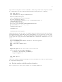
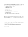
sim = rumdSimulation("start.xyz.gz")
Here sim is an arbitrary name we choose for the object. Next we choose an NVT integrator,
giving the time-step and temperature:
itg = IntegratorNVT(timeStep=0.0025, targetTemperature=1.0)
Having an integrator object, we need to connect it to the simulation:
sim.SetIntegrator(itg)
Next we need to choose the potential. For 12-6 Lennard-Jones we create a potential object,
giving it the name pot, as follows:
pot = Pot_LJ_12_6(cutoff_method=ShiftedPotential)
The mandatory argument cutoff_method specifies how the cut-off of the pair-potential is to be
handled. It must be one of ShiftedPotential (the most common method, where the potential
is shifted to zero), ShiftedForce or NoShift We need to set the parameters, which is done using
the method SetParams. The arguments to this method depend on which potential class you are
working with, but they can be found by typing
help(pot.SetParams)
which displays a help page generated from the “docstring” of the method (alternatively type
print pot.SetParams.__doc__). In particular this includes a list of the arguments:
SetParams(self, unsigned int i, unsigned int j, float Sigma,
float Epsilon, float Rcut)
The first one, self, represents the object itself, and is not explicitly given when calling the
function. The next two define which particle types we are specifying parameters for—we just
have one type of particle so both will be zero; the two after that are the standard Lennard-Jones
length and energy parameters, while the last is the cut-off in units of Sigma. Press Q to exit the
help screen. We choose the following:
pot.SetParams(0, 0, 1.0, 1.0, 2.5)
Note that we can also use python’s “keyword arguments” feature to specify the arguments, which
can then be in any order, for example:
pot.SetParams(i=0, j=0, Epsilon=1.0, Rcut= 2.5, Sigma=1.0)
The potential also needs to be connected to the simulation:
sim.SetPotential(pot)
Now we are ready to run a simulation. To run a simulation with 20000 time steps, we just write
sim.Run(20000)
Various messages will be printed to the screen while it is running (these can be turned off with
sim.SetVerbose(False). If we like, we can get the positions after the 20000 steps by getting
them as a numpy array (numpy, or numerical python, is a package that provides efficient arraybased numerical methods), and in particular look at the position of particle 0 by typing
pos = sim.sample.GetPositions()
print pos[0]
However more likely we will run an analysis program on the output files produced by the simulation during the operation of the Run function. The available analysis programs are described
below in subsection 2.4 in their command-line forms. Some of them (eventually all) can also
be called from within python. For now let’s write a configuration file for possible use as a
starting point for future simulations. Here we go a little deeper into the interface. Objects of
type rumdSimulation have an attribute called "sample" of type Sample (the main C++ class
representing the sample we are simulating). We call its WriteConf method as follows:
sim.WriteConf("end.xyz.gz")