Download User Manual - Stock Fusion

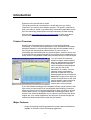
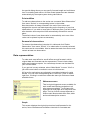
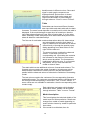
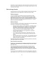
Aura
AutoRelation Analysis?
The expert system in multivariate
adaptive forecasting.
Version 3.1
User Manual
Copyright© 1999 – 2001
Boris Zinchenko & Econom-Expert Ltd.
Moscow – January 2002
The information contained in this guide is subject to change without notice.
Econom-Expert Ltd. shall not be liable for errors contained herein, or for
consequential damages in connection with the furnishing, performance, or use of the
material.
No part of this document may be reproduced or transmitted in any form or by any
means, electronic or mechanical, for any purpose, or translated to another language
without the prior written consent of Econom-Expert Ltd. All products or brand names
used in this guide are trademarks or registered trademarks of their respective
companies.
Econom-Expert Ltd.
Teply Stan 8 - 41
Moscow 117133, Russia
+7 (095) 339-28-58
[email protected]
http://www.geocities.com/aforecasts
Copyright© 1999-2001 Boris Zinchenko & Econom-Expert Ltd.
All Rights Reserved.
2
Contents
INTRODUCTION............................................................................................................................ 4
PRODUCT OVERVIEW ...................................................................................................................... 4
MAJOR FEATURES ........................................................................................................................... 4
STATISTICAL MODELING .......................................................................................................... 6
PROBLEM DESCRIPTION ................................................................................................................... 6
APPLICATION CONCEPT ................................................................................................................... 6
DATA DIMENSIONS .......................................................................................................................... 7
ALGORITHMS .................................................................................................................................. 7
USING AURA .................................................................................................................................. 9
SIMPLE DEFINITIONS ....................................................................................................................... 9
Statistical model......................................................................................................................... 9
Input of model............................................................................................................................ 9
Output of model ......................................................................................................................... 9
Forecasting algorithm................................................................................................................ 9
MASTER MODEL .............................................................................................................................. 9
Model tree ................................................................................................................................. 9
Creation of new model ............................................................................................................. 10
Saving model ........................................................................................................................... 10
Opening model......................................................................................................................... 10
Closing model.......................................................................................................................... 10
Calculation of forecasts............................................................................................................ 11
Inserting new series ................................................................................................................. 11
Deleting series ......................................................................................................................... 11
TIME SERIES ................................................................................................................................. 11
Series name.............................................................................................................................. 11
Model parameters .................................................................................................................... 11
Point addition .......................................................................................................................... 12
Removal of observations .......................................................................................................... 12
DATA REPRESENTATION ................................................................................................................ 12
Welcome screen ....................................................................................................................... 12
Graph ...................................................................................................................................... 12
Table ....................................................................................................................................... 13
Model description .................................................................................................................... 13
DATA EXCHANGE FORMATS ........................................................................................................... 14
Clipboard support.................................................................................................................... 14
Clipboard import ..................................................................................................................... 14
Open financial connectivity ...................................................................................................... 14
FORECASTING MODEL SPECIFICATION .............................................................................. 16
UNIFIED SPECIFICATION OF INTERFACES TO THE EXPERT SHELL AND ALGORITHM LIBRARY .............. 17
Globally identify algorithm in algorithm library ....................................................................... 17
Forecasting core functions ....................................................................................................... 17
Functions to estimate buffers needed ........................................................................................ 20
Functions to tell algorithm capabilities to the framework.......................................................... 21
3
Introduction
Welcome to the Aura® User's Guide.
This guide provides an introduction to Aura® and gives you all the
information you need to work with the product. The guide is intended to
help new users of Aura®. It provides basic information applicable across
the core technology and explains concepts necessary to start working.
Visit our site http://www.geocities.com/aforecasts to learn more about
Aura® and to download the latest demo version of this package.
Product Overview
Aura® Is the automated expert system for multivariate statistical
forecasting. It combines the unique power of full automated multivariate
statistical analysis in unlimited dimensions with the remarkable ease of
use. Be you the experienced mathematician or just a novice in
forecasting with immediate and very practical goals, Aura® is just for you.
It can both offer the instant forecast by one mouse click or expand for you
many levels of complicated model trees that stay behind a few final digits.
You can watch accurate and
attractive charts, detailed tables
and very sophisticated multilevel
model descriptions linked with
intuitive hypertext links designed
not to get you lost in this
abundance of models. You can
instantly import tremendous
amounts of data both from the
desktop applications and external
databases, analyze them with one
mouse click and store to disk with
unique speed in native format as
well as export results for the
further use in many formats.
If you are software developer not interested in these visual features, then
even more you can benefit from Aura® power and flexibility, because it
offers you many levels of simple and effective open user APIs to access
custom data sources, incorporate additional forecasting models, store
results in the external databases of your choice or just embed the whole
engine into your custom application and enjoy all its power through the
customized web interface which best fits your needs.
Major Features
•
Unique forecasting technology based on fractal metanet architecture
capable to combine various forecasting algorithms.
4
•
Multivariate statistical models of arbitrary dimensions in infinite level
layering network.
•
Intuitive user interface with multiscale tables and charts featuring
confidence estimates and residuals.
•
Transparent model structure with multilevel hypertext navigation
delivered through built-in web server.
•
Own standard of superfast unlimited object storage with multi-user
support.
•
Unattended automated operation with the profiling logs and smart
error recovery.
•
Open financial connectivity to all major data vendors through open
standard data drivers.
•
Unlimited extensibility through unified language neutral model
component standard.
5
Statistical Modeling
This chapter discusses the different statistical modeling concepts of and
shows how they are supported by Aura®.
Aura® is a dedicated modeling toolkit for building multivariate statistical
models of very big dimensions and apply them to the live streams of the
real-time data for fast prediction and fast decision making.
Aura® is not just another forecasting algorithm. It implements
computational matanet. The individual knots of this network may be any
forecasting algorithm. Moreover, each knot may hold the whole selfsimilar
network however elaborate and complex.
In this way our project suggests the unique way to integrate all the
imaginable forecasting algorithms into the unified self-organized AI
environment which automatically selects the best combination of
algorithms in each particular case.
Problem description
While there are many computer programs aimed to resolve this problem,
they often fail to meet expectations of a novice user at least in the
following ways:
•
Tightly specialized applications can effectively forecast only a
narrow set of typical situations. The nuisance is, situations tend to
change swiftly.
•
Diverse statistical analyzers require at least a moderate
knowledge of the algorithms they expose. Such knowledge costs
time and money.
•
Powerful and flexible neuronets appear quite dumb on a short data
series. In fact, additional data happen to be expensive, if available
at all.
To consolidate and mutually reinforce the above approaches we suggest
the universal shell built up as an expert system and aimed to combine the
most popular forecasting algorithms in the automated competitive
environment.
Given a multidimensional time series, the system automatically
hypothesizes on a set of all available solutions seeking to minimize the
aggregate difference between backforecasts and the actual values of the
supplied series. The most effective hypotheses then integrate into the
final model which, in turn, is used to predict future responses.
Application concept
Aura® implements the fractal computational network based on the
stochastic propagators. The individual knots of this network may be any
forecasting algorithms.
6
The adjective fractal does not mean that uses Aura® fractal algorithms
for forecasting purposes (although it is fairly possible). It points in current
context that Aura® itself is fractal. In fact, fractal is defined as the
selfsimilar structure produced by a set of invariant derivation rules.
Aura® network is exactly such structure. It can hold infinite number of
modeling levels. Each modeling level can hold the arbitrary amount of
forecasting models. Each model, in turn, obeys the derivation rules of the
homomorphic hierarchy of interfaces and can hold itself infinite layers of
such interfaces in itself. Aura® as such derives exactly from such
interface, so it can hold itself in recursion to infinite order.
Individual forecasting models with the unified interfaces may be
interpreted as the knots of the Aura® fractal network. To connect them
into the optimal forecasting strategy Aura® uses the concept of stochastic
propagators. Each propagator represents the series of stochastic points
with the certain variance estimated for each point. The network uses a
number of optimization techniques to ensure the serial convergence of
propagators to the minimum level of variance. In this way the optimal
forecast is achieved.
In contrast to the most other statistical packages, Aura® operates not on
traditional time series. It operates on individual observation points. So it
can combine in a single model the data with very different time steps,
from fraction of seconds to many years. The user should be very carefully
with input observation dates for each series. They must exactly coincide,
or, else, algorithm will synchronize them on its own.
Data dimensions
With its breakthrough data analysis technology Aura® is able to deal
effectively with data sets of practically any length and dimensions. The
exact characteristics are listed in the following table:
Parameter
Minimum
Maximum
Number of input data series (input dimension
of the model).
1
not restricted
The length of the individual data series.
Different data series within the model may
have different lengths. (We recommend at
least 10 points in a series)
2
not restricted
The length of forecast (we recommend the
values not exceeding 5)
1
not restricted
Algorithms
The set of algorithms currently implemented and available in the package
are listed below. Moreover, each knot may hold the whole selfsimilar
fractal network however elaborate and complex.
At present, the project supports the following:
7
•
Input control procedures for automatic conversion of raw data into
a data series.
•
Monitoring and smart filtering of extreme values within data series.
•
Mutual synchronization and aggregation of datasets.
•
Multidimensional analysis of distributed lags.
•
Simple linear regression (for instant prediction of a very short time
series).
•
A number of statistical tests, which detect seasonal components
and estimate their characteristic times.
•
Non-seasonal ARIMA models for individual forecasting of medium
and long time series.
•
Adaptive selection of seasonal ARIMA models.
•
Multiple linear regression analysis with confidence intervals for the
future responses.
•
Selection of the regression model using a forward stepwise
algorithm.
•
Leaps and bounds algorithm for determining a number of best
regression subsets from a full regression model.
•
Special set of multivariate tests, which assist combining the above
methods into a most effective model.
While most of the above algorithms are widely known and available, the
real power of our solution proceeds from the ability to automatically
merge these computational methods into a flexible and effective forecast
model.
8
Using Aura
Simple definitions
Statistical model
The primary goal of Aura® is adaptive forecasting of the time series. The
forecast is based on statistical model of the series. Statistical model is the
main structural unit of Aura®. Each model consists of input, output and
forecasting algorithm.
Input of model
Input of model consists of arbitrary number of conditionally grouped
observations of any nature and frequency.
Output of model
Output of the model contains the series of forecasts calculated for each
input of the model. Each output represents the time series derived from
input by means of forecasting algorithm.
Forecasting algorithm
Is the function that transforms the input values into forecast. The system
automatically chooses the algorithm that provides the best forecast.
Master model
Master model is the main model which holds any other models
corresponding to current working session. Master model has its name
which expresses its user friendly meaning.
You can change this name any time through
command “Name”from menu “Model”.
Each model can be saved to the separate
permanent storage and reloaded from it later.
Big models can be loaded in parts by
demand saving computer memory and
allowing to work with huge models.
You can explore master model structure in
several ways. The easiest of them is using
model tree.
Model tree
The structure of the model is shown in a special window which usually
resides on the left side of application screen and has the caption
9
“Structure of model”. This window reveals the
whole model structure in a multilevel tree and
guides you through all model components. If
you accidentally closed that window, you can
display it by command “Model Tree”from
menu “View”.
The model tree has the context menu to
expand and collapse its items and get access
to model nodes. Alternatively you can double
click on each node to get access to the
corresponding model.
Creation of new model
To create new master model use command
“New”from menu “File”. Newly created model
contains no time series. To add some series
use data import options from the same menu
or click “Add Series”in menu “Model”.
In the later case the system generates for you
very short sample series which consists of two points. You can use that
series in further work by changing its name and adding additional points
as needed or removing initially created points.
Creating the new master model you automatically close the current active
model.
Saving model
You can save current master model for the later use in a special format of
Aura®. This format actually represents the complex high performance
object storage which permanently holds your full current working state
and the reloads it by demand. The model is saved to the special file with
the extension “*.arm”(AuRaModel). To save model use command “Save”
from menu “File”.
Opening model
All files of Aura® are saved in special files with the extension “*.arm”
(AuRaModel). To open such file from Windows Explorer just double click
on its icon.
To do the same form Aura® shell use command “Open”from menu “File”
or alternatively use the list of recently opened models downside of the
same menu.
Closing model
To close current master model use command “Close”from menu “File”.
Closing the model removes all its views from the screen including
“Structure of model”window.
10
Calculation of forecasts
To calculate forecast just click “Calculate”in menu “Model”. Then the
system automatically searches for the best model and calculates
forecasts using that model. After the calculations are finished all charts
and tables are properly updated.
Calculation of whole model may be very time consuming process. If you
have already done it and then did minor changes to input data, as, say,
added a couple of points to lengthy time series, you don’t have to
recalculate the whole model. You can use command “Update”in the
same menu to just update forecasts using the same model. It’s much
faster and don’t affect the accuracy.
Inserting new series
To insert new series into the model use command “New Series”from
menu “Model”. Simple series with two points is then inserted. New series
are automatically enumerated consequently as “Series 1, 2, … ”you can
change series name and fill it with your data.
Deleting series
To delete the current series from the model use command “Delete
Series”from menu “Model”. This command deletes the series which is
currently displayed in the active window. If no such window is present
then the series highlighted in the model tree is removed. You will be
warned before deletion. Deleted series cannot be restored.
Time series
Generally time series is the sequence of observations ordered according
to their dates. Aura® does not require that observations be separated
with equal periods of time. In this way the actual observation time
becomes the essential part of the model. It drastically distinguishes
Aura® from other statistical packages where only the order of
observations plays role.
Aura® displays the time series and its model as one entity in the model
tree. So you cannot generally distinguish between them.
Series name
Each series in Aura® must have the unique name. That name unifies all
models that descend from this series in one model cluster which expands
from root nodes in the model tree.
You can change series name any time by simply editing it in table head
or by command “Name”from menu “Series”. In this way you
simultaneously rename all models corresponding to this series.
Model parameters
The overall model parameters for each series can be set individually
through command “Tune”from menu “Model”. This command displays
11
the special dialog where you can specify forecast length and confidence
level in modeling each series. All other model parameters are detected
automatically by the expert system during calculations.
Point addition
To add new observations to the series use command “New Observation”
from menu “Series”or corresponding button in the toolbar.
New observation is always inserted in the end of time series and
assigned the correct next date depending on the frequency of previous
observations. If you wish to insert point in different place, just edit its date
after insertion and new point will be automatically relocated to correct
place.
The default value of new observation is automatically set to zero. New
value can be printed in place as necessary.
Removal of observations
To remove the observation just select it in table and click “Delete
Observation”from menu “Series”. If no observation is currently selected,
this command is not available. Also be aware that each time series must
contain at least one observation.
Data representation
To make work most effective Aura® offers several formats in which
original data and forecasts can be represented. Those include charts,
tables and hypertext reports. You can always choose one that best fits
your current needs.
If you get lost in many windows, select “Main Model”in menu “View”or
just click home button on toolbar to return to initial screen.
All forms for each series are collected in one tabbed window for rapid
access. You can click corresponding tab or use menu “View”to select
right form. Clicking in model tree makes the same job. Below are listed
available forms.
Welcome screen
That is original hypertext screen available for
each model and offering navigation to all
other screens available. To navigate click
hyperlinks on that page as on any other web
page. The list of other screens depends on
exact model. Most models offer chart, table
and model description screens.
Graph
This screen displays the original input series, backforecasts for the
series, future forecasts and confidence intervals for forecasts and
12
backforecasts in different colors. Colors and
signs for each graph component are
displayed below. Series name is shown
above the graph. Both series name and
legend can be hidden to extend display
through submenu “Chart”in menu “Format”.
Table
Data tables can have two different formats:
data input table and static table with the back
forecasts. The exact format depends on model level for which the table is
displayed. If the model belongs to upper level of model tree, then the
input table shows allowing for user input of series data. If, on the other
hand, subsidiary model is displayed, then static table takes place which
takes all data from calculated arrays.
The first row of each table contains observation dates. All observations
are automatically sorted by their dates. If
input is enabled, then the date can be edited
either directly or through the special popup
dialog appearing from down button on the
right of active date cell.
The second column contains the observed
values. To edit them just click on
corresponding cell. Input table also contains
the forecasts on the bottom of this column
which cannot be edited. The forecasts are
highlighted in different color. If no forecasts
are present, the you must calculate the
model to observe them.
The static table has two additional columns: forecast and variance. The
forecast column contains the actual forecasts in its bottom as well as
backforecasts calculated for certain period in the past and shown in
parallel with the observed values to estimate the residuals of forecasting
model.
The last column contains the variances of the corresponding forecasts
and backforecasts. The variances are estimated with the confidence level
set through model setup dialog in command “Tune”of menu “Model”. If
some values are not available for estimation, then the corresponding cells
remain empty.
Each table has row header which displays
observation index. Header can be hidden
through submenu “Table”in menu “Format”.
Model description
This form displays the technical details of the
model used for series prediction. Details can
change from model to model depending on
exact solution chosen by Aura® for particular
time series.
If the model is multivariate, then its
13
description contains hyperlinks to other series which influence the current
series. If the model is multilayered, then this page contains also the to the
contained child models.
Data exchange formats
Aura® offers the rich choice of data exchange formats which allow easy
integration with the other applications, export and import of data.
Clipboard support
You can exchange any information with other applications through
standard windows clipboard. To do that just select any region of data
table and click “Copy”from menu “Edit”. Then go to application where
data must be placed and click “Paste”. All data will be moved. In this way
data can be moved to any desktop application as MS Excel. To export
picture use the same commands.
Clipboard import
The same mechanism can be used to import data from other applications
into Aura®. To do that use the following sequence:
•
Select the region of data in source application. The data must be
arranged in the same order as in Aura®, i.e. in two columns with
first column containing dates in standard OLE format (as MS
Excel). The second row must contain observed values. Also
insertion of only one column is possible (dates or values).
•
Copy the selected data from source application to clipboard
through “Copy”command.
•
Go to Aura® and select target series. Open table form of that
series. Select the region in the table where the data should be
placed.
•
Use command “Paste”from menu “Edit”. If the destination series is
shorter than the data in clipboard then the additional rows will be
added to the table as necessary.
The observation will be automatically sorted during insertion so that their
final order can differ from the original.
Open financial connectivity
Probably the most powerful of all interfaces Aura® offers in connecting to
financial data. This functionality is accessed through command “Import”
from menu “File”.
This command displays the special dialog which contains the list of
financial data servers installed on your computer. To select the right
server just double click on its icon or select it and push “Next”. Then
program automatically connects to the server and displays all databases
present on it.
You can see the list of databases on the screen that appears. Select the
right database from the list, open and even create additional databases, if
14
corresponding driver supports these operations. When you decided which
database to open just double click on its icon.
The program automatically connects to the selected database and
displays all its data tables in the left pane of a special dialog. Use the
mouse and special buttons in the middle of the dialog to select tables and
move them to the right list. When done click “OK”and the process of data
import will start. The progress dialog will inform you on which data are
currently imported. Cancel button permits stopping that process any time.
Aura® supports rich choice of standard servers which fully conform to
the latest standards of financial data providers.
Moreover, Aura® offers exceptionally simple, fast and reliable open
standard for development of additional drivers so that independent
developers can supply any drivers of their choice.
15
Forecasting model specification
Each forecasting model consists of three main parts: input, output and
forecasting algorithm. Input of the forecasting model is the collection of
time series. Output of the model is the collection of forecasted time series
with probability limits and backforecasts for the model verification.
Forecasting algorithm is any function transforming input to output
hopefully with the good forecasting accuracy.
Input
l
Input
Forecasting
algorithm
Input
n
Output
Forecast
Output
Forecast
Output
Forecast
n
m
where
l – number of inputs;
k – number of outputs;
n – the length of each input series;
m – the length of each forecast.
Each input is the numeric array of length n.
Each output consists of two numeric arrays, say ArrayForecast and
ArrayVariance, of length (n + m) each. ArrayForecast in its first n
positions contains backforecasts at exactly the same time lags as the
observed points of the input time series. This information must be
produced by forecasting algorithm for model verification. If some of the
backforecasts cannot be calculated, then they must be filled with NaN
values. The last m positions of ArrayForecast must contain forecasts of
one to m steps ahead. ArrayVariance must contain the variances of the
forecasts present in the ArrayForecast exactly in the same order or NaN
if the corresponding variance cannot be obtained.
Corresponding input and output data structures can be implemented in
any programming language as well as a few additional functions for
algorithm control and model storage.
The framework registers any dll that conforms to the specification in
unified algorithm repository and selectively uses them in each case to
provide the best forecast.
16
k
The sample of such interface in C is provided below. Functions are split
in groups for easier navigation. Most functions in dll can be missed. In
that case the framework replaces them with default implementations
which do trivial default processing.
Unified specification of interfaces to the expert shell and
algorithm library
Globally identify algorithm in algorithm library
const char* AlgorithmName()
Return user friendly name of algorithm implemented in the dll. If not
implemented, model name returned to user as valid string “Unknown”.
Forecasting core functions
int CalculateForecasts(int iNumInputs, int iInputLen, double*
pInputMatrix, int iNumOutputs, int iForecastLen, double*
pOutputMatrix, double* pVarianceMatrix, double* pDateTime, char*
pSeriesNames, int iBufLen, void* pModelBuffer, int iParamLen,
char* pModelParameters)
Calculate forecasts. If this function is omited, all forecasts are considered
not existing. This function must be implemented for algorithm to give
any reasonable results.
iNumInputs - Input. Number of input series.
iInputLen - Input. The length of each input series.
pInputMatrix - Input. The array of size exactly (iNumInputs * iInputLen)
containing all input series in the following order. First iInputLen elements
contain first series, next iInputLen – second series, and so on till the last
iNumInputs series.
iNumOutputs- Input. Number of output series.
iForecastLen – Input. The desired length of forecast.
pOutputMatrix – Output. Matrix of dimension (iNumOutputs * (iInputLen +
IforecastLen)) to hold forecasts and backforecasts calculated. On
completion it must hold output series in the following order. First
(iInputLen + IforecastLen) elements must contain the first output series
(see the figure), next (iInputLen + IforecastLen) elements – the second,
and so on till the last iNumOutputs series. Each output series in turn,
must hold in (2,… , iInputLen) locations the backforecasts one step ahead
corresponding to exactly the same observed points of input series or NaN
values, if corresponding backforecast cannot be calculated. Locations
(iInputLen + 1,… , iInputLen + iForecastLen) of the output series must
contain calculated forecasts (1,… , iForecastLen) steps ahead.
pVarianceMatrix – Output. Matrix of dimension (iNumOutputs * (iInputLen
+ IforecastLen)) to hold the variances of forecasts and backforecasts
calculated exactly in the same order as pOutputMatrix.
pDateTime – Input/Output. The array of size (iInputLen + iForecastLen)
which on input contains the timestamps of each observation in its first
17
iInputLen locations. On output the array should contain expected
timestamps of the forecsted values in its last iForecastLen locations and
also may contain NaN values for timestamps of input observations to
indicate that corresponding points were missed by algorithm. NaN
timestamps of forecasted values indicate that estimation of future
timestamps is not supported by algorithm.
pSeriesNames – Input/Output. Null terminated string of names of input
time series separated by new line characters (“\n”) exactly in same order
as they appear on pInputMatrix. On output should contain the names of
output series exactly in same order as they appear in pOutputMatrix.
iBufLen – Input. The size of buffer to hold the model info.
pModelBuffer – Output. The buffer to hold the model info, which can be
used by algorithm next time it is invoked for updates. The framework
supports correct storage of this buffer in binary form. And provides it
exact in all consequent calls. Each algorithm is free to store any info in
this buffer and ask to allocate memory for it.
iParamLen - Input. The size of buffer to hold the model parameters.
pModelParameters – Input. The buffer to hold the model parameters
which specify the various conditions on how to calculate forecasts. This
information can be interactively queried from the user through
SettingsForm(… ) function.
int UpdateForecasts(int iNumInputs, int iInputLen, double*
pInputMatrix, int iNumOutputs, int iForecastLen, double*
pOutputMatrix, double* pVarianceMatrix, double* pDateTime, char*
pSeriesNames, int iBufLen, void* pModelBuffer, int iParamLen,
char* pModelParameters)
Update forecasts based on previously calculated and stored model. If not
supplied, no fast update option is not available for the model. In that case
the function CalculateForecasts() is called with the same set of
parameters and the information contained in pOutputIndex and
pModelBuffer is erased.
iNumInputs - Input. Number of input series.
iInputLen - Input. The length of each input series.
pInputMatrix - Input. The array of size exactly (iNumInputs * iInputLen)
containing all input series in the following order. First iInputLen elements
contain first series, next iInputLen – second series, and so on till the last
iNumInputs series.
iNumOutputs- Input. Number of output series.
iForecastLen – Input. The desired length of forecast.
pOutputMatrix – Output. Matrix of dimension (iNumOutputs * (iInputLen +
IforecastLen)) to hold forecasts and backforecasts calculated. On
completion it must hold output series in the following order. First
(iInputLen + IforecastLen) elements must contain the first output series
(see the figure), next (iInputLen + IforecastLen) elements – the second,
and so on till the last iNumOutputs series. Each output series in turn,
must hold in (2,… , iInputLen) locations the backforecasts one step ahead
corresponding to exactly the same observed points of input series or NaN
values, if corresponding backforecast cannot be calculated. Locations
18
(iInputLen + 1,… , iInputLen + iForecastLen) of the output series must
contain calculated forecasts (1,… , iForecastLen) steps ahead.
pVarianceMatrix – Output. Matrix of dimension (iNumOutputs * (iInputLen
+ IforecastLen)) to hold the variances of forecasts and backforecasts
calculated exactly in the same order as pOutputMatrix.
pDateTime – Input/Output. The array of size (iInputLen + iForecastLen)
which on input contains the timestamps of each observation in its first
iInputLen locations. On output the array should contain expected
timestamps of the forecsted values in its last iForecastLen locations and
also may contain NaN values for timestamps of input observations to
indicate that corresponding points were missed by algorithm. NaN
timestamps of forecasted values indicate that estimation of future
timestamps is not supported by algorithm.
pSeriesNames – Input/Output. Null terminated string of names of input
time series separated by new line characters (“\n”) exactly in same order
as they appear on pInputMatrix. On output should contain the names of
output series exactly in same order as they appear in pOutputMatrix.
iBufLen – Input. The size of buffer to hold the model info.
pModelBuffer – Input. The buffer which holds the model info previously
stored during model calculation.
iParamLen - Input. The size of buffer to hold the model parameters.
pModelParameters – Input. The buffer to hold the model parameters
which specify the various conditions on how to calculate forecasts. This
information can be interactively queried from the user through
SettingsForm(… ) function.
int ModelReport(int iReportLen, char* pReportBuffer, int iBufLen,
void* pModelBuffer,
int iParamLen, void* pModelParameters,
int iPathLen, const char* pResPath)
Describe model based on info stored in buffer while it was calculated. If
not supplied, no reporting option is available for the model.
iReportLen – Input. The size of buffer to hold the report.
pReportBuffer – Output. The buffer where the function must store the
report. Html or text formats are expected.
iBufLen – Input. The size of buffer to hold the model info.
pModelBuffer – Input. The buffer which holds the model info previously
stored during model calculation.
iParamLen - Input. The size of buffer to hold the model parameters.
pModelParameters – Input. The model settings parameters.
iPathLen - Input. The size of buffer to hold the resource path.
pResPath – Input. The url path to the web server which processes the
current model. Developers can upload their own graphics etc. to store on
the server and use in their custom reporting.
int SettingsForm(int iFormLen, char* pFormBuffer, int iBufLen, void*
pModelBuffer, int iParamLen, void* pModelParameters, int iPathLen,
const char* pResPath, const char* pServerName)
19
Prepares the custom web form to ask user for model settings. Returns
the acquired info in the pModelParameters buffer for later use by
CalculateForecasts(… ) and UpdateForecasts(… ) functions. If not
supplied, settings changes are not supported for the model.
iFormLen – Input. The size of buffer to hold the form.
pFormBuffer – Output. The buffer where the function must store the form.
Html format is expected.
iBufLen – Input. The size of buffer to hold the model info.
pModelBuffer – Input. The buffer which holds the model info previously
stored during model calculation.
iParamLen - Input. The size of buffer to hold the model parameters.
pModelParameters – Input. The model settings parameters.
iPathLen - Input. The size of buffer to hold the resource path.
pResPath – Input. The url path to the web server which processes the
current model. Developers can upload their own graphics etc. to store on
the server and use in their custom reporting.
pServerPath – Input. The url path to the web server which will processes
the form.
Functions to estimate buffers needed
int MaxBufferLen(int iNumInputs, int iInputLen, int iNumOutputs, int
iForecastLen)
Returns the buffer allocation size requested from algorithm to hold its
model info. If not implemented, the standard 64 kb is allocated by default.
iNumInputs - Input. Number of input series.
iInputLen - Input. The length of each input series.
iNumOutputs- Input. Number of output series.
iForecastLen – Input. The desired length of forecast.
int MaxParamLen(int iNumInputs, int iInputLen, int iNumOutputs, int
iForecastLen)
Returns the buffer allocation size requested from algorithm to hold its
parameters. If not implemented, the standard 64 kb is allocated by
default.
iNumInputs - Input. Number of input series.
iInputLen - Input. The length of each input series.
iNumOutputs- Input. Number of output series.
iForecastLen – Input. The desired length of forecast.
int MaxReportLen(int iNumInputs, int iInputLen, int iNumOutputs, int
iForecastLen)
Returns the buffer allocation size requested from algorithm to hold its
report. If not implemented, the standard 64 kb is allocated by default.
iNumInputs - Input. Number of input series.
20
iInputLen - Input. The length of each input series.
iNumOutputs- Input. Number of output series.
iForecastLen – Input. The desired length of forecast.
int MaxSettingsLen(int iNumInputs, int iInputLen, int iNumOutputs,
int iForecastLen)
Returns the buffer allocation size requested from algorithm to hold its
model settings web form. If not implemented, the standard 64 kb is
allocated by default.
iNumInputs - Input. Number of input series.
iInputLen - Input. The length of each input series.
iNumOutputs- Input. Number of output series.
iForecastLen – Input. The desired length of forecast.
Functions to tell algorithm capabilities to the framework
int MinInputLen()
Returns the minimum length of input. Default is 1.
int MaxInputLen()
Returns the maximum length of input. Default is MAX_INT.
int MinForecastLen()
Returns the minimum forecast length. Default is 1.
int MaxForecastLen()
Returns the maximum forecast length. Default is MAX_INT.
int MinNumInputs()
Returns the minimum number of inputs. Default is 1.
int MaxNumInputs()
Returns the maximum number of inputs. Default is MAX_INT.
int MinNumOutputs()
Returns the minimum number of outputs. Default is 1.
int MaxNumOutputs()
Returns the maximum number of outputs. Default is MAX_INT.
Of all listed functions only one must be implemented to ensure the full
functionality of the algorithm within the framework. Namely,
CalculateForecasts(… ) all other functions can be safely omitted from
implementation, if their default functionality is sufficient and complies to
the particular algorithm.
Implemented functions from the above list must be compiled into
standard windows DLL and exported from it properly. It can be done in
any programming language. The resulting DLL module must then be
placed into the /ModelDrv subfolder of the original application folder tree.
21
The application must be restarted in order to recognise the newly
supplied algorithm.
22