Download Molecular Dynamics Simulation Program MARBLE User`s Manual

Molecular Dynamics Simulation Program
MARBLE
User's Manual
ver. 0.6.0.1
About this manual
This document is the manual for "MARBLE", a molecular dynamics simulation program. This manual is
still a beta version and principally composed of tutorials. Various calculation examples and commands for
MARBLE, as well as the "molx" pre-processing program, will be added to this manual in the future. Please feel
free to contact us if you have any feedback or find any flaws or defects in the manual descriptions.
September 29, 2012
MARBLE Manual Editorial Committee
Table of Contents
1.
Introduction ....................................................................................................................................................... 2
1.1. What is MARBLE? ..................................................................................................................................... 2
1.2. License......................................................................................................................................................... 2
1.3. Citation ........................................................................................................................................................ 2
2.
Installation ......................................................................................................................................................... 3
3.
Tutorials ............................................................................................................................................................ 5
3.1. Calculation flow .......................................................................................................................................... 5
3.1.1.
Executing the molx ............................................................................................................................ 5
3.1.2.
Files generated in the molx ................................................................................................................ 5
3.1.3.
Executing MARBLE.......................................................................................................................... 6
3.1.4.
Files generated in MARBLE ............................................................................................................. 6
3.1.5.
Parallel computation in MARBLE..................................................................................................... 7
3.2. Constructing the system with the molx ....................................................................................................... 8
3.2.1.
Before executing the molx ................................................................................................................. 8
3.2.2.
Example of the molx calculation – 1: Lysozyme ............................................................................ 9
3.2.2.1.
Before executing the molx ......................................................................................................... 9
3.2.2.2.
Executing the molx .................................................................................................................. 10
3.2.3.
Example of the molx calculation – 2: F1 motor............................................................................ 14
3.2.3.1.
Before executing the molx ....................................................................................................... 14
3.2.3.2.
Executing the molx .................................................................................................................. 15
3.3. MARBLE .................................................................................................................................................. 21
3.3.1.
Energy minimization (with example of lysozyme) .......................................................................... 21
3.3.2.
Molecular dynamics calculation ...................................................................................................... 23
3.3.2.1.
Molecular dynamics simulation of lysozyme aqueous solution system .................................. 23
3.3.2.1.1. Equilibration (increasing the temperature to that for simulation) ......................................... 23
3.3.2.1.2. Equilibration (removing restraints gradually) ....................................................................... 25
3.3.2.1.3. Production run (NVT ensemble) ........................................................................................... 26
3.3.2.1.4. Production run (NPT ensemble) ........................................................................................... 27
3.3.2.2.
Targeted MD of the transition from closed to open conformation of F1 motor ....................... 28
4.
Execution Procedure for the molx and MARBLE (for K computer and FX10).............................................. 32
4.1. Execution procedure for the molx ............................................................................................................. 32
4.2. Execution procedure for MARBLE ........................................................................................................... 32
4.2.1.
Using d_grid .................................................................................................................................... 33
4.2.2.
Specifying the data directly ............................................................................................................. 33
5.
Command Reference ....................................................................................................................................... 35
5.1. The molx.................................................................................................................................................... 35
5.1.1.
Force field ........................................................................................................................................ 35
5.1.2.
Input ................................................................................................................................................. 35
5.1.3.
Output .............................................................................................................................................. 35
5.1.4.
Model building................................................................................................................................. 36
5.1.5.
System building ............................................................................................................................... 37
5.2. MARBLE .................................................................................................................................................. 38
5.2.1.
[input] .............................................................................................................................................. 39
5.2.2.
[output] ............................................................................................................................................ 39
5.2.3.
[init] ................................................................................................................................................. 39
5.2.4.
[restraint].......................................................................................................................................... 40
5.2.4.1.
position_harmonic ................................................................................................................... 40
5.2.4.2.
rmsd ......................................................................................................................................... 41
5.2.5.
5.2.6.
5.2.7.
5.2.8.
5.2.9.
5.2.10.
[constraint] ....................................................................................................................................... 41
[PT_control] ..................................................................................................................................... 42
[nonbond]......................................................................................................................................... 42
[ewald] ............................................................................................................................................. 43
[min] ................................................................................................................................................ 44
[md] ................................................................................................................................................. 44
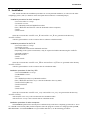
1.Introduction
1. Introduction
1.1. What is MARBLE?
MARBLE (MoleculAR simulation program for BiomoLEcules) is a molecular simulation program
developed to carry out simulations of various biopolymers including proteins.
The features of MARBLE are as follows:
 It employs a symplectic rigid-body time integration scheme, achieving total energy conservation with
high precision.
 It implements the PME (Particle Mesh Ewald), a standard algorism for calculating long-range
interactions.
 It is compatible with the OpenMP multiprocessing framework, where the computation is parallelized
based on divisions of the simulation system space.
1.2. License
The license of MARBLE conforms to the GPL (GNU General Public License).
1.3. Citation
When publishing research results using MARBLE, please cite the following article:
Ikeguchi M (2004) Partial rigid-body dynamics in NPT, NPAT and NPγT ensembles for proteins and
membranes. J Comput Chem 25(4): 529-541.
2
2.Installation
2. Installation
This section describes the installation procedure for several particular machines, as well as for the other
computing systems. (The "$" character in the description below indicates a command prompt.)
Installation procedure for the K computer
$ tar xvfz marble-x.x.x.tar.gz
$ cd marble-x.x.x/src
$ ln –s Makefile.machine.K Makefile.machine
(Here, "Makefile.machine.K" is the file dedicated to the K computer.)
$ make
$ make install
Then, the execution files "marble.x.x.x_K" and "molx.x.x.x_K" are generated in the directory
"marble-x.x/bin/".
*All files generated here are the execution files to submit to calculation nodes.
Installation procedure for the FX10
$ tar xvfz marble-x.x.x.tar.gz
$ cd marble-x.x.x/src
$ ln –s Makefile.machine.FX10 Makefile.machine
(Depending on the system environment, it may be required to load the FFTW using the "module"
command as follows.)
$module load fftw
$ make
$ make install
Then, the execution files "marble.x.x.x_FX10" and "molx.x.x.x_FX10" are generated in the directory
"marble-x.x/bin/".
*All files generated here are the execution files for calculation nodes.
Installation procedure for the Cray XE6
$ tar xvfz MARBLE-x.x.x.tar.gz
$ cd MARBLE-x.x.x/src
$ cd src
$ ln -s Makefile.machine.cray Makefile.machine
(Here, "Makefile.machine.cray" is the file dedicated to the Cray XE6.)
$ module load PrgEnv-cray
$ module load fftw
$ make
$ make install
Then, the execution files "marble.x.x.x_cray" and "molx.x.x.x_cray" are generated in the directory
"marble-x.x/bin/".
*The marble.x.x.x-cray is the execution file for calculation nodes
*The molx.x.x.x-cray is the execution file for calculation nodes
Installation procedure for other computers
The MARBLE operation has currently been confirmed only on the three computing systems above. Even
so, it should work on many other parallel computers since the program is written in C language with OpenMP,
MPI and FFTW3. To install MARBLE to a system other than above, use the following procedure:
3
2.Installation
(1) Installing the FFTW3
Check whether or not the FFTW3 exists in the system where MARBLE is installed. If it does, check
the compilation procedure by referring to the FFTW3 manuals, and proceed to the next procedure "(2)
Modifying the Makefile.machine file". If not, download the FFTW 3.x from the following link and
install it to your environment:
http: //www.fftw.org/
(2) Modifying the Makefile.machine file
Copy the "Makefile.machine.x (x=intel, gnu)" located in the directory "marble-x.x.x/src"
changing the filename to "Makefile.machine". Then modify the file in accordance with the
installation environment. The content of "Makefile.machine" is as follows:
> more Makefile.machine
#
# Makefile Setting for icc + openmpi
#
# for parallel programs
PCC
= mpicc
# C compiler for MPI programs
PCOPTFLAG
= -std=gnu99 -O3 -D_FILE_OFFSET_BITS=64 -D_LARGEFILE_SOURCE
PCOMPFLAG
= -openmp -D_OPENMP
# OpenMP option
PLD
= mpicc
# Linker for MPI programs
PLIBFLAG
=
# Flag of linked libraries (e.g., -lm)
PARCH
= -intel
# Suffix of the system to be compiled
CC
= icc
# C compiler for serial programs
COPTFLAG
= $(PCOPTFLAG)
# Optimization option for serial programs
LD
= icc
# Linker for serial programs
LDFLAG
=
# Linker flag for serial programs
LIBFLAG
=
# Flag of linked libraries (e.g., -lm)
LIBDIR
=
# Flag of directory of linked library
ARCH
= $(PARCH)
# Suffix of the system to be compiled
MARBLEHOME
= ../..
BINDIR
= $(MARBLEHOME)/bin
# Installation directory of execution file
DATDIR
= $(MARBLEHOME)/data
# Installation directory of data file
FFTW_DIR
= /home/xxx/pub/fftw-3.3.2-install
# Installation destination of FFTW
FFTW_INCLUDE
= $(FFTW_DIR)/include
# FFTW header directory
FFTW_LIBDIR
= $(FFTW_DIR)/lib
# FFTW library directory
FFTW_LIB
= $(FFTW_LIBDIR)/libfftw3.a
# FFTW library
#Optimization option
# for serial programs
# for FFTW
(3) Executing "make" and "make install"
4
3.Tutorials
3. Tutorials
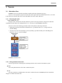
3.1. Calculation flow
MARBLE carries out molecular simulations with the following calculation processes.
The user is first required to prepare structural data of the target molecule in PDB format files (i.e. the files
in the format for structural data in the Protein Data Bank, hereafter called "pdb files").
3.1.1. Executing the molx
Usage: molx input_file
Using the molx, construct the desired simulation system for the target molecule, and generate data files
containing structural data, force field parameters, etc., necessary for the MARBLE calculation.
The molx executes the following procedure based on the pdb file of the target molecule:
 Adds hydrogen atoms and chemical modifications (e.g. disulfide bonds, etc.), on target molecule
(model building)
 Constructs the molecular simulation system by defining a periodic boundary box and adding water
molecules, ions, etc. (system building)
MARBLE calculation flow
3.1.2. Files generated in the molx
The molx generates the following files containing the data of the constructed simulation system.
pdb file
This is the pdb format file of the entire constructed system.
crd file
This file contains the coordinate data of the entire constructed system. MARBLE performs calculations
using the coordinate data in this file.
5
3.Tutorials
mdat file
This file contains the force field parameters for the constructed system used to carry out molecular
dynamics simulations.
3.1.3. Executing MARBLE
Usage: marble input_file output_file
Using the crd and mdat files generated in the molx, perform molecular simulations with MARBLE.
MARBLE performs calculation by the following three steps:
(1) Energy minimization
(2) Equilibration
(3) Production run
These calculations are performed based on crd files obtained from the previous calculation, as well as
mdat files generated in the molx.
3.1.4. Files generated in MARBLE
MARBLE generates the following files:
pdb file
This file contains the coordinate data of the final structure of the simulation system during MARBLE
execution.
crd file
This file contains the final data sets of the simulation system. (Note that during molecular dynamics
simulations, the output also includes the final coordinates, velocity, simulation ensemble, periodic boundary box
data and temperature/pressure control parameters.) The user can restart the molecular dynamics simulation with
the same condition by using this file.
trj file
During molecular dynamics simulations, the system time course data (coordinate sets, velocity sets and
periodic boundary box data) are written to trj files. The user can specify the data content to save in trj files, as
well as the time intervals to save these data, using input files.
out file
This file contains user readable information of molecular simulation such as energy, pressure, temperature,
calculation speed, etc. The user can specify the time intervals to save these data, using input files.
prop file
Outputs various change amounts during calculation. (Some of the information is the same as that of out
files.)
6
3.Tutorials
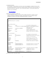
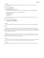
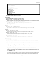
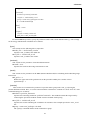
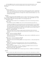
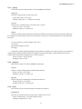
3.1.5. Parallel computation in MARBLE
MARBLE has been developed to perform hybrid parallelization with MPI and OpenMP. MARBLE
performs simulating calculations while parallelizing the processes as shown in the figure below:
Cell divisions and process arrangement in MARBLE
 Dividing the simulation system space into multiple cells at even intervals in X, Y, and Z directions (i.e.
the cubes indicated with dotted lines in Figure (1)).
 Arranging the processes for parallel computation in X, Y, and Z directions (i.e. the cubes enclosed with
red lines in Figure (2)).
 Dividing each of the arranged processes so that the fragmented process takes charge in the calculation
of multiple neighboring cells located in the space where the process is arranged.
In order to speed up simulations, MARBLE parallelizes computing processes as above, and permits data
communications only between neighboring cells.
For this reason, performing MARBLE calculation requires the following data:
(a) The number of cell divisions in the system in X, Y, and Z directions
(b) The number of processes used
(c) The number of processes arranged in X, Y, and Z directions
The data (a) determines the state in Figure (1), and the data (b) and (c) determine that in Figure (2).
Furthermore, on top of (a) to (c) above, the following item is also required:
(d) The number of grids made by dividing the space at even intervals in X, Y, and Z directions to calculate
electrostatic interactions with PME (Particle Mesh Ewald) method
The items (a) to (d) must be determined so that they satisfy their specific rules.
To specify these data parameters for MARBLE calculations, there are the following two methods:
(1) Setting up the d_grid
In this method, once the user specifies the data (b) (the number of processes), and the grid interval
(d_grid) used for PME grid definition, the program automatically determines the data (a), (c), and (d),
and performs calculation.
With this method, the user can easily determine the data (a) to (d). However, when the system box
size is changed as in NPT ensembles, the numbers of grids and cell divisions for PME may also
change. In this case, energy may not be conserved properly, particularly when performing molecular
simulations continuously with different input files.
(2) Directly entering the data (a) to (d) in input files
As described above, although the user can easily determine the data (a) to (d) by using d_grid, the
number of grids for PME method (data (d)) may change depending on the box size. The method
7
3.Tutorials
above is thus unsuitable for box-size variable simulations (such as in NPT ensemble), where the
number of grids for PME method, as well as the PME accuracy, may change at a restart of
simulations.
To avoid these difficulties, the user can directly enter the data (a) to (d) in input files.
See the chapter 4 for the actual settings and examples of executing the above parallel computation.
Note that the procedure for specifying the number of processes and submitting jobs during MPI
parallel computation vary depending on the computing system. For those procedures, refer to the
user's manual for each computing system.
3.2. Constructing the system with the molx
3.2.1. Before executing the molx
MARBLE is designed to carry out molecular simulations with the CHARMM force field. Before using
MARBLE, download necessary CHARMM force fields from the following website:
http: //mackerell.umaryland.edu/CHARMM_ff_params.html
The molx requires the system coordinates in order to generate two files (mdat and crd files) necessary for
MARBLE execution. It is ideal in that the user can prepare the coordinate data of water molecules, ions, all
atoms in protein molecules with hydrogen, and periodic boundary box data. If the user has created a pdb file
containing all these data with an external program, the molx can generate the mdat and crd files immediately.
However, it is rare that the user can prepare the complete structure of target protein molecules with
hydrogen, let alone the data of aqueous solution of the simulation system. Furthermore, the actual target protein
may involve unique chemical bonds, such as disulfide bonds, in its structure. In this case, it is necessary to
complement the data to the simulation system.
For this reason, the molx implements the modeling functions (model building and system building) to
complement the missing data to the simulation system.
The modeling functions available in the molx are as follows:
(1) Complementing atoms missing in the protein conformation (model building)
The molx complements all missing hydrogen and side chain atoms according to the structure template
of each amino acid available in the CHARMM force field.
(2) Defining chemical modifications such as disulfide bonds (model building)
Some proteins may involve chemical modifications where amino acids bind to various molecules or
bind each other as in disulfide bonds. The molx can reproduce these chemical modifications using the
"patch" command.
(3) Generating water molecules and ions around the protein to construct aqueous solution system (system
building)
The molx defines a periodic boundary box, places the protein in the center, and then places water
molecules and ions to generate a protein-aqueous solution system.
8
3.Tutorials
Before executing the molx, be sure therefore to check the target protein conformation regarding the
following items:
(a) Any missing atoms in the protein
Check if there is any missing heavy atom other than hydrogen. If there is any domain involving
the main chain where no atomic coordinate data exist, the molx may not be able to complement
the missing atoms properly. In this case, complement the missing data with an external modeling
program, such as "modeller", before the molx execution.
(b) Any multiconformer
Some data of protein crystal structure may contain multiple side chain conformations as
multiconformer. In this case, since the molx cannot determine which side chain data to be used
for computation, the user is required to decide which conformation to use and edit the pdb file
accordingly.
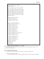
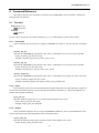
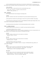
(c) Determining protonation state of amino acid
Charged amino acids and polar amino acids (such as aspartic acid, glutamic acid, lysine, arginine,
and histidine) have multiple protonation states on side chains and the states keep changing due to
the local environment. In this case, the user is required to determine which protonation state to
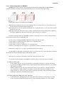
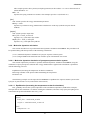
employ for the relevant amino acid side chain before actual computation. Note in particular that
histidine has two states where the side chain charge is neutral, and the states vary depending on
the formulation of hydrogen bonds with surrounding atoms (see the figure below).
Examples of protonation states of histidines
(d) Any disulfide bond
The molx cannot determine if there is any disulfide bond only from the coordinate data in pdb
files. The user is required to check it by referring to the SSBOND data in pdb files, etc.
3.2.2. Example of the molx calculation – 1: Lysozyme
This section describes an example of executing the molx on the lysozyme crystal structure (PDB_ID:
193L).
3.2.2.1. Before executing the molx
First check the items (a) to (d) in the previous section "3.2.1 Before executing the molx".
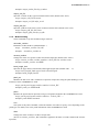
(a) Any missing atoms in the protein
There is no missing heavy atom in 193L.
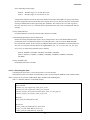
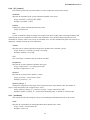
(b) Any multiconformer
In the 193L structure, two conformers exist for each of LYS1, ASN59, SER86, and VAL109. Here, we
select the conformer A for each side chain, and modify the PDB file while referring to the
9
3.Tutorials
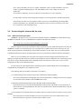
OCCUPANCY value. The following figure describes the example of modifying LYS1.
Modifying multiconformers
(c) Determining protonation state of amino acid
Define all existing charged amino acids to be in a charged state. Now, note that histidine has three
protonation states as mentioned in "Before executing the molx", and two of them, HSD and HSE,
have neutral side chains. Although HIS51 exists in 193L, select HSE here.
(d) Any disulfide bond
The SSBOND description in the PDB file header indicates that the 193L has four disulfide bonds, as
shown below:
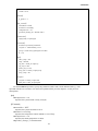
3.2.2.2. Executing the molx
Considering the items above, create an input file to execute the molx. The following shows an example of
constructing a water system using the PDB file of the lysozyme X-ray structure (193L.pdb).
(The ">" character indicates a command prompt.)
> more molx2.in
#Force field#
charmm_top_file ../../toppar/top_all27_prot_na.rtf
charmm_par_file ../../toppar/par_all27_prot_na.prm
#Input#
input_pdb_file ../../pdbfile/193L.pdb
#Output#
output_mdat_file 193L_w.mdat
output_crd_file 193L_w.crd
output_pdb_file 193L_w.pdb
#Model building#
alias CD CD1
alias HOH TIP3
alias O OH2
alias O OT1
rename_residue 15A HSE
patch DISU 6A 127A
patch DISU 30A 115A
patch DISU 64A 80A
patch DISU 76A 94A
10
3.Tutorials
patch_ter NTER 1A
patch_ter CTER 129A
#System building#
solvent_pdb_file watbox216.pdb
solvent_cube on
align_axis diagonal
solvent_buffer 15
ion_placement random
ion SOD CLA
The content of the molx input file is as follows:
# Force field#
The force field for this calculation is specified as follows:
 charm_top_file ../../toppar/top_all27_prot_na.rtf
Specifies the top file of the charmm27 force field for proteins and nucleic acids (top_all27_prot_na.rtf).
 charm_par_file ../../toppar/par_all27_prot_na.prm
Specifies the par file of the charmm27 force field for proteins and nucleic acids
(par_all27_prot_na.prm).
#Input#
 input_pdb_file ../../pdbfile/193L.pdb
Specifies the file containing the structure of the calculation target molecule (193L.pdb).
#Output#
 output_mdat_file 193L_w.mdat
Specifies the name of the mdat file output by executing the molx as "193L_w.mdat".
 output_crd_file 193L_w.crd
Specifies the name of the crd file output by executing the molx as "193L_w.crd".
 output_pdb_file 193L_w.pdb
Specifies the name of the pdb file output by executing the molx as "193L_w.pdb".
#Model building#
The following items are specified:
 The alias command changes the atomic names used in the input PDB file to those in the CHARMM
force field.
 The rename_residue command defines the histidine protonation state by renaming the residue name
of HIS51 to HSE.
 The patch command applies the DISU patch defining disulfide bonds.
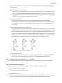
 The patch_ter command applies the NTER and CTER patches defining the N- and C-terminus
structures, respectively.
The "patches" are the scripts to specify chemical modifications (such as disulfide bond and
protonation state) prepared in the CHARMM force field. For the types of patches and their usage, refer
to the CHARMM top files.
In the example above, the residues in "rename_residue", "patch", and "patch_ter" are specified in
the order of residue number and chain ID, as in "patch DISU 6A 127A". Even so, the specification
11
3.Tutorials
can be made in the reverse order, as in "patch DISU A6 A127". Write the chain ID first particularly
when the residue number is a negative value.
#System building#
The box, solvent, and ions for simulations are set up by the following processes:
 solvent_pdb_file watbox216.pdb
Specifies the original structure of water molecules to "watbox216.pdb", where 216 water molecules
are randomly arranged in the cube with a side length of 18.77Å. By arranging water data in this file
periodically, the user can fill water in the periodic boundary box defined in the next step.
 solvent_cube on
Specifies the periodic boundary box as a cube.
 align_axis diagonal
Specifies how to place the protein in the defined periodic boundary box. The molx defines a periodic
boundary box by arranging water with the thickness specified with "solvent_buffer", from the
maximum and minimum coordinates of the protein in X, Y, and Z directions.
The "align_axis diagonal" aligns the longitudinal direction of the protein's principal axis of inertia to
the box diagonal line. (This operation allows decreasing the size of the periodic boundary box).
 solvent buffer 15
Specifies the solvent thickness of 15Å from the protein placed at the center of the periodic boundary
box to each box face.
 ion_placement random
Places ions randomly in the simulation system.
 ion SOD CLA
Specifies chlorine ions (CLA) and sodium ions (SOD) for anions and cations, respectively. Any other
ions in the CHARMM file can also be specified. (Refer to the top file, etc.) Note that only monovalent
ions can be used for anions and cations. Be sure to place ions with the minimum amount necessary to
neutralize the total charge of the system.
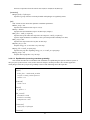
When executing the molx with the input file above, the output is as follows:
> molx.0.5.11b molx.in
****************************************
Molx (Version 0.5.11b)
Host: bits1
Date: Wed Aug 22 12:26:17 2012
Control File: molx.in
****************************************
CHARMM TOP FILE: ../../toppar/top_all27_prot_na.rtf
Version 31.1
Number of types of atomic mass : 158
Number of residues : 37
Number of residues for patching : 31
CHARMM PAR FILE: ../../toppar/par_all27_prot_na.prm
Number of bond types: 257
Number of angle types: 656
Number of dihedral types: 1127
Number of improper dihedral types: 70
Number of cmap dihedral types: 6
12
3.Tutorials
Number of nonbonded atom types: 158
Number of modified nonbonded atom pairs: 0
PDB FILE: ../../pdbfile/193L.pdb
Number of atoms : 1001
Number of hetero atoms : 144
Number of residues : 273
Renaming residue 15A HIS -> HSE
Warning: CMAP term not assigned: -C N CA C N CA C +N in residue 1A
Warning: CMAP term not assigned: -C N CA C N CA C +N in residue 129A
Patching DISU to CYS(6A) and CYS(127A)
Patching DISU to CYS(30A) and CYS(115A)
Patching DISU to CYS(64A) and CYS(80A)
Patching DISU to CYS(76A) and CYS(94A)
Patching NTER to LYS(1A)
Patching CTER to LEU(129A)
1243 atoms are missing in pdb file.
Coordinates of hydrogens of 142 crystal waters are generated.
All Coordinates are determined.
142 waters are found in input pdb file.
1 cations are found in input pdb file.
1 anions are found in input pdb file.
Align principal axes of molecules.
Align the longest axis to diagonal of a cube
Setup of Solvation.
Minimum and maximum coordinates of solute:
(-19.13,-16.18,-22.41)-(19.67,17.41,20.26)
solvent_buffer 15.00 Angstrom
solvent_cube option: on
All atoms are shifted: (36.06,35.72,37.41)
Simulation box is configured as (72.66,72.66,72.66)
Solvent PDB file:
PDB FILE: watbox216.pdb
Number of atoms : 648
Number of hetero atoms : 0
Number of residues : 216
Box Size of Input Solvent PDB: (18.77,18.77,18.77)
Duplicated: (4,4,4)
solvent_radius 1.40 Angstrom
solvent_exclusion_layer 0.00 Angstrom
ION: Grid Spacing (1.00,1.00,1.00)
ION: Number of Grid (73,73,73)
ION: placement random
ION: ion_cutoff 7.40 Angstrom
ION: solvent_radius 1.40 Angstrom
ION: ion_exclusion_layer 4.00 Angstrom
13
3.Tutorials
ION: ion2_exclusion_layer 2.00 Angstrom
ION: Starting to Charge Grid Done
ION: SOD 0, CLA 8
ION: anion CLA (10.09,10.13,9.55) by random
ION: anion CLA (14.35,3.11,6.71) by random
ION: anion CLA (12.82,16.72,43.93) by random
ION: anion CLA (16.77,45.42,33.76) by random
ION: anion CLA (9.53,31.58,28.33) by random
ION: anion CLA (4.50,22.08,30.62) by random
ION: anion CLA (33.41,62.03,52.86) by random
ION: anion CLA (38.16,15.64,8.34) by random
ION: SOD 0, CLA 8
PDB FILE: configured_solvent
Number of atoms : 34878
Number of hetero atoms : 0
Number of residues : 11626
0 atoms are missing in pdb file.
Molecular Data (mdat) Information:
Number of atoms: 37274
Number of atom types: 37
Number of residues: 11907
Number of molecules: 11779
Number of bonds: 37288
Number of bond types: 69
Number of angles: 15315
Number of angle types: 151
Number of dihedrals: 5187 (term: 5391)
Number of dihedral types: 185
Number of impropers: 351
Number of improper types: 14
Number of cmap terms: 127
Number of cmap types: 4
Number of solute molecules: 1
Total charge: -0.000000
Periodic Boundary Box:
72.66 0.00 0.00
0.00 72.66 0.00
0.00 0.00 72.66
3.2.3. Example of the molx calculation – 2: F1 motor
This section describes an example of executing the molx on a dimer (chains B and F) on the F1 motor
crystal structure (PDB_ID: 2JBI).
3.2.3.1. Before executing the molx
First check the items (a) to (d) in the previous section "3.2.1 Before executing the molx".
(a) Any missing atoms in the protein
On the chains B and F for 2JBI calculation, the positional data of all atoms are missing in the domains
14
3.Tutorials
in the following residue ranges:
chain B: Residue ranges 1 to 22 and 402 to 409
chain F: Residue ranges -4 to 9 and 475 to 478
Among these domains, the 402 to 409 on the chain B is located in the middle of a protein. The chain
B will be separated if the structural data of this region does not exist. We here therefore construct the
missing coordinate data of this region using the "modeller". We can leave the rest of the regions as
they are, since they are N- or C-terminus and no functional effect will occur even though the data are
missing.
(b) Any multiconformer
No multiconformer exist in the chains B and F structures on 2JBI.
(c) Determining protonation state of amino acid
Define all existing charged amino acids to be in a charged state. Now, note that histidine has three
protonation states as mentioned in "Before executing the molx", and two of them, HSD and HSE,
have neutral side chains. In the structure of 2JBI, the chain B has five histidines (residue numbers 42,
263, 302, 471, and 476) and the chain F has eight histidines (52, 117, 177, 198, 328, 367, 427, and
451). Here, we define the protonation state as follows:
chain B: 42(HSD), 263(HSD), 302(HSE), 471(HSD), 476(HSD)
chain F: 52(HSE), 117(HSE), 177(HSE), 198(HSD), 328(HSD), 367(HSE), 427(HSD),
451(HSE)
(d) Any disulfide bond
No disulfide bond exists in 2JBI.
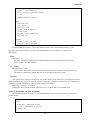
3.2.3.2. Executing the molx
Considering the items above, create an input file to execute the molx.
The following shows an example of constructing a water system using the PDB file of the chains B and F
on the F1 motor X-ray structure (2JBI_BFsub.pdb), modified with modeling data.
(The ">" character indicates a command prompt.)
> cat molx.in
#Force field#
charmm_top_file toppar/top_all27_prot_na.rtf
charmm_par_file toppar/par_all27_prot_na.prm
charmm_toppar_file toppar/stream/toppar_all27_na_nad_ppi.str
charmm_toppar_file toppar_all27_na_po4.str
#Input#
input_pdb_file 2JDI_BFsub.pdb
#Output#
output_mdat_file 2JDI_BFsub_molx.mdat
output_crd_file 2JDI_BFsub_molx.crd
output_pdb_file 2JDI_BFsub_molx.pdb
15
3.Tutorials
#Model building#
alias ANP ATP
alias N3B O3B
alias OXT OT2
alias O OT1
alias CD CD1
alias HOH TIP3
alias WAT TIP3
alias OW OH2
alias O OH2
alias O OT1
alias H1 HT1
alias H2 HT2
alias H3 HT3
alias H HN
alias HG HG1
alias HD11 HD1
alias HD12 HD2
alias HD13 HD3
alias NA SOD
alias CL CLA
rename_residue 42B HSD
rename_residue 263B HSD
rename_residue 263B HSD
rename_residue 302B HSE
rename_residue 471B HSD
rename_residue 476B HSD
rename_residue 52F HSE
rename_residue 117F HSE
rename_residue 177F HSE
rename_residue 198F HSD
rename_residue 328F HSD
rename_residue 367F HSE
rename_residue 427F HSD
rename_residue 451F HSE
patch_ter NTER 23B
patch_ter CTER 510B
patch_ter NTER 9F
patch_ter CTER 474F
#System building#
solvent_pdb_file watbox216.pdb
solvent_buffer 14
align_axis on
ion SOD CLA
16
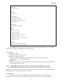
3.Tutorials
The content of the molx input file is as follows:
# Force field#
The force field for this calculation is specified as follows:
 charm_top_file toppar/top_all27_prot_na.rtf
Specifies the top file of the charmm27 force field for proteins and nucleic acids (top_all27_prot_na.rtf).
 charm_par_file toppar/par_all27_prot_na.prm
Specifies the par file of the charmm27 force field for proteins and nucleic acids
(par_all27_prot_na.prm).
 charm_toppar_file toppar/toppar_all27_na_nad_ppi.str
Specifies the toppar file of the charmm27 force field for ATP (toppar_all27_na_nad_ppi.str).
 charm_toppar_file toppar_all27_na_po4.str
Specifies the toppar file of the charmm27 force field for phosphoric acid (toppar_all27_na_po4.str).
#Input#
 input_pdb_file 2JDI_BFsub.pdb
Specifies the file containing the structure of the calculation target molecule (2JDI_BFsub.pdb).
#Output#
 output_mdat_file 2JDI_BFsub_molx.mdat
Specifies the name of the mdat file output by executing the molx as "2JDI_BFsub_molx.mdat".
 output_crd_file 2JDI_BFsub_molx.crd
Specifies the name of the crd file output by executing the molx as "2JDI_BFsub_molx.crd".
 output_pdb_file 2JDI_BFsub_molx.pdb
Specifies the name of the pdb file output by executing the molx as "2JDI_BFsub_molx.pdb".
#Model building#
The following items are specified:
 The alias command changes the atomic names used in the input PDB file to those in the CHARMM
force field.
 The rename_residue command defines the histidine protonation state by renaming the residue name.
 The patch_ter command applies the NTER and CTER patches to the structure definition of the Nand C-terminus on chains B and F, respectively.
In the example above, the residues in "rename_residue", "patch", and "patch_ter" are specified in the
order of residue number and chain ID, as in "patch DISU 6A 127A". Even so, the specification can be made
in the reverse order, as in "patch DISU A6 A127". Write the chain ID first particularly when the residue
number is a negative value.
#System building#
The box, solvent, and ions for simulations are set up by the following processes:
 solvent_pdb_file watbox216.pdb
Specifies the original structure of water molecules to "watbox216.pdb", where 216 water molecules
are randomly arranged in the cube with a side length of 18.77Å. By arranging water data in this file
periodically, the user can fill water in the periodic boundary box defined in the next step.
 solvent_cube on
Specifies the periodic boundary box as a cube.
 align_axis diagonal
17
3.Tutorials
Specifies how to place the protein in the defined periodic boundary box. The molx defines a periodic
boundary box by arranging water with the thickness specified with "solvent_buffer", from the
maximum and minimum coordinates of the protein in X, Y, and Z directions.
The "align_axis diagonal" aligns the longitudinal direction of the protein's principal axis of inertia to
the box diagonal line. (This operation allows decreasing the size of the periodic boundary box).
 solvent buffer 15
Specifies the solvent thickness of 15Å from the protein placed at the center of the periodic boundary
box to each box face.
 ion_placement random
Places ions randomly in the simulation system.
 ion SOD CLA
Specifies chlorine ions (CLA) and sodium ions (SOD) for anions and cations, respectively. Any other
ions in the CHARMM file can also be specified. (Refer to the top file, etc.) Note that only monovalent
ions can be used for anions and cations. Be sure to place ions with the minimum amount necessary to
neutralize the total charge of the system.
 ion_density 150
In order to neutralize the system total charge, chlorine ions (CLA) and sodium ions (SOD) are placed
randomly as anions and cations.In this setting (ion_density 150), the molx generates and places ions so
that the ion concentration becomes 150mM, similar to the physiological salt concentration.
When executing the molx with the input file above, the output is as follows:
> molx.0.5.11b molx.in
****************************************
Molx (Version 0.5.11b)
Host: bits1
Date: Wed Aug 29 18:28:01 2012
Control File: molx.in
****************************************
CHARMM TOP FILE: toppar/top_all27_prot_na.rtf
Version 31.1
Number of types of atomic mass : 163
Number of residues : 37
Number of residues for patching : 31
CHARMM PAR FILE: toppar/par_all27_prot_na.prm
Number of bond types: 257
Number of angle types: 656
Number of dihedral types: 1127
Number of improper dihedral types: 70
Number of cmap dihedral types: 6
Number of nonbonded atom types: 163
Number of modified nonbonded atom pairs: 0
CHARMM TOP FILE: + toppar/stream/toppar_all27_na_nad_ppi.str
Version 31.1
Number of types of atomic mass : 163
Number of residues : 48
Number of residues for patching : 32
18
3.Tutorials
CHARMM PAR FILE: + toppar/stream/toppar_all27_na_nad_ppi.str
Number of bond types: 257
Number of angle types: 656
Number of dihedral types: 1127
Number of improper dihedral types: 70
Number of cmap dihedral types: 6
Number of nonbonded atom types: 163
Number of modified nonbonded atom pairs: 0
CHARMM TOP FILE: + toppar_all27_na_po4.str
Version 31.1
Number of types of atomic mass : 163
Number of residues : 49
Number of residues for patching : 32
CHARMM PAR FILE: + toppar_all27_na_po4.str
Number of bond types: 257
Number of angle types: 656
Number of dihedral types: 1127
Number of improper dihedral types: 70
Number of cmap dihedral types: 6
Number of nonbonded atom types: 163
Number of modified nonbonded atom pairs: 0
PDB FILE: 2JDI_BFsub.pdb
Number of atoms : 7252
Number of hetero atoms : 64
Number of residues : 958
Renaming residue 42B HIS -> HSD
Renaming residue 263B HIS -> HSD
Renaming residue 302B HIS -> HSE
Renaming residue 471B HIS -> HSD
Renaming residue 476B HIS -> HSD
Renaming residue 52F HIS -> HSE
Renaming residue 117F HIS -> HSE
Renaming residue 177F HIS -> HSE
Renaming residue 198F HIS -> HSD
Renaming residue 328F HIS -> HSD
Renaming residue 367F HIS -> HSE
Renaming residue 427F HIS -> HSD
Renaming residue 451F HIS -> HSE
Warning: CMAP term not assigned: -C N CA C N CA C +N in residue 23B
Warning: CMAP term not assigned: -C N CA C N CA C +N in residue 510B
Warning: CMAP term not assigned: -C N CA C N CA C +N in residue 9F
Warning: CMAP term not assigned: -C N CA C N CA C +N in residue 474F
Patching NTER to VAL(23B)
Patching NTER to THR(9F)
Patching CTER to ALA(510B)
19
3.Tutorials
Patching CTER to ALA(474F)
Warning: Atom OT2 in residue ALA ( 510B) is missing in pdb file.
Warning: Atom OT2 in residue ALA ( 474F) is missing in pdb file.
7443 atoms are missing in pdb file.
All Coordinates are determined.
0 waters are found in input pdb file.
0 cations are found in input pdb file.
0 anions are found in input pdb file.
Align principal axes of molecules.
Setup of Solvation.
Minimum and maximum coordinates of solute:
(-47.15,-42.56,-30.51)-(49.19,38.09,34.75)
solvent_buffer 14.00 Angstrom
All atoms are shifted: (61.15,56.56,44.51)
Simulation box is configured as (124.34,108.65,93.26)
Solvent PDB file:
PDB FILE: watbox216.pdb
Number of atoms : 648
Number of hetero atoms : 0
Number of residues : 216
Box Size of Input Solvent PDB: (18.77,18.77,18.77)
Duplicated: (7,6,5)
solvent_radius 1.40 Angstrom
solvent_exclusion_layer 0.00 Angstrom
ION: Grid Spacing (0.99,1.00,0.99)
ION: Number of Grid (125,109,94)
ION: placement random
ION: ion_cutoff 9.40 Angstrom
ION: solvent_radius 1.40 Angstrom
ION: ion_exclusion_layer 6.00 Angstrom
ION: ion2_exclusion_layer 2.00 Angstrom
ION: Starting to Charge Grid Done
ION: total charge is -18
ION: 35740 waters are solvated.
ION: 0 ions are in input pdb file
ION: Number of ions is estimated to be 194.
ION: 194 ions are added.
ION: SOD 106, CLA 88
ION: cation SOD (10.09,10.13,9.55) by random
ION: cation SOD (4.89,6.16,11.47) by random
ION: cation SOD (26.59,9.98,5.39) by random
………………………………………………………
Omitted
………………………………………………………
ION: cation SOD (22.49,19.10,43.41) by random
ION: anion CLA (8.46,20.02,59.78) by random
ION: cation SOD (25.23,35.22,9.99) by random
ION: anion CLA (117.29,29.15,19.92) by random
20
3.Tutorials
ION: SOD 106, CLA 88
PDB FILE: configured_solvent
Number of atoms : 106638
Number of hetero atoms : 0
Number of residues : 35546
0 atoms are missing in pdb file.
Molecular Data (mdat) Information:
Number of atoms: 121591
Number of atom types: 56
Number of residues: 36698
Number of molecules: 35746
Number of bonds: 121507
Number of bond types: 90
Number of angles: 62545
Number of angle types: 196
Number of dihedrals: 39318 (term: 41017)
Number of dihedral types: 295
Number of impropers: 2427
Number of improper types: 18
Number of cmap terms: 950
Number of cmap types: 6
Number of solute molecules: 6
Total charge: -0.000000
Periodic Boundary Box:
124.34 0.00 0.00
0.00 108.65 0.00
0.00 0.00 93.26
3.3. MARBLE
3.3.1. Energy minimization (with example of lysozyme)
This section describes how to minimize the system energy using MARBLE. The purpose of the energy
minimization is to optimize the structures of the missing hydrogen atoms generated in the molx and those of
surrounding solvent molecules. The following shows the example of the input file for an energy minimization
calculation with 1500 steps in the steepest descent method. During the calculation, all atoms except lysozyme
hydrogen are restrained to the positions defined in the 193L_w.crd.
> more min.in
[input]
mdat_file = ../molx/193L_w.mdat
crd_file = ../molx/193L_w.crd
[nonbond]
cutoff = 10.0
[ewald]
21
3.Tutorials
d_grid = 1.1
[restraint]
method = position_harmonic
crd_file = ../molx/193L_w.crd
group = atom non_hydrogen 1A 129A
k = 1.0 #kcal/mol/ang2
[min]
step = 1500
[output]
crd_file = 193L_w-min.crd
pdb_file = 193L_w-min.pdb
For the MARBLE input files, specify the parameters under each section indicated with "[ ]". The settings
for the energy minimization calculation are as follows:
[input]
This section sets the following files as input files:
 mdat_file = ../molx/193L_w.mdat
Specifies 193L_w.mdat as the mdata file.
 crd_file = ../molx/193L_w.crd
Specifies 193L_w.mdat as the crd file.
[nonbond]
This section sets the parameter of non-bonded interactions.
 cutoff = 10.0
Specifies the cutoff of short-range interactions to 10Å.
[ewald]
This section sets the parameter for the PME (Particle Mesh Ewald) for calculating non-bonded long-range
interactions.
 d_grid = 1.1
Defines the upper limit of the grid intervals on the periodic boundary box. Set this value to
approximately 1.1.
[restraint]
This section sets a restraint to the position of a specific atomic group in the 193L_w.crd using the
position harmonic method. Here, we set the restraint with the restraint force constant of 1 (kcal•mol-1Å-2). The
command settings are as follows:
 method = position_harmonic
Specifies the restraining method to "position harmonic". This method restrains the target atom by
connecting the specified coordinate and the current coordinate with a spring.
 crd_file = ../molx/193L_w.crd
Specifies the crd file containing the coordinates for restraints. This example specifies the 193L_w.crd
file.
 group = atom non_hydrogen 1A 129A
The "group" command defines atoms contained in a group.
22
3.Tutorials
This example specifies heavy atoms (non-hydrogen atoms) in the residues "1 to 129" in the molecule of
which chain ID is "A".
 k = 1.0
Specifies the spring constant for restraints. This example specifies 1.0 (kcal•mol-1Å-2).
[min]
This section specifies the energy minimization parameter.
 step = 1500
Specifies to perform an energy minimization calculation in 1500 steps (with the steepest descent
method).
[output]
This section specifies output files.
 crd_file = 193L_w-min.crd
Specifies 193_w-min.crd as the crd file.
 pdb_file = 193L_w-min.pdb
Specifies 193_w-min.pdb as the pdb file.
3.3.2. Molecular dynamics calculation
This section describes how to perform molecular dynamics calculation in MARBLE. The procedure will
be explained along with the input files of the following calculations:
(3.3.2.1) Molecular dynamics simulation of lysozyme aqueous solution system
(3.3.2.2) Targeted MD of the transition from closed to open conformation of F1 motor
3.3.2.1. Molecular dynamics simulation of lysozyme aqueous solution system
This section explains the procedure to perform molecular dynamics simulation in MARBLE, using the
coordinates of lysozyme aqueous solution after energy minimization is applied. The calculation is performed
with the following processes:
Equilibration (increasing the temperature to that for simulation)
Removing restraints on the protein while maintaining the temperature
Productive run
The following example uses the input file for MARBLE to equilibrate the aqueous solution system of the
lysozyme crystal structure 193L (created in the molx tutorial).
3.3.2.1.1. Equilibration (increasing the temperature to that for simulation)
First, gradually increase the system temperature to the simulation temperature (300K in this example).
The input file for this simulation is as follows. During the calculation, all atoms except lysozyme hydrogen are
restrained to the positions defined in the 193L_w.crd.
> more eq00.in
[input]
mdat_file = ../molx/193L_w.mdat
crd_file = ../minimize/193L_w-min.crd
[init]
temperature = 10
23
3.Tutorials
[nonbond]
cutoff = 10.0
[ewald]
d_grid = 1.1
[PT_control]
ensemble = NVT
method = rescaling
temperature = 10
gradual_change_T = 20000 300.0
[constraint]
rigid_body = hydrogen
[restraint]
method = position_harmonic
crd_file = ../molx/193L_w.crd
group = atom non_hydrogen 1A 129A
k = 1.0
[md]
time_step = 2.0
step = 50000
trj_file = 193L_w-eq00.trj
trj_step = 500
print_step = 100
prop_file = 193L_w-eq00.prop
prop_step = 50
[output]
crd_file = 193L_w-eq00.crd
pdb_file = 193L_w-eq00.pdb
For the MARBLE input files, specify the parameters under each section indicated with "[ ]". The
specified contents are as follows. (For the items explained in the previous chapters, see the previous
descriptions.)
[init]
 temperature = 10
Specifies the system initial velocity to 10(K).
[PT-control]
 ensemble = NVT
Specifies the system ensemble to NVT.
 method = rescaling
Specifies the temperature control method to "rescaling".
 temperature = 10
Specifies the initial temperature to 10(K).
 gradual_change_T = 20000 300.0
24
3.Tutorials
Increases temperature from the initial value 10(K) to 300(K) in 20,000 steps.
[constraint]
 rigid_body = hydrogen
Specifies a group of atoms covalently bonded with hydrogen as rigid-body atoms.
[md]
This section sets the molecular dynamics simulation parameters.
 time_step = 2.0
Specifies the simulation time step to 2.0 (fs).
 step = 50000
Specifies the total simulation steps to 50,000 steps (100(ps)).
 trj_file = 193L_w-eq00.trj
Specifies the trj file where the trajectories are output to "193L_w-eq00.trj".
(trj files output all atomic coordinates in the system and periodic boundary box data.)
 trj_step = 500
Specifies the output interval of trj files to 500 steps.
 print_step = 100
Outputs energy, etc., in out files every 100 steps.
 prop_file = 193L_w-eq00.prop
Specifies the prop file outputting energy, etc., to "193L_w-eq00.prop".
 prop_step = 50
Outputs data in prop files every 50 steps.
3.3.2.1.2. Equilibration (removing restraints gradually)
This section describes the second half of the simulation of equilibrating the aqueous solution system of
the lysozyme crystal structure 193L (used in the molx chapter). In this procedure, the restraints applied to
non-hydrogen atoms in lysozyme are gradually removed. The following shows the input file:
> more eq01.in
[input]
mdat_file = ../molx/193L_w.mdat
crd_file = 193L_w-min-eq00.crd
restart = on
[nonbond]
cutoff = 10.0
[ewald]
d_grid = 1.1
[PT_control]
ensemble = NVT
method = rescaling
temperature = 300
[constraint]
rigid_body = hydrogen
[restraint]
25
3.Tutorials
method = position_harmonic
crd_file = ../molx/193L_w.crd
group = atom non_hydrogen 1A 129A
k = 1.0
gradual_change_k = 50000 0
[md]
time_step = 2.0
step = 50000
print_step = 100
trj_file = 193L_w-eq01.trj
trj_step = 500
prop_file = 193L_w-eq01.prop
prop_step = 50
[output]
crd_file = 193L_w-eq01.crd
pdb_file = 193L_w-eq01.pdb
For the MARBLE input files, specify the parameters under each section indicated with "[ ]". The
specified contents are as follows. (For the items explained in the previous chapters, see the previous
descriptions.)
[input]
 restart = on
Performs calculation using the velocity and ensemble data in the crd file specified as an input
(193L_w-eq00.crd in this example).
[PT_control]
 temperature = 300
Carries out the simulation at temperature of 300 K. Note that since the initial velocity from the last
calculation is continuously applied, the value is not specified in the [init] section.
[restraint]
This section sets a restraint to the position of a specific atomic group in the 193L_w.crd using the position
harmonic method. Here, we set the restraint with the restraint force constant of 1 (kcal•mol-1Å-2), and the force
constant is gradually changed to 0. The command settings are as follows:
 gradual_change_k = 50000 0
Changes the force constant used for restraints from 1 to 0 (kcal•mol-1Å-2) in 50,000 steps.
3.3.2.1.3. Production run (NVT ensemble)
The following input file performs a 1 (ns) calculation of the water system of lysozyme (193L) as the
productive run:
> more run01.in
[input]
mdat_file = ../molx/193L_w.mdat
crd_file = ../equil/193L_w-eq01.crd
restart = on
26
3.Tutorials
[nonbond]
cutoff = 10.0
[ewald]
d_grid = 1.1
[PT_control]
ensemble = NVT
temperature = 300
method = extended_system
initialize = on
[constraint]
rigid_body = hydrogen
[md]
time_step = 2.0
step = 5000000
print_step = 100
trj_file = 193L_w-run01.trj
trj_step = 500
prop_file = 193L_w-run01.prop
prop_step = 50
[output]
crd_file = 193L_w-run01.crd
pdb_file = 193L_w-run01.pdb
For the MARBLE input files, specify the parameters under each section indicated with "[ ]". The
specified contents are as follows. (For the items explained in the previous chapters, see the previous
descriptions.)
[PT_control]
 method = extended_system
Controls the temperature in the nose-hoover method. If "method" is not specified, the
extended_system is set.
 initialize = on
Initializes the parameters. This setting will be canceled in later calculations to continuously apply the
crd file parameters.
3.3.2.1.4. Production run (NPT ensemble)
The following input file performs a 1 (ns) calculation of the water system of lysozyme (193L) as the
productive run. In this example, the ensemble was changed from NVT to NPT.
> more run01.in
[input]
mdat_file = ../molx/193L_w.mdat
crd_file = ../equil/193L_w-eq01.crd
restart = on
27
3.Tutorials
[nonbond]
cutoff = 10.0
[ewald]
d_grid = 1.1
[PT_control]
ensemble = NPT
temperature = 300
method = extended_system
initialize = on
[constraint]
rigid_body = hydrogen
[md]
time_step = 2.0
step = 5000000
print_step = 100
trj_file = 193L_w-run01.trj
trj_step = 500
prop_file = 193L_w-run01.prop
prop_step = 50
[output]
crd_file = 193L_w-run01.crd
pdb_file = 193L_w-run01.pdb
For the MARBLE input files, specify the parameters under each section indicated with "[ ]". For details
on the input file contents, see the chapters with the descriptions.
[PT-control]
 ensemble = NPT
Specifies the system ensemble to NPT.
 method = extended_system
Controls the temperature in the nose-hoover method. If "method" is not specified, the
extended_system is set as the default method.
 initialize = on
Initializes the parameters for NPT. This setting will be canceled in later calculations to inherit the NPT
ensemble data in the input crd file.
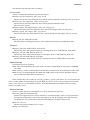
3.3.2.2. Targeted MD of the transition from closed to open conformation of F1 motor
Targeted MD reproduces conformation change of proteins much faster than the actual time scale by
applying force to the proteins atoms to promote the change. The following shows the input file of the productive
run applying the force to theβ-subunit atoms of F1 motor.
Productive run
The productive run of the Targeted MD is performed using the coordinate of the system after the
equilibration is complete. This example calculates the transition from closed to open conformation of the
28
3.Tutorials
β-subunit (total 5ns), with the following input file:
>cat run.in
[input]
mdat_file = ../molx/2JDI_BFsub_molx.mdat
crd_file = ../eq2/2JDI_BFsub_eq02.crd
restart = on
[nonbond]
cutoff = 10.0
[ewald]
d_grid = 1.1
[constraint]
rigid_body = hydrogen
[PT_control]
ensemble = NVT
temperature = 300
[init]
solute_molecule = 4
[md]
time_step = 2.0
step = 250000
remove_momentum = solute_rot
print_step = 500
trj_file = 2JDI_BFsub_rmsd01_001.trj
trj_step = 500
prop_file = 2JDI_BFsub_rmsd01_001.prop
prop_step = 5000
[output]
crd_file = 2JDI_BFsub_rmsd01_001.crd
pdb_file = 2JDI_BFsub_rmsd01_001.pdb
[restraint]
method = rmsd
k = 7300.0
pdb_file = 2JDI_AEsub.pdb
group = atom non_hydrogen 24B 601B
group = atom non_hydrogen 9F 474F
pdb_group = atom non_hydrogen 24B 601B
pdb_group = atom non_hydrogen 9F 474F
best_fit = on
rmsd = 5.62243
gradual_change_rmsd = 2500000 0.0
29
3.Tutorials
For the MARBLE input files, specify the parameters under each section indicated with "[ ]". The
specified contents are as follows. (For the items explained in the previous chapters, see the previous
descriptions.)
[init]
 solute_molecule = 4
In this simulation, the rotation of solvent molecules is stopped by specifying "remove_momentum =
solute_rot" in the [md] section. The "solute_molecule" command here specifies the number of the
solvent molecules of which rotation is to be stopped. This example specifies the number to 4 (i.e. F1 α-,
β-subunits, ATP, and Mg).
[restraint]
When performing Targeted MD in MARBLE, the force to apply to each atom is given as a restraining
force to maintain a RMSD value between the target and current structures. The restraint RMSD value is then
gradually changed to approach to the target structure (i.e. the value approaches zero).
 method = rmsd
Specifies the restraint method to the one with RMSD value between the current and target structures.
 k = 7300.0
In the method of restraint with RMSD values, atoms are restrained with the springs which vary
according to the RMSD values of the atoms between the current and target structures. This command
specifies the total value of the spring constant used in the system. This calculation example restrains
heavy atoms in B-chain residues 24 to 601 and those in F-chain residues 9 to 474, and the total count of
the restrained atoms is approximately 7300. Since this system example assumes the spring constant of
1(kcal•mol-1Å-2) per atom, the K value should be 7300.
 pdb_file = 2JDI_AEsub.pdb
Specifies the target structure. Since this example simulates the transition of the closed to open
conformation of the F1 motor β subunit, the 2JDI_AEsub.pdb (open conformation) is set to the target
structure.
 group = atom non_hydrogen 24B 601B
group = atom non_hydrogen 9F 474F
Specifies the atoms to be restrained with RMSD values. (Specify atoms in "2JDI_BFsub_eq02.crd"
specified in the input file.)
 pdb_group = atom non_hydrogen 24B 601B
pdb_group = atom non_hydrogen 9F 474F
Specifies the atoms used for calculating RMSD values at target structure (i.e. 2JDI_AEsub.pdb in this
example).
 best_fit = on
Modifies the overlap of the current and target structures with "best fit" during RMSD value
calculations. (This operation is for RMSD calculations and does not affect the current structure.)
 rmsd = 5.62243
Specifies the restraining RMSD value. (Here, "5.62243Å", the RMSD value between the closed
conformation and the target open conformation is specified.)
 gradual_change_rmsd = 2500000 0.0
Specifies the restraining RMSD value to overlap the target structure (i.e. RMSD=0) in 2,500,000 steps.
prop file
When executing the Target MD with the input file above, the content of the output prop file is as follows:
#1 TIME 2 TEMPERATURE 3 TOTAL_ENE 4 POTENTIAL 5 RMSD_ENE 6 RMSD 7 TARGET_RMSD
2.100000e+02 3.013549e+02 -3.196633e+05 -3.941214e+05 9.339044e-03 5.610054e+00 5.611185e+00
30
3.Tutorials
2.200000e+02 3.004271e+02 -3.196564e+05 -3.936027e+05 2.758408e-02 5.601884e+00 5.599940e+00
2.300000e+02 2.992376e+02 -3.196625e+05 -3.940014e+05 1.615850e-01 5.583991e+00 5.588695e+00
2.400000e+02 2.998921e+02 -3.196609e+05 -3.934682e+05 3.922606e-03 5.576718e+00 5.577451e+00
2.500000e+02 3.001248e+02 -3.196620e+05 -3.936488e+05 7.254864e-01 5.556237e+00 5.566206e+00
2.600000e+02 3.005848e+02 -3.196579e+05 -3.933531e+05 5.966773e-01 5.564002e+00 5.554961e+00
2.700000e+02 2.998154e+02 -3.196666e+05 -3.942913e+05 3.877468e-04 5.543486e+00 5.543716e+00
2.800000e+02 3.011331e+02 -3.196645e+05 -3.937764e+05 3.908584e-02 5.530157e+00 5.532471e+00
2.900000e+02 2.993740e+02 -3.196623e+05 -3.938691e+05 4.938038e-01 5.513002e+00 5.521226e+00
3.000000e+02 2.997662e+02 -3.196665e+05 -3.941785e+05 4.499579e-01 5.502130e+00 5.509981e+00
------------Omitted
------------5.140000e+03 3.020446e+02 -3.163080e+05 -3.928481e+05 1.319831e+03 4.926735e-01 6.746916e-02
5.150000e+03 2.994278e+02 -3.162387e+05 -3.930239e+05 1.319981e+03 4.814528e-01 5.622430e-02
5.160000e+03 3.012046e+02 -3.161688e+05 -3.924416e+05 1.368356e+03 4.779299e-01 4.497944e-02
5.170000e+03 3.007494e+02 -3.160989e+05 -3.927360e+05 1.435828e+03 4.772306e-01 3.373458e-02
5.180000e+03 2.995500e+02 -3.160180e+05 -3.922802e+05 1.462634e+03 4.701066e-01 2.248972e-02
5.190000e+03 2.998215e+02 -3.159517e+05 -3.928270e+05 1.523464e+03 4.680749e-01 1.124486e-02
5.200000e+03 3.000127e+02 -3.158740e+05 -3.925378e+05 1.564234e+03 4.629024e-01 0.000000e+00
The numbers in the columns from the left indicates calculation time, temperature, total energy, potential
energy, restraining energy, current RMSD value, and target RMSD value. The table above shows that the
RMSD values in the sixth column approach from the initial value 5.62243 to the target value 0.0. (For the initial
and target values, see the previous [restraint] section for input files.)
31
4.Execution Procedure for the molx and MARBLE (for K computer and FX10)
4. Execution Procedure for the molx and MARBLE (for K computer and
FX10)
For K computer and FX10, the molx and MARBLE are generated as execution files for computing nodes.
This chapter describes how to execute the molx and MARBLE on computing nodes, using the FX10 as an
example.
4.1. Execution procedure for the molx
The molx must be executed on computing nodes since it cannot execute on the login node.
Execute the molx in the batch mode, or first login to the computing node in the interactive mode and then
execute the program.
4.2. Execution procedure for MARBLE
This section describes how to perform parallel computation by specifying the necessary data, such as the
number of cell divisions, number of processes, three-dimensional specification of the processes, and grids for
PME method, using the two specification methods described in "3.1.5 Parallel computation in MARBLE".
Performing MARBLE calculations requires the following data as explained in "3.1.5 Parallel computation
in MARBLE":
(a) The number of cell divisions in the system in X, Y, and Z directions
(b) The number of processes used
(c) The number of processes arranged in X, Y, and Z directions
(d) The number of grids made by dividing the space at even intervals in X, Y, and Z directions to calculate
electrostatic interactions with PME (Particle Mesh Ewald) method
Further, the items (a) to (d) must be determined so that they satisfy the specific rules as described below:
The number of the processes to be used is the product of the numbers of the processes arranged in X, Y,
and Z directions.
To determine the number of cell divisions, satisfy the following items:
 (A)The minimum cell width must be (cutoff + 4.5)/2, where "cutoff" is specified in [nonbond]. For
example, when the cutoff is 9, the width is 6.75. When the cutoff is 10, the width is 7.25. Determine the
number of cell divisions based on the width larger than the minimum width for X, Y, and Z directions.
 (B)The number of cell divisions in each direction must be divisible by the number of the processes
arranged for that direction.
To determine the number of grids for PME in XYZ directions, satisfy the following items:
 (C)The grid intervals must be approximately 1.1Å or smaller.
 (D)The number of grids in each direction must be divisible by the number of the processes arranged for
that direction.
MARBLE provides the following two methods to specify the data (a) to (d). The sections below describe
the calculation procedure with each method:
32
4.Execution Procedure for the molx and MARBLE (for K computer and FX10)
4.2.1. Using d_grid
In this method, the user can easily specify all data necessary for parallel computation by only specifying
the number of processes for computation.
First, describe the shell script file (batch.sh) for executing a batch job, as follows:
#!/bin/sh
#PJM -L "rscgrp=debug"
#PJM -L "node=4x2x2"
#PJM - -mpi “proc=64”
#PJM -L "elapse=30:00"
#PJM –j
export OMP_NUM_THREADS=4
mpiexec /home/xxxx/marble-0.6/bin/marble.0.6.0_FX10 run01.in run01.out
The shell script file above performs hybrid parallel computation with the following parameters:
The number of nodes: 4x2x2 (#PJM –L “node=4x2x2”)
The number of processes: 64 (#PJM - -mpi “proc=64”)
The number of threads: 4 (export OMP_NUM_THREADS=4)
In this example, four processes are submitted to each node. The four processes are then further divided in
the way that the numbers of the processes in x, y, and z directions are equal.
Next, as explained in chapter 3, describe as follows in the [ewald] section in the input file for MARBLE
execution (run01.in):
[ewald]
d_grid = 1.1
Then, based on the system box size and d_grid value, the program determines the number of grids for
PME in each direction, and according to the specified number of processes, automatically calculates the number
of the cells and processes in each direction, and performs computation.
In this method, however, since MARBLE uses the d_grid and box size data for computation, the grid size
for PME may change during the computation in case that the size of the box is changed, as in NPT ensemble.
4.2.2. Specifying the data directly
Another method is to specify the data (a) to (d) directly in input files so that the items (A) to (D) above
are satisfied.
First, describe the shell script file (batch.sh) for executing a batch job, as follows:
#!/bin/sh
#PJM -L "rscgrp=debug"
#PJM -L "node=2x2x4"
#PJM --mpi "proc=64"
33
4.Execution Procedure for the molx and MARBLE (for K computer and FX10)
#PJM -L "elapse=30:00"
#PJM -j
export MBL_PE_NODE=2x2x1
export OMP_NUM_THREADS=4
mpiexec /home/c74000/marble-0.6/bin/marble.0.6.0_FX10 run01a.in run01a.out
The shell script file above performs hybrid parallel computation with the following parameters:
The number of nodes: 16 (#PJM –L “node=2x2x4”)
The number of processes: 64 (#PJM - -mpi “proc=64”)
The number of threads: 4 (export OMP_NUM_THREADS=4)
Here, the number of processes for a node is four. If no particular setting is made, the four processes are
further divided in the way that the numbers of processes in x, y, and z directions are equal.
However, if the user wishes to specify the division method manually, the user can specify as follows in
the shell script above:
export MBL_PE_NODE=2x2x1
Then the three-dimensional division of the processes on each node is set to 2x2x1. With this, the
three-dimensional division of the processes for nodes and that of the processes within the node are set to 2x2x4
and 2x2x1, respectively. The three-dimensional division for the entire computation process thus becomes
4x4x4.
Further, the following shows a part of the description of the input file (run01a.in) for MARBLE
execution.
---------------------[nonbond]
cutoff = 10.0
n_cell = 8 8 8
n_pe = 4 4 4
[ewald]
method=PME
grid=72 72 72
----------------------
Here, the section [nonbond] specifies "cutoff = 10.0".
(This means the minimum cell width is 6.75 from the formula mentioned above.)
Note here that the size of lysozyme box is 72.66Å on each side (see the output of the molx execution in
3.2.2). We therefore set the number of divisions for cells, processes, and PME grids in X,Y, and Z directions to
8x8x8, 4x4x4, and 72x72x72, respectively.
34
5.Command Reference
5. Command Reference
This chapter describes the commands used for the molx and MARBLE. Each command is indicated in
bold type in the descriptions.
5.1. The molx
Usage (see 3.1.1)
molx input file
Example
molx molx.in
For the content of input files for actual calculation, see "3.2 Constructing the system with the molx".
5.1.1. Force field
These commands specify the files for using the CHARMM force field (i.e. top files, par files, and toppar
files).
charmm_top_file
Specifies the CHARMM top file (default value: none). A maximum of five top files can be specified.
Usage: charmm_top_file file name
Example: charmm_top_file top_all27_prot_na.rtf
charmm_par_file
Specifies the CHARMM par file (default value: none). A maximum of five top files can be specified.
Usage: charmm_par_file file name
Example: charmm_par_file par_all27_prot_na.rtf
charmm_toppar_file
Specifies the CHARMM par file (default value: none). A maximum of five toppar files can be specified.
Usage: charmm_toppar_file file name
Example: charmm_toppar_file toppar_all22_prot_pyridines.str
5.1.2. Input
This command specifies the structural information of target molecules as an input. Basically, a pdb file is
used for the specification. The user can also specify protein primary structures (i.e. amino acid sequences) to
perform linear peptide calculation.
input_pdb_file
Specifies a pdb file of proteins, etc. used for calculation (default value: none).
Usage: input_pdb_file file name
Example: input_pdb_file 6lYZ.pdb
5.1.3. Output
These commands output the files necessary for MARBLE simulations, such as crd and mdat files of the
system constructed in the molx and pdb file of the constructed system.
output_mdat_file
Specifies an mdat file for the system constructed in the molx (default value: none).
Usage: output_mdat_file file name
35
5.Command Reference
Example: output_mdat_file 6lyz_w.mdat
output_crd_file
Specifies a crd file for the system constructed in the molx (default value: none).
Usage: output_crd_file file name
Example: output_crd_file 6lyz_w.crd
output_pdb_file
Specifies a pdb file of the entire system constructed in the molx (default value: none).
Usage: output_pdb_file file name
Example: output_pdb_file 6lyz_w.pdb
5.1.4. Model building
These commands set up the calculation target molecule.
renumber_residue
Renumbers residue numbers (default number: ).
Usage: renumber_residue {on|off}
Example: renumber_residue on
rename_residue
Changes the name of a specific residue described in input files (default value: none?)
Usage: rename_residue residue number＋chain_ID new residue name
Example: rename_residue 15A HSE
bond_length_limit
Specifies the upper limit of interatomic bond length in input files (default value: ??).
Usage: bond_length_limit upper limit of bond length
Example: bond_length_limit 5
patch_ter
Modifies the data of N- and C-terminuses of proteins in input files using the patch defining several
terminuses in the CHARMM force field.
Usage: patch patch name residue number (+chain_ID)
Example: patch_ter NTER 23B
patch
Modifies the protein data in input files using several patches defined in the CHARMM force field.
Usage: patch patch name residue number 1 (+chain_ID) ……
Example: patch DISU 64A 80A
Note:
The syntax of the patch command, such as the number of residues to specify, varies depending on the
patch type. For details, refer to the patch information of the CHARMM force field.
alias
Changes the name of atoms or residues in input files.
(Not as in "rename_residue", this command is applied to all atoms or residues found in the relevant
input file.)
36
5.Command Reference
Usage: alias old name new name
Example: alias CD CD1
5.1.5. System building
These commands set up the solvent environment where the target molecule is placed. In this section, the
settings are made in order of "Creating a box", "Adding water", and "Adding ions".
Creating a box
MARBLE performs calculation in solvent environment using periodic boundary conditions. Therefore it
is first necessary to define a box on which to specify the periodic boundaries.
box
Used to manually define a box. Use this command when the size of the box is already determined.
(default value: none. However, α, β, and γ are set to 90º if not specified.)
Usage: box x y z α β γ
Example: box 169.10 169.10 170.27
align_axis
Aligns the molecule axis with the specified direction to the box. For alignment directions, three options of
"on", "z", and "diagonal" are available (default value: none). See below for the options:
"on": Aligns the molecule's longest principal axis of inertia with x axis.
"z": Aligns the molecule's longest principal axis of inertia with z axis.
"diagonal": Places the molecule so that its longest principal axis of inertia is aligned with the box
diagonal line.
Usage: align_axis {normal|z|diagonal}
Example: align_axis diagonal
solvent_cube
Specicfies the box shape as a cube. If this is "on", the program defines a cube by determining the side of
the cube according to the distance from the solvent surface defined in "solvent_buffer" (default vavlue: none).
Usage: solvent_cube on
Example: solvent_cube on
Adding water
After the box is defined, generate water molecules (solvent) used for the calculation in the box.
solvent_pdb_file
Specifies the pdb file of the solvent molecules to be placed in the box. Use wat216.pdb in usual cases
(default value: none).
Usage: solvent_pdb_file file name
Example: solvent_pdb_file wat216.pdb
solvent_excluded_layer
Defines the thickness of the surface layer of the solute molecule where the solvent is excluded (default
value: 0Å).
Usage: solvent_excluded_layer layer thickness (Å)
Example: solvent_excluded_layer 2
37
5.Command Reference
solvent_buffer
Specifies the minimum thickness of the layer from the solute to the box wall (default value: 10Å).
Usage: solvent_buffer thickness of solvent molecule layer (Å)
Example: solvent_buffer 15
Adding ions
After water is generated, generate ions so that the total system charge is neutralized. Generate ions by
replacing water molecule coordinates.
ion
Specifies the type of ions added to the system (default value: none).
Usage: ion cation name anion name
Example: ion SOD CLA
Note:
The names of cation and anion used here must be those in the CHARMM force field. Be sure to describe
the names of cation and anion accurately in the specified order. If the names or their order is inaccurate, the
molx performs calculation on wrong ions and a significant error may occur in the total charge. Only monovalent
ions can be used for anions and cations.
ion_placement
Specifies how to place ions to "random" or "energy". The former generates ions randomly and the latter
generates ions in the positions where the energy is minimized (default: random).
Usage: ion_placement {random|energy}
Example: ion_placement energy
ion_cutoff
Specifies the cutoff distance for ions. Specify this command when "ion_placement" is "energy"
(default value: 10Å).
Usage: ion_cutoff cutoff length (Å)
Example: ion_cutoff 7
ion_density
Generates the ions specified with "ion" command so that the ion density becomes the specified value
(default value: 0mM).
Usage: ion_density ion density (mM)
Example: ion_density 4
5.2. MARBLE
Usage (see 3.1.1)
marble input file output file
Example
marble run.in run.out
For the content of input files for actual calculation, see "3.2 Constructing the system with the molx".
38
5.Command Reference
5.2.1. [input]
This section specifies the input files used for MARBLE calculations.
mdat_file
Loads the .mdat file data created in the molx.
Usage: mdat_file = file name
Example: mdat_file = ../molx/protein.mdat
crd_file
Loads the xyz coordinate data of each atom from .crd files.
Usage: crd_file = file name
Example: crd_file = run001.crd
restart
Use this command when performing a molecular simulation with separate input files and when inheriting
the ensemble and velocity data in the previous calculation. To specify .crd file data toinherit, use the following
keywords:
on: Uses all data in .crd files (default value: none).
V: Velocity
B: Periodic boundary box data
E: Energy
In particular, when restarting calculation with a different ensemble, select the keywords V, B, and E above,
and specify the desired ensemble with [PT_control] section described below. (This operation has the same
result as that of specifying "initialize=on" in [PT_control].)
Usage: restart = {on|V|B|E}
Example: restart = VB
5.2.2. [output]
Specifies the output file used for MARBLE calculations.
crd_file
Outputs .crd files containing the calculated final structure.
Usage: crd_file = file name
Example: crd_file = run001.crd
pdb_file
Outputs .pdb files containing the calculated final structure.
Usage: pdb_file = file name
Example: pdb_file = run001.pdb
5.2.3. [init]
This section specifies the initial setting of calculation parameters.
temperature
Specifies the initial temperature of the system (default value: none).
Usage: temperature = specified temperature
Example: temperature = 300
39
5.Command Reference
Use this command to define the initial velocity of each atom at calculation start. It is unnecessary to set
this command when continuing calculation with another input file, such as a .crd file for completed simulations.
solute_molecule
Specifies the number of solute molecules in the system (default value: none).
Usage: solute_molecule = number of solute molecules
Example: solute_molecule = 3
5.2.4. [restraint]
This section performs the various settings for restraining atoms.
method
Specifies a method to restrain atoms. The method can be specified with the following keywords:
position_harmonic: Restrains the specified group of atoms to the specified coordinates with springs.
rmsd: Restrains the specified group of atoms so that the RMSD (Root Mean Square Displacement) values
between the atoms and specified coordinates are satisfied.
The following describes the parameters of the restraining method specified in "method":
5.2.4.1. position_harmonic
When specifying "position_harmonic" in "method", specify the following commands:
(1) Specifying coordinate files to be referred
Specify the coordinate file used as a reference with the command below. The user can specify either a crd
file or pdb file. Use the command crd_file or pdb_file according to the file type.
crd_file
Specifies a crd file to which to refer to select atoms to be restrained.
Example: crd_file = test.crd
pdb_file
Specifies a pdb file to which to refer to select atoms to be restrained.
Example: pdb_file = test.pdb
(2) Specifying group of atoms to be restrained
When using a crd file as a coordinate reference, use "group" command. When using a pdb file, use
"group_pdb" command.
group
Specifies a group of atoms to be restrained in the crd structure loaded with a crd file.
Usage: group = atom selected atom type first residue end residue
Example: group = atom non_hydrogen 24B 601B
pdb_group
Specifies a group of atoms to be restrained in the pdb structure loaded with a pdb file.
Usage: pdb_group = atom selected atom type first residue end residue
Example: pdb_group = atom non_hydrogen 24B 601B
40
5.Command Reference
(3) Setting restraint parameters
k
Specifies the spring constant of a potential function applied to each atom to be restrained.
Usage: k = spring constant (kcal/mol/ang^2)
Example: k = 1.0
gradual_change_k
Gradually changes the spring constant specified with "k" command to the target value with specified
number of steps. Use this command to gradually apply or remove restraint during simulations.
Usage: gradual_change_k = number of steps target spring constant
Example: gradual_change_k = 50000 0
5.2.4.2. rmsd
When specifying "rmsd" in "method", set up the following commands:
(1) Specifying coordinate files to be referred (see 5.2.4.1 position_harmonic)
(2) Specifying group of atoms to be restrained (see 5.2.4.1 position_harmonic)
(3) Specifying restraint parameters
rmsd
Applies restraint so that the rmsd value specified with this command is satisfied.
Usage: rmsd = target rmsd value (Å)
Example: rmsd = 3.5
gradual_change_rmsd
Gradually changes the value specified in "rmsd" to the target value with specified number of steps. (Use
this command for Targeted MD. See 3.3.2.2.)
Usage: gradual_change_rmsd = number of steps target rmsd value
Example: gradual_change_rmsd = 500000 0
best_fit
Fits the snap shot structure to the target coordinate when checking the restraint rmsd in each step of
simulation.
Usage: best_fit = on
k
Specifies the spring constant of a potential function applied to each atom to be restrained.
Usage: k = spring constant (kcal/mol/ang^2)
Example: k = 1.0
5.2.5. [constraint]
This section performs the settings to handle groups of atoms bonded with hydrogen (methyl groups, etc.,)
as rigid-body. Using this option allows decreasing the simulation time step to approximately 2fs since hydrogen
bond vibration can be neglected.
rigid_body
Specifies the target atom to be handled as rigid-body (default value: none).
Example: rigid_body = hydrogen
41
5.Command Reference
5.2.6. [PT_control]
This section specifies the system ensemble, as well as temperature and pressure control.
ensemble
Specifies the ensemble for the system calculation (default value: NVT).
Usage: ensemble = {NVT|NPT|NVE}
Example: ensemble = NPT
initialize
Changes the system ensemble (default value: none).
Usage: initialize=on
Note:
Use this command to change ensemble (for example, from NVT to NPT) when restarting calculation and
continuing the previous simulation. Note that if this command is used, the data obtained from the previous
calculation in .crd files will be reset (except for coordinate sets). Use this command only when it is necessary to
change the ensemble from the previous calculation.
method
Specifies how to control temperature and pressure (default value: extended_system).
Usage: method = {extended_system|rescaling}
Example: method = rescaling
Note:
The "rescaling" is available only for the NVT ensemble.
temperature
Specifies the system temperature (default: 298.15 (k)).
Usage: temperature = set temperature (K)
Example: temperature = 310
pressure
Specifies the system pressure (default: 1 (atm))
Usage: pressure = set pressure (atm)
Example: pressure = 1.0
gradual_change_T
Changes the temperature to the target value with specified time steps (default value: the number of
steps=0, target temperature=the "temperature" value).
Usage: gradual_change_T = number of steps target temperature (K)
Example: gradual_change_T = 10000 300 (changing temp. to 300(k) in 10000 steps)
5.2.7. [nonbond]
This section specifies the settings necessary for calculating non-bonded interactions in the system.
cutoff
Specifies the cutoff radius for non-bonded interactions (default value: 9.0Å)
Usage: cutoff = cutoff radius (Å)
Example: cutoff = 10
42
5.Command Reference
n_cell (unnecessary when d_grid is specified in the [ewald] section)
Specifies how to define cells on the box during parallel computation.
Usage: n_cell = (n_cell)x (n_cell)y (n_cell)z
(n_cell)x,y,z: number of cells in each component (integer)
Example: n_cell = 20 20 20
Note:
When specifying the cells, refer to the minimum cell width obtained by (cutoff + 4.5)/2. For example,
when the cutoff=9(Å), the width is 6.75(Å). If the width of the box and the cutoff is 64Å and 9Å, respectively,
the minimum cell width is 64/6.75=9.481. In this example, the number of the cells should be 9 or smaller.
n_pe (unnecessary when d_grid is specified in the [ewald] section)
Specifies how to divide the process for parallel computation into spatial divisions.
Usage: n_pe = (n_pe)x (n_pe)y (n_pe)z
(n_pe)x,y,z: number of cells in each component (integer)
Example: n_pe = 10 10 10
Note:
The specified processes must satisfy the following rules:
The values (n_cell)x, (n_cell)y, and (n_cell)z must be divisible by (n_pe)x, (n_pe)y, and (n_pe)z,
respectively.
The number of grids in x, y, and z components specified in [ewald] section must be divisible by (n_pe)x,
(n_pe)y, and (n_pe)z, respectively.
The number of total processes used for the calculation must be the product of the number of each
component of x, y, and z, namely, (n_pe)x*(n_pe)y*(n_pe)z.
5.2.8. [ewald]
This section performs the settings on the PME method (Particle Mesh Ewald) to calculate long-range
electrostatic interactions in the system.
grid
Specifies the number of grids on the system box in X, Y, and Z directions (default value: none).
Usage: grid = (n_grid)x (n_grid)y (n_grid)z
(n_grid)xyz: number of grids in XYZ directions of the box (integer)
Example: grid = 20 20 20
Note:
The grid interval must be approximately 1.1Å or smaller.
d_grid
Specifies the intervals of the grids defined on the system box (default value: none).
Usage: d_grid = grid interval (Å)
(The grid interval must be approximately 1.1Å or smaller.)
Example: d_grid = 1.1
43
5.Command Reference
Note:
When specifying "d_grid", it is unnecessary to specify a "grid" value. Once the user defines "d_grid"
value, MARBLE automatically determines the number of grids in X, Y, and Z directions according to the size of
the system box. In addition, MARBLE also determines "n_cell" and "n_pe" values, which is usually to be
defined in [nonbond]. Since it is troublesome to find "n_cell" and "n_pe" values satisfying the conditions
described in the [nonbond] section, it is recommended to use "d_grid" in usual MD calculations.
5.2.9. [min]
This section performs the settings on energy minimization calculations.
step
Specifies the number of steps to perform energy minimization with the steepest descent method (default
value: none).
Usage: step = number of steps
Example: step = 1000
print_step
Specifies the frequency of outputting energy values obtained with energy minimization calculation, using
the number of steps (default value: 1).
Usage: print_step = number of steps
Example: print_step = 10
cg_step
Specifies the number of steps to perform energy minimization with the conjugate gradient method
(default value: 0).
Usage: cg_step = number of steps
Example: cg_step = 1000
Note:
When both "step" and "cg_step" are specified, the steepest descent method is first performed with the
number of steps specified in "step", and the conjugate gradient method is performed with the number of steps
in "cg_step".
grad
Specifies the gradient value to judge the convergence of energy minimization (default value: 1.0e-4).
Usage: grad = gradient value
Example: grad = 2.0e-4
5.2.10. [md]
This section performs the settings on molecular dynamics simulations.
time_step
Specifies the time increment per step in molecular dynamic simulations.
Usage: time_step = time increment per step (fs)
Example: time_step = 2
step
Specifies the number of steps for molecular dynamics simulations (default value: 0).
Usage: step = number of steps
Example: step = 500000
44
5.Command Reference
prop_file
Specifies the data output file (prop file) for molecular dynamics simulations (default value: none).
Usage: prop_file = file name
Example: prop_file = md1.prop
prop_step
Specifies the frequency of outputting data onto prop files (default value: 100).
Usage: prop_step = number of steps
Example: prop_step = 1000
trj_file
Specifies the file (trj files) to output trajectories of molecular dynamics simulations (default value: none).
Usage: trj_file = file name
Example: trj_file = md1.trj
trj_step
Specifies the frequency of outputting data onto trj files (default value: 100).
Usage: trj_step = number of steps
Example: trj_step = 1000
trj_output
Specifies the information to be output in trj files (default value: XB).
Usage: trj_output = {X|V|B}(X: coordinate, V: velocity, B: box data)
Example: trj_output = XB
print_step
Specifies the frequency of outputting the energy values obtained with molecular dynamics simulations,
using the number of steps (default value: 1).
Usage: print_step = number of steps
Example: print_step = 10
remove_momentum
Specifies whether or not to remove translation and rotation of target proteins during molecular dynamics
simulations.
Usage: remove_momentum ={off|all|all_rotation|solute_translation|solute_rotation}
Example: remove_momentum = solute_rotation
45