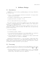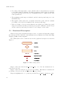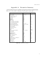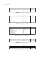
1
Claudia User Manual Daniel Finch, Nick Lioutas and Ross Kyprianou Electronic Warfare and Radar Division Defence Science and Technology Organisation DSTO–GD–0554 ABSTRACT This document is the user manual for version 1.0 of the generic maritime radar performance model ‘Claudia’. Claudia computes the target detection performance of radars in maritime environments. APPROVED FOR PUBLIC RELEASE DSTO–GD–0554 Published by DSTO Defence Science and Technology Organisation PO Box 1500 Edinburgh, South Australia 5111, Australia Telephone: Facsimile: (08) 8259 5555 (08) 8259 6567 © Commonwealth of Australia 2008 AR No. AR-014-326 October, 2008 APPROVED FOR PUBLIC RELEASE ii DSTO–GD–0554 Claudia User Manual Executive Summary The EWRD Microwave Radar Branch has undertaken to establish a flexible framework for radar modelling to maximise code reusability. The framework is focussed on the parametric modelling of maritime radars, and provides the ability to develop a complete system from individual components to conduct performance evaluation of maritime radar systems. iii DSTO–GD–0554 iv DSTO–GD–0554 Authors Daniel Finch Electronic Warfare and Radar Division Daniel Finch works in radar modelling and analysis in EWRD, DSTO. He joined DSTO in 2003 after completing degrees in Mathematics and Electrical Engineering at the University of Wollongong Nick Lioutas Electronic Warfare and Radar Division Nick Lioutas currently works in Electronic Warfare and Radar Division, DSTO. His work involves the analysis and modelling of radar system performance. He completed a BSc(Hons) degree at the University of Adelaide in 1981. Ross Kyprianou Electronic Warfare and Radar Division Ross Kyprianou currently works in EWRD in the area of sea clutter modelling after graduating from the University of Adelaide in 1985 with a Bachelor of Science and a Post Graduate Diploma in Computer Science in 1987. v DSTO–GD–0554 vi DSTO–GD–0554 Contents 1 Introduction 1 2 Claudia Capabilities 1 3 Input Files 3 3.1 Introduction . . . . . . . . . . . . . . . . . . . . . . . . . . . . . . . . . . 3 3.1.1 XML Syntax . . . . . . . . . . . . . . . . . . . . . . . . . . . . . . 3 3.2 Claudia XML Elements and Conventions . . . . . . . . . . . . . . . . . . 3 3.3 The Radar File . . . . . . . . . . . . . . . . . . . . . . . . . . . . . . . . . 4 3.3.1 Sample Radar File Listing . . . . . . . . . . . . . . . . . . . . . . 5 3.3.2 Description of Parameters . . . . . . . . . . . . . . . . . . . . . . 6 3.4 3.5 3.6 3.7 3.8 4 The Platform File . . . . . . . . . . . . . . . . . . . . . . . . . . . . . . . 10 3.4.1 Sample Platform File Listing . . . . . . . . . . . . . . . . . . . . 10 3.4.2 Description of Parameters . . . . . . . . . . . . . . . . . . . . . . 10 The Target File . . . . . . . . . . . . . . . . . . . . . . . . . . . . . . . . . 11 3.5.1 Sample Target File Listing . . . . . . . . . . . . . . . . . . . . . . 11 3.5.2 Description of Parameters . . . . . . . . . . . . . . . . . . . . . . 11 The Environment File . . . . . . . . . . . . . . . . . . . . . . . . . . . . . 12 3.6.1 Sample Environment File Listing . . . . . . . . . . . . . . . . . . 12 3.6.2 Description of Parameters . . . . . . . . . . . . . . . . . . . . . . 12 The Scenario File . . . . . . . . . . . . . . . . . . . . . . . . . . . . . . . . 14 3.7.1 Sample Scenario File Listing . . . . . . . . . . . . . . . . . . . . . 14 3.7.2 Description of Parameters . . . . . . . . . . . . . . . . . . . . . . 14 The Configuration File . . . . . . . . . . . . . . . . . . . . . . . . . . . . . 15 3.8.1 Sample Configuration File Listing . . . . . . . . . . . . . . . . . . 15 3.8.2 Description of Parameters . . . . . . . . . . . . . . . . . . . . . . 15 Running Claudia 15 4.1 System Requirements . . . . . . . . . . . . . . . . . . . . . . . . . . . . . 15 4.2 Installing the Software . . . . . . . . . . . . . . . . . . . . . . . . . . . . . 16 4.3 Running Claudia . . . . . . . . . . . . . . . . . . . . . . . . . . . . . . . . 16 4.4 Claudia Outputs . . . . . . . . . . . . . . . . . . . . . . . . . . . . . . . . 17 4.4.1 find detection range . . . . . . . . . . . . . . . . . . . . . . . . . . 17 vii DSTO–GD–0554 5 6 7 4.4.2 plot detection probability . . . . . . . . . . . . . . . . . . . . . . 17 4.4.3 find detection probability 4.4.4 plot pd rcs . . . . . . . . . . . . . . . . . . . . . . . . . . . . . . . 18 4.4.5 plot range rcs . . . . . . . . . . . . . . . . . . . . . . . . . . . . . 19 4.4.6 plot required rcs . . . . . . . . . . . . . . . . . . . . . . 17 . . . . . . . . . . . . . . . . . . . . . . . . . . . 19 Software Design 21 5.1 Introduction . . . . . . . . . . . . . . . . . . . . . . . . . . . . . . . . . . 21 5.2 Processing . . . . . . . . . . . . . . . . . . . . . . . . . . . . . . . . . . . . 21 5.3 Functional Description . . . . . . . . . . . . . . . . . . . . . . . . . . . . . 22 Radar Range Equation 26 6.1 Target . . . . . . . . . . . . . . . . . . . . . . . . . . . . . . . . . . . . . . 26 6.2 Propagation . . . . . . . . . . . . . . . . . . . . . . . . . . . . . . . . . . . 26 6.3 Signal-to-Interference Ratio . . . . . . . . . . . . . . . . . . . . . . . . . . 27 6.4 Surface Clutter . . . . . . . . . . . . . . . . . . . . . . . . . . . . . . . . . 27 6.5 Volume Clutter . . . . . . . . . . . . . . . . . . . . . . . . . . . . . . . . . 28 6.6 Noise . . . . . . . . . . . . . . . . . . . . . . . . . . . . . . . . . . . . . . 28 6.7 Probability of Detection . . . . . . . . . . . . . . . . . . . . . . . . . . . . 28 Planned Enhancements 28 References 29 Appendix A viii Parameter Summary 31 DSTO–GD–0554 1 Introduction EWRD’s Microwave Radar (MR) Branch has undertaken to establish a flexible framework for radar modelling to maximise code re-usability. Claudia is based on a software model previously generated within MR Branch, and is focussed on the parametric modelling of ship-borne surface search and airborne maritime radars. The framework also provides the ability to develop a complete system from individual user-developed components to conduct performance evaluation of maritime radar systems. Claudia computes the detection performance of a maritime radar within its operating environment against designated targets. It is written in the MATLAB programming language and is comprised of a number of software modules and data structures, each representing different components of the modelled scene and detection process. All software modules are designed to be easily interchangeable when more precise or higher level components are developed. The model inputs are divided into six components. Each component is defined by a number of user-defined parameters which are readily modifiable. The components are: • the radar • radar platform dynamics • a target • the operating environment • scenario • configuration. The software has six pre-defined methods of presenting results from detection performance calculations. The design is such that new methods can be added easily as required. This document is a description and user guide for operating Claudia version 1.0. It describes software installation, setting up the input files, and running the model. Included in this document is a functional description to assist with a more informed use of the software and a description of the equations on which the model is based. 2 Claudia Capabilities This section outlines Claudia’s current capabilities regarding calculation of the detection performance of maritime radars. However, Claudia is in reality a modelling framework, so the following attributes are not necessarily limiting. These capabilities are summarised as follows: • Coherent (pre-detection) and non-coherent (post-detection: video or binary) integration of pulses and pulse bursts. 1 DSTO–GD–0554 • Ability to evaluate detection thresholds and probability of detection for surface clutter with variable amplitude distributions, and a Rayleigh distribution of noise and volume clutter. • Detection thresholds and probabilities of detection can be calculated for targets with Swerling case 0, 1, 2, 3 and 4 radar cross section fluctuations. • The target is represented as a point scatterer with a specified radar cross section at a specified height above sea level. • The Georgia Institute of Technology (GIT) sea clutter model [1] is used to compute the mean sea clutter reflectivity in the frequency range 1 - 100 GHz. • Radar propagation may be set as either free space (i.e. direct path only) or multipath (i.e. direct and reflected path). Both the free and multi-path propagation models use a modified earth radius (effective earth radius factor of 4/3) to account for the refraction of the radar signals by the troposphere. The maximum range of the target cannot exceed the maximum range of the interference region. Beyond the interference region, it is assumed that multi-path propagation is not valid. • The Gaussian function is used to define the main-lobe pattern of the radar antenna. • The impact of rain attenuation and reflectivity on detection performance is calculated. Rain attenuation calculations use the ITU recommendation [2]. This algorithm is limited to horizontal and vertical polarisations, and transmitter frequencies in the range 1 - 400 GHz. Rain reflectivity is computed for transmitter frequencies in the range 3 - 140 GHz and rain rates up to 16 mm/hr using tables from Nathanson [3]. • Water vapour density, absolute temperature and dry air pressure profiles are calculated, using the ITU recommendation [4], as a function of height, operating latitude and the season of the year. These values are used to calculate the clear weather atmospheric attenuation. • A uniform sea surface, having the same sea-state and wave direction at all locations, is assumed. • The region of rain is represented as a rectangular cell of finite dimension. The modelling outcomes from Claudia are presented to the user via one of the following six outputs: • detection probability of a target at a specified range • detection range of a target (for a given probability of detection) • a plot of probability of detection against detection range • a plot of the minimum required RCS versus range so that a user defined detection probability is reached • a plot of detection range against a predefined set of RCS values • a plot of detection probability against RCS at a user defined range. 2 DSTO–GD–0554 3 3.1 Input Files Introduction This section describes the format and parameters of the six components that drive the radar model. Each component is defined in a separate input file, using the XML syntax for the reasons outlined in Section 5. The components are named ‘Radar’, ‘Platform’, ‘Target’, ‘Environment’, ‘Scenario’ and ‘Configuration’. 3.1.1 XML Syntax A brief outline of the EXtensible Markup Language (XML) syntax is provided below. More information on the XML syntax is available from computing texts, or online tutorials such as W3Schools [5]. XML is a method of expressing data in a hierarchical tree structure. The top of the tree is the ‘root element’, under which ‘child elements’ are placed. All elements can have subelements (child elements). This structure is demonstrated below. <root> <child1> <subchild> ... </subchild> </child1> <!-- this is a comment <child2 key1="value1" /> </root> --> Elements are enclosed in opening and closing tags. As shown above, the opening tag begins with the angled bracket ‘<’ and is followed by a tag name, any number of paired attribute names (e.g. ‘key1’) and attribute values (e.g. ‘value1’) and finally an angled bracket ‘>’. The closing tag is constructed with the angled bracket, tag name, and the closing angled bracket ‘/>’. In the case of empty elements, it is possible combine the opening and closing tags (e.g. ‘child2’ above). Note that tag names are case sensitive and must not contain spaces. As shown, XML syntax requires the attribute names and their corresponding values be separated by an ‘=’, and attribute values be enclosed by double quotes. Attribute names are not quoted. XML files may also contain any number of comment lines. The comments are enclosed within an opening tag of ‘<!--’ and closing tag ‘-->’ as shown above. Comment lines can be inserted anywhere within the XML except within the opening and closing tags of elements. 3.2 Claudia XML Elements and Conventions The root element of each file has the same name as the component represented in the file (e.g. ‘<Radar>’ for a Radar component). All parameters of this component are 3 DSTO–GD–0554 then entered as child elements with the two attributes ‘value’ and ‘units’. Order of the parameters within the file is not important. Parameter names are case sensitive, however inputs for value and units are not. Parameters that are dimensionless may either exclude the units attribute, or set the unit to ‘NA’. The exception to this is parameters that are commonly expressed in decibels, in which case the units are set to ‘dB’ or ‘absolute’. Parameters that require character or string inputs should include single quotes (e.g. value="‘binary’"). It is possible to enter a valid MATLAB expression as the value of a parameter (e.g. value="sin(3*pi/2)"). All parameters for the component must be included in the input file, however the value attribute may be set as ‘NaN’ (MATLAB’s IEEE representation of ‘not a number’) in the following two cases: • the parameter is optional, in which case a default value will be used • the parameter is not required for calculations – the parameter is reserved for a future version of the software and not used in the current version – the parameter is a member of a subset of parameters, exactly one of which is required – the parameter is not required for the processing options selected. 3.3 The Radar File The radar file includes the parameter names and values for describing the radar’s transmitter, receiver, antenna and signal processing components. A typical listing is provided in Section 3.3.1. The structure of the radar file may be divided into ‘modes’ to describe radar parameters that pertain to the radar’s various operating modes. This is achieved using a ‘Mode’ element, having a value attribute corresponding to the mode’s name. When using modes, parameters that are common to all modes are entered directly below the ‘Radar’ tag, and those for the specific mode are entered as child elements of the mode. This structure is demonstrated in the sample file listing. The radar file is named by convention, rdr radarname.xml, where radarname is the name of the radar being described (e.g. rdr aps115.xml), but this convention is not enforced. 4 DSTO–GD–0554 3.3.1 Sample Radar File Listing <Radar> <TxPeakPower value="143000" units="W"/> <TxFrequency value="9.05e9" units="Hz"/> <TxLineLoss value="3.0" units="dB"/> <AntennaTilt value="0.5" units="deg"/> <RadomeLoss value="1" units="dB"/> <TxAntennaGain value="30" units="dB"/> <RxAntennaGain value="30" units="dB"/> <AzimuthBeamwidth value="2.5" units="deg"/> <ElevationBeamwidth value="9.9" units="deg"/> <Polarisation value="‘H’"/> <RxNoiseFigure value="9.5" units="dB"/> <RxLineLoss value="3.0" units="dB"/> <NonCoherentIntegration value="‘binary’"/> <BinaryN value="7"/> <BinaryM value="3"/> <AntennaLookDirection value="30" units="deg"/> <PulseCompressionRatio value="1.0"/> <CoherentIntegrationGain value="0" units="dB"/> <TotalSignalProcessingLosses value="1.0" units="dB"/> <NoPulseBursts value="NaN"/> <NoPulsesPerBurst value="NaN"/> <CoherentIntegrationTime value="NaN" units="s"/> <CIFSurface value="1.0"/> <CIFVolume value="1.0"/> <BeamShapeLoss value="NaN" units="dB"/> <Mode value="A"> <PRF value="1600" units="Hz"/> <ScanRate value="12" units="rpm"/> <PulseWidth value="0.5e-6" units="s"/> <MaximumDisplayRange value="64 * 1852" units="m"/> <RxNoiseBandwidth value="2.0e6" units="Hz"/> </Mode> <Mode value="B"> <PRF value="400" units="Hz"/> <ScanRate value="6" units="rpm"/> <PulseWidth value="2.5e-6" units="s"/> <MaximumDisplayRange value="128 * 1852" units="m"/> <RxNoiseBandwidth value="0.4e6" units="Hz"/> </Mode> </Radar> 5 DSTO–GD–0554 3.3.2 Description of Parameters There are thirty parameters for the radar file, these are listed in alphabetical order below. 3.3.2.1 AntennaLookDirection AntennaLookDirection is the azimuth look direction of the radar antenna, and is specified in degrees or radians clockwise from true north. The target is also assumed to be on this bearing. 3.3.2.2 AntennaTilt This is the elevation angle of the radar antenna bore-sight axis with respect to the horizontal. AntennaTilt is specified in degrees below the horizontal (i.e. if the bore-sight axis is tilted above the horizontal, AntennaTilt will be negative).This parameter is used in the calculation of the antenna’s voltage gain. 3.3.2.3 AzimuthBeamwidth AzimuthBeamwidth is the average of the transmit and receive antenna one-way 3 dB beamwidth in azimuth. The value may be entered in degrees or radians. 3.3.2.4 BeamShapeLoss BeamShapeLoss is the loss resulting from the non-uniform gain within the 3dB beamwidth of the antenna as it scans past the target. If BeamShapeLoss is set to NaN, it is calculated from the number of pulses integrated within the 3dB beamwidth of the antenna. Otherwise, it can be input as a user defined value in dB. 3.3.2.5 BinaryM BinaryM is the number of pulses that must equal or exceed the single pulse threshold to declare a detection using binary integration. BinaryM should be set to an integer value between 1 and BinaryN (see 3.3.2.6) inclusive when NonCoherentIntegration (see 3.3.2.13) is set to ‘binary’. BinaryM is dimensionless. 3.3.2.6 BinaryN This is the total number of available pulses in the binary integration process. When NonCoherentIntegration (see 3.3.2.13) is set to ‘binary’, BinaryN should be set to an integer value greater or equal to BinaryM (see 3.3.2.5). Otherwise, it should be set to NaN. BinaryN is dimensionless. 3.3.2.7 CIFSurface CIFSurface is the clutter improvement factor for surface clutter due to MTI and/or doppler processing. If neither MTI nor doppler processing is used for surface clutter suppression, CIFSurface should be set to ‘1.0’. CIFSurface is dimensionless. 3.3.2.8 CIFVolume CIFVolume is the clutter improvement factor for volume clutter due to MTI and/or doppler processing. If neither MTI nor doppler processing is used for volume clutter suppression, CIFVolume should be set to ‘1.0’. CIFVolume is dimensionless. 6 DSTO–GD–0554 3.3.2.9 CoherentIntegrationGain CoherentIntegrationGain (Gcoh )is the gain obtained from the coherent integration (or sum) of pulses within a pulse-burst, and is specified in decibells. The user can determine an appropriate value for CoherentIntegrationGain from the number of pulses within a pulse-burst as Gcoh = 10 log10 (Ncoh ) (1) where Ncoh is NoPulsesPerBurst (see 3.3.2.15). CoherentIntegrationGain can be dependent on the operating mode of the radar. If the operating mode does not integrate pulses coherently, the value of CoherentIntegrationGain should be set to 0 dB. Only one of CoherentIntegrationGain and CoherentIntegrationTime (τcoh ) is required; thus one of these parameters should be set to a valid numeric value, and the other to NaN. The coherent gain (Gc ) used in calculations given as ½ Gc = Gcoh 10 log10 (τcoh P RF ) when τcoh = N aN otherwise (2) 3.3.2.10 CoherentIntegrationTime CoherentIntegrationTime (τcoh ) is the observation time during which pulses are coherently integrated, and is specified in seconds. As discussed in paragraph 3.3.2.9, this parameter should be set to NaN if CoherentIntegrationGain has been set. 3.3.2.11 ElevationBeamwidth ElevationBeamwidth is the average of the transmit and receive antenna 3 dB one-way beamwidth in elevation. ElevationBeamwidth may be entered in degrees or radians. 3.3.2.12 MaximumDisplayRange MaximumDisplayRange is the maximum display range for the radar’s operating mode, and may be specified in metres, kilometres, nautical miles or feet. MaximumDisplayRange is used only when the height of the platform is not specified (see 3.4.2.2) and may be set to NaN at other times. 3.3.2.13 NonCoherentIntegration NonCoherentIntegration is the method for the non-coherent integration of the pulses. The two options are ‘video’ or ‘binary’. If ‘video’ integration is used the parameters BinaryM (see 3.3.2.5) and BinaryN (see 3.3.2.6) should be set to NaN. ‘binary’ integration requires at least BinaryM pulses out of BinaryN available pulses to equal or exceed the single pulse threshold to declare a detection. 3.3.2.14 NoPulseBursts Within an observation dwell, the radar transmits and receives a waveform consisting of Ndwell pulses. The dwell is constructed as N pulse-bursts with each burst consisting of Ncoh pulses. Hence the number of pulses per dwell is given by Ndwell = N × Ncoh , as shown in Figure 1. This division of the dwell allows the radar 7 DSTO–GD–0554 system to provide a combination of coherent and non-coherent pulse integration processing. The Ncoh pulses within each burst are coherently integrated, and the N pulse-bursts are non-coherently integrated. N is equivalent to NoPulseBursts and Ncoh is equivalent to NoPulsesPerBurst (see 3.3.2.15). NoPulseBursts can be set to the following values: • an integer greater or equal to 1 • ‘NaN’, in which case the number of non-coherent integrated pulses is calculated from the number of pulses received between the 3dB beamwidth points for the azimuthscanning radar antenna as given by N = Ndwell = P RF × θ3 Ω (3) where Ω is the radar scan rate (see 3.3.2.25). Figure 1: Dwell consisting of N bursts, each with Ncoh pulses 3.3.2.15 NoPulsesPerBurst NoPulsesPerBurst is the integer number of pulses that occur within a pulse burst. NoPulsesPerBurst is equivalent to the number of pulses coherently integrated, and is related to CoherentIntegrationGain by Equation 1. 3.3.2.16 Polarisation Polarisation of the radar (radiation) can be set to ‘H’, ‘V’ or ‘C’ to indicate horizontal, vertical or circular antenna polarisation respectively. Polarisation is used in the radar model to determine (i) the 1-way atmospheric attenuation due to rain, (ii) the mean sea clutter reflectivity, (iii) the shape parameter for the amplitude distribution of sea clutter, and (iv) the specular reflection coefficient for a smooth sea surface. 3.3.2.17 PRF PRF is the pulse repetition frequency of the transmitter in hertz. The PRF is used to determine the maximum unambiguous range of the radar, and may be used to determine the number of pulse bursts (see 3.3.2.14). 3.3.2.18 PulseCompressionRatio PulseCompressionRatio is the ratio of the transmitted pulse width (see 3.3.2.19) to the compressed pulse width. This value may be used in the calculation of the receiver noise bandwidth (see 3.3.2.23). PulseCompressionRatio is dimensionless. 8 DSTO–GD–0554 3.3.2.19 PulseWidth PulseWidth is the width of the transmitted (uncompressed) pulses in seconds. 3.3.2.20 RadomeLoss RadomeLoss is the 1-way radome loss specified in dB. 3.3.2.21 RxAntennaGain RxAntennaGain is the gain of the receive antenna specified in dB. 3.3.2.22 RxLineLoss RxLineLoss is the RF loss between the antenna and input of the radar receiver specified in dB. 3.3.2.23 RxNoiseBandwidth RxNoiseBandwidth is the noise bandwidth of the radar receiver and is specified in hertz. This parameter may be set to NaN, in which case the noise bandwidth is calculated as the reciprocal of the compressed pulse width (see 3.3.2.18). 3.3.2.24 RxNoiseFigure RxNoiseFigure is the noise figure of the radar receiver specified in dB. RxNoiseFigure and RxNoiseBandwidth (see 3.3.2.23) are used in the model to calculate the noise power of the receiver. 3.3.2.25 ScanRate ScanRate is the scan rate of the antenna specified in rotations per minute (rpm). ScanRate can be dependent on the operating mode of the radar. 3.3.2.26 TotalSignalProcessingLosses TotalSignalProcessingLosses represents the total sum of losses contributed by signal processes such as range straddling, pulse compression, CFAR, collapsing, filter mismatching. The user evaluates or estimates the total sum of these contributions and enters this sum as the parameter value in dB. 3.3.2.27 TxAntennaGain TxAntennaGain is the gain of the transmit antenna specified in dB. 3.3.2.28 TxFrequency TxFrequency is the transmitter frequency specified in hertz. It can represent the mean operating frequency of the transmitter. 3.3.2.29 TxLineLoss TxLineLoss is the RF loss between the final power amplifier stage and the antenna measured in dB. 3.3.2.30 TxPeakPower TxPeakPower is the peak transmitter power specified in watts or kilowatts. 9 DSTO–GD–0554 3.4 The Platform File The platform file includes the parameters that describe the radar platform’s dynamics. A typical listing for the platform file is provided below. The suggested convention for the filename is, plt name.xml, where name is anything descriptive e.g. plt lowaltitude.xml. 3.4.1 Sample Platform File Listing <Platform> <Heading value="NaN" units="deg"/> <Height value="30" units="m"/> <Speed value="NaN" units="m/s"/> </Platform> 3.4.2 Description of Parameters Parameters for the platform component are listed below in alphabetical order. 3.4.2.1 Heading Heading is the azimuth heading of the radar platform relative to true north. It is specified in degrees and can assume any floating point value from 0 to 360 inclusive. Heading is not used in this version of the radar model and should always be set to NaN. 3.4.2.2 Height Height is the height of the radar antenna above sea level, specified in metres. Claudia uses temperature, pressure and water-vapour pressure profiles [4] to compute the atmospheric attenuation in clear weather. These profiles extend to an altitude of 30000 m, hence Height can be set to any floating point value between 0 and 30000 inclusive. Height may be set to NaN, in which case a value for Height is calculated such that it provides the radar with a clear line of sight to the radar’s MaximumDisplayRange (see 3.3.2.12). 3.4.2.3 Speed Speed represents the speed of the radar platform and is specified in metres per second. Speed is not used in the current version of the radar model and is should therefore be set to NaN. 10 DSTO–GD–0554 3.5 The Target File The target file includes the values for the parameters describing the characteristics of the radar target. In the current version of the radar model, the target is represented as a single point scatterer with a constant radar cross section at a specified height above sea level. The target file is named by convention, tgt name.xml, where name is anything descriptive e.g. tgt patrolboat.xml. A typical listing for the target file is provided below. 3.5.1 Sample Target File Listing <Target> <FluctuationModel value="1" /> <RCS value="3.0" units="m2"/> <Length value="NaN" units="m"/> <Height value="1.5" units="m"/> <Speed value="NaN" units="m/s"/> <Heading value="NaN" units="deg"/> <Target/> 3.5.2 Description of Parameters Paremeters are listed in alphabetical order. 3.5.2.1 FluctuationModel FluctuationModel is the target fluctuation model and assumes a value of 0, 1, 2, 3 or 4 that corresponds to non-fluctuating (Marcum) and Swerling case 1, 2, 3 or 4 respectively. The characteristics of the four Swerling cases are summarised in Table 1. The Rayleigh distribution is used to represent targets composed of many independent scatters, the Chi-square (with four degrees of freedom) is used for targets of one large scatter plus many small independent scatters. Density function Rayleigh Chi-square Fluctuation rate slow rapid 1 2 3 4 Table 1: Summary of Swerling targets 3.5.2.2 Length Length is the target length in metres. Length is not used in this version of the model and as such is set to NaN. 11 DSTO–GD–0554 3.5.2.3 Heading Heading is the target heading relative to true north. It is specified in degrees and can assume any floating point value from 0 ◦ to 360 ◦ inclusive. Heading is not used in this version of the model and is therefore set to NaN. 3.5.2.4 Height Height is the height of the target scattering centre above sea level and may be specified in metres, kilometres or feet. Height can be set to any floating point value between 0 and 30000 metres inclusive. 3.5.2.5 RCS RCS is the radar cross section of the target specified in square metres and is assumed to be constant over all aspect angles. 3.5.2.6 Speed Speed is the speed of the target in metres per second. Speed is not used in this version of the model and as such is set to NaN. 3.6 The Environment File The environment file includes the values for parameters describing the characteristics of the radar’s operating environment. The environment file is named by convention, env name.xml, where name is anything descriptive e.g. env MediumSeaState.xml. A typical listing for the environment file is provided below. 3.6.1 Sample Environment File Listing <Environment> <SeaState value="0"/> <RainRate value="0" units="mm/hr"/> <WaveDirection value="0" units="deg"/> <SeaWaterTemperature value="15" units="c"/> <CloudHeight value="5000" units="m"/> <RainStartRange value="0" units="m"/> <RainStopRange value="60000" units="m"/> </Environment> 3.6.2 Description of Parameters Paremeters for the environment component are listed below in alphabetical order. 3.6.2.1 CloudHeight CloudHeight is the maximum height at which rain can be present. Its value is specified in metres or kilometres. 12 DSTO–GD–0554 3.6.2.2 RainRate RainRate is the rain rate in millimetres per hour. The radar model assumes a uniform rain rate within the rain ‘cell’, bounded by the ground, RainStartRange, RainStopRange and CloudHeight as shown in Figure 2. RainRate is used to calculate the atmospheric attenuation due to the presence of rain, and the rain clutter reflectivity at the target range (if the rain cell extends to and beyond the target range). 3.6.2.3 RainStartRange RainStartRange specifies the ground range from the platform to the start of the rain cell (see Figure 2). Its value may be specified in meters, kilometres or nautical-miles. 3.6.2.4 RainStopRange RainStopRange specifies the ground range from the platform to end of the rain cell (see Figure 2). Its value may be specified in metres, kilometres or nautical-miles. CloudHeight rain cell RainStartRange RainStopRange Figure 2: Use of a rain cell 3.6.2.5 SeaState SeaState can take on any value from 0 to 6. If a SeaState of 0 is specified, the radar model will convert this to a small value i.e. 0.0001 to avoid division by zero. SeaState is used to calculate the rough surface reflection coefficient, and mean clutter reflectivity for sea clutter. 3.6.2.6 SeaWaterTemperature SeaWaterTemperature is specified in degrees Celsius and is used to calculate the complex dielectric constant and hence the specular reflection coefficient for a smooth sea surface. Accepted values for SeaWaterTemperature are in the range 0 to 40 inclusive. 3.6.2.7 WaveDirection WaveDirection (ψ) is the direction of wave motion relative to true north. It is specified in degrees and can assume any floating point value from 0 ◦ to 360 ◦ . WaveDirection is used with the antenna look direction θlook (see 3.3.2.1) to determine the relative look direction θrel as θrel = 180 ◦ + (θlook − ψ) (4) 13 DSTO–GD–0554 where all angles are in degrees. The relative look direction is one of the parameters used to calculate the mean sea clutter reflectivity. 3.7 The Scenario File The scenario file includes the values for parameters describing the characteristics of the radar’s region of operation. The scenario file is named by convention, scn name.xml, where name is anything descriptive e.g. scn SouthernWinter.xml. A typical listing for the scenario file is provided below. 3.7.1 Sample Scenario File Listing <Scenario> <Season value="‘Winter’"/> <Latitude value="‘Mid’"/> </Scenario> 3.7.2 3.7.2.1 Description of Parameters Latitude Latitude can be one of three values i.e. ‘Low’, ‘Mid’ or ‘High’ where: • Low corresponds to latitudes less than 22 ◦ • Mid means latitudes between 22 ◦ and 45 ◦ • High is for latitudes greater than 45 ◦ . Latitude is used together with Season (see 3.7.2.2) to determine the water vapour density, absolute temperature and dry air pressure profiles as a function of height. These profiles are then used to calculate the atmospheric attenuation for clear weather using the procudure from [6]. For Mid and High latitudes, there are distinct water vapour density, absolute temperature and dry air pressure profiles for the two Season options, ‘Summer’ and ‘Winter’. For Low latitudes, there are no seasonal variations, and a single profile is used for vapour density, temperature and air pressure for both Summer and Winter. A comprehensive description of water vapour density, absolute temperature and dry air pressure profiles is provided in [4]. All of the profiles used in Claudia are valid up to an altitude of 30000 m. 3.7.2.2 Season Season can be one of two values i.e. ‘Summer’ or ‘Winter’. Season is used together with Latitude (see 3.7.2.1) to determine the water vapour density, absolute temperature and dry air pressure profiles as a function of height. These profiles are then used to calculate the atmospheric attenuation for clear weather. 14 DSTO–GD–0554 3.8 The Configuration File The configuration file includes parameters that influence the radar’s detection performance but are not included in any of the above files. The configuration file is named by convention, cfg name.xml, where name is anything descriptive e.g. cfg Multipath.xml. A typical listing for the configuration file is provided below. 3.8.1 Sample Configuration File Listing <Configuration> <PropagationType value="‘Free’"/> <PFA value="1e-6"/> </Configuration> 3.8.2 Description of Parameters 3.8.2.1 PFA PFA is the output probability of false alarm after non-coherent integration. PFA is used with: • NoPulseBursts, to calculate the detection threshold when NonCoherentIntegration (see 3.3.2.13) is set to ‘video’ • BinaryM and BinaryN, to calculate the single pulse detection threshold when NonCoherentIntegration is set to ‘binary’. 3.8.2.2 PropagationType PropagationType is specified as ‘Free’ for free space (i.e. direct path only) radar propagation or ‘Multi’ for multi-path (i.e. direct and reflected path) radar propagation. When ‘Free’ is selected, the influence of reflection and scattering off the sea surface, and divergence factor (due to a spherical reflecting surface) are not taken into account in the calculation of the pattern propagation factor. The multi-path propagation model uses scattering due to sea surface roughness, and dispersion caused by the sea surface curvature to evaluate the pattern propagation factor due to the interference of the direct signals and signals reflected by the sea surface. The multi-path radar propagation model is valid in the zone known as the interference region. 4 4.1 Running Claudia System Requirements To run Claudia, MATLAB 7.0 or above must be installed on the user’s computer. The software can be run with MATLAB installed in the Windows or UNIX environments. Disk space requirements are minimal i.e. less than 5 MB. Claudia requires a small number of functions from the MATLAB statistics toolbox. 15 DSTO–GD–0554 4.2 Installing the Software Claudia is distributed as a single zip file. A separate install script is available that will guide the user through the install process. To use the install function, change the MATLAB current directory to the folder where these files are located, then execute claudia install.m. The user will be prompted during the install process for preferred locations of files and folders. To manually install Claudia follow the following steps: 1. Extract the claudia zip file into a suitable directory, eg /matlab/toolbox. A Claudia subfolder will be created automatically. 2. Using the MATLAB ‘pathtool’, add the following folders to the MATLAB path - /claudia/ - /claudia/runmodules/ - /claudia/system/ - /claudia/gui/ - /claudia/progress/ 3. At the MATLAB command prompt, enter ‘docroot’ to find the location of document directory. This will usually be /matlab/help/. Create a new folder called ‘Claudia’ under the document directory. Move the contents of the folder /claudia/help/ to this new folder. This will ensure commands such as ‘doc claudia’ function correctly. 4.3 Running Claudia Claudia is run directly from the MATLAB command line. To run Claudia, perform the following in sequence: 1. Edit the sample xml files in a local working folder as required (using a text editor) so that the values in these xml files describe the radar, platform, target, environment, scenario and configuration the user wants to model. 2. Start MATLAB and set the current working directory to the location of the xml files (this avoids the need to enter the full path of the files at the next step). 3. Execute the desired Claudia run-function within MATLAB. The run-functions for Claudia have a common input argument format. As an example, we consider the function “find detection range.m”. We run this function by entering the following command at the MATLAB command line. detectionRange=find_detection_range(‘rdr_example’, ‘A’, ... ‘tgt_example’, ‘env_example’, ‘plt_example’, ‘scn_example’,‘cfg_example’, 0.5) 16 DSTO–GD–0554 The arguments are: 1. The filename of the radar component, without the xml extension (e.g. ‘rdr example’). 2. The name of the radar mode to use (e.g. ‘A’). If modes are not specified in the radar component, this input should be an empty string. 3. The filename of the target component. 4. The filename of the environment component. 5. The platform component’s filename. 6. The filename of the scenario component. 7. The configuration component’s filename. 8. Any additional run-function dependent arguments. In this example, the required probability of detection ‘0.5’. The input file names such as ‘rdr example’ will have the default file extension of ‘.xml’ appended and therefore do not require this extension to be added in the argument list. 4.4 Claudia Outputs Claudia has six ‘run-functions’. Each of these will produce a graphical plot of results and / or data stored as a variable in the MATLAB workspace. These six run-functions are detailed below. 4.4.1 find detection range This function will find the maximum ground range for the target that corresponds to a specified probability of detection. The range will be given as a multiple of 50m(independent of radar resolution). No plots are produced. 4.4.2 plot detection probability This function will plot the probability of detection for the target between the maximum ground range and the radar in steps of 50 metres. The maximum ground range is the end of the propagation ‘interference region’. This function will produce a plot of the probability of detection against range. An example is shown in Figure 3. 4.4.3 find detection probability This function may be used to quickly calculate the probability of detection for a target at a user designated ground range. No plots are produced. 17 DSTO–GD–0554 1 0.9 0.8 0.7 Pd 0.6 0.5 0.4 0.3 0.2 0.1 0 0 2000 4000 6000 8000 Range (m) 10000 12000 14000 Figure 3: Example output for run-function plot detection probability 4.4.4 plot pd rcs This function will produce a plot of the detection probability for a target, at a user designated ground range, against target RCS values between 0.1 and 100 m2 . The x-axis (RCS) is presented in a log scale as shown in Figure 4. The user entered ground range may be a vector, in which case multiple plots on the same axes are produced. Values for the ground range must be within the propagation interference region. 1 Range: 20000 Range: 7000 Detection probability 0.8 0.6 0.4 0.2 0 −1 10 0 1 10 10 2 Rcs (m ) Figure 4: Example output for run-function plot pd rcs 18 2 10 DSTO–GD–0554 4.4.5 plot range rcs This function will produce a plot, for a user defined detection probability, of the maximum detection range against target RCS. RCS values are between 0.1 and 100 m2 . The input required detection probability may be a vector. An example plot is shown in Figure 5. 14000 Pd: 0.5 Pd: 0.9 Detection range (m) 12000 10000 8000 6000 4000 2000 0 −10 −5 0 5 10 15 20 Rcs (dB m2) Figure 5: Example output for run-function plot range rcs 4.4.6 plot required rcs This function will produce a plot of the minimum RCS required to reach the user defined detection probability, for a target at ground ranges within the propagation interference region. An example plot is shown in Figure 6. The target RCS specified in the input file is shown as the dashed red line. 19 DSTO–GD–0554 Required RCS vs Range 20 Pd: 0.5 Pd: 0.9 Required RCS (dB m2) 15 10 5 0 −5 −10 0 2000 4000 6000 8000 Range (m) 10000 12000 14000 Figure 6: Example output for run-function plot required rcs 20 DSTO–GD–0554 5 5.1 Software Design Introduction MATLAB has been chosen as the programming language for the design of Claudia for the following reasons: • it is a good prototyping language and therefore lends itself to developing software quickly in an iterative manner • it is suitable for implementing models of a mathematical nature • graphical user interfaces are simple to develop • there is readily available knowledge in the language. The software design uses a functional programming approach. The design also aimed to be flexible, so that individual models (e.g. GIT for sea clutter) could be easily replaced with more precise or higher level models. The XML format is selected to store user inputs for Claudia because it is an open, industry-accepted W3C recommended standard. The XML format of the input files supports the following features: • it is self documenting • it can include descriptive comments • it is a hierarchical structure that supports representing multiple sets of parameters such as those associated with different operating modes for the radar • it allows mathematical expressions to be valid values (for example expressions such as sin(3*pi/2) that can be evaluated by MATLAB). Claudia allows each input parameter to be entered in a number of different units. These parameter values are converted to the corresponding SI unit internally in the software. For example, range specified in nautical miles is converted into metres. Exceptions occur where non-SI units are standard expressions for specific equations. 5.2 Processing This section describes the processing steps performed when Claudia is executed. As an example, the following steps are executed in order for the run-function ‘find detection range’: 1. The input parameters are read from XML files and are used to create MATLAB data structures. These structures correspond to Claudia’s components i.e. the radar, platform, target, environment scenario and configuration. 21 DSTO–GD–0554 2. Processing of the input values occurs so that the value of each parameter is converted to the units required by Claudia. In addition, parameter values required by Claudia, but entered as NaN by the user (e.g. BeamShapeLoss) are computed from other related parameters. 3. The maximum ground range is calculated, and the current ground range set to the maximum range. 4. The signal-to-clutter plus noise (or signal-to-interference) ratio and the resultant probability of detection is determined at the current ground range. 5. If the probability of detection is less than the user-required probability, the ground range is decremented and the previous step is repeated. Otherwise execution stops and the current ground range is returned to the workspace as the result. 5.3 Functional Description This section provides a graphical description of the core software modules that comprise the radar model. The behaviour of the main functions are illustrated as Unified Modelling Language (UML) activity diagrams. The UML symbols and conventions used in the graphical description are shown in Figure 7. Figure 7: UML activity symbols Figure 8 shows the function find detection range, one of the six ‘run-functions’ described in Section 4.4. Figure 9 shows the function get detection probability. This function calculates the probability of detection for the current radar - target geometry. Figure 10 highlights the core operations performed in get signal to interference ratio. 22 DSTO–GD–0554 Figure 8: Flow chart of find detection range 23 DSTO–GD–0554 Figure 9: Flow chart of get detection probability 24 DSTO–GD–0554 Figure 10: Flow chart of get signal to interference ratio 25 DSTO–GD–0554 6 Radar Range Equation This section provides a general description of the radar range equation used by Claudia to evaluate the detection performance of a maritime radar. 6.1 Target The target return power is given as S= where, PT GT GR λ σ PCR LT LR LBS LSP K4 PT GT GR λ2 PCRσK 4 (4π)3 LT LR LBS LSP (5) is the peak transmit power (see 3.3.2.30), is the transmit antenna gain (see 3.3.2.27), is the receive antenna gain (see 3.3.2.21), is the transmitter wavelength, is the target radar cross section (see 3.5.2.5), is the pulse compression ratio (see 3.3.2.18), is the RF loss between the final power amplifier stage and the antenna (see 3.3.2.29), is the RF loss between antenna and input of radar receiver (see 3.3.2.22), is the beamshape loss (see 3.3.2.4), is the total signal processing losses (see 3.3.2.26), and is the 2-way path factor (see 6.2). This equation is based on the standard radar range equation [7]. Note the propagation term K includes the range dependence. 6.2 Propagation Claudia uses a ‘propagation path factor’ K in its calculations. This factor is equivalent to the propagation factor divided by the path length and is given by ½ K= kd (kd + kr ) for free space propagaction for multi-path propagation (6) The terms kd and kr correspond to the contributions due to the direct and reflected paths, and are given by kd = kr = 26 V1 exp(−2iπDd /λ) p Dd LAtmd V2 ρs ρF d exp(−2iπDr /λ) p Dr LAtmr (7) (8) DSTO–GD–0554 where, V1 V2 Dd Dr LAtmd LAtmr d ρF ρs is the voltage gain of radiation pattern for direct ray, is the voltage gain of radiation pattern for reflected ray, is the slant range for direct ray, is the slant ranges for reflected ray, is the 1-way atmospheric attenuation due to clear weather and rain (for direct ray) is the 1-way atmospheric attenuation due to clear weather and rain (for reflected ray) is the divergence factor (due to spherical reflecting surface), is the specular reflection coefficient (for smooth plane surface), and is the rough surface reflection coefficient. This equation is derived from the common definition for the propagation factor as found in [7]. 6.3 Signal-to-Interference Ratio The signal-to-interference ratio, SIR, is given by SIR = S Pn /Gc + Psc /Isc + Pvc /Ivc (9) where, Pn is the receiver thermal noise power (see 6.6), Gc is the coherent integration gain (see 3.3.2.9), Psc is the sea clutter return power (see 6.4), Pvc is the rain clutter return power (see 6.5), Isc is the surface clutter improvement factor (for sea clutter, see 3.3.2.7), and Ivc is the volume clutter improvement factor (for rain clutter, see 3.3.2.8). This equation assumes the clutter decorrelation time is greater than, or equal to, the coherent integration time. Thermal noise is assumed to decorrelate from one pulse to the next. 6.4 Surface Clutter The calculation of the received surface clutter power Psc is based on equations from [7], and is given as Psc = · ¸2 2 VSC PT GT GR λ2 ASC σ 0 (4π)3 LT LR Dd2 LAtmd (10) where, ASC is the area of clutter cell, σ0 is the mean sea clutter reflectivity, VSC is the voltage gain of radiation pattern for a target height of zero, 27 DSTO–GD–0554 6.5 Volume Clutter Pvc is defined as Pvc · ¸2 PT GT GR λ2 VP η 1 = (4π)3 LT LR Dd2 LAtm (11) where, LAtm is the 1-way atmospheric attenuation due to clear weather and rain (for slant range), η is the rain clutter reflectivity, and is the rain cell beam pattern, i.e. the rain cell volume with correction Vp due to gaussian shaped beam. The calculation of the volume clutter power is derived from equations found in [7]. The term Vp is calculated based on the dimensions of the rain cell (fig. 2) defined by the user. 6.6 Noise The thermal noise power Pn is calculated as Pn = kB Fn Tref Bn where, kB is is Fn Bn is Tref is 6.7 the the the the (12) Boltzmann constant (1.38x10⁻²³ W/Hz.K), noise figure of the radar receiver (see 3.3.2.24), noise bandwidth of the radar receiver (see 3.3.2.23), reference noise temperature which is set to 290K Probability of Detection The calculation of the probability of detection from the SIR are based on: • the Meyer and Mayer [8] formula for ‘video’ integration • Shnidman [9] formula for binary integration for all relevant Swerling cases. 7 Planned Enhancements The following enhancements have been planned for future versions of this radar model: • Representing the radar target as a cluster of distributed scatterers (in addition to the current representation of the target as a single point scatterer). • Assessing the impact on detection performance of radar propagation in an evaporation duct. • Calculation of improvement factors for the suppression of surface and volume clutter. 28 DSTO–GD–0554 References 1. M. M. Horst, F. B. Dyer, and M. Tuley. Radar sea clutter model. International Conference on Antennas and Propagation. IEE. Part II, pp. 6-10. London, UK., 1978. 2. ITU. Specific attenuation model for rain for use in prediction methods. Recommendation ITU-R P.838.1. 3. F. E. Nathanson. Radar Design Principles - Signal Processing and the Environment (2nd Edition). SciTech Publishing, 1999. 4. ITU. Reference standard atmospheres. Recommendation ITU-R P.853-3. 5. http://www.w3schools.com/xml. XML tutorial. 6. ITU. Attenuation of atmospheric gases. Recommendation ITU-R P.676-5, pp 1-7. 7. L. V. Blake. Radar Range Performance Analysis. Artech House, 1986. 8. D. P. Meyer and H. A. Mayer. Radar Target Detection. Academic Press Inc, 1973. 9. D. Shnidman. Binary integration for swerling target fluctuations. IEEE Trans. Aero. Elec. Sys. Vol 34, pp. 1043-1053, 1998. 29 DSTO–GD–0554 30 DSTO–GD–0554 Appendix A Parameter Summary The following tables provide a summary of the parameter inputs for the six input files. Each table shows the parameter name and valid units, as entered in the xml files, and the symbol used for the parameter within this document (numeric inputs only). Parameter AntennaLookDirection AntennaTilt AzimuthBeamwidth BeamShapeLoss BinaryM BinaryN CIFSurface CIFVolume CoherentIntegrationGain CoherentIntegrationTime ElevationBeamwidth MaximumDisplayRange NonCoherentIntegration NoPulseBursts NoPulsesPerBurst Polarisation PRF PulseCompressionRatio PulseWidth RadomeLoss RxAntennaGain RxLineLoss RxNoiseBandwidth RxNoiseFigure ScanRate TotalSignalProcessingLoss TxAntennaGain TxFrequency TxLineLoss TxPeakPower Valid units deg, rad deg, rad deg dB NA NA dB dB dB s deg, rad m, km, n-mile NA NA NA NA Hz dB, absolute s dB dB dB Hz dB rpm dB dB Hz dB W, kW Symbol θlook φlook θ3 Lbs Mb Nb Isc Ivc Gcoh τcoh φ3 Rmax N Ncoh P RF P CR τ Lrad GR LR B Fn Ω LSP GT f LT PT Table A1: Parameters for Radar 31 DSTO–GD–0554 Parameter Heading Height Speed Valid units deg m m/s Symbol hp Table A2: Parameters for Platform Parameter FluctuationModel Heading Height Length RCS Speed Valid units NA deg m m m2 m/s Symbol ht σ Table A3: Parameters for Target Parameter CloudHeight RainRate SeaState SeaWaterTempreature RainStartRange RainStopRange WaveDirection Valid units m mm/hr NA C m m deg Symbol hr rr ss Ts rmin rmax ψ Table A4: Parameters for Environment Parameter Latitude Season Valid units NA NA Symbol Table A5: Parameters for Scenario Parameter PFA PropagationType Valid units NA NA Table A6: Parameters for Configuration 32 Symbol Pf a Page classification: UNCLASSIFIED DEFENCE SCIENCE AND TECHNOLOGY ORGANISATION DOCUMENT CONTROL DATA 1. CAVEAT/PRIVACY MARKING 2. TITLE 3. SECURITY CLASSIFICATION Claudia User Manual Document Title Abstract 4. AUTHORS 5. CORPORATE AUTHOR Daniel Finch, Nick Lioutas and Ross Kyprianou Defence Science and Technology Organisation PO Box 1500 Edinburgh, South Australia 5111, Australia 6a. DSTO NUMBER 6c. TYPE OF REPORT 6b. AR NUMBER DSTO–GD–0554 AR-014-326 (U) (U) (U) General Document 7. DOCUMENT DATE October, 2008 8. FILE NUMBER 9. TASK NUMBER 10. SPONSOR 11. No OF PAGES 12. No OF REFS 2008/1100798/1 DMS15 CEWRD 31 9 13. URL OF ELECTRONIC VERSION 14. RELEASE AUTHORITY http://www.dsto.defence.gov.au/corporate/ reports/DSTO–GD–0554.pdf Chief, Electronic Warfare and Radar Division 15. SECONDARY RELEASE STATEMENT OF THIS DOCUMENT Approved For Public Release OVERSEAS ENQUIRIES OUTSIDE STATED LIMITATIONS SHOULD BE REFERRED THROUGH DOCUMENT EXCHANGE, PO BOX 1500, EDINBURGH, SOUTH AUSTRALIA 5111 16. DELIBERATE ANNOUNCEMENT No Limitations 17. CITATION IN OTHER DOCUMENTS No Limitations 18. DSTO RESEARCH LIBRARY THESAURUS Maritime environments Performance evaluation User manuals Modelling Target detection 19. ABSTRACT This document is the user manual for version 1.0 of the generic maritime radar performance model ‘Claudia’. Claudia computes the target detection performance of radars in maritime environments. Page classification: UNCLASSIFIED