Download Full Article - Notornis and Birds New Zealand

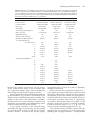
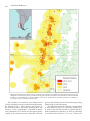
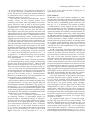
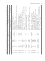
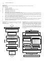
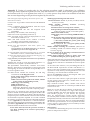
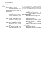
Notornis, 2007, Vol. 54: 121-136
0029-4470 © The Ornithological Society of New Zealand, Inc.
121
Validating locations from CLS:Argos satellite telemetry
D.G. NICHOLLS
31 Northcote Road, Armadale, Victoria 3143, Australia
C.J.R.ROBERTSON*
P.O. Box 12397, Wellington 6144, New Zealand
[email protected]
Abstract Satellite tracking, with the CLS:Argos system, has provided enormous benefits to wildlife studies, especially
for oceanic bird species. The system provides 2 locations, (1 from each side of the satellite orbit), but they are irregular
over time and of variable accuracy. Procedures are described here to identify outlier locations and retain the maximum
number of valid observations from DIAG files, thus producing a more homogeneous data set from which to map
distributions, track movements, and investigate behaviour, while determining the rate and direction of travel.
Nicholls, D.G; Robertson, C.J.R. 2007. Validating locations from CLS:Argos satellite telemetry. Notornis 54(3): 121-136.
Keywords Argos; telemetry; animal tracking; oceanic birds; flight speed; albatross;shearwater; bird distribution
INTRODUCTION
Satellite tracking, using the CLS:Argos system, has
provided enormous benefits to wildlife studies,
especially for oceanic bird species. The system links
a location and data collection receiver aboard NOAA
satellites and miniature low-powered transmitters
(platform transmitter terminals [PTT]) attached
to wild animals. It uses the Doppler effect, i.e. the
change of a PTT’s radio frequency, to determine
the location. The satellites are in polar orbit, each
passing overhead every c.3 h, and up to 4 satellites
are available to locate any PTT-tagged animal. The
satellite orbits are not equally spaced relative to
each another and so the resulting locations are not
spaced regularly throughout the day. The frequency
of reported locations is highest at high latitudes and
decreases with latitudes approaching the Equator.
Up to 20 location records, of variable positional
accuracy (Anon. 1999; CLS:Argos FAQ) day-1 can
be obtained from a tracked animal. The challenge
for the researcher is to retain the maximum number
of observations, after using explicit and objective
criteria to eliminate outliers points, to produce
a homogeneous data set from which to map the
animal’s distribution, trace movements or investigate
behaviour, and to determine the rate of travel.
CLS:Argos grades the location records according
to 3 criteria, according to the CLS:Argos (Argos)
assessment of the animal being tracked (e.g.,
Received 2 Aug 2006; accepted 31 March 2007
*Corresponding author
speed of movement) (Anon. 1999): (a) Location
Class (LC) indicates accuracy (LC =3, 2, 1 have an
accuracy of <1 km, LC =0 > 1 km, and A, B, Z each
have an unspecified accuracy; (b) Quality Index
(IQ) has 2 components, based on frequency and
signal stability, number and timing of the received
signals, that summarise the variables affecting the
Argos location calculation (highest values indicate
better transmitter performance); (c) Plausibility
Tests Passed (NOPC) grades the reliability of the
record using tests for residual error, transmission
frequency continuity, movement of the transmitter,
and plausible velocity from previous position
(Anon. 1999)(4 tests passed best, <2 invalid).
The CLS:Argos system, provides a variety of
data file formats and, if requested, can include the
provision of “Location Service Plus”. This auxiliary
service provides all of their determinations of
location, not just those validated locations of high
quality that are normally provided (COM or PRV
files). This Location Service Plus facility is essential
for researchers using low power PTTs, depending
on the economics and requirements of their study.
For each location determination by the system,
there are 2 possible solutions, 1 on each side of the
ground track of a satellite’s orbit (CLS:Argos FAQ).
The user of a DIAG or PRV/C file is responsible for
selecting the correct solution from these 2 location
sets. The locations provided differ significantly
in their accuracy, depending on the quality of the
transmission and its reception. The Argos definition
of the accuracy for the position ranges from “<1 km”
122
Nicholls & Robertson
to “indeterminate and unspecified”. The system
provides diagnostic information (e.g., IQ) to help
researchers interpret the accuracy of each location
determination.
The solutions developed by previous workers
that are used presently by researchers to extract as
much valid location data as possible include using
only locations of known accuracy (e.g., LC =3, 2, 1)
to establish the locations used to map the routes
taken by albatrosses (Diomedeiidae). Poorer class
records were clustered along the lines demonstrated
by the “quality” records (Weimerskirch et al. 1992).
Filtering procedures were perfected for slowermoving species, using a single maximum speed of
travel, 1st for seals (McConnell et al. 1992), and later
other speeds were used for studies on penguin and
albatross (Brothers et al. 1998). Klomp & Schultz
(1998) used 2 different speed thresholds for the short
and long time intervals between successive locations
to select points for their studies of shearwaters.
Other workers (Anderson et al. 1998) have
arbitrarily discarded the poorest accuracy Locality
Classes (e.g., Z). An alternative method (Nicholls et
al. 1994) used a running average of 3 points weighted
for the LC and the current and adjacent locations,
later allowing for the difference in time between the
3 locations (Freeman et al. 1997). This method used
all the locations provided and generated a possible
flight path smoothed between the location points.
As our pelagic seabird-tracking and validation
experiments (1992-2001) proceeded, we progressively
lengthened the intended duration of deployments
(up to >2 years for some deployments), and the
transmitters were operated intermittently with duty
cycles of 3-23 h “on” and 3-160 h “off” to prolong
battery life. Each transmitter had a pulsed signal,
with a repetition rate of 60-90 s, that operated during
the “on”-periods.
The error of individual locations has been
measured for stationary transmitters (Weimerskirch
et al. 1992; Anderson et al. 1998; Brothers et al. 1998;
Nicholls et al. 2007), but it was previously suggested
to be 10 km for birds at sea (Prince et al. 1992). More
recently, the development of improved satellite
receivers, smaller PTTs, revised and additional
(since mid-1994) LCs (0, A, B, Z) with a new method
of calculating the location by CLS:Argos (Anon.
1994) have all improved the quality of positions
obtained from Argos. The accuracy of locations
have also been measured for moving transmitters
on small ships, a car circling a proving circuit at
variable speeds, and on a transcontinental train
(Nicholls et al. 2007)
Between 1998 and 2001, we analysed albatross
and shearwater flight data using DIAG files
collected from latitudes between the Equator and
the Antarctic using various PTTs, over a wide range
of transmitting regimes, and with 2-4 satellites
determining locations, a combination of factors
not generally applied in tracking programs. We
considered it was desirable to judge each location
in its context rather than to apply an automated
filter (originally designed for seals, McConnell et al.
1992), or to use a small set of fixed criteria. Although
time-consuming during the development of the
technique, the individual assessment procedure
resulted in the retention of a higher proportion
of the observations and a better understanding of
the quality of the data, and of other behavioural
implications (Nicholls et al. 2005).
Data preparation
CLS:Argos provides a record with a pair of
locations and diagnostic information about their
determination in the DIAG file (Appendix A). The
record is obtained from either real-time downloads
using the DIAG command, or the equivalent DIAG
archival file which contains the complete dataset,
supplied by CLS:Argos. This file typically has
a 6-line record for each location determination
(Appendix A). The fields include PTT number,
date, LC, and IQ in the 1st line and the 2 alternate
locations on the next line. Other diagnostic data
follow in the next 3 lines, with the measurements
from the PTT sensors or extra messages in the last
line or lines. The complete record is described in the
CLS:Argos manual (Anon. 1999).
In this DIAG format, researchers can read location
records easily, but these need to be converted into a
spreadsheet or database format to aid sorting, and
to assess, select, and map the useable locations.
Concatenating the 6-line archival data into a 1-line
record is achieved by stripping the field names, units,
and extra carriage returns from the multi-line record.
A word processor or editor allows the global selection
and replacement of the field names (e.g., “Date :”,
“Lat 1 :”) with a tab, and the carriage return between
lines, by replacing the carriage return and the 1st
field name of the next line with a tab. This process
can , of course, be automated by use of a macro (not
described here). Others have written customised
programs (McConnell et al. 1992; Brothers et al. 1998).
We then stored the data in a Excel® database, arranged
to calculate some fields (Julian day, numeric decimal
versions of LAT1, LON1, LAT2, LON2): and these
calculation formulae have not been included in the
procedures described here.
Preparing the records (Appendix B) for selection
(a) Each record is labelled with a unique serial
number.
(b) Locations from text fields of geographic
coordinates (e.g., 30.5°N or 55°S) must be
converted into numeric values where the
northern and southern latitudes are respectively
positive and negative (30.5, -55.0, respectively)
and eastern and western longitudes (e.g., 170°E
Validating satellite locations
or 175°W) respectively changed to positive
and negative numeric values (170.0, -175.0,
respectively). The latitudes and longitudes
for each of the 2 possible Argos locations are
converted into numbers and a copy made of
the 1st nominated location (Appendix B).
(c) Calculate the ‘Julian day’ from DateTime.
(d) Mark and remove the pre- and post-deployment
records to the bottom of the sheet.
(e) Records without a location (LC = Z, latitude =
????? and longitude = ??????) are excluded by
sorting and moving them to the bottom of the
spreadsheet.
(f) A numeric field, ‘Reason’, with the value of 1
is added to all records indicating that the 1st
location is selected. The time interval, distance,
and speed from the previous to the present
position are calculated using great circle
distance (Appendix B).
(g) A calculated field, ‘Flag’, detects records that
need visual checking because the speed is too
high, or, the time interval between records is
very short.
(h) Further descriptive character fields for the
identification of the animal (Species, Location,
Sex, Band Number, Name) are added according
to need. See Appendix B for the file specification
and spreadsheet formulae used for the various
calculations.
These steps may be achieved within a database
where the records can also be identified by a unique
number, stored, sorted, and selections exported (e.g.,
Prince et al. 1992). We imported a tab-delimited text
file into a database, calculated some fields and then
exported into a pre-constructed Microsoft® Excel®
template spreadsheet. The formulae of the calculated
fields within the spreadsheet are applied to the entire
file, except for the no-location records (“Z???????”)
and pre- and post-deployment records. All criteria
for the selection can be displayed in consecutive
columns to facilitate visual comparison.
Originally, we developed an entirely visual
selection process, but subsequently developed
the automatic flagging procedures shown in
Appendices B-F and in Table 1. In this process each
record is considered in relation to the locations
immediately before and after that record.
When determining if a record is valid, we consider
LC, IQ, time interval between locations, speed (and
its rate of change), along with the trends before and
after in latitude and longitude. We experimented by
excluding suspect locations and then comparing the
changes in the time intervals, distances, and speeds
that were recalculated when changes are made in the
‘Reason’ field. The results of any change could be
seen immediately in the revised distances, times, and
speeds (Appendix B). The ‘Reason’ for the change
is recorded (e.g., if the 2nd location was the more
123
likely correct location, or, the record was improbable
because of poor LC and IQ) using the classification
scheme and guides in Appendices C-F. After the 1st
pass through the file, marked records are excluded
(other than those where the 2nd locations were used
– ‘Reason’ 2) and the process is repeated for any
flagged records that remain.
Others have independently measured or used the
occurrence of similar speeds to determine arbitrary
selection (Weimerskirch et al. 1992; Brothers et al.
1998). After inspecting the frequency distribution of
our calculated point-to-point speeds, we explored
different maximum speed thresholds of 40-120 km
h-1, and eventually selected 60 km h-1 as the warning
‘flag’ threshold for 3 species of Diomedea and 50 km
h-1 for 1 Thalassarche albatross). Setting the threshold
too high can include probable outlying points in
the final data set; setting it too low can result in too
many flagged points having to be considered and
valid locations being wrongly excluded.
Selection
To aid inconsistently finding possible outliers (see
Appendices B-F; Table 1), each record is automatically
flagged if the speed exceeds a predetermined value,
such as 60 km h-1 for northern royal albatross Diomedea
sanfordi, 50 km h-1 for Chatham albatross (Thalassarche
eremita) and 40 km h-1 for sooty shearwater (Puffinus
griseus), or, the time since the previous record is < 0.3
h. The speeds and time are chosen as a warning; they
are not in themselves sufficient reason for marking a
record for exclusion.
Each flagged observation is first checked to
determine if the alternate location is the more likely
location position. Excessive speed (e.g., >200 km
h-1) and a “large” distance, immediately followed
by a record with a similar distance, are clues that
the alternate location may be preferable: Location
2 is then substituted as the selected location and
time, the ‘Reason’ is marked as “2”, and a revised
distance and speed are automatically recalculated.
Where the transmitters are operated continuously,
the correct location is almost invariably selected
by CLS:Argos, but as the “off” period in the
transmission regime lengthens, alternate locations
are increasingly likely.
With 3, and sometimes 4, satellites available,
there are a few occasions when the consecutive
locations are simultaneous (exceptionally), or only
seconds apart. Over such short time periods any
error in the location creates impossibly high speeds.
We selected 0.3 h (18 min) as the time interval to
warn for this condition.
Stepping through the Excel® file, each “present”
record being considered is compared with the
previous selected record. Initially all records are
selected, but as records resulting in excessive speed
or distance are excluded, each comparison is made
-44.455
-44.377
-44.800
-44.631
-44.423
-44.433
-44.473
-44.479
-44.437
-44.435
-44.435
-175.963
-176.341
-176.042
-176.222
-176.242
-176.260
-176.839
-176.232
-176.247
-176.222
1
1
1
5
1
1
1
1
5
5
1
3
1
-44.652
1
1
-176.134
-44.434
-176.237
-176.060
-44.364
-176.278
5
-44.692
-44.243
-175.795
1
1
-176.035
-44.436
-176.236
4
-44.437
-176.239
1
1
-44.444
-176.280
1
1
-45.120
-44.438
-176.245
-44.684
-44.433
-176.223
1
-176.037
-44.426
-176.248
Reason
-176.632
Lat
Long
2
1
48
46
5
2
27
30
56
16
23
5
1
67
82
8
41
41
0
3
3
2
2
2
Distance
0.8
22.6
3
0
74
47
1
18
2
18
262
3
-
14
101
1
41
4
5
20
503
0
2
11
3
3
2
Speed
0.6
0.3
0.9
1.5
0.1
22
0.0
1.6
0.0
1.7
1.7
22.2
1.7
2.1
0.1
23.8
1.4
0.3
0.6
0.8
0.8
Time
Too fast
Too soon
Too soon
Too soon
Too soon
Too soon
Too soon
Flag
1-56
1-50
2-56
B-00
0-56
1-57
1-55
0-50
B-00
B-00
0-48
0-56
1-57
1-50
A-05
1-50
B-00
B-00
0-57
1-58
0-48
1-58
B-00
2-58
LC-IQ
-176.22
-176.25
-176.23
-176.26
-176.24
-176.22
-176.04
-176.13
-176.04
-176.04
-176.24
-176.28
-176.24
-176.24
-176.28
-176.25
-176.22
-176.25
-44.44
-44.44
-44.44
-44.47
-44.43
-44.42
-44.63
-44.46
-44.69
-44.68
-44.43
-44.36
-44.44
-44.44
-44.44
-44.44
-44.43
-44.43
Selected positions
2
1
5
Excluded, fast in context
and poor quality, long spike
5
2
27
21*
1
Excluded, too fast; 2
satellites
27
Excluded simultaneous
record, poor quality
Excluded, see next record
8
Excluded; no flag but Lat
spike; poor LC-IQ
32
0
Excluded, note Long spike
with next distance
9
3
3
2
2
2
Revised distance
0.8
22.6
1.6
0.3
0.9
1.5
22.1
1.7
1.7
23.8
1.7
2.2
23.8
1.4
0.3
0.6
0.8
0.8
Time interval
3
0
3
18
2
18
16
1
1
5
4
0
2
11
3
3
2
Speed
Table 1 Annotated selection of PTT location records to indicate the selection process described in the text; see also Fig. 2 for mapped results. Data from Chatham
albatross (Thalassarche eremita) deployment PTT #2222 11 Nov 1998 - 15 Nov 1998. *Retained cf. Prior record. Long, longitude; lat, latitude; distances in km; time in h;
speed in km h-1 ; positions in longitude then latitude.
124
Validating satellite locations
125
Table 2 Examples of satellite tracking locations comparing the quality of records received from
the CLS:Argos system for different species, for different PTT duty cycles, and different repetition
rates of transmissions. Records accepted/rejected; records accepted or rejected during selection
process during selection process; Percentage distribution; percentage distribution for number of
messages received (satellite pass)-1 for each PTT.
Diomedea sanfordi
23738-2
PTT ID deployment-1
Location start
43.598S 176.861W
Location finish
34.751S 113.846E
Date start
28 Jan 1997
Date finish
15 Aug 1998
Active deployment (days)
564
Duty cycle (h)
9 on/135 off
Repetition rate (s)
90
Total records received
577
Records accepted/rejected
461/116
% accepted/rejected
Location class 3
0.7/2
5.0/1
16.3/0.2
0
45.4/3.6
A
5.7/2.1
B
5.0/1.6
Z
1.6/1.4
Z???
-/11.3
Percentage distribution
12
11
10
0.5/9
3.8/0.2
8
8.8/1.0
7
14.2/1.6
6
13.3/1.9
5
13.7/1.4
4
14.6/1.2
3
5.9/2.6
2
5.0/1.9
1
-/8.3
between the present and the last selected record.
If this earlier record needs to be excluded, then
the comparison begins again after including the
intervening, but previously excluded, records.
Speeds greater than the predetermined mark set
by the researcher (e.g., 60 km h-1 for northern royal
albatross) are considered particularly carefully. The
quality of the record, the speed before and after,
and the trend in the rate of change of latitude and
longitude, are considered when determining which
of the 2 locations has the poorer quality.
If the speeds adjacent to the interval being
considered are high, or increasing, and the quality
(LC and IQ) of the records is good, the records are
retained. Where 1 or other of the poorer quality
Thalassarche eremita
23081
44.453S 176.315W
6.396S 81.323W
17 Feb 1997
7 Jun 1997
110
3 on/ 3 off
77
480
404/76
Puffinus griseus
6750-4
45.534E 171.010E
42.930S 179.114E
13 Oct 1999
29 Oct 1999
16
Continuous
85
189
103/86
1.0/4.0/0.2
17.9/41.9/1.7
9.8/0.6
8.3/1.5
1.3/1.3
-/10.6
0.2/1.7/4.4/7.3/9.4/0.8
9.2/0.6
10.4/0.6
10.2/0.4
12.9/0.6
10.2/1.9
8.3/1.5
-/9.4
1.9/- 1.9/- 8.5/- 27.0/5.3
13.2/5.3
18.0/9.0
-/25.9
3.7/0.5
7.9/0.5
11.6/2.1
14.3/3.2
7.9/5.8
9.0/10.6
-/22.7
locations has an LC of A, B, or Z, then 1 is generally
marked for exclusion.
When 2 records for comparison both have LC =
0, the speeds to nearby locations are considered and
the quality indices (IQ) compared. If the speeds of
the adjacent records are similar, the high speed is
accepted and both locations are retained. However,
if the speed is greater than 40 km h-1 (depending
on species), and greater than twice either of the
previous, or the next, records, 1 is usually excluded.
If both records are poor, i.e. LC = A, B, or Z, the
poorer record is excluded (Appendices D – F).
The selected dataset locations should then be
mapped and any locations over land (other than
breeding sites of pelagic seabirds) — an improbable
126
Nicholls & Robertson
Fig. 2 Mapped results of removing Argos location points
selected using the process set out in the text (see data in
Table 1).
Fig. 1 Timelines of unselected flight speeds (A), comparing
the effects of arbitrary removal of the poorest Location
Classes (LC =0, A, B, Z) (B), and the selection of records
using the process set out in the text (C).
location for an albatross after it had left the breeding
location — rechecked.
A flow chart, an example, and a decision table
of the entire procedure are provided in Appendices
D-F and Table 1.
We used the deployment on a Chatham albatross,
that foraged at 2 locations and migrated across an ocean,
to illustrate a comparison between the 2 procedures
((a) progressive arbitrary removal of the poorest LC
of locations; (b) our visual selection procedure) for
detecting out-lying points in seabird flights determined
from CLS:Argos location files. The characteristics of the
dataset used are shown in Table 2, which shows the
initial removal of the “no location” (LC = Z???) records
before the selection processes began.
(a) We excluded 1 LC at a time beginning, with
the least accurate LC =Z progressing through
to LC =3, 2 & 1. Initially, with the full dataset
(Fig. 1A), there were speeds of >200 km h-1, but
as the arbitrary LC locations were removed,
the number of excessive speeds declined until
there were none >50 km h-1. At this stage only
26% of the original dataset (only records with
LC =3, 2, 1; Fig. 1B) remained.).
(b) We applied the visual selection procedure
described here to the same dataset and plotted
the resulting speeds (Fig. 1C). This process
retained 94.2% of the original dataset and the
maximum speed was reduced to 85 km h-1.
RESULTS
The 2 procedures yielded broadly similar flight
patterns. The speeds waxed and waned over the
deployment, with bursts of high speeds sustained
over several days as the bird migrated across the
southern Pacific Ocean (Nicholls & Robertson 2007).
However, arbitrarily and progressively excluding
locations with LC values of Z, B, A, and 0 ultimately
removed some 74% of the records, whereas the
visual procedure excluded 5.8% from the same
dataset. It is important to note that the range of
speeds is significantly higher for the visual selection
process. As speed is a factor of time interval, the
fewer records from the arbitrary selection obviously
ensure the resultant artefact of lower speeds.
The quality of the records received from
CLS:Argos over deployments for 3 species with
Validating satellite locations
127
Fig. 3 Demonstration of selected and excluded Argos locations of a northern royal albatross (Diomedea
sanfordi) moving along the coast of Chile achieved using selection procedure set out in the text.
PTTs of differing duty cycles and repetition rates
are compared in Table 2. The most notable feature
is the poorer quality of the material received from
the sooty shearwater (Nicholls et al. 2007). However,
an explanation may be that the shearwater often
dives and it has a less stable flight pattern in
comparison to that of the larger albatrosses, both
of which would make receipt of its transmissions
more difficult.
Table 1 and Fig. 2 illustrate an example of
our selection process applied to the tabulated
spreadsheet information; reasons for exclusions are
shown. The original and selected data are mapped in
Fig. 2 to show the results of the selection process.
128
Nicholls & Robertson
Fig. 4 Demonstration of selected Argos locations of a northern royal albatross (Diomedea sanfordi) moving
along the coast of Chile (see Fig. 3) achieved using the selection procedure set out in the text. Each selected
location is surrounded by a circular buffer (see text) to represent the possible precision according to
Location Class (LC) of that location point.
The locations of a northern royal albatross off
Chile in comparison to the coastline and bathymetry
are plotted in Fig. 3. This species is not known to
fly over land after it leaves the breeding area. All
except 1 of the “improbable” over-land locations
were identified for exclusion by the speed-quality
criteria of the selection process. After the selection
process, the refined at-sea locations showed a strong
relationship to the bathymetry.
The selected records shown in Fig. 3 are examined
in more detail in Fig. 4, in which the quality (LC)
of each of the selected records is surrounded by a
buffer (defined by Nicholls et al. 2007) at a distance
of <2.5 km for records of LC = 3, 2, or 1, 15 km for LC
Validating satellite locations
= A, and 25 km for LC = 0. Location records with LC
= B, Z were allocated an arbitrary error distance of
56 km. The levels of quality give another indication
of information lost if various classes of record are
arbitrarily removed, as in Fig. 1.
The selection processes identified the poorer
Locality Classes as the location points most
commonly associated with improbable or excessive
speed. However, some of each of the poor-quality
LCs need not be excluded, even for the poorest LC.
Locations of LC = Z, B, and A are often single points
deviating only a short distance from the trend of
direct flights, and if this poor quality coincided with
a long time interval, a normal flight speed resulted.
This situation existed for LC = 0 observations as well,
although less frequently. Where a high-speed was
flagged, and the consecutive locations were both LC
= 0 with IQ values of both records equalling 40, 44,
46 (and less often 48), either of the pair of records
was often plausible and the choice was consequently
difficult. It was generally determined on the trend
of latitude and longitude, selecting for the smoother
flight direction and speed, or arbitrarily excluding
the 2nd of the 2 equal-quality locations. Nicholls
et al. (2007) note the different precision of LC = A
as against LC = 0. Researchers may need to modify
their selection process accordingly, to reflect their
own requirements.
As a result of this visual selection procedure,
the calculated (point to point) speeds of remaining
records were all less than 100 km h-1. There are still
many records with speeds over 50 km h-1 (Fig. 1C).
These records would have been excluded if only LC
= 3, 2, or 1 were used. We considered them to be valid
observations because, with many records (especially
on fast migrations), the distances travelled are so
great that the location error is inconsequential.
Moreover, for birds that fly very long distances, the
high speeds can be sustained for days.
Speeds determined from records of LC = 3, 2 , and
1 only produced biases in the sample resulting from
over-representation of long time periods between
the infrequent retained observations. The paucity of
records of LC = 3, 2, or 1 was exacerbated when long
or intermittent duty-cycle transmission regimes were
used to study migration (when faster sustained speeds
were observed). For example, few useable data would
remain for the sooty shearwater (Table 2).
The data give a consistent impression that
an increased number of improbable points are
observed after a substantial change of direction,
at the 1st point of a long flight after local foraging,
and with the 1st location point after a long period
of no transmissions (Nicholls et al. 2007). A mixture
of locations of LC = 0, IQ =40-46, and an occasional
LC = 1 location, may indicate that a bird was resting
on the sea, or proceeding in a series of slow local
flights. Likewise, a set of locations of LC = 0, A,
129
B, or Z may occur when the bird is flying fast, or
quartering a local area.
DISCUSSION
Researchers have used various methods to select
records from CLS:Argos datasets. Of these methods,
progressively removing the poorest Locality Classes
did not remove improbable points until only the
best (LC =3, 2, 1) remained. The residue is usually
a small minority of the original records. The time
intervals between the few remaining locations are
thus usually relatively long, and the resultant flying
speeds are biased and certainly under-estimated. As
changes in the flight speeds vary widely depending
on the time interval, a single or limited number of
threshold speeds for determining improbable speeds
are also insensitive criteria. Simple exclusion rules
(setting aside the poorest locations, or filtering based
on a single speed threshold) have the advantage
of simplicity and reduced processing time, but we
consider the loss and simplification of the original
data to be too severe.
In the processing procedure reported here, it
should be emphasised that, although records are
removed, the time intervals, distances, and speeds
are recalculated within the revised set of records.
The sum of the time intervals between records
therefore equals the time between the 1st and last
records. The sum of the distances is progressively
reduced as the number of records is reduced and the
exceptional speeds are eliminated. A chain of records
is maintained and removing poorer combinations
provides slightly different representations of the
flight, progressively straightening the representation
of the flight, as more and more records are not used.
The final representation should meet the criterion
that there are no biologically impossible points.
Our close inspection of the pattern of locations
indicated that the poorer quality records of LC =
0, A, B, and Z generally result from poor satellite
reception. However, there are other instances where
the reception was good (strong signal strength,
many messages), but the signal was unstable. One
interpretation is that a series of poor locations
result when a bird flies fast with many changes in
direction, e.g., when it is foraging over a small area.
Such flights could affect the Doppler shift measured
by the CLS:Argos receiver and the resulting location
would be calculated incorrectly (CLS:Argos FAQ;
Nicholls et al. 2007).
An apparent flight path of 20-100 km pointto-point zig-zags must not be taken literally. The
location measurements are made during the 3-16
min of a satellite pass during which an albatross
could indeed have turned 180°, or it could have
flown more than 10-20 km, a distance considerably
greater than the specified accuracy of LC = 3, 2, or 1.
If these flights also include a landing on the sea and
130
Nicholls & Robertson
submergence, with associated temperature shocks
to the transmitter, it would cause an unstable signal
that would distort the Doppler calculation.
Inspection of the full diagnostic information
(DIAG file) provided from CLS:Argos during the
consideration of the calculated distance and speed
produced a homogeneous set of locations. There
were no excessive speeds between successive
locations. The visual selection procedure described
here retained a higher proportion of locations
than other procedures already described, without
compromising the validity of the tracking.
The selection procedure we have applied to CLS :
Argos location data has been tested against tracking
studies for 2 genera of albatrosses and 2 shearwaters
(Puffinus spp.). The consistent identification and
exclusion of improbable locations helps in relating a
bird’s position and movements to atmospheric and
oceanographic features. We believe the procedure
may assist other researchers in improving the use of
their satellite tracking data for similar studies.
ACKNOWLEDGEMENTS
Satellite tracking experiments producing the data for
developing this technique were funded by the New
Zealand Department of Conservation, the Australian
Research Council, the Ian Potter Foundation, the World
Wide Fund for Nature (Australia), Environment Australia,
the W. V. Scott Estate, and private donors. La Trobe
University supported many of these tracking studies for
more than 20 years. G.P. Elliott and M. Harger provided
assistance with the great circle calculations. M.D. Murray
provided critical advice throughout the study. Southlight
farm and S. McGrouther generously provided the facility
and accommodation on the Otago Peninsula where much
of the process was refined over 3 summers (1998-2001).
Chisholm Institute has generously supported the salary
of D.G. Nicholls, while C.J.R. Robertson was employed
by the New Zealand Department of Conservation until
May 2000, and by Wild Press subsequently. Without the
support and encouragement of these organisations this
work would not have been completed.
LITERATURE CITED
Anon. 1994. CLS : New Argos location. News Flash. CLS,
Toulouse, France, July 1994.
Anon. 1999. The Argos user’s manual. Maryland, USA,
Argos CLS, Landover.
Anderson, D.J.; Schwandt, A.J.; Douglas, H. 1998. Foraging
ranges of waved albatrosses in the eastern tropical
Pacific Ocean. pp. 180-185 In: Robertson, G.; Gales,
R. (ed.) Albatross biology and conservation, Chipping
Norton, Australia, Surrey Beatty & Sons.
Brothers, N.; Gales, R.; Hedd, A.; Robertson, G. 1998.
Foraging movements of the shy albatross Diomedea
cauta breeding in Australia: implications for interaction
with longline fisheries. Ibis 140: 446-457.
CLS:Argos FAQ .http://ftp.cls.fr/html/argos/general/faq_
fr.html
Freeman, A.N.D.; Nicholls, D.G.; Wilson, K.-J.; Bartle, J. A.
1997. Radio- and satellite-tracking Westland petrels
Procellaria westlandica. Marine ornithology 25: 31-36.
Klomp, N.I.; Schultz, M.A. 1998. The remarkable foraging
behaviour of short-tailed shearwaters breeding in
eastern Australia. Ostrich 69: 373.
McConnell, B.J.; Chambers, C.; Fedak, M.A. 1992. Foraging
ecology of southern elephant seals in relation to the
bathymetry and productivity of the Southern Ocean.
Antarctic science 4: 393-398.
Nicholls, D.G.; Murray, M.D.; Robertson, C.J.R. 1994.
Oceanic flights of the northern royal albatross
Diomedea epomophora sanfordi using satellite telemetry.
Corella 18: 50-52.
Nicholls, D.G.; Robertson, C.J.R. 2007. Assessing flight
characteristics of the Chatham albatross Thalassarche
eremita from satellite tracking. Notornis 54: 168-179.
Nicholls, D.G.; Robertson, C.J.R.; Naef-Daenzer, B. 2005.
Evaluating distribution modelling using kernel
functions for northern royal albatrosses off South
America. Notornis 52: 223-235.
Nicholls, D.G.; Robertson, C.J.R.; Murray, M.D. 2007.
Measuring accuracy and precision for CLS:Argos
satellite telemetry locations. Notornis 54: 137-157.
Prince, P.A.; Wood, A.G.; Barton, T.; Croxall, J.P. 1992.
Satellite tracking of wandering albatrosses (Diomedea
exulans) in the South Atlantic. Antarctic science 4:
31-36.
Weimerskirch, H. 1998. Foraging strategies of Indian
Ocean albatrosses and their relationship with fisheries.
pp. 168-179 In: Robertson, G.; Gales, R. (ed.) Albatross
biology and conservation. Chipping Norton, Australia,
Surrey Beatty & Sons Pty.
Weimerskirch, H.; Salamolard, M.; Jouventin, P. 1992.
Satellite telemetry of foraging movements in the
wandering albatross. pp. 185-198 In: Priede, I.G.;
Swift, S.M. (ed.) Wildlife telemetry: remote monitoring
and tracking of animals. Chichester, United Kingdom,
Ellis Horwood.
Appendix A Typical CLS:Argos DIAG file record.
Program 0137
02222 Date : 02.01.99 00:39:45
LC: 1 IQ : 50
Lat1 : 42.762S Lon1 : 164.245W Lat2 : 31.473S lon2 : 110.717W
Nb mes : 008
Nb mes>-120dB : 0 Best level : -124 dB
Pass Duration : 255s
NOPC : 2
Calcul freq : 401 6650276.4 Hz Altitude : 000 m
12
255
136
45
Field Name
Type
Typical value
YES
YES
YES
YES
YES
YES
YES
YES
YES
YES
YES
YES
YES
YES
YES
YES
YES
YES
S
S
F
G
H
I
J
K
L
M
N
O
P
Q
R
S
T
U
Record ID #
Julian Day
Frequency
d1
d2
d3
d4
Pass Duration
NOPC
Best signal
strength
LAT1
LON1
LAT2
LON2
# messages
# strong
line #
PTT #
Date
LC
IQ
integer
4 DP number
1 DP number
integer
integer
integer
integer
integer
integer
integer
text
text
text
text
integer
integer
integer
integer
18 ch text
text
text
991347
39.2629
401653041.8
25
4
1
255
77
2
-128
45.792S
170.746E
42.099S
170.019W
4
0
21
23081
08.02.99 06:18:36
0
46
* YES = data from Argos DIAG File. S = essential for selection process.
*
A
B
C
D
E
Col
DP = decimal place(s)
Unique identification number supplied by user.
Number of days (and decimal fraction of day) counting from day 1 as 1
January of the year. Formula not supplied. User must calculate from Date
field in spreadsheet or external database.
Argos calculated radio frequency of the PTT in MHz.
Next four fields report the measurement from sensors.
Sensors and data are variously configured and formatted.
See Argos Users Centre and PTT manufacture.
Usually four 8-bit numbers, i.e. four numbers 0-255 measuring, eg.
temperature, battery voltage, activity and others.
Time between first and last messages in seconds.
Number of plausibility tests passed. A guide to reliability of record. Range
1-4.
Signal strength of the strongest signal in the pass, units dB; typical range
from bird PTTs is -128 (strong) to -133(weak).
Latitude of the first position calculated by Argos.
Longitude of the first position calculated by Argos.
Latitude of the second position calculated by Argos.
Longitude of the second position calculated by Argos.
Number of messages received by Argos in the pass; range 1-~16.
Number of messages received by Argos with a signal strength greater than
-120 dB.
Optional field to aid sorting, referring to records.
Unique identification of PTT supplied by CLS : Argos.
Date : DD.MM.YY HH:mm:ss.
Location class, values 3, 2, 1, 0, A, B, or Z.
Two code numbers describing PTT performance within and between satellite
passes respectively
H = generally hidden during selection.
Description and explanation - Formula
Appendix B File and column specifications for an Excel® spreadsheet used for the procedure for selection of records explained in text.
Validating satellite locations
131
S
S
S
S
S
S
SH
S
H
H
H
H
H
H
V
W
X
Y
Z
AA
AB
AC
AD
AE
AF
AG
AH
AI
Spp / Loc
Sex
Name
Speed
Time Interval
Distance
REASON
lat. copy
lon.
lat.
LON2#
LAT2#
LON1#
LAT1#
Appendix B Continued.
4 ch text
1 ch text
8 ch text
0 DP
number
1 DP
number
0 DP
number
integer
3 DP number
3 DP number
3 DP number
3 DP number
3 DP number
3 DP number
3 DP number
CMPy
M
MrsCC
1
0.8
1
1
-45.792
170.746
-45.792
-170.019
-42.099
170.746
-45.792
Time in hours between previous and present record. Manually
insert 0 for first location of new deployment, or new PTT. Formula:
=(U4-U3)*24.
Speed in kph from the previous location to the present location.
Formula: =Distance/Time Interval, i.e. =AD4/(U4-U3)/24. Manually
insert 0 for first location of a new deployment, or a new PTT.
Four letter code for the species and the location of deployment start.
Code for sex.
Alias or nickname for animal and / or deployment.
Initially 1, changed to a value between 2 and 9 if location 2
is chosen or the record excluded. See Codes, Appendix C.
Formula: =1.
Great circle distance in km from previous location to the present.
Formula: =6366.0648*ACOS(SIN(Z4*PI()/180)*SIN(Z3*PI()/180)+
COS((AA4-AA3)*PI()/180)*COS(Z4*PI()/180)*COS(Z3*PI()/180)).
Manually insert 0 for first location of new deployment, new PTT.
Col. AB=Col. Z. This and the previous field (AA) used together in an X-Y
Excel chart to map the locations. Formula: =Z4.
Copy of LON1# initially. May be changed during selection process if LON2#
is the preferred. Formula: =W4.
Copy of LAT1# initially. May be changed during selection process if LAT2# is
preferred. Formula: =V4
LON2 as a decimal number. Formula not supplied. User must calculate from
LON2 field.
LAT2 as a decimal number. Formula not supplied. User must calculate from
LAT2 field.
LON1 as a decimal number. Negative values in Western Hemisphere.
Formula not supplied User must calculate from LON1 field.
LAT1 as a decimal number. Negative values in Southern Hemisphere.
Formula not supplied. User must calculate from LAT1 field in spreadsheet or
external database.
132
Nicholls & Robertson
H
S
S
S
S
S
S
S
S
S
AJ
AK
AL
AM
AN
AO
AP
AQ
AR
AS
Comment
Revised
Speed
Revised Time
Interval
Revised
Distance
last lat
last lon
Month
LC-IQ
BandNo
Flag
Appendix B Continued.
text
0 DP
number
1 DP
number
0 DP
number
2 DP
number
2 DP
number
integer
4 ch text
8 ch text
10 ch text
1
0.8
1
-45.792
170.746
2
B-00
R12345
Calculated field, if an accepted record, the lon. is copied to
this field. If an excluded record (Reason >2), then last selected
lon. - the previous record of this field - is copied into this field.
Formula: =IF(AC4<3,AA4,AP3).
Calculated field, if an accepted record, the lat. is copied to this
field. If an excluded record (Reason >2), then last selected
lat. - the previous record of this field - is copied into this field.
Formula: =IF(AC4<3,Z4,AQ3).
Distance automatically recalculated from this and last
selected location, triggered by a change in the REASON
field. Calculated field. Formula = 6366.0648*ACOS
(SIN(AO4*PI()/180)*SIN(AO3*PI()/180)+COS((AP4AP3)*PI()/180)*COS(AO4*PI()/180)*COS(AO3*PI()/180))
Revised Time Interval automatically recalculated from cumulative
Time Intervals from the last selected location, triggered by a change
in the REASON field. Formula: =IF($AC3<3,AE4,AE4+AT3)
Revised speed automatically conditionally calculated or recalculated
from Rev. Distance and Rev. Time Interval for selected locations only.
Triggered by changes in REASON field. Excluded records are blank.
Formula: =IF($AC4<3,AS4/AT4,””)
Explanation for exceptional retention or rejection selections.
Band Number
Calculated field detecting short Time Intervals or excessive speed.
Formula: =IF(B4=B3,(IF(AE4<0.3,”Too Soon”,IF(AF4>40,”Too
Fast”,””))),”NewPTT”). The Speed threshold, here set at 40, is set
manually and copied down the rows.
Calculated field concatenating LC, “-” and IQ. Used
in the selection process and as a mapping label.
Formula: =Concatenate(D4,”-”,E4)
Calculated field extracting month from Date field. Formula:
=VALUE(MID(C4,4,2)). Used as a label in mapping or analysis.
Validating satellite locations
133
134
Nicholls & Robertson
Appendix C
Selection criteria codes for marking CLS:Argos records during procedure for selecting records.
Code
1
2
3
4
5
6
7
8
9
L
Reason
Location 1 selected
Location 2 selected
Improbable record of LCs 3, 2, 1, or 0.
Improbable record of LC=A.
Improbable record of LC=B.
Improbable record of LC=Z, location index ≥ 10.
Record in wrong hemisphere. Presumed to be a transmission-reception error in the PTT identification
or an illegal transmission of an unregistered PTT with the same identification. Typically there are
only 1 or 2 messages and the location may coincide with the location of a manufacturer. Not used for
species that normally travel in both hemispheres.
Pre- or post-deployment locations. Locations obtained before and after the target deployment.
Typically locations obtained during testing or preparation.
Records with no location determined by Argos. Generally LC=Z and quality index 0 or 1. Records
damaged in transmission or transcription. Typically appear in DIAG as strings of ????????????.
Records overland and rejected.
APPENDIX D
Appendix D Flow chart demonstrating the selection
procedures for validating CLS:Argos records
explained in text.
Convert ARGOS archival DIAG file into tab delimited text file
Sort by PTT, Date,
Add Unique ID. Exclude duplicates. Add line #
Add deployment details (bird ID, …).
Mark pre- & post deployment records
Appendix E Flow chart demonstrating the selectionexclusion decisions needed for validating CLS:Argos
DIAG locations demonstrated in this paper. Note that
Nicholls et al. (2007) have noted a greater precision
for locations with LC =A as against those with LC =
0, so the process may need to be modified to take this
APPENDIX
E precision required by
into account depending
on the
the selector.
For ALL records, but concentrating on the flagged records, …
For each record, confirm first location is the better of the two locations.
Sort by latitude.
Exclude Z ???????.
Resort by PTT, Date (or line #)
Calculate Distance, Time Interval and Speeds.
Set thresholds for Flags.
Detect Flagged records.
IF NOT,
Compare location with previous two and next two records and select a
location from each pair giving the shortest distances between records.
IF second is location selected, set Reason = 2.
Compare the present record with the previous-unexcluded record.
Is the Flag “Too fast”?
Is the Flag “Too soon”?
Using LC-IQ, location, Distance, Speed
and Flags, exclude poor records.
See APPENDIX E.
IF YES
IF speed reasonable in context *
THEN retain both records.
ELSE exclude poorer record **.
Continue selection until no
excessive speeds remain.
Check no excessive speeds remain by
plotting speed against time.
Is there uncharacteristic
Or excessive zigzagging in the
lat. And / Or lon.?
Is the LC = A, B, Z?
IF YES
Consider excluding poorer record **.
Review selection thresholds
Map records and investigate on-land and
any other improbable records.
MAP,
SUMMARISE,
and
ANALYSE
selected records.
IF YES (see note)
IF both records are LC > 0 retain both.
IF both records are
equal to or better than LC-IQ =0-44,
and speed < speed threshold
and Time Interval > 0.2 h
THEN retain both
ELSE exclude poorer of two records.
IF LC of poorer record 0-<44 or = A, B, Z
THEN exclude this record.
IF YES
Consider excluding poorer record **.
Set Reason (see APPENDIX C), for each excluded record.
Inspect recalculated Revised Time Interval, Distance and Speed.
IF a record, two or more records away from the present has now been excluded
THEN reset Reason(s) of intervening records and reconsider next record from last excluded.
Set Reason, for these excluded records.
Consider NEXT record UNTIL end of file.
* See pseudo code for a definition of excessive speed in Appendix F and text.
** See pseudo code for subroutine in Appendix F, to determine poorer record.
Validating satellite locations
135
Appendix F Listing of pseudo-code for the selection procedure (with 2 subroutines) for validating
CLS:Argos DIAG locations explained in textr. Note that Nicholls et al. (2007) have noted a greater precision
for locations with LC =A as against those with LC = 0, so the process may need to be modified to take this
into account depending on the precision required by the selector.
(The investigator, before beginning the selection process, sets
Instructions in italics)
Convert CLS : Argos DIAG archive file into tab-delimited
text file
Create a template Excel spreadsheet with the layout
according to Appendix B
Import tab-delimited file into the template Excel
spreadsheet
Sort data by PTT and date / time chronology
Label each record sequentially (with Line #)
Select and mark all pre- and post-deployments for each
PTT-animal, Set Reason = 8
Select and mark records ??????? without a location
(ascending sort by latitude, Set Reason = 9
Sort (ascending) retained records on field Line #
Identify each bird deployment with Name, Species, Sex,
...{Optional}
Copy formulae for all fields marked as “S” in Excel
spreadsheet for all records (Appendix B)
Set speed threshold in formula for warning flag (eg. suggested
Diomedea = 60 km h-1, Thalassarche = 40 km h-1)
Set short time interval value in formula for warning flag (eg.
suggested Time Interval = 0.3 h)
Copy formulae from template down the Excel spreadsheet
for all records
Initialise first record for each PTT-animal (Distance = 0,
Time Interval = 0, Speed = 0) and Set Reason = 1
The Spreadsheet automatically calculates and inserts
Distance, Time Interval, and Speed to each new point with
warning flags to mark records that are improbably fast or
too close together in time
For ALL records consider the locations, lat. and long
Concentrate on the flagged records
IF, the wrong mirror-image location lat. and lon. is
given by CLS : Argos
THEN select the better point from LAT2#, LON2#
in the context of surrounding records,
THEN copy to lat and long,
THEN set Reason = 2
ELSE proceed to next step
(Indication - distance for consecutive records is very
large and dissimilar compared to adjacent points)
This process of comparison of the present record with the
previous selected record continues throughout the file. If the
previous record is marked for exclusion, then the selectioncomparison process must backtrack to the last earlier selected
record and the comparison repeated. As a record is marked
for exclusion, a reason for the exclusion is allocated; set Reason
= 3 to 6 (Appendix C). If the Reason > 2 then the Distance,
Time Interval and Speed are automatically recalculated in the
spreadsheet (Appendix B). These revised figures are then also
used to determine if a better choice can be made.
IF the time interval from the previous location is
very short, resulting in an excessive speed, (Flag =
“Too Soon”),
THEN apply following tests and actions
IF both locations are LC =3, 2 or 1 (excellent, knownaccuracy records)
THEN consider retaining locations (assuming
reasonable speed)
IF both locations are LC-IQ =0-44 or better,
AND speed<speed-threshold, AND time > 0.2 h (i.e.
moderate quality records, reasonable speeds)
THEN retain both records,
ELSE mark poorer record using Subroutine A
below
IF the speed to the present point was excessive **
(see below) compared to adjacent points (Flag
= “Too Fast”) exclude the poorer point using
Subroutine B below
IF LC =A, B, or Z (i.e. a very poor quality record)
(see note in caption)
THEN consider marking for exclusion. (Reasons for
excluding include an isolated change in speed or
excessive zig-zag)
IF rate of change in lat and long is uncharacteristic or
excessively zig-zagging
THEN inspect adjacent records to detect cause and
consider marking the poorer quality record
At the end of the selection, plot speed of the selected records
against date / time. Confirm there are no improbable speed
records. Review selections or thresholds if excessive speeds
remain.
At the end of the selection, sort (Ascending) the file on
the Reason field. Separate the records with Reason > 2.
These are now the excluded records. In a spreadsheet this
separation is easily done by inserting blank new rows and
annotating a row ahead of the excluded records.
Re-sort the selected records in chronological order (use
line # as a simple quick solution).
At the end of the selection, again plot speed of selected
records against Time Interval to confirm there are no
improbable speed records.
Map retained locations. Mark, consider and remove
improbable locations that are overland provided the bird
is not near its nest.
Mark any records that do not belong to the dataset, set
Reason = 7. Very occasionally CLS : Argos radio reception
wrongly identifies the PTT# and allocates PTT locations
from another program to your dataset, but typically
these are single-message records (mostly Z????????).
Occasionally PTTs with the same PTT ID# are apparently
being briefly tested by a manufacturer and will be wrongly
attributed to your program. They are usually identified in
the selection process because of an exceptional deviation
or they appear as a discontinuity in list sorted by location
(e.g. latitude), Set Reason = 7).
Subroutine A
* A routine for determining the poorer record for each of
previous and present locations.
136
Nicholls & Robertson
Appendix F Continued.
For the present and the nearest previous unmarked
location,
IF both records are LC =3, 2 or 1
THEN retain both locations (unless
records are almost simultaneous and
result in excessive speed).
IF the LC of the two records are unequal (see
Note in Caption)
THEN Mark the poorer of these two records,
where the poorer record is the record
lower in the order of LC =0, A, B, Z
(from good to poor) - set Reason =
3, 4, 5, and 6 respectively for poorer
record (APPENDIX C).
IF both records’ LC are equal, compare first
component of IQ
THEN mark the record with the lower
component. Use Reason = 3 - 6 as
above.
IF records’ LC and first component of IQ are
equal, compare IQ’s 2nd component
THEN mark the record having the lower IQ
component. Use Reason codes as
above.
IF records’ LC and both IQ components are
equal,
THEN mark the record having the greater
speed or distance deviation or the
present record. Use Reason codes as
above.
Subroutine B:
**A test for excessive speed in relation to adjacent
locations. Seabirds do not fly continuously nor do they fly
at a uniform speed. Speed needs to be judged in relation
to the context of each record. Criteria considered should
include: IF the speed to the present record is > 40 km
h-1
AND greater than twice the speed in the
previous record and the next record,
THEN speed excessive
IF the speed to the present record is > 40 km h-1
AND less than twice the speed in the
previous record and the next record,
THEN speed not excessive
0IF the speed was <40 km h-1
AND both records were of LC =0-<44 or
better,
THEN speed not excessive
IF the speed was <40 km h-1
(see Note in
Caption)
AND one or other records were of LC =A, B
or Z
THEN very probably excessive (consider speeds
of nearby records).
IF the speed was <40 km h-1
AND the distance travelled was less than 25
km
THEN probably not excessive.