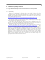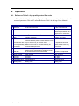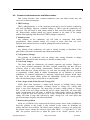
1
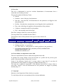
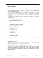
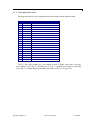
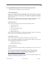
Argo data management
November 30th, 2005
ar-um-04-01
Argo quality control manual
Version 2.1
Table of contents
HISTORY
3
AUTHORS
3
1.
INTRODUCTION
4
2.
REAL-TIME QUALITY CONTROLS
5
2.1. ARGO R EAL-TIME Q UALITY CONTROL TEST PROCEDURES ON VERTICAL PROFILES
2.1.1. INTRODUCTION
2.1.2. QUALITY CONTROL TESTS
2.1.3. TESTS APPLICATION ORDER
2.2. ARGO R EAL-TIME Q UALITY CONTROL TEST PROCEDURES ON TRAJECTORIES
2.3. ARGO R EAL-TIME SALINITY ADJUSTMENT ON VERTICAL PROFILES
5
5
6
12
13
15
3.
16
DELAYED -MODE QUALITY CONTROLS
3.1. DELAYED - MODE PROCEDURES FOR PRESSURE
3.2. DELAYED - MODE PROCEDURES FOR TEMPERATURE
3.3. DELAYED - MODE PROCEDURES FOR SALIN ITY
3.3.1. INTRODUCTION
3.3.2. QUALITY CONTROL AND THE SEMI- AUTOMATIC PART
3.3.3. SPLITTING THE FLOAT SERIES AND LENGTH OF CALIBRATION WINDOW
3.3.4. THE PI EVALUATION PART
3.3.5. ASSIGNING ADJUSTED SALINITY, ERROR ESTIMATES , AND QC FLAGS
3.3.6. SUMMARY FLOWCHART
3.3.7. WHAT TO SAY IN THE SCIENTIFIC CALIBRATION SECTION OF THE NETCDF FILE
3.3.8. OTHER PARAMETERS IN THE NETCDF FILE
3.3.9. TIMEFRAME FOR AVAILABILITY OF DELAYED- MODE SALINITY DATA
3.3.10. REFERENCES
16
16
17
17
18
18
20
21
23
24
24
25
25
4.
26
4.1.
4.2.
APPENDIX
REFERENCE TABLE 2: ARGO QUALITY CONTROL FLAG SCALE
COMMON INSTRUMENT ERRORS AND FAILURE MODES
26
27
3
History
Date
01/01/2002
28/03/2003
08/06/2004
24/10/2003
07/10/2004
23/11/2004
26/11/2004
31/08/2005
17/11/2005
Comment
Creation of the document
Changed lower limit of temperature in Med to 10.0
Modified spike and gradient tests according to advice from Yasushi
and added inversion test
Real-time qc test 15 and 16 proposed at Monterey datamanagement meeting, test 10 removed
1. Real-time and delayed mode manuals merged in "Argo quality
control manual"
2. Frozen profile real time qc test 17 proposed at Southampton data
management meeting.
3. Deepest pressure real time qc test 18 proposed at Southampton
data management meeting.
4. Order list for the real time qc tests
5. "Regional Global Parameter Test" renamed "Regional range test",
test 7
6. Grey list naming convention and format, test 15
7. Real time qc on trajectories
§1 : new introduction from Annie Wong
§4 : delayed mode quality control manual from Annie Wong
§3 : update of summary flow for delayed mode qc chart p. 21
§2.2 : update on test 17, visual qc
§2.3 : added a section on real-time salinity adjustment.
§3.1 : added usage of SURFACE PRESSURE from APEX floats.
§3.3.5 : added some more guidelines for PSAL_ADJUSTED_QC =
'2'.
§3.3.8 : clarified that PROFILE_<PARAM>_QC should be
recomputed when <PARAM>_ADJUSTED_QC becomes available.
See p.24.
Authors
Annie Wong, Robert Keeley, Thierry Carval, and the Argo Data Management Team.
Argo data management
quality control manual
30/11/2004
4
1. Introduction
This document is the Argo quality control user’s manual.
The Argo data system has three levels of quality control.
•
The first level is the real-time system that performs a set of agreed checks on all
float measurements. Real-time data with assigned quality flags are available to
users within the 24-48 hrs timeframe.
•
The second level of quality control is the delayed-mode system.
•
The third level of quality control is regional scientific analyses of all float data
with other available data. The procedures for regional analyses are still to be
determined.
This document contains the description of the Argo real-time and delayed-mode
procedures.
Argo data management
quality control manual
30/11/2004
5
2. Real-time quality controls
2.1. Argo Real-time Quality Control Test Procedures on vertical profiles
2.1.1. Introduction
Because of the requirement for delivering data to users within 24 hours of the float
reaching the surface, the quality control procedures on the real-time data are limited and
automatic. The test limits are briefly described here. More detail on the tests can be found
in IOC Manuals and Guides #22 or at
http://www.meds-sdmm.dfo-mpo.gc.ca/ALPHAPRO/gtspp/qcmans/MG22/guide22_e.htm
Note that some of the test limits used here and the resulting flags are different from
what is described in IOC Manuals and Guides #22.
If data from a float fail these tests, those data will not be distributed on the GTS.
However, all of the data, including those having failed the tests, should be converted to
the appropriate netCDF format and forwarded to the Global Argo Servers.
Presently, the TESAC code form is used to send the float data on the GTS (see
http://www.meds-sdmm.dfo-mpo.gc.ca/meds/Prog_Int/J-COMM/J-COMM_e.htm).
This
code form only handles profile data and reports observations as a function of depth not
pressure. It is recommended that the UNESCO routines be used to convert pressure to
depth (Algorithms for computation of fundamental properties of seawater, N.P. Fofonoff
and R.C. Millard Jr., UNESCO Technical Papers in Marine Science #44, 1983). If the
position of a profile is deemed wrong, or the date is deemed wrong, or the platform
identification is in error then none of the data should be sent on the GTS. For other
failures, only the offending values need be removed from the TESAC message. The
appropriate actions to take are noted with each test.
Argo data management
quality control manual
30/11/2004
6
2.1.2. Quality control tests
1. Platform identification
Every centre handling float data and posting them to the GTS will need to prepare a
metadata file for each float and in this is the WMO number that corresponds to each float
ptt. There is no reason why, except because of a mistake, an unknown float ID should
appear on the GTS.
Action: If the correspondence between the float ptt cannot be matched to the correct
WMO number, none of the data from the profile should be distributed on the GTS.
2. Impossible date test
The test requires that the observation date and time from the float be sensible.
•
Year greater than 1997
•
Month in range 1 to 12
•
Day in range expected for month
•
Hour in range 0 to 23
•
Minute in range 0 to 59
Action: If any one of the conditions is failed, the date should be flagged as bad data and
none of the data from the profile should be distributed on the GTS.
3. Impossible location test
The test requires that the observation latitude and longitude from the float be sensible.
Action: If either latitude or longitude fails, the position should be flagged as bad data and
none of the data from the float should go out on the GTS.
•
Latitude in range -90 to 90
•
Longitude in range -180 to 180
4. Position on land test
The test requires that the observation latitude and longitude from the float be located in
an ocean.
Use can be made of any file that allows an automatic test to see if data are located on
land. We suggest use of at least the 5-minute bathymetry file that is generally available.
This is commonly called ETOPO5 / TerrainBase and can be downloaded from
http://www.ngdc.noaa.gov/mgg/global/global.html.
Action: If the data cannot be located in an ocean, the position should be flagged as bad
data and they should not be distributed on the GTS.
Argo data management
quality control manual
30/11/2004
7
5. Impossible speed test
Drift speeds for floats can be generated given the positions and times of the floats when
they are at the surface and between profiles. In all cases we would not expect the drift
speed to exceed 3 m/s. If it does, it means either a position or time is bad data, or a float
is mislabeled. Using the multiple positions that are normally available for a float while at
the surface, it is often possible to isolate the one position or time that is in error.
Action: If an acceptable position and time can be used from the available suite, then the
data can be sent to the GTS. Otherwise, flag the position, the time, or both as bad data
and no data should be sent.
6. Global range test
This test applies a gross filter on observed values for temperature and salinity. It needs to
accommodate all of the expected extremes encountered in the oceans.
•
Temperature in range -2.5 to 40.0 degrees C
•
Salinity in range 0.0 to 41.0 PSU
Action: If a value fails, it should be flagged as bad data and only that value need be
removed from distribution on the GTS. If temperature and salinity values at the same
depth both fail, both values should be flagged as bad data and values for depth,
temperature and salinity should be removed from the TESAC being distributed on the
GTS.
7. Regional range test
This test applies to only certain regions of the world where conditions can be further
qualified. In this case, specific ranges for observations from the Mediterranean and Red
Seas further restrict what are considered sensible values. The Red Sea is defined by the
region 10N,40E; 20N,50E; 30N,30E; 10N,40E and the Mediterranean Sea by the region
30N,6W; 30N,40E; 40N,35E; 42N,20E; 50N,15E; 40N,5E; 30N,6W.
Action: Individual values that fail these ranges should be flagged as bad data and
removed from the TESAC being distributed on the GTS. If both temperature and salinity
values at the same depth both fail, then values for depth, temperature and salinity should
be removed from the TESAC being distributed on the GTS.
Red Sea
•
Temperature in range 21.7 to 40.0
•
Salinity in range 0.0 to 41.0
Mediterranean Sea
•
Temperature in range 10.0 to 40
•
Salinity in range 0.0 to 40.0
8. Pressure increasing test
This test requires that the profile has pressures that are monotonically increasing
(assuming the pressures are ordered from smallest to largest).
Argo data management
quality control manual
30/11/2004
8
Action: If there is a region of constant pressure, all but the first of a consecutive set of
constant pressures should be flagged as bad data. If there is a region where pressure
reverses, all of the pressures in the reversed part of the profile should be flagged as bad
data. All pressures flagged as bad data and all of the associated temperatures and
salinities are removed from the TESAC distributed on the GTS.
9. Spike test
Difference between sequential measurements, where one measurement is quite different
than adjacent ones, is a spike in both size and gradient. The test does not consider the
differences in depth, but assumes a sampling that adequately reproduces the temperature
and salinity changes with depth. The algorithm is used on both the temperature and
salinity profiles.
Test value = | V2 - (V3 + V1)/2 | - | (V3 - V1) / 2 |
where V2 is the measurement being tested as a spike, and V1 and V3 are the values
above and below.
Temperature: The V2 value is flagged when
•
the test value exceeds 6.0 degree C. for pressures less than 500 db or
•
the test value exceeds 2.0 degree C. for pressures greater than or equal to 500 db
Salinity: The V2 value is flagged when
•
the test value exceeds 0.9 PSU for pressures less than 500 db or
•
the test value exceeds 0.3 PSU for pressures greater than or equal to 500 db
Action: Values that fail the spike test should be flagged as bad data and are removed
from the TESAC distributed on the GTS. If temperature and salinity values at the same
depth both fail, they should be flagged as bad data and the values for depth, temperature
and salinity should be removed from the TESAC being distributed on the GTS.
10. Top and bottom spike test: obsolete
11. Gradient test
This test is failed when the difference between vertically adjacent measurements is too
steep. The test does not consider the differences in depth, but assumes a sampling that
adequately reproduces the temperature and salinity changes with depth. The algorithm is
used on both the temperature and salinity profiles.
Test value = | V2 - (V3 + V1)/2 |
where V2 is the measurement being tested as a spike, and V1 and V3 are the values
above and below.
Temperature: The V2 value is flagged when
•
the test value exceeds 9.0 degree C. for pressures less than 500 db or
•
the test value exceeds 3.0 degree C. for pressures greater than or equal to 500 db
Argo data management
quality control manual
30/11/2004
9
Salinity : the V2 value is flagged when
•
the test value exceeds 1.5 PSU for pressures less than 500 db or
•
the test value exceeds 0.5 PSU for pressures greater than or equal to 500 db
Action: Values that fail the test (i.e. value V2) should be flagged as bad data and are
removed from the TESAC distributed on the GTS. If temperature and salinity values at
the same depth both fail, both should be flagged as bad data and then values for depth,
temperature and salinity should be removed from the TESAC being distributed on the
GTS.
12. Digit rollover test
Only so many bits are allowed to store temperature and salinity values in a profiling
float. This range is not always large enough to accommodate conditions that are
encountered in the ocean. When the range is exceeded, stored values rollover to the lower
end of the range. This rollover should be detected and compensated for when profiles are
constructed from the data stream from the float. This test is used to be sure the rollover
was properly detected.
•
Temperature difference between adjacent depths > 10 degrees C
•
Salinity difference between adjacent depths > 5 PSU
Action: Values that fail the test should be flagged as bad data and are removed from the
TESAC distributed on the GTS. If temperature and salinity values at the same depth both
fail, both values should be flagged as bad data and then values for depth, temperature and
salinity should be removed from the TESAC distributed on the GTS.
13. Stuck value test
This test looks for all measurements of temperature or salinity in a profile being identical.
Action: If this occurs, all of the values of the affected variable should be flagged as bad
data and are removed from the TESAC distributed on the GTS. If temperature and
salinity are affected, all observed values are flagged as bad data and no report from this
float should be sent to the GTS.
14. Density inversion
This test uses values for temperature and salinity at the same pressure level and computes
the density. The algorithm published in UNESCO Technical Papers in Marine Science
#44, 1983 (referred to earlier) should be used. Densities are compared at consecutive
levels in a profile.
Action: If the density calculated at the greater pressure is less than that calculated at the
lesser pressure, both the temperature and salinity values should be flagged as bad data.
Consequently, the values for depth, temperature and salinity at this pressure level should
be removed from the TESAC distributed on the GTS.
Argo data management
quality control manual
30/11/2004
10
15. Grey list
This test is implemented to stop the real-time dissemination of measurements from a
sensor that is not working correctly.
The grey list contains the following 7 items:
•
Float Id
•
Parameter : name of the grey listed parameter
•
Start date : from that date, all measurements for this parameter are flagged as bad
and probably bad
•
End date : from that date, measurements are not flagged as bad or probably bad
•
Flag : value of the flag to be applied to all measurements of the parameter
•
Comment : comment from the PI on the problem
•
DAC : data assembly center for this float
Each DAC manages a black list, sent to the GDACs.
The merged black-list is available from the GDACs.
The decision to insert a float parameter in the grey list comes from the PI.
Example:
Float Id
1900206
Parameter
PSAL
Start date
20030925
End date
Flag
3
Comment Dac
IF
•
Grey list format : ascii csv (comma separated values)
•
Naming convention : xxx_greylist.csv
xxx : DAC name (ex : aoml_greylist.csv, coriolis_greylist.csv, jma_greylist.csv)
•
PLATFORM,PARAMETER,START_DATE,END_DATE,QC,COMMENT,DAC
4900228,TEMP,20030909,,3,,AO
1900206,PSAL,20030925,,3,,IF
16. Gross salinity or temperature sensor drift
This test is implemented to detect a sudden and important sensor drift.
It calculates the average salinity on the last 100 dbar on a profile and the previous good
profile. Only measurements with good QC are used.
Action: if the difference between the 2 average values is more than 0.5 psu then all
measurements for this parameter are flagged as probably bad data (flag ‘3’).
The same test is applied for temperature: if the difference between the 2 average values is
more than 1 degree C then all measurements for this parameter are flagged as probably
bad data (flag ‘3’).
17. Visual QC
Subjective visual inspection of float values by an operator.
To avoid delays, this test is not mandatory before real-time distribution.
Argo data management
quality control manual
30/11/2004
11
18. Frozen profile test
This test can detect a float that reproduces the same profile (with very small deviations)
over and over again.
Typically the differences between 2 profiles are of the order of 0.001 for salinity and of
the order of 0.01 for temperature.
A. Derive temperature and salinity profiles by averaging the original profiles to get mean
values for each profile in 50dbar slabs (Tprof, T_previous_prof and Sprof,
S_previous_prof). This is necessary, because the floats do not sample at the same level
for each profile.
B. Substract the two resulting profiles for temperature and salinity to get absolute
difference profiles:
•
deltaT=abs(Tprof-T_previous_prof)
•
deltaS=abs(Sprof-S_previous_prof)
C. Derive the maximum, minimum and mean of the absolute differences for temperature
and salinity:
•
mean(deltaT), max(deltaT), min(deltaT)
•
mean(deltaS), max(deltaS), min(deltaS)
D. To fail the test, require that:
•
max(deltaT) < 0.3
•
min(deltaT) < 0.001
•
mean(deltaT) < 0.02
•
max(deltaS) < 0.3
•
min(deltaS) < 0.001
•
mean(deltaS) < 0.004
Action: if the profile fails the test, all measurements for this parameter are flagged as bad
data (flag ‘4’). If the float fails the test on 5 consecutive cycles, it is inserted in the greylist.
19. Deepest pressure test
This test requires that the profile has pressures that
DEEPEST_PRESSURE plus 5% 10% 100 dbar (to be defined).
are
not
higher
than
DEEPEST_PRESSURE value comes from the meta-data file of the float.
Action: If there is a region of incorrect pressures, all pressures and corresponding
measurements should be flagged as bad data (flag ‘4’). All pressures flagged as bad data
and all of the associated temperatures and salinities are removed from the TESAC
distributed on the GTS.
Argo data management
quality control manual
30/11/2004
12
2.1.3. Tests application order
The Argo real time QC tests are applied in the order described in the following table.
Order test number test name
1
2
3
4
5
6
7
8
9
10
11
12
13
14
15
16
17
18
19
19 Deepest pressure test
1 Platform Identification
2 Impossible Date Test
3 Impossible Location Test
4 Position on Land Test
5 Impossible Speed Test
6 Global Range Test
7 Regional Range Test
8 Pressure Increasing Test
9 Spike Test
10 Top and Bottom Spike Test : removed
11 Gradient Test
12 Digit Rollover Test
13 Stuck Value Test
14 Density Inversion
15 Grey List
16 Gross salinity or temperature sensor drift
18 Frozen profile
17 Visual QC
The QC flag value assigned by a test cannot override a higher value from a previous
test. Example: a QC flag ‘4’ (bad data) set by Test 11 (gradient test) cannot be decreased
to QC flag ‘3’ (bad data that are potentially correctable) set by Test 15 (grey list).
Argo data management
quality control manual
30/11/2004
13
2.2. Argo Real-time Quality Control Test Procedures on trajectories
The following tests are applied in real-time on trajectory data.
1. Platform identification
Every centre handling float data and posting them to the GTS will need to prepare a
metadata file for each float and in this is the WMO number that corresponds to each float
ptt. There is no reason why, except because of a mistake, an unknown float ID should
appear on the GTS.
Action: If the correspondence between the float ptt cannot be matched to the correct
WMO number, none of the data from the profile should be distributed on the GTS.
2. Impossible date test
The test requires that the observation date and time from the float be sensible.
•
Year greater than 1997
•
Month in range 1 to 12
•
Day in range expected for month
•
Hour in range 0 to 23
•
Minute in range 0 to 59
Action: If any one of the conditions is failed, the date should be flagged as bad data and
none of the data from the profile should be distributed on the GTS.
3. Impossible location test
The test requires that the observation latitude and longitude from the float be sensible.
Action: If either latitude or ol ngitude fails, the position should be flagged as bad data and
none of the data from the float should go out on the GTS.
•
Latitude in range -90 to 90
•
Longitude in range -180 to 180
4. Position on land test
The test requires that the observation latitude and longitude from the float be located in
an ocean.
Use can be made of any file that allows an automatic test to see if data are located on
land. We suggest use of at least the 5-minute bathymetry file that is generally available.
This is commonly called ETOPO5 / TerrainBase and can be downloaded from
http://www.ngdc.noaa.gov/mgg/global/global.html
Action: If the data cannot be located in an ocean, the position should be flagged as bad
data and they should not be distributed on the GTS.
Argo data management
quality control manual
30/11/2004
14
5. Impossible speed test
Drift speeds for floats can be generated given the positions and times of the floats when
they are at the surface and between profiles. In all cases we would not expect the drift
speed to exceed 3 m/s. If it does, it means either a position or time is bad data, or a float
is mislabeled. Using the multiple positions that are normally available for a float while at
the surface, it is often possible to isolate the one position or time that is in error.
Action: If an acceptable position and time can be used from the available suite, then the
data can be sent to the GTS. Otherwise, flag the position, the time, or both as bad data
and no data should be sent.
6. Global range test
This test applies a gross filter on observed values for temperature and salinity. It needs to
accommodate all of the expected extremes encountered in the oceans.
•
Temperature in range -2.5 to 40.0 degrees C
•
Salinity in range 0.0 to 41.0 PSU
Action: If a value fails, it should be flagged as bad data and only that value need be
removed from distribution on the GTS. If temperature and salinity values at the same
depth both fail, both values should be flagged as bad data and values for depth,
temperature and salinity should be removed from the TESAC being distributed on the
GTS.
7. Regional range test
This test applies to only certain regions of the world where conditions can be further
qualified. In this case, specific ranges for observations from the Mediterranean and Red
Seas further restrict what are considered sensible values. The Red Sea is defined by the
region 10N,40E; 20N,50E; 30N,30E; 10N,40E and the Mediterranean Sea by the region
30N,6W; 30N,40E; 40N,35E; 42N,20E; 50N,15E; 40N,5E; 30N,6W.
Action: Individual values that fail these ranges should be flagged as bad data and
removed from the TESAC being distributed on the GTS. If both temperature and salinity
values at the same depth both fail, then values for depth, temperature and salinity should
be removed from the TESAC being distributed on the GTS.
Red Sea
•
Temperature in range 21.7 to 40.0
•
Salinity in range 0.0 to 41.0
Mediterranean Sea
•
Temperature in range 10.0 to 40
•
Salinity in range 0.0 to 40.0
Argo data management
quality control manual
30/11/2004
15
2.3. Argo Real-time Salinity Adjustment on vertical profiles
When delayed-mode salinity adjustment (see Section 3.3) becomes available for a
float, real-time data assembly centres will extract the adjustment from the latest D*.nc
file as an additive constant, and apply it to new salinity profiles. (If a better correction is
available in real-time, DACs can use that instead.) In this manner, intermediate-quality
salinity profiles will be available to users in real-time.
The values of this real-time adjustment will be recorded in PSAL_ADJUSTED.
PSAL_ADJUSTED_QC will be filled with the same values as PSAL_QC.
PSAL_ADJUSTED_ERROR and all parameters in the SCIENTIFIC CALIBRATION
section of the netCDF files will be filled with FillValue.
A HISTORY record will be appended to the HISTORY section indicating that realtime salinity adjustment has been made.
DATA_MODE will record ‘A’.
When available, real-time adjusted values are distributed to the GTS, instead of the
original values.
Argo data management
quality control manual
30/11/2004
16
3. Delayed-mode quality controls
3.1. Delayed-mode procedures for pressure
Delayed-mode qc for PRES is done by subjective assessment of vertical profile plots
of TEMP vs. PRES, and PSAL vs. PRES. This assessment should be done in relation to
measurements from the same float, as well as in relation to nearby floats and historical
data. The assessment should aim to identify: (a) erroneous data points that cannot be
detected by the real-time qc tests, and (b) vertical profiles that have the wrong shape.
Bad data points identified by visual inspection from delayed-mode analysts are
recorded with PRES_ADJUSTED_QC = ‘4’. For these bad data points,
TEMP_ADJUSTED_QC and PSAL_ADJUSTED_QC should also be set to ‘4’. Please
note that whenever PARAM_ADJUSTED_QC = ‘4’,
•
PARAM_ADJUSTED = FillValue;
•
PARAM_ADJUSTED_ERROR = FillValue.
Some float groups that have extra information on surface pressure can perform
delayed-mode adjustments for PRES, by comparing measured surface pressure and 0.0
dbar. The results are recorded in PRES_ADJUSTED, PRES_ADJUSTED_ERROR, and
PRES_ADJUSTED_QC. Please note that there is no need to recompute PSAL when
PRES is adjusted in delayed-mode. Any salinity offset that may result from PRES
adjustments can be reflected in PSAL_ADJUSTED.
For APEX floats, use next cycle “SURFACE PRESSURE” to adjust PRES if there is
evidence that the values reported in “SURFACE PRESSURE” represent significant
sensor-related drift or offset.
PRES_ADJUSTED, PRES_ADJUSTED_ERROR, PRES_ADJUSTED_QC should be
filled even when no adjustment is made. In these cases, PRES_ADJUSTED_ERROR can
be the manufacturer’s calibration uncertainty, or uncertainty provided by the PI.
Please use the CALIB section in the netCDF files to record the source of the error
estimates and any other scientific calibration comments (e.g. surface PRES is
automatically reset to zero).
3.2. Delayed-mode procedures for temperature
Delayed-mode qc for TEMP is done by subjective assessment of vertical profile plots
of TEMP vs. PRES, and PSAL vs. TEMP. This assessment should be done in relation to
measurements from the same float, as well as in relation to nearby floats and historical
data. The assessment should aim to identify: (a) erroneous data points that cannot be
detected by the real-time qc tests, and (b) vertical profiles that have the wrong shape.
Bad data points identified by visual inspection from delayed-mode analysts are
recorded with TEMP_ADJUSTED_QC = ‘4’. Please note that whenever
PARAM_ADJUSTED_QC = ‘4’,
•
PARAM_ADJUSTED = FillValue;
•
PARAM_ADJUSTED_ERROR = FillValue.
Argo data management
quality control manual
30/11/2004
17
TEMP_ADJUSTED, TEMP_ADJUSTED_ERROR, TEMP_ADJUSTED_QC should
be filled even when no adjustment is made. In these cases, TEMP_ADJUSTED_ERROR
can be the manufacturer’s quoted accuracy at deployment of float.
Please use the CALIB section in the netCDF files to record the source of the error
estimates and any other scientific calibration comments.
3.3. Delayed-mode procedures for salinity
3.3.1. Introduction
Delayed-mode qc for PSAL described in this section are specifically for checking
sensor drifts and offsets. Analysts should be aware that there are other instrument errors,
and should attempt to identify and adjust them in delayed-mode. If a measurement has
been adjusted for more than one instrument error, analysts should attempt to propagate
the uncertainties from all the adjustments.
The free-moving nature of profiling floats means that most float salinity measurements
are without accompanying in-situ “ground truth” values for absolute calibration (such as
those afforded by shipboard CTD measurements). Therefore Argo delayed-mode
procedures for checking sensor drifts and offsets in salinity rely on reference datasets and
statistical methods. However, since the ocean has inherent spatial and temporal
variabilities, these drift and offset adjustments are subject to statistical uncertainties.
Users therefore should include the supplied error estimates in their usage of Argo
delayed-mode salinity data.
Two methods are available for detecting sensor drifts and offsets in float salinity, and
for calculating adjustment estimates and related uncertainties:
1. Wong, Johnson, Owens (2003) estimates background salinity on a set of fixed
standard isotherms, then calculates drifts and offsets by time-varying weighted least
squares fits between vertically-interpolated float salinity and estimated background
salinity. This method suits float data from open tropical and subtropical oceans. For the
related software, please contact Annie Wong at [email protected].
2. Boehme and Send (2005) takes into account planetary vorticity in its estimates of
background salinity, and chooses a set of desirable isotherms for calculations. This
method suits float data from oceans with high spatial and temporal variabilities, where
water mass distribution is affected by topographic barriers, and where multiple water
masses exist on the same isotherm. For the related software, please contact Lars Boehme
at [email protected].
Both methods require an adequate reference database and an appropriate choice of
spatial and temporal scales, as well as input of good/adjusted float pressure, temperature,
position, and date of sampling. Therefore analysts should first check the reference
database for adequacy and determine a set of appropriate spatial and temporal scales
before using these methods. Operators should also ensure that other float measurements
(PRES, TEMP, LATITUTDE, LONGITUDE, JULD) are accurate or adjusted before
they deal with float salinity. See Secions 3.1 and 3.2 for delayed-mode procedures for
PRES and TEMP.
Argo data management
quality control manual
30/11/2004
18
3.3.2. Quality control and the semi-automatic part
The real-time qc procedures (described in Section 2) issue a set of qc flags that warns
users of the quality of the float salinity. These are found in the variable PSAL_QC. Float
salinity with PSAL_QC = ‘4’ are bad data that are in general unadjustable. However,
delayed-mode operators can evaluate the quality and adjustability of these bad data if
they have a reason to do so. Please refer to Section 4.1 for definitions of the Argo qc
flags in real-time.
In delayed-mode, float salinity that have PSAL_QC = ‘1’, ‘2’ or ‘3’ are further
examined. Anomalies in the relative vertical salinity profile, such as measurement spikes
and outliers that are not detected in real-time, are identified. Of these anomalies, those
that will skew the least squares fit in the computation for drift and offset adjustments are
excluded from the float series for evaluation of drifts and offsets. These measurements
are considered unadjustable in delayed-mode.
Float salinity that are considered adjustable in delayed-mode are assembled into time
series, or float series. Sufficiently long float series are compared with statistical
recommendations and associated uncertainties to check for sensor drifts and offsets.
These statistical recommendations and associated uncertainties are obtained by the
accepted methods listed in Section 3.3.1, in conjunction with appropriate reference
datasets. These methods are semi-automatic and have quantified uncertainties.
Drifts and offsets can be identified in the trend of ∆S over time, where ∆S is the
difference in salinity between float series and statistical recommendations. If ? S = a + bt
where t is time, then a is the offset and b is the drift. Note that these drifts and offsets can
be sensor-related, or they can be due to real ocean events. PI evaluation is needed to
distinguish between sensor errors and real ocean events.
3.3.3. Splitting the float series and length of calibration window
If a float exhibits changing behaviour during its lifetime, the float series should be
split into separate segments according to the different behaviours, so that one float series
segment does not contaminate the other during the least squares fit process (e.g. the
slowly-fouling segment does not contaminate the stable segment).
Argo data management
quality control manual
30/11/2004
19
The following is a step-by-step guide on how to deal with float series with changing
behaviours.
1). Identify different regimes in the float series. These can be:
•
Stable measurements (no sensor drift), including constant offsets.
•
Sensor drift with a constant drift rate.
•
Transition phase where drift rate changes rapidly e.g. (a) ‘elbow region’
between stable measurements and constant drift; (b) initial biocide wash-off.
•
Spikes.
2). Split the float series into discrete segments according to these different regimes or
when there are too many missing cycles. Here is an example.
?S
Constant offset
Discontinuity (no
transition phase)
Sensor drift with a
constant drift rate
Transition phase
Spike
Stable
time
3). Choose length of sliding calibration window for each segment. These can be:
• Long window (+/- 6 months or greater) for the stable regime, or highly variable
regimes where a long window is required to average over oceanographic variability to
detect slow sensor drift, or period of constant drift rate.
•
Short window (can be as short as +/- 10 days) for the transition phase.
•
Zero length window for spikes. That is, adjust single profile.
4). Select temperature levels for exclusion from least squares fit (e.g. seasonal mixed
layer, highly variable water masses).
Argo data management
quality control manual
30/11/2004
20
5). Calculate proposed adjustment for each segment. The assembled proposed
adjustments for the entire float series should be continuous and piecewise-linear within
error bars, except where the delayed-mode operator believes there is a genuine
discontinuity.
In general, the delayed-mode operator should aim to use as long a calibration window
as possible, because a long calibration window (where the least squares fit is calculated
over many cycles) will average over oceanographic noise and thus give a stable
calibration. Hence splitting the float series into short segments is to be avoided (short
segments mean short calibration windows, hence unstable calibrations).
3.3.4. The PI evaluation part
The PI (here, PI means Principal Investigator, or responsible persons assigned by the
PI) should first check that the statistical recommendations are appropriate. This is
because the semi-automatic methods cannot distinguish ocean features such as eddies,
fronts, and water mass boundaries. Near such ocean features, semi-automatic statistical
methods are likely to produce erroneous estimations. The associated uncertainties reflect
the degree of local variability as well as the sparsity of reference data used in the
statistical estimations. However, these associated uncertainties are sensitive to the choice
of scales. Hence the PI also needs to determine that the associated uncertainties are
realistic.
The PI then determines whether the proposed statistical adjustment is due to sensor
malfunction or ocean variability. Care should be taken to not confuse real ocean events
with sensor drifts and offsets. This is done by inspecting as long a float series as possible,
and by evaluating all available independent information. Some of the diagnostic tools can
include:
• Inspecting the trend of ∆S over time. Trends that reverse directions, or oscillate, are
difficult to explain in terms of systematic sensor malfunction. These are often caused by
the float sampling oceanographic features (e.g. eddies, fronts, etc.) that are not
adequately described in the reference database.
• Visual check of float trajectory with reference to oceanographic features such as
eddies and rings that can introduce complications to the semi-automatic methods.
• Inspecting contour plots of float salinity anomaly time series. Systematic sensor
malfunction should show up as salinity anomalies over several water masses.
• Using other independent oceanographic atlases to anticipate water mass changes that
can occur along a float’s path, and that can be misinterpreted as sensor malfunction.
• Inspecting residuals from objective maps.
• Cross-checking with nearby stable floats in cases of suspect sensor calibration offset.
If the PI is confident that sensor malfunction has occurred, then the threshold for
making an adjustment is when ?S is greater than 2 times whatever is reported in
PSAL_ADJUSTED_ERROR. By default this will be the error from the statistical
methods, but the PI can provide an alternative estimate of uncertainty if they have a basis
for doing so. Note that this guideline is to help the PI in deciding whether a slope or
offset is statistically significant, and so should be used to evaluate the entire float
segment being fitted, and not to single points.
Argo data management
quality control manual
30/11/2004
21
The lower bound on the size of an adjustment is the instrument accuracy. At present,
there is no upper bound for the magnitude of salinity adjustment.
In cases where the float series has been split into separate segments, the PI must
ensure that the assembled adjustment for the entire float series is continuous within error
bars, except where the PI believes there is a genuine discontinuity (see Step 5 in Section
3.3.3). This is to ensure that no artificial jump is introduced where the separate segments
join. Adjustment continuity between separate float segments can be achieved by making
adjustment in the transition phase even though the adjustment is below the 2 times error
threshold limit.
In the following example, the float series experiences sensor drift after a stable period.
The float series has been split for calibration. However, the float series has no
discontinuity, so the final assembled adjustment should be continuous. Adjustment
continuity is achieved by using model (a) and not (b).
3.3.5. Assigning adjusted salinity, error estimates, and qc flags
After evaluating all available information, the PI then assigns adjusted salinity values,
error estimates, and delayed-mode qc flags. In Argo netcdf files, these are found
respectively in the parameters PSAL_ADJUSTED, PSAL_ADJUSTED_ERROR, and
PSAL_ADJUSTED_QC. Please refer to Section 4.1 for definitions of the Argo qc flags
in delayed-mode.
The original float salinity and real-time qc flags remain in the parameters PSAL and
PSAL_QC, and are never altered in delayed-mode.
A Matlab-based graphical user interface for interacting with Argo netcdf files has been
developed by John Gilson at Scripps Institute of Oceanography. Please contact
[email protected].
The following is a set of guidelines for assigning values to PSAL_ADJUSTED,
PSAL_ADJUSTED_ERROR and PSAL_ADJUSTED_QC in Argo netcdf files.
When no delayed-mode qc is available
For example, when the netcdf file is still in real-time mode, or when there is no
LATITUDE, LONGITUDE, or JULD (hence no statistical recommendation available).
Argo data management
quality control manual
30/11/2004
22
•
PSAL_ADJUSTED = FillValue;
•
PSAL_ADJUSTED_ERROR = FillValue;
•
PSAL_ADJUSTED_QC = FillValue.
For float salinity that are considered unadjustable in delayed-mode
For example, large spikes, or extreme behaviour where the relative vertical T-S shape
does not match good data. These measurements are unadjustable.
•
PSAL_ADJUSTED = FillValue;
•
PSAL_ADJUSTED_ERROR = FillValue;
•
PSAL_ADJUSTED_QC = ‘4’.
For float salinity that are considered adjustable in delayed-mode
These measurements have a relative vertical T-S shape that is close to good data. They
are evaluated and adjusted for sensor drifts, offsets, and any other instrument errors.
i). When no adjustment is needed,
•
PSAL_ADJUSTED = PSAL (original value);
•
PSAL_ADJUSTED_ERROR = max [statistical uncertainty, instrument accuracy],
or uncertainty provided by PI;
•
PSAL_ADJUSTED_QC = ‘1’, ‘2’, or ‘3’.
ii). When an adjustment has been applied,
•
PSAL_ADJUSTED = value recommended by statistical analyses, or adjustment
provided by PI;
•
PSAL_ADJUSTED_ERROR = max [statistical uncertainty, instrument accuracy],
or uncertainty provided by PI;
•
PSAL_ADJUSTED_QC = ‘1’, ‘2’, or ‘3’.
iii). When the PI determines that float salinity are bad and unadjustable,
•
PSAL_ADJUSTED = FillValue;
•
PSAL_ADJUSTED_ERROR = FillValue;
•
PSAL_ADJUSTED_QC = ‘4’.
The following are some cases where a flag ‘2’ should be assigned
•
Adjustment is based on unsatisfactory reference database.
•
Adjustment is based on a short calibration window (because of sensor behaviour
transition, or end of sensor life) and therefore may not be stable.
•
Evaluation is based on insufficient information.
•
Sensor is unstable (e.g. magnitude of adjustment is too big, or sensor has
undergone too many sensor behaviour changes) and therefore data are inherently
of mediocre quality.
•
When a float exhibits problems with its pressure measurements.
Argo data management
quality control manual
30/11/2004
23
3.3.6. Summary flowchart
Argo salinity sensor drift & offset QC procedures
Manual evaluation to detect anomalies on the relative profile, such as spikes,
that are not detected in RT.
Remove anomalies that may skew the drift/offset correction.
Do not use in least squares fit.
PSAL_ADJUSTED
= FillValue
PSAL_ADJUSTED_ERROR
= FillValue
PSAL_ADJUSTED_QC = 4
Use in least squares fit.
Use accepted methods and reference database, split series and select
appropriate length for the sliding window, to calculate recommended
salinity adjustments.
PI evaluation - consider long time series
and other supporting information to determine
whether sensor malfunction has happened.
No sensor error has been detected, or sensor drift
and/or offset is not significant
Sensor drift and/or offset has been detected
and is significant
< max [ 2 x statistical uncertainty, instrument accuracy ]
> max [ 2 x statistical uncertainty, instrument accuracy ]
Apply adjustment,
or declare unadjustable.
No adjustment needed.
PSAL_ADJUSTED = PSAL (original value)
PSAL_ADJUSTED_ERROR
= max [statistical uncertainty, instrument accuracy],
or uncertainty provided by PI
PSAL_ADJUSTED_QC = 1, 2 or 3
PSAL_ADJUSTED
= value recommended by statistical analyses, or
adjustment provided by PI
PSAL_ADJUSTED_ERROR
= max [statistical uncertainty, instrument accuracy],
or uncertainty provided by PI
PSAL_ADJUSTED_QC = 1, 2 or 3
OR
Last update :19-Apr-05
Argo data management
PSAL_ADJUSTED
= FillValue
PSAL_ADJUSTED_ERROR
= FillValue
PSAL_ADJUSTED_QC = 4
quality control manual
30/11/2004
24
3.3.7. What to say in the scientific calibration section of the netcdf file
Within each single-profile Argo netcdf file is a scientific calibration section that
records details of delayed-mode adjustments. In this scientific calibration section, for
every parameter listed in PARAMETER (PRES, TEMP, PSAL), there are four fields to
record scientific calibration details:
•
SCIENTIFIC_CALIB_EQUATION;
•
SCIENTIFIC_CALIB_COEFFICIENT;
•
SCIENTIFIC_CALIB_COMMENT;
•
CALIBRATION_DATE.
In cases where no adjustment has been made, SCIENTIFIC_CALIB_EQUATION and
SCIENTIFIC_CALIB_COEFFICIENT shall be filled by their respective FillValue.
SCIENTIFIC_CALIB_COMMENT shall contain wordings that describe the evaluation,
e.g. “No adjustment is needed.”
In cases where adjustments have been made, examples of wordings for PSAL can be:
SCIENTIFIC_CALIB_EQUATION: “PSAL_ADJUSTED = PSAL + ? S, where ? S is
calculated from a potential conductivity (ref to 0 dbar) multiplicative adjustment term r.”
SCIENTIFIC_CALIB_COEFFICIENT: “r = 0.9994 (± 0.0001), vertically averaged ? S =
− 0.025 (± 0.003).”
SCIENTIFIC_CALIB_COMMENT: “Sensor drift detected. Adjusted float salinity to
statistical recommendation as in WJO (2003), with WOD2001 as the reference database.
Mapping scales used are 8/4, 4/2. Length of sliding calibration window is +/- 20 profiles”
The PI is free to use any wordings he/she prefers. Just be precise and informative.
Regardless of whether an adjustment has been made, the date of calibration of each
parameter (PRES, TEMP, PSAL) should be recorded in CALIBRATION_DATE.
3.3.8. Other parameters in the netcdf file
A history record should be appended to the HISTORY section of the netcdf file to
indicate that the netcdf file has been through the delayed-mode process. Please refer to
the Argo User’s Manual (§5 “Using the History section of the Argo netCDF Structure”)
on usage of the History section.
The parameter DATA_MODE should record ‘D’.
The parameter DATA_STATE_INDICATOR should record ‘2C’.
The parameter DATE_UPDATE should record the date of last update of the netcdf file.
The parameters PROFILE_<PARAM>_QC
<PARAM>_ADJUSTED_QC becomes available.
should
be
recomputed
when
Lastly, the name of the single-profile Argo netcdf file is changed from R*.nc to D*.nc.
Argo data management
quality control manual
30/11/2004
25
3.3.9. Timeframe for availability of delayed-mode salinity data
The statistical methods used in the Argo delayed-mode process for checking sensor
drifts and offsets in salinity require the accumulation of a time series for reliable
evaluation of the sensor trend. Timeframe for availability of delayed-mode salinity data
is therefore dependent on the sensor trend. Some floats need a longer time series than
others for stable calibration. Thus delayed-mode salinity data for the most recent profile
may not be available until sufficient subsequent profiles have been accumulated. The
default length of time series for evaluating sensor drift is 12 months (6 months before
and 6 months after the profile). This means that in general, the timeframe of availability
of drift-adjusted delayed-mode salinity data is 6+ months after a profile is sampled.
Users should also be aware that changes may be made to delayed-mode files at any
time by DACs and delayed-mode operators. For example, delayed-mode files may be
revised when new CTD or float data become available after the original delayed-mode
assessment and adjustment. The date of latest adjustment of a parameter can be found in
CALIBRATION_DATE.
Anytime an Argo file is updated for any reason, the DATE_UPDATE variable will
reflect the date of the update. The "profile index file" on the GDACs contains the
DATE_UPDATE information (along with other information) for every file on the
GDACs and can be used to monitor updates. The profile index file is maintained in the
top-level GDAC directory and is named "ar_index_global_prof.txt"; index files also exist
for the meta-data and trajectory files.
3.3.10.
References
Böhme, L. and U. Send, 2005: Objective analyses of hydrographic data for referencing
profiling float salinities in highly variable environments, Deep-Sea Research II, 52/3-4,
651-664.
Wong, A.P.S., G.C. Johnson, and W.B. Owens, 2003: Delayed-mode calibration of
autonomous CTD profiling float salinity data by θ-S climatology. Journal of
Atmospheric and Oceanic Technology, 20, 308-318.
Argo data management
quality control manual
30/11/2004
26
4. Appendix
4.1. Reference Table 2: Argo quality control flag scale
This table describes the Argo qc flag scales. Please note that this table is used for all
measured parameters. This table is named Reference Table 2 in the Argo User’s Manual.
n Meaning
No QC was
0 performed
Real-time comment
Delayed-mode comment
No QC was performed
1 Good data
Probably good
2 data
All Argo real-time QC tests passed.
No QC was performed
The adjusted value is
statistically consistent and a
statistical error estimate is
supplied.
Probably good data
Test 15 or Test 16 or Test 17 failed and all other
real-time QC tests passed. These data are not to
be used without scientific correction. A flag ‘3’
Probably bad data may be assigned by an operator during
that are potentially additional visual QC for bad data that may be
3 correctable
corrected in delayed-mode.
Data have failed one or more of the real-time QC
tests, excluding Test 16. A flag ‘4’ may be
assigned by an operator during additional visual
4 Bad data
QC for bad data that are uncorrectable.
Probably good data
5
6
7
8
9
Value changed
Not used
Not used
Interpolated value
Missing value
Value changed
Not used
Not used
Interpolated value
Missing value
Argo data management
Value changed
Not used
Not used
Interpolated value
Missing value
quality control manual
An adjustment has been
applied, but the value may
still be bad.
Bad data. Not adjustable.
30/11/2004
27
4.2. Common instrument errors and failure modes
This section describes some common instrument errors and failure modes that will
cause error in float measurements.
1. TBTO leakage
TBTO (tributyltinoxide) is a wide spectrum poison that is used to protect conductivity
cells from biofouling. However, accidental leakage of TBTO onto the conductivity cell
can occur. This will result in fresh salinity offsets in float series that usually gets washed
off. Delayed-mode analysts should pay special attention to the shape of the salinity
profiles at the beginning of the float series if TBTO leakage is suspected.
2. Pollution events
Any pollution on the conductivity cell will result in erroneously fresh salinity
measurements. When pollution washes off, reversal of sensor drift trend can occur.
Delayed-mode analysts need to be careful in splitting float series in such cases.
3. Ablation events
Any ablation of the conductivity cell, such as etching, scouring, or dissolution of the
glass surface, will result in erroneously salty salinity measurements.
4. Cell geometry changes
The geometry of conductivity cells can change, thus causing electrodes to change
distance. This will result in either an increase or decrease in salinity values.
5. Cell circuit changes
The circuit within the conductivity cell contains capacitors and resistors. Changes to
any of these electrical components will affect electrical conductivity and thus will give
erroneous (fresh or salty) salinity measurements. Electrical complication can result in
sensor drifts that have varying drift rates (e.g. drift rates can change from slow and linear
to exponential). Usually jumps in salinity measurements are an indication of electrical
malfunction. If electrical complication is suspected, delayed-mode analysts should check
the shape of the vertical salinity profiles for adjustability. Usually the vertical profiles
after a measurement jump are wrong and so are uncorrectable.
6. Low voltage at end of float life, and “Energy Flu”
APEX floats often experience a sudden rapid decrease in available battery energy
reserves. This premature exhaustion of battery, known as “Energy Flu”, usually starts
about 2 years after deployment. The sharp drop in battery voltage related to “Energy
Flu”, as well as the low voltage towards the end of a float’s natural life, will cause spiky
erratic measurements that will make it difficult for delayed-mode analysts to determine
where to split the float series and how to fit a slope. Towards the end of float life, low
voltage will result in large drift, followed by death. “Energy Flu” will cause spikes that
get worse and more frequent, also followed by death.
7. Druck sensor problem
About 4% of SBE41s have experienced the Druck pressure sensor defect. SeaBird has
fixed this problem, so this feature is only included in this section for identifying the
profiles that have been affected. The Druck sensor problem is caused by oil getting into
the pressure sensor, causing the sensor to report either PRES ~ (+) 3000 dbar or (-) 3000
dbar. The pressure sensor tries to adjust the piston to the “fooled” pressure, and so
Argo data management
quality control manual
30/11/2004
28
progressively becomes a surface drifter. The problem usually starts with a profile that
reports measurements from very close-together depth levels. Both temperature and
salinity measurements are useless from that stage onward.
8. Incorrect pressure sensor coefficient
Incorrect scaling coefficient in the pressure sensor will give anomalous T-S curves at
depth. The T-S relation will look acceptable, but at depth it will look as if the float is
sampling an anomalous water mass relative to nearby floats. Delayed-mode analysts
should try to re-scale pressure measurements (e.g. PRES’ = PRES * X) to see whether
the T-S curve can be recovered. Air bubbles in the pressure transducer can also cause
erroneous pressure measurements that are visible as anomalous T-S curves.
9. Thermal inertia lag
Salinity reported immediately after a float has crossed a strong thermal gradient can be
in error as a result of conductivity cell thermal mass. This error arises because of heat
exchange between the conductivity cell and the water within it. A float that transits from
cold to warm water can result in fresh error, and from warm to cold in salty error. These
errors can exceed 0.01 (PSS-78) for strong thermal gradients, and sometimes result in
unstable fresh spikes at the base of the mixed layer.
Argo data management
quality control manual
30/11/2004