Download Structural Analysis Software Applications

Structural Analysis Software Applications
Science and Technology Support
High Performance Computing
Ohio Supercomputer Center
1224 Kinnear Road
Columbus, OH 43212-1163
2KLR6XSHUFRPSXWHU&HQWHU
Table of Contents
Introduction
LS-DYNA Program
ABAQUS Program
ANSYS Program
2KLR6XSHUFRPSXWHU&HQWHU
6WUXFWXUDO$QDO\VLV6RIWZDUH
$SSOLFDWLRQV
2
Introduction
Course Objectives
OSC Structures Packages
OSC Computer Systems
Access to OSC Systems
Enabling X-Window Graphics
2KLR6XSHUFRPSXWHU&HQWHU
6WUXFWXUDO$QDO\VLV6RIWZDUH
$SSOLFDWLRQV
3
Course Objectives
1) Provide the user with information necessary to select which software
package is best suited for a given problem.
2) Review basic functionality of each package
This will be accomplished by:
⇒ Review the modeling capabilities of each package
⇒ Learn how to configure graphic sessions from OSC to your local
workstations
⇒ Examine the basic functionality of pre and post processors through
lecture, examples and labs
⇒ Learn how to execute analysis in batch mode
⇒ Identify important sources of documentation and information
2KLR6XSHUFRPSXWHU&HQWHU
6WUXFWXUDO$QDO\VLV6RIWZDUH
$SSOLFDWLRQV
4
OSC Structures Packages
1$675$1
$%$4866WDQGDUG
$%$486([SOLFLW
$%$4863RVW
$%$4869LHZHU
$%$486&$(
$16<6
2KLR6XSHUFRPSXWHU&HQWHU
/LYHUPRUH
6RIWZDUH
7HFKQRORJ\
&RUSRUDWLRQ
/6'<1$'
/61,.('
/6,1*5,'
/67$8586
/63267
6WUXFWXUDO$QDO\VLV6RIWZDUH
$SSOLFDWLRQV
5
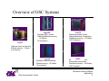
Overview of OSC Systems
Scalable RISC system
Distributed/Shared memory
16 Gbytes
32 processors
Massively parallel system
High performance components
Distributed memory - 16 Gbytes
128 Processors
Scalable vector processing
Shared memory - 16 Gbytes
16 processors
Massively parallel system
Commodity components
Distributed memory - 64 Gbytes
128 Processors
High end vector processing
Shared memory - 1 Gbyte
4 processors
2KLR6XSHUFRPSXWHU&HQWHU
6WUXFWXUDO$QDO\VLV6RIWZDUH
$SSOLFDWLRQV
6
Software by System
Cray T90 (osca.osc.edu) - Shared memory vector machine
ABAQUS v5.7
LS-DYNA v 940.1a & LS-DYNA v 950
NASTRAN v 70.5
ANSYS v 5.5
Cray T3E (t3e.osc.edu) - Distributed memory MPP machine
MPPDYNA v 940.0 beta
SGI Origin 2000 (origin.osc.edu) - CCNUMA memory machine
ABAQUS v5.7-4, v5.8-1and v5.8-17
LS-DYNA v 940.0, 940.1a, 950.0
ANSYS v 5.5
2KLR6XSHUFRPSXWHU&HQWHU
6WUXFWXUDO$QDO\VLV6RIWZDUH
$SSOLFDWLRQV
7
Software by System
Cray SV1 (oscb.osc.edu) - Shared memory vector machine
LS-DYNA v 950
OSC/SGI Intel Linux Cluster (oscbw.osc.edu) - Distributed
memory MPP machine
LS-DYNA v 940.2
2KLR6XSHUFRPSXWHU&HQWHU
6WUXFWXUDO$QDO\VLV6RIWZDUH
$SSOLFDWLRQV
8
Access to OSC systems
• All access is remote
telnet, ssh
• Local machine => (the machine you are sitting at)
• Remote machine => The OSC supercomputer (T90, T3E or Origin)
• X-Window Graphics
– Standard on Unix workstations
– Need extra software for PC or Mac
• Pre and post processors may be run interactively
• Solvers must be run in batch mode
2KLR6XSHUFRPSXWHU&HQWHU
6WUXFWXUDO$QDO\VLV6RIWZDUH
$SSOLFDWLRQV
9
Enabling X-Window Graphics
Command
xhost + origin.osc.edu
w -W (on Origin 2000)
Description
-This command is executed on your local machine. It
authorizes the OSC computer to display graphics on your
local workstation. You must issue this command for each
computer you want to use. Only for UNIX workstations.
-This command is executed on the remote machine. The
purpose is to get your local IP address.
who (on T90 and T3E)
jimg
ttyq32
3:48pm
oscnet108.osc.edu
-”echo $SHELL” will tell you which shell you are in
echo $SHELL
if csh
setenv DISPLAY oscnet108.osc.edu:0.0
if ksh
-This command is executed on the remote machine. It
instructs the remote computer where to send the display.
The local name was obtained from the 2nd line printed by
the ‘w -W’ command.
export DISPLAY=oscnet108.osc.edu:0.0
2KLR6XSHUFRPSXWHU&HQWHU
6WUXFWXUDO$QDO\VLV6RIWZDUH
$SSOLFDWLRQV
10
LS-DYNA Package
LS-DYNA Modeling Features
LS-DYNA Components
LS-DYNA Documentation
Model Generation with LS-INGRID
Running LS-DYNA Solver on T90 & SV1
Running LS-DYNA Solver on T3E
Running LS-DYNA Solver on Origin
LS-TAURUS Post Processor
LS-POST Post Processor
2KLR6XSHUFRPSXWHU&HQWHU
6WUXFWXUDO$QDO\VLV6RIWZDUH
$SSOLFDWLRQV
11
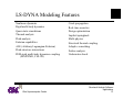
LS-DYNA Modeling Features
Nonlinear dynamics
Rigid multi-body dynamics
Quasi-static simulations
Thermal analysis
Fluid analysis
Eulerian capabilities
ALE (Arbitrary Lagrangian-Eulerian)
Fluid-structure interactions
FEM-rigid multi-body dynamics coupling
(MADYMO, CAL3D)
2KLR6XSHUFRPSXWHU&HQWHU
Crack propagation
Real-time acoustics
Design optimization
Implicit springback
Multi-physics
Structural thermal coupling
Adaptive remeshing
Failure analysis
Underwater shock
6WUXFWXUDO$QDO\VLV6RIWZDUH
$SSOLFDWLRQV
12
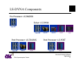
LS-DYNA Components
3UH3URFHVVRU/6,1*5,'
6ROYHU/6'<1$
3RVW3URFHVVRU/67$8586
2KLR6XSHUFRPSXWHU&HQWHU
3RVW3URFHVVRU/63267
6WUXFWXUDO$QDO\VLV6RIWZDUH
$SSOLFDWLRQV
13
LS-DYNA Documentation
• Documentation is available on-line in Adobe .pdf format
http://oscinfo.osc.edu/software/
Click on Origin 2000
Click on LSDYNA
Manuals are the same for all platforms
LS-DYNA User’s Manual (Structural version)
LS-DYNA User’s Manual (Keyword version)
LS-DYNA Theory Manual
LS-INGRID User’s Manual
LS-INGRID Examples Manual
LS-TAURUS User’s Manual
LS-POST User’s Manual
2KLR6XSHUFRPSXWHU&HQWHU
6WUXFWXUDO$QDO\VLV6RIWZDUH
$SSOLFDWLRQV
14
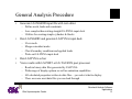
General Analysis Procedure
•
Generate LS-INGRID input file with text editor
– Define mesh, loads and constraints
– Less complex than writing straight LS-DYNA input deck
– Utilities for creating simple cylinders & blocks
•
Run LS-INGRID and generate LS-DYNA input deck
–
–
–
–
•
•
View mesh
Merge coincident nodes
Check boundary conditions and applied loads
Write out LS-DYNA input deck
Run LS-DYNA solver
View results with LS-POST or LS-TAURUS post processor
–
–
–
–
Reads in binary data files generated by LS-DYNA
Wide range of display options as well as animation capabilities
All calculated properties written to data files.....you select what to display
There are some ascii data files you can look through
2KLR6XSHUFRPSXWHU&HQWHU
6WUXFWXUDO$QDO\VLV6RIWZDUH
$SSOLFDWLRQV
15
Model Generation with LS-INGRID
7 fundamental concepts
–
–
–
–
–
–
–
Object space
Index space
Reduced index space
Index progression
Moving points, edges and planes
Boundary conditions
Defining and applying loads
The approach to building a complete model is to break it up into
rectangular or cubic blocks of nodes called regions. These regions can
then be combined to form the complete physical model.
2KLR6XSHUFRPSXWHU&HQWHU
6WUXFWXUDO$QDO\VLV6RIWZDUH
$SSOLFDWLRQV
16
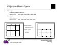
Object and Index Space
Object space
- Dimensions in physical space
- Specified as:
xmin, ymin, zmin, xmax, ymax, zmax
Index space
- Mesh attributes
- Specified as:
imin, jmin, kmin, imax, jmax, kmax
5
8
7
2EMHFWVSDFH
6
4
,QGH[VSDFH
3
2
J
5
Y
4
3
2
1
0
1
0
1
2
3
4
X
2KLR6XSHUFRPSXWHU&HQWHU
5
1
2
3
4
5
I
6WUXFWXUDO$QDO\VLV6RIWZDUH
$SSOLFDWLRQV
17
Index Progression
• Builds on the concept of an index region
imin jmin kmin imax jmax kmax
• This defines the “outside” dimensions of the region, but what if we
want to detail an internal component?
i.e. refine the mesh
• To change meshing in x-coordinate direction:
Index region
imin imax
xmin xmax
Index progression
imin i2 i3 i4 imax;jmin jmax; kmin kmax;
xmin x2 x3 x4 xmax ymin ymax zmin zmax
• Also gives the functionality to create multiple regions
• To set min=max, use a negative value
• A zero index is used to indicate that a structure is discontinuous
2KLR6XSHUFRPSXWHU&HQWHU
6WUXFWXUDO$QDO\VLV6RIWZDUH
$SSOLFDWLRQV
18
Reduced Index Space
• Forces and boundary conditions for the complete object are applied
when the region where the force is applied is defined
• Reduced index space means you are narrowing your focus to only the
index range of one particular part
• For a generic part
imin i1 i2 i3 imax;
We have reduced index # 1 2 3 4 5
2KLR6XSHUFRPSXWHU&HQWHU
6WUXFWXUDO$QDO\VLV6RIWZDUH
$SSOLFDWLRQV
19
Moving Regions
• mb <region> n dx dy dz
• <region> is defined using the reduced index
• n is a flag indicating which coordinate to change
x - x coordinate
xy - x and y coord.
y - y coordinate
xz - x and z coord.
z - z coordinate
yz - y and z coord.
xyz - x y and z coordinates are to be changed
• Only the coordinates required by flag n need be input.
• dx dy and dz are “added” to the existing x, y, z
2KLR6XSHUFRPSXWHU&HQWHU
6WUXFWXUDO$QDO\VLV6RIWZDUH
$SSOLFDWLRQV
20
Rotating Regions
•
•
rr <region> n theta;
<region> is defined using the reduced index
– n = rx rotate about the x axis
– n = ry rotate about the y axis
– n = rz rotate about the z axis
• theta is the angle in degrees that you wish to rotate
2KLR6XSHUFRPSXWHU&HQWHU
6WUXFWXUDO$QDO\VLV6RIWZDUH
$SSOLFDWLRQV
21
Boundary Conditions
• Objects we create on the computer are not infinite in size, they have
“boundaries” that define their size
• Setting the conditions at these boundaries is called applying boundary
conditions, or B.C.
• There are many types of B.C.
– displacement, pressure, temperature, velocity, etc.
• We are concerned with two types of B.C. or constraints for our
problem
– displacement (movement in the x,y or z direction)
– rotation (part will rotate about a given point)
2KLR6XSHUFRPSXWHU&HQWHU
6WUXFWXUDO$QDO\VLV6RIWZDUH
$SSOLFDWLRQV
22
Boundary Conditions
• The command is ‘b’ and it goes between the ‘start’ and ‘end’ of a part
description, but after the index and object space lines
• b <region> n
–
<region> is defined using the reduced index
• n is a 6 digit binary number
1st digit: x-displacement;
2nd digit: y-displacement
3rd digit: z-displacement
4th digit: x-rotation
5th digit: y-rotation
6th digit: z-rotation
2KLR6XSHUFRPSXWHU&HQWHU
=0 - free, =1 - fixed
6WUXFWXUDO$QDO\VLV6RIWZDUH
$SSOLFDWLRQV
23
Applied Loads
• There are 2 steps to applying a load
– Define the load curve
– Apply the load to a given part
• Load curve gives the magnitude of the force over time
• The load curve is ‘defined’ before the first part is defined
• Command
lcd
load#
npts
t1
force1
t2
force2 ...
where
load# is the load curve number
npts is the number of time/force data points
t1...tn are the time points
force1...forcen are the force values
2KLR6XSHUFRPSXWHU&HQWHU
6WUXFWXUDO$QDO\VLV6RIWZDUH
$SSOLFDWLRQV
24
Applying the Load Curve to a Part
• The load curve is applied between the ‘start’ and ‘end’ of a part
definition
• Command
fc
<region>
load#
mult
<direction>
where
<region> is defined using the reduced index
load# is the load curve number
mult is a multiplier (say if you want to double the force)
<direction> indicates which direction the force should act
format is xdir ydir zdir
•
1 0 0 would act in the positive x direction
0 -1 0 would act in the negative y direction
load curve can apply over an area or as a point load
2KLR6XSHUFRPSXWHU&HQWHU
6WUXFWXUDO$QDO\VLV6RIWZDUH
$SSOLFDWLRQV
25
Sample LS-INGRID Input File
Problem: Circular bar impacting
solid surface
bar impact problem (gm cm microsec)
dn3d
term 80.0
plti 1.0
prti 81.
velocity 0 0 -0.0227
c Define symmetry planes
plane 3 0 0 0 0 -1 0 .001 symm
0 0 0 -1 0 0 .001 symm
0 0 0 0 0 1 .001 symm
c Define bar
start
c Define index space
1 4 7 10 13;1 4 7 10 13;1 37;
c Define coordinate of index space
-.16 -.16 0 .16 .16 -.16 -.16 0 .16 .16 0 3.24
2KLR6XSHUFRPSXWHU&HQWHU
6WUXFWXUDO$QDO\VLV6RIWZDUH
$SSOLFDWLRQV
26
Sample LS-INGRID Input File
c Delete corners for cylindrical mapping
d 0 1 0 0 3 0
d 1 0 0 3 0 0
di 1 2 0 4 5;1 2 0 4 5;;
c Capture surfaces to be mapped
c and map in cyld. space
sfi -1 -5;-1 -5;;
cy 0 0 0 0 0 1 .32
mate 1
end
c Use tp 0.001 interactively in Ingrid
c Define material properties
mat 1 3
ro 8.93
sigy 0.004
e 1.17
etan 0.001
beta 1.0
pr 0.33
endmat
end end
2KLR6XSHUFRPSXWHU&HQWHU
6WUXFWXUDO$QDO\VLV6RIWZDUH
$SSOLFDWLRQV
27
Running LS-INGRID
Only available on Origin 2000
Command:
lsingrid
• When asked to choose display
device, select ‘X’ for X_Windows
• To load LS-INGRID input file:
Click on INPUT
Select INGRID File Type
Type in the name of your input file
Click on GRAPHICS
2KLR6XSHUFRPSXWHU&HQWHU
6WUXFWXUDO$QDO\VLV6RIWZDUH
$SSOLFDWLRQV
28
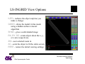
LS-INGRID View Options
IUPD - redraws the object anytime you
make a change
GOOD - draws the model in line mode
using a hidden surface removal
algorithm
SHAD - gives a solid shaded image
RX, RY, RZ - rotate object about the x, y,
or z axis respectively
ZIN - user selected zoom in
AC - scale the object to fit the entire screen
REST - restore the initial viewing settings
2KLR6XSHUFRPSXWHU&HQWHU
6WUXFWXUDO$QDO\VLV6RIWZDUH
$SSOLFDWLRQV
29
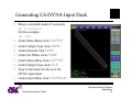
Generating LS-DYNA Input Deck
• Merge coincident nodes if necessary
tp tolerance
for this example
tp .001
• Under Main Menu click OUTPUT
• Under Output Type click DN3D
• Under Dyna3d click KW93
• Under Set Offset click DONE
• Under Main Menu click OUTPUT
• Under Output Type click FILE
• Type in the name for the new LSDYNA input deck
• Under main Menu click CONTINUE
2KLR6XSHUFRPSXWHU&HQWHU
6WUXFWXUDO$QDO\VLV6RIWZDUH
$SSOLFDWLRQV
30
Running LS-DYNA Solver on T90 & SV1
• LS-DYNA supported on all
platforms
• T90 & SV1 require the module
load command
• ja command provides a detailed
resource usage report including
maximum memory used
%DWFKVXEPLVVLRQILOH
#QSUB -r lsdyna_bar
#QSUB -lT 300
#QSUB -lM 16Mw
#QSUB -eo
set -x
module load lstc
cp $HOME/examples/lsdyna_bar/bar.dyna $TMPDIR
cd $TMPDIR
ja
lsdyna -v 950 I=bar.dyna O=bar.out
ja -clths
cp * $HOME/examples/lsdyna_bar
• Must specify a minimum of 16Mw
• Versions available
-v 940.1
(T90)
-v 940
(SV1)
-v 950
2KLR6XSHUFRPSXWHU&HQWHU
6WUXFWXUDO$QDO\VLV6RIWZDUH
$SSOLFDWLRQV
31
LS-DYNA Command Line Options
lsdyna I=inf o=otf G=ptf D=dpf F=thf T=tpf A=rrd M=sif J=jif
S=iff Z=isfl L=isf2 B=rlf W=root E=efl X=scl C=cpu K=kill
V=vda Y=c3d {KEYWORD} {THERMAL} {COUPLE} MEMORY=wds
The commonly used options are:
inf = input file (user specified)
otf = high speed printer file (default=D3HSP)
ptf = binary plot file for graphics (default=D3PLOT)
dpf = dump file for restarting (default=D3DUMP)
rrd = running restart dump file (default=RUNRSF)
sif = stress initialization file
nwds = number of words to be allocated
If you use the MEMORY command line option, you must request an additional 5Mw in your
batch script above what is given on the command line
2KLR6XSHUFRPSXWHU&HQWHU
6WUXFWXUDO$QDO\VLV6RIWZDUH
$SSOLFDWLRQV
32
Running LS-DYNA Solver on T3E
• T3E requires the module
load command
• ja command provides a detailed
resource usage report including
maximum memory used
• T3E jobs get full use of each
node assigned - therefore do not
specify any memory limit
%DWFKVXEPLVVLRQILOH
#QSUB -r lsdyna_pipe_8pe
#QSUB -l mpp_p=8
#QSUB -l mpp_t=700
#QSUB -eo
set -x
module add lstc
cp $HOME/examples/cylinder_8PE/pipe.dyna $TMPDIR
cd $TMPDIR
ja
mppdyna -np 8 I=pipe.dyna O=pipe.out
ja -clths
cp * $HOME/examples/lsdyna_cylinder_8PE
•LS-DYNA uses MPI on the T3E
• Note difference in command line
mppdyna -np <np> <executable> <options>
2KLR6XSHUFRPSXWHU&HQWHU
6WUXFWXUDO$QDO\VLV6RIWZDUH
$SSOLFDWLRQV
33
Running LS-DYNA Solver on T3E
Certain LS-DYNA runs may produce ASCII output files. They are first
produced as a series of files:
dbout.0001
dbout.0002
.
.
dbout.nnnn,
one for each CPU used in the analysis. To assemble the correct output,
first cat the dbout files and then process the result with dumpdbd
cat dbdout* > dbtotal
dumpdbd dbtotal
This will create the ASCII files: glstat, elout, nodout, etc. as specified in
the LS-DYNA input.
2KLR6XSHUFRPSXWHU&HQWHU
6WUXFWXUDO$QDO\VLV6RIWZDUH
$SSOLFDWLRQV
34
LS-DYNA Input Deck Parallel Modification
To run a parallel LS-DYNA job, you must modify the input deck
LS-DYNA3D Keyword file:
*CONTROL_PARALLEL
NCPU
NUMRHS ACCU
Variable
Description
NCPU
NUMRHS
Number of cpus used
Number of right-hand-sides written
0=same as NCPU (recommended for better parallel perf.)
1=write one only
Accuracy flag for parallel solution
1=on (default)
2=off, faster solution
ACCU
LS-DYNA3D Formatted file:
$ CARD 16: Computation Option -- Parallel and Subcycling
$...:....1....:....2....:....3....:....4....:....5....:....6....:....7....:....
$NCPU/SORT/SUBS/
24
2KLR6XSHUFRPSXWHU&HQWHU
6WUXFWXUDO$QDO\VLV6RIWZDUH
$SSOLFDWLRQV
35
Running LS-DYNA Solver on Origin 2000
• Origin does not requires the
module load command
• ssusage command provides
resource usage including maximum
memory used
• Must specify a minimum of
16Mw
• Modifications for parallel job
•Add “-l mpp_p=#“ specifier
• Add *CONTROL_PARALLEL
keyword line to dyna input deck
2KLR6XSHUFRPSXWHU&HQWHU
%DWFKVXEPLVVLRQILOHVHULDO
#QSUB -r lsdyna_bar
#QSUB -lT 300
#QSUB -lM 16Mw
#QSUB -eo
set -x
cp $HOME/examples/lsdyna_bar/bar.dyna $TMPDIR
cd $TMPDIR
ssusage lsdyna I=bar.dyna O=bar.out
cp * $HOME/examples/lsdyna_bar
%DWFKVXEPLVVLRQILOHSDUDOOHO
#QSUB -r lsdyna_bar
#QSUB -lT 300
#QSUB -lM 16Mw
#QSUB -l mpp_p=8
#QSUB -eo
set -x
cp $HOME/examples/lsdyna_bar/bar.dyna $TMPDIR
cd $TMPDIR
ssusage lsdyna I=bar.dyna O=bar.out
cp * $HOME/examples/lsdyna_bar
6WUXFWXUDO$QDO\VLV6RIWZDUH
$SSOLFDWLRQV
36
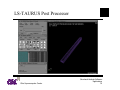
LS-TAURUS Post Processor
• Available on T90, SV1 and Origin
– Recommend running on Origin - better interactive response
– Avoid running on the T90 if possible - very limited memory
• There are two important command line options
ls-taurus_o g=ptf $
ptf = binary plot file (d3plot is the default)
$ allows 32 bit machine (i.e. Origin) read binary files written by 64 bit
machine (i.e. T90 and T3E)
• To run LS-TAURUS and read in the default data files
ls-taurus_o g=d3plot
• At startup you get 4 windows
–
–
–
–
Visualization Window
Phase 1 Menu
Viewbox
Commands & Messages
2KLR6XSHUFRPSXWHU&HQWHU
6WUXFWXUDO$QDO\VLV6RIWZDUH
$SSOLFDWLRQV
37
LS-TAURUS Post Processor
2KLR6XSHUFRPSXWHU&HQWHU
6WUXFWXUDO$QDO\VLV6RIWZDUH
$SSOLFDWLRQV
38
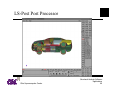
LS-Post Post Processor
• New post processor available from LS-DYNA
• Available on SV1 and Origin
– Recommend running on Origin - better interactive response
• There are two important command line options
ls-post
• At startup you get 1 window
– FILE -> OPEN
select these menus to read in the d3plot file
2KLR6XSHUFRPSXWHU&HQWHU
6WUXFWXUDO$QDO\VLV6RIWZDUH
$SSOLFDWLRQV
39
LS-Post Post Processor
2KLR6XSHUFRPSXWHU&HQWHU
6WUXFWXUDO$QDO\VLV6RIWZDUH
$SSOLFDWLRQV
40
LS-DYNA Web Information
LSTC web site
http://www.lstc.com
Official OSC supported software page
http://oscinfo.osc.edu/software
University of Cincinnati Center of Excellence in DYNA3D Analysis
http://www.ase.uc.edu/~atabiei/center.html
2KLR6XSHUFRPSXWHU&HQWHU
6WUXFWXUDO$QDO\VLV6RIWZDUH
$SSOLFDWLRQV
41
ABAQUS Package
ABAQUS Modeling Features
ABAQUS Components
ABAQUS Documentation
Generating ABAQUS Input File
Running ABAQUS Solver on Origin
Running ABAQUS Solver on T90
Viewing Results with ABAQUS/Post
Viewing Results with ABAQUS/Viewer
2KLR6XSHUFRPSXWHU&HQWHU
6WUXFWXUDO$QDO\VLV6RIWZDUH
$SSOLFDWLRQV
42
ABAQUS Modeling Features
ABAQUS/Standard is a general-purpose, production-oriented finite element
program. It provides a variety of time- and frequency-domain analysis
procedures. These procedures are divided into two classes: "general analyses,"
in which the response may be linear or nonlinear, and "linear perturbation
analyses," in which linear response is computed about a general, possibly
nonlinear, base state.
General Analyses
•Static stress/displacement analysis
•Viscoelastic/viscoplastic response
•Transient dynamic stress/displacement analysis
•Transient or steady-state heat transfer analysis
•Transient or steady-state mass diffusion analysis
•Thermo-mechanical (sequentially or fully coupled)
•Thermo-electrical
•Pore fluid flow-mechanical
•Stress-mass diffusion (sequentially coupled)
•Piezoelectric (linear only)
•Acoustic-mechanical (linear only)
2KLR6XSHUFRPSXWHU&HQWHU
Linear Perturbation Analyses
Static stress/displacement analysis:
Linear static stress/displacement analysis
Eigenvalue buckling load prediction
Dynamic stress/displacement analysis:
Determination of natural modes and frequencies
Transient response via modal superposition
Steady-state response resulting from harmonic loading
Response spectrum analysis
Dynamic response resulting from random loading
6WUXFWXUDO$QDO\VLV6RIWZDUH
$SSOLFDWLRQV
43
ABAQUS Modeling Features
ABAQUS/Explicit is designed specifically to serve advanced, nonlinear
continuum and structural analysis needs. The program addresses highly
nonlinear transient dynamic phenomena and certain nonlinear quasi-static
simulations. ABAQUS/Explicit uses explicit time integration for time stepping
and includes the following types of analyses:
•
•
•
Nonlinear dynamic stress/displacement analysis
Explicit dynamic response with or without adiabatic heating effects.
Annealing for multi-step forming simulations.
Material Definitions
• Elasticity:
Linear, hyperelasticity, viscoelasticity
• Plasticity and creep:
Metal plasticity, ductile failure, crushable foam, brittle cracking, brittle failure, strainrate-dependent plasticity and high-strain-rate failure
2KLR6XSHUFRPSXWHU&HQWHU
6WUXFWXUDO$QDO\VLV6RIWZDUH
$SSOLFDWLRQV
44
ABAQUS Components
9HUVLRQ
3UH3URFHVVRU$%$4863UH
$%$486&$(2ULJLQRQO\
3RVW3URFHVVRU$%$4863RVW
$%$4869LHZHU2ULJLQRQO\
6ROYHU$%$4866WDQGDUG
9HUVLRQ
$%$486([SOLFLW
2KLR6XSHUFRPSXWHU&HQWHU
6WUXFWXUDO$QDO\VLV6RIWZDUH
$SSOLFDWLRQV
45
ABAQUS Documentation
• Hardcopy Manuals are available for reading at OSC and can be
purchased from HKS, Inc.
• Online documentation is available on the Origin (v5.8 only)
ABAQUS Theory
ABAQUS Standard
Getting Started
Users Manual
Sample Problems
ABAQUS Explicit
Getting Started
Users Manual
Sample Problems
ABAQUS Viewer
ABAQUS CAE
2KLR6XSHUFRPSXWHU&HQWHU
(No online version)
(Volumes I, II, III)
(Volumes I, II)
(No online version)
(Volumes I, II)
6WUXFWXUDO$QDO\VLV6RIWZDUH
$SSOLFDWLRQV
46
General Analysis Procedure
• Generate ABAQUS input file with text editor
– Define mesh, loads and constraints
– Utilities for creating simple cylinders & blocks
• Run datacheck on input files
• View model with ABAQUS/Viewer
– View mesh
– Check boundary conditions and applied loads
• Run ABAQUS solver
• View results with ABAQUS post processor
– Wide range of display options as well as animation capabilities
NOTE: as of the spring 2000, ABAQUS/CAE is under evaluation and
only one license has been purchased
2KLR6XSHUFRPSXWHU&HQWHU
6WUXFWXUDO$QDO\VLV6RIWZDUH
$SSOLFDWLRQV
47
ABAQUS/Pre
Input file is split into two parts:
• Model data defines a finite element model
• History data defines what happens to the model
– User divides this history into a sequence of steps, each of which is a
period of response of a particular type (static loading, dynamic response,
etc.)
– Definition of a step includes
•
•
•
•
procedure type (static stress,transient heat transfer, etc.)
control parameters for time integration or for the nonlinear solution procedures
loading
output requests
2KLR6XSHUFRPSXWHU&HQWHU
6WUXFWXUDO$QDO\VLV6RIWZDUH
$SSOLFDWLRQV
48
ABAQUS/Pre
• All data definitions are accomplished with option blocks-sets of data
describing a part of the problem definition. Each option is introduced
by a keyword line.
• Keyword lines begin with a * in column 1, followed by the option
name
• ** is a comment
• Keyword lines are comma separated (free format)
• Data lines may be associated with the option; if so they must follow
the keyword line
2KLR6XSHUFRPSXWHU&HQWHU
6WUXFWXUDO$QDO\VLV6RIWZDUH
$SSOLFDWLRQV
49
ABAQUS/Pre - Model Data
• *NODE and *ELEMENT define individual entities
• *NGEN and *ELGEN generate a range of entities
• Nodes and elements can be grouped into sets
– NSET and ELSET keyword parameter (comma separated lists)
– Groups of elements or nodes can then be referred to as one entity
• Material definition (*MATERIAL)
– All keywords that follow the *MATERIAL option and introduce material
behavior relate to the given material until a keyword appears that does not
define material properties.
• Boundary conditions (*BOUNDARY)
– Degrees of freedom
• 1,2,3 - displacement components
• 4,5,6 - rotation components
• Other variables are available based on element type
2KLR6XSHUFRPSXWHU&HQWHU
6WUXFWXUDO$QDO\VLV6RIWZDUH
$SSOLFDWLRQV
50
ABAQUS/Pre - History Data
• History data is divided into steps
– *STEP option begins the step
– *END STEP closes the step
– Keyword optional parameter PERTURBATION
• *STATIC vs. *DYNAMIC
• Different types of loading
– *CLOAD concentrated load
– *DLOAD distributed load
– AMPLITUDE keyword option for time varying loads
2KLR6XSHUFRPSXWHU&HQWHU
6WUXFWXUDO$QDO\VLV6RIWZDUH
$SSOLFDWLRQV
51
ABAQUS/Pre - History Data
Results (.res) file
– Used by ABAQUS/Post for graphical post processing such as
deformed shape plots or contour plots
– Used to “restart” or continue an analysis
– Command to request that a restart file be written
*RESTART, WRITE, FREQUENCY=N, OVERLAY
– ABAQUS will write results to the restart file after each increment
at which the increment number is exactly divisible by N and at the
end of each step of the analysis
– OVERLAY parameter is used to specify that only one increment
should be retained on the restart file per step
2KLR6XSHUFRPSXWHU&HQWHU
6WUXFWXUDO$QDO\VLV6RIWZDUH
$SSOLFDWLRQV
52
ABAQUS/Pre - History Data
Object database (.odb) file
– Binary file used to store model information and analysis results for use by
ABAQUS/Viewer
– Variables to be written to the output database are defined by using the
following output variable identifiers
*OUTPUT, [FIELD|HISTORY], FREQUENCY
*ELEMENT OUTPUT, VARIABLE=ALL|PRESELECT
*NODE OUTPUT
*CONTACT OUTPUT
*ENERGY OUTPUT
– FIELD output is used to generate contour plots, displaced shape plots and
symbol plots (large data size, low sample frequency)
– HISTORY output is used to generate X-Y plots (small data size, high
sample frequency)
2KLR6XSHUFRPSXWHU&HQWHU
6WUXFWXUDO$QDO\VLV6RIWZDUH
$SSOLFDWLRQV
53
ABAQUS/Pre - History Data
Data (.dat) file
– Text file which contains information about the model definition and
tabular output of results.
– The values of output variables can be printed in tabular format throughout
the analysis.
*EL PRINT
*NODE PRINT
*CONTACT PRINT
*ENERGY PRINT
– Specify the variables to be printed in each output table
– For element variables, also specify the locations at which they are to be
printed
2KLR6XSHUFRPSXWHU&HQWHU
6WUXFWXUDO$QDO\VLV6RIWZDUH
$SSOLFDWLRQV
54
Sample ABAQUS Input File
*HEADING
SIMPLY SUPPORTED SQUARE PLATE WITH UNIFORM PRESSURE---S4R 4 X 4 MESH
*PREPRINT,ECHO=YES,MODEL=NO,HISTORY=NO
*RESTART, WRITE
*NODE, NSET=CORNERS
1,
0.,
0.
5,
1.,
0.
401, 0.,
1.
405, 1.,
1.
*NGEN,NSET=BOT
1,5,1
*NGEN,NSET=TOP
401,405,1
*NFILL
BOT,TOP,4,100
*NSET,NSET=SIDES,GENERATE
1,5,1
401,405,1
1,401,100
5,405,100
2KLR6XSHUFRPSXWHU&HQWHU
6WUXFWXUDO$QDO\VLV6RIWZDUH
$SSOLFDWLRQV
55
Sample ABAQUS Input File
*NSET,NSET=CENTND
203
*ELEMENT, TYPE=S4R
1, 1, 2, 102, 101
*ELGEN,ELSET=ALLELS
1,4,1,1,4,100,4
*ELSET,ELSET=CENTER
6,7,10,11
*MATERIAL ,NAME=METAL
*ELASTIC
3.E7, .3
*SHELL SECTION,MATERIAL=METAL,ELSET=ALLELS
.01,3
*BOUNDARY
SIDES,1,3
2KLR6XSHUFRPSXWHU&HQWHU
6WUXFWXUDO$QDO\VLV6RIWZDUH
$SSOLFDWLRQV
56
Sample ABAQUS Input File
*STEP
*STATIC
*DLOAD
ALLELS,P,-1.
*NODE PRINT, NSET=CENTND
U
*EL PRINT, ELSET=CENTER, POSITION=AVERAGED AT NODES
SF
*NODE FILE, NSET=CENTND
U
*EL FILE, ELSET=CENTER, POSITION=AVERAGED AT NODES
SF
*END STEP
2KLR6XSHUFRPSXWHU&HQWHU
6WUXFWXUDO$QDO\VLV6RIWZDUH
$SSOLFDWLRQV
57
Running ABAQUS Solver on Origin 2000
abaqus -v[5.7|5.8-1|5.8-17] interactive [viewer|post|datacheck] job=jobid
where jobid =name of input file without extension
Required:
– interactive keyword
– Job name
Strongly suggested:
– Code version desired
2KLR6XSHUFRPSXWHU&HQWHU
%DWFKVXEPLVVLRQILOH
#QSUB -r s4r_4x4
#QSUB -lM 16Mw
#QSUB -lT 1:00:00
#QSUB -eo
set -x
cp ~jimg/examples/abaqus/s4r_4x4/s4r_4x4.inp $TMPDIR
cd $TMPDIR
ssusage abaqus -v5.8-17 interactive job=s4r_4x4
cp * ~jimg/examples/abaqus/s4r_4x4
6WUXFWXUDO$QDO\VLV6RIWZDUH
$SSOLFDWLRQV
58
Running datacheck Prior to Solver
[origin]$ abaqus -v5.8-1 datacheck interactive job=s4r_4x4
ABAQUS JOB s4r_4x4
BEGIN USER INPUT PROCESSING
Wed May 19 00:55:16 EDT 1999
Run /local/abaqus/5.8/bin/pre.x
ABAQUS License Server checked out 5 Network Tokens
Wed May 19 00:55:19 EDT 1999
END OF USER INPUT PROCESSING
BEGIN IMPLICIT DATACHECK
Wed May 19 00:55:19 EDT 1999
Run /local/abaqus/5.8/bin/standard.x
ABAQUS License Server checked out 5 Network Tokens
Wed May 19 00:55:21 EDT 1999
END OF DATACHECK
ABAQUS JOB s4r_4x4 COMPLETED
-rw-r--r--rwxr-----rw-r--r--rw-r--r--rw-r-----rw-r--r--rw-r--r--rw-r--r--rw-r-----
2KLR6XSHUFRPSXWHU&HQWHU
5HVXOWLQJ'DWD)LOHV
1
1
1
1
1
1
1
1
1
57456
2392
11789
4104
795
1186
62968
98304
49524
May
May
May
May
May
May
May
May
May
19
19
19
19
19
19
19
19
19
00:55
00:55
00:55
00:55
00:53
00:55
00:55
00:55
00:55
s4r_4x4.023
s4r_4x4.com
s4r_4x4.dat
s4r_4x4.fil
s4r_4x4.inp
s4r_4x4.msg
s4r_4x4.odb
s4r_4x4.res
s4r_4x4.sdb
6WUXFWXUDO$QDO\VLV6RIWZDUH
$SSOLFDWLRQV
59
Running ABAQUS Solver on T90
[OSCA]$ abaqus -v5.7 job=s4r_4x4
ACADEMIC ABAQUS 5.7-1 Network --- CRAY
JOB TIME LIMIT ?
enter s for s secs.
enter m:s for m mins., s secs.
enter h:m:s for hrs, mins., secs.
or carriage return for 1:0
: 120
enter m for m megawords or
carriage return for 8 Mw : 8
ABAQUS/STANDARD is running on a Category D machine.
nqs-181 qsub: INFO
Request <7567.osca>: Submitted to queue <batch> by <jimg(6815)>.
5HVXOWLQJ'DWD)LOHV
-rw-r--r--rwxr-----rw-r--r--rw-r-----rw-r--r--rw-r--r--rw-r--r--
2KLR6XSHUFRPSXWHU&HQWHU
1
1
1
1
1
1
1
0
2393
2363
795
4960
2854
70
May
May
May
May
May
May
May
19
19
19
19
19
19
19
02:07
02:07
02:07
01:50
02:07
02:07
02:07
abaqus.env
s4r_4x4.com
s4r_4x4.dat
s4r_4x4.inp
s4r_4x4.log
s4r_4x4.msg
s4r_4x4.q
6WUXFWXUDO$QDO\VLV6RIWZDUH
$SSOLFDWLRQV
60
Viewing Results with ABAQUS/Post
•
•
•
ABAQUS/Post is being replaced by ABAQUS/Viewer
Text command interface
Mouse input for image rotation, displacement and zoom
abaqus -v5.8 post restart=s4r_4x4
Reading restart file : s4r_4x4
ABAQUS Version: 5.8-1
No.
No.
No.
No.
Reading
Reading
Reading
Reading
of
of
of
of
elements
nodes
element sets
node sets
:
:
:
:
Date: 12-MAY-1999
16
25
3
6
element data...
node data...
element sets...
node sets...
Restart file = s4r_4x4
Current step/inc = 1 / 1
2KLR6XSHUFRPSXWHU&HQWHU
6WUXFWXUDO$QDO\VLV6RIWZDUH
$SSOLFDWLRQV
61
ABAQUS/Post Commands
draw, options
displaced - original grid and deformed grid overlaid in different colors
contour, options
variable=parameter (required) - name of the variable to be contoured
range - print the min and max values of this variable, without plotting
set, options
underformed=[on|off] - command to plot only the deformed shape
d magnification=# - scale displacements to improve display
n numbers=[on|off] - option to display node numbers
el numbers=[on|off] - option to display element numbers
nodes=# - control the size of dot symbol displayed at node locations
bc display=[on|off] - toggles the plotting of boundary conditions
load display=[on|off] - toggles the plotting of loads
fill=[on|off] - contour plots with discrete filled colored regions
shade=[on|off] - contour plots with smooth shaded colored regions
2KLR6XSHUFRPSXWHU&HQWHU
6WUXFWXUDO$QDO\VLV6RIWZDUH
$SSOLFDWLRQV
62
ABAQUS/Post Commands
report elements, parameter
Report the element number, element type, material name (if applicable) and nodal connectivity list
displaced - this parameter indicates the displaced shape is to be used to select the elements for
reporting
report nodes, parameter
Report the node number, the current coordinates, and, if available, the displacements for nodes
picked
displaced - see description above
original - use this parameter if the reported coordinates will be those of the undeformed shape
report values, parameter
variable=name(required) - name of the variable to be reported
displaced - see description above
integration point - set this parameter equal to the element integration point at which the
variable is to be obtained; default is all integration points
2KLR6XSHUFRPSXWHU&HQWHU
6WUXFWXUDO$QDO\VLV6RIWZDUH
$SSOLFDWLRQV
63
ABAQUS/Post Example Problem
2KLR6XSHUFRPSXWHU&HQWHU
6WUXFWXUDO$QDO\VLV6RIWZDUH
$SSOLFDWLRQV
64
Viewing Results with ABAQUS/Viewer
•
•
•
All of the functionality of
ABAQUS/Post with nice GUI
interface
Will replace ABAQUS/Post after v5.8
What “replace” actually means is yet
to be determined
abaqus -v5810 viewer odb=jobname
2KLR6XSHUFRPSXWHU&HQWHU
6WUXFWXUDO$QDO\VLV6RIWZDUH
$SSOLFDWLRQV
65
ABAQUS Web Information
• ABAQUS Home page:
http://www.abaqus.com
• ABAQUS Examples:
http://www.abaqus.com/applications/applications.html
• ABAQUS Training:
http://www.abaqus.com/training-services/training-services.html
• Official OSC supported software page:
http://oscinfo.osc.edu/software
2KLR6XSHUFRPSXWHU&HQWHU
6WUXFWXUDO$QDO\VLV6RIWZDUH
$SSOLFDWLRQV
66
ANSYS Package
ANSYS Modeling Features
ANSYS Components
ANSYS Documentation
Model Development
Running ANSYS Solver on T90
Running ANSYS Solver on Origin
ANSYS Post Processing
2KLR6XSHUFRPSXWHU&HQWHU
6WUXFWXUDO$QDO\VLV6RIWZDUH
$SSOLFDWLRQV
67
ANSYS Modeling Features
Nonlinear and linear analysis
Structural
–
static, dynamic, buckling, kinematic
Thermal
–
steady-state, transient, phase change, radiation
Acoustics
Coupled field
–
–
–
–
Thermal-structural
Acoustics-structural
Thermal-electric
Piezoelectrics
Materials
–
–
–
–
–
–
–
Elements
–
–
–
–
–
–
–
–
2KLR6XSHUFRPSXWHU&HQWHU
Plasticity
Hyperelasticity
Viscoplasticity
Viscoelasticity
Creep, swelling
Temperature-dependent properties
Phase change via enthalpy
Quadrilateral, triangle, mixed quad/triangle,
mapped brick and tetrahedral
Cables and compression only spars
Surface-to-surface contact w/friction
Node-to-node contact with friction
Cracking and/or crushing solids
Element birth and death
Substructuring for linear regions
Thermal-electric shell
6WUXFWXUDO$QDO\VLV6RIWZDUH
$SSOLFDWLRQV
68
ANSYS Components
•
•
Solver, Pre and Post processor are integrated into one package
Preprocessor
–
–
–
–
–
–
•
Motif-based windows look and feel
Cascading pull-down menus
Online-documentation and hyper-text-linked help
Automatic FE mesh generation
Adaptive, mapped meshing
P- and h- element meshing
Postprocessing
– Contours, vector displays and graphics of potentials and field data
– Animation of results data
– 3D volume visualization tools including isosurfaces, gradient displays, volume
slicing, section displays and translucency
– General line integral and mapping features
2KLR6XSHUFRPSXWHU&HQWHU
6WUXFWXUDO$QDO\VLV6RIWZDUH
$SSOLFDWLRQV
69
ANSYS Documentation
• Hardcopy manuals can be purchased from HKS, Inc.
• Full on-line documentation is available:
module load ansys
anshelp55
ANSYS Basic Analysis Procedures Guide
ANSYS Modeling and Meshing Guide
ANSYS Structural Analysis Guide
ANSYS Thermal Analysis Guide
ANSYS Coupled-Field Analysis Guide
ANSYS Advanced Analysis Techniques
ANSYS Commands Manual
ANSYS Elements Manual
ANSYS Theory Manual
ANSYS Operations Guide
• Hypertext-based help system is also available via “HELP” buttons
during the analysis
2KLR6XSHUFRPSXWHU&HQWHU
6WUXFWXUDO$QDO\VLV6RIWZDUH
$SSOLFDWLRQV
70
General Analysis Procedure
Assemble model - graphical interface
•
•
•
•
•
•
•
Select element types and set options
Define real constants
Define material properties
Generate model geometry
Mesh geometry
Apply boundary conditions
Apply loads
Run solver - batch mode
View results - graphical interface
•
•
•
Deformed shape plot
Contour plots
X-Y data plots
2KLR6XSHUFRPSXWHU&HQWHU
6WUXFWXUDO$QDO\VLV6RIWZDUH
$SSOLFDWLRQV
71
ANSYS Command Line Options
ansys -m MW -j jobname -g
-m MW: This option specifies the amount of working storage obtained from
the system. The units are megawords. The memory requirement for the
entire execution will be approximately 5.3 megawords more than the -m
specification.
-j jobname: This option allows the user to specify the jobname on the
command line. When loading data, ANSYS uses the jobname as the file
name and looks for specific extensions.
-g: Specifies that the ANSYS menu system be started automatically.
ANSYS requires the module load command to set proper environment
variables
module load ansys
2KLR6XSHUFRPSXWHU&HQWHU
6WUXFWXUDO$QDO\VLV6RIWZDUH
$SSOLFDWLRQV
72
ANSYS User Interface
Main Menu
•Primary ANSYS functions
•Pop-up menus based on the progression
of the program
Utility Menu
•Pull-down menus
•Available any time during analysis
Input Window
•Provides area for typing in ANSYS
commands
•Command history
Graphics Window
•Area for graphics display
Toolbar
•One-click access to common functions
•User can customize the toolbar
2KLR6XSHUFRPSXWHU&HQWHU
6WUXFWXUDO$QDO\VLV6RIWZDUH
$SSOLFDWLRQV
73
Model Development
Preprocessor
•ANSYS Main Menu will be the starting point for each
phase of the analysis
•Preferences allow you to specify what type of
analysis you are performing
•This will mask out unwanted menu items
•“Preprocessor” selection brings up the menu on the
right
2KLR6XSHUFRPSXWHU&HQWHU
6WUXFWXUDO$QDO\VLV6RIWZDUH
$SSOLFDWLRQV
74
Selecting Elements in ANSYS
• Elements are first added to the “active” list
• Material and other physical properties are assigned
• During the meshing procedure, “active” elements can be selected
Choosing ELEMENT TYPE from the preprocessor
window allows you select the element(s) you want to add
Once an element is added, you
must also define OPTIONS for the
particular element type
2KLR6XSHUFRPSXWHU&HQWHU
6WUXFWXUDO$QDO\VLV6RIWZDUH
$SSOLFDWLRQV
75
Defining Real Constants
ADD
OK
•Elements often have properties not defined by node locations
•Only elements added in the previous step will appear in the Real
Constants window
•HELP button in last window gives very detailed information about
the element selected. This is an excellent source of information.
2KLR6XSHUFRPSXWHU&HQWHU
6WUXFWXUDO$QDO\VLV6RIWZDUH
$SSOLFDWLRQV
76
Material Properties
Isotropic
OK
•Material properties may be linear, nonlinear and/or
anisotropic
•Material properties are independent of geometry
•Multiple material property sets may be defined
•Select LIST to see what material property sets have been
previously defined
2KLR6XSHUFRPSXWHU&HQWHU
6WUXFWXUDO$QDO\VLV6RIWZDUH
$SSOLFDWLRQV
77
Creating Model Geometry
•ANSYS interface has many CAD features
•General procedure
•Build up basic model with circles, rectangles
•Create more complex areas with lines and splines
•Refine model with rounding and fillets
•Subtract, combine and/or add areas
•You can create points, lines, areas and volumes
Create
2KLR6XSHUFRPSXWHU&HQWHU
6WUXFWXUDO$QDO\VLV6RIWZDUH
$SSOLFDWLRQV
78
Modeling Operate Functions
•Powerful features that allow you to create complex geometry
from simpler objects
•Intersect generates an area from the overlapping parts of two
areas
•Add combines multiple areas into one
•Subtract allows you to create voids in a solid area
2KLR6XSHUFRPSXWHU&HQWHU
6WUXFWXUDO$QDO\VLV6RIWZDUH
$SSOLFDWLRQV
79
Corner Bracket Example
2KLR6XSHUFRPSXWHU&HQWHU
6WUXFWXUDO$QDO\VLV6RIWZDUH
$SSOLFDWLRQV
80
Corner Bracket Example
2KLR6XSHUFRPSXWHU&HQWHU
6WUXFWXUDO$QDO\VLV6RIWZDUH
$SSOLFDWLRQV
81
Corner Bracket Example
2KLR6XSHUFRPSXWHU&HQWHU
6WUXFWXUDO$QDO\VLV6RIWZDUH
$SSOLFDWLRQV
82
Meshing
Mesher Options
•Use automatic meshing for first cut
•Refine using MeshTool if needed
•Suggest turning on Accept/Reject prompt
•Use Size Controls option to control size of
elements in initial mesh
OK
2KLR6XSHUFRPSXWHU&HQWHU
6WUXFWXUDO$QDO\VLV6RIWZDUH
$SSOLFDWLRQV
83
Loads and Boundary Conditions
Apply
Displacement
KEXPND (expand displacements) allows the displacement constraint to
be applied not only to the nodes that correspond to the picked keypoints,
but to all nodes between the keypoints as well
2KLR6XSHUFRPSXWHU&HQWHU
6WUXFWXUDO$QDO\VLV6RIWZDUH
$SSOLFDWLRQV
84
Loads and Boundary Conditions
Pressure
On Lines
By various options, pick the line
you want to apply the pressure
load to
•Entering different values for VALI and VALJ
will apply a linear pressure load between the
endpoints of the line
•Pressure is always positive into the
material
2KLR6XSHUFRPSXWHU&HQWHU
6WUXFWXUDO$QDO\VLV6RIWZDUH
$SSOLFDWLRQV
85
Loads and Boundary Conditions
2KLR6XSHUFRPSXWHU&HQWHU
6WUXFWXUDO$QDO\VLV6RIWZDUH
$SSOLFDWLRQV
86
Running ANSYS Solver on T90
%DWFKVXEPLVVLRQILOH
• Environment variables set up
with the module load
command
• ja command provides a detailed
resource usage report including
maximum memory used
• Must specify a minimum of
17Mw
• commands.txt file contains
the actual commands that are sent
to the ANSYS program
2KLR6XSHUFRPSXWHU&HQWHU
#QSUB -r ansys
#QSUB -lT 300
#QSUB -lM 20Mw
#QSUB -eo
set -x
module load ansys
cp $HOME/examples/ansys/* $TMPDIR
ja
ansys -j bracket < commands.txt
ja -cst
cp * $HOME/examples/ansys
FRPPDQGVW[W
RESUME
/SOLU
CHECK
SOLVE
FINISH
/EXIT,ALL
6WUXFWXUDO$QDO\VLV6RIWZDUH
$SSOLFDWLRQV
87
Running ANSYS Solver on Origin
%DWFKVXEPLVVLRQILOH
• Environment variables set up
with the module load
command
• ssusage command provides
resource usage report including
maximum memory used
• commands.txt file contains
the actual commands that are sent
to the ANSYS program
2KLR6XSHUFRPSXWHU&HQWHU
#QSUB -r ansys
#QSUB -lT 300
#QSUB -lM 20Mw
#QSUB -eo
set -x
module load ansys
cp $HOME/examples/ansys/* $TMPDIR
ssusage ansys -j bracket < commands.txt
cp * $HOME/examples/ansys
FRPPDQGVW[W
RESUME
/SOLU
CHECK
SOLVE
FINISH
/EXIT,ALL
6WUXFWXUDO$QDO\VLV6RIWZDUH
$SSOLFDWLRQV
88
ANSYS Postprocessing
• After batch job completes, review log file for errors
• Restart ANSYS in graphical interface mode with the correct job name
ansys -g -j bracket
• From the TOOLBAR, click RESUME_DB
or
From the UTILITY MENU, click RESUME JOBNAME.DB from the
FILE pull down menu
2KLR6XSHUFRPSXWHU&HQWHU
6WUXFWXUDO$QDO\VLV6RIWZDUH
$SSOLFDWLRQV
89
ANSYS Postprocessing
•After solution is obtained, you must read in the results by
selecting one of the options under READ RESULTS
•Results fall into 4 major categories
•Deformed shape plots
Plot Results
•Contour plots
•X-Y plots
•Viewing numerical results
Deformed Shape
2KLR6XSHUFRPSXWHU&HQWHU
6WUXFWXUDO$QDO\VLV6RIWZDUH
$SSOLFDWLRQV
90
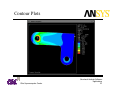
Contour Plots
•Contours available for both nodal and element properties
•All parameters saved, no need to specify before the solution
which parameters you would like to examine
Nodal Soln
2KLR6XSHUFRPSXWHU&HQWHU
6WUXFWXUDO$QDO\VLV6RIWZDUH
$SSOLFDWLRQV
91
Contour Plots
2KLR6XSHUFRPSXWHU&HQWHU
6WUXFWXUDO$QDO\VLV6RIWZDUH
$SSOLFDWLRQV
92
Viewing Numerical Results
•Procedure similar to contour plots
•Rather than a plot appearing, a text window
will pop up with tabulated data within
List Results
2KLR6XSHUFRPSXWHU&HQWHU
6WUXFWXUDO$QDO\VLV6RIWZDUH
$SSOLFDWLRQV
93
ANSYS Web Information
• ANSYS home page:
http://www.ansys.com
• List of ANSYS documentation:
http://www.ansys.com/ServSupp/Library/library.html
• Vendor training:
http://www.ansys.com/ServSupp/Training/index.html
• "ANALYSIS SOLUTIONS", an independent magazine covering
design analysis and optimization for ANSYS users:
http://www.analysismag.com
• Downloadable information:
http://www.ansys.com/Download
• Official OSC supported software page:
http://oscinfo.osc.edu/software
2KLR6XSHUFRPSXWHU&HQWHU
6WUXFWXUDO$QDO\VLV6RIWZDUH
$SSOLFDWLRQV
94