Download A+CAL User`s Manual - Microsoft Research

A +CAL User’s Manual
Leslie Lamport
27 Dec 2005
Contents
Preface
1
1 Introduction
2
2 Getting Started
2.1 Typing the Algorithm . .
2.2 The TLA+ Module . . . .
2.3 Translating and Executing
2.4 Checking the Results . . .
2.5 Checking Termination . .
2.6 A Multiprocess Algorithm
.
.
.
.
.
.
.
.
.
.
.
.
.
.
.
.
.
.
.
.
.
.
.
.
.
.
.
.
.
.
.
.
.
.
.
.
.
.
.
.
.
.
.
.
.
.
.
.
.
.
.
.
.
.
4
4
6
7
9
9
10
3 The Language
3.1 Expressions . . . . . . . . . . . .
3.2 The Statements . . . . . . . . . .
3.2.1 Assignment . . . . . . . .
3.2.2 If . . . . . . . . . . . . . .
3.2.3 Either . . . . . . . . . . .
3.2.4 While . . . . . . . . . . .
3.2.5 When . . . . . . . . . . .
3.2.6 With . . . . . . . . . . . .
3.2.7 Skip . . . . . . . . . . . .
3.2.8 Print . . . . . . . . . . . .
3.2.9 Assert . . . . . . . . . . .
3.2.10 Call and Return . . . . .
3.2.11 Goto . . . . . . . . . . . .
3.3 Processes . . . . . . . . . . . . .
3.4 Procedures . . . . . . . . . . . .
3.5 Macros . . . . . . . . . . . . . . .
3.6 Definitions . . . . . . . . . . . . .
3.7 Labels . . . . . . . . . . . . . . .
3.8 The Translation’s Definitions and
. . . . . . . .
. . . . . . . .
. . . . . . . .
. . . . . . . .
. . . . . . . .
. . . . . . . .
. . . . . . . .
. . . . . . . .
. . . . . . . .
. . . . . . . .
. . . . . . . .
. . . . . . . .
. . . . . . . .
. . . . . . . .
. . . . . . . .
. . . . . . . .
. . . . . . . .
. . . . . . . .
Declarations
.
.
.
.
.
.
.
.
.
.
.
.
.
.
.
.
.
.
.
.
.
.
.
.
.
.
.
.
.
.
.
.
.
.
.
.
.
.
.
.
.
.
.
.
.
.
.
.
.
.
.
.
.
.
.
.
.
.
.
.
.
.
.
.
.
.
.
.
.
.
.
.
.
.
.
.
.
.
.
.
.
.
.
.
.
.
.
.
.
.
.
.
.
.
.
.
.
.
.
.
.
.
.
.
.
.
.
.
.
.
.
.
.
.
.
.
.
.
.
.
.
.
.
.
.
.
.
.
.
.
.
.
.
.
.
.
.
.
.
.
.
.
.
.
.
.
.
.
.
.
.
.
16
17
17
17
18
19
20
20
20
21
21
21
22
22
22
23
25
26
26
27
4 Checking the Algorithm
4.1 Running the Translator . . .
4.2 Specifying the Constants . . .
4.3 Constraints . . . . . . . . . .
4.4 Understanding TLC’s Output
.
.
.
.
.
.
.
.
.
.
.
.
.
.
.
.
.
.
.
.
.
.
.
.
.
.
.
.
.
.
.
.
.
.
.
.
30
30
31
33
33
. . . . . . . . .
. . . . . . . . .
the Algorithm
. . . . . . . . .
. . . . . . . . .
. . . . . . . . .
.
.
.
.
.
.
.
.
.
.
.
.
.
.
.
.
.
.
.
.
.
.
.
.
.
.
.
.
.
.
.
.
.
.
.
.
.
.
.
.
.
.
.
.
.
.
.
.
4.5
4.6
4.7
Invariance Checking . . .
Termination and Liveness
Additional TLC Features
4.7.1 Deadlock Checking
4.7.2 Multithreading . .
4.7.3 Symmetry . . . . .
.
.
.
.
.
.
.
.
.
.
.
.
.
.
.
.
.
.
.
.
.
.
.
.
.
.
.
.
.
.
.
.
.
.
.
.
.
.
.
.
.
.
.
.
.
.
.
.
.
.
.
.
.
.
.
.
.
.
.
.
.
.
.
.
.
.
.
.
.
.
.
.
.
.
.
.
.
.
.
.
.
.
.
.
.
.
.
.
.
.
.
.
.
.
.
.
.
.
.
.
.
.
.
.
.
.
.
.
.
.
.
.
.
.
.
.
.
.
.
.
35
35
38
38
39
39
5 TLA+ Expressions and Definitions
5.1 Numbers . . . . . . . . . . . . . . . . . . . . .
5.2 Strings . . . . . . . . . . . . . . . . . . . . . .
5.3 Boolean Operators . . . . . . . . . . . . . . .
5.4 Sets . . . . . . . . . . . . . . . . . . . . . . .
5.5 Functions . . . . . . . . . . . . . . . . . . . .
5.6 Records . . . . . . . . . . . . . . . . . . . . .
5.7 The Except Construct . . . . . . . . . . . . .
5.8 Tuples and Sequences . . . . . . . . . . . . .
5.9 Miscellaneous Constructs . . . . . . . . . . .
5.10 Temporal Operators . . . . . . . . . . . . . .
5.10.1 Fairness . . . . . . . . . . . . . . . . .
5.10.2 Liveness . . . . . . . . . . . . . . . . .
5.10.3 One Algorithm Implementing Another
5.11 TLA+ Definitions . . . . . . . . . . . . . . . .
.
.
.
.
.
.
.
.
.
.
.
.
.
.
.
.
.
.
.
.
.
.
.
.
.
.
.
.
.
.
.
.
.
.
.
.
.
.
.
.
.
.
.
.
.
.
.
.
.
.
.
.
.
.
.
.
.
.
.
.
.
.
.
.
.
.
.
.
.
.
.
.
.
.
.
.
.
.
.
.
.
.
.
.
.
.
.
.
.
.
.
.
.
.
.
.
.
.
.
.
.
.
.
.
.
.
.
.
.
.
.
.
.
.
.
.
.
.
.
.
.
.
.
.
.
.
41
41
41
42
43
45
46
46
47
48
49
49
51
52
52
References
53
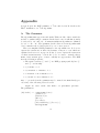
A The Grammar
54
B The TLA+ Translation
57
B.1 The FastMutex Algorithm . . . . . . . . . . . . . . . . . . . . 57
B.2 Procedures . . . . . . . . . . . . . . . . . . . . . . . . . . . . 61
Index
66
Preface
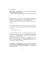
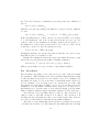
This is an instruction manual for the +cal algorithm language. Section 1
explains what an algorithm language is and why you’d want to use one.
Section 2 tells you what you need to know to get started using +cal. After
reading it, you’ll be able to write and check +cal algorithms.
You can read the other parts of this manual as you need them. The table
of contents and the index can help you find what you need. Pages 63–65 at
the end, just before the index, contain a series of tables that summarize a
lot of useful information. The rest of the manual is arranged in the order
you’re likely to want to look at it:
• Section 3 describes the things you’ll find in most programming language manuals, like the statements of the language. Once you’ve
started writing +cal algorithms, you should browse this chapter to
learn about features of +cal not mentioned in Section 2.
• We run programs, but we check algorithms. Section 2 gets you started
using the translator and TLC model checker to check +cal algorithms.
Section 4 tells you more about the translator and TLC. It’s mostly
about TLC, describing some of its additional features and how to use
it to debug an algorithm. You should go to Section 4 if you don’t
understand what the translator or TLC is trying to say when it reports
an error.
• Section 5 is mainly about writing +cal expressions. The expression
language of +cal is much richer and more powerful than that of any
programming language because it is based on mathematics, not on
programming. The ten or so pages about expressions in Section 5 just
introduce the subject. You can learn more from the book Specifying
Systems, referred to here as the TLA+ book [2], or from any books on
the elementary mathematics of sets, functions, and logic—especially
ones written by mathematicians and not computer scientists.
• Section A of the appendix contains a BNF grammar of +cal. The
subject of Appendix Section B will make no sense to you until you’ve
read Section 1.
I wish to thank the people who helped make +cal possible. Keith Marzullo
collaborated in the writing of the translator and helped with the design of
the +cal language. Georges Gonthier made many useful suggestions for the
language.
1
1
Introduction
+cal
(pronounced “plus-CAL”) is an algorithm language. An algorithm
language is meant for writing algorithms, not programs. Algorithms differ
from programs in several ways:
• Algorithms perform operations on arbitrary mathematical objects,
such as graphs and vector spaces. Programs perform operations on
simple objects such as Booleans and integers; operations on more complex data types must be coded using lower-level operations such as
integer addition and method invocation.
• A program describes one method of computing a result; an algorithm
may describe a class of possible computations. For example, an algorithm might simply require that a certain operation be performed for
all values of i from 1 to N . A program specifies in which order those
operations are performed.
• Execution of an algorithm consists of a sequence of steps. An algorithm’s computational complexity is the number of steps it takes to
compute the result; defining a concurrent algorithm requires specifying what constitutes a single (atomic) step. There is no well-defined
notion of a step of a program.
These differences between algorithms and programs are reflected in the following differences between +cal and programming languages.
• The language of +cal expressions is TLA+, a high-level specification
language based on set theory and first-order logic [2]. TLA+ is infinitely more expressive than the expression language of any programming language. Even the subset of TLA+ that can be executed by
the TLC model checker is far more expressive than any programming
language.1
•
+cal
•
+cal
provides simple constructs for expressing nondeterminism.
uses labels to describe the algorithm’s steps. This works quite
well for describing the grain of atomicity in the absence of procedure
calls. Invoking a procedure and returning from a procedure must begin
1
SETL [3] provides many of the set-theoretic primitives of TLA+, but it can implement higher-level operations only by programming them with procedures and it cannot
conveniently express nondeterminism.
2
new steps, which does limit the flexibility of describing atomicity in
algorithms with procedures. However, +cal’s macro facility and the
ability to define operators in TLA+ and use them in +cal expressions
often make procedure calls unnecessary.
The primary goals of a programming language are efficiency of execution
and ease of writing large programs. The primary goals of an algorithm
language are making algorithms easier to understand and helping to check
their correctness. Efficiency matters when executing a program that implements the algorithm. Algorithms are much shorter than programs, typically
dozens of lines rather than thousands. An algorithm language doesn’t need
complicated concepts like objects or sophisticated type systems that were
developed for writing large programs.
It is easy to write a +cal algorithm that cannot be executed—for example, one containing a statement that assigns to x the smallest integer
for which Goldbach’s conjecture2 is false, if one exists, or else the value 0.
An unexecutable algorithm can be interesting, and may represent a step in
the development of a practical algorithm. However, most +cal users will
want to execute their algorithms. The +cal translator compiles a +cal
algorithm into a TLA+ specification. If the algorithm manipulates only finite objects in a sensible way, then the TLC model checker will probably
be able to execute that specification. When used in model-checking mode,
TLC will check all possible executions of the algorithm. It can also be used
in simulation mode to check randomly generated executions.
2
Goldbach’s conjecture, which has not been proved or disproved, asserts that any even
number greater than 2 is the sum of two primes.
3
2
Getting Started
I assume here that you’ve programmed in an imperative language like Java or
Pascal or C. I will therefore not bother to explain the meaning of something
like a while statement that appears in such languages. You can find the
meaning of while and all other +cal statements in Section 3. (The index
can help you.)
2.1
Typing the Algorithm
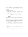
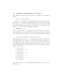
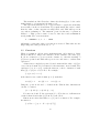
As an example, consider the following bit of +cal code that describes
Euclid’s algorithm, adapted from a version given by Sedgewick [4, page
8]. It sets v to the gcd (greatest common divisor) of u and v.
lp: while u 6= 0 do (∗ 6= is typed # or /= or \neq . ∗)
if u < v then u := v || v := u ; \∗ swap u and v.
end if ;
a: u := u - v;
end while ;
Comments indicate how to type symbols such as “ 6= ” that appear in the
examples. A complete list of the ascii versions of symbols appears in Table 5
on page 65.
You should find this code easy to understand, except for the “||” in the
then clause on the second line. Assignment statements separated by “||”s
(rather than by semicolons) are executed simultaneously by first evaluating
all the right-hand sides, then doing the assignments. Thus, as the comment
says, that multiple assignment swaps the values of u and v.
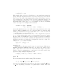
Also unusual in this piece of code is the presence of the labels lp and
a. They serve to delimit the steps of the algorithm. A step consists of the
execution from one label to the next. One iteration of the while loop, when
u is nonzero, consists of two steps:
• The step from lp to a, which executes the test u 6= 0 and the if
statement.
• The step from a to lp, which executes the assignment statement labeled by a.
If u equals zero, then the step starting at lp executes the while test and
continues until the next label following the while statement. An implicit
4
label Done is assumed to follow the last statement of the algorithm. The
first statement of the algorithm, right after the begin, must be labeled. The
rules for what other statements must and must not have labels are given with
the descriptions of the statements in Section 3; the rules are summarized in
Section 3.7 on page 26.
The snippet of algorithm also indicates the two ways comments are written: either begun with “\*” and ended by the end of the line, or enclosed in
matching “(*” and “*)” delimiters. Comments can be nested, so you can
use “(*” and “*)” to comment out commented code.
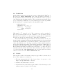
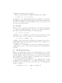
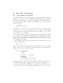
Let’s now put this piece of code into a complete algorithm. The algorithm begins
--algorithm EuclidAlg
where we’ve given it the name EuclidAlg. We next declare the variables
u and v and specify their initial values. (We could omit their initial values
and initialize them with assignment statements, but it’s better to do it this
way.) Just to illustrate the two kinds of initialization, we give u the initial
value 24, but let the initial value of v be any integer from 1 through some
parameter N.
variables u = 24; v ∈ 1.. N;
\∗ ∈ is typed \in .
The declaration of v asserts that its initial value is an element of the set
1 .. N of integers from 1 through N.
We add print statements to print out the initial values of the variables
and the final value of v. The print statement can print the value of any arbitrary expression; to print multiple values, we can either let that expression
be a tuple or else use multiple print statements. The complete algorithm
is as follows, where the while loop is the same as above.
--algorithm EuclidAlg
variables u = 24 ; v ∈ 1 .. N ;
begin a: print hu, vi ;
\∗ h . . . i is typed << . . . >> .
lp: while u 6= 0 do
..
.
end while ;
print h"have gcd", vi ;
end algorithm
5
2.2
The TLA+ Module
The translated version of the algorithm is put inside a TLA+ module. The
algorithm must go in the same file as the module. The module begins
module Euclid
which is typed as
----------------- MODULE Euclid ---------------(The number of dashes in each “-- · · · --” doesn’t matter, as long as there
are at least four.) The module name is arbitrary, but a module named
Euclid must go in a file named Euclid.tla.
The module next imports two standard TLA+ modules.
extends Naturals, TLC
The Naturals module defines common operators on natural numbers, including subtraction (“−”) and the operator “..” that appear in the algorithm’s
expressions. The TLC module is needed if the algorithm uses a print statement. The extends statement must be the first statement in the module.
Next, the module declares the parameter N.
constant N
Every symbol or identifier that appears in an expression in the algorithm
must be either (a) a built-in TLA+ operator like = or h . . . i , (b) declared
or defined in the module, or (c) declared or defined in an imported module.
The module must also contain two single-line comments:
\*
\*
BEGIN TRANSLATION
END TRANSLATION
The translator will delete everything between those two lines and replace it
with the TLA+ translation of the algorithm. The module ends with
which is typed as a string of four or more “ = ” characters.
The algorithm itself may appear in the module within a single comment:
(*
--algorithm EuclidAlg
..
.
end algorithm
*)
It may also be placed before or after the module in file Euclid.tla. However, it is best to put it before the “BEGIN TRANSLATION” line; otherwise,
the line numbers reported in error messages may be wrong.
6
2.3
Translating and Executing the Algorithm
The translator is a Java program. We run it to translate the algorithm by
typing
java pcal.trans Euclid
to a Windows or Unix/Linux command-line window. After translating the
algorithm, we can execute it by running the TLC model checker. The translator creates a configuration file named Euclid.cfg. We must add to that
file a statement that assigns values to the parameters. We assign the value
3000 to the parameter N by putting the statement
CONSTANT N = 3000
in the configuration file. A comment in the file indicates where this statement should go. (The configuration file may contain comments begun by \*
and ended by the end of the line.) We can now run TLC with the command
java tlc.TLC -simulate -depth 200 Euclid
This runs TLC in simulation mode, in which it repeatedly chooses an arbitrary initial value of v in the set 1.. 3000 and executes the algorithm for at
most 200 steps. (If the -depth option is omitted from the command line,
the default value of 100 steps is used.) TLC produces a few lines of output
in which its says what it’s doing when processing the input file, followed by
a gush of output like
<<
<<
<<
<<
<<
<<
<<
<<
<<
24, 1005 >>
"have gcd",
24, 200 >>
"have gcd",
24, 2717 >>
"have gcd",
24, 898 >>
"have gcd",
24, 1809 >>
..
.
3 >>
8 >>
1 >>
2 >>
that ends only when we stop the TLC program (usually by typing a controlC character).
7
Instead of having TLC randomly generate possible executions, we can
run it in model-checking mode, in which it checks all possible executions of
the algorithm. To avoid a huge mass of output, let’s change the configuration
file to have it set N to 4, so there are only 4 possible executions of the
algorithm. We run TLC in model-checking mode by typing
java tlc.TLC Euclid
and it produces the following output:
<<
<<
<<
<<
<<
<<
<<
<<
24, 1
24, 2
24, 3
24, 4
"have
"have
"have
"have
>>
>>
>>
>>
gcd",
gcd",
gcd",
gcd",
4
3
2
1
>>
>>
>>
>>
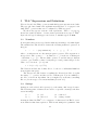
TLC has checked the four possible executions, producing the eight possible
executions of the print statements. But it did not perform those executions separately. Instead, TLC found all reachable states using a breadthfirst search. In doing so, it performed the four possible first steps before
performing any of the four possible last steps.
If you want sensible output from running TLC in model-checking mode,
you should have the algorithm execute only a single print statement at the
end. For our example algorithm, this requires saving the initial value of v
in a separate variable. So, we modify the algorithm by introducing a new
variable v_ini whose initial value is the initial value of v.
--algorithm EuclidAlg
variables u = 24 ; v ∈ 1 .. N ; v_ini = v ;
begin lp: while u 6= 0 do . . .
end while ;
print <<24, v_ini, "have gcd", v>> ;
end algorithm
Translating and running TLC in model-checking mode on this algorithm
produces the output
<<
<<
<<
<<
24,
24,
24,
24,
4,
3,
2,
1,
"have
"have
"have
"have
gcd",
gcd",
gcd",
gcd",
4
3
2
1
>>
>>
>>
>>
8
2.4
Checking the Results
We don’t have to print the results and examine them by hand to check them.
We can let TLC do the checking by using an assert statement. Suppose
we have defined gcd (x , y) to be the gcd of x and y. We can then replace the
print statement in algorithm EuclidAlg by
assert v = gcd(24, v_ini)
TLC will print an error message if this statement is executed when v does not
equal gcd(24, v_ini). For this to work, the operator gcd must be defined
in the TLA+ module, before the translated algorithm—that is, before the
“BEGIN TRANSLATION” line. You may be able to understand the TLA+
definition of gcd knowing that:
• gcd (x , y) is defined to be the largest integer that divides both x and y.
• An integer p divides an integer q iff (if and only if) q % p equals 0,
where q % p is the remainder when q is divided by p.
• The gcd of x and y is at most equal to x (or y).
The standard TLA+ operators that are used in the definition are briefly
explained in Tables 1 and 2 on pages 63 and 64. Here is the definition; give
it a try.
∆
gcd (x , y) = choose i ∈ 1 . . x :
∧x % i =0
∧y % i =0
∧ ∀j ∈ 1 .. x : ∧ x % j = 0
∧y % j =0
⇒i ≥j
If you can’t understand it now, you should be able to after reading Section 5.
2.5
Checking Termination
To check that algorithm EuclidAlg always terminates, we perform the translation with the command
java pcal.trans -translation Euclid
This produces the appropriate translation and configuration file to instruct
TLC to check for termination. If TLC discovers a non-terminating execution, it will print an error message indicating that property Termination is
9
violated and will describe the non-terminating trace. Section 4.4 on page 33
explains how to interpret TLC’s error messages.
You can check an algorithm for termination only if every variable is initialized with a value of the proper type. Here, “variable” means every TLA+
variable declared by the translation. As explained in Section 3.8, these variables include procedure parameters as well as the algorithm’s global variables
and local procedure variables. Procedures are described in Section 3.4, and
page 35 of Section 4.5 explains how to assign initial values to procedure
parameters. If a variable is not initialized, termination checking will cause
TLC to produce a mysterious error message of the form:
Error:
2.6
Attempted to check equality of ...
with ...
{}
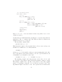
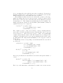
A Multiprocess Algorithm
Algorithm EuclidAlg is a uniprocess algorithm, with only a single thread
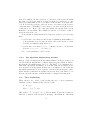
of control. We now look at an example of a multiprocess algorithm written
in +cal. The example is the Fast Mutual Exclusion Algorithm [1]. The
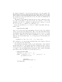
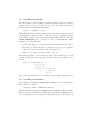
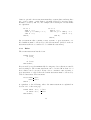
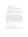
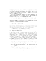
algorithm has N processes, numbered from 1 through N . Figure 1 on the
next page is the original description of process number i , except with the
noncritical section and the outer infinite loop made explicit. Angle brackets
enclose atomic operations (steps). For example, the evaluation of the expression y 6= 0 in the first if statement is performed as a single step. If that
expression equals true, the next step of the process sets b[i ] to false. The
process’s next atomic operation is the execution of the await statement,
which is performed only when y equals 0. (The step cannot be performed
when y is not equal to 0.)
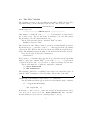
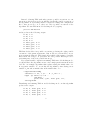
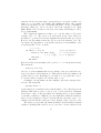
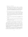
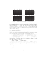
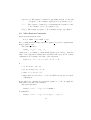
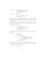
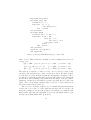
The +cal version of this algorithm is in Figure 2 on page 12. After the
algorithm name comes the declaration of the global variables:
variables x = 0 ; y = 0 ; b = [i ∈ 1.. N 7→ FALSE] ;
The declaration of b states that it is initially an array indexed by the set
1.. N such that b[i] equals FALSE for every i in 1.. N. (The symbol “7→”
is typed “|->”.) The expression
[v ∈ S 7→ v + 1]
equals an array A indexed by the set S such that A[v ] = v + 1 for every v
in S . What programmers call an array, mathematicians call a function. Like
a mathematician, I usually call A a function with domain S rather than an
array indexed by S . However, TLA+ and +cal use programmers’ square
10
ncs: noncritical section;
start: hb[i ] := truei;
hx := i i;
if hy 6= 0i then hb[i ] := falsei;
await hy = 0i;
goto start fi;
hy := i i;
if hx 6= i i then hb[i ] := falsei;
for j := 1 to N do await h¬b[j ]i od;
if hy 6= i i then await hy = 0i;
goto start fi fi;
critical section;
hy := 0i;
hb[i ] := falsei;
goto ncs
Figure 1: Process i of the fast mutual exclusion algorithm, based on the
original description.
brackets instead of mathematicians’ parentheses to represent array/function
application. The 7→ construct and other TLA+ notation for functions is
explained in Section 5.5 on page 45.
The algorithm continues with
process Proc ∈ 1.. N
This statement begins a collection named Proc of N processes, each process
identified by a number in 1.. N. The statement
variable j ;
declares j to be a local variable of these processes, meaning that each of the
N processes has its own separate variable j. A local or global variable z can
be initialized by a declaration of the form
variable z = exp ;
or
variable z ∈ exp ;
The matching “begin” and “end process” enclose the code for each
process in the collection Proc, where self is the identifier of that process (in
this example, a number in 1..N). The correspondence between the original
pseudo-code in Figure 1 and the code for each process self of the +cal
algorithm in Figure 2 should be clear. We represent the noncritical and
11
--algorithm FastMutex
variables x = 0 ; y = 0 ; b = [i ∈ 1..N 7→ FALSE] ;
process Proc ∈ 1..N
variable j ;
begin
ncs: while TRUE do
skip ; \∗ The noncritical section.
start: b[self] := TRUE ;
l1: x := self ;
l2: if y 6= 0 then l3: b[self] := FALSE ;
l4: when y = 0 ;
goto start ;
end if ;
l5: y := self ;
l6: if x 6= self
then l7: b[self] := FALSE ;
j := 1 ;
l8: while j ≤ N do when ~b[j] ;
j := j+1 ;
end while ;
l9: if y 6= self then l10: when y = 0 ;
goto start ;
end if ;
end if;
cs: skip ; \∗ The critical section.
l11: y := 0 ;
l12: b[self] := FALSE ;
end while ;
end process
end algorithm
Figure 2: The fast mutual exclusion algorithm in +cal.
12
critical sections as atomic skip operations whose execution consists of a
single “no-op” step that does nothing. The await statement of the original
version is represented by the +cal when statement. A step containing a
statement “when exp” can be executed only if the expression exp equals
TRUE. Think of the execution of the step as aborting, and having no effect,
if exp equals FALSE.
The original algorithm uses a for loop to test the values of b[j ] in increasing order of j . The for loop is represented in the +cal version by
the while loop at label l8 and the assignment statement that precedes it.
However, the algorithm works if the b[j ] are tested in arbitrary order. We
can rewrite the algorithm to perform the tests in a nondeterministic order
by replacing that +cal code with
j := 1.. N ;
l8: while j 6= {} do
\∗ {} is the empty set.
with p ∈ j do when ~b[p] ;
\∗ ~ is logical negation.
j := j \ {p} ; \∗ \ is set difference.
end with ;
end while
(If you don’t know the meaning of the operator “ \ ”, look it up in the index.)
The statement
with id ∈ S do body
sets id to a nondeterministically chosen element of the set S and then executes body. (In model-checking mode, TLC will check the algorithm for all
possible choices of id .) Replacing id ∈ S with id = exp causes the body to
be executed with id equal to the current value of exp.
A multiprocess algorithm can have multiple “process / end process”
sections. The statement
process Name = e
begins a single process named Name with identifier e. Note that Name is an
arbitrary name that you give to the process; e is an expression. Changing
Name has no effect on the algorithm, but changing the process’s identifier
e can make a difference. Different processes must have different identifiers.
Moreover, the identifiers of all processes should have the same “type”—for
example, they should all be integers or all be strings or all be sets of records.
The safety property that algorithm FastMutex should satisfy is mutual
exclusion, meaning that at most one process can be in its critical section
13
at any one time. For the +cal version, this means that no two processes
can be at the statement labeled cs. An invariant is an assertion that is
true in every state that can occur during an execution of the algorithm.
Mutual exclusion is the invariance of the assertion “no two processes are at
statement cs”. We can tell TLC to check that this assertion is an invariant.
But first, we must know how to express the assertion in TLA+.
The TLA+ translation introduces a new variable pc whose value is the
label of the next statement to be executed. For the uniprocess algorithm
EuclidAlg, the value of pc is the string “lp” iff the next statement to be
executed is the while. The algorithm has terminated iff pc = “Done”.
For a multiprocess algorithm, the variable pc is a function whose domain
is the set of process identifiers. In algorithm FastMutex , a process i is at
statement cs iff pc[i ] equals “cs”. Mutual exclusion is therefore asserted by
the invariance of the predicate Mutex , defined by
∆
Mutex =
∀ i , k ∈ 1 . . N : (i 6= k ) ⇒ ¬((pc[i ] = “cs”) ∧ (pc[k ] = “cs”))
(The operators like ∀, ⇒, ¬, and ∧ are explained in Section 5.3 on page 42.
Section 3.8 on page 27 explains why we could not use the identifier j instead
of k in the ∀ expression.)
TLA+ allows a definition to refer only to variables and operators that
have already been defined or declared. Since the definition of Mutex uses
the variable pc, which is declared by the translation of the algorithm, this
definition must come after the translation—in other words, after the “END
TRANSLATION” line.
We tell TLC to check the invariance of Mutex by adding the following
line to the configuration file.
INVARIANT Mutex
We then run TLC as before, with the command
java tlc.TLC FastMutex
if the algorithm appears in a module also named FastMutex . We tell TLC to
check multiple invariants by listing them in the INVARIANT statement—for
example
INVARIANT Mutex TypeCorrectness Inv3
The variable pc can be used in the algorithm’s expressions We could
therefore also check mutual exclusion by putting the following assert statement in statement cs:
14
∀ i ∈ 1.. N : (i 6= self) ⇒ (pc[i] 6= “cs”)
(“∀” is typed “\A”, and “⇒” is typed “=>”.)
Invariance checking is discussed further in Section 4.5. Section 4.6 describes how to check liveness properties, which are the generalization of
termination.
15
3
The Language
This section lists the statements and constructs of +cal and explains their
meanings. In doing so, it also describes the language’s grammar. A BNF
specification of the grammar appears in Section A on page 54 of the appendix. That grammar and most of the examples in this section show statements
and other syntactic units all ending with a semicolon. That final semicolon
is not required if it is followed by any of the following tokens.
begin do else elsif end macro or procedure process
Before getting to the language description, we need some definitions. A
statement sequence is a sequence of statements, each ended by a semicolon.
For example, the body of a while statement consists of a sequence of statements. If there is an if statement in that sequence of statements, then its
then clause consists of a separate sequence of statements. The statements
in the then clause are not part of the sequence that forms the while’s body.
(It is the if statement, not the statements that occur inside it, that is a
statement of the while’s body.)
A control path is a path through a piece of +cal code that represents a
syntactically possible execution sequence, if we ignore how the statements
are executed. For example, in the code
a: if FALSE then
goto w ;
b: x := 7 ;
c: y := 8 ;
end if ;
d: x := 0 ;
there is a control path that goes from the label a to the label c—even though
no execution can actually follow that path.
A step is a control path that starts at a label, ends at a label, and
passes through no other labels. In the example above, there are two steps
beginning at label a—one that ends at b and one that ends at d. Remember
that there is an implicit label Done at the end of a uniprocess algorithm and
at the end of each process in a multiprocess algorithm. An execution of a
+cal algorithm consists of a sequence of executions of steps. Part of a step
can never be executed by itself (except for a print or assert statement, as
described below).
16
3.1
Expressions
The expressions in +cal algorithms can be any TLA+ expressions that
do not contain a +cal reserved word or symbol such as begin or “||”.
You can write arbitrary TLA+ definitions in the module before the “BEGIN
TRANSLATION” line and use the defined symbols in the algorithm’s expressions. Section 5 explains how to write TLA+ expressions and definitions.
Table 1 on page 63 and Table 2 on page 64 provide a convenient summary.
You are probably used to programming languages that allow only simple
operators in expressions and allow variables to have only simple values. In
+cal, the following statement assigns to x a record whose a component is
the set of integers from 1 to N and whose bcd component is the set of all
prime numbers less than or equal to N.
x := [a
7
→
1..N,
bcd →
7
{i ∈ 2..N : ∀ j ∈ 2..(i-1) : i % j 6= 0} ]
It may be a while before you learn how to take advantage of +cal’s powerful
expression language.
TLA+ has the general rule that an identifier cannot be assigned a new
meaning if it already has a meaning. Thus, the identifier i cannot be used
as a bound variable in an expression like
[i ∈ 1 . . N 7→ false]
if it already has a meaning—for example, if i is an algorithm variable. Assigning a new meaning to a symbol can result in a “multiply-defined symbol”
syntax error in the algorithm’s TLA+ translation.
3.2
The Statements
The examples in Section 2 contain most +cal statements. Here is a complete
list of all the statements that can appear in the body of an algorithm,
process, or procedure, along with the rules for labels that pertain to each of
them. The labeling rules are also all listed in Section 3.7 below.
3.2.1
Assignment
An assignment is either an assignment to a variable such as
y := A + B
or else an assignment to a component, such as
17
x.foo[i+1] := y+3
If the current value of x is a record with a foo component that is a function
(array), then this assignment sets the component x.foo[i+1] to the current
value of y+3. The value of this assignment is undefined if the value of x is not
a record with a foo component, or if x.foo is not a function. Therefore, if
such an assignment appears in the code, then x will usually be initialized to
an element of the correct “type”, or to be a member of some set of elements
of the correct type. For example, the declaration
variable x ∈ [bar : BOOLEAN,
foo : [1.. N → {"on", "off"}] ] ;
asserts that initially x is a record with a bar component that is a Boolean
(equal to TRUE or FALSE) and a foo component that is a function with
domain 1.. N such that x.foo[i] equals either “on” or “off” for each i in
1.. N. (The symbol “→” is typed “->”.)
An assignment statement consists of one or more assignments, separated
by “||” tokens, ending with a semicolon. An assignment statement containing more than one assignment is called a multiple assignment. A multiple
assignment is executed by first evaluating the right-hand sides of all its assignments, and then performing those assignments from left to right. For
example, if i = j = 3, then executing
x[i] := 1 || x[j] := 2
sets x[3] to 2.
Assignments to the same variable cannot be made in two different assignment statements within the same step. In other words, in any control
path, a label must come between two statements that assign to the same
variable. However, assignments to components of the same variable may
appear in a single multiple assignment, as in
x.foo[7] := 13 || y := 27 || x.bar := x.foo ;
3.2.2
If
The if statement has its usual meaning. The statement
if test then t clause else e clause end if ;
is executed by evaluating the expression test and then executing the t clause
or e clause depending on whether test equals true or false. The else
18
clause is optional. An if statement must have a then clause and may have
zero or more elsif . . . then clauses optionally followed by an else clause.
It must be ended by end if;. For example, the following two if statements
are equivalent.
if x > 0
then x := 0;
elsif y > 0 then y := 0;
else z := 0;
end if;
if x > 0
then x := 0
else if y > 0 then y := 0
else z := 0;
end if;
end if;
An if statement that contains a call, return, or goto statement or a
label within it must be followed by a labeled statement. (A label on the if
statement itself is not considered to be within the statement.)
3.2.3
Either
The either statement has the form:
either clause 1
or clause 2
..
.
or clause n
end either ;
It is executed by nondeterministically choosing any clause i that is executable
and executing it. The either statement can be executed iff at least one of
those clauses can be executed. If any clause i contains a call, return, or
goto statement or a label, then the either statement must be followed by
a labeled statement. The statement
if test then t clause
else e clause
end if ;
is equivalent to the following, where the when statement is explained in
Section 3.2.5 on the next page.
either when test ; t clause
or when ¬ test ; e clause
end either ;
19
3.2.4
While
The while statement has its usual meaning. The statement
lb : while test do body end while ;
is executed like the following if statement, where the goto statement is
explained in Section 3.2.11 on page 22.
lb : if test then body ; goto lb ; end if ;
A while statement must be labeled. However, the statement following a
while statement need not be labeled, even if there is a label in its body.
3.2.5
When
A step containing the statement when expr can be executed only when the
value of the Boolean expression expr is TRUE. Although it usually appears
at the beginning of a step, a when statement can appear anywhere within
the step. For example, the following two pieces of code are equivalent.
a : x := y + 1 ;
when x > 0 ;
b : ...
a : when y + 1 > 0 ;
x := y + 1 ;
b : ...
The step from a to b can be executed only when the current value of y+1
is positive. (Remember that an entire step must be executed; part of a step
cannot be executed by itself.)
3.2.6
With
The statement
with id ∈ S do body end with ;
is executed by executing the statement sequence body with identifier id equal
to a nondeterministically chosen element of S . (The symbol ∈ is typed
“\in”.) Execution is impossible if S is empty. This with statement is
therefore equivalent to
when S 6= {} ; with id ∈ S do body end with ;
The two statements
with id = expr do . . .
with id ∈ {expr } do . . .
20
are equivalent. (The expression {expr } equals the set containing a single
element equal to expr .)
In general, a with statement has the form
with id 1 ? expr 1 ; ... ; id n ? expr n do body end with ;
where each ? may be either = or ∈ . This statement is equivalent to
with id 1 ? expr 1 do ... with id n ? expr n
do body end with ... end with ;
The body of a with statement may not contain a label.
3.2.7
Skip
The statement skip; does nothing.
3.2.8
Print
Execution of the statement
print expr ;
is equivalent to skip, except it causes TLC to print the current value of expr .
TLC may print the value even if the step containing the print statement is
not executed because of a when statement that appears later in the step.
An algorithm containing a print statement must be in a module that
extends the TLC module.
3.2.9
Assert
The statement
assert expr ;
is equivalent to skip if expression expr equals true. If expr equals false,
executing the statement causes TLC to produce an error message saying
that the assertion failed and giving the location of the assert statement.
TLC may report a failed assertion even if the step containing the assert
statement is not executed because of a when statement that appears later in
the step.
An algorithm containing an assert statement must be in a module that
extends the TLC module.
21
3.2.10
Call and Return
The call and return statements are described below in Section 3.4 on
page 23.
3.2.11
Goto
Executing the statement
goto lab ;
ends the execution of the current step and causes control to go to the statement labeled lab. In any control path, a goto must be immediately followed
by a label. (Remember that the control path by definition ignores the meaning of the goto and continues to what is syntactically the next statement.)
If is legal for a goto to jump into the middle of a while or if statement,
but this sort of trickery should be avoided.
3.3
Processes
A multiprocess algorithm contains one or more processes. A process begins
in one of two ways:
process ProcName ∈ IdSet
process ProcName = Id
The first form begins a process set, the second an individual process. The
identifier ProcName is the process or process set’s name. The elements of
the set IdSet and the element Id are called process identifiers. The process
identifiers of different processes in the same algorithm must all be different.
This means that the semantics of TLA+ must imply that they are different,
which intuitively usually means that they must be of the same “type”. (For
example, the semantics of TLA+ does not specify whether or not a string
may equal a number.) For execution by TLC, this means that all process
identifiers must be comparable values, as defined on page 264 of the TLA+
book [2].
The name ProcName has no significance; changing it does not change
the meaning of the process statement in any way. The name appears
in the TLA+ translation, and it should be different for different process
statements
As explained above in Section 2.6 on page 10, the process statement is
optionally followed by declarations of local variables. The process body is
22
begun by “begin” and ended by “end process”. Its first statement must be
labeled. Within the body of a process set, self equals the current process’s
identifier.
A multiprocess algorithm is executed by repeatedly choosing an arbitrary
process and executing one step of that process, if that step’s execution is
possible. Execution of the process’s next step is impossible if the process
has terminated, if its next step contains a when statement whose expression
equals false, or if that step contains a statement of the form “when x ∈ S ”
and S equals the empty set. As explained in Section 2.6 on page 10, fairness
conditions may be specified on the choice of which processes’ steps are to
be executed.
3.4
Procedures
An algorithm may have one or more procedures. If it does, the algorithm
must be in a TLA+ module that extends the Sequences module.
The algorithm’s procedures follow its global variable declarations and
define section (if any) and precede the begin of a uniprocess algorithm or
the first process of a multiprocess algorithm. A procedure named PName
begins
procedure PName ( param 1 , . . . , param n )
where the identifiers param i are the formal parameters of the procedure.
These parameters are treated as variables and may be assigned to. As explained in Section 4.5 on page 35, there may also be initial-value assignments
of the parameters. Those initial values are needed by TLC when checking
termination or liveness; they do not affect the algorithm’s execution.
The procedure statement is optionally followed by declarations of variables local to the procedure. These have the same form as the declarations of global variables, except that initializations may only have the form
“variable = expression”. The procedure’s local variables are initialized on
each entry to the procedure.
Any variable declarations are followed by the procedure’s body, which is
begun by “begin” and ended by “end procedure”. The body must begin
with a labeled statement. There is an implicit label Error immediately
after the body. If control ever reaches that point, then execution of either
the process (multiprocess algorithm) or the complete algorithm (uniprocess
algorithm) halts.
A procedure PName can be called by the statement
call PName ( expr 1 , . . . , expr n ) ;
23
Executing this call assigns the current values of the expressions expr i to the
corresponding parameters param i , initializes the procedure’s local variables,
and puts control at the beginning of the procedure body.
A return statement assigns to the parameters and local procedure variables their previous values—that is, the values they had before the procedure
was last called—and returns control to the point immediately following the
call statement.
The call and return statements are considered to be assignments to the
procedure’s parameters and local variables. In particular, they are included
in the rule that a variable can be assigned a value by at most one assignment
statement in a step. For example, if x is a local variable of procedure P ,
then a step within the body of P that (recursively) calls P cannot also assign
a value to x .
For a multiprocess algorithm, the identifier self in the body of a procedure equals the process identifier of the process within which the procedure
is executing.
The return statement has no argument. A +cal procedure does not
explicitly return a value. A value can be returned by having the procedure
set a global variable and having the code immediately following the call
read that variable. For example, in a multiprocess algorithm, procedure P
might use a global variable rVal to return a value by executing
rVal[self] := ... ;
return ;
From within a process in a process set, the code that calls P might look like
this:
call P(17) ;
lab: x := ... rVal[self] ... ;
For a call from within a single process, the code would contain the process’s
identifier instead of self.
In any control path, a return statement must be immediately followed
by a label. A call statement must either be followed in the control path by
a label or else it must appear immediately before a return statement in a
statement sequence.
When a call P statement is followed immediately by a return, the
return from procedure P and the return performed by the return statement
are both executed as part of a single execution step. When these statements
are in the (recursive) procedure P , this combining of the two returns is
essentially the standard optimization of replacing tail recursion by a loop.
24
3.5
Macros
A macro is like a procedure, except that a call of a macro is expanded at
translation time. You can think of a macro as a procedure that is executed
within the step from which it is called.
A macro definition looks much like a procedure declaration—for example:
macro P(s, i) begin when s ≥ i ;
s := s - i ;
end macro ;
The difference is that the body of the macro may contain no labels, no while,
call, return, or goto statement, and no macro call. Macro definitions come
right after any global variable declarations and define section.
A macro call is like a procedure call, except with the call omitted—for
example:
P(sem, y + 17) ;
The translation replaces the macro call with the sequence of statements obtained from the body of the macro definition by substituting the arguments
of the call for the definition’s parameters. Thus, this call of the P macro
expands to:
when sem ≥ (y + 17) ;
sem := sem - (y + 17) ;
When translating a macro call, substitution is syntactic in the sense that
the meaning of any symbol in the macro definition other than a parameter
is the meaning it has in the context of the call. For example, if the body
of the macro definition contains a symbol q and the macro is called within
a “with q ∈ . . .” statement, then the q in the macro expansion is the q
introduced by the with statement.
When replacing a macro by its definition, the translation replaces every
instance of a macro parameter id in an expression within the macro body
by the corresponding expression. Every instance includes any uses of id as
a bound variable, as in the expression
[id ∈ 1 . . N 7→ false]
The substitution of an expression like y + 17 for id here will cause a mysterious error when the translation is parsed. When using +cal, obey the
TLA+ convention of never assigning a new meaning to any identifier that
already has a meaning.
25
3.6
Definitions
An algorithm’s expressions can use any operators defined in the TLA+ module before the “BEGIN TRANSLATION” line. Since the TLA+ declaration of
the algorithm’s variables follows that line, the definitions of those operators
can’t mention any algorithm variables. The +cal define statement allows
you to write TLA+ definitions of operators that depend on the algorithm’s
global variables. For example, suppose the algorithm begins:
--algorithm Test
variables x ∈ 1..N ; y ;
∆
define zy
= y*(x+y)
∆
zx(a) = x*(y-a)
end define ;
...
∆
(The symbol “ = ” is typed “ == ”.) The operators zy and zx can then be
used in expressions anywhere in the remainder of the algorithm. Observe
that there is no semicolon or other separator between the two definitions.
Section 5.11 on page 52 describes how to write TLA+ definitions.
The variables that may appear within the define statement are the ones
declared in the variable statement that immediately precedes it and that
follows the algorithm name, as well as the variable pc and, if there is a procedure, the variable stack . Local process and procedure variables may not
appear in the define statement. The define statement’s definitions need
not mention the algorithm’s variables. You might prefer to put definitions
in the define statement even when they don’t have to go there. However,
remember that the define statement cannot mention any symbols defined
or declared after the “END TRANSLATION” line; and the symbols it defines
cannot be used before the “BEGIN TRANSLATION” line.
3.7
Labels
Various rules for where labels must or may not appear have been introduced
above. The complete set of rules are:
• The first statement in the body of a procedure, of a process, or of a
uniprocess algorithm must be labeled.
• A while statement must be labeled.
• A statement S in a statement sequence must be labeled if it is preceded
in that sequence by any of the following:
26
– A call statement, if S is not a return.
– A return statement.
– A goto statement.
– An if or either statement that contains a labeled statement, a
goto, a call, or a return anywhere within it.
• A macro body and the do clause of a with statement cannot contain
any labeled statements.
• In any control path, a label must come between an assignment to a
variable x and any other statement that assigns a value to x , including
a call or return that sets x if x is a procedure parameter or local
procedure variable.
The implicit labels Done and Error cannot be used as actual labels.
3.8
The Translation’s Definitions and Declarations
This section lists all the identifiers declared and defined in the TLA+ translation of a +cal algorithm. You may need to know what those identifiers
are when writing invariants and liveness properties to check the algorithm.
Moreover, as explained on page 17 of Section 3.1, TLA+ does not allow the
assignment of a new meaning to an identifier that already has a meaning.
Redefining an identifier declared or defined by the translation, or using it as
a bound variable, will cause a “multiply-defined identifier” error when the
TLA+ module is parsed by the SANY parser, which is invoked by TLC.
The translation of a +cal algorithm declares the following TLA+ variables:
• Each variable declared either globally or locally within a process or a
procedure.
• pc
• stack , if the algorithm contains one or more procedures.
• Each formal parameter of a procedure.
A multiprocess +cal algorithm defines each of the following. For a uniprocess algorithm, the “(self )” argument is omitted.
• For a multiprocess algorithm, the set ProcSet of all process identifiers.
27
• The tuple vars of all variables.
• The initial predicate Init. It contains a conjunct for each variable.
The conjuncts for global variables precede those for local procedure
and process variables. The conjuncts for the variables declared in
a single variable statement appear in the order in which they are
declared. (This order is significant, since the initial value of a variable
can depend on the initial values assigned by previous conjuncts.)
• The next-state action Next and the complete specification Spec.
• For each statement label Lab, an action Lab(self ) if the statement is
in a procedure or in a process set; otherwise, an action Lab. This
action is the TLA+ representation of the atomic operation beginning
at that label. (Actions and atomic operations are discussed in Section 5.10.1 on page 49.) If the definition is of Lab(self ), then this is
the action describing the operation performed by a process self , for
self in ProcSet.
• For each procedure P , an action P (self ). It is the disjunction of all
actions in the procedure executed by a process with identifier self in
ProcSet.
• For each process set named P , an action P (self ). It is the disjunction
of all actions not in a procedure that are executed by a process with
identifier self in the process set.
• For each single process named P , an action P that is the disjunction
of all actions not in a procedure that are executed by the process.
Because TLA+ does not allow an identifier to be declared or defined
multiple times, the translation may rename some of these identifiers to produce a legal TLA+ specification. For example, if the +cal code declares a
variable x and also uses x as a label, or if it declares x as a local variable
in two different procedures, then one of the two x’s must be renamed. If
the translator renames identifiers, then it issues a warning and indicates, in
comments placed right after the “BEGIN TRANSLATION” line, what renamings have been done.
Identifiers defined or declared in the translation may not be given new
meanings in any TLA+ definition that follows the “END TRANSLATION” line.
For example, if the +cal algorithm declares a variable j, then a definition
that follows the translated algorithm cannot contain the expression
28
∀i , j ∈ 1..N : (i 6= j ) ⇒ ¬((pc[i ] = “cs”) ∧ (pc[j ] = “cs”))
that redeclares the identifier j . Such a re-use of an identifier causes a
“multiply-defined identifier” error when the TLA+ module is parsed.
29
4
Checking the Algorithm
Sections 2.3–2.5 above tell you how to use the translator and TLC model
checker to check an algorithm. This section explains more about the translator and TLC. Only the commonly used features of TLC are described.
You’ll have to consult Chapter 14 of the TLA+ book for a more complete
description of what TLC can do. Also, check the document Current Versions of the TLA+ Tools on the TLA+ tools web page for recently-added
features. That page can be found from the main TLA+ web page, a link to
which is at http://lamport.org.
TLC takes as input a TLC module and a configuration file. A module
named M is in file M.tla, and its configuration file is named M.cfg. Running the +cal translator on file M rewrites the file M.cfg, creating it anew
if that file doesn’t already exist. (You can keep the translator from writing
or rewriting the configuration file with the -nocfg option.) Normally, you
will let the translator create the configuration file and then add anything
else needed to check the algorithm. If you put those additions where the file
tells you to, they will be preserved when the translator rewrites the file.
4.1
Running the Translator
Running the translator is simple; Section 2.3 on page 7 explains how to do it.
Section 2.5 on page 9 describes the translator’s -termination option. The
other options you are likely to use are ones that specify fairness properties;
they are described in Section 4.6 on page 35. To find out about all the
available options, run the translator with the -help option by typing
java pcal.trans -help
The one part of using the translator that can be tricky is understanding its
messages. The only warning message whose meaning may not be obvious is
Warning: symbols were renamed.
It means that the translator has renamed one or more symbols used in
the algorithm. Section 3.8 on page 27 explains why this was done. The
renamings are listed in the comments within the translation, right after the
“BEGIN TRANSLATION” line.
There are two kinds of translator error messages that can be mysterious.
The first is one saying that the translator was expecting to find a certain
token and didn’t. For example, the missing semicolon at the end of the first
line of
30
L1:
L2:
a := b + c
f[x] := c
produces the error message
-- Expected ";" but found ":="
line . . . , column . . . .
where the line and column numbers indicate the location of the second “:=”.
We might expect the translator to complain when it finds “b + c” followed by
“L2”, since no legal expression can begin b + c L2. However, the translator
does not try to parse expressions. It leaves that task to the SANY parser,
which is used by TLC. Instead, upon seeing the “:=” in the first statement,
the translator just assumes that everything until the next reserved symbol is
part of the assignment statement’s expression. It discovers that something
is wrong when it finds the expression ended by “:=”.
The lesson to be learned from this example is that the source of an error
can come well before the location where the error is reported. If you can’t
find the cause of an error, try narrowing in on it by running the translator
with sections of the code commented out. (You can do this by bracketing
the code with (* and *), even if it contains comments.)
The second class of error that can be mysterious is one caused by omitting a needed label. There are two error messages indicating such an error:
-- Statement at . . . must have a label
-- Multiple assignment to . . .
Section 3.7 on page 26 gives the rules for where labels are needed. The
second message indicates a violation of the rule that, on any control path,
two separate statements that assign a value to the same variable must be
separated by a label. If you are mystified by this message, it may be because you’ve forgotten that call and return statements assign values to a
procedure’s parameters and local variables.
4.2
Specifying the Constants
Most algorithms are written in terms of constant parameters, declared in the
TLA+ module with a constant statement. Those constants must be given
specific values with a CONSTANT statement in the configuration file. You can
also assign new meanings to defined constants and constant operators for
the purpose of model checking. For example, an algorithm might contain a
statement
31
with i ∈ Nat do . . .
where Nat is defined by the standard Naturals module to be the set of
all natural numbers. TLC cannot check an algorithm that requires it to
enumerate an infinite set like Nat. However, you could use the CONSTANT
statement in the configuration file to tell TLC to substitute a finite set of
numbers for Nat.
A CONSTANT statement in the configuration file consists of the keyword
CONSTANT followed by a sequence of assignments and/or replacements, such
as
CONSTANT
N = 13
Proc = {p1, p2, p3}
gcd <- fastGcd
This statement directs TLC to perform three substitutions:
• The assignment N = 13 tells TLC to substitute the number 13 for N ,
where N is a constant either declared or defined in the module.
• The assignment to Proc tells TLC to substitute for Proc the set consisting of the three model values p1, p2, and p3. A model value m is
a special type of value that TLC assumes is unequal to any value it
encounters other than m itself.
• The replacement gcd <- fastGcd tells TLC to substitute for gcd the
value or operator fastGcd , which must be defined in the module. For
example, gcd might be the operator defined as on page 9, and fastGcd
might be an alternative definition that TLC can compute more efficiently. You could use gcd in the algorithm because its definition is
easy to understand, but speed up the checking by having TLC compute
fastGcd instead.
An assignment in a CONSTANT statement has the form Id = exp, where Id
is an identifier and exp is a simple expression. A simple expression is a
number, a string, a model value, or a finite set {e 1 , . . . , e n } where each e i
is a simple expression. A replacement has the form Id 1 <- Id 2, where Id 1
and Id 2 are identifiers, and Id 2 is defined in the module.
TLA+ allows you to declare a constant parameter to be an operator that
takes one or more arguments. For example, the declaration
constant Foo( )
declares Foo to be an unspecified operator that takes a single argument. The
configuration file must use a replacement (“<-”) in a CONSTANT statement
to substitute an operator defined in the module for the parameter Foo.
32
4.3
Constraints
TLC tries to generate all reachable states of the algorithm. It does this by
repeatedly finding all states that can be reached with a single step from a
reachable state that it has already found, starting with all possible initial
states. It will run forever if there are an infinite number of reachable states.
Some algorithms have infinitely many reachable states because they have
counters or queues that can grow without bound. You can limit the reachable states that TLC examines by using a constraint, which is an arbitrary
Boolean expression. If TLC finds a reachable state s that does not satisfy
the constraint, then it will not look for states that can be reached from s.
For example, putting in the TLA+ module the definition
∆
Xsmall = x < 17
and putting in the configuration file the statement
CONSTRAINT Xsmall
causes TLC to find only those reachable states that are either initial states
or are reachable by a sequence of states all having x less than 17.
4.4
Understanding TLC’s Output
When TLC is run, the first thing it does is call the SANY program to parse
the TLA+ module. Parsing may reveal a syntactic error in the module.
The error can be either in the part of the module that you wrote or in the
part written by the translator. The translator does not parse expressions,
leaving it to SANY to find most errors in the algorithm’s expressions. You
should be able to figure out the problem because the translation copies your
expressions pretty much the way you typed them, except for the following
changes.
• Some variables are primed.
• Variables local to a process are turned into functions (arrays) that
take an additional argument. For example, in algorithm FastMutex of
Figure 2 on page 12, each occurrence of the local variable j is replaced
by j [self ].
• An assignment to an element of a function or record variable is rewritten as an assignment to the variable using the TLA+ except construct
explained in Section 5.7 on page 46.
33
• Variables may be renamed, as explained in Section 3.8 on page 27.
If the parser complains that an identifier has been multiply defined, it may
mean that you have redefined or used as a bound variable an identifier that is
defined or declared in the algorithm’s translation. This problem is discussed
above in Section 3.8 on page 27.
Occasionally, it may be difficult to figure out the cause of a parsing error.
In that case, try inserting a “==· · ·==” line to prematurely end the module
in different places until you find the definition or statement that is causing
the error. You can run the parser without running TLC by typing
java tlasany.SANY file
If TLC successfully parses the module and finds no problem with the
configuration file, then it begins executing the algorithm. There are two
kinds of errors it can find: (i) an assert statement is executed when its
expression is false or some property that you asked TLC to check is not
satisfied, or (ii) the algorithm is trying to evaluate a meaningless expression
such as foo.bar if foo does not equal a record. In the first case, TLC tells
you which assertion or property is violated. In the second, it usually prints
out the stack of nested expressions it was executing when it found the error;
but in some cases it just prints the unhelpful message “null”.
For any error, TLC prints out the sequence of states reached in the
execution up to the point at which the error occurred. A state consists of
an assignment of values to all the variables. TLC prints most values as
ordinary TLA+ expressions, as described in Section 5. However, functions
are described in terms of the operators @@ and : > that are defined in the
TLC module. The expression
d 1 : > e 1 @@ d 2 : > e 2 @@ . . . @@ d n : > e n
equals the function f with domain {d 1 , . . . , d n } such that f [d i ] = e i for each
i in 1 . . n.
It can sometimes be quite difficult to figure out the cause of an error
from TLC’s error message. In that case, you can debug by inserting print
statements in the algorithm. You can also use the Print operator in the
algorithm’s expressions or in the invariants that TLC is checking. The operator Print is defined in the TLC module so Print(pval , val ) equals val ,
but TLC prints the value of pval when evaluating it.
34
4.5
Invariance Checking
The examples in Section 2 explain how to use TLC to check invariance of
a formula—meaning that the formula is true in all states reached in any
execution of the algorithm. An important example of invariance is type
correctness. In ordinary typed programming languages, type correctness
is a syntactic condition. Because +cal is typeless, type correctness is a
property of the algorithm, asserting that the value of each variable is an
element of the proper set. For example, we say that a variable p has type
prime number iff the value of p is always a prime number—in other words,
iff the following formula is an invariant, where Nat is the set of natural
numbers.
p ∈ {i ∈ Nat : ∀ j ∈ 2..(i-1) : i % j 6= 0}
(If you don’t understand this invariant now, you should after reading Section 5.) TLC can check if this formula is an invariant. Like type checking in
ordinary programs, checking type correctness is a good way to find simple
errors in a +cal algorithm.
For an algorithm to be type correct, the initial values of its variables
must be of the right “type”. If no initial value is specified for a variable, its
default initial value is {} (the empty set). If {} is not a type-correct value for
the variable, then the algorithm will not be type correct unless the variable
is properly initialized. Among the variables whose type you might want to
check are the procedure parameters. An algorithm can assign initial values
to a procedure’s formal parameters as indicated in this example:
procedure
Foo (p1 = 0, p2 = {"a", "b"})
Like a procedure variable’s declaration, the initial-value declaration of a
formal parameter p must be of the form p = expression.
Since a procedure’s formal parameters are set equal to the corresponding
arguments when the procedure is called, their initial values do not affect the
execution. Those initial values serve only to ensure that the corresponding
variables in the TLA+ specification always have values of the correct type.
4.6
Termination and Liveness
We saw in Section 2.5 how to check termination of a uniprocess algorithm.
Termination is a special case of a general class of properties called liveness
properties, which assert that something must eventually happen. We can
use TLC to check more general liveness properties of an algorithm. As with
35
termination, checking liveness requires that each TLA+ variable be initialized to a value of the proper type. See the discussion of type correctness in
Section 4.5 on the preceding page.
An algorithm satisfies a liveness property only under some assumption—
usually a fairness assumption. There are many possible choices of fairness
conditions that we may want to assume. They can be expressed with the
TLA+ weak and strong fairness operators, WF and SF. A common fairness
assumption for multiprocess algorithms is weak fairness of each process’s
execution. This means that, for each process P , if control in P is at an
operation that it is always possible to execute, then P must eventually
execute that operation. Fairness is discussed in Section 5.10.1 on page 49.
The TLA+ temporal operators used to express fairness and liveness are
described in Section 5.10 on page 49. Temporal properties are subtle and
can be hard to understand. Chapter 8 of the TLA+ book discusses these
properties in more detail.
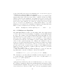
As an example, here is how you can check that algorithm FastMutex of
Section 2.6 satisfies the following property.
Assuming weak fairness of each process’s execution, infinitely often
there is a process in its critical section.
(The algorithm is deadlock and livelock free but not starvation free; it is
possible for all but one process never to enter its critical section.) We run
the translator with the command
java pcal.trans -wf FastMutex
The -wf option instructs the translator to define the specification Spec so it
asserts weak fairness for each process. In the TLA+ module, we define the
formula
∆
Liveness = 23(∃ i ∈ 1 . . N : pc[i ] = “cs”)
which asserts that some process is infinitely often in its critical section.
(The temporal operators 2 and 3 are explained in Section 4.6 on 35.) We
tell TLC to check this property by putting the following statement in the
configuration file.
PROPERTY Liveness
We then run TLC in model-checking mode.
If the liveness property you want to check is termination, you can just use
the translator’s -termination option. It instructs the translator to put the
36
appropriate PROPERTY statement into the configuration file. If no fairness
option is given, the -termination option assumes weak fairness, as if the
-wf option were specified. Use the -nof option to specify that no fairness
condition is to be assumed.
There are many different fairness assumptions one might want to assert
about an algorithm. The translator provides the following additional options
for asserting fairness assumptions.
-sf Strong fairness of each process’s execution.
-wfNext Weak fairness of the entire algorithm’s next-state action.
(This is a weaker assumption than weak fairness for each process.)
-nof Assumes no fairness assumption. This is the default, unless the
-termination option is chosen.
For uniprocess algorithms, the fairness conditions asserted by the -wf, -sf,
and -wfNext options are all equivalent. Algorithm FastMutex satisfies property Liveness under the assumption of weak fairness of the entire algorithm’s
next-state action.
You may want to use a different liveness assumption than the ones provided by these translator options. For example, in a mutual exclusion algorithm like FastMutex , we don’t really want to assume weak fairness of a
process’s execution. That assumption forbids a process from halting in its
noncritical section, but the mutual exclusion problem allows it to do so. It is
not clear whether a process should be allowed to halt in its critical section,
but let’s suppose that it is. What we then want to prove is that, assuming
weak fairness of each process’s execution outside its noncritical and critical
section, if infinitely often there is a process trying to enter its critical section, then infinitely often there is a process in its critical section. From the
list in Section 3.8 of actions defined by the translation, or by examining the
actual translation described in Section B.1 of the appendix, and from the
meaning of the WF operator described in Section 5.10, we find that this
fairness assumption is expressed by the formula
Fairness
∆
= ∀ i ∈ 1 . . N : ∧ WFvars (start(i ))
∧ WFvars (l 1(i ))
∧ WFvars (l 2(i ))
...
∧ WFvars (l 12(i ))
The specification with fairness is therefore
∆
FairSpec = Spec ∧ Fairness
37
To get TLC to use this as the specification, we put the following statement
in the configuration file.
SPECIFICATION FairSpec
If you run the translator after adding this statement, the translator will
remove any SPECIFICATION statement it may have added. Otherwise, you
will have to remove it yourself.
Since a process i is trying to enter its critical section iff pc[i ] 6= “ncs”,
the liveness property we want to check is
CondLiveness
∆
= (23∃ i ∈ 1 . . N : pc[i ] 6= “ncs”) ⇒ Liveness
where Liveness was defined above. We get TLC to check this property by
putting the following statement in the configuration file.
PROPERTY CondLiveness
Remember that when checking any liveness property, the algorithm must
initialize all variables with values of the proper type. Liveness checking
(including termination) is slower than invariance checking, and TLC cannot
check liveness on as large a model as it can check invariance.
4.7
4.7.1
Additional TLC Features
Deadlock Checking
An algorithm is deadlocked if it has not terminated, but it can take no
further step. A process has terminated if it has reached the end of its code,
so control is at the implicit Done label that ends its body.
The most likely way for a uniprocess algorithm to deadlock is for a
procedure call to “fall off the end” without executing a return statement—
that is, for it to reach the implicit label Error that ends the procedure
body.
A multiprocess algorithm is deadlocked if no process can take a step, but
some process has not terminated. The usual way for this to happen is for
each processes to be waiting either at a when statement whose expression
is false or at a statement of the form “with x ∈ S . . . ” when S equals the
empty set.
Deadlock is normally an error and is reported by TLC. However, sometimes an algorithm is supposed to halt in a state in which not all processes
have reached the end of their code. To stop TLC from checking for deadlock,
run it with the -deadlock option.
38
4.7.2
Multithreading
TLC can execute with multiple threads to take advantage of a multiprocessor computer. Running it with the option -workers w tells it to use w
threads. The number w should be at most equal to the number of actual
processors the computer has. (Running it with more threads than there are
processors can slow TLC down.) In theory, using w processors can speed
up TLC’s computation of the set of reachable states by a factor of almost
w . In practice, the speedup depends on the quality of the Java runtime’s
implementation of multithreading. TLC’s algorithm for checking liveness is
single-threaded, so additional worker threads will not speed up that part of
TLC’s execution.
4.7.3
Symmetry
Many algorithms are symmetric in a set of values. For example, the fast mutual exclusion algorithm described in Section 2.6 on page 10 is symmetric in
the set of process identifiers. This means that, given any possible execution
of the algorithm, permuting the set of identifiers of the processes yields a
possible execution. Exactly what symmetry means is explained in Section
14.3.4 on page 245 of the TLA+ book.
We can get TLC to take advantage of symmetry in a set SSet to speed up
its checking of an algorithm. It does this by ignoring any new state it finds
that is the same as a state it has already found under a permutation of the
elements of SSet. We tell it to assume symmetry in SSet as follows. We first
declare SSet to be a parameter of the algorithm, declared in a constant
statement. In the TLA+ module, we define
∆
Perms = Permutations(SSet)
where Permutations is defined in the TLC module, which must be imported
in an extends statement. In the configuration file’s CONSTANT statement,
we substitute a set of model values for SSet—for example, with
CONSTANT SSet = {p1, p2, p3}
(Model values are explained on page 32.) We also add the following statement to the configuration file.
SYMMETRY Perms
TLC can use symmetry only for a set of model values. For TLC to take
advantage of the symmetry of algorithm FastMutex , that algorithm would
39
have to be rewritten to use an arbitrary set of process identifiers instead of
the set of numbers 1 . . N .
We can also tell TLC to assume symmetry in more than one set of
values. For example, an algorithm might be symmetric in both a set SSet
of processes and a set Val of values. We proceed as before, declaring SSet
and Val to be parameters, having TLC substitute sets of model values for
them, and using the same SYMMETRY statement. However, we define Perm
by
∆
Perms = Permutations(SSet) ∪ Permutations(Val )
When we instruct TLC to assume that an algorithm is symmetric, it
does not check whether the algorithm really is symmetric. That’s our responsibility.
Do not tell TLC both to assume symmetry and to check liveness. The
interaction of a symmetry assumption with TLC’s algorithm for checking
liveness is subtle. It’s hard to determine if liveness checking will produce
correct results when symmetry is assumed.
40
5
TLA+ Expressions and Definitions
We now describe the TLA+ operators with which +cal expressions are built.
They are also listed with brief explanations in Tables 1–3 on pages 63–64.
Only TLA+ operators that can be evaluated by TLC are given.
We show the typeset versions of all expressions. Table 5 on page 65
shows how symbols with no obvious ascii representation are typed. TLA+
keywords are typed with upper-case letters, so true is typed as TRUE.
5.1
Numbers
Non-negative integers are typed in the usual way as strings of decimal digits.
The standard module Naturals defines the following standard operators on
integers:
+
−
∗
^ (exponentiation)
<
>
≤
≥
%
÷
..
where − is subtraction, not the unary negation operator. The expression a b
is typed a^b . The operator “ . . ” is defined so a . . b is the set of all integers
c such that a ≤ c ≤ b. The modulus operator % and the integer division
operator ÷ are defined so that, for any integer a and positive integer b, the
value of a % b is in 0 . . (b − 1) and
a = b ∗ (a ÷ b) + (a % b)
The Naturals module also defines Nat to be the set of all natural numbers
(non-negative integers).
The Integers module defines everything the Naturals module does plus
the unary “−” operator and the set Int of all integers. You are unlikely to
use Nat or Int in an algorithm, but you might very well write something
like n ∈ Int in a type-correctness invariant (Section 4.5).
5.2
Strings
Strings are enclosed in double-quotes ("), so the string “abc” is typed "abc".
The following pairs of characters are used to represent certain special characters in strings.
\"
\\
"
\
\t
\n
tab
line feed
\f
\r
form feed
carriage return
A string is defined in TLA+ to be a sequence of characters, but TLC does not
treat them as first-class sequences. TLC treats strings as a primitive data
41
F
true
true
false
false
G
true
false
true
false
F ∧G
true
false
false
false
F
true
true
false
false
G
true
false
true
false
F ∨G
true
true
true
false
F
true
true
false
false
G
true
false
true
false
F ⇒G
true
false
true
true
F
true
true
false
false
G
true
false
true
false
F ≡G
true
false
false
true
Figure 3: Truth tables for the binary Boolean operators.
type, except that the operators “◦” (concatenation) and Len (length) defined
in the standard Sequences module work properly on them—for example,
TLC knows that “ab” ◦ “c” equals “abc” and Len(“abc”) equals 3. (These
operators are described in Section 5.8 on page 47 below.) Even though
sequences in TLA+ are functions, TLC does not regard them as such and it
cannot evaluate “abc”[2].
5.3
Boolean Operators
The Boolean values are written true and false. The set boolean contains
these two values. The five propositional operators on Booleans are
∧ conjunction (and, typed “/\”)
∨ disjunction (or, typed “\/)”
¬ negation (not, typed “ ~ ”)
⇒ implication (typed “ => ”)
≡ equivalence (typed “ <=> ”
or “\equiv”)
The four binary operators are defined by the truth tables of Figure 3 on this
page. The operator ¬ is defined by
¬true = false
¬false = true
In addition to the usual binary operators ∧ and ∨, TLA+ also allows a
bulleted-list notation for conjunctions and disjunctions. For example, the
expression
∧A
∧∨B
∨C
∧D
42
equals A ∧ (B ∨ C ) ∧ D. Indentation is used to eliminate parentheses, which
can make a complicated formula easier to read. The ∧ or ∨ symbols in a
bulleted-list conjunction or disjunction must line up exactly.
Universal and existential quantification over sets of values have the following forms:
∀ x ∈ S : P (x )
The expression that equals true if P (x ) equals true for all elements
x in the set S , and equals false if P (x ) equals false for some x in
S . Thus, ∀ n ∈ 1 . . 3 : f [n] > y is equivalent to
(f [1] > y) ∧ (f [2] > y) ∧ (f [3] > y)
∃ x ∈ S : P (x )
The expression that equals true if P (x ) equals true for some x
in S , and equals false if P (x ) equals false for all x in S . Thus,
∃ n ∈ 1 . . 3 : f [n] > y is equivalent to
(f [1] > y) ∨ (f [2] > y) ∨ (f [3] > y)
In these expressions, the bound identifier x may not already be defined or
declared, and it may not occur in the expression S . In the case of S equal
to the empty set {}, these definitions become
∀ x ∈ {} : P (x ) ≡ true
∃ x ∈ {} : P (x ) ≡ false
for any P . TLA+ allows some obvious abbreviations for nested quantifiers.
For example,
∀ x ∈ S , y ∈ T : F means ∀ x ∈ S : (∀y ∈ T : F )
∃ x, y ∈ S : F
5.4
means ∃ x ∈ S : (∃ y ∈ S : F )
Sets
Enumerated finite sets are written in the usual way, {e 1 , . . . , e n } being the
set containing the elements e 1 , . . . , e n . For example, {1 + 1, 2 + 2, 4} is
the set containing the two elements 2 and 4. (Remember that an element
either is or is not an element of a set; it makes no sense to talk about a set
containing multiple copies of an element.) As a special case of this notation,
43
{} is the empty set (the set containing no elements). TLA+ provides the
following operators on sets.
S
∈ (membership)
∪ (union)
union (big
)
⊆ (subset)
∩ (intersection)
subset (power set)
\ (set difference)
Here are their definitions:
e ∈S
Equals true if e is an element of the set S and equals false
otherwise.
S ∩T
The set of elements in both S and T .
S ∪T
The set of elements in S or T (or both).
S ⊆T
True iff every element of S is an element of T .
S \T
The set of elements in S that are not in T .
union S
The union of the elements of S . In other words, a value e is
an element of union S iff it is an element of an element of S .
S
Mathematicians usually write this as S .
subset S The set of all subsets of S . Mathematicians sometimes call
this the power set of S and write it as P(S ) or 2S .
Mathematicians often describe a set as “the set of all . . . such that . . . ”.
The following two constructs formalize such a description.
{x ∈ S : P (x )} The subset of S consisting of all elements x satisfying
property P (x ). For example, the set of all odd natural
numbers can be written {n ∈ Nat : n % 2 = 1}.
{e(x ) : x ∈ S } The set of elements of the form e(x ), for all x in the
set S . For example, {2∗n + 1 : n ∈ 1 . . 100} is the set
{3, 5, 7, . . . , 201}.
In these expressions, the bound identifier x may not already be defined
or declared, and it may not occur in the expression S . The construct
{e(x ) : x ∈ S } has the same generalizations as ∃x ∈ S : F . For example,
{e(x , y) : x ∈ S , y ∈ T } is the set of all elements of the form e(x , y), for x
in S and y in T .
44
The standard module FiniteSets defines Cardinality(S ) to be the cardinality (number of elements in) the finite set S .
The expression choose x ∈ S : P (x ) is defined to equal some arbitrarily
chosen value x in the set S such that P (x ) equals true. If no such x exists,
then the value of that expression is unspecified, and TLC will report an
error when evaluating it. The choose operator is known to logicians as
Hilbert’s ε. This operator cannot be used to introduce nondeterminism in
an algorithm. The +cal statement
n := CHOOSE i ∈ 1.. 7 :
TRUE
will assign to n the same value every time it is executed. That value is some
single unspecified integer in the set 1 . . 7.
5.5
Functions
What programmers call an array, mathematicians call a function. Intuitively, a function f maps each element d in its domain to the value f [d ].
If f is not a function or d is not in the domain of f , then the meaning of
f [d ] is not specified and TLC will report an error if it tries to evaluate that
expression.
A function is completely specified by its domain and the value of f [d ] for
every d in its domain. If f is a function, then domain f is its domain. The
expression [x ∈ S 7→ e(x )] equals the function f whose domain is S such
that f [d ] = e(d ) for every d in S . For example,
[i ∈ {1, 2, 3} 7→ 2 ∗ i ]
is the function twice with domain {1, 2, 3} such that
twice[1] = 1
twice[2] = 4
twice[3] = 6
Using the operators @@ and : > defined in the TLC module, this function
can also be written
(1 : > 1) @@ (2 : > 4) @@ (3 : > 6)
For any sets S and T , the expression [S → T ] is the set of all functions
f with domain S such that f [d ] is in T for all d in S .
Functions are first-class values, so f [d ] can be a function. For example,
the function
[i ∈ Nat 7→ [j ∈ 1 . . N 7→ (2 ∗ i ) % j ]]
45
is a function f such that f [3][x ] equals 6 % x .
TLA+ also allows functions of multiple arguments. For example,
[i ∈ Nat, j ∈ 1 . . N 7→ (2 ∗ i ) % j ]
is a function g of two arguments such that g[3, x ] equals 6 % x . A function
with multiple arguments is actually a function with a single argument that
is a tuple. For example, g[3, x ] is shorthand for g[h3, x i]. (Section 5.8 on
the next page discusses tuples.)
5.6
Records
TLA+ provides records that are much like the records (also called structs)
of ordinary programming languages. If exp is a record-valued expression,
then exp.bar is the bar field of that record. The expression
[foo 7→ 17, bar 7→ {1, 2, 3}]
equals the record r containing a foo field whose value is 17 and a bar field
whose value is the set {1, 2, 3}. This record r is an element of the set
[foo : Nat, bar : subset 1 . . 13]
consisting of all records with a foo field that is an element of the set Nat of
natural numbers and a bar field that is an element of the set subset 1 . . 13
of all subsets of the set 1 . . 13.
In TLA+, a record with fields foo and bar is actually a function whose
domain is the set {“foo”, “bar”}. The expression exp.bar is shorthand for
exp[“bar”].
5.7
The Except Construct
TLA+ provides an except construct for describing a function or record that
is almost the same as a given function or record. You will probably not need
to use the except construct yourself. However, it is used extensively in the
TLA+ translation of +cal programs, so you must know how to interpret it
if you want to understand the translation.
If f is a function, then [f except ![c] = exp] equals the value of f after
executing the +cal statement f [c] := exp. Thus, [f except ![c] = exp] is
the function g that is the same as f except that g[c] = exp. This function
can also be written
[x ∈ domain f 7→ if x = c then exp else f [x ]]
46
Similarly, if r is a record, then [r except !.c = exp] is the record that
equals the value of r after executing r .c := exp. In other words, it is the
record that is the same as r except that its c field equals exp. Since a record
is a function whose domain is a set of strings, [r except !.c = exp] is the
same as [r except ![“c”] = exp].
A “!” clause of an except construct can be more complicated. For
example [f except ![c].d [e] = exp] is the value of f after executing the
statement f [c].d [e] := exp. You can check that this equals
[f except ![c] = [f [c] except !.d = [f [c].d except ![e] = exp]]]
An except expression can have multiple “!” clauses. For example, the
expression [f except ![c] = exp1, ![d ].e = exp2] equals the value of f after
executing the +cal multiple assignment statement
f [c] : = exp1 | | f [d ].e : = exp2
Remember that a multiple assignment is executed by first evaluating all the
right-hand expressions, then performing the assignments from left to right.
This implies that [f except ![c] = exp1, ![d ].e = exp2] is equal to
[ [f except ![c] = exp1] except ![d ].e = exp2] ].
5.8
Tuples and Sequences
A finite sequence is what programmers usually call a list. In TLA+, a
sequence of length n is the same as an n-tuple, which is defined to be a
function with domain 1 . . n. Finite sequences are written in angle brackets
h i. The sequence he 1 , . . . , e n i is the function s with domain 1 . . n such that
s[i ] equals ei , for each i in 1 . . n. Thus, h“a”, “bc”, “de”i[3] equals “de”.
Sets of tuples can be described with the Cartesian product operator ×.
For example, Nat × Int × {“a”, “b”, “c”} is the set of all triples hx , y, z i such
that x ∈ Nat, y ∈ Int, and z ∈ {“a”, “b”, “c”}.
The standard module Sequences defines the following operators:
Seq(S )
The set of all sequences of elements of the set S . For example,
h3, 7i is an element of Seq(Nat).
Head (s) The first element of sequence s. For example, Head (h3, 7i)
equals 3.
Tail (s) The tail of sequence s, which consists of s with its head removed. For example, Tail (h3, 7, “a”i) equals h7, “a”i.
47
Append (s, e) The sequence obtained by appending element e to the tail
of sequence s. For example, Append (h3, 7i, 3) equals h3, 7, 3i.
s ◦t
The sequence obtained by concatenating the sequences s and
t. For example, h3, 7i ◦ h3i equals h3, 7, 3i.
Len(s)
The length of sequence s. For example, Len(h3, 7i) equals 2.
5.9
Miscellaneous Constructs
An if expression has the form
if bool then t expr else e expr
If bool equals true, then this expression equals t expr ; if bool equals false,
then it equals e expr .
The case expression
case p 1 → e 1 2 . . . 2 p n → e n
equals some e i for which p i equals true. If there is no such p i , then the
value of the expression is unspecified and TLC will report an error when
evaluating it. For example, the value of the expression
case i ∈ 1 . . N → “a” 2 i ∈ N . . 2 ∗ N → “b”
is
• “a” if i is in 1 . . (N − 1),
• “b” if i is in (N + 1) . . 2 ∗ N ,
• either “a” or “b” if i = N ,
• unspecified if i is not in 1 . . 2 ∗ N , and TLC reports an error when
evaluating it.
In the third case, whether the expression equals “a” or “b”, it equals the
same value every time it is evaluated.
The case expression
case p 1 → e 1 2 . . . 2 p n → e n 2 other e
is equivalent to
case p 1 → e 1 2 . . . 2 p n → e n 2 ¬(p 1 ∨ . . . ∨ p n ) → e
48
Thus, its value equals e if all of the p i equal false.
A let expression allows you to make definitions local to the expression.
For example,
∆
let x = a + b
∆
y = a −b
in if y > 0 then x + y else x − y
equals
if a − b > 0 then (a + b) + (a − b) else (a + b) − (a − b)
Any sequence of TLA+ definitions can appear between the let and the in.
Section 5.11 on page 52 describes TLA+ definitions.
5.10
Temporal Operators
A behavior is a nonempty sequence of states, where a state is an assignment of values to variables. A behavior of an algorithm is one that can be
generated by executing the algorithm.
A temporal formula is a predicate on behaviors—in other words, it is
true or false for any nonempty sequence of states. An algorithm satisfies a
temporal formula F iff F is true of all behaviors of the algorithm.
Temporal formulas cannot appear in a +cal algorithm. They are used
only in the fairness properties assumed of the algorithm’s executions and
in the properties asserted about the algorithm. Section 4.6 on page 35
explains how to assert fairness properties of the algorithm and how to tell
TLC to check liveness properties. This section defines the TLA+ temporal
operators that are used to express these fairness and liveness properties.
The definitions are given for infinite behaviors only. They are applied to
finite behaviors by considering the behavior hs 1 , . . . , s n i to be equivalent to
the infinite behavior hs 1 , . . . , s n , s n , s n , . . .i obtained by repeating the last
state forever.
5.10.1
Fairness
An atomic operation of an algorithm consists of all control paths that start
at some label l , end at a label, and do not pass through any label. For
example, this code sequence
49
L1: if x = 0 then y := y + 1
else L2: when sem > 0 ;
sem := sem - 1;
end if;
L3: ...
contains the atomic operations
L1:
if x = 0 then y := y + 1 else L2:
L2:
when sem > 0 ; sem := sem - 1 ; L3:
end if; L3:
and
We name an atomic operation by the label that begins it, so the second of
these atomic operations is called operation L2.
In TLA+, an action is a formula describing how the state changes. More
precisely, it is a formula that is true or false of a pair of states. We say that
s → t is an A step iff action A is true of the pair hs, t i of states. An action
A is said to be enabled in a state s iff it is possible to perform an A action
in state s—that is, iff there is some state t such that s → t is an A step.
For each atomic operation L of a +cal algorithm, the TLA+ translation
defines an action L that represents the operation—in other words, where
s → t is an L step iff executing operation L in state s can produce state
t. We call L an atomic action of the algorithm. Appendix Section B on
page 57 describes how atomic operations are represented as atomic actions.
Fairness assumptions about the algorithm are expressed with the following fairness assumptions about actions:
Weak Fairness of an action A means that if it remains continuously possible to execute A, then A is eventually executed. Weak fairness of A
is expressed by the temporal formula WFvars (A) (typed WF_vars(A)),
where vars is the tuple of all variables of the algorithm. This formula
asserts of a behavior hs 1 , s 2 , . . .i that, if there is some i > 0 such that
A is enabled in state s j , for all j ≥ i , then s j → s j +1 is an A step, for
some j ≥ i .
Strong Fairness of an action A means that if it is repeatedly possible
to execute A, even if it is repeatedly impossible to execute A, then
A is eventually executed. Strong fairness of A is expressed by the
formula SFvars (A) (typed SF_vars(A)). This formula asserts of a behavior hs 1 , s 2 , . . .i that if A is enabled in infinitely many states s j ,
then s j → s j +1 is an A step, for some j > 0.
50
Strong fairness of A is stronger than (implies) weak fairness of A. In other
words, if SFvars (A) is true of a behavior σ, then WFvars (A) is also true of σ.
As an example, let L2 be the atomic action corresponding to the atomic
operation L2 above (on the preceding page). Weak fairness of L2 means
that, if the process is at control point L2 and sem remains positive, then
eventually operation L2 will be executed. Strong fairness of L2 means that,
if the process is at control point L2 and sem keeps being set to a positive
value, even if it keeps being reset to 0, then eventually L2 will be executed.
A process’s next-state action is defined to be the disjunction of all its
atomic actions. The most common fairness assumption is weak fairness of
each process’s next-state action. For a +cal algorithm, weak fairness of a
process’s next-state action is equivalent to the conjunction of weak fairness
of each of its atomic actions. Similarly, strong fairness of a process’s nextstate action in a +cal algorithm is equivalent to strong fairness of each of
its atomic actions. An algorithm’s next-state action is the disjunction of
all of its atomic actions. Weak fairness of the algorithm’s next-state action
means that the algorithm will not halt if it is possible for some process to
perform an action.
5.10.2
Liveness
The temporal properties that an algorithm should satisfy are expressed with
the temporal operators “2”, “3”, and “;”, which are defined as follows:
2F is true of a behavior σ iff the temporal formula F is true for every suffix
of σ. In other words, 2F is true for a behavior hs 1 , s 2 , . . .i iff F is
true on the behavior hs i , s i+1 , . . .i, for all i > 0. Hence, if 2F is true
of σ, then F is true of σ. We usually think of 2F as asserting that F
is always true.
3F is true of a behavior σ iff the temporal formula F is true of some suffix
of σ. Since σ is a suffix of itself, if F is true of σ then so is 3F . We
usually think of 3F as asserting that F is eventually true.
F ; G asserts of a behavior σ that if τ is any suffix of σ for which F is
true, then there is a suffix of τ for which G is true. In other words,
F ; G asserts that whenever F becomes true, G must be true then
or at some later point in the execution. We usually read ; as “leads
to”.
Formulas expressing liveness properties are built with these operators and
state predicates. A state predicate is a formula that is true or false of a
51
state. For example, the state predicate x > 0 is true of those states in which
the value of x is greater than 0. A state predicate is considered to be the
temporal formula that is true of a behavior σ iff it is true of the first state
of σ. If P is a state predicate, then 2P is true of a behavior σ iff P is true
of the first state of all suffixes of the behavior—in other words, iff P is true
of all states of σ. Hence, the temporal formula 2P asserts that P is an
invariant of an algorithm. The formula 3P asserts of a behavior σ that P
is true in some state of σ.
To check that you understand these temporal operators, you can verify
that:
• 23F is true of a behavior σ iff F is true for infinitely many suffixes of
σ. In particular, if P is a state predicate, then 23P asserts of σ that
P is true for infinitely many states of σ.
• 32F is true of a behavior hs 1 , s 2 , . . .i iff there is some i > 0 such that
F is true of hs j , s j +1 , . . .i, for all j ≥ i .
• F ; G is equivalent to 2(F ⇒ 3G).
5.10.3
One Algorithm Implementing Another
Instead of just checking that an algorithm satisfies certain properties, you
can check that it implements a complete higher-level specification describing what the algorithm is supposed to do. The TLA+ book explains how to
write such a specification in TLA+. You can also write the specification as a
more abstract +cal algorithm. In that case, you will have to show that the
algorithm implements its more abstract version under an interface refinement. Interface refinement is explained in Section 10.8 of the TLA+ book.
In most cases, the interface refinement will be a simple data refinement.
5.11
TLA+ Definitions
TLA+ allows you to define operators that take zero or more arguments.
Ordinary operator definitions have the two forms
∆
F = expr
∆
F (p 1 , . . . , p n ) = expr
∆
(The symbol “ = ” is typed “ == ”.) The identifier F and the formal parameters p i must not already have a meaning. All identifiers, other than
52
the p i , that appear in the expression expr must already have a meaning.
Hence, recursive definitions cannot be written in this way. TLA+ does allow
recursive function definitions of the form
∆
f [x ∈ S ] = expr
For example, you can define the factorial function by
∆
fact[n ∈ Nat] = if n = 0 then 1 else n ∗ fact[n − 1]
TLA+ also permits definitions of binary (infix) operators. For example, the
following defines ⊕ (typed “(+)”) to mean addition modulo N :
∆
a ⊕ b = (a + b) % N
Table 4 on page 64 lists all user-definable operator symbols. (Table 5 on
page 65 lists the non-obvious ascii versions of those symbols.)
Definitions of operators or functions that are used in the +cal algorithm
must appear in the module before the “BEGIN TRANSLATION” line, or in a
define statement as described in Section 3.6 on page 26. Except for ones in
a define statement, definitions that use the identifiers declared or defined
in the translation must come after the “END TRANSLATION” line. Those
identifiers are listed in Section 3.8 on page 27.
TLA+ does not use a semicolon or any other delimiter to end a definition.
It’s customary to start each definition on a new line, but that isn’t necessary.
Two successive definitions can be separated by any kind of space character
or characters.
References
[1] Leslie Lamport. A fast mutual exclusion algorithm. ACM Transactions
on Computer Systems, 5(1):1–11, February 1987.
[2] Leslie Lamport. Specifying Systems. Addison-Wesley, Boston, 2003. Also
available on the Web via a link at http://lamport.org.
[3] J. T. Schwartz, R. B. Dewar, E. Schonberg, and E. Dubinsky. Programming with sets: An Introduction to SETL. Springer-Verlag, New York,
1986.
[4] Robert Sedgewick. Algorithms. Addison-Wesley, 1988.
53
Appendix
Section A gives the BNF grammar of +cal, and Section B describes the
TLA+ translation of a +cal algorithm.
A
The Grammar
The algorithm must appear in a file with a TLA+ module, either outside the
module or within a single comment. In the latter case, it will almost surely
be enclosed by “(*” and “*)”. Comments within an algorithm are delimited
by “\*” or “(*. . . *)”. The grammar described here is for an algorithm with
every comment removed and replaced by one or more spaces.
Here is a simplified BNF grammar for the algorithm text. It does not
express the restrictions on where labels must or may not occur, which are
explained in Section 3.7 on page 26. It also does not express the restrictions
on what statements may occur in the body of a macro—namely, that a
while, call, return, goto, or macro call may not appear there. The BNF
uses the following notations.
• The square brackets “ [ ” and “ ] ” are BNF grouping symbols (but “ [ ”
and “ ] ” are literals).
• a | b means a or b.
• a 0,1 means 0 or 1 instance of a.
• a ∗ means 0 or more instances of a.
• a + means 1 or more instances of a.
Any “;” prescribed in the grammar may be omitted if it immediately precedes any of the following reserved words.
begin do else elsif end macro or procedure process
The grammar is:
hAlgorithm i ::= --algorithm hname i
hVarDecls i0,1
hDefinitions i0,1
hMacro i∗
hProcedure i∗
[hAlgorithmBody i | hProcess i+ ]
end algorithm
54
hDefinitions i ::= define hDefs i end define [;]0,1
hMacro i ::= macro hName i ( [hVariable i [, hVariable i]∗ ]0,1 )
hAlgorithmBody i
end macro [;]0,1
hProcedure i ::= procedure hName i ( [hPVarDecl i [, hPVarDecl i]∗ ]0,1 )
hPVarDecls i0,1
hAlgorithmBody i
end procedure [;]0,1
hProcess i ::= process hName i [= | \in] hExpr i
hVarDecls i0,1
hAlgorithmBody i
end process [;]0,1
hVarDecls i ::= [variable | variables] hVarDecl i+
hVarDecl i
::= hVariable i [ [= | \in] hExpr i ]0,1 ;
hPVarDecls i ::= [variable | variables] [hPVarDecl i ;]+
hPVarDecl i
::= hVariable i [ = hExpr i ]0,1
hAlgorithmBody i ::= begin hStmt i+
hStmt i ::= [hLabel i :]0,1 hUnlabeledStmt i
hUnlabeledStmt i ::= hAssign i | hIf i | hWhile i | hEither i | hWith i |
hWhen i | hPrint i | hAssert i | hSkip i | hReturn i |
hGoto i | hCall i | hMacroCall i
hAssign i ::= hLHS i := hExpr i [ || hLHS i := hExpr i]∗ ;
hLHS i ::= hVariable i [[ hExpr i [, hExpr i]∗ ] | . hField i]∗
hIf i ::= if hExpr i then hStmt i+
[elsif hExpr i then hStmt i+ ]∗
[else hStmt i+ ]0,1
end if ;
hWhile i ::= while hExpr i do hStmt i+ end while ;
hEither i ::= either hStmt i+ [or hStmt i+ ]+ end either ;
hWith i ::= with [ hVariable i [= | \in] hExpr i ; ]+
do hStmt i+ end with ;
55
hWhen i ::= when hExpr i ;
hPrint i ::= print hExpr i ;
hAssert i ::= assert hExpr i ;
hSkip i ::= skip ;
hReturn i ::= return ;
hGoto i ::= goto hLabel i ;
hCall i ::= call hMacroCall i
hMacroCall i ::= hName i ( [ hExpr i [, hExpr i]∗ ]0,1 ) ;
hVariable i ::= A TLA+ identifier that is not a +cal reserved word and is
not pc, stack , or self .
hField i
::= A TLA+ record-component label.
hName i
hLabel i
::= A TLA+ identifier that is not a +cal reserved word.
::= A TLA+ identifier that is not a +cal reserved word and is
not Done or Error.
::= A TLA+ expression not containing a +cal reserved word or
symbol.
hExpr i
hDefs i
::= A sequence of TLA+ definitions not containing a
served word or symbol.
+cal
re-
TLA+ expressions and definitions are described in Section 5. A TLA+
record-component label is any sequence of letters, digits, and “_” characters
containing at least one non-digit and not equal to “WF_” or “SF_”. A TLA+
identifier is a record-component that is not one of the following.
ASSUME ASSUMPTION AXIOM CASE CHOOSE CONSTANT
CONSTANTS DOMAIN ELSE ENABLED EXCEPT EXTENDS IF IN
INSTANCE LET LOCAL MODULE OTHER UNION SUBSET THEN
THEOREM UNCHANGED VARIABLE VARIABLES WITH
The +cal reserved words are
assert begin call do either else elsif end goto
if macro or print procedure process return skip
then variable variables while with
The +cal reserved symbols are “:= ” and “||”.
56
B
B.1
The TLA+ Translation
The FastMutex Algorithm
The TLA+ translation is described with the example algorithm of FastMutex
in Figure 2 on page 12. I have simplified the translation a bit to make it
easier to read, but I have not altered its meaning. The translation begins
by declaring the algorithm’s variables and defining vars to be the tuple of
all these variables.
variables x , y, b, j , pc
∆
vars = hx , y, b, j , pci
The variable pc is added to describe the control state. If an algorithm
contains one or more procedures, a variable stack is added to hold the calling
stack. In addition, each formal parameter and local variable of a procedure
is be declared to be a variable.
Had the algorithm contained a define statement, the translation would
have contained two variables statements, the first declaring the variables
x , y, b, and pc, and the second declaring the remaining variable j . The
definitions from the define statement would have been put between the
two variables statements.
For a multiprocess program, the translation next defines the set ProcSet
of all process identifiers.
∆
ProcSet = 1 . . N
Next is the definition of the initial predicate Init that specifies the initial
values of all the declared variables. Comments indicate if the variables are
global or local to a process or procedure.
∆
Init =
Global variables
∧x =0
∧y =0
∧ b = [i ∈ 1 . . N 7→ false]
Process Proc
∧ j = [self ∈ 1 . . N 7→ { } ]
∧ pc = [self ∈ ProcSet 7→ “ncs”]
Observe that the process-local variables and the variable pc are made functions with domain equal to the appropriate set of process identifiers.
Next come the action definitions. As explained in Section 5.10.1 on
page 49, a TLA+ action is a formula describing a pair of states—the state
57
before executing the action and the state after executing it. In an action,
unprimed variables refer to their values before executing the action and the
primed variables refer to their values after the execution.
The translation defines an action for each atomic operation of the algorithm. As explained in Section 5.10.1, an atomic operation begins at a label
that is used to name the action. The first such action definition is generated
by statement ncs. The definition is parameterized by the identifier self ,
which represents the current process’s identifier. (The except construct is
explained in Section 5.7 on page 46.)
∆
ncs(self ) = ∧ pc[self ] = “ncs”
∧ pc 0 = [pc except ![self ] = “start”]
∧ unchanged hx , y, b, j i
The conjunct pc[self ] = “ncs” is an enabling condition, meaning that the
action can be executed only when it is true. It asserts that control of process
self is at label ncs. The action sets pc[self ] to “start”; the unchanged
conjunct asserts that the values of all other variables are not changed. The
evaluation of the while test does not appear explicitly in the action because
it equals true. The skip statement similarly does not appear because it
has no effect.
The atomic actions corresponding to the statements labeled start and l 1
are analogous.
∆
start(self ) = ∧ pc[self ] = “start”
∧ b 0 = [b except ![self ] = true]
∧ pc 0 = [pc except ![self ] = “l1”]
∧ unchanged hx , y, j i
∆
l 1(self ) = ∧ pc[self ] = “l1”
∧ x 0 = self
∧ pc 0 = [pc except ![self ] = “l2”]
∧ unchanged hy, b, j i
Action l 2 performs the if statement’s test and the subsequent transfer of
control.
∆
l 2(self ) = ∧ pc[self ] = “l2”
∧ if y 6= 0 then pc 0 = [pc except ![self ] = “l3”]
else pc 0 = [pc except ![self ] = “l5”]
∧ unchanged hx , y, b, j i
The body of the then clause of statement l 2 consists of two atomic actions.
58
∆
l 3(self ) = ∧ pc[self ] = “l3”
∧ b 0 = [b except ![self ] = false]
∧ pc 0 = [pc except ![self ] = “l4”]
∧ unchanged hx , y, j i
∆
l 4(self ) = ∧ pc[self ] = “l4”
∧y =0
∧ pc 0 = [pc except ![self ] = “start”]
∧ unchanged hx , y, b, j i
The expression y = 0 of the when statement is an enabling condition of
action l 4. (Recall that this means the action can be executed only when
y = 0 is true. The conjunct pc[self ] = “l4” is the other enabling condition
of this action.)
Actions l 5 and l 6 introduce nothing new and their definitions are omitted
here. Action l 7 shows that the process’s local variable j has been turned
into an array indexed by self .
∆
l 7(self ) = ∧ pc[self ] = “l7”
∧ b 0 = [b except ![self ] = false]
∧ j 0 = [j except ![self ] = 1]
∧ pc 0 = [pc except ![self ] = “l8”]
∧ unchanged hx , yi
Action l 8 shows how a while statement whose test is not identically true is
translated.
∆
l 8(self ) = ∧ pc[self ] = “l8”
∧ if j [self ] ≤ N
then ∧ ¬b[j [self ]]
∧ j 0 = [j except ![self ] = j [self ] + 1]
∧ pc 0 = [pc except ![self ] = “l8”]
else ∧ pc 0 = [pc except ![self ] = “l9”]
∧ unchanged j
∧ unchanged hx , y, bi
Actions l 9, cs, and l 11 are obtained in a similar manner and are omitted.
Actions l 10 and l 12 show the translation of an explicit goto and the transfer
of control at the end of the while loop.
∆
l 10(self ) = ∧ pc[self ] = “l10”
∧y =0
59
∧ pc 0 = [pc except ![self ] = “start”]
∧ unchanged hx , y, b, j i
∆
l 12(self ) = ∧ pc[self ] = “l12”
∧ b 0 = [b except ![self ] = false]
∧ pc 0 = [pc except ![self ] = “ncs”]
∧ unchanged hx , y, j i
The translation next defines Proc(self ) to be the next-state action of process
self of process set Proc, which is the disjunction of all the atomic actions
of the process. (The name of a process or process set is used only to name
the process’s next-state action.) A step of the process is one that satisfies
formula Proc(self ).
∆
Proc(self ) = ncs(self ) ∨ start(self ) ∨ l 1(self ) ∨ l 2(self ) ∨ l 3(self )
∨ l 4(self ) ∨ l 5(self ) ∨ l 6(self ) ∨ l 7(self ) ∨ l 8(self )
∨ l 9(self ) ∨ l 10(self ) ∨ cs(self ) ∨ l 11(self )
∨ l 12(self )
The action Next is defined to be the next-state action of the entire algorithm.
It is the disjunction of the next-state actions of all the processes. (The
existential quantification is equivalent to the disjunction Proc(1) ∨ . . . ∨
Proc(N ).)
∆
Next = ∨ ∃ self ∈ 1 . . N : Proc(self ))
∨ Disjunct to prevent deadlock on termination
∧ ∀ self ∈ ProcSet : pc[self ] = “Done”
∧ unchanged vars
The last disjunct of Next is added for TLC’s benefit. TLC has no way of
distinguishing deadlock from termination, which is simply a desired form of
deadlock. The translation therefore adds a disjunction to Next that allows a
terminated algorithm to perform a step that does nothing. This transforms
termination into an infinite no-op loop, so it is not reported as deadlock by
TLC.3 Since the FastMutex algorithm cannot terminate, the disjunct serves
no function in this case. However, the translator is not clever enough to
notice that the disjunct is unnecessary.
The translator next defines formula Spec to be the complete TLA specification of the algorithm. The formula will mean nothing to you if you don’t
know TLA, but that doesn’t matter. You don’t need to understand TLA to
3
If you are familiar with TLA, then you will realize that adding this disjunct does not
change the meaning of the specification, just the way TLC checks it.
60
use +cal. If no liveness or termination option is specified, the definition of
Spec is
∆
Spec = Init ∧ 2[Next]vars
With the -wf option specifying weak fairness of each process, the definition
becomes
∆
Spec = Init ∧ 2[Next]vars ∧ ∀ self ∈ 1 . . N : WFvars (Proc(self ))
If the algorithm had procedures, then Proc(self ) would have been defined
to be the disjunction only of the atomic actions in the process body. For
each procedure P , the translation would have defined action P (self ) to be
the disjunction of the atomic actions in the body of the procedure, and it
would have conjoined to Spec the fairness property
∀self ∈ ProcSet : WFvars (P (self ))
Translation with the -sf option is the same as with the -wf option, except
that WF is replaced everywhere by SF.
Finally, the translation defines the temporal formula Termination that
asserts the property that the algorithm eventually terminates.
∆
Termination = 3(∀ self ∈ ProcSet : pc[self ] = “Done”)
This property is false for every execution of algorithm FastMutex .
B.2
Procedures
The FastMutex algorithm does not show how procedure calls and returns
are translated. Their translation models a standard implementation using
a call stack that is represented by the variable stack . For a multiprocess
algorithm, the value of stack is an array of individual stacks, indexed by
process identifier. You probably don’t care exactly how procedure calls
and returns are represented in TLA+; if you do, you can just look at the
translation of an algorithm containing them. However, you may need to
understand how to read the value of stack when debugging your algorithm.
This is explained with the sample algorithm of Figure 4 on the next page.
An execution of the algorithm calls procedure Q. The execution of Q
calls procedure P , and that execution of P calls Q. The execution of Q
following the last call prints the value of stack and returns. The other two
procedure executions then return and the algorithm terminates.
The value of stack is thus printed in an execution of Q inside an execution
of P inside an execution of Q. Executing the algorithm prints the following
61
--algorithm Procedures
procedure P(pA, pB)
variables pv = 0 ;
begin LP1 : pv := 1 ;
call Q("ProcP") ;
LP2 : return ;
end procedure ;
procedure Q(qA)
variables qv1 = 1; qv2 = 2;
begin LQ1: if qA = "Mn"
then qv1 := 9 ;
call P("a", "b")
else print stack ;
end if ;
LQ2: return ;
end procedure ;
begin LM: call Q("Mn") ;
end algorithm
Figure 4: An algorithm illustrating procedure calls.
value of stack . (The notation for writing records is explained in Section 5.6
on page 5.6.)
h [qA 7→ “Mn”, qv 1 7→ 9, qv 2 7→ 2, pc 7→ “LP2”, procedure 7→ “Q”] ,
[pA 7→ {}, pB 7→ {}, pv 7→ 0,
[qA 7→ {},
pc 7→ “LQ2”, procedure 7→ “P”] ,
qv 1 7→ 1, qv 2 7→ 2, pc 7→ “Done”, procedure 7→ “Q”] i
The value is a sequence of three records, one for each procedure being
executed. The innermost procedure execution produced the first of these
records. The procedure field shows that the algorithm is executing a call of
Q, and the pc field shows that this execution will return to the statement
labeled LP 2. The remaining components show the values of the procedure’s
parameter qA and its local variables qv 1 and qv 2 when the procedure was
called. The corresponding variables will be restored to those values upon
the next return from procedure Q.
The second record in the sequence stack contains the same information
for the call of procedure P . Since this was the first call of P in the call
stack, the parameters pA and pB and the local variable pv contained their
initial values. (Because the algorithm does not specify initial values for pA
and pB , the default initial value {} is used.)
62
Logic
∧ ∨ ¬ ⇒ ≡
true false boolean [the set {true, false}]
∀ x ∈ S : p (1)
∃ x ∈ S : p (1)
choose x ∈ S : p [An x in S satisfying p]
Sets
= 6= ∈
∈
/
{e 1 , . . . , e n }
{x ∈ S : p} (2)
{e : x ∈ S } (1)
subset S
union S
∪ ∩ ⊆ \ [set difference]
[Set consisting of elements e i ]
[Set of elements x in S satisfying p]
[Set of elements e such that x in S ]
[Set of subsets of S ]
[Union of all elements of S ]
Functions
f [e]
domain f
[x ∈ S 7→ e] (1)
[S → T ]
[f except ![e 1 ] = e 2 ]
Records
e.h
[h 1 7→ e 1 , . . . , h n 7→ e n ]
[h 1 : S 1 , . . . , h n : S n ]
[r except !.h = e] (3)
(3)
[Function application]
[Domain of function f ]
[Function f such that f [x ] = e for x ∈ S ]
[Set of functions f with f [x ] ∈ T for x ∈ S ]
[Function b
f equal to f except b
f [e 1 ] = e 2 ]
[The h-field of record e]
[The record whose h i field is e i ]
[Set of all records with h i field in S i ]
[Record b
r equal to r except b
r .h = e]
Tuples
e[i ]
[The i th component of tuple e]
he 1 , . . . , e n i
[The n-tuple whose i th component is e i ]
S 1 × . . . × S n [The set of all n-tuples with i th component in S i ]
(1) x ∈ S may be replaced by a comma-separated list of items v ∈ S , where v is either
a comma-separated list or a tuple of identifiers.
(2) x may be an identifier or tuple of identifiers.
(3) ![e 1 ] or !.h may be replaced by a comma separated list of items !a 1 · · · a n , where
each a i is [e i ] or .h i .
Table 1: The operators of TLA+.
63
if p then e 1 else e 2
[e 1 if p true, else e 2 ]
case p 1 → e 1 2 . . . 2 p n → e n
[Some e i such that p i true]
case p 1 → e 1 2 . . . 2 p n → e n 2 other → e [Some e i such that p i true,
or e if all p i are false]
∆
∆
let d 1 = e 1 . . . d n = e n in e
[e in the context of the definitions]
∧ p 1 [the conjunction p 1 ∧ . . . ∧ p n ]
..
.
∨ p 1 [the disjunction p 1 ∨ . . . ∨ p n ]
..
.
∧ pn
∨ pn
Table 2: Miscellaneous constructs.
2F
3F
WFe (A)
SFe (A)
F ;G
[F is always true]
[F is eventually true]
[Weak fairness for action A]
[Strong fairness for action A]
[F leads to G]
Table 3: Temporal operators.
+ (1)
÷ (1)
⊕ (5)
< (1)
≺
¿
<
⊂
`
∼
°
∝
(1)
(2)
(3)
(4)
(5)
(6)
− (1)
% (1)
ª (5)
> (1)
Â
À
=
⊃
a
'
::=
o
∗ (1)
^ (1,4)
⊗
≤ (1)
¹
<:
v (5)
|=
≈
³
]
/ (2)
. . (1)
®
≥ (1)
º
: >(6)
w
⊇
=|
∼
=
.
=
◦ (3)
...
¯
u
t
++
−−
&
&&
|
?
•
$
%%
@@ (6)
??
∗∗
//
^^
##
$$
!!
Defined by the Naturals, Integers, and Reals modules.
Defined by the Reals module.
Defined by the Sequences module.
x ^y is printed as x y .
Defined by the Bags module.
Defined by the TLC module.
Table 4: User-definable operator symbols.
64
∧
¬
∈
h
<
≤
¿
≺
¹
⊆
⊂
<
v
`
|=
→
∩
u
⊕
ª
¯
⊗
®
∃
∃
]v
WFv
/\ or \land
~ or \lnot or \neg
\in
<<
<
\leq or =< or <=
\ll
\prec
\preceq
\subseteq
\subset
\sqsubset
\sqsubseteq
||=
->
\cap or \intersect
\sqcap
(+) or \oplus
(-) or \ominus
(.) or \odot
(\X) or \otimes
(/) or \oslash
\E
\EE
]_v
WF_v
---------------
∨
≡
∈
/
i
>
≥
À
Â
º
⊇
⊃
=
w
a
=|
←
∪
t
]
×
o
∝
“s”
∀
∀
iv
SFv
\/ or \lor
<=> or \equiv
\notin
>>
>
\geq or >=
\gg
\succ
\succeq
\supseteq
\supset
\sqsupset
\sqsupseteq
-|
=|
<\cup or \union
\sqcup
\uplus
\X or \times
\wr
\propto
"s" (1)
\A
\AA
>>_v
SF_v
⇒
∆
=
6
=
2
3
;
+
−.
7
→
÷
·
◦
•
?
°
∼
'
³
≈
∼
=
.
=
xy
x+
x∗
X#
0
=>
==
# or /=
[]
<>
~>
-+->
|->
\div
\cdot
\o or \circ
\bullet
\star
\bigcirc
\sim
\simeq
\asymp
\approx
\cong
\doteq
x^y (2)
x^+ (2)
x^* (2)
x^# (2)
’
-------========
(3)
(3)
(3)
(3)
(1) s is a sequence of characters.
(2) x and y are any expressions.
(3) a sequence of four or more - or = characters.
Table 5: The ascii representations of typeset symbols.
65
Index
" (double quote), 41
^ (exponentiation), 41
|| (+cal separator), 4
7→ (TLA+ constructor), 10, 46
\ (set difference), 44
\∗ (end-of-line comment), 5
− (minus), 41
¬ (negation), 42
→ (TLA+ operator), 45
; (leads to), 51
÷ (integer division), 41
+ (plus), 41
+cal, 2
expression, 17, 41–49
grammar, 54–56
× (Cartesian product), 47
⇒ (implies), 42
≡ (equivalence), 42
∆
= (defined to equal), 26, 52
. . (integer interval), 6, 41
∗ (multiplication), 41
◦ (sequence concatenation), 48
for strings, 42
2 (always), 51
3 (eventually), 51
< (less than), 41
<- (TLC replacement), 32
≤ (less than or equal), 41
⊆ (subset), 44
(∗ . . . ∗) (comment), 5
f [e] (function application), 10, 45
[h 1 7→ e 1 , . . . , h n 7→ e n ] (record constructor), 46
[x ∈ S 7→ e] (function constructor),
10, 45
[h1 : S1 , . . . , hn : Sn ] (set of records),
46
he 1 , . . . , e n i (tuple/sequence), 47
{ } (empty set), 35, 44
{e 1 , . . . , e n } (set), 43
{x ∈ S : P (x )} (set constructor), 44
{e(x ) : x ∈ S } (set constructor), 44
> (greater than), 41
≥ (greater than or equal), 41
∧ (conjunction), 42
∩ (set intersection), 44
∨ (disjunction), 42
∪ (set union), 44
:> (TLA+ operator), 34, 45
! (in except), 46, 47
% (modulus), 9, 41
@@ (TLA+ operator), 34, 45
∀ (universal quantification), 43
∃ (existential quantification), 43
ε, Hilbert’s, 45
∈ (set membership), 44
in with statement, 20
in variable initialization, 5
action, 50, 57
atomic, 50
corresponding to label, 28
defined for procedure, 28
defined for process set, 28
defined for single process, 28
enabled, 50
next-state, 28, 51, 60
algorithm
beginning of, 5
language, 2
multiprocess, 10
placement of, 6
uniprocess, 10
versus program, 2
66
always (2), 51
and (∧), 42
angle brackets (h i), 47
Append (TLA+ operator), 48
array, 45
ascii representation of symbol, 65
assert (+cal statement), 9, 14, 21
assertion, failure of, 21
assignment, 17–18
in CONSTANT statement, 32
multiple, 4, 18
to a component, 17
assumption, fairness, 36
atomic action, 50
atomic operation, 49
translation of, 58
BEGIN TRANSLATION, 6
behavior, 49
binary operator, defining, 53
BNF grammar, 54
body of process, 22
book, TLA+, 1
Boolean
operator, 42
value, 42
brackets, square, 10
in BNF grammar, 54
built-in operator of TLA+, 6
bulleted list, 42
call (+cal statement), 23
as assignment, 24
not allowed in macro body, 25
translation, 61
Cardinality (TLA+ operator), 45
case (TLA+ expression), 48
cfg file, see configuration file
checking
assertion, 9
invariant, 14, 35
multiple invariants, 14
termination, 9
the algorithm, 30
choose (TLA+ operator), 45
comment
in +cal algorithm, 5, 54
in configuration file, 7
nested, 5
comparable values, 22
component, assignment to, 17
computational complexity, 2
configuration file, 7
rewriting, 30
conjunction (∧), 42
conjunctions, bulleted list of, 42
constant (TLA+ statement), 6, 31
constant
operator, 63
parameters, 31
CONSTANT (TLC cfg file statement),
7, 31, 32
constraint, 33
CONSTRAINT (TLC cfg file statement),
33
constructor, set, 44
control path, 16
data refinement, 52
deadlock, 38, 60
-deadlock (TLC option), 38
debugging, 34
declaration, operator, 32
define (+cal statement), 26
translation of, 57
definition, 52
of binary operator, 53
placement of, 14, 26, 53
-depth (TLC option), 7
difference, set (\), 44
67
disjunction (∨), 42
disjunctions, bulleted list of, 42
division, integer (÷), 41
do (clause of while statement), 20
domain (TLA+ operator), 45
domain of a function, 45
Done (implicit label), 5
not usable as label, 27
not parsed by translator, 31
simple, 32
extends (TLA+ statement), 6
either (+cal statement), 19
when label must follow, 19, 27
else (clause of if statement), 18
elsif (clause of if statement), 19
empty set, 35, 44
enabled, 50
enabling condition, 58
end of module, 6
END TRANSLATION, 6
equivalence (≡), 42
error
found by TLC, 34
found by translator, 30
message, 10
multiply-defined symbol, 17, 27,
29
syntactic, 33
Error (implicit label), 23
not usable as label, 27
Euclid’s algorithm, 4
eventually (3), 51
except (TLA+ construct), 46–47
used in translation, 33, 58
exclusion, mutual, 13
execution of multiprocess algorithm,
23
existential quantification, 43
exponentiation, 41
expression
+cal, 17, 41–49
changed by translator, 33
factorial, definition of, 53
failure of assertion, 21
fairness, 36, 50
false, 42
Fast Mutual Exclusion Algorithm, 10
FastMutex (+cal algorithm), 12, 57
field of record, 46
file name, 6, 30
file, cfg, see configuration file
FiniteSets module, 45
formal parameters of a procedure, 23
initializing, 35
formula, temporal, 49
function, 45
domain of, 45
of multiple arguments, 46
recursive definition of, 53
gcd, 4, 9
Goldbach’s conjecture, 3
Gonthier, Georges, 1
goto (+cal statement), 22
not allowed in macro body, 25
grammar of +cal, 54–56
greatest common divisor, 4, 9
Head (TLA+ operator), 47
-help (translator option), 30
Hilbert’s ε, 45
identifier
defined by translation, 27
process, 22
reassigning meaning of, 17, 25,
27, 28
renamed by translation, 28
if (+cal statement), 18
68
when label must follow, 19, 27
if (TLA+ expression), 48
iff (if and only if), 9
implementing a specification, 52
implementing an algorithm, 52
implication (⇒), 42
imported module, 6
indentation used to eliminate parentheses, 43
infix operator, 64
defining, 53
Init (defined by translation), 28, 57
initial predicate, 28, 57
initializing
procedure parameter, 35
procedure variable, 23
variable, 5, 11, 35
for checking termination, 10
Int (set of integers), 41
integer division (÷), 41
Integers module, 41
interface refinement, 52
intersection (∩), 44
invariant, 14
checking, 14, 35
INVARIANT (TLC cfg file statement),
14
must follow
goto statement, 22, 27
return statement, 24, 27
naming an atomic operation, 50
needed at beginning of
algorithm body, 5, 26
procedure body, 23, 26
process body, 23, 26
not permitted in with statement,
21, 27
of while statement, 20, 26
rules for, 26
language, algorithm, 2
language, programming, 2
leads to (;), 51
Len (TLA+ operator), 48
for strings, 42
list, 47
liveness, 35, 51
checking and symmetry, 40
local variable
declaration, 22
of procedure, 23
of process, 11
macro, 25, 54
call, 25
not allowed in macro body, 25
Java, 7
parameter, 25
macro (+cal statement), 25
keywords, 56
Marzullo, Keith, 1
meaning, reassigning in TLA+, 17,
label, 4, 56
25, 27, 28
action corresponding to, 28
membership, set, 44
after
mode,
call statement, 24, 27
model-checking, 8
either statement, 19, 27
simulation, 7
if statement, 19, 27
model
checker, 7
error caused by omitting, 31
may not appear in macro body, model value, 32
model-checking mode, 8
25, 27
69
module
end of, 6
imported, 6
name, 6
Naturals, 6
TLA+, 6
TLC , 6
modulus (%), 41
multiple arguments, function of, 46
multiple assignment, 4, 18, 31
multiply-defined symbol (parsing error), 17, 27, 29
multiprocess algorithm, 10
execution of, 23
multiprocessor computer, running
TLC on, 39
mutual exclusion, 13
null (TLC error message), 34
numbers, 41
natural, 6
name of
file, 6, 30
module, 6
process, 22
process set, 22, 60
Nat (set of natural numbers), 41
natural numbers, 6
Naturals module, 6, 41
negation (¬), 42
nested comments, 5
nested quantifiers, 43
Next (defined by translation), 28, 60
next-state action
of algorithm, 28, 60
of process, 51
-nocfg (TLC option), 30
-nof (translator option), 37
nondeterminism
in either statement, 19
in with statement, 20
not expressed with choose, 45
not (¬), 42
parameter
as variable, 10
assigning value to, 7
constant, 31
declaration of, 6, 31
of macro, 25
of procedure, 23
initializing, 35
parentheses, eliminated by indentation, 43
parser, 33–34
path, control, 16
pc (variable), 14, 27, 57
in define statement, 26
in expressions, 14
value of, 14
Permutations (TLA+ operator), 39
power set, 44
predicate, initial, 28, 57
predicate, state, 51
print (+cal statement), 5, 8, 21
debugging with, 34
objects, 3
operation, atomic, 49
operator
Boolean, 42
constant, 63
declaration, 32
infix, 64
temporal, 64
TLA+, 41–52
user-definable, 64
or (∨), 42
or (clause of either statement), 19
output of TLC, 33
70
Print (TLA+ operator), 34
procedure, 23
action defined for, 28
call, 23
parameter, 23
as variable, 10
initializing, 35
return from, 24
returning a value, 24
translation of, 61–62
procedure (+cal construct), 23
process, 22
action defined for, 28
body of, 22
identifier of, 22
individual, 22
name of, 22
next-state action of, 51
set, 22
action defined for, 28
name of, 22, 60
variable, 11
process (+cal construct), 11, 22
ProcSet (defined by translation), 27,
57
program versus algorithm, 2
programming language, 2
PROPERTY (TLC cfg file statement),
36
quantification, 43
quantifier nesting, 43
reachable states, 8, 33
record, 46
as function, 46
recursion, tail, 24
recursive definition, 53
refinement, data, 52
refinement, interface, 52
renaming by translation, 28
replacement in CONSTANT statement,
32
reserved words, 56
return (+cal statement), 24
as assignment, 24
not allowed in macro body, 25
translation, 61
rules for labels, 26
SANY parser, 33–34
Sedgewick, Robert, 4
self (+cal identifier), 11, 23, 24, 58
semicolon (;)
not used in TLA+ definitions, 26,
53
omitting, 16, 54
Seq (TLA+ operator), 47
sequence, 47–48
of statements, 16
of states printed by TLC, 34
Sequences Module, 47
set, 43–45
constructor, 44
difference (\), 44
membership, 44
of all . . . , 44
power, 44
process, 22
SETL, 2
SF (TLA+ operator), 36
-sf (translator option), 37, 61
simple expression, 32
-simulate (TLC option), 7
simulation mode, 7
skip (+cal statement), 13, 21
Spec (defined by translation), 28, 60
special character in string, 41
SPECIFICATION (TLC cfg file statement), 38
71
specification of the algorithm, 60
square brackets, 10
in BNF grammar, 54
stack (variable), 27, 57, 61
in define statement, 26
value, 61
state, 34
predicate, 51
reachable, 8, 33
sequence printed by TLC, 34
statement sequence, 16
step, 16, 50
of a +cal algorithm, 4
of an algorithm, 2
string, 41–42
treatment by TLC, 41
strong fairness, 36, 50
struct, 46
subset, 44
subset (TLA+ operator), 44
substitution in TLC, 32
symbol
symbol, ascii representation, 65
typing, 4
user-definable, 64
SYMMETRY (TLC cfg file statement),
39
symmetry used by TLC, 39–40
syntactic error, 33
Tail (TLA+ operator), 47
tail recursion, 24
temporal
formula, 49
operator, 49–52, 64
termination, 35, 60
checking, 9
Termination (property defined by
translation), 9, 61
-termination (translator option), 36
then (clause of if statement), 19
threads, running TLC with multiple,
39
TLA+, 2
book, 1
definition, 52
placement of, 14, 17, 53
module, putting algorithm in, 6
operator, 41–52
tools web page, 30
TLC model checker, 7, 30
error found by, 34
error message, 10
on multiprocessor computer, 39
output of, 33
running, 7
treatment of strings, 41
use of symmetry, 39
TLC module, 6, 34, 39
needed for assert statement, 21
needed for print statement, 21
translation, 57–62
identifiers defined by, 27
identifiers renamed by, 28
of atomic operation, 58
of procedure, 61–62
variables declared by, 27
translator, 6
expressions changed by, 33
running the, 7, 30–31
true, 42
tuple, 47
type correctness, 35
types, 3
typing symbols, 4
unary minus, 41
unchanged (TLA+ operator), 58
union (∪), 44
union (TLA+ operator), 44
72
uniprocess algorithm, 10
universal quantification, 43
user-definable symbol, 64
value
Boolean, 42
model, 32
returned by procedure, 24
values, comparable, 22
variable, 56
declared by translation, 10, 27
initializing, 5, 11, 23, 35
for checking termination, 10
local, declaration of, 22
multiple assignments to, 18, 24,
27
of procedure, 23
of process, 11
variable (+cal statement), 11
vars (defined by translation), 28, 57
weak fairness, 36, 50
web page, TLA+ tools, 30
WF (TLA+ operator), 36
-wf (translator option), 36, 61
-wfNext (translator option), 37
when (+cal statement), 13, 20
while (+cal statement), 20
not allowed in macro body, 25
with (+cal statement), 13, 20
-workers (TLC option), 39
73