1
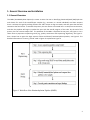
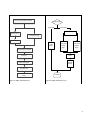
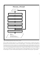
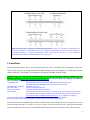
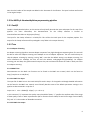
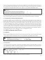
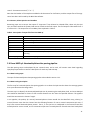
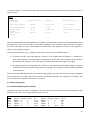
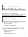
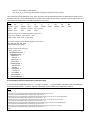
HMPL User Manual Shuying Sun ([email protected] or [email protected]), Texas State University Peng Li ([email protected]), Case Western Reserve University June 18, 2015 Contents 1. General Overview and Installation 2 1.1 General Overview 2 1.2 Installation 5 2. Pipeline Walkthrough 6 2.1 Usage 6 2.2 Initial Input 8 2.3 Pre.HMPL.pl: Hemimethylation preprocessing pipeline 9 2.4 Parse.HMPL.pl: Hemimethylation data parsing pipeline 11 2.5 Testing HMPL using a small dataset and example scripts in the “README” file 16 3. Additional Notes 18 3.1 System Requirements 18 3.2 Running Time 18 4. References 18 1 1. General Overview and Installation 1.1 General Overview The HMPL (HemiMethylation PipeLine) is meant to assist the user in identifying hemimethylated (HM) CpG sites and clusters for each of the two different samples (e.g., cancerous vs. normal individuals) and then compare them. It achieves this goal by utilizing efficient Perl and R scripts to align raw reads, and then parse the data and summarize the final results. To execute this process, the user enters a command line in a Unix/Linux environment, and then the pipeline will begin to update the user with the overall progress of the tasks. By the end of the process, the user receives output files. The workflow of the HMPL is explained in two parts, see Figure 1. Part I shows how to preprocess sequencing reads (e.g., quality assessment and sequencing alignment), see Figure 2. Part II shows how to parse the large amount of data and identify hemimethylation patterns, see Figure 3. The detailed information of “Process_Thread” used in Figure 3 is explained in Figure 4. Figure 1: Workflow of the Hemimethylation Pipeline (HMPL) 2 Assess sequencing qualities using FastQC Get the input options Two input samples One input sample Initialize two Process_Threads Adaptor Trimming Fixed Length Trimming Dynamic Trimming Process_Thread 1: Processing sample 1 Process Sample 1 Process_Thread 2: Processing sample 2 Align sequencing data using BRAT Wait for all threads to finish ACGT-‐count Convert the position from 0-‐based offset to 1-‐based offset Compare the two samples Select the CG sites Combine the forward and reverse strands End of HMPL Figure 2: HMPL workflow Part I. Figure 3: HMPL workflow Part II. 3 Process_Thread Input Data Select CG site greater than the coverage value Identify Hemi-‐methylated CG sites by the high and low cut-‐off values Add annotation for HM sites Identify Singleton (G0) and clusters (G1+G2+G3) Identify reverse clusters (G2+G3) and non-‐reverse clusters (G1) from all clusters(G1 + G2 + G3) Identify consecutive reverse (G2) and non-‐consecutive reverse (G3) from all reverse clusters(G2+G3) by using initial input and all reverse clusters(G2+G3) Output: All HM sites, Singletions (G0), non-‐reverse clusters (G1), consecutive reverse pairs (G2), non-‐consecutive reverse pairs (G3) Figure 4. Detailed explanation of each “Process_Thread”. Note, the HMPL manuscript Figure 1B is an example polarity (or reverse) cluster. The polarity type cluster is generated as the G2 and G3 clusters as shown in the above Figure 4. The G2 polarity cluster only includes two consecutive CpG sites that have a polarity (or reverse) hemimethylation pattern, while G3 polarity cluster consists of two CpG sites that are not consecutive; these two CpG sites are hemimethylated and close to each other, but there is a non-‐hemimethylated CpG site between them. The HMPL manuscript Figure 1 A and C are examples of clusters that are different from Figure 1B, and these clusters are generated together as the G1 cluster as shown in the above Figure 4. In order to make the above explanation clear, the HMPL manuscript Figure 1 is given below. 4 m HMPL manuscript Figure 1: Examples of hemimethylation patterns. M and “C G” represent a “methylated” site. U and “CG” represent an “unmethylated” site. A is an example of hemimethylation occurs on the same strand. B is an example of polarity or reverse hemimethylation pattern with only two CpG sites. C is an example of hemimethylation on different strands with more than two CpG sites. 1.2 Installation Perl (recommend v5.8.8 or later)1, R (recommend v2.13.0 or later)2, and Python 2.6 are required on the user’s system. Then, the user can simply download the HMPL package, and once unzipped, it is ready to go, because FastQC3, BRAT-‐bw4, and cutadapt5 are already pre-‐compiled in the HMPL resources folder. Important note: All script and documentation files can be obtained by downloading the HMPL.zip at the following web link http://hal.case.edu/~sun/HMPL/HMPL.zip. After downloading and unzipping the HMPL.zip, users can obtain the following folders and files: (1) "README" file: Includes detailed information about the HMPL package and example scripts. File name: README.txt & README.pdf, which have the same content. (2) "HMPL.user.manual.pdf": The HPML user manual. (3) "code" folder: Includes all R and Perl code files. (4) "resources" folder: Includes all available software packages. (5) "test.HMPL": A test dataset with 5 million reads, human chromosome 22, reference gene file, and scripts. The test data (5-‐million sequencing reads) can be downloaded from the following web link: http://hal.case.edu/~sun/HMPL/mcf10a.5m.fastq.zip (It is 1.2 GB, after unzipping.) (6) "MCF7.532gene.ge3HM.txt": 532 genes that have ≥ 3 hemimethylated sites in the MCF7 sample More detailed information about these folders and files are given in the above “README” file. We demonstrate the use of HMPL using two publicly available bisulfite-‐treated methylation sequencing datasets for the two 6 cell lines MCF10A and MCF7 in section 2. In this user manual, we mainly show the results of getting hemimethylation patterns for MCF10A, and the results of comparing MCF10A with MCF7 are shown in the Results section of the manuscript. 5 2. Pipeline Walkthrough 2.1 Usage 2.1.1 Using the preprocessing pipeline, part I, Pre.HM.Pipeline.pl The Part I pipeline runs the preprocessing analysis as shown in section 1.1 with the following usage and options (Table 1). perl /<the_diretory_of_HMPL>/code/Pre.HMPL.pl -‐1 <FASTQ_input_file> -‐p <prefix> -‐r <reference_name> [OPTIONS] Table 1. The command options of HMPL Part I (Pre.HMPL.pl) Options [-‐1 <file>] [-‐2 <file>] [-‐o <dir>] [-‐p <string>] [-‐r <file>] [-‐f <sanger or illumina>] [-‐a <yes or no>] [-‐A <stirng>] [-‐T <fix or brat>] [-‐N <int>] [-‐n <int>] [-‐Q <yes or no>] [-‐I <dir>] [-‐i <positive integer>] [-‐m <positive integer>] Explanation Required. FASTQ format single-‐end input file or pair-‐end input file 1, e.g. -‐1 MCF7.fastq, which is the file name of a fastq dataset. FASTQ format pair-‐end input file 2. By default, when there is no input 2, it only processes the input file 1 and processes it as a single-‐end file. The output directory. The default output directory is the user’s current directory. For example, if the current directory in which the user runs HMPL is '/home/user/check.folder/', then when running HMPL command line without specifying '-‐o', the user would have all the output files in '/home/user/check.folder'. Required. The prefix written to the output file names. e.g., –p MCF7, then the output file will have the prefix MCF7 (e.g., MCF7.site, or MCF7.cluster). The name of the file that lists the genome reference sequence (i.e., *.fa) files that users will use to do alignment. Please note that this “-‐r” option must be provided whether or not the “-‐I” (i.e., alignment index) option is provided. Otherwise, the “acgt-‐count” function in the BRAT-‐bw package will not generate proper output files. For example, we set it as “-‐r /home/reference/hg19/hg19.fa.filename.txt” This “hg19.fa.filename.txt” may include the following lines that show the location of the fasta files for chromosomes 10 and 11 (or other chromosomes) as shown below: /home/projects/data/reference/hg19/chr10.fa /home/projects/data/reference/hg19/chr11.fa FASTQ format: HMPL accepts sanger or illumina format FASTQ files as input data; default is sanger. Adapter trimming: Users can select whether or not to utilize cutadapt for adapter trimming (default is no adapter trimming). Adapter sequences: HMPL accepts two adapter sequence inputs, separated by a comma, and default is AGATCGGAAGAGCGGTTCAGCAGGAATGCCGAG,AGATCGGAAGAGCGTCGTGTAGGGAAAGAGTGT. Quality trim flag: Specifies whether to use BRAT dynamic trimming function (default is BRAT-‐trim) or the user can specify ‘fix’ to apply fixed quality trimming (i.e., trim off a fixed number of bases). Fixed quality trimming: Specifies the number of bases to be trimmed at the 5' end (default is 5). Fixed quality trimming: Specifies the number of bases to be trimmed at the 3' end (default is 10). Whether or not to do the quality assessment using FastQC (default is no). The index directory for BRAT-‐bw alignment. If the index folder is provided, it will be automatically used. Otherwise, it will build index, which is the default setting. To specify minimum insert size for paired-‐end mapping, the minimum distance allowed between the leftmost ends of the mapped mates on the forward strand (default is 0). To specify maximum insert size for paired-‐end mapping, the maximum distance allowed between the leftmost ends of the mapped mates on the forward strand (default is 1000). The preprocessing pipeline ties the software and source code together with the appropriate dataflow to ensure correct output is achieved. At this point, users need to have Perl, Python2.6, R, FastQC, and BRAT-‐bw software installed on their system and be able to enter commands in a Unix/Linux environment. 6 The initial FASTQ input files will be discussed in section 2.2. The output directory is the current path, or the path specified by the user, where the output files will be written. 2.1.2 Using the parsing pipeline, part II, Parse.HMPL.pl If the user has finished the hemimethylation preprocessing pipeline and has obtained the files of combined CpG sites, s/he may only run the parsing analysis using our “Parse.HMPL.pl” pipeline with the following usage and options listed in Table 2. perl /<the_diretory_of_HMPL>/code/Parse.HMPL.pl -‐1 <input 1> [OPTIONS] Table 2. The command options of HMPL Part II (Parse.HMPL.pl) Options [-‐1 <file>] Explanation Input file 1 is required. Note: For both Input 1 and Input 2 (see next row), the user can enter two kinds of inputs. One is the combined methylation level data (e.g., “ -‐1 MCF7.CG.combine”), and the other is the “acgt-‐ count” output files, which includes uncombined methylation levels. If it is uncombined, that means the methylation levels on the forward and reverse strands are in two files and they should be separated by comma (,) when providing them as input files, e.g., “-‐1 MCF7.CG.forward,MCF7CG.reverse”. [-‐2 <file>] Input file 2, optional. If specified, the pipeline will process both inputs and compare their final results. Default is only to process the input file 1, and not to do the comparing. Note: For both Input 1 and Input 2, the user can enter two kinds of inputs as explained in the above row. [-‐o <dir>] The output directory where all the output files are created and written. Default is “ <current_dir>/ final.results/ .” [-‐c <int>] The value for selecting the methylation coverage is greater than B. (Default: B=0). On each strand there must be at least B reads to cover a specific CpG site in order for HMPL to check if it is hemimethylated. Changing the “–c” value from a smaller value (e.g., -‐c 5) to a larger value (e.g., -‐c 10) will obtain a shorter list of hemimethylated sites and have a smaller false discovery rate. [-‐l <real>] The cutoff value for selecting low methylation level. (Default: 0.2, range: [0.05, 0.4]). This value corresponds to the “L0” mentioned in Step 4 of the pipeline. If the methylation level is less than this “-‐l” value, it will be claimed as unmethylated. Changing “-‐l” value from a smaller value (e.g., -‐l 0.1) to a larger value (e.g., -‐l 0.2) may give a longer list of hemimethylated sites, but there may be a larger false discovery rate. [-‐h <real>] The cutoff value for selecting high methylation level. (Default: 0.8, range: [0.6, 1]). This value corresponds to the “H0” mentioned in Step 4 of the pipeline. If the methylation level is greater than this “-‐h” value, it will be claimed as methylated. Changing “-‐h” value from a smaller value (e.g., -‐h 0.7) to a larger value (e.g., -‐h 0.9) may give a shorter list of hemimethylated sites, but there may be a smaller false discovery rate. [-‐d <int> ] The maximum distance between two CpG sites to be selected as a cluster with default 50. If the maximum distance is changed from a smaller value (e.g., -‐d 50) to larger value (e.g., -‐d 100), the number of CpG sites in a cluster will be larger, but the total number of hemimethylation clusters will become smaller. [-‐r <file> ] The reference gene file, not the genome reference sequence files. This file is used to provide genetic annotation (i.e., gene names) to the hemimethylation sites. For example, we set it as “-‐r /home/ reference/hg19/refGene.txt”. This “refGene.txt” file contains the gene names and gene information downloaded from the UCSC genome browser. [-‐D <int>] The distance of promoter region (Default: D=1000). That is, if the transcript starting position is located at X=5,000 bp on a chromosome, the promoter region of this gene is defined as from X-‐D = 4,000 to X= 5,000. Note, the "-‐r" options in the Pre.HMPL and Parse.HMPL.pl are different, and this difference is explained below: (1) For the "-‐r" in Pre.HMPL.pl", e.g., "-‐r /home/s_s355/tsu.research/data/reference/hg19/hg19.fa.filename.txt", the contest in hg19.fa.file.name.txt is like: /home/s_s355/tsu.research/data/reference/hg19/chr10.fa /home/s_s355/tsu.research/data/reference/hg19/chr11.fa 7 (2) For the “-‐r” in Parse.HMPL.pl, e.g., “-‐r /home/s_s355/tsu.research/data/reference/hg19/refGene.txt”, it is like 585 NR_026818 chr1 -‐ 34610 36081 36081 36081 3 34610,35276,35720, 35174,35481,36081, 0 FAM138A unk unk -‐1,-‐1,-‐1, 585 NR_026820 chr1 -‐ 34610 36081 36081 36081 3 34610,35276,35720, 35174,35481,36081, 0 FAM138F unk unk -‐1,-‐1,-‐1, 2.2 Initial Input 2.2.1 FASTQ Input File The FASTQ input file contains the raw data that will be analyzed in the upcoming steps. A sample of a FASTQ formatted file is shown below: Box 1 FASTQ input file 1 read: @methy.MCF10A.SRR097806.1 HWW-‐EAS217_0007:6:2:0:815 length=50 NGGTGTTTTTTGGGTTTTAGTAGTTNNGGTTCGTGGTTAGTNNGATTTGT +methy.MCF10A.SRR097806.1 HWW-‐EAS217_0007:6:2:0:815 length=50 !.9768:;;;8547:;;;989526#!!##############!!####### With FASTQ format, there should be 4 lines attributed for every read. The FASTQ input file is the direct input for Steps 1 and 2, and from there, the output files produced will be used as inputs for the remaining steps. 2.2.2 Combined CpG Sites Input File (the initial input for Parse.HMPL.pl, see section 2.1.2) The file with combined CpG sites as input is produced using the “acgt-‐count” function in the BRAT-‐bw software package. The sample file, shown in box 2, has 8 columns without header. The 1st -‐4th columns are the chromosome names, positions, coverage, and methylation for the forward strand. The 5th -‐8th columns are the chromosome names, positions, coverage, and methylation for the reverse strand. Box 2 forward strand chr chr10 chr10 chr10 position coverage methyl 50089 50109 50140 20 0 0 0.1 0 0 reverse strand chr chr10 chr10 chr10 position coverage 50089 50109 50140 10 0 0 methyl 0.9 0 0 chr –chromosome name position – chromosome position of a cytosine site, values in 1-‐based offset. coverage – number of reads methyl – this column displays the methylation data that the bisulfite rate is based on (i.e., bisulfite rate = 1-‐methylation ratio) forward strand – forward chromosome strand (“+”) reverse strand – reverse chromosome strand (“-‐”) 8 Note that the header of the sample was added in this document for clarification. The input has been well-‐sorted in the original output. 2.3 Pre.HMPL.pl: Hemimethylation preprocessing pipeline 2.3.1 FastQC FastQC is already detailed online, so this section will only briefly describe the input and output for this step of the pipeline. For more information, the documentation for the FastQC software is located at www.bioinformatics.bbsrc.ac.uk/projects/fastqc/ The input for the FastQC software is a FASTQ file. This will be the initial input for the complete pipeline. The output for the FastQC software will be packaged in a zip folder in the output directory. 2.3.2 Trim 2.3.2.1 Adapter Trimming An adapter trimming algorithm removes adapter sequences from high-‐throughput sequencing data. The user will be able to utilize the adapter trimming tool cutadapt to trim off adapter sequences. The user could also opt to skip the adapter trimming by entering a string “NO”; note that the default setting is no adapter trimming. For more information on cutadapt, the user can visit the website: code.google.com/p/cutadapt/. For adapter trimming pair-‐end data, the pipeline would compare the pair-‐end data and choose the reads in both pairs after the adapter trimming. 2.3.2.2 BRAT Trim Documentation on the BRAT trim function can be found in the BRAT user manual, which can be found at http://compbio.cs.ucr.edu/brat/. 2.3.2.2.1 BRAT Trim input The input file for BRAT trim is the initial FASTQ file used in Step 1 of the pipeline. Although detailed information can be found in the BRAT user manual, we will briefly describe some of the default parameter settings in the pipeline as demonstrated in script line 3. Script Line 3: trim -‐s $ARGV[0] -‐P $pref -‐q 1 -‐L 64 -‐m 2; In this command, “q” represents the quality score threshold of bases, “L” specifies the smallest value of the range of base quality scores in ASCII representation (64 for illumina format FASTQ file and 33 for sanger format FASTQ file), and “m” is the number of allowable internal N’s. 2.3.2.2.2 BRAT trim output 9 There are a few parameter options that are discussed in the BRAT user manual (and the specific parameters we have implemented are briefly described in the source code notes). However, the output file that is important for the progression of the pipeline will be labeled “prefix_reads1.txt”, and a sample is shown below in box 3. Box 3 prefix_reads1.txt GGGTTTGGTGGTTGGTATTTGTATGTAATTTTAGTTATTTGGGAGGTTG 1 ATCGGAAGAGCGGTTCAGCAGGAATGCCGAGAGCGGAAGAACGGCGTAC ATCGGAAGAGCGGTTCAGCAGGAATGCCGAGATCGGAAGATCGGTTCAT 0 1 1 0 0 In the above sample output, the first column contains the data from the second line of each FASTQ read, followed by the number of bases trimmed at the 5’ end and the 3’ end in the second and third columns, respectively. 2.3.2.3 Fixed Trim (i.e., trimming off fixed number bases) An alternative to BRAT’s dynamic trimming function is a standard fixed-‐trimming option we have included in the pipeline. While utilizing this option, the user has direct control over how many bases to trim from the 5’ end and the 3’ end (Note: These options are listed under global variables in the source code, and the user only has to edit the value corresponding to each variable to set the fixed trim). The input and the output for the fixed trim option are the same as the input and output for BRAT-‐bw alignment, so see section 2.4.1 for more information. Please note that it is good to use this trimming option if users know exactly how many bases they want to trim off and no adapter sequences have been trimmed yet. However, if the users have already trimmed the adapter sequences, then the reads length varies, and it is NOT good to use this trimming option any more. 2.3.3 BRAT-‐bw Alignment and ACGT count 2.3.3.1 BRAT-‐bw BRAT-‐bw handles the alignment of the data. The input is the output from Step 2, and the output will be labeled *.brat, a sample of which is shown below in box 4. For more information, see the BRAT-‐bw user manual. Box 4 trim.single.1M.brat 1 9 13 CGGGGAGTTAGCGTGAGAGGGGGGTTGGGTTAGTTAGTGTTCTTTTTTT chr2 – 3296772 1 3296771 TGGGAAATTATAATGAGATTTGGTTTTCGAGAGTATT chr2 + 74594669 0 74594669 TGGGTTTAAGTAATTTTTTTGTTTTAGTTTTTTAAGTAGTTGAGATC chr2 + 45050947 0 45050947 2.3.3.2 acgt-‐count The input for this part of the pipeline is a bit unusual. Even though it utilizes the output from BRAT-‐bw, the input that is supposed to be included in the execution is actually a one-‐line file containing the name of the output from BRAT-‐bw. The output of “acgt-‐count” is illustrated below in box 5. Box 5 chr start.position end.position CG-‐type:Coverage chr5 chr5 chr5 63004 63004 CHH:0 0 63005 63005 CHH:0 63006 63006 CHH:0 + 0 0 methyl Strand + + CG-‐type – the CG-‐type of a cytosine site, whether it is CpG site or a nonCpG site 10 strand – chromosome strand (“+” or “-‐“) Note that the header of the sample was added in this document for clarification, and the output files of the acgt-‐ count have been well-‐sorted by the BRAT-‐bw software. 2.3.4 Convert, Select CpG sites and Combine Remaining steps are to convert the output of “acgt-‐count” from 0-‐based to 1-‐based offset, select only the CpG sites, and then combine the forward and reverse strands as the final output. The final output is illustrated in box 2 of section 2.2.2. The output files of Pre.HMPL.pl are explained in Table 3: Table 3: Description of output files from Pre.HMPL.pl File name *.CG *_forw.txt *_rev.txt *_reads1.txt *_reads2.txt *_mates1.txt *_mates2.txt Contents The final output of CpG files, the non-‐CpG sites have been already screened out. The file of all acgt sites of forward strand The file of all acgt sites of reverse strand The trimmed FASTQ reads for BRAT-‐bw Another trimmed FASTQ reads for BRAT-‐bw, if the inputs are pair-‐end FASTQ data The file contains reads from the input file whose mates have shorter length after trimming. The file contains reads from the paired input file 2 whose mates have shorter length after trimming. *.brat.mapping.results The BRAT-‐bw Mapping results 2.4 Parse.HMPL.pl: Hemimethylation data parsing pipeline The data parsing steps are developed by our research team, and as such, will contain more detail regarding input/output parameters as well as a description for each step and sub-‐step. 2.4.1 Data Parsing Input The input for hemimethylation data parsing pipeline is described in section 2.2.2. 2.4.2 Data Parsing Description The first step for hemimethylation data parsing pipeline is to select the CpG sites that have the coverage greater than a pre-‐determined coverage value. The next step is to identify the hemimethylated CpG sites by examining the methylation level, and some HM CpG sites would be identified as clusters if their mutual distances are less than the specified distance. The pipeline would also summarize the clusters’ length. In our pipeline, the polarity (or reverse) hemimethylation clusters would also be identified. Here, polarity (or reverse) clusters mean that the clusters have the following features: for two or several consecutive CpG sites, if they have reversed hemimethylation pattern. That is, if one CpG site is methylated in the forward strand and unmethylated in reverse strand, and its consecutive CpG sites is unmethylated in forward strand and methylated 11 in the other strand, or vice versa, then these two CpG sites would be identified as a polarity (or reverse) cluster, as shown in box 6. Box 6 Chromosome: positions Methylation State Coverage Methylation Ratio chr10:346512-346558 MU-UM 20:30;18:33 1:0;0:0.939394 chr10:861689-861694 chr10:12726321272681 chr10:15767541576787 MU-UM MU-UM 5:1;5:1 12:46;13:58 1:0;0:1 1:0;0.0769231:0.896552 MU-UM 2:1;2:1 1:0;0:1 After the identification steps described above, the pipeline would provide annotation for those identified clusters and single sites. There are two kinds of information provided as the annotation: gene information and gene promoter information. The gene names would be annotated for each singleton or clusters if the singleton or cluster is in the range of the gene. For the specified distance L (e.g., L=500 bp), the promoter information is provided as follows: 1. For positive strands, if the single HM site or cluster is in the range/interval of (txtStart – L, txtStart) of a gene, where txtStart is the transcription starting position of this gene, then the gene’s name would be annotated as the promoter. That is, this CpG site is located at the promoter region of this gene. 2. For negative strands, if the single HM site or cluster is in the range/interval of (txtEnd, txtEnd + L) of gene, where txtEnd is the transcription ending position of this gene, then the gene’s name would be annotated as the promoter. If the user has provided two input files to our data parsing pipeline, then after all the previous steps, the pipeline would compare the two inputs and find the common and different HM CpG sites, singletons, and clusters, and then summarize the comparison information in a text file. 2.4.3 Data Parsing Output 2.4.3.1 Hemimethylation CpG sites Output The output files with the suffices “.all.HM.sites” are the text files containing all HM CpG sites identified by high and low cut-‐off values, and a sample output is shown in box 7. Box 7 chr chr10 chr10 chr10 chr10 position 358372 358421 516259 624525 coverage 18 6 7 15 methyl 1 0 0 0 chr chr10 chr10 chr10 chr10 position 358372 358421 516259 624525 coverage 6 7 15 16 methyl 0 1 1 0.875 mu/um MU UM UM UM 12 The output files with suffices “.annotated” are the annotated HM CpG sites, as shown below. The last two columns are the gene and promoter information for CpG sites. Box 8 chr:position chr10:46519904 chr10:49335628 chr10:49335675 chr10:49886908 chr10:50488280 chr10:50503668 patterns M-‐U M-‐U U-‐M M-‐U U-‐M U-‐M coverage 13:90 6:16 6:28 12:6 19:30 14:53 methyl 0.923077:0 1:0 0:0.857143 0.916667:0 0:0.833333 0:0.830189 Gene LOC643650 ARHGAP22 ARHGAP22 NA CHAT CHAT Promoter NA NA NA NA SLC18A3 NA The output files with suffices “.Singleton” (G0) have the similar output format as shown in Box 9, but it is the selected single CpG sites. 2.4.3.2 Hemimethylation Clusters Output The output files with suffices “.Clusters” are the hemimethylation clusters. Box 9 gives an example of this output. It has the similar output format as Box 8 in spite of the additional last two columns that indicate the length of the clusters in bps, and the number of CpG sites within the clusters. Box 9 Chr:positions Pattern coverage chr17:11084428-11084474 MU-UM 21:11;24:13 chr17:15795888-15795934 MU-UM 19:17;17:23 chr17:16547718-16547766 MU-UM 22:12;11:13 chr17:16857943-16857989 MU-UM 33:16;32:16 chr17:17553158-17553206 MU-UM 23:8;22:8 chr17:18516721-18516724-18516727-18516731-18516740 FOXO3B;ZNF286B NA chr17:22781527-22781574 MU-UM 11:11;7:13 chr17:26743508-26743557 MU-UM 39:19;29:26 chr17:26865386-26865435 MU-UM 8:10;7:11 chr17:30327477-30327526 MU-UM 19:6;17:7 chr17:31973165-31973210 MU-UM 11:11;9:12 chr17:33738671-33738718 MU-UM 9:21;8:20 methyl gene 0.952381:0.0909091;0.125:0.846154 1:0;0:0.869565 ADORA2B 1:0;0:1 CCDC144A NA 0.939394:0;0:1 NA 1:0;0:1 RAI1 NA MMMMM-UUUUU 28:6;28:6;23:6;16:6;11:6 20 5 0.818182:0.0909091;0.142857:0.923077 1:0;0:1 RAB11FIP4 NA 0.875:0;0:0.818182 RAB11FIP4 1:0;0:1 NA NA 1:0;0:1 NA NA 1:0;0:1 GPR179 NA NA SHISA6 47 2 NA 47 2 49 2 NA 47 2 49 2 0.928571:0;1:0;0.956522:0;0.9375:0;0.909091:0 LOC440419 50 NA 50 46 48 promoter NA 2 50 2 2 2 length 48 #ofCG 2 2 There are in total four kinds of “.Clusters ” output files as shown below: *.all.HM.Clusters: All the HM clusters. *.all.Rev.Clusters: All reversed clusters *.non.Rev.Clusters (G1): non-‐reversed clusters *.non.consec.revs.Clusters (G2): non-‐consecutive reversed clusters *.consec.revs.Clusters (G3): consecutive reversed clusters. Only the first one has the last two additional columns as shown in Box 10. The output files with suffices “.summary” is the summary of HM sites and clusters for this input. It includes four kinds of information, separated by two new lines, as shown in box 10. The first table summarizes the number of “M”, “U”, and “P” in each strand, and the number of each combination of “M”, “U”, and “P” in both strands. all_CG_gr5: indicates the number of all the CpG sites which has the coverage greater than 5. The “5” was specified by the user. HM: the number of all the hemimethylated CpG sites. MU: the number of all the hemimethylated CpG sites that are methylated in the forward strand and unmethylated in the reverse strand. UM: the number of all the hemimethylated CpG sites which are unmethylated in the forward strand and methylated in the reverse strand. Singleton: hemimethylated CpG sites exist as singletons. 13 Clusters: the number of HM clusters. CpG_sites_as_in_clustering: the number of CpG sites existed in all the clusters. Two summaries of the HM cluster sizes, basic summary, and the quantile summary are generated as shown in the example in box 10. Here, the HM cluster size means the number of CpG sites in a cluster. The last part of box 10 summarizes the frequencies of all HM state patterns of clusters. Box 10 Sample +M +U +P -‐M -‐U MCF10A 73558 159849 53027 73501 159695 Sample HM Singleton Clusters CG_in_clusters MCF10A 6712 3353 1666 3359 The basic summary of the Hemimethylation cluster size is Min. 1st Qu. Median Mean 3rd Qu. Max. 2.000 2.000 2.000 2.016 2.000 6.000 The quantile summary of the Hemimethylation cluster size is 0% 50% 90% 95% 99% 100% 2.00 2.00 2.00 2.00 2.35 6.00 The pattern frequencies summary: cluster_pattern Freq 1 MMMMMM-‐UUUUUU 1 2 MMMMM-‐UUUUU 1 3 MMM-‐UUU 1 4 MM-‐UU 8 5 MMU-‐UUM 2 6 MUM-‐UMU 1 7 MUMU-‐UMUM 2 8 MU-‐UM 1627 9 UM-‐MU 3 10 UMU-‐MUM 3 11 UU-‐MM 11 12 UUU-‐MMM 4 13 UUUU-‐MMMM 1 14 UUUUU-‐MMMMM 1 -‐P 53238 UU 147974 UP 8505 UM 3370 … … 2.4.3.3 Common CpG sites and Clusters in both two inputs If the user has provided two inputs, i.e. “…-‐1 input1 -‐2 input2…”, the Parse.HMPL.pl would provide five additional output files with suffices “.compare”, and the output files of Parse.HMPL.pl are explained in Table 4. Box 11 ##### Summary: common HM lines for /home/pxl119/8.10.2013/MCF10.MCF7.gr5/MCF10A.gr5.non.Rev.Clusters and /home/pxl119/8.10.2013/MCF10.MCF7.gr5/MCF7.gr5.non.Rev.Clusters: 8 HemiMethylated lines in /home/pxl119/8.10.2013/MCF10.MCF7.gr5/MCF10A.gr5.non.Rev.Clusters but not HemiMethylated in /home/pxl119/8.10.2013/MCF10.MCF7.gr5/MCF7.gr5.non.Rev.Clusters: 16 HemiMethylated lines in /home/pxl119/8.10.2013/MCF10.MCF7.gr5/MCF10A.gr5.non.Rev.Clusters but no coverage in /home/pxl119/8.10.2013/MCF10.MCF7.gr5/MCF7.gr5.non.Rev.Clusters: 12 HemiMethylated lines in /home/pxl119/8.10.2013/MCF10.MCF7.gr5/MCF7.gr5.non.Rev.Clusters but not HemiMethylated in /home/pxl119/8.10.2013/MCF10.MCF7.gr5/MCF10A.gr5.non.Rev.Clusters: 21 HemiMethylated lines in /home/pxl119/8.10.2013/MCF10.MCF7.gr5/MCF7.gr5.non.Rev.Clusters but no coverage in /home/pxl119/8.10.2013/MCF10.MCF7.gr5/MCF10A.gr5.non.Rev.Clusters: 53 ##### 14 common HM lines for /home/pxl119/8.10.2013/MCF10.MCF7.gr5/MCF10A.gr5.non.Rev.Clusters and /home/pxl119/8.10.2013/MCF10.MCF7.gr5/MCF7.gr5.non.Rev.Clusters: chr12:131845661-‐131845705-‐131845749-‐131845792 MUMU-‐UMUM 71:30;45:34;21:21;15:24 0.915493:0;0:0.970588;0.952381:0;0:1 ** MUMU-‐UMUM 88:55;55:56;28:27;13:28 0.988636:0.0363636;0.0181818:0.982143;0.964286:0;0:0.928571 ANKLE2 NA chr19:2082837-‐2082839-‐2082848 UUU-‐MMM 32:34;32:34;32:38 0.03125:0.970588;0.03125:1;0.03125:1 ** UUU-‐MMM 22:27;22:29;22:30 0:1;0:0.965517;0:0.966667 AP3D1 NA chr19:38979454-‐38979463 UU-‐MM 20:9;12:9 0:1;0:1 ** UU-‐MM 28:9;20:9 0:1;0:0.888889 NA KCTD15 chr1:9181489-‐9181519-‐9181565 UMU-‐MUM 9:12;18:31;9:34 0:0.916667;1:0.0322581;0:0.911765 ** UMU-‐MUM 16:13;19:31;10:37 0:0.923077;0.947368:0.0322581;0:0.891892 NA NA chr2:53940411-‐53940424-‐53940473 UMU-‐MUM 17:26;27:35;24:40 0:1;1:0.0571429;0.0833333:0.925 ** UMU-‐MUM 16:23;39:56;29:61 0:1;1:0.0357143;0.0689655:0.967213 GPR75;GPR75-‐ASB3 NA chr2:132731365-‐132731375 MM-‐UU 53:123;53:121 0.981132:0.0162602;0.962264:0 ** MM-‐UU 63:155;62:155 0.920635:0;0.951613:0 ANKRD30BL MIR663B chr6:151704347-‐151704394-‐151704424 MUM-‐UMU 30:21;22:31;8:17 0.966667:0;0:0.967742;1:0 ** MUM-‐UMU 25:35;15:47;12:27 0.88:0;0:0.829787;0.916667:0.037037 AKAP12 NA chrY:10644075-‐10644103 MM-‐UU 11:13;11:21 1:0;0.909091:0 ** MM-‐UU 21:11;21:13 0.904762:0;1:0 NA NA Table 4. The description of output files of Parse.HMPL.pl: File names *.grX *.all.HM.sites *.all.HM.sites.annotated *.all.labelled.CG *. Summary *.all.HMClusters *.all.Rev.Clusters *.non.Rev.Clusters (G1) *.Singleton (G0) *.consec.revs.Clusters (G3) *.non.consec.revs.Clusters (G2) *.compare Contents The CpG sites with coverage greater than X. The hemimethylated CpG sites identified by the high and low cut-‐off values. The annotated hemimethylated sites (i.e., gene names are provided). The CpG sites with coverage greater than X and with the labels of methylation states (P: partially methylated, M: methylated, U: unmethylated). The summary file for all the methylation states of single hemimethylation sites and clusters. All hemimethylated clusters. All of the polarity (or reverse) clusters, including both consecutive and non-‐consecutive polarity clusters. The hemimethylated clusters that are not polarity patterns. Single hemimethylated CpG sites. The consecutive polarity (or reverse) clusters (i.e., with just two consecutive CpG sites). The non-‐consecutive polarity clusters (i.e., with two CpG sites that are not consecutive). The results of comparing two samples. 2.5 Testing HMPL using a small dataset and example scripts in the “README” file In order to make it easy for users to test the HMPL, we have prepared a small dataset with 5 million reads (a FASTQ *.fastq file), the human chromosome 22 reference sequence (a FASTA .fa file), and the example scripts to run this small methylation dataset by aligning it to chromosome 22 and identify hemimethylated sites using both Part I and Part II of HMPL. The user simply needs to download the data, install the HMPL package, and then change the data path/directory in the example script accordingly to be able to run the HMPL. It only takes 11 minutes to run this small dataset using a Linux computer with 4 GB RAM. The 5-‐million-‐read small dataset, human chromosome 22, and the example script are included in a folder named “test.HMPL”. Once users 15 download the HMPL.zip file from the web link http://hal.case.edu/~sun/HMPL/HMPL.zip, and unzip it, they will be able to see this “test.HMPL’ folder. This folder includes the following files: 1) “Test.data.txt” explains how to download the small dataset of 5-‐million sequencing reads (file name: mcf10a.5m.fastq). In fact, the test data (5-‐million sequencing reads) can be downloaded from the following web link: http://hal.case.edu/~sun/HMPL/mcf10a.5m.fastq.zip (It is 1.2 GB, after unzipping.) 2) Related genome reference files (file name: chr22.fa and refGene.txt), 3) The scripts of testing how to run HMPL using the small dataset. The test script file name is "small.data.script.txt" and "small.data.script.pdf", these two files have the same content. To make it easier for user, the content of this test script file is provided in the following box. ##################################################################################### # 1. download and unzip the latest HMPL: wget http://hal.case.edu/~sun/HMPL/HMPL.zip unzip HMPL.zip -‐d HMPL_new ##################################################################################### # 2. Create a folder to run HMPL mkdir 2015.6.6.HMPL.QA cd 2015.6.6.HMPL.QA/ pwd # check the present working directory, then get /home/pxl119/2015.6.6.HMPL.QA ##################################################################################### # 3. The following are step by step scripts and notes about how to # run HMPL on a small data set: ######################################### # 1) The three datasets that the user needs are: mcf10a.5m.fastq: # MCF10A 5 million sequencing reads chr22.fa: # human genome chromosome 22 fasta file refGene.txt: # the human reference gene information (hg19), # this file can be downloaded from UCSC genome browser. # Next the user may align the "mcf10a.5m.fastq" (i.e.,5 million reads) to , # the chromosome 22 and then identify hemimethylated sites and clusters. # The user needs to save them in a folder/path, and then provide # the corresponding path when use these datasets. For example, # the following are path used in this example script file: # /home/pxl119/2015.6.6.HMPL.QA/mcf10a.5m.fastq # /home/projects/data/reference/hg19/chr22.fa # /home/projects/data/reference/hg19/refGene.txt ######################################### # 2) create the reference genome file "hg19.chr22.txt" using only chr22 # in order to align and acgt-‐count only to one chromosome (chr 22). # This file ("hg19.chr22.txt") only saves the location of "chr22.fa". # The following two scripts files are examples we used. # The user need to change "chr22.fa" path from # "/home/projects/data/reference/hg19/" to your own path name. echo /home/projects/data/reference/hg19/chr22.fa > hg19.chr22.txt 16 more hg19.chr22.txt # /home/projects/data/reference/hg19/chr22.fa ######################################### # 3) run HMPL part I: time perl /home/pxl119/HMPL_new/code/Pre.HMPL.pl -‐1 mcf10a.5m.fastq -‐p MCF10A.5m.chr22 -‐r hg19.chr22.txt & > MCF10A.5m.chr22.screen.info.txt; # The following is running time: real 9m20.663s , user 11m44.562s, sys 1m30.170s ######################################### # 4) run HMPL part II: time perl /home/pxl119/HMPL_new/code/Parse.HMPL.pl -‐1 /home/pxl119/2015.6.6.HMPL.QA/CG.file/MCF10A.5m.chr22.CG -‐r /home/projects/data/reference/hg19/refGene.txt -‐o MCF10A_5m_chr22 & > MCF10A.5m.chr22.partII.screen.txt; # The following is running time: real 0m9.583s, user 0m9.289s, sys 0m0.295s ## Note 1: in the above script, the user may need to change the code path from ## "/home/pxl119/HMPL_new/code/" to your own path name ## Note 2: the user also needs to provide a path for "mcf10a.5m.fastq" if it is ## not in the current working directory/path. ## Note 3: the user also needs to replace the "refGene.txt" path from ## /home/projects/data/reference/hg19/ to your own path/folder name ## Note 4: /home/pxl119/2015.6.6.HMPL.QA/CG.file/ is the location of the HMPL part I output folder ######################################### # 5. Final output directory # part I output: /home/pxl119/2015.6.6.HMPL.QA/CG.file/ # part II output: /home/pxl119/2015.6.6.HMPL.QA/MCF10A_5m_chr22/ In addition, in order for users to explore the different options and arguments of HMPL, we have prepared an example script file named “README.txt” (and “README.pdf”). In this README file, we have provided example scripts of running HMPL and explained what to expect in the screen output, which will help users with trouble-‐ shooting. In addition, we have also given detailed explanation of the code and input folder. The example script file (i.e., README.txt or README.pdf) is included in the HMPL.zip file that can be downloaded from the following web link: http://hal.case.edu/~sun/HMPL/HMPL.zip. Once users unzip the HMPL.zip, they will be able to find this file. 17 3. Additional Notes 3.1 System Requirements To run the HMPL pipeline, the user will need the following software packages and environment. • • • • • A Unix or Linux environment Perl Installed on system – in many cases Perl comes pre-‐installed in Linux and Mac systems, so please enter “perl –v” to see what version you have. If you do not have Perl, then you can download the latest version from http://www.perl.org/get.html. R Installed on system – you can download R from http://www.r-‐project.org/ Python2.6 Installed on system -‐ you can download the Python2.6 environment from http://www.python.org/download/releases/2.6/ The user will also need a reference genome to do alignment. 3.2 Running Time For the MCF10A and MCF7 datasets, each has about 50 million raw sequencing reads. Using the Linux server with dual quad-‐core 2.66Ghz Xeon E5430 processor that has 4GB RAM for each core, it takes about 4 hours (in fact, 250 -‐270 minutes) to run the Part I (the preprocessing part) of HMPL pipeline, Pre.HMPL.pl, if the reference index is provided. If the index is not provided, it would take about 3 to 4 additional hours to build index. As for the Part II of HMPL, that is, the parsing pipeline (Parse.HMPL.pl), it would take 19 minutes for each uncombined input with default coverage. If the users have a faster Linux server or cluster that has more memory, it will take much less time (e.g., just a couple hours) to run the HMPL preprocessing pipeline (Pre.HMPL.pl), and it will just take a few minutes to get the results of parsing and comparing two samples using HMPL Part II (Parse.HMPL.pl). 4. References 1. 2. 3. 4. 5. 6. Gillespie T. Effective perl programming. Library Journal. 1998;123(4):121-‐121. R Core Team. R: A language and environment for statistical computing. R Foundation for Statistical Computing, Vienna, Austria. 2014. Andrews S. FastQC: http://www.bioinformatics.bbsrc.ac.uk/projects/fastqc/. 2010. Harris EY, Ponts N, Le Roch KG, Lonardi S. BRAT-‐BW: efficient and accurate mapping of bisulfite-‐treated reads. Bioinformatics. 2012;28(13):1795-‐1796. Martin M. Cutadapt removes adapter sequences from high-‐throughput sequencing reads. EMBnet.journal. 2011;17(1). Sun Z, Asmann YW, Kalari KR, et al. Integrated analysis of gene expression, CpG island methylation, and gene copy number in breast cancer cells by deep sequencing. PLoS One. 2011;6(2):e17490. 18