Download MICROARRAY INSPECTOR

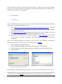
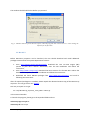
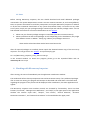
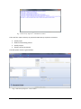
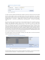
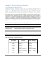
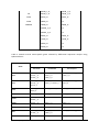
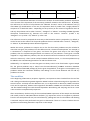
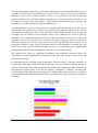
MICROARRAY INSPECTOR
Version 1.1.0.
User Manual
Warsaw 2013
Table of contents
Table of contents ................................................................................................................................. 2
1.
Application overview ................................................................................................................... 3
2.
System Requirements.................................................................................................................. 3
3.
Installation ................................................................................................................................... 4
4.
3.1
Windows .............................................................................................................................. 4
3.2
Mac OS X.............................................................................................................................. 5
3.3
Linux .................................................................................................................................... 6
Working with Microarray Inspector ............................................................................................ 6
4.1
Microarray Inspector Input ................................................................................................. 8
4.2
Definition of contaminating tissues .................................................................................... 8
4.3
Microarray Inspector Output ............................................................................................ 11
4.4
Microarray Inspector Control Parameters ........................................................................ 11
Appendix I – Microarray Inspector Algorithm ....................................................................................... 13
Overview and biomarker definition .................................................................................................. 13
The workflow ..................................................................................................................................... 15
Input parameters............................................................................................................................... 17
Tissues ........................................................................................................................................... 17
MAS5 parameters .......................................................................................................................... 17
Trimming Top and Bottom ............................................................................................................ 18
Significance level - α ...................................................................................................................... 18
References ..................................................................................................................................... 19
Appendix II – Microarray Inspector Charts in details ............................................................................ 20
Microarray Inspector User’s Manual
2
1. Application overview
Microarray Inspector is a bioinformatics tool developed by Transition Technologies, free for noncommercial and academic use. It is an application that uses statistical methods for a post-experiment
analysis of microarray experiments results to detect biological tissue contaminations.
DNA microarray is a powerful technique allowing for a simultaneous expression registration across
multiple genes. Quality assessment is one of the key issues in processing collected microarray data.
One aspect of microarray data quality control is ascertaining if the observed expression levels really
represent a given tissue or if they come from the presence of tissue-content contamination.
Contaminations in biological samples can appear due to insufficient isolation of the target cells from
surrounding tissues during the extraction process. Even relatively accurate methods of microdissection can be ineffective in protecting against contamination. Histopathology is a method that
can help to determine the degree of contamination of a sample. However, due to its invasive nature,
histopathology studies are not always performed.
In contrast to the invasive methods, Microarray Inspector allows the user to detect sample tissue
contamination via statistical methods. Contamination discovery in Microarray Inspector is based on
comparing the expression levels of known tissues’ biomarkers (sets of genes and/or probesets
supposedly specific to the given contamination) to the expression levels of the whole sample.
Alternatively, the comparison can be made between the biomarkers of the contaminant versus the
biomarkers of a reference tissue (supposedly the desired, uncontaminated tissue).
Current version of Microarray Inspector is prepared to handle microarray experiments in the
Affymetrix CEL format. If you are interested in using this software for other types of microarrays,
please contact us at [email protected].
To find out more about Microarray Inspector, download updates or read other information please
visit: http://bioinformatics.tt.com.pl
2. System Requirements
Microarray Inspector is a multiplatform Java application that can run on Microsoft Windows and
various Linux/Unix platforms, including Mac OS X. The application was tested on Microsoft Windows
XP/Vista/7 both in 32 and 64 bit versions, and Ubuntu 11, and Mac OS X 10.6.8 operating systems
and will probably work on the other Linux distributions as well. For full list of tested operating
systems, please visit our website (http://bioinformatics.tt.com.pl). Basic requirement to run the
program is Java run-time engine (JRE) version 6 or later.
Microarray Inspector uses some R libraries for preprocessing the microarray experimental results.
Because of this, the R environment, version 2.12.2 or later (http://www.r-project.org/), must be
installed as well.
Microarray Inspector User’s Manual
3
Finally, Microarray Inspector requires the LaTeX environment - pdflatex and a few other packages.
There are many ways to provide LaTeX support on different Operating Systems. Please refer to
installation section for the correct platform.
3. Installation
3.1 Windows
Before installing Microarray Inspector, the user should download and install additional packages
mentioned in the System Requirements section:
1. From http://www.oracle.com/technetwork/java/javase/downloads/index.html download
the Java run-time engine (JRE) specific to your platform. Afterwards, start the JRE installation
and follow the instructions.
2. From http://www.r-project.org/ download the latest version of R for Windows. When the
download is complete, start the R installation and follow the instructions.
3. Download the latest MiKTeX (2.7 or higher) package from http://miktex.org/ that is specific
to your version of Windows. Afterwards, install MiKTeX with all packages, following the
instructions.
After all the required packages are installed, the user can start the installation of Microarray
Inspector. Please obtain the newest copy of the installer from our website.
1.
2.
3.
4.
Start the Microarray Inspector installer.
Select the destination folder where the Microarray Inspector will be installed.
Select the Start Menu Folder where the shortcut to Microarray Inspector will be created.
Start installation.
Fig.1 Microarray Inspector® Installer
After installing, the Microarray Inspector is ready for use and can be started from the “Start” menu.
ATTENTION: when running the program for the first time, Windows XP users will be asked about the
access restrictions. Please deselect the default option “Run this program with restricted access”.
Microarray Inspector User’s Manual
4
The window should look like this before you proceed:
Fig. 2. Windows XP users please deselect option „Run this program with restricted access” when running the
software for the first time.
3.2 Mac OS X
Before Microarray Inspector can be launched, the user should download and install additional
packages mentioned in the System Requirements section:
1. From http://support.apple.com/downloads/ download the Java run-time engine (JRE)
specific to your OS X version. Afterwards, start the JRE installation and follow the
instructions.
2. From http://www.r-project.org/ download the latest version of R for Mac OS X. When the
download is complete, start the R installation and follow the instructions.
3. Download the latest MacTeX package from http://www.tug.org/mactex/ and install it
following the instructions.
After all required packages are installed, please unpack the obtained newest copy of the MicroArray
Inspector. You can get it from our website.
One way to unpack is to type:
tar –xvzf MicroArray_Inspector_Linux_OSX-1.1.0.tar.gz
in the terminal window.
To launch the program, please go to the unpacked folder and run:
microarray-app-1.1.0.jar or
microarray.sh start script.
Microarray Inspector User’s Manual
5
3.3 Linux
Before running Microarray Inspector, the user should download and install additional packages
mentioned in the System Requirements section: Java Run-time Environment, R, and LaTeX (pdflatex).
Next, we present commands to install the prerequisites and unpack MicroArray Inspector on Ubuntu
11.10, but the commands should work on any system from Debian family. To install it on any other
Linux system, simply use your package manager instead of apt and relevant package names. You can
find detailed instructions for more Linux distributions at our website.
1. Please use your favorite package manager to install JRE (Java Run-time Environment).
2. Please install basic R and LaTeX packages as well. Depending on the distribution, they might
have different names. In Debian - family (e.g. Ubuntu), the packages names are:
r-base texlive texlive-latex-base texlive-latex-extra latex-xcolor
After all required packages are installed, please unpack the obtained newest copy of the microarray
Inspector. You can get it from our website. To unpack simply type:
tar –xvzf MicroArray_Inspector_Linux_OSX-1.1.0.tar.gz
in the terminal window. To launch the program, please go to the unpacked folder and run
microarray.sh start script.
4. Working with Microarray Inspector
After starting, the user will immediately see the application initialization window.
The window will inform about prerequisites tests and environment setup. If any additional packages
of R or LaTeX are missing, the program will attempt to download and install them. The information
regarding the progress of the process will be displayed. After initialization, the main application will
appear.
The Microarray Inspector main window controls are clustered by functionality. There are three
buttons (“R Console”, “Manage Tissue Definitions”, and “Help”) in the upper panel of the application
window. The sections “Input Files”, “Output”, “Test Tissues”, “Control Selection”, “Presence
Detection Parameters”, and “Statistical Parameters” are located below the upper panel.
Microarray Inspector User’s Manual
6
Fig. 3. MicroArray Inspector® initialization window.
There are four steps necessary to prepare the Microarray Inspector to execute:




Specify input
Define contaminating tissues
Specify output
Specify control parameters
The description of each is given bellow.
Fig. 4. Microarray Inspector® main window
Microarray Inspector User’s Manual
7
4.1 Microarray Inspector Input
Fig. 5. CEL files input section
Detecting contaminations begins with specifying files containing microarray experiment results. Since
Microarray Inspector is only compatible with Affymetrix gene expression platforms, only .CEL files
should be provided. No other file formats are supported at the moment.
The “Input files” section contains a list of .CEL files used as input data. The buttons on the right side
from the list allows the user to configure the list of files.






“Add Files” button adds a selected .CEL file[s] to the input list
“Add Folder” button adds all .CEL files from a folder to the input list
“Move Up” button moves the selected .CEL file up on the input list
“Move Down” button moves the selected .CEL file down on the input list
“Remove” button removes the selected .CEL file from the input list
“Clear” button removes all .CEL files from the list
It should be noted that .CEL files in the list are not, by default, used in the analysis. For a file to be
used, it must first be selected / highlighted. To select all the files, click on a .CEL file in the list and
hold down the control key (command key on Macs) and press the ‘a’ key.
4.2 Definition of contaminating tissues
Microarray Inspector User’s Manual
8
Fig. 6. Test Tissues section
After specifying which .CEL files should be checked for contaminants, tissues that are to be
considered as possible contaminants need to be selected. This is done by using two lists in the “Test
Tissues” section. Initially, “Available tissues” list all currently defined tissues. “Test for presence of”
list will contain tissues to be investigated as possible contaminants in given .CEL files. Buttons
between the two lists allow the user to move defined tissues back and forth between the lists. Simply
put the tissues of interest in the “Test for presence of” list and Microarray Inspector will look for
them in the .CEL files.
In order to create a completely new tissue, the user should click the “Manage tissue definitions”
button on the application panel. This pops up the “Tissue Manage Window.” The left side contains a
list of all tissues currently defined, while the right side is divided into two sections intended for
specifying genes and probesets for tissues.
Fig. 7. Tissue Manage window
In order to proceed further, the user should understand the basic concept of how tissue presence
detection is implemented within the tool. Tissues in Microarray Inspector are sets of genes and/or
Microarray Inspector User’s Manual
9
probesets that should be specific to the given tissue (at least locally to where the sample was taken).
For example, adipose can be a possible contaminant in the study of breast cancer cells. The genes
signaling the contamination are commonly referred to as biomarkers or tissue-enriched genes (TEG),
and usually have significantly higher expression levels in DNA microarray experiments for a particular
type of tissue. Within microarray experiments, a single gene is represented by one or more
probesets. Furthermore, the mapping of gene symbols to probesets is platform (chip platform and
annotation platform) dependent. Therefore, the contaminant can be, in general, defined as a set of
gene symbols and a set of probesets.
Defining a new tissue in the “Tissue Manage Window” begins with entering the name of a tissue in
the “Tissue Name” field. Afterwards, gene and/or probeset symbols specific to the given tissue
should be selected. There are two ways to specify them. First, the user can define them by using the
“Define Gene” and “Define Probeset” fields, and clicking the appropriate “Add” button. Then the
respective gene/probeset appears in the “Selected Genes”/”Selected Probeset” list (if for any reason
you want to remove a user defined gene/probeset name from the database, highlight the item and
click on the appropriate “Remove” button). Secondly, the user can import all genes and probesets
from all the files listed as input in the “Input Files” section of the Main Window. User-defined genes
and probesets are written in bold and colored in blue within the lists; imported values are shown in
black. If a gene or probeset is at first user-defined but then found during the importation process, it
will not lose its status as user-defined. Other genes/probesets become associated with the new
tissue when their names appear in the “Selected Genes”/”Selected Probeset” list and the user saves
the tissue by clicking the “Add” button next to the “Tissues” list. The tissue name will appear in the
“Tissues” list. To commit any changes, the user should click on the “Save” button at the bottom of
the window; this closes the “Tissue Manage” window. Click the “Cancel” button in order to quit the
“Tissue Manage” window without saving any changes.
In order to edit a tissue, its name from the “Tissues” list needs to be selected when the user clicks the
“Edit” button. Genes/probesets associated with the selected tissue will appear in the “Selected
Genes”/”Selected Probesets” lists. Use the buttons marked with arrows between “Unselected
Genes”/”Unselected Probeset” and “Selected Genes”/”Selected Probeset” to move genes/probesets
between lists (a button with one arrow moves a selected genes/probesets, while a button with two
arrows moves all genes/probesets). When the “Selected Genes”/”Selected Probeset” list contains the
proper selection of genes/probesets which should be associated with the edited tissue, clicking the
“Add” button next to the “Tissues” list (the same one used in defining a new tissue) will save it to the
list. The user will be prompted to overwrite the tissue that already exists in the list. Clicking the
“Save” button at the bottom of the window will commit the changes and close the window. Clicking
the “Cancel” button will discard the changes and close the window.
In order to remove a tissue, select the tissue from the “Tissues” list and click on the “Remove” button
next to the “Tissues” list. Then click on the “Save” button and close the “Tissue Manage” window.
Click the “Cancel” button in order to quit the “Tissue Manage” window and discard the changes.
MicroArray Inspector comes with four tissue definitions. If these definitions were deleted during
usage of the program, the user can restore them by clicking “Restore default tissue database”. This
option overwrites irreversibly any tissues the user has defined and restores tissue database to fresh
installation state.
Microarray Inspector User’s Manual
10
4.3 Microarray Inspector Output
Fig. 8. Output Section
In order to select the folder where Microarray Inspector will write its output files, the user should
click the “Choose Folder” button in the Output section. The two other parameters in the “Output”
section allow to define how bar plots in the Microarray Inspector reports will be ordered. The
possible options are: “As listed” – displays bars on charts in the same order as they are given;
“Ascending order” – sorts bars in increasing order; “Descending order” – sorts bars in decreasing
order.
Microarray Inspector writes the output files in the specified location after successfully running its
analysis and generating reports. There will be two reports in form of PDF files
(ContaminationResults.pdf and PlatformDefinition.pdf), as well as an HTML file (index.html) with
charts in the specified output folder. The ContaminationResults.pdf file contains a summary of the
contamination decisions pertaining to each sample. The PlatformDefinition.pdf file contains technical
information about gene platforms, gene symbol to probeset mappings, and the parameters used in
the computations. The index.html file contains all the charts generated by Microarray Inspector along
with the summary information from the ContaminationResults.pdf report. Detailed description of the
charts is given the Appendix II “Microarray Inspector charts.”
The output directory will also hold folders containing raw output data in text files and pictures
divided in subfolders by tested tissue type.
4.4 Microarray Inspector Control Parameters
Fig. 9. Control Parameters in „Microarray Inspector”
The main window, where the user can specify the application parameters, consists of three sections:
“Presence Detection Parameters”, “Statistical Parameters”, and “Control Selection.”
Microarray Inspector User’s Manual
11
The “Presence Detection Parameters” section allows specifying the Affymetrix MAS 5.0 τ, α1, and α2
parameters. These parameters define thresholds on the sensitivity of the MAS 5.0 algorithm in
generating the “Present”, “Absent” or “Mismatch” detection calls.
The “Statistical Parameters” section is used to control and configure the reference probesets against
which the biomarkers are compared. The radio buttons “Primary control set” allow the user to select
which probesets of a given detection call (“Present”, “Marginal”, “Absent”) to use as a reference set
in the testing procedure. “Present” is the “strongest” condition because fewer samples will be
labeled as contaminated; “Absent” is the “weakest” in this sense. The significance level indicates how
strict the results are required to be. With a 0.0 significance level, we accept no results with 100%
confidence; with a 1.0 significance level, we accept all results with 0% confidence. In between these
two extremes, the user can define their own significance level. Refer to Appendix I for a detailed
discussion on the testing procedure. The “Trim Bottom” and “Trim Top” check boxes allow the user
to specify what reference probesets to ignore in the testing procedure defined by the extremes of
expression level.
Finally, in the section “Control Selection”, the radio button “Sample Whole Chip” allows the user to
decide if the testing procedure should be applied to the primary control set of the whole chip or all
the probesets (“Present”, “Marginal”, and “Absent”) of the given tissue.
Microarray Inspector User’s Manual
12
Appendix I – Microarray Inspector Algorithm
Overview and biomarker definition
The Microarray Inspector tool basically analyzes a set of the contaminant biomarkers against a
reference set. Technically, a biomarker is either a named gene - that will be mapped to a list of
probesets - or a named probeset. The contamination set is formed via a collection of probesets
mapped from each selected biomarker gene together with additionally selected biomarker
probesets. Provided predefined biomarkers are formed based on tissue specific and tissue-enriched
genes (TEGs). These genes are essentially expressed higher in the defined type of tissue[1, 2, 3]. So
the basis of a proper contamination analysis is a proper definition which tissues constitute the
contamination in a given microarray experiment, and which biomarkers are related to such tissues. It
is based on [1, 2, 3] the set of biomarkers proposed and tested in the context of the microarray
experiments in the field of oncology. This set was implemented in Microarray Inspector as a default
set. The result of the TEG genes analysis and a default biomarker set definition is presented in table 1
and 2.
Table 1. Possible tissue sample contamination in oncological experiments.
Cancer type
Possible contamination with
Breast cancer
Adipose, muscle, fibroblasts, vasculatory, or inflammation tissues
Colorectal cancer
Muscle, fibroblasts, vasculatory, or inflammation tissues
Ovulary cancer
Adipose, fibroblasts, vasculatory, or inflammation tissues
Eye cancer
Fibroblasts, vasculatory, or inflammation tissues
Brain cancer
Fibroblasts, vasculatory, or inflammation tissues
Table 2. Adipose tissue contamination biomarkers.
Biomarkers
(gene symbols)
Probesets platform HGU133plus2
Probesets platforms: HGU133A, HG-U133Av2
ADIPOQ
207175_at
207175_at
AQP7
206955_at
206955_at
CHRDL1
209763_at
209763_at
CIDEC
219398_at
219398_at
FABP4
203980_at, 235978_at
203980_at, 235978_at
ITH5
1553243_at, 219064_at
1553243_at, 219064_at
223828_s_at
N/A
LGALS12
Microarray Inspector User’s Manual
13
203548_s_at,
203549_s_at
203548_s_at,
203549_s_at
PLIN1
205913_at
205913_at
PLIN4
228409_at
N/A
SEMA3G
219689_at
219689_at
1554044_a_at
N/A
1558421_a_at
N/A
204997_at
204997_at
213706_at
213706_at
230463_at
N/A
231050_at
N/A
LPL
Table 3. Smooth muscle tissue-specific genes selected by differential expression analysis using
R/Bioconductor.
Probesets
Gene
HG-U133A
HG-U133Av2
HG-U133plus2
BGN
201261_x_at
201262_s_at
213905_x_at
201261_x_at
201262_s_at
213905_x_at
201261_x_at 201262_s_at
213905_x_at
FGF5
208378_x_at
210310_s_at
210311_at
208378_x_at
210310_s_at 210311_at
208378_x_at 210310_s_at
210311_at
IFFO1
209721_s_at
36030_at
209721_s_at36030_at
209721_s_at36030_at
COL1A1
202311_s_at
202311_s_at
202311_s_at
ITGA4
205884_at
205885_s_at
205884_at 205885_s_at
205884_at 205885_s_at
PRRX1
205991_s_at
205991_s_at
205991_s_at
ARHGAP22
206298_at
206298_at
206298_at
DCN
211813_x_at
211896_s_at
211813_x_at
211896_s_at
211813_x_at 211896_s_at
PAMR1
213661_at
213661_at
213661_at
Microarray Inspector User’s Manual
14
ELTD1
C1orf54
219134_at
219134_at
219134_at
219506_at
219506_at
219506_at
The
decision on contamination detection is based on the analysis of the biomarker probesets expression
in the context of the expression of the microarray probesets related to the reference set. By default,
the reference set consists of all probesets that obtained “Present” status in the Wilcoxon test [5]
after MAS5 [4] normalization. In this test, the expression level of probes from a single probeset is
compared to a threshold value τ. Depending on the p-values (in the context of significant level α1
and α2), the probeset can be either “Present”, “Marginal” or “Absent”. According to MAS5 algorithm
description nomenclature [4], decisions are made in this manner: “Present”: p-value ≤ α1;
“Marginal”: α1 < p-value < α2; “Absent”: p-value ≥ α2.
The reference set can be prepared the same way as the biomarker tissue is prepared or, by default, it
can be formed as the subset of all chip-wide probesets that are marked either “Present”, “Marginal”,
or “Absent” by the MAS5 presence detection algorithm.
Within the tissues, probesets are unique. Due to the fact that some probesets may be included in
more than one gene, the probesets’ list that defines tissue is cleaned from duplicates. For example, if
a contaminant is composed of five genes, and those five genes each map to the same single
probeset, then the contaminating biomarker set contains only one element. If each gene is instead
mapped to a single different probeset, then the set would contain five elements. Such uniqueness is
within the tissue only - there can be overlaps between different tissues, i.e. the same probesets may
be added to the contaminating biomarker set and the reference set.
Additionally, it is important to note that genes not always need to be found within a given sample
file; the gene-to-probeset map is taken from the Bioconductor[7] SYMBOL annotation database
available via AnnotationDbi package [6] for the given chip platform; if the gene is not mapped to any
probesets within the annotation database, then adding it to the tissue definition will not add any
probesets to the list.
The workflow
In the beginning of MicroArray Inspector algorithm, raw expression data is loaded from the .CEL files
and is being normalized using MAS5 algorithm. MAS5 has been selected among other algorithms for
several reasons. It already uses the Wilcoxon test, so it is adjusted for it. Moreover, MAS5 normalizes
each .CEL file separately, whereas other algorithms like RMA or GCRMA use information from all the
.CEL files loaded making the results dataset-dependent. Normalizing and analyzing one file at a time
is also much less computationally expensive.
After normalization, the base-2 log of the normalized MAS5 expressions of the sample are calculated
and initially scaled to 500 (Bioconductor defaults [7]). Expression values are mapped to probesets
from the two analyzed tissue sets (test and reference), yielding two lists of real numbers and allowing
a statistical analysis to be performed. Our goal is to determine if there is a reason to believe there is
significant contaminating biomarker expression in the sample.
Microarray Inspector User’s Manual
15
Next, the Mann-Whitney-Wilcoxon U Test is used to determine if the contaminating probesets are, as
a whole, less expressed than the reference set. There are two reasons to use the Mann-WhitneyWilcoxon U Test: the first, technical, reason is that it is a non-parametric test that can compare
datasets of different sizes. Secondly, and most importantly, it is a test that assesses whether one set
of numbers has larger values than another - exactly what we want when trying to compare the
expression of a possible contaminant against a reference set.
Our null hypothesis in this test is that the location (a pseudo-median) of the expression values of the
contamination set is greater than or equal to the location of the expression values of the reference
set; the alternative hypothesis then is, that the location of the expression values of the contaminant
is smaller than the location of the expression values of the reference set. The test yields no
information on the magnitude of the difference when the null hypothesis is rejected. If, with a given
significance level, the null hypothesis is not rejected for a given sample (i.e. we do not accept the
alternative hypothesis), then the sample will be marked as contaminated with the given set of
biomarkers. However, if with a given significance level the null hypothesis is rejected, then the
sample will not be marked contaminated with the given set of biomarkers; any contamination
determination is left to further investigation on the part of the involved scientists.
The statistical test relies on simplifying assumptions that probesets expression values are
independent and that the distributions of the two groups (test and reference) are the same, but
shifted from each other.
By implementing the described method, MicroArray Inspector allows a detailed inspection of
analyzed data. With each sample and each contaminant, it is easy to observe probeset expression
levels for all biomarker genes of the analyzed tissue. Each probeset additionally holds information of
the expression category which it was put to: “Present”, “Marginal” or “Absent”. The chart also
presents reference set expression by showing its first, second, and third quartile values. It enables a
relative estimation of the tested biomarkers versus the reference set. Figure 10 shows an example of
such chart.
Microarray Inspector User’s Manual
16
Fig. 10. Expression of single probesets defining biomarker genes. A – absent, M - marginal, P – present. Picture
also presents two first quartiles of reference set expressions.
In results of the MicroArray Inspector tool, there also is an easy to interpret box-and-whiskers chart.
It enables the comparison of distributions of each contaminant probeset expression for each sample.
Example is shown in Figure 11.
Fig. 11. Box-and-whiskers chart comparing gene expression distribution of the contaminant biomarkers to
reference sets.
The final output of the program is a report about tissue contamination in a PDF file, its Tex source,
and results in text versions.
Input parameters
Tissues
The MicroArray Inspector makes use of several parameters. Initially, the user should select which
experiment files (.CEL) to examine and what tissues to test for. The user can define their own
contaminant test tissues as a list of gene names and a list of probeset names; such names can be
imported from the current set of input .CEL files. Microarray Inspector comes with 4 predefined
biomarker tissues, but depending on the experiment, the user might want to detect other possible
contaminants. Providing this option was essential for assuring the tool’s flexible usage.
MAS5 parameters
The user can then specify the MAS5 Presence Detection parameters τ, α1 and α2, which are
described in the R documentation and have default values τ = 0.015, α1 = 0.04, α2 = 0.06. This will be
important for classifying the probesets as “Present”, “Marginal” or “Absent” by MAS5 and enables
the user to apply preferences dedicated to the experiment being tested.
Microarray Inspector User’s Manual
17
Next, the user should specify the reference set. First, the user should make a decision about the
control selection: either the tool will examine the whole chip for “Present”, “Marginal”, or “Absent”
probesets or a reference tissue will be used – in both approaches, a collection of expressions to test
the contaminants against will be formed for each sample. In forming such a set, the differences must
be noted between the choices. From the methods that use the presence detection results, using the
“Present” probesets imposes the strictest standards on marking a sample as contaminated. The
location (the aforementioned pseudo-median) of the expression of “Present” probesets will be
higher than that of “Marginal”, which itself will be higher than that of “Absent”. Hence, the
contaminant will have to be “more expressed” when tested against the “Present” probesets in order
to be marked as contaminated. Likewise, using the “Absent” probesets will eliminate most of the
samples as possibly contaminated. It may be desired by the user prefers to err on the side of caution,
and mark a good sample as bad rather than to let a bad sample be marked as good. When a
reference tissue is used, then the location of that reference tissue's expression is compared with that
of the contaminant tissue.
Trimming Top and Bottom
In addition to the selection of how to form the reference set, the user can further manipulate the set
by trimming data from the top and bottom of the expression values. Choosing to trim the top and
bottom values with an equal amount should not significantly affect the location of the reference set.
Trimming the top significantly more than the bottom should result in a reference set’s location with
lower expression values - and possibly more samples will be marked as contaminated. Trimming the
bottom significantly more than the top should result in a reference set’s location with higher
expression values - and possibly result in fewer samples being marked as contaminated. To be more
descriptive, trimming the top 50% of values will result in using the location as a pseudo first quartile
instead of a pseudo-median. Likewise, trimming the bottom 50% of values will result in using the
location as a pseudo third quartile instead of a pseudo-median.
Such flexibility in trimming is desired for some experiments. In some cases, even relatively low
expression of contaminant biomarkers can represent considerable contamination, while in other
cases it might be the opposite. Letting the user apply his expert knowledge to the analysis is the main
goal and concern behind this option. However, default settings should cover most of the cases.
Significance level - α
The final calculation parameter is the significance level α, which has a default value of 0.05. This is
the threshold that MicroArray Inspector will compare against the p-value returned by the MannWhitney-Wilcoxon U Test. The procedure runs as follows: Two groups of probesets from the sample
are formed - the contaminant and reference. As mentioned above, these groups are mapped to the
normalized expression values, and the Mann-Whitney-Wilcoxon U Test gives a p-value assessing
whether the numbers in the contaminant list are at least as large as those in the reference set. A
sample is marked as contaminated when such an idea - that the expression values from the
contaminant set are at least as large as those from the reference set – is not rejected. This happens
when the yielded p-value is greater than the significance level α. It can then be said that, with
(1-α)*100% confidence, the unmarked sample is not contaminated.
Microarray Inspector User’s Manual
18
Tuning α can easily loosen or tighten the analysis. Higher α will cause less samples to be marked as
contaminated, but the confidence of cleanliness estimation will drop. Smaller α yields more results
marked as contaminated but samples are estimated not to be contaminated with higher confidence.
References
[1] She X, Rohl CA, Castle JC, Kulkarni AV, Johnson JM, Chen R. Definition, conservation and
epigenetics of housekeeping and tissue-enriched genes. BMC Genomics. 2009 Jun 17;10:269
[2] Chunlei Wu, Camilo Orozco et al. BioGPS: an extensible and customizable portal for querying and
organizing gene annotation resources. Genome Biology 2009, 10:R130
[3] Sheng-Jian Xiao, Chi Zhang, Quan Zou and Zhi-Liang Ji, TiSGeD: a database for tissue-specific
genes. Bioinformatics (2010) 26 (9): 1273-1275.
[4] Affymetrix Statistical Algorithms Reference Guide
[5] Wilcoxon, F. Individual comparison by ranking methods. Biometrics 1, 80-83 (1945).
[6] Herve Pages, Marc Carlson, Seth Falcon and Nianhua Li. AnnotationDbi: Annotation Database
Interface. R package version 1.16.18.
[7] R. Gentleman, V. J. Carey, D. M. Bates, B.Bolstad, M. Dettling, S. Dudoit, B. Ellis, L. Gautier, Y. Ge,
and others, Bioconductor: Open software development for computational biology and
bioinformatics, 2004, Genome Biology, Vol. 5, R80
Microarray Inspector User’s Manual
19
Appendix II – Microarray Inspector Charts in details
Microarray Inspector reports contain four basic types of charts. The first forms the “High Level View”
and shows the application’s decision about contamination of the samples per tissue basis. Every .CEL
file on this chart is represented by a bar corresponding to the p-value computed during the
calculation procedure. Samples with computed p-values greater than the specified significance level
(contaminated) are shown in red. The samples with computed p-values smaller than the specified
significance level (not contaminated) are in green. The specified significance level is shown as a
vertical dashed line.
Fig. 12. Microarray Inspector® „High Level View” chart
The next type of chart forms is the “Detailed View” chart. In this type of a chart, the logged
expression levels for each probeset (organized by gene) comprising the biomarkers of the
contaminating tissue are shown for a given .CEL file. Each bar on the chart is marked with “P”, “M”,
or “A”, identifying the type of presence call (“Present”, “Mismatch”, “Absent”) produced by MAS 5.0
algorithm. Probesets representing the same gene have the same color. Finally, the 1st, 2nd, and 3rd
quartile of expression levels of the reference probesets’ are shown as vertical dashed lines (which
may be literally off the chart).
Microarray Inspector User’s Manual
20
Fig. 13. Microarray Inspector® „Detailed View” chart
The “Biomarker Expression” chart is the third type of chart produced by Microarray Inspector. This
chart does not work on expression data or p-value data, but rather on “meta-data” pertaining to
expression values. For a given sample and tissue, we show a box and whiskers view of the
distribution of its biomarkers among all the expressions for the whole sample. The bars are shown in
percentile values. For example, if a tissue consists only of probesets that are near the median of
expression level, then the chart would show a small bar centered around the 50% line. Again, these
are graphs of the percentage of the biomarker probesets to the entire chip.
Microarray Inspector User’s Manual
21
Fig. 14. Microarray Inspector® “Cross Sample Percentile View” chart
The graphs come with the following notes:
1. Let us refer to the percentiles of all the biomarker probesets as the q-data.
2. The values Q1 and Q3 represent the first and third quartiles of the q-data. They are not the
quartiles of the expression data - it is important not to confuse the two domains. 25% of all
q-data is less than the first quartile value; 75% of all q-data is less than the third quartile.
3. Let us refer to the value IQR=Q3-Q1 as an interquartile range.
4. Normal values are those that are within one and a half times the interquartile range from Q1
or Q3. To be more precise, a normal value is in the range between Q1 - 1.5 x IQR and Q3 + 1.5
x IQR.
5. Outliers are those values that are more than one and a half the interquartile range from a
value between Q1 and Q2. More succinctly, an outlier is a value less than Q1 - 1.5 x IQR or
greater than Q3 + 1.5 x IQR.
6. Outliers that are near one another are grouped together.
7. Two outliers next to one another indicate multiple outliers; a single outlier indicates a single
outlier.
8. The extreme markers do not indicate any specific value; instead, they indicate the presence
of outliers beyond twice the interquartile range from any interquartile value. More
succinctly, their presence indicates the values beyond the < Q1 - 2 x IQR ; Q3 + 2 x IQR >
range. These markers are used in place of all such values.
The last chart generated by Microarray Inspector is the “Test/Ref Expression” chart. The graph
presents a box-and-whiskers view of the expression of the tested tissue’s probesets vs. the
expression of the reference tissue’s probesets in each sample.
Microarray Inspector User’s Manual
22
Fig. 15. Microarray Inspector® “Cross-Sample Test vs. Reference Expression” chart
The graph comes with the following notes:
1. The values Q1 and Q3 represent the first and third quartile of the expression values. 25% of all
expression values is less than the first quartile; 75% of all expression values is less than the
third quartile.
2. Let us refer to the value IQR=Q3-Q1 as the interquartile range.
3. Normal values are those that are within one and a half times the interquartile range from Q1
or Q3. To be more precise, a normal value is in the range between Q1 - 1.5 x IQR and Q3 + 1.5
x IQR.
4. Outliers are those values that are more than one and a half the interquartile range from a
value between Q1 and Q2. More succinctly, an outlier is a value less than Q1 - 1.5 x IQR or
greater than Q3 + 1.5 x IQR.
5. Outliers that are near one another are grouped together.
6. Two outliers next to one another indicate multiple outliers; a single outlier indicates a single
outlier.
7. The extreme markers do not indicate any specific value; instead they indicate the presence of
outliers beyond twice the interquartile range from any interquartile value. More succinctly,
their presence indicates the values beyond the < Q1 - 2 x IQR ; Q3 + 2 x IQR > range. These
markers are used in place of all such values.
Microarray Inspector User’s Manual
23