Download Mehiar Moukbel

MBVC – Model Based Version Control:
An Application of Configuration
Management on Graphical Models
MEHIAR MOUKBEL
Master of Science Thesis
Stockholm, Sweden 2007
i
MBVC – Model Based Version Control:
An Application of Configuration Management on
Graphical Models
By:
Mehiar Moukbel
A
Merge
Engine
AB
B
Master of Science Thesis MMK 2007:38 MDA261
KTH Machine Design
SE-10044STOCKHOLM
ii
Master of Science Thesis MMK 2007:38 MDA261
MBVC – Model Based Version Control:
An Application of Configuration Management on
Graphical Models
Mehiar Moukbel
Approved
Examiner
Supervisor
2007-03-20
Martin Törngren
Jianlin Shi
Jad El-Khoury
Commissioner
Contact person
KTH, Machine Design
Abstract
File-based version control consists of tools in the software engineering industry, with
many available commercial products that allow multiple developers to work
simultaneously on a single project. However these tools are most commonly used on
plain textual documents such as source code.
There exist few tools today for versioning fine-grained data such as graphical Simulink
models. Since Simulink is widely used as a modeling tool in numerous engineering
fields, nonetheless in the mechatronics field, it will be interesting to study the possibility
of developing a tool for version control of graphical models.
Two textual software configuration management (SCM) products, CVS and Rational
Clear Case, were studied and their functionalities were analyzed, along with a different
number of research topics on document versioning. The existing algorithms of ‘diff’ and
‘merge’ functions were also studied to give an understanding of how these functions
work for text based documents. The knowledge gained from the tools, existing
algorithms and literature on the subject were used to write MATLAB programs that
perform diff and merge on Simulink models.
The resulted programs perform 2-way diff and merge on Simulink models and display
the differences graphically using color codes. Although the tool did have some
limitations and did not perform all the expected SCM functions, it still displayed
differences between Simulink models. Displaying of results occurred both graphically
and textually. A third tool called Rhapsody was studied which is used in model driven
development and its interaction with Simulink was also studied, showing that is possible
but rather complex and requires knowledge in both programs.
The study shows thus that it is possible to build and develop configuration management
tools for graphical models in Simulink, possibly also the 3-way merges, but certain
difficulties such as connecting blocks correctly must firstly be solved.
iii
Examensarbete MMK 2007:38 MDA261
MBVC – Versionshantering av Grafiska
Modeller
En Applikation av CM
Mehiar Moukbel
Godkänt
Examinator
Handledare
2007-03-20
Martin Törngren
Jianlin Shi
Jad El-Khoury
Uppdragsgivare
Kontaktperson
KTH, Maskinkonstruktion
Sammanfattning
Filbaserad versionshantering är ett verktyg inom mjukvaruutvecklingen, och det
existerar ett stort utbud av kommersiella produkter. Problemet är dock att de flesta
verktygen fungerar endast för textbaserade filer, och saknar någon motsvarighet till
hantering av ’fine grained’ filer som exemplevis grafiska Simulink modeller. Eftersom
Simulink är ett utspritt modelleringsvertyg och används inom flera utvecklingsarbeten
och särskillt inom mekatronik, så är det intressant att studera möjligheten att utveckla ett
sådant verktyg.
Genom analys av två tillgängliga konfigurationsverktyg: CVS och Rational Clear Case,
samt studie av diverse publikationer och rapporter av versionshantering och algoritmer
angående ’diff’ och ’merge’ funktioner, så utvecklades ett enkelt sådant verktyg.
Programmet utför enkel skillnads- och föreneingsfunktioner (2-way merge) på grafiska
Simulink modeller. Verktyget fungerade inte som det var uttänkt i början men det
lyckades ändå visa skillnader mellan Simulink modellerna både grafiskt och
textmässigt. Ett tredje verktyg, Rhapsody, som används inom MDD studerades, samt
dess samarbete med Simulnik testades. Resultatet visar att programmens samverkan är
möjlig men något komplex och kräver erfarenheter från båda programmen.
Studien visar att det går att bygga ett mer avancerat konfigurations-hanteringsprogram
för Simulink modeller, såsom ett 3-way merge, men vissa svårigheter som en korretk
koppling av blocken måste först lösas.
.
iv
Model Based Version Control – An Application of Configuration Management on
Graphical Models
Keywords
Model based version control, MBVC
Software Configuration Management
Configuration Management
CVS / Clear Case
Difference, diff
Merge, 2-way merge, 3-way merge
Abbreviations
The following is a list of all the abbreviations used in this report.
API: Application Programming Interface
CC: Clear Case
CM: Configuration Management
CVS: Concurrent Versions Systems
MDD: Model Driven Development
MDA: Model Driven Architecture
RCS: Revision Control Systems
RG: Rhapsody Gateway
SCM: Software Configuration Management
SE: Software Engineering
STEP: STandard for the Exchange of Product model data
PDM: Product Data Management
UBCC: Usefulness Based Control Code
UML: Unified Modeling Language
VCS: Version Control System
VOB: Version Object Base
XML: eXtensible Markup Language
v
Model Based Version Control – An Application of Configuration Management on
Graphical Models
Contents
1 Introduction.................................................................................................................1
1.1 Background and Introduction................................................................................1
1.2 Problem..................................................................................................................2
1.3 Goal .......................................................................................................................2
1.4 Approach................................................................................................................2
1.5 Assumptions and Limitations.................................................................................3
1.6 Thesis Outline ........................................................................................................3
2 SCM and Model Based Development........................................................................5
2.1 Basics of SCM........................................................................................................6
2.1.1 SCM Workflow...................................................................................................................... 7
2.1.2 The Repository....................................................................................................................... 7
2.2 Model Driven Development ...................................................................................7
2.3 Summary of Chapter 2:..........................................................................................8
3 Existing Software Configuration Management Tools .............................................9
3.1 CVS ........................................................................................................................9
3.1.1
3.1.2
3.1.3
3.1.4
3.1.5
The CVS Repository............................................................................................................10
Viewing Differences ............................................................................................................11
Revisions ..............................................................................................................................11
Branching and Merging .......................................................................................................12
Multiple Developers ............................................................................................................13
3.2 Rational Clear Case ............................................................................................13
3.2.1
3.2.2
3.2.3
3.2.4
ClearCase Views..................................................................................................................13
Versions, Elements and VOBs ............................................................................................14
Checking Out Files ..............................................................................................................14
Checking In Files .................................................................................................................15
3.3 Rhapsody and the Telelogic Family ....................................................................16
3.3.1
3.3.2
3.3.3
3.3.4
3.3.5
Short about UML 2.0 ...........................................................................................................16
The Rhapsody GUI ..............................................................................................................17
Rhapsody in C++ .................................................................................................................17
More Telelogic Programs ....................................................................................................19
Conclusions Regarding Rhapsody.......................................................................................20
3.4 Summary of the SCM Tools .................................................................................21
3.4.1
3.4.2
3.4.3
3.4.4
Concurrent Development.....................................................................................................21
The Diff................................................................................................................................22
The Merge ............................................................................................................................22
Locking-Unlocking the Model ............................................................................................23
4 The Analysis of Existing Algorithms: Flat vs. Hierarchic ....................................25
4.1 Diff Algorithm for Flat Data................................................................................25
4.1.1 Longest Common Subsequence...........................................................................................26
4.1.2 Representing the Differences...............................................................................................28
4.1.3 2-way vs. 3-way Difference: Presenting the Differences ...................................................28
4.2 Merge Algorithm for Flat Data ...........................................................................29
4.2.1 Definition of Merge .............................................................................................................29
4.2.2 The 3-way Merge.................................................................................................................30
4.2.3 Merge: Relationship to the Difference ................................................................................34
4.3 Diff Algorithm for Hierarchical Data..................................................................34
4.3.1
4.3.2
4.3.3
4.3.4
The XML Language.............................................................................................................34
The Theory of XML Document Versioning .......................................................................36
Edit operations .....................................................................................................................38
Edit Scripts: Cost Models ....................................................................................................40
4.4 Merge Algorithm for Hierarchical Data .............................................................40
vi
Model Based Version Control – An Application of Configuration Management on
Graphical Models
4.5 Summary of Chapter 4 .........................................................................................41
5 The Desired Tool Specifications ..............................................................................42
5.1 Considerations for the Model Based Approach...................................................42
5.1.1 The Input and Output Types................................................................................................43
5.1.2 Colour Scheme.....................................................................................................................43
5.1.3 Limitation.............................................................................................................................43
5.2 Desired Use Case of the ‘Difference’ Program ..................................................43
5.3 Desired Use Case of the Merge Program............................................................44
5.4 Summary of Chapter 5 .........................................................................................44
6 Implementation of Model Based Tool.....................................................................45
6.1 The Input and Output Models ..............................................................................45
6.2 Actual ‘Diff’ Program..........................................................................................45
6.2.1
6.2.2
6.2.3
6.2.4
6.2.5
Modules................................................................................................................................45
‘Difference’ Algorithm ........................................................................................................46
Displaying the Differences ..................................................................................................48
Actual Results: Difference...................................................................................................49
What Did Not Work: Diff....................................................................................................51
6.3 Actual Merge Program ........................................................................................51
6.3.1
6.3.2
6.3.3
6.3.4
6.3.5
Merge Modules ....................................................................................................................52
Merge Algorithm .................................................................................................................52
Displaying the Differences: Merge .....................................................................................54
Actual Results: Merge .........................................................................................................55
What Did Not Work: Merge................................................................................................55
6.4 Summary of Chapter 6 .........................................................................................55
7 Simulink and Rhapsody ...........................................................................................57
7.1 Simulink and Rhapsody........................................................................................57
7.2 Vertical Integration Using Rhapsody Gateway and Traceability .......................57
7.3 Horizontal Integration Workflow ........................................................................59
7.3.1 Other Workflow Methods....................................................................................................60
7.4 Summary of Chapter 7 .........................................................................................61
8 Conclusions and Discussions....................................................................................62
8.1 Conclusions..........................................................................................................62
8.2 Discussions ..........................................................................................................63
8.3 Future Work.........................................................................................................64
References: .....................................................................................................................65
Appendix: .......................................................................................................................70
vii
Model Based Version Control – An Application of Configuration Management on
Graphical Models
1 Introduction
1.1 Background and Introduction
This thesis was performed at the Mechatronics Department at the Royal Institute of
Technology in Stockholm, Sweden 2005-2006.
The implementation of version control in software engineering has been a contributing
factor to the evolution and rapid development of new and advanced software products.
The most obvious advantage of such system lies in its ability of allowing multiple users
to work simultaneously on the same data, to finally allow merging the finished result in
a clever fashion that otherwise, without version control, would lead to confusion and
loss of efficiency.
Traditional software configuration management (SCM) tools are used for managing
code source and text files also known as plain files. This paper will discuss and show
the possibility of applying the configuration management (CM) on graphical models
known as hierarchical or fine grained data such as Simulink models. This type of file
differs from the plain files in the sense that the structure of the data has semantics.
The initial stages of a version control system (VCS) for models have been established
by Jad El-Khoury1. To make the system more similar to an SCM tool for graphical
models, it has to be supplemented with features common in standard SCM tools, such as
the diff and merge functions.
The most common functionalities that are applied in SCM tools today are merging,
branching, checking out files (two options available: either reserved or unreserved
checkouts), updating and differencing (viewing differences between two versions of the
same file). The functionalities will be described in more detail in the sections that
follow.
MDD (Model Driven Development) is an approach that refers to the usage of models as
the main engineering artifacts and is considered as the primary class entities in an
engineering lifecycle. The term MDD is considered generic, and MDA (Model Driven
Architecture) is a specific term belonging to the Object Management Group (OMG).
MDA consists of a platform independent base model along with one or more platform
specific models, including sets of interface definitions each describing how to
implement the base model on different middleware platforms. [OMG]
Traditional development of software involved coding at an early stage by software
engineers, where they had to continuously debug, test and run code throughout the
development stage. If any changes were to be made at a later stage in the program life
cycle, then huge efforts had to be put on even more testing and debugging.
Rhapsody, which is the tool tested in this paper, is based on the MDD technology.
Systems are modeled in MDD using UML 2.0 models. The effort is put on the system at
1
Jad El-Khoury, PhD at mechatronics Department, KTH
1
Model Based Version Control – An Application of Configuration Management on
Graphical Models
an abstract level, while less effort is put on the coding, since one of Rhapsody’s
functions is to generate embedded code.
1.2 Problem
The problem is how to use the knowledge from existing algorithms and tools that apply
SCM on text files, to transform it and apply it on Simulink models. The first problem
encountered was that the structure of text documents differs from graphical models.
How does one relate a sentence in a page to a Simulink block in a model? Does
MATLAB support functions that allow building of such programs?
1.3 Goal
There are two goals concerning this thesis. The first goal of is to develop ‘diff’ and
merge functions to be applied on Simulink models. The user will enter two Simulink
models and the program will produce an output model that will contain the differences
of the two input models. The results will be shown both graphically and textually. A
merge will also ask the user when conflicts occur: which block coming from each
revision to be merged.
The second goal is to test how Rhapsody interacts with Simulink models and try to
understand the possibilities and capabilities supported by them and sum up the
experience.
1.4 Approach
To achieve the first objective of this thesis, topics on plain and fine-grained data were
studied, which gave an understanding of the plain and fine-grained structure. Then the
existing diff and merge functions were studied to give a basic understanding on how
they work. This included white papers and theoretical studies on the diff. Thereafter two
SCM tools, CVS and Clear Case, were studied and their functionalities were analyzed.
This gave a broader understanding on the capabilities of the tools, and showed what was
possible to perform using them. It also gave an understanding on how the tools are
activated, specifically CVS because it uses a textual user command interface.
Then more research was performed on the diff and merge functions of the SCM tools by
studying white papers on the algorithms of these two functionalities. Thereafter the
programming methodology of MATLAB was studied and specifically the functions
used with Simulink models. This gave a picture of what functions were useful, and also
a better understanding of the layout and structure of Simulink models. The property of
Simulink was then studied, and this showed the properties which blocks were made up
of.
The information gained was then used to derive a method for performing diff and merge
on Simulink models, by using the information gained from the block properties and by
applying algorithms developed from existing tools and other theoretical information of
the current diff applied to textual documents.
2
Model Based Version Control – An Application of Configuration Management on
Graphical Models
The second objective: to study how well Rhapsody and Simulink interact together, and
look on the MDD approach. Rhapsody was installed and tested to understand its
capabilities. Moreover, white papers covering Rhapsody were studied, webinars, which
are seminars via the web, were attended and different instructional videos were
watched. Built-in tutorials of Rhapsody were also used to gain deeper insight of the
capability of the software, and UML 2.0 was also revised. MDD and MDA were also
studied.
1.5 Assumptions and Limitations
Some assumptions have been made regarding the size and complexity of the models. In
the textual approach, files containing thousands of lines are common when the
algorithms are applied for the difference and merge programs. This results in different
algorithms having different levels of time complexities and efficiencies. In this thesis
however the complexity of the algorithms has not been taken into account, since that
was not the main aim of the project.
Secondly the Simulink models are regarded as multi-nodes and quite complex with the
respect to the sub-system blocks. The structure of the models will be more thoroughly
explained in the API of MATLAB section. A complete MBVC or Model Based Version
Control system consists of two main parts: the system for checking in and out files, plus
the ability to perform different changes to the files such as finding differences and
merging them. It is the latter part that will be developed in this thesis.
The algorithms of the two functions that were studied, the difference and merge
functions will not be exactly translated into the model based approach. The textual
system will thus rather act as a base for understanding the logic and theory behind the
algorithms that will be applied to the fine grained graphical models.
The systems that were developed have been tested for the most commonly used toolbox,
and was not tested with other more complex toolboxes, but the logic of the program was
written to be independent of the type of blocks being used.
The student version of MATLAB being used handles models with a maximum of 1000
blocks, so although models of these sizes are used in real engineering projects, they
were not tested in this thesis, since the complexity of the algorithms was not taken into
account.
The mathematical approach of the algorithms chapter will not be implemented when
developing the actual programs. These approaches were studied to get a broader
understanding on how complex and real algorithms in the market work, and what degree
of complexity they implement.
1.6 Thesis Outline
Chapter 2 talks about the two major engineering development approaches: SCM and
MDD, and about their major characteristics. The history of how the diff began is
introduced.
3
Model Based Version Control – An Application of Configuration Management on
Graphical Models
In chapter 3 existing SCM and MDD tools are discussed and the general functions
provided along with their capability. The tools are CVS, Clear Case and Rhapsody.
Thereafter current algorithms behind the merge and diff functions are summed up using
a mathematical approach in chapter 4. Both the plain and fine grained algorithms are
discussed.
Chapter 5 discusses the desired algorithms for the diff and merge and discusses both the
requirements on the input and output formats and coloring system as well as the desired
use cases.
In the next chapter, chapter 6, the actual diff and merge programs, that was developed as
a result of the previous chapters, are described and discussed. They also contain the
actual algorithms and pictures from the resulting programs.
Chapter 7 consists of a study on Rhapsody which is a MDD modeling program. There
are also two different ways of combining it with Simulink models: horizontal and
vertical merging. The final chapter 8 is the conclusions and discussion that are reflected
upon the entire project and some possible future work.
4
Model Based Version Control – An Application of Configuration Management on
Graphical Models
2 SCM and Model Based Development
A large number of SCM systems and concepts are available today. There are two main
types of data structures: the plain and fine grained. The main difference between them
being that the latter involves semantics of the documents and thus introduces logic into
the document.
However most SCM tools only work with plain files, which are files containing lines of
printed text. There are few configuration management systems that manage hierarchical
data structures and tree data systems, such as those present in the XML language. Thus
it is important to understand that most SCM tools treat text files as pages with printed
text, without taking the logic of the files’ structure and content into consideration. This
introduces a problem in working with graphical models because they contain important
semantics that are not included in plain text files. [CON]
This thesis will consider the development of a model based development tool since it
will handle performing diff and merge operations on Simulink models. These models
take the semantics into consideration and are thus of fine grained or hierarchical nature.
The classical method in developing technical systems has been to use paper and pen to
sketch the initial layout of the system. The requirements were then taken into account
and these would be the basis for the development engineers whose work would involve
coding by hand. This was a long and challenging process and required an early and
accurate definition of the problem to be able to formulate a solution. Thus each coded
function would have multiple arguments and would produce different outputs, a process
that was interconnected, and where a change in any requirement at a later stage would
imply huge loss in efficiency because all the code had to be reviewed and updated
manually.
Newer development solutions employ a new approach known as MDD. One such
program is Rhapsody and it uses the UML 2.0 modelling language. Rhapsody allows
the user to model the project in the UML language and keep track using traceability of
the components and requirements using add-ons. The user can then generate code to be
directly implemented into embedded systems. One advantage is that Rhapsody can
interact with other programs such as Simulink in different ways.
The problem is then to connect Rhapsody and Simulink so that data exchange can occur
between them. This is done by one of two methods: either using an external program or
using built-in functions of both programs to achieve the communication. An example of
an external program is Rhapsody Gateway which is used to create traceability links
across the models and requirements. The second major method is to use the internal
functions that allow the import of generated code from the program. More about this is
discussed in chapter 7 about relating Simulink and Rhapsody.
A number of different studies and research topics covering version management, fine
grained version control, XML version management, and the basic principles of SCM
such as [CHIEN], [HAU], [CON], [CHAW] were studied. Algorithms proposed for the
difference and merge methods were also studied and analyzed.
5
Model Based Version Control – An Application of Configuration Management on
Graphical Models
Version control systems cover a large topic in modern configuration management tools,
and in this thesis it will be known as the model based version control or MBVC, since it
is about managing revisions of graphical models. A MBVC tool consists of two main
scopes:
•
•
Repository: a server/client approach for storing and retrieving the data, to make
it available for others, either located in the same office room or in another
continent
Functionalities: different functionalities that are applied to the data, such as
merging and differencing the data.
2.1 Basics of SCM
SCM is a management tool that applies an engineering discipline to manage and control
the evolution of complex software systems or more practically expressed, it is the
discipline that enables one to keep evolving software products under control, and thus
contributes to satisfying quality and delaying constraints [EST]. The primary focus of
this discipline is to ensure repeatability, traceability and integrity of the system being
developed and produced. Today, SCM is a well established and common practice in the
later phases of software development, more notably during programming and
integration. [OHST], [BOB]
The diff was originally developed in the early 1970’s for the UNIX systems which was
developed at the AT&T Bell Labs. An initial but rather unreliable program known as
proof was written by Steve Johnson. It was considered as unreliable because it produced
line by line changes and used angle brackets (< and >) for presenting line deletions and
line insertions. A final and more reliable program that is still in use today, the diff, was
written by Douglas McIlroy for the early UNIX systems. His research study was
published in 1976. This program is still considered as the mother of the modern
configuration management differencing tool, although there has been significant
improvements on the algorithms and speed of the processes for handling larger text
documents.
SCM emerged as a discipline soon after the software crisis during the late 70’s and early
80’s, when it was understood that programming is not the sole factor for success in
Software Engineering (SE), as other factors such as architectural development and
evolution play a vital role for achieving advances in SE. At the time it was developed,
SCM was considered more of as a version management and rebuilding tool, while
nowadays the typical configuration management system aims to provide a wider
perspective, covering important topics such as process support, concurrent engineering
and distributed development.
There are many tools available on the market today, and they all tend to provide the
following basic features: (1) place to store the source code; (2) provide a historical
record over what has been done over time; (3) provide a method for different developers
to work on the same project simultaneously and merge their work; (4) the developers
can cooperate without getting in the way of each other. [SINK]
6
Model Based Version Control – An Application of Configuration Management on
Graphical Models
2.1.1 SCM Workflow
SCM tools generally employ the following workflow:
1- The user copies the file from the repository into a working directory: this is done
so that there will always exist original documents that can be reviewed later on
in the future.
2- The user applies the changes to the file in the working directory: so that no two
users can overwrite each others work, and this allows place for individual
creativity and concurrency.
3- The updated files are returned into the repository with a new version number: so
that each document has its own identity of who created it and when it was
created. This step may require a merge to be applied.
4- The above steps are repeated for the entire project.
Each different program applies a different syntax, and uses different nomenclature for
the different steps, but the idea is basically the same.
2.1.2 The Repository
A repository is the place where all data files are stored, available for all users in a
certain project. The directories and files are arranged in a tree file system, but the
special about this configuration is that it involves a third dimension, namely time.
The repository keeps a track record of every change that has ever been made to all files
and directories, as well as who did what and when. The system does not store all new
revised files as it would require huge amounts of disk space. Thus the system stores the
changes that are made, known as deltas, or differences between the latest checked in
model and the model that is currently being checked in.
2.2 Model Driven Development
The expression MDD stands for a concept where the development of projects is initiated
from the model and allows engineers to overview the model in an abstract and objective
way, compared to viewing the project entirely as code. In Rhapsody this gives
developers a UML model in the early development stage, and as work proceeds, the
model, the functions and events can be monitored and tested throughout the
development process. Tools such as Rhapsody allow for production of code for the
embedded target system.
By comparing this approach to the classical approach it is evident that changes can be
easily made and monitored, and any new project requirements are integrated and traced
into the project. Otherwise it would be necessary to manually check for changes after
project initiation and make sure that no errors will be made, making it difficult to trace
the new changes, and perform more testing and debugging throughout the development
life cycle.
Another important advantage behind this system architecture lies in the fact that the
final product is binary executable. This means it can be run on an embedded target with
a real time operating system, without the need of re-testing or modifying the model.
[NIE]
7
Model Based Version Control – An Application of Configuration Management on
Graphical Models
The disadvantages that can bee seen are the time and money needed to learn and invest
into a new software package along with the UML language. Another would be the sole
dependency on one product that performs a wide and important task such as developing
an entire project. And finally it is important to understand the nature of the embedded
system in terms of its storage capacity and processing speed
2.3 Summary of Chapter 2:
SCM is a wide and interesting topic which is considered important in the development
of new software. The advantage of it lies in the fact that it introduces powerful functions
that allow multiple users to work on the same project at the same time. It started of with
the development of the diff function by Douglas McIlroy back in the 1970’s. All SCM
tools have a repository that contains all the data which allows users to check out the
data, edit it and check it back in. The user has the option to perform diff and merge
operations on the files to keep track of what changes that have been made and support
concurrent development.
The data consists of two main types: plain and fine grained data. There is an important
difference between them: their semantics. Plain data consists of printed lines of
characters and text. When looking for differences between two plain data file only the
actual letters or lines that have been edited, added or deleted will be considered. The
data content is not considered only its layout.
For example by moving a function in C code to a different place in the document, the
program will behave exactly the same, but by performing a diff the user will get huge
differences: the addition of the entire function at its new location and the presence of its
old location in the previous version. So the SCM tool will display differences and any
developer wanting to work on the file must perform a merge, while in reality there
should be no need for it since the two C files perform exactly the same function. This
occurs because source code documents do not contain semantics.
In the fine grained data, such as XML and UML, the semantics are of importance. That
means the data content and its syntax is taken into consideration when searching for
differences. For example: representing a library structure in XML with book tags, and
where each book contains attributes such as author and title. Changing the location of a
book and its content on XML would change its physical layout, but its contents are the
same.
The advantage of using fine grained data lies in its ability to represent more information
than can be presented by plain data files making it more powerful. It allows for faster
development since only the data content is of importance and not the layout, thus
allowing for facilitated change management.
8
Model Based Version Control – An Application of Configuration Management on
Graphical Models
3 Existing Software Configuration Management Tools
The goal of the first two subchapters is to introduce and describe two common SCM
tools that are widely used today in development projects. This will give an overview of
the general structure of the programs, and show the possibilities that exist for common
SCM tools. By showing sample sessions and examples of common functions one can
better understand the general structure of the programs and their syntaxes. In the third
subchapter Rhapsody is introduced which is a tool used in the MDD approach.
3.1 CVS
The following chapter is a taken from the manual of the CVS software, [CED], and
describes the usage and syntax of CVS, a common and popular version control system.
Concurrent Versions Systems or CVS is a version control system used to record the
history of source files. With CVS the user can easily retrieve old versions of documents
to (for example) see exactly which change in a certain document caused a bug. CVS
stores all the versions of a file in a single file in a way that only stores the difference
between versions, known as deltas, instead of storing all the versions which would
otherwise waste disk space.
CVS becomes also helpful when multiple users work on the same project, thus the name
Concurrent in CVS, and share the same data resources. As the size of the group grows,
it becomes easier to overwrite each others’ changes, resulting in loss of project data and
efficiency. CVS avoids this common problem by insulating the different developers
from each other. Every developer works in his own directory and CVS merges the work
when each developer is done with his or her work. This is achieved by checking out the
files, performing changes and then checking them back into a common repository.
• What CVS does not represent
The following is a list of six points that CVS does not represent. This will explain what
CVS is capable of doing for its user, and what it is not capable of doing:
1. CVS is not a build system: CVS does not dictate how to build anything, it
merely stores files for retrieval in a tree structure which the user devises.
2. CVS is not a substitute for management: the project leaders will still have to
keep frequent meetings with the engineers and make them aware of the projects’
current status and progress.
3. CVS is not a substitute for developer communication: when a developer comes
across a conflict which is too difficult to solve on his own, he will have to solve
it by communicating with other developers.
4. CVS does not have change control: the program does not keep track of all the
bugs and status of each of them.
5. CVS is not an automated testing program: the software will not perform
continuous tests on the written code; it is up to the user to keep track of such
activities.
9
Model Based Version Control – An Application of Configuration Management on
Graphical Models
6. CVS does not have a built-in process model: the system does not provide ways
to ensure that changes or releases go through various steps, with various
approvals as needed.
3.1.1 The CVS Repository
The CVS repository stores a complete copy of all the files and directories which are
under version control. The files in the repository are never directly accessed, instead one
uses CVS commands to get a copy of the files into a personal working directory
(sandbox), and then work on that directory. When finished modifying the files the user
checks or commits them back into the repository. The repository will now contain the
changes made, when they were made and by whom.
• A Sample Session
The following is an example of a sample session which describes basic commands that
are often used when initially applying CVS to a file. Suppose one is working on a
compiler and the source consists of a handful of C files and a ‘Makefile’. The compiler
is called ‘tc’ (Trivial Compiler), and the repository is set up so that there is a module
called ‘tc’.
CVS stores all files in a centralized repository, also known as the vault. First the user
must get a working copy of the source for ‘tc’, achieved by using the ‘checkout’
command:
$ CVS checkout tc
This will create a new directory called ‘tc’ and populate it with the source files.
Suppose one of the files is ‘backend.c’ and that the user performs some changes to that
file and want to save the new version in the repository, making it available to anyone
else who is using that same repository:
$ CVS commit backend.c
CVS will start an editor to allow one to enter a log message (for example: “Added an
optimization pass”). The launch of the editor can be avoided by using the ‘-m’ flag:
$ CVS commit –m “Added an optimization pass” backend.c
• Cleaning Up
Before exiting the session, the user will remove the working copy of ‘tc’. This is
achieved by:
$ CVS release –d tc
The ‘-d’ flag removes ones’ own working copy.
10
Model Based Version Control – An Application of Configuration Management on
Graphical Models
3.1.2 Viewing Differences
If a user does not remember having modified a certain file, the changes can be viewed
by using the ‘diff’ command. For checking on the file ‘driver.c’:
$ CVS diff driver.c
The ‘diff’ command will compare the version of the working copy with the one that
was checked out, and print the changes that have been made.
• Starting a Project with CVS
For a new project, the easiest method is to start by creating an empty directory structure.
In the following: one main directory, ‘tc’, with the two subdirectories ‘man’ and
‘testing’ are created
$ mkdir tc
$ mkdir tc/man
$ mkdir tc/testing
After using the ‘import’ command to create the corresponding empty directory
structure inside the repository:
$ cd tc
$ cvs import –m “Created directory structure”
yoyodyne/dir
yoyo
start
This will add yoyodyne/dir as a directory under $CVSROOT. Then use ‘add’ to add new
files and new directories as they appear.
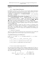
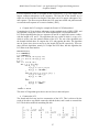
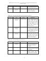
3.1.3 Revisions
If one wants to keep track of a set of revisions, also known as versions, involving more
than one file, such as which revisions went into a particular release, one easily employs
a tag. A tag is a symbolic revision which can be assigned to a numeric revision in each
file.
The ‘checkout’ command has a ‘-r’ flag that lets the user check out a certain revision
of a module. Deleting and moving tags is a dangerous act, which permanently discards
historical information and makes it difficult or impossible to recover from errors. Thus
care must be taken when moving or deleting the tags.
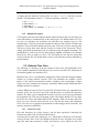
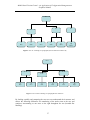
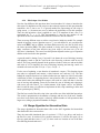
The following figure illustrates the usage of tags:
File 1
file 2
file 3
1.1
1.1
1.1
1.2*\
1.2
1.2
1.3 \--- 1.3*-\ 1.3 /
1.4
\ 1.4 /
\--1.5*1.6
file 4
file 5
1.1 /--1.1*
-1.2*--/
1.3
1.4
1.5
11
Å* --Tag
Model Based Version Control – An Application of Configuration Management on
Graphical Models
Above: The use of flags can be thought of as a curve drawn through a matrix of
filenames vs. revision numbers. The * versions above indicate that the revisions have
been tagged. A tag can be thought of as a handle attached to the curve drawn through
the tagged revisions. When the handle is pulled, all the tagged revisions are aligned
which easily shown by the following illustration:
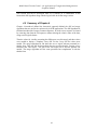
File 1
file 2
file 3
file 4
file 5
1.1
1.2
1.1
1.3
1.1
1.2
1.4
1.1
1.2* - - 1.3* - - 1.5* - - 1.2* - - 1.1
1.3
1.6
1.3
1.4
1.4
1.5
Å Look here
3.1.4 Branching and Merging
CVS allows the user to isolate changes onto a separate line of development, known as a
branch. When files on a branch are modified, those changes do not appear on the main
trunk or other branches. Later on, the user can move changes from one branch to
another branch or to the main trunk by merging.
An example of using branches would be when a release (say 1.0) later on proves to
involve a fatal bug. Instead of making a bug fix based on the newest sources (1.1), the
software designer instead creates a branch on the revision trees for all the files that
make up revision (1.0); thereafter modifications can be made to the branch without
disturbing the main trunk. When the modifications are finished the programmer can
elect to either incorporate them onto the main trunk, or leave them on the branch. It is
important to note that branches get created in the repository and not in the working
copy.
• Adding, Removing and Renaming Files and Directories
To add new files the user must have a working copy of the directory, and then create the
new file inside this working copy of the directory. The command ‘CVS add filename’
is used to inform CVS to perform a version control on the file. To actually check the file
into the repository so that other users can see the file, use the ‘CVS commit filename’
command. To add a new directory, use the add command.
To remove files, but still be able to retrieve exact copies of old releases, one must first
remove the file from the working copy of the directory. The next step is to use the ‘CVS
remove filename’ command. Finally use the ‘CVS commit filename’ to actually
perform the removal of the file from the repository. To remove a directory, first all files
in that must be removed in a similar fashion as described previously. The directory itself
can not be removed as there exists no way of doing that. Instead specify the ‘-P’ option
to CVS update which will cause CVS to remove empty directories from working
directories. Doing so will leave the users with the ability of retrieving old releases in
which the directory existed.
12
Model Based Version Control – An Application of Configuration Management on
Graphical Models
A simple and safe method of moving files is to copy old to new, and then issue the
normal CVS commands to remove old from the repository, and add new to it.
$
$
$
$
mv old new
CVS remove old
CVS add new
CVS commit –m “Rename old to new” old new
3.1.5 Multiple Developers
CVS supports concurrent development which implies that more than one developer can
work concurrently or simultaneously on the same project. The default model in CVS is
an unreserved checkout: the developers can edit their own working copy of a file
simultaneously. The first person that commits the edited version will do so without any
problems. The persons that commit after him or her will receive an error message, they
will have to merge their work with the checked in version of the first person. This is
usually performed automatically with no problems using the update command. The
modifications to a file are never lost when using the update command. If any changes
between two files are made too close, CVS will notify the user that an overlap has
occurred, and the file will include both versions of the lines that overlap, delimited by
special markers.
3.2 Rational Clear Case
The following is a summary of the user manual of Clear Case [CLEARCASE]. Clear
Case is another commonly used SCM tool, but is easier to use than CVS, mainly due to
its friendlier graphic user interface (GUI).
Rational Clear Case is a configuration management (CM) system that manages multiple
variants of evolving software systems. Clear Case maintains the complete version
history of the software development artifacts, including code, requirements, models,
scripts, test assets, and directory structures. It performs audited system builds and offers
multiple developer workspaces.
A major difference between Clear Case and CVS is that the former uses a graphical user
interface (GUI); the user picks and clicks with the mouse to perform the operations
required. The latter uses a command-line interface (CLI); the user issues the commands
by typing them into CVS using its language syntax. This implies that the CVS user must
be used to the syntax and nomenclature of the language, while on the other hand, the
Clear Case user can more easily click his or her way into the menus and commands.
Clear Case also uses a graphical representation of what changes have been made, and
who has checked out which files.
3.2.1 ClearCase Views
Files and directories are called elements, and the data repositories containing the
elements are called VOBs (Versioned Object Bases).
Accessing files is achieved by setting up a view, which shows a directory tree of specific
versions of source files. Clear Case includes two kinds of views: Snapshot views, which
copy files from data repositories (VOBs), and Dynamic views, which uses the Clear
13
Model Based Version Control – An Application of Configuration Management on
Graphical Models
Case multi-version file system (MVFS) to provide immediate, transparent access to the
data in the VOBs using a directory tree.
The snapshot view is best used when the computer does not support dynamic views, and
the user wants to work with source files support when disconnected from the network
hosting the VOBs.
The dynamic view should be used when the user wants to access elements in VOBs
without copying them into the computer, and when it is important that the view reflects
changes made by team other members at all times without having to update the data.
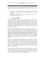
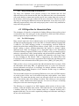
3.2.2 Versions, Elements and VOBs
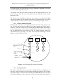
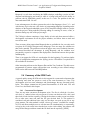
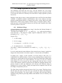
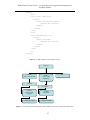
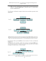
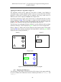
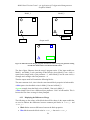
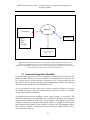
Each time a file or directory is revised and checked in, Clear Case creates a new version
of it. The files and directories are called elements and are stored in the VOBs. Figure 1
illustrates a VOB that contains the file elements prog.c, util.h and lib.c. Depending on
the size and complexity of the software development environment, Clear Case elements
may be distributed across more than one VOB. For example elements used by the
documentation group are stored in one VOB, while elements contributing to software
builds are stored in a different VOB.
Prog.c
0
Version 1 of prog.c used
to build release 1.2 of the
product
R
RLS_1.2
Util.h
Lib.c
0
0
1
1
2
2
Version 2
2
Version 3 used to build
release 1.3 of the
product
3
RLS_1.3
LATEST version,
being developed for
release 1.4
Figure 1: A VOB contains all versions of an element
3.2.3 Checking Out Files
Files that are under Clear Case control must be checked before any modification can
take place. That is achieved by first navigating to the directory where the file is located,
then right-clicking on the file and then choosing the Check Out selection. This opens
the check out dialog box, where comments can be provided describing what changes are
14
Model Based Version Control – An Application of Configuration Management on
Graphical Models
planned for the checked out file. Another option is to choose whether a reserved or
unreserved checkout shall be performed. Both reserved and unreserved checkouts are
supported. The reserved checkout has the exclusive right to check in a new version for a
given development project. In the unreserved checkout, the first view to check in the
element creates the successor; other developers working in other views must merge the
checked in changes into their own work before they can check in.
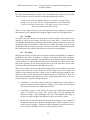
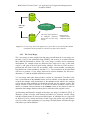
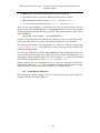
3.2.4 Checking In Files
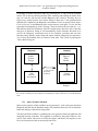
Checking in a file or directory element creates a new version in the VOB, which
becomes a permanent part of the element’s history, thus the element should be checked
in only when the user wants a record of its state.
If the checked in version is not the latest version in the VOB, the program will require
the user to merge the changes in the latest version into the version checked out in the
view. ClearCase will attempt to merge automatically by starting the Diff Merge tool.
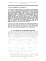
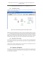
Prog.c
0
The version that the
user checked out
1
2
3
4
Users’ modifications to
checked out version
To create a new version the user
must merge version 3 into the
version that was checked out, and
check in the merge result, which is
version 4
Figure 1: Version 2 of prog.c was checked out and edited. Before checking it back in, someone else
checked-in version 3 of prog.c. When the user wants to check-in the new version, Clear Case informs that
it has to be merged with version 3 before becoming version 4.
15
Model Based Version Control – An Application of Configuration Management on
Graphical Models
3.3 Rhapsody and the Telelogic Family
Rhapsody is a visual programming development (VPE) tool developed by Telelogic for
real-time embedded software developers, and works by implementing solutions built in
UML 2.0 design diagrams that generate C++ code. To summarize, Rhapsody allows the
user to accomplish the following general tasks:
-Analysis: to define the system requirements in the UML language using a MDD
approach
-Design: perform edits and changes on the model
-Implementation: automatically generate code from the analysis model
-Testing: debug the model/code
Rhapsody uses the MDD architecture to allow the users, whether system or software
engineers, to achieve productivity gains over traditional document driven approaches.
This is achieved by allowing the user to simultaneously specify the system design
graphically (in the UML language) and to simulate and automatically validate it, while
it is being built. All of this will lead to the production of the code form the model of the
embedded system. [ILOGIX]
The Rhapsody software contains sample projects such as cars, an elevator, a CD player,
a dish washer, a ping pong game, Tetris and many other examples. A couple of these
projects were studied in order to try to understand the program more specifically. More
information is available in the tutorial section, and specifically the Rhapsody Tutorial in
C++.
3.3.1 Short about UML 2.0
To understand Rhapsody well one must have a thorough understanding of the UML 2.0
language. A short introduction to the UML language will be given here, but for more
detailed specifications please refer to [UML], [WIKI].
The Unified Modelling Language (UML) is an open source language for object
modelling using graphical blocks that are related to each other with the help of different
relationships. There are 13 different types of diagrams divided into 2 main categories
with one subdirectory, and they are:
1- Structure diagrams define what things must be in the model:
Class, component, composite structure, deployment, object and package diagrams
2- Behaviour diagrams emphasize what must happen/occur in the model:
Use case, activity and state machine diagrams
3- Interaction diagrams are a subset of behaviour diagrams that emphasizes the flow of
control and data among the things in the model:
Sequence, timing, communication and overview diagrams
16
Model Based Version Control – An Application of Configuration Management on
Graphical Models
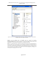
3.3.2 The Rhapsody GUI
The Rhapsody GUI is made up of three key windows and different toolbars for each of
the UML diagram types. The 3 main windows are: browser window, drawing area and
output window, while the 2 main toolbar windows are the modelling toolbar and the
standard toolbar functions.
1-The browser window: contains the directories and sub-directories of the entire model
in an expandable tree-structure
2- Drawing area: a sketching area where all UML models can be drawn
3- Output window: window at the bottom which displays messages
4- Modelling toolbar: contains the different tools necessary for drawing each UML
model
5- Standard toolbar contains common utilities such as windows toolbar, layout toolbar,
zoom toolbar and format toolbar.
Whenever a type of UML diagram is chosen the modelling bar automatically changes to
display the connectors and relationships that are used in that specific diagram. For
example when creating the use case diagram, the modelling toolbar displays buttons to
create a new use case, new actor, create association, and create generalization, flow and
dependency. When creating a sequence diagram the modelling toolbar will change to
display activities that are relevant to it.
3.3.3 Rhapsody in C++
The Rhapsody tutorial on building a mobile handset will now be completed and studied
to get more experience and create a wider discussion regarding file based and model
based control. The tutorial will not be described in detail because it can be accessed
from the program’s help menu -> List of Books, but rather only the main functions will
be highlighted and covered below.
The following will be treated in this thesis: system boundary box, actors, use cases,
association lines, dependencies, generalizations and requirements, creating a structure
diagram, drawing block diagrams.
The type of UML diagrams supported by Rhapsody:
Use case, structure, object model, sequence, activity, state charts, collaboration,
component and deployment diagrams.
A new empty project was created and named Handset. The first thing to do is to create
what is called ‘Packages’ which basically are folders that allows the user to organize
models using subsystem modules consisting of objects, object types, functions,
variables and other logical modules. These subsystems or packages are created by the
user in the browser window by right clicking the Package file and choosing ‘Add New
Package’, and then renaming each package in accordance. Here the importance of
having a solid UML knowledge is seen; since one must know what packages should be
created. It is also important to have a good theoretical and practical understanding of the
system being modelled.
UCD – Use Case Diagrams: display the main features of the system in an easy to
understand fashion, and also display the actors outside the system. This is done by rightclicking on the Analysis Package and choosing to add a new UCD and naming it (in this
17
Model Based Version Control – An Application of Configuration Management on
Graphical Models
example it was named ‘Functional Overview’). Then a new Boundary Box is created
and named ‘Handset Protocol Stack’ along with two actors the ‘Network’ and ‘MMI’
that will interact with the system.
This UCD has four use cases, and they are: place a call, receive a call, supplementary
services (messaging, forwarding, conference etc) and provide status (network status,
signal strength etc). Thus a use case is created for each of the four use cases and named
in accordance to their function.
The next step is to associate each of the actors with the use cases. For example the MMI
actor places and receives calls, while the Network actor notifies the system of incoming
calls and provides status. Thus, an association represents a connection between objects
or users. Another feature that can be represented is the Generalization in use case
diagrams, which is the relationship between a general and a more specific element, with
the specific element inheriting the properties of the general one. Thus Supplementary
Services will be a specific type of placing a call.
Now a new UCD called ‘Place Call Overview’ will be drawn and will contain 3 new use
cases: Place Call, Data Call and Voice Call. The difference this time being that the
Place Call will not be created; instead it will be chosen from the browser window and
dragged into the new UCD.
The next step is to create and name Requirements to show how they trace to the use
cases. For example a requirement called Req 1.1 stating that: ‘The mobile shall be fully
registered before a place call sequence can begin’ is associated with the Place Call use
case. Now dependencies can be created between the respective requirements and use
cases, using the Dependency tool. First the requirements are dragged from the Browser
Window into the UCD. Now the dependencies are drawn from the individual
requirements to the use cases. For example a dependency is drawn from Req 1.1 to the
Place Call use case. Dependencies can also be drawn between the requirements.
Stereotype is a function that can relate requirements to each other or to other model
elements, by extending the semantics of the UML model by typing UML entities. Two
types of stereotypes included are Derive and Trace:
-Derive: a requirement is a consequence of another requirement.
-Trace: a requirement traces to an element that realizes it.
Notes:
-Each time a new requirement was added into a model, even if the requirement exists in
the Browser window, one had to manually change its options to display its name.
- Right clicking a component and choosing ‘Remove from Model’ will delete it totally,
and it must be created again. To remove components from the view choose instead
‘Remove from View’.
The first moment will be to create Structure Diagrams that define the components of a
system and the flow of information between the components in a black-box perspective.
Structure diagrams consist of the following parts:
Objects, blocks, composite classes, ports, files, links, flows and dependencies
18
Model Based Version Control – An Application of Configuration Management on
Graphical Models
Start by right-clicking on the Architecture package and add a new Structure Diagram
and name it ‘Block Diagram’. The toolbar changes also and displays the following
tools:
Composite class, object, block, create port, link, dependency and flow
In the handset model there will be three blocks and they are: Connection Management,
Mobility Management and Data Link. These are created with the Block tool. Next step is
to add Objects that are the components of a system that form a cohesive unit of data and
behaviour.
Ports are another important feature in Rhapsody and they represent interaction points
between any class, object or block with its surrounding environment. They are
represented as small squares on the boundary of the class, object or block. The ports
have another distinctive feature; they allow the user to understand the architecture of the
system by specifying the interfaces between the system components and the
relationships between the sub-systems. Data Flows specify the information exchange
between the system elements at an early stage before committing to any specific design.
The data flow can be created between the ports of the objects and the blocks, and also
between the elements themselves. The direction of the data can also be chosen to be bidirectional form the features options.
For more information regarding Rhapsody please refer to the manual located in the help
menu. The following are the remaining types of diagrams that are supported in
Rhapsody but not covered in this chapter:
Structure diagrams—Show the system structure and identify the organizational pieces
of the system.
Object model diagrams—Show the structure of the system in terms of classes, objects,
and blocks, and the relationships between these structural elements.
Sequence diagrams—Show sequences of steps and messages passed between structural
elements when executing a particular instance of a use case.
Activity diagrams—Specify the overall control flow for classifiers (classes, actors, use
cases), objects, blocks, and operations.
Statecharts—Show the behaviour of a particular classifier (class, actor, use case),
object, or block over its entire life cycle.
Collaboration diagrams—Provide the same information as sequence diagrams,
emphasizing structure rather than time.
Component diagrams—Describe the organization of the software units and the
dependencies among units.
Deployment diagrams—Show the nodes in the final system architecture and the
connections between them.
3.3.4 More Telelogic Programs
The following section describes other interesting programs of the Rhapsody family:
SYNERGY Active CM
There has been some difficulties in attaining data regarding the following tools, and to
compensate for this many power-point presentations and video presentations were
19
Model Based Version Control – An Application of Configuration Management on
Graphical Models
attended to try and get as much data as possible regarding the usage and functionality of
the software.
To perform simple configuration management, the Active CM tool can be applied. This
tool integrates with the Windows Explorer by adding an Active CM tool bar along with
a to-do list when the documents are managed in SYNERGY. When a user wants to
perform a task, the system automatically updates the file version number by one, and it
allows the user to add a note on what was performed. The performed task is then
removed from the to-do list.
In the video example that was demonstrated in [VIDEO], a user opens the to-do list and
finds two different tasks. The first was “To add a company logo to a specification”,
where the document had the version number 4. He then adds a logo to the file and saves
it. The software automatically updates the CM Synergy repository to version 5 and he
adds a tag stating “Added company logo”. The to-do list is then re-opened and now
contains only 1 to-do action.
This is basic SCM and is developed for all users that do not have any previous
experience in using other SCM tools. Clearly the software does not handle more
complex functions and was not intended for software engineers, but rather for everyday
configuration tasks.
DOORS
This is a management tool that allows control and configuration management of any
project, by connecting the entire project team members, and allowing them to share
resources. In the demo [PRES] a team encompassing a product manager, project
manager, requirement analyst, software and test engineers, quality assurance and the
end user all interact using the tools available in DOORS/ERS (Enterprise Requirement
Suite). This software allows linking and tracing of documents across platforms and
users, so that for example a software engineer can link the coding statements to the
original requirement given from the sales department. The system allows also for
tracking document history. It also allows customers to connect to the database and ask
question or monitor the project progress, and allows electronic signing of documents.
Rhapsody Gateway (RG)
The RG is an add-on that allows traceability between different software to be shown in
Rhapsody. RG consists of configuration editors, converters and filters that take in a
large number of different files, such as Doors, Word, Excel etc and links between them
and produces an image of requirements traceability in relation to the project to be shown
in the Rhapsody interface [GATE]. This tool is studied further in chapter 7.
TAU
The TAU software is a tool that is similar to Rhapsody but with the difference lying in
its support for Model Driven Architecture (MDA) in comparison with MDD as well as
offering support for UML 2.0, UML testing, model simulation and code generation.
3.3.5 Conclusions Regarding Rhapsody
After having interacted with Rhapsody and studied its capabilities the following can be
said:
20
Model Based Version Control – An Application of Configuration Management on
Graphical Models
Rhapsody is a tool when considering the MDD technique: modelling a project in UML
diagrams and debugging and testing it while it is being built and have the ability to
generate code for embedded systems, in this case C++ code. The problem is that one
must understand UML 2.0 well.
It was advantageous to be able to generate the code in four languages (Java, C, C++ and
Ada) because it gives the user a free choice of programming language, depending on the
character of the targeted embedded system. It also simplifies changes made to a project
while the project is being modelled, allowing adding or removing of: actors, events, or
functions during any time of the project stages.
The Telelogic software constitutes a large family of tools and when mastered offers a
development environment for all the project members, and allows them to track and
trace all the work.
There are many white papers about Rhapsody that are available for free; one only needs
to register for a Telelogic Passport on the homepage. There are many free webinars too
that can be attended. The problem was that the papers were not of technical character,
but instead described the advantages in using Rhapsody, and the webinars were
presented by respective companies that displayed the interaction between their product
and Rhapsody.
There is no support for SCM as it was thought of in the beginning. To perform simpler
types of configuration management the Synergy Active CM add-on is required but is
not available for download.
Other interesting add-ons are the Reporter Plus and the Test Conductor. The add-ons are
programmed to generate reports and perform tests according to user defined settings
which can be done across the DOORS platform.
3.4 Summary of the SCM Tools
A general quality among all SCM tools is their support for concurrent development: that
is allowing more than one person to work on the same document at a time. This
development style has some advantages and disadvantages that are discussed briefly
below. This chapter summarizes the general functionalities of SCM tools CVS and
Clear Case, described in this chapter.
3.4.1 Concurrent Development
There are two main concurrent development styles. The first is called the “checkoutedit-check in” method, where only one person at a time can checkout a file, edit it and
then check it back into the repository. During the checkout no other person can edit the
file as other users must wait until the file gets checked back in. This method is
considered safe and traditional since only one developer can work on any file at any
given moment. The other method is called “edit-merge-commit” (available for example
in CVS) and allows multiple users to edit the same file simultaneously or concurrently,
as long as they work on the latest checked out version. After editing, the software will
merge all the changes and then commit the file back into the repository. [SINK]
21
Model Based Version Control – An Application of Configuration Management on
Graphical Models
Eric Sink, Software developer at Source Gear, and builder of the original version of the
“Internet Explorer” browser describes concurrent engineering as follows:
“Think of your team as a multithreaded piece of software, each developer
running in its own thread. The key to high performance in a multithreaded
system is to maximize concurrency. Our goal is to never have a thread
which is blocked on some other thread.”
Thus to keep a high efficiency in the development process, support for concurrent
development is vital, whether the development regards textual files or graphical ones.
3.4.2 The Diff
In text files, the Diff function will open up the current working version and the latest
checked in version as two separate windows next to each other. A certain color code
will highlight the differences, indicating what has been deleted, what has been moved to
other parts of the file and what new lines have been added. This makes it easier to spot
the differences between any two versions. There are many different algorithms and tools
for the difference tool, which will be discussed in the next coming chapters.
3.4.3 The Merge
Merging two text files is a basic part of everyday concurrent development as it enhances
productivity and allows developers to improve and update their work constantly.
Otherwise developers would have to spend endless time waiting for others to finish their
work and check it in. The problem of conflict arises when the users check in their work
back to the repository, due to the fact that the files were of the same base version when
checked out, but were checked in with different versions.
When user A checks in his work, the software updates the version number by one with
respect to the check out version. When user B now checks in his work, which was
checked out according to the same version as user A initially had, there might be some
conflict. In this case the software will complain that there are differences. There are
three common solutions to the problem: (1) is to attempt using auto merge; (2) to use a
visual merge tool; (3) perform changes by hand.
•
Auto Merge: is most often effective and rarely complains, but it may refuse to
produce a merged version if both users’ changes are in conflict with each other.
That occurs when both users modify the same line.
•
Visual Merge: using a visual merge tool can be of great help when auto merge
refuses to perform any merge. The visual merge tool will highlight the
differences using a certain predefined color code. This simplifies the merge as
the user can easily recognize the differences, and overcome the conflict.
•
Rewrite the File: the third option can be used when changes are too complex to
be made by hand, the user can restart editing the base version completely. This is
useful when, for example, a function has been completely removed from a user’s
version, and it would thus be easier to rewrite the entire version.
22
Model Based Version Control – An Application of Configuration Management on
Graphical Models
Examples of software tools that can be used for visual merge are Guiffy and Araxis
Merge. [ARA], [GUI]
3.4.4 Locking-Unlocking the Model
Most engineering tools allow the users to work concurrently on the same files, so that
work can be merged in some way when committed back into the repository. There is a
method known as locking and unlocking a model. In this way only one user can check
out a file and edit it, while all other users must wait until the file is checked back and
unlocked. The advantage of doing so is that it is guaranteed that only one person can
perform a change at a time, and no conflicts can occur when checking back the files into
the repository, but on the other hand there are the following serious disadvantages with
locking and unlocking models or files [TOR]:
•
Locking may cause administrative problems: A user that has checked out a file
may happen to forget about it, and leave it locked for a long time. This forces
other users to wait until they can perform their changes, thus loosing valuable
time. If the user that has locked the file is not present for a longer time due to
sickness or vacation, the other users must get an administrator to release the
lock. This only causes unnecessary delays, wasted energy and frustration for the
other users.
•
Locking may cause unnecessary serialization: If a user wants to edit the
beginning of a file, while another wants to edit the end of the same file, he or she
must still wait until the file has been returned and unlocked. This is also a
problem involving great waste of time. In this specific case, both users might
have worked concurrently on the same file without causing any loss to each
others work.
•
Locking may cause a false sense of security: Suppose that a user locks and edits
file A, while another user locks and edits file B, and that both file A and B are
dependent upon each other. In this case the changes that were made to the files
may cause them to become incompatible with each other. In this case the locking
system failed completely to prevent the problem of overwriting, and created a
false sense of security for both users. In this case the individual users thought
that by locking the file it would be safe to edit it, without causing
incompatibility to any other files. This problem would be solved by both users
discussing and solving the problem together, forcing them to find suitable
common time to discuss and solve the issue.
Another major problem would be if the users are located in different geographic
regions, making all of the three above disadvantages even harder to cope with. This
would add costs to the communication process such as national or international
telephones calls and regular meetings.
This chapter also described and discussed Clear Case and CVS, two major tools used in
SCM and the third tool: Rhapsody, used for MDD. The SCM tools functionality was
described and their major strengths explained, as well as how they primarily function.
The major functions presented are: the support for concurrent development, diff and
merge functions and locking and unlocking of models. Rhapsody on the other hand
supports MDD of UML models in order to produce code for embedded systems.
23
Model Based Version Control – An Application of Configuration Management on
Graphical Models
The following is a summary of the pros and cons of CVS and Clear Case.
CVS:
Pros:
-
Saves disk storage space: CVS stores only the differences between the versions
and uses these deltas to build the previous version
-
Supports concurrent development: advantageous when multiple users work on
the same project
-
Has few functions: relatively easy to learn
-
It is freeware
Cons:
-
CVS is not a system for writing the data files, only for keeping track of the
concurrent development
-
Difficult to view the deltas and understand the previous versions by just viewing
the deltas, thus the program must construct the version from the deltas
-
Not a substitute for developer communication: when a developer comes across a
conflict which is too difficult to solve on his own, he will have to solve it by
communicating with other developers
-
CVS does not have change control: the program does not keep track of all the
bugs and status of each of them
-
Used only for source file and does not support other document types
Clear Case
Pros:
-
Uses a graphical interface: simple to view and understand
-
Offers a view of the actual file history in a tree structure
-
Works for a wide variety of document types: word, excel, PDF
Cons:
-
Complex and has many built-in features that requires more time to learn
-
Stores the entire file and uses large amount of memory
-
When installed Clear Case integrates into the window explorer bar
-
Expensive software that mist be bought and licensed
24
Model Based Version Control – An Application of Configuration Management on
Graphical Models
4 The Analysis of Existing Algorithms: Flat vs.
Hierarchic
In this chapter, the difference and merge algorithms will be studied and analyzed since
these functionalities will be developed later on to be applied onto the graphical models
used in Simulink. There are two main different data models that exist: (1): simple, plain
or flat text files and (2): fine grained or hierarchically structured data. At first the
difference between these two types may not seem important as both types consist of
printed lines. The main difference lies in how the semantic of the data is defined and
how the algorithms are built when treating the data. Examples of simple, flat or nonstructured data are printed text documents and source code. Hierarchically structured
data on the other hand is XML and UML data in which the structure of the data is
semantic. Simulink models which will be presented later in this document are examples
of the latter type of data.
The first part of this chapter will cover the plain textual difference algorithm and the
second part will cover the plain textual merge algorithm. The two last chapters will
cover the fine grained or hierarchical data in which the details of the syntactical
structure of the document are considered.
It is important to state that this chapter describes the purely mathematical approach of
the algorithms. Thus it gives a deeper understanding of how the algorithms work on a
detailed technical level.
4.1 Diff Algorithm for Flat Data
The main idea behind the difference, or diff as it sometimes is referred to, is to feed two
revisions or versions of a textual file such as program code or any other text document
and output the differences between these documents in a neat fashion using a color code
in one single document. Thus the process of identifying the differences between two
objects involves two main steps: firstly identifying the differences in an efficient way,
and secondly displaying the differences correctly in a useful way, most often using
colors. This means that the parts or differences coming from revision one (v1) are
colored in a certain color, and the differences coming from the other revision (v2)
relative to the first are colored in another different one. Different colors are used
because it becomes easier for the user to view the differences than indicating it by
adding more text.
The main function of the program was to solve the LCS or Longest Common
Subsequence problem to find the lines that do not change between files in plain or linear
text files. At that time the output was shown textually using angle brackets (< and >) for
presenting line deletions and line insertions.
Today applications for diff algorithms include comparison of amino acid sequences in
the DNA research filed (and the answer to the question of 'how far apart are we?'),
storage reduction in a version control system, historical analysis of different copies of
old texts, and by the "patch" command to update source files without needing to replace
25
Model Based Version Control – An Application of Configuration Management on
Graphical Models
the whole file, using advanced and fast algorithms that operate in linear time and space
complexity.
4.1.1 Longest Common Subsequence
By definition a subsequence of some sequence is a new sequence which is formed from
the original sequence by deleting some of the elements without disturbing the relative
positions of the remaining elements. Take the following example:
< B,C,D,B > is a subsequence of < A,C,B,D,E,G,C,E,D,B,G >, with corresponding
index sequence <3,7,9,10>.
Now given two sequences X and Y, a sequence G is said to be a common subsequence of
X and Y, if G is a subsequence of both X and Y. For example, if
X = < A,C,B,D,E,G,C,E,D,B,G > and Y = < B,E,G,C,F,E,U,B,K > then a common
subsequence of X and Y could be G = < B,E,E >. This would not be the longest common
subsequence (LCS), since G only has length 3, and the common subsequence < B,E,E,B
> has length 4. The longest common subsequence of X and Y is < B,E,G,C,E,B >
Back to the original problem of finding the LCS or longest common subsequence
involves the application of computer algorithms, and there are many topics available on
that such as [BER], [LIB].
A straightforward method to compute the LCS(X,Y) consists in considering all the
subsequences of X, checking if they are subsequences of Y and keeping the longest of
them. [CHA]. One method, which uses a dynamic programming strategy, is the
polynomial time edition of the LCS which can be summarized in the following four
steps [ANSWERS]:
•
Analyze the LCS properties
There exist a large number of research topics on the LCS properties such as [GOE] and
[MAS]. One popular such is the LCS having an optimal-substructure property.
The Optimal-Substructure of an LCS Theorem is:
Let X = < x1,...,xm > and Y = < y1,...,yn > be sequences, and let Z = < z1,...,zk > be any
LCS of X and Y.
1. If xm = yn, then zk = xm = yn and Zk-1 is an LCS of Xm-1 and Yn-1.
2. If xm ≠ yn, then zk ≠ xm, implies that Z is an LCS of Xm-1 and Y.
3. If xm ≠ yn, then zk ≠ yn implies that Z is an LCS of X and Yn-1.
•
Devise a recursive solution compute the LCS
The second step involves finding a recursive solution to compute the LCS. There is a
common standard recursive formula for the LCS which has been agreed upon among a
vast number of computer scientists which relies on the Optimal Substructure Theorem
above, and is defined as the following:
26
Model Based Version Control – An Application of Configuration Management on
Graphical Models
For two sequences Xi and Yj of lengths m and n respectively, c[i,j] is the length of the
longest common subsequence in the sequences. The first part of the formula says if
either one of the sequences has length 0, then there can be no proper subsequence of a
null sequence. The other two parts breaks the LCS apart into smaller sub problems until
we reach the null sequence in a recursive fashion. [ANS]
•
Compute the LCS, using for example the Generic LCS Delta method
Computing the LCS can be done with many existing methods such as [HIR], [EPP], and
one common is using the Generic LCS Delta method which is in polynomial time.
LCS Delta algorithm takes the two sequences X and Y as inputs and creates a table c
with the lengths of X and Y. The algorithm also has a table b, which is a copy of c,
which is used to store the optimal solution of the LCS. The rest of the algorithm uses
the formula defined above to compute the LCS, and populate the table. The algorithm
runs in O(mn) time, where m and n are the length of X and Y respectively. There are
more efficient algorithms, namely LCS Alpha and LCS Beta, but this algorithm, the
LCS Delta is the most intuitive.
LCS-Delta(X,Y)
m <- LENGTH[X];
n <- LENGTH[Y];
for i <- 1 to m, do c[i,0] <-0;
for j <- 0 to n, do c[0,j] <-0;
b <- c;
for i <- 1 to m, do {
for j <- 1 to n do {
if (xi = yj) {
c[i,j] <- c[i-1,j-1]+1;
b[i,j] <- "UP-LEFT";
}
else if (c[i-1,j] >= c[i,j-1]) {
c[i,j] <- c[i-1,j];
b[i,j] <- "UP";
}
else
c[i,j] <- c[i,j-1];
b[i,j] <- "LEFT";
}
}
return c and b
The entire LCS algorithm given above runs in O(mn) in time and space.
•
Construct the LCS
The fourth and final step involves construction of the LCS. This is achieved by the
result of the above step which returns the table b (below) and is used to construct the
LCS. The b table could look something like this:
27
Model Based Version Control – An Application of Configuration Management on
Graphical Models
In this case the table initiates from the (m,n) position and continues following the
directions until it reaches the end of the LCS denoted by the ! mark. This computation
method is O(m+n) in time and space complexity. [CHA]
4.1.2 Representing the Differences
For plain textual difference approach two documents are fed into the algorithm. These
are called the base documents and it is between those that the differences should be
displayed. The document that will contain both the common and the specific parts of
both the base documents will be known as the unified document. This nomenclature
applies to both the simple and hierarchical data models.
In the plain textual approach both base documents are placed next to each other and the
common parts are arranged in a side-by-side fashion in two adjacent columns. The
differences are highlighted to indicate which changes lay within each base document
relative the other.
Thus for example one color is defined for each version of the document and a third
color is chosen to indicate that there is a difference between the data. For example one
can allocate the green and blue color respectively to each of the two documents and red
to indicate existence of a difference between them.
4.1.3 2-way vs. 3-way Difference: Presenting the Differences
It is apparent that the common parts in both base documents should be represented only
once in the unified document. Thus the final unified document will consist of both the
common parts and the specific parts of each base document. Different colors are used
for displaying the differences. An interesting aspect discussed in [OHST] is the
following: If the colors are removed from the unified document, does it result in a type
of “merged” document? This is false since a merged document is associated with
removing conflicts in a logical method. In that sense the unified document is not a
merged document. This topic will be covered in the chapter of the merge algorithm.
This thesis will cover the 2-way diff which as its name indicates finds the difference
between two base documents. There is another type of diff known as the 3-way diff in
which three base documents are implemented. In this latter method two documents are
direct children versions of the third, thus the three base documents lie in parallel
branches of a version tree.
The way to present differences is by using different colors to show which changes came
from which respective revision or base document. For the 2-way difference an optimal
number of colors are three: one color for each revision such as green and blue, and one
for the different parameters (usually red).
For the 3-way difference five different colors are needed: one for the common parts,
also a standard such as black, two colors for presenting insertions and deletions in the
first branch and two for changes in the second branch. This may become rather too
colorful and becomes a debated issue if the user can maintain an overview of the bulk of
information presented in the unified document.
28
Model Based Version Control – An Application of Configuration Management on
Graphical Models
4.2 Merge Algorithm for Flat Data
This subchapter will define the term merge, and also introduce the 3-way merge
function, in which three documents are needed to complete a merge. Again the word flat
is used since the data has no hierarchy and a document is simply regarded as printed
lines of text.
Merging is used today in many everyday applications such as in PDAs (Personal Digital
Assistant) or handheld computer synchronization. This occurs whenever the user
performs synchronization between a computer and a PDA; a memo added on the PDA
should also be visible on the computer. Another usage is in computer patches, where a
patch represents a textual difference between two text files, and is merged with an older
version to produce a newer one.
4.2.1 Definition of Merge
A formal definition of the technical term “merge” taken from the National Institute of
Standards and Technology [NIST] is:
“The input is two sequences, A={a1, ..., an} and B={b1, ..., bm}, each sorted according to
some total order, ≤. The output is a single sequence, merge(A,B), which is a sorted
permutation of {a1, ..., an, b1, ..., bm}.
merge(A, B) is
1. A, if B is empty,
2. B, if A is empty,
3. {a1}.merge({a2, ..., an}, B) if a1 <= b1, and
4. {b1}.merge(A, {b2, ..., bm}) otherwise.
The symbol "." stands for concatenation, for example, {a1, ..., an}.{b1, ..., bm} = {a1, ...,
an, b1, ..., bm}.”
It is to be noted that this formal definition of the technical term of merge is applied for
integers since the total order is less than or equal i.e. it involves the use of numbers.
So simply put, a merge, or more precisely a two-way merge in this case, is a
combination of two different objects, such as vectors containing letters or digits that are
combined in a certain fashion to form one object which will contain both common parts
of the objects and some or all of their differences. It is then up to the user to decide
which changes are to be merged, the ones coming either from the first or second
version. This method is similar to and based on the difference algorithm defined in the
previous chapter to define the differences, and with the only difference being on
deciding how to resolve conflicts. Finally, the output will be composed of the file and
the changes incorporated by the user.
The figure below describes the general layout of the 2-way merge. This figure shows
that the input data must be of the same type, and that the output will include both
common and shared data. The merge engine is left empty and could host different
algorithms using different processing methods with different levels of efficiency and
complexity.
29
Model Based Version Control – An Application of Configuration Management on
Graphical Models
File 1
Merge Engine
Same type
of data
File 2
The merge engine depends on
an intelligent comparison
between the two files being
merged
Merged
File 1-2
Merged file has:
-Common content
-Additional content
Figure 2: A two-way merge. This can be applied to any types of files as long as the algorithm handles
reading them and the input data are of the same type that is flat or otherwise.
4.2.2 The 3-way Merge
The 3-way merge is more complex but also more powerful than the 2-way merge as it
provides a way to also synchronize data [DXML], and involves as its name indicates
three different documents to initiate. The 3-way merge is widely used in concurrent
development, for example when two different users check out a copy of the latest
version v, and want to check it back in after editing it. The first user will not face a
problem and will check in the file successfully, with a version number exceeding the
last checked out version number by one that is v+1. The second user on the other hand
will have to perform a 3-way merge, between his current document, the first users’
document (v+1) and the original checked out version v.
A 3-way merge takes place between three versions of a document. First there is the
user’s version known as the selected version, and it is with this version that one wants to
reconcile the changes with. Second there is the current version which is the working
version that has been modified, and should be merged into the selected version. The
current version is called so because it is the last or newest available version of the
model. A common reference known as the common version is also chosen in order to
determine what changes that have taken place in reference to the original version.
An interesting and illustrative example on the three way merge is available in [TIG]. It
illustrates a picture of a tiger with whiskers and white eyes (common version). Along
with this original picture are also two modified copies, in which the first is a tiger with
no whiskers (current version) and in the second a tiger with yellow eyes and whiskers
(selected version). After performing a 3-way merge, the final picture will show the tiger
with yellow eyes and no whiskers.
30
Model Based Version Control – An Application of Configuration Management on
Graphical Models
Derived
from
File 1
Merge Engine
Base File
File 2
Derived
from
The 3-way merge engine
depends on identifying the
edits made and combining
them intelligently
Merged
File 1-2
Merged file has:
-Common contents shared
-Edits from file 1
-Edits from file 2
-Conflicts resolved
Figure 3: The 3-way merge overview. This can be applied to any types of files as long as the algorithm
handles reading them.
Figure 3 above shows the general layout of the 3-way merge, and indicates that file 1
and 2 are derived from the base document. All three documents are fed into the merge
engine and results in the final merged result. Regarding the merge engine, one may use
different algorithms with different efficiencies and complexities.
Applying the 3-way merge may result in a total of 14 different cases presented below
covering all possible outcomes, where files may differ or not. For the case where all
three files exist
•
all 3 may be identical (1 case)
•
each of the 3 pairs may be identical (3 cases)
•
all 3 may differ (1 case),
thus resulting in a total number of five (5) different cases.
Now, for the three cases where only two files exist: either they differ or do not differ,
giving a total of six (6) cases. Along with the three (3) cases where one file exists in
only one version gives a total of 14 cases (5+6+3). [RCS]
Thus the following table can be regarded as an algorithm for the 3-way merge, where
any of the 14 cases can exist. It is made up of four columns representing the case
number and type, the action that will be taken by the program, and an explanation of
that specific action.
By implementing a program that starts be applying a difference between the files, one
can write a program that uses the results of the differences to go further on. Take the
following as an example: If a difference is run between the files with a zero result,
which means no change has been detected between the files; then the program will use
31
Model Based Version Control – An Application of Configuration Management on
Graphical Models
case 1 and prompt nothing. This is applied to cover all the five cases and construct a
useful 3-way merge tool.
First, the 5 cases where all three files exist:
Case No
Case
Action
Explanation
1
All files equal
No prompt
Since no changes have been
made to any of the data.
2
All files differ
Prompt merge
There are no equivalent files
among the three files in each
version. It is assumed that the
user is interested in merging
the selected version's changes
with the current version.
Therefore, the default action is
to merge.
3
Selected file
differs
Prompt replace
The version of the file is
unchanged from the common
version, yet the selected
version has been modified. It
is assumed then, that the
selected version of the file is
more up to date, and the
default action is to replace the
users file with the file from the
selected version.
4
Working file
differs
No prompt
The selected version has no
changes to incorporate
5
Common file
differs
No prompt
The working and selected
version have both changed, but
the changes are identical, so
there are no changes to
incorporate into the working
version.
Secondly, the 3 cases where only one pair of files exist but are equal:
Case No
Case
Action
Explanation
6
Common and
Selected.
Prompt nothing.
The user deleted a file and the
selected version didn't. The
selected version has not been
modified, so it is assumed that
the file is obsolete.
7
Common and
Working
Prompt delete.
The selected version deleted a
file that the user has not
32
Model Based Version Control – An Application of Configuration Management on
Graphical Models
modified, so it's assumed that
the file should be deleted.
8
Working and
Selected.
No action.
Both versions have added an
identical file, there are no
changes to incorporate
Thirdly, the 3 cases where only one pair of file exists but are different:
Case No
Case
Action
Explanation
9
Common and
Selected.
Prompt nothing.
The user deleted a file and the
selected version didn't. The
selected version has been
modified. This type of conflict
cannot be merged, the user
must decide what to do. The
default action assumes the
deletion is correct.
10
Common and
Working.
Prompt delete.
The selected version deleted a
file that the user has modified,
so it's assumed that the file
should be deleted, even though
he/she modified the file.
11
Working and
Selected.
Prompt merge.
Both versions added a file and
the files differ. The merge will
take place with an empty
common file, and is likely to
produce serious changes.
Finally, the 3 cases where only a single file exists:
Case No
Case
Action
Explanation
12
Common.
No action.
Both versions deleted the file,
so there are no changes to
incorporate.
13
Working.
No action.
Working version added a file;
selected version has no change
to incorporate.
14
Selected.
Prompt add.
The file exists only in the
selected version and is
assumed to have been added.
33
Model Based Version Control – An Application of Configuration Management on
Graphical Models
4.2.3 Merge: Relationship to the Difference
The merge was explained in the previous section as the function that will find
differences between two documents and ‘bake’ the differences into a new document that
will contain both the common parts and the specific ones coming from each revision of
the document, while leaving any conflicts for the user to decide on. Thus the first stage
of a merge is detecting the differences between the documents, if any such exist. So if a
difference program already exists, and works properly, then it can be easily modified for
usage in the merge program.
4.3 Diff Algorithm for Hierarchical Data
This subchapter will describe an algorithm for finding differences between fine grained
or hierarchical data. The main types of data considered are XML and UML structures,
and the program developed in this thesis is of this type too.
4.3.1 The XML Language
Many research topics have been conducted on the use of the differencing and merging
on higher hierarchical languages such as the XML or eXtensible Markup Language that
it stands for. The XML language provides a non-proprietary universal format for
sharing hierarchical data among different software systems. XML is a verbose plaintext
format, making it robust, platform-independent and legible1 to humans without
additional tools. XML was designed to be a deployable subset of the Standardized
Generalized Markup Language (SGML), which is widely used by government agencies
and major corporations to ensure interoperability and persistent data accessibility. XML
is currently being heavily pushed by the industry and community as the lingua franca
for data exchange on the Internet. XML is supported by the World Wide Web
Consortium or W3C as well as major corporations such as Microsoft, Sun Microsystems
and IBM. For more information about XML please refer to [XML], [W3] and [LIN].
XML provides a way to mark up content that adds information about its purpose. With
the information stored using XML, an application known as a parser can extract the
relevant information and process it accordingly for multiple situations resulting in a
hierarchical data structure. Examples of the situations include usage in databases,
servers and in editors. [IBM]
The most suitable structure for representing XML data is trees, since all XML elements
are strictly nested. All the trees are described using three main qualities: roots, labels
and orders. This means that data has exactly one root node, all the roots are associated
with a value and the order of the siblings is essential. Thus referring to a tree now only
requires a rooted, labelled and ordered reference. For more on the topic of labelling
terms please refer to the interesting topic [KYR].
The following is an example of an XML fragment which consists of the tree node:
library which has children nodes: books. Each child node has a title attribute and
a content child node. Each of the content nodes has a chapter attribute and a
keyword child node. The tree can be expanded by adding new book nodes and filling in
the new relevant information.
34
Model Based Version Control – An Application of Configuration Management on
Graphical Models
<library>
<book>
<title> Intro to XML</title>
<content>
<chapter title=”An XML fragment”>
<keyword> XML </keyword>
</chapter>
</content>
</book>
<book>
<title> UML Modelling</title>
<content>
<chapter title=”UML”>
<keyword> UML </keyword>
</chapter>
</content>
</book>
etc...
</library>
Figure 4: An XML fragment of a book library system
<Library>
<Book>
<Title> Intro to XML
<Book>
<Title> UML
Modelling
Etc…
<Content>
<Content>
<Chapter>
title=An XML
fragment
<Chapter>
title=UML
<Keyword> XML
<Keyword> UML
Figure 5: A tree structure system depicting the XML fragment code shown in the previous figure above
35
Model Based Version Control – An Application of Configuration Management on
Graphical Models
4.3.2 The Theory of XML Document Versioning
This section introduces the theory behind documents versioning of XML and will
describe the edit scripts that are used for representing document changes.
The traditional document versioning systems are edit-based, edit scripts are used for
representing changes in documents, also known as deltas, and also for reconstructing the
versions incrementally. The edit scripts are introduced in more detail in section 4.3.4
Edit Scripts: Cost Models. There are two types of edit scripts: reverse editing and
forward editing scripts. The difference between these is that the reverse editing script,
like the one used in RCS, [TIC], stores the most current version of the document
entirely while previous versions are stored as reverse editing scripts. The scripts
describe how to go back from one version to another in the document’s development
history. These deltas or differences are used in building in what is known as a minimum
cost edit script. The minimum cost edit script for two trees is defined using node insert,
node delete, node update and sub-tree move as the basic editing operations.
The problem of finding what data is similar in two objects can be complex and time
consuming, but since Simulink models have identifiers they will simplify this task.
As an example, consider the two trees T1 and T2 shown in Figure 6 and Figure 7. The
number inside each node is the node’s identifier and the letter inside each node is its
label. All of the interior nodes have null values not shown here for simplicity. Leaf
nodes have the values indicated in parentheses. Thus these trees could represent two
structured documents where the labels D, P and S denote Document, Paragraph and
Sentence respectively. The values of the sentence nodes are the sentences themselves.
This is one of the advantages of XML: the trees can be used for representing an infinite
amount of systems as long as they are defined correctly for that specific system
[CHAW].
T1 represents the older or initial version while T2 represents the newer or later version.
When one wants to determine an appropriate transformation from T1 to T2, the primary
task is to find the two nodes in the two trees that remain unchanged. In our models these
two nodes are assumed to be the unchanged.
36
Model Based Version Control – An Application of Configuration Management on
Graphical Models
D: 1
P: 3
P: 2
5
S(a)
6
S(b)
7
S(c)
8
S(d)
P: 4
9
S(e)
10
S(f)
Figure 6: Tree T1 consisting of 3 paragraphs (P) and a total of 6 sentences (S)
D: 11
P: 12
15
S(a)
P: 14
P: 13
16
S(c)
17
S(f)
18
S(d)
19
S(e)
20
S(g)
Figure 7: Tree T2 also consisting of 3 paragraphs and 6 sentences
By looking carefully and comparing the two trees one understands their structure and
notices the following differences: the numbering of the nodes starts at the root and
continues incrementing as one move to the right throughout the tree (breadth first
labelling).
37
Model Based Version Control – An Application of Configuration Management on
Graphical Models
Moreover the following can be noticed: node 5 in T1 has the same value S(a) as node 15
in T2 thus nodes 5 and 15 should probably be the same. Similarly nodes 4 and 13 have
one child each with the same value S(f) and thus should probably correspond.
An interesting discussion is: how detailed should the match be? To simplify the
matching two terms are introduced: partial and total matching between the trees. Partial
matching is when some of the nodes in the two trees participate, while the matching is
total if all the nodes participate. Most often the matches are partial, but it depends of
course on the number and size of changes that have been made to a tree. It is thus less
likely that the matches are total matches, but one would like to match nodes that are
approximately equal. For instance node 3 in T1 should match node 14 in T2 even though
node 3 is missing the child S(g) .
The term isomorphic is introduced in [CHAW] to indicate that two trees are identical
except for the node identifiers. For trees T1 and T2 once a partial matching, M, is found
the next step would be to find a sequence of operations that would transform tree T1 into
another tree T´1 that is isomorphic to tree T2. The changes that are involved in the tree
T1’ may include deleting nodes, inserting nodes, updating the values of the nodes and
moving entire nodes along with their sub-trees. The next step would be take the partial
matching M and extend it into a total matching M´ between the trees T´1 and T2. This
new total matching M´ now defines the isomorphism between the trees T´1 and T2.
The sequence of change operations between the two trees is called edit script, and the
goal is to find one such that uses a minimum number of changes. To fulfill this goal
each edit change is given a cost, and now one must find a minimum cost edit script, also
referred to as the Minimum Conforming Edit Script (MCES).
4.3.3 Edit operations
This section will describe each of the edit operations that are used for transforming one
tree into another. In an ordered tree let the nodes v1… vm be children nodes of u, then
naturally vi is the i:th child of u. For a node x let l(x) denote the label, v(x) denote the
value and p(x) denote the parent of x, if x is not the root. Now T1 will refer to the tree on
which the operations are to be performed on and T2 refers to the resulting tree. The four
edit operations will then be:
•
Insert: The insertion of a new leaf node x into the tree T1 is denoted by
INS((x,l,v),y,k). This stands for a node x with label l and value v is inserted as
the k:th child of node y of T1 .
•
Delete: The deletion of a leaf node x into the tree T1 is denoted by DEL(x). This
operation will result in a tree T2 which is similar to tree T1 except that it does not
contain the node x. This operation does not change the relative ordering of the
remaining children of p(x).
•
Update: The update operation updates the value of a node in a tree x in T1
achieved by UPD(x,val). T2 is the same as T1 except that in T2 v(x) = val.
38
Model Based Version Control – An Application of Configuration Management on
Graphical Models
•
Move: The move operation moves an entire sub-tree from one parent node to
another in T1 denoted by MOV(x,y,k). T2 will be the same as T1 except for that x
becomes the k:th child of y.
The following is an illustrative example of how the insert and delete operations can be
implemented.
1
2
Tree T1
3
4
5
1
Tree T2
2
3
5
4
6
M(Hello)
Figure 8: Illustration of the insert operation. By applying the operation INS((6,M,Hello),3,2) to tree T1
(the upper one) results in the lower tree T2. This is explained by adding a node 6 with label M and value
´Hello´ as the second child of the third node of tree T1. The remaining labels and values are not shown.
By applying the delete operation DEL(6) on the second tree T2 above one obtains the
initial tree T1.
To illustrate the move operation, consider the second tree T2 and apply MOV(3,1,1).
This will result in a new tree T3 (below) by moving the third node and its entire children
to being the first child of node 1 as shown in figure
1
3
2
4
Tree T3
5
6 M(Hello)
Figure 9: The new tree T3 after applying a move MOV(3,1,1). That is moving the node 3 and all of its
children to the new location as first (1) child of node 1.
39
Model Based Version Control – An Application of Configuration Management on
Graphical Models
4.3.4 Edit Scripts: Cost Models
Now the four different edit operations have been introduced it is time to introduce the
edit scripts. By definition an edit script is a time ordered sequence of edit operations that
transform a tree T1 into a tree T2. A general method for representing an edit script is
using arrows (→) between two trees to indicate the application of an edit operation.
Thus, the edit operation e1 that is applied to a tree T1 to transform it into a tree T2 is
represented by: T1 → e1: T2. This representation is used for any number of edit
operations for the total transformation from the initial tree into the final tree.
There are many different ways to realize a tree from its initial tree model. For example
instead of applying a move operation on tree T1 or a sub-child of it, one can delete the
entire node (DEL) and its children, and then add them one by one (leaf by leaf) using
the insert operation (INS). This latter method is clearly more time consuming; so to
apply a measure of how time effective any given script is, the term cost of an edit
operation is introduced. The cost of an edit operation depends on the type of operation
and the nodes involved in the operation.
A general model is letting CD(x), CI(x) and CU(x) denote the cost of deleting, inserting
and updating a node x, and let CM(x) be the cost of moving a sub-tree with its root in
node x. The costs generally depend on the position of node x in the tree and on the label
and value of it. For simplicity the costs of deleting, inserting and moving a node x is
assumed to be unit cost, that is CD(x) = CI(x) = CM(x) = 1.
For the cost of updating, a new function is introduced: compare. This function inputs
two nodes as arguments and returns a value between zero and two [0,2]. The idea
behind the compare function is to decide whether the two inputs are close to each other
or different in value. So supposing that x is moved and its value v is updated to v´ close
to the initial value, then running the compare will result in a value less than 1 since the
cost of moving and updating x must be less than the cost of deleting and replacing it
with a new one with value v´. In a similar manner, if the inputs v and v´ are different
then it would be more cost efficient to implement an edit script containing a delete and
insert operation pair [CHAW].
The final cost result of the edit script is the sum of the cost of the individual operations.
This result is proportional to the number of changes and the size of the trees. Smaller
trees have lesser nodes and require a relatively smaller number of edit operations than
larger trees, taking a proportional number of changes.
4.4 Merge Algorithm for Hierarchical Data
The merge algorithm for hierarchic data relies on the ‘diff’ algorithm for hierarchical
data discussed in the sections above.
Thus, the same table introduced above in section 4.2.2 The 3-way Merge and involves
the first five cases. It consists of five possible outcomes: (1) all files are equal; (2) no
files are equal and three cases (3), (4), (5) where each case consists of one of the three
files differing from the other two.
40
Model Based Version Control – An Application of Configuration Management on
Graphical Models
This section will not be developed more as it consists of a combination of the
hierarchical diff algorithm along with the logical table in the flat merge section.
4.5 Summary of Chapter 4
Chapter 4 introduced defined the theoretical approach behind the diff and merge
algorithms that are used in the various tools in SCM applications. The diff algorithm for
flat data introduced the Longest Common Sequence, in which a new sequence is formed
by removing data from the old sequence without altering the relative order of the data,
using a strict logical scheme.
Then the colors for visually presenting the differences were discussed, and three colors
were needed to display a complete 2-way diff. For the 3-way diff five colors were
needed. The merge algorithm for flat data also uses a logical scheme presented in a
tabular form. Then the diff for hierarchical data was presented and it consists of tree
structures and ‘edit scripts’. The goal of the edit script was to find the optimal cost
models. The merge algorithm uses the same procedure but complements it with the
tabular form.
41
Model Based Version Control – An Application of Configuration Management on
Graphical Models
5 The Desired Tool Specifications
This chapter describes the desired algorithms of the programs for the Simulink models.
This is partly done using the API of MATLAB presented in the chapter above along
with the other useful functions that are developed here. It must be clear that the
algorithms of the textual algorithms can not be immediately implemented without
making certain assumptions or simplifications. This is mainly due to the difference in
structure of the two types of objects: text files and Simulink graphical models. For
example an assumption is made regarding the size of the files. In textual files,
documents containing literally thousands of lines, say 10’000 lines, are considered
extremely large and the complexity of the algorithm, whether linear or otherwise has an
important effect on the accuracy and time complexity. The graphical models employed
in this thesis are multi-levelled and contain multiple nodes; they are still relatively
smaller than the large text files. So no models containing thousands of blocks and
hundreds of levels were ever employed for the sake of simplicity.
It must be pointed out that this chapter describes the desired properties of the diff and
merge programs, but it does not mean that all the properties were developed
successfully. For more about what was developed please refer to the next chapter.
Secondly the complex diff and merge algorithms that were introduced and discussed in
chapter 4 are not implemented in the development of the desired specifications.
5.1 Considerations for the Model Based Approach
For version control of text based files, the CM software does not take the logic of the
file content into consideration. When performing a version control between two files,
the system only compares the files line by line and lists the differences using a certain
predefined color code. The different colors indicate the different changes such as what
lines have been moved, deleted or changed etc. depending on the software. Diagrams
can not be reasonably displayed in this manner, because one has to distinguish between
differences in the layout and differences in the conceptual diagram elements [OHST].
A graphical model has two important features of data, known as the layout data and the
model data. These two data are different with respect to their definition and content.
The layout data are defined as the positions and the sizes of the nodes in a diagram or
the position of corner points in edges; that is everything that would essentially be
considered as irrelevant in the textual representation of the diagrams content. The model
data on the other hand express the semantics of the document.
After having tested and edited models in Simulink the following can be concluded:
Blocks in models can be edited and changed in several ways. Parts of the model can be
created, deleted or shifted. The individual differences between two versions of one
diagram can be classified as intra-block differences and structural differences, by
dividing up all the object parameters into the following two differences:
•
Intra-block differences are differences within a certain block in the model.
Examples of such intra-block differences are parameters such as priority and tag.
Some of these properties are not directly visible in the model, since the block
properties editor must be opened before such differences can be seen.
42
Model Based Version Control – An Application of Configuration Management on
Graphical Models
•
Structural differences cover changes when blocks are shifted, created or
removed. Other structural differences are changes made to the size, position, and
color of the blocks. These changes are also defined as visual ones; they can be
seen immediately in the models.
Thus all changes in our models come from the object parameters of the blocks, but in
this case they have been divided into the two different categories just mentioned.
5.1.1 The Input and Output Types
The input files will consist of two Simulink models supplied by the user. The output
model will bear the name supplied by the user, and is composed of a Simulink model
that displays for the user the similarities and differences between the input models. The
goal of the output file is not to contain too many colours since it will confuse the user.
5.1.2 Colour Scheme
In the theory section of the thesis it was discussed that three (3) colours are optimal for
displaying the differences between two (2) versions. Black is the colour for displaying
no difference between blocks. According to the theory in this thesis two colours, one for
each model version should be used to indicate insertions and deletions such as blue and
green. A third color, red, will be used to indicate a property difference in a block.
5.1.3 Limitation
A limitation is that the upper most subsystem that contains the entire model cannot be
altered in any matter. This means no position changes, no property changes and no
addition nor deletion of blocks at that level. This is so because it will be used in naming
the models and the names of the models must remain unchanged to avoid confusion
when running the program.
5.2 Desired Use Case of the ‘Difference’ Program
The following is the use case of the ‘difference’ program and will define its working
process, the type of inputs, and the type of output that the program will generate.
•
It shall be based on modules meaning that it will be made of smaller programs
that work together to achieve the goal.
•
The goal of the ‘difference’ program is that the user will input two Simulink
models and the result is to show the differences between them graphically using
colours. The comparison will be performed by finding similar pair of blocks in
the two models, thereafter their block properties will be compared to find any
differences.
•
The differences between the two blocks will be displayed in two ways:
graphically using colours in a new model and in written form in the MATLAB
script window. If a block does not have a similar counterpart it will be shown in
a different colour implying that the block exists in only one model and not the
other.
43
Model Based Version Control – An Application of Configuration Management on
Graphical Models
•
The algorithm will be recursive, thus it will result in a compact and easy to
follow program code.
•
The result of the program will be a new graphical model that bears the output
name defined by the user and will include or display the common and different
blocks by using colours and texts to indicate those.
All of the above points of the use case are discussed in more detail in the next chapter.
5.3 Desired Use Case of the Merge Program
The following is the use case of the ‘merge’ program and will define its working
process, the type of inputs, and the type of output that the program will generate.
•
It shall be based on modules meaning that it will be made of smaller programs
that work together to achieve the goal and have a recursive algorithm.
•
The goal of the ‘merge’ program is that the user will input two Simulink models
and the result is to show one final model including common parts and the
differences chosen by the user. The comparison will be performed by finding
similar pair of blocks in the two models, thereafter their block properties will be
compared to find any differences.
•
When differences are discovered the user shall be informed by a message and
will decide on which version to implement. The differences between the blocks
will be displayed in two ways: visually using colours and in written form in the
MATLAB script window.
•
The algorithm will be recursive, thus it will result in a compact and easy to
follow program code.
•
The result of the program will be a new graphical model that bears the output
name defined by the user and will include or display the common blocks and the
ones chosen by the user.
All of the above points of the use case are discussed in more detail in the next chapter.
The goal of the merge program is to allow the user to input 2 graphical models and let
the program find the differences, to finally produce a third model containing the
common blocks, and allow the user to decide on which blocks to add when conflicts
arise. A main difference between this merge program and the ‘difference’ is that this
program will interact with the user when conflicts are discovered. This is done when a
change has been performed to the same variable in two different models. The user will
be prompted to choose from which model to incorporate the changes from.
5.4 Summary of Chapter 5
Chapter 5 described the specification of the desired programs that will be developed. It
described the different colour scheme that should be used in displaying the differences
between the models and also defined the desired use cases of both the diff and merge,
which is how the programs should work when completed. Thus the programs shall be
composed of modules and be recursive. For the actual programs that were developed
and how well they worked please refer to the next chapter.
44
Model Based Version Control – An Application of Configuration Management on
Graphical Models
6 Implementation of Model Based Tool
This chapter will describe the actual developed programs and describe what worked and
what did not relative to the use case. It will cover all of the use case specifications that
were defined in chapter 5.
6.1 The Input and Output Models
The program inputs are Simulink models, built of the basic and common types of
blocks. These can be either simple or multileveled models by using the subsystem
blocks. One important case is that whatever graphical model used it must always be
contained in a top-level subsystem block. This was chosen so that one can indicate if
any changes have been done inside the subsystem by colouring that subsystem.
The user will name the input by indicating the model name followed by the subsystem
name, separated by the slash character. Supposing that a model name is ‘wing’ and the
top-level subsystem name is ‘motor’ then the input name to the program would be
‘wing/motor’.
The output model will be made up of a new model, named after any desired name
allocated by the user. This name should be chosen so that it will indicate some
information about what two versions were compared.
Rerunning the programs with the same name of the output model as an existing open
one will not cause any problem. The program will close the previous output model
without saving it and open a new one with the same name.
6.2 Actual ‘Diff’ Program
The following sections will cover the actual difference program: a modularised and
recursive approach.
6.2.1 Modules
The main module was the ‘findDifference’ because it contained the algorithm that
checked for the differences and requested the displaying of the block in different
colours. The remaining modules were composed of small programs that performed
different tests to check if models exist or not. Here are the modules that were developed:
1- checkDifference(model1, model2, output): this program checks if the
output model exists and is open. If so it will close it without saving it and call
on startDifference. Otherwise it will directly call on startDifference.
2- startDifference(model1, model2, output): this module will create the
empty model with the requested output name. It then proceeds to call on two
main programs: findDifference and findDifference_Reverse.
3- findDifference(model1, model2, output): this is the main program
responsible for finding the differences between the models and displaying the
output in the output model. The main algorithm is located within this module. It
contains the following modules:
a. entity_directChildren (‘model’, 'block'): this module returns
all the direct child of ‘block’ type for ‘model’
45
Model Based Version Control – An Application of Configuration Management on
Graphical Models
b. block_uniqueIdentifier(‘block’): This module defines a unique
identifier for each ‘block’
c. entities_entityMatchingUniqueIdentifier(entitiesToCompare,
identifier) this module returns a matching unique block with a
defined ‘identifier’ by comparing it with the set of blocks in
‘entitiesToCompare’
d. block_differentProperties(block1,block2) returns the different
property between ‘block1’ and ‘block2’
4- findDifference_Reverse(model1, model2, output) is the second logic
part of the overall program that loops through the blocks in model2 and adds the
blocks that only exist in model2 as green.
6.2.2 ‘Difference’ Algorithm
The second part of the use case was to have two models as input and get one model as
output. The algorithm is described below:
The syntax for running the ‘difference’ program is:
checkDifference (‘model_1’, ‘model_2’, ‘Output_Name’)
Here ‘checkDifference’ is the program name, while the first two variables are the
names of the input models ‘model_1’, ‘model_2’. The third and last variable
‘Output_ Name’ is the name of the output model which is freely chosen by the user.
The program will check whether the output name requested is open or not. If it is open
the program will close it and start by creating a new empty model with the requested
output name. It then adds the upper most subsystem block into the newly created output
model.
The program will then find the first child block of the upper most subsystem in the first
model and find its equivalent in the second model. This is achieved by finding a unique
identifier. A unique identifier is as its name indicates: an identifier that makes each
block unique. This is achieved by combining the name and block type for each block,
thus no two same blocks in the same model should have the same name and be of the
same type.
The program will start by taking a block from Model_1 and find its counterpart in
Model_2 by comparing their unique identifiers. If there is a match the next step would
be to check if they have the same object parameter values, and if they do then the block
is drawn in black in the output model. While if there is a unique model counterpart but
with different object properties it will be displayed in red. A text is also added in
Matlab describing the different property of the block.
Next step is to perform the same check for the remaining child blocks of the subsystem.
If a block does not have a child block it will return an empty child block list. The
program then takes on another block and performs the same comparison of unique
identifiers.
The next step is to add all blocks in Model_1 that did not have any counterpart (no
matching unique identifier) in blue. To achieve a recursive algorithm, the next step is to
call on the program again for the remaining child blocks.
46
Model Based Version Control – An Application of Configuration Management on
Graphical Models
Then the same procedure is performed but this time by looping through Model_2 and
finding all blocks that do not have a matching unique identifier and adding those blocks
in green in the output model.
Below is a generic graphical illustration of how the program will display the differences
between two models. Here the blocks are shown as basic geometric figures, while in
reality they are blocks in the Simulink block directory.
Model_1
Model_2
Gain = 4
Gain = 1
Output model
Figure 10: A graphical illustration of the ‘difference’ program
The above figure illustrates how the difference program works. If the input models are
Model_1 and Model_2 each consisting of three blocks, where Model_1 has a circle, a
square and a triangle with a Gain parameter = 1, while Model_2 has the same circle, a
rectangle and a triangle with Gain parameter = 4.
Then the output model will contain the following blocks:
The same common circle, since it has the same internal block properties in both models.
A blue square since that block exists in Model_1 but not in Model_2.
A green rectangle since that block exists in Model_2 but not in Model_1.
A red triangle since it has a different object parameter “Gain” in both models. This is a
conflict indicating that the same parameter in both models has a different value. The
different values are printed in the MATLAB program.
47
Model Based Version Control – An Application of Configuration Management on
Graphical Models
Applying the ‘difference’ algorithm to Figure 11:
The algorithm would start by taking the first block in Model_1 and finding its
counterpart using its unique identifier, which in this case is the circle block. Then the
properties of these pair of blocks will be compared, and if they match (have no
differences) the circle is displayed in black in the output model.
Next block would be the square, and it will not have a counterpart therefore it will be
directly displayed in blue. Then the triangle is compared with its counterpart. Here the
program will find a difference in the Gain parameter and will therefore display the
triangle in red, and print in the MATLAB script what the differences are.
The final step is to go through all blocks in Model_2 and for all blocks with no unique
identifiers in Model_1 will be displayed in green. In this case it is the rectangle block.
Below is figure 15, which is also used to display how the program works. In the output
model the blue blocks indicate what blocks came from Model_1 while the green blocks
display the ones coming from Model_2.
Model_1
Model_2
Output model
Figure 11: Another illustration of the ’difference’ program
6.2.3 Displaying the Differences
The following are the colours of the blocks that will be shown in the output model that
are used to indicate the differences between common pair blocks in ‘model_1’ and
‘model_2’:
48
Model Based Version Control – An Application of Configuration Management on
Graphical Models
•
Black blocks mean no differences between the block properties.
•
Red indicates there is a property difference between the two blocks.
•
Blue blocks mean the block exists in ‘model_1’ but not in ‘model_2’
•
Green blocks mean the block exists in ‘model_2’ but not in ‘model_1’
There are two main categories of differences that will be shown between the two
models: internal and external differences. The internal differences cover a large number
of object parameters that describe any given block. These block properties can be called
upon in Matlab by:
get_param (‘block_Name’, ‘ObjectParameters’)
Example of object parameters that describe any block are: name, tag, description, type,
parent and handle. There are a total of 144 object parameters for any given block.
The program will compare all the parameters for each pair of blocks coming from
‘model_1’ and ‘model_2’. Any differences in values for any given pair of blocks will
result in a red output block.
The other type of difference will be called external and these include blocks that exist
in one model but not the other. These differences will be shown in the blue and green
depending on which model the came from. So for example a green block in the output
model indicates that the block exists in ‘model_2’ but not in ‘model_1’.
Another function that was implemented was to colour the subsystem which had a
change made within it to orange. This is helpful because when the user spots an orange
subsystem, then it automatically indicates that there is a change within it.
6.2.4 Actual Results: Difference
The following two models (figures 12 and 13) were baked into the actual ’difference’
program. The result is shown in figure 14
49
Model Based Version Control – An Application of Configuration Management on
Graphical Models
Figure 12: The model z1/x: The upper subsystem level name is z1 and this is x.
Figure 13: The model z2/x: The upper subsystem level name is z2 and this is x
50
Model Based Version Control – An Application of Configuration Management on
Graphical Models
Figure 14: The 'difference' program run on the two above models
The red blocks indicate that there exists a parameter change, but that both blocks exist
in the both models. The rule is that the actual changes are taken from the first model.
The blue block indicates that it exists in model 1 only, while the green block indicates
that it exists in model 2 only.
6.2.5 What Did Not Work: Diff
The initial idea was to include lines into the models, but it showed that lines were
complex to handle because they are connected to blocks via block handles. When a
block is deleted the handle will also be deleted, and there will be a problem in
connecting the lines. Therefore the lines were ignored during this program, and so were
the input and output ports.
Another point that not tested was the efficiency and speed of the algorithm. There was
no special care taken for achieving a fast algorithm.
Another problem was when the edits to the files were too complex, that is when many
new blocks and subsystems were added and deleted, the program was not capable of
displaying the correct changes, and sometimes crashed. This is thought because there is
a bug in the code which does not correctly use the name of subsystem blocks and causes
the program to compare blocks of different subsystem levels.
6.3 Actual Merge Program
This section will summarize the actual merge program including the algorithm as it was
used in this thesis. This was achieved by studying how the methods are implemented in
the text file approach of the CM tools and their algorithms, to be further expanded for
implementation into the Simulink graphical models, while taking consideration for the
information presented until now throughout this report. Of course the structure of
51
Model Based Version Control – An Application of Configuration Management on
Graphical Models
MATLAB and the possibility of retrieving block data has been a contributing factor for
solving the problem and writing the programs.
Moreover the merge function is closely related and is actually based on the difference
function. This is explained by the fact that to merge any two documents or objects,
firstly the differences between them must be found and defined if any such exist.
Thereafter the merge algorithm may take place.
The following merge program shares many similar modules with the difference
program.
6.3.1 Merge Modules
The main module was the ‘checkMerge2’ because it contained the algorithm that
checked for the differences and requested the displaying of the block in different
colours. The remaining modules were composed of small programs that performed
different tests to check if models exist or not. Here are the modules that were developed:
1- checkMerge2(model1, model2, output): this program checks if the output
model exists and is open. If so it will close it without saving it and call on
startMerge2. Otherwise it will directly call on startMerge2.
2- startMerge2(model1, model2, output): this module will create the empty
model with the requested output name. It then proceeds to call on two main
programs: merge2 and merge2_Reverse.
3- merge2(model1, model2, output): this is the main program responsible for
merging the differences between the models and displaying the output in the
output model. It contains the following modules:
a. entity_directChildren (‘model’, 'block'): this module returns
all the direct child of ‘block’ type for ‘model’
b. block_uniqueIdentifier(‘block’): This module defines a unique
identifier for each ‘block’
c. entities_entityMatchingUniqueIdentifier(entitiesToCompare,
identifier) this module returns a matching unique block with a
defined ‘identifier’ by comparing it with the set of blocks in
‘entitiesToCompare’
d. block_differentProperties(block1,block2) returns the different
property between ‘block1’ and ‘block2’
4- merge2_Reverse(model1, model2, output) is the second logic part of the
overall program that loops through the blocks in model2 and adds the blocks that
only exist in model2 as green.
5- callMerge(block, match, difference): merge2 and merge2_Reverse call
upon this function. This function will inform the user on which differences exist
in each model, and prompt the user which block, the one from the first or second
model that he wishes to merge when conflicts arise. It then returns the choice
back to merge2 and merge2_Reverse.
6.3.2 Merge Algorithm
The second part of the use case was to have two models as input and get one model as
output. The merge algorithm is described below:
52
Model Based Version Control – An Application of Configuration Management on
Graphical Models
The syntax for running the ‘merge’ program is:
checkMerge2(‘model_1’, ‘model_2’, ‘Output_Model_Name’)
Here ‘checkMerge2’ is the program name, while the first two variables are the names
of the input models ‘model_1’, ‘model_2’. The third and last variable
‘Output_Model_Name’ is the name of the output model which is freely chosen by the
user.
The program will check whether the output name requested is open or not. If it is open
the program will close it and start by creating a new empty model with the requested
output name. It then adds the upper most subsystem block into the newly created output
model.
The program will then find the first child block of the upper most subsystem in the first
model and find its equivalent in the second model. This is achieved by finding a unique
identifier. A unique identifier is as its name indicates: an identifier that makes each
block unique. This is achieved by combining the name and block type for each block,
thus no two same blocks in the same model should have the same name and be of the
same type.
The program will start by taking a block from Model_1 and find its counterpart in
Model_2 by comparing their unique identifiers. If there is a match the next step would
be to check if they have the same object parameter values, and if they do then the block
is drawn in black in the output model. While if there is a unique block counterpart but
with different object properties, then the program will prompt the user if he wishes to
merge the block coming the first or second version. In accordance the block will be
added with its respective colour depending on which model/version it came from.
Next step is to perform the same check for the remaining child blocks of the subsystem.
If a block does not have a child block it will return an empty child block list. The
program then takes on another block and performs the same comparison of unique
identifiers.
The next step is to add all blocks in Model_1 that did not have any counterpart (no
matching unique identifier) in blue. To achieve a recursive algorithm, the next step is to
call on the program again for the remaining child blocks.
Then the same procedure is performed but this time by looping through Model_2 and
finding all blocks that do not have a matching unique identifier and adding those blocks
in green in the output model.
Below is a generic graphical illustration of how the merge program will display the
differences between two models. Here the blocks are shown as geometric figures, while
in reality they are blocks in the Simulink block directory.
53
Model Based Version Control – An Application of Configuration Management on
Graphical Models
Model_1
Model_2
Gain = 4
Gain = 1
Output model
Figure 15: Illustration of the Merge2 program, when the user chose to merge the gain block coming
from the first model. Thus it was allocated the blue colour.
The above figure illustrates how the merge2 program works. If the input models are
Model_1 and Model_2 each consisting of three blocks, where Model_1 has a circle, a
square and a triangle with a Gain parameter = 1, while Model_2 has the same circle, a
rectangle and a triangle with Gain parameter = 4.
Then the output model will contain the following blocks:
The same common circle, since it has the same internal block properties in both models.
A blue square since that block exists in Model_1 but not in Model_2.
A green rectangle since that block exists in Model_2 but not in Model_1.
A blue triangle since it has a different object parameter “Gain” in both models. This is
because the user chose to merge it when prompted.
6.3.3 Displaying the Differences: Merge
The following are the colours of the blocks that will be shown in the output model that
are used to indicate the differences between common pair blocks in ‘model_1’ and
‘model_2’:
•
Black blocks mean no differences between the block properties.
•
Blue blocks mean the block exists in ‘model_1’ but not in ‘model_2’
54
Model Based Version Control – An Application of Configuration Management on
Graphical Models
•
Green blocks mean the block exists in ‘model_2’ but not in ‘model_1’
6.3.4 Actual Results: Merge
Again the same models used in figures 13 and 14 were used in the actual merge
program. The result is shown below:
Figur 16: The result of the merge program on models in figures 16 and 17
When the program prompted which versions to merge, the following inputs were given:
1, 2, 1. Thus the program will merge the Gain block from the first model, the Integrator
from the second model and the Sub System block from the first model. For the Unit
Delay block no text below the block indicates what changes occurred, this is because
the block exists in model 2 only. The same is for the Scope; it exists in model 1 only.
6.3.5 What Did Not Work: Merge
The initial goal of this thesis was to develop a 3- way merge. This was changed towards
the end of the project due to lack of time. Thus only the 2-way merge and ‘difference’
were developed.
Another point is that the merging of lines was not taken into consideration due to the
same fact presented earlier in the difference section.
6.4 Summary of Chapter 6
This chapter described the actual implementation of the diff and merge programs that
were developed and discussed. Both logical and actual diagrams were used to display
the results that were obtained.
55
Model Based Version Control – An Application of Configuration Management on
Graphical Models
It must be said that the initial goal at the beginning of the project was to develop fully
functional programs that would eventually include lines and ports in the models, but
these were removed since they were difficult to handle because of their structure.
Secondly it was desired to develop a 3-way merge, but due to more difficulties only the
2-way merge was developed.
The programs did fulfil most of the initial desires and that was: modularised functions
and recursive programming style. They also fulfilled the type of input and output, which
are two Simulink models as input and another one as output. The output was also
displayed both graphically and textually as initially requested.
56
Model Based Version Control – An Application of Configuration Management on
Graphical Models
7
Simulink and Rhapsody
The main goal of this chapter will be to understand the possibilities and capabilities of
combining Rhapsody with Simulink, and to try out the different functions which they
support.
7.1 Simulink and Rhapsody
There are two main methods of using Simulink and Rhapsody together: vertical or
horizontal integration between the software. Both ways are of interest and can be used
for different purposes. The words horizontal and vertical do not imply that Rhapsody
and Simulink are placed in any certain layout, but merely to distinguish the two
different methods of combining the software.
Simulink is advantageous when it comes to developing logical and mathematical
algorithms by using analytical blocks that define the dynamic behaviour of physical
elements. Rhapsody on the other hand does not have mathematical blocks at all. Instead
its environment consists of modelling and designing systems in the UML language, and
conduct tests on each function to ensure that they are correct, to produce source code.
The advantage in combining both Simulink and Rhapsody is that one combines two
powerful programs in hybrid engineering for developing models and also allows
traceability between the models and requirements.
A Rhapsody block can be accessed in Simulink as any other block and enables one to
model the behaviour and logic of blocks representing embedded systems using the full
Rhapsody UML environment. Moreover Rhapsody designs can be tested against plant
models with a true co-simulation [BOL]. An example of this allows the modelling of a
physical plant in Simulink and its electronic module in Rhapsody. In the same way,
Simulink blocks can be used in Rhapsody. In this case mathematical algorithms can be
integrated into the Rhapsody models.
In vertical integration an add-on known as Rhapsody Gateway is used by introducing
traceability links, while in the horizontal integration the code generated in Simulink’s
real-time workshop are implemented as a block in Rhapsody.
7.2 Vertical Integration Using Rhapsody Gateway and
Traceability
In vertical integration the software are related using a Rhapsody add-on called Gateway
(RG). This program comes with Rhapsody and allows the user to link the requirements
of a project to any Simulink or Rhapsody blocks. The textual requirements can come
from different formats such as Word, Excel or PDF documents and DOORS.
Rhapsody Gateway consists of 5 main windows: Management View, Coverage Analysis
Mode, Impact Analysis Mode, Graphical Mode and the Requirement Details.
57
Model Based Version Control – An Application of Configuration Management on
Graphical Models
The Management View presents all coverage ratios, overall project information, rule
violations and possible document generations. The Coverage Analysis Mode consists of
3 windows: the central column contains all the documents defined in the project
configuration. The right column presents the downstream elements: what is covering the
selection in the middle column, and the left column presents upstream elements: what
files are covered by the selection in the central column. This system allows for an
effective navigation in the traceability graph. The Impact Analysis View gives a
recursive view of all the higher and lower levels. The Graphical View gives an
overview of traceability elements linked together. The Requirement Details presents all
the requirements for a given document with all their attributes.
The process starts by defining which element or elements in Simulink are covering the
given requirements. Then those requirements are chosen from the RG window and
pasted into the Description field of the Block Properties of the block. This automatically
creates a traceability link across the programs.
The requirements across the project are divided into different level requirements. Thus
for example the requirements in a Word document describing the general functionality
of the model are known as High-Level requirements or HL_Req. The next level is the
UML Low-Level requirements denoted as LL_Req.
RG has a built-in basic diff tool that allows the user to see what differences exist
between modified requirements. It is accessed by opening the Snapshot Editor and
clicking on the modified requirement. This will open two windows showing the old and
new requirement next to each other.
In Figure 17 RG acts as a link between the entire components and keeps track of all the
requirements of the project. Changing or editing any requirement will be seen in all
other components of the project. The arrows are drawn as double speared because the
traceability can be traced in both views: top-down and down-top view depending on
which element is studied.
For a project to be configured in Rhapsody one must define the location of the files, the
links between them and the requirements traceability information to be searched for in
each file. RG does not contain a hardcore configuration management tool, but instead it
can support the setting up of reference versions that can be transmitted when needed to
a configuration management for generating analysis documentation in customized
formats.
A useful function provided by RG is the impact analysis capability. This function
allows the user to see what elements or blocks in Simulink that are impacted upon by a
requirement change by simply clicking on the requirement in RG.
The disadvantage is that the linking document must contain requirements that are linked
in the Simulink documents, and allows for traceability between the blocks. Therefore a
full understanding in both programs is crucial for the entire project, and for a person not
having sufficient knowledge in both programs will have difficulty in implementing the
functions of the Rhapsody Gateway.
58
Model Based Version Control – An Application of Configuration Management on
Graphical Models
Gateway
Documents
Rhapsody
-Word
-Excel
-PDF
-DOORS
Requirements
HL_ LL_
Figure 17: This figure shows Gateway as a central actor coupling the high-level and low-level
requirements with Rhapsody. Thus any new requirement will create a traceability link that can be
followed (traced) throughout the entire project from the requirement chart to Rhapsody. The requirements
can be of the data types shown above (Word, PDF, Simulink etc…)
7.3 Horizontal Integration Workflow
In the horizontal approach the user can implement a Simulink block directly into the
Rhapsody model without the need of any add-on. The Simulink block will in this case
be a wrapper and not a physical block, consisting of the C code generated from the
Simulink real time workshop model and appears in Rhapsody as a block. The generated
code will interact with the rest of the Rhapsody model.
This is convenient since the developer only needs to model the dynamics of a system
into Rhapsody and also allows the actual production code to be tested as a complete
system in the software environment.
An example would be when modelling a power control system of a car window. The
controller itself, which is the embedded code, is modelled in Rhapsody, but the general
dynamics of the window itself that is the current position, the weight and speed of the
window (its behaviour) come from the Simulink model as a wrapper. So the Simulink
model depicting the dynamics of the window is shown as one single Rhapsody block,
but is actually a wrapper in Rhapsody and interacts with the controller blocks. This is
clearly shown in Figure 18.
59
Model Based Version Control – An Application of Configuration Management on
Graphical Models
Performing horizontal integration starts by generating the C code from the Simulink
model. This is done by choosing the Real-Time workshop and building the model. Next
step is to view the code and use it within Rhapsody: this is done by choosing ‘Reverse
Engineering’ option from the Tools menu. Doing so allows the C code generated from
Simulink to be added into the Rhapsody environment. Choose an option called ‘Import
Code as External’ so that Rhapsody does not generate the code again. To view the data
generated from Simulink go to the ‘Package’ menu and choose the file with the ‘_rtw’
that indicates Real Time Workshop. This file contains many other files such as the data
and types of functions. Doing so will automatically list the functions that need to be
used in the Rhapsody environment such as the initialize, terminate and step time
functions along with the various input and output variables. Rhapsody also generates a
view of how the Simulink files are related to each other. This is done by opening the
‘Object Model Diagram’.
Rhapsody
Simulink
SysML
Systems
Design
Physical
Plant
Models
UML
Software
Development
C code from the
Real-Time
Workshop
Control
Algorithms
Wrapper
Figure 18: This figure shows the interaction between the Simulink ‘wrapper’ whose code generated in
the real-time workshop will be produced into the Rhapsody model, and shown as a normal Rhapsody
block.
7.3.1 Other Workflow Methods
Moreover the opposite of this workflow can be generated: C code can be generated from
Rhapsody and sent into the Simulink model. This workflow allows the user to model the
behaviour and logic of the blocks using UML.
The third and final workflow is combining the code generated form both platforms and
integrated between each other. This approach is possible by using third software. One
such is Exite, which will not be covered in this paper, and allows each engineer to use
his or her favourite tool and not necessarily both tools.
60
Model Based Version Control – An Application of Configuration Management on
Graphical Models
The Horizontal integration is useful when there is no need immediate need for using the
project requirements. It is a faster method to use because there is no need for any other
programs. The obvious disadvantage is the lack of traceability which is an important
part of most development projects. Traceability allows multiple users to be sure that
their work fulfils the requirements of the project at every stage of development and will
lower the overall development time for unnecessary and expensive debugging time.
7.4 Summary of Chapter 7
In chapter 7 an interesting topic was discussed regarding the combination of
MATLAB’s Simulink and Telelogic’s Rhapsody, which has resulted in a hybridmodelling development. There are two main ways of doing this: vertical and horizontal
integration. Each method has its advantages and disadvantages.
The vertical integration requires an add-on known as Rhapsody Gateway. All the
traceability links are created using this add-on and it allows for faster development time
because the user can easily follow the requirements and see which ones are covered and
non-covered (fulfilled requirements). The input data can be Simulink models, Word,
Excel, PDF and DOORS documents.
The horizontal integration consists of three different workflows: wrapping a Simulink
model in the Rhapsody environment and using its C code generated in the real time
workshop to interact with the rest of the model. The second way is the opposite of the
first, which is a Rhapsody block that is represented in the Simulink environment. The
problem is that a user needs to have knowledge in both software. To overcome this there
is a third workflow but it requires the use of third program such as Exite that uses a Java
interface.
61
Model Based Version Control – An Application of Configuration Management on
Graphical Models
8 Conclusions and Discussions
8.1 Conclusions
The topic of version control is a broad and interesting research field, with many
improvements to come in the future regarding more efficient and faster algorithms with
lower complexity and improved search engines. The diff algorithms are purely
mathematical and use the longest common sequence recursively to achieve the goal.
The merge also showed to be mathematical and uses sort algorithms to perform its
objective. In the hierarchical approach the algorithms were also mathematical and use
edit scripts to find the lowest cost script in a tree structure.
The existing diff uses a 2-color system to display the differences between two revisions.
In our results three colors were needed, 2 colors to display the origin of a block, and a
third color for showing internal differences between blocks. An important factor that
was used in ours solution was the usage of unique identifiers. This approach simplifies
the data search and cuts down on algorithm complexity.
The goal of this thesis was to construct a method for merging and differencing graphical
models implemented in Simulink. Although the developed programs contained bugs,
but they still show the possibility of using ‘diff’ and merge on graphical models. The
different blocks were detected and shown in different colors as was demanded initially
and the program interacts with the user when conflicts are discovered, allowing for
merging of programs.
One more aspect was making the programs compatible when interchanging information
regarding the existence of differences between two revisions. Since the merge program
starts by asking for differences between two revisions, it will receive a true or false
statement after which it can continue processing the rest of the algorithm. The result of
this must be sent back to the main algorithm, and has to be understood correctly.
There was a clear relationship between the diff and the merge algorithms: the merge
algorithm is built on the difference algorithm. It was important to keep in mind when
writing the diff algorithm to make it compatible with the merge algorithm. This had to
be planned by defining the sub-system at the same levels in both programs, and
employing the same definition to the blocks.
MDD is an approach that refers to the development of platform independent models, to
raise the level of abstraction at which software is developed. The models are built using
the UML 2.0 language. An example of an MDD tool is Rhapsody which was tested in
this work. One of the functions in Rhapsody is that the user can choose a target
language to generate code for an embedded system; in this project C++ was chosen.
Rhapsody offers the interaction with Simulink models in three ways: horizontal, vertical
and bi-directional. The terms horizontal and vertical do not refer to any structural
method, but were chosen to differentiate the types of interactions. In the horizontal
method a wrapper was created around the Simulink model, making the model appear as
a Rhapsody block that interacts with the rest of the system. In the vertical integration
requires an add-on known as Gateway, which creates traceability links between the
62
Model Based Version Control – An Application of Configuration Management on
Graphical Models
different system requirements. In the bi-directional method an external tool is needed,
such as Exite, which allows both tools to interact in both directions.
8.2 Discussions
A problem was in detecting changes when moving/deleting the lines that connect
different blocks. Since some blocks are deleted from a revision, the ports will not exist,
and thus it will not be possible to draw lines correctly between deleted blocks.
Therefore a warning message is displayed when lines can not be detected by the
program. This is why the lines were omitted from the program. A partial solution to this
problem would be to copy all lines automatically from both models. This would create
many overlapping lines and certain lines would either be connected to one or no blocks.
The problem was that the lines had no logical meaning. One could go through all lines
in the resulting model and find all lines that do not have a connected endpoint and
remove them.
Another challenge was to identify equivalent blocks in different models. This was
achieved by using the unique identifier, in which each block was uniquely defined by its
name and type of block. The advantage in using these unique identifiers was that they
simplify the models, because the program would only need to compare and check for
the name and type of blocks.
The developed program was tested for small sized models, ranging from three blocks to
around thirty different blocks. The diff program was always able to indicate the
differences. The algorithms of both the diff and the merge did not take into
consideration the complexity of the programs. This can be seen as a restricting factor for
using these algorithms and programs on larger models. Large models can be considered
as consisting of thousands of blocks. It is for these larger models that a programs’
complexity and efficiency comes into work.
A test engine was initially built and would be used for creating a random model revision
from any given model. The idea behind this was to create a new random revision, while
knowing all the changes. Then a diff would be performed between the revision and its
randomly generated partner. The results from the developed diff program would be
compared with the actual known changes listed by the test engine. Fortunately the
changes were the same indicating that the diff worked correctly. The test engine was
removed from this study because it did not give more depth into the main problem.
A difficulty was to understand the syntax of the MATLAB commands that were used
for manipulating the Simulink models. The programming language itself was not
complex but to understand the overall structure and connect it with the already
developed MBVC toolbox took some time.
Classical development of software starts with engineers using pen and paper, then they
immediately start programming the code. They keep on developing and adding more
functions as time goes by, which requires continuous testing and debugging. This
method works well, but is time consuming because of all testing and error correcting,
and is platform dependant, which means that a program developed in Java cannot be
used with applications in C or C++.
63
Model Based Version Control – An Application of Configuration Management on
Graphical Models
The new development techniques use models to develop software. A model is much
easier for a user to overview than code is. Models can be built platform independent, so
that one model can be transformed to work on different platforms. Rhapsody is a
program that is used in MDD, and the user can model a system, and then also generate
embedded code for that system. Rhapsody can generate four different source codes, to
be used on different platforms.
A discussion is whether the code generated from Rhapsody is more optimized or
advantageous in terms of size and efficiency over code developed by hand. This was not
part of this thesis and thus no conclusion can be said about which code is “better” than
the other. On the other hand it can be said that certain applications are safety critical and
need fast and optimal code, while others do not. Therefore it is important to take into
consideration what the end product requires in terms of processing speed and memory
capacity.
8.3 Future Work
One interesting future study would be to implement other functionalities into the
MBVC toolbox, such as branching, that provides the possibility to create branches and
revisions, and be able to view the relations between them in an efficient manner.
Another interesting functionality is the locking and unlocking of models which is a type
of restriction on how many users can check out the same file and modify it. This
function supports concurrent development, and does not seem to involve algorithm
planning, but rather a purely programming aspect.
One improvement that might be taken into consideration is introducing more efficient
search algorithms and taking into regard the complexity of them. This requires a deeper
study in the structure of programming strategy and knowledge in different complexity
of algorithms. Algorithms with lower complexity could be used on larger models for
studying the performance of the programs, and thus become one step closer to
implementation in real life engineering development.
Another possible study would be to use models that do not have unique identifiers in
any of their nodes, and see what improvements can be made to the algorithms and how
difficulties in relating the blocks to each other can be resolved.
The functionalities can be expanded to work on other modeling languages such as
Modelica or Dymola. It would be interesting to see such functionalities being built into
the software. One further application is to connect this program with Java since
MATLAB supports construction of Java objects. And finally to see the more powerful
and complex 3-way merge, which was discussed in this thesis but never implemented.
64
Model Based Version Control – An Application of Configuration Management on
Graphical Models
References:
[ANS]
Answers homepage, 25th may 2005
“Longest Common Subsequence Problem”
www.answers.com
[ARA]
Araxis Merge Hompeage, 30th may 2005
http://www.araxis.com/
[BER]
Lasse Bergroth, Harri Hakonen, Juri Väisänen,
Lecture Notes in Computer Science, 2003 – Springer, page 287-303
“New Refinement Techniques for LCS Algorithms”
[BOB]
BOBEV Consulting homepage, January 20, 2005
http://www.bobev.com/scmdefs.htm
[BOL]
Richard Boldt, white paper from I-Logix homepage, 2005
“Combining the Power of Math Works Simulink and Telelogic UML/SysML –
based Rhapsody to Redefine the Model-Driven Technology”
[CED]
Per Cederqvist, CVS Manual
Version Management with CVS, for CVS 1.11.18
[CHA]
Christian Charras, Thierry Lecroq
University of Rouen, 1998
“Sequence Comparison”
http://citeseer.ist.psu.edu/cache/papers/cs/2529/http:zSzzSzwww.dir.univrouen.frzSz~lecroqzSzseqcomp.pdf/charras96sequence.pdf
[CHAW]
Sudarshan S. Chawathe, Anand Rajaraman, Hector Garcia-Molina, and Jennifer
Widom,
ACM Press, Volume 25, Issue 2, 1996, pages: 493 - 504
“Change Detection in Hierarchically Structured Information”
[CHIEN]
Shu-Yao Chien, Vassilis J. Tsotras, Carlo Zaniolo
ACM Press, Volume 30, Issue 3, September 2001, pages: 46 - 53
“XML Document Versioning”
[CHIT]
Mandar Chitnis, Pravi Tiwari, Lakshmi Ananthamurthy
Article taken from homepage Developer.com, 12th September 2006
http://www.developer.com/design/article.php/2109801
65
Model Based Version Control – An Application of Configuration Management on
Graphical Models
“Creating Use Cases”
[CLEARCASE]
Rational Software Corporation: Rational Clear Case Developing Software,
Version 2002.05.00 and later, part number: GC31-6594-00
The Clear Case Manual from the IBM homepage:
http://www.elink.ibmlink.ibm.com/public/applications/publications/cgibin/pbi.cgi?CTY=US
&FNC=SRX&PBL=GC31-6594-00
[CON]
R. Conradi and B. Westfechtel
ACM Computing Surveys, Volume 30, Issue 2, June 1998, pages: 232 - 282
“Version models for Software Configuration Management”
[DXML]
Delta XML homepage regarding use cases, 27th may 2005
http://www.deltaxml.com/use-cases/merge-xml.html
“Delta XML”
[EPP]
David Eppstein, Lecture Notes from internet on 15 February 1996
http://www.ics.uci.edu/~eppstein/161/syl.html
“Design and Analysis of Algorithms”
[EST]
Jacky Estublier, Dassault Systèmes / LSR, Grenoble University,
International Conference on Software Engineering, Proceedings of the
Conference on The Future of Software Engineering, pages: 279 – 289, 2000
“Software Configuration Management: A Roadmap”
[GATE]
Rhapsody Gateway manual
[GOE]
H. Goeman, M. Clausen
Proceedings of the Prague Stringology Club Workshop, 1999
“A New Practical Linear Space Algorithm for the Longest Common
Subsequence Problem”
[GUI]
Guiffy Homepage, 30th may 2005
http://www.guiffy.com/
[HAU]
Michael Haustein, Theo Härder, Internal report from university
Kaiserslautern, 2004
“Fine Grained Management of Natively Stored XML Documents”
[HIR]
DS Hirschberg
Communication of ACM 18(6), 1975, pages 341-343
66
of
Model Based Version Control – An Application of Configuration Management on
Graphical Models
“A Linear Space Algorithm for Computing Maximal Common Subsequences”
[IBM]
IBM homepage, 28th may 2005:
http://www.alphaworks.ibm.com/xml/newto
[ILOGIX]
I-Logix homepage, product description of Rhapsody 7.0, 10 September 2006
http://www.ilogix.com/sublevel.aspx?id=53
[LIB]
David Liben-Nowell, Erik Vee, An Zhu
Springer Netherlands, Volume 11, issue 2, 2003
“Finding Longest Increasing and Common Subsequences in Streaming Data”
[LIN]
Tancred Lindholm
MSc Degree, Helsinki University of Technology, Dept of Computer Science,
2001
“A 3-way Merging Algorithm for Synchronizing Ordered Trees – the 3DM
merging and differencing tool for XML”
[KYR]
Kyriakos Komvoteas
Master Thesis, Herriot-Watt University, Edinburgh, 2003
“XML Diff and Patch”
[MAS] Masek, W.J, M.S, Paterson
J. Comput. System Sci. Volume 20, Issue 1, 1980, pages 18-31
“A Faster Algorithm for Computing String Edit Distances”
[MATLAB]
MATLAB official homepage, 29th may 2005
http://www.mathworks.com/products/matlab/
[NIE]
Scott Niemann, white paper from I-Logix homepage
www.ilogix.com
“Executable Systems Design with UML 2.0”
[NIST]
National Institute of Standards and Technology, 27th may 2005
http://www.nist.gov/dads/HTML/merge.html
[OHST ]
Dirk Ohst, Michael Welle, Udo Kelter
ACM SIGSOFT Software Engineering Notes, Volume 28, Issue 5, 2003, pages:
227 - 236
“Differences between Versions of UML Diagrams”
[OMG]
67
Model Based Version Control – An Application of Configuration Management on
Graphical Models
Object Management Group, OMG
Executive Overview of Model Driven Architecture, 28 dec 2006
http://www.omg.org/mda/executive_overview.htm
[PRES]
Presentation video of DOORS software from Telelogic homepage, 13th
September 2006
http://www.telelogic.com/download/index.cfm?id=1372
[RCS]
Project Revision Control System homepage 27th may 2005,
http://prcs.sourceforge.net/
[SIMU]:
Simulink manual: chapter on Simulink common blocks
[SINK]
Eric Sink
Weblog: SCM Introduction
http://software.ericsink.com/scm/scm_intro.html, February 2, 2005
[TIC]
Walter F. Tichy
Volume 15 , Issue 7, July 1985
“A System for Version Control Software – Practice and Experience”
[TIG]
The 3-way merge of the tiger example, 26th may 2005.
http://www.deltaxml.com/svg/svg-synch.html
[TOR]
TortoiseSVN homepage, February 15, 2005
http://tortoisesvn.tigris.org/docs/TortoiseSVN_en/index.html
[UML]
UML homepage, 10th September 2006
http://www.uml.org/
[VIDEO]
Video from I-Logix homepage regarding Synergy software, 13th septmeber 2006
http://www.telelogic.com/download/index.cfm?id=3219
[WIKI]
Wikipedia homepage about UML, 11th September 2006
http://en.wikipedia.org/wiki/Unified_Modeling_Language
[W3]
World Wide Web consortium
www.w3.com
68
Model Based Version Control – An Application of Configuration Management on
Graphical Models
[XML]
“XML: From the Inside Out”, 28th may 2005,
http://www.xml.com/axml/testaxml.htm
69
Model Based Version Control – An Application of Configuration Management on
Graphical Models
Appendix:
Appendix A
Pseudo Code: Difference
The complete ‘difference’ program is composed of two main programs: one that goes
through all the blocks in the first model while the second goes through the blocks in the
second model (reverse):
-------------------------------------------------------------Function difference = FindDifference ('model_1','model_2','output')
for children blocks of model_1
find the equivalent unique identifier if there is any such
if there is a such identifier
if the pair of blocks have equal properties
add the block as black in output model
else
add the block as red in output model
print the value of the different block properties
if the blocks parent is of type subsystem
colour that parent orange in the output model
end
end
else
% If blocks do not have equal unique id's
add the block as blue in output model
if the blocks parent is of type subsystem
colour that parent orange in the output model
end
end
if the block is of type subsystem
update the output to newOuptput
findDifference(block,match,newOutput)
end
end: for
end: function
----------------------------------------------------------------Function diff_2= FindDifference_Reverse ('model_1','model_2','output')
for children blocks of model_2
find the equivalent unique identifier % if there is any such in
model_1
Appendix B:70
Model Based Version Control – An Application of Configuration Management on
Graphical Models
if there exists such an identifier
do nothing
else %If blocks do not have equal unique id's
add the block as green in output model
if the blocks has parent of type subsystem
colour that parent orange in the output model
end
end
if the block is of type subsystem
update the ‘output’ to ‘newOuptput’
FindDifference_Reverse (block, match, newOutput) % recursive
end
end: %for loop
end: %function
Appendix B:71
Model Based Version Control – An Application of Configuration Management on
Graphical Models
Appendix B: MATLAB’s API
This section discusses the application programming interface (API) of MATLAB, the
popular programming software. MATLAB is a high-level technical computing language
and interactive environment for algorithm development, data visualization, data
analysis, and numerical computation. MATLAB was chosen for this project since the
models that were initially used for simulations were drawn in Simulink, and above that
the model based version control system used for checking in- and out files was also
written in MATLAB, thus making it a natural choice. [MAT]
MATLAB comes with a number of toolboxes each specialized for a certain field of
engineering such as: optimization, statistics, curve fitting, control systems and other
toolboxes. This idea of using specialized toolboxes for each specific field made it
interesting to try and create a new toolbox based on the knowledge attained from this
thesis.
Simulink models
Simulink is a platform for multi-domain simulation and Model Based Design of
dynamic systems. It provides an interactive graphical environment and a customizable
set of block libraries that let the user accurately design, simulate, implement, and test
control, signal processing, communications, and other time-varying systems.
Models are built from a set of defined block libraries such as: math operations (addition,
division, absolute values etc), logic and bit operations, signal routing (demux, bus
selectors), discrete and continuous blocks (filters and transfer functions) and the
possibility to create user defined functions. For more on toolboxes please refer to
Simulink’s homepage or the user manual [SIMU].
Appendix B:72
Model Based Version Control – An Application of Configuration Management on
Graphical Models
Figure 19: Overview of the Simulink toolboxes. Here is the “Commonly Used Blocks” toolbox shown.
The blocks can be easily dragged into a model.
Models are the working area of Simulink and are created by choosing
File>New>Model. Blocks from the toolboxes can then be dragged into this model and
populated to create the specific models that are requested by the user.
Blocks are connected by lines, which are drawn between their ports. Each block has at
least two ports, one in port and one out port with the exception of a few blocks such as
in/out ports, constants and ground blocks. Ports belonging to blocks are named internal
ports of that block. The name of each block can be easily changed by clicking on its
existing name and typing in the new name.
Appendix B:73
Model Based Version Control – An Application of Configuration Management on
Graphical Models
Figure 20: Figure showing a sample model built by blocks from the commonly used blocks toolbox
Subsystems are a clever way of connecting different systems together without having to
deal with a large number of blocks in the same model. A subsystem has a specifically
defined number of ports connecting it to the rest of the model using ports that are
referred to as external ports relative to the model. Subsystems can be built into each
other, thus connecting a large number of blocks and models into each other, resulting in
a multi-level structured model.
Figure 21: A subsystem block which may contain other blocks and/or sub models
New functions may be added to MATLAB's vocabulary if they are expressed in terms
of other existing functions. The commands and functions that comprise the new
Appendix B:74
Model Based Version Control – An Application of Configuration Management on
Graphical Models
function must be put in a file whose name defines the name of the new function, with a
filename extension of '.m'. At the top of the file must be a line that contains the syntax
definition for the new function. For example, the existence of a file on disk called
STAT.M with:
function [mean,stdev] = stat(x)
%STAT Interesting statistics.
n = length(x);
mean = sum(x) / n;
stdev = sqrt(sum((x - mean).^2)/n);
defines a new function called STAT that calculates the mean and standard deviation of a
vector. The variables within the body of the function are all local variables.
Useful MATLAB Commands
MATLAB has commands that can be called upon that describe the qualities of each
component in Simulink and these can be used to set new values for the parameters of
the blocks. The following are useful built-in functions that make it easier to manage
blocks:
ADD_BLOCK('SRC','DEST') copies the block with full path name 'SRC' to a new block
with full path name 'DEST'. The block parameters of the new block are identical to those
of the original. The name 'built-in' can be used as a source system name for all
Simulink built-in blocks. Then, to add a ‘Gain’ block from the commonly used blocks
toolbox, into a model ‘test’ one applies:
ADD_BLOCK('built-in/Gain','test/Gain') where the destination name, in this case
Gain, may be any name of choice.
Another useful function is the DELETE_BLOCK(‘BLK’) which is used for deleting a
block from a Simulink system and where 'BLK' is the full block path name.
Another important function is the GET_PARAM(‘OBJ’,’PARAMETER’) which returns the
value of the specified parameter, where 'OBJ' is either a system or block path.
GET_PARAM(OBJ,'ObjectParameters') returns a structure that describes OBJ's
parameters. Each field of the returned structure corresponds to a particular parameter
name (e.g., the 'Name' field corresponds to OBJ's name parameter). If OBJ's is a block,
the command will return a total of 144 object parameters describing the block, such as:
name, tag, description, type, ports etc. Each block can be made unique by defining
specific values to each of the object parameters.
One more important function is the:
that
searches all open systems and returns a cell array containing the full path names in
hierarchical order of all systems, subsystems, and blocks, whose specified parameters
have the specified values. This function can also be modified to constrain certain
searches by adding a couple of constraint/value pair followed by the specified
FIND_SYSTEM('PARAMETER_NAME1',VALUE1,'PARAMETER_NAME2',VALUE2,...)
Appendix B:75
Model Based Version Control – An Application of Configuration Management on
Graphical Models
parameter/value pairs. One may also modify the command by adding a filter string, so
that it searches only for a specific type of object type, such as lines, blocks or ports.
For a complete list of all constraint/value pairs please refer to the help section by typing
help find_system.
Block Properties
Each block defined in Simulink has a ‘Block Type’ property which can be prompted
using the GET_PARAM(OBJ, 'BlockType') command, resulting in answers such as:
'SubSystem', 'Inport', 'Constant', 'Gain', 'Sum', 'Outport' depending on
the specific block type.
Another property of the blocks is the ‘Name’ property which returns the name of the
respective blocks. Another interesting property is changing colours of the blocks. The
default colour is black, but one can choose among a large number of available ones such
as: red, blue and green. The object is ‘ForegroundColor’ and the command for doing
so is set_param(‘Blk’,'ForegroundColor','Color') where ‘Color’ is a string
containing the desired colour and ‘Blk’ is the full path name of the block.
Now one can access and change each of the individual property of each block, which
gives the user a consistent method of specifying blocks with a few simple commands.
Lines
The lines are another important aspect of the Simulink models as they connect the
different blocks through their input and output ports. The lines have the important idea
of acting as logical flows for the data between the blocks. Lines are drawn by clicking
on the desired port and by holding down the left mouse button, and then moving the
pointer to the other port, and then finally releasing the mouse button. Simulink will
automatically auto route the lines, that is it will draw the line in such a way to avoid
passing through any other block in its path.
The add_line command adds a line to the specified system and returns a handle to the
new line. A line can be defined in two ways: (1) by naming the block ports that are to be
connected by the line or (2) by specifying the location of the points that define the line
segments. add_line('sys','oport','iport') adds a straight line to a system from
the specified block output port 'oport' to the specified block input port 'iport'.
'oport' and 'iport' are strings consisting of a block name and a port identifier in the
form 'block/port'. Most block ports are identified by numbering the ports from top to
bottom or from left to right, such as 'Gain/1' or 'Sum/2'.
If a block is connected to a line, and the block is deleted, then the line will change to a
red broken line automatically. The same happens if a line is not connected to two ports
through its start and end points. A red line does not have the qualities of a line in
MATLAB meaning that MATLAB does not consider it to be a line, although it is
visible in the model. Only after connecting both of its ends to valid ports will it turn into
a solid black line, and be given the qualities of a line.
Ports
As it was discussed earlier all types of blocks at least one port, while two ore more ports
being more common. The ports are used to connect the various blocks with each other.
Appendix B:76
Model Based Version Control – An Application of Configuration Management on
Graphical Models
The ports have a specific port handle that identifies them, and can be called upon using
the get_param(‘BLK’,’PortHandle’) command, where BLK is the block path name.
The result is a specific 6 digit number used for identifying the various ports.
Ports can be checked if they are empty or full, implying if they have lines connected to
them or not using the get_param(‘PORT’,’line’) where PORT is port handle given
from the previous command. If the result is -1, negative value of one, then the port is
empty and does not have a line connected to it, else a new six digit number is returned
specific for the non-empty port.
Appendix B:77