1
INTRODUCTION TO THE FINITE ELEMENT SOFTWARE
FEniCS
ROLAND HERZOG
1
Introduction
FEniCS is free software for automated solution of differential equations. As a
particular feature, it allows the formulation of the weak (variational) forms in a
rather natural way. For instance, the bilinear and linear forms associated to the
Poisson problem,
Find u ∈ V
with
for all v ∈ V
such that a(u, v) = L(v)
Z
Z
∇v · ∇u dx,
a(u, v) =
L(v) =
Ω
v f dx
Ω
can be formulated as
a = inner ( grad ( v ) , grad ( u ) ) * dx
L = v * f * dx
The language used here is the so-called Unified Form Language (UFL), which is an
extension of the Python scripting language.
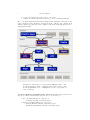
1.1. Components in the FEniCS Project. The interaction of components
within the FEniCS project is reflected in Figure 1.1. The core library is Dolfin,
which is a library written in C++ with interfaces to C++ and Python (as a module). It provides functionalities such as
•
•
•
•
mesh handling (refinement, coarsening, smoothing, partitioning),
mesh generation (currently only for simple shapes),
assembly of linear and bilinear (in general: multilinear) forms,
input/output routines
Linear algebra and visualization is handled by external software.
The typical usage of the library within a C++ program is like this:
ffc
demo.ufl −→ demo.h
demo.cpp
C++ compiler
−→
demo
In this case, the form compiler ffc (or its alternative, SyFi/SFC) generates a
header file demo.h which defines a number of problem specific classes that may be
instantiated by the user in her main program and passed to the Dolfin library.
These provide the functionality needed in the innermost loop of FE assembly routines, e.g.,
• evaluation of basis functions and their derivatives,
• application of local degrees of freedom to a function,
Date: April 1, 2011.
1
2
ROLAND HERZOG
• local-to-global mapping of the degrees of freedom,
• evaluation of the local element tensor (e.g., the local stiffness matrix).
The code which implements this functionality is automatically generated by the
form compiler from the high-level description in the .ufl file. By contrast, from
within a Python program, the form compiler is called automatically whenever necessary (just in time).
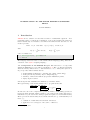
Figure 1.1. Interaction of components in FEniCS. UFL = Unified Form Language, FFC = Unified Form Compiler, UFC = Unified Form-Assembly Code. Highlighted are the components we
refer to this text.
1.2. Some Features and Limitations. FEniCS currently supports the following types of finite element function spaces (see [?, Section 4.3]):
• H 1 conforming FE spaces composed of:
– Lagrange elements of arbitrary degree
• H(div) conforming FE spaces composed of:
– Raviart-Thomas elements of arbitrary degree
– Brezzi-Douglas-Marini elements of arbitrary degree
INTRODUCTION TO FEniCS
3
– Brezzi-Douglas-Fortin-Marini elements of arbitrary degree
– Nédélec elements (1st kind) of arbitrary degree
– Nédélec elements (2nd kind) of arbitrary degree
• H(curl) conforming FE spaces composed of:
– Nédélec elements (1st kind) of arbitrary degree
– Nédélec elements (2nd kind) of arbitrary degree
• L2 conforming FE spaces composed of:
– discontinuous Lagrange elements of arbitrary degree
– Crouzeix-Raviart elements (degree one)
All of these can be used on simplicial meshes in 1D, 2D and 3D (intervals, triangles,
tetrahedra), but currently not on other geometries (rectangles, cubes, prisms etc.).
The variational form language is described in more detail in Section 3. It supports
in particular
• scalar, vector valued and matrix valued finite elements,
• integrals over cells, interior facets and exterior facets (but not over arbitrary
lines or surfaces),
• jumps and averages over facets, which can be used for error estimation and
in discontinuous Galerkin (DG) approaches.
The visualization of results is accomplished by external packages such as ParaView,
MayaVi, or Viper, which is also part of the FEniCS project.
2
Examples
The following examples conform to ffc version 0.9.4 (ffc -v) and the Dolfin
core library version 0.9.9, which are installed on the compute servers of the faculty.
Note that the interfaces to the Dolfin library are still changing slightly.
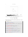
2.1. The Poisson Equation.
Purpose of this example:
• solve Poisson equation with Lagrange FEs of various degrees
• present C++ and Python interfaces
• visualize the results
• implement various choices of boundary conditions and non-constant coefficients
We consider the Poisson equation in its variational form, i.e., find u ∈ V such that
Z
Z
∇v · ∇u dx =
v f dx
Ω
Ω
for all v ∈ V = {v ∈ H 1 (Ω) : v = 0 on ΓD }, where ΓD is the Dirichlet part of the
boundary Γ = ∂Ω. In its strong form, this problem corresponds to −4u = f in Ω
with boundary conditions u = 0 on ΓD and ∂u/∂n = 0 on the complement ΓN .
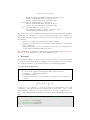
The corresponding variational description in UFL looks like this (Example_Poisson.
ufl):
element = FiniteElement ( " Lagrange " , triangle , 1)
v = TestFunction ( element )
u = TrialFunction ( element )
f = Coefficient ( element )
4
ROLAND HERZOG
a = inner ( grad ( v ) , grad ( u ) ) * dx
L = v * f * dx
We compile it using ffc and obtain a header file Example_Poisson.h.
ffc -l dolfin Example_Poisson . ufl
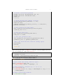
The following main program makes use of the general Dolfin classes Function,
SubDomain, UnitSquare, Constant, DirichletBC, VariationalProblem, and File.
It also uses the classes FunctionSpace, BilinearForm and LinearForm which have
been defined in the header file Example_Poisson.h, automatically generated by
ffc.
# include < dolfin .h >
# include " Example_Poisson . h "
using namespace dolfin ;
// Source term
class Source : public Expression
{
public :
Source () : Expression () {}
void eval ( Array < double >& values , const Array < double >& x
) const
{
double dx = x [0] - 0.5;
double dy = x [1] - 0.5;
values [0] = 500.0* exp ( -( dx * dx + dy * dy ) / 0.02) ;
}
};
// Subomain for Dirichlet boundary condition
class Diric hletBo undary : public SubDomain
{
bool inside ( const Array < double >& x , bool on_boundary )
const
{
return x [0] < DOLFIN_EPS or x [0] > 1.0 - DOLFIN_EPS ;
}
};
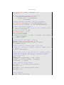
int main ()
{
// Create mesh and function space
UnitSquare mesh (32 , 32) ;
Example_Poisson :: FunctionSpace V ( mesh ) ;
// Define boundary condition
Constant u0 (0.0) ;
Dir ichlet Bounda ry boundary ;
DirichletBC bc (V , u0 , boundary ) ;
INTRODUCTION TO FEniCS
5
// Define variational problem
Example_Poisson :: BilinearForm a (V , V ) ;
Example_Poisson :: LinearForm L ( V ) ;
Source f ;
L.f = f;
// Setup problem and compute solution
Va ri at io na lP ro bl em problem (a , L , bc ) ;
Function u ( V ) ;
problem . parameters [ " linear_solver " ] = " iterative " ;
problem . solve ( u ) ;
// Save solution in VTK format
File solution_file ( " poisson_solution . pvd " ) ;
solution_file << u ;
// Save the mesh also
File mesh_file ( " poisson_mesh . xml " ) ;
mesh_file << mesh ;
// Save the parameter file
File parameter_file ( " poi ss on _p ar am et er s . xml " ) ;
parameter_file << problem . parameters ;
// Plot the mesh and the solution ( using viper )
plot ( mesh ) ;
plot ( u ) ;
return 0;
}
The we invoke the build tool CMake to obtain the executable Example_Poisson,
run it and visualize the solution with ParaView.
cmake . && make
./ Example_Poisson
paraview -- data = poisson_solution . pvd
Here is a file with the same functionality in Python:
from dolfin import *
# Create mesh and define function space
mesh = UnitSquare (32 , 32)
V = FunctionSpace ( mesh , " Lagrange " , 1)
# Define boundary condition ( x = 0 or x = 1)
u0 = Constant (0.0)
bc = DirichletBC (V , u0 , " x [0] < DOLFIN_EPS || x [0] > 1.0
- DOLFIN_EPS " )
# Define variational problem
u = TrialFunction ( V )
6
ROLAND HERZOG
v = TestFunction ( V )
f = Expression ( " 500.0* exp ( -( pow ( x [0] - 0.5 , 2) + pow ( x [1]
- 0.5 , 2) ) / 0.02) " )
a = inner ( grad ( u ) , grad ( v ) ) * dx
L = f * v * dx
# Setup problem and compute solution
problem = Va ria ti on al Pr ob le m (a , L , bc )
problem . parameters [ " linear_solver " ] = " iterative "
u = problem . solve ()
# Save solution in VTK format
solution_file = File ( " poisson_solution . pvd " )
solution_file << u
# Save the mesh also
mesh_file = File ( " poisson_mesh . xml " )
mesh_file << mesh
# Save the parameter file
parameter_file = File ( " p oi ss on _p ar am et er s . xml " )
parameter_file << problem . parameters
# Plot the mesh and the solution ( using viper )
plot ( mesh )
plot (u , interactive = True )
Execute it by saying
python -i Example_Poisson . py
where the switch -i stands for interactive mode after the script has been executed.
Changing the Boundary Conditions. We now change the problem by modifying the boundary conditions. We use u = sin(π x2 ) on ΓD , ∂u/∂n + α u = g with
α(x) ≡ 1 and g(x) = −10 x1 on the complement ΓN . Moreover, we replace −4u
2 1
by − div(A∇u) with A(x) =
.
1 2
The variational problem then becomes: Find u ∈ u0 + V such that
Z
Z
Z
Z
∇v · A · ∇u dx +
α v u ds =
v f dx +
v g ds
Ω
ΓN
Ω
ΓN
for all v ∈ V = {v ∈ H 1 (Ω) : v = 0 on ΓD }.
Here are the relevant changes to the Python code above:
# Define boundary condition
u0 = Expression ( " sin ( x [1]* pi ) " )
bc = DirichletBC (V , u0 , Di richle tBound ary () )
#
u
v
f
Define variational problem
= TrialFunction ( V )
= TestFunction ( V )
= Expression ( " 500.0* exp ( -( pow ( x [0] - 0.5 , 2) + pow ( x [1]
- 0.5 , 2) ) / 0.02) " )
INTRODUCTION TO FEniCS
7
g = Expression ( " -10.0* x [0] " )
A = as_matrix ([[2.0 , 1.0] , [1.0 , 2.0]])
alpha = Constant (1.0)
a = inner ( grad ( v ) , A * grad ( u ) ) * dx + ( alpha * v * u ) * ds
Suggestions. Change the order of the finite element. Change the setting to 3D.
Try (in Python)
help ( u )
print ( u ) ; u (0.5 ,0.5) ; u . cell () ; u . element () ; u . vector ()
. array () [0:10]
help ( V )
print ( V ) ; V . dim () ; type ( V )
help ( mesh )
print ( mesh ) ; mesh . coordinates () [0:10]; mesh . cells ()
mesh . hmax () ; mesh . num_entities (0)
in the interactive Python shell. Try also the command line tool ufl-convert.
2.2. The Stokes System.
Purpose of this example:
• introduce vector valued and compound finite elements (velocity/pressure)
• implement different boundary conditions for different components of a
system
• export finite element matrices
• import finite element meshes
We consider the Stokes system in its strong form:
−µ 4u + ∇p = f in Ω,
div u = 0
in Ω,
where u represents the velocity of a fluid with dynamic viscosity µ, and p is its
pressure. Suitable boundary conditionsRare for example u = u0 on Γ, which have
to satisfy the compatibility condition Γ u0 · n = 0. Note that the pressure is
only determined up to a constant factor in this setting. We take as a first example
Ω = (0, 1)2 with u0 = (1, 0) on the upper edge, u0 = (0, 0) elsewhere and f = (0, 0).
This problem is known as a lid-driven cavity flow. The weak formulation of the
Stokes problem is: Find (u, p) ∈ (u0 + V ) × Q such that
Z
Z
Z
Z
ds
=
v · f dx
µ
∇v : ∇u dx −
div v p dx + p v
·
~
n
|{z}
Ω
Ω
Γ
=0
Ω
Z
q div u dx = 0
Ω
1
2
2
for
R all v ∈ V =2 {v ∈ [H (Ω)] : v = 0 on Γ} and all q ∈ Q = {q ∈ L (Ω) :
∼
q dx = 0} = L (Ω)/R. The problem has a saddle point structure.
Ω
from dolfin import *
# Create mesh and define function spaces ( Taylor - Hood FE )
mesh = UnitSquare (32 , 32)
V = V e c to r F un c t io n S pa ce ( mesh , " Lagrange " , 2)
8
ROLAND HERZOG
Q = FunctionSpace ( mesh , " Lagrange " , 1)
W = V * Q
# Define Dirichlet boundary ( everywhere )
class Diric hletBo undary ( SubDomain ) :
def inside ( self , x , on_boundary ) :
return on_boundary
# Define Dirichlet boundary condition everywhere
u0 = Expression (( " x [1] >1.0 - " + str ( DOLFIN_EPS ) ," 0 " ) )
bc = DirichletBC ( W . sub (0) , u0 , Di richle tBound ary () )
# Define variational problem
(v , q ) = TestFunctions ( W ) # same as vq = TestFunction ( W ) ;
(v , q ) = split ( vq )
(u , p ) = TrialFunctions ( W )
f = Constant ((0.0 , 0.0) )
mu = Constant (1.0 e -1)
n = FacetNormal ( mesh )
a = ( mu * inner ( grad ( v ) , grad ( u ) ) - div ( v ) * p + q * div ( u ) ) * dx
+ ( p * dot (v , n ) ) * ds
L = inner (v , f ) * dx
# Setup problem and compute solution
problem = Va ria ti on al Pr ob le m (a , L , bc )
problem . parameters [ " linear_solver " ] = " direct "
U = problem . solve ()
# Split the mixed solution using a deep copy
# ( copy data instead of sharing , needed to compute norms
below )
(u , p ) = U . split ( True )
# The average value of the pressure is currently random
# since the condition \ int p dx = 0 has not yet been
# enforced . We adjust the average of p now as a post
# processing step .
int_p = p * dx
average_p = assemble ( int_p , mesh = mesh )
p_array = p . vector () . array () - average_p
p . vector () [:] = p_array
# Save solution in VTK format
ufile_pvd = File ( " stokes_velocity . pvd " )
ufile_pvd << u
pfile_pvd = File ( " stokes_pressure . pvd " )
pfile_pvd << p
# Plot solution
plot (u , title = " Velocity " )
INTRODUCTION TO FEniCS
9
plot ( sqrt ( u [0]**2+ u [1]**2) , title = " Absolute Velocity " )
plot (p , title = " Pressure " )
#
#
#
A
b
#
#
#
#
Alternatively , we can assemble the linear system
manually , which offers the possibility of exporting it
M - Files are currently not supported !
= assemble ( a )
= assemble ( L )
mfile = File (" A_before_bc . m ")
mfile << A
mfile = File (" b_before_bc . m ")
mfile << b
# Apply the Dirichlet boundary conditions and export the
# linear system again
bc . apply (A , b )
# mfile = File (" A_after_bc . m ")
# mfile << A
# mfile = File (" b_after_bc . m ")
# mfile << b
# Solve the manually assembled problem
U2 = Function ( W )
solve (A , U2 . vector () , b )
# Compute the difference ( should be zero ) of velocities
( u2 , p2 ) = U2 . split ( True )
diff = u . vector () - u2 . vector ()
print " Norm of velocity difference : %.4 e " % diff . norm ( " l2
")
# Go interactive
interactive ()
R
Note that we have not enforced the condition Ω p dx = 0, and thus the system
matrix has a kernel of dimension one. (This is handled by the linear algebra subsystem.)
Changing the Boundary Conditions. We now consider a different possibility of
specifying Dirichlet boundary conditions. Instead of using boolean indicator functions like DirichletBoundary above, one may use a MeshFunction to distinguish
various parts of the boundary. In general, a MeshFunction is a function which is
defined on the entities of a given mesh, e.g., on its cells, facets, or vertices. It can
be used for many purposes such as to represent subdomains of different material,
to mark cells for refinement, or to identify different types of boundary conditions.
10
ROLAND HERZOG
In the present situation, we follow one of the examples that came with Dolfin and
consider the following boundary conditions for the Stokes system:
u=0
on Γ0
no slip boundary
u = u0
on Γ1
inflow boundary
p=0
on Γ2
outflow boundary.
These three parts of the boundary are specified by the values {0, 1, 2} of a mesh
function. In this setting, the value of the pressure is uniquely defined, i.e., the FE
stiffness matrix is invertible.
from dolfin import *
# Load mesh and subdomains
mesh = Mesh ( " dolfin -2. xml . gz " )
subdomains = MeshFunction ( " uint " , mesh , " subdomains . xml .
gz " )
#
V
Q
W
Define function spaces
= V e c to r F un c t io n S pa ce ( mesh , " Lagrange " , 2)
= FunctionSpace ( mesh , " Lagrange " , 1)
= V * Q
# No - slip boundary condition for velocity
bc_noslip = Constant ((0 , 0) )
bc0 = DirichletBC ( W . sub (0) , bc_noslip , subdomains , 0)
# Inflow boundary condition for velocity
bc_inflow = Expression (( " - sin ( x [1]* pi ) " , " 0.0 " ) )
bc1 = DirichletBC ( W . sub (0) , bc_inflow , subdomains , 1)
# Boundary condition for pressure at outflow
bc_zero = Constant (0.0)
INTRODUCTION TO FEniCS
11
bc2 = DirichletBC ( W . sub (1) , bc_zero , subdomains , 2)
# Collect boundary conditions
bcs = [ bc0 , bc1 , bc2 ]
# Define variational problem
(v , q ) = TestFunctions ( W )
(u , p ) = TrialFunctions ( W )
f = Constant ((0 , 0) )
mu = Constant (1.0 e -3)
n = FacetNormal ( mesh )
a = ( mu * inner ( grad ( v ) , grad ( u ) ) - div ( v ) * p + q * div ( u ) ) * dx
+ ( p * dot (v , n ) ) * ds
L = inner (v , f ) * dx
# Setup problem and compute solution
problem = Va ria ti on al Pr ob le m (a , L , bcs )
problem . parameters [ " linear_solver " ] = " direct "
U = problem . solve ()
# Split the mixed solution using deep copy
# ( needed for further computation on coefficient vector )
(u , p ) = U . split ( True )
u_plot = plot ( u )
p_plot = plot ( p )
print " Norm of velocity coefficient vector : %.4 e " % u .
vector () . norm ( " l2 " )
print " Norm of pressure coefficient vector : %.4 e " % p .
vector () . norm ( " l2 " )
# Alternative assembly process with more than one
# Dirichlet boundary condition : simply use :
#
A , b = assemble_system (a , L , bcs )
# or the following :
A = assemble ( a )
b = assemble ( L )
for condition in bcs :
condition . apply (A , b )
# Solve the manually assembled problem
U2 = Function ( W )
solve (A , U2 . vector () , b )
# Compute the difference ( should be zero ) of velocities
( u2 , p2 ) = U2 . split ( True )
diff = u . vector () - u2 . vector ()
print " Norm of velocity difference : %.4 e " % diff . norm ( " l2
")
12
ROLAND HERZOG
# Extract the boundary mesh
boundary_mesh = BoundaryMesh ( mesh )
# When the boundary mesh is created , we also get two maps
# ( attached to the boundary mesh as mesh data ) named
# " cell map " and " vertex map ". They are mesh functions
# which map the cells and vertices of the boundary mesh
# to their counterparts in the original mesh .
cell_map = boundary_mesh . data () . mesh_function ( " cell map " )
# Now we can create a plottable version of the subdomains
# function ( only vertex and cell valued meshfunctions can
# be plotted in viper ) .
b o un d a ry _ s ub d o ma i n s = MeshFunction ( " uint " , boundary_mesh ,
1)
b o un d a ry _ s ub d o ma i n s . values () [:] = subdomains . values () [
cell_map . values () ]
# Plot the mesh and boundary mesh
mesh_plot = plot ( mesh , title = " Mesh " )
b oun da ry _m es h_ pl ot = plot ( boundary_mesh , title = " Boundary
Mesh " )
b o u n d a r y _ s u b d o m a i n s _ p l o t = plot ( boundary_subdomains ,
title = " Boundary Subdomains " )
# Save the boundary subdomains plot as a file
b o u n d a r y _ s u b d o m a i n s _ p l o t . write_png ( " s tokes_ subdom ains . png
")
# Save the boundary mesh ( this includes the " cell map "
and " vertex map "
# mesh data )
mesh_file = File ( " s t o k e s _ b o u n d a r y _ m e s h . xml " )
mesh_file << boundary_mesh
2.3. A Nonlinear Equation. Nonlinear equations can be solved through the use
of Newton’s method. We denote the nonlinear residual by F (u). Every Newton
step requires the solution of
J(u) δu = −F (u),
0
where J(u) = F (u) is the Jacobian of F . In the context of PDEs, F (u) is a vector
whose components are generated from a linear form L(u; v), as v ranges over all
test functions: [F (u)]i = L(vi ; u). And thus the Jacobian matrix corresponds to a
bilinear form a(·, ·) in the following sense:
[J(u) δu]i = a(vi , δu; u).
(Recall that test functions are always the first argument in a bilinear form, and trial
functions are second.) It is a particular feature of FEniCS that the Jacobian can be
generated automatically from differentiating L. This is achieved by the statement a
= derivative(L, u, du) in the code below, which solves the semilinear problem
−4u + u3 = f
u=0
in Ω
on Γ.
INTRODUCTION TO FEniCS
13
from dolfin import *
# Create mesh and define function space
mesh = UnitSquare (32 , 32)
V = FunctionSpace ( mesh , " Lagrange " , 2)
# Define Dirichlet boundary ( everywhere )
class Diric hletBo undary ( SubDomain ) :
def inside ( self , x , on_boundary ) :
return on_boundary
# Define boundary condition
u0 = Constant (0.0)
bc = DirichletBC (V , u0 , Di richle tBound ary () )
# Define the source and solution functions
f = Expression ( " 500.0* exp ( -( pow ( x [0] -0.5 ,2) + pow ( x
[1] -0.5 ,2) ) /0.02) " )
u = Function ( V )
# Define the variational problem which represents the
Newton step
v = TestFunction ( V )
du = TrialFunction ( V )
# We need to define only the nonlinear residual
L = inner ( grad ( v ) , grad ( u ) ) * dx + v * u **3* dx - v * f * dx
# since the bilinear form can be created automatically
# as the derivative of the residual L at u
a = derivative (L , u , du )
# Setup the nonlinear problem L ( u ) = 0
problem = Va ria ti on al Pr ob le m (a , L , bc , nonlinear = True )
# and solve it ; NOTE that u = problem . solve ()
# DOES NOT WORK ( no progress in iterations )
problem . solve ( u )
Note that the high level command problem.solve(u) calls the Newton solver,
and the assembly of the Jacobian and the residual is triggered automatically by
the solver. The following code shows how to achieve the same with lower level
code. We manually create the problem class SemilinearEquation, derived from the
NonlinearProblem class. Note that we need to implement the evaluation routine
of the residual F (v; u) and of the Jacobian J(v, δu; u). These consist in calling
the assemble routine and then applying the Dirichlet boundary conditions for the
Newton step. We also need to manually create the Newton solver instance.
# We now solve the same problem again , but we manually
# create the NonlinearProblem instance and the solver .
# See also demo / pde / cahn - hilliard / python / demo . py
class Se mi li ne ar Eq ua tion ( NonlinearProblem ) :
14
ROLAND HERZOG
# The constructor is defined to take all arguments we
need
def __init__ ( self , a , L , bc ) :
NonlinearProblem . __init__ ( self )
self . L = L
self . a = a
self . bc = bc
self . reset_sparsity = True
# evaluation of residual F ( x )
def F ( self , b , x ) :
assemble ( self .L , tensor = b )
self . bc . apply ( b )
# evaluation of Jacobian F ’( x )
def J ( self , A , x ) :
assemble ( self .a , tensor =A , reset_sparsity = self .
reset_sparsity )
self . bc . apply ( A )
self . reset_sparsity = False
# Define another solution function
u2 = Function ( V )
v = TestFunction ( V )
du2 = TrialFunction ( V )
# This means that we also need to define the variational
problem again
L2 = inner ( grad ( v ) , grad ( u2 ) ) * dx + v * u2 **3* dx - v * f * dx
a2 = derivative ( L2 , u2 , du2 )
# Create nonlinear problem and Newton solver
problem2 = S em il in ear Eq ua ti on ( a2 , L2 , bc )
solver = NewtonSolver ( " lu " )
solver . parameters [ " c o n v e r g e n c e _ c r i t e r i o n " ] = " incremental
"
solver . parameters [ " rel at iv e_ to le ra nc e " ] = 1e -6
# Solve the problem
solver . solve ( problem2 , u2 . vector () )
# Compare the solutions
diff = u . vector () - u2 . vector ()
print " Norm of solution difference : %.4 e " % diff . norm ( " l2
")
Suggestions. Modify the problem to include non-homogeneous boundary conditions u = g on Γ, and mixed boundary conditions.
2.4. Further Reading.
• FEniCS web site
• FEniCS tutorial [?]
• UFC specifications [?]
INTRODUCTION TO FEniCS
3
15
Overview of Unified Form Language (UFL)
According to the UFL Specification and User Manual [?], UFL is designed to express
variational forms of the following kind:
nc Z
X
a(v1 , . . . , vr ; w1 , . . . , wn ) =
Ikc (v1 , . . . , vr ; w1 , . . . , wn ) dx
+
k=1 Ωk
ne Z
X
Ike (v1 , . . . , vr ; w1 , . . . , wn ) ds
∂Ωk
+
k=1
ni Z
X
k=1
Iki (v1 , . . . , vr ; w1 , . . . , wn ) dS,
Γk
where v1 , . . . , vr are form arguments (basis functions), and w1 , . . . , wn are form
coefficients. Moreover, dx, ds and dS refer to integration over a domain Ωk , its
boundary (experior facets) ∂Ωk , or its interior facets Γk respectively.
The number r of basis functions represents the arity of the form: For instance,
bilinear forms have arity r = 2, linear forms have arity r = 1. Basis functions are
declared by the keyword BasisFunction in the UFL.
Note: When defining a multivariate form, the arguments v1 , . . . , vr are assigned in
their order of declaration, not in the order in which they appear in the form. This
means that—in a bilinear form—one should always define the test function first.
v = BasisFunction ( " Lagrange " , " triangle " , 2)
u = BasisFunction ( " Lagrange " , " triangle " , 2)
a = inner ( grad ( v ) , grad ( u ) )
However, TestFunction and TrialFunction are special instances of BasisFunction
with the property that a TestFunction will always be the first argument in a form
and a TrialFunction will always be the second argument.
Coefficients are declared by the keyword Function or the special cases Constant,
VectorConstant or TensorConstant in UFL. In Python, they can also be generated
by the Expression constructor.
In UFL one can make extensive use of index notation and tensor algebraic concepts,
but we don’t go into details here. We only mention the following operators which act
on tensors of appropriate ranks: transpose, tr (trace), dot (collapse the last axis
of the left and the first axis of the right argument), inner (collapse all axes), outer
(outer product), cross (defined only for two vectors of length), det (determinant),
dev (deviatoric part of a matrix), sym and skew (symmetric and skey symmetric
parts of a matrix), cofac (cofactor of a matrix), inv (inverse of a matrix).
Forms defining PDEs need spatial derivatives of basis functions. One may use
f = Dx (v , 2) # or equivalently
f = v . dx (2)
to denote ∂v/∂x2 for example. Useful abbreviations exist for often used compound
derivatives such as grad, div and curl. Jump and average operators for interior
facets are also defined, which are needed to solve problems with discontinuous
Galerkin (DG) function spaces.
UFL also supports differentiation with respect to user defined variables (see the
demo file HyperElasticity.ufl for an example) and differentiation with respect
to basis functions. The latter can be used, for instance to automatically generate
linearized equations (e.g., for Newton iterations).
16
A
ROLAND HERZOG
Setup Environment
Currently, FEniCS is installed on the compute servers in the following versions:
• ffc Version 0.9.4
• Dolfin Version 0.9.9
Here is how to setup the environment:
# Set environment variables
source / usr / local / FEniCS /0.9.9/ setup_fenics
References
Chemnitz University of Technology, Faculty of Mathematics, D–09107 Chemnitz, Germany
E-mail address: [email protected]
URL: http://www.tu-chemnitz.de/herzog