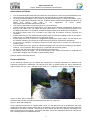
1
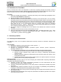
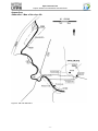
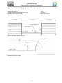
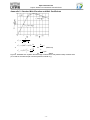
Open Channel Flow Course paper: Water level calculation with HEC-RAS Prof. Dr.-Ing. Tobias Bleninger Graduate Program for Water Resources and Environmental Engineering (PPGERHA) Universidade Federal do Paraná - UFPR Centro Politécnico, Bloco V, Caixa Postal 19011 81531-990, Curitiba - PR, Brasil Tel.: 041 - 3361 3212 Cel.: 041 - 8497 5685 [email protected] www.tobias.bleninger.info 21. junho 2015 -1- Open Channel Flow Project: Water level calculation with HEC-RAS Acknowledgements This work is based on the seminar paper developed by Markus Vaas and Nikolai Stache of the Institute for Hydromechanics of the Karlsruhe Institute of Technology (www.ifh.kit.edu), Germany. The author acknowledges their help and support and that they made the work available for teaching purposes at the UFPR. Further information on the German project can be found under: http://www.ifh.kit.edu/english/418.php Introduction The Influence of river engineering activity on the water levels is estimated by using one-dimensional simulation software. This is done to enable planning and evaluation of river engineering measures regarding navigational issues or danger of flooding and erosion. For the calculation of water surface elevations in open channels numerical models are increasingly employed, using existing real world data. These simulation models have to adequately account for the physical and geometric complexity of the watershed and have to meet the demands of river engineering in terms of accuracy and economic efficiency. For the calculation of water surface elevations in open channel flows, one-dimensional mathematical models are available. Therein the following simplifying assumptions are made: one-dimensional approach mild slope of the river bed constant roughness and linear friction slope between adjacent cross profiles rigid boundaries (no sediment transport) The one-dimensional approach is based on the energy loss in each calculation step. The individual calculation steps are each tied to a cross profile along the river. For the calculation of the energy loss HEC-RAS uses Manning’s law as a flow formula. The roughness coefficients n (“Manning’s n”, also 1/3 known as Strickler coefficient k st [m /s] = 1/n) used in this formula are taken as constant in the individual calculation steps. From the real-world geometric data of the individual cross profiles, suitable x-y-datasets have to be derived for the numerical calculation of the water surface elevations. This is done with the x-axis being defined normal to the flow direction from an arbitrary base point and the y-axis as the elevation of the cross profile point. The distances between adjacent cross profiles have to be known, too. For subcritical flow the calculation of the water surface is done stepwise against the flow direction, according to the control location concept. Hence for supercritical flow, the steps follow the flow direction. At the respective starting locations the water surface elevations have to be known as boundary conditions. A detailed discussion of the calculation of water surface elevations is provided in class or in the related literature on "Free surface flows", "Open channel flow", "Fluvial Hydrauilcs", or similar. Within the context of the project, numerical water surface calculations for two different reaches of the Alb River (see appendix 1) are done using a one-dimensional flow model. The software package HEC-RAS is used for modeling and calculation. For help on using HEC-RAS as well as documentation of the underlying mathematical model and equations employed, the manuals ’HEC-RAS User´s Manual’, ’HEC-RAS Applications Guide’ and ’HEC-RAS Hydraulic Reference Manual’ can be downloaded. The geometric data files containing the cross sections for both river reaches are also available at the course homepage (http://people.ufpr.br/~tobias.dhs/canais.htm). -2- Open Channel Flow Project: Water level calculation with HEC-RAS Instructions and Notes You can download HEC-RAS and its manuals here: http://www.hec.usace.army.mil/software/hec-ras/ The project files and geometric data files here: http://people.ufpr.br/~tobias.dhs/canais.htm) Any word processing software can be used to write the seminar paper (e.g. Word, OpenOffice, Latex) as long as a PDF file is submitted in the end. Include a table of contents and appropriate labels for all tables and figures. Also refer to the suggestions in these guides: http://people.ufpr.br/~tobias.dhs/orientacao.htm Use accuracy adequate for engineering work for your end results. Include the tabular results from HEC-RAS in your paper where required or appropriate. Within HECRAS you can define your own tables and then export them to a word processing program to be modified or extended or re-formatted. All tables and figures have to be labeled and commented. All required results have to be included in the paper and all solutions must be complete and consistent Please submit all your final HEC-RAS files together with a printed and a digital version of your paper, either on CD, on a USB flash drive or as a ZIP file by email. Please share with us any comments or suggestions regarding this project paper. You will help us and the students following you! Please tell us the total time required to complete the assignment. If you have any problems or questions, make use of the office hours or contact your supervisor by email any time You are allowed to work in groups of 2 students handing over one result and receiving a joint grade. However, copying between distinct groups is not allowed and will cause grade 0. All steps in the instruction below must be reported in the final report. All material must be in English. The final presentation of the results should also be prepared and presented in English, with a duration of approximately 15min. Have fun with the HEC-RAS project! Project definition As the planning engineer you are tasked with supplying the required verifications for different river engineering measures to authorities. The German river Alb is a medium-sized river with a watershed of approximately 457 km², and a running length of 56 km. It originates in the northern Black Forest at a height of about 750 m above sea level and enters the Rhine valley near Ettlingen. It flows through Karlsruhe and joins the river Rhine at Rhine-kilometer 367.5 (s. Figure 1). Figure 1: River Alb at Ettlingen For the planned construction of a bridge within reach A of the Alb River and for renaturation and other construction work within reach B of the river an assessment of the expected water levels and roughness distribution in this area is needed. The problem is to be solved with the aid of numeric calculations. The tasks are arranged chronologically. This means that data, results and calibrations should be carried over from preceding tasks if not stated otherwise. -3- Open Channel Flow Project: Water level calculation with HEC-RAS 1. River Reach “A” Calculation of water surface elevations and simulation of a bridge in channel reach A considering variations in channel roughness A bridge is planned across the Alb River within reach A (km 5.595 to km 8.744) at km 8.035. A numerical calculation of the water surface elevations must be done for different discharges. The effects on the water levels of a change in roughness on the overbanks and in the main channel have to be investigated, especially in the vicinity of the bridge. The downstream water surface is controlled by a stop log weir at km 5.600. It is a three-field system with weir field widths of b = 10 m (see appendix 3). The geometric data of the channel is already known. Use the supplied project file (filename: aufg-a.prj). Also contained in the file are the roughness-coefficients (Manning’s n). Note: Please create a subdirectory „part A“ in your working directory. Copy the file “aufg-a.prj” there. Use this directory for all files of part A of this assignment. 1.1. Water Surface Calculation for Mean Water 3 A water surface calculation with a mean water flow MQ = 2 m /s in channel reach A of the Alb River (km 5.595 – 8.744) is necessary to estimate mean water elevations and minimum flow velocities. Only the centre field of the stop log weir is (partially) opened, the outer fields are closed (see appendix 2). You can assume the weir to be sharp-crested and assume free flow downstream of the weir (i.e. no backwater). The weir crest of the center field is initially set to an elevation of +99.63 m for mean water flow. The 3 control water surface elevation +99.72 m at river station km 5.595 for mean water flow (MQ = 2 m /s) is known from measurements. Procedure 1. Describe the project region using the provided data, as well as information from a literature review. Note: Focus on technical information (e.g. maps and satellite images) and explore the provided data in detail to obtain for example the mean bed slope, mean river width, bed material, etc. 2. Check for criticality of the flow and determine the direction of the numerical calculation (upstream or downstream). Note: Calculate an approximate normal depth using Manning’s law. Compare with the critical depth yc. Assume a wide rectangular channel. 3. Calculate an approximate mean inclination of the water surface manually for the whole branch and all discharges as a first estimate and compare with HEC-RAS results afterwards. 4. In HEC-RAS, model the stop log weir as an inline structure using the information in appendix 2. Note: First define the outer shape of the completely closed weir as a rigid structure [Weir/Embankment] at the correct location using the geometry editor [Edit – Geometric Data – Inline Structure]. Then add the three weir fields [Gates] to this structure. Choose the right weir geometry [weir crest shape] (→ HECRAS User’s Manual p. 6-64ff). 5. Describe the principle of ineffective areas, its justification and its consequences for the solved equations using the HEC-RAS manual or additional information. 6. Define ineffective areas around the weir by adding them in the respective adjacent cross profiles. [Edit – Geometric Data – Cross Section – Options – Ineffective Flow Areas] (→ HEC-RAS User’s Manual S. 6-16). Modify those areas after the first model run to check for model sensitivity related to that schematization. 7. Iteratively calculate the overflow height at the weir for mean water flow (MQ = 2 m³/s) using appendix 3. Choose the accuracy at which to abort the iteration and substantiate your decision. 8. Create a discharge profile for the calculation with mean water flow (MQ = 2 m³/s) [Edit – Steady Flow Data]. Rename this profile to „MQ“ [Options – Edit Profile Names]. Enter the known control water surface elevation +99.72 m at river station km 5.595 as a boundary condition. Define the condition of the weir gates (left and right weir field closed, central field opened as shown in appendix 2) under [Edit – Steady Flow Data – Options – Gate Openings]. (→ HEC-RAS Users´s Manual S. 7-1ff) Calculate the water surface elevations. Note: You can change the boundary conditions with the button „Reach Boundary Conditions“ in the Steady Flow Editor. There you choose „Set boundary for one profile at a time“ and then you can define the control water surface elevation with the button „Known W.S.“ for your mean water discharge profile „MQ“. 9. Undertake a sensitivity analysis changing uncertain model parameters (e.g. ineffective areas, weir equation, boundary conditions), and quantifying their influence on model results. -4- Open Channel Flow Project: Water level calculation with HEC-RAS 10. Export a table of relevant model results (e.g. water surface elevations, depths, widths, velocities, and several more) to your paper and also add a longitudinal plot and some cross-sectional plots of the water surface elevations (→ HEC-RAS User’s Manual S. 9-1ff, S. 9-13ff). 11. Compare the calculated water level at the stop log weir with the water level obtained from your hand calculation in A.1.7. What could be the reason for a potential difference in the results? 12. Compare the calculated parameters with your hand calculations from A. 1.2 and A. 1.3. 13. Save your new geometric data [Edit – Geometric Data – File – Save Geometric Data as...] under the name „a_geo_1-3“ and your flow data [Edit – Steady Flow Data – File – Save Flow Data as...] using the name „a_flow“. 14. Compute additional parameters, such as bed shear stress, velocity profile, surface velocity, shear velocity, mean velocity profile, and profile of turbulent fluctuations for 3 arbitrary cross-sections, and compare those with each other using tables and graphs. 1.2. Water Surface Calculation for Medium Flood Water 3 In the next step calculate the water surface elevation for mean flood water flow (MHQ = 20 m /s). Vary the water depth by changing the weir height in the center field within the limits of the stop log weir so that both of these conditions are met: I To avoid sediment transport during medium flood water, maximum flow velocity must not exceed 0,75 m/s anywhere in the river reach. Note: Velocities exceeding 0.75 m/s will occur and are allowed in the immediate vicinity of the weir! II To avoid waterlogging of the soil near river station km 8.744 the water surface elevation must remain below +102.13 m. The outer fields of the weir remain closed. The control water surface elevation +100.60 m is known for 3 mean flood water flow (MHQ = 20 m /s) at km 5.595 from measurements. Procedure 3 1. Add a new discharge profile „MHQ“ with mean flood water discharge MHQ = 20 m /s and the boundary conditions given above to your discharge data. Note: To insert a new discharge profile, increase the number of profiles from 1 to 2 [„Enter/Edit Number of Profiles“] in the Steady Flow Editor and name this new profile „MHQ". Under „Reach boundary Conditions“ you can now enter the control water surface elevation for the new profile. 2. Vary the weir height in the center weir field (under [Edit – Steady Flow Data – Options – Gate Openings]) for your profile MHQ so that both conditions given above are met. (→ HEC-RAS User’s Manual S. 9-13ff). Also specify weir heights that have not worked and state which conditions were not met. Observe that each stop log has a height of 15 cm (see appendix 2). 3. Export a table of water surface elevations to your paper and also add a longitudinal plot of the water surface elevations. Note: choose the correct profile („MHQ“) for the display of the results. 4. Save your new discharge profile and the weir gate positions again under the name „a_flow“ [Edit – Steady Flow Data – File – Save Flow Data]. The geometry remains unchanged (a_geo_1-3). 1.3. Water Surface Calculation for Highest Flood Water In case of a maximum floodwater discharge HHQ = 100 m³/s all weir fields are opened completely. Because of the higher water surface elevation downstream of the weir, no free flow is possible and a backwater will occur. For this case the control water surface elevation at the downstream channel end is defined as +104.49 m. Calculate the water surface elevation for HHQ = 100 m³/s. Procedure 1. Insert a third discharge profile for HHQ = 100 m³/s in the Steady Flow Data Editor. Enter the new control water surface elevation as a boundary condition for the new profile. 2. Adjust the weir gate openings for the profile HHQ. [Edit – Steady Flow Data – Options – Gate Openings] 3. Calculate the water surface elevations. 4. Export a table of water surface elevations to your paper and also add a longitudinal plot of the water surface elevations. Note: choose the correct profile („HHQ“) for the display of the results. 5. Save your flow data again under the name „a_flow“ [Edit – Steady Flow Data – File – Save Flow Data]. 6. Compute additional parameters, such as bed shear stress, velocity profile, surface velocity, shear velocity, mean velocity profile, and profile of turbulent fluctuations for the same cross-sections for all three discharges, and compare those with each other using tables and graphs. -5- Open Channel Flow Project: Water level calculation with HEC-RAS 1.4. Simulation of a Bridge at River Station km 8,0355 At river station km 8.0355 a bridge with four piers is planned. The elevation of the bottom edge of the bridge is +104.90 m. The planned location and the geometric properties of the bridge and of the piers can be taken from appendices 4 and 5. Implement the bridge into the existing dataset. Check if in case of the maximum flood water HHQ = 100 m³/s a minimum freeboard of freq = 0.10 m under the bridge remains. Procedure: 1. Do an approximate manual calculation for the expected energy loss cause by the bridge piers, using the table and graphs provided during the class or literature values. 2. Insert the required cross profiles (→ HEC-RAS Users´s Manual S. 6-11ff). The x-y data of the additional cross profiles is given in appendix 4. 3. Model the bridge (→ HEC-RAS Users´s Manual S. 6-31ff). All required data is given in app. 5. 4. Define the ineffectice flow areas caused by the outer bridge piers and implement them for the cross profiles directly adjacent to the bridge [Edit – Geometric Data – Cross Section – Options – Ineffective Flow Areas] (→ HEC-RAS Hydraulic Reference Manual S. 5-5ff). 5. Calculate the water surface elevations with HEC-RAS twice, once with the energy equation (Bernoulli) and then with the momentum equation. (→ HEC-RAS Users´s Manual S. 6-55ff und HEC-RAS Hydraulic Reference Manual S. 5-9ff). Select one of the methods for your further calculations. Explain your decision. 6. Check if the minimum freeboard freq = 0.10 m remains. Note: You can see all data relevant to the bridge in the special “Bridge” type table under [View – Detailed Output Tables – Type – Bridge]. 7. Export a table of water surface elevations to your paper and also add a longitudinal plot of the water surface elevations. Also add an enlarged longitudinal plot for the area containing the bridge. Note: choose the correct profile („HHQ“) for the display of the results. 8. Compare the obtained results with your hand calculation for the expected energy loss. 9. Save your new geometric data under the name „a_4_geo“ [Edit – Geometric Data – File – Save Geometric Data as...] and your flow data [Edit – Steady Flow Data – File – Save Flow Data]. 1.5. Simulation of Increased Roughness on the Overbanks For ecological reasons, the effect of uncontrolled vegetation growth on the overbanks on the water surface elevations near the bridge in the case of flood water flow is to be investigated. Therefore, an increased roughness on the overbanks has to be simulated. Procedure 1. Do an approximate manual calculation for the water level increase using the equation for composite channels. 2. Change the roughness on the overbanks to a typical roughness coefficient for “light brush and trees in summer“ (→ HEC-RAS Hydraulic Reference Manual S. 3-14). 3. Check the minimum freeboard under the bridge (freq = 0.10 m). 4. Explain the result and make a statement regarding the importance of controlling growth on the overbanks. 5. Compare the obtained results with your hand calculation for the expected water level increase. 6. Save your new geometric data under the name „a_5_geo“ [Edit – Geometric Data – File – Save Geometric Data as...]. 1.6. Simulation of Increased Roughness in the Main Channel Several small floods in the area up to 1 km upstream of the stop log weir resulted in strong sediment transport. To prevent overflow of the river during floods, the channel bottom is to be excavated again. Due to the irregularities introduced by the excavation work, bottom roughness will increase in the main channel between km 5.595 und km 6.600. Check if the minimum free board freq = 0.10 m at the bridge is still met. Procedure 1. Change the roughness in the part of the main channel stated above to a typical value for a natural stream (“clean, winding, some pools and shoals“) (→ HEC-RAS Hydraulic Reference Manual S. 3-14). -6- Open Channel Flow Project: Water level calculation with HEC-RAS 2. Calculate the water surface elevations and check if the minimum freeboard f req = 0.10 m at the 3 bridge is still met for the maximum flood water HHQ = 100 m /s. 3. Compare the results of 1.5. and 1.6. in a table and or graph. 4. Interpret the differences between your results from 1.5. and 1.6. What does that mean for the excavation work in the main channel? 5. Save your new geometric data under the name „a_5_geo“ [Edit – Geometric Data – File – Save Geometric Data as...]. -7- Open Channel Flow Project: Water level calculation with HEC-RAS 2. River Reach “B” Investigation of channel reach B between river stations km 17.550 and km 20.454 Note: Please create a subdirectory „part B“ in your working directory. Copy the file aufg-b.prj there. Use this directory for all files and data of part B. 2.1. Calibration of the water surface level Because of renaturation measures along the river in reach B of the Alb River (km 17.550 – 20.454; see appendix 1) the roughness changes in this area. The energy loss calculated with the original roughnessallocation no longer complies with the natural conditions and results in wrong water level calculations. The roughness is to be calibrated with the aid of water level measurements which were obtained after the renaturation during mean water flow (MHQ = 20 m³/s). Take the measured water levels from the cross profiles in appendix 6. The channel geometry after the renaturation is contained in the file ’aufg-b.prj’. Choose reasonable roughness-coefficients and explain your choice. Procedure 1. Check for criticality again with an approximate calculation by hand and choose the correct direction for the calculations (upstream or downstream). 2. Calculate the water surface elevations for a sensibly chosen constant roughness-coefficient. (→ HEC-RAS Hydraulic Reference Manual S. 3-14). The natural river bed of the Alb River is clean and without major anomalies in this area. Take the control water surface elevations from appendix 5. Name the profile „MHQ normal“ in the Steady Flow Data Editor. 3. Vary the roughness-coefficients step-by-step moving along the cross-sections until the water level of the current channel reach agrees with the measured water levels. 4. Document the roughness-coefficients and the water levels of the individual cross-profiles in a table and compare them to the original coefficients from 1.2. 5. Interpret the new final new roughness coefficients that you just obtained. Are they reasonable and how do they compare to the original values? 6. Display a longitudinal plot of the water surface profile in your paper. 7. Save your new geometric data [Edit – Geometric Data – File – Save Geometric Data as...] under the name „b_1_geo“ and your flow data [Edit – Steady Flow Data – File – Save Flow Data as...] using the name „b_flow“. 2.2. Backwater Curve Calculation Because of construction work a constriction of the channel is introduced in river reach B at river station km 17.500. The reduction of the channel width induces an increase of the water surface level at the cross section km 17.550 of about 0.10 m during mean water discharge (MHQ = 20 m³/s). Determine the backwater limit or stagnation point, i.e. how far upstream the increase of the water level at km 17.550 has an effect on the water surface level. Procedure 1. Check for criticality again as before. 2. Insert a second profile in the Steady Flow Data Editor, containing the modified control water surface elevation at km 17.550 as a boundary condition. Name this profile „MHQ constricted“. 3. Insert interpolated cross profiles with a maximum distance of 20 m in the channel reach between km 17.550 and km 19.000 (→ HEC-RAS Users´s Manual S. 6-102ff). 4. Calculate and compare the water surface elevations before and after the building activity. Show both water surface profiles in a comparison table. Insert a column which displays the difference of the water surface elevations before and after the building activity. 5. Display the course of the water level before and after the building activity in a longitudinal profile plot. 6. Determine the location of the stagnation point and show it in an enlarged profile plot. 7. Explain the advantage of using interpolated cross sections in this case. 8. Save your flow data [Edit – Steady Flow Data – File – Save Flow Data] under the name „b_flow“. 9. Calculate the backwater curve manually (or using an own code) by using the single-step method and using a unique simplified profile and compare with the HEC-RAS data and discuss the results. -8- Open Channel Flow Project: Water level calculation with HEC-RAS 2.3. Calculation of a Flood Wave Due to an intense rain event in the watershed ,a flood wave is passing through the Alb River. Check if river reach “B” offers the necessary capacity to convey the temporarily increased discharge volume. Note: 3 Reach B already carries the mean water flow MHQ = 20 m /s when the wave occurs! Procedure 1. Enter the unsteady flow data [Edit – Unsteady Flow Data]. Use the discharge hydrograph of the flood water at km 20.454 from appendix 7. 2. Run the simulation for the given time period. 3. Determine whether the flow remains within the maximum cross sectional area. If not so, identify the flooded sections and calculate the time period of flooding for one of these cross sections. Add a table and cross-sectional plot as well as a plot of the water level over time at that section. Mark the water level at which the flooding occurs. Note: For the analysis of unsteady discharge HECRAS needs the list of the cross-sections where the unsteady water levels are calculated [Unsteady flow analysis – Options – Stage and flow output locations] (By default only the results from upstream and downstream limits are shown). 4. Up to which height do sandbags have to be stacked at the affected river sections to prevent flooding? 5. Calculate the speed at which the wave travels down the river. 6. Save your flow data under the name „b_unstd_flow“ [Edit – Unsteady Flow Data – File – Save Unsteady Flow Data as…] and your calculation plan under [Run – Unsteady Flow Analysis – File – Save Plan as...] with the name „b_3_plan“. 3. Laboratory studies 3.1. Lab-setup and measurements The laboratory setup, and the applied measurement technique should be described, analyzed and evaluated. Lab procedure 1. Describe the laboratory setup (geometries, scales, pictures, …) 2. Describe the measurement techniques 3. Describe the measurement program (coordinate system, locations, periods, frequencies, boundary conditions, etc.) 4. The following steps should be done for two different discharges and interchanging groups: a. Determine the total flow using the flow meter of the lab and approximate equations. b. Measure surface velocities using confetti and running a statistically representative number of tests. c. Measure velocities at different characteristical points (at least 6) within the channel, using the propeller flow meter. d. Measure at least three vertical velocity profiles (close to the previous points, and using at least 4 points for each profile) using the ADV. Office procedure The following steps should be done in the office analyzing the obtained data comparing characteristic parameters with theoretical equations: 5. Calculate, compare, and analyze characteristic parameters for each measurement and each measurement point (mean, standard deviation, …) 6. Calculate characteristic parameters for each profil (vertical, horizontal) and visualize the profiles and values. 7. Add theoretically determined profiles to the plot, and compare / fit qualitatively and quantitatively including the measurements from the propeller and the confetti. 8. Calculate the total mean velocity and the total discharge and compare with theoretical values and the measured value. 9. Calculate the theoretical water level using Darcy-Weissbach and Manning equation and compare with measured water levels. -9- Open Channel Flow Project: Water level calculation with HEC-RAS 4. Technical Report Write a technical report taking into account all results of parts 1 to 3 for submission to local authorities. The report herefore should also contain information on: project region, description of river and available data objectives of the study compilation, description, and discussion of available data description of governing equations and numerical scheme and software implementation description and analysis of simulation results statistical analysis of obtained results sensitivity analysis conclusions - 10 - Open Channel Flow Project: Water level calculation with HEC-RAS Appendices Appendix 1: Map of the river Alb Figure 2: Alb near Karlsruhe - 11 - Open Channel Flow Project: Water level calculation with HEC-RAS Appendix 2: Details on the geometry of the stop log weir Thickness of the stop logs: Height of the stop logs: Centerline location of the stop log weir is at: Boundary of the outer weir fields : Upper edge of the closed outer weir fields : 0.10 m 0.15 m km 5.600 20.0 m and 30.0 m +102.00 m Figure 3: geometric details of the weir Figure 4: cross section view of the stop log weir and schematic definition of overfall height, weir height and spillway approach height - 12 - Open Channel Flow Project: Water level calculation with HEC-RAS Appendix 3: Standard Weir Equation and Weir Coefficients CQ 1. q 2 g h0 3 2 CQ 0,407 0,053 2. w CQ 0,707 1 h0 h0 w h0 for w 6 (Rehbock) 32 w 0,06 h0 3. for (Böss) Figure 5: Standard weir equation and discharge coefficients for fully aerated sharp-crested weirs (h is used for the water depth in these equations instead of y). - 13 - Open Channel Flow Project: Water level calculation with HEC-RAS Appendix 4: Table of the cross profiles for the planned installation of the bridge at km 8.0355 Profile 8,030 x y -4,0 105,47 0,0 103,48 0,01 103,47 5,3 103,29 7,6 102,33 8,0 102,12 8,1 102,11 9,1 101,48 10,6 100,62 10,6 100,61 12,2 100,29 13,7 100,32 14,2 100,32 15,2 100,28 16,3 100,23 16,8 100,21 18,4 100,16 20,3 100,22 21,3 100,21 22,2 100,20 24,2 100,24 24,4 100,27 26,6 100,68 26,7 100,71 27,3 101,10 29,0 102,09 29,0 102,11 31,9 103,33 37,2 103,43 37,2 103,45 41,2 105,43 Profile 8,041 x y -4,0 105,47 0,0 103,48 0,01 103,47 5,3 103,29 7,6 102,32 8,1 102,11 8,1 102,09 9,2 101,46 10,7 100,61 10,7 100,6 12,2 100,29 13,8 100,32 14,3 100,32 15,3 100,28 16,4 100,23 16,9 100,21 18,5 100,16 20,4 100,22 21,4 100,21 22,3 100,21 24,2 100,25 24,4 100,28 26,7 100,71 26,7 100,74 27,4 101,14 29,0 102,10 29,0 102,13 31,9 103,33 37,2 103,43 37,2 103,45 41,2 105,43 Profile 8,050 x y -4,0 105,47 0,0 103,48 0,01 103,47 5,3 103,29 7,6 102,31 8,1 102,09 9,2 101,44 10,7 100,59 12,3 100,29 13,9 100,32 14,4 100,32 15,4 100,28 16,5 100,23 17,0 100,21 18,6 100,16 20,5 100,22 21,5 100,21 22,4 100,21 24,3 100,26 24,5 100,29 26,7 100,74 27,4 101,17 29,0 102,12 31,9 103,33 37,2 103,43 37,2 103,45 41,2 105,43 Appendix 5: Geometric Details for the planned bridge Width of the bridge: The centre of the Bridge is at (equates to “River Station” of the bridge): 10.00 m Km 8.0355 Boundary of the outside piers at „Station“: Symmetry axis of the inside piers at „Station“: Width of the inside pillars: Up to elevation +101.00 m: Up to underside of the bridge: shape of the piers 3.50 and 33.50 m 13.50 and 23.50 m Thickness of the inside pillars: 2m 1m Square profile with semi circular ends (see HEC-RAS Hydraulic Reference Manual Page 5-13) - 14 - Open Channel Flow Project: Water level calculation with HEC-RAS Höhenlage[m] 106 105 104 103 Sohle 102 Begrenzungdes Totwasserbereichs 101 Beginndes Vorlands 100 -10 0 10 20 30 40 50 Station[m] Appendix 6: Measured water levels Measured water levels between river station km 17.550 and km 20.454 during mean water discharge MHQ = 20 m³/s. The sections between these cross profiles can be considered as areas of linear roughness grade. River Station [km] 17.550 17.880 18.182 18.510 19.000 19.965 20.454 Q 3 [m /s] 20 20 20 20 20 20 20 Water surface Manning’s n elevation 1/3 [m] [s/m ] 109.86 ? 110.17 ? 110.39 ? 110.67 ? 111.07 ? 111.90 ? 112.50 ? - 15 - Open Channel Flow Project: Water level calculation with HEC-RAS Appendix 7: Unsteady discharge th th On Feb 12 and 13 following flow rates were measured at km 20.454: 12.02. time discharge Q [m3/s] [hh:mm] 00:00 20 01:00 20 02:00 20 03:00 20 04:00 20 05:00 20 06:00 20 07:00 20,5 08:00 21 09:00 22 10:00 23 11:00 24 12:00 25 13:00 26 14:00 26,5 15:00 27 16:00 27 17:00 27 18:00 27,5 19:00 28 20:00 28 21:00 28,5 22:00 29 23:00 29 00:00 29,5 13.02. time discharge Q [m3/s] [hh:mm] 01:00 30 02:00 31 03:00 31 04:00 33 05:00 33,5 06:00 34 07:00 34,5 08:00 34 09:00 33,5 10:00 27 11:00 26 12:00 25,5 13:00 25 14:00 25 15:00 25 16:00 25 17:00 24,5 18:00 24 19:00 23,5 20:00 23 21:00 23 22:00 23 23:00 23 00:00 23 - 16 -