Download pdf file

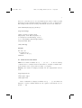
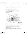
June 12, 2006
14:27
WSPC - Proceedings Trim Size: 9in x 6in
ws-procs9x6
1
FOR PROCEEDINGS CONTRIBUTORS:
USING WORLD SCIENTIFIC’S WS-PROCS9X6
DOCUMENT CLASS IN LATEX2e
A. B. AUTHOR∗ and C. D. AUTHOR
University Department, University Name,
City, State ZIP/Zone, Country
∗ E-mail: ab [email protected]
www.university name.edu
A. N. AUTHOR
Group, Laboratory, Street,
City, State ZIP/Zone, Country
E-mail: an [email protected]
This article explains how to use World Scientific’s ws-procs9x6 document class
written in LATEX2e. This article was typeset using ws-procs9x6.cls and may be
used as a template for your contribution.
Keywords: Style file; LATEX; Proceedings; World Scientific Publishing.
1. Using Other Packages
The class file loads the packages amsfonts, amsmath, amssymb,
chapterbib, cite, dcolumn, epsfig, rotating and url at startup.
Please try to limit your use of additional packages as they often introduce incompatibilities. This problem is not specific to the WSPC styles; it
is a general LATEX problem. Check this article to see whether the required
functionality is already provided by the WSPC class file. If you do need additional packages, send them along with the paper. In general, you should
use standard LATEX commands as much as possible.
2. Layout
In order to facilitate our processing of your article, please give easily
identifiable structure to the various parts of the text by making use of
the usual LATEX commands or by using your own commands defined in
June 12, 2006
14:27
WSPC - Proceedings Trim Size: 9in x 6in
ws-procs9x6
2
the preamble, rather than by using explicit layout commands, such as
\hspace, \vspace, \large, \centering, etc. Also, do not redefine the
page-layout parameters. For more information on layout and font specifications, please refer to our Layout and Font Specification Guide.
3. User Defined Macros
User defined macros should be placed in the preamble of the article,
and not at any other place in the document. Such private definitions,
i.e. definitions made using the commands \newcommand, \renewcommand,
\newenvironment or \renewenvironment, should be used with great care.
Sensible, restricted usage of private definitions is encouraged. Large macro
packages and definitions that are not used in this example article should be
avoided. Please do not change the existing environments, commands and
other standard parts of LATEX.
4. Using WS-procs9x6
You can obtain these files from the following website: http:
//eproceedings.worldscinet.com/authors.shtml, http://www.wspc.
com.sg/style/proceedings_style.shtml and http://www.icpress.co.
uk/authors/stylefiles.shtml#proceedings.
4.1. Input used to produce this paper
\documentclass{ws-procs9x6}
\begin{document}
\title{FOR PROCEEDINGS CONTRIBUTORS: ...}
\author{A. B. AUTHOR$^*$ and C. D. AUTHOR}
\address{University Department, ...}
\begin{abstract}
This article explains how to ...
\end{abstract}
\keywords{Style file; \LaTeX, ...}
\bodymatter
\section{Using Other Packages}
The class file has ...
\bibliographystyle{ws-procs9x6}
\bibliography{ws-pro-sample}
\end{document}
June 12, 2006
14:27
WSPC - Proceedings Trim Size: 9in x 6in
ws-procs9x6
3
5. Sectional Units
Sectional units are obtained in the usual way, i.e. with the LATEX commands
\section, \subsection, \subsubsection and \paragraph.
6. Section
This is just an example.
6.1. Subsection
This is just an example.
6.1.1. Subsubsection
This is just an example.
Paragraph This is just an example.
Unnumbered Section
Unnumbered sections can be obtained by using \section*.
7. Lists of Items
Lists are broadly classified into four major categories that can randomly be
used as desired by the author:
(a)
(b)
(c)
(d)
Numbered list.
Lettered list.
Unnumbered list.
Bulleted list.
7.1. Numbered and lettered list
(1) The \begin{arabiclist}[] command is used for the arabic number
list (arabic numbers appearing within parenthesis), e.g., (1), (2), etc.
(2) The \begin{romanlist}[] command is used for the roman number
list (roman numbers appearing within parenthesis), e.g., (i), (ii), etc.
(3) The \begin{Romanlist}[] command is used for the cap roman
number list (cap roman numbers appearing within parenthesis), e.g.,
(I), (II), etc.
June 12, 2006
14:27
WSPC - Proceedings Trim Size: 9in x 6in
ws-procs9x6
4
(4) The \begin{alphlist}[] command is used for the alphabetic list (alphabets appearing within parenthesis), e.g., (a), (b), etc.
(5) The \begin{Alphlist}[] command is used for the cap alphabetic list
(cap alphabets appearing within parenthesis), e.g., (A), (B), etc.
Note: For all the above mentioned lists (with the exception of alphabetic
list), it is obligatory to enter the last entry’s number in the list within the
square bracket, to enable unit alignment.
7.2. Bulleted and unnumbered list
The \begin{itemlist} command is used for the bulleted list.
The \begin{unnumlist} command is used for creating the unnumbered list with the turnovers hangindent by 1 pica.
Lists may be laid out with each item marked by a dot:
• item one
• item two
• item three.
Items may also be numbered with lowercase Roman numerals:
(i) item one
(ii) item two
(a) lists within lists can be numbered with lowercase Roman letters
(b) second item.
(iii) item three
(iv) item four.
8. Theorems and Definitions
Input:
\begin{theorem}
We have $\# H^2 (M \supset N) < \infty$ for an inclusion ...
\end{theorem}
Output:
Theorem 8.1. We have #H 2 (M ⊃ N ) < ∞ for an inclusion M ⊃ N of
factors of finite index.
June 12, 2006
14:27
WSPC - Proceedings Trim Size: 9in x 6in
ws-procs9x6
5
Input:
\begin{theorem}[Longo, 1998]
For a given $Q$-system...
\[
N = \{x \in N; T x = \gamma (x) T, T x^* = \gamma (x^*) T\},
\]
and $E_\Xi (\cdot) = T^* \gamma (\cdot) T$ gives ...
\end{theorem}
Output:
Theorem 8.2 (Longo, 1998). For a given Q-system...
N = {x ∈ N ; T x = γ(x)T, T x∗ = γ(x∗ )T },
and EΞ (·) = T ∗ γ(·)T gives a conditional expectation onto N .
The following environments are available by default with WSPC document styles:
Environment
Heading
Sample output
algorithm
answer
assertion
assumption
case
claim
comment
condition
conjecture
convention
corollary
criterion
definition
example
lemma
notation
note
observation
problem
proposition
question
remark
solution
step
summary
theorem
Algorithm
Answer
Assertion
Assumption
Case
Claim
Comment
Condition
Conjecture
Convention
Corollary
Criterion
Definition
Example
Lemma
Notation
Note
Observation
Problem
Proposition
Question
Remark
Solution
Step
Summary
Theorem
Algorithm 1.1. This is a test.
Answer 1.1. This is a test.
Assertion 1.1. This is a test.
Assumption 1.1. This is a test.
Case 1.1. This is a test.
Claim 1.1. This is a test.
Comment 1.1. This is a test.
Condition 1.1. This is a test.
Conjecture 1.1. This is a test.
Convention 1.1. This is a test.
Corollary 1.1. This is a test.
Criterion 1.1. This is a test.
Definition 1.1. This is a test.
Example 1.1. This is a test.
Lemma 1.1. This is a test.
Notation 1.1. This is a test.
Note 1.1. This is a test.
Observation 1.1. This is a test.
Problem 1.1. This is a test.
Proposition 1.1. This is a test.
Question 1.1. This is a test.
Remark 1.1. This is a test.
Solution 1.1. This is a test.
Step 1.1. This is a test.
Summary 1.1. This is a test.
Theorem 1.1. This is a test.
June 12, 2006
14:27
WSPC - Proceedings Trim Size: 9in x 6in
ws-procs9x6
6
LATEX provides \newtheorem to create new theorem environments. To
add theorem-type environments to an article, use
\newtheorem{example}{Example}[section]
\let\Examplefont\upshape
\def\Exampleheadfont{\bfseries}
\begin{example}
We have $\# H^2 (M \supset N) < ...
\end{example}
For details see the LATEX user manual.1,2
8.1. Proofs
The WSPC document styles also provide a predefined proof environment
for proofs. The proof environment produces the heading ‘Proof’ with appropriate spacing and punctuation. It also appends a ‘Q.E.D.’ symbol, ¤,
at the end of a proof, e.g.,
\begin{proof}
This is just an example.
\end{proof}
to produce
Proof. This is just an example.
The proof environment takes an argument in curly braces, which allows
you to substitute a different name for the standard ‘Proof’. If you want to
display, ‘Proof of Lemma’, then write e.g.
\begin{proof}[Proof of Lemma]
This is just an example.
\end{proof}
produces
Proof of Lemma. This is just an example.
9. Programs and Algorithms
Fragments of computer programs and descriptions of algorithms should be
prepared as if they were normal text. Use the same fonts for keywords, vari-
June 12, 2006
14:27
WSPC - Proceedings Trim Size: 9in x 6in
ws-procs9x6
7
ables, etc., as in the text; do not use small typeface sizes to make program
fragments and algorithms fit within the margins set by the document style.
An example with only the tabbing environment and one new definition:
\newcommand{\keyw}[1]{{\bf #1}}
\begin{tabbing}
\quad \=\quad \=\quad \kill
\keyw{for} each $x$ \keyw{do} \\
\> \keyw{if} extension$(p, x)$ \\
\> \> \keyw{then} $E:=E\cup\{x\}$\\
\keyw{return} $E$
\end{tabbing}
Output:
for each x do
if extension(p, x)
then E := E ∪ {x}
return E
10. Mathematical Formulas
Inline: For in-line formulas use \( ... \) or $ ... $. Avoid built-up
constructions, for example fractions and matrices, in in-line formulas. Fractions in inline can be typed with a solidus, e.g. x+y/z=0.
Display: For numbered display formulas, use the displaymath environment:
\begin{equation}
...
\label{aba:eqno}
\end{equation}
And for unnumbered display formulas, use \[ ... \]. For numbered
displayed, one-line formulas always use the equation environment. Do not
use $$ ... $$.
June 12, 2006
14:27
WSPC - Proceedings Trim Size: 9in x 6in
ws-procs9x6
8
For example, the input for:
∞
P
µ(n, t) =
i=1
1(di < t, N (di ) = n)
Rt
.
(1)
1(N (σ) = n)dσ
σ=0
is:
\begin{equation}
\mu(n, t) =
\frac{\sum\limits^\infty_{i=1}1 (d_i < t, N(d_i) = n)}
{\int\limits^t_{\sigma=0}1 (N(\sigma)=n)d\sigma}.\label{aba:eq1}
\end{equation}
For displayed multi-line formulas, use the eqnarray environment. For
example,
\begin{eqnarray}
\zeta\mapsto\hat{\zeta}&=&a\zeta+b\eta\label{aba:appeq2}\\
\eta\mapsto\hat{\eta}&=&c\zeta+d\eta\label{aba:appeq3}
\end{eqnarray}
produces:
ζ 7→ ζ̂ = aζ + bη
(2)
η 7→ η̂ = cζ + dη
(3)
Superscripts and subscripts that are words or abbreviations, as in σlow ,
should be typed as roman letters, with \(\sigma_{\mathrm{low}}\) instead of σlow done with \(\sigma_{low}\).
For geometric functions, e.g. exp, sin, cos, tan, etc., please use the
macros \sin, \cos, \tan. These macros give proper spacing in mathematical formulas.
It is also possible to use the AMS-LATEX package,2 which can be obtained from the AMS and various TEX archives.
11. Floats
11.1. Tables
Put tables and figures in text using the table and figure environments, and
position them near the first reference of the table or figure in the text.
Please avoid long captions in figures and tables.
June 12, 2006
14:27
WSPC - Proceedings Trim Size: 9in x 6in
ws-procs9x6
9
Input:
\begin{table}
\tbl{Comparison of acoustic for frequencies for piston-cylinder
problem.}
{\begin{tabular}{@{}cccc@{}}\toprule
Piston mass & Analytical frequency & TRIA6-$S_1$ model & ...\\
& (Rad/s) & (Rad/s) \\\colrule
1.0\hphantom{00}&\hphantom{0}281.0&\hphantom{0}280.81&0.07 \\
0.1\hphantom{00}&\hphantom{0}876.0&\hphantom{0}875.74&0.03 \\
0.01\hphantom{0}&2441.0&2441.0\hphantom{0}&0.0\hphantom{0} \\
0.001 & 4130.0 & 4129.3\hphantom{0}& 0.16\\\botrule
\end{tabular}}
\begin{tabnote}
$^{\text a}$ Sample table footnote.\\
\end{tabnote}\label{aba:tbl1}
\end{table}
Output:
Table 1. Comparison of acoustic for frequencies for piston-cylinder
problem.
Piston mass
Analytical frequency
(Rad/s)
TRIA6-S1 model
(Rad/s)
% Errora
1.0
0.1
0.01
0.001
281.0
876.0
2441.0
4130.0
280.81
875.74
2441.0
4129.3
0.07
0.03
0.0
0.16
Note:
a
Sample table footnote.
Very large figures and tables should be placed on a separate page by
themselves. Landscape tables and figures can be typeset with the following
environments:
• sidewaystable and
• sidewaysfigure.
Example:
\begin{sidewaystable}
\tbl{Positive values of ...}
2
0.2
5
3
0.1
1
5
0.001
0.001
0.1
1
0.1
0.1
0.1
1
5
0.2
10
2
0.001
0.001
0.51
0.302
−0.301
0.2
0.1
0.333
−0.1
0.1
0.1
0.034
−0.033
α0
0.128192
0.089435
0.128966
0.089441
0.309739,
0.275856
0.316014,
0.41436
0.414324
0.169063,
0.414412
0.19718,
0.089409
—
0.414489
0.848544,
—
—
0.466499
—
—
—
—
1.22434
2.44524,
7D
0.41436
0.089435
—
0.414412
0.91379,
—
—
0.466489
—
—
—
—
1.1879
3.15991,
6D
0.414489
0.142103,
0.08935
—
0.414605
0.783787,
—
—
0.464947
—
—
—
—
1.29065
1.92883,
8D
—
0.089061
—
0.415056
0.669541,
—
—
0.45438
—
—
—
—
0.415056
0.669541,
10D
—
0.088347
—
0.416214
0.577489,
—
—
0.429651
—
—
—
—
—
12D
—
0.084352
—
—
—
—
0.35278
—
—
—
—
—
16D
WSPC - Proceedings Trim Size: 9in x 6in
0.275327
0.968869,
—
—
0.996033,
—
—
0.465426
0.858211
0.463679
0.806578
—
1.1946
1.667,
—
1.65625
—
1.48602
1.24003
2.07773,
1.72737,
3.15662,
4.32936,
1.16321
6.75507,
5D
1.14476
4D
Positive roots (X0 )
14:27
−0.5
λ0
f0
Table 2. Positive values of X0 by eliminating Q0 from Eqs. (15) and (16) for different values of the parameters f0 , λ0 and α0
in various dimension.
June 12, 2006
ws-procs9x6
10
June 12, 2006
14:27
WSPC - Proceedings Trim Size: 9in x 6in
ws-procs9x6
11
{\begin{tabular}{@{}ccccccccccc@{}}
\toprule\\
$f_0$ &$\lambda_0$ &$\alpha_0$...
\end{tabular}}
\label{aba:tbl2}
\end{sidewaystable}
By using \tbl command in table environment, long captions will be justified to the table width while the short or single line captions are centered.
\tbl{table caption}{tabullar environment}.
For most tables, the horizontal rules are obtained by:
toprule one rule at the top
colrule one rule separating column heads from
data cells
botrule one bottom rule
Hline
one thick rule at the top and bottom of
the tables with multiple column heads
To avoid the rules sticking out at either end of the table, add @{} before
the first and after the last descriptors, e.g. @llll@. Please avoid vertical
rules in tables. But if you think the vertical rule is a must, you can use the
standard LATEX tabular environment.
Headings which span for more than one column should be set using
\multicolumn{#1}{#2}{#3} where #1 is the number of columns to be
spanned, #2 is the argument for the alignment of the column head which
may be either c — for center alignment; l — for left alignment; or r — for
right alignment, as desired by the users. Use c for column heads as this is
the WS style and #3 is the heading.
For the footnotes in the table environment the command is
{\begin{tabnote}<text>\end{tabnote}}.
Tables should have a uniform style throughout the proceedings volume.
It does not matter how you place the inner lines of the table, but we would
prefer the border lines to be of the style as shown in our sample tables. For
the inner lines of the table, it looks better if they are kept to a minimum.
11.2. Figures
The preferred graphics formats are TIF and Encapsulated PostScript (EPS)
for any type of image. Our TEX installation requires EPS, but we can easily
convert TIF to EPS. Many other formats, e.g. PICT (Macintosh), WMF
(Windows) and various proprietary formats, are not suitable. Even if we
June 12, 2006
14:27
WSPC - Proceedings Trim Size: 9in x 6in
ws-procs9x6
12
can read such files, there is no guarantee that they will look the same on
our systems as on yours.
A figure is obtained with the following commands:
\begin{figure}
\psfig{file=procs-fig1.eps,width=4.5in}
\caption{The bifurcating response curves of system
$\alpha=0.5, \beta=1.8; \delta=0.2, \gamma=0$: (a)
$\mu=-1.3$; and (b) $\mu=0.3$.}
\label{aba:fig1}
\end{figure}
Caring for other people's needs
A1
Achievement and target oriented
6
A21
A2
Polite/ courteous
Decisive
A20
Optimistic A19
5
A3 Conscientious and take care
when doing work
4
A4 Control over emotion
3
Sociable
A18
A5 Willing to adapt to or accept new/
different ideas/ situations
2
1
Critical
A6
A17
Aggressive
0
Independent
A7 Dedication to work
A16
Confident
A8 Interested & enthusiastic
A15
Realistic
A14
Risk taking
A9
A13
A12
Instinctive
Inventive
A10 Principled
A11
Investigative
Benchmark
Individual's
Fig. 1. The bifurcating response curves of system α = 0.5, β = 1.8; δ = 0.2, γ = 0: (a)
µ = −1.3; and (b) µ = 0.3.
Adjust the scaling of the figure until it is correctly positioned, and remove the declarations of the lines and any anomalous spacing.
12. Cross-references
Use \label and \ref for cross-references to equations, figures, tables, sections, subsections, etc., instead of plain numbers. Every numbered part to
June 12, 2006
14:27
WSPC - Proceedings Trim Size: 9in x 6in
ws-procs9x6
13
which one wants to refer, should be labeled with the instruction \label.
For example:
\begin{equation}
\mu(n, t) =
\frac{\sum\limits^\infty_{i=1}1 (d_i < t, N(d_i) = n)}
{\int\limits^t_{\sigma=0}1 (N(\sigma)=n)d\sigma}.\label{aba:eq1}
\end{equation}
With the instruction \ref one can refer to a numbered part that has been
labeled:
..., see also Eq. (\ref{aba:eq1})
The \label instruction should be typed
• immediately after (or one line below), but not inside the argument of
a number-generating instruction such as \section or \caption, e.g.:
\caption{ ... caption ... }\label{aba:fig1}.
• roughly in the position where the number appears, in environments
such as an equation,
• labels should be unique, e.g., equation 1 can be labeled as
\label{aba:eq1}, where ‘aba’ is author’s initial and ‘eq1’ the equation number.
Some useful shortcut commands.
Shortcut
command
Equivalent
TEX command
Output
In the middle of a sentence:
\eref{aba:eq1}
Eq. (\ref{aba:eq1})
\sref{aba:sec1} Sec. \ref{aba:sec1}
\fref{aba:fig1} Fig. \ref{aba:fig1}
\tref{aba:tbl1} Table \ref{aba:tbl1}
Eq. (1)
Sec. 1
Fig. 1
Table 1
At the starting of a sentence:
\Eref{aba:eq1}
Equation (\ref{aba:eq1})
\Sref{aba:sec1} Section \ref{aba:sec1}
\Fref{aba:fig1} Figure \ref{aba:fig1}
\Tref{aba:tbl1} Table \ref{aba:tbl1}
Equation (1)
Section 1
Figure 1
Table 1
13. Citations
We have used \bibitem to produce the bibliography. Citations in the text
use the labels defined in the bibitem declaration, e.g., the first paper by Jarlskog3 is cited using the command \cite{jarl88}. Bibitem labels should
June 12, 2006
14:27
WSPC - Proceedings Trim Size: 9in x 6in
ws-procs9x6
14
be unique.
For multiple citations, do not use \cite{1}, \cite{2}, but use
\cite{1,2} instead.
When the reference forms part of the sentence, it should not be
typed in superscripts, e.g.: “One can show from Ref. 3 that . . .”, “See
Refs. 1 and 2 for more details.” This is done using the LATEX command:
“Ref.~\refcite{name}”.
14. Footnotes
Footnotes are denoted by a Roman letter superscript in the text. Footnotes
can be used as
Input:
... total.\footnote{Sample footnote text.}
Output:
... in total.a
15. Acknowledgments and Appendices
Acknowledgments to funding bodies etc. may be placed in a separate section
at the end of the text, before the Appendices. This should not be numbered,
so use \section*{Acknowledgments}.
It is preferable to have no appendices in a short article, but if it is
necessary, then simply use as
\appendix{About the Appendix}
Appendices should be...
\begin{equation}
\mu(n, t) = \frac{\sum^\infty_{i=1} 1(d_i < t, N(d_i) = n)}
{\int^t_{\sigma=0} 1(N(\sigma) = n)d\sigma}. \label{aba:app1}
\end{equation}
\subappendix{Appendix Sectional Units}
Sectional units are...
16. References
References are to be listed in the order cited in the text in Arabic numerals.
BIBTEX users, please use our bibliography style file ws-procs9x6.bst for
a Sample
footnote text.
June 12, 2006
14:27
WSPC - Proceedings Trim Size: 9in x 6in
ws-procs9x6
15
references. Non BIBTEX users can list down their references in the following
pattern.
\begin{thebibliography}{9}
\bibitem{jarl88} C. Jarlskog, in {\it CP Violation} (World
Scientific, Singapore, 1988).
\bibitem{lamp94} L. Lamport, {\it \LaTeX, A Document
Preparation System}, 2nd edition (Addison-Wesley,
Reading, Massachusetts, 1994).
\bibitem{ams04} \AmS-\LaTeX{} Version 2 User’s Guide (American
Mathematical Society, Providence, 2004).
\bibitem{best03} B.~W. Bestbury, {\em J. Phys. A} {\bf 36},
1947 (2003).
\end{thebibliography}
17. BIBTEXing
Sample output using ws-procs9x6 bibliography style file:
BIBTEX
Database
entry type
article
proceedings
inproceedings
book
edition
editor
series
tech report
unpublished
phd thesis
masters thesis
incollection
misc
Sample citation
... text.4–6
... text.7
... text.8
... text.3,9
... text.10
... text.11
... text.12
See Refs. 13 and 14 for more details
... text.15
... text.16
... text.17
... text.18
... text.19
If you use the BIBTEX program to maintain your bibliography, you do
not use the thebibliography environment. Instead, you should include
\bibliographystyle{ws-procs9x6}
\bibliography{ws-pro-sample}
June 12, 2006
14:27
WSPC - Proceedings Trim Size: 9in x 6in
ws-procs9x6
16
where ws-procs9x6 refers to a file ws-procs9x6.bst, which defines how
your references will look.
The argument to \bibliography refers to the file ws-pro-sample.bib,
which should contain your database in BIBTEX format. Only the entries
referred to via \cite will be listed in the bibliography.
Appendix A. About the Appendix
Appendices should be used only when absolutely necessary. They should
come before the References.
Table A1.
Macros available for tables/figures.
Environment name
Purpose
figure
sidewaysfigure
table
sidewaystable
Figures
Landscape figures
Tables
Landscape tables
Horizantal rules
Purpose
\toprule
\colrule
One rule at the top
One rule separating column heads from
data cells
One bottom rule
One thick rule at the top and bottom of
the tables with multiple column heads
\botrule
\Hline
Number displayed equations occurring in the Appendix in this way,
e.g. (A.1), (A.2), etc.
ds2 = dt2 − a2i
(A.1)
Appendix A.1. Appendix Sectional Units
Where two or more appendices are used, number them alphabetically.
Sectional units are obtained with the LATEX commands:
• \appendix
• \subappendix.
Unnumbered appendix sections can be obtained using \section*.
June 12, 2006
14:27
WSPC - Proceedings Trim Size: 9in x 6in
ws-procs9x6
17
Table A2.
Macros available for use in text.
Macro name
Purpose
\title{#1}
\author{#1}
\address{#1}
\begin{abstract}...\end{abstract}
\keywords{#1}
\bodymatter
\section{#1}
\subsection{#1}
\subsubsection{#1}
\section*{#1}
\begin{itemlist}
\end{itemlist}
\begin{arabiclist}
\end{arabiclist}
\begin{romanlist}
\end{romanlist}
\begin{Romanlist}
\end{Romanlist}
\begin{alphlist}
\end{alphlist}
\begin{Alphlist}
\end{Alphlist}
\begin{proof}
\end{proof}
\begin{theorem}
\end{theorem}
Article title
List of all authors
Address of author
Abstract
Keywords
Start body text
Section heading
Subsection heading
Subsubsection heading
Unnumbered Section head
Start bulleted lists
End bulleted lists
Start arabic lists (1, 2, 3...)
End arabic lists
Start roman lists (i, ii, iii...)
End roman lists
Start roman lists (I, II, III...)
End roman lists
Start alpha lists (a, b, c...)
End alpha lists
Start alpha lists (A, B, C...)
End alpha lists
Start of Proof
End of Proof
Start of Theorem
End of Theorem (See Page 5 for list of
other Math environments)
Appendix Section heading
Appendix Subsection heading
Start of numbered reference list
Reference item in numbered style
End of numbered reference list
To include BIBTEX style file
To include BIBTEX database
\appendix{#1}
\subappendix{#1}
\begin{thebibliography}{#1}
\bibitem{#1}
\end{thebibliography}
\bibliographystyle{#1}
\bibliography{#1}
References
1. L. Lamport, LATEX, A Document Preparation System, 2nd edn. (AddisonWesley, Reading, MA, 1994).
2. AMS, AMS-LATEX Version 2 User’s Guide (American Mathematical Society,
Providence, 2004). http://www.ams.org/tex/amslatex.html.
3. C. Jarlskog, CP Violation (World Scientific, Singapore, 1988).
4. B. W. Bestbury, J. Phys. A 36, 1947 (2003).
5. P. X. Deligne and B. H. Gross, C. R. Math. Acad. Sci. Paris 335, 877 (2002).
6. J. M. Landsberg and L. Manivel, Adv. Math. 171, 59 (2002), http://www.
url.com/triality.html.
June 12, 2006
14:27
WSPC - Proceedings Trim Size: 9in x 6in
ws-procs9x6
18
7. G. H. Weiss (ed.), Contemporary Problems in Statistical Physics (SIAM,
Philadelphia, 1994).
8. R. K. Gupta and S. D. Senturia, Pull-in time dynamics as a measure of
absolute pressure, in Proc. IEEE Int. Workshop on Microelectromechanical
Systems (MEMS’97), (Nagoya, Japan, 1997).
9. L. F. Richardson, Arms and Insecurity (Boxwood, Pittsburg, 1960).
10. R. V. Churchill and J. W. Brown, Complex Variables and Applications, 5th
edn. (McGraw-Hill, 1990).
11. F. Benhamou and A. Colmerauer (eds.), Constraint Logic Programming, Selected Research (MIT Press, 1993).
12. D. W. Baker and N. L. Carter, Seismic Velocity Anisotropy Calculated for
Ultramafic Minerals and Aggregates, in Flow and Fracture of Rocks, eds.
H. C. Heard, I. V. Borg, N. L. Carter and C. B. Raleigh, Geophys. Mono.,
Vol. 16 (Am. Geophys. Union, 1972), pp. 157–166.
13. J. D. Hobby, A User’s Manual for MetaPost, Tech. Rep. 162, AT&T Bell
Laboratories (Murray Hill, New Jersey, 1992).
14. B. W. Kernighan, PIC—A Graphics Language for Typesetting, Computing
Science Technical Report 116, AT&T Bell Laboratories (Murray Hill, New
Jersey, 1984).
15. H. C. Heard, I. V. Borg, N. L. Carter and C. B. Raleigh, VoQS: Voice Quality
Symbols, Revised to 1994, (1994).
16. M. E. Brown, An interactive environment for literate programming, PhD
thesis, Texas A&M University, (TX, USA, 1988), pp. ix + 102.
17. G. S. Lodha, Quantitative interpretation of ariborne electromagnetic response for a spherical model, Master’s thesis, University of Toronto (1974).
18. D. Jones, The term ‘phoneme’, in Phonetics in Linguistics: A Book of Reading, eds. W. E. Jones and J. Laver (Longman, London, 1973) pp. 187–204.
19. B. Davidsen, Netpbm (1993), ftp://ftp.wustl.edu/graphics/graphics/
packages/NetPBM.