No category

Download Handwritten digit recognition in a highly constrained microcontroller

Transcript

Universitat Politecnica de Catalunya
Handwritten digit recognition in a
highly constrained microcontroller based
embedded system
Bachelor Degree Project
Supervisor:
Juan Climent
Author:
Adur Saizar
Speciality:
Computer Engineering
Department:
ESAII - Enginyeria de Sistemes,
Automàtica i Informàtica
Industrial
Facultat d’Iinformàtica de Barcelona (FIB)
Universitat Politècnica de Catalunya (UPC) – BarcelonaTech
June 26th , 2014
Barcelona School of Informatics
Abstract
En els últims anys hi ha hagut un enorme augment en el nombre d’aplicacions de
l’escriptura a mà que s’han utilitzat en els sistemes informàtics, des de la digitalització
de text escrit a mà, a sistemes d’accés de seguretat, per exemple. La ràpida evolució
dels telèfons intel·ligents, incloent-hi processadors d’alt rendiment i càmeres han
portat a una nova generació d’aplicacions que utilitzen tècniques de reconeixement
de caràcters per a una àmplia gamma d’usos.
El propòsit del projecte és la construcció d’un sistema de reconeixement de
dı́gits numèrics, però en un sistema encastat basat en microcontrolador molt limitat,
tenint en compte les limitacions de la memòria i la potència de càlcul d’aquest
tipus de dispositius. Per a això, s’han prototipat, analitzat i provat dos algorismes
de classificació per tal de determinar la viabilitat de la implementació d’un dels
algorismes en el sistema encastat final.
L’algorisme implementat ha resultat en un sistema de reconeixement de dı́gits
d’èxit, essent capaç d’identificar dı́gits numèrics (dins de certs lı́mits), amb alta
precisió, rapidesa i fiabilitat.
Per tant, s’ha conclòs que la construcció d’un sistema de reconeixement de
caràcters manuscrits és possible en un sistema encastat basat microcontrolador.
1
Abstract
En los últimos años ha habido un enorme aumento en el numero de aplicaciones
de la escritura a mano que se han utilizado en los sistemas informáticos, desde la
digitalización de texto escrito a mano, a sistemas de acceso de seguridad, por ejemplo.
La rápida evolución de los teléfonos inteligentes, incluyendo procesadores de alto
rendimiento y cámaras han llevado a una nueva generación de aplicaciones que
utilizan técnicas de reconocimiento de caracteres para una amplia gama de usos.
El propósito del proyecto es la construcción de un sistema de reconocimiento
de dı́gitos numéricos, pero en un sistema embebido basado en microcontrolador
muy limitado, teniendo en cuenta las limitaciones de memoria y potencia de calculo
de este tipo de dispositivos. Para ello, se han construido, analizado y probado dos
prototipos de algoritmos de clasificación, con el fin de determinar la viabilidad de la
implementación de uno los algoritmos en el sistema embebido final.
El algoritmo implementado ha resultado en un sistema de reconocimiento de
dı́gitos de éxito, siendo capaz de identificar dı́gitos numéricos (dentro de ciertos
limites), con alta precisión, rapidez y fiabilidad.
Por lo tanto, se ha llegado a la conclusión de que la construcción de un sistema de
reconocimiento de caracteres manuscritos es posible en un sistema embebido basado
microcontrolador.
2
Abstract
In the last few years there has been a huge increase in the number of applications
the handwriting have been used in informatics systems, from the digitalization of
handwritten text to security access systems for example. The fast evolution of
smartphones including high performance processors and embedded cameras have
lead to a new generation of applications using character recognition techniques for a
wide range of uses.
The purpose of the project is to build a numerical digit recognition system, but
in highly constrained micro-controller based embedded system, taking into account
memory and computing power limitations of such devices. To do so, two classification
algorithms have been prototyped, analysed and tested in order to determine the
feasibility of implementing one those algorithms into the final embedded system.
The finally implemented algorithm resulted in a successful digit recognition
system, being able to identify numerical digits (within certain limitations), with high
accuracy, fast and reliably.
Therefore it has been concluded that building a handwritten character recognition
system is possible in a micro-controller based embedded system.
3
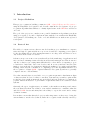
Acknowledgements
This project has enjoyed the collaboration of a great deal of people, not only in technical
aspects but supporting me emotionally during the ups and downs too. To them I am very
grateful for their time and support.
To my supervisor, Juan Climent, who has guided me during the project, helped in eventual
problems and given me advise.
To all my fellow friends and study mates that have been with me and supported me during
this project, with a particular mention to Khalid Mahyou and Daniel Martinez, whom
have accompanied me for almost the whole degree, have spent amazing moments together,
hard and good times, and have always been there to bear a hand whenever was necessary.
To my family, for their interest in my passions and patience in hard times.
4
Contents
Abstract
3
Acknowledgements
4
Table of Contents
6
1 Introduction
1.1 Project Definition . . . . . . . . .
1.2 State of Art . . . . . . . . . . . .
1.3 Project Environment . . . . . . .
1.3.1 Project Description . . . .
1.3.2 Working Tools . . . . . .
1.3.3 Working Methodology . .
1.3.4 Evaluation Methodology .
1.3.5 Possible Obstacles . . . .
1.4 Planning . . . . . . . . . . . . . .
1.4.1 Initial Planning . . . . . .
1.4.2 Changes . . . . . . . . . .
1.4.3 Final Planning . . . . . .
1.5 Costs . . . . . . . . . . . . . . . .
1.5.1 Initial Costs . . . . . . . .
1.5.2 Final Costs . . . . . . . .
1.6 Regulations and Laws . . . . . .
1.7 Social and Environmental Impact
1.8 Technical Competencies . . . . .
.
.
.
.
.
.
.
.
.
.
.
.
.
.
.
.
.
.
.
.
.
.
.
.
.
.
.
.
.
.
.
.
.
.
.
.
.
.
.
.
.
.
.
.
.
.
.
.
.
.
.
.
.
.
.
.
.
.
.
.
.
.
.
.
.
.
.
.
.
.
.
.
.
.
.
.
.
.
.
.
.
.
.
.
.
.
.
.
.
.
.
.
.
.
.
.
.
.
.
.
.
.
.
.
.
.
.
.
.
.
.
.
.
.
.
.
.
.
.
.
.
.
.
.
.
.
.
.
.
.
.
.
.
.
.
.
.
.
.
.
.
.
.
.
.
.
.
.
.
.
.
.
.
.
.
.
.
.
.
.
.
.
.
.
.
.
.
.
.
.
.
.
.
.
.
.
.
.
.
.
.
.
.
.
.
.
.
.
.
.
.
.
.
.
.
.
.
.
.
.
.
.
.
.
.
.
.
.
.
.
.
.
.
.
.
.
.
.
.
.
.
.
.
.
.
.
.
.
.
.
.
.
.
.
.
.
.
.
.
.
.
.
.
.
.
.
.
.
.
.
.
.
.
.
.
.
.
.
.
.
.
.
.
.
.
.
.
.
.
.
.
.
.
.
.
.
.
.
.
.
.
.
.
.
.
.
.
.
.
.
.
.
.
.
.
.
.
.
.
.
.
.
.
.
.
.
.
.
.
.
.
.
.
.
.
.
.
.
.
.
.
.
.
.
.
.
.
.
.
.
.
.
.
.
.
.
.
.
.
.
.
.
.
.
.
.
.
.
.
.
.
.
.
.
.
.
.
.
.
.
.
.
.
.
.
.
.
.
.
.
.
.
.
.
.
.
.
.
.
.
.
.
.
.
.
.
.
.
.
.
.
.
.
.
.
.
.
.
.
.
.
.
.
.
.
.
.
.
.
.
.
.
.
.
7
7
7
9
9
9
10
11
11
13
13
15
16
18
19
22
23
24
24
2 Sample Acquisition
2.1 Web application . . .
2.1.1 Requirements .
2.1.2 Development .
2.1.3 Hosting . . . .
2.2 Samples storage . . . .
2.3 Exporting data . . . .
2.4 Sample pre-processing
2.4.1 Completion . .
2.4.2 Resizing . . . .
2.5 Sample results . . . .
.
.
.
.
.
.
.
.
.
.
.
.
.
.
.
.
.
.
.
.
.
.
.
.
.
.
.
.
.
.
.
.
.
.
.
.
.
.
.
.
.
.
.
.
.
.
.
.
.
.
.
.
.
.
.
.
.
.
.
.
.
.
.
.
.
.
.
.
.
.
.
.
.
.
.
.
.
.
.
.
.
.
.
.
.
.
.
.
.
.
.
.
.
.
.
.
.
.
.
.
.
.
.
.
.
.
.
.
.
.
.
.
.
.
.
.
.
.
.
.
.
.
.
.
.
.
.
.
.
.
.
.
.
.
.
.
.
.
.
.
.
.
.
.
.
.
.
.
.
.
.
.
.
.
.
.
.
.
.
.
.
.
.
.
.
.
.
.
.
.
.
.
.
.
.
.
.
.
.
.
.
.
.
.
.
.
.
.
.
.
.
.
.
.
.
.
.
.
.
.
.
.
.
.
.
.
.
.
.
.
.
.
.
.
.
.
.
.
.
.
.
.
.
.
.
.
.
.
.
.
26
27
27
27
30
32
33
34
34
35
38
3 Algorithms
3.1 Gradient Histogram . . . . . . . . . . . . . . . . . . . . . . . . . . . . . .
3.1.1 Description . . . . . . . . . . . . . . . . . . . . . . . . . . . . . . .
3.1.2 Development . . . . . . . . . . . . . . . . . . . . . . . . . . . . . .
40
42
42
42
.
.
.
.
.
.
.
.
.
.
.
.
.
.
.
.
.
.
.
.
.
.
.
.
.
.
.
.
.
.
.
.
.
.
.
.
.
.
.
.
.
.
.
.
.
.
.
.
.
.
.
.
.
.
.
.
.
.
.
.
5
3.2
3.3
3.1.3 Results . . . . .
Dynamic Time Warping
3.2.1 Description . . .
3.2.2 Development . .
3.2.3 Results . . . . .
Conclusions . . . . . . .
.
.
.
.
.
.
.
.
.
.
.
.
.
.
.
.
.
.
.
.
.
.
.
.
.
.
.
.
.
.
.
.
.
.
.
.
.
.
.
.
.
.
.
.
.
.
.
.
4 Embedded System
4.1 Set-up and Configuration . . . . . . .
4.1.1 EasyPIC6 Development Board
4.1.2 Micro-controller . . . . . . . .
4.1.3 Touchpad . . . . . . . . . . . .
4.1.4 GLCD . . . . . . . . . . . . . .
4.1.5 Touchpad & GLCD - Graphical
4.2 OCR . . . . . . . . . . . . . . . . . . .
4.2.1 Data Structure . . . . . . . . .
4.2.2 Algorithm . . . . . . . . . . . .
4.2.3 Modular API . . . . . . . . . .
4.3 Overall Operation . . . . . . . . . . .
.
.
.
.
.
.
.
.
.
.
.
.
.
.
.
.
.
.
.
.
.
.
.
.
.
.
.
.
.
.
.
.
.
.
.
.
.
.
.
.
.
.
.
.
.
.
.
.
.
.
.
.
.
.
.
.
.
.
.
.
.
.
.
.
.
.
.
.
.
.
.
.
.
.
.
.
.
.
. . . . . . . . . . . . .
. . . . . . . . . . . . .
. . . . . . . . . . . . .
. . . . . . . . . . . . .
. . . . . . . . . . . . .
Liquid Crystal Display
. . . . . . . . . . . . .
. . . . . . . . . . . . .
. . . . . . . . . . . . .
. . . . . . . . . . . . .
. . . . . . . . . . . . .
.
.
.
.
.
.
.
.
.
.
.
.
.
.
.
.
.
.
.
.
.
.
.
.
.
.
.
.
.
.
.
.
.
.
.
.
.
.
.
.
.
.
. . . . . . .
. . . . . . .
. . . . . . .
. . . . . . .
. . . . . . .
- Calibration
. . . . . . .
. . . . . . .
. . . . . . .
. . . . . . .
. . . . . . .
46
48
48
49
53
56
57
57
57
60
65
66
67
70
70
70
71
73
5 Evaluation
77
5.1 Tests . . . . . . . . . . . . . . . . . . . . . . . . . . . . . . . . . . . . . . . 77
5.2 Results . . . . . . . . . . . . . . . . . . . . . . . . . . . . . . . . . . . . . . 78
5.3 Conclusions . . . . . . . . . . . . . . . . . . . . . . . . . . . . . . . . . . . 79
6 Future Work
80
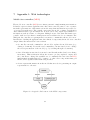
7 Appendix 1: Web technologies
81
Bibliography
83
Glossary
84
List of Figures
86
List of Tables
87
List of Codes Samples
88
6
1
1.1
Introduction
Project Definition
This project consists in building a numeric OCR - Optical Character Recognition using the EasyPIC6 development board. It will consist in the development of a proper
recognition algorithm that will have to classify digits drawn on the GLCD’s touch screen
on-board.
The goal of the project is to analyse some possible classification algorithms, test them
using prototyping tools, and to implement that with the best results in the EasyPIC6
development board making use of the on-board GLCD screen with an incorporated
touch-panel.
1.2
State of Art
The fields of computer science that are involved in this project, visualization, computer
vision and digit recognition fields are very recent because the computing power required
for the algorithms did not allow its implementation on a large scale and therefore were
only treated in the fields of research.
Advances in processors in recent years has allowed the marketing of applications and
more and more amazing features mostly in tablets and smart-phones. But it was not
only the evolution of processing units which has led to these fields of computing to grow
so much in so little time. In recent decades, and in recent years have increased the
number of research and development in efficient algorithms for recognition and machine
learning, and it was the combination of computing power and algorithms that have led
the recognition of digits (OCR - Optical Character Recognition) and more generally
computer vision to current limits.
Note that currently there is very little or no recognition systems for handwritten digits
or characters that are based on micro-controllers. Systems less powerful recognition that
we find are devices such as smart-phones and tablets, and is now that are becoming more
popular. This is an indicator of performance requirements that are necessaries for such
systems.
Currently, the types of applications you can find on the market scan images and extract
the text that is in them. In addition, some include translators to translate what the
embedded OCR detects and many have the ability to export the text found to many
document formats.
It is in this context that this whole project takes importance as they try to bring the
current limits to another level, that is, make the recognition task currently carried by
7
powerful systems, using a system much more limited. So this project is designed to
conduct a research project to evaluate different initial algorithms currently in use, and
from the digit recognizer that is developed, other students can continue and extend the
OCR.
So the project is aimed at all those who in some way or another are interested in the
field of OCR and who want to use their knowledge to bring the OCR to another world,
the world of micro-controllers.
Furthermore, this project could be the precursor of a commercial product that uses the
OCR for some specific task (such as access security, keyboard input by hand ...) and
therefore any company to take charge of product could benefit from this work as well as
anyone who wants to continue this project in case is willing to extend or improve it.
Because up to today I found no indication that this project has already been made by
someone, a priori there is no solution nor algorithm that gives the optimal solution,
and therefore must start from scratch investigating the performance of the best known
algorithms for recognition of digits to design a new solution.
8
1.3
1.3.1
Project Environment
Project Description
For the development of the project, some recognition and classification algorithms must
be tested in order to build the final OCR on the EasyPIC6 development board. These
algorithms usually require a huge amount of input data for the training phase (in which
they extract concrete features from the input data that are later used to differentiate
digits among them). So, to train the prototype algorithms that will be analysed, many
handwritten digit samples will be required. The amount of samples should be between
500 and 1000 for each digit, giving a total of 5000 to 10000 samples.
The generation and gathering o the samples will be done by developing a web application
in which users will be able to draw digits the application will ask them to draw. These
samples will be then stored in a database, and by the use of PHP scripts they will be
formatted to a suitable format to be used by the numerical calculus software Matlab.
There will be five methods of recognition and classification, being this number extendible
if some other method was found, or reducible in case any of them proved to be non-viable.
Once the algorithms are implemented they will be tested using a subset of the samples
if the algorithm’s nature requires so, or all samples otherwise. The evaluation will be
performed by calculating the confusion matrices for each algorithm, that will show the
percentages of correctly recognized and classified samples as well as those which were
classified wrong.
After algorithmic analysis, that with the best performance will be implemented in the
embedded system. In case that the implementation of the algorithm was not feasible due
to computation and memory constrains of the micro-controller the next algorithm with
best performance will be chosen, until a feasible one is found.
In case there is enough time and the remaining resources in the embedded system allow
it, the project will be extended and USB drivers will be added to the micro-controller so
that the embedded system works as a digit keyboard for a computer.
1.3.2
Working Tools
The tools that will be used during the project are very varied. Initially, for the web
application implementation the IDEs Netbeans or Eclipse will be used, both being free
and independent of the platform.
To store the data generated from the web application, a SQL database will be used,
hosted on a Linux server, and to pass the data from the database to the computer it will
be done via PHP scripts that will perform an initial formatting to allow computation on
9
the gathered data.
For the assessment of all proposed algorithms to implement an OCR, the mathematical
software Matlab will be used, since the university has licensed copies for use in FIB
classrooms, or failing that, the software Octave will be used, being the free alternative to
Matlab.
For the OCR programming on the incorporated micro-controller in the EasyPIC6 board,
the PIC18F4550, the IDE provided by the micro-controller manufacturer will be used,
the MPLABX, which is free. The programming will be done in C language and the
chosen compiler is the MPLAB XC8, which is not optimal, but it is free.
More generally, a standard PC with Windows or Linux operating system will be used,
according to the compatibility of the tools described above.
1.3.3
Working Methodology
Initially a handwritten digit sample gathering tool will be developed. Concretely, a web
application will be developed that will be hosted in a server and made public in a web
page so it may be accessible from the social networks, asking to familiars and known
people for their collaboration. The web application will ask the users to draw twenty
digits on a HTML5 canvas, that is, twice each digit.
With the gathered sample, the following classification and recognition algorithms will be
implemented using numerical calculus software Matlab.
• Gradient Histogram
• Dynamic Time Warping
• Artificial Neural Network
• K-means (removed from planning)
• Freeman codes (removed from planning)
These methods will be tested with a subset of samples reserved for validation, and a
classification will be generated based on the correctly recognized samples percentage. The
criteria to evaluate the algorithms performance may be changed during the development
of this project in case better methods were found.
Finally, the best algorithm will be implemented in a PIC micro-controller that is incorporated in the EasyPIC6 development board, using C programming language and assemble
language as well if it is necessary.
10
The method finally implemented in the micro-controller will be tested with different
digits that different people will draw on the touch screen, and the performance will
be measured by the percentage of correctly recognized samples and the average time
required for the recognition of a single digit. In case the results were not satisfactory,
the next algorithms in the classification will be implemented.
During the project, all handwritten digit samples gathered with the web application, and
those that had to be modified to meet the input requirements of the algorithms will be
included in a GIT version control repository, along with all Matlab scripts generated
with the prototyping of the recognition and classification algorithms as well as the final
C implementation of the best algorithm. The version control will be very strict, and
it will be mandatory to specify all modifications added in each change. This will allow
to keep an absolute control on the code and the generated data, and thus, know the
progression of the project in every moment.
1.3.4
Evaluation Methodology
The final project will be evaluated by testing the developed OCR. Once implemented and
operational in the development board, other people ( profiting that each person writes in
a different way) will test it the by drawing digits on the touch screen and the OCR’s
performance will be determined by the percentage of correct recognitions made and the
proximity to the correct solution in cases that fail.
Deformed digits will be tried as well in order to see how the system tolerates the noise,
or in other words, imperfections. If the resulting algorithm accepts different values for
certain variables, that is, it can be ”personalized” minimally, different settings will be
tried to maximize the percentage of correctly recognized digits and tolerance to noise.
To perform the evaluation, all digits will be tested equally, that is, analysing the same
number of tests for each digit, and the quantities will be such that the results will be
significant and allow to obtain the tendency of the OCR.
1.3.5
Possible Obstacles
The followings are possible obstacles derived from the technologies and tools used for
the development of this project. Any of them, could cause delays and changes to the
developed planning, increasing the total cost of the project.
• Servers out of service during sample acquisition phase, and so, the web application
would not be available.
• Servers out of service at any point of the project development, and therefore the
11
developed code repository is not accessible during an indeterminate period of time.
• Software that is free of charge at the beginning becomes of payment, and therefore
it would require to change to another free solution or to buy a licence.
• That the memory of the micro-controller is too small that none of the algorithms
fit.
• That the computing capabilities of the micro-controller is too limited that none of
the algorithms is feasible.
• That not enough samples are gathered for the algorithms training so the obtained
results are not as significant as expected, and thus, it leads us to the wrong
conclusion.
12
1.4
1.4.1
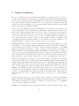
Planning
Initial Planning
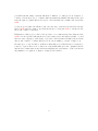
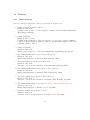
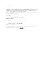
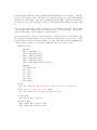
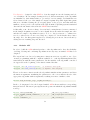
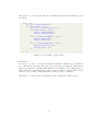
Below are described all phases of the project in chronological order.
1. Sample acquisition applet creation.
Duration: One week.
Consists on the creation of a Java applet to facilitate and automatize handwritten
digit sample gathering.
2. Sample gathering.
Duration: Three weeks.
Consists in the publication of the Java applet on a web page for anyone willing to
collaborate in the sample acquisition. Once the specified time limit is reached the
publication will be deleted.
3. Sample formatting.
Duration: One week.
Matlab script creation to convert raw samples into algorithm specific inputs.
4. Algorithm implementation (1): Gradient Histogram
Duration: One week.
Matlab implementation of Gradient Histogram algorithm.
5. Test and evaluation (1): Gradient Histogram
Duration: One week.
Test run, correction and evaluation of Gradient Histogram algorithm.
6. Algorithm implementation (2): Dynamic Time Warping
Duration: One week.
Matlab implementation of Dynamic Time Warping algorithm.
7. Test and evaluation (2): Dynamic Time Warping
Duration: One week.
Test run, correction and evaluation of Dynamic Time Warping algorithm.
8. Algorithm implementation (3): Backprop ANN - Artificial Neural Network Duration: One week.
Matlab implementation of Backprop ANN algorithm.
9. Test and evaluation (3): Backprop ANN
Duration: One week.
Test run, correction and evaluation of Backprop ANN algorithm.
13
10. Algorithm implementation (4): K-Means
Duration: One week.
Matlab implementation of K-Means algorithm.
11. Test and evaluation (4): K-Means
Duration: One week.
Test run, correction and evaluation of K-Means algorithm.
12. Algorithm implementation (5): Freeman Codes
Duration: One week.
Matlab implementation of Freeman Codes algorithm.
13. Test and evaluation (5): Freeman Codes
Duration: One week.
Test run, correction and evaluation of Freeman Codes algorithm.
14. Implementation and/or adaptation, and test of touch screen drivers.
Duration: Two weeks.
Revision, extension, adaptation and/or correction of current touch screen drivers
for EasyPIC 6 development board.
15. Implementation in C of the best algorithm.
Duration: Three weeks.
Implementation in C of the best algorithm using Microchip’s MPLABX IDE.
16. Test and evaluation on board of the best algorithm.
Duration: Two weeks.
Test run, correction and evaluation of the best algorithm on the PIC micro-controller
on the EasyPIC 6 development board.
17. Implementation and/or adaptation of USB drivers (optional).
Duration: One month.
Revision, extension, adaptation and/or correction of USB drivers for PIC microcontrollers and their installation. Make the board behave as a handwritten digit
input keyboard for PC.
18. Final degree project’s report.
Duration: One month.
To write final degree project’s report.
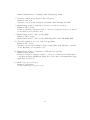
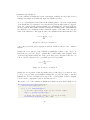
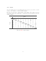
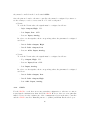
14
Figure 1: Initial planning
1.4.2
Changes
During the course of the project some phases were modified or deleted in order to fit to
the changes in the project’s requirements. All phases that have been modified or deleted
from the initial planning to the final one are listed below, as well as the reason for such
changes.
• (1) Sample acquisition applet creation.
• (8) Algorithm implementation (3): Backprop ANN
• (9) Test and evaluation (3): Backprop ANN
• (10) Algorithm implementation (4): K-Means
• (11) Test and evaluation (4): K-Means
• (12) Algorithm implementation (5): Freeman Codes
• (13) Test and evaluation (5): Freeman Codes
• (14) Implementation and/or adaptation, and test of touch screen drivers.
The first phase was modified because there was a better alternative to a Java applet
creation. It was changed by a web application developed in HTML, PHP and Javascript,
using the software pattern MVC - Model View Controller -. The reason for such
change has been a previous knowledge in the development of web applications and the
15
MVC pattern, the availability of frameworks to build user interfaces quickly and very
easily (Bootstrap, JQuery UI, etc) and the fact that PHP already has mechanisms to
communicate and perform transactions with data bases.
The six phases associated to algorithm development have been deleted because the two
associated algorithm were discarded. The reason they were discarded is because they
behave in a similar way to what Gradient Histogram does, and because of the lack of
time, I considered it was better to focus on the most important algorithms.
Both phases (1) and (14) have be enlarged to adapt to the demands that were not initially
taking into account, enlarging in two weeks the project duration.
Assuming the changes done in the initial planning, the total theoretical detour is of four
weeks, which is the total sum of the a priori stipulated time for the deleted tasks plus
the enlargement of two of them. So, the total duration of the project has been reduced.
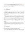
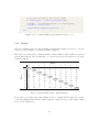
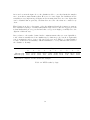
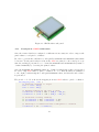
1.4.3
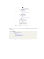
Final Planning
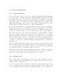
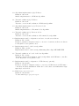
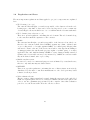
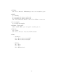
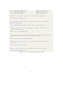
Below are described all phases of the final planning of the project in chronological order.
1. Creation of a sample acquisition web application.
Duration: Two weeks.
Consists on the creation of a Java applet to facilitate and automatize handwritten
digit sample gathering.
2. Sample gathering.
Duration: Three weeks.
Consists in the publication of the Java applet on a web page for anyone willing to
collaborate in the sample acquisition. Once the specified time limit is reached the
publication will be deleted.
3. Sample formatting.
Duration: Two weeks.
Matlab script creation to convert raw samples into algorithm specific inputs.
4. Algorithm implementation (1): Gradient Histogram
Duration: One week.
Matlab implementation of Gradient Histogram algorithm.
5. Test and evaluation (1): Gradient Histogram
Duration: One week.
Test run, correction and evaluation of Gradient Histogram algorithm.
6. Algorithm implementation (2): Dynamic Time Warping
Duration: One week.
16
Matlab implementation of Dynamic Time Warping algorithm.
7. Test and evaluation (2): Dynamic Time Warping
Duration: One week.
Test run, correction and evaluation of Dynamic Time Warping algorithm.
8. Implementation and/or adaptation, and test of touch screen drivers.
Duration: Three weeks.
Revision, extension, adaptation and/or correction of current touch screen drivers
for EasyPIC 6 development board.
9. Implementation in C of the best algorithm.
Duration: Three weeks.
Implementation in C of the best algorithm using Microchip’s MPLABX IDE.
10. Test and evaluation on board of the best algorithm.
Duration: Two weeks.
Test run, correction and evaluation of the best algorithm on the PIC micro-controller
on the EasyPIC 6 development board.
11. Implementation and/or adaptation of USB drivers (optional).
Duration: One month.
Revision, extension, adaptation and/or correction of USB drivers for PIC microcontrollers and their installation. Make the board behave as a handwritten digit
input keyboard for PC.
12. Final degree project’s report.
Duration: One month.
To write final degree project’s report.
17
Figure 2: Final planning
1.5
Costs
In the next subsections the cost of the project is discussed. For that purpose the following
costs are identified and quantified.
• Human Resources:
– Programmer
– Annalist
• Hardware:
– Web hosting
– EasyPIC6 development board
– Working computer
• Software:
– Matlab
In the context of this project, it is not economically viable. In a business context however,
assuming that there was a certain amount of money to invest in the project, then it
would be feasible, since we are talking about creating a new hardware device (software
prototype for a new person-machine interaction device (HID - Human Interface device))
that can be commercialized, and therefore profitable.
18
1.5.1
Initial Costs
In this section the initially estimated costs are analysed taking into account the initial
planning.
Note that in the corresponding cases the cost is expressed as the difference between
the product’s cost less the remaining value after applying its amortization of when the
project is over. The amortization is computed according to the BOE - Boletı́n Oficial de
Estado -[11].
The costs associated to software and hardware devices have been calculated taking
into account the current amortization rate (26%) and a amortization period (5 years)
according to the BOE [11] and using the constant amortization method as can be seen in
the calculations.
• Human Resources:
The costs associated to human resources correspond to a single person taking
different roles, assuming 5 workdays a week of 4 hours.
– Annalist:
15.625e/hour, 140 hours, tasks 5, 7, 9, 11, 13, 16
2187.5e
– Programmer:
13.020e/hour, 240 hours, tasks 1, 3, 4, 6, 8, 10, 12, 14, 15
3124.8e
• Software:
– Matlab, student version: 4.54e (Table 1)
Acquisition price
Amortization base
Monthly amortization quota
Remaining cost after the project
Cost to the project
69e (VAT included)
54.51e
0.91e
49.97e
4.54e
Table 1: Computer associated cost calculation.
• Hardware:
– EasyPIC6 development board: 7.01e. (Table 2)
– GLCD with touch panel for EasyPIC6: 1.21e. (Table 3)
19
Acquisition price
Amortization base
Monthly amortization quota
Remaining cost after the project
Cost to the project
106.42e (VAT included)
84.07e
1.4e
77.06e
7.01e
Table 2: EasyPIC6 associated cost calculation.
Acquisition price
Amortization base
Monthly amortization quota
Remaining cost after the project
Cost to the project
18.38e (VAT included)
14.52e
0.24e
13.31e
1.21e
Table 3: GLCD associated cost calculation.
– Working computer: 65.83e. (Table 4)
Acquisition price
Amortization base
Monthly amortization quota
Remaining cost after the project
Cost to the project
1000e (VAT included)
790e
13.17e
724.17e
65.83e
Table 4: Computer associated cost calculation.
– Web hosting, 4.79e/month, five months, 23.95e
– Web domain, 8.79e
TOTAL = 5423.63e
If during the implementation of the algorithms another one should be added, costs would
increase as followings for each new algorithm that would be added:
• Programmer: 13.020e/hour, 20h = 260.4e
• Analyst: 15.625e/hour, 20h = 312.5e
TOTAL = 572.9e
Similarly, if there is enough time to complete the optional task number 17, implementation
20
of USB drivers, costs would rise as follows:
• Programmer: 13.020e/hour, 120h, 1,562.4e
TOTAL = 1,562.4e
21
1.5.2
Final Costs
Taking into account the changes performed in the initial planning, the stipulated costs
vary slightly. The only changes that actually have impact in the final costs are the
deletion of the algorithms, that is, tasks eight to thirteen.
Therefore, applying the same rates previously used for the calculation of the initial costs,
the final costs would be as follows:
Increment:
• Programmer: 13.020e/hour, 40h = 520.8e
TOTAL = 520.8e
Reduction:
• Programmer: 13.020e/hour, 60h = 781.2e
• Analyst: 15.625e/hour, 60h = 937.50e
TOTAL = -1718.70e
So, after subtracting the cost of the deleted tasks, the final cost of the project would be:
5423.63e - 1718.70e + 520.8e = 4225.73e
22
1.6
Regulations and Laws
The most important regulations and laws applied to project’s components are explained
here.
• Web hosting (one.com)
The customer has all right over and is responsible of the data stored in the web
hosting space. Any kind of data can be hosted as long as it does not contain any
obvious illegal content, in which case one.com will inform the relevant authorities.
• Web domain (www.adurenator.com)
There is no special regulation conforming the web domain. The web domain belong
to the customer until the expiration of the contract.
• Github
The customer has all right over and is responsible of the data stored in github.com,
therefore the customer shall defend GitHub against any claim, demand, suit
or proceeding made or brought against GitHub by a third party alleging that
customer’s content or the use of the Service in violation of the Agreement, infringes
or misappropriates the intellectual property rights of a third party or violates
applicable law, and shall indemnify GitHub for any damages finally awarded
against, and for reasonable attorney’s fees incurred by, GitHub in connection with
any such claim, demand, suit or proceeding.
• Matlab student version
It can not be used for commercial purposes as it is limited by a student license,
therefore only students may use this software.
• MPLABX
There is no special regulations conforming the use of this software as it is freely
distributed by the micro-controllers manufacturer so the developers may build
software for their products.
• XC8 evaluation license
The free version of this version has been used during the most part of the embedded
OCR development phase. However, a 60 days evaluation license was registered in
order to use the optimizations performed by the compiler. Once this evaluation
period is over, the license will roll back to the free version.
23
1.7
Social and Environmental Impact
This project could have a significant impact in the field of human-machine interactions,
and thus may potentially have an impact on anyone who uses a laptop or desktop
computer.
For example, it may potentially inspired evolutions in current devices like conventional
keyboards that could include a digit recognition panel, or laptops’ touch panels that could
use the software developed in this project to detect more gestures/movements/forms,
among others.
In addition, it could provide a new way of user authentication, not only based on
numerical/alphanumeric access codes, but based on the writing of the users.
1.8
Technical Competencies
• CEC1.1: To design a system based on microprocessor/microcontroller.
[In depth]
Analysis and set-up of the EasyPIC6 development board for the proper interconnection of all necessary peripheral devices to the micro-controller on-board.
• CEC2.1: Analyse, evaluate, select and configure hardware platforms for the
development and execution of applications and informatics services.
[A little]
Analysis of all embedded peripheral devices available in the EasyPIC6 and configuration and set-up of those necessary for the project development.
• CEC2.2: To program considering the hardware architecture, in assembler as well
as in high level.
[In depth]
OCR programming building an API - Application Programming Interface - capable
of managing different classification algorithms, taking into account memory constraints as well as computing capabilities and communication timing requirements.
• CEC2.3: To develop and analyse software for systems based in microprocessors
and their interfaces with users and other devices.
[In depth]
Analysis and development of software for a graphical user interface for the interfacing
and management of the OCR.
• CEC2.4: Design and implement system and communications software.
24
[A little]
Analysis of the peripherals available in the microcontroller used in the project
in order to implement analog to digital conversions, timing tools and RS232 and
GLCD communications, as well as internal system configuration for its proper
functionality.
• CEC3.1: Analyse, evaluate and select the most appropriate hardware platforms
for the embedded and real time applications support.
[Sufficient]
Analysis of the feasibility of the use of the chosen micro-controller and the peripherals for the implementation of an OCR.
• CEC3.2: To develop specific processors and embedded systems; To develop and
optimize the software of these systems.
[In depth]
Implementation of an OCR previously prototyped in typical personal computer
into a 8 bit micro-controller system, taking into account not only system’s memory
and computing limitations, but its architecture (segmentation, memory hierarchy,
instruction latencies, operation latencies, etc.) and tool’s specifications (compiler,
etc.).
25
2
Sample Acquisition
In order to build an OCR, few different algorithm prototypes needed to be tested to
compare their classification effectiveness so that with best results is finally implemented
into the embedded system. These algorithms are not just static algorithms that take
some input data and transform them into the correct output, but dynamic systems that
require some previous training or pre-computation that extract features from the input
data for later use in the main algorithm.
Therefore the algorithms need data, and taking into account the project’s nature and
context, this data is concretely handwritten digit samples. But how much data is needed?
There are ten different numeric digits, from zero to nine, so in short the total amount of
data would be that that represents or incorporates all possible variants of the features to
be extracted. The aim of the project is to be able to identify handwritten digits, so for
each of the digits it is necessary to dispose a big amount of samples so different ways
of drawing and tracing them is captured. So in conclusion, about five hundred to one
thousand samples per digit would be enough for the project’s purpose.
Gathering this huge amount of data by manual introduction was definitely out of my
possibilities, so some sample gathering system was required for the task. Taking into
account that I alone would not be able to achieve it, the system had to be as multi
platform as possible and designed to reach to as many people as possible so the number of
samples available for the algorithms training was maximized. To that purpose, I hesitated
between some possible systems including a Java web applet, a web application and an
Android application. The final system would later be introduced in social networks to
make it known to related and known people so I could count with their collaboration.
The Android application would have been ideal from sample’s quality side as the users
could use the touch screen to easily draw the digits with their fingers, getting much more
realistic results than if they were drawn with a mouse. But having the smart-phones
market mainly divided between Android and iOS users, this solution limited the amount
of people the application could potentially reach. Furthermore, there was an added
difficulty of the sample’s storage. Once drawn, they would need to be safely transferred to
an external storage system like a database, and this would require an internet connection
a a way of communicating the application with an external system. This made the
Android solution become too complex for the purpose of the project, so it was definitely
rejected.
A Java web applet seemed to be a good solution since it could be done with a programming
language I already was familiar with, but like the Android solution, it required a way of
connecting an external storage system, something beyond my experience. So I definitely
opted for the web application solution.
Building a web application was a task I was already comfortable with because of my
26
previous job. I was already familiar with HTML mark-up language, PHP - Hypertext
Pre-processor - programming language and MySQL databases, so my experience made
me opt for this solution. To build the web application it has been use of the PHP[8]
online reference for a proper development.
2.1
2.1.1
Web application
Requirements
For the web application development some requirements needed to be taken into account
in order to make it easy to build, comfortable to use and to reach as many people as
possible. These requirements were critically important as the success of the application
would definitely determine the future results of the project. While a good application
may provide enough data for the later algorithmic analysis, a bad application could
gather none, making the algorithmic analysis undetermined because of the lack of enough
representative data.
Probably one of the most important aspect was the language the application was going
to build in. The language would determine the public, or in other words, the amount of
people this application could be used by. So, in order to make it as global as possible,
one could think of making it entirely in English, assuming that because of nowadays
globalization it is a language almost everybody knows. But taking into account that
the goal of the application was just to obtain handwritten digit samples, any person
whatever the age could potentially use it, so making it entirely in English would not be
such a good idea as most of the people I know and would be willing to use it are not
native English speakers. So, to maximize the amount of people could use the application,
I decided to make it multilingual, translating the original English version to Catalan and
Spanish.
Another important aspect was the programming language the application was going to
be build with. The programming languages are discussed in the following section. As to
The application structure, it was build using the HTML mark-up language as it is the
standard for web page structuring and for styling it predefined CSS styles provided by
the bootstrap framework were used.
2.1.2
Development
The development of the application started by building a welcome page to where the
users would access first, before starting to use the application itself.
In order to make the application usable a short explanation was necessary for the incoming
users to know how to use it, as well as the purpose of it. So the welcome message explains
27
that the purpose of the application is to gather handwritten digit samples to use them in
the training of prototype algorithms in my final degree project. It also asks that digits
drawn onto the drawing area are as similar as possible to how they would draw it by
hand.
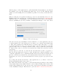
When accessing the web application main page, users are automatically redirected to the
English version of the welcome page. As stated in the previous section of requirements the
application had to be multilingual, so from the main page itself, whatever the language
users are visualizing it, gives the possibility of changing the language to any of the others.
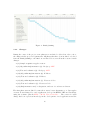
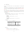
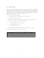
Figure 3: Web welcome page.
Once the welcome page was finished. I started with the core of the application. In order
to gather samples, two basic widgets were necessary, one to indicate users which digit
to draw, and a drawing area. But this was not enough because there had to be a way
to tell the application to move on to the next digit, or in case users did not enter the
digit properly or were not satisfied with the result, a way to restart the current digit.
To support this events, a controller area was introduced with Next and Clear buttons
respectively.
Another aspect to take into account was the fact that users would be requested to
introduce twenty digits, twice from zero to nine, and that some of them would like to stop
or quit the application before completing all, that is why a Finish button was introduced
into the controller area with the two previously mentioned buttons Clean and Next.
Furthermore, in order to give users information about the progress, a progress bar was
added.
Up to this point was the user interface of the applications core, so I had to decide how
the internal implementation was going to be.
The defined user interface was going to control the internal representation of the sample
being drawn, that is, the sample should be deleted when clicking Clear button, and
restarted when clicking Next, so the actions on the controller area would have repercussion
on the visualization widgets. That made me opt for the MVC - Model View Controller 28
Figure 4: Web drawing panel
software pattern, as it is explained in the Microsoft’s web presentation patterns page[4].
The application’s internal logic was programmed using client side JavaScript programming
language.
When users click and drag the mouse over the drawing panel, every position is notified
to the drawing controller, which asks the model to insert them to the data container
representing the sample.
When the Clear button is pressed, the associated controller orders the model to restart
the data container, and once restarted, the model notifies a status change to the implied
widgets. This way, the drawing panel can be notified and it can clear itself.
When the Next button is pressed, the associated controller asks the model to send the
introduced sample to the server. Once the transmission is over, the data container
is restarted, and the progress bar widget is notified to advance the progress, and the
drawing widget to clear itself.
When the Finish button is pressed instead, the associated controller asks the model to
finish the application, which in turn asks to the corresponding widgets and views to hide,
and to the thanking page to show itself. This behaviour is the same when the user has
finished all the samples.
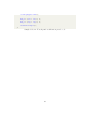
Finally, a thanking page was build. This is the page were users were redirected after the
completion of the application’s process or when users clicked on the Finish button. Like
all previous pages, this was a multilingual page too, and the language it was visualized
depended on the language selected at the welcome page.
This page thanked users for their time and collaboration and notified that the samples
had been stored safely. From this point, users could just close the page, or refresh it to
go back to the starting point.
29
Figure 5: Web drawing panel
Figure 6: Web thank you page
2.1.3
Hosting
At the beginning, in order to see development progress as well as checking and testing
the web application, it was hosted in a Raspberry Pi of my own that I transformed into a
local web server. For that purpose I installed the Nginx HTTP server, the PHP scripting
language and a MySQL database server in it.
But later, in order to make the web application accessible to anyone at any time, it had
to be hosted in a public domain. Hosting the web application in a domain was one of my
biggest concerns because depending on the application’s requirements I would need to
hire a hosting and a domain for some months.
The application’s requirements were not big at all. I did not expect many people to use
it, so assuming that I was going to publish it on Facebook the expected people would be
some of my contacts, and potentially some contacts of my contacts. This means that the
traffic would not be a problem. As for the storage requirements, the application made
use of exactly to tables, one for samples’ data storage and another one for user login
control. The amount of needed space would be determined by the number of samples
gathered, so this was an important aspect to take into account.
After a thorough search, I ended up on a one year of free hosting and domain offer at
30
One.com. Among the included services were several MySQL databases with no memory
limit and a Hosting disk space of 15GB, big enough by far for the web application.
Finally, the chose domain name was adurenator.com.
31
2.2
Samples storage
In order to store the samples gathered with the web application, a table of a MySQL
database was used. Concretely, the table stored the X and Y coordinates of the sample the
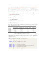
user had drawn onto the canvas, just in the very same order the sample was introduced
originally, as well as the digit the sample represented. Additionally, sample identification
number, status flag and the creation time stamp were stored.
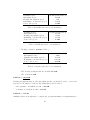
The table had the following columns:
1. id. Sample identification. There are not two equal samples.
2. digit. Digit the sample represents.
3. points. The coordinates of the sample in x,y format and sorted in arrival order.
4. checked. Integer that indicates the sample’s status.
• 0. The sample has not been checked yet.
• 1. The sample was accepted.
• 2. The sample was rejected.
5. time. A time stamp of when the sample was introduced into the database.
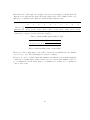
An example of a sample’s storage would be as follows:
id
1
2
3
4
digit
0
1
2
3
Table 5: Samples’ storage table example
points
checked
time
178,143;177,143;176,143;175,143;...
1
2013-11-22 18:36:38
125,189;126,188;128,186;130,185;...
1
2013-11-22 18:36:38
94,192;94,190;95,188;96,186;...
0
2013-11-22 18:36:38
90,177;90,176;91,175;92,174;...
2
2013-11-22 18:36:38
32
2.3
Exporting data
Once sample’s data was available, a way to export that data was necessary to feed the
prototype algorithms that were going to be developed using Matlab. For that purpose a
PHP script was created to transform data stored in the database into a CSV formatted
text file as it is specified in its RFC - Request for Comments - [9].
A comma-separated values (CSV) file stores tabular data (numbers and text) in plain-text
form. Plain text means that the file is a sequence of characters, with no data that has to
be interpreted instead, as binary numbers. A CSV file consists of any number of records,
separated by line breaks of some kind; each record consists of fields, separated by some
other character or string, most commonly a literal comma or tab. Usually, all records
have an identical sequence of fields.
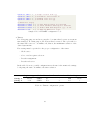
To export samples’ data to CSV formatted file, the following format was used:
• digit: A single value with the digit represented by the sample.
• coordinates: N lines with comma separated X and Y coordinates respectively.
• delimiter: an empty line representing the end of a sample data.
Table 6: Samples’ exporting CSV format example
0
178, 143
177, 143
176, 143
175, 143
174, 144
etc
1
125, 189
126, 188
128, 186
130, 185
132, 182
etc
33
2.4
Sample pre-processing
Having handwritten digits samples available was imperative for the project to continue
its course, but in order to be able to train any of the recognition algorithms proposed in
this project, a more refined data source was needed because of the HTML and JavaScript
limitations. These two technologies, as stated previously in this section, allowed to easily
build an input system to gather samples, but the raw data generated with them was in a
manner of speaking incomplete, not continuous and variable in size.
They were incomplete because JavaScript or the web browser was not fast enough to
follow peoples handwritten trace speed, so the obtained data were scarce points along
the trace’s path, just a silhouette. This same reason made raw samples not continuous
because the distance between dots was variable and depended on the trace speed. So to
higher writing speed there were less points and more separation among them, while to
lower writing speed there were more and closer.
The fact that the raw samples were variable in size was due to a design issue. The web
application had quite a wide drawing area and there was no ideal trace size indication, so
anyone who used the application could draw the digits without any size restriction but
their own will. This led two a very different range of sample sizes, to some very small,
even complicated to draw onto a screen, to huge unrealistic drawings that occupied most
of the available drawing area.
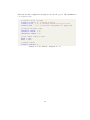
In the next two subsections are explained in detail the two main pre-processing transformations performed to raw samples to remove, correct and minimize the issues explained
above.
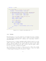
2.4.1
Completion
This transformation corrected the incompleteness and discontinuity of raw samples. To
do so the empty spaces between coordinates were removed and filled with straight lines
that interconnected two consecutive points as long as the Euclidean distance between
them was smaller than a given threshold. This threshold was necessary in order to avoid
joining two independent traces, such as for digit seven.
The process had to be applied to every pair of coordinates, for which the Euclidean
distance had to be computed in order to check whether the space between them was to
be filled or not. Then the step sizes for X and Y axis were computed, and finally, the
space between the two coordinates was filled based on the computes step sizes.
Completion ( Sample [ N ][2]) {
// Determine threshold
threshold := computeThreshold ( Sample )
34
newSample := [0][2]
for i = 0 to N -2 ,
// Insert current coordinate into new sample
newSample := insert ( newSample , Sample [ i ])
// Checking Euclidean distance is smaller than threshold
if ( euclideanDst ( Sample [ i ] , Sample [ i +1]) < threshold )
XDist := Sample [ i +1][0] - Sample [ i ][0]
YDist := Sample [ i +1][1] - Sample [ i ][1]
// Set the number of steps and step sizes
Steps := max ( XDist , YDist )
Xstep := XDist / Steps
Ystep := YDist / Steps
// Fill empty space
Xval := Sample [ i ][0]
Yval := Sample [ i ][1]
for j = 0 to Steps ,
Xval := Xval + Xstep
Yval := Yval + Ystep
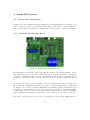
newSample := insert ( newSample , [ Xval , Yval ])
end
end
end
}
Sample Code 1: Completion algorithm pseudo-code
2.4.2
Resizing
This transformation corrected the variable size of raw samples. It is based on an image
resize algorithm that consists in mapping original coordinates (recall that raw samples
store binary bitmap (black/white) dot coordinates) to the corresponding coordinates of
the given new size.
The first step was to get sample’s maximum width and heigh because the goal of the
resizing operation was to maximize and center the sample into the given new size. With
these two values the resizing ratio was computed, that is, the biggest of the two values.
Then this ratio was used in a mere rule of three operation to map each original coordinate
into the corresponding one within the given limits.
Once the resizing done, the replicated coordinates were removed. This could potentially
happen when resizing a raw sample into a much smaller size, because some original
coordinates might end up mapped to the same new coordinate.
35
Finally, the new resized sample was centred. This was done by adding an offset (that
might be negative if the sample was drawn too much to the right or the bottom) to the
X and Y axes to make the margins correspond to the computed ideal margin that should
be to the sides of the represented bitmap.
RESIZE ( Sample [ N ][2] , XDim , YDim ) {
// Sample maximum boundary
xmax := max ( Sample [:][0])
ymax := max ( Sample [:][1])
// Sample maximum resizing ratio
ratio := max ( xmax , ymax )
// Coordinate reallocation
newSample [ n ][2]
newSample [0.. N -1][0] := round (( Sample [0.. N -1][0] * XDim ) / ratio )
newSample [0.. N -1][1] := round (( Sample [0.. N -1][1] * YDim ) / ratio )
// Remove repeated coordinates if any
newSample := removeReplicatedRows ( newSample )
N := length ( newSample )
// Centring the sample
xoffset := computeXoffset ( newSample , XDim )
yoffset := computeYoffset ( newSample , YDim )
newSample [0.. N -1][0] := newSample [0.. N -1][0] + xoffset
newSample [0.. N -1][1] := newSample [0.. N -1][1] + yoffset
}
Sample Code 2: Resizing algorithm pseudo-code
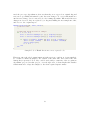
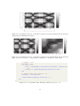
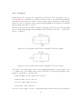
At this point a problem was detected in the resulting sample. The completion algorithm
filled all empty cells of the bitmap the sample represented in a straight line. That caused
many harsh 90o direction changes instead of smoother joins.
Figure 7: Correction of harsh directions. On the left, the result after completion. On the
right its correction.
This problem was discovered during the analysis of the prototype algorithms results
because there were tremendous amounts of horizontal and vertical directions, and that
36
made the prototype algorithms work worse than they were expected as original diagonal
traces were potentially substituted by 90o direction changes. To correct this situation a
900 direction change detector was added to the resizing algorithm. When such direction
changes are detected, they are replaced by a diagonal, making the new sample smoother,
and closer to the original aspect.
RESIZE ( Sample [ N ][2] , XDim , YDim ) {
// Resize code
...
// Removing harsh direction changes
for i = 0 to N -3 ,
dir1 := direction ( Sample [ i ][:] , Sample [ i +1][:])
dir2 := direction ( Sample [ i +1][:] , Sample [ i +2][:])
if (( dir1 == { LEFT | RIGHT } && dir2 == { UP | DOWN }) ) ||
( dir1 == { UP | DOWN }
&& dir2 == { LEFT | RIGHT })
remove Sample [ i +1]
N := N -1
end
end
}
Sample Code 3: Harsh directions corrector pseudo-code
This way, after the whole transformation (with previous completion of raw samples),
we obtained continuous samples, all of them of the same size, and centred into the
bitmap they represented. Now, they could be used safely to train any of the recognitions
algorithms proposed in this project, even though each of them might take further
transformations to adapt the samples to the their required input formats.
37
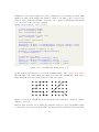
2.5
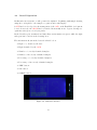
Sample results
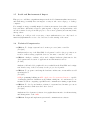
After completing raw samples, I generated users input digit’s average. To do so I
resized all samples to 30px by 30px bitmaps, and incremented by one the coordinates of
the corresponding digit that were set in each sample. Therefore, every position of the
resulting bitmaps hold the proportion (value between zero and one) of appearances for
that concrete digit.
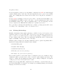
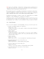
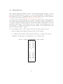
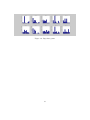
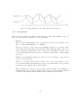
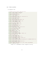
In the picture below appear the digit averages. The higher the contrast the more times
that position appeared in raw samples. As it can be seen, this picture shows how people
who used the web application tent to draw the digits.
Figure 8: Samples average
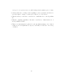
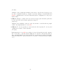
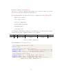
Additionally, I also generated some histogram plots showing the gradients of digits’ traces.
These histograms show sample’s curvature information, that is, how much curvature
there is for a given direction. The directions taken into account are those specified by
the Freeman Code.
Figure 9: Freeman direction code
38
Figure 10: Digit histograms
39
3
Algorithms
In this section, Matlab prototyped algorithms are discussed. As stated in the Project
Description section, part of the project’s work consists in the analysis of some algorithms
that given some samples and performed a training, are capable of recognizing new given
samples.
In the next subsections, the following algorithms are discussed:
• Gradient Histograms (GH)
• Dynamic Time Warping (DTW)
For each algorithm, its description is provided, as well as the underlying theory of why
they can be used as classification algorithms. Then, how it was developed is explained, or
if it is the case, why it could not be implemented or did not make sense to do it. Finally,
the obtained results are showed.
The following statistical information was retrieved in order to measure how well the
algorithm performed:
• Confusion matrix:
A matrix in which the rows correspond to real occurrences of the digits, and the
columns to what the classification algorithm thought it was. This representation
shows the true positives (the diagonal of the matrix) and by which digits the
classifier confused the real digit.
• Hit and miss rate by digit:
A table on which the hit and miss percentages are given for each digit. This percentages are computed over the total appearances of each digit. This representation
shows how well the classifier performs for each digit, and may help to improve it
in case digits with bad performance are detected.
• Overall hit and miss rate: A table on which the overall behaviour of the classifier
is shown. The percentage of hits and misses over all tested samples. This representation is useful to check whether certain modifications performed to the classifier
aiming to improve it actually do.
Two different classifications have been done in order to get more detailed information. In
one hand, the results are disaggregated by digits, that is, previously mentioned statistics
are given for each digit. On the other hand, the overall results are presented. This
gives a global view of how well does the algorithm perform and how easily each digit is
recognized.
By analysing the hit rates of every digit we could focus on what part of the algorithm or
40
which digit would need an improvement to optimize the obtained results. In a similar
way, by analysing the false hits, we could determine the algorithms tendency when it can
not classify a digit properly, and that information could be used to tune the algorithm to
improve the obtained results.
41
3.1
3.1.1
Gradient Histogram
Description
Gradient histogram, or commonly known as Histogram of Oriented Gradients - HOG - ,
are feature descriptors used in computer vision and image processing for the purpose of
object detection. The technique counts occurrences of gradient orientation in localized
portions of an image. For this project, the gradient orientations used are those defined
by the Freeman code.
The essential thought behind the Histogram of Oriented Gradient descriptors is that
local object appearance and shape within an image can be described by the distribution
of intensity gradients or edge directions. The implementation of these descriptors can
be achieved by dividing the image into small connected regions, called cells, and for
each cell compiling a histogram of gradient directions or edge orientations for the pixels
within the cell. The combination of these histograms then represents the descriptor. For
improved accuracy, the local histograms can be contrast-normalized by calculating a
measure of the intensity across a larger region of the image, called a block, and then
using this value to normalize all cells within the block. This normalization results in
better invariance to changes in illumination or shadowing.
Using histograms of oriented gradients have become popular in the vision literature for
representing objects and scenes. Each pixel in the image is assigned an orientation and
magnitude based on the local gradient and histograms are constructed by aggregating
the pixel responses within cells of various sizes. In this project however, the histograms
have been build from the directions obtained in the sample’s path bitmap.
For more information regarding character recognition refer to Fast and Accurate Digit
Classification[10].
3.1.2
Development
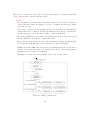
The development of this algorithm was divided in two parts. The training on the one
hand, and the validation on the other hand.
• Training:
The basic idea of the training algorithm was to obtain the gradients of all available
samples, and finally make the average grouping all partial histograms (of each
sample) by digit.
To do so, some accumulator histograms were initialized, one for each digit, and
each of them of eight bins, that it, the number of directions to take into account
according to the Freeman Chain Code. Then, each sample was resized to meet
42
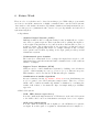
the requirements of the EasyPIC6 development board, and the histogram of this
resized sample was computed. This computed single histogram is then accumulated
to the global histogram of the corresponding digit, according to the sample.
Finally, the bins of the global histogram of each digit were divided by the total
amount of the corresponding digit, resulting in an average proportion of every
direction for each digit.
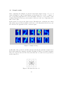
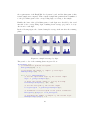
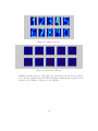
In the following figure the obtained sample’s average is shown after the training
phase.
Figure 11: Sample’s average by digit.
The pseudo-codes of the training phases is given below.
GH_Training () {
// Accumulative gradient histograms
Histograms [8][10] := 0;
// Accounting the number of samples of each digit
numSamplesDigit [10] := 0;
for i = 0 to numberOfSamples ,
// Get the represented digit by the current sample
digit := getDigit ( samples [ i ]) ;
// Reize the current sample to a 16 by 16 bitmap
resizeSample ( samples [ i ] , [16 , 16]) ;
// Get the histogram of the current sample
local_histogram := getHistogram ( samples [ i ]) ;
// Accumulate local histogram on the global accumulator
Histograms [:][ digit ] + local_histogram ;
// Increment the number of samples of the current digit
numSamplesDigit [ digit ] + 1;
43
end
for j = 0 to 10 ,
// Average histograms
Histograms [:][ i ] / numSamplesDigit [ i ];
end
}
Sample Code 4: Gradient Histogram training pseudo-code
44
• Classifier and validation:
For the validation/classification part each sample available is tested and checked
whether the sample is actually the digit the classifier decides.
To do so, each sample is resized like in the training phase to meet the requirements
of the EasyPIC6 development board, and then its gradient histogram is computed.
Next, the computed histogram is classified by calculating the similarity with the
average gradient histograms calculated during the training phase. This similarity
is computed by a cost function that returns the square of the sum of the absolute
value of the differences. The digit chosen by the classifier then is that with the lower
cost =
7
X
|Hi − hi |2
i=0
Figure 12: Chosen cost function
cost of the previously given expression, and the result is added to the confusion
matrix.
During the development of the validation/classification phase, some other cost
functions were tested in other to optimize the overall results of the classifier, most
of them being slight variations of the previously given expression and the one
bellow, but the expression above is which gave the best results.
cost =
7
X
e|Hi −hi |
i=0
Figure 13: A tested cost function
During the development of this algorithm, integer values have been used in order
to keep a proper data representation taking into account the micro-controller
limitations. In case real values were used, the overall results would be slightly
better, but the computation time would increase a lot.
The pseudo-code of the validation/classification phases is given in the figure below.
GH_Validation ( Histograms [8][10]) {
confusionMatrix [10][10] := 0;
for i = 0 to numberOfSamples ,
// Get the represented digit by the current sample
digit := getDigit ( samples [ i ]) ;
// Reize the current sample to a 16 by 16 bitmap
resizeSample ( samples [ i ] , [16 , 16]) ;
45
// Get the histogram of the current sample
local_histogram := getHistogram ( samples [ i ]) ;
costs [10] := getCosts ( Histograms , local_histogram ) ;
classifier := min ( costs ) ;
confusionMatrix [ digit ][ classifier ] + 1;
end
}
Sample Code 5: Gradient Histogram validation pseudo-code
3.1.3
Results
Once the training was done, the resulting gradient histograms were used to test the
accuracy of the classifier over all the available samples.
Digits
The table below shows the confusion matrix of this classifier. The results are given as
global values, that is, the total amount of occurrences in each case from the total of the
available samples.
a
0
1
2
3
4
5
6
7
8
9
0
1
2
3
448
6
3
0
49
7
3
2
46
17
2
441
1
0
113
0
0
2
0
50
1
1
370
18
2
28
0
75
21
1
0
0
14
361
0
56
19
1
1
1
Digits
4
5
1
36
6
0
237
6
0
64
1
46
0
2
0
46
1
315
48
1
4
15
6
7
8
9
4
0
1
61
3
29
339
1
2
46
0
5
86
2
48
23
0
345
0
0
49
0
8
7
0
4
10
2
402
9
6
10
17
8
39
24
65
3
7
307
Highlighted cells correspond to true positive matches.
Table 7: Gradient Histogram confusion matrix
As it can be seen in the table, this classifier is able to identify all the digits, but because
of the algorithms nature and the features that are extracted, some of the digit’s results
are not very satisfactory.
46
This is the case of the digit 4 for example. As every person might potentially write the
digits in a very different way than others (in a shape sense: wider, thinner, taller, etc),
this is a poor classifier if the digits are drawn in many different ways.
Digits
Hit rate (%)
Miss rate (%)
a
b
0
1
2
3
4
5
6
7
8
9
87.67
12.33
88.02
11.98
73.12
26.88
71.77
28.23
48.17
51.83
64.02
35.98
70.04
29.96
69.56
30.44
83.06
16.94
62.40
37.60
Hit and Miss rates are computed over the number of appearances of the corresponding digit.
False hits are computed over the total amount of samples.
Table 8: Gradient Histogram results by digit
Overall accuracy(%)
Hit rate
Miss rate
71.69
28.07
Table 9: Gradient Histogram overall results
However, for those digits that people tends to draw in a very similar way, the classifier
does a very good job, like with digits 0, 1 and 8 for example.
Therefore, it can be concluded that this classifier performs the best in small variability
conditions. So putting this conclusion in the project’s context, this classifier could be a
good candidate in case the input digits to be classified were restricted to be drawn in a
concrete way or size.
47
3.2
3.2.1
Dynamic Time Warping
Description
In time series analysis, dynamic time warping (DTW - Dynamic Time Warping -) is
an algorithm for measuring similarity between two temporal sequences which may vary
in time or speed. For instance, similarities in walking patterns could be detected using
DTW, even if one person was walking faster than the other, or if there were accelerations
and decelerations during the course of an observation. DTW has been applied to temporal
sequences of video, audio, and graphics data — indeed, any data which can be turned
into a linear sequence can be analysed with DTW. A well known application has been
automatic speech recognition, to cope with different speaking speeds. Other applications
include speaker recognition and online signature recognition. Also it is seen that it can
be used in partial shape matching application.
In general, DTW is a method that calculates an optimal match between two given
sequences (e.g. time series) with certain restrictions. The sequences are ”warped” nonlinearly in the time dimension to determine a measure of their similarity independent of
certain non-linear variations in the time dimension. This sequence alignment method is
often used in time series classification. Although DTW measures a distance-like quantity
between two given sequences, it doesn’t guarantee the triangle inequality to hold.
For this project, the general idea of the DTW is to compute the cost of the base gradients
sequence of each digit against sample’s gradients sequence, generating an accumulated
cost matrix with which the the optimal path is computed. Once the optimal path is
known, its cost is calculated so it is compared with the costs for the other digits, and
that with the lowest value is the result the algorithm will report.
For the development of this algorithm, it has been made use of the book Information
Retrieval for Music and Motion[7].
48
Figure 14: Time alignment of two time-dependent sequences.
3.2.2
Development
The development of this algorithm was divided in two parts. The training on the one
hand, and the classifier construction on the other hand.
• Training:
The goal of the training phase was to obtain the base sequences the classifier would
use to compare input samples to be classified.
The idea to achieve so was to have an accumulative bitmap for every digit. Then,
each sample was resized like in the Gradient Histogram algorithm to meet the
micro-controller’s requirements. Once resized, the accumulative bitmap of the
corresponding digit was incremented by one in the positions where resized sample
was active.
Finally, each accumulative bitmap was divided by the total number of appearances
of the corresponding digit.
All these operations resulted in a set (eight, one for every digit) matrices, where
every position’s value represents the proportion, or how much that concrete position
was active in the samples. The result was this:
These bitmaps were then used along with a visual analysis of the samples to
manually refine a set of sequences made from the most popular or the most likely
positions in the bitmaps. The resulting refined bitmaps looked like this:
49
Figure 15: Sample’s average.
Figure 16: Generated bitmaps.
Finally, the time-series for each digit were generated from the Freeman Chain
Code direction definitions and the refined bitmaps, resulting in the sequences below
that were the definitive sequences for the classifier.
50
Figure 17: Resulting sequences.
• Classifier and validation:
During this phase, each sample is treated independently. For every available
sample, first a resize is performed to meet the micro-controller’s requirements, and
its Freeman sequence is computed from its coordinates. Then, for each digit, the
accumulated cost matrix is computed of the corresponding digit over the sample’s
computed sequence1 .
Finally, the path with the minimum cost is calculated for every computed accumulated matrix, and that with the smallest cost is chosen by the classifier. Then the
result is added to the confusion matrix.
The figures below show a cost matrix and an accumulated cost matrix examples
with the minimum cost warped path marked on them.
\ gls { DTW } _ V a l i d a t i o n _ C l a s s i f i c a t i o n ( Sequences [10]) {
confusionMatrix [10][10] := 0;
for i = 0 to numberOfSamples ,
// Get the represented digit by the current sample
digit := getDigit ( samples [ i ]) ;
// Reize the current sample to a 16 by 16 bitmap
resizeSample ( samples [ i ] , [16 , 16]) ;
// Compute sample ’s Freeman sequence
sequence := \ gls { DTW } _Sequence ( samples [ i ]) ;
1
For more information about the algorithm and how all calculations are done, refer to the projects
code and to the provided bibliography.
51
Figure 18: Cost matrix of the two real-valued sequences X (vertical axis) and Y (horizontal
axis) using the Manhattan distance.
Figure 19: Cost matrix of the two real-valued sequences X (vertical axis) and Y (horizontal
axis) on the left, and the corresponding accumulated cost matrix on the right.
// Compute costs
costs [10] := 0;
for j = 0 to 10 ,
costM := \ gls { DTW } _AccumCostMatrix ( sequence , Sequences [ i
]) ;
costs [ i ] := \ gls { DTW } _MinWarpedPathCost ( costM ) ;
end
// Select digit with smallest cost
classifier := min ( costs ) ;
confusionMatrix [ digit ][ classifier ] + 1;
end
}
Sample Code 6: Dynamic Time Warping validation pseudo-code
52
3.2.3
Results
Once the training was done, the resulting time-series (sequences) were used to test the
accuracy of the classifier over all the available samples.
Digits
The table below shows the confusion matrix of this classifier. The results are given as
global values, that is, the total amount of occurrences in each case from the total of the
available samples.
a
0
1
2
3
4
5
6
7
8
9
0
1
2
3
198
1
1
0
98
8
68
1
17
9
1
426
3
7
32
0
0
5
2
3
17
22
346
4
8
4
1
29
18
9
0
1
7
481
0
69
0
0
51
3
Digits
4
5
3
5
0
3
263
10
3
2
0
1
28
0
0
1
3
192
92
0
49
99
6
7
8
9
144
0
0
0
0
89
201
0
12
20
5
46
146
7
0
4
3
459
13
12
0
0
1
0
0
7
0
0
292
2
115
0
2
0
88
109
116
0
30
334
Highlighted cells correspond to true positive matches.
Table 10: DTW confusion matrix
53
As it can be seen in the figure above, the classifier is able to correctly identify the samples
more often that it miss-classifies them. However, for some digits, the classification rate
variability is very high among all digits, in the meaning that there are some digits that
can be classified almost perfectly, but that there are some other that are confused very
often.
This behaviour is due to the nature of the algorithm itself and the features it extracts.
The classifier is trying to identify handwritten digit’s traces, and the biggest problem
is that handwriting is very personal and that every person might potentially trace the
digits in a different way.
In accordance to the results obtained in the confusion matrix, there are some digits like 1,
3 and 7 that are usually traced in a similar way by different people, but those digits with
a more asymmetric aspect or more elaborated traces are more likely to be miss-classified
because of their trace’s variability, which is translated to a very different time-series for
the classifier to identify.
Digits
Hit rate (%)
Miss rate (%)
a
b
0
1
2
3
4
5
6
7
8
9
38.75
61.25
85.03
14.97
68.38
31.62
95.63
4.37
53.46
46.54
39.02
60.98
41.53
58.47
92.54
7.46
60.33
39.67
67.89
32.11
Hit and Miss rates are computed over the number of appearances of the corresponding digit.
False hits are computed over the total amount of samples.
Table 11: DTW results by digit
54
Therefore, taking into account the results obtained, it can be concluded that this classifier
performs well in a little variability environment in terms of digit tracing, meaning that if
the input samples are drawn in the way the algorithm expects, then it is very likely that
the classifier will identify the sample correctly.
Overall accuracy (%)
Hit rate
Miss rate
64.19
35.57
Table 12: DTW overall results
55
3.3
Conclusions
As it has been concluded in the conclusions section of each tested algorithm, they both
perform properly as long as the input samples to be identified meet the requirements or
are similar to what the algorithms know how to classify.
Both algorithms extract or analyse different kind of features to which the inputs must
be adapted in order to be identified correctly. The Gradient Histogram analyses the
directionality of the input samples, so as long as they come in the average computed
in the training phase, it is likely they will be identified. A similar think happens with
the Dynamic Time Warping algorithm. In this case the algorithms focus in how the
input samples are traced in time, therefore if they are drawn following a similar trace
the algorithm knows then it is vary likely they will be identified correctly too.
This means that both algorithm perform well detecting the features they are supposed to
find, but the biggest problem at this point is that handwritten digits con not be identified
perfectly by just analysing single or standalone features, but a set of them might be
required for a proper classifier. Therefore, the top conclusion regarding algorithmic
analysis is that to build a complete OCR with guarantees for success, several single
feature classifiers should be combined to build a more complex system.
Taking into account that the goal of the project is to use the EasyPIC6 development
board as an OCR and not to build the ultimate classifier, the Gradient Histogram
algorithm has been chosen to be implemented on it. The reason of this selection is not
only the overall results obtained by the classifier (that were better than in the Dynamic
Time Warping), but also the simplicity of the algorithm itself. While the complexity of
Gradient Histogram is linear, the complexity of Dynamic Time Warping is quadratic, and
that makes it a poorer candidate taking into account the limited memory and computing
capabilities of the system in which the OCR will be build.
56
4
Embedded System
4.1
Set-up and Configuration
In this section all configurations and settings used in the EasyPIC6 development board
will be discussed so the project working context may be reproduced by anyone willing to,
from board’s jumper and switches configuration to the used micro-controller’s settings.
4.1.1
EasyPIC6 Development Board
Figure 20: EasyPIC6 Development board
The EasyPIC6 development board comes with an extensive set of functionalities, devices
and expansion ports, so in order to build the project on such a versatile environment
a concrete configuration has been set. In this section all relevant configurations are
discussed, as well as the micro-controller used and how the chosen configuration affects
it.
As stated before, the board comes with a set of devices that are necessary for the project,
like the RS-232 communication transceiver, buttons, GLCD display and its touch panel
for instance, as it can be seen in the EasyPIC6 user manual[6] and the EasyPIC6 board
schematics[5] in which this section is based. As this board binds several functionalities
to single pins, we need to choose the appropriate settings in the provided mechanisms,
such as jumpers and switches to ensure the correct connection to the micro-controller.
The micro-controller used on the board to program the prototyped algorithm with best
57
results and drive all the necessary peripherals is the PIC18F4550, an 8 bit micro-controller.
For the development of the embedded code, it has been made use of the PIC18F4550
data sheet[3] for the micro-controller programming, and the XC8 compiler user manual[2]
for the proper use of the available resources as well as the build-in functions included in
it.
Below are the settings used on the development board, classified by module. The settings
corresponding the to jumpers are given as Jx and those corresponding to switches are
given as SWx where x is the jumper or switch number.
For the jumpers the connected option is specified or N/A in case it does not matter. For
the switches, an hexadecimal code is given instead. All switches on-board are of eight
positions, therefore the given hexadecimal code is two digit long, the most significant bit
corresponding to position one and least significant bit to the position eight.
• External ports:
– Switches:
SW1 = 0x04
SW2 = 0x00
SW3 = 0x00
SW4 = 0x00
SW5 = 0x00
SW6 = 0x01
RA5 on.
All disabled.
All disabled.
All disabled.
All disabled.
LCD-GLCD backlight on.
– Jumpers:
J1 = Pull Down.
J2 = N/A.
J3 = N/A.
J4 = N/A.
J5 = N/A.
J18 = N/A.
J19 = N/A.
• PS/2:
J20 = Not connected. PS/2 signals not assigned to micro-controller pins.
• ADC - Anagol to Digital Converter - Input:
J15 = Not connected. ADC input not assigned to pins.
• USB Comm:
J12 = I/O all three connectors.
• RS232 Comm:
SW7 = 0x80. RX assigned to RC7.
SW8 = 0x80. TX assigned to RC6.
58
• DSI820:
J11 = Not connected. DS1820 temp. sensor not assigned to pins.
• ICSP:
J7 = MCLR.
J8 = 1st and 3rd connectors selected.
J9 = 1st and 3rd connectors selected.
J10 = The pins in the middle connected for all three connectors.
• Power Supply:
J6 = USB power supply.
• LEDs & Touch panel:
SW9 = 0x0F. LEDs off, touch-panel controller pins on.
• Buttons:
J17 = VCC.
J24 = Not connected. Protection NOT disabled.
• Misc:
– Oscillators:
J13 = Both connectors as OSC.
J14 = Both connectors as I/O.
– IO Pins:
J16 = N/A.
J23 = N/A.
J22 = RA0 selected.
59
4.1.2
Micro-controller
• Configuration bits:
// System Clock Postscaler Selection bits
# pragma config CPUDIV = OSC1_PLL2
// PLL Prescaler Selection bits
# pragma config PLLDIV = 2
// USB Clock Selection bit
# pragma config USBDIV = 2
// Internal / External Oscillator Switchover bit
# pragma config IESO = OFF
// Oscillator Selection bits
# pragma config FOSC = HS
// Fail - Safe Clock Monitor Enable bit
# pragma config FCMEN = OFF
// USB Voltage Regulator Enable bit
# pragma config VREGEN = OFF
// Brown - out Reset Enable bits
# pragma config BOR = ON
// Brown - out Reset Voltage bits
# pragma config BORV = 1
// Power - up Timer Enable bit
# pragma config PWRT = ON
// Watchdog Timer Postscale Select bits
# pragma config WDTPS = 32768
// Watchdog Timer Enable bit
# pragma config WDT = OFF
// CCP2 MUX bit
# pragma config CCP2MX = OFF
// PORTB A / D Enable bit
# pragma config PBADEN = OFF
// Low - Power Timer 1 Oscillator Enable bit
# pragma config LPT1OSC = OFF
// MCLR Pin Enable bit
# pragma config MCLRE = ON
// Background Debugger Enable bit
# pragma config DEBUG = OFF
// Stack Full / Underflow Reset Enable bit
# pragma config STVREN = OFF
// Dedicated In - Circuit Debug / Programming Port ( ICPORT ) Enable bit
# pragma config ICPRT = OFF
// Extended Instruction Set Enable bit
# pragma config XINST = OFF
// Single - Supply ICSP Enable bit ( low voltage programming )
# pragma config LVP = OFF
Sample Code 7: PIC18F4550 relevant configuration bits setup.
60
• Analog to digital converter (ADC):
In order to be able to read the position where the touch-screen has been pressed,
the ADC module has configured for that purpose.
Few settings must be specified for the proper configuration of the ADC module.
– High voltage reference.
– Low voltage reference.
– A/D port configuration.
– Result justification format.
– Acquisition time.
– Conversion clock.
Following the PIC18F4550 data-sheet and taking into account module’s requirements, the following configurations have been concluded.
Vref+
Vref-
A/D Port
Result justification
Acquisition time
Clock
VDD
VSS
AN0 & AN1
right
4 TAD
FOSC / 8
Table 13: ADC configuration
The initialization code is given below.
// Set channels AN0 and AN1 as inputs
TRISA |= 0 x03 ;
// Set analog pins
ADCON1bits . VCFG1 =
ADCON1bits . VCFG0 =
ADCON1bits . PCFG =
// Set sampling
ADCON2bits . ADFM
ADCON2bits . ACQT
ADCON2bits . ADCS
and voltage references
0;
// Voltage Reference Configuration as VSS
0;
// Voltage Reference Configuration as VDD
0 b1101 ; // Set AN0 and AN1 channels
timing configs
= 1;
// ADC Result right justified
= 0 b111 ; // 4 TAD adquisition time
= 0 b001 ; // FOSC /8 \ gls { ADC } Conversion Clock
Sample Code 8: ADC configuration code
61
• Asynchronous Serial Transceiver (EUSART - Enhanced Universal Synchronous
Asynchronous Receiver Transmitter -):
For debugging purposes and as communication tool, the USART module has
been configured to communicate with a host computer using the RS-232 serial
communication protocol.
Few setting must be specified for the proper configuration of the USART module.
– EUSART mode selection.
– Baud rate speed mode selection.
– Baud rate.
– 9/8 bit transmission.
– 8/16 bit Baud Rate register selection.
– Error monitoring.
In the table below, four possible configurations are shown for the mentioned settings
and for a 9600 baud rate target.
Config.
Config.
Config.
Config.
Speed mode
Register type
Register value
Error(%)
Low
Low
High
High
8 bit
16 bit
8 bit
16 bit
13
52
52
208
0.15
0.15
0.15
0.15
1
2
3
4
Table 14: EUSART configuration options
Currently the first configuration settings are used in the project. The initialization
code is given below.
SPBRG
= ( unsigned char ) (12) ; // 9600 bits / sec
// Set Tx and Rx pins
TRISCbits . RC6 = 0; // TX pin set as output
TRISCbits . RC7 = 1; // RX pin set as input
// Set EUSART config
TXSTAbits . TX9 = 0; //
TXSTAbits . SYNC = 0; //
TXSTAbits . BRGH = 0; //
TXSTAbits . TXEN = 1; //
RCSTAbits . RX9
8 bit transmission
Asynchronous mode
High Baud Rate Select bit ( low speed )
Transmission enable
= 0; // 8 bit reception
62
RCSTAbits . SREN
RCSTAbits . CREN
RCSTAbits . FERR
RCSTAbits . OERR
=
=
=
=
0;
1;
0;
0;
//
//
//
//
Single receive mode off
Continuous receive mode on
Framing error bit off
Overrun error bit off
// Baud rate config
BAUDCONbits . RXDTP =
BAUDCONbits . TXCKP =
BAUDCONbits . BRG16 =
BAUDCONbits . WUE
=
0;
0;
0;
0;
//
//
//
//
Recv Data Polarity not inverted
Clock and Data Polarity not inverted
16 - Bit Baud Rate Register off - 8 bit
Wake - up Enable bit ( off )
Sample Code 9: EUSART configuration code
• Timers:
For debugging purposes and as a general tool, a timer has been set as a system
time manager. For that purpose the Timer0 has been used. The cycle time for
the timer has been set to one millisecond, that is, the maximum resolution of the
desired system time.
Few setting must be specified for the proper configuration of the timer.
– Clock source.
– 8 bit or 16 bit register selection.
– Prescaler assignment.
– Prescaler selection.
In the table below two possible configurations are shown for the mentioned settings,
both giving the same one millisecond time resolution.
Config. 1
Config. 2
a
Register type
Clock
Prescaler
Prescaler value
Ticks
Register value
16 bit
8 bit
CLKO
CLKO
No
Yes
8
2000
255
63535
5
CLKO: Internal instruction cycle clock. CLKO = FOSC /4
Table 15: Timer0 configuration options
63
Currently the first configuration settings are used in the project. The initialization
code is given below.
// Timer0 control settings
T0CONbits . T08BIT = 0; // 16 - Bit register
T0CONbits . T0CS
= 0; // Internal instruction cycle clock
T0CONbits . PSA
= 1; // Prescaler Assignment bit ( bypassed )
// Timer0 interrupt flags
INTCONbits . TMR0IF = 0;
INTCONbits . TMR0IE = 1;
INTCON2bits . TMR0IP = 1;
// Set timer0 register value
TMR0H = 0 xF8 ;
TMR0L = 0 x2F ;
// Enable timer0
T0CONbits . TMR0ON = 1;
Sample Code 10: Timer0 configuration code
64
4.1.3
Touchpad
In this subsection touch-panel’s configuration is discussed. The touch-panel of the onboard’s GLCD is of resistive type, that is, it has two layers of a resistive material that
when they are in contact, the position of the pressure can be calculated from the analog
values. For the development of the touch-panel and GLCD drivers and its user manual
and specifications[1] have been used.
These two layers are used as tension dividers depending on how the sources and the sinks
are set. In the following figures the resulting tension dividers are shown to obtain the X
and Y coordinates.
Figure 21: Touch panel tension divider diagram for X value reading.
Figure 22: Touch panel tension divider diagram for Y value reading.
As it can be seen in the figures, there are four signals that must be set properly in order
to configure the corresponding tension divider. The list below shows the mapping of the
signals to actual micro-controller pins.
• DriveA: RC0. (Control Right, Top and Left).
• DriveB: RC1. (Control Bottom).
• Bottom: RA0 - AN0. (Read X).
• Left: RA1 - AN1. (Read Y).
In order to use the pins to set the corresponding tension divider and read the touch-panel
65
they must be enabled in the board’s switch SW9.
Once the pins are bound to the micro-controller, they must be configured by software to
set the circuity to read a concrete axis X or Y of the touch-panel.
• X axis:
To read the X axis value, the signals must be configured as follows:
– Right: Output, High. Vdd.
– Left: Input, Low. GND.
– Bottom: Input, Analog.
In order to set the signals to their corresponding values, the pins must be configured
as follows:
– DriveA: RC0. Output, High.
– DriveB: RC1. Output, Low
– Bottom: AN0. Input, Analog.
• Y axis:
To read the Y axis value, the signals must be configured as follows:
– Top: Output, High. Vdd.
– Bottom: Input, Low. GND.
– Left: Input, Analog.
In order to set the signals to their corresponding values, the pins must be configured
as follows:
– DriveA: RC0. Output, Low.
– DriveB: RC1. Output, High
– Left: AN1. Input, Analog.
4.1.4
GLCD
For the GLCD to work, there is not any particular configuration to take into account, it
is just digital communication what drives the GLCD. However, there are some pins that
must be reserved for the exclusive use of the communication between the micro-controller
and the GLCD controller: Port B, pins 0 to 5 (RB0:5) and Port D, the whole port.
66
Figure 23: GLCD with touch panel
4.1.5
Touchpad & GLCD Calibration
Once the tension divider is configured, a calibration is necessary in order to map touchpanel values to real pixel coordinates.
In order to perform the calibration, touch-panel’s maximum and minimum values must
be known. Touch-panel values read from the ADC are printed to the serial port every
time the reading is performed, so to obtain the minimum and maximums they must be
obtained manually by observing the printed values.
Once the maximum and minimum values are obtained, a simple rule-of-three is performed
in order to map ADC values to pixel coordinates. To do so, first all values are translated
to the origin by subtracting the touch-panel minimum values, and then the rule-of-three
is performed.
The pseudo-code below shows the mapping from raw ADC values to pixel coordinates.
PixelMapping ( valX , valY ) {
// Translate readings to origin
valX := valX - MIN_X ;
valY := valY - MIN_Y ;
// Readings mapping by the rule of three
coordinateX := ( valX * 128) / ( MAX_X - MIN_X ) ;
coordinateY := ( valY * 64) / ( MAX_Y - MIN_Y ) ;
// Coordinate security checking
if ( coordinateX > 127) coordinateX := 127;
if ( coordinateY > 63) coordinateY := 63;
// Inverting Y coordinate because touch - panel is inverted
coordinateY := 63 - coordinateY ;
67
}
Sample Code 11: ADC reading to pixel coordinate mapping pseudo-code
These values obtained from observation will be used by default every time the development
board is restarted, but an online calibration system have been added to the project to
re-calibrate the touch-panel values in case changes in environmental conditions affect
the readings.
For that purpose a different system has been set that works apart from the normal
operation mode but that is embedded in it. When the calibration mode is accessed (by
long pressing the RA5 button) the user has to press on the dots shown in the GLCD
(each corner of the GLCD), and the system records the new maximum and minimum
values computed from the readings. For later ADC value to pixel coordinate mappings
the newly computed calibration values are used.
For this calibration system to work, interrupts are disable when the calibration mode is
accessed so it is done isolated from the system and the normal execution mode. Once the
calibration is finished (the user has pressed on all four corners and the new minimum
and maximum values have been computed), interrupts are re-enabled and the execution
gets back to the normal operation mode.
The pseudo-code below shows how the calibration system is build.
Calibration () {
disableInterrupts () ;
// Top left corner
drawTopLeftCorner () ;
while (! touchPanelIsPressed () ) ;
[ tlx , tly ] = readTouchPanel () ;
clearTopLeftcorner () ;
// Lower left corner
drawLowerLeftCorner () ;
while (! touchPanelIsPressed () ) ;
[ llx , lly ] = readTouchPanel () ;
clearLowerLeftCorner () ;
// Lower right corner
drawLowerRightCorner () ;
while (! touchPanelIsPressed () ) ;
[ lrx , lry ] = readTouchPanel () ;
cle arLo werR ightC orne r () ;
// Top right corner
drawTopRightCorner () ;
while (! touchPanelIsPressed () ) ;
[ trx , try ] = readTouchPanel () ;
68
clearTopRightCorner () ;
MIN_X
MAX_X
MIN_Y
MAX_Y
=
=
=
=
( tlx
( trx
( lly
( tly
+
+
+
+
llx )
lrx )
lry )
try )
/
/
/
/
2;
2;
2;
2;
enableInterrupts () ;
}
Sample Code 12: Touch-panel recalibration pseudo-code
69
4.2
OCR
As commented in the conclusions of the algorithms analysis section the Gradient Histogram algorithm has been implemented on the EasyPIC6 development board.
In this subsection the software side of the Gradient Histogram is explained. The data
representation and how it has been structured in the system’s software is explained on
the one hand, and how the algorithm works on the other hand, as well as the designed
API to handle various algorithms in a easy way.
4.2.1
Data Structure
In order to implement the Gradient Histogram algorithm some data structures are
necessary.
• Histogram
The base data structure in which every direction will be counted. Having eight
different directions according to the Freeman Chain Code this structure will be an
8 element array.
• Base histograms
Average histograms of each digit obtained during the training phase when testing
the prototype algorithm. These are the histograms against which the sample will
be compared.
• Costs
A data structure containing the cost function value of each base digit against the
sample being recognised. The digit the OCR will report will be that with the lowest
value in this structure.
4.2.2
Algorithm
In order to implement the Gradient Histogram in the micro-controller a polling system
has been set up which is repetitively checking whether the touch panel is pressed. If
it is, the coordinates are passed to the algorithm which computes the direction against
the previous coordinate and builds the current sample’s histogram using eight different
type of directions that correspond to the Freeman Chain Code. Therefore, it is an
on-the-fly calculation, meaning that partial calculations are performed upon reception of
new coordinates instead of waiting to have the whole sample, saving memory space in
the micro-controller and making the whole system more responsive.
Once the sample is complete, the user may notify the system using a GUI - Graphical
70
User Interface - designed for the GLCD to clear the sample in case the drawing was bad,
or to identify it. In case sample clearing is selected, all data structures of the algorithm
are initialized to their initial values to get ready for a new sample. If identification is
selected instead, the cost of the sample is computed against all possible digit’s histograms
that were calculated during the prototyping phase of the project, and that with the
smallest cost is reported to the system as the digit identified, updating system’s statistical
data and the information shown in the GLCD’s user interface.
Additionally, a 90o direction change detection has been implemented as was commented
in the Sample Acquisition section to remove harsh directions, make the sample smoother
and therefore improve algorithm’s accuracy. To do so, the previous two coordinates are
stored, so when a new one is received they are compared to check whether they form a
90o angle. If so, the histogram is updated by deleting the previous two directions and by
adding the new resulting diagonal direction.
4.2.3
Modular API
In order to build the OCR with independence of the algorithm and to have the flexibility
of adding, deleting and combining algorithms in an easy way, an unified API has been
designed.
The way it has been done is by using macro functions as it is not possible to use object
oriented programming with the compilers available. So, each algorithm implements the
same functions with the same parameters, but the initials of the algorithm or method
are appended at the beginning of the function name like this:
unsigned char GH_Classify ( void ) ; // Gradient Histogram
unsigned char DTW_Classify ( void ) ; // Dynamic Time Warping
Therefore the macro functions take the algorithm’s initials as first parameter and then
the function arguments, translating the parameters to the correct function header of the
appropriate algorithm with its arguments, resulting in a macro similar to this:
# define OCR_Classify ( _alg ) _alg ## _Classify () ;
In the code fragment below, the designed unified API is shown with its corresponding
function headers. The interrogate sign shows the position in which the algorithm’s initials
would go.
# define INIT_ALGORITHM ( _a )
# define SA MP LE_ UP DA TE _CA LL BA CK ( _a , _b , _c )
) , ( _c ) )
# define CLASSIFY ( _a )
71
_a ## _init_algorithm ()
_a ## _samp leUp dateC allb ack (( _b
_a ## _classify ()
# define GET_LAST_CLASSIFIED ( _a )
# define GET_COST_VALUES ( _a )
# define SAMPLE_DISCARD ( _a )
_a ## _getLastClassified () ;
_a ## _getCostValues () ;
_a ## _sampleDiscard () ;
/*
* Initializes the data structures required by the algorithm .
*/
void ? _init_algorithm ( void ) ;
/*
* Notification function called every time a pressure is detected
* on the touch panel .
*/
void ? _s ampl eUpda teCa llba ck ( unsigned char x , unsigned char y ) ;
/*
* Function that uses the data gathered to predict which digit the
* sample corresponds to .
*/
unsigned char ? _classify ( void ) ;
/*
* Function that returns the last prediction of the algorithm without
* executing the whole classification algorithm again .
*/
unsigned char ? _getLastClassified ( void ) ;
/*
* Function that returns the costs associated of the sample against
* each digit .
*/
float * ? _getCostValues ( void ) ;
/*
* Resets or initializes the data structures of the algorithm .
*/
void ? _sampleDiscard ( void ) ;
Sample Code 13: OCR algorithm managing API
72
4.3
Overall Operation
In this subsection system’s overall operation is explained. Beginning with sample drawing
using the touch-panel to the sample recognition and result display.
A GUI has been developed for the management of the OCR on the EasyPIC6 development
board. Concretely, the GLCD has been divided horizontally in two regions, leaving two
equal size subregions of 64 by 64 pixels.
In the left subregion, statistical and miscellaneous information is given, while the right
subregion has been left as the drawing area.
The information shown in the left side is listed below:
• Digit to be drawn by the user.
• Digit identified by the OCR.
• Number of correctly identified samples.
• Number of incorrectly identified samples.
• Percentage of correctly identified samples.
• Percentage of incorrectly identified samples.
• NEW button.
• GO button.
• CLEAR button.
Figure 24: OCR user interface
73
There are two operation modes, both accessed from the main loop of the program. The
OCR operation mode, and the calibration mode.
• OCR:
In every main loop iteration the touch-panel values are read, and if a pressure is
detected then the values are mapped to proper coordinates and checked to which
region they belong.
In case they correspond to the drawing area the GUI is updated by activating the
pixels in the new coordinates, and the algorithm layer is notified to add them to
its data structures or perform the necessary operations with them.
In case the CLEAR button is pressed, the drawing area in the GUI is cleared, and
the algorithm layer is notified to discard all its data.
In case the GO button is pressed, the OCR identifies the sample drawing and the
GUI is updated with the digit reported and the re-computed statistics.
Finally, in case the NEW button is pressed, the drawing area in the GUI is cleared
and the OCR changes the digit to be drawn by the user so the following sample
identifications are compared to this digit.
The figure below shows the flow diagram of the OCR operation mode.
Figure 25: OCR operation mode
74
The pseudo-code below shows the on-board implementation of the interrupt operation mode.
while (1) {
[x , y ] = readTouchPanel () ;
if ( isPressed (x , y ) ) {
[ x1 , y1 ] = getCoordinates (x , y ) ;
if ( isButtonGo ( x1 , y1 ) ) {
digit = OCR_Identify () ;
GLCD_Recognized ( digit ) ;
}
else if ( isButtonCLEAR ( x1 , y1 ) ) {
GLCD_ClearDrawing () ;
OCR_DiscardData () ;
}
else if ( isDrawingArea ( x1 , y1 ) ) {
GLCD_DrawPoint ( x1 , y1 ) ;
OCR_Notify ( x1 , y1 ) ;
}
}
}
Sample Code 14: OCR operation mode
• Calibration:
In order to be able to perform on-the-fly touch-panel calibration, a calibration
procedure has been set-up. The way to access it is by pressing the RA5 button
and keep it pressed for a little while until the GUI changes to the calibration mode.
Then, the active pixels must be pressed so the system records its values and is
therefore able to map touch-panel analog values to pixel coordinates.
The figure below shows the flow diagram of the calibration operation mode.
75
Figure 26: Calibration operation mode
The pseudo-code below shows the on-board implementation of the calibration
operation mode.
while (1) {
if ( RA5 ) {
_delay ( accessDelay ) ;
if ( RA5 ) {
InterruptsDisable () ;
Calibrate () ;
InterruptsEnable () ;
}
}
}
Sample Code 15: Calibration operation mode
76
5
Evaluation
In this section the OCR’s evaluation is explained, how it has been done and what the
results obtained are. Finally, the conclusions are given taking into account the results.
5.1
Tests
In order to test the OCR the following tests have been made in the way the digits are
drawn on the GLCD.
Two types of tests have been differentiated, those that have been done drawing standard
traces and those with disfigured traces. Standard traces means those that are typically
shown in informatics systems as standard digit visualizations, and disfigured traces means
those more personal ways of drawing digits (person dependant) and those with slightly
disfigured areas to test the noise resistance.
For both type of tests, the following tests have been performed, and for all tests, it
has been assumed that the size of the drawing will remain unchanged to reduce results
variability.
• Constant trace speed
The drawing have been made keeping a constant speed, resulting in a constant
proportion of data (number of directions read) per traced distance.
– Slow trace speed
The drawing have been made keeping a low constant speed, resulting in a
constant proportion of data, but gathering more data than in the previous test
due to the lower speed. The lower the speed, the more data will the system
be able to read, and therefore the more precise the results should be.
– Fast trace speed
The drawing have been made keeping a higher constant speed, resulting in
a constant proportion of data, but gathering less data than in any previous
test. The higher the speed, the less data will the system be able to read, and
therefore the less precise the results should be.
• Variable trace speed
The drawing have been made varying the trace speed in certain arbitrary zones of
the drawing. This should theoretically lead the algorithm to an incorrect proportion
of data, resulting in wrong recognitions.
77
5.2
Results
• Standard traces:
For constant speed tests, the results vary depending on the trace speed.
For low speed traces, there was far more data available for the algorithm to perform
the recognition. This could be seen by checking the drawing area, as the speed was
lower, there were more pixels active in trace’s path. However, instead of leading
the algorithm to more accurate results, it misclassified several digits because of the
extreme concentration of data around trace’s path (there might be several different
readings for the same position), adding a lot of noise to the drawing.
For fast speed traces, there was obviously less data available than in normal
conditions, and therefore the traces were just sparse pixels along its path. This lead
to the expected behaviour of the OCR of misclassifying most of the digits. The
explanation of this behaviour is that taking into account the algorithms nature,
the lack of data makes the resulting histograms to have higher variability with
respect to the base histograms obtained in the prototyping phase, that is, it is much
more likely to get different proportions of directions in the resulting histograms.
However, it surprisingly performed well for few digits even the lack of data, but
this is not due to the algorithms effectiveness, but to the simple fact that some
digits are more different to the rest and therefore more difficult to be misclassified.
Therefore, for constant speed traces, with lower speed the algorithm cannot perform
well due to redundant and even contradictory data, and for higher speed traces, the
algorithm cannot perform well either because of the lack of enough representative
data.
In case of the variable speed traces, the behaviour was similar to fast speed traces,
due to the variable speed, some parts of the trace had more data and some others
less, resulting in a variable proportionality and lack of constance. Therefore, because
of this lack of constance, the algorithm was not able to identify most of the digits.
• Disfigured traces:
For disfigured traces, with independence of the trace speed, the algorithm was
hardly able to identify a single digit. The reason of this is that because of the
algorithm’s nature digits must be drawn in a concrete way, otherwise the resulting
gradient histogram differs a lot from those computed in the prototyping phase, and
therefore it provokes the misclassification of the samples.
78
5.3
Conclusions
Taking into account the results above, it can concluded that the Gradient Histogram
algorithm has its limitation with respect to the recognition of handwritten digits, in the
sense of not being able to identify digits that contain noise, are slightly different from
those the algorithm has been trained with or are drawn in a inconstant way.
However, as long as the digits are drawn in the shape the algorithm has been trained to
identify and in a constant speed, it has proven to be very accurate, and above all fast,
responsive and reliable. These are indications that this algorithm is fast enough to be
combined with another algorithm in order to improve the accuracy of the identifications
in the current OCR and make it able to tolerate drawings with certain amount of noise
or imperfections.
Therefore, taking into account the results, the algorithm used for the classification and
the limitations of the embedded system itself, it can be concluded that building an OCR
with a micro-controller based embedded system is possible, as it has been proven with
this project.
79
6
Future Work
There is a lot of work that can be derived from this project. While this projects stands
as a base for an OCR construction on highly constrained microcontroller based systems,
other studies could analyse alternative algorithms, classifiers and implementations, not
only for this project’s optimization sake, but for a deeper algorithmic and embedded
system investigation.
• Algorithms:
– Artificial Neural Network (ANN)
Building an ANN would be really interesting because it might allow to replace
any other recognition system. These systems work by passing the inputs to
some weighted intermediate nodes, and from these intermediate nodes to a
weighted output. The weights in the nodes represent correlations between
them, therefore applying this method to sample bitmaps would correlate
active pixels between them depending on the digit, giving a really powerful
identification system.
– N-dimensional space classifier
The basic idea of this method is to re-shape the input data samples to a Ndimensional space and then train and build a classifier based on the euclidean
distance of samples.
– Support Vector Machines (SVM)
SVM are used to build classification systems by building a model that is
capable of differentiating two sets (of points in space) of different categories.
This classifier could be used in the N-dimensional space classifier.
– Combination of smaller algorithms
As was commented in the algorithms conclusions section, handwriting can
not be recognised or modelled with just a single feature. Therefore, a better
OCR could be build from smaller algorithms or classifiers by combining the
results of all of them, to determine the digit of a sample using a probabilistic
approach.
• Embedded system:
– USB - HID (human input device)
It would consist in the implementation of USB drivers on the embedded system
so the OCR could be used as a handwritten text input device for a computer.
– OCR range enhancement
It would consist in adding the whole alphabet to the OCR instead of just the
ten digits. It would require de acquisition of handwritten letter’s samples too.
80
7
Appendix 1: Web technologies
Model view controller (MVC)
The model–view–controller (MVC) is a software pattern for implementing user interfaces.
It divides a given software application into three interconnected parts, so as to separate
internal representations of information from the ways that information is presented to
or accepted from the user. The central component, the model, consists of application
data, business rules, logic and functions. A view can be any output representation of
information, such as a chart or a diagram. Multiple views of the same information are
possible, such as a bar chart for management and a tabular view for accountants. The
third part, the controller, accepts input and converts it to commands for the model or view.
In addition to dividing the application into three kinds of components, the model–view–controller
design defines the interactions between them.
• A controller can send commands to the model to update the model’s state (e.g.,
editing a document). It can also send commands to its associated view to change
the view’s presentation of the model (e.g., by scrolling through a document).
• A model notifies its associated views and controllers when there has been a change
in its state. This notification allows the views to produce updated output, and
the controllers to change the available set of commands. In some cases an MVC
implementation might instead be ”passive,” so that other components must poll
the model for updates rather than being notified.
• A view requests information from the model that it needs for generating an output
representation to the user.
Figure 27: A typical collaboration of the MVC components
81
PHP
PHP is a server-side scripting language designed for web development but also used as a
general-purpose programming language. Originally created by Rasmus Lerdorf in 1995,
the reference implementation of PHP is now produced by The PHP Group. While PHP
originally stood for Personal Home Page, it now stands for PHP: Hypertext Preprocessor,
a recursive backronym.
PHP code is interpreted by a web server with a PHP processor module, which generates
the resulting web page: PHP commands can be embedded directly into an HTML source
document rather than calling an external file to process data. It has also evolved to
include a command-line interface capability and can be used in standalone graphical
applications.[8]
PHP is free software released under the PHP License. PHP can be deployed on most web
servers and also as a standalone shell on almost every operating system and platform,
free of charge.
JavaScript
JavaScript (JS) is a dynamic computer programming language. It is most commonly
used as part of web browsers, whose implementations allow client-side scripts to interact
with the user, control the browser, communicate asynchronously, and alter the document
content that is displayed. It is also being used in server-side programming, game
development and the creation of desktop and mobile applications.
JavaScript is a prototype-based scripting language with dynamic typing and has first-class
functions. Its syntax was influenced by C. JavaScript copies many names and naming
conventions from Java, but the two languages are otherwise unrelated and have very
different semantics. The key design principles within JavaScript are taken from the
Self and Scheme programming languages. It is a multi-paradigm language, supporting
object-oriented, imperative, and functional programming styles.
The application of JavaScript in use outside of web pages—for example, in PDF documents, site-specific browsers, and desktop widgets—is also significant. Newer and faster
JavaScript VMs and platforms built upon them (notably Node.js) have also increased the
popularity of JavaScript for server-side web applications. On the client side, JavaScript
was traditionally implemented as an interpreted language but just-in-time compilation is
now performed by recent (post-2012) browsers.
JavaScript was formalized in the ECMAScript language standard and is primarily used
as part of a web browser (client-side JavaScript). This enables programmatic access to
computational objects within a host environment.
82
References
[1] Longtech. Specifications of LCD Module LGM12864B-NSW-BBW.
R XC8 C Compiler User’s Guide.
[2] Microchip. MPLAB [3] Microchip. PIC18F4550 Data Sheet.
[4] Microsoft. Model-View-Controller - Web Presentation Pattern. url: http://msdn.
microsoft.com/en-us/library/ff649643.aspx.
R Schematic Diagram.
[5] MikroElektronika. EasyPIC6
R User Manual.
[6] MikroElektronika. EasyPIC6
[7] Meinard Müller. Information Retrieval for Music and Motion. Secaucus, NJ, USA:
Springer-Verlag New York, Inc., 2007.
[8] the PHP Documentation Group. PHP Reference. url: http://www.php.net/
manual/en/.
[9] Network Working Group - Y. Shafranovich. Common Format and MIME Type
for Comma-Separated Values (CSV) Files. url: http://tools.ietf.org/html/
rfc4180.
[10] Jitendra Malik Subhransu Maji. Fast and Accurate Digit Classification. Computer
Science Division, University of California at Berkeley. url: http://www.eecs.
berkeley.edu/Pubs/TechRpts/2009/EECS-2009-159.pdf.
[11] Agencia Tributaria. Estimación Directa Simplificada. 2014. url: http://www.
agenciatributaria.es/AEAT.internet/Inicio_es_ES/_Segmentos_/Empresas_
y_profesionales/Empresarios_individuales_y_profesionales/Rendimientos_
de _ actividades _ economicas _ en _ el _ IRPF / Regimenes _ para _ determinar _
el _ rendimiento _ de _ las _ actividades _ economicas / Estimacion _ Directa _
Simplificada.shtml.
83
Glossary
ADC Anagol to Digital Converter. Is a device that converts a continuous physical
quantity (usually voltage) to a digital number that represents the quantity’s
amplitude. 58, 61, 67, 68, 84, 88
ANN Artificial Neural Network. Are computational models inspired by an animal’s
central nervous systems (in particular the brain) which is capable of machine
learning as well as pattern recognition. 13, 15, 84
API Application Programming Interface. In computer programming, an application
programming interface (API) specifies how some software components should
interact with each other. 24, 70, 71, 84
BOE Boletı́n Oficial de Estado. 19, 84
DTW Dynamic Time Warping. Is an algorithm for measuring similarity between two
temporal sequences which may vary in time or speed. 48, 53, 84, 87
EUSART Enhanced Universal Synchronous Asynchronous Receiver Transmitter. Is a
piece of computer hardware that translates data between parallel and serial forms,
commonly used in conjunction with communication standards such as EIA, RS-232,
RS-422 or RS-485. 62, 84
GLCD Graphical Liquid Crystal Display. Is a flat panel display, electronic visual
display, or video display that uses the light modulating properties of liquid crystals.
6, 7, 19, 25, 57, 58, 65--68, 71, 73, 77, 84
GUI Graphical User Interface. Is a type of interface that allows users to interact with
electronic devices through graphical icons and visual indicators. 70, 73--75, 84
ISR Interrupt Service Routine. Is a callback subroutine in microcontroller firmware,
operating system or device driver whose execution is triggered by the reception of
an interrupt. 84
MVC Model View Controller. Is a software architectural pattern for implementing user
interfaces. 15, 16, 28, 81, 84
OCR Optical Character Recognition. Is the mechanical or electronic conversion of
scanned or photographed images of typewritten or printed text into machineencoded/computer-readable text. 7--11, 24--26, 56, 70, 71, 73, 74, 77--79, 84
84
PHP Hypertext Pre-processor. General-purpose scripting language that is especially
suited to web development. 27, 30, 33, 82, 84
RFC Request for Comments. Is an informal process for requesting outside input
concerning disputes, policies, guidelines, article content, or user conduct. 33, 84
85
List of Figures
1
2
3
4
5
6
7
8
9
10
11
12
13
14
15
16
17
18
19
20
21
22
23
24
25
26
27
Initial planning . . . . . . . . . . . . . . . . . . . . . .
Final planning . . . . . . . . . . . . . . . . . . . . . .
Web welcome page . . . . . . . . . . . . . . . . . . . .
Web drawing panel . . . . . . . . . . . . . . . . . . . .
Web drawing panel . . . . . . . . . . . . . . . . . . . .
Web thank you page . . . . . . . . . . . . . . . . . . .
Correction of harsh directions. . . . . . . . . . . . . .
Samples average . . . . . . . . . . . . . . . . . . . . .
Freeman code . . . . . . . . . . . . . . . . . . . . . . .
Digit histograms . . . . . . . . . . . . . . . . . . . . .
GH: Sample’s average by digit. . . . . . . . . . . . . .
GH: Chosen cost function . . . . . . . . . . . . . . . .
GH: A tested cost function . . . . . . . . . . . . . . .
Time alignment of two time-dependent sequences. . .
DTW: Sample’s average. . . . . . . . . . . . . . . . . .
DTW: Generated bitmaps. . . . . . . . . . . . . . . . .
DTW: Resulting time-series. . . . . . . . . . . . . . . .
DTW: Cost matrix of the two real-valued sequences X
DTW: Cost matrix and accumulated matrix. . . . . .
EasyPIC6 Development board . . . . . . . . . . . . . .
Touch panel tension divider, X. . . . . . . . . . . . . .
Touch panel tension divider, Y. . . . . . . . . . . . . .
GLCD with touch panel . . . . . . . . . . . . . . . . .
OCR user interface . . . . . . . . . . . . . . . . . . . .
OCR operation mode . . . . . . . . . . . . . . . . . . .
Calibration operation mode . . . . . . . . . . . . . . .
MVC . . . . . . . . . . . . . . . . . . . . . . . . . . . .
86
. . . .
. . . .
. . . .
. . . .
. . . .
. . . .
. . . .
. . . .
. . . .
. . . .
. . . .
. . . .
. . . .
. . . .
. . . .
. . . .
. . . .
and Y.
. . . .
. . . .
. . . .
. . . .
. . . .
. . . .
. . . .
. . . .
. . . .
.
.
.
.
.
.
.
.
.
.
.
.
.
.
.
.
.
.
.
.
.
.
.
.
.
.
.
.
.
.
.
.
.
.
.
.
.
.
.
.
.
.
.
.
.
.
.
.
.
.
.
.
.
.
.
.
.
.
.
.
.
.
.
.
.
.
.
.
.
.
.
.
.
.
.
.
.
.
.
.
.
.
.
.
.
.
.
.
.
.
.
.
.
.
.
.
.
.
.
.
.
.
.
.
.
.
.
.
.
.
.
.
.
.
.
.
.
.
.
.
.
.
.
.
.
.
.
.
.
.
.
.
.
.
.
.
.
.
.
.
.
.
.
.
.
.
.
.
.
.
.
.
.
.
.
.
.
.
.
.
.
.
.
.
.
.
.
.
.
.
.
.
.
.
.
.
.
.
.
.
.
.
.
.
.
.
.
.
.
15
18
28
29
30
30
36
38
38
39
43
45
45
49
50
50
51
52
52
57
65
65
67
73
74
76
81
List of Tables
1
2
3
4
5
6
7
8
9
10
11
12
13
14
15
Computer associated cost calculation. .
EasyPIC6 associated cost calculation. .
GLCD associated cost calculation. . . .
Computer associated cost calculation. .
Samples’ storage table example . . . . .
Samples’ exporting CSV format example
Gradient Histogram confusion matrix .
Gradient Histogram results by digit . .
Gradient Histogram overall results . . .
DTW confusion matrix . . . . . . . . . .
DTW results by digit . . . . . . . . . .
DTW overall results . . . . . . . . . . .
ADC configuration . . . . . . . . . . . .
EUSART configuration options . . . . .
Timer0 configuration options . . . . . .
87
.
.
.
.
.
.
.
.
.
.
.
.
.
.
.
.
.
.
.
.
.
.
.
.
.
.
.
.
.
.
.
.
.
.
.
.
.
.
.
.
.
.
.
.
.
.
.
.
.
.
.
.
.
.
.
.
.
.
.
.
.
.
.
.
.
.
.
.
.
.
.
.
.
.
.
.
.
.
.
.
.
.
.
.
.
.
.
.
.
.
.
.
.
.
.
.
.
.
.
.
.
.
.
.
.
.
.
.
.
.
.
.
.
.
.
.
.
.
.
.
.
.
.
.
.
.
.
.
.
.
.
.
.
.
.
.
.
.
.
.
.
.
.
.
.
.
.
.
.
.
.
.
.
.
.
.
.
.
.
.
.
.
.
.
.
.
.
.
.
.
.
.
.
.
.
.
.
.
.
.
.
.
.
.
.
.
.
.
.
.
.
.
.
.
.
.
.
.
.
.
.
.
.
.
.
.
.
.
.
.
.
.
.
.
.
.
.
.
.
.
.
.
.
.
.
.
.
.
.
.
.
.
.
.
.
.
.
.
.
.
.
.
.
.
.
.
.
.
.
.
.
.
.
.
.
.
.
.
.
.
.
.
.
.
.
.
.
.
.
.
.
.
.
.
.
.
.
.
.
.
.
.
.
.
.
19
20
20
20
32
33
46
47
47
53
54
55
61
62
63
List of Code Samples
1
2
3
4
5
6
7
8
9
10
11
12
13
14
15
Completion algorithm pseudo-code . . . . . . . . . . .
Resizing algorithm pseudo-code . . . . . . . . . . . . .
Harsh directions corrector pseudo-code . . . . . . . . .
Gradient Histogram training pseudo-code . . . . . . .
Gradient Histogram validation pseudo-code . . . . . .
Dynamic Time Warping validation pseudo-code . . . .
PIC18F4550 relevant configuration bits setup. . . . . .
ADC configuration code . . . . . . . . . . . . . . . . .
EUSART configuration code . . . . . . . . . . . . . .
Timer0 configuration code . . . . . . . . . . . . . . . .
ADC reading to pixel coordinate mapping pseudo-code
Touch-panel recalibration pseudo-code . . . . . . . . .
OCR algorithm managing API . . . . . . . . . . . . .
OCR operation mode . . . . . . . . . . . . . . . . . . .
Calibration operation mode . . . . . . . . . . . . . . .
88
.
.
.
.
.
.
.
.
.
.
.
.
.
.
.
.
.
.
.
.
.
.
.
.
.
.
.
.
.
.
.
.
.
.
.
.
.
.
.
.
.
.
.
.
.
.
.
.
.
.
.
.
.
.
.
.
.
.
.
.
.
.
.
.
.
.
.
.
.
.
.
.
.
.
.
.
.
.
.
.
.
.
.
.
.
.
.
.
.
.
.
.
.
.
.
.
.
.
.
.
.
.
.
.
.
.
.
.
.
.
.
.
.
.
.
.
.
.
.
.
.
.
.
.
.
.
.
.
.
.
.
.
.
.
.
.
.
.
.
.
.
.
.
.
.
.
.
.
.
.
.
.
.
.
.
.
.
.
.
.
.
.
.
.
.
34
36
37
43
45
51
60
61
62
64
67
68
71
75
76

Top types

Top brands

Top types

Top brands

Top types

Top brands

Top types

Top brands

Top types

Top brands

Top types

Top brands

Top types

Top brands

Top types

Top brands

Top types

Top brands

Top types

Top brands

Top types

Top brands

Top types

Top brands

Top types

Top brands

Download Handwritten digit recognition in a highly constrained microcontroller