1
Brian Documentation
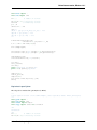
Release 1.2.1
Romain Brette, Dan Goodman
July 06, 2010
CONTENTS
1
Introduction
2
Installation
2.1 Quick installation .
2.2 Manual installation
2.3 Testing . . . . . .
2.4 Optimisations . . .
1
.
.
.
.
5
5
5
6
7
3
Getting started
3.1 Tutorials . . . . . . . . . . . . . . . . . . . . . . . . . . . . . . . . . . . . . . . . . . . . . . . . .
3.2 Examples . . . . . . . . . . . . . . . . . . . . . . . . . . . . . . . . . . . . . . . . . . . . . . . . .
9
9
28
4
User manual
4.1 Units . . . . . . . . . . . . . . .
4.2 Models and neuron groups . . . .
4.3 Connections . . . . . . . . . . .
4.4 Spike-timing-dependent plasticity
4.5 Short-term plasticity . . . . . . .
4.6 Recording . . . . . . . . . . . .
4.7 Inputs . . . . . . . . . . . . . . .
4.8 User-defined operations . . . . .
4.9 Analysis and plotting . . . . . . .
4.10 Realtime control . . . . . . . . .
4.11 Clocks . . . . . . . . . . . . . .
4.12 Simulation control . . . . . . . .
4.13 More on equations . . . . . . . .
4.14 File management . . . . . . . . .
.
.
.
.
.
.
.
.
.
.
.
.
.
.
.
.
.
.
.
.
.
.
.
.
.
.
.
.
.
.
.
.
.
.
.
.
.
.
.
.
.
.
.
.
.
.
.
.
.
.
.
.
.
.
.
.
.
.
.
.
.
.
.
.
.
.
.
.
.
.
.
.
.
.
.
.
.
.
.
.
.
.
.
.
.
.
.
.
.
.
.
.
.
.
.
.
.
.
.
.
.
.
.
.
.
.
.
.
.
.
.
.
.
.
.
.
.
.
.
.
.
.
.
.
.
.
.
.
.
.
.
.
.
.
.
.
.
.
.
.
.
.
.
.
.
.
.
.
.
.
.
.
.
.
.
.
.
.
.
.
.
.
.
.
.
.
.
.
.
.
.
.
.
.
.
.
.
.
.
.
.
.
.
.
.
.
.
.
.
.
.
.
.
.
.
.
.
.
.
.
.
.
.
.
.
.
.
.
.
.
.
.
.
.
.
.
.
.
.
.
.
.
.
.
.
.
.
.
.
.
.
.
.
.
.
.
.
.
.
.
.
.
.
.
.
.
.
.
.
.
.
.
.
.
.
.
.
.
.
.
.
.
.
.
.
.
.
.
.
.
.
.
.
.
.
.
.
.
.
.
.
.
.
.
.
.
.
.
.
.
.
.
.
.
.
.
.
.
.
.
.
.
.
.
.
.
.
.
.
.
.
.
.
.
.
.
.
.
.
.
.
.
.
.
.
.
.
.
.
.
.
.
.
.
.
.
.
.
.
.
.
.
.
.
.
.
.
.
.
.
.
.
.
.
.
.
.
.
.
.
.
.
.
.
.
.
.
.
.
.
.
.
.
.
.
.
.
.
.
.
.
.
.
.
.
.
.
.
.
.
.
.
.
.
.
.
.
.
.
.
.
.
.
.
.
.
.
.
.
.
.
.
.
.
.
.
.
.
.
.
.
.
.
.
.
.
.
.
.
.
.
.
.
.
.
.
.
.
.
.
.
.
.
.
.
.
.
.
.
.
.
.
.
.
.
.
.
.
.
.
.
.
.
.
.
.
.
.
.
.
.
.
.
.
.
.
.
.
.
.
.
.
.
.
.
.
.
.
.
.
.
.
.
.
.
.
.
.
.
.
.
.
.
.
91
91
93
98
101
102
103
105
108
109
111
111
112
113
118
The library
5.1 Library models . .
5.2 Random processes
5.3 Electrophysiology
5.4 Model fitting . . .
.
.
.
.
.
.
.
.
.
.
.
.
.
.
.
.
.
.
.
.
.
.
.
.
.
.
.
.
.
.
.
.
.
.
.
.
.
.
.
.
.
.
.
.
.
.
.
.
.
.
.
.
.
.
.
.
.
.
.
.
.
.
.
.
.
.
.
.
.
.
.
.
.
.
.
.
.
.
.
.
.
.
.
.
.
.
.
.
.
.
.
.
.
.
.
.
.
.
.
.
.
.
.
.
.
.
.
.
.
.
.
.
.
.
.
.
.
.
.
.
.
.
.
.
.
.
.
.
.
.
.
.
.
.
.
.
.
.
.
.
.
.
.
.
119
119
123
123
127
Advanced concepts
6.1 How to write efficient Brian code . . .
6.2 Compiled code . . . . . . . . . . . . .
6.3 Projects with multiple files or functions
6.4 Connection matrices . . . . . . . . . .
6.5 Parameters . . . . . . . . . . . . . . .
.
.
.
.
.
.
.
.
.
.
.
.
.
.
.
.
.
.
.
.
.
.
.
.
.
.
.
.
.
.
.
.
.
.
.
.
.
.
.
.
.
.
.
.
.
.
.
.
.
.
.
.
.
.
.
.
.
.
.
.
.
.
.
.
.
.
.
.
.
.
.
.
.
.
.
.
.
.
.
.
.
.
.
.
.
.
.
.
.
.
.
.
.
.
.
.
.
.
.
.
.
.
.
.
.
.
.
.
.
.
.
.
.
.
.
.
.
.
.
.
.
.
.
.
.
.
.
.
.
.
.
.
.
.
.
.
.
.
.
.
.
.
.
.
.
.
.
.
.
.
.
.
.
.
.
.
.
.
.
.
.
.
.
.
.
131
131
133
134
135
136
5
6
.
.
.
.
.
.
.
.
.
.
.
.
.
.
.
.
.
.
.
.
.
.
.
.
.
.
.
.
.
.
.
.
.
.
.
.
.
.
.
.
.
.
.
.
.
.
.
.
.
.
.
.
.
.
.
.
.
.
.
.
.
.
.
.
.
.
.
.
.
.
.
.
.
.
.
.
.
.
.
.
.
.
.
.
.
.
.
.
.
.
.
.
.
.
.
.
.
.
.
.
.
.
.
.
.
.
.
.
.
.
.
.
.
.
.
.
.
.
.
.
.
.
.
.
.
.
.
.
.
.
.
.
.
.
.
.
.
.
.
.
.
.
.
.
.
.
.
.
.
.
.
.
.
.
.
.
.
.
.
.
.
.
.
.
.
.
.
.
.
.
.
.
.
.
.
.
.
.
.
.
.
.
.
.
.
.
.
.
.
.
.
.
.
.
.
.
.
.
.
.
.
.
.
.
i
6.6
6.7
6.8
Precalculated tables . . . . . . . . . . . . . . . . . . . . . . . . . . . . . . . . . . . . . . . . . . . 137
Preferences . . . . . . . . . . . . . . . . . . . . . . . . . . . . . . . . . . . . . . . . . . . . . . . . 138
Logging . . . . . . . . . . . . . . . . . . . . . . . . . . . . . . . . . . . . . . . . . . . . . . . . . . 139
7
Extending Brian
8
Reference
8.1 SciPy, NumPy and PyLab
8.2 Units system . . . . . . .
8.3 Clocks . . . . . . . . . .
8.4 Neuron models and groups
8.5 Integration . . . . . . . .
8.6 Standard Groups . . . . .
8.7 Connections . . . . . . .
8.8 Plasticity . . . . . . . . .
8.9 Network . . . . . . . . .
8.10 Monitors . . . . . . . . .
8.11 Plotting . . . . . . . . . .
8.12 Variable updating . . . . .
8.13 Analysis . . . . . . . . .
8.14 Remote control . . . . . .
8.15 Progress reporting . . . .
8.16 Model fitting toolbox . . .
8.17 Magic in Brian . . . . . .
8.18 Tests . . . . . . . . . . .
9
141
.
.
.
.
.
.
.
.
.
.
.
.
.
.
.
.
.
.
.
.
.
.
.
.
.
.
.
.
.
.
.
.
.
.
.
.
.
.
.
.
.
.
.
.
.
.
.
.
.
.
.
.
.
.
.
.
.
.
.
.
.
.
.
.
.
.
.
.
.
.
.
.
.
.
.
.
.
.
.
.
.
.
.
.
.
.
.
.
.
.
.
.
.
.
.
.
.
.
.
.
.
.
.
.
.
.
.
.
.
.
.
.
.
.
.
.
.
.
.
.
.
.
.
.
.
.
.
.
.
.
.
.
.
.
.
.
.
.
.
.
.
.
.
.
.
.
.
.
.
.
.
.
.
.
.
.
.
.
.
.
.
.
.
.
.
.
.
.
.
.
.
.
.
.
.
.
.
.
.
.
.
.
.
.
.
.
.
.
.
.
.
.
.
.
.
.
.
.
.
.
.
.
.
.
.
.
.
.
.
.
.
.
.
.
.
.
.
.
.
.
.
.
.
.
.
.
.
.
.
.
.
.
.
.
.
.
.
.
.
.
.
.
.
.
.
.
.
.
.
.
.
.
.
.
.
.
.
.
.
.
.
.
.
.
.
.
.
.
.
.
.
.
.
.
.
.
.
.
.
.
.
.
.
.
.
.
.
.
.
.
.
.
.
.
.
.
.
.
.
.
.
.
.
.
.
.
.
.
.
.
.
.
.
.
.
.
.
.
.
.
.
.
.
.
.
.
.
.
.
.
.
.
.
.
.
.
.
.
.
.
.
.
.
.
.
.
.
.
.
.
.
.
.
.
.
.
.
.
.
.
.
.
.
.
.
.
.
.
.
.
.
.
.
.
.
.
.
.
.
.
.
.
.
.
.
.
.
.
.
.
.
.
.
.
.
.
.
.
.
.
.
.
.
.
.
.
.
.
.
.
.
.
.
.
.
.
.
.
.
.
.
.
.
.
.
.
.
.
.
.
.
.
.
.
.
.
.
.
.
.
.
.
.
.
.
.
.
.
.
.
.
.
.
.
.
.
.
.
.
.
.
.
.
.
.
.
.
.
.
.
.
.
.
.
.
.
.
.
.
.
.
.
.
.
.
.
.
.
.
.
.
.
.
.
.
.
.
.
.
.
.
.
.
.
.
.
.
.
.
.
.
.
.
.
.
.
.
.
.
.
.
.
.
.
.
.
.
.
.
.
.
.
.
.
.
.
.
.
.
.
.
.
.
.
.
.
.
.
.
.
.
.
.
.
.
.
.
.
.
.
.
.
.
.
.
.
.
.
.
.
.
.
.
.
.
.
.
.
.
.
.
.
.
.
.
.
.
.
.
.
.
.
.
.
.
.
.
.
.
.
.
.
.
.
.
.
.
.
.
.
.
.
.
.
.
.
.
.
.
.
.
.
.
.
.
.
.
.
.
.
.
.
.
.
.
.
.
.
.
.
.
.
.
.
.
.
.
.
.
.
.
.
.
.
.
.
.
.
.
.
.
.
.
.
.
.
.
.
.
.
.
.
.
.
.
.
.
.
.
.
.
.
.
.
.
.
.
.
.
.
.
.
.
.
.
.
.
.
.
.
.
.
.
.
.
.
.
.
.
.
.
.
.
.
.
.
.
.
.
.
143
143
143
145
147
153
154
156
162
164
169
175
176
178
179
180
181
183
185
Typical Tasks
187
9.1 Projects with multiple files or functions . . . . . . . . . . . . . . . . . . . . . . . . . . . . . . . . . 187
10 Experimental features
189
10.1 Automatic C code generation for nonlinear state updaters . . . . . . . . . . . . . . . . . . . . . . . 189
10.2 Multilinear state updater . . . . . . . . . . . . . . . . . . . . . . . . . . . . . . . . . . . . . . . . . 189
11 Developer’s guide
11.1 Guidelines . . . . . . .
11.2 Simulation principles . .
11.3 Main code structure . .
11.4 Equations . . . . . . . .
11.5 Brian package structure
11.6 Repository structure . .
.
.
.
.
.
.
.
.
.
.
.
.
.
.
.
.
.
.
.
.
.
.
.
.
.
.
.
.
.
.
.
.
.
.
.
.
.
.
.
.
.
.
.
.
.
.
.
.
.
.
.
.
.
.
.
.
.
.
.
.
.
.
.
.
.
.
.
.
.
.
.
.
.
.
.
.
.
.
.
.
.
.
.
.
.
.
.
.
.
.
.
.
.
.
.
.
.
.
.
.
.
.
.
.
.
.
.
.
.
.
.
.
.
.
.
.
.
.
.
.
.
.
.
.
.
.
.
.
.
.
.
.
.
.
.
.
.
.
.
.
.
.
.
.
.
.
.
.
.
.
.
.
.
.
.
.
.
.
.
.
.
.
.
.
.
.
.
.
.
.
.
.
.
.
.
.
.
.
.
.
.
.
.
.
.
.
.
.
.
.
.
.
.
.
.
.
.
.
.
.
.
.
.
.
.
.
.
.
.
.
.
.
.
.
.
.
.
.
.
.
.
.
.
.
.
.
.
.
.
.
.
.
.
.
.
.
.
.
.
.
.
.
.
.
.
.
191
191
192
196
200
204
205
Module Index
207
Index
209
ii
CHAPTER
ONE
INTRODUCTION
Brian is a clock driven simulator for spiking neural networks, written in the Python programming language.
The simulator is written almost entirely in Python. The idea is that it can be used at various levels of abstraction
without the steep learning curve of software like Neuron, where you have to learn their own programming language
to extend their models. As a language, Python is well suited to this task because it is easy to learn, well known and
supported, and allows a great deal of flexibility in usage and in designing interfaces and abstraction mechanisms. As
an interpreted language, and therefore slower than say C++, Python is not the obvious choice for writing a computationally demanding scientific application. However, the SciPy module for Python provides very efficient linear algebra
routines, which means that vectorised code can be very fast.
Here’s what the Python web site has to say about themselves:
Python is an easy to learn, powerful programming language. It has efficient high-level data structures and
a simple but effective approach to object-oriented programming. Python’s elegant syntax and dynamic
typing, together with its interpreted nature, make it an ideal language for scripting and rapid application
development in many areas on most platforms.
The Python interpreter and the extensive standard library are freely available in source or binary form for
all major platforms from the Python Web site, http://www.python.org/, and may be freely distributed. The
same site also contains distributions of and pointers to many free third party Python modules, programs
and tools, and additional documentation.
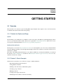
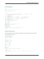
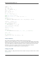
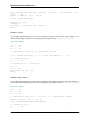
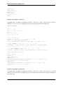
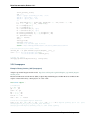
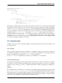
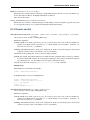
As an example of the ease of use and clarity of programs written in Brian, the following script defines and runs a
randomly connected network of 4000 integrate and fire neurons with exponential currents:
from brian import *
eqs=’’’
dv/dt = (ge+gi-(v+49*mV))/(20*ms) : volt
dge/dt = -ge/(5*ms) : volt
dgi/dt = -gi/(10*ms) : volt
’’’
P=NeuronGroup(4000,model=eqs,threshold=-50*mV,reset=-60*mV)
P.v=-60*mV
Pe=P.subgroup(3200)
Pi=P.subgroup(800)
Ce=Connection(Pe,P,’ge’,weight=1.62*mV,sparseness=0.02)
Ci=Connection(Pi,P,’gi’,weight=-9*mV,sparseness=0.02)
M=SpikeMonitor(P)
run(1*second)
raster_plot(M)
show()
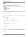
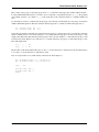
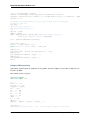
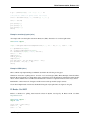
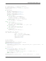
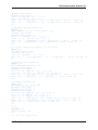
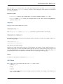
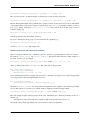
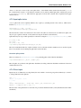
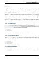
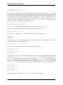
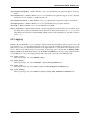
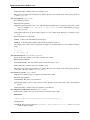
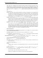
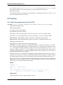
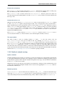
As an example of the output of Brian, the following two images reproduce figures from Diesmann et al. 1999 on
synfire chains. The first is a raster plot of a synfire chain showing the stabilisation of the chain.
1
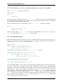
Brian Documentation, Release 1.2.1
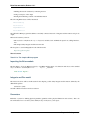
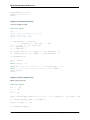
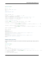
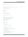
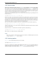
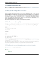
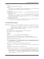
The simulation of 1000 neurons in 10 layers, each all-to-all connected to the next, using integrate and fire neurons with
synaptic noise for 100ms of simulated time took 1 second to run with a timestep of 0.1ms on a 2.4GHz Intel Xeon
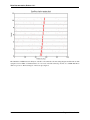
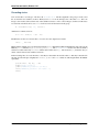
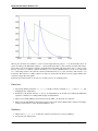
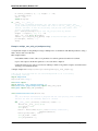
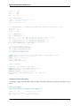
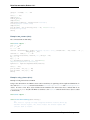
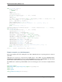
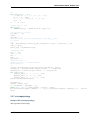
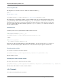
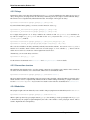
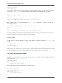
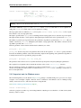
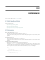
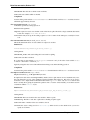
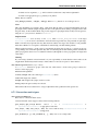
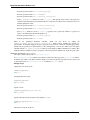
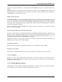
dual-core processor. The next image is of the state space, figure 3:
2
Chapter 1. Introduction
Brian Documentation, Release 1.2.1
The figure computed 50 averages for each of 121 starting points over 100ms at a timestep of 0.1ms and took 201s to
run on the same processor as above.
3
Brian Documentation, Release 1.2.1
4
Chapter 1. Introduction
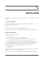
CHAPTER
TWO
INSTALLATION
If you already have a copy of Python 2.5 or 2.6, try the Quick installation below, otherwise take a look at Manual
installation.
2.1 Quick installation
The easiest way to install Brian if you already have a version of Python 2.5 or 2.6 including the easy_install
script is to simply run the following in a shell:
easy_install brian
This will download and install Brian and all its required packages (NumPy, SciPy, etc.).
Note that there are some optimisations you can make after installation, see the section below on Optimisations.
2.2 Manual installation
Installing Brian requires the following components:
1. Python version 2.5 or 2.6.
2. NumPy and Scipy packages for Python: an efficient scientific library.
3. PyLab package for Python: a plotting library similar to Matlab (see the detailed installation instructions).
4. SymPy package for Python: a library for symbolic mathematics (not mandatory yet for Brian).
5. Brian itself (don’t forget to download the extras.zip file, which includes examples, tutorials, and a complete
copy of the documentation). Brian is also a Python package and can be installed as explained below.
Fortunately, Python packages are very quick and easy to install, so the whole process shouldn’t take very long.
We also recommend using the following for writing programs in Python (see details below):
1. Eclipse IDE with PyDev
2. IPython shell
Finally, if you want to use the (optional) automatic C++ code generation features of Brian, you should have the gcc
compiler installed (on Cygwin if you are running on Windows).
Mac users: the Scipy Superpack for Intel OS X includes recent versions of Numpy, Scipy, Pylab and IPython.
5
Brian Documentation, Release 1.2.1
Windows users: the Python(x,y) distribution includes all the packages (including Eclipse and IPython) above except
Brian (which is available as an optional plugin).
2.2.1 Installing Python packages
On Windows, Python packages (including Brian) are generally installed simply by running an .exe file. On other
operating systems, you can download the source release (typically a compressed archive .tar.gz or .zip that you need
to unzip) and then install the package by typing the following in your shell:
python setup.py install
2.2.2 Installing Eclipse
Eclipse is an Integrated Development Environment (IDE) for any programming language. PyDev is a plugin for
Eclipse with features specifically for Python development. The combination of these two is excellent for Python
development (it’s what we use for writing Brian).
To install Eclipse, go to their web page and download any of the base language IDEs. It doesn’t matter which one, but
Python is not one of the base languages so you have to choose an alternative language. Probably the most useful is the
C++ one or the Java one. The C++ one can be downloaded here.
Having downloaded and installed Eclipse, you should download and install the PyDev plugin from their web site. The
best way to do this is directly from within the Eclipse IDE. Follow the instructions on the PyDev manual page.
2.2.3 Installing IPython
IPython is an interactive shell for Python. It has features for SciPy and PyLab built in, so it is a good choice for
scientific work. Download from their page. If you are using Windows, you will also need to download PyReadline
from the same page.
2.2.4 C++ compilers
The default for Brian is to use the gcc compiler which will be installed already on most unix or linux distributions. If
you are using Windows, you can install cygwin (make sure to include the gcc package). Alternatively, some but not
all versions of Microsoft Visual C++ should be compatible, but this is untested so far. See the documentation for the
SciPy Weave package for more information on this. See also the section on Compiled code.
2.3 Testing
You can test whether Brian has installed properly by running Python and typing the following two lines:
from brian import *
brian_sample_run()
A sample network should run and produce a raster plot.
6
Chapter 2. Installation
Brian Documentation, Release 1.2.1
2.4 Optimisations
After a successful installation, there are some optimisations you can make to your Brian installation to get it running
faster using compiled C code. We do not include these as standard because they do not work on all computers, and
we want Brian to install without problems on all computers. Note that including all the optimisations can result in
significant speed increases (around 30%).
These optimisations are described in detail in the section on Compiled code.
2.4. Optimisations
7
Brian Documentation, Release 1.2.1
8
Chapter 2. Installation
CHAPTER
THREE
GETTING STARTED
3.1 Tutorials
These tutorials cover some basic topics in writing Brian scripts in Python. The complete source code for the tutorials
is available in the tutorials folder in the extras package.
3.1.1 Tutorials for Python and Scipy
Python
The first thing to do in learning how to use Brian is to have a basic grasp of the Python programming language. There
are lots of good tutorials already out there. The best one is probably the official Python tutorial. There is also a course
for biologists at the Pasteur Institute: Introduction to programming using Python.
NumPy, SciPy and Pylab
The first place to look is the SciPy documentation website. To start using Brian, you do not need to understand much
about how NumPy and SciPy work, although understanding how their array structures work will be useful for more
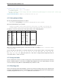
advanced uses of Brian.
The syntax of the Numpy and Pylab functions is very similar to Matlab. If you already know Matlab, you could read
this tutorial: NumPy for Matlab users and this list of Matlab-Python translations (pdf version here). A tutorial is also
available on the web site of Pylab.
3.1.2 Tutorial 1: Basic Concepts
In this tutorial, we introduce some of the basic concepts of a Brian simulation:
• Importing the Brian module into Python
• Using quantities with units
• Defining a neuron model by its differential equation
• Creating a group of neurons
• Running a network
• Looking at the output of the network
• Modifying the state variables of the network directly
9
Brian Documentation, Release 1.2.1
• Defining the network structure by connecting neurons
• Doing a raster plot of the output
• Plotting the membrane potential of an individual neuron
The following Brian classes will be introduced:
• NeuronGroup
• Connection
• SpikeMonitor
• StateMonitor
We will build a Brian program that defines a randomly connected network of integrate and fire neurons and plot its
output.
This tutorial assumes you know:
• The very basics of Python, the import keyword, variables, basic arithmetical expressions, calling functions,
lists
• The simplest leaky integrate and fire neuron model
The best place to start learning Python is the official tutorial:
http://docs.python.org/tut/
Tutorial contents
Tutorial 1a: The simplest Brian program
Importing the Brian module
The first thing to do in any Brian program is to load Brian and the names of its functions and classes. The standard
way to do this is to use the Python from ... import * statement.
from brian import *
Integrate and Fire model
The neuron model we will use in this tutorial is the simplest possible leaky integrate and fire neuron, defined by the
differential equation:
tau dV/dt = -(V-El)
and with a threshold value Vt and reset value Vr.
Parameters
Brian has a system for defining physical quantities (quantities with a physical dimension such as time). The code
below illustrates how to use this system, which (mostly) works just as you’d expect.
10
Chapter 3. Getting started
Brian Documentation, Release 1.2.1
tau = 20
Vt = -50
Vr = -60
El = -60
*
*
*
*
msecond
mvolt
mvolt
mvolt
#
#
#
#
membrane time constant
spike threshold
reset value
resting potential (same as the reset)
The built in standard units in Brian consist of all the fundamental SI units like second and metre, along with a selection
of derived SI units such as volt, farad, coulomb. All names are lowercase following the SI standard. In addition, there
are scaled versions of these units using the standard SI prefixes m=1/1000, K=1000, etc.
Neuron model and equations
The simplest way to define a neuron model in Brian is to write a list of the differential equations that define it. For
the moment, we’ll just give the simplest possible example, a single differential equation. You write it in the following
form:
dx/dt = f(x) : unit
where x is the name of the variable, f(x) can be any valid Python expression, and unit is the physical units of the
variable x. In our case we will write:
dV/dt = -(V-El)/tau : volt
to define the variable V with units volt.
To complete the specification of the model, we also define a threshold and reset value and create a group of 40 neurons
with this model.
G = NeuronGroup(N=40, model=’dV/dt = -(V-El)/tau : volt’,
threshold=Vt, reset=Vr)
The statement creates a new object ‘G’ which is an instance of the Brian class NeuronGroup, initialised with the
values in the line above and 40 neurons. In Python, you can call a function or initialise a class using keyword arguments
as well as ordered arguments, so if I defined a function f(x,y) I could call it as f(1,2) or as f(y=2,x=1) and
get the same effect. See the Python tutorial for more information on this.
For the moment, we leave the neurons in this group unconnected to each other, each evolves separately from the others.
Simulation
Finally, we run the simulation for 1 second of simulated time. By default, the simulator uses a timestep dt = 0.1 ms.
run(1 * second)
And that’s it! To see some of the output of this network, go to the next part of the tutorial.
Exercise
The units system of Brian is useful for ensuring that everything is consistent, and that you don’t make hard to find
mistakes in your code by using the wrong units. Try changing the units of one of the parameters and see what happens.
3.1. Tutorials
11
Brian Documentation, Release 1.2.1
Solution
You should see an error message with a Python traceback (telling you which functions were being called when the
error happened), ending in a line something like:
Brian.units.DimensionMismatchError: The differential equations
are not homogeneous!, dimensions were (m^2 kg s^-3 A^-1)
(m^2 kg s^-4 A^-1)
Tutorial 1b: Counting spikes
In the previous part of the tutorial we looked at the following:
• Importing the Brian module into Python
• Using quantities with units
• Defining a neuron model by its differential equation
• Creating a group of neurons
• Running a network
In this part, we move on to looking at the output of the network.
The first part of the code is the same.
from brian import *
tau = 20
Vt = -50
Vr = -60
El = -60
*
*
*
*
msecond
mvolt
mvolt
mvolt
#
#
#
#
membrane time constant
spike threshold
reset value
resting potential (same as the reset)
G = NeuronGroup(N=40, model=’dV/dt = -(V-El)/tau : volt’,
threshold=Vt, reset=Vr)
Counting spikes
Now we would like to have some idea of what this network is doing. In Brian, we use monitors to keep track of
the behaviour of the network during the simulation. The simplest monitor of all is the SpikeMonitor, which just
records the spikes from a given NeuronGroup.
M = SpikeMonitor(G)
Results
Now we run the simulation as before:
run(1 * second)
And finally, we print out how many spikes there were:
12
Chapter 3. Getting started
Brian Documentation, Release 1.2.1
print M.nspikes
So what’s going on? Why are there 40 spikes? Well, the answer is that the initial value of the membrane potential for
every neuron is 0 mV, which is above the threshold potential of -50 mV and so there is an initial spike at t=0 and then
it resets to -60 mV and stays there, below the threshold potential. In the next part of this tutorial, we’ll make sure there
are some more spikes to see.
Tutorial 1c: Making some activity
In the previous part of the tutorial we found that each neuron was producing only one spike. In this part, we alter the
model so that some more spikes will be generated. What we’ll do is alter the resting potential El so that it is above
threshold, this will ensure that some spikes are generated. The first few lines remain the same:
from brian import *
tau = 20 * msecond
Vt = -50 * mvolt
Vr = -60 * mvolt
# membrane time constant
# spike threshold
# reset value
But we change the resting potential to -49 mV, just above the spike threshold:
El = -49 * mvolt
# resting potential (same as the reset)
And then continue as before:
G = NeuronGroup(N=40, model=’dV/dt = -(V-El)/tau : volt’,
threshold=Vt, reset=Vr)
M = SpikeMonitor(G)
run(1 * second)
print M.nspikes
Running this program gives the output 840. That’s because every neuron starts at the same initial value and proceeds
deterministically, so that each neuron fires at exactly the same time, in total 21 times during the 1s of the run.
In the next part, we’ll introduce a random element into the behaviour of the network.
Exercises
1. Try varying the parameters and seeing how the number of spikes generated varies.
2. Solve the differential equation by hand and compute a formula for the number of spikes generated. Compare
this with the program output and thereby partially verify it. (Hint: each neuron starts at above the threshold and
so fires a spike immediately.)
Solution
Solving the differential equation gives:
V = El + (Vr-El) exp (-t/tau)
3.1. Tutorials
13
Brian Documentation, Release 1.2.1
Setting V=Vt at time t gives:
t = tau log( (Vr-El) / (Vt-El) )
If the simulator runs for time T, and fires a spike immediately at the beginning of the run it will then generate n spikes,
where:
n = [T/t] + 1
If you have m neurons all doing the same thing, you get nm spikes. This calculation with the parameters above gives:
t = 48.0 ms n = 21 nm = 840
As predicted.
Tutorial 1d: Introducing randomness
In the previous part of the tutorial, all the neurons start at the same values and proceed deterministically, so they all
spike at exactly the same times. In this part, we introduce some randomness by initialising all the membrane potentials
to uniform random values between the reset and threshold values.
We start as before:
from brian import *
tau = 20
Vt = -50
Vr = -60
El = -49
*
*
*
*
msecond
mvolt
mvolt
mvolt
#
#
#
#
membrane time constant
spike threshold
reset value
resting potential (same as the reset)
G = NeuronGroup(N=40, model=’dV/dt = -(V-El)/tau : volt’,
threshold=Vt, reset=Vr)
M = SpikeMonitor(G)
But before we run the simulation, we set the values of the membrane potentials directly. The notation G.V refers to the
array of values for the variable V in group G. In our case, this is an array of length 40. We set its values by generating
an array of random numbers using Brian’s rand function. The syntax is rand(size) generates an array of length
size consisting of uniformly distributed random numbers in the interval 0, 1.
G.V = Vr + rand(40) * (Vt - Vr)
And now we run the simulation as before.
run(1 * second)
print M.nspikes
But this time we get a varying number of spikes each time we run it, roughly between 800 and 850 spikes. In the next
part of this tutorial, we introduce a bit more interest into this network by connecting the neurons together.
Tutorial 1e: Connecting neurons
In the previous parts of this tutorial, the neurons are still all unconnected. We add in connections here. The model we
use is that when neuron i is connected to neuron j and neuron i fires a spike, then the membrane potential of neuron j
is instantaneously increased by a value psp. We start as before:
14
Chapter 3. Getting started
Brian Documentation, Release 1.2.1
from brian import *
tau = 20
Vt = -50
Vr = -60
El = -49
*
*
*
*
msecond
mvolt
mvolt
mvolt
#
#
#
#
membrane time constant
spike threshold
reset value
resting potential (same as the reset)
Now we include a new parameter, the PSP size:
psp = 0.5 * mvolt
# postsynaptic potential size
And continue as before:
G = NeuronGroup(N=40, model=’dV/dt = -(V-El)/tau : volt’,
threshold=Vt, reset=Vr)
Connections
We now proceed to connect these neurons. Firstly, we declare that there is a connection from neurons in G to neurons
in G. For the moment, this is just something that is necessary to do, the reason for doing it this way will become clear
in the next tutorial.
C = Connection(G, G)
Now the interesting part, we make these neurons be randomly connected with probability 0.1 and weight psp. Each
neuron i in G will be connected to each neuron j in G with probability 0.1. The weight of the connection is the amount
that is added to the membrane potential of the target neuron when the source neuron fires a spike.
C.connect_random(sparseness=0.1, weight=psp)
These two previous lines could be done in one line:
C = Connection(G,G,sparseness=0.1,weight=psp)
Now we continue as before:
M = SpikeMonitor(G)
G.V = Vr + rand(40) * (Vt - Vr)
run(1 * second)
print M.nspikes
You can see that the number of spikes has jumped from around 800-850 to around 1000-1200. In the next part of the
tutorial, we’ll look at a way to plot the output of the network.
Exercise
Try varying the parameter psp and see what happens. How large can you make the number of spikes output by the
network? Why?
3.1. Tutorials
15
Brian Documentation, Release 1.2.1
Solution
The logically maximum number of firings is 400,000 = 40 * 1000 / 0.1, the number of neurons in the network * the
time it runs for / the integration step size (you cannot have more than one spike per step).
In fact, the number of firings is bounded above by 200,000. The reason for this is that the network updates in the
following way:
1. Integration step
2. Find neurons above threshold
3. Propagate spikes
4. Reset neurons which spiked
You can see then that if neuron i has spiked at time t, then it will not spike at time t+dt, even if it receives spikes from
another neuron. Those spikes it receives will be added at step 3 at time t, then reset to Vr at step 4 of time t, then
the thresholding function at time t+dt is applied at step 2, before it has received any subsequent inputs. So the most a
neuron can spike is every other time step.
Tutorial 1f: Recording spikes
In the previous part of the tutorial, we defined a network with not entirely trivial behaviour, and printed the number of
spikes. In this part, we’ll record every spike that the network generates and display a raster plot of them. We start as
before:
from brian import *
tau = 20 * msecond
Vt = -50 * mvolt
Vr = -60 * mvolt
El = -49 * mvolt
psp = 0.5 * mvolt
#
#
#
#
#
membrane time constant
spike threshold
reset value
resting potential (same as the reset)
postsynaptic potential size
G = NeuronGroup(N=40, model=’dV/dt = -(V-El)/tau : volt’,
threshold=Vt, reset=Vr)
C = Connection(G, G)
C.connect_random(sparseness=0.1, weight=psp)
M = SpikeMonitor(G)
G.V = Vr + rand(40) * (Vt - Vr)
run(1 * second)
print M.nspikes
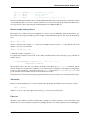
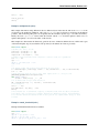
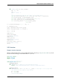
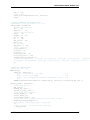
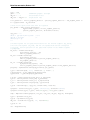
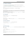
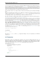
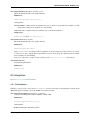
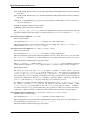
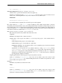
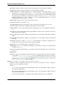
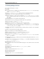
Having run the network, we simply use the raster_plot() function provided by Brian. After creating plots, we
have to use the show() function to display them. This function is from the PyLab module that Brian uses for its built
in plotting routines.
raster_plot()
show()
16
Chapter 3. Getting started
Brian Documentation, Release 1.2.1
As you can see, despite having introduced some randomness into our network, the output is very regular indeed. In
the next part we introduce one more way to plot the output of a network.
Tutorial 1g: Recording membrane potentials
In the previous part of this tutorial, we plotted a raster plot of the firing times of the network. In this tutorial, we
introduce a way to record the value of the membrane potential for a neuron during the simulation, and plot it. We
continue as before:
from brian import *
tau = 20 * msecond
Vt = -50 * mvolt
Vr = -60 * mvolt
El = -49 * mvolt
psp = 0.5 * mvolt
#
#
#
#
#
membrane time constant
spike threshold
reset value
resting potential (same as the reset)
postsynaptic potential size
G = NeuronGroup(N=40, model=’dV/dt = -(V-El)/tau : volt’,
threshold=Vt, reset=Vr)
C = Connection(G, G)
C.connect_random(sparseness=0.1, weight=psp)
This time we won’t record the spikes.
3.1. Tutorials
17
Brian Documentation, Release 1.2.1
Recording states
Now we introduce a second type of monitor, the StateMonitor. The first argument is the group to monitor, and
the second is the state variable to monitor. The keyword record can be an integer, list or the value True. If it is an
integer i, the monitor will record the state of the variable for neuron i. If it’s a list of integers, it will record the states
for each neuron in the list. If it’s set to True it will record for all the neurons in the group.
M = StateMonitor(G, ’V’, record=0)
And then we continue as before:
G.V = Vr + rand(40) * (Vt - Vr)
But this time we run it for a shorter time so we can look at the output in more detail:
run(200 * msecond)
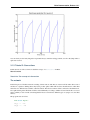
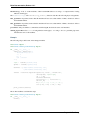
Having run the simulation, we plot the results using the plot command from PyLab which has the same syntax as the
Matlab plot‘ command, i.e. plot(xvals,yvals,...). The StateMonitor monitors the times at which it
monitored a value in the array M.times, and the values in the array M[0]. The notation M[i] means the array of
values of the monitored state variable for neuron i.
In the following lines, we scale the times so that they’re measured in ms and the values so that they’re measured in
mV. We also label the plot using PyLab’s xlabel, ylabel and title functions, which again mimic the Matlab
equivalents.
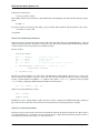
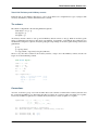
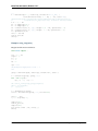
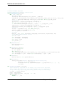
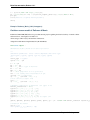
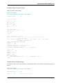
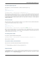
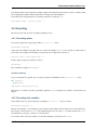
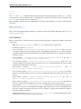
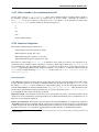
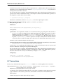
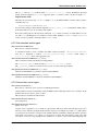
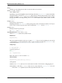
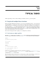
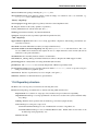
plot(M.times / ms, M[0] / mV)
xlabel(’Time (in ms)’)
ylabel(’Membrane potential (in mV)’)
title(’Membrane potential for neuron 0’)
show()
18
Chapter 3. Getting started
Brian Documentation, Release 1.2.1
You can clearly see the leaky integration exponential decay toward the resting potential, as well as the jumps when a
spike was received.
3.1.3 Tutorial 2: Connections
In this tutorial, we will cover in more detail the concept of a Connection in Brian.
Tutorial contents
Tutorial 2a: The concept of a Connection
The network
In this first part, we’ll build a network consisting of three neurons. The first two neurons will be under direct control
and have no equations defining them, they’ll just produce spikes which will feed into the third neuron. This third
neuron has two different state variables, called Va and Vb. The first two neurons will be connected to the third neuron,
but a spike arriving at the third neuron will be treated differently according to whether it came from the first or second
neuron (which you can consider as meaning that the first two neurons have different types of synapses on to the third
neuron).
The program starts as follows.
from brian import *
tau_a = 1 * ms
tau_b = 10 * ms
3.1. Tutorials
19
Brian Documentation, Release 1.2.1
Vt = 10 * mV
Vr = 0 * mV
Differential equations
This time, we will have multiple differential equations. We will use the Equations object, although you could
equally pass the multi-line string defining the differential equations directly when initialising the NeuronGroup
object (see the next part of the tutorial for an example of this).
eqs = Equations(’’’
dVa/dt = -Va/tau_a : volt
dVb/dt = -Vb/tau_b : volt
’’’)
So far, we have defined a model neuron with two state variables, Va and Vb, which both decay exponentially towards
0, but with different time constants tau_a and tau_b. This is just so that you can see the difference between them
more clearly in the plot later on.
SpikeGeneratorGroup
Now we introduce the SpikeGeneratorGroup class. This is a group of neurons without a model, which just
produces spikes at the times that you specify. You create a group like this by writing:
G = SpikeGeneratorGroup(N,spiketimes)
where N is the number of neurons in the group, and spiketimes is a list of pairs (i,t) indicating that neuron i
should fire at time t. In fact, spiketimes can be any ‘iterable container’ or ‘generator’, but we don’t cover that
here (see the detailed documentation for SpikeGeneratorGroup).
In our case, we want to create a group with two neurons, the first of which (neuron 0) fires at times 1 ms and 4 ms, and
the second of which (neuron 1) fires at times 2 ms and 3 ms. The list of spiketimes then is:
spiketimes = [(0, 1 * ms), (0, 4 * ms),
(1, 2 * ms), (1, 3 * ms)]
and we create the group as follows:
G1 = SpikeGeneratorGroup(2, spiketimes)
Now we create a second group, with one neuron, according to the model we defined earlier.
G2 = NeuronGroup(N=1, model=eqs, threshold=Vt, reset=Vr)
Connections
In Brian, a Connection from one NeuronGroup to another is defined by writing:
C = Connection(G,H,state)
20
Chapter 3. Getting started
Brian Documentation, Release 1.2.1
Here G is the source group, H is the target group, and state is the name of the target state variable. When a neuron i
in G fires, Brian finds all the neurons j in H that i in G is connected to, and adds the amount C[i,j] to the specified
state variable of neuron j in H. Here C[i,j] is the (i,j)th entry of the connection matrix of C (which is initially all
zero).
To start with, we create two connections from the group of two directly controlled neurons to the group of one neuron
with the differential equations. The first connection has the target state Va and the second has the target state Vb.
C1 = Connection(G1, G2, ’Va’)
C2 = Connection(G1, G2, ’Vb’)
So far, this only declares our intention to connect neurons in group G1 to neurons in group G2, because the connection
matrix is initially all zeros. Now, with connection C1 we connect neuron 0 in group G1 to neuron 0 in group G2, with
weight 3 mV. This means that when neuron 0 in group G1 fires, the state variable Va of the neuron in group G2 will
be increased by 6 mV. Then we use connection C2 to connection neuron 1 in group G1 to neuron 0 in group G2, this
time with weight 3 mV.
C1[0, 0] = 6 * mV
C2[1, 0] = 3 * mV
The net effect of this is that when neuron 0 of G1 fires, Va for the neuron in G2 will increase 6 mV, and when neuron
1 of G1 fires, Vb for the neuron in G2 will increase 3 mV.
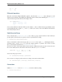
Now we set up monitors to record the activity of the network, run it and plot it.
Ma = StateMonitor(G2, ’Va’, record=True)
Mb = StateMonitor(G2, ’Vb’, record=True)
run(10 * ms)
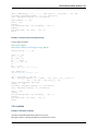
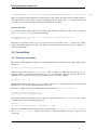
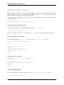
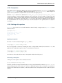
plot(Ma.times, Ma[0])
plot(Mb.times, Mb[0])
show()
3.1. Tutorials
21
Brian Documentation, Release 1.2.1
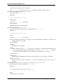
The two plots show the state variables Va and Vb for the single neuron in group G2. Va is shown in blue, and Vb in
green. According to the differential equations, Va decays much faster than Vb (time constant 1 ms rather than 10 ms),
but we have set it up (through the connection strengths) that an incoming spike from neuron 0 of G1 causes a large
increase of 6 mV to Va, whereas a spike from neuron 1 of G1 causes a smaller increase of 3 mV to Vb. The value
for Va then jumps at times 1 ms and 4 ms, when we defined neuron 0 of G1 to fire, and decays almost back to rest
in between. The value for Vb jumps at times 2 ms and 3 ms, and because the times are closer together and the time
constant is longer, they add together.
In the next part of this tutorial, we’ll see how to use this system to do something useful.
Exercises
1. Try playing with the parameters tau_a, tau_b and the connection strengths, C1[0,0] and C2[0,1]. Try
changing the list of spike times.
2. In this part of the tutorial, the states Va and Vb are independent of one another. Try rewriting the differential
equations so that they’re not independent and play around with that.
3. Write a network with inhibitory and excitatory neurons. Hint: you only need one connection.
4. Write a network with inhibitory and excitatory neurons whose actions have different time constants (for example,
excitatory neurons have a slower effect than inhibitory ones).
Solutions
1. Simple write C[i,j]=-3*mV to make the connection from neuron i to neuron j inhibitory.
2. See the next part of this tutorial.
22
Chapter 3. Getting started
Brian Documentation, Release 1.2.1
Tutorial 2b: Excitatory and inhibitory currents
In this tutorial, we use multiple connections to solve a real problem, how to implement two types of synapses with
excitatory and inhibitory currents with different time constants.
The scheme
The scheme we implement is the following diffential equations:
taum dV/dt = -V + ge - gi
taue dge/dt = -ge
taui dgi/dt = -gi
An excitatory neuron connects to state ge, and an inhibitory neuron connects to state gi. When an excitatory spike
arrives, ge instantaneously increases, then decays exponentially. Consequently, V will initially but continuously rise
and then fall. Solving these equations, if V(0)=0, ge(0)=g0 corresponding to an excitatory spike arriving at time 0, and
gi(0)=0 then:
gi = 0
ge = g0 exp(-t/taue)
V = (exp(-t/taum) - exp(-t/taue)) taue g0 / (taum-taue)
We use a very short time constant for the excitatory currents, a longer one for the inhibitory currents, and an even
longer one for the membrane potential.
from brian import *
taum
taue
taui
Vt =
Vr =
= 20 * ms
= 1 * ms
= 10 * ms
10 * mV
0 * mV
eqs = Equations(’’’
dV/dt = (-V+ge-gi)/taum : volt
dge/dt = -ge/taue
: volt
dgi/dt = -gi/taui
: volt
’’’)
Connections
As before, we’ll have a group of two neurons under direct control, the first of which will be excitatory this time, and
the second will be inhibitory. To demonstrate the effect, we’ll have two excitatory spikes reasonably close together,
followed by an inhibitory spike later on, and then shortly after that two excitatory spikes close together.
spiketimes = [(0, 1 * ms), (0, 10 * ms),
(1, 40 * ms),
(0, 50 * ms), (0, 55 * ms)]
G1 = SpikeGeneratorGroup(2, spiketimes)
G2 = NeuronGroup(N=1, model=eqs, threshold=Vt, reset=Vr)
C1 = Connection(G1, G2, ’ge’)
C2 = Connection(G1, G2, ’gi’)
3.1. Tutorials
23
Brian Documentation, Release 1.2.1
The weights are the same - when we increase ge the effect on V is excitatory and when we increase gi the effect on
V is inhibitory.
C1[0, 0] = 3 * mV
C2[1, 0] = 3 * mV
We set up monitors and run as normal.
Mv = StateMonitor(G2, ’V’, record=True)
Mge = StateMonitor(G2, ’ge’, record=True)
Mgi = StateMonitor(G2, ’gi’, record=True)
run(100 * ms)
This time we do something a little bit different when plotting it. We want a plot with two subplots, the top one will
show V, and the bottom one will show both ge and gi. We use the subplot command from pylab which mimics
the same command from Matlab.
figure()
subplot(211)
plot(Mv.times, Mv[0])
subplot(212)
plot(Mge.times, Mge[0])
plot(Mgi.times, Mgi[0])
show()
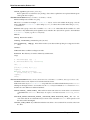
The top figure shows the voltage trace, and the bottom figure shows ge in blue and gi in green. You can see that
although the inhibitory and excitatory weights are the same, the inhibitory current is much more powerful. This is
because the effect of ge or gi on V is related to the integral of the differential equation for those variables, and gi
24
Chapter 3. Getting started
Brian Documentation, Release 1.2.1
decays much more slowly than ge. Thus the size of the negative deflection at 40 ms is much bigger than the excitatory
ones, and even the double excitatory spike after the inhibitory one can’t cancel it out.
In the next part of this tutorial, we set up our first serious network, with 4000 neurons, excitatory and inhibitory.
Exercises
1. Try changing the parameters and spike times to get a feel for how it works.
2. Try an equivalent implementation with the equation taum dV/dt = -V+ge+gi
3. Verify that the differential equation has been solved correctly.
Solutions
Solution for 2:
Simply use the line C2[1,0] = -3*mV to get the same effect.
Solution for 3:
First, set up the situation we described at the top for which we already know the solution of the differential equations,
by changing the spike times as follows:
spiketimes = [(0,0*ms)]
Now we compute what the values ought to be as follows:
t = Mv.times
Vpredicted = (exp(-t/taum) - exp(-t/taue))*taue*(3*mV) / (taum-taue)
Now we can compute the difference between the predicted and actual values:
Vdiff = abs(Vpredicted - Mv[0])
This should be zero:
print max(Vdiff)
Sure enough, it’s as close as you can expect on a computer. When I run this it gives me the value 1.3 aV, which is 1.3
* 10^-18 volts, i.e. effectively zero given the finite precision of the calculations involved.
Tutorial 2c: The CUBA network
In this part of the tutorial, we set up our first serious network that actually does something. It implements the CUBA
network, Benchmark 2 from:
Simulation of networks of spiking neurons: A review of tools and strategies (2006). Brette, Rudolph,
Carnevale, Hines, Beeman, Bower, Diesmann, Goodman, Harris, Zirpe, Natschlager, Pecevski, Ermentrout, Djurfeldt, Lansner, Rochel, Vibert, Alvarez, Muller, Davison, El Boustani and Destexhe. Journal of
Computational Neuroscience
This is a network of 4000 neurons, of which 3200 excitatory, and 800 inhibitory, with exponential synaptic currents.
The neurons are randomly connected with probability 0.02.
3.1. Tutorials
25
Brian Documentation, Release 1.2.1
from brian import *
taum
taue
taui
Vt =
Vr =
El =
we =
wi =
= 20 * ms
# membrane time constant
= 5 * ms
# excitatory synaptic time constant
= 10 * ms
# inhibitory synaptic time constant
-50 * mV
# spike threshold
-60 * mV
# reset value
-49 * mV
# resting potential
(60 * 0.27 / 10) * mV # excitatory synaptic weight
(20 * 4.5 / 10) * mV # inhibitory synaptic weight
eqs = Equations(’’’
dV/dt = (ge-gi-(V-El))/taum : volt
dge/dt = -ge/taue
: volt
dgi/dt = -gi/taui
: volt
’’’)
So far, this has been pretty similar to the previous part, the only difference is we have a couple more parameters, and
we’ve added a resting potential El into the equation for V.
Now we make lots of neurons:
G = NeuronGroup(4000, model=eqs, threshold=Vt, reset=Vr)
Next, we divide them into subgroups. The subgroup() method of a NeuronGroup returns a new NeuronGroup
that can be used in exactly the same way as its parent group. At the moment, the subgrouping mechanism can only
be used to create contiguous groups of neurons (so you can’t have a subgroup consisting of neurons 0-100 and also
200-300 say). We designate the first 3200 neurons as Ge and the second 800 as Gi, these will be the excitatory and
inhibitory neurons.
Ge = G.subgroup(3200) # Excitatory neurons
Gi = G.subgroup(800) # Inhibitory neurons
Now we define the connections. As in the previous part of the tutorial, ge is the excitatory current and gi is the
inhibitory one. Ce says that an excitatory neuron can synapse onto any neuron in G, be it excitatory or inhibitory.
Similarly for inhibitory neurons. We also randomly connect Ge and Gi to the whole of G with probability 0.02 and
the weights given in the list of parameters at the top.
Ce = Connection(Ge, G, ’ge’, sparseness=0.02, weight=we)
Ci = Connection(Gi, G, ’gi’, sparseness=0.02, weight=wi)
Set up some monitors as usual. The line record=0 in the StateMonitor declarations indicates that we only want
to record the activity of neuron 0. This saves time and memory.
M = SpikeMonitor(G)
MV = StateMonitor(G, ’V’, record=0)
Mge = StateMonitor(G, ’ge’, record=0)
Mgi = StateMonitor(G, ’gi’, record=0)
And in order to start the network off in a somewhat more realistic state, we initialise the membrane potentials uniformly
randomly between the reset and the threshold.
G.V = Vr + (Vt - Vr) * rand(len(G))
Now we run.
26
Chapter 3. Getting started
Brian Documentation, Release 1.2.1
run(500 * ms)
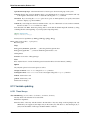
And finally we plot the results. Just for fun, we do a rather more complicated plot than we’ve been doing so far, with
three subplots. The upper one is the raster plot of the whole network, and the lower two are the values of V (on the left)
and ge and gi (on the right) for the neuron we recorded from. See the PyLab documentation for an explanation of the
plotting functions, but note that the raster_plot() keyword newfigure=False instructs the (Brian) function
raster_plot() not to create a new figure (so that it can be placed as a subplot of a larger figure).
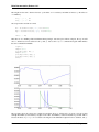
subplot(211)
raster_plot(M, title=’The CUBA network’, newfigure=False)
subplot(223)
plot(MV.times / ms, MV[0] / mV)
xlabel(’Time (ms)’)
ylabel(’V (mV)’)
subplot(224)
plot(Mge.times / ms, Mge[0] / mV)
plot(Mgi.times / ms, Mgi[0] / mV)
xlabel(’Time (ms)’)
ylabel(’ge and gi (mV)’)
legend((’ge’, ’gi’), ’upper right’)
show()
3.1. Tutorials
27
Brian Documentation, Release 1.2.1
3.2 Examples
These examples cover some basic topics in writing Brian scripts in Python. The complete source code for the examples
is available in the examples folder in the extras package.
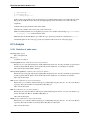
3.2.1 plasticity
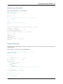
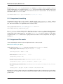
Example: short_term_plasticity (plasticity)
Example with short term plasticity model Neurons with regular inputs and depressing synapses
from brian import *
tau_e = 3 * ms
taum = 10 * ms
A_SE = 250 * pA
Rm = 100 * Mohm
N = 10
eqs = ’’’
dx/dt=rate : 1
rate : Hz
’’’
input = NeuronGroup(N, model=eqs, threshold=1., reset=0)
input.rate = linspace(5 * Hz, 30 * Hz, N)
eqs_neuron = ’’’
dv/dt=(Rm*i-v)/taum:volt
di/dt=-i/tau_e:amp
’’’
neuron = NeuronGroup(N, model=eqs_neuron)
C = Connection(input, neuron, ’i’)
C.connect_one_to_one(weight=A_SE)
stp = STP(C, taud=1 * ms, tauf=100 * ms, U=.1) # facilitation
#stp=STP(C,taud=100*ms,tauf=10*ms,U=.6) # depression
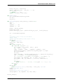
trace = StateMonitor(neuron, ’v’, record=[0, N - 1])
run(1000 * ms)
subplot(211)
plot(trace.times / ms, trace[0] / mV)
title(’Vm’)
subplot(212)
plot(trace.times / ms, trace[N - 1] / mV)
title(’Vm’)
show()
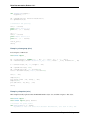
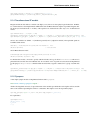
Example: short_term_plasticity2 (plasticity)
Network (CUBA) with short-term synaptic plasticity for excitatory synapses (Depressing at long timescales, facilitating at short timescales)
28
Chapter 3. Getting started
Brian Documentation, Release 1.2.1
from brian import *
from time import time
eqs = ’’’
dv/dt = (ge+gi-(v+49*mV))/(20*ms) : volt
dge/dt = -ge/(5*ms) : volt
dgi/dt = -gi/(10*ms) : volt
’’’
P = NeuronGroup(4000, model=eqs, threshold= -50 * mV, reset= -60 * mV)
P.v = -60 * mV + rand(4000) * 10 * mV
Pe = P.subgroup(3200)
Pi = P.subgroup(800)
Ce = Connection(Pe, P, ’ge’, weight=1.62 * mV, sparseness=.02)
Ci = Connection(Pi, P, ’gi’, weight= -9 * mV, sparseness=.02)
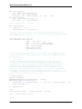
stp = STP(Ce, taud=200 * ms, tauf=20 * ms, U=.2)
M = SpikeMonitor(P)
rate = PopulationRateMonitor(P)
t1 = time()
run(1 * second)
t2 = time()
print "Simulation time:", t2 - t1, "s"
print M.nspikes, "spikes"
subplot(211)
raster_plot(M)
subplot(212)
plot(rate.times / ms, rate.smooth_rate(5 * ms))
show()
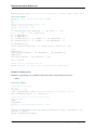
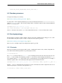
Example: STDP1 (plasticity)
Spike-timing dependent plasticity Adapted from Song, Miller and Abbott (2000) and Song and Abbott (2001)
This simulation takes a long time!
from brian import *
from time import time
N = 1000
taum = 10 * ms
tau_pre = 20 * ms
tau_post = tau_pre
Ee = 0 * mV
vt = -54 * mV
vr = -60 * mV
El = -74 * mV
taue = 5 * ms
F = 15 * Hz
gmax = .01
dA_pre = .01
dA_post = -dA_pre * tau_pre / tau_post * 1.05
eqs_neurons = ’’’
dv/dt=(ge*(Ee-vr)+El-v)/taum : volt
dge/dt=-ge/taue : 1
’’’
3.2. Examples
# the synaptic current is linearized
29
Brian Documentation, Release 1.2.1
input = PoissonGroup(N, rates=F)
neurons = NeuronGroup(1, model=eqs_neurons, threshold=vt, reset=vr)
synapses = Connection(input, neurons, ’ge’, weight=rand(len(input), len(neurons)) * gmax)
neurons.v = vr
#stdp=ExponentialSTDP(synapses,tau_pre,tau_post,dA_pre,dA_post,wmax=gmax)
## Explicit STDP rule
eqs_stdp = ’’’
dA_pre/dt=-A_pre/tau_pre : 1
dA_post/dt=-A_post/tau_post : 1
’’’
dA_post *= gmax
dA_pre *= gmax
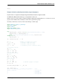
stdp = STDP(synapses, eqs=eqs_stdp, pre=’A_pre+=dA_pre;w+=A_post’,
post=’A_post+=dA_post;w+=A_pre’, wmax=gmax)
rate = PopulationRateMonitor(neurons)
start_time = time()
run(100 * second, report=’text’)
print "Simulation time:", time() - start_time
subplot(311)
plot(rate.times / second, rate.smooth_rate(100 * ms))
subplot(312)
plot(synapses.W.todense() / gmax, ’.’)
subplot(313)
hist(synapses.W.todense() / gmax, 20)
show()
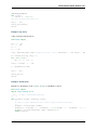
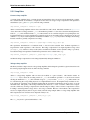
Example: STDP2 (plasticity)
Spike-timing dependent plasticity Adapted from Song, Miller and Abbott (2000), Song and Abbott (2001) and van
Rossum et al (2000).
This simulation takes a long time!
from brian import *
from time import time
N = 1000
taum = 10 * ms
tau_pre = 20 * ms
tau_post = tau_pre
Ee = 0 * mV
vt = -54 * mV
vr = -60 * mV
El = -74 * mV
taue = 5 * ms
gmax = 0.01
F = 15 * Hz
dA_pre = .01
dA_post = -dA_pre * tau_pre / tau_post * 2.5
eqs_neurons = ’’’
dv/dt=(ge*(Ee-vr)+El-v)/taum : volt
30
# the synaptic current is linearized
Chapter 3. Getting started
Brian Documentation, Release 1.2.1
dge/dt=-ge/taue : 1
’’’
input = PoissonGroup(N, rates=F)
neurons = NeuronGroup(1, model=eqs_neurons, threshold=vt, reset=vr)
synapses = Connection(input, neurons, ’ge’, weight=rand(len(input), len(neurons)) * gmax,
structure=’dense’)
neurons.v = vr
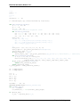
stdp = ExponentialSTDP(synapses, tau_pre, tau_post, dA_pre, dA_post, wmax=gmax, update=’mixed’)
rate = PopulationRateMonitor(neurons)
start_time = time()
run(100 * second, report=’text’)
print "Simulation time:", time() - start_time
subplot(311)
plot(rate.times / second, rate.smooth_rate(100 * ms))
subplot(312)
plot(synapses.W.todense() / gmax, ’.’)
subplot(313)
hist(synapses.W.todense() / gmax, 20)
show()
3.2.2 multiprocessing
Example: multiple_runs_simple (multiprocessing)
Example of using Python multiprocessing module to distribute simulations over multiple processors.
The general procedure for using multiprocessing is to define and run a network inside a function, and then use multiprocessing.Pool.map to call the function with multiple parameter values. Note that on Windows, any code that should
only run once should be placed inside an if __name__==’__main__’ block.
from brian import *
import multiprocessing
# This is the function that we want to compute for various different parameters
def how_many_spikes(excitatory_weight):
# These two lines reset the clock to 0 and clear any remaining data so that
# memory use doesn’t build up over multiple runs.
reinit_default_clock()
clear(True)
eqs = ’’’
dv/dt = (ge+gi-(v+49*mV))/(20*ms) : volt
dge/dt = -ge/(5*ms) : volt
dgi/dt = -gi/(10*ms) : volt
’’’
P = NeuronGroup(4000, eqs, threshold= -50 * mV, reset= -60 * mV)
P.v = -60 * mV + 10 * mV * rand(len(P))
Pe = P.subgroup(3200)
Pi = P.subgroup(800)
Ce = Connection(Pe, P, ’ge’)
Ci = Connection(Pi, P, ’gi’)
Ce.connect_random(Pe, P, 0.02, weight=excitatory_weight)
3.2. Examples
31
Brian Documentation, Release 1.2.1
Ci.connect_random(Pi, P, 0.02, weight= -9 * mV)
M = SpikeMonitor(P)
run(100 * ms)
return M.nspikes
if __name__ == ’__main__’:
# Note that on Windows platforms, all code that is executed rather than
# just defining functions and classes has to be in the if __name__==’__main__’
# block, otherwise it will be executed by each process that starts. This
# isn’t a problem on Linux.
pool = multiprocessing.Pool() # uses num_cpu processes by default
weights = linspace(0, 3.5, 100) * mV
args = [w * volt for w in weights]
results = pool.map(how_many_spikes, args) # launches multiple processes
plot(weights, results, ’.’)
show()
Example: multiple_runs_with_gui (multiprocessing)
A complicated example of using multiprocessing for multiple runs of a simulation with different parameters, using a
GUI to monitor and control the runs.
This example features:
• An indefinite number of runs, with a set of parameters for each run generated at random for each run.
• A plot of the output of all the runs updated as soon as each run is completed.
• A GUI showing how long each process has been running for and how long until it completes, and with a button
allowing you to terminate the runs.
A simpler example is in examples/multiprocessing/multiple_runs_simple.py.
# We use Tk as the backend for the GUI and matplotlib so as to avoid any
# threading conflicts
import matplotlib
matplotlib.use(’TkAgg’)
from brian import *
import Tkinter, time, multiprocessing, os
from brian.utils.progressreporting import make_text_report
from Queue import Empty as QueueEmpty
class SimulationController(Tkinter.Tk):
’’’
GUI, uses Tkinter and features a progress bar for each process, and a callback
function for when the terminate button is clicked.
’’’
def __init__(self, processes, terminator, width=600):
Tkinter.Tk.__init__(self, None)
self.parent = None
self.grid()
button = Tkinter.Button(self, text=’Terminate simulation’,
command=terminator)
button.grid(column=0, row=0)
self.pb_width = width
self.progressbars = []
32
Chapter 3. Getting started
Brian Documentation, Release 1.2.1
for i in xrange(processes):
can = Tkinter.Canvas(self, width=width, height=30)
can.grid(column=0, row=1 + i)
can.create_rectangle(0, 0, width, 30, fill=’#aaaaaa’)
r = can.create_rectangle(0, 0, 0, 30, fill=’#ffaaaa’, width=0)
t = can.create_text(width / 2, 15, text=’’)
self.progressbars.append((can, r, t))
self.results_text = Tkinter.Label(self, text=’Computed 0 results, time taken: 0s’)
self.results_text.grid(column=0, row=processes + 1)
self.title(’Simulation control’)
def update_results(self, elapsed, complete):
’’’
Method to update the total number of results computed and the amount of time taken.
’’’
self.results_text.config(text=’Computed ’ + str(complete) + ’, time taken: ’ + str(int(elapse
self.update()
def update_process(self, i, elapsed, complete, msg):
’’’
Method to update the status of a given process.
’’’
can, r, t = self.progressbars[i]
can.itemconfigure(t, text=’Process ’ + str(i) + ’: ’ + make_text_report(elapsed, complete) +
can.coords(r, 0, 0, int(self.pb_width * complete), 30)
self.update()
def sim_mainloop(pool, results, message_queue):
’’’
Monitors results of a simulation as they arrive
pool is the multiprocessing.Pool that the processes are running in,
results is the AsyncResult object returned by Pool.imap_unordered which
returns simulation results asynchronously as and when they are ready,
and message_queue is a multiprocessing.Queue used to communicate between
child processes and the server process. In this case, we use this Queue to
send messages about the percent complete and time elapsed for each run.
’’’
# We use this to enumerate the processes, mapping their process IDs to an int
# in the range 0:num_processes.
pid_to_id = dict((pid, i) for i, pid in enumerate([p.pid for p in pool._pool]))
num_processes = len(pid_to_id)
start = time.time()
stoprunningsim = [False]
# This function terminates all the pool’s child processes, it is used as
# the callback function called when the terminate button on the GUI is clicked.
def terminate_sim():
pool.terminate()
stoprunningsim[0] = True
controller = SimulationController(num_processes, terminate_sim)
for i in range(num_processes):
controller.update_process(i, 0, 0, ’no info yet’)
i = 0
while True:
try:
# If there is a new result (the 0.1 means wait 0.1 seconds for a
# result before giving up) then this try clause will execute, otherwise
# a TimeoutError will occur and the except clause afterwards will
3.2. Examples
33
Brian Documentation, Release 1.2.1
# execute.
weight, numspikes = results.next(0.1)
# if we reach here, we have a result to plot, so we plot it and
# update the GUI
plot_result(weight, numspikes)
i = i + 1
controller.update_results(time.time() - start, i)
except multiprocessing.TimeoutError:
# if we’re still waiting for a new result, we can process events in
# the message_queue and update the GUI if there are any.
while not message_queue.empty():
try:
# messages here are of the form: (pid, elapsed, complete)
# where pid is the process ID of the child process, elapsed
# is the amount of time elapsed, and complete is the
# fraction of the run completed. See function how_many_spikes
# to see where these messages come from.
pid, elapsed, complete = message_queue.get_nowait()
controller.update_process(pid_to_id[pid], elapsed, complete, ’’)
except QueueEmpty:
break
controller.update()
if stoprunningsim[0]:
print ’Terminated simulation processes’
break
controller.destroy()
def plot_result(weight, numspikes):
plot([weight], [numspikes], ’.’, color=(0, 0, 0.5))
axis(’tight’)
draw() # this forces matplotlib to redraw
# Note that how_many_spikes only takes one argument, which is a tuple of
# its actual arguments. The reason for this is that Pool.imap_unordered can only
# pass a single argument to the function its applied to, but that argument can
# be a tuple...
def how_many_spikes((excitatory_weight, message_queue)):
reinit_default_clock()
clear(True)
eqs = ’’’
dv/dt = (ge+gi-(v+49*mV))/(20*ms) : volt
dge/dt = -ge/(5*ms) : volt
dgi/dt = -gi/(10*ms) : volt
’’’
P = NeuronGroup(4000, eqs, threshold= -50 * mV, reset= -60 * mV)
P.v = -60 * mV + 10 * mV * rand(len(P))
Pe = P.subgroup(3200)
Pi = P.subgroup(800)
Ce = Connection(Pe, P, ’ge’)
Ci = Connection(Pi, P, ’gi’)
Ce.connect_random(Pe, P, 0.02, weight=excitatory_weight)
Ci.connect_random(Pi, P, 0.02, weight= -9 * mV)
M = SpikeMonitor(P)
# This reporter function is called every second, and it sends a message to
# the server process updating the status of the current run.
def reporter(elapsed, complete):
34
Chapter 3. Getting started
Brian Documentation, Release 1.2.1
message_queue.put((os.getpid(), elapsed, complete))
run(4000 * ms, report=reporter, report_period=1 * second)
return (excitatory_weight, M.nspikes)
if __name__ == ’__main__’:
numprocesses = None # number of processes to use, set to None to have one per CPU
# We have to use a Queue from the Manager to send messages from client
# processes to the server process
manager = multiprocessing.Manager()
message_queue = manager.Queue()
pool = multiprocessing.Pool(processes=numprocesses)
# This generator function repeatedly generates random sets of parameters
# to pass to the how_many_spikes function
def args():
while True:
weight = rand()*3.5 * mV
yield (weight, message_queue)
# imap_unordered returns an AsyncResult object which returns results as
# and when they are ready, we pass this results object which is returned
# immediately to the sim_mainloop function which monitors this, updates the
# GUI and plots the results as they come in.
results = pool.imap_unordered(how_many_spikes, args())
ion() # this puts matplotlib into interactive mode to plot as we go
sim_mainloop(pool, results, message_queue)
3.2.3 modelfitting
Example: modelfitting (modelfitting)
Model fitting example. Fits an integrate-and-fire model to an in-vitro electrophysiological recording during one second.
from brian import loadtxt, ms, Equations
from brian.library.modelfitting import *
if __name__ == ’__main__’:
equations = Equations(’’’
dV/dt=(R*I-V)/tau : 1
I : 1
R : 1
tau : second
’’’)
optinfo = dict([])
optinfo[’Minterval’] = 10
input = loadtxt(’current.txt’)
spikes = loadtxt(’spikes.txt’)
results = modelfitting(model=equations, reset=0, threshold=1,
data=spikes,
input=input, dt=.1 * ms,
particles=1000, iterations=10, delta=2 * ms,
3.2. Examples
35
Brian Documentation, Release 1.2.1
use_gpu=False, max_cpu=4, max_gpu=1,
R=[1.0e9, 9.0e9], tau=[10 * ms, 40 * ms], optalg=GA, optinfo=optinfo
print_results(results)
Example: modelfitting2 (modelfitting)
A second example of the modelfitting toolbox.
if __name__ == ’__main__’:
from brian import *
from modelfitting import *
model = ’’’
dV/dt=(R*I-V)/tau : 1
I : 1
R : 1
tau : second
’’’
threshold = 1
reset = 0
input = loadtxt(’current.txt’)
spikes0 = loadtxt(’spikes.txt’)
spikes = []
for i in xrange(2):
spikes.extend([(i, spike * second + 5 * i * ms) for spike in spikes0])
results = modelfitting(model=model, reset=reset, threshold=threshold,
data=spikes,
input=input, dt=.1 * ms,
max_cpu=4,
particles=1000, iterations=3, delta=2 * ms,
R=[1.0e9, 8.0e9],
tau=[10 * ms, 40 * ms],
_delays=[-10 * ms, 10 * ms])
print_results(results)
3.2.4 misc
Example: adaptive (misc)
An adaptive neuron model
from brian import *
PG = PoissonGroup(1, 500 * Hz)
eqs = ’’’
dv/dt = (-w-v)/(10*ms) : volt # the membrane equation
dw/dt = -w/(30*ms) : volt # the adaptation current
’’’
# The adaptation variable increases with each spike
IF = NeuronGroup(1, model=eqs, threshold=20 * mV,
reset=’’’v = 0*mV
36
Chapter 3. Getting started
Brian Documentation, Release 1.2.1
w += 3*mV ’’’)
C = Connection(PG, IF, ’v’, weight=3 * mV)
MS = SpikeMonitor(PG, True)
Mv = StateMonitor(IF, ’v’, record=True)
Mw = StateMonitor(IF, ’w’, record=True)
run(100 * ms)
plot(Mv.times / ms, Mv[0] / mV)
plot(Mw.times / ms, Mw[0] / mV)
show()
Example: adaptive_threshold (misc)
A model with adaptive threshold (increases with each spike)
from brian import *
eqs = ’’’
dv/dt = -v/(10*ms) : volt
dvt/dt = (10*mV-vt)/(15*ms) : volt
’’’
reset = ’’’
v=0*mV
vt+=3*mV
’’’
IF = NeuronGroup(1, model=eqs, reset=reset, threshold=’v>vt’)
IF.rest()
PG = PoissonGroup(1, 500 * Hz)
C = Connection(PG, IF, ’v’, weight=3 * mV)
Mv = StateMonitor(IF, ’v’, record=True)
Mvt = StateMonitor(IF, ’vt’, record=True)
run(100 * ms)
plot(Mv.times / ms, Mv[0] / mV)
plot(Mvt.times / ms, Mvt[0] / mV)
show()
Example: cable (misc)
Dendrite with 100 compartments
from brian import *
from brian.compartments import *
from brian.library.ionic_currents import *
3.2. Examples
37
Brian Documentation, Release 1.2.1
length = 1 * mm
nseg = 100
dx = length / nseg
Cm = 1 * uF / cm ** 2
gl = 0.02 * msiemens / cm ** 2
diam = 1 * um
area = pi * diam * dx
El = 0 * mV
Ri = 100 * ohm * cm
ra = Ri * 4 / (pi * diam ** 2)
print "Time constant =", Cm / gl
print "Space constant =", .5 * (diam / (gl * Ri)) ** .5
segments = {}
for i in range(nseg):
segments[i] = MembraneEquation(Cm * area) + leak_current(gl * area, El)
segments[0] += Current(’I:nA’)
cable = Compartments(segments)
for i in range(nseg - 1):
cable.connect(i, i + 1, ra * dx)
neuron = NeuronGroup(1, model=cable)
#neuron.vm_0=10*mV
neuron.I_0 = .05 * nA
trace = []
for i in range(10):
trace.append(StateMonitor(neuron, ’vm_’ + str(10 * i), record=True))
run(200 * ms)
for i in range(10):
plot(trace[i].times / ms, trace[i][0] / mV)
show()
Example: COBA (misc)
This is a Brian script implementing a benchmark described in the following review paper:
Simulation of networks of spiking neurons: A review of tools and strategies (2007). Brette, Rudolph, Carnevale, Hines,
Beeman, Bower, Diesmann, Goodman, Harris, Zirpe, Natschlager, Pecevski, Ermentrout, Djurfeldt, Lansner, Rochel,
Vibert, Alvarez, Muller, Davison, El Boustani and Destexhe. Journal of Computational Neuroscience 23(3):349-98
Benchmark 1: random network of integrate-and-fire neurons with exponential synaptic conductances
Clock-driven implementation with Euler integration (no spike time interpolation)
R. Brette - Dec 2007
Brian is a simulator for spiking neural networks written in Python, developed by R. Brette and D. Goodman.
http://brian.di.ens.fr
38
Chapter 3. Getting started
Brian Documentation, Release 1.2.1
from brian import *
import time
# Time constants
taum = 20 * msecond
taue = 5 * msecond
taui = 10 * msecond
# Reversal potentials
Ee = (0. + 60.) * mvolt
Ei = (-80. + 60.) * mvolt
start_time = time.time()
eqs = Equations(’’’
dv/dt = (-v+ge*(Ee-v)+gi*(Ei-v))*(1./taum) : volt
dge/dt = -ge*(1./taue) : 1
dgi/dt = -gi*(1./taui) : 1
’’’)
# NB 1: conductances are in units of the leak conductance
# NB 2: multiplication is faster than division
P = NeuronGroup(4000, model=eqs, threshold=10 * mvolt, \
reset=0 * mvolt, refractory=5 * msecond,
order=1, compile=True)
Pe = P.subgroup(3200)
Pi = P.subgroup(800)
we = 6. / 10. # excitatory synaptic weight (voltage)
wi = 67. / 10. # inhibitory synaptic weight
Ce = Connection(Pe, P, ’ge’, weight=we, sparseness=0.02)
Ci = Connection(Pi, P, ’gi’, weight=wi, sparseness=0.02)
# Initialization
P.v = (randn(len(P)) * 5 - 5) * mvolt
P.ge = randn(len(P)) * 1.5 + 4
P.gi = randn(len(P)) * 12 + 20
# Record the number of spikes
Me = PopulationSpikeCounter(Pe)
Mi = PopulationSpikeCounter(Pi)
print "Network construction time:", time.time() - start_time, "seconds"
print "Simulation running..."
start_time = time.time()
run(1 * second)
duration = time.time() - start_time
print "Simulation time:", duration, "seconds"
print Me.nspikes, "excitatory spikes"
print Mi.nspikes, "inhibitory spikes"
Example: COBAHH (misc)
This is an implementation of a benchmark described in the following review paper:
Simulation of networks of spiking neurons: A review of tools and strategies (2006). Brette, Rudolph, Carnevale,
Hines, Beeman, Bower, Diesmann, Goodman, Harris, Zirpe, NatschlAger, Pecevski, Ermentrout, Djurfeldt, Lansner,
Rochel, Vibert, Alvarez, Muller, Davison, El Boustani and Destexhe. Journal of Computational Neuroscience
Benchmark 3: random network of HH neurons with exponential synaptic conductances
3.2. Examples
39
Brian Documentation, Release 1.2.1
Clock-driven implementation (no spike time interpolation)
1. Brette - Dec 2007
70s for dt=0.1 ms with exponential Euler
from brian import *
# Parameters
area = 20000 * umetre ** 2
Cm = (1 * ufarad * cm ** -2) * area
gl = (5e-5 * siemens * cm ** -2) * area
El = -60 * mV
EK = -90 * mV
ENa = 50 * mV
g_na = (100 * msiemens * cm ** -2) * area
g_kd = (30 * msiemens * cm ** -2) * area
VT = -63 * mV
# Time constants
taue = 5 * ms
taui = 10 * ms
# Reversal potentials
Ee = 0 * mV
Ei = -80 * mV
we = 6 * nS # excitatory synaptic weight (voltage)
wi = 67 * nS # inhibitory synaptic weight
# The model
eqs = Equations(’’’
dv/dt = (gl*(El-v)+ge*(Ee-v)+gi*(Ei-v)-\
g_na*(m*m*m)*h*(v-ENa)-\
g_kd*(n*n*n*n)*(v-EK))/Cm : volt
dm/dt = alpham*(1-m)-betam*m : 1
dn/dt = alphan*(1-n)-betan*n : 1
dh/dt = alphah*(1-h)-betah*h : 1
dge/dt = -ge*(1./taue) : siemens
dgi/dt = -gi*(1./taui) : siemens
alpham = 0.32*(mV**-1)*(13*mV-v+VT)/ \
(exp((13*mV-v+VT)/(4*mV))-1.)/ms : Hz
betam = 0.28*(mV**-1)*(v-VT-40*mV)/ \
(exp((v-VT-40*mV)/(5*mV))-1)/ms : Hz
alphah = 0.128*exp((17*mV-v+VT)/(18*mV))/ms : Hz
betah = 4./(1+exp((40*mV-v+VT)/(5*mV)))/ms : Hz
alphan = 0.032*(mV**-1)*(15*mV-v+VT)/ \
(exp((15*mV-v+VT)/(5*mV))-1.)/ms : Hz
betan = .5*exp((10*mV-v+VT)/(40*mV))/ms : Hz
’’’)
P = NeuronGroup(4000, model=eqs,
threshold=EmpiricalThreshold(threshold= -20 * mV,
refractory=3 * ms),
implicit=True, freeze=True)
Pe = P.subgroup(3200)
Pi = P.subgroup(800)
Ce = Connection(Pe, P, ’ge’, weight=we, sparseness=0.02)
Ci = Connection(Pi, P, ’gi’, weight=wi, sparseness=0.02)
# Initialization
P.v = El + (randn(len(P)) * 5 - 5) * mV
P.ge = (randn(len(P)) * 1.5 + 4) * 10. * nS
40
Chapter 3. Getting started
Brian Documentation, Release 1.2.1
P.gi = (randn(len(P)) * 12 + 20) * 10. * nS
# Record the number of spikes and a few traces
trace = StateMonitor(P, ’v’, record=[1, 10, 100])
run(1 * second)
plot(trace[1])
plot(trace[10])
plot(trace[100])
show()
Example: correlated_inputs (misc)
An example with correlated spike trains From: Brette, R. (2007). Generation of correlated spike trains.
from brian import *
input = HomogeneousCorrelatedSpikeTrains(1000, r=10 * Hz, c=0.1, tauc=10 * ms)
S = SpikeMonitor(input)
S2 = PopulationRateMonitor(input)
M = StateMonitor(input, ’rate’, record=0)
run(1000 * ms)
subplot(211)
raster_plot(S)
subplot(212)
plot(S2.times / ms, S2.smooth_rate(5 * ms))
plot(M.times / ms, M[0] / Hz)
show()
Example: CUBA (misc)
This is a Brian script implementing a benchmark described in the following review paper:
Simulation of networks of spiking neurons: A review of tools and strategies (2007). Brette, Rudolph, Carnevale, Hines,
Beeman, Bower, Diesmann, Goodman, Harris, Zirpe, Natschlager, Pecevski, Ermentrout, Djurfeldt, Lansner, Rochel,
Vibert, Alvarez, Muller, Davison, El Boustani and Destexhe. Journal of Computational Neuroscience 23(3):349-98
Benchmark 2: random network of integrate-and-fire neurons with exponential synaptic currents
Clock-driven implementation with exact subthreshold integration (but spike times are aligned to the grid)
R. Brette - Oct 2007
Brian is a simulator for spiking neural networks written in Python, developed by R. Brette and D. Goodman.
http://brian.di.ens.fr
from brian import *
import time
start_time = time.time()
taum = 20 * ms
taue = 5 * ms
3.2. Examples
41
Brian Documentation, Release 1.2.1
taui
Vt =
Vr =
El =
= 10 * ms
-50 * mV
-60 * mV
-49 * mV
eqs = Equations(’’’
dv/dt = (ge+gi-(v-El))/taum : volt
dge/dt = -ge/taue : volt
dgi/dt = -gi/taui : volt
’’’)
P = NeuronGroup(4000, model=eqs, threshold=Vt, reset=Vr, refractory=5 * ms)
P.v = Vr
P.ge = 0 * mV
P.gi = 0 * mV
Pe = P.subgroup(3200)
Pi = P.subgroup(800)
we = (60 * 0.27 / 10) * mV # excitatory
wi = (-20 * 4.5 / 10) * mV # inhibitory
Ce = Connection(Pe, P, ’ge’, weight=we,
Ci = Connection(Pi, P, ’gi’, weight=wi,
P.v = Vr + rand(len(P)) * (Vt - Vr)
synaptic weight (voltage)
synaptic weight
sparseness=0.02)
sparseness=0.02)
# Record the number of spikes
Me = PopulationSpikeCounter(Pe)
Mi = PopulationSpikeCounter(Pi)
# A population rate monitor
M = PopulationRateMonitor(P)
print "Network construction time:", time.time() - start_time, "seconds"
print len(P), "neurons in the network"
print "Simulation running..."
run(1 * msecond)
start_time = time.time()
run(1 * second)
duration = time.time() - start_time
print "Simulation time:", duration, "seconds"
print Me.nspikes, "excitatory spikes"
print Mi.nspikes, "inhibitory spikes"
plot(M.times / ms, M.smooth_rate(2 * ms, ’gaussian’))
show()
Example: current_clamp (misc)
An example of single-electrode current clamp recording with bridge compensation (using the electrophysiology library).
from brian import *
from brian.library.electrophysiology import *
taum = 20 * ms
# membrane time constant
gl = 1. / (50 * Mohm)
# leak conductance
Cm = taum * gl
# membrane capacitance
42
Chapter 3. Getting started
Brian Documentation, Release 1.2.1
Re = 50 * Mohm
Ce = 0.5 * ms / Re
# electrode resistance
# electrode capacitance
eqs = Equations(’’’
dvm/dt=(-gl*vm+i_inj)/Cm : volt
Rbridge:ohm # bridge resistance
I:amp # command current
’’’)
eqs += current_clamp(i_cmd=’I’, Re=Re, Ce=Ce, bridge=’Rbridge’)
setup = NeuronGroup(1, model=eqs)
soma = StateMonitor(setup, ’vm’, record=True)
recording = StateMonitor(setup, ’v_rec’, record=True)
# No compensation
run(50 * ms)
setup.I = .5 * nA
run(100 * ms)
setup.I = 0 * nA
run(50 * ms)
# Full compensation
setup.Rbridge = Re
run(50 * ms)
setup.I = .5 * nA
run(100 * ms)
setup.I = 0 * nA
run(50 * ms)
plot(recording.times / ms, recording[0] / mV, ’b’)
plot(soma.times / ms, soma[0] / mV, ’r’)
show()
Example: delays (misc)
Random network with external noise and transmission delays
from brian import *
tau = 10 * ms
sigma = 5 * mV
eqs = ’dv/dt = -v/tau+sigma*xi/tau**.5 : volt’
P = NeuronGroup(4000, model=eqs, threshold=10 * mV, reset=0 * mV, \
refractory=5 * ms)
P.v = -60 * mV
Pe = P.subgroup(3200)
Pi = P.subgroup(800)
C = Connection(P, P, ’v’, delay=2 * ms)
C.connect_random(Pe, P, 0.05, weight=.7 * mV)
C.connect_random(Pi, P, 0.05, weight= -2.8 * mV)
M = SpikeMonitor(P, True)
run(1 * second)
print ’Mean rate =’, M.nspikes / 4000. / second
raster_plot(M)
show()
3.2. Examples
43
Brian Documentation, Release 1.2.1
Example: expIF_network (misc)
A network of exponential IF models with synaptic conductances
from brian import *
from brian.library.IF import *
from brian.library.synapses import *
import time
C = 200 * pF
taum = 10 * msecond
gL = C / taum
EL = -70 * mV
VT = -55 * mV
DeltaT = 3 * mV
# Synapse parameters
Ee = 0 * mvolt
Ei = -80 * mvolt
taue = 5 * msecond
taui = 10 * msecond
eqs = exp_IF(C, gL, EL, VT, DeltaT)
# Two different ways of adding synaptic currents:
eqs += Current(’’’
Ie=ge*(Ee-vm) : amp
dge/dt=-ge/taue : siemens
’’’)
eqs += exp_conductance(’gi’, Ei, taui) # from library.synapses
P = NeuronGroup(4000, model=eqs, threshold= -20 * mvolt, reset=EL, refractory=2 * ms)
Pe = P.subgroup(3200)
Pi = P.subgroup(800)
we = 1.5 * nS # excitatory synaptic weight
wi = 2.5 * we # inhibitory synaptic weight
Ce = Connection(Pe, P, ’ge’, weight=we, sparseness=0.05)
Ci = Connection(Pi, P, ’gi’, weight=wi, sparseness=0.05)
# Initialization
P.vm = randn(len(P)) * 10 * mV - 70 * mV
P.ge = (randn(len(P)) * 2 + 5) * we
P.gi = (randn(len(P)) * 2 + 5) * wi
# Excitatory input to a subset of excitatory and inhibitory neurons
# Excitatory neurons are excited for the first 200 ms
# Inhibitory neurons are excited for the first 100 ms
input_layer1 = Pe.subgroup(200)
input_layer2 = Pi.subgroup(200)
input1 = PoissonGroup(200, rates=lambda t: (t < 200 * ms and 2000 * Hz) or 0 * Hz)
input2 = PoissonGroup(200, rates=lambda t: (t < 100 * ms and 2000 * Hz) or 0 * Hz)
input_co1 = IdentityConnection(input1, input_layer1, ’ge’, weight=we)
input_co2 = IdentityConnection(input2, input_layer2, ’ge’, weight=we)
# Record the number of spikes
M = SpikeMonitor(P)
print "Simulation running..."
start_time = time.time()
run(500 * ms)
44
Chapter 3. Getting started
Brian Documentation, Release 1.2.1
duration = time.time() - start_time
print "Simulation time:", duration, "seconds"
print M.nspikes / 4000., "spikes per neuron"
raster_plot(M)
show()
Example: gap_junctions (misc)
Network of noisy IF neurons with gap junctions
from brian import *
N = 300
v0 = 5 * mV
tau = 20 * ms
sigma = 5 * mV
vt = 10 * mV
vr = 0 * mV
g_gap = 1. / N
beta = 60 * mV * 2 * ms
delta = vt - vr
eqs = ’’’
dv/dt=(v0-v)/tau+g_gap*(u-N*v)/tau : volt
du/dt=(N*v0-u)/tau : volt # input from other neurons
’’’
def myreset(P, spikes):
P.v[spikes] = vr # reset
P.v += g_gap * beta * len(spikes) # spike effect
P.u -= delta * len(spikes)
group = NeuronGroup(N, model=eqs, threshold=vt, reset=myreset)
@network_operation
def noise(cl):
x = randn(N) * sigma * (cl.dt / tau) ** .5
group.v += x
group.u += sum(x)
trace = StateMonitor(group, ’v’, record=[0, 1])
spikes = SpikeMonitor(group)
rate = PopulationRateMonitor(group)
run(1 * second)
subplot(311)
raster_plot(spikes)
subplot(312)
plot(trace.times / ms, trace[0] / mV)
plot(trace.times / ms, trace[1] / mV)
subplot(313)
plot(rate.times / ms, rate.smooth_rate(5 * ms) / Hz)
show()
3.2. Examples
45
Brian Documentation, Release 1.2.1
Example: heterogeneous_delays (misc)
Script demonstrating use of a Connection with homogenenous delays
The network consists of a ‘starter’ neuron which fires a single spike at time t=0, connected to 100 leaky integrate and
fire neurons with different delays for each target neuron, with the delays forming a quadratic curve centred at neuron
50. The longest delay is 10ms, and the network is run for 40ms. At the end, the delays are plotted above a colour plot
of the membrane potential of each of the target neurons as a function of time (demonstrating the delays).
from brian import *
# Starter neuron, threshold is below 0 so it fires immediately, reset is below
# threshold so it fires only once.
G = NeuronGroup(1, model=’V:1’, threshold= -1.0, reset= -2.0)
# 100 LIF neurons, no reset or threshold so they will not spike
H = NeuronGroup(100, model=’dV/dt=-V/(10*ms):volt’)
# Connection with delays, here the delays are specified as a function of (i,j)
# giving the delay from neuron i to neuron j. In this case there is only one
# presynaptic neuron so i will be 0.
C = Connection(G, H, weight=5 * mV, max_delay=10 * ms,
delay=lambda i, j:10 * ms * (j / 50. - 1) ** 2)
M = StateMonitor(H, ’V’, record=True)
run(40 * ms)
subplot(211)
# These are the delays from neuron 0 to neuron i in ms
plot([C.delay[0, i] / ms for i in range(100)])
ylabel(’Delay (ms)’)
title(’Delays’)
subplot(212)
# M.values is an array of all the recorded values, here transposed to make
# it fit with the plot above.
imshow(M.values.T, aspect=’auto’, extent=(0, 100, 40, 0))
xlabel(’Neuron number’)
ylabel(’Time (ms)’)
title(’Potential’)
show()
Example: HodgkinHuxley (misc)
Hodgkin-Huxley model Assuming area 1*cm**2
#import brian_no_units
from brian import *
from brian.library.ionic_currents import *
#c=Clock(dt=.01*ms) # more precise
El = 10.6 * mV
EK = -12 * mV
ENa = 120 * mV
eqs = MembraneEquation(1 * uF) + leak_current(.3 * msiemens, El)
eqs += K_current_HH(36 * msiemens, EK) + Na_current_HH(120 * msiemens, ENa)
eqs += Current(’I:amp’)
neuron = NeuronGroup(1, eqs, implicit=True, freeze=True)
trace = StateMonitor(neuron, ’vm’, record=True)
46
Chapter 3. Getting started
Brian Documentation, Release 1.2.1
run(100 * ms)
neuron.I = 10 * uA
run(100 * ms)
plot(trace.times / ms, trace[0] / mV)
show()
Example: I-F_curve (misc)
Input-Frequency curve of a neuron (cortical RS type) Network: 1000 unconnected integrate-and-fire neurons (BretteGerstner) with an input parameter I. The input is set differently for each neuron. Spikes are sent to a ‘neuron’ group
with the same size and variable n, which has the role of a spike counter.
from brian import *
from brian.library.IF import *
N = 1000
eqs = Brette_Gerstner() + Current(’I:amp’)
print eqs
group = NeuronGroup(N, model=eqs, threshold= -20 * mV, reset=AdaptiveReset())
group.vm = -70 * mV
group.I = linspace(0 * nA, 1 * nA, N)
counter = NeuronGroup(N, model=’n:1’)
C = IdentityConnection(group, counter, ’n’)
i = N * 8 / 10
trace = StateMonitor(group, ’vm’, record=i)
duration = 5 * second
run(duration)
subplot(211)
plot(group.I / nA, counter.n / duration)
xlabel(’I (nA)’)
ylabel(’Firing rate (Hz)’)
subplot(212)
plot(trace.times / ms, trace[i] / mV)
xlabel(’Time (ms)’)
ylabel(’Vm (mV)’)
show()
Example: I-F_curve2 (misc)
Input-Frequency curve of a IF model Network: 1000 unconnected integrate-and-fire neurons (leaky IF) with an input
parameter v0. The input is set differently for each neuron. Spikes are sent to a spike counter (counts the spikes emitted
by each neuron).
from brian import *
N = 1000
tau = 10 * ms
eqs = ’’’
dv/dt=(v0-v)/tau : volt
v0 : volt
’’’
3.2. Examples
47
Brian Documentation, Release 1.2.1
group = NeuronGroup(N, model=eqs, threshold=10 * mV, reset=0 * mV, refractory=5 * ms)
group.v = 0 * mV
group.v0 = linspace(0 * mV, 20 * mV, N)
counter = SpikeCounter(group)
duration = 5 * second
run(duration)
plot(group.v0 / mV, counter.count / duration)
show()
Example: if (misc)
A very simple example Brian script to show how to implement an integrate and fire model. In this example, we also
drive the single integrate and fire neuron with regularly spaced spikes from the SpikeGeneratorGroup.
from brian import *
tau = 10 * ms
Vr = -70 * mV
Vt = -55 * mV
G = NeuronGroup(1, model=’V:volt’, threshold=Vt, reset=Vr)
input = SpikeGeneratorGroup(1, [(0, t * ms) for t in linspace(10, 100, 25)])
C = Connection(input, G)
C[0, 0] = 2 * mV
M = StateMonitor(G, ’V’, record=True)
G.V = Vr
run(100 * ms)
plot(M.times / ms, M[0] / mV)
show()
Example: leaky_if (misc)
A very simple example Brian script to show how to implement a leaky integrate and fire model. In this example, we
also drive the single leaky integrate and fire neuron with regularly spaced spikes from the SpikeGeneratorGroup.
from brian import *
tau = 10 * ms
Vr = -70 * mV
Vt = -55 * mV
G = NeuronGroup(1, model=’dV/dt = -(V-Vr)/tau : volt’, threshold=Vt, reset=Vr)
spikes = linspace(10 * ms, 100 * ms, 25)
input = MultipleSpikeGeneratorGroup([spikes])
C = Connection(input, G)
C[0, 0] = 5 * mV
48
Chapter 3. Getting started
Brian Documentation, Release 1.2.1
M = StateMonitor(G, ’V’, record=True)
G.V = Vr
run(100 * ms)
plot(M.times / ms, M[0] / mV)
show()
Example: linked_var (misc)
Example showing linked_var(), connecting two different NeuronGroup variables. Here we show something
like a simplified haircell and auditory nerve fibre model where the hair cells and ANFs are implemented as two separate
NeuronGroup objects. The hair cells filter their inputs via a differential equation, and then emit graded amounts of
neurotransmitter (variable ‘y’) to the auditory nerve fibres input current (variable ‘I’).
from brian import *
N = 5
f = 50 * Hz
a_min = 1.0
a_max = 100.0
tau_haircell = 50 * ms
tau = 10 * ms
duration = 100 * ms
eqs_haircells = ’’’
input = a*sin(2*pi*f*t) : 1
x = clip(input, 0, Inf)**(1.0/3.0) : 1
a : 1
dy/dt = (x-y)/tau_haircell : 1
’’’
haircells = NeuronGroup(N, eqs_haircells)
haircells.a = linspace(a_min, a_max, N)
M_haircells = MultiStateMonitor(haircells, vars=(’input’, ’y’), record=True)
eqs_nervefibres = ’’’
dV/dt = (I-V)/tau : 1
I : 1
’’’
nervefibres = NeuronGroup(N, eqs_nervefibres, reset=0, threshold=1)
nervefibres.I = linked_var(haircells, ’y’)
M_nervefibres = MultiStateMonitor(nervefibres, record=True)
run(duration)
subplot(221)
M_haircells[’input’].plot()
ylabel(’haircell.input’)
subplot(222)
M_haircells[’y’].plot()
ylabel(’haircell.y’)
subplot(223)
M_nervefibres[’I’].plot()
ylabel(’nervefibres.I’)
subplot(224)
3.2. Examples
49
Brian Documentation, Release 1.2.1
M_nervefibres[’V’].plot()
ylabel(’nervefibres.V’)
show()
Example: minimalexample (misc)
Very short example program.
from brian import *
eqs = ’’’
dv/dt = (ge+gi-(v+49*mV))/(20*ms) : volt
dge/dt = -ge/(5*ms) : volt
dgi/dt = -gi/(10*ms) : volt
’’’
P = NeuronGroup(4000, model=eqs,
threshold= -50 * mV, reset= -60 * mV)
P.v = -60 * mV + 10 * mV * rand(len(P))
Pe = P.subgroup(3200)
Pi = P.subgroup(800)
Ce = Connection(Pe, P, ’ge’, weight=1.62 * mV, sparseness=0.02)
Ci = Connection(Pi, P, ’gi’, weight= -9 * mV, sparseness=0.02)
M = SpikeMonitor(P)
run(1 * second)
i = 0
while len(M[i]) <= 1:
i += 1
print "The firing rate of neuron", i, "is", firing_rate(M[i]) * Hz
print "The coefficient of variation neuron", i, "is", CV(M[i])
raster_plot(M)
show()
Example: mirollo_strogatz (misc)
Mirollo-Strogatz network
from brian import *
tau = 10 * ms
v0 = 11 * mV
N = 20
w = .1 * mV
group = NeuronGroup(N, model=’dv/dt=(v0-v)/tau : volt’, threshold=10 * mV, reset=0 * mV)
W = Connection(group, group, ’v’, weight=w)
group.v = rand(N) * 10 * mV
S = SpikeMonitor(group)
50
Chapter 3. Getting started
Brian Documentation, Release 1.2.1
run(300 * ms)
raster_plot(S)
show()
Example: multipleclocks (misc)
This example demonstrates using different clocks for different objects in the network. The clock simclock is the
clock used for the underlying simulation. The clock monclock is the clock used for monitoring the membrane
potential. This monitoring takes place less frequently than the simulation update step to save time and memory.
Finally, the clock inputclock controls when the external ‘current’ Iext should be updated. In this case, we
update it infrequently so we can see the effect on the network.
This example also demonstrates the @network_operation decorator. A function with this decorator will be run as part
of the network update step, in sync with the clock provided (or the default one if none is provided).
from brian import *
# define the three clocks
simclock = Clock(dt=0.1 * ms)
monclock = Clock(dt=0.3 * ms)
inputclock = Clock(dt=100 * ms)
# simple leaky I&F model with external ’current’ Iext as a parameter
tau = 10 * ms
eqs = ’’’
dV/dt = (-V+Iext)/tau : volt
Iext: volt
’’’
# A single leaky I&F neuron with simclock as its clock
G = NeuronGroup(1, model=eqs, reset=0 * mV, threshold=10 * mV, clock=simclock)
G.V = 5 * mV
# This function will be run in sync with inputclock i.e. every 100 ms
@network_operation(clock=inputclock)
def update_Iext():
G.Iext = rand(len(G)) * 20 * mV
# V is monitored in sync with monclock
MV = StateMonitor(G, ’V’, record=0, clock=monclock)
# run and plot
run(1000 * ms)
plot(MV.times / ms, MV[0] / mV)
show()
# You should see 10 different regions, sometimes Iext will be above threshold
# in which case you will see regular spiking at different rates, and sometimes
# it will be below threshold in which case you’ll see exponential decay to that
# value
Example: named_threshold (misc)
Example with named threshold and reset variables
from brian import *
eqs = ’’’
dge/dt = -ge/(5*ms) : volt
dgi/dt = -gi/(10*ms) : volt
dx/dt = (ge+gi-(x+49*mV))/(20*ms) : volt
3.2. Examples
51
Brian Documentation, Release 1.2.1
’’’
P = NeuronGroup(4000, model=eqs, threshold=’x>-50*mV’, \
reset=Refractoriness(-60 * mV, 5 * ms, state=’x’))
#P=NeuronGroup(4000,model=eqs,threshold=Threshold(-50*mV,state=’x’),\
#
reset=Reset(-60*mV,state=’x’)) # without refractoriness
P.x = -60 * mV
Pe = P.subgroup(3200)
Pi = P.subgroup(800)
Ce = Connection(Pe, P, ’ge’, weight=1.62 * mV, sparseness=0.02)
Ci = Connection(Pi, P, ’gi’, weight= -9 * mV, sparseness=0.02)
M = SpikeMonitor(P)
run(1 * second)
raster_plot(M)
show()
Example: noisy_ring (misc)
Integrate-and-fire neurons with noise
from brian import *
tau = 10 * ms
sigma = .5
N = 100
J = -1
mu = 2
eqs = """
dv/dt=mu/tau+sigma/tau**.5*xi : 1
"""
group = NeuronGroup(N, model=eqs, threshold=1, reset=0)
C = Connection(group, group, ’v’)
for i in range(N):
C[i, (i + 1) % N] = J
#C.connect_full(group,group,weight=J)
#for i in range(N):
#
C[i,i]=0
S = SpikeMonitor(group)
trace = StateMonitor(group, ’v’, record=True)
run(500 * ms)
i, t = S.spikes[-1]
subplot(211)
raster_plot(S)
subplot(212)
plot(trace.times / ms, trace[0])
show()
52
Chapter 3. Getting started
Brian Documentation, Release 1.2.1
Example: phase_locking (misc)
Phase locking of IF neurons to a periodic input
from brian import *
tau
N =
b =
f =
= 20 * ms
100
1.2 # constant current mean, the modulation varies
10 * Hz
eqs = ’’’
dv/dt=(-v+a*sin(2*pi*f*t)+b)/tau : 1
a : 1
’’’
neurons = NeuronGroup(N, model=eqs, threshold=1, reset=0)
neurons.v = rand(N)
neurons.a = linspace(.05, 0.75, N)
S = SpikeMonitor(neurons)
trace = StateMonitor(neurons, ’v’, record=50)
run(1000 * ms)
subplot(211)
raster_plot(S)
subplot(212)
plot(trace.times / ms, trace[50])
show()
Example: poisson (misc)
This example demonstrates the PoissonGroup object. Here we have used a custom function to generate different rates
at different times.
This example also demonstrates a custom SpikeMonitor.
#import brian_no_units # uncomment to run faster
from brian import *
# Rates
r1 = arange(101, 201) * 0.1 * Hz
r2 = arange(1, 101) * 0.1 * Hz
def myrates(t):
if t < 10 * second:
return r1
else:
return r2
# More compact: myrates=lambda t: (t<10*second and r1) or r2
# Neuron group
P = PoissonGroup(100, myrates)
# Calculation of rates
ns = zeros(len(P))
3.2. Examples
53
Brian Documentation, Release 1.2.1
def ratemonitor(spikes):
ns[spikes] += 1
Mf = SpikeMonitor(P, function=ratemonitor)
M = SpikeMonitor(P)
# Simulation and plotting
run(10 * second)
print "Rates after 10s:"
print ns / (10 * second)
ns[:] = 0
run(10 * second)
print "Rates after 20s:"
print ns / (10 * second)
raster_plot()
show()
Example: poissongroup (misc)
Poisson input to an IF model
from brian import *
PG = PoissonGroup(1, lambda t:200 * Hz * (1 + cos(2 * pi * t * 50 * Hz)))
IF = NeuronGroup(1, model=’dv/dt=-v/(10*ms) : volt’, reset=0 * volt, threshold=10 * mV)
C = Connection(PG, IF, ’v’, weight=3 * mV)
MS = SpikeMonitor(PG, True)
Mv = StateMonitor(IF, ’v’, record=True)
rates = StateMonitor(PG, ’rate’, record=True)
run(100 * ms)
subplot(211)
plot(rates.times / ms, rates[0] / Hz)
subplot(212)
plot(Mv.times / ms, Mv[0] / mV)
show()
Example: pulsepacket (misc)
This example basically replicates what the Brian PulsePacket object does, and then compares to that object.
from brian import *
from random import gauss, shuffle
# Generator for pulse packet
def pulse_packet(t, n, sigma):
# generate a list of n times with Gaussian distribution, sort them in time, and
54
Chapter 3. Getting started
Brian Documentation, Release 1.2.1
# then randomly assign the neuron numbers to them
times = [gauss(t, sigma) for i in range(n)]
times.sort()
neuron = range(n)
shuffle(neuron)
return zip(neuron, times) # returns a list of pairs (i,t)
G1 = SpikeGeneratorGroup(1000, pulse_packet(50 * ms, 1000, 5 * ms))
M1 = SpikeMonitor(G1)
PRM1 = PopulationRateMonitor(G1, bin=1 * ms)
G2 = PulsePacket(50 * ms, 1000, 5 * ms)
M2 = SpikeMonitor(G2)
PRM2 = PopulationRateMonitor(G2, bin=1 * ms)
run(100 * ms)
subplot(221)
raster_plot(M1)
subplot(223)
plot(PRM1.rate)
subplot(222)
raster_plot(M2)
subplot(224)
plot(PRM2.rate)
show()
Example: rate_model (misc)
A rate model
from brian import *
N = 50000
tau = 20 * ms
I = 10 * Hz
eqs = ’’’
dv/dt=(I-v)/tau : Hz # note the unit here: this is the output rate
’’’
group = NeuronGroup(N, eqs, threshold=PoissonThreshold())
S = PopulationRateMonitor(group, bin=1 * ms)
run(100 * ms)
plot(S.rate)
show()
Example: realtime_plotting (misc)
Realtime plotting example
# These lines are necessary for interactive plotting when launching from the
# Eclipse IDE, they may not be necessary in every environment.
import matplotlib
3.2. Examples
55
Brian Documentation, Release 1.2.1
matplotlib.use(’WXAgg’) # You may need to experiment, try WXAgg, GTKAgg, QTAgg, TkAgg
from brian import *
###### Set up the standard CUBA example ######
N = 4000
eqs = ’’’
dv/dt = (ge+gi-(v+49*mV))/(20*ms) : volt
dge/dt = -ge/(5*ms) : volt
dgi/dt = -gi/(10*ms) : volt
’’’
P = NeuronGroup(N, eqs, threshold= -50 * mV, reset= -60 * mV)
P.v = -60 * mV + 10 * mV * rand(len(P))
Pe = P.subgroup(3200)
Pi = P.subgroup(800)
Ce = Connection(Pe, P, ’ge’, weight=1.62 * mV, sparseness=0.02)
Ci = Connection(Pi, P, ’gi’, weight= -9 * mV, sparseness=0.02)
M = SpikeMonitor(P)
trace = RecentStateMonitor(P, ’v’, record=range(5), duration=200 * ms)
ion()
subplot(211)
raster_plot(M, refresh=10 * ms, showlast=200 * ms, redraw=False)
subplot(212)
trace.plot(refresh=10 * ms, showlast=200 * ms)
run(1 * second)
ioff() # switch interactive mode off
show() # and wait for user to close the window before shutting down
Example: reliability (misc)
Reliability of spike timing. See e.g. Mainen & Sejnowski (1995) for experimental results in vitro.
1. Brette
from brian import *
# The common noisy input
N = 25
tau_input = 5 * ms
input = NeuronGroup(1, model=’dx/dt=-x/tau_input+(2./tau_input)**.5*xi:1’)
Min = StateMonitor(input, ’x’, record=True)
# The noisy neurons receiving the same input
tau = 10 * ms
sigma = .05
eqs_neurons = ’’’
dx/dt=(1.1+.5*I-x)/tau+sigma*(2./tau)**.5*xi:1
I : 1
’’’
neurons = NeuronGroup(N, model=eqs_neurons, threshold=1, reset=0, refractory=5 * ms)
neurons.x = rand(N)
spikes = SpikeMonitor(neurons)
56
Chapter 3. Getting started
Brian Documentation, Release 1.2.1
@network_operation
def inject():
neurons.I = input.x[0]
#neurons.I=linked_var(input,’x’)
run(500 * ms)
raster_plot(spikes)
show()
Example: ring (misc)
A ring of integrate-and-fire neurons.
from brian import *
tau = 10 * ms
v0 = 11 * mV
N = 20
w = 1 * mV
ring = NeuronGroup(N, model=’dv/dt=(v0-v)/tau : volt’, threshold=10 * mV, reset=0 * mV)
W = Connection(ring, ring, ’v’)
for i in range(N):
W[i, (i + 1) % N] = w
ring.v = rand(N) * 10 * mV
S = SpikeMonitor(ring)
run(300 * ms)
raster_plot(S)
show()
Example: stim2d (misc)
Example of a 2D stimulus, see the complete description at the Brian Cookbook.
from brian import *
import scipy.ndimage as im
__all__ = [’bar’, ’StimulusArrayGroup’]
def bar(width, height, thickness, angle):
’’’
An array of given dimensions with a bar of given thickness and angle
’’’
stimulus = zeros((width, height))
stimulus[:, int(height / 2. - thickness / 2.):int(height / 2. + thickness / 2.)] = 1.
stimulus = im.rotate(stimulus, angle, reshape=False)
return stimulus
3.2. Examples
57
Brian Documentation, Release 1.2.1
class StimulusArrayGroup(PoissonGroup):
’’’
A group of neurons which fire with a given stimulus at a given rate
The argument ‘‘stimulus‘‘ should be a 2D array with values between 0 and 1.
The point in the stimulus array at position (y,x) will correspond to the
neuron with index i=y*width+x. This neuron will fire Poisson spikes at
‘‘rate*stimulus[y,x]‘‘ Hz. The stimulus will start at time ‘‘onset‘‘
for ‘‘duration‘‘.
’’’
def __init__(self, stimulus, rate, onset, duration):
height, width = stimulus.shape
stim = stimulus.ravel()*rate
self.stimulus = stim
def stimfunc(t):
if onset < t < (onset + duration):
return stim
else:
return 0. * Hz
PoissonGroup.__init__(self, width * height, stimfunc)
if __name__ == ’__main__’:
import pylab
subplot(121)
stim = bar(100, 100, 10, 90) * 0.9 + 0.1
pylab.imshow(stim, origin=’lower’)
pylab.gray()
G = StimulusArrayGroup(stim, 50 * Hz, 100 * ms, 100 * ms)
M = SpikeMonitor(G)
run(300 * ms)
subplot(122)
raster_plot(M)
axis(xmin=0, xmax=300)
show()
Example: stopping (misc)
Network to demonstrate stopping a simulation during a run
Have a fully connected network of integrate and fire neurons with input fed by a group of Poisson neurons with a
steadily increasing rate, want to determine the point in time at which the network of integrate and fire neurons switches
from no firing to all neurons firing, so we have a network_operation called stop_condition that calls the stop() function
if the monitored network firing rate is above a minimum threshold.
from brian import *
clk = Clock()
Vr = 0 * mV
El = 0 * mV
Vt = 10 * mV
tau = 10 * ms
weight = 0.2 * mV
duration = 100 * msecond
max_input_rate = 10000 * Hz
num_input_neurons = 1000
58
Chapter 3. Getting started
Brian Documentation, Release 1.2.1
input_connection_p = 0.1
rate_per_neuron = max_input_rate / (num_input_neurons * input_connection_p)
P = PoissonGroup(num_input_neurons, lambda t: rate_per_neuron * (t / duration))
G = NeuronGroup(1000, model=’dV/dt=-(V-El)/tau : volt’, threshold=Vt, reset=Vr)
G.V = Vr + (Vt - Vr) * rand(len(G))
CPG = Connection(P, G, weight=weight, sparseness=input_connection_p)
CGG = Connection(G, G, weight=weight)
MP = PopulationRateMonitor(G, bin=1 * ms)
@network_operation
def stop_condition():
if MP.rate[-1] * Hz > 10 * Hz:
stop()
run(duration)
print "Reached population rate>10 Hz by time", clk.t, "+/- 1 ms."
Example: timed_array (misc)
An example of the TimedArray class used for applying input currents to neurons.
from brian import *
N = 5
duration = 100 * ms
Vr = -60 * mV
Vt = -50 * mV
tau = 10 * ms
Rmin = 1 * Mohm
Rmax = 10 * Mohm
freq = 50 * Hz
k = 10 * nA
eqs = ’’’
dV/dt = (-(V-Vr)+R*I)/tau : volt
R : ohm
I : amp
’’’
G = NeuronGroup(N, eqs, reset=’V=Vr’, threshold=’V>Vt’)
G.R = linspace(Rmin, Rmax, N)
t = linspace(0 * second, duration, int(duration / defaultclock.dt))
I = clip(k * sin(2 * pi * freq * t), 0, Inf)
G.I = TimedArray(I)
M = MultiStateMonitor(G, record=True)
run(duration)
3.2. Examples
59
Brian Documentation, Release 1.2.1
subplot(211)
M[’I’].plot()
ylabel(’I (amp)’)
subplot(212)
M[’V’].plot()
ylabel(’V (volt)’)
show()
Example: topographic_map (misc)
Topographic map - an example of complicated connections. Two layers of neurons. The first layer is connected
randomly to the second one in a topographical way. The second layer has random lateral connections.
from brian import *
N = 100
tau = 10 * ms
tau_e = 2 * ms # AMPA synapse
eqs = ’’’
dv/dt=(I-v)/tau : volt
dI/dt=-I/tau_e : volt
’’’
rates = zeros(N) * Hz
rates[N / 2 - 10:N / 2 + 10] = ones(20) * 30 * Hz
layer1 = PoissonGroup(N, rates=rates)
layer2 = NeuronGroup(N, model=eqs, threshold=10 * mV, reset=0 * mV)
topomap = lambda i, j:exp(-abs(i - j) * .1) * 3 * mV
feedforward = Connection(layer1, layer2, sparseness=.5, weight=topomap)
#feedforward[2,3]=1*mV
lateralmap = lambda i, j:exp(-abs(i - j) * .05) * 0.5 * mV
recurrent = Connection(layer2, layer2, sparseness=.5, weight=lateralmap)
spikes = SpikeMonitor(layer2)
run(1 * second)
subplot(211)
raster_plot(spikes)
subplot(223)
imshow(feedforward.W.todense(), interpolation=’nearest’, origin=’lower’)
title(’Feedforward connection strengths’)
subplot(224)
imshow(recurrent.W.todense(), interpolation=’nearest’, origin=’lower’)
title(’Recurrent connection strengths’)
show()
Example: topographic_map2 (misc)
Topographic map - an example of complicated connections. Two layers of neurons. The first layer is connected
randomly to the second one in a topographical way. The second layer has random lateral connections. Each neuron
has a position x[i].
60
Chapter 3. Getting started
Brian Documentation, Release 1.2.1
from brian import *
N = 100
tau = 10 * ms
tau_e = 2 * ms # AMPA synapse
eqs = ’’’
dv/dt=(I-v)/tau : volt
dI/dt=-I/tau_e : volt
’’’
rates = zeros(N) * Hz
rates[N / 2 - 10:N / 2 + 10] = ones(20) * 30 * Hz
layer1 = PoissonGroup(N, rates=rates)
layer1.x = linspace(0., 1., len(layer1)) # abstract position between 0 and 1
layer2 = NeuronGroup(N, model=eqs, threshold=10 * mV, reset=0 * mV)
layer2.x = linspace(0., 1., len(layer2))
# Generic connectivity function
topomap = lambda i, j, x, y, sigma: exp(-abs(x[i] - y[j]) / sigma)
feedforward = Connection(layer1, layer2, sparseness=.5,
weight=lambda i, j:topomap(i, j, layer1.x, layer2.x, .3) * 3 * mV)
recurrent = Connection(layer2, layer2, sparseness=.5,
weight=lambda i, j:topomap(i, j, layer1.x, layer2.x, .2) * .5 * mV)
spikes = SpikeMonitor(layer2)
run(1 * second)
subplot(211)
raster_plot(spikes)
subplot(223)
imshow(feedforward.W.todense(), interpolation=’nearest’, origin=’lower’)
title(’Feedforward connection strengths’)
subplot(224)
imshow(recurrent.W.todense(), interpolation=’nearest’, origin=’lower’)
title(’Recurrent connection strengths’)
show()
Example: transient_sync (misc)
Transient synchronisation in a population of noisy IF neurons with distance-dependent synaptic weights (organised as
a ring)
from brian import *
tau = 10 * ms
N = 100
v0 = 5 * mV
sigma = 4 * mV
group = NeuronGroup(N, model=’dv/dt=(v0-v)/tau + sigma*xi/tau**.5 : volt’, \
threshold=10 * mV, reset=0 * mV)
C = Connection(group, group, ’v’, weight=lambda i, j:.4 * mV * cos(2. * pi * (i - j) * 1. / N))
S = SpikeMonitor(group)
R = PopulationRateMonitor(group)
3.2. Examples
61
Brian Documentation, Release 1.2.1
group.v = rand(N) * 10 * mV
run(5000 * ms)
subplot(211)
raster_plot(S)
subplot(223)
imshow(C.W.todense(), interpolation=’nearest’)
title(’Synaptic connections’)
subplot(224)
plot(R.times / ms, R.smooth_rate(2 * ms, filter=’flat’))
title(’Firing rate’)
show()
Example: two_neurons (misc)
Two connected neurons with delays
from brian import *
tau = 10 * ms
w = -1 * mV
v0 = 11 * mV
neurons = NeuronGroup(2, model=’dv/dt=(v0-v)/tau : volt’, threshold=10 * mV, reset=0 * mV, \
max_delay=5 * ms)
neurons.v = rand(2) * 10 * mV
W = Connection(neurons, neurons, ’v’, delay=2 * ms)
W[0, 1] = w
W[1, 0] = w
S = StateMonitor(neurons, ’v’, record=True)
#mymonitor=SpikeMonitor(neurons[0])
mymonitor = PopulationSpikeCounter(neurons)
run(500 * ms)
plot(S.times / ms, S[0] / mV)
plot(S.times / ms, S[1] / mV)
show()
Example: using_classes (misc)
Example of using derived classes in Brian
Using a class derived from one of Brian’s classes can be a useful way of organising code in complicated simulations. A
class such as a NeuronGroup can itself create further NeuronGroup, Connection and NetworkOperation
objects. In order to have these objects included in the simulation, the derived class has to include them in its
contained_objects list (this tells Brian to add these to the Network when the derived class object is added
to the network).
from brian import *
class PoissonDrivenGroup(NeuronGroup):
’’’
This class is a group of leaky integrate-and-fire neurons driven by
external Poisson inputs. The class creates the Poisson inputs and
connects them to itself.
62
Chapter 3. Getting started
Brian Documentation, Release 1.2.1
’’’
def __init__(self, N, rate, weight):
tau = 10 * ms
eqs = ’’’
dV/dt = -V/tau : 1
’’’
# It’s essential to call the initialiser of the base class
super(PoissonDrivenGroup, self).__init__(N, eqs, reset=0, threshold=1)
self.poisson_group = PoissonGroup(N, rate)
self.conn = Connection(self.poisson_group, self, ’V’)
self.conn.connect_one_to_one(weight=weight)
self.contained_objects += [self.poisson_group,
self.conn]
G = PoissonDrivenGroup(100, 100 * Hz, .3)
M = SpikeMonitor(G)
M_pg = SpikeMonitor(G.poisson_group)
trace = StateMonitor(G, ’V’, record=0)
run(1 * second)
subplot(311)
raster_plot(M_pg)
title(’Input spikes’)
subplot(312)
raster_plot(M)
title(’Output spikes’)
subplot(313)
plot(trace.times, trace[0])
title(’Sample trace’)
show()
3.2.5 interface
Example: interface (interface)
Interface example Install cherrypy for this example Then run the script and go to http://localhost:8080 on your web
browser You can use cherrypy to write html interfaces to your code.
from brian import *
import cherrypy
import os.path
# The server is defined here
class MyInterface(object):
@cherrypy.expose
def index(self): # redirect to the html page we wrote
return ’<meta HTTP-EQUIV="Refresh" content="0;URL=index.html">’
@cherrypy.expose
def runscript(self, we="1.62", wi="-9", **kwd): # ’runscript’ is the script name
# we and wi are the names of form fields
we = float(we)
wi = float(wi)
# From minimalexample
3.2. Examples
63
Brian Documentation, Release 1.2.1
reinit_default_clock()
eqs = ’’’
dv/dt = (ge+gi-(v+49*mV))/(20*ms) : volt
dge/dt = -ge/(5*ms) : volt
dgi/dt = -gi/(10*ms) : volt
’’’
P = NeuronGroup(4000, model=eqs, threshold= -50 * mV, reset= -60 * mV)
P.v = -60 * mV + 10 * mV * rand(len(P))
Pe = P.subgroup(3200)
Pi = P.subgroup(800)
Ce = Connection(Pe, P, ’ge’)
Ci = Connection(Pi, P, ’gi’)
Ce.connect_random(Pe, P, 0.02, weight=we * mV)
Ci.connect_random(Pi, P, 0.02, weight=wi * mV)
M = SpikeMonitor(P)
run(.5 * second)
clf()
raster_plot(M)
savefig(’image.png’)
# Redirect to the html page we wrote
return ’<meta HTTP-EQUIV="Refresh" content="0;URL=results.html">’
# Set the directory for static files
current_dir = os.path.dirname(os.path.abspath(__file__))
conf = {’/’: {’tools.staticdir.on’:True,
’tools.staticdir.dir’:current_dir}}
# Start the server
cherrypy.quickstart(MyInterface(), config=conf)
3.2.6 frompapers
Example: Brette_Gerstner_2005 (frompapers)
Adaptive exponential integrate-and-fire model. http://www.scholarpedia.org/article/Adaptive_exponential_integrateand-fire_model
Introduced in Brette R. and Gerstner W. (2005), Adaptive Exponential Integrate-and-Fire Model as an Effective Description of Neuronal Activity, J. Neurophysiol. 94: 3637 - 3642.
from brian import *
# Parameters
C = 281 * pF
gL = 30 * nS
taum = C / gL
EL = -70.6 * mV
VT = -50.4 * mV
DeltaT = 2 * mV
Vcut = VT + 5 * DeltaT
# Pick an electrophysiological behaviour
tauw, a, b, Vr = 144 * ms, 4 * nS, 0.0805 * nA, -70.6 * mV # Regular spiking (as in the paper)
#tauw,a,b,Vr=20*ms,4*nS,0.5*nA,VT+5*mV # Bursting
#tauw,a,b,Vr=144*ms,2*C/(144*ms),0*nA,-70.6*mV # Fast spiking
64
Chapter 3. Getting started
Brian Documentation, Release 1.2.1
eqs = """
dvm/dt=(gL*(EL-vm)+gL*DeltaT*exp((vm-VT)/DeltaT)+I-w)/C : volt
dw/dt=(a*(vm-EL)-w)/tauw : amp
I : amp
"""
neuron = NeuronGroup(1, model=eqs, threshold=Vcut, reset="vm=Vr;w+=b", freeze=True)
neuron.vm = EL
trace = StateMonitor(neuron, ’vm’, record=0)
spikes = SpikeMonitor(neuron)
run(20 * ms)
neuron.I = 1 * nA
run(100 * ms)
neuron.I = 0 * nA
run(20 * ms)
# We draw nicer spikes
vm = trace[0]
for _, t in spikes.spikes:
i = int(t / defaultclock.dt)
vm[i] = 20 * mV
plot(trace.times / ms, vm / mV)
show()
Example: Diesmann_et_al_1999 (frompapers)
Synfire chains (from Diesmann et al, 1999)
from brian import *
# Neuron model parameters
Vr = -70 * mV
Vt = -55 * mV
taum = 10 * ms
taupsp = 0.325 * ms
weight = 4.86 * mV
# Neuron model
eqs = Equations(’’’
dV/dt=(-(V-Vr)+x)*(1./taum) : volt
dx/dt=(-x+y)*(1./taupsp) : volt
dy/dt=-y*(1./taupsp)+25.27*mV/ms+\
(39.24*mV/ms**0.5)*xi : volt
’’’)
# Neuron groups
P = NeuronGroup(N=1000, model=eqs,
threshold=Vt, reset=Vr, refractory=1 * ms)
Pinput = PulsePacket(t=50 * ms, n=85, sigma=1 * ms)
# The network structure
Pgp = [ P.subgroup(100) for i in range(10)]
C = Connection(P, P, ’y’)
for i in range(9):
C.connect_full(Pgp[i], Pgp[i + 1], weight)
Cinput = Connection(Pinput, Pgp[0], ’y’)
Cinput.connect_full(weight=weight)
# Record the spikes
3.2. Examples
65
Brian Documentation, Release 1.2.1
Mgp = [SpikeMonitor(p) for p in Pgp]
Minput = SpikeMonitor(Pinput)
monitors = [Minput] + Mgp
# Setup the network, and run it
P.V = Vr + rand(len(P)) * (Vt - Vr)
run(100 * ms)
# Plot result
raster_plot(showgrouplines=True, *monitors)
show()
Example: Diesmann_et_al_1999_longer (frompapers)
Implementation of synfire chain from Diesmann et al. 1999
Dan Goodman - Dec. 2007
#import brian_no_units
from brian import *
import time
from brian.library.IF import *
from brian.library.synapses import *
def minimal_example():
# Neuron model parameters
Vr = -70 * mV
Vt = -55 * mV
taum = 10 * ms
taupsp = 0.325 * ms
weight = 4.86 * mV
# Neuron model
equations = Equations(’’’
dV/dt = (-(V-Vr)+x)*(1./taum)
: volt
dx/dt = (-x+y)*(1./taupsp)
: volt
dy/dt = -y*(1./taupsp)+25.27*mV/ms+(39.24*mV/ms**0.5)*xi : volt
’’’)
#
#
# Neuron groups
P = NeuronGroup(N=1000, model=equations,
threshold=Vt, reset=Vr, refractory=1 * ms)
P = NeuronGroup(N=1000, model=(dV,dx,dy),init=(0*volt,0*volt,0*volt),
threshold=Vt,reset=Vr,refractory=1*ms)
Pinput = PulsePacket(t=50 * ms, n=85, sigma=1 * ms)
# The network structure
Pgp = [ P.subgroup(100) for i in range(10)]
C = Connection(P, P, ’y’)
for i in range(9):
C.connect_full(Pgp[i], Pgp[i + 1], weight)
Cinput = Connection(Pinput, P, ’y’)
Cinput.connect_full(Pinput, Pgp[0], weight)
# Record the spikes
Mgp = [SpikeMonitor(p, record=True) for p in Pgp]
Minput = SpikeMonitor(Pinput, record=True)
monitors = [Minput] + Mgp
# Setup the network, and run it
P.V = Vr + rand(len(P)) * (Vt - Vr)
66
Chapter 3. Getting started
Brian Documentation, Release 1.2.1
run(100 * ms)
# Plot result
raster_plot(showgrouplines=True, *monitors)
show()
# DEFAULT PARAMATERS FOR SYNFIRE CHAIN
# Approximates those in Diesman et al. 1999
model_params = Parameters(
# Simulation parameters
dt=0.1 * ms,
duration=100 * ms,
# Neuron model parameters
taum=10 * ms,
taupsp=0.325 * ms,
Vt= -55 * mV,
Vr= -70 * mV,
abs_refrac=1 * ms,
we=34.7143,
wi= -34.7143,
psp_peak=0.14 * mV,
# Noise parameters
noise_neurons=20000,
noise_exc=0.88,
noise_inh=0.12,
noise_exc_rate=2 * Hz,
noise_inh_rate=12.5 * Hz,
computed_model_parameters="""
noise_mu = noise_neurons * (noise_exc * noise_exc_rate - noise_inh * noise_inh_rate ) * psp_peak
noise_sigma = (noise_neurons * (noise_exc * noise_exc_rate + noise_inh * noise_inh_rate ))**.5 *
"""
)
# MODEL FOR SYNFIRE CHAIN
# Excitatory PSPs only
def Model(p):
equations = Equations(’’’
dV/dt = (-(V-p.Vr)+x)*(1./p.taum)
dx/dt = (-x+y)*(1./p.taupsp)
dy/dt = -y*(1./p.taupsp)+25.27*mV/ms+(39.24*mV/ms**0.5)*xi
’’’)
return Parameters(model=equations, threshold=p.Vt, reset=p.Vr,
: volt
: volt
: volt
refractory=p.abs_refrac)
default_params = Parameters(
# Network parameters
num_layers=10,
neurons_per_layer=100,
neurons_in_input_layer=100,
# Initiating burst parameters
initial_burst_t=50 * ms,
initial_burst_a=85,
initial_burst_sigma=1 * ms,
# these values are recomputed whenever another value changes
computed_network_parameters="""
total_neurons = neurons_per_layer * num_layers
""",
# plus we also use the default model parameters
** model_params
3.2. Examples
67
Brian Documentation, Release 1.2.1
)
# DEFAULT NETWORK STRUCTURE
# Single input layer, multiple chained layers
class DefaultNetwork(Network):
def __init__(self, p):
# define groups
chaingroup = NeuronGroup(N=p.total_neurons, **Model(p))
inputgroup = PulsePacket(p.initial_burst_t, p.neurons_in_input_layer, p.initial_burst_sigma)
layer = [ chaingroup.subgroup(p.neurons_per_layer) for i in range(p.num_layers) ]
# connections
chainconnect = Connection(chaingroup, chaingroup, 2)
for i in range(p.num_layers - 1):
chainconnect.connect_full(layer[i], layer[i + 1], p.psp_peak * p.we)
inputconnect = Connection(inputgroup, chaingroup, 2)
inputconnect.connect_full(inputgroup, layer[0], p.psp_peak * p.we)
# monitors
chainmon = [SpikeMonitor(g, True) for g in layer]
inputmon = SpikeMonitor(inputgroup, True)
mon = [inputmon] + chainmon
# network
Network.__init__(self, chaingroup, inputgroup, chainconnect, inputconnect, mon)
# add additional attributes to self
self.mon = mon
self.inputgroup = inputgroup
self.chaingroup = chaingroup
self.layer = layer
self.params = p
def prepare(self):
Network.prepare(self)
self.reinit()
def reinit(self, p=None):
Network.reinit(self)
q = self.params
if p is None: p = q
self.inputgroup.generate(p.initial_burst_t, p.initial_burst_a, p.initial_burst_sigma)
self.chaingroup.V = q.Vr + rand(len(self.chaingroup)) * (q.Vt - q.Vr)
def run(self):
Network.run(self, self.params.duration)
def plot(self):
raster_plot(ylabel="Layer", title="Synfire chain raster plot",
color=(1, 0, 0), markersize=3,
showgrouplines=True, spacebetweengroups=0.2, grouplinecol=(0.5, 0.5, 0.5),
*self.mon)
def estimate_params(mon, time_est):
# Quick and dirty algorithm for the moment, for a more decent algorithm
# use leastsq algorithm from scipy.optimize.minpack to fit const+Gaussian
# http://www.scipy.org/doc/api_docs/SciPy.optimize.minpack.html#leastsq
i, times = zip(*mon.spikes)
times = array(times)
times = times[abs(times - time_est) < 15 * ms]
if len(times) == 0:
return (0, 0 * ms)
68
Chapter 3. Getting started
Brian Documentation, Release 1.2.1
better_time_est = times.mean()
times = times[abs(times - time_est) < 5 * ms]
if len(times) == 0:
return (0, 0 * ms)
return (len(times), times.std())
def single_sfc():
net = DefaultNetwork(default_params)
net.run()
net.plot()
def state_space(grid, neuron_multiply, verbose=True):
amin = 0
amax = 100
sigmamin = 0. * ms
sigmamax = 3. * ms
params = default_params()
params.num_layers = 1
params.neurons_per_layer = params.neurons_per_layer * neuron_multiply
net = DefaultNetwork(params)
i = 0
# uncomment these 2 lines for TeX labels
#import pylab
#pylab.rc_params.update({’text.usetex’: True})
if verbose:
print "Completed:"
start_time = time.time()
figure()
for ai in range(grid + 1):
for sigmai in range(grid + 1):
a = int(amin + (ai * (amax - amin)) / grid)
if a > amax: a = amax
sigma = sigmamin + sigmai * (sigmamax - sigmamin) / grid
params.initial_burst_a, params.initial_burst_sigma = a, sigma
net.reinit(params)
net.run()
(newa, newsigma) = estimate_params(net.mon[-1], params.initial_burst_t)
newa = float(newa) / float(neuron_multiply)
col = (float(ai) / float(grid), float(sigmai) / float(grid), 0.5)
plot([sigma / ms, newsigma / ms], [a, newa], color=col)
plot([sigma / ms], [a], marker=’.’, color=col, markersize=15)
i += 1
if verbose:
print str(int(100. * float(i) / float((grid + 1) ** 2))) + "%",
if verbose:
print
if verbose:
print "Evaluation time:", time.time() - start_time, "seconds"
xlabel(r’$\sigma$ (ms)’)
ylabel(’a’)
title(’Synfire chain state space’)
axis([sigmamin / ms, sigmamax / ms, amin, amax])
minimal_example()
3.2. Examples
69
Brian Documentation, Release 1.2.1
#print ’Computing SFC with multiple layers’
#single_sfc()
#print ’Plotting SFC state space’
#state_space(3,1)
#state_space(8,10)
#state_space(10,50)
#state_space(10,150)
#show()
Example: Izhikevich_2006_Polychronization (frompapers)
Polychronization: Computation with Spikes Eugene M. Izhikevich Neural Computation, 2006
This script shows a way to reproduce Izhikevich’s network using Brian. Note that there are a couple of slightly tricky
technical points necessary to reproduce Izhikevich’s particular numerical integration scheme and STDP rule. These
are explained below.
This version of the script demonstrates the simplest version of the code possible, the longer version of this script shows
a much faster version which saves the output and analyses the polychronous groups formed.
# This is to use interactive plotting
import matplotlib
matplotlib.use(’WXAgg’) # You may need to experiment, try WXAgg, GTKAgg, QTAgg, TkAgg
from brian import *
import random
dt = defaultclock.dt = 1 * ms
M = 100
D = 20 * ms
D_min = 1 * ms
D_i = 1 * ms
# excitatory neurons
Ne = 800
a_e = 0.02 / ms
d_e = 8 * mV / ms
s_e = 6 * mV / ms
# inhibitory neurons
Ni = 200
a_i = 0.1 / ms
d_i = 2 * mV / ms
s_i = -5 * mV / ms
# all neurons
b = 0.2 / ms
c = -65 * mV
sm = 10 * mV / ms
N = Ne + Ni
# number of synapses per neuron
# maximal conduction delay
# minimal conduction delay
# inhibitory neuron conduction delay
# maximal synaptic strength
thalamic_input_weight = 20 * mV / ms
eqs = Equations(’’’
dv/dt = (0.04/ms/mV)*v**2+(5/ms)*v+140*mV/ms-u
du/dt = a*(b*v-u)
a
d
70
:
:
:
:
volt
volt/second
1/second
volt/second
Chapter 3. Getting started
Brian Documentation, Release 1.2.1
I
’’’)
reset = ’’’
v = c
u += d
’’’
threshold = 30 * mV
: volt/second
G = NeuronGroup(N, eqs, threshold=threshold, reset=reset)
# Izhikevich’s numerical integration scheme is not built in to Brian, but
# we can specify it explicitly. By setting the NeuronGroup._state_updater
# attribute to a function f(G), we replace the default numerical integration
# scheme (Euler) defined by Brian. This function can run arbitrary Python
# code.
def Izhikevich_scheme(G):
G.v += 0.5 * dt * ((0.04 / ms / mV) * G.v ** 2 + (5 / ms) * G.v + 140 * mV / ms - G.u + G.I)
G.v += 0.5 * dt * ((0.04 / ms / mV) * G.v ** 2 + (5 / ms) * G.v + 140 * mV / ms - G.u + G.I)
G.u += dt * G.a * (b * G.v - G.u)
G._state_updater = Izhikevich_scheme
Ge = G.subgroup(Ne)
Gi = G.subgroup(Ni)
G.v = c
G.u = b * c
Ge.a = a_e
Ge.d = d_e
Gi.a = a_i
Gi.d = d_i
#
#
#
#
#
#
In Izhikevich’s simulation, the value of I is set to zero each time step,
then a ’thalamic input’ is added to I, then spikes cause a postsynaptic
effect on I, and then the numerical integration step is performed. In
Brian, the numerical integration step is performed before spike propagation,
so we insert the thalamic input after the numerical integration but before
the spike propagation, using the when=’before_connections’ setting.
@network_operation(when=’before_connections’)
def thalamic_input():
G.I = 0 * mV / ms
G.I[randint(N)] = float(thalamic_input_weight)
Ce = Connection(Ge, G, ’I’, delay=True, max_delay=D)
Ci = Connection(Gi, Ge, ’I’, delay=D_i)
#
#
#
#
#
#
#
#
In order to implement Izhikevich’s STDP rule, we need two weight matrices,
one is the actual weight matrix and the second is a weight matrix derivative.
To do this with Brian’s sparse matrices, we create a second Connection
Ce_deriv, which we initialise to have the same shape as Ce, but we use the
forget() function on the Connection so that although the object exists,
no spikes will be propagated by that Connection. We need the object to exist
because we create an ExponentialSTDP object that acts on Ce_deriv not
directly on Ce.
Ce_deriv = Connection(Ge, G, ’I’, delay=True, max_delay=D)
forget(Ce_deriv)
3.2. Examples
71
Brian Documentation, Release 1.2.1
for i in xrange(Ne):
inds = random.sample(xrange(N), M)
Ce[i, inds] = s_e * ones(len(inds))
Ce.delay[i, inds] = rand(len(inds)) * (D - D_min) + D_min
for i in xrange(Ni):
inds = random.sample(xrange(Ne), M)
Ci[i, inds] = s_i * ones(len(inds))
# Now we duplicate Ce to Ce_deriv
for i in xrange(Ne):
Ce_deriv[i, :] = Ce[i, :]
Ce_deriv.delay[i, :] = Ce.delay[i, :]
# STDP acts directly on Ce_deriv rather than Ce. With this STDP rule alone,
# we would not see any learning, the network operation below propagates changes
# in Ce_deriv to Ce.
artificial_wmax = 1e10 * mV / ms
stdp = ExponentialSTDP(Ce_deriv,
taup=20 * ms, taum=20 * ms,
Ap=(0.1 * mV / ms / artificial_wmax),
Am=(-0.12 * mV / ms / artificial_wmax),
wmin= -artificial_wmax,
wmax=artificial_wmax,
interactions=’nearest’
)
#
#
#
#
#
#
#
#
#
#
#
#
#
#
Izhikevich’s STDP rule has STDP acting on a matrix sd of derivatives, and
then each second the weight matrix s and derivates sd are updated according
to the rule:
s <- s+0.01+sd
sd <- sd*0.9
Note also that we are using Brian’s sparse matrices, but they are have
exactly the same nonzero entries, and therefore we can do arithmetic
operations on these matrices using the alldata attribute of Brian sparse
matrices. The compress() method converts the ConstructionMatrix into a
ConnectionMatrix, thus freezing the nonzero entries. In the next line, we
want the actual starting values of Ce_deriv to be zero, but if we had done
this before compressing to a ConnectionMatrix, all entries would be
considered zero entries in the sparse matrix, and then Ce and Ce_deriv would
have a different pattern of non-zero entries.
Ce_deriv.compress()
Ce_deriv.W.alldata[:] = 0
@network_operation(clock=EventClock(dt=1 * second))
def update_weights_from_derivative():
Ce.W.alldata[:] = clip(Ce.W.alldata + 0.01 * mV / ms + Ce_deriv.W.alldata, 0, sm)
Ce_deriv.W.alldata[:] *= 0.9
M = SpikeMonitor(G)
ion()
raster_plot(M, refresh=.2 * second, showlast=1 * second)
run(50 * second, report=’stderr’)
ioff()
72
Chapter 3. Getting started
Brian Documentation, Release 1.2.1
show()
Example: Izhikevich_2006_Polychronization_longer (frompapers)
Polychronization: Computation with Spikes Eugene M. Izhikevich Neural Computation, 2006
See Izhikevich_2006_Polychronization.py for an explanation of this code.
In this version, we use various tricks to make the simulation much faster, including inline C++ code. We also save the
progress as the simulation runs, and analyse it at the end for polychronous groups.
Note that you will need to create two folders data and imgs to run this script.
import brian_no_units_no_warnings
from brian import *
import random
from scipy import weave
import cPickle as pickle
try:
imported_data = pickle.load(open(’data/izhikevich.pickle’, ’rb’))
defaultclock.t = imported_data[’t’]
print ’Starting from saved progress at time’, defaultclock.t
except IOError:
imported_data = {}
dt = defaultclock.dt = 1 * ms
M = 100
D = 20 * ms
D_min = 1 * ms
D_i = 1 * ms
# excitatory neurons
Ne = 800
a_e = 0.02 / ms
d_e = 8 * mV / ms
s_e = 6 * mV / ms
# inhibitory neurons
Ni = 200
a_i = 0.1 / ms
d_i = 2 * mV / ms
s_i = -5 * mV / ms
# all neurons
b = 0.2 / ms
c = -65 * mV
sm = 10 * mV / ms
N = Ne + Ni
# number of synapses per neuron
# maximal conduction delay
# minimal conduction delay
# inhibitory neuron conduction delay
# maximal synaptic strength
thalamic_input_weight = 20 * mV / ms
eqs = Equations(’’’
dv/dt = (0.04/ms/mV)*v**2+(5/ms)*v+140*mV/ms-u
du/dt = a*(b*v-u)
a
d
I
3.2. Examples
:
:
:
:
:
volt
volt/second
1/second
volt/second
volt/second
73
Brian Documentation, Release 1.2.1
’’’)
reset = ’’’
v = c
u += d
’’’
threshold = 30 * mV
G = NeuronGroup(N, eqs, threshold=threshold, reset=reset)
def make_Izhikevich_scheme():
c1 = 0.04 / ms / mV
c2 = 5 / ms
c3 = 140 * mV / ms
# Izhikevich’s numerical integration scheme
def Izhikevich_scheme(G):
G.v += (0.5 * dt) * (c1 * G.v ** 2 + c2 * G.v + c3 - G.u + G.I)
G.v += (0.5 * dt) * (c1 * G.v ** 2 + c2 * G.v + c3 - G.u + G.I)
G.u += dt * G.a * (b * G.v - G.u)
weave_code = ’’’
for(int i=0; i<N; i++){
v[i] += (0.5*dt)*(c1*v[i]*v[i]+c2*v[i]+c3-u[i]+I[i]);
v[i] += (0.5*dt)*(c1*v[i]*v[i]+c2*v[i]+c3-u[i]+I[i]);
u[i] += dt*a[i]*(b*v[i]-u[i]);
}
’’’
weave_vars = (G.a, G.v, G.u, G.I, c1, c2, c3)
weave_compiler = get_global_preference(’weavecompiler’)
extra_compile_args = [’-O3’]
if weave_compiler == ’gcc’:
extra_compile_args += get_global_preference(’gcc_options’) # [’-march=native’, ’-ffast-math’]
def weave_Izhikevich_scheme(G):
a, v, u, I, c1, c2, c3 = weave_vars
weave.inline(weave_code, [’a’, ’v’, ’u’, ’I’, ’c1’, ’c2’, ’c3’, ’b’, ’dt’, ’N’],
compiler=weave_compiler, extra_compile_args=extra_compile_args)
if get_global_preference(’useweave’):
return weave_Izhikevich_scheme
return Izhikevich_scheme
G._state_updater = make_Izhikevich_scheme()
Ge = G.subgroup(Ne)
Gi = G.subgroup(Ni)
G.v = c
G.u = b * c
Ge.a = a_e
Ge.d = d_e
Gi.a = a_i
Gi.d = d_i
zeromVms = 0 * mV / ms
@network_operation(when=’before_connections’)
def thalamic_input():
G.I = zeromVms
G.I[randint(N)] = float(thalamic_input_weight)
if imported_data:
G._S[:] = imported_data[’G._S’]
74
Chapter 3. Getting started
Brian Documentation, Release 1.2.1
Ce = Connection(Ge, G, ’I’, delay=True, max_delay=D)
Ci = Connection(Gi, Ge, ’I’, delay=D_i)
Ce_deriv = Connection(Ge, G, ’I’, delay=True, max_delay=D)
forget(Ce_deriv)
if imported_data:
exc_inds = imported_data[’exc_inds’]
exc_weights = imported_data[’exc_weights’]
exc_delays = imported_data[’exc_delays’]
inh_inds = imported_data[’inh_inds’]
inh_weights = imported_data[’inh_weights’]
for i in xrange(Ne):
Ce[i, exc_inds[i]] = exc_weights[i]
Ce.delay[i, exc_inds[i]] = exc_delays[i]
Ce_deriv[i, exc_inds[i]] = exc_weights[i]
Ce_deriv.delay[i, exc_inds[i]] = exc_delays[i]
for i in xrange(Ni):
Ci[i, inh_inds[i]] = inh_weights[i]
else:
for i in xrange(Ne):
inds = random.sample(xrange(N), M)
Ce[i, inds] = s_e * ones(len(inds))
Ce.delay[i, inds] = rand(len(inds)) * (D - D_min) + D_min
for i in xrange(Ni):
inds = random.sample(xrange(Ne), M)
Ci[i, inds] = s_i * ones(len(inds))
for i in xrange(Ne):
Ce_deriv[i, :] = Ce[i, :]
Ce_deriv.delay[i, :] = Ce.delay[i, :]
artificial_wmax = 1e10 * mV / ms
stdp = ExponentialSTDP(Ce_deriv,
taup=20 * ms, taum=20 * ms,
Ap=(0.1 * mV / ms / artificial_wmax),
Am=(-0.12 * mV / ms / artificial_wmax),
wmin= -artificial_wmax,
wmax=artificial_wmax,
interactions=’nearest’
)
Ce_deriv.compress()
Ce_deriv.W.alldata[:] = 0
weight_derivative_const = 0.01 * mV / ms
@network_operation(clock=EventClock(dt=1 * second))
def update_weights_from_derivative():
Ce.W.alldata[:] = clip(Ce.W.alldata + weight_derivative_const + Ce_deriv.W.alldata, 0, sm)
Ce_deriv.W.alldata[:] *= 0.9
M = SpikeMonitor(G)
def autocorrelogram(T, width=40 * ms, bin=1 * ms):
b = bincount(array(array(T) / bin, dtype=int))
ac = correlate(b, b, mode=’full’)
ac = ac[len(ac) / 2 - int(width / bin):len(ac) / 2 + int(width / bin) + 1]
edges = arange(-width, width + bin, bin)
return ac, edges
@network_operation(clock=EventClock(dt=10 * second, t=defaultclock.t + 10 * second))
3.2. Examples
75
Brian Documentation, Release 1.2.1
def plot_recent_output():
if not M.spikes:
return
clf()
subplot(211)
raster_plot(M, ms=1)
s = str(int((defaultclock.t + .5 * ms) / second))
title(’t = ’ + s + ’ s’)
subplot(212)
ac, edges = autocorrelogram([t for i, t in M.spikes], width=.3 * second, bin=5 * ms)
emin = min((edges > 1. / 100).nonzero()[0])
plot(1 / edges[emin:], ac[emin:])
gcf().savefig(’imgs/iz’ + s + ’.png’)
pickle.dump(M.spikes, open(’data/iz_spikes’ + s + ’.pickle’, ’wb’), -1)
M.reinit()
print ’Plotted up to time’, s
@network_operation(clock=EventClock(dt=100 * second, t=defaultclock.t + 100 * second))
def save_progress():
s = str(int((defaultclock.t + .5 * ms) / second))
imported_data[’G._S’] = G._S
imported_data[’t’] = defaultclock.t
exc_inds = [Ce.W[i, :].ind for i in range(Ne)]
exc_weights = [asarray(Ce.W[i, :]) for i in range(Ne)]
exc_delays = [asarray(Ce.delay[i, :]) for i in range(Ne)]
inh_inds = [Ci.W[i, :].ind for i in range(Ni)]
inh_weights = [asarray(Ci.W[i, :]) for i in range(Ni)]
imported_data[’exc_inds’] = exc_inds
imported_data[’exc_weights’] = exc_weights
imported_data[’exc_delays’] = exc_delays
imported_data[’inh_inds’] = inh_inds
imported_data[’inh_weights’] = inh_weights
pickle.dump(imported_data, open(’data/izhikevich.pickle’, ’wb’), -1)
print ’Saved progress up to time’, s
run(3600 * second - defaultclock.t, report=’stderr’)
Example: masquelier_et_al_2008 (frompapers)
This program duplicates the results of Masquelier et al. 2008 - STDP finds the start of repeating patterns in continuous
spike trains.
1000 neurons are connected to a single neuron by STDP synapses. Every 200ms, the pattern RANDOM 100ms,
PATTERN 50ms RANDOM 50ms is repeated, where RANDOM is Poisson noise, and PATTERN is the same pattern
repeated. More exactly, half the neurons are patterned, and half are random all the time.
The STDP model is standard exponential STDP, not the one from that paper, and so the results are slightly different
here.
from brian import *
from brian.utils.progressreporting import ProgressReporter
import time
import pylab
class TimedPoissonGroup(PoissonGroup):
’’’
76
Chapter 3. Getting started
Brian Documentation, Release 1.2.1
Fires Poisson spikes during a certain interval
See documentation for :class:‘PoissonGroup‘, with the additional feature that
spikes will only be fired between ‘‘start‘‘ and ‘‘start+duration‘‘. If ‘‘period‘‘
is specified, it will repeat with that period.
’’’
def __init__(self, N=1, rates=0*Hz, start=0*second, duration=1*second,
clock=None, period=None):
end = float(start+duration)
start = float(start)
if period is not None:
period = float(period)
def f_rates(t):
t = float(t)
if period is not None:
t = t%period
if start<t<end:
return rates
else:
return 0*Hz
PoissonGroup.__init__(self, N, rates=f_rates, clock=clock)
def make_poisson_spiketrain(N, rates, start, duration, **kwds):
’’’
Returns a spike train for N Poisson neurons firing at rates between start and duration
’’’
c = Clock(**kwds)
G = TimedPoissonGroup(N, rates, start, duration, c)
M = SpikeMonitor(G)
net = Network(G, M)
net.run(start+duration)
return M.spikes
# appears to be just about good enough, it’s more stable if you make it smaller
defaultclock.dt = 0.25*ms
initial_segment_duration = 100*ms
pattern_segment_duration = 50*ms
end_segment_duration = 50*ms
N_unpatterned = 500 # Number of neurons that are occasionally patterned
N_patterned = 500
# Noise neurons
poprate = 50*Hz
repeats = 500
# The sequence repeats many times, we plot plotseq_n plots starting from
# the repeats in plotseq_startset, to show that the repeated part of the
# pattern looks different
plotseq_n = 5
plotseq_startset = [0, int(repeats/3), int((2*repeats)/3), repeats-plotseq_n]
# Parameters for STDP model
taum = 20*ms
tau_post = 20*ms
tau_pre = 20*ms
Ee = 0*mV
Vt = -54*mV
Vr = -60*mV
El = -70*mV
3.2. Examples
77
Brian Documentation, Release 1.2.1
taue = 5*ms
gmax = 0.004
dA_pre = .005
dA_post = -dA_pre*1.1
# Maximum synaptic strength
# Potentiation rate
# Depression rate
total_duration = initial_segment_duration + pattern_segment_duration + end_segment_duration
N = N_unpatterned + N_patterned
# This is the spike train that will be repeated
pat_spikes = make_poisson_spiketrain(
N_patterned, poprate, initial_segment_duration,
pattern_segment_duration, dt=defaultclock.dt)
eqs_post = ’’’
dV/dt = (ge*(Ee-V)+El-V)/taum
dge/dt = -ge/taue
excitatory = ge
’’’
: volt
: 1
# Poisson spikes for the patterned neurons for the initial segment (PG_start),
# for the end segment (PG_end), and for the unpatterned neurons throughout
# (PG_all), and the pattern for the patterned neurons in the middle segment
# (patgroup)
PG_start = TimedPoissonGroup(
N_patterned, poprate, 0*ms,
initial_segment_duration)
PG_end = TimedPoissonGroup(
N_patterned, poprate,
initial_segment_duration+pattern_segment_duration,
end_segment_duration)
PG_all = TimedPoissonGroup(
N_unpatterned, poprate, 0*ms,
initial_segment_duration+pattern_segment_duration+end_segment_duration)
patgroup = SpikeGeneratorGroup(N_patterned, pat_spikes)
G_pre = NeuronGroup(N, ’V:1’, threshold=0.5, reset=0.0)
G_unpatterned = G_pre.subgroup(N_unpatterned)
G_patterned = G_pre.subgroup(N_patterned)
C_start
C_end =
C_all =
C_pat =
= IdentityConnection(PG_start, G_patterned)
IdentityConnection(PG_end, G_patterned)
IdentityConnection(PG_all, G_unpatterned)
IdentityConnection(patgroup, G_patterned)
G_post = NeuronGroup(1, eqs_post, threshold=Vt, reset=Vr)
synapses = Connection(G_pre, G_post, ’excitatory’, structure=’dense’)
synapses.connect(G_pre, G_post, rand(len(G_pre), len(G_post))*gmax)
stdp = ExponentialSTDP(synapses, tau_pre, tau_post, dA_pre, dA_post, wmax=gmax)
M_pre = SpikeMonitor(G_pre)
M_post = SpikeMonitor(G_post)
MV_post = StateMonitor(G_post, ’V’, record=True)
G_post.V = Vr
net = MagicNetwork()
78
Chapter 3. Getting started
Brian Documentation, Release 1.2.1
weights_before = array(synapses.W).copy()
t_start = time.time()
reporter = ProgressReporter(’stderr’)
for i in range(repeats):
reporter.equal_subtask(i, repeats)
reinit_default_clock()
# Reinitialise these by hand because we don’t want to reinitialise the
# spike and state monitors
G_pre.reinit()
G_post.reinit()
patgroup.reinit()
net.run(total_duration, report=reporter)
t_end = time.time()
weights_after = array(synapses.W).copy()
print ’Time taken:’, t_end-t_start
print ’Spikes pre:’, M_pre.nspikes
print ’Spikes post:’, M_post.nspikes
figure()
subplot(221)
imshow(weights_before, interpolation=’nearest’, origin=’lower’, aspect=’auto’)
pylab.gray()
subplot(222)
imshow(weights_after, interpolation=’nearest’, origin=’lower’, aspect=’auto’)
pylab.gray()
subplot(223)
plot(weights_before.squeeze(),’.’)
subplot(224)
plot(weights_after.squeeze(),’.’)
figure()
V = MV_post[0]
n = int(len(V)/repeats)
for j, i in enumerate(plotseq_startset):
subplot(2,2,j+1)
title(str(i))
for k in range(plotseq_n):
l = i+k
plot(V[l*n:l*n+n])
figure()
subplot(121)
i, t = zip(*M_post.spikes)
t = array(t)-initial_segment_duration
t[t<0*ms]=0*ms
t[t>pattern_segment_duration]=0*ms
latency_reduction_t = t.copy()
plot(latency_reduction_t,’.’)
title(’Latency reduction (fig 5 in paper)’)
subplot(122)
i, t = zip(*M_post.spikes)
m = int(len(t)/20)
if m==0: m=1
t = array(t)-initial_segment_duration
3.2. Examples
79
Brian Documentation, Release 1.2.1
s = [t[n:n+m] for n in range(0,len(t),m)]
ps = [float(sum((si>0*ms) & (si<pattern_segment_duration)))/len(si) for si in s]
plot(ps)
title(’Fraction of spikes within pattern’)
show()
Example: Rothman_Manis_2003 (frompapers)
Cochlear neuron model of Rothman & Manis
Rothman JS, Manis PB (2003) The roles potassium currents play in regulating the electrical activity of ventral cochlear
nucleus neurons. J Neurophysiol 89:3097-113.
All model types differ only by the maximal conductances.
Adapted from their Neuron implementation by Romain Brette
from brian import *
#defaultclock.dt=0.025*ms # for better precision
’’’
Simulation parameters: choose current amplitude and neuron type
(from type1c, type1t, type12, type 21, type2, type2o)
’’’
neuron_type = ’type1c’
Ipulse = 250 * pA
C = 12 * pF
Eh = -43 * mV
EK = -70 * mV # -77*mV in mod file
El = -65 * mV
ENa = 50 * mV
nf = 0.85 # proportion of n vs p kinetics
zss = 0.5 # steady state inactivation of glt
celsius = 22. # temperature
q10 = 3. ** ((celsius - 22) / 10.)
# hcno current (octopus cell)
frac = 0.0
qt = 4.5 ** ((celsius - 33.) / 10.)
# Maximal conductances of different cell types in nS
maximal_conductances = dict(
type1c=(1000, 150, 0, 0, 0.5, 0, 2),
type1t=(1000, 80, 0, 65, 0.5, 0, 2),
type12=(1000, 150, 20, 0, 2, 0, 2),
type21=(1000, 150, 35, 0, 3.5, 0, 2),
type2=(1000, 150, 200, 0, 20, 0, 2),
type2o=(1000, 150, 600, 0, 0, 40, 2) # octopus cell
)
gnabar, gkhtbar, gkltbar, gkabar, ghbar, gbarno, gl = [x * nS for x in maximal_conductances[neuron_ty
# Classical Na channel
eqs_na = """
ina = gnabar*m**3*h*(ENa-v) : amp
80
Chapter 3. Getting started
Brian Documentation, Release 1.2.1
dm/dt=q10*(minf-m)/mtau : 1
dh/dt=q10*(hinf-h)/htau : 1
minf = 1./(1+exp(-(vu + 38.) / 7.)) : 1
hinf = 1./(1+exp((vu + 65.) / 6.)) : 1
mtau = ((10. / (5*exp((vu+60.) / 18.) + 36.*exp(-(vu+60.) / 25.))) + 0.04)*ms : ms
htau = ((100. / (7*exp((vu+60.) / 11.) + 10.*exp(-(vu+60.) / 25.))) + 0.6)*ms : ms
"""
# KHT channel (delayed-rectifier K+)
eqs_kht = """
ikht = gkhtbar*(nf*n**2 + (1-nf)*p)*(EK-v) : amp
dn/dt=q10*(ninf-n)/ntau : 1
dp/dt=q10*(pinf-p)/ptau : 1
ninf =
(1 + exp(-(vu + 15) / 5.))**-0.5 : 1
pinf = 1. / (1 + exp(-(vu + 23) / 6.)) : 1
ntau = ((100. / (11*exp((vu+60) / 24.) + 21*exp(-(vu+60) / 23.))) + 0.7)*ms : ms
ptau = ((100. / (4*exp((vu+60) / 32.) + 5*exp(-(vu+60) / 22.))) + 5)*ms : ms
"""
# Ih channel (subthreshold adaptive, non-inactivating)
eqs_ih = """
ih = ghbar*r*(Eh-v) : amp
dr/dt=q10*(rinf-r)/rtau : 1
rinf = 1. / (1+exp((vu + 76.) / 7.)) : 1
rtau = ((100000. / (237.*exp((vu+60.) / 12.) + 17.*exp(-(vu+60.) / 14.))) + 25.)*ms : ms
"""
# KLT channel (low threshold K+)
eqs_klt = """
iklt = gkltbar*w**4*z*(EK-v) : amp
dw/dt=q10*(winf-w)/wtau : 1
dz/dt=q10*(zinf-z)/wtau : 1
winf = (1. / (1 + exp(-(vu + 48.) / 6.)))**0.25 : 1
zinf = zss + ((1.-zss) / (1 + exp((vu + 71.) / 10.))) : 1
wtau = ((100. / (6.*exp((vu+60.) / 6.) + 16.*exp(-(vu+60.) / 45.))) + 1.5)*ms : ms
ztau = ((1000. / (exp((vu+60.) / 20.) + exp(-(vu+60.) / 8.))) + 50)*ms : ms
"""
# Ka channel (transient K+)
eqs_ka = """
ika = gkabar*a**4*b*c*(EK-v): amp
da/dt=q10*(ainf-a)/atau : 1
db/dt=q10*(binf-b)/btau : 1
dc/dt=q10*(cinf-c)/ctau : 1
ainf = (1. / (1 + exp(-(vu + 31) / 6.)))**0.25 : 1
binf = 1. / (1 + exp((vu + 66) / 7.))**0.5 : 1
cinf = 1. / (1 + exp((vu + 66) / 7.))**0.5 : 1
atau = ((100. / (7*exp((vu+60) / 14.) + 29*exp(-(vu+60) / 24.))) + 0.1)*ms : ms
btau = ((1000. / (14*exp((vu+60) / 27.) + 29*exp(-(vu+60) / 24.))) + 1)*ms : ms
ctau = ((90. / (1 + exp((-66-vu) / 17.))) + 10)*ms : ms
"""
# Leak
eqs_leak = """
ileak = gl*(El-v) : amp
"""
# h current for octopus cells
3.2. Examples
81
Brian Documentation, Release 1.2.1
eqs_hcno = """
ihcno = gbarno*(h1*frac + h2*(1-frac))*(Eh-v) : amp
dh1/dt=(hinfno-h1)/tau1 : 1
dh2/dt=(hinfno-h2)/tau2 : 1
hinfno = 1./(1+exp((vu+66.)/7.)) : 1
tau1 = bet1/(qt*0.008*(1+alp1))*ms : ms
tau2 = bet2/(qt*0.0029*(1+alp2))*ms : ms
alp1 = exp(1e-3*3*(vu+50)*9.648e4/(8.315*(273.16+celsius))) : 1
bet1 = exp(1e-3*3*0.3*(vu+50)*9.648e4/(8.315*(273.16+celsius))) : 1
alp2 = exp(1e-3*3*(vu+84)*9.648e4/(8.315*(273.16+celsius))) : 1
bet2 = exp(1e-3*3*0.6*(vu+84)*9.648e4/(8.315*(273.16+celsius))) : 1
"""
eqs = """
dv/dt=(ileak+ina+ikht+iklt+ika+ih+ihcno+I)/C : volt
vu = v/mV : 1 # unitless v
I : amp
"""
eqs += eqs_leak + eqs_ka + eqs_na + eqs_ih + eqs_klt + eqs_kht + eqs_hcno
neuron = NeuronGroup(1, eqs, implicit=True)
neuron.v = El
run(50 * ms) # Go to rest
M = StateMonitor(neuron, ’v’, record=0)
neuron.I = Ipulse
run(100 * ms, report=’text’)
plot(M.times / ms, M[0] / mV)
show()
Example: Sturzl_et_al_2000 (frompapers)
Adapted from Theory of Arachnid Prey Localization W. Sturzl, R. Kempter, and J. L. van Hemmen PRL 2000
Poisson inputs are replaced by integrate-and-fire neurons
Romain Brette
from brian import *
# Parameters
degree = 2 * pi / 360.
duration = 500 * ms
R = 2.5 * cm # radius of scorpion
vr = 50 * meter / second # Rayleigh wave speed
phi = 144 * degree # angle of prey
A = 250 * Hz
deltaI = .7 * ms # inhibitory delay
gamma = (22.5 + 45 * arange(8)) * degree # leg angle
delay = R / vr * (1 - cos(phi - gamma)) # wave delay
# Wave (vector w)
t = arange(int(duration / defaultclock.dt) + 1) * defaultclock.dt
Dtot = 0.
82
Chapter 3. Getting started
Brian Documentation, Release 1.2.1
w = 0.
for f in range(150, 451):
D = exp(-(f - 300) ** 2 / (2 * (50 ** 2)))
xi = 2 * pi * rand()
w += 100 * D * cos(2 * pi * f * t + xi)
Dtot += D
w = .01 * w / Dtot
# Rates from the wave
def rates(t):
return w[array(t / defaultclock.dt, dtype=int)]
# Leg mechanical receptors
tau_legs = 1 * ms
sigma = .01
eqs_legs = """
dv/dt=(1+rates(t-d)-v)/tau_legs+sigma*(2./tau_legs)**.5*xi:1
d : second
"""
legs = NeuronGroup(8, model=eqs_legs, threshold=1, reset=0, refractory=1 * ms)
legs.d = delay
spikes_legs = SpikeCounter(legs)
# Command neurons
tau = 1 * ms
taus = 1 * ms
wex = 7
winh = -2
eqs_neuron = ’’’
dv/dt=(x-v)/tau : 1
dx/dt=(y-x)/taus : 1 # alpha currents
dy/dt=-y/taus : 1
’’’
neurons = NeuronGroup(8, model=eqs_neuron, threshold=1, reset=0)
synapses_ex = IdentityConnection(legs, neurons, ’y’, weight=wex)
synapses_inh = Connection(legs, neurons, ’y’, delay=deltaI)
for i in range(8):
synapses_inh[i, (4 + i - 1) % 8] = winh
synapses_inh[i, (4 + i) % 8] = winh
synapses_inh[i, (4 + i + 1) % 8] = winh
spikes = SpikeCounter(neurons)
run(duration)
nspikes = spikes.count
x = sum(nspikes * exp(gamma * 1j))
print "Angle (deg):", arctan(imag(x) / real(x)) / degree
polar(concatenate((gamma, [gamma[0] + 2 * pi])), concatenate((nspikes, [nspikes[0]])) / duration)
show()
3.2.7 electrophysiology
Example: AEC (electrophysiology)
AEC experiment (current-clamp)
3.2. Examples
83
Brian Documentation, Release 1.2.1
from brian import *
from brian.library.electrophysiology import *
from time import time
myclock = Clock(dt=.1 * ms)
clock_rec = Clock(dt=.1 * ms)
#log_level_debug()
taum
gl =
Cm =
Re =
Ce =
= 20 * ms
20 * nS
taum * gl
50 * Mohm
0.1 * ms / Re
eqs = Equations(’’’
dvm/dt=(-gl*vm+i_inj)/Cm : volt
I:amp
’’’)
eqs += electrode(.6 * Re, Ce)
eqs += current_clamp(vm=’v_el’, i_inj=’i_cmd’, i_cmd=’I’, Re=.4 * Re, Ce=Ce)
setup = NeuronGroup(1, model=eqs, clock=myclock)
board = AEC(setup, ’v_rec’, ’I’, clock_rec)
recording = StateMonitor(board, ’record’, record=True, clock=myclock)
soma = StateMonitor(setup, ’vm’, record=True, clock=myclock)
run(50 * ms)
board.command = .5 * nA
run(200 * ms)
board.command = 0 * nA
run(150 * ms)
board.start_injection()
t1 = time()
run(1 * second)
t2 = time()
print ’Duration:’, t2 - t1, ’s’
board.stop_injection()
run(100 * ms)
board.estimate()
print ’Re=’, sum(board.Ke) * ohm
board.switch_on()
run(50 * ms)
board.command = .5 * nA
run(200 * ms)
board.command = 0 * nA
run(150 * ms)
board.switch_off()
figure()
plot(recording.times / ms, recording[0] / mV, ’b’)
plot(soma.times / ms, soma[0] / mV, ’r’)
figure()
plot(board.Ke)
show()
84
Chapter 3. Getting started
Brian Documentation, Release 1.2.1
Example: bridge (electrophysiology)
Bridge experiment (current-clamp)
from brian import *
from brian.library.electrophysiology import *
defaultclock.dt = .01 * ms
#log_level_debug()
taum = 20 * ms
gl = 20 * nS
Cm = taum * gl
Re = 50 * Mohm
Ce = 0.5 * ms / Re
N = 10
eqs = Equations(’’’
dvm/dt=(-gl*vm+i_inj)/Cm : volt
#Rbridge:ohm
CC:farad
I:amp
’’’)
eqs += electrode(.6 * Re, Ce)
#eqs+=current_clamp(vm=’v_el’,i_inj=’i_cmd’,i_cmd=’I’,Re=.4*Re,Ce=Ce,
#
bridge=’Rbridge’)
eqs += current_clamp(vm=’v_el’, i_inj=’i_cmd’, i_cmd=’I’, Re=.4 * Re, Ce=Ce,
bridge=Re, capa_comp=’CC’)
setup = NeuronGroup(N, model=eqs)
setup.I = 0 * nA
setup.v = 0 * mV
#setup.Rbridge=linspace(0*Mohm,60*Mohm,N)
setup.CC = linspace(0 * Ce, Ce, N)
recording = StateMonitor(setup, ’v_rec’, record=True)
run(50 * ms)
setup.I = .5 * nA
run(200 * ms)
setup.I = 0 * nA
run(150 * ms)
for i in range(N):
plot(recording.times / ms + i * 400, recording[i] / mV, ’k’)
show()
Example: DCC (electrophysiology)
An example of single-electrode current clamp recording with discontinuous current clamp (using the electrophysiology
library).
from brian import *
from brian.library.electrophysiology import *
defaultclock.dt = 0.01 * ms
taum = 20 * ms
3.2. Examples
# membrane time constant
85
Brian Documentation, Release 1.2.1
gl
Cm
Re
Ce
=
=
=
=
1. / (50 * Mohm)
# leak conductance
taum * gl
# membrane capacitance
50 * Mohm
# electrode resistance
0.1 * ms / Re
# electrode capacitance
eqs = Equations(’’’
dvm/dt=(-gl*vm+i_inj)/Cm : volt
Rbridge:ohm # bridge resistance
I:amp # command current
’’’)
eqs += current_clamp(i_cmd=’I’, Re=Re, Ce=Ce)
setup = NeuronGroup(1, model=eqs)
ampli = DCC(setup, ’v_rec’, ’I’, 1 * kHz)
soma = StateMonitor(setup, ’vm’, record=True)
recording = StateMonitor(setup, ’v_rec’, record=True)
DCCrecording = StateMonitor(ampli, ’record’, record=True)
# No compensation
run(50 * ms)
ampli.command = .5 * nA
run(100 * ms)
ampli.command = 0 * nA
run(50 * ms)
ampli.set_frequency(2 * kHz)
ampli.command = .5 * nA
run(100 * ms)
ampli.command = 0 * nA
run(50 * ms)
plot(recording.times / ms, recording[0] / mV, ’b’)
plot(DCCrecording.times / ms, DCCrecording[0] / mV, ’k’)
plot(soma.times / ms, soma[0] / mV, ’r’)
show()
Example: SEVC (electrophysiology)
Voltage-clamp experiment (SEVC)
from brian import *
from brian.library.electrophysiology import *
defaultclock.dt = .01 * ms
taum
gl =
Cm =
Re =
Ce =
= 20 * ms
# membrane time constant
1. / (50 * Mohm)
# leak conductance
taum * gl
# membrane capacitance
50 * Mohm
# electrode resistance
0.1 * ms / Re
# electrode capacitance
eqs = Equations(’’’
dvm/dt=(-gl*vm+i_inj)/Cm : volt
I:amp
’’’)
eqs += current_clamp(i_cmd=’I’, Re=Re, Ce=Ce)
setup = NeuronGroup(1, model=eqs)
86
Chapter 3. Getting started
Brian Documentation, Release 1.2.1
ampli = SEVC(setup, ’v_rec’, ’I’, 1 * kHz, gain=250 * nS, gain2=50 * nS / ms)
recording = StateMonitor(ampli, ’record’, record=True)
soma = StateMonitor(setup, ’vm’, record=True)
ampli.command = 20 * mV
run(200 * ms)
figure()
plot(recording.times / ms, recording[0] / nA, ’k’)
figure()
plot(soma.times / ms, soma[0] / mV, ’b’)
show()
Example: voltageclamp (electrophysiology)
Voltage-clamp experiment
from brian import *
from brian.library.electrophysiology import *
defaultclock.dt = .01 * ms
taum = 20 * ms
gl = 20 * nS
Cm = taum * gl
Re = 50 * Mohm
Ce = 0.2 * ms / Re
N = 1
Rs = .9 * Re
tauc = Rs * Ce # critical tau_u
eqs = Equations(’’’
dvm/dt=(-gl*vm+i_inj)/Cm : volt
’’’)
eqs += electrode(.2 * Re, Ce)
eqs += voltage_clamp(vm=’v_el’, v_cmd=20 * mV, i_inj=’i_cmd’, i_rec=’ic’,
Re=.8 * Re, Rs=.9 * Re, tau_u=.2 * ms)
setup = NeuronGroup(N, model=eqs)
setup.v = 0 * mV
recording = StateMonitor(setup, ’ic’, record=True)
soma = StateMonitor(setup, ’vm’, record=True)
run(200 * ms)
figure()
plot(recording.times / ms, recording[0] / nA, ’k’)
figure()
plot(soma.times / ms, soma[0] / mV, ’b’)
show()
3.2.8 audition
Example: filterbank (audition)
An auditory filterbank implemented with Poisson neurons
The input sound has a missing fundamental (only harmonics 2 and 3)
3.2. Examples
87
Brian Documentation, Release 1.2.1
from brian import *
defaultclock.dt = .01 * ms
N = 1500
tau = 1 * ms # Decay time constant of filters = 2*tau
freq = linspace(100 * Hz, 2000 * Hz, N) # characteristic frequencies
f_stimulus = 500 * Hz # stimulus frequency
gain = 500 * Hz
eqs = ’’’
dv/dt=(-a*w-v+I)/tau : Hz
dw/dt=(v-w)/tau : Hz # e.g. linearized potassium channel with conductance a
a : 1
I = gain*(sin(4*pi*f_stimulus*t)+sin(6*pi*f_stimulus*t)) : Hz
’’’
neurones = NeuronGroup(N, model=eqs, threshold=PoissonThreshold())
neurones.a = (2 * pi * freq * tau) ** 2
spikes = SpikeMonitor(neurones)
counter = SpikeCounter(neurones)
run(100 * ms)
subplot(121)
CF = array([freq[i] for i, _ in spikes.spikes])
timings = array([t for _, t in spikes.spikes])
plot(timings / ms, CF, ’.’)
xlabel(’Time (ms)’)
ylabel(’Characteristic frequency (Hz)’)
subplot(122)
plot(counter.count / (300 * ms), freq)
xlabel(’Firing rate (Hz)’)
show()
Example: jeffress (audition)
Jeffress model, adapted with spiking neuron models. A sound source (white noise) is moving around the head. Delay
differences between the two ears are used to determine the azimuth of the source. Delays are mapped to a neural place
code using delay lines (each neuron receives input from both ears, with different delays).
Romain Brette
from brian import *
defaultclock.dt = .02 * ms
dt = defaultclock.dt
# Sound
sound = TimedArray(10 * randn(50000)) # white noise
# Ears and sound motion around the head (constant angular speed)
sound_speed = 300 * metre / second
interaural_distance = 20 * cm # big head!
max_delay = interaural_distance / sound_speed
print "Maximum interaural delay:", max_delay
88
Chapter 3. Getting started
Brian Documentation, Release 1.2.1
angular_speed = 2 * pi * radian / second # 1 turn/second
tau_ear = 1 * ms
sigma_ear = .1
eqs_ears = ’’’
dx/dt=(sound(t-delay)-x)/tau_ear+sigma_ear*(2./tau_ear)**.5*xi : 1
delay=distance*sin(theta) : second
distance : second # distance to the centre of the head in time units
dtheta/dt=angular_speed : radian
’’’
ears = NeuronGroup(2, model=eqs_ears, threshold=1, reset=0, refractory=2.5 * ms)
ears.distance = [-.5 * max_delay, .5 * max_delay]
traces = StateMonitor(ears, ’x’, record=True)
# Coincidence detectors
N = 300
tau = 1 * ms
sigma = .1
eqs_neurons = ’’’
dv/dt=-v/tau+sigma*(2./tau)**.5*xi : 1
’’’
neurons = NeuronGroup(N, model=eqs_neurons, threshold=1, reset=0)
synapses = Connection(ears, neurons, ’v’, structure=’dense’, delay=True, max_delay=1.1 * max_delay)
synapses.connect_full(ears, neurons, weight=.5)
synapses.delay[0, :] = linspace(0 * ms, 1.1 * max_delay, N)
synapses.delay[1, :] = linspace(0 * ms, 1.1 * max_delay, N)[::-1]
spikes = SpikeMonitor(neurons)
run(1000 * ms)
raster_plot(spikes)
show()
Example: licklider (audition)
Spike-based adaptation of Licklider’s model of pitch processing (autocorrelation with delay lines) with phase locking.
Romain Brette
from brian import *
defaultclock.dt = .02 * ms
# Ear and sound
max_delay = 20 * ms # 50 Hz
tau_ear = 1 * ms
sigma_ear = .1
eqs_ear = ’’’
dx/dt=(sound-x)/tau_ear+sigma_ear*(2./tau_ear)**.5*xi : 1
sound=5*sin(2*pi*frequency*t)**3 : 1 # nonlinear distorsion
#sound=5*(sin(4*pi*frequency*t)+.5*sin(6*pi*frequency*t)) : 1 # missing fundamental
frequency=(200+200*t*Hz)*Hz : Hz # increasing pitch
’’’
receptors = NeuronGroup(2, model=eqs_ear, threshold=1, reset=0, refractory=2 * ms)
traces = StateMonitor(receptors, ’x’, record=True)
sound = StateMonitor(receptors, ’sound’, record=0)
# Coincidence detectors
min_freq = 50 * Hz
3.2. Examples
89
Brian Documentation, Release 1.2.1
max_freq = 1000 * Hz
N = 300
tau = 1 * ms
sigma = .1
eqs_neurons = ’’’
dv/dt=-v/tau+sigma*(2./tau)**.5*xi : 1
’’’
neurons = NeuronGroup(N, model=eqs_neurons, threshold=1, reset=0)
synapses = Connection(receptors, neurons, ’v’, structure=’dense’, max_delay=1.1 * max_delay, delay=Tr
synapses.connect_full(receptors, neurons, weight=.5)
synapses.delay[1, :] = 1. / exp(linspace(log(min_freq / Hz), log(max_freq / Hz), N))
spikes = SpikeMonitor(neurons)
run(500 * ms)
raster_plot(spikes)
ylabel(’Frequency’)
yticks([0, 99, 199, 299], array(1. / synapses.delay.todense()[1, [0, 99, 199, 299]], dtype=int))
show()
90
Chapter 3. Getting started
CHAPTER
FOUR
USER MANUAL
The SciPy, NumPy and PyLab packages are documented on the following web sites:
• http://www.scipy.org/Getting_Started
• http://www.scipy.org/Documentation
• http://docs.scipy.org/
• http://matplotlib.sourceforge.net/
Brian itself is documented in the following sections:
4.1 Units
4.1.1 Basics
Brian has a system for physical quantities with units built in, and most of the library functions require that variables
have the right units. This restriction is useful in catching hard to find errors based on using incorrect units, and ensures
that simulated models are physically meaningful. For example, running the following code causes an error:
>>> from brian import *
>>> c = Clock(t=0)
Traceback (most recent call last):
File "<pyshell#1>", line 1, in <module>
c = Clock(t=0)
File "C:\Documents and Settings\goodman\Mes documents\Programming\Python simulator\Brian\units.py",
raise DimensionMismatchError("Function " + f.__name__ + " variable " + k + " should have dimensio
DimensionMismatchError: Function __init__ variable t should have dimensions of s, dimensions were (1)
You can see that Brian raises a DimensionMismatchError exception, because the Clock object expects t to
have units of time. The correct thing to write is:
>>> from brian import *
>>> c = Clock(t=0*second)
Similarly, attempting to do numerical operations with inconsistent units will raise an error:
>>> from brian import *
>>> 3*second+2*metre
91
Brian Documentation, Release 1.2.1
Traceback (most recent call last):
File "<pyshell#38>", line 1, in <module>
3*second+2*metre
File "C:\Documents and Settings\goodman\Mes documents\Programming\Python simulator\Brian\units.py",
if dim==self.dim:
DimensionMismatchError: Addition, dimensions were (s) (m)
4.1.2 Units defined in Brian
The following fundamental SI unit names are defined:
metre, meter (US spelling), kilogram, second, amp, kelvin, mole, candle
These derived SI unit names are also defined:
radian, steradian, hertz, newton, pascal, joule, watt, coulomb, volt, farad, ohm,
siemens, weber, tesla, henry, celsius, lumen, lux, becquerel, gray, sievert, katal
In addition, you can form scaled versions of these units with any of the standard SI prefixes:
Factor
10^24
10^21
10^18
10^15
10^12
10^9
10^6
10^3
10^2
10^1
Name
yotta
zetta
exa
peta
tera
giga
mega
kilo
hecto
deka
Symbol
Y
Z
E
P
T
G
M
k
h
da
Factor
10^-24
10^-21
10^-21
10^-15
10^-12
10^-9
10^-6
10^-3
10^-2
10^-1
Name
yocto
zepto
zepto
femto
pico
nano
micro
milli
centi
deci
Symbol
y
z
z
f
p
n
u (mu in SI)
m
c
d
So for example, you could write fnewton for femto-newtons, Mwatt for megawatt, etc.
There are also units for 2nd and 3rd powers of each of the above units, for example metre3 = metre**3, watt2
= watt*watt, etc.
You can optionally use short names for some units derived from volts, amps, farads, siemens, seconds, hertz and metres: mV, mA, uA, nA, pA, mF, uF, nF, mS, uS, ms, Hz, kHz, MHz, cm, cm2, cm3, mm,
mm2, mm3, um, um2, um3. Since these names are so short, there is a danger that they might clash with your
own variables names, so watch out for that.
4.1.3 Arrays and units
Versions of Brian before 1.0 had a system for allowing arrays to have units, this has been removed for the 1.0 release
because of stability problems - as new releases of NumPy, SciPy and PyLab came out it required changes to the units
code. Now all arrays used by Brian are standard NumPy arrays and have no units.
4.1.4 Checking units
Units are automatically checked when arithmetic operations are performed, and when a neuron group is initialised (the
consistency of the differential equations is checked). They can also be checked explictly when a user-defined function
is called by using the decorator @check_units, which can be used as follows:
92
Chapter 4. User manual
Brian Documentation, Release 1.2.1
@check_units(I=amp,R=ohm,wibble=metre,result=volt)
def getvoltage(I,R,**k):
return I*R
Remarks:
• not all arguments need to be checked
• keyword arguments may be checked
• the result can optionnally be checked
• no error is raised if the values are strings.
4.1.5 Disabling units
Unit checking can slow down the simulations. The units system can be disabled by inserting import
brian_no_units as the first line of the script, e.g.:
import brian_no_units
from brian import *
# etc
Internally, physical quantities are floats with an additional units information. The float value is the value in the SI
system. For example, float(mV) returns 0.001. After importing brian_no_units, all units are converted to
their float values. For example, mV is simply the number 0.001. This may also be a solution when using external
libraries which are not compatible with units (but see next section).
Unit checking can also be turned down locally when initializing a neuron group by passing the argument
check_units=False. In that case, no error is raised if the differential equations are not homogeneous.
A good practice is to develop the script with units on, then switch them off once the script runs correctly.
4.1.6 Converting quantities
In many situations, physical quantities need to be expressed with given units. For example, one might want to plot a
graph of the membrane potential in mV as a function of time in ms. The following code:
plot(t,V)
displays the trace with time in seconds and potential in volts. The simplest solution to have time in ms and potential
in mV is to use units operations:
plot(t/ms,V/mV)
Here, t/ms is a unitless array containing the values of t in ms. The same trick may be applied to use external functions
which do not work with units (convert the arguments to unitless quantities as above).
4.2 Models and neuron groups
4.2.1 Equations
Equations objects are initialised with a string as follows:
4.2. Models and neuron groups
93
Brian Documentation, Release 1.2.1
eqs=Equations(’’’
dx/dt=(y-x)/tau + a : volt
y=2*x : volt
z=x
a : volt/second
’’’)
#
#
#
#
differential equation
equation
alias
parameter
It is possible to pass a string instead of an Equations object when initialising a neuron group. In that case, the string
is implicitly converted to an Equations object. There are 4 different types of equations:
• Differential equations: a differential equation, also defining the variable as a state variable in neuron groups.
• Equations: a non-differential equation, which is useful for defining complicated models. The variables are
also accessible for reading in neuron groups, which is useful for monitoring. The graph of dependencies of all
equations must have no cycle.
• Aliases: the two variables are equivalent. This is implemented as an equation, with write access in neuron
groups.
• Parameters: these are constant variables, but their values can differ from one neuron to the next. They are
implemented internally as differential equations with zero derivative.
Right hand sides must be valid Python expressions, possibly including comments and multiline characters (\).
The units of all variables except aliases must be specified. Note that in first line, the units volt are meant for x, not
dx/dt. The consistency of all units is checked with the method check_units(), which is automatically called when
initialising a neuron group (through the method prepare()).
When an Equations object is finalised (through the method prepare(), automatically called the NeuronGroup
initialiser), the names of variables defined by non-differential equations are replaced by their (string) values, so that
differential equations are self-consistent. In the process, names of external variables are also modified to avoid conflicts
(by adding a prefix).
4.2.2 Neuron groups
The key idea for efficient simulations is to update synchronously the state variables of all identical neuron models. A
neuron group is defined by the model equations, and optionally a threshold condition and a reset. For example for 100
neurons:
eqs=Equations(’dv/dt=-v/tau : volt’)
group=NeuronGroup(100,model=eqs,reset=0*mV,threshold=10*mV)
The model keyword also accepts strings (in that case it is converted to an Equations object), e.g.:
group=NeuronGroup(100,model=’dv/dt=-v/tau : volt’,reset=0*mV,threshold=10*mV)
The units of both the reset and threshold are checked for consistency with the equations. The code above defines a
group of 100 integrate-and-fire neurons with threshold 10 mV and reset 0 mV. The second line defines an object named
group which contains all the state variables, which can be accessed with the dot notation, i.e. group.v is a vector
with the values of variable v for all of the 100 neurons. It is an array with units as defined in the equations (here, volt).
By default, all state variables are initialised at value 0. It can be initialised by the user as in the following example:
group.v=linspace(0*mV,10*mV,100)
94
Chapter 4. User manual
Brian Documentation, Release 1.2.1
Here the values of v for all the neurons are evenly spaced between 0 mV and 10 mV (linspace is a NumPy
function). The method group.rest() may also be used to set the resting point of the equations, but convergence
is not always guaranteed.
Important options
• refractory: a refractory period (default 0 ms), to be used in combination with the reset value.
• implicit (default False): if True, then an implicit method is used. This is useful for Hodgkin-Huxley
equations, which are stiff.
Subgroups
Subgroups can be created with the slice operator:
subgroup1=group[0:50]
subgroup2=group[50:100]
Then subgroup2.v[i] equals group.v[50+i]. An alternative equivalent method is the following:
subgroup1=group.subgroup(50)
subgroup2=group.subgroup(50)
The parent group keeps track of the allocated subgroups. But note that the two methods are mutually exclusive, e.g.
in the following example:
subgroup1=group[0:50]
subgroup2=group.subgroup(50)
both subgroups are actually identical.
Subgroups are useful when creating connections or monitoring the state variables or spikes. The best practice is to
define groups as large as possible, then divide them in subgroups if necessary. Indeed, the larger the groups are, the
faster the simulation runs. For example, for a network with a feedforward architecture, one should first define one
group holding all the neurons in the network, then define the layers as subgroups of this big group.
Details
For details, see the reference documentation for NeuronGroup.
4.2.3 Reset
More complex resets can be defined. The value of the reset keyword can be:
• a quantity (0*mV)
• a string
• a function
• a Reset object, which can be used for resetting a specific state variable or for resetting a state variable to the
value of another variable.
4.2. Models and neuron groups
95
Brian Documentation, Release 1.2.1
Reset as Python code
The simplest way to customise the reset is to define it as a Python statement, e.g.:
eqs=’’’
dv/dt=-v/tau : volt
dw/dt=-w/tau : volt
’’’
group=NeuronGroup(100,model=eqs,reset="v=0*mV;w+=3*mV",threshold=10*mV)
The string must be a valid Python statement (possibly a multiline string). It can contain variables from the neuron
group, units and any variable defined in the namespace (e.g. tau), as for equations. Be aware that if a variable in the
namespace has the same name as a neuron group variable, then it masks the neuron variable. The way it works is that
the code is evaluated with each neuron variable v replaced by v[spikes], where spikes is the array of indexes of
the neurons that just spiked.
Functional reset
To define a specific reset, the generic method is define a function as follows:
def myreset(P,spikes):
P.v[spikes]=rand(len(spikes))*5*mV
group=NeuronGroup(100,model=eqs,reset=myreset,threshold=10*mV)
or faster:
def myreset(P,spikes):
P.v_[spikes]=rand(len(spikes))*5*mV
Every time step, the user-defined function is called with arguments P, the neuron group, and spikes, the list of
indexes of the neurons that just spiked. The function above resets the neurons that just spiked to a random value.
Resetting another variable
It is possible to specify the reset variable explicitly:
group=NeuronGroup(100,model=eqs,reset=Reset(0*mV,state=’w’),threshold=10*mV)
Here the variable w is reset.
Resetting to the value of another variable
The value of the reset can be given by another state variable:
group=NeuronGroup(100,model=eqs,reset=VariableReset(0*mV,state=’v’,resetvaluestate=’w’),threshold=10*
Here the value of the variable w is used to reset the variable v.
4.2.4 Threshold
As for the reset, the threshold can be customised.
96
Chapter 4. User manual
Brian Documentation, Release 1.2.1
Threshold as Python expression
The simplest way to customise the threshold is to define it as a Python expression, e.g.:
eqs=’’’
dv/dt=-v/tau : volt
dw/dt=(v-w)/tau : volt
’’’
group=NeuronGroup(100,model=eqs,reset=0*mV,threshold="v>=w")
The string must be an expression which evaluates to a boolean. It can contain variables from the neuron group, units
and any variable defined in the namespace (e.g. tau), as for equations. Be aware that if a variable in the namespace has
the same name as a neuron group variable, then it masks the neuron variable. The way it works is that the expression
is evaluated with the neuron variables replaced by their vector values (values for all neurons), so that the expression
returns a boolean vector.
Functional threshold
The generic method to define a custom threshold condition is to pass a function of the state variables which returns a
boolean (true if the threshold condition is met), for example:
eqs=’’’
dv/dt=-v/tau : volt
dw/dt=(v-w)/tau : volt
’’’
group=NeuronGroup(100,model=eqs,reset=0*mV,threshold=lambda v,w:v>=w)
Here we used an anonymous function (lambda keyword) but of course a named function can also be used. In this
example, spikes are generated when v is greater than w. Note that the arguments of the function must be the state
variables with the same order as in the Equations string.
Thresholding another variable
It is possible to specify the threshold variable explicitly:
group=NeuronGroup(100,model=eqs,reset=0*mV,threshold=Threshold(0*mV,state=’w’))
Here the variable w is checked.
Using another variable as the threshold value
The same model as in the functional threshold example can be defined as follows:
group=NeuronGroup(100,model=eqs,reset=0*mV,threshold=\
VariableThreshold(state=’v’,threshold_state=’w’))
Empirical threshold
For Hodgkin-Huxley models, one needs to determine the threshold empirically. Here the threshold should really be
understood rather as the onset of the spikes (used to propagate the spikes to the other neurons), since there is no explicit
reset. There is a Threshold subclass for this purpose:
4.2. Models and neuron groups
97
Brian Documentation, Release 1.2.1
group=NeuronGroup(100,model=eqs,threshold=EmpiricalThreshold(threshold=-20*mV,refractory=3*ms))
Spikes are triggered when the membrane potential reaches the value -20 mV, but only if it has not spiked in the last 3
ms (otherwise there would be spikes every time step during the action potential). The state keyword may be used
to specify the state variable which should be checked for the threshold condition.
Poisson threshold
It is possible to generate spikes with a given probability rather than when a threshold condition is met, by using the
class PoissonThreshold, as in the following example:
group=NeuronGroup(100,model=’x : Hz’,threshold=PoissonThreshold(state=’x’))
x=linspace(0*Hz,10*Hz,100)
Here spikes are generated as Poisson processes with rates given by the variable x (the state keyword is optional:
default = first variable defined). Note that x can change over time (inhomogeneous Poisson processes). The units of
variable x must be Hertz.
4.3 Connections
4.3.1 Building connections
First, one must define which neuron groups are connected and which state variable receives the spikes. The following
instruction:
myconnection=Connection(group1,group2,’ge’)
defines a connection from group group1 to group2, acting on variable ge. When neurons from group group1
spike, the variable ge of the target neurons in group group2 are incremented. When the connection object is initialised, the list of connections is empty. It can be created in several ways. First, explicitly:
myconnection[2,5]=3*nS
This instruction connects neuron 2 from group1 to neuron 5 from group2 with synaptic weight 3 nS. Units should
match the units of the variable defined at initialisation time (ge).
The matrix of synaptic weights can be defined directly with the method Connection.connect():
W=rand(len(group1),len(group2))*nS
myconnection.connect(group1,group2,W)
Here a matrix with random elements is used to define the synaptic weights from group1 to group2. It is possible
to build the matrix by block by using subgroups, e.g.:
W=rand(20,30)*nS
myconnection.connect(group1[0:20],group2[10:40],W=W)
There are several handy functions available to set the synaptic weights: connect_full(), connect_random()
and connect_one_to_one(). The first one is used to set uniform weights for all pairs of neurons in the
(sub)groups:
98
Chapter 4. User manual
Brian Documentation, Release 1.2.1
myconnection.connect_full(group1[0:20],group2[10:40],weight=5*nS)
The second one is used to set uniform weights for random pairs of neurons in the (sub)groups:
myconnection.connect_random(group1[0:20],group2[10:40],sparseness=0.02,weight=5*nS)
Here the third argument (0.02) is the probability that a synaptic connection exists between two neurons. The number
of presynaptic neurons can be made constant by setting the keyword fixed=True (probability * number of neurons
in group1). Finally, the method connect_one_to_one() connects neuron i from the first group to neuron i
from the second group:
myconnection.connect_one_to_one(group1,group2,weight=3*nS)
Both groups must have the same number of neurons.
If you are connecting the whole groups, you can omit the first two arguments, e.g.:
myconnection.connect_full(weight=5*nS)
connects group1 to group2 with weights 5 nS.
Building connections with connectivity functions
There is a simple and efficient way to build heterogeneous connections, by passing functions instead of constants to
the methods connect_full() and connect_random(). The function must return the synaptic weight for a
given pair of neuron (i,j). For example:
myconnection.connect_full(group1,group2,weight=lambda i,j:(1+cos(i-j))*2*nS)
where i (j) indexes neurons in group1 (group2). This is the same as doing by hand:
for i in range(len(group1)):
for j in range(len(group2)):
myconnection[i,j]=(1+cos(i-j))*2*nS
but it is much faster because the construction is vectorised, i.e., the function is called for every i with j being the entire
row of target indexes. Thus, the implementation is closer to:
for i in range(len(group1)):
myconnection[i,j]=(1+cos(i-arange(len(group2)))*2*nS
The method connect_random() also accepts functional arguments for the weights (not the connection probability
yet). For that method, it is possible to pass a function with no argument, as in the following example:
myconnection.connect_random(group1,group2,0.1,weight=lambda:rand()*nS)
Here each synaptic weight is random (between 0 and 1 nS). Alternatively, the connection probability can also be a
function, e.g.:
myconnection.connect_random(group1,group2,0.1,weight=1*nS,sparseness=exp(-abs(i-j)*.1))
The weight or the connection probability may both be functions (with 0 or 2 arguments).
4.3. Connections
99
Brian Documentation, Release 1.2.1
4.3.2 Delays
Transmission delays can be introduced with the keyword delay, passed at initialisation time. There are two types of
delays, homogeneous (all synapses have the same delay) and heterogeneous (all synapses can have different delays).
The former is more computationally efficient than the latter. An example of homogeneous delays:
myconnection=Connection(group1,group2,’ge’,delay=3*ms)
If you have limited heterogeneity, you can use several Connection objects, e.g.:
myconnection_fast=Connection(group1,group2,’ge’,delay=1*ms)
myconnection_slow=Connection(group1,group2,’ge’,delay=5*ms)
For a highly heterogeneous set of delays, initialise the connection with delay=True, set a maximum delay with for example max_delay=5*ms and then use the delay keyword in the connect_random() and
connect_full() methods:
myconnection=Connection(group1,group2,’ge’,delay=True,max_delay=5*ms)
myconnection.connect_full(group1,group2,weight=3*nS,delay=(0*ms,5*ms))
The code above initialises the delays uniformly randomly between 0ms and 5ms. You can also set delay to be a
function of no variables, where it will be called once for each synapse, or of two variables i, j where it will be
called once for each row, as in the case of the weights in the section above.
Alternatively, you can set the delays as follows:
myconnection.delay[i,j] = 3*ms
See the reference documentation for Connection and DelayConnection for more details.
4.3.3 Connection structure
The underlying data structure used to store the synaptic connections is by default a sparse matrix. If the connections
are dense, it is more efficient to use a dense matrix, which can be set at initialisation time:
myconnection=Connection(group1,group2,’ge’,structure=’dense’)
The sparse matrix structure is fixed during a run, new synapses cannot be added or deleted, but there is a dynamic sparse
matrix structure. It is less computationally efficient, but allows runtime adding and deleting of synaptic connections.
Use the structure=’dynamic’ keyword. For more details see the reference documentation for Connection.
4.3.4 Modulation
The synaptic weights can be modulated by a state variable of the presynaptic neurons with the keyword modulation:
myconnection=Connection(group1,group2,’ge’,modulation=’u’)
When a spike is produced by a presynaptic neuron (group1), the variable ge of each postsynaptic neuron (group2)
is incremented by the synaptic weight multiplied by the value of the variable u of the presynaptic neuron. This is
useful to implement short-term plasticity.
100
Chapter 4. User manual
Brian Documentation, Release 1.2.1
4.3.5 Direct connection
In some cases, it is useful to connect a group directly to another one, in a one-to-one fashion. The most efficient way
to implement it is with the class IdentityConnection:
myconnection=IdentityConnection(group1,group2,’ge’,weight=1*nS)
With this structure, the synaptic weights are homogeneous (it is not possible to define them independently). When
neuron i from group1 spikes, the variable ge of neuron i from group2 is increased by 1 nS. A typical application is
when defining inputs to a network.
4.3.6 Simple connections
If your connection just connects one group to another in a simple way, you can initialise the weights and delays at
the time you initialise the Connection object by using the weight, sparseness and delay keywords. For
example:
myconnection = Connection(group1, group2, ’ge’, weight=1*nS, sparseness=0.1,
delay=(0*ms, 5*ms), max_delay=5*ms)
This would be equivalent to:
myconnection = Connection(group1, group2, ’ge’, delay=True, max_delay=5*ms)
myconnection.connect_random(group1, group2, weight=1*nS, delay=(0*ms, 5*ms))
If the sparseness value is omitted or set to value 1, full connectivity is assumed, otherwise random connectivity.
NOTE: in this case the delay keyword used without the weight keyword has no effect.
4.4 Spike-timing-dependent plasticity
Synaptic weights can be modified by spiking activity. Weight modifications at a given synapse depend on the relative
timing between presynaptic and postsynaptic spikes. Down to the biophysical level, there is a number of synaptic
variables which are continuously evolving according to some differential equations, and those variables can be modified by presynaptic and postsynaptic spikes. In spike-timing-dependent plasticity (STDP) rules, the synaptic weight
changes at the times of presynaptic and postsynaptic spikes only, as a function of the other synaptic variables. In Brian,
an STDP rule can be specified by defining an STDP object, as in the following example:
eqs_stdp=’’’
dA_pre/dt=-A_pre/tau_pre : 1
dA_post/dt=-A_post/tau_post : 1
’’’
stdp=STDP(myconnection,eqs=eqs_stdp,pre=’A_pre+=dA_pre;w+=A_post’,
post=’A_post+=dA_post;w+=A_pre’,wmax=gmax)
The STDP object acts on the Connection object myconnection. Equations of the synaptic variables are given in
a string (argument eqs) as for defining neuron models. When a presynaptic (postsynaptic) spike is received, the code
pre (post) is executed, where the special identifier w stands for the synaptic weight (from the specified connection
matrix). Optionally, an upper limit can be specified for the synaptic weights (wmax).
The example above defines an exponential STDP rule with hard bounds and all-to-all pair interactions.
4.4. Spike-timing-dependent plasticity
101
Brian Documentation, Release 1.2.1
4.4.1 Current limitations
• The differential equations must be linear.
• Presynaptic and postsynaptic variables must not interact, that is, a variable cannot be modified by both presynaptic and postsynaptic spikes. However, synaptic weight modifications can depend on all variables.
• STDP currently works only with homogeneous delays, not heterogeneous ones.
Exponential STDP
In many applications, the STDP function is piecewise exponential. In that case, one can use the ExponentialSTDP
class:
stdp=ExponentialSTDP(synapses,taup,taum,Ap,Am,wmax=gmax,interactions=’all’,update=’additive’)
Here the synaptic weight modification function is:
f(s) = Ap*exp(-s/taup) if s >0
Am*exp(s/taum) if s <0
where s is the time of the postsynaptic spike minus the time of the presynaptic spike. The modification is generally
relative to the maximum weight wmax (see below). The interactions keyword determines how pairs of pre/post
synaptic spikes interact: all if contributions from all pairs are added, nearest for only nearest neighbour interactions, nearest_pre if only the nearest presynaptic spike and all postsynaptic spikes are taken into account and
nearest_post for the symmetrical situation. The weight update can be additive, i.e., w=w+wmax*f(s), or
multiplicative: w=w+w*f(s) for depression (usually s<0) and w=w+(wmax-w)*f(s) for potentiation (usually
s>0). It can also be mixed: multiplicative for depression, additive for potentiation.
Delays
By default, transmission delays are assumed to be axonal, i.e., synapses are located on the soma: if the delay of the
connection C is d, then presynaptic spikes act after a delay d while postsynaptic spikes act immediately. This behaviour
can be overriden with the keywords delay_pre and delay_post, in both classes STDP and Exponential
STDP.
4.5 Short-term plasticity
Brian implements the short-term plasticity model described in: Markram et al (1998). Differential signaling via the
same axon of neocortical pyramidal neurons, PNAS 95(9):5323-8. Synaptic dynamics is described by two variables x
and u, which follows the following differential equations:
dx/dt=(1-x)/taud
du/dt=(U-u)/tauf
(depression)
(facilitation)
where taud, tauf are time constants and U is a parameter in 0..1. Each a presynaptic spike triggers modifications of the
variables:
x->x*(1-u)
u->u+U*(1-u)
102
Chapter 4. User manual
Brian Documentation, Release 1.2.1
Note that the update order is important. Synaptic weights are modulated by the product u*x (in 0..1), which is taken
before updating the variables. This model describes both depression and facilitation.
To introduce short-term plasticity into an existing connection C, use the class STP:
mystp=STP(C,taud=100*ms,tauf=5*ms,U=.6)
4.6 Recording
The activity of the network can be recorded by defining monitors.
4.6.1 Recording spikes
To record the spikes from a given group, define a SpikeMonitor object:
M=SpikeMonitor(group)
At the end of the simulation, the spike times are stored in the variable spikes as a list of pairs (i,t) where neuron i
fired at time t. For example, the following code extracts the list of spike times for neuron 3:
spikes3=[t for i,t in M.spikes if i==3]
but this operation can be done directly as follows:
spikes3=M[3]
The total number of spikes is M.nspikes.
Custom monitoring
To process the spikes in a specific way, one can pass a function at initialisation of the SpikeMonitor object:
def f(spikes):
print spikes
M=SpikeMonitor(group,function=f)
The function f is called every time step with the argument spikes being the list of indexes of neurons that just
spiked.
4.6.2 Recording state variables
State variables can be recorded continuously by defining a StateMonitor object, as follows:
M=StateMonitor(group,’v’)
Here the state variables v of the defined group are monitored. By default, only the statistics are recorded. The list of
time averages for all neurons is M.mean; the standard deviations are stored in M.std and the variances in M.var.
Note that these are averages over time, not over the neurons.
To record the values of the state variables over the whole simulation, use the keyword record:
4.6. Recording
103
Brian Documentation, Release 1.2.1
M1=StateMonitor(group,’v’,record=True)
M2=StateMonitor(group,’v’,record=[3,5,9])
The first monitor records the value of v for all neurons while the second one records v for neurons 3, 5 and 9 only.
The list of times is stored in M1.times and the lists of values are stored in M1[i], where i the index of the neuron.
Means and variances are no longer recorded if you record traces.
By default, the values of the state variables are recorded every timestep, but one may record every n timesteps by
setting the keyword timestep:
M=StateMonitor(group,’v’,record=True,timestep=n)
Recording spike triggered state values
You can record the value of a state variable at each spike using StateSpikeMonitor:
M = StateSpikeMonitor(group, ’V’)
The spikes attribute of M consists of a series of tuples (i,t,V) where V is the value at the time of the spike.
Recording multiple state variables
You can either use multiple StateMonitor objects or use the MultiStateMonitor object:
M = MultiStateMonitor(group, record=True)
...
run(...)
...
plot(M[’V’].times, M[’V’][0])
figure()
for name, m in M.iteritems():
plot(m.times, m[0], label=name)
legend()
show()
Recording only recent values
You can use the RecentStateMonitor object, e.g.:
G = NeuronGroup(1, ’dV/dt = xi/(10*ms)**0.5 : 1’)
MR = RecentStateMonitor(G, ’V’, duration=5*ms)
run(7*ms)
MR.plot()
show()
4.6.3 Counting spikes
To count the total number of spikes produced by a group, use a PopulationSpikeCounter object:
M=PopulationSpikeCounter(group)
104
Chapter 4. User manual
Brian Documentation, Release 1.2.1
Then the number of spikes after the simulation is M.nspikes. If you need to count the spikes separately for each
neuron, use a SpikeCounter object:
M=SpikeCounter(group)
Then M[i] is the number of spikes produced by neuron i.
4.6.4 Counting coincidences
To count the number of coincident spikes between the neurons of a group and given target spike trains, use a
CoincidenceCounter object:
C=CoincidenceCounter(source=group, data=data, delta=delta)
data is a list of pairs (neuron_index, spike time), and delta is the time window in second. To get the number of
coincidences for each neuron of the group, use
coincidences = C.coincidences
The gamma precision factor can be obtained with
gamma = C.gamma
4.6.5 Recording population rates
The population rate can be monitored with a PopulationRateMonitor object:
M=PopulationRateMonitor(group)
After the simulation, M.times contains the list of recording times and M.rate is the list of rate values (where the
rate is meant in the spatial sense: average rate over the whole group at some given time). The bin size is set with the
bin keyword (in seconds):
M=PopulationRateMonitor(group,bin=1*ms)
Here the averages are calculated over 1 ms time windows. Alternatively, one can use the smooth_rate() method
to smooth the rates:
rates=M.smooth_rate(width=1*ms,filter=’gaussian’)
The rates are convolved with a linear filter, which is either a Gaussian function (gaussian, default) or a box function
(‘flat’).
4.7 Inputs
Some specific types of neuron groups are available to provide inputs to a network.
4.7. Inputs
105
Brian Documentation, Release 1.2.1
4.7.1 Poisson inputs
Poisson spike trains can be generated as follows:
group=PoissonGroup(100,rates=10*Hz)
Here 100 neurons are defined, which emit spikes independently according to Poisson processes with rates 10 Hz. To
have different rates across the group, initialise with an array of rates:
group=PoissonGroup(100,rates=linspace(0*Hz,10*Hz,100))
Inhomogeneous Poisson processes can be defined by passing a function of time that returns the rates:
group=PoissonGroup(100,rates=lambda t:(1+cos(t))*10*Hz)
or:
r0=linspace(0*Hz,10*Hz,100)
group=PoissonGroup(100,rates=lambda t:(1+cos(t))*r0)
4.7.2 Correlated inputs
Generation of correlated spike trains is partially implemented, using algorithms from the the following paper: Brette,
R. (2009) Generation of correlated spike trains, Neural Computation 21(1): 188-215. Currently, only the method with
Cox processes (or doubly stochastic processes, first method in the paper) is fully implemented.
Doubly stochastic processes
To generate correlated spike trains with identical rates and homogeneous exponential correlations, use the class
HomogeneousCorrelatedSpikeTrains:
group=HomogeneousCorrelatedSpikeTrains(100,r=10*Hz,c=0.1,tauc=10*ms)
where r is the rate, c is the total correlation strength and tauc is the correlation time constant. The cross-covariance
functions are (c*r/tauc)*exp(-|s|/tauc). To generate correlated spike trains with arbitrary rates r(i) and cross-covariance
functions c(i,j)*exp(-|s|/tauc), use the class CorrelatedSpikeTrains:
group=CorrelatedSpikeTrains(rates,C,tauc)
where rates is the vector of rates r(i), C is the correlation matrix (which must be symmetrical) and tauc is the
correlation time constant. Note that distortions are introduced with strong correlations and short correlation time
constants. For short time constants, the mixture method is more appropriate (see the paper above). The two classes
HomogeneousCorrelatedSpikeTrains and CorrelatedSpikeTrains define neuron groups, which can
be directly used with Connection objects.
Mixture method
The mixture method to generate correlated spike trains is only partially implemented and the interface may change in
future releases. Currently, one can use the function mixture_process() to generate spike trains:
spiketrains=mixture_process(nu,P,tauc,t)
106
Chapter 4. User manual
Brian Documentation, Release 1.2.1
where nu is the vector of rates of the source spike trains, P is the mixture matrix (entries between 0 and 1), tauc is
the correlation time constant, t is the duration. It returns a list of (neuron_number,spike_time), which can be passed
to SpikeGeneratorGroup. This method is appropriate for short time constants and is explained in the paper
mentioned above.
4.7.3 Input spike trains
A set of spike trains can be explicitly defined as list of pairs (i,t) (meaning neuron i fires at time t), which used to
initialise a SpikeGeneratorGroup:
spiketimes=[(0,1*ms), (1,2*ms)]
input=SpikeGeneratorGroup(5,spiketimes)
The neuron 0 fires at time 1 ms and neuron 1 fires at time 2 ms (there are 5 neurons, but 3 of them never spike). One
may also pass a generator instead of a list (in that case the pairs should be ordered in time).
Spike times may also be provided separately for each neuron, using the MultipleSpikeGeneratorGroup class:
S0=[1*ms, 2*ms]
S1=[3*ms]
S2=[1*ms, 3*ms, 5*ms]
input=MultipleSpikeGeneratorGroup([S0,S1,S2])
The object is initialised with a list of spike containers, one for each neuron. Each container can be a sorted list of spike
times or any iterable object returning the spike times (ordered in time).
Gaussian spike packets
There is a subclass of SpikeGeneratorGroup for generating spikes with a Gaussian distribution:
input=PulsePacket(t=10*ms,n=10,sigma=3*ms)
Here 10 spikes are produced, with spike times distributed according a Gaussian distribution with mean 10 ms and
standard deviation 3 ms.
4.7.4 Direct input
Inputs may also be defined by accessing directly the state variables of a neuron group. The standard way to do this is
to insert parameters in the equations:
eqs = ’’’
dv/dt = (I-v)/tau : volt
I : volt
’’’
group = NeuronGroup(100, model=eqs, reset=0*mV, threshold=15*mV)
group.I = linspace(0*mV, 20*mV, 100)
Here the value of the parameter I for each neuron is provided at initialisation time (evenly distributed between 0 mV
and 20 mV).
4.7. Inputs
107
Brian Documentation, Release 1.2.1
Time varying inputs
It is possible to change the value of I every timestep by using a user-defined operation (see next section). Alternatively,
you can use a TimedArray to specify the values the variable will have at each time interval, for example:
eqs = ’’’
dv/dt = (I-v)/tau : volt
I : volt
’’’
group = NeuronGroup(1, model=eqs, reset=0*mV, threshold=15*mV)
group.I = TimedArray(linspace(0*mV, 20*mV, 100), dt=10*ms)
Here I will have value 0*mV for t between 0 and 10*ms‘, ‘‘0.2*mV between 10*ms and 20*ms, and so on. A
more intuitive syntax is:
I = TimedArray(linspace(0*mV, 20*mV, 100), dt=10*ms)
eqs = ’’’
dv/dt = (I(t)-v)/tau : volt
’’’
group = NeuronGroup(1, model=eqs, reset=0*mV, threshold=15*mV)
Note however that the more efficient exact linear differential equations solver won’t be used in this case because I(t)
could be any function, so the previous mechanism is often preferable.
Linked variables
Another option is to link the variable of one group to the variables of another group using linked_var(), for
example:
G = NeuronGroup(...)
H = NeuronGroup(...)
G.V = linked_var(H, ’W’)
In this scenario, the variable V in group G will always be updated with the values from variable W in group H. The
groups G and H must be the same size (although subgroups can be used if they are not the same size).
4.8 User-defined operations
In addition to neuron models, the user can provide functions that are to be called every timestep during the simulation,
using the decorator network_operation():
@network_operation
def myoperation():
do_something_every_timestep()
The operation may be called at regular intervals by defining a clock:
myclock=Clock(dt=1*ms)
@network_operation(myclock)
def myoperation():
do_something_every_ms()
108
Chapter 4. User manual
Brian Documentation, Release 1.2.1
4.9 Analysis and plotting
Most plotting should be done with the PyLab commands, all of which are loaded when you import Brian. See:
http://matplotlib.sourceforge.net/matplotlib.pylab.html
for help on PyLab. The scientific library Scipy is also automatically imported by the instruction from brian
import *.
The most useful plotting instruction is the Pylab function plot. A typical use with Brian is:
plot(t/ms,vm/mV)
where t is a vector of times with units ms and vm is a vector of voltage values with units mV. To display the figures on
the screen, the function show() must be called once (this should be the last line of your script), except when using
IPython with the Pylab mode (ipython -pylab).
Brian currently defines just two plotting functions of its own, raster_plot() and hist_plot(). In addition,
the StateMonitor object has a plot() method.
4.9.1 Raster plots
Spike trains recorded by a SpikeMonitor can be displayed as raster plots:
S=SpikeMonitor(group)
...
raster_plot(S)
Usual options of the plot command can also be passed to raster_plot(). One may also pass several spike
monitors as arguments.
4.9.2 State variable plots
State values recorded by a StateMonitor can also be plotted as follows:
M = StateMonitor(group, ’V’, record=[0,1,2])
...
M.plot()
4.9.3 Realtime plotting
Both raster_plot() and StateMonitor.plot() have real-time versions which update as the simulation
runs, for example:
G = NeuronGroup(...)
spikemon = SpikeMonitor(G)
statemon = StateMonitor(G, ’V’, record=range(5))
ion()
subplot(211)
raster_plot(spikemon, refresh=10*ms, showlast=200*ms)
subplot(212)
statemon.plot(refresh=10*ms, showlast=200*ms)
run(1*second)
4.9. Analysis and plotting
109
Brian Documentation, Release 1.2.1
ioff()
show()
The ion() and ioff() command activate and deactivate Pylab’s interactive plotting mode. The refresh parameter specifies how often (in simulation time) to refresh the plot - smaller values will slow down the simulation. The
showlast option only plots the most recent values.
With some IDEs, you may need to do something like the following at the beginning of your script to make interactive
mode work:
import matplotlib
matplotlib.use(’WXAgg’)
This is because the default graphical backend can sometimes interact badly with the IDE. Other options to try are
GTKAgg, QTAgg, TkAgg.
4.9.4 Statistics
Here are a few functions to analyse first and second order statistical properties of spike trains, defined as ordered lists
of spike times:
• Firing rate: firing_rate(spikes) where spikes is a spike train (list of spike times).
• Coefficient of variation: CV(spikes).
• Cross-correlogram: correlogram(T1,T2,width=20*ms,bin=1*ms,T=None) returns the crosscorrelogram of spike trains T1 and T2 with lag in [-width,width] and given bin size. T is the total duration
(optional) and should be greater than the duration of T1 and T2. The result the rate of coincidences in each bin,
returned as an array.
• Autocorrelogram: autocorrelogram(T0,width=20*ms,bin=1*ms,T=None) is the same as
correlogram(T0,T0,width=20*ms,bin=1*ms,T=None).
• Cross-correlation function: CCF(T1,T2,width=20*ms,bin=1*ms,T=None) returns the crosscorrelation function of T1 and T2, which is the same as the cross-correlogram divided by the bin size (which
makes the result independent of the bin size).
• Autocorrelation
function:
ACF(T0,width=20*ms,bin=1*ms,T=None),
CCF(T0,T0,width=20*ms,bin=1*ms,T=None).
same
as
• Cross-covariance function: CCVF(T1,T2,width=20*ms,bin=1*ms,T=None) is the cross-correlation
function of T1 and T2 minus for the cross-correlation of independent spike trains with the same rates (product
of rates).
• Auto-covariance function:
ACVF(T0,width=20*ms,bin=1*ms,T=None)
CCVF(T0,T0,width=20*ms,bin=1*ms,T=None).
is
the
same
as
• Total correlation coefficient: total_correlation(T1,T2,width=20*ms,T=None) is the integral of
the cross-covariance function divided by the rate of T1, typically (but not always) between 0 and 1.
• Vector strength: vector_strength(spikes,period) returns the vector strength of the given spike train
with respect to the period. If each spike time with phase phi is represented by a vector with angle phi, then
the vector strength is the length of the average vector. It equals 1 for spikes with constant phase and 0 for
homogeneous phase distributions.
• Gamma precision factor: gamma_factor(source, target, delta) returns the gamma precision factor between source and target trains, with precision delta.
110
Chapter 4. User manual
Brian Documentation, Release 1.2.1
4.10 Realtime control
A running Brian simulation can be controlled, for example using an IPython shell. This can work either on a single
computer, or over IP from another computer. The process running the simulation calls something like:
server = RemoteControlServer()
and the IPython shell calls:
client = RemoteControlClient()
The shell can now execute and evaluate in the server process via:
spikes = client.evaluate(’M.spikes’)
i, t = zip(*spikes)
plot(t, i, ’.’)
client.stop()
Parameters can be changed as the simulation runs. For more details, see the reference documentation for
RemoteControlServer and RemoteControlClient.
4.11 Clocks
Brian is a clock-based simulator: operations are done synchronously at each tick of a clock.
Many Brian objects store a clock object, passed in the initialiser with the optional keyword clock. For example, to
simulate a neuron group with time step dt=1 ms:
myclock=Clock(dt=1*ms)
group=NeuronGroup(100,model=’dx/dt=1*mV/ms : volt’,clock=myclock)
If no clock is specified, the program uses the global default clock. When Brian is initially imported, this is the object
defaultclock, and it has a default time step of 0.1 ms. In a simple script, you can override this by writing (for
example):
defaultclock.dt = 1*ms
You may wish to use multiple clocks in your program. In this case, for each object which requires one, you have
to pass a copy of its Clock object. The network run function automatically handles objects with different clocks,
updating them all at the appropriate time according to their time steps (value of dt).
Multiple clocks can be useful, for example, for defining a simulation that runs with a very small dt, but with some
computationally expensive operation running at a lower frequency. In the following example, the model is simulated
with dt=0.01 ms and the variable x is recorded every ms:
simulation_clock=Clock(dt=0.01*ms)
record_clock=Clock(dt=1*ms)
group=NeuronGroup(100,model=’dx/dt=-x/tau : volt’,clock=simulation_clock)
M=StateMonitor(group,’x’,record=’True’,clock=record_clock)
The current time of a clock is stored in the attribute t (simulation_clock.t) and the timestep is stored in the
attribute dt.
4.10. Realtime control
111
Brian Documentation, Release 1.2.1
4.11.1 Other clocks
Clocks use floating point values for t and dt which means that if multiple clocks are being used, the sequence of
operations may not always be entirely regular or predictable (small errors accumulate). If this is an issue, you can use
a RegularClock which uses integer multiples of dt for t.
You may also want to have events that happen at regular times, but still want to use the default clock for all other
objects, in which case you can use the EventClock for a network_operation() and it will not create any
clock ambiguities, e.g.:
from brian import *
...
G = NeuronGroup(N, eqs, ...)
...
@network_operation(clock=EventClock(dt=1*second))
def do_something():
...
4.12 Simulation control
4.12.1 The update schedule
When a simulation is run, the operations are done in the following order by default:
1. Update every NeuronGroup, this typically performs an integration time step for the differential equations
defining the neuron model.
2. Check the threshold condition and propagate the spikes to the target neurons.
3. Reset all neurons that spiked.
4. Call all user-defined operations and state monitors.
The user-defined operations and state monitors can be placed at other places in this schedule, by using the keyword when. The values can be start, before_groups, after_groups, middle, before_connections,
after_connections, before_resets, after_resets or end (default: end). For example, to call a function f at the beginning of every timestep:
@network_operation(when=’start’)
def f():
do_something()
or to record the value of a state variable just before the resets:
M=StateMonitor(group,’x’,record=True,when=’before_resets’)
4.12.2 Basic simulation control
The simulation is run simply as follows:
112
Chapter 4. User manual
Brian Documentation, Release 1.2.1
run(1000*ms)
where 1000 ms is the duration of the run. It can be stopped during the simulation with the instruction stop(), and the
network can be reinitialised with the instruction reinit(). The run() function also has some options for reporting
the progress of the simulation as it runs, for example this will print out the elapsed time, percentage of the simulation
this is complete, and an estimate of the remaining time every 10s:
run(100*second, report=’text’)
When the run() function is called, Brian looks for all relevant objects in the namespace (groups, connections,
monitors, user operations), and runs them. In complex scripts, the user might want to run only selected objects. In
that case, there are two options. The first is to create a Network object (see next section). The second is to use the
forget() function on objects you want to exclude from being used. These can then be later added back using the
recall() function.
Users of ipython may also want to make use of the clear() function which removes all Brian objects and deletes
their data. This is useful because ipython keeps persistent references to these objects which stops memory from
being freed.
4.12.3 The Network class
A Network object holds a collection of objets that can be run, i.e., objects with class NeuronGroup,
Connection, SpikeMonitor, StateMonitor (or subclasses) or any user-defined operation with the decorator
network_operation(). Thoses objects can then be simulated. Example:
G = NeuronGroup(...)
C = Connection(...)
net = Network(G,C)
net.run(1*second)
You can also pass lists of objects. The simulation can be controlled with the methods stop and reinit.
4.12.4 The MagicNetwork object
When run(), reinit() and stop() are called, they act on the “magic network” (the network consisting of all
relevant objects such as groups, connections, monitors and user operations). This “magic network” can be explicitly
constructed using the MagicNetwork object:
G = NeuronGroup(...)
C = Connection(...)
net = MagicNetwork()
net.run(1*second)
4.13 More on equations
The Equations class is a central part of Brian, since models are generally specified with an Equations object.
Here we explain advanced aspects of this class.
4.13. More on equations
113
Brian Documentation, Release 1.2.1
4.13.1 External variables
Equations may contain external variables. When an Equations object is initialised, a dictionary is built with the
values of all external variables. These values are taken from the namespace where the Equations object was defined.
It is possible to go one or several levels up in the namespaces by specifying the keyword level (default=0). The
value of these parameters can in general be changed during the simulation and the modifications are taken into account,
except in two situations: when the equations are frozen (see below) or when the integration is exact (linear equations).
In those cases, the values of the parameters are the ones at initialisation time.
Alternatively, the string defining the equations can be evaluated within a given namespace by providing keywords at
initialisation time, e.g.:
eqs=Equations(’dx/dt=-x/tau : volt’,tau=10*ms)
In that case, the values of all external variables are taken from the specified dictionary (given by the keyword arguments), even if variables with the same name exist in the namespace where the string was defined. The two methods for
passing the values of external variables are mutually exclusive, that is, either all external variables are explicitly specified with keywords (if not, they are left unspecified even if there are variables with the same names in the namespace
where the string was defined), or all values are taken from the calling namespace.
More can be done with keyword arguments. If the value is a string, then the name of the variable is replaced, e.g.:
eqs=Equations(’dx/dt=-x/tau : volt’,tau=10*ms,x=’Vm’)
changes the variable name x to Vm. This is useful for writing functions which return equations where the variable
name is provided by the user.
Finally, if the value is None then the name of the variable is replaced by a unique name, e.g.:
eqs=Equations(’dx/dt=-x/tau : volt’,tau=10*ms,x=None)
This is useful to avoid conflicts in the names of hidden variables.
Issues
• There can be problems if a variable with the same name as the variable of a differential equation exists in the
namespace where the Equations object was defined.
4.13.2 Combining equations
Equations can be combined using the sum operator. For example:
eqs=Equations(’dx/dt=(y-x)/tau : volt’)
eqs+=Equations(’dy/dt=-y/tau: volt’)
Note that some variables may be undefined when defining the first equation. No error is raised when variables are
undefined and absent from the calling namespace. When two Equations objects are added, the consistency is
checked. For example it is not possible to add two Equations objects which define the same variable.
114
Chapter 4. User manual
Brian Documentation, Release 1.2.1
4.13.3 Which variable is the membrane potential?
Several objects, such as Threshold or Reset objects can be initialised without specifying which variable is
the membrane potential, in which case it is assumed that it is the first variable. Internally, the variables of
an Equations object are reorderered so that the first one is most likely to be the membrane potential (using
Equations.get_Vm()). The first variable is, with decreasing priority :
• v
• V
• vm
• Vm
• the first defined variable.
4.13.4 Numerical integration
The currently available integration methods are:
• Exact integration when the equations are linear.
• Euler integration (explicit, first order).
• Runge-Kutta integration (explicit, second order).
• Exponential Euler integration (implicit, first order).
The method is selected when a NeuronGroup is initialized. If the equations are linear, exact integration is automatically selected. Otherwise, Euler integration is selected by default, unless the keyword implicit=True is
passed, which selects the exponential Euler method. A second-order method can be selected using the keyword
order=2 (explicit Runge-Kutta method, midpoint estimation). It is possible to override this behaviour with the
method keyword when initialising a NeuronGroup. Possible values are linear, nonlinear, Euler, RK,
exponential_Euler.
Exact integration
If the differential equations are linear, then the update phase X(t)->X(t+dt) can be calculated exactly with a matrix
product. First, the equations are examined to determine whether they are linear with the method islinear() and
the function is_affine() (this is currently done using dynamic typing). Second, the matrix M and the vector B
such that dX/dt=M(X-B) are calculated with the function get_linear_equations() 1 . Third, the matrix A such
that X(t+dt)=A*(X(t)-B)+B is calculated at initialisation of a specific state updater object, LinearStateUpdater,
as A=expm(M*dt), where expm is the matrix exponential.
Important remark: since the update matrix and vector are precalculated, the values of all external variables in the
equations are frozen at initialisation. If external variables are modified after initialisation, those modifications are not
taken into account during the simulation.
Inexact exact integration: If the equation cannot be put into the form dX/dt=M(X-B), for example if the equation is
dX/dt=MX+A where M is not invertible, then the equations are not integrated exactly, but using a system equivalent
to Euler integration but with dt 100 times smaller than specified. Updates are of the form X(t+dt)=A*X(t)+C where
the matrix A and vector C are computed by applying Euler integration 100 times to the differential equations.
1 Note that this approach raises an issue when dX/dt=B. We currently (temporarily) solve this problem by adding a small diagonal matrix to M
to make it invertible.
4.13. More on equations
115
Brian Documentation, Release 1.2.1
Euler integration
The Euler is a first order explicit integration method. It is the default one for nonlinear equations. It is simply
implemented as X(t+dt)=X(t)+f(X)*dt.
Exponential Euler integration
The exponential Euler method is used for Hodgkin-Huxley type equations, are which stiff. Equations of that type are
conditionally linear, that is, the differential equation for each variable is linear in that variable (i.e., linear if all other
variables are considered constant). The idea is thus to solve the differential equation for each variable over one time
step, assuming that all other variables are constant over that time step. The numerical scheme is still first order, but it
is more stable than the forward Euler method. Each equation can be written as dx/dt=a*x+b, where a and b depend on
the other variables and thus change after each time step. The values of a and b are obtained during the update phase
by calculating a*x+b for x=0 and x=1 (note that these values are different for every neuron, thus we calculate vectors
A and B). Then x(t+dt) is calculated in the same way as for the exact integration method above.
4.13.5 Stochastic differential equations
Noise is introduced in differential equations with the keyword xi, which means normalised gaussian noise (the derivative of the Brownian term). Currently, this is implemented simply by adding a normal random number to the variable at the end of the integration step (independently for each neuron). The unit of white noise is non-trivial, it is
second**(-.5). Thus, a typical stochastic equation reads:
dx/dt=-x/tau+sigma*xi/tau**.5
where sigma is in the same units as x. We note the following two facts:
• The noise term is independent between neurons. Thus, one cannot use this method to analyse the response
to frozen noise (where all neurons receive the same input noise). One would need to use an external variable
representing the input, updated by a user-defined operation.
• The noise term is independent between equations. This can however be solved by the following trick:
dx/dt=-x/tau+sigmax*u/tau**.5 : volt
dy/dt=-y/tau+sigmay*u/tau**.5 : volt
u=xi : second**(-.5)
4.13.6 Non-autonomous equations
The time variable t can be directly inserted into an equation string. It is replaced at run time by the current value of
the time variable for the relevant neuron group, and also appears as a state variable of the neuron group.
4.13.7 Freezing
External variables can be frozen by passing the keyword freeze=True (default = False) at initialization of a
NeuronGroup object. Then when the string defining the equations are compiled into Python functions (method
compile_functions()), the external variables are replaced by their float values (units are discarded). This can
result in a significant speed-up.
TODO: more on the implementation.
116
Chapter 4. User manual
Brian Documentation, Release 1.2.1
4.13.8 Compilation
State updates can be compiled into Python code objects by passing the keyword compile=True at initialization
of a a NeuronGroup. Note that this is different from the method compile_functions(), which compiles the
equation for every variable into a Python function (not the whole state update process).
When the compile keyword is set, the method forward_euler_code() or exponential_euler_code()
is called. It generates a string containing the Python code for the update of all state variables (one time step), then
compiles it into Python code object. That compiled object is then called at every time step. All external variables are
frozen in the process (regardless of the value of the freeze keyword). This results in a significant speed-up (although
the exponential Euler code is not quite optimised yet). Note that only Python code is generated, thus a C compiler is
not required.
4.13.9 Working with equations
Equations object can also be used outside simulations. In the following, we suppose that an Equations object is
defined as follows:
eqs=Equations(’’’
dx/dt=(y-x)/(10*ms) : volt
dy/dt=-z/(5*ms) : volt
z=2*(x+y) : volt
’’’)
Applying an equation
The value of z can be calculated using the apply() method:
z=eqs.apply(’z’,dict(x=3*mV,y=5*mV))
The second argument is a dictionary containing the values of all dependent variables (here the result is 8*mV). The
right-hand side of differential equations can also be calculated in the same way:
x=eqs.apply(’x’,dict(x=2*mV,y=3*mV))
y=eqs.apply(’y’,dict(x=2*mV,y=3*mV))
Note in the second case that only the values of the dynamic variables should be passed.
Calculating a fixed point
A fixed point of the equations can be calculated as follows:
fp=eqs.fixedpoint(x=2*mV,y=3*mV)
where the optional keywords give the initial point (zero if not provided). Internally, the function optimize.fsolve
from the Scipy package is used to find a zero of the set of differential equations (thus, convergence is not guaranteed;
in that case, the initial values are returned). A dictionary with the values of the dynamic variables at the fixed point is
returned.
4.13. More on equations
117
Brian Documentation, Release 1.2.1
Issues
• If the equations were previously frozen, then the units disappear from the equations and unit consistency problems may arise.
• Equations objects need to be “prepared” before use, as follows:
eqs.prepare()
This is automatically called by the NeuronGroup initialiser.
4.14 File management
A few functions are provided to read files with common formats.
The function read_neuron_dat() reads a Neuron .dat text file and returns a vector of times and a vector of values.
This is the format used by the Neuron simulator when saving the time-varying value of a variable from the GUI. For
example:
t, v = read_neuron_dat(’myfile.dat’)
The function read_atf() reads an Axon .atf text file and returns a vector of times and a vector of values. This is a
format used to store data recorded with Axon amplifiers. Note that metadata stored in the file are not extracted. Binary
.abf files are currently not supported.
For more detailed information, see the reference chapter.
118
Chapter 4. User manual
CHAPTER
FIVE
THE LIBRARY
A number of standard models is defined in the library folder. To use library elements, use the following syntax:
from brian.library.module_name import *
For example, to import electrophysiology models:
from brian.library.electrophysiology import *
5.1 Library models
5.1.1 Membrane equations
Library models are defined using the MembraneEquation class. This is a subclass of Equations which is defined
by a capacitance C and a sum of currents. The following instruction:
eqs=MembraneEquation(200*pF)
defines the equation C*dvm/dt=0*amp, with the membrane capacitance C=200 pF. The name of the membrane potential variable can be changed as follows:
eqs=MembraneEquation(200*pF,vm=’V’)
The main interest of this class is that one can use it to build models by adding currents to a membrane equation.
The Current class is a subclass of Equations which defines a current to be added to a membrane equation. For
example:
eqs=MembraneEquation(200*pF)+Current(’I=(V0-vm)/R : amp’,current_name=’I’)
defines the same equation as:
eqs=Equations(’’’
dvm/dt=I/(200*pF) : volt
I=(V0-vm)/R : amp
’’’)
119
Brian Documentation, Release 1.2.1
The keyword current_name is optional if there is no ambiguity, i.e., if there is only one variable or only one
variable with amp units. As for standard equations, Current objects can be initialised with a multiline string (several
equations). By default, the convention for the current direction is the one for injected current. For the ionic current
convention, use the IonicCurrent class:
eqs=MembraneEquation(200*pF)+IonicCurrent(’I=(vm-V0)/R : amp’)
5.1.2 Compartmental modelling
Compartmental neuron models can be created by merging several MembraneEquation objects, with the
compartments module. If soma and dendrite are two compartments defined as MembraneEquation objects, then a neuron with those 2 compartments can be created as follows:
neuron_eqs=Compartments({’soma’:soma,’dendrite’:dendrite})
neuron_eqs.connect(’soma’,’dendrite’,Ra)
neuron=NeuronGroup(1,model=neuron_eqs)
The Compartments object is initialised with a dictionary of MembraneEquation objects. The returned object
neuron_eqs is also a MembraneEquation object, where the name of each compartment has been appended to
variable names (with a leading underscore). For example, neuron.vm_soma refers to variable vm of the somatic
compartment. The connect method adds a coupling current between the two named compartments, with the given
resistance Ra.
5.1.3 Integrate-and-Fire models
A few standard Integrate-and-Fire models are implemented in the IF library module:
from brian.library.IF import *
All these functions return Equations objects (more precisely, MembraneEquation objects).
• Leaky integrate-and-fire model (dvm/dt=(El-vm)/tau :
volt):
eqs=leaky_IF(tau=10*ms,El=-70*mV)
• Perfect integrator (dvm/dt=Im/tau :
volt):
eqs=perfect_IF(tau=10*ms)
• Quadratic integrate-and-fire model (C*dvm/dt=a*(vm-El)*(vm-VT) : volt):
eqs=quadratic_IF(C=200*pF,a=10*nS/mV,EL=-70*mV,VT=-50*mV)
• Exponential integrate-and-fire model (C*dvm/dt=gL*(EL-vm)+gL*DeltaT*exp((vm-VT)/DeltaT)
:volt):
eqs=exp_IF(C=200*pF,gL=10*nS,EL=-70*mV,VT=-55*mV,DeltaT=3*mV)
In general, it is possible to define a neuron group with different parameter values for each neuron, by passing strings
at initialisation. For example, the following code defines leaky integrate-and-fire models with heterogeneous resting
potential values:
120
Chapter 5. The library
Brian Documentation, Release 1.2.1
eqs=leaky_IF(tau=10*ms,El=’V0’)+Equations(’V0:volt’)
group=NeuronGroup(100,model=eqs,reset=0*mV,threshold=15*mV)
5.1.4 Two-dimensional IF models
Integrate-and-fire models with two variables can display a very rich set of electrophysiological behaviours. In Brian,
two such models have been implemented: Izhikevich model and Brette-Gerstner adaptive exponential integrate-andfire model (also included in the IF module). The equations are obtained in the same way as for one-dimensional
models:
eqs=Izhikevich(a=0.02/ms,b=0.2/ms)
eqs=Brette_Gerstner(C=281*pF,gL=30*nS,EL=-70.6*mV,VT=-50.4*mV,DeltaT=2*mV,tauw=144*ms,a=4*nS)
eqs=aEIF(C=281*pF,gL=30*nS,EL=-70.6*mV,VT=-50.4*mV,DeltaT=2*mV,tauw=144*ms,a=4*nS) # equivalent
and two state variables are defined: vm (membrane potential) and w (adaptation variable). The equivalent equations
for Izhikevich model are:
dvm/dt=(0.04/ms/mV)*vm**2+(5/ms)*vm+140*mV/ms-w : volt
dw/dt=a*(b*vm-w)
: volt/second
and for Brette-Gerstner model:
C*dvm/dt=gL*(EL-vm)+gL*DeltaT*exp((vm-VT)/DeltaT)-w :volt
dw/dt=(a*(vm-EL)-w)/tauw : amp
To simulate these models, one needs to specify a threshold value, and a good choice is VT+4*DeltaT. The reset is
particular in these models since it is bidimensional: vm->Vr and w->w+b. A specific reset class has been implemented
for this purpose: AdaptiveReset, initialised with Vr and b. Thus, a typical construction of a group of such models
is:
eqs=Brette_Gerstner(C=281*pF,gL=30*nS,EL=-70.6*mV,VT=-50.4*mV,DeltaT=2*mV,tauw=144*ms,a=4*nS)
group=NeuronGroup(100,model=eqs,threshold=-43*mV,reset=AdaptiveReset(Vr=-70.6*mvolt,b=0.0805*nA))
5.1.5 Synapses
A few simple synaptic models are implemented in the module synapses:
from brian.library.synapses import *
All the following functions need to be passed the name of the variable upon which the received spikes will act, and the
name of the variable representing the current or conductance. The simplest one is the exponential synapse:
eqs=exp_synapse(input=’x’,tau=10*ms,unit=amp,output=’x_current’)
It is equivalent to:
eqs=Equations(’’’
dx/dt=-x/tau : amp
x_out=x
’’’)
5.1. Library models
121
Brian Documentation, Release 1.2.1
Here, x is the variable which receives the spikes and x_current is the variable to be inserted in the membrane
equation (since it is a one-dimensional synaptic model, the variables are the same). If the output variable name is not
defined, then it will be automatically generated by adding the suffix _out to the input name.
Two other types of synapses are implemented. The alpha synapse (x(t)=alpha*(t/tau)*exp(1-t/tau),
where alpha is a normalising factor) is defined with the same syntax by:
eqs=alpha_synapse(input=’x’,tau=10*ms,unit=amp)
and the bi-exponential synapse is defined by (x(t)=(tau2/(tau2-tau1))*(exp(-t/tau1)-exp(-t/tau2)),
up to a normalising factor):
eqs=biexp_synapse(input=’x’,tau1=10*ms,tau2=5*ms,unit=amp)
For all types of synapses, the normalising factor is such that the maximum of x(t) is 1. These functions can be used as
in the following example:
eqs=MembraneEquation(C=200*pF)+Current(’I=gl*(El-vm)+ge*(Ee-vm):amp’)
eqs+=alpha_synapse(input=’ge_in’,tau=10*ms,unit=siemens,output=’ge’)
where alpha conductances have been inserted in the membrane equation.
One can directly insert synaptic currents with the functions exp_current, alpha_current and
biexp_current:
eqs=MembraneEquation(C=200*pF)+Current(’I=gl*(El-vm):amp’)+\
alpha_current(input=’ge’,tau=10*ms)
(the units is amp by default), or synaptic conductances with the functions exp_conductance,
alpha_conductance and biexp_conductance:
eqs=MembraneEquation(C=200*pF)+Current(’I=gl*(El-vm):amp’)+\
alpha_conductance(input=’ge’,E=0*mV,tau=10*ms)
where E is the reversal potential.
5.1.6 Ionic currents
A few standard ionic currents have implemented in the module ionic_currents:
from brian.library.ionic_currents import *
When the current name is not specified, a unique name is generated automatically. Models can be constructed by
adding currents to a MembraneEquation.
• Leak current (gl*(El-vm)):
current=leak_current(gl=10*nS,El=-70*mV,current_name=’I’)
• Hodgkin-Huxley K+ current:
current=K_current_HH(gmax,EK,current_name=’IK’):
• Hodgkin-Huxley Na+ current:
122
Chapter 5. The library
Brian Documentation, Release 1.2.1
current=Na_current_HH(gmax,ENa,current_name=’INa’):
5.2 Random processes
To import the random processes library:
from brian.library.random_processes import *
For the moment, only the Ornstein-Uhlenbeck process has been included. The function OrnsteinUhlenbeck()
returns an Equations object. The following example defines a membrane equation with an Ornstein-Uhlenbeck
current I (= coloured noise):
eqs=Equations(’dv/dt=-v/tau+I/C : volt’)
eqs+=OrnsteinUhlenbeck(’I’,mu=1*nA,sigma=2*nA,tau=10*ms)
where mu is the mean of the current, sigma is the standard deviation and tau is autocorrelation time constant.
5.3 Electrophysiology
The electrophysiology library contains a number of models of electrodes, amplifiers and recording protocols to simulate intracellular electrophysiological recordings. To import the electrophysiology library:
from brian.library.electrophysiology import *
There is a series of example scripts in the examples/electrophysiology folder.
5.3.1 Electrodes
Electrodes are defined as resistor/capacitor (RC) circuits, or multiple RC circuits in series. Define a simple RC electrode with resistance Re and capacitance Ce (possibly 0 pF) as follows:
el=electrode(Re,Ce)
The electrode function returns an Equations object containing the electrode model, where the electrode potential is v_el (the recording), the membrane potential is vm, the electrode current entering the membrane is i_inj
and command current is i_cmd. These names can be overriden using the corresponding keywords. For example, a
membrane equation with a .5 nA current injected through an electrode is defined as follows:
eqs=Equations(’dv/dt=(-gl*v+i_inj)/Cm : volt’)+electrode(50*Mohm,10*pF,vm=’v’,i_cmd=.5*nA)
Specify i_cmd=None if the electrode is only used to record (no current injection). More complex electrodes can be
defined by passing lists of resistances and capacitances, e.g.:
el=electrode([50*Mohm,20*Mohm],[5*pF,3*pF])
5.2. Random processes
123
Brian Documentation, Release 1.2.1
5.3.2 Amplifiers
Current-clamp amplifier
A current-clamp amplifier injects a current through an intracellular electrode and records the membrane potential.
Two standard circuits are included to compensate for the electrode voltage: bridge compensation and capacitance
neutralization (see e.g. the Axon guide). The following command:
amp=current_clamp(Re=80*Mohm,Ce=10*pF)
defines a current-clamp amplifier with an electrode modelled as a RC circuit. The function returns an Equations
object, where the recording potential is v_rec, the membrane potential is vm, the electrode current entering the membrane is i_inj and command current is i_cmd. These names can be overriden using the corresponding keywords.
For implementation reasons, the amplifier always includes an electrode. Optionally, bridge compensation, can be used
with the bridge keyword and capacitance neutralization with the capa_comp keyword. For example, the following
instruction defines a partially compensated recording:
amp=current_clamp(Re=80*Mohm,Ce=10*pF,bridge=78*Mohm,capa_comp=8*pF)
The capacitance neutralization is a feedback circuit, so that it becomes unstable if the feedback capacitance is
larger than the actual capacitance of the electrode. The bridge compensation is an input-dependent voltage offset
(bridge*i_cmd), and thus is always stable (unless an additional feedback, such as dynamic clamp, is provided).
Note that the bridge and capacitance neutralization parameters can be variable names, e.g.:
amp=current_clamp(Re=80*Mohm,Ce=10*pF,bridge=’Rbridge’,capa_comp=8*pF)
and then the bridge compensation can be changed dynamically during the simulation.
Voltage-clamp amplifier
The library includes a single-electrode voltage-clamp amplifier, which clamps the potential at a given value and records
the current going through the electrode. The following command:
amp=voltage_clamp(Re=20*Mohm)
defines a voltage-clamp amplifier with an electrode modelled as a pure resistance. The function returns an
Equations object, where the recording current is i_rec, the membrane potential is vm, the electrode current
entering the membrane is i_inj and command voltage is v_cmd (note that i_rec = - i_inj). These names can
be overriden using the corresponding keywords. For implementation reasons, the amplifier always includes an electrode. Electrode capacitance is not included, meaning that the capacitance neutralization circuit is always set at the
maximum value. The quality of the clamp is limited by the electrode or ‘’series” resistance, which can be compensated in a similar way as bridge compensation in current-clamp recordings. Series resistance compensation consists
in adding a current-dependent voltage offset to the voltage command. Because of the feedback, that compensation
needs to be slightly delayed (with a low-pass circuit). The following example defines a voltage-clamp amplifier with
half-compensated series resistance and compensation delay 1 ms:
amp=voltage_clamp(Re=20*Mohm,Rs=10*Mohm,tau_u=1*ms)
The tau_u keyword is optional and defaults to 1 ms.
124
Chapter 5. The library
Brian Documentation, Release 1.2.1
Acquisition board
An acquisition board samples a recording and sends a command (e.g. injected current) at regular times. It is defined
as a NeuronGroup. Use:
board=AcquisitionBoard(P=neuron,V=’V’,I=’I’,clock)
where P = neuron group (possibly containing amplifier and electrode), V = potential variable name, I = current variable
name, clock = acquisition clock. The recording variable is then stored in board.record and a command is sent
with the instruction board.command=I.
Discontinuous current clamp
The discontinuous current clamp (DCC) consists in alternatively injecting current and measuring the potential, in order
to measure the potential when the voltage across the electrode has vanished. The sampling clock is mainly determined
by the electrode time constant (the sampling period should be two orders of magnitude larger than the electrode time
constant). It is defined and used in the same way as an acquisition board (above):
board=DCC(P=neuron,V=’V’,I=’I’,frequency=2*kHz)
where frequency is the sampling frequency. The duty cycle is 1/3 (meaning current is injected during 1/3 of each
sampling step).
Discontinuous voltage clamp
The discontinuous voltage clamp or single-electrode voltage clamp (SEVC) is an implementation of the voltage clamp
using a feedback current with a DCC amplifier. It is defined as the DCC:
board=SEVC(P=neuron,V=’V’,I=’I’,frequency=2*kHz,gain=10*nS)
except that a gain parameter is included. The SEVC injects a negative feedback current I=gain*(Vcommand-V). The
quality of the clamp improves with higher gains, but there is a maximum value above which the system is unstable, because of the finite temporal resolution. The recorded current is stored in board.record and the command voltage is
sent with the instruction board.command=-20*mV. With this implementation of the SEVC, the membrane is never
perfectly clamped. A better clamp is obtained by adding an integral controller with the keyword gain2=10*nS/ms.
The additional current J(t) is governed by the differential equation dJ/dt=gain2*(Vcommand-V), so that it ensures
perfect clamping in the stationary state. However, this controller does not improve the settling time of the clamp, but
only the final voltage value.
5.3.3 Active Electrode Compensation (AEC)
The electrophysiology library includes the Active Electrode Compensation (AEC) technique described in Brette et
al (2008), High-resolution intracellular recordings using a real-time computational model of the electrode, Neuron
59(3):379-91.
Offline AEC
Given a digital current-clamp recording of the (uncompensated) potential v (vector of values) and injected current i,
the following instructions calculate the full kernel of the system and the electrode kernel:
5.3. Electrophysiology
125
Brian Documentation, Release 1.2.1
K=full_kernel(v,i,ksize)
Ke=electrode_kernel_soma(K,start_tail)
ksize is the size of the full kernel (number of sampling steps; typical size is about 15 ms) and start_tail is the
size of the electrode kernel (start point of the ‘’tail” of the full kernel; typical size if about 4 ms). The electrode should
be compensated for capacitance (capacitance neutralization) but not resistance (bridge compensation). The best choice
for the input current is a series of independent random values, and the last ksize steps of v should be null (i.e., the
injection should stop before the end). Here it was assumed that the recording was done at the soma; if it is done in
a thin process such as a dendrite or axon, the function electrode_kernel_dendrite should be used instead.
The full kernel can also be obtained from a step current injection:
K=full_kernel_from_step(v,i,ksize)
Ke=electrode_kernel_soma(K,start_tail)
where i is a constant value in this case (note that this is not the best choice for real recordings).
Once the electrode kernel has been found, any recording can be compensated as follows:
vcomp=AEC_compensate(v,i,ke)
where v is the raw voltage recording, i is the injected current and ke is the electrode kernel.
Online AEC
For dynamic-clamp or voltage-clamp recordings, the electrode compensation must be done online. An AEC board is
initialized in the same way as an acquisition board:
board=AEC(neuron,’V’,’I’,clock)
where clock is the acquisition clock. The estimation phase typically looks like:
board.start_injection()
run(2*second)
board.start_injection()
run(100*ms)
board.estimate()
where white noise is injected for 2 seconds (default amplitude .5 nA). You can change the default amplitude and DC
current as follows: board.start_injection(amp=.5*nA,DC=1*nA). After estimation, the kernel is stored
in board.Ke. The following options can be passed to the function estimate: ksize (default 150 sampling
steps), ktail (default 50 sampling steps) and dendritic (default False, use True is the recording is a thin
process, i.e., axon or dendrite). Online compensation is then switched on with board.switch_on() and off with
board.switch_off(). For example, to inject a .5 nA current pulse for 200 ms, use the following instructions:
board.switch_on()
board.command=.5*nA
run(200*ms)
board.command=0*nA
run(150*ms)
board.switch_off()
During the simulation, the variable board.record stores the compensated potential.
126
Chapter 5. The library
Brian Documentation, Release 1.2.1
Voltage-clamp with AEC
To be documented!
5.4 Model fitting
The modelfitting library is used for fitting a neuron model to data.
The library provides a single function modelfitting(), which accepts the model and the data as arguments and
returns the model parameters that fit best the data. The model is a spiking neuron model, whereas the data consists
of both an input (time-varying signal, for example an injected current) and a set of spike trains. Only spikes are
considered for the fitness. Several target spike trains can be specified in order to fit independently several data sets. In
this case, the modelfitting() function returns as many parameters sets as there are target spike trains.
The model is defined as any spiking neuron model in Brian, by giving the equations as mathematical equations, and
the reset and threshold values. The free parameters of the model that shall be fitted by the library are also specified.
The data is specified by the input (a vector containing the time-varying injected current), the timestep of the input, and
the data as a list of spike times.
5.4.1 How it works
Fitting a spiking neuron model to electrophysiological data is performed by maximizing a fitness function measuring
the adequacy of the model to the data. This function is defined as the gamma factor, which is based on the number of
coincidences between the model spikes and the experimentally-recorded spikes, defined as the number of spikes in the
experimental train such that there is at least one spike in the model train within plus or minus delta, where delta
is the size of the temporal window (typically a few milliseconds). For more details on the gamma factor, see Jolivet et
al. 2008, “A benchmark test for a quantitative assessment of simple neuron models”, J. Neurosci. Methods (available
in PDF here).
The optimization procedure is performed by the particle swarm optimization algorithm. This algorithm requires the
evaluation of the fitness function for a large number of parameter sets. Each iteration of the algorithm involves the
simulation of a large number of neurons (one neuron corresponding to one parameter set) as well as the computation of
the gamma factor for each neuron. The quality of the result depends on the number of neurons used, which is specified
in the modelfitting() function.
The library supports processors with multiple cores through the Python library Playdoh
<https://code.google.com/p/playdoh/>. It also supports the use of graphical processing units (GPUs) in order
to accelerate the speed of convergence of the algorithm. If multiple cores are detected, the library will use all of them
by default. Also, if a CUDA-enabled GPU is present on the system, and if PyCUDA is installed, the library will
automatically use the GPU by default. In addition, several computers can be networked either on a Windows network
or over IP, see Clusters.
5.4.2 Usage example
To import the library, use
from brian.library.modelfitting import *
To fit the parameters of a neuron model with respect to some data, use the modelfitting() function
5.4. Model fitting
127
Brian Documentation, Release 1.2.1
results = modelfitting(model = equations, reset = 0, threshold = 1,
data = spikes,
input = input, dt = .1*ms,
particles = 1000, iterations = 10,
R = [1.0e9, 1.0e10], tau = [1*ms, 50*ms])
print_results(results)
Warning: Windows users should read the section Important note for Windows users.
The model is defined by equations (an Equations object), reset (a scalar value or a set of equations as a
string) and threshold (a scalar value or a set of equations as a string).
The target spike trains are defined by data (a list of pairs (neuron index, spike time) or a list of spike
times if there is only one target spike train).
The input is specified with input (a vector containing the time-varying signal) and dt (the time step of the signal).
The input variable should be I in the equations, although the input variable name can be specified with input_var.
The number of particles per target train used in the optimization algorithm is specified with particles. The total
number of neurons is particles multiplied by the number of target spike trains. The number of iterations in the
algorithm is specified with iterations.
Each free parameter of the model that shall be fitted is defined by two values
param_name = [min, max]
param_name should correspond to the parameter name in the model equations. min and max specify the initial
interval from which the parameter values will be uniformly sampled at the beginning of the optimization algorithm. A
boundary interval can also be specified by giving four values
param_name = [bound_min, min, max, bound_max]
The parameter values will be forced to stay inside the interval [bound_min, bound_max] during the optimization.
The complete list of arguments can be found in the reference section of the modelfitting() function.
The best parameters found by the optimization procedure are returned in the Parameters object best_params,
and the corresponding best fitness values are returned in the best_values vector, containing as many values as
there are data spike trains.
5.4.3 Important note for Windows users
The model fitting library uses the Python multiprocessing package to distribute fitting across processors in a single
computer or across multiple computers. However, there is a limitation of the Windows version of multiprocessing
which you can read about here. The end result is that a script like this:
from brian.library.modelfitting import *
...
results = modelfitting(...)
will crash, going into an endless loop and creating hundreds of Python processes that have to be shut down by hand.
Instead, you have to do this:
128
Chapter 5. The library
Brian Documentation, Release 1.2.1
from brian.library.modelfitting import *
...
if __name__==’__main__’:
results = modelfitting(...)
5.4.4 Clusters
The model fitting package can be used with a cluster of computers connected over IP or a Windows network. If your
computers have an IP address and can accept incoming connections (i.e. they are not behind a NAT firewall) then the
simplest way is to use IP. Otherwise, you have to use the ‘Named pipes’ feature of Windows networks.
The way it works is that you have a central machine (the manager) and several worker machines. Each machine must
have an identical copy of the code available on it. The central machine runs a script which defines the model to fit,
and the workers run a much simpler script, essentially just calling the modelfitting_worker() function to set
up the machine to listen for data sent over the network and then run code when it receives the data. The manager just
calls the modelfitting() function but including an extra keyword machines with the list of connection details
to the worker machines (described in the next two sections).
IP
To connect several machines via IP, pass a list of host names or IP addresses as strings to the machines keyword of
the modelfitting() function. To specify a specific port, use the port keyword. The worker machines should
run a script like:
from brian.library.modelfitting import *
if __name__==’__main__’: # only necessary on Windows
worker(port=...)
The port keyword is optional, and modelfitting_worker() has other options described below.
Named pipes
Using named pipes on Windows is slightly more complicated. First of all, each computer has to be visible on the local
Windows network. Secondly, the user of the manager machine has to have a log on using the same ID and password on
each of the worker machines. With that specified, just pass a list of the computer names of each of the worker machines
as the machines keyword of the modelfitting() function. You also need to specify named_pipes=True.
In fact, you can specify named_pipes as a string to use a specific name for the named pipe, but this is usually not
necessary. The worker machines should run a script like:
from brian.library.modelfitting import *
if __name__==’__main__’:
worker(named_pipes=True)
If named_pipes is set to a particular name, the worker functions should be given the same name.
modelfitting_worker() function has some other options described below.
The
Cluster keyword arguments
The modelfitting() function has the following keyword arguments relevant to running over a cluster:
use_gpu=True Used to specify whether or not GPUs should be used if present.
5.4. Model fitting
129
Brian Documentation, Release 1.2.1
machines=[] A list of worker machines, either hostname/IP addresses as strings, or computer names if using
Windows named pipes.
The modelfitting() and modelfitting_worker() functions both have the following keyword arguments:
max_cpu=None If specified, ensures that this machine will use at most that number of CPUs, otherwise it will use
the maximum number.
max_gpu=None If specified, ensures that this machine will use at most that number of GPUs, otherwise it will use
the maximum number.
port=None The port number to communicate with if using IP, should be the same on all machines.
named_pipes=None Set to True if using Windows named pipes, or a string to choose a particular pipe name.
Should be the same on all machines.
Example
The following script could be run on the manager machine:
from brian import *
from brian.library.modelfitting import *
if __name__==’__main__’:
equations = Equations(’’’
dV/dt=(R*I-V)/tau : 1
I : 1
R : 1
tau : second
’’’)
input = loadtxt(’current.txt’)
spikes = loadtxt(’spikes.txt’)
machines = [’bobs-machine.university.com’,
’jims-machine.university.com’]
results = modelfitting(model=equations, reset=0, threshold=1,
data=spikes, input=input,
dt = .1*ms,
machines=machines,
particles=40000, iterations=10,
delta=2*ms,
R=[1.0e9, 1.0e9, 1.0e10, 1.0e10],
tau=[1*ms, 1*ms, 50*ms, 50*ms])
print_results(results)
The worker machines would run this script:
from brian.library.modelfitting import *
if __name__==’__main__’:
worker()
130
Chapter 5. The library
CHAPTER
SIX
ADVANCED CONCEPTS
6.1 How to write efficient Brian code
There are a few keys to writing fast and efficient Brian code. The first is to use Brian itself efficiently. The second
is to write good vectorised code, which is using Python and NumPy efficiently. For more performance tips, see also
Compiled code.
6.1.1 Brian specifics
You can switch off Brian’s entire unit checking module by including the line:
import brian_no_units
before importing Brian itself. Good practice is to leave unit checking on most of the time when developing and
debugging a model, but switching it off for long runs once the basic model is stable.
Another way to speed up code is to store references to arrays rather than extracting them from Brian objects each time
you need them. For example, if you know the custom reset object in the code above is only ever applied to a group
custom_group say, then you could do something like this:
def myreset(P, spikes):
custom_group_V_[spikes] = 0*mV
custom_group_Vt_[spikes] = 2*mV
custom_group = ...
custom_group_V_ = custom_group.V_
custom_group_Vt_ = custom_group.Vt_
In this case, the speed increase will be quite small, and probably not worth doing because it makes it less readable, but
in more complicated examples where you repeatedly refer to custom_group.V_ it could add up.
6.1.2 Vectorisation
Python is a fast language, but each line of Python code has an associated overhead attached to it. Sometimes you
can get considerable increases in speed by writing a vectorised version of it. A good guide to this in general is the
Performance Python page. Here we will do a single worked example in Brian.
Suppose you wanted to multiplicatively depress the connection strengths every time step by some amount, you might
do something like this:
131
Brian Documentation, Release 1.2.1
C = Connection(G1, G2, ’V’, structure=’dense’)
...
@network_operation(when=’end’)
def depress_C():
for i in range(len(G1)):
for j in range(len(G2)):
C[i,j] = C[i,j]*depression_factor
This will work, but it will be very, very slow.
The first thing to note is that the Python expression range(N) actually constructs a list [0,1,2,...,N-1] each
time it is called, which is not really necessary if you are only iterating over the list. Instead, use the xrange iterator
which doesn’t construct the list explicitly:
for i in xrange(len(G1)):
for j in xrange(len(G2)):
C[i,j] = C[i,j]*depression_factor
The next thing to note is that when you call C[i,j] you are doing an operation on the Connection object, not directly
on the underlying matrix. Instead, do something like this:
C = Connection(G1, G2, ’V’, structure=’dense’)
C_matrix = asarray(C.W)
...
@network_operation(when=’end’)
def depress_C():
for i in xrange(len(G1)):
for j in xrange(len(G2)):
C_matrix[i,j] *= depression_factor
What’s going on here? First of all, C.W refers to the ConnectionMatrix object, which is a 2D NumPy array with
some extra stuff - we don’t need the extra stuff so we convert it to a straight NumPy array asarray(C.W). We also
store a copy of this as the variable C_matrix so we don’t need to do this every time step. The other thing we do is to
use the *= operator instead of the * operator.
The most important step of all though is to vectorise the entire operation. You don’t need to loop over i and j at all,
you can manipulate the array object with a single NumPy expression:
C = Connection(G1, G2, ’V’, structure=’dense’)
C_matrix = asarray(C.W)
...
@network_operation(when=’end’)
def depress_C():
C_matrix *= depression_factor
This final version will probably be hundreds if not thousands of times faster than the original. It’s usually possible to
work out a way using NumPy expressions only to do whatever you want in a vectorised way, but in some very rare
instances it might be necessary to have a loop. In this case, if this loop is slowing your code down, you might want
to try writing that loop in inline C++ using the SciPy Weave package. See the documentation at that link for more
details, but as an example we could rewrite the code above using inline C++ as follows:
from scipy import weave
...
C = Connection(G1, G2, ’V’, structure=’dense’)
C_matrix = asarray(C.W)
...
132
Chapter 6. Advanced concepts
Brian Documentation, Release 1.2.1
@network_operation(when=’end’)
def depress_C():
n = len(G1)
m = len(G2)
code = ’’’
for(int i=0;i<n;i++)
for(int j=0;j<m;j++)
C_matrix(i,j) *= depression_factor
’’’
weave.inline(code,
[’C_matrix’, ’n’, ’m’, ’depression_factor’],
type_converters=weave.converters.blitz,
compiler=’gcc’,
extra_compile_args=[’-O3’])
The first time you run this it will be slower because it compiles the C++ code and stores a copy, but the second time will
be much faster as it just loads the saved copy. The way it works is that Weave converts the listed Python and NumPy
variables (C_matrix, n, m and depression_factor) into C++ compatible data types. n and m are turned into
int‘‘s, ‘‘depression_factor is turned into a double, and C_matrix is turned into a Weave Array
class. The only thing you need to know about this is that elements of a Weave array are referenced with parentheses
rather than brackets, i.e. C_matrix(i,j) rather than C_matrix[i,j]. In this example, I have used the gcc
compiler and added the optimisation flag -O3 for maximum optimisations. Again, in this case it’s much simpler to
just use the C_matrix *= depression_factor NumPy expression, but in some cases using inline C++ might
be necessary, and as you can see above, it’s very easy to do this with Weave, and the C++ code for a snippet like this
is often almost as simple as the Python code would be.
6.2 Compiled code
Compiled C code can be used in several places in Brian to get speed improvements in cases where performance is the
most important factor.
6.2.1 Weave
Weave is a SciPy module that allows the use of inlined C++ code. Brian by default doesn’t use any C++ optimisations
for maximum compatibility across platforms, but you can enable several optimised versions of Brian objects and
functions by enabling weave compilation. See Preferences for more information.
See also Vectorisation for some information on writing your own inlined C++ code using Weave.
6.2.2 Circular arrays
For maximum compatibility, Brian works with pure Python only. However, as well as the optional weave optimisations, there is also an object used in the spike propagation code that can run with a pure C++ version for a considerable
speedup (1.5-3x). You need a copy of the gcc compiler installed (either on linux or through cygwin on Windows) to
build it.
Installation:
In a command prompt or shell window, go to the directory where Brian is installed. On Windows this will probably
be C:\Python25\lib\site-packages\brian. Now go to the Brian/brian/utils/ccircular folder. If you’re on
Linux (and this may also work for Mac) run the command “python setup.py build_ext –inplace”. If you’re on windows
you’ll need to have cygwin with gcc installed, and then you run “setup.py build_ext –inplace -c mingw32” instead.
You should see some compilation, possibly with some warnings but no errors.
6.2. Compiled code
133
Brian Documentation, Release 1.2.1
6.2.3 Automatically generated C code
There is an experimental module for automatic generation of C code, see Automatic C code generation for nonlinear
state updaters for details.
6.3 Projects with multiple files or functions
Brian works with the minimal hassle if the whole of your code is in a single Python module (.py file). This is fine
when learning Brian or for quick projects, but for larger, more realistic projects with the source code separated into
multiple files, there are some small issues you need to be aware of. These issues essentially revolve around the use of
the ‘’magic” functions run(), etc. The way these functions work is to look for objects of the required type that have
been instantiated (created) in the same ‘’execution frame” as the run() function. In a small script, that is normally
just any objects that have been defined in that script. However, if you define objects in a different module, or in a
function, then the magic functions won’t be able to find them.
There are three main approaches then to splitting code over multiple files (or functions).
6.3.1 Use the Network object explicitly
The magic run() function works by creating a Network object automatically, and then running that network.
Instead of doing this automatically, you can create your own Network object. Rather than writing something like:
group1 = ...
group2 = ...
C = Connection(group1,group2)
...
run(1*second)
You do this:
group1 = ...
group2 = ...
C = Connection(group1, group2)
...
net = Network(group1, group2, C)
net.run(1*second)
In other words, you explicitly say which objects are in your network. Note that any NeuronGroup, Connection,
Monitor or function decorated with network_operation() should be included in the Network. See the
documentation for Network for more details.
This is the preferred solution for almost all cases. You may want to use either of the following two solutions if you
think your code may be used by someone else, or if you want to make it into an extension to Brian.
6.3.2 Use the magic_return() decorator or magic_register() function
The magic_return() decorator is used as follows:
@magic_return
def f():
...
return obj
134
Chapter 6. Advanced concepts
Brian Documentation, Release 1.2.1
Any object returned by a function decorated by magic_return() will be considered to have been instantiated in
the execution frame that called the function. In other words, the magic functions will find that object even though it
was really instantiated in a different execution frame.
In more complicated scenarios, you may want to use the magic_register() function. For example:
def f():
...
magic_register(obj1, obj2)
return (obj1, obj2)
This does the same thing as magic_return() but can be used with multiple objects. Also, you can specify a
level (see documentation on magic_register() for more details).
6.3.3 Use derived classes
Rather than writing a function which returns an object, you could instead write a derived class of the object type. So,
suppose you wanted to have an object that emitted N equally spaced spikes, with an interval dt between them, you
could use the SpikeGeneratorGroup class as follows:
@magic_return
def equally_spaced_spike_group(N, dt):
spikes = [(0,i*dt) for i in range(N)]
return SpikeGeneratorGroup(spikes)
Or alternatively, you could derive a class from SpikeGeneratorGroup as follows:
class EquallySpacedSpikeGroup(SpikeGeneratorGroup):
def __init__(self, N, t):
spikes = [(0,i*dt) for i in range(N)]
SpikeGeneratorGroup.__init__(self, spikes)
You would use these objects in the following ways:
obj1 = equally_spaced_spike_group(100, 10*ms)
obj2 = EquallySpacedSpikeGroup(100, 10*ms)
For simple examples like the one above, there’s no particular benefit to using derived classes, but using derived classes
allows you to add methods to your derived class for example, which might be useful. For more experienced Python
programmers, or those who are thinking about making their code into an extension for Brian, this is probably the
preferred approach. Finally, it may be useful to note that there is a protocol for one object to ‘contain’ other objects.
That is, suppose you want to have an object that can be treated as a simple NeuronGroup by the person using it, but
actually instantiates several objects (perhaps internal Connection objects). These objects need to be added to the
Network object in order for them to be run with the simulation, but the user shouldn’t need to have to know about
them. To this end, for any object added to a Network, if it has an attribute contained_objects, then any objects
in that container will also be added to the network.
6.4 Connection matrices
A Connection object has an attribute W which is its connection matrix.
Brian’s system for connection matrices can be slightly confusing. The way it works is roughly as follows. There
are two types of connection matrix data structures, ConstructionMatrix and ConnectionMatrix. The construction matrix types are used for building connectivity, and are optimised for insertion and deletion of elements, but
6.4. Connection matrices
135
Brian Documentation, Release 1.2.1
access is slow. The connection matrix types are used when the simulation is running, and are optimised for fast access,
but not for adding/removing or modifying elements. When a Connection object is created, it is given a construction
matrix data type, and when the network is run, this matrix is converted to its corresponding connection matrix type. As
well as this construction/connection matrix type distinction, there is also the distinction between dense/sparse/dynamic
matrices, each of which have their own construction and connection versions.
The dense matrix structure is very simple, both the construction and connection types are basically just 2D numpy
arrays.
The sparse and dynamic matrix structures are very different for construction and connection. Both the sparse and
dynamic construction matrices are essentially just the scipy.lil_matrix sparse matrix type, however we add
some slight improvements to scipy’s matrix data type to make it more efficient for our case.
The sparse and dynamic connection matrix structures are documented in more detail in the reference pages for
SparseConnectionMatrix and DynamicConnectionMatrix.
For customised run-time modifications to sparse and dense connection matrices you have two options. You can modify
the data structures directly using the information in the reference pages linked to in the paragraph above, or you can use
the methods defined in the ConnectionMatrix class, which work for dense, sparse and dynamic matrix structures,
and do not depend on implementation specific details. These methods provide element, row and column access.
The row and column access methods use either DenseConnectionVector or SparseConnectionVector
objects. The dense connection vector is just a 1D numpy array of length the size of the row/column. The sparse
connection vector is slightly more complicated (but not much), see its documentation for details. The idea is that in
most cases, both dense and sparse connection vectors can be operated on without having to know how they work, so
for example if v is a ConnectionVector then 2*v is of the same type. So for a ConnectionMatrix W, this
should work, whatever the structure of W:
W.set_row(i, 2*W.get_row(i))
Or equivalently:
W[i,:] = 2*W[i,:]
The syntax W[i,:], W[:,i] and W[i,j] is supported for integers i and j for (respectively) row, column and
element access.
6.5 Parameters
Brian includes a simple tool for keeping track of parameters. If you only need something simple, then a dict or an
empty class could be used. The point of the parameters class is that allows you to define a cascade of computed
parameters that depend on the values of other parameters, so that changing one will automatically update the others.
See the synfire chain example examples/sfc.py for a demonstration of how it can be used.
class Parameters(**kwds)
A storage class for keeping track of parameters
Example usage:
p = Parameters(
a = 5,
b = 6,
computed_parameters = ’’’
c = a + b
’’’)
print p.c
136
Chapter 6. Advanced concepts
Brian Documentation, Release 1.2.1
p.a = 1
print p.c
The first print statement will give 11, the second gives 7.
Details:
Call as:
p = Parameters(...)
Where the ... consists of a list of keyword / value pairs (like a dict). Keywords must not start with the
underscore _ character. Any keyword that starts with computed_ should be a string of valid Python statements that compute new values based on the given ones. Whenever a non-computed value is changed, the
computed parameters are recomputed, in alphabetical order of their keyword names (so computed_a is computed before computed_b for example). Non-computed values can be accessed and set via p.x, p.x=1 for
example, whereas computed values can only be accessed and not set. New parameters can be added after the
Parameters object is created, including new computed_* parameters. You can ‘derive’ a new parameters
object from a given one as follows:
p1 = Parameters(x=1)
p2 = Parameters(y=2,**p1)
print p2.x
Note that changing the value of x in p2 will not change the value of x in p1 (this is a copy operation).
6.6 Precalculated tables
One way to speed up simulations is to use precalculated tables for complicated functions. The Tabulate class
defines a table of values of the given function at regularly sampled points. The TabulateInterp class defines a
table with linear interpolation, which is much more precise. Both work with scalar and vector arguments.
class Tabulate(f, xmin, xmax, n)
An object to tabulate a numerical function.
Sample use:
g=Tabulate(f,0.,1.,1000)
y=g(.5)
v=g([.1,.3])
v=g(array([.1,.3]))
Arguments of g must lie in [xmin,xmax). An IndexError is raised is arguments are above xmax, but not always
when they are below xmin (it can give weird results).
class TabulateInterp(f, xmin, xmax, n)
An object to tabulate a numerical function with linear interpolation.
Sample use:
g=TabulateInterp(f,0.,1.,1000)
y=g(.5)
v=g([.1,.3])
v=g(array([.1,.3]))
6.6. Precalculated tables
137
Brian Documentation, Release 1.2.1
Arguments of g must lie in [xmin,xmax). An IndexError is raised is arguments are above xmax, but not always
when they are below xmin (it can give weird results).
6.7 Preferences
6.7.1 Functions
Setting and getting global preferences is done with the following functions:
set_global_preferences(**kwds)
Set global preferences for Brian
Usage:
‘‘set_global_preferences(...)‘‘
where ... is a list of keyword assignments.
get_global_preference(k)
Get the value of the named global preference
6.7.2 Global configuration file
If you have a module named brian_global_config anywhere on your Python path, Brian will attempt to import
it to define global preferences. For example, to automatically enable weave compilation for all your Brian projects,
create a file brian_global_config.py somewhere in the Python path with the following contents:
from brian.globalprefs import *
set_global_preferences(useweave=True)
6.7.3 Global preferences for Brian
The following global preferences have been defined:
defaultclock = Clock(dt=0.1*msecond) The default clock to use if none is provided or defined in any
enclosing scope.
useweave_linear_diffeq = False Whether to use weave C++ acceleration for the solution of linear differential equations. Note that on some platforms, typically older ones, this is faster and on some platforms,
typically new ones, this is actually slower.
useweave = False Defines whether or not functions should use inlined compiled C code where defined. Requires a compatible C++ compiler. The gcc and g++ compilers are probably the easiest option (use Cygwin on
Windows machines). See also the weavecompiler global preference.
weavecompiler = gcc Defines the compiler to use for weave compilation. On Windows machines, installing
Cygwin is the easiest way to get access to the gcc compiler.
gcc_options = [’-ffast-math’] Defines the compiler switches passed to the gcc compiler. For gcc versions 4.2+ we recommend using -march=native. By default, the -ffast-math optimisations are turned
on - if you need IEEE guaranteed results, turn this switch off.
usecodegen = False Whether or not to use experimental code generation support.
usecodegenweave = False Whether or not to use C with experimental code generation support.
138
Chapter 6. Advanced concepts
Brian Documentation, Release 1.2.1
usecodegenstateupdate = True Whether or not to use experimental code generation support on state updaters.
usecodegenreset = False Whether or not to use experimental code generation support on resets. Typically
slower due to weave overheads, so usually leave this off.
usecodegenthreshold = True Whether or not to use experimental code generation support on thresholds.
usenewpropagate = False Whether or not to use experimental new C propagation functions.
usecstdp = False Whether or not to use experimental new C STDP.
magic_useframes = True Defines whether or not the magic functions should search for objects defined only in
the calling frame or if they should find all objects defined in any frame. This should be set to False if you are
using Brian from an interactive shell like IDLE or IPython where each command has its own frame, otherwise
set it to True.
6.8 Logging
Brian uses the standard Python logging package to generate information and warnings. All messages are sent to the
logger named brian or loggers derived from this one, and you can use the standard logging functions to set options,
write the logs to files, etc. Alternatively, Brian has four simple functions to set the level of the displayed log (see
below). There are four different levels for log messages, in decreasing order of severity they are ERROR, WARN,
INFO and DEBUG. By default, Brian displays only the WARN and ERROR level messages. Some useful information
is at the INFO level, so if you are having problems with your program, setting the level to INFO may help.
log_level_error()
Shows log messages only of level ERROR or higher.
log_level_warn()
Shows log messages only of level WARNING or higher (including ERROR level).
log_level_info()
Shows log messages only of level INFO or higher (including WARNING and ERROR levels).
log_level_debug()
Shows log messages only of level DEBUG or higher (including INFO, WARNING and ERROR levels).
6.8. Logging
139
Brian Documentation, Release 1.2.1
140
Chapter 6. Advanced concepts
CHAPTER
SEVEN
EXTENDING BRIAN
TODO: Description of how to extend Brian, add new model types, and maybe at some point how to upload them to a
database, share with others, etc.
For the moment, see the documentation on Projects with multiple files or functions.
141
Brian Documentation, Release 1.2.1
142
Chapter 7. Extending Brian
CHAPTER
EIGHT
REFERENCE
For an overview of Brian, see the User manual section.
8.1 SciPy, NumPy and PyLab
See the following web sites:
• http://www.scipy.org/Getting_Started
• http://www.scipy.org/Documentation
• http://matplotlib.sourceforge.net/matplotlib.pylab.html
8.2 Units system
have_same_dimensions(obj1, obj2)
Tests if two scalar values have the same dimensions, returns a bool.
Note that the syntax may change in later releases of Brian, with tighter integration of scalar and array valued
quantities.
is_dimensionless(obj)
Tests if a scalar value is dimensionless or not, returns a bool.
Note that the syntax may change in later releases of Brian, with tighter integration of scalar and array valued
quantities.
exception DimensionMismatchError
Exception class for attempted operations with inconsistent dimensions
For example, 3*mvolt + 2*amp raises this exception. The purpose of this class is to help catch errors based
on incorrect units. The exception will print a representation of the dimensions of the two inconsistent objects
that were operated on. If you want to check for inconsistent units in your code, do something like:
try:
...
your code here
...
except DimensionMismatchError, inst:
...
cleanup code here, e.g.
143
Brian Documentation, Release 1.2.1
print "Found dimension mismatch, details:", inst
...
check_units(**au)
Decorator to check units of arguments passed to a function
Sample usage:
@check_units(I=amp,R=ohm,wibble=metre,result=volt)
def getvoltage(I,R,**k):
return I*R
You don’t have to check the units of every variable in the function, and you can define what the units should be
for variables that aren’t explicitly named in the definition of the function. For example, the code above checks
that the variable wibble should be a length, so writing:
getvoltage(1*amp,1*ohm,wibble=1)
would fail, but:
getvoltage(1*amp,1*ohm,wibble=1*metre)
would pass. String arguments are not checked (e.g. getvoltage(wibble=’hello’) would pass).
The special name result is for the return value of the function.
An error in the input value raises a DimensionMismatchError, and an error in the return value raises an
AssertionError (because it is a code problem rather than a value problem).
Notes
This decorator will destroy the signature of the original function, and replace it with the signature (*args,
**kwds). Other decorators will do the same thing, and this decorator critically needs to know the signature of
the function it is acting on, so it is important that it is the first decorator to act on a function. It cannot be used
in combination with another decorator that also needs to know the signature of the function.
Typically, you shouldn’t need to use any details about the following two classes, and their implementations are subject
to change in future releases of Brian.
class Quantity(value)
A number with an associated physical dimension.
In most cases, it is not necessary to create a Quantity object by hand, instead use the constant unit names
second, kilogram, etc. The details of how Quantity objects work is subject to change in future releases
of Brian, as we plan to reimplement it in a more efficient manner, more tightly integrated with numpy. The
following can be safely used:
•Quantity, this name will not change, and the usage isinstance(x,Quantity) should be safe.
•The standard unit objects, second, kilogram, etc. documented in the main documentation will not be
subject to change (as they are based on SI standardisation).
•Scalar arithmetic will work with future implementations.
class Unit(value)
A physical unit
Normally, you do not need to worry about the implementation of units. They are derived from the Quantity
object with some additional information (name and string representation). You can define new units which will
be used when generating string representations of quantities simply by doing an arithmetical operation with only
units, for example:
144
Chapter 8. Reference
Brian Documentation, Release 1.2.1
Nm = newton * metre
Note that operations with units are slower than operations with Quantity objects, so for efficiency if you do
not need the extra information that a Unit object carries around, write 1*second in preference to second.
8.3 Clocks
Many Brian objects store a clock object (always passed in the initialiser with the keyword clock=...). If no
clock is specified, the program uses the global default clock. When Brian is initially imported, this is the object
defaultclock, and it has a default time step of 0.1ms. In a simple script, you can override this by writing (for
example):
defaultclock.dt = 1*ms
However, there are other ways to access or redefine the default clock (see functions below). You may wish to use
multiple clocks in your program. In this case, for each object which requires one, you have to pass a copy of its
Clock object. The network run function automatically handles objects with different clocks, updating them all at the
appropriate time according to their time steps (value of dt).
Multiple clocks can be useful, for example, for defining a simulation that runs with a very small dt, but with some
computationally expensive operation running at a lower frequency.
8.3.1 The Clock class
class Clock(*args, **kwds)
An object that holds the simulation time and the time step.
Initialisation arguments:
dt The time step of the simulation.
t The current time of the clock.
makedefaultclock Set to True to make this clock the default clock.
Methods
reinit([t=0*second])
Reinitialises the clock time to zero (or to your specified time).
Attributes
t
dt
Current time and time step with units.
Advanced
Attributes
end
The time at which the current simulation will end, set by the Network.run() method.
Methods
tick()
Advances the clock by one time step.
8.3. Clocks
145
Brian Documentation, Release 1.2.1
set_t(t)
set_dt(dt)
set_end(end)
Set the various parameters.
get_duration()
The time until the current simulation ends.
set_duration(duration)
Set the time until the current simulation ends.
still_running()
Returns a bool to indicate whether the current simulation is still running.
For reasons of efficiency, we recommend using the methods tick(), set_duration() and
still_running() (which bypass unit checking internally).
class EventClock(*args, **kwds)
Clock that is used for events.
Works the same as a Clock except that it is never guessed as a clock to use by NeuronGroup, etc. These
clocks can be used to make multiple clock simulations without causing ambiguous clock problems.
class RegularClock(*args, **kwds)
Clock that always ticks to integer multiples of dt
Works the same as a Clock, except that underlying times are stored as integers rather than floats, so it doesn’t
drift over time due to accumulated tiny errors in floating point arithmetic. The initialiser has one extra parameter,
offset. Clock times will be of the form i*dt+offset. It is usually better to have a small offset to ensure
that t is always in the interval [i*dt, (i+1)*dt).
8.3.2 The default clock
defaultclock
The default clock object
Note that this is only the default clock object if you haven’t redefined it with the
define_default_clock() function or the makedefaultclock=True option of a Clock object. A safe way to get hold of the default clock is to use the functions:
•get_default_clock()
•reinit_default_clock()
However, it is suitable for short scripts, e.g.:
defaultclock.dt = 1*ms
...
define_default_clock(**kwds)
Create a new default clock
Uses the keywords of the Clock initialiser.
Sample usage:
define_default_clock(dt=1*ms)
reinit_default_clock(t=0.0 s)
Reinitialise the default clock (to zero or a specified time)
146
Chapter 8. Reference
Brian Documentation, Release 1.2.1
get_default_clock()
Returns the default clock object.
8.4 Neuron models and groups
8.4.1 The Equations object
class Equations(expr=”, level=0, **kwds)
Container that stores equations from which models can be created
Initialised as:
Equations(expr[,level=0[,keywords...]])
with arguments:
expr An expression, which can each be a string representing equations, an Equations objects, or a list of
strings and Equations objects. See below for details of the string format.
level Indicates how many levels back in the stack the namespace for string equations is found, so that e.g.
level=0 looks in the namespace of the function where the Equations object was created, level=1
would look in the namespace of the function that called the function where the Equations object was
created, etc. Normally you can just leave this out.
keywords Any sequence of keyword pairs key=value where the string key in the string equations will be
replaced with value which can be either a string, value or None, in the latter case a unique name will be
generated automatically (but it won’t be pretty).
Systems of equations can be defined by passing lists of Equations to a new Equations object, or by adding
Equations objects together (the usage is similar to that of a Python list).
String equations
String equations can be of any of the following forms:
1.dx/dt = f :
2.x = f :
unit (differential equation)
unit (equation)
3.x = y (alias)
4.x :
unit (parameter)
Here each of x and y can be any valid Python variable name, f can be any valid Python expression, and
unit should be the unit of the corresponding x. You can also include multi-line expressions by appending
a \ character at the end of each line which is continued on the next line (following the Python standard), or
comments by including a # symbol.
These forms mean:
Differential equation A differential equation with variable x which has physical units unit. The variable x
will become one of the state variables of the model.
Equation An equation defining the meaning of x can be used for building systems of complicated differential
equations.
Alias The variable x becomes equivalent to the variable y, useful for connecting two separate systems of equations together.
Parameter The variable x will have physical units unit and will be one of the state variables of the model (but
will not evolve dynamically, instead it should be set by the user).
8.4. Neuron models and groups
147
Brian Documentation, Release 1.2.1
Noise
String equations can also use the reserved term xi for a Gaussian white noise with mean 0 and variance 1.
Example usage
eqs=Equations(’’’
dv/dt=(u-v)/tau : volt
u=3*v : volt
w=v
’’’)
Details
For more details, see More on equations in the user manual.
For information on integration methods, and the StateUpdater class, see Integration.
8.4.2 The NeuronGroup object
class NeuronGroup(*args, **kwds)
Group of neurons
Initialised with arguments:
N The number of neurons in the group.
model An object defining the neuron model. It can be an Equations object, a string defining an
Equations object, a StateUpdater object, or a list or tuple of Equations and strings.
threshold=None A Threshold object, a function, a scalar quantity or a string. If threshold is a
function with one argument, it will be converted to a SimpleFunThreshold, otherwise it will be a
FunThreshold. If threshold is a scalar, then a constant single valued threshold with that value will
be used. In this case, the variable to apply the threshold to will be guessed. If there is only one variable,
or if you have a variable named one of V, Vm, v or vm it will be used. If threshold is a string then
the appropriate threshold type will be chosen, for example you could do threshold=’V>10*mV’. The
string must be a one line string.
reset=None A Reset object, a function, a scalar quantity or a string. If it’s a function, it will be converted to
a FunReset object. If it’s a scalar, then a constant single valued reset with that value will be used. In this
case, the variable to apply the reset to will be guessed. If there is only one variable, or if you have a variable
named one of V, Vm, v or vm it will be used. If reset is a string it should be a series of expressions which
are evaluated for each neuron that is resetting. The series of expressions can be multiline or separated by
a semicolon. For example, reset=‘Vt+=5*mV; V=Vt’. Statements involving if constructions will
often not work because the code is automatically vectorised. For such constructions, use a function instead
of a string.
refractory=0*ms, min_refractory, max_refractory A refractory period, used in combination
with the reset value if it is a scalar. For constant resets only, you can specify refractory as an array
of length the number of elements in the group, or as a string, giving the name of a state variable in the
group. In the case of these variable refractory periods, you should specify min_refractory (optional)
and max_refractory (required).
clock A clock to use for scheduling this NeuronGroup, if omitted the default clock will be used.
order=1 The order to use for nonlinear differential equation solvers. TODO: more details.
implicit=False Whether to use an implicit method for solving the differential equations. TODO: more
details.
148
Chapter 8. Reference
Brian Documentation, Release 1.2.1
max_delay=0*ms The maximum allowable delay (larger values use more memory). This doesn’t usually
need to be specified because Connections will update it.
compile=False Whether or not to attempt to compile the differential equation solvers (into Python code).
Typically, for best performance, both compile and freeze should be set to True for nonlinear differential equations.
freeze=False If True, parameters are replaced by their values at the time of initialization.
method=None If not None, the integration method is forced. Possible values are linear, nonlinear, Euler,
exponential_Euler (overrides implicit and order keywords).
unit_checking=True Set to False to bypass unit-checking.
Methods
subgroup(N)
Returns the next sequential subgroup of N neurons. See the section on subgroups below.
state(var)
Returns the array of values for state variable var, with length the number of neurons in the group.
rest()
Sets the neuron state values at rest for their differential equations.
The following usages are also possible for a group G:
G[i:j] Returns the subgroup of neurons from i to j.
len(G) Returns the number of neurons in G.
G.x For any valid Python variable name x corresponding to a state variable of the the NeuronGroup,
this returns the array of values for the state variable x, as for the state() method above. Writing
G.x = arr for arr a TimedArray will set the values of variable x to be arr(t) at time t. See
TimedArraySetter for details.
Subgroups
A subgroup is a view on a group. It isn’t a new group, it’s just a convenient way of referring to a subset of the
neurons in an already defined group. The subset has to be a continguous set of neurons. They can be overlapping
if defined with the slice notation, or consecutive if defined with the subgroup() method. Subgroups can
themselves be subgrouped. Subgroups can be used in almost all situations exactly as if they were groups, except
that they cannot be passed to the Network object.
Details
TODO: details of other methods and properties for people wanting to write extensions?
8.4.3 Resets
Reset objects are called each network update step to reset specified state variables of neurons that have fired.
class Reset(resetvalue=0.0 V, state=0)
Resets specified state variable to a fixed value
Initialise as:
R = Reset([resetvalue=0*mvolt[, state=0]])
with arguments:
resetvalue The value to reset to.
8.4. Neuron models and groups
149
Brian Documentation, Release 1.2.1
state The name or number of the state variable to reset.
This will reset all of the neurons that have just spiked. The given state variable of the neuron group will be set
to value resetvalue.
class StringReset(expr, level=0)
Reset defined by a string
Initialised with arguments:
expr The string expression used to reset. This can include multiple lines or statements separated by a semicolon. For example, ’V=-70*mV’ or ’V=-70*mV; Vt+=10*mV’. Some standard functions are provided, see below.
level How many levels up in the calling sequence to look for names in the namespace. Usually 0 for user
code.
Standard functions for expressions:
rand() A uniform random number between 0 and 1.
randn() A Gaussian random number with mean 0 and standard deviation 1.
For example, these could be used to implement an adaptive model with random reset noise with the following
string:
E -= 1*mV
V = Vr+rand()*5*mV
class VariableReset(resetvaluestate=1, state=0)
Resets specified state variable to the value of another state variable
Initialised with arguments:
resetvaluestate The state variable which contains the value to reset to.
state The name or number of the state variable to reset.
This will reset all of the neurons that have just spiked. The given state variable of the neuron group will be set
to the value of the state variable resetvaluestate.
class Refractoriness(*args, **kwds)
Holds the state variable at the reset value for a fixed time after a spike.
Initialised with arguments:
resetvalue The value to reset and hold to.
period The length of time to hold at the reset value. If using variable refractoriness, this is the maximum
period.
state The name or number of the state variable to reset and hold.
class SimpleCustomRefractoriness(*args, **kwds)
Holds the state variable at the custom reset value for a fixed time after a spike.
Initialised as:
SimpleCustomRefractoriness(resetfunc[,period=5*ms[,state=0]])
with arguments:
resetfun The custom reset function resetfun(P, spikes) for P a NeuronGroup and spikes a list
of neurons that fired spikes.
150
Chapter 8. Reference
Brian Documentation, Release 1.2.1
period The length of time to hold at the reset value.
state The name or number of the state variable to reset and hold, it is your responsibility to check that this
corresponds to the custom reset function.
The assumption is that resetfun(P, spikes) will reset the state variable state on the group P for the
spikes with indices spikes. The values assigned by the custom reset function are stored by this object, and
they are clamped at these values for period. This object does not introduce refractoriness for more than the
one specified variable state or for spike indices other than those in the variable spikes passed to the custom
reset function.
class CustomRefractoriness(*args, **kwds)
Holds the state variable at the custom reset value for a fixed time after a spike.
Initialised as:
CustomRefractoriness(resetfunc[,period=5*ms[,refracfunc=resetfunc]])
with arguments:
resetfunc The custom reset function resetfunc(P, spikes) for P a NeuronGroup and spikes a
list of neurons that fired spikes.
refracfunc The custom refractoriness function refracfunc(P, indices) for P a NeuronGroup
and indices a list of neurons that are in their refractory periods. In some cases, you can choose not to
specify this, and it will use the reset function.
period The length of time to hold at the reset value.
class FunReset(resetfun)
A reset with a user-defined function.
Initialised as:
FunReset(resetfun)
with argument:
resetfun A function f(G,spikes) where G is the NeuronGroup and spikes is an array of the indexes
of the neurons to be reset.
class NoReset()
Absence of reset mechanism.
Initialised as:
NoReset()
8.4.4 Thresholds
A threshold mechanism checks which neurons have fired a spike.
class Threshold(threshold=1.0 mV, state=0)
All neurons with a specified state variable above a fixed value fire a spike.
Initialised as:
Threshold([threshold=1*mV[,state=0])
with arguments:
8.4. Neuron models and groups
151
Brian Documentation, Release 1.2.1
threshold The value above which a neuron will fire.
state The state variable which is checked.
Compilation
Note that if the global variable useweave is set to True then this function will use a C++ accelerated version
which runs approximately 3x faster.
class StringThreshold(expr, level=0)
A threshold specified by a string expression.
Initialised with arguments:
expr The expression used to test whether a neuron has fired a spike. Should be a single statement that returns
a value. For example, ’V>50*mV’ or ’V>Vt’.
level How many levels up in the calling sequence to look for names in the namespace. Usually 0 for user
code.
class VariableThreshold(threshold_state=1, state=0)
Threshold mechanism where one state variable is compared to another.
Initialised as:
VariableThreshold([threshold_state=1[,state=0]])
with arguments:
threshold_state The state holding the lower bound for spiking.
state The state that is checked.
If x is the value of state variable threshold_state on neuron i and y is the value of state variable state
on neuron i then neuron i will fire if y>x.
Typically, using this class is more time efficient than writing a custom thresholding operation.
Compilation
Note that if the global variable useweave is set to True then this function will use a C++ accelerated version.
class EmpiricalThreshold(*args, **kwds)
Empirical threshold, e.g. for Hodgkin-Huxley models.
In empirical models such as the Hodgkin-Huxley method, after a spike neurons are not instantaneously reset,
but reset themselves as part of the dynamical equations defining their behaviour. This class can be used to
model that. It is a simple threshold mechanism that checks e.g. V>=Vt but it only does so for neurons that
haven’t recently fired (giving the dynamical equations time to reset the values naturally). It should be used in
conjunction with the NoReset object.
Initialised as:
EmpiricalThreshold([threshold=1*mV[,refractory=1*ms[,state=0[,clock]]]])
with arguments:
threshold The lower bound for the state variable to induce a spike.
refractory The time to wait after a spike before checking for spikes again.
state The name or number of the state variable to check.
clock If this object is being used for a NeuronGroup which doesn’t use the default clock, you need to
specify its clock here.
152
Chapter 8. Reference
Brian Documentation, Release 1.2.1
class SimpleFunThreshold(thresholdfun, state=0)
Threshold mechanism with a user-specified function.
Initialised as:
FunThreshold(thresholdfun[,state=0])
with arguments:
thresholdfun A function with one argument, the array of values for the specified state variable. For efficiency, this is a numpy array, and there is no unit checking.
state The name or number of the state variable to pass to the threshold function.
Sample usage:
FunThreshold(lambda V:V>=Vt,state=’V’)
class FunThreshold(thresholdfun)
Threshold mechanism with a user-specified function.
Initialised as:
FunThreshold(thresholdfun)
where thresholdfun is a function with one argument, the 2d state value array, where each row is an array
of values for one state, of length N for N the number of neurons in the group. For efficiency, data are numpy
arrays and there is no unit checking.
Note: if you only need to consider one state variable, use the SimpleFunThreshold object instead.
class NoThreshold()
No thresholding mechanism.
Initialised as:
NoThreshold()
8.5 Integration
See Numerical integration for an overview.
8.5.1 StateUpdaters
Typically you don’t need to worry about StateUpdater objects because they are automatically created from the
differential equations defining your model. TODO: more details about this.
class LinearStateUpdater(M, B=None, clock=None)
A linear model with dynamics dX/dt = M(X-B) or dX/dt = MX.
Initialised as:
LinearStateUpdater(M[,B[,clock]])
with arguments:
M Matrix defining the differential equation.
8.5. Integration
153
Brian Documentation, Release 1.2.1
B Optional linear term in the differential equation.
clock Optional clock.
Computes an update matrix A=exp(M dt) for the linear system, and performs the update step.
TODO: more mathematical details?
class LazyStateUpdater(numstatevariables=1, clock=None)
A StateUpdater that does nothing.
Initialised as:
LazyStateUpdater([numstatevariables=1[,clock]])
with arguments:
numstatevariables The number of state variables to create.
clock An optional clock to determine when it updates, although the update function does nothing so...
TODO: write docs for these StateUpdaters:
• StateUpdater, LinearStateUpdater more details, NonlinearStateUpdater, NonlinearStateUpdater2, ExponentialEulerStateUpdater, NonlinearStateUpdaterRK2, NonlinearStateUpdaterBE, SynapticNoise
8.6 Standard Groups
Some standard types of NeuronGroup have already been defined. PoissonGroup to generate spikes with Poisson statistics, PulsePacket to generate pulse packets with specified parameters, SpikeGeneratorGroup and
MultipleSpikeGeneratorGroup to generate spikes which fire at prespecified times.
class PoissonGroup(N, rates=0.0 Hz, clock=None)
A group that generates independent Poisson spike trains.
Initialised as:
PoissonGroup(N,rates[,clock])
with arguments:
N The number of neurons in the group
rates A scalar, array or function returning a scalar or array. The array should have the same length as the
number of neurons in the group. The function should take one argument t the current simulation time.
clock The clock which the group will update with, do not specify to use the default clock.
class PulsePacket(*args, **kwds)
Fires a Gaussian distributed packet of n spikes with given spread
Initialised as:
PulsePacket(t,n,sigma[,clock])
with arguments:
t The mean firing time
n The number of spikes in the packet
sigma The standard deviation of the firing times.
154
Chapter 8. Reference
Brian Documentation, Release 1.2.1
clock The clock to use (omit to use default or local clock)
Methods
This class is derived from SpikeGeneratorGroup and has all its methods as well as one additional method:
generate(t, n, sigma)
Change the parameters and/or generate a new pulse packet.
class SpikeGeneratorGroup(N, spiketimes, clock=None, period=None)
Emits spikes at given times
Initialised as:
SpikeGeneratorGroup(N,spiketimes[,clock[,period]])
with arguments:
N The number of neurons in the group.
spiketimes An object specifying which neurons should fire and when. It can be a container such as a
list, containing tuples (i,t) meaning neuron i fires at time t, or a callable object which returns such
a container (which allows you to use generator objects, see below). If spiketimes is not a list or tuple,
the pairs (i,t) need to be sorted in time. You can also pass a numpy array spiketimes where the
first column of the array is the neuron indices, and the second column is the times in seconds. WARNING:
units are not checked in this case, and you need to ensure that the spikes are sorted.
clock An optional clock to update with (omit to use the default clock).
period Optionally makes the spikes recur periodically with the given period. Note that iterator objects cannot
be used as the spikelist with a period as they cannot be reinitialised.
Has an attribute:
spiketimes This can be used to reset the list of spike times, however the values of N, clock and period
cannot be changed.
Sample usages
The simplest usage would be a list of pairs (i,t):
spiketimes = [(0,1*ms), (1,2*ms)]
SpikeGeneratorGroup(N,spiketimes)
A more complicated example would be to pass a generator:
import random
def nextspike():
nexttime = random.uniform(0*ms,10*ms)
while True:
yield (random.randint(0,9),nexttime)
nexttime = nexttime + random.uniform(0*ms,10*ms)
P = SpikeGeneratorGroup(10,nextspike())
This would give a neuron group P with 10 neurons, where a random one of the neurons fires at an average rate
of one every 5ms.
Notes
8.6. Standard Groups
155
Brian Documentation, Release 1.2.1
Note that if a neuron fires more than one spike in a given interval dt, additional spikes will be discarded. If you
want them to stack, consider using the less efficient MultipleSpikeGeneratorGroup object instead. A
warning will be issued if this is detected.
Also note that if you pass a generator, then reinitialising the group will not have the expected effect because a
generator object cannot be reinitialised. Instead, you should pass a callable object which returns a generator. In
the example above, that would be done by calling:
P = SpikeGeneratorGroup(10,nextspike)
Whenever P is reinitialised, it will call nextspike() to create the required spike container.
class MultipleSpikeGeneratorGroup(spiketimes, clock=None, period=None)
Emits spikes at given times
Initialised as:
MultipleSpikeGeneratorGroup(spiketimes[,clock[,period]])
with arguments:
spiketimes a list of spike time containers, one for each neuron in the group, although note that elements of
spiketimes can also be callable objects which return spike time containers if you want to be able to
reinitialise (see below). At it’s simplest, spiketimes could be a list of lists, where spiketimes[0]
contains the firing times for neuron 0, spiketimes[1] for neuron 1, etc. But, any iterable object can
be passed, so spiketimes[0] could be a generator for example. Each spike time container should be
sorted in time. If the containers are numpy arrays units will not be checked (times should be in seconds).
clock A clock, if omitted the default clock will be used.
period Optionally makes the spikes recur periodically with the given period. Note that iterator objects cannot
be used as the spikelist with a period as they cannot be reinitialised.
Note that if two or more spike times fall within the same dt, spikes will stack up and come out one per dt until
the stack is exhausted. A warning will be generated if this happens.
Also note that if you pass a generator, then reinitialising the group will not have the expected effect because a
generator object cannot be reinitialised. Instead, you should pass a callable object which returns a generator,
this will be called each time the object is reinitialised by calling the reinit() method.
Sample usage:
spiketimes = [[1*msecond, 2*msecond]]
P = MultipleSpikeGeneratorGroup(spiketimes)
8.7 Connections
The best way to understand the concept of a Connection in Brian is to work through Tutorial 2: Connections.
class Connection(source, target, state=0, delay=0.0 s, modulation=None, structure=’sparse’, weight=None,
sparseness=None, max_delay=5.0 ms, **kwds)
Mechanism for propagating spikes from one group to another
A Connection object declares that when spikes in a source group are generated, certain neurons in the target
group should have a value added to specific states. See Tutorial 2: Connections to understand this better.
With arguments:
source The group from which spikes will be propagated.
156
Chapter 8. Reference
Brian Documentation, Release 1.2.1
target The group to which spikes will be propagated.
state The state variable name or number that spikes will be propagated to in the target group.
delay The delay between a spike being generated at the source and received at the target. Depending on the
type of delay it has different effects. If delay is a scalar value, then the connection will be initialised
with all neurons having that delay. For very long delays, this may raise an error. If delay=True then
the connection will be initialised as a DelayConnection, allowing heterogeneous delays (a different
delay for each synapse). delay can also be a pair (min,max) or a function of one or two variables, in
both cases it will be initialised as a DelayConnection, see the documentation for that class for details.
Note that in these cases, initialisation of delays will only have the intended effect if used with the weight
and sparseness arguments below.
max_delay If you are using a connection with heterogeneous delays, specify this to set the maximum allowed
delay (smaller values use less memory). The default is 5ms.
modulation The state variable name from the source group that scales the synaptic weights (for short-term
synaptic plasticity).
structure Data structure: sparse (default), dense or dynamic. See below for more information on
structures.
weight If specified, the connection matrix will be initialised with values specified by weight, which can be
any of the values allowed in the methods connect*‘ below.
sparseness If weight is specified and sparseness is not, a full connection is assumed, otherwise random connectivity with this level of sparseness is assumed.
Methods
connect_random(P,Q,p[,weight=1[,fixed=False[,seed=None]]]) Connects each neuron
in P to each neuron in Q with independent probability p and weight weight (this is the amount that
gets added to the target state variable). If fixed is True, then the number of presynaptic neurons per
neuron is constant. If seed is given, it is used as the seed to the random number generators, for exactly
repeatable results.
connect_full(P,Q[,weight=1]) Connect every neuron in P to every neuron in Q with the given
weight.
connect_one_to_one(P,Q) If P and Q have the same number of neurons then neuron i in P will be
connected to neuron i in Q with weight 1.
connect(P,Q,W) You can specify a matrix of weights directly (can be in any format recognised by NumPy).
Note that due to internal implementation details, passing a full matrix rather than a sparse one may slow
down your code (because zeros will be propagated as well as nonzero values). WARNING: No unit
checking is done at the moment.
Additionally, you can directly access the matrix of weights by writing:
C = Connection(P,Q)
print C[i,j]
C[i,j] = ...
Where here i is the source neuron and j is the target neuron. Note: if C[i,j] should be zero, it is more
efficient not to write C[i,j]=0, if you write this then when neuron i fires all the targets will have the value 0
added to them rather than just the nonzero ones. WARNING: No unit checking is currently done if you use this
method. Take care to set the right units.
Connection matrix structures
Brian currently features three types of connection matrix structures, each of which is suited for different situations. Brian has two stages of connection matrix. The first is the construction stage, used for building a weight
8.7. Connections
157
Brian Documentation, Release 1.2.1
matrix. This stage is optimised for the construction of matrices, with lots of features, but would be slow for
runtime behaviour. Consequently, the second stage is the connection stage, used when Brian is being run. The
connection stage is optimised for run time behaviour, but many features which are useful for construction are
absent (e.g. the ability to add or remove synapses). Conversion between construction and connection stages is
done by the compress() method of Connection which is called automatically when it is used for the first
time.
The structures are:
dense A dense matrix. Allows runtime modification of all values. If connectivity is close to being dense this
is probably the most efficient, but in most cases it is less efficient. In addition, a dense connection matrix
will often do the wrong thing if using STDP. Because a synapse will be considered to exist but with weight
0, STDP will be able to create new synapses where there were previously none. Memory requirements are
8NM bytes where (N,M) are the dimensions. (A double float value uses 8 bytes.)
sparse A sparse matrix. See SparseConnectionMatrix for details on implementation. This class features very fast row access, and slower column access if the column_access=True keyword is specified
(making it suitable for learning algorithms such as STDP which require this). Memory requirements are
12 bytes per nonzero entry for row access only, or 20 bytes per nonzero entry if column access is specified.
Synapses cannot be created or deleted at runtime with this class (although weights can be set to zero).
dynamic A sparse matrix which allows runtime insertion and removal of synapses.
See
DynamicConnectionMatrix for implementation details. This class features row and column
access. The row access is slower than for sparse so this class should only be used when insertion and
removal of synapses is crucial. Memory requirements are 24 bytes per nonzero entry. However, note that
more memory than this may be required because memory is allocated using a dynamic array which grows
by doubling its size when it runs out. If you know the maximum number of nonzero entries you will have
in advance, specify the nnzmax keyword to set the initial size of the array.
Advanced information
The following methods are also defined and used internally, if you are writing your own derived connection
class you need to understand what these do.
propagate(spikes) Action to take when source neurons with indices in spikes fired.
do_propagate() The method called by the Network update() step, typically just propagates the spikes
obtained by calling the get_spikes method of the source NeuronGroup.
class DelayConnection(source, target, state=0, modulation=None, structure=’sparse’, weight=None, sparseness=None, delay=None, max_delay=5.0 ms, **kwds)
Connection which implements heterogeneous postsynaptic delays
Initialised as for a Connection, but with the additional keyword:
max_delay Specifies the maximum delay time for any neuron. Note, the smaller you make this the less
memory will be used.
Overrides the following attribute of Connection:
delay
A matrix of delays. This array can be changed during a run, but at no point should it be greater than
max_delay.
In addition, the methods connect, connect_random, connect_full, and connect_one_to_one
have a new keyword delay=... for setting the initial values of the delays, where delay can be one of:
•A float, all delays will be set to this value
•A pair (min, max), delays will be uniform between these two values.
•A function of no arguments, will be called for each nonzero entry in the weight matrix.
158
Chapter 8. Reference
Brian Documentation, Release 1.2.1
•A function of two argument (i,j) will be called for each nonzero entry in the weight matrix.
•A matrix of an appropriate type (e.g. ndarray or lil_matrix).
Finally, there is a method:
set_delays(source, target, delay) Where delay must be of one of the types above.
Notes
This class implements post-synaptic delays. This means that the spike is propagated immediately from the
presynaptic neuron with the synaptic weight at the time of the spike, but arrives at the postsynaptic neuron with
the given delay. At the moment, Brian only provides support for presynaptic delays if they are homogeneous,
using the delay keyword of a standard Connection.
Implementation
DelayConnection stores an array of size (n,m) where n is max_delay/dt for dt of the target
NeuronGroup‘s clock, and m is the number of neurons in the target. This array can potentially be quite large.
Each row in this array represents the array that should be added to the target state variable at some particular
future time. Which row corresponds to which time is tracked using a circular indexing scheme.
When a spike from neuron i in the source is encountered, the delay time of neuron i is looked up, the row
corresponding to the current time plus that delay time is found using the circular indexing scheme, and then the
spike is propagated to that row as for a standard connection (although this won’t be propagated to the target until
a later time).
Warning
If you are using a dynamic connection matrix, it is your responsibility to ensure that the nonzero entries of the
weight matrix and the delay matrix exactly coincide. This is not an issue for sparse or dense matrices.
class IdentityConnection(*args, **kwds)
A Connection between two groups of the same size, where neuron i in the source group is connected to
neuron i in the target group.
Initialised with arguments:
source, target The source and target NeuronGroup objects.
state The target state variable.
weight The weight of the synapse, must be a scalar.
delay Only homogeneous delays are allowed.
The benefit of this class is that it has no storage requirements and is optimised for this special case.
8.7.1 Connection matrix types
class ConnectionMatrix()
Base class for connection matrix objects
Connection matrix objects support a subset of the following methods:
get_row(i), get_col(i) Returns
row/col
i
as
a
SparseConnectionVector as appropriate for the class.
DenseConnectionVector
or
set_row(i, val), set_col(i, val) Sets row/col with an array, DenseConnectionVector or
SparseConnectionVector (if supported).
get_element(i, j), set_element(i, j, val) Gets or sets a single value.
8.7. Connections
159
Brian Documentation, Release 1.2.1
get_rows(rows) Returns a list of rows, should be implemented without Python function calls for efficiency
if possible.
get_cols(cols) Returns a list of cols, should be implemented without Python function calls for efficiency
if possible.
insert(i,j,x), remove(i,j) For sparse connection matrices which support it, insert a new entry or
remove an existing one.
getnnz() Return the number of nonzero entries.
todense() Return the matrix as a dense array.
The __getitem__ and __setitem__ methods are implemented by default, and automatically select the
appropriate methods from the above in the cases where the item to be got or set is of the form :, i,:, :,j or
i,j.
class DenseConnectionMatrix(val, **kwds)
Dense connection matrix
See documentation for ConnectionMatrix for details on connection matrix types.
This matrix implements a dense connection matrix. It is just a numpy array. The get_row and get_col
methods return DenseConnectionVector‘ objects.
class SparseConnectionMatrix(val, column_access=True, **kwds)
Sparse connection matrix
See documentation for ConnectionMatrix for details on connection matrix types.
This class implements a sparse matrix with a fixed number of nonzero entries. Row access is very fast, and if
the column_access keyword is True then column access is also supported (but is not as fast as row access).
The matrix should be initialised with a scipy sparse matrix.
The get_row and get_col methods return SparseConnectionVector objects. In addition to the usual
slicing operations supported, M[:]=val is supported, where val must be a scalar or an array of length nnz.
Implementation details:
The values are stored in an array alldata of length nnz (number of nonzero entries). The slice
alldata[rowind[i]:rowind[i+1]] gives the values for row i. These slices are stored in the list
rowdata so that rowdata[i] is the data for row i. The array rowj[i] gives the corresponding column j indices. For row access, the memory requirements are 12 bytes per entry (8 bytes for the float value, and
4 bytes for the column indices). The array allj of length nnz gives the column j coordinates for each element
in alldata (the elements of rowj are slices of this array so no extra memory is used).
If column access is being used, then in addition to the above there are lists coli and coldataindices.
For column j, the array coli[j] gives the row indices for the data values in column j, while
coldataindices[j] gives the indices in the array alldata for the values in column j. Column access therefore involves a copy operation rather than a slice operation. Column access increases the memory
requirements to 20 bytes per entry (4 extra bytes for the row indices and 4 extra bytes for the data indices).
class DynamicConnectionMatrix(val, nnzmax=None, dynamic_array_const=2, **kwds)
Dynamic (sparse) connection matrix
See documentation for ConnectionMatrix for details on connection matrix types.
This class implements a sparse matrix with a variable number of nonzero entries. Row access and column access
are provided, but are not as fast as for SparseConnectionMatrix.
The matrix should be initialised with a scipy sparse matrix.
160
Chapter 8. Reference
Brian Documentation, Release 1.2.1
The get_row and get_col methods return SparseConnectionVector objects. In addition to the usual
slicing operations supported, M[:]=val is supported, where val must be a scalar or an array of length nnz.
Implementation details
The values are stored in an array alldata of length nnzmax (maximum number of nonzero entries). This is
a dynamic array, see:
http://en.wikipedia.org/wiki/Dynamic_array
You can set the resizing constant with the argument dynamic_array_const. Normally the default value 2
is fine but if memory is a worry it could be made smaller.
Rows and column point in to this data array, and the list rowj consists of an array of column indices for each
row, with coli containing arrays of row indices for each column. Similarly, rowdataind and coldataind
consist of arrays of pointers to the indices in the alldata array.
8.7.2 Construction matrix types
class ConstructionMatrix()
Base class for construction matrices
A construction matrix is used to initialise and build connection matrices. A ConstructionMatrix
class has to implement a method connection_matrix(*args, **kwds) which returns a
ConnectionMatrix object of the appropriate type.
class DenseConstructionMatrix(val, **kwds)
Dense construction matrix. Essentially just numpy.ndarray.
The connection_matrix method returns a DenseConnectionMatrix object.
The __setitem__ method is overloaded so that you can set values with a sparse matrix.
class SparseConstructionMatrix(arg, **kwds)
SparseConstructionMatrix is converted to SparseConnectionMatrix.
class DynamicConstructionMatrix(arg, **kwds)
DynamicConstructionMatrix is converted to DynamicConnectionMatrix.
8.7.3 Connection vector types
class ConnectionVector()
Base class for connection vectors, just used for defining the interface
ConnectionVector objects are returned by ConnectionMatrix objects when they retrieve rows or columns. At the
moment, there are two choices, sparse or dense.
This class has no real function at the moment.
class DenseConnectionVector()
Just a numpy array.
class SparseConnectionVector()
Sparse vector class
A sparse vector is typically a row or column of a sparse matrix. This class can be treated in many cases as if it
were just a vector without worrying about the fact that it is sparse. For example, if you write 2*v it will evaluate
to a new sparse vector. There is one aspect of the semantics which is potentially confusing. In a binary operation
with a dense vector such as sv+dv where sv is sparse and dv is dense, the result will be a sparse vector with
zeros where sv has zeros, the potentially nonzero elements of dv where sv has no entry will be simply ignored.
8.7. Connections
161
Brian Documentation, Release 1.2.1
It is for this reason that it is a SparseConnectionVector and not a general SparseVector, because
these semantics make sense for rows and columns of connection matrices but not in general.
Implementation details:
The underlying numpy array contains the values, the attribute n is the length of the sparse vector, and ind is an
array of the indices of the nonzero elements.
8.8 Plasticity
8.8.1 Spike timing dependent plasticity (STDP)
class STDP(C, eqs, pre, post, wmin=0, wmax=inf, level=0, clock=None, delay_pre=None, delay_post=None)
Spike-timing-dependent plasticity
Initialised with arguments:
C Connection object to apply STDP to.
eqs Differential equations (with units)
pre Python code for presynaptic spikes, use the reserved symbol w to refer to the synaptic weight.
post Python code for postsynaptic spikes, use the reserved symbol w to refer to the synaptic weight.
wmin Minimum weight (default 0), weights are restricted to be within this value and wmax.
wmax Maximum weight (default unlimited), weights are restricted to be within wmin and this value.
delay_pre Presynaptic delay
delay_post Postsynaptic delay (backward propagating spike)
The STDP object works by specifying a set of differential equations associated to each synapse (eqs) and two
rules to specify what should happen when a presynaptic neuron fires (pre) and when a postsynaptic neuron fires
(post). The equations should be standard set of equations in the usual string format. The pre and post rules
should be a sequence of statements to be executed triggered on pre- and post-synaptic spikes. The sequence of
statements can be separated by a ; or by using a multiline string. The reserved symbol w can be used to refer to
the synaptic weight of the associated synapse.
This framework allows you to implement most STDP rules. Specifying differential equations and pre- and postsynaptic event code allows for a much more efficient implementation than specifying, for example, the spike
pair weight modification function, but does unfortunately require transforming the definition into this form.
There is one restriction on the equations that can be implemented in this system, they need to be separable into
independent pre- and post-synaptic systems (this is done automatically). In this way, synaptic variables and
updates can be stored per neuron rather than per synapse.
Example
eqs_stdp = """
dA_pre/dt = -A_pre/tau_pre
: 1
dA_post/dt = -A_post/tau_post : 1
"""
stdp = STDP(synapses, eqs=eqs_stdp, pre=’A_pre+=delta_A_pre; w+=A_post’,
post=’A_post+=delta_A_post; w+=A_pre’, wmax=gmax)
STDP variables
You can access the pre- and post-synaptic variables as follows:
162
Chapter 8. Reference
Brian Documentation, Release 1.2.1
stdp = STDP(...)
print stdp.A_pre
Alternatively, you can access the group of pre/post-synaptic variables as:
stdp.pre_group
stdp.post_group
These latter attributes can be passed to a StateMonitor to record their activity, for example. However, note
that in the case of STDP acting on a connection with heterogeneous delays, the recent values of these variables
are automatically monitored and these can be accesses as follows:
stdp.G_pre_monitors[’A_pre’]
stdp.G_post_monitors[’A_post’]
Technical details
The equations are split into two groups, pre and post. Two groups are created to carry these variables and to
update them (these are implemented as NeuronGroup objects). As well as propagating spikes from the source
and target of C via C, spikes are also propagated to the respective groups created. At spike propagation time the
weight values are updated.
class ExponentialSTDP(C, taup, taum, Ap, Am, interactions=’all’, wmin=0, wmax=None, update=’additive’,
delay_pre=None, delay_post=None, clock=None)
Exponential STDP.
Initialised with the following arguments:
taup, taum, Ap, Am Synaptic weight change (relative to the maximum weight wmax):
f(s) = Ap*exp(-s/taup) if s >0
f(s) = Am*exp(s/taum) if s <0
interactions
• ‘all’: contributions from all pre-post pairs are added
• ‘nearest’: only nearest-neighbour pairs are considered
• ‘nearest_pre’: nearest presynaptic spike, all postsynaptic spikes
• ‘nearest_post’: nearest postsynaptic spike, all presynaptic spikes
wmin=0 minimum synaptic weight
wmax maximum synaptic weight
update
• ‘additive’: modifications are additive (independent of synaptic weight) (or “hard bounds”)
• ‘multiplicative’: modifications are multiplicative (proportional to w) (or “soft bounds”)
• ‘mixed’: depression is multiplicative, potentiation is additive
See documentation for STDP for more details.
8.8. Plasticity
163
Brian Documentation, Release 1.2.1
8.8.2 Short term plasticity (STP)
class STP(C, taud, tauf, U)
Short-term synaptic plasticity, following the Tsodyks-Markram model.
Implements the short-term plasticity model described in Markram et al (1998). Differential signaling via the
same axon of neocortical pyramidal neurons, PNAS. Synaptic dynamics is described by two variables x and u,
which follow the following differential equations:
dx/dt=(1-x)/taud
du/dt=(U-u)/tauf
(depression)
(facilitation)
where taud, tauf are time constants and U is a parameter in 0..1. Each presynaptic spike triggers modifications
of the variables:
u<-u+U*(1-u)
x<-x*(1-u)
Synaptic weights are modulated by the product u*x (in 0..1) (before update).
Reference:
•Markram et al (1998). “Differential signaling via the same axon of neocortical pyramidal neurons”, PNAS.
8.9 Network
The Network object stores simulation objects and runs simulations. Usage is described in detail below. For simple
scripts, you don’t even need to use the Network object itself, just directly use the ‘’magic” functions run() and
reinit() described below.
class Network(*args, **kwds)
Contains simulation objects and runs simulations
Initialised as:
Network(...)
with ... any collection of objects that should be added to the Network. You can also pass lists of objects,
lists of lists of objects, etc. Objects that need to passed to the Network object are:
•NeuronGroup and anything derived from it such as PoissonGroup.
•Connection and anything derived from it.
•Any monitor such as SpikeMonitor or StateMonitor.
•Any network operation defined with the network_operation() decorator.
Models, equations, etc. do not need to be passed to the Network object.
The most important method is the run(duration) method which runs the simulation for the given length of
time (see below for details about what happens when you do this).
Example usage:
G = NeuronGroup(...)
C = Connection(...)
net = Network(G,C)
net.run(1*second)
164
Chapter 8. Reference
Brian Documentation, Release 1.2.1
Methods
add(...) Add additional objects after initialisation, works the same way as initialisation.
run(duration[, report[, report_period]]) Runs the network for the given duration. See below for details about what happens when you do this. See documentation for run() for an explanation of
the report and report_period keywords.
reinit() Reinitialises the network, runs each object’s reinit() and each clock’s reinit() method
(resetting them to 0).
stop() Can be called from a network_operation() for example to stop the network from running.
__len__() Returns the number of neurons in the network.
__call__(obj) Similar to add, but you can only pass one object and that object is returned. You would
only need this in obscure circumstances where objects needed to be added to the network but were either
not stored elsewhere or were stored in a way that made them difficult to extract, for example below the
NeuronGroup object is only added to the network if certain conditions hold:
net = Network(...)
if some_condition:
x = net(NeuronGroup(...))
What happens when you run
For an overview, see the Concepts chapter of the main documentation.
When you run the network, the first thing that happens is that it checks if it has been prepared and calls the
prepare() method if not. This just does various housekeeping tasks and optimisations to make the simulation
run faster. Also, an update schedule is built at this point (see below).
Now the update() method is repeatedly called until every clock has run for the given length of time. After
each call of the update() method, the clock is advanced by one tick, and if multiple clocks are being used,
the next clock is determined (this is the clock whose value of t is minimal amongst all the clocks). For example,
if you had two clocks in operation, say clock1 with dt=3*ms and clock2 with dt=5*ms then this will
happen:
1.update() for clock1, tick clock1 to t=3*ms, next clock is clock2 with t=0*ms.
2.update() for clock2, tick clock2 to t=5*ms, next clock is clock1 with t=3*ms.
3.update() for clock1, tick clock1 to t=6*ms, next clock is clock2 with t=5*ms.
4.update() for clock2, tick clock2 to t=10*ms, next clock is clock1 with t=6*ms.
5.update() for clock1, tick clock1 to t=9*ms, next clock is clock1 with t=9*ms.
6.update() for clock1, tick clock1 to t=12*ms, next clock is clock2 with t=10*ms. etc.
The update() method simply runs each operation in the current clock’s update schedule. See below for details
on the update schedule.
Update schedules
An update schedule is the sequence of operations that are called for each update() step. The standard update
schedule is:
•Network operations with when = ’start’
•Network operations with when = ’before_groups’
•Call update() method for each NeuronGroup, this typically performs an integration time step for the
differential equations defining the neuron model.
8.9. Network
165
Brian Documentation, Release 1.2.1
•Network operations with when = ’after_groups’
•Network operations with when = ’middle’
•Network operations with when = ’before_connections’
•Call do_propagate() method for each Connection, this typically adds a value to the target state
variable of each neuron that a neuron that has fired is connected to. See Tutorial 2: Connections for a more
detailed explanation of this.
•Network operations with when = ’after_connections’
•Network operations with when = ’before_resets’
•Call reset() method for each NeuronGroup, typically resets a given state variable to a given reset
value for each neuron that fired in this update step.
•Network operations with when = ’after_resets’
•Network operations with when = ’end’
There is one predefined alternative schedule, which you can choose by calling the
update_schedule_groups_resets_connections() method before running the network for
the first time. As the name suggests, the reset operations are done before connections (and the appropriately
named network operations are called relative to this rearrangement). You can also define your own update
schedule with the set_update_schedule method (see that method’s API documentation for details). This
might be useful for example if you have a sequence of network operations which need to be run in a given order.
network_operation(*args, **kwds)
Decorator to make a function into a NetworkOperation
A NetworkOperation is a callable class which is called every time step by the Network run method.
Sometimes it is useful to just define a function which is to be run every update step. This decorator can be used
to turn a function into a NetworkOperation to be added to a Network object.
Example usages
Operation doesn’t need a clock:
@network_operation
def f():
...
Automagically detect clock:
@network_operation
def f(clock):
...
Specify a clock:
@network_operation(specifiedclock)
def f(clock):
...
Specify when the network operation is run (default is ’end’):
@network_operation(when=’start’)
def f():
...
Then add to a network as follows:
166
Chapter 8. Reference
Brian Documentation, Release 1.2.1
net = Network(f,...)
class NetworkOperation(function, clock=None, when=’end’)
Callable class for operations that should be called every update step
Typically, you should just use the network_operation() decorator, but if you can’t for whatever reason,
use this. Note: current implementation only works for functions, not any callable object.
Initialisation:
NetworkOperation(function[,clock])
If your function takes an argument, the clock will be passed as that argument.
The ‘’magic” functions run() and reinit() work by searching for objects which could be added to a network,
constructing a network with all these objects, and working with that. They are suitable for simple scripts only. If you
have problems where objects are unexpectedly not being added to the network, the best thing to do would probably be
to just use an explicit Network object as above rather than trying to tweak your program to make the magic functions
work. However, details are available in the brian/magic.py source code.
run(duration, threads=1, report=None, report_period=10.0 s)
Run a network created from any suitable objects that can be found
Arguments:
duration the length of time to run the network for.
report How to report progress, the default None doesn’t report the progress. Some standard values for
report:
text, stdout Prints progress to the standard output.
stderr Prints progress to the standard error output stderr.
graphical, tkinter Uses the Tkinter module to show a graphical progress bar, this may interfere
with any other GUI code you have.
Alternatively, you can provide your own callback function by setting report to be a function
report(elapsed, complete) of two variables elapsed, the amount of time elapsed in seconds,
and complete the proportion of the run duration simulated (between 0 and 1). The report function is
guaranteed to be called at the end of the run with complete=1.0 so this can be used as a condition for
reporting that the computation is finished.
report_period How often the progress is reported (by default, every 10s).
Works by constructing a MagicNetwork object from all the suitable objects that could be found
(NeuronGroup, Connection, etc.) and then running that network. Not suitable for repeated runs or situations in which you need precise control.
reinit()
Reinitialises any suitable objects that can be found
Usage:
reinit()
Works by constructing a MagicNetwork object from all the suitable objects that could be found
(NeuronGroup, Connection, etc.) and then calling reinit() for each of them. Not suitable for repeated runs or situations in which you need precise control.
8.9. Network
167
Brian Documentation, Release 1.2.1
stop()
Globally stops any running network, this is reset the next time a network is run
clear(erase=True, all=False)
Clears all Brian objects.
Specifically, it stops all existing Brian objects from being collected by MagicNetwork (objects created after
clearing will still be collected). If erase is True then it will also delete all data from these objects. This is
useful in, for example, ipython which stores persistent references to objects in any given session, stopping
the data and memory from being freed up. If all=True then all Brian objects will be cleared. See also
forget().
forget(*objs)
Forgets the list of objects passed
Forgetting means that MagicNetwork will not pick up these objects, but all data is retained. You can pass
objects or lists of objects. Forgotten objects can be recalled with recall(). See also clear().
recall(*objs)
Recalls previously forgotten objects
See forget() and clear().
class MagicNetwork(verbose=False, level=1)
Creates a Network object from any suitable objects
Initialised as:
MagicNetwork()
The object returned can then be used just as a regular Network object. It works by finding any object in the
‘’execution frame” (i.e. in the same function, script or section of module code where the MagicNetwork was
created) derived from NeuronGroup, Connection or NetworkOperation.
Sample usage:
G = NeuronGroup(...)
C = Connection(...)
@network_operation
def f():
...
net = MagicNetwork()
Each of the objects G, C and f are added to net.
Advanced usage:
MagicNetwork([verbose=False[,level=1]])
with arguments:
verbose Set to True to print out a list of objects that were added to the network, for debugging purposes.
level Where to find objects. level=1 means look for objects where the MagicNetwork object was
created. The level argument says how many steps back in the stack to look.
168
Chapter 8. Reference
Brian Documentation, Release 1.2.1
8.10 Monitors
Monitors are used to record properties of your network. The two most important are SpikeMonitor which records
spikes, and StateMonitor which records values of state variables. These objects are just added to the network like
a NeuronGroup or Connection.
Implementation note: monitors that record spikes are classes derived from Connection, and overwrite the
propagate method to store spikes. If you want to write your own custom spike monitors, you can do the
same (or just use SpikeMonitor with a custom function). Monitors that record values are classes derived from
NetworkOperation and implement the __call__ method to store values each time the network updates. Custom
state monitors are most easily written by just writing your own network operation using the network_operation
decorator.
class SpikeMonitor(source, record=True, delay=0, function=None)
Counts or records spikes from a NeuronGroup
Initialised as one of:
SpikeMonitor(source(,record=True))
SpikeMonitor(source,function=function)
Where:
source A NeuronGroup to record from
record True or False to record all the spikes or just summary statistics.
function A function f(spikes) which is passed the array of neuron numbers that have fired called each
step, to define custom spike monitoring.
Has three attributes:
nspikes The number of recorded spikes
spikes A time ordered list of pairs (i,t) where neuron i fired at time t.
spiketimes A dictionary with keys the indices of the neurons, and values an array of the spike times of that
neuron. For example, t=M.spiketimes[3] gives the spike times for neuron 3.
For M a SpikeMonitor, you can also write:
M[i] An array of the spike times of neuron i.
Notes:
SpikeMonitor is subclassed from Connection. To define a custom monitor, either define a subclass and
rewrite the propagate method, or pass the monitoring function as an argument (function=myfunction,
with def myfunction(spikes):...)
class SpikeCounter(source)
Counts spikes from a NeuronGroup
Initialised as:
SpikeCounter(source)
With argument:
source A NeuronGroup to record from
Has two attributes:
nspikes The number of recorded spikes
8.10. Monitors
169
Brian Documentation, Release 1.2.1
count An array of spike counts for each neuron
For a SpikeCounter M you can also write M[i] for the number of spikes counted for neuron i.
class PopulationSpikeCounter(source, delay=0)
Counts spikes from a NeuronGroup
Initialised as:
PopulationSpikeCounter(source)
With argument:
source A NeuronGroup to record from
Has one attribute:
nspikes The number of recorded spikes
class StateSpikeMonitor(source, var)
Counts or records spikes and state variables at spike times from a NeuronGroup
Initialised as:
StateSpikeMonitor(source, var)
Where:
source A NeuronGroup to record from
var The variable name or number to record from, or a tuple of variable names or numbers if you want to record
multiple variables for each spike.
Has two attributes:
nspikes
The number of recorded spikes
spikes
A time ordered list of tuples (i,t,v) where neuron i fired at time t and the specified variable had value
v. If you specify multiple variables, each tuple will be of the form (i,t,v0,v1,v2,...) where the
vi are the values corresponding in order to the variables you specified in the var keyword.
And two methods:
times(i=None)
Returns an array of the spike times for the whole monitored group, or just for neuron i if specified.
values(var, i=None)
Returns an array of the values of variable var for the whole monitored group, or just for neuron i if
specified.
class StateMonitor(P, varname, clock=None, record=False, timestep=1, when=’end’)
Records the values of a state variable from a NeuronGroup.
Initialise as:
StateMonitor(P,varname(,record=False)
(,when=’end)(,timestep=1)(,clock=clock))
Where:
P The group to be recorded from
170
Chapter 8. Reference
Brian Documentation, Release 1.2.1
varname The state variable name or number to be recorded
record What to record. The default value is False and the monitor will only record summary statistics
for the variable. You can choose record=integer to record every value of the neuron with that
number, record=‘‘list of integers to record every value of each of those
neurons, or ‘‘record=True to record every value of every neuron (although beware that this
may use a lot of memory).
when When the recording should be made in the network update, possible values are any of
the strings: ’start’, ’before_groups’, ’after_groups’, ’before_connections’,
’after_connections’, ’before_resets’, ’after_resets’, ’end’ (in order of when they
are run).
timestep A recording will be made each timestep clock updates (so timestep should be an integer).
clock A clock for the update schedule, use this if you have specified a clock other than the default one in your
network, or to update at a lower frequency than the update cycle. Note though that if the clock here is
different from the main clock, the when parameter will not be taken into account, as network updates are
done clock by clock. Use the timestep parameter if you need recordings to be made at a precise point
in the network update step.
The StateMonitor object has the following properties:
times The times at which recordings were made
mean The mean value of the state variable for every neuron in the group (not just the ones specified in the
record keyword)
var The unbiased estimate of the variances, as in mean
std The square root of var, as in mean
values A 2D array of the values of all the recorded neurons, each row is a single neuron’s values.
In addition, if M‘ is a StateMonitor object, you write:
M[i]
for the recorded values of neuron i (if it was specified with the record keyword). It returns a numpy array.
Methods:
plot([indices=None, [cmap=None, [refresh=None, [showlast=None, [redraw=True]]]]])
Plots the recorded values using pylab. You can specify an index or list of indices, otherwise all the recorded
values will be plotted. The graph plotted will have legends of the form name[i] for name the variable
name, and i the neuron index. If cmap is specified then the colours will be set according to the matplotlib
colormap cmap. refresh specifies how often (in simulation time) you would like the plot to refresh.
Note that this will only work if pylab is in interactive mode, to ensure this call the pylab ion() command.
If you are using the refresh option, showlast specifies a fixed time window to display (e.g. the last
100ms). If you are using more than one realtime monitor, only one of them needs to issue a redraw
command, therefore set redraw=False for all but one of them.
Note that with some IDEs, interactive plotting will not work with the default matplotlib backend, try doing
something like this at the beginning of your script (before importing brian):
import matplotlib
matplotlib.use(’WXAgg’)
You may need to experiment, try WXAgg, GTKAgg, QTAgg, TkAgg.
8.10. Monitors
171
Brian Documentation, Release 1.2.1
insert_spikes(spikemonitor, [value=0])
Inserts spikes into recorded traces (for plotting). State values at spike times are replaced with the given
value (peak value of spike).
class MultiStateMonitor(G, vars=None, clock=None, **kwds)
Monitors multiple state variables of a group
This class is a container for multiple StateMonitor objects, one for each variable in the group. You can
retrieve individual StateMonitor objects using M[name] or retrieve the recorded values using M[name,
i] for neuron i.
Initialised with a group G and a list of variables vars. If vars is omitted then all the variables of G will
be recorded. Any additional keyword argument used to initialise the object will be passed to the individual
StateMonitor objects (e.g. the when keyword).
Methods:
vars() Returns the variables
items(), iteritems() Returns the pairs (var, mon)
plot([indices[, cmap]]) Plots all the monitors (note that real-time plotting is not supported for this
class).
Attributes:
times The times at which recordings were made.
monitors The dictionary of monitors indexed by variable name.
Usage:
G = NeuronGroup(N, eqs, ...)
M = MultiStateMonitor(G, record=True)
...
run(...)
...
plot(M[’V’].times, M[’V’][0])
figure()
for name, m in M.iteritems():
plot(m.times, m[0], label=name)
legend()
show()
class RecentStateMonitor(P, varname, duration=5.0 ms, clock=None, record=True, timestep=1, when=’end’)
StateMonitor that records only the most recent fixed amount of time.
Works in the same way as a StateMonitor except that it has one additional initialiser keyword duration
which gives the length of time to record values for, the record keyword defaults to True instead of False,
and there are some different or additional attributes:
values, values_, times, times_ These will now return at most the most recent values over an interval
of maximum time duration. These arrays are copies, so for faster access use unsorted_values,
etc.
unsorted_values, unsorted_values_, unsorted_times, unsorted_times_ The raw versions of the data, the associated times may not be in sorted order and if duration hasn’t passed, not all
the values will be meaningful.
current_time_index Says which time index the next values to be recorded will be stored in, varies from
0 to M-1.
172
Chapter 8. Reference
Brian Documentation, Release 1.2.1
has_looped Whether or not the current_time_index has looped from M back to 0 - can be used to
tell whether or not every value in the unsorted_values array is meaningful or not (they will only all
be meaningful when has_looped==True, i.e. after time duration).
The __getitem__ method also returns values in sorted order.
To plot, do something like:
plot(M.times, M.values[:, i])
class FileSpikeMonitor(source, filename, record=False, delay=0)
Records spikes to a file
Initialised as:
FileSpikeMonitor(source, filename[, record=False])
Does everything that a SpikeMonitor does except also records the spikes to the named file. note that spikes
are recorded as an ASCII file of lines each of the form:
i, t
Where i is the neuron that fired, and t is the time in seconds.
Has one additional method:
close_file() Closes the file manually (will happen automatically when the program ends).
class ISIHistogramMonitor(source, bins, delay=0)
Records the interspike interval histograms of a group.
Initialised as:
ISIHistogramMonitor(source, bins)
source The source group to record from.
bins The lower bounds for each bin, so that e.g. bins = [0*ms, 10*ms, 20*ms] would correspond
to bins with intervals 0-10ms, 10-20ms and 20+ms.
Has properties:
bins The bins array passed at initialisation.
count An array of length len(bins) counting how many ISIs were in each bin.
This object can be passed directly to the plotting function hist_plot().
class PopulationRateMonitor(source, bin=None)
Monitors and stores the (time-varying) population rate
Initialised as:
PopulationRateMonitor(source,bin)
Records the average activity of the group for every bin.
Properties:
rate, rate_ An array of the rates in Hz.
times, times_ The times of the bins.
8.10. Monitors
173
Brian Documentation, Release 1.2.1
bin The duration of a bin (in second).
class CoincidenceCounter(source, data=None, spiketimes_offset=None, spikedelays=None,
dence_count_algorithm=’exclusive’, onset=None, delta=4.0 ms)
Coincidence counter class.
coinci-
Counts the number of coincidences between the spikes of the neurons in the network (model spikes), and some
user-specified data spike trains (target spikes). This number is defined as the number of target spikes such that
there is at least one model spike within +- delta, where delta is the half-width of the time window.
Initialised as:
cc = CoincidenceCounter(source, data, delta = 4*ms)
with the following arguments:
source A NeuronGroup object which neurons are being monitored.
data The list of spike times. Several spike trains can be passed in the following way. Define a
single 1D array data which contains all the target spike times one after the other. Now define an array spiketimes_offset of integers so that neuron i should be linked to target train:
data[spiketimes_offset[i]], data[spiketimes_offset[i]+1], etc.
It is essential that each spike train with the spiketimes array should begin with a spike at a large negative time (e.g. -1*second) and end with a spike that is a long time after the duration of the run (e.g.
duration+1*second).
delta=4*ms The half-width of the time window for the coincidence counting algorithm.
spiketimes_offset A 1D array, spiketimes_offset[i] is the index of the first spike of the target
train associated to neuron i.
spikedelays A 1D array with spike delays for each neuron. All spikes from the target train associated to
neuron i are shifted by spikedelays[i].
coincidence_count_algorithm If set to ’exclusive’, the algorithm cannot count more than one
coincidence for each model spike. If set to ’inclusive’, the algorithm can count several coincidences
for a single model spike.
onset A scalar value in seconds giving the start of the counting: no coincidences are counted before onset.
Has three attributes:
coincidences The number of coincidences for each neuron of the NeuronGroup. coincidences[i]
is the number of coincidences for neuron i.
model_length The number of spikes for each neuron. model_length[i] is the spike count for neuron
i.
target_length The number of spikes in the target spike train associated to each neuron.
class StateHistogramMonitor(group, varname, range, period=1.0 ms, nbins=20)
Records the histogram of a state variable from a NeuronGroup.
Initialise as:
StateHistogramMonitor(P,varname,range(,period=1*ms)(,nbins=20))
Where:
P The group to be recorded from
varname The state variable name or number to be recorded
174
Chapter 8. Reference
Brian Documentation, Release 1.2.1
range The minimum and maximum values for the state variable. A 2-tuple of floats.
period When to record.
nbins Number of bins for the histogram.
The StateHistogramMonitor object has the following properties:
mean The mean value of the state variable for every neuron in the group
var The unbiased estimate of the variances, as in mean
std The square root of var, as in mean
hist A 2D array of the histogram values of all the neurons, each row is a single neuron’s histogram.
bins A 1D array of the bin centers used to compute the histogram
bin_edges A 1D array of the bin edges used to compute the histogram
In addition, if M‘ is a StateHistogramMonitor object, you write:
M[i]
for the histogram of neuron i.
8.11 Plotting
Most plotting should be done with the PyLab commands, all of which are loaded when you import Brian. See:
http://matplotlib.sourceforge.net/matplotlib.pylab.html
for help on PyLab.
Brian currently defines just two plotting functions of its own, raster_plot() and hist_plot().
raster_plot(*monitors, **plotoptions)
Raster plot of a SpikeMonitor
Usage
raster_plot(monitor,options...) Plots the spike times of the monitor on the x-axis, and the neuron
number on the y-axis
raster_plot(monitor0,monitor1,...,options...) Plots the spike times for all the monitors
given, with y-axis defined by placing a spike from neuron n of m in monitor i at position i+n/m
raster_plot(options...) Guesses the monitors to plot automagically
Options
Any of PyLab options for the plot command can be given, as well as:
showplot=False set to True to run pylab’s show() function
newfigure=False set to True to create a new figure with pylab’s figure() function
xlabel label for the x-axis
ylabel label for the y-axis
title title for the plot
showgrouplines=False set to True to show a line between each monitor
grouplinecol colour for group lines
8.11. Plotting
175
Brian Documentation, Release 1.2.1
spacebetweengroups value between 0 and 1 to insert a space between each group on the y-axis
refresh Specify how often (in simulation time) you would like the plot to refresh. Note that this will only
work if pylab is in interactive mode, to ensure this call the pylab ion() command.
showlast If you are using the refresh option above, plots are much quicker if you specify a fixed time
window to display (e.g. the last 100ms).
redraw If you are using more than one realtime monitor, only one of them needs to issue a redraw command,
therefore set this to False for all but one of them.
Note that with some IDEs, interactive plotting will not work with the default matplotlib backend, try doing
something like this at the beginning of your script (before importing brian):
import matplotlib
matplotlib.use(’WXAgg’)
You may need to experiment, try WXAgg, GTKAgg, QTAgg, TkAgg.
hist_plot(histmon=None, **plotoptions)
Plot a histogram
Usage
hist_plot(histmon,options...) Plot the given histogram monitor
hist_plot(options...) Guesses which histogram monitor to use
with argument:
histmon is a monitor of histogram type
Notes
Plots only the first n-1 of n bars in the histogram, because the nth bar is for the interval (-,infinity).
Options
Any of PyLab options for bar can be given, as well as:
showplot=False set to True to run pylab’s show() function
newfigure=True set to False not to create a new figure with pylab’s figure() function
xlabel label for the x-axis
ylabel label for the y-axis
title title for the plot
8.12 Variable updating
8.12.1 Timed Arrays
class TimedArray(arr, times=None, clock=None, start=None, dt=None)
An array where each value has an associated time.
Initialisation arguments:
arr The values of the array. The first index is the time index. Any array shape works in principle, but only
1D/2D arrays are supported (other shapes may work, but may not). The idea is to, have the shapes (T,) or
(T, N) for T the number of time steps and N the number of neurons.
176
Chapter 8. Reference
Brian Documentation, Release 1.2.1
times A 1D array of times whose length should be the same as the first dimension of arr. Usually it is
preferable to specify a clock rather than an array of times, but this doesn’t work in the case where the time
intervals are not fixed.
clock Specify the times corresponding to array values by a clock. The t attribute of the clock is the time
of the first value in the array, and the time interval is the dt attribute of the clock. If neither times nor
clock is specified, a clock will be guessed in the usual way (see Clock).
start, dt Rather than specifying a clock, you can specify the start time and time interval explicitly. Technically, this is useful because it doesn’t create a Clock object which can lead to ambiguity about which
clock is the default. If dt is specified and start is not, start is assumed to be 0.
Arbitrary slicing of the array is supported, but the clock will only be preserved where the intervals can be
guaranteed to be fixed, that is except for the case where lists or numpy arrays are used on the time index.
Timed arrays can be called as if they were a function of time if the array times are based on a clock (but
not if the array times are arbitrary as the look up costs would be excessive). If x(t) is called where
times[i]<=t<times[i]+dt for some index i then x(t) will have the value x[i]. You can also call
x(t) with t a 1D array. If x is 1D then x(t)[i]=x(t[i]), if x is 2D then x(t)[i]=x(t[i])[i].
Has one method:
See also TimedArraySetter, set_group_var_by_array() and NeuronGroup.
class TimedArraySetter(group, var, arr, times=None, clock=None, start=None, dt=None, when=’start’)
Sets NeuronGroup values with a TimedArray.
At the beginning of each update step, this object will set the values of a given state variable of a group with the
value from the array corresponding to the current simulation time.
Initialisation arguments:
group The NeuronGroup to which the variable belongs.
var The name or index of the state variable in the group.
arr The array of values used to set the variable in the group. Can be an array or a TimedArray. If it is an
array, you should specify the times or clock arguments, or leave them blank to use the default clock.
times Times corresponding to the array values, see TimedArray for more details.
clock The clock for the NetworkOperation. If none is specified, use the group’s clock. If arr is not a
TimedArray then this clock will be used to initialise it too.
start, dt Can specify these instead of a clock (see TimedArray for details).
when The standard NetworkOperation when keyword, although note that the default value is ‘start’.
set_group_var_by_array(group, var, arr, times=None, clock=None, start=None, dt=None)
Sets NeuronGroup values with a TimedArray.
Creates a TimedArraySetter, see that class for details.
8.12.2 Linked variables
linked_var(source, var=0, func=None, when=’start’, clock=None)
Used for linking one NeuronGroup variable to another.
Sample usage:
8.12. Variable updating
177
Brian Documentation, Release 1.2.1
G = NeuronGroup(...)
H = NeuronGroup(...)
G.V = linked_var(H, ’W’)
In this scenario, the variable V in group G will always be updated with the values from variable W in group H.
The groups G and H must be the same size (although subgroups can be used if they are not the same size).
Arguments:
source The group from which values will be taken.
var The state variable of the source group to take values from.
func An additional function of one argument to pass the source variable values through, e.g. func=lambda
x:clip(x,0,Inf) to half rectify the values.
when The time in the main Brian loop at which the copy operation is performed, as explained in Network.
clock The update clock for the copy operation, by default it will use the clock of the target group.
8.13 Analysis
8.13.1 Statistics of spike trains
firing_rate(spikes)
Rate of the spike train.
CV(spikes)
Coefficient of variation.
correlogram(T1, T2, width=20.0 ms, bin=1.0 ms, T=None)
Returns a cross-correlogram with lag in [-width,width] and given bin size. T is the total duration (optional) and
should be greater than the duration of T1 and T2. The result is in Hz (rate of coincidences in each bin).
N.B.: units are discarded. TODO: optimise?
autocorrelogram(T0, width=20.0 ms, bin=1.0 ms, T=None)
Returns an autocorrelogram with lag in [-width,width] and given bin size. T is the total duration (optional) and
should be greater than the duration of T1 and T2. The result is in Hz (rate of coincidences in each bin).
N.B.: units are discarded.
CCF(T1, T2, width=20.0 ms, bin=1.0 ms, T=None)
Returns the cross-correlation function with lag in [-width,width] and given bin size. T is the total duration
(optional). The result is in Hz**2: CCF(T1,T2)=<T1(t)T2(t+s)>
N.B.: units are discarded.
ACF(T0, width=20.0 ms, bin=1.0 ms, T=None)
Returns the autocorrelation function with lag in [-width,width] and given bin size. T is the total duration (optional). The result is in Hz**2: ACF(T0)=<T0(t)T0(t+s)>
N.B.: units are discarded.
CCVF(T1, T2, width=20.0 ms, bin=1.0 ms, T=None)
Returns the cross-covariance function with lag in [-width,width] and given bin size. T is the total duration
(optional). The result is in Hz**2: CCVF(T1,T2)=<T1(t)T2(t+s)>-<T1><T2>
N.B.: units are discarded.
178
Chapter 8. Reference
Brian Documentation, Release 1.2.1
ACVF(T0, width=20.0 ms, bin=1.0 ms, T=None)
Returns the autocovariance function with lag in [-width,width] and given bin size. T is the total duration (optional). The result is in Hz**2: ACVF(T0)=<T0(t)T0(t+s)>-<T0>**2
N.B.: units are discarded.
total_correlation(T1, T2, width=20.0 ms, T=None)
Returns the total correlation coefficient with lag in [-width,width]. T is the total duration (optional). The result
is a real (typically in [0,1]): total_correlation(T1,T2)=int(CCVF(T1,T2))/rate(T1)
8.14 Remote control
class RemoteControlServer(server=None, authkey=’brian’, clock=None, global_ns=None, local_ns=None,
level=0)
Allows remote control (via IP) of a running Brian script
Initialisation arguments:
server The IP server details, a pair (host, port). If you want to allow control only on the one machine (for
example, by an IPython shell), leave this as None (which defaults to host=’localhost’, port=2719). To
allow remote control, use (‘’, portnumber).
authkey The authentication key to allow access, change it from ‘brian’ if you are allowing access from outside
(otherwise you allow others to run arbitrary code on your machine).
clock The clock specifying how often to poll for incoming commands.
global_ns, local_ns, level Namespaces in which incoming commands will be executed or evaluated,
if you leave them blank it will be the local and global namespace of the frame from which this function
was called (if level=1, or from a higher level if you specify a different level here).
Once this object has been created, use a RemoteControlClient to issue commands.
Example usage
Main simulation code includes a line like this:
server = RemoteControlServer()
In an IPython shell you can do something like this:
client = RemoteControlClient()
spikes = client.evaluate(’M.spikes’)
i, t = zip(*spikes)
plot(t, i, ’.’)
client.execute(’stop()’)
class RemoteControlClient(server=None, authkey=’brian’)
Used to remotely control (via IP) a running Brian script
Initialisation arguments:
server The IP server details, a pair (host, port). If you want to allow control only on the one machine (for
example, by an IPython shell), leave this as None (which defaults to host=’localhost’, port=2719). To
allow remote control, use (‘’, portnumber).
authkey The authentication key to allow access, change it from ‘brian’ if you are allowing access from outside
(otherwise you allow others to run arbitrary code on your machine).
8.14. Remote control
179
Brian Documentation, Release 1.2.1
Use a RemoteControlServer on the simulation you want to control.
Has the following methods:
execute(code)
Executes the specified code in the server process. If it raises an exception, the server process will catch it
and reraise it in the client process.
evaluate(code)
Evaluate the code in the server process and return the result. If it raises an exception, the server process
will catch it and reraise it in the client process.
pause()
Temporarily stop the simulation in the server process, continue simulation with the :meth:’go’ method.
go()
Continue a simulation that was paused.
stop()
Stop a simulation, equivalent to execute(’stop()’).
Example usage
Main simulation code includes a line like this:
server = RemoteControlServer()
In an IPython shell you can do something like this:
client = RemoteControlClient()
spikes = client.evaluate(’M.spikes’)
i, t = zip(*spikes)
plot(t, i, ’.’)
client.execute(’stop()’)
8.15 Progress reporting
class ProgressReporter(report, period=10.0)
Standard text and graphical progress reports
Initialised with arguments:
report
Can be one of the following strings:
’print’, ’text’, ’stdout’ Reports progress to standard console.
’stderr’ Reports progress to error console.
’graphical’, ’tkinter’ A simple graphical progress bar using Tkinter.
Alternatively, it can be any output stream in which case text reports will be sent to it, or a custom
callback function report(elapsed, complete) taking arguments elapsed the amount of
time that has passed and complete the fraction of the computation finished.
period How often reports should be generated in seconds.
Methods:
180
Chapter 8. Reference
Brian Documentation, Release 1.2.1
start()
Call at the beginning of a task to start timing it.
finish()
Call at the end of a task to finish timing it. Note that with the Tkinter class, if you do not call this it will
stop the Python script from finishing, stopping memory from being freed up.
update(complete)
Call with the fraction of the task (or subtask if subtask() has been called) completed, between 0 and 1.
subtask(complete, tasksize)
After calling subtask(complete, tasksize), subsequent calls to update will report progress between a fraction complete and complete+tasksize of the total task. complete represents the
amount of the total task completed at the beginning of the task, and tasksize the size of the subtask as
a proportion of the whole task.
equal_subtask(tasknum, numtasks)
If a task can be divided into numtasks equally sized subtasks, you can use this method instead of
subtask, where tasknum is the number of the subtask about to start.
8.16 Model fitting toolbox
modelfitting(model=None, reset=None, threshold=None, refractory=0.0 s, data=None, input_var=’I’, input=None, dt=None, particles=1000, iterations=10, delta=4.0 ms, slices=1, overlap=0.0
s, initial_values=None, verbose=True, stepsize=0.1 s, use_gpu=None, max_cpu=None,
max_gpu=None, precision=’double’, machines=, [], named_pipe=None, port=None, returninfo=False, optalg=None, optinfo=None, **params)
Model fitting function.
Fits a spiking neuron model to electrophysiological data (injected current and spikes).
See also the section Model fitting in the user manual.
Arguments
model An Equations object containing the equations defining the model.
reset A reset value for the membrane potential, or a string containing the reset equations.
threshold A threshold value for the membrane potential, or a string containing the threshold equations.
refractory The refractory period in second.
data A list of spike times, or a list of several spike trains as a list of pairs (index, spike time) if the fit must
be performed in parallel over several target spike trains. In this case, the modelfitting function returns as
many parameters sets as target spike trains.
input_var=’I’ The variable name used in the equations for the input current.
input A vector of values containing the time-varying signal the neuron responds to (generally an injected
current).
dt The time step of the input (the inverse of the sampling frequency).
**params The list of parameters to fit the model with. Each parameter must be set as follows:
param_name=[bound_min, min, max, bound_max] where bound_min and bound_max
are the boundaries, and min and max specify the interval from which the parameter values are
uniformly sampled at the beginning of the optimization algorithm. If not using boundaries, set
param_name=[min, max]. Also, you can add a fit parameter which is a spike delay for all spikes
: add the special parameter _delays in **params.
8.16. Model fitting toolbox
181
Brian Documentation, Release 1.2.1
particles Number of particles per target train used by the particle swarm optimization algorithm.
iterations Number of iterations in the particle swarm optimization algorithm.
optinfo Parameters of the PSO algorithm. It is a dictionary with three scalar values (omega, c_l, c_g).
The parameter omega is the “inertial constant”, c_l is the “local best” constant affecting how much the
particle’s personl best influences its movement, and c_g is the “global best” constant affecting how much
the global best position influences each particle’s movement. See the wikipedia entry on PSO for more
details (note that they use c_1 and c_2 instead of c_l and c_g). Reasonable values are (.9, .5, 1.5), but
experimentation with other values is a good idea.
delta=4*ms The precision factor delta (a scalar value in second).
slices=1 The number of time slices to use.
overlap=0*ms When using several time slices, the overlap between consecutive slices, in seconds.
initial_values A dictionary containing the initial values for the state variables.
verbose=True A boolean value indicating whether printing the progress of the optimization algorithm or
not.
use_gpu A boolean value indicating whether using the GPU or not. This value is not taken into account if no
GPU is present on the computer.
max_cpu The maximum number of CPUs to use in parallel. It is set to the number of CPUs in the machine by
default.
max_gpu The maximum number of GPUs to use in parallel. It is set to the number of GPUs in the machine
by default.
precision A string set to either float or double to specify whether to use single or double precision on
the GPU. If it is not specified, it will use the best precision available.
machines=[] A list of machine names to use in parallel. See Clusters.
named_pipe Set to True to use Windows named pipes for networking, or a string to use a particular name
for the pipe. See Clusters.
port The port number for IP networking, you only need to specify this if the default value of 2718 is blocked.
See Clusters.
Return values
results A dictionary containing the best parameter values for each target spike train found by the optimization algorithm. results[’param_name’] is a vector containing the parameter values for each target.
results[’fitness’] is a vector containing the gamma factor for each target. For more details on the
gamma factor, see Jolivet et al. 2008, “A benchmark test for a quantitative assessment of simple neuron
models”, J. Neurosci. Methods (available in PDF here).
worker(max_cpu=None, max_gpu=None, named_pipe=None, port=None)
Launches a worker on a machine and waits for jobs to be sent to it over the network. Allows to distribute a
function over several machines in a network.
Arguments
•max_cpu=None If specified, ensures that this machine will use at most that number of CPUs, otherwise it
will use the maximum number.
•max_gpu=None If specified, ensures that this machine will use at most that number of GPUs, otherwise it
will use the maximum number.
•port=None The port number to communicate with if using IP, should be the same on all machines.
182
Chapter 8. Reference
Brian Documentation, Release 1.2.1
•named_pipe=None Set to True if using Windows named pipes, or a string to choose a particular pipe name.
Should be the same on all machines.
Usage
When you run this function, it enters an infinite job queue, and the machine is ready to receive and process jobs
from the manager.
get_spikes(model=None, reset=None, threshold=None, input=None, input_var=’I’, dt=None, **params)
Retrieves the spike times corresponding to the best parameters found by the modelfitting function.
Arguments
model, reset, threshold, input, input_var, dt Same parameters as for the modelfitting function.
**params The best parameters returned by the modelfitting function.
Returns
spiketimes The spike times of the model with the given input and parameters.
predict(model=None, reset=None, threshold=None, data=None, delta=4.0 ms, input=None, input_var=’I’,
dt=None, **params)
Predicts the gamma factor of a fitted model with respect to the data with a different input current.
Arguments
model, reset, threshold, input_var, dt Same parameters as for the modelfitting function.
input The input current, that can be different from the current used for the fitting procedure.
data The experimental spike times to compute the gamma factor against. They have been obtained with the
current input.
**params The best parameters returned by the modelfitting function.
Returns
gamma The gamma factor of the model spike trains against the data. If there were several groups in the fitting
procedure, it is a vector containing the gamma factor for each group.
print_results(r)
Displays the results obtained by the modelfitting function.
8.17 Magic in Brian
magic_return(f )
Decorator to ensure that the returned object from a function is recognised by magic functions
Usage example:
@magic_return
def f():
return PulsePacket(50*ms, 100, 10*ms)
Explanation
Normally, code like the following wouldn’t work:
8.17. Magic in Brian
183
Brian Documentation, Release 1.2.1
def f():
return PulsePacket(50*ms, 100, 10*ms)
pp = f()
M = SpikeMonitor(pp)
run(100*ms)
raster_plot()
show()
The reason is that the magic function run() only recognises objects created in the same execution frame that
it is run from. The magic_return() decorator corrects this, it registers the return value of a function with
the magic module. The following code will work as expected:
@magic_return
def f():
return PulsePacket(50*ms, 100, 10*ms)
pp = f()
M = SpikeMonitor(pp)
run(100*ms)
raster_plot()
show()
Technical details
The magic_return() function uses magic_register() with the default level=1 on just the object
returned by a function. See details for magic_register().
magic_register(*args, **kwds)
Declare that a magically tracked object should be put in a particular frame
Standard usage
If A is a tracked class (derived from InstanceTracker), then the following wouldn’t work:
def f():
x = A(’x’)
return x
objs = f()
print get_instances(A,0)[0]
Instead you write:
def f():
x = A(’x’)
magic_register(x)
return x
objs = f()
print get_instances(A,0)[0]
Definition
Call as:
magic_register(...[,level=1])
The ... can be any sequence of tracked objects or containers of tracked objects, and each tracked object will
have its instance id (the execution frame in which it was created) set to that of its parent (or to its parent at the
given level). This is equivalent to calling:
184
Chapter 8. Reference
Brian Documentation, Release 1.2.1
x.set_instance_id(level=level)
For each object x passed to magic_register().
See Also:
Projects with multiple files or functions Describes difficulties and solutions for using magic functions on projects
with multiple files or functions.
8.18 Tests
run_all_tests()
8.18. Tests
185
Brian Documentation, Release 1.2.1
186
Chapter 8. Reference
CHAPTER
NINE
TYPICAL TASKS
TODO: typical things you want to achieve in running your simulation, and how to go about doing them.
9.1 Projects with multiple files or functions
Brian works with the minimal hassle if the whole of your code is in a single Python module (.py file). This is fine
when learning Brian or for quick projects, but for larger, more realistic projects with the source code separated into
multiple files, there are some small issues you need to be aware of. These issues essentially revolve around the use of
the ‘’magic” functions run(), etc. The way these functions work is to look for objects of the required type that have
been instantiated (created) in the same ‘’execution frame” as the run() function. In a small script, that is normally
just any objects that have been defined in that script. However, if you define objects in a different module, or in a
function, then the magic functions won’t be able to find them.
There are three main approaches then to splitting code over multiple files (or functions).
9.1.1 Use the Network object explicitly
The magic run() function works by creating a Network object automatically, and then running that network.
Instead of doing this automatically, you can create your own Network object. Rather than writing something like:
group1 = ...
group2 = ...
C = Connection(group1,group2)
...
run(1*second)
You do this:
group1 = ...
group2 = ...
C = Connection(group1, group2)
...
net = Network(group1, group2, C)
net.run(1*second)
In other words, you explicitly say which objects are in your network. Note that any NeuronGroup, Connection,
Monitor or function decorated with network_operation() should be included in the Network. See the
documentation for Network for more details.
This is the preferred solution for almost all cases. You may want to use either of the following two solutions if you
think your code may be used by someone else, or if you want to make it into an extension to Brian.
187
Brian Documentation, Release 1.2.1
9.1.2 Use the magic_return() decorator or magic_register() function
The magic_return() decorator is used as follows:
@magic_return
def f():
...
return obj
Any object returned by a function decorated by magic_return() will be considered to have been instantiated in
the execution frame that called the function. In other words, the magic functions will find that object even though it
was really instantiated in a different execution frame.
In more complicated scenarios, you may want to use the magic_register() function. For example:
def f():
...
magic_register(obj1, obj2)
return (obj1, obj2)
This does the same thing as magic_return() but can be used with multiple objects. Also, you can specify a
level (see documentation on magic_register() for more details).
9.1.3 Use derived classes
Rather than writing a function which returns an object, you could instead write a derived class of the object type. So,
suppose you wanted to have an object that emitted N equally spaced spikes, with an interval dt between them, you
could use the SpikeGeneratorGroup class as follows:
@magic_return
def equally_spaced_spike_group(N, dt):
spikes = [(0,i*dt) for i in range(N)]
return SpikeGeneratorGroup(spikes)
Or alternatively, you could derive a class from SpikeGeneratorGroup as follows:
class EquallySpacedSpikeGroup(SpikeGeneratorGroup):
def __init__(self, N, t):
spikes = [(0,i*dt) for i in range(N)]
SpikeGeneratorGroup.__init__(self, spikes)
You would use these objects in the following ways:
obj1 = equally_spaced_spike_group(100, 10*ms)
obj2 = EquallySpacedSpikeGroup(100, 10*ms)
For simple examples like the one above, there’s no particular benefit to using derived classes, but using derived classes
allows you to add methods to your derived class for example, which might be useful. For more experienced Python
programmers, or those who are thinking about making their code into an extension for Brian, this is probably the
preferred approach. Finally, it may be useful to note that there is a protocol for one object to ‘contain’ other objects.
That is, suppose you want to have an object that can be treated as a simple NeuronGroup by the person using it, but
actually instantiates several objects (perhaps internal Connection objects). These objects need to be added to the
Network object in order for them to be run with the simulation, but the user shouldn’t need to have to know about
them. To this end, for any object added to a Network, if it has an attribute contained_objects, then any objects
in that container will also be added to the network.
188
Chapter 9. Typical Tasks
CHAPTER
TEN
EXPERIMENTAL FEATURES
The following features are located in the experimental package inside Brian, and are subject to change without
notice. The most likely changes are ones of syntax and naming, although functionality may also be subject to change.
10.1 Automatic C code generation for nonlinear state updaters
The brian.experimental.ccodegen module provides an object AutoCompiledNonlinearStateUpdater
to automatically convert equations for a nonlinear state updater into C code rather than Python code for performing
the state update operation in the case where you are using the Euler method.
The plan is to expand this module so that all nonlinear state updaters will, if weave compilation is enabled, use
automatically generated C++ code by default. More speculatively, we are considering whether or not it would be
possible to automatically generate all the simulation code automatically. See the dev/ideas/cppgen folder on the
SVN version of Brian for current progress.
Sample use:
eqs = Equations(’’’
dV/dt = W*W/(100*ms) : 1
dW/dt = -V/(100*ms) : 1
’’’)
G = NeuronGroup(10, eqs, compile=True, freeze=True)
su = AutoCompiledNonlinearStateUpdater(eqs, G.clock, freeze=True)
G._state_updater = su
G.V = 1
run(100*ms)
10.2 Multilinear state updater
class MultiLinearNeuronGroup(eqs, subs, clock=None, level=0, **kwds)
Make a NeuronGroup with a linear differential equation for each neuron
You give a single set of differential equations with parameters, the variables you want substituted should be
defined as parameters in the equations, but they will not be treated as parameters, instead they will be substituted.
You also pass a list of variables to have their values substituted, and these names should exist in the namespace
initialising the MultiLinearNeuronGroup.
Arguments:
eqs should be the equations, and must be a string not an Equations object.
189
Brian Documentation, Release 1.2.1
subs A list of variables to be substituted with values.
level How many levels up to look for the equations’ namespace.
clock If you want.
kwds Any additonal arguments to pass to NeuronGroup init.
Example:
eqs = ’’’
dv/dt = k*v/(1*second) : 1
dw/dt = k*w/(1*second) : 1
k : 1
’’’
k = array([-1,-2,-3])
subs = [’k’]
G = MultiLinearNeuronGroup(eqs, subs)
G.v = 1
G.w = 0
M = StateMonitor(G, ’v’, record=True)
run(1*second)
for i in range(len(G)):
plot(M.times, M[i])
show()
190
Chapter 10. Experimental features
CHAPTER
ELEVEN
DEVELOPER’S GUIDE
This section is intended as a guide to how Brian functions internally for people developing Brian itself, or extensions
to Brian. It may also be of some interest to others wishing to better understand how Brian works internally.
11.1 Guidelines
The basic principles of developing Brian are:
1. For the user, the emphasis is on making the package flexible, readable and easy to use. See the paper “The Brian
simulator” in Frontiers in Neuroscience for more details.
2. For the developer, the emphasis is on keeping the package maintainable by a small number of people. To this
end, we use stable, well maintained, existing open source packages whenever possible, rather than writing our
own code.
Coding conventions. We use the PEP-8 coding conventions for our code. Syntax is chosen as much as possible from
the user point of view, to reflect the concepts as directly as possible. Ideally, a Brian script should be readable by
someone who doesn’t know Python or Brian, although this isn’t always possible. Function and class names should be
explicit rather than abbreviated.
Documentation. It is very important to maintain documentation. We use the Sphinx documentation generator tools.
The documentation is all hand written. Sphinx source files are stored in the docs_sphinx folder in the repository,
and compiled HTML files are stored in the docs folder. Most of the documentation is stored directly in the Sphinx
source text files, but reference documentation for important Brian classes and functions are kept in the documentation
strings of those classes themselves. This is automatically pulled from these classes for the reference manual section of
the documentation. The idea is to keep the definitive reference documentation near the code that it documents, serving
as both a comment for the code itself, and to keep the documentation up to date with the code.
In the code, every class or function should start with an explanation of what it does, unless it is trivial. A good idea
is to use explicit names rather than abbreviations, so that you instantly understand what it is about. Inside a function,
important chunks should also be commented.
Testing. Brian uses the nose package for its testing framework. Tests are stored in the brian/tests directory.
Tests associated to a Brian module are stored in brian/tests/testinterface and tests of the mathematical
correctness of Brian’s algorithms are stored in brian/tests/testcorrectness.
Errors. It is a good idea to start an important function (e.g. object initialisation) with a check of the arguments, and
possibly issue errors. This way errors are more understandable by the user.
Enhancements. Brian uses a system parallel to the Python Enhancement Proposals (PEPs) system for Python, called
Brian Enhancement Proposals (BEPs). These are stored in dev/BEPs. Ideas for new functionality for Brian are put
in here for comment and discussion. A BEP typically includes:
• How the feature will look from user point of view, with example scripts.
191
Brian Documentation, Release 1.2.1
• Detailed implementation ideas and options.
We also use the Brian development mailing list.
11.1.1 Contributing code
First of all, you should register to the developers mailing list. If you want to modify existing modules, you should make
sure that you work on the latest SVN version. We use the Eclipse IDE because it has a nice Python plugin (Pydev)
and SVN plugin, but of course you can use your preferred IDE. The next step is to carefully read the guidelines in this
guide.
Now that you wrote your code:
• Write a test for it in brian/tests/testinterface.
test_mymodule.py;
If it is a new module, create a new file
• Write documentation, both in the file (see how it’s done in existing modules) and, if appropriate, in the relevant
file in docs_sphinx. We use the Sphinx documentation generator tools. If you want to see how it looks,
generate the html docs by executing dev/tools/docs/build_html.py. The html files will then be in
docs.
• If it is a significant feature, write an example script in examples and insert a line in
examples/examples_guide.txt.
• Create a patch file. For example with Eclipse, right-click on the Brian project, then Team > Create Patch > Save
in filesystem, then Next > Project.
• Send your patch as an attachment to the developers mailing list and make sure the subject of your message starts
with [PATCH]. Then describe your patch in your message.
From that point, your patch will either be directly included in the svn or (more likely) will be first discussed in the
mailing list.
New modules. New Brian modules typically start in the dev/ideas folder, then go to brian/experimental
when they starting looking like modules. They move to the main folder when they are stable (especially the user
syntax).
11.2 Simulation principles
The following paper outlines the principles of Brian simulation: Goodman, D and Brette R (2008), Brian: a simulator
for spiking neural networks in Python Front. Neuroinform. doi:10.3389/neuro.11.005.2008.
11.2.1 Sample script
Below we present a Brian script, and a translation into pure Python to illustrate the basic principles of Brian simulations.
Original Brian script
A script in Brian:
’’’
Very short example program.
’’’
192
Chapter 11. Developer’s guide
Brian Documentation, Release 1.2.1
from brian import *
from time import time
N=10000
# number of neurons
Ne=int(N*0.8) # excitatory neurons
Ni=N-Ne
# inhibitory neurons
p=80./N
duration=1000*ms
eqs=’’’
dv/dt = (ge+gi-(v+49*mV))/(20*ms) : volt
dge/dt = -ge/(5*ms) : volt
dgi/dt = -gi/(10*ms) : volt
’’’
P=NeuronGroup(N,model=eqs,
threshold=-50*mV,reset=-60*mV)
P.v=-60*mV+10*mV*rand(len(P))
Pe=P.subgroup(Ne)
Pi=P.subgroup(Ni)
Ce=Connection(Pe,P,’ge’,weight=1.62*mV,sparseness=p)
Ci=Connection(Pi,P,’gi’,weight=-9*mV,sparseness=p)
M=SpikeMonitor(P)
trace=StateMonitor(P,’v’,record=0)
t1=time()
run(1*second)
t2=time()
print "Simulated in",t2-t1,"s"
print len(M.spikes),"spikes"
subplot(211)
raster_plot(M)
subplot(212)
plot(trace.times/ms,trace[0]/mV)
show()
Equivalent in pure Python
The script above translated into pure Python (no Brian):
’’’
A pure Python version of the CUBA example, that reproduces basic Brian principles.
’’’
from pylab import *
from time import time
from random import sample
from scipy import random as scirandom
"""
Parameters
"""
N=10000
# number of neurons
Ne=int(N*0.8) # excitatory neurons
11.2. Simulation principles
193
Brian Documentation, Release 1.2.1
Ni=N-Ne
# inhibitory neurons
mV=ms=1e-3
# units
dt=0.1*ms
# timestep
taum=20*ms
# membrane time constant
taue=5*ms
taui=10*ms
p=80.0/N # connection probability (80 synapses per neuron)
Vt=-1*mV
# threshold = -50+49
Vr=-11*mV
# reset = -60+49
we=60*0.27/10 # excitatory weight
wi=-20*4.5/10 # inhibitory weight
duration=1000*ms
"""
Equations
--------eqs=’’’
dv/dt = (ge+gi-(v+49*mV))/(20*ms) : volt
dge/dt = -ge/(5*ms) : volt
dgi/dt = -gi/(10*ms) : volt
’’’
This is a linear system, so each update corresponds to
multiplying the state matrix by a (3,3) ’update matrix’
"""
# Update matrix
A=array([[exp(-dt/taum),0,0],
[taue/(taum-taue)*(exp(-dt/taum)-exp(-dt/taue)),exp(-dt/taue),0],
[taui/(taum-taui)*(exp(-dt/taum)-exp(-dt/taui)),0,exp(-dt/taui)]]).T
"""
State variables
--------------P=NeuronGroup(4000,model=eqs,
threshold=-50*mV,reset=-60*mV)
"""
S=zeros((3,N))
"""
Initialisation
-------------P.v=-60*mV+10*mV*rand(len(P))
"""
S[0,:]=rand(N)*(Vt-Vr)+Vr # Potential: uniform between reset and threshold
"""
Connectivity matrices
--------------------Pe=P.subgroup(3200) # excitatory group
Pi=P.subgroup(800) # inhibitory group
Ce=Connection(Pe,P,’ge’,weight=1.62*mV,sparseness=p)
Ci=Connection(Pi,P,’gi’,weight=-9*mV,sparseness=p)
"""
We_target=[]
We_weight=[]
for _ in range(Ne):
k=scirandom.binomial(N,p,1)[0]
194
Chapter 11. Developer’s guide
Brian Documentation, Release 1.2.1
target=sample(xrange(N),k)
target.sort()
We_target.append(target)
We_weight.append([1.62*mV]*k)
Wi_target=[]
Wi_weight=[]
for _ in range(Ni):
k=scirandom.binomial(N,p,1)[0]
target=sample(xrange(N),k)
target.sort()
Wi_target.append(target)
Wi_weight.append([-9*mV]*k)
"""
Spike monitor
------------M=SpikeMonitor(P)
will contain a list of (i,t), where neuron i spiked at time t.
"""
spike_monitor=[] # Empty list of spikes
"""
State monitor
------------trace=StateMonitor(P,’v’,record=0) # record only neuron 0
"""
trace=[] # Will contain v(t) for each t (for neuron 0)
"""
Simulation
---------run(duration)
"""
t1=time()
t=0*ms
while t<duration:
# STATE UPDATES
S[:]=dot(A,S)
# Threshold
all_spikes=(S[0,:]>Vt).nonzero()[0]
# PROPAGATION OF SPIKES
# Excitatory neurons
spikes=(S[0,:Ne]>Vt).nonzero()[0]
for i in spikes:
S[1,We_target[i]]+=We_weight[i]
# List of neurons that meet threshold condition
# In Brian we actually use bisection to speed it up
# Inhibitory neurons
spikes=(S[0,Ne:N]>Vt).nonzero()[0]
for i in spikes:
S[2,Wi_target[i]]+=Wi_weight[i]
# Reset neurons after spiking
S[0,all_spikes]=Vr
# Reset membrane potential
# Spike monitor
11.2. Simulation principles
195
Brian Documentation, Release 1.2.1
spike_monitor+=[(i,t) for i in all_spikes]
# State monitor
trace.append(S[0,0])
t+=dt
t2=time()
print "Simulated in",t2-t1,"s"
print len(spike_monitor),"spikes"
"""
Plot
---subplot(211)
raster_plot(M)
subplot(212)
plot(trace.times/ms,trace[0]/mV)
show()
Here we cheat a little.
"""
from brian import raster_plot
class M:
pass
M.spikes=spike_monitor
subplot(211)
raster_plot(M)
subplot(212)
plot(arange(len(trace))*dt/ms,array(trace)/mV)
show()
11.3 Main code structure
11.3.1 Overview
Brian features can be broadly categorised into construction of the network, and running the network.
Constructing the network
The following objects need to be specified by the user explicitly or implicitly:
• NeuronGroup
• Connection
• Monitors
• Network
After that, the network needs to be prepared. Preparation of the network involves initialising objects’ data structures
appropriately, in particular compressing the Connection matrices. Connection matrices are initially stored as instances of a ConstructionMatrix class (sparse, dense, etc.), and then later compressed into an instance of a
ConnectionMatrix class. Two levels are necessary, because at construction time, all matrices have to be editable,
196
Chapter 11. Developer’s guide
Brian Documentation, Release 1.2.1
whereas at runtime, for efficiency reasons, some matrix types are read-only or partially read-only. Data structures
appropriate to the construction of a matrix, particularly sparse matrices, are not the most efficient for runtime access.
Constructing the NeuronGroup object is a rather complicated operation, involving the construction of many subsididary objects. The most complicated aspect is the creation, manipulation and analysis of an Equations object.
Running the network
The network is run by repeatedly evaluating the ‘update schedule’ and updating the clock or clocks. The ‘update
schedule’ is user specifiable, but usually consists of the following sequence of operations (interspersed with optional
user network operation calls):
• Update state variables of NeuronGroup
• Call thresholding function
• Push spikes into SpikeContainer
• Propagate spikes (possibly with delays) via Connection
• Call reset function on neurons which have spiked
11.3.2 Details of network construction
Construction of NeuronGroup
The NeuronGroup object is responsible for storing the state variables of each of its neurons, for updating them
each time step, generating spikes via a thresholding mechanism, storing spikes so that they can be accessed with a
delay, and resetting state variables after spiking. State variable update is done by a StateUpdater class defined in
brian/stateupdater.py. Thresholding is done by a Threshold class defined in brian/threshold.py
and resetting is done by a Reset class defined in brian/reset.py. The __init__ method of NeuronGroup
takes these objects as arguments, but it also has various additional keywords which can be used more intuitively. In
this case, the appropriate object is selected automatically. For example, if you specify reset=0*mV in the keyword
arguments, Brian generates a Reset(0*mV) object. The NeuronGroup.__init__() method code is rather
complicated and deals with many special cases.
The most complicated aspect of this is the definition of the state variables and the update procedure. Typically, the user
simply gives a list of differential equations, and Brian attempts to automatically extract the appropriate state variable
definitions, and creates a differential equation solver appropriate to them (it needs some help in this at the moment,
e.g. specifying the order or type of the solver). The main work in this is done by the magic_state_updater()
function, which uses the Equations object (see next section).
Once the state variables are defined, various internal objects are created. The state variables are stored in the _S
attribute of a NeuronGroup. This is an MxN matrix where M is the number of variables and N is the number of
neurons.
The other major data structure generated is the LS attribute (last spikes). This is a SpikeContainer instance, a
circular array used to contain spikes. See brian/utils/circular.py.
Finally note that the construction of many of these objects requires a Clock object, which can either be specified
explicitly, or is guessed by the guess_clock() function which searches for clocks using the magic module (see
below). EventClock objects are excluded from this guessing.
The magic_state_updater() function and the Equations object
This function returns an appropriate StateUpdater object and a list of the dynamic variables of an Equations
object. It uses methods of the Equations object to do this (such as Equations.is_linear()).
11.3. Main code structure
197
Brian Documentation, Release 1.2.1
The Equations object can be constructed in various ways. It can be constructed from a multi-line string or by
adding (concatenating) other Equations objects. Construction by multi-line string is done by pattern matching.
The four forms are:
1. dx/dt = f :
2. x = f :
unit (differential equation)
unit (equation)
3. x = y (alias)
4. x :
unit (parameter)
Differential equations and parameters are dynamic variables, equations and aliases are just computed and substituted
when necessary. The f patterns in the forms above are stored for differential equations and parameters. For the solution of nonlinear equations, these f patterns are executed as Python code in the evaluation of the state update. For
example, the equations dV/dt = -V*V/(10*ms) : 1 and dW/dt = cos(W)/(20*ms) : 1 are numerically evaluated with an Euler method as the following code (generated from the list of dynamic variables and their
defining strings):
V, W = P._S
V__tmp, W__tmp = P._dS
V__tmp[:] = -V*V/(10*ms)
W__tmp[:] = cos(W)/(20*ms)
P._S += dt*P._dS
This code generation is done by the Equations.forward_euler() family of methods.
In the case where the equations are linear, they are solved by a matrix exponential using the code in
get_linear_equations() defined in brian/stateupdater.py.
Finally, note that equations strings can contain references to names of objects that are defined in the namespace of
the string, and the Equations object can pick these out. It does this by inspecting the call stack, extracting the
namespace for the appropriate level (which has to be kept track of), and plucking out the appropriate name. The
level=... keywords you see dotted around Brian’s code are there to keep track of these levels for this reason.
Construction of Connection
Connection objects provide methods for storing weight matrices and propagating spikes. Spike propagation
is done via the Connection.do_propagate() and Connection.propagate() methods. Weight matrices are stored in the W attribute. Initially, weight matrices are ConstructionMatrix objects and are converted by the Connection.compress() method, via the matrices’ connection_matrix() methods to
ConnectionMatrix objects. The idea is to have two data structures, one appropriate to the construction of a
matrix, supporting adding and removing new synapses, and one appropriate to runtime behaviour, focussing on fast
row access above all else. There are three matrix structures, ‘dense’, ‘sparse’ and ‘dynamic’ (and ‘computed’ may
be added later). The ‘dense’ matrix is just a full 2D array, and the matrix objects just reproduce the functionality
of numpy arrays. The ‘sparse’ and ‘dynamic’ structures are sparse matrices. The first doesn’t allow you to add or
remove elements at runtime and is very optimised, the second does allow you to and is less optimised. Both are more
optimised than scipy’s sparse matrices, which are used as the basis for the construction phase.
Connection objects can handle homogeneous delays (all synapses with the same delay) by pulling spikes from
NeuronGroup‘s LS object with a delay. Heterogeneous delays (each synapse with a different delay) are done by the
DelayConnection object, which stores a _delayvec attribute alongside the W attribute. The delay matrix is of
the same type as the weight matrix and in the case of sparse matrices must have nonzero elements at the same places.
The Connection object automatically turns itself into a DelayConnection object if heterogeneous delays are
requested, so that the user doesn’t even need to know of the existence of DelayConnection.
The Connection object also provides methods for initialising the weight matrices either fully, randomly, etc. (See
the user docs.)
198
Chapter 11. Developer’s guide
Brian Documentation, Release 1.2.1
Construction of monitors
The SpikeMonitor class of monitors derive from Connection. Rather than propagating spikes to another group,
they store them in a list. The work is done in the SpikeMonitor.propagate() method.
The StateMonitor class of monitors derive from NetworkOperation. Network operations are called once
every time step and execute arbitrary Python code. The StateMonitor class of monitors record state variables each
time step to a list.
Construction of Network
When the user calls the function run(), a MagicNetwork object is created, and the Network.run() method
is called. MagicNetwork gathers, using the magic module, a list of all appropriate objects and runs them together. Alternatively, the user can specify their own list of objects using a Network object. Each time an object is
added to a Network either via the initialiser or the Network.add() method, it checks to see if it has an attribute
contained_objects, and if so it adds all the objects in that to the network too. This allows, for example, the
STDP object to contained NeuronGroup and Connection objects which the user doesn’t see, but are used to
implement the STDP functionality.
The Network.run() method calls the Connection.compress() method on every Connection object to
convert construction matrices to connection matrices. It also builds an update schedule (see below).
The magic module
The magic module is used for tracking instances of objects.
A class that derives from the
magic.InstanceTracker class can be tracked in this way, including NeuronGroup, Connection,
NetworkOperation and Clock. The find_instances() function can be used to search for instances. Note
that find_instances() will only return instances which were instantiated in the same execution frame as the
find_instances() calling frame, or (if the level keyword is used) one of the frames higher up in the call
stack. The idea is that you may have modular code with objects defined in different places, but that you don’t want to
use all objects that exist at all in the network. This system causes a bit of trouble, but seems unavoidable. See the user
manual section Projects with multiple files or functions for details on getting around this.
11.3.3 Details of network running
Update schedules
An update schedule gives the sequence of operations to be carried out each time step of the simulation. Typically this
is: state update and threshold; propagation; reset, although an option is available for switching propagation and reset
around. Network operations can be weaved in anywhere amongst these basic steps. See the reference documentation
for the Network object for more details.
Simulation proceeds by choosing the clock with the lowest current time, selecting all objects which have that clock
as their clock, and performing the update schedule on those objects, before applying the Clock.tick() method to
increment the clock time by dt.
Network operations
A NetworkOperation object is called as if it were a function, i.e. the __call__() method is called with no arguments. The network_operation() decorator exists to convert a function into a suitable NetworkOperation
object. This technique is used for the internal functioning of many of Brian’s features (such as StateMonitor).
11.3. Main code structure
199
Brian Documentation, Release 1.2.1
NeuronGroup update
The NeuronGroup.update() method does the following three things. First of all it calls the StateUpdater
to update the state variables. Then it calls its Threshold object if one exists to extract the indices of the spiking
neurons. Finally it pushes these into the LS attribute for extraction by any Connection objects.
NeuronGroup reset
The Reset.__call__() method pulls spike from the NeuronGroup‘s LS attribute and then resets the state
variables for those.
Spike propagation
The Connection.do_propagate() method does two things, it gets the spike indices to propagate (with
homogeneous delays if chosen) from the LS attribute of the NeuronGroup and then passes these to its
Connection.propagate() method. This method extracts a list of connection matrix rows using the
ConnectionMatrix.get_rows() method. This method returns a list of ConnectionVector instances.
There are two types of ConnectionVector, dense and sparse. Dense ones are simply numpy arrays, sparse
ones consist of two numpy arrays, an array of values and an array of corresponding column indices. The
SparseConnectionVector class has some methods which make this distinction seamless to the user in most
instances, although developers need to be aware of it. Finally, the Connection.propagate() method goes
through this list applying the row vectors one by one. The pure Python version of this is straightforward, but there is
also a C++ accelerated version which uses the scipy Weave package if the user has a suitable compiler on their system.
This version is much more efficient, but the code is rather dense and difficult to understand.
11.4 Equations
An Equation is a set of single lines in a string:
1. dx/dt = f :
2. x = f :
unit (differential equation)
unit (equation)
3. x = y (alias)
4. x :
unit (parameter)
The equations may be defined on multiple lines with the character . Comments using # may also be included.
Two special variables are defined: t (time) and xi (white noise). Ultimately, it should be possible (using Sympy) to
define equations implicitly, e.g.: ‘tau*dv/dt=-v : unit’ (although it makes unit specification ambiguous).
An equation can be seen as a set of functions or code and a namespace to evaluate them. A key part of object
construction is the construction of the namespace (after parsing).
11.4.1 Namespace construction
The namespaces are stored in eq._namespace. Each equation (string) has a specific namespace.
Proposition for a simplification: there could be just one namespace per Equation object rather than per string. Possible
conflicts would be dealt with when equations are added (with prefix as when inserting static variables, see below).
200
Chapter 11. Developer’s guide
Brian Documentation, Release 1.2.1
Variable substitution
These are simply string substitutions.
• Equation(‘dv/dt=-v/tau:volt’,tau=’taum’)
The name of the variable (tau) is changed in the string to taum.
• Equation(‘dv/dt=-v/tau:volt’,tau=None)
The name of the variable (tau) is changed in the string to a unique identifier.
Explicit namespace
• Equation(‘dv/dt=-v/tau:volt’,tau=2*ms)
The namespace is explicitly given: {‘tau’:2*ms}. In this case, Brian does not try to build a namespace “magically”,
so the namespace must be exhaustive. Units need not be passed.
Implicit namespace
• Equation(‘dv/dt=-v/tau:volt’)
The namespace is built from the globals and locals in the caller’s frame. For each identifier in the string, the name is
looked up in: 1) locals of caller, 2) globals of caller, 3) globals of equations.py module (typically units). Identifiers
can be any Python object (for example functions).
Issues
• Special variables (xi and t) are not taken into account at this stage, i.e., they are integrated in the namespace
if present. This should probably be fixed and a warning should be raised. A warning is raised for t at the
preparation stage (see below).
• If identifiers are not found, then no error is raised. This is to allow equations to be built in several pieces, which
is useful in particular for library objects.
• If an identifier is found whose name is the same as the name of a variable, then no error is raised here and it is
included in the namespace. This is difficult to avoid in the case when equations are built in several pieces (e.g.
the conflict appears only when the pieces are put together). A warning is issued at the preparation stage (see
below).
11.4.2 Attributes after initialisation
After initialisation, an Equation object contains:
• a namespace (_namespace)
• a dictionary of units for all variables (_units)
• a dictionary of strings corresponding to each variable (right hand side of each equation), including parameters
and aliases (_string). Parameters are defined as differential equations with RHS 0*unit/second. All comments
are removed and multiline strings are concatenated.
• a list of variables of non-differential equations (_eq_names)
• a list of variables of differential equations, including parameters (_diffeq_names)
• a list of variables of differential equations, excluding parameters (_diffeq_names_nonzero)
11.4. Equations
201
Brian Documentation, Release 1.2.1
• a dictionary of aliases (_alias), mapping a variable name to its alias
There is no explicit list of parameters, maybe it should be added. Nothing more is done at initialisation time (no units
checking, etc). The reason is that the equation set might not be complete at this time, in the case when equations are
built in several pieces. Various checks are done using the prepare() method.
11.4.3 Finalisation (prepare())
The Equation object is finalised by an explicit call to the prepare() method.
Finding Vm
The first step is to find the name of the membrane potential variable (getVm()). This is useful when the variable name
for threshold or reset is not given (e.g. threshold=10*mV). The method looks for one these names: ‘v’,’V’,’vm’,’Vm’.
If one is present, it is the membrane potential variable. If none or more than one is present, no variable is found. If
it is found, the corresponding variable is swapped with the first variable in the _diffeq_names list (note: not in the
_diffeq_names_nonzero list). Otherwise, nothing happens. This way, the first variable in the list is the membrane
potential. Possibly, a warning could be issued if it is not found. The problem it might issue warnings too often. A
better way would be to issue warnings only when threshold and reset are used ambiguously (i.e., no Vm found and
more than 1 variable).
Cleaning the namespace
Then variables and t are removed from the namespace if present (N.B.: xi does not appear to be removed), and
warnings are issued using log_warn (method clean_namespace()).
Compiling functions
This is done by the compile_functions() method. Python functions are created from the string definition of equations.
For each equation/differential equation, the list of identifiers is obtained from the string definition, then only those
referring to variables are kept. A Python lambda function of these remaining identifiers is then compiled (using eval)
and put in the _function dictionary.
Compiled functions are used for:
• checking units
• obtaining the list of arguments (this could be done independently)
• state updates
This step might be avoided and replaced by eval calls. It might actually be a little simpler because arguments would
be replaced by namespace. It seems to be faster with the current implementation, but the string could be compiled
with compile() (then evaluated in the relevant namespace). Besides, with the way it is currently evaluated in the Euler
update: f(*[S[var] for var in f.func_code.co_varnames]), it is not faster than direct evaluation
in the namespace.
Checking units
This is done by the check_units() method. First, the static equations are ordered (see next section).
To check the units of a static equation, one calls the associated function (giving the RHS) where the arguments are
units (e.g., 1*volt for v, etc.) and adds the units of the LHS. A dimension error is raised if it is not homogeneous. Currently, the message states “The differential equation is not homogeneous” but it should be adapted to non-differential
202
Chapter 11. Developer’s guide
Brian Documentation, Release 1.2.1
equations. One problem with this way of checking units is that the RHS function may not be defined at the point it is
checked.
Differential equations are checked in the same way, with two specificities: the units of RHS should be the units of the
variable divided by second (dx/dt), and noise (xi) has units of second**-.5 (this is put in the globals of the function,
which might not be a very clean way to do it).
Ordering static variables
It seems that this method (set_eq_order()) is already called by check_units() and therefore it is probably not necessary
to call it here. This method computes the dependency graph of (static) equations on other static variables, which must
have no cycle (otherwise an error is raised). From that graph, an update list is built and put in _eq_names. Then for
each variable (static or differential), the list of dependent static variables is built and sorted in update order. The result
is put in the _dependencies dictionary.
This is a necessary step to calculate the RHS of any equation: it gives the ordered list of static variables to calculate
first before calculating the RHS.
Inserting static variables into differential equations
The value of static variables are then replaced by their string value (RHS) in all differential equations (substitute_eq()).
The previous step (ordering) ensures that the result if correct and does not depend on static variables anymore. To avoid
namespace conflicts, all identifiers in the namespace of a static variable is augmented by a prefix: name+’_’ (e.g. ‘x_y’
for identifier y in equation ‘x=2*y’). Then namespaces are merged.
It might not be optimal to do it in this way, because some of calculations will be done several times in an update step.
It might be better to keep the static variables separate.
Recompiling functions
Functions are then recompiled so that differential equations are now independent of static variables.
Checking free variables
Finally, the list of undefined identifiers is checked (free_variables()) and a warning is issued if any is found.
11.4.4 Freezing
Freezing is done by calling compile_functions(freeze=True). Each string expression is then frozen with optimiser.freeze(), which replaces identifiers by their float value. This step does not necessarily succeed, in which case a
warning (not an error) is issued.
11.4.5 Adding Equation objects
Adding equations consists simply in merging the lists/dictionaries of variables, namespaces, strings, units and functions. Conflicts raise an error. This step must precede preparation of the object.
11.4. Equations
203
Brian Documentation, Release 1.2.1
11.5 Brian package structure
List of modules with descriptions of contents:
Root package
base Shared base classes for some Brian clases. At the moment, just the ObjectContainer class used to implement the contained_objects protocol.
clock The Clock object, guess_clock() function, and other clock manipulation functions.
compartments A class used in compartmental modelling (see user documentation).
connection Everything to do with connections, including the Connection and DelayConnection classes,
but also construction/connection matrices and connection vector code. One of the longest and most technical
parts of Brian.
correlatedspikes A tool for producing correlated spike trains.
directcontrol Classes for producing groups which fire spikes at user specified times.
equations Everything to do with the Equations class.
globalprefs Global preferences for Brian, a few routines for getting and setting.
group A base class for NeuronGroup which creates an _S attribute from an Equations object with the appropriate dynamical variables, and allows these variables to be accessed by e.g. grp.V by overriding the
__getattr__ and __setattr__ methods.
inspection Utility functions for inspecting namespaces, checking consistency of equations, some code manipulation, etc.
log Brian’s somewhat under-developed logging capabilities.
magic Classes and functions for tracking and finding instances of classes.
membrane_equations More code for compartmental modelling (see user docs).
monitor All the monitors, including SpikeMonitor and StateMonitor.
network The Network and MagicNetwork classes as well as the NetworkOperation class. Also includes
the run(), etc. functions.
neurongroup The NeuronGroup definition and some related stuff, including linked variables (the LinkedVar
class) and PoissonGroup.
optimiser Some tools for freezing expressions (converting e.g. 3*ms into 0.003) and simplifying some equations
(e.g. a/(10*ms) converted to a*100).
plotting Plotting tools, mostly raster_plot.
quantityarray A leftover from the day when Brian had support for arrays with units, will be removed when
practical.
reset Reset classes.
stateupdater State update classes and the magic_state_updater() function.
stdp STDP features.
stdunits Standard unit names such as mV for mvolt, etc.
stp Short term plasticity features.
threshold Threshold classes.
timedarray The TimedArray class and related functions.
204
Chapter 11. Developer’s guide
Brian Documentation, Release 1.2.1
units The Brian units package, including the Quantity class.
unitsafefunctions Some functions which override the numpy ones which are safe to use with units, e.g.
sin(3*volt) raises a dimensionality error.
‘‘library‘‘ subpackage
electrophysiology Electrophysiology library with electrode and amplifier models.
IF Integrate-and-fire models (leaky, quadratic, exponential...).
ionic_currents Ionic current models (K+, Na+...).
random_processes Currently only Ornstein-Uhlenbeck.
synapses Synaptic models (exponential, alpha and biexponential models).
‘‘utils‘‘ subpackage
approximatecomparisons Some tools for doing approximate comparisons with floating point numbers (because they are inexact).
autodiff Automatic differentiation routines (for single-valued functions).
circular and the ccircular subpackage The important SpikeContainer and related classes. The C version uses SWIG and is much faster but requires the user to compile themselves at the moment (this will be
addressed at some point in the future).
documentation Some utility functions related to documentation.
information_theory Entropy and mutual information estimators. Requires the ANN wrapper in scikits.
parallelpython A utility function for using the Parallel Python module.
parameters The Parameters class, basically independent of Brian but potentially useful.
progressreporting A progress reporting framework which Network.run() can use to report how long it is
taking to run, with text or graphical options.
statistics Statistics of spike trains (CV, vector strength, correlograms...).
tabulate Tabulation of numerical functions (precalculation).
11.6 Repository structure
The Brian source code repository is broken into the following directories:
brian The main package, documented above, with the following additional directories:
deprecated For code that is no longer up to date, but that we keep for backwards compatibility.
experimental Package for storing experimental code that can be used but whose syntax and functionality
may change.
library Modules where specific models are defined (e.g. neuron and synaptic models).
tests Package for storing tests, composed of:
testcorrectness Package for tests of mathematical correctness of algorithms, etc.
testinterface Package for tests of individual Brian modules. Module names are the names of the
module being tested prepended by ‘test’.
unused Old stuff
11.6. Repository structure
205
Brian Documentation, Release 1.2.1
utils Modules that are not Brian-specific, for example circular.py defines circular arrays used for storing
spiking events.
dev The main development folder, for works in progress, debugging stuff, tools, etc. Consists of:
benchmarking Code for benchmarking performance against other languages and simulators.
BEPs The Brian Enhancement Proposals.
debugging Dumping ground for files used for debugging a problem.
troubleshooting Used for debugging problems from the brian-support mailing list.
ideas For ideas for new features, incomplete implementations, etc. This is where new things go before going
into the main Brian package or the experimental package.
logo The Brian logo in various sizes.
optimising Ideas for making Brian faster.
speedtracking A sort of testing framework which tracks, over time, the speed of various Brian features.
tests A few scripts to run Brian’s tests.
tools The main folder for developer tools.
docs Scripts for invoking Sphinx and building the documentation. Includes script to automatically generate documentation for examples and tutorials, and to build index entries for these.
newrelease Tools for creating a new public release of Brian.
searchreplace Some tools for doing global changes to the code (e.g. syntax changes).
dist Automatically generated distribution files.
docs Automatically generated documentation files in HTML/PDF format.
docs_sphinx Sources for Sphinx documentation.
examples Examples of Brian’s use. Documentation is automatically generated from all of these examples.
tutorials Source files for the tutorials, documentation is automatically generated from these. Each tutorial has a
directory, possibly containing an introduction.txt Sphinx source, followed by a series of files in alphabetical order (e.g. 1a, 1b, 1c, etc.). Multi-line strings are treated as Sphinx source code (take a look at a few
examples to get the idea).
See also the reference sheet. You can download a PDF version of the documentation here.
206
Chapter 11. Developer’s guide
MODULE INDEX
B
brian, 1
207
Brian Documentation, Release 1.2.1
208
Module Index
INDEX
A
ACF() (in module brian), 178
ACVF() (in module brian), 178
alias
equations, 94
analysis
numpy, 91, 143
scipy, 91, 143
applying
equations, 117
arctan
example usage, 82
array
quantity, 145
units, 145
autocorrelogram
example usage, 73
autocorrelogram() (in module brian), 178
B
brian (module), 1
C
CCF() (in module brian), 178
CCVF() (in module brian), 178
check_units() (in module brian), 144
clear() (in module brian), 168
Clock
example usage, 51, 58, 83
clock, 111, 145
default clock, 145, 146
multiple clocks, 145
Clock (class in brian), 145
CoincidenceCounter (class in brian), 174
combining
equations, 114
Compartments
example usage, 37
compilation
differential equations, 116
equations, 116
Connection
example usage, 28–30, 36–39, 41, 43, 45, 48, 50–52,
54, 55, 57, 58, 60–62, 65, 70, 73, 76, 82, 88, 89
connection
matrix, 159
Connection (class in brian), 156
connection matrix, 159
ConnectionMatrix (class in brian), 159
ConnectionVector (class in brian), 161
ConstructionMatrix (class in brian), 161
contained objects protocol
extending brian, 135, 188
control
simulation, 112
correlogram() (in module brian), 178
cos
example usage, 82
Current
example usage, 37, 43, 46, 47
CustomRefractoriness (class in brian), 151
CV
example usage, 50
CV() (in module brian), 178
D
default clock, 145, 146
defaultclock (in module brian), 146
define_default_clock() (in module brian), 146
delay (brian.DelayConnection attribute), 158
DelayConnection (class in brian), 158
DenseConnectionMatrix (class in brian), 160
DenseConnectionVector (class in brian), 161
DenseConstructionMatrix (class in brian), 161
derived classes
extending brian, 135, 188
multiple files, 135, 188
differential
equations, 94
differential equations
compilation, 116
freezing, 116
non-autonomous, 116
209
Brian Documentation, Release 1.2.1
stochastic, 116
time-dependent, 116
DimensionMismatchError, 143
dimensions
inconsistent, 143
units, 143
direct control
spikes, 155
dt (brian.Clock attribute), 145
DynamicConnectionMatrix (class in brian), 160
DynamicConstructionMatrix (class in brian), 161
E
efficient code, 131
vectorisation, 131
empirical
threshold, 152
EmpiricalThreshold
example usage, 39
EmpiricalThreshold (class in brian), 152
end (brian.Clock attribute), 145
equal_subtask() (brian.ProgressReporter method), 181
equation, 94
equations, 94
Equations
example usage, 35, 38, 39, 41, 42, 65, 70, 73, 83–87
equations, 113, 147
alias, 94
applying, 117
combining, 114
compilation, 116
differential, 94
equation, 94
example usage, 35
external variables, 113
fixed points, 117
freezing, 116
linear, 115
membrane potential, 114
model, 147
namespaces, 113
neuron, 147
non-autonomous, 116
numerical integration, 115
parameter, 94
stochastic, 116
time-dependent, 116
Equations (class in brian), 147
Euler
numerical integration, 115
evaluate() (brian.RemoteControlClient method), 180
EventClock
example usage, 70, 73
EventClock (class in brian), 146
210
exact
numerical integration, 115
example usage
arctan, 82
autocorrelogram, 73
Clock, 51, 58, 83
Compartments, 37
Connection, 28–30, 36–39, 41, 43, 45, 48, 50–52,
54, 55, 57, 58, 60–62, 65, 70, 73, 76, 82, 88, 89
cos, 82
Current, 37, 43, 46, 47
CV, 50
EmpiricalThreshold, 39
Equations, 35, 38, 39, 41, 42, 65, 70, 73, 83–87
equations, 35
EventClock, 70, 73
exp, 82, 89
ExponentialSTDP, 30, 70, 73, 76
firing_rate, 50
forget, 70, 73
group, 45, 47, 50, 52, 55, 61
HomogeneousCorrelatedSpikeTrains, 41
IdentityConnection, 43, 47, 76, 82
linked_var, 49
log, 89
MagicNetwork, 76
MembraneEquation, 37, 46
MultipleSpikeGeneratorGroup, 48
MultiStateMonitor, 49, 59
Network, 66
network_operation, 45, 51, 56, 58, 70, 73
NeuronGroup, 28–30, 36–39, 41–43, 45–52, 54–62,
64, 65, 70, 73, 76, 80, 82–89
Parameters, 66
PoissonGroup, 29, 30, 36, 37, 43, 53, 54, 57, 58, 60,
76
PoissonThreshold, 55, 87
PopulationRateMonitor, 28–30, 41, 45, 54, 55, 58,
61
PopulationSpikeCounter, 38, 41, 62
PulsePacket, 54, 65
raster_plot, 28, 41, 43, 45, 50–57, 60–62, 65, 70, 88,
89
RecentStateMonitor, 55
Refractoriness, 51
reinit, 76
reinit_default_clock, 76
reset, 36, 37, 70, 73
run, 28–30, 36–39, 41–43, 45–62, 64, 65, 70, 73, 76,
80, 82–89
sin, 59
SpikeCounter, 47, 82, 87
SpikeGeneratorGroup, 48, 54, 76
Index
Brian Documentation, Release 1.2.1
SpikeMonitor, 28, 36, 41, 43, 45, 50–57, 60–62, 64,
65, 70, 73, 76, 87–89
StateMonitor, 28, 36, 37, 39, 41, 42, 45–48, 51, 52,
54, 56, 62, 64, 76, 80, 83–89
STDP, 29
stdp, 29, 30, 70, 73, 76
STP, 28
stp, 28
threshold, 36, 70, 73
TimedArray, 59, 88
execute() (brian.RemoteControlClient method), 180
exp
example usage, 82, 89
exponential Euler
numerical integration, 116
ExponentialSTDP
example usage, 30, 70, 73, 76
ExponentialSTDP (class in brian), 163
extending brian
contained objects protocol, 135, 188
derived classes, 135, 188
magic functions, 134, 187
magic_register, 134, 187
magic_return, 134, 187
external variables
equations, 113
F
FileSpikeMonitor (class in brian), 173
finish() (brian.ProgressReporter method), 181
firing_rate
example usage, 50
firing_rate() (in module brian), 178
fixed points
equations, 117
forget
example usage, 70, 73
forget() (in module brian), 168
freezing
differential equations, 116
equations, 116
FunReset (class in brian), 151
FunThreshold (class in brian), 153
G
gaussian noise, 148
generate() (brian.PulsePacket method), 155
get_default_clock() (in module brian), 146
get_duration() (brian.Clock method), 146
get_global_preference() (in module brian), 138
get_spikes() (in module brian.library.modelfitting), 183
go() (brian.RemoteControlClient method), 180
group
example usage, 45, 47, 50, 52, 55, 61
Index
neuron, 147
poisson, 154
H
have_same_dimensions() (in module brian), 143
hist_plot() (in module brian), 176
histogram
plotting, 176
Hodgin-Huxley type equations
numerical integration, 116
hodgkin-huxley
threshold, 152
HomogeneousCorrelatedSpikeTrains
example usage, 41
I
IdentityConnection
example usage, 43, 47, 76, 82
IdentityConnection (class in brian), 159
input
poisson, 154
pulse packet, 154
insert_spikes() (brian.StateMonitor method), 171
integration
linear, 153
methods, 153
is_dimensionless() (in module brian), 143
ISIHistogramMonitor (class in brian), 173
L
LazyStateUpdater (class in brian), 154
linear
equations, 115
integration, 153
threshold, 151
LinearStateUpdater (class in brian), 153
linked_var
example usage, 49
linked_var() (in module brian), 177
log, 139
example usage, 89
log_level_debug() (in module brian), 139
log_level_error() (in module brian), 139
log_level_info() (in module brian), 139
log_level_warn() (in module brian), 139
logging, 139
M
magic, 183
magic functions
extending brian, 134, 187
multiple files, 134, 187
magic_register
211
Brian Documentation, Release 1.2.1
extending brian, 134, 187
multiple files, 134, 187
magic_register() (in module brian), 184
magic_return
extending brian, 134, 187
multiple files, 134, 187
magic_return() (in module brian), 183
MagicNetwork
example usage, 76
MagicNetwork (class in brian), 168
matrix
connection, 159
membrane potential
equations, 114
MembraneEquation
example usage, 37, 46
methods
integration, 153
model, 149
equations, 147
neuron, 147
modelfitting() (in module brian.library.modelfitting), 181
MultiLinearNeuronGroup
(class
in
brian.experimental.multilinearstateupdater),
189
multiple clocks, 145
multiple files, 134, 187
derived classes, 135, 188
magic functions, 134, 187
magic_register, 134, 187
magic_return, 134, 187
network, 134, 187
MultipleSpikeGeneratorGroup
example usage, 48
MultipleSpikeGeneratorGroup (class in brian), 156
MultiStateMonitor
example usage, 49, 59
MultiStateMonitor (class in brian), 172
N
namespaces
equations, 113
Network
example usage, 66
network
multiple files, 134, 187
Network (class in brian), 164
network_operation
example usage, 45, 51, 56, 58, 70, 73
network_operation() (in module brian), 166
NetworkOperation (class in brian), 167
neuron
equations, 147
group, 147
212
model, 147
NeuronGroup
example usage, 28–30, 36–39, 41–43, 45–52, 54–62,
64, 65, 70, 73, 76, 80, 82–89
NeuronGroup (class in brian), 148
noise, 148
gaussian, 148
white, 148
xi, 148
non-autonomous
differential equations, 116
equations, 116
NoReset (class in brian), 151
NoThreshold (class in brian), 153
nspikes (brian.StateSpikeMonitor attribute), 170
numerical computation
numpy, 91, 143
numerical integration
equations, 115
Euler, 115
exact, 115
exponential Euler, 116
Hodgin-Huxley type equations, 116
semi-exact, 115
numpy
analysis, 91, 143
numerical computation, 91, 143
P
parameter
equations, 94
Parameters
example usage, 66
Parameters (class in brian), 136
pause() (brian.RemoteControlClient method), 180
plot() (brian.StateMonitor method), 171
plotting, 108, 175
histogram, 176
pylab, 91, 109, 143, 175
raster, 175
poisson
group, 154
input, 154
PoissonGroup
example usage, 29, 30, 36, 37, 43, 53, 54, 57, 58, 60,
76
PoissonGroup (class in brian), 154
PoissonThreshold
example usage, 55, 87
PopulationRateMonitor
example usage, 28–30, 41, 45, 54, 55, 58, 61
PopulationRateMonitor (class in brian), 173
PopulationSpikeCounter
example usage, 38, 41, 62
Index
Brian Documentation, Release 1.2.1
PopulationSpikeCounter (class in brian), 170
predict() (in module brian.library.modelfitting), 183
preferences, 138
print_results() (in module brian.library.modelfitting), 183
progress
reporting, 180
ProgressReporter (class in brian.utils.progressreporting),
180
pulse packet, 154
PulsePacket
example usage, 54, 65
PulsePacket (class in brian), 154
pylab
plotting, 91, 109, 143, 175
example usage, 28–30, 36–39, 41–43, 45–62, 64, 65,
70, 73, 76, 80, 82–89
run() (in module brian), 167
run_all_tests() (in module brian), 185
S
scipy
analysis, 91, 143
semi-exact
numerical integration, 115
set_dt() (brian.Clock method), 145
set_duration() (brian.Clock method), 146
set_end() (brian.Clock method), 145
set_global_preferences() (in module brian), 138
set_group_var_by_array() (in module brian), 177
Q
set_t() (brian.Clock method), 145
SimpleCustomRefractoriness (class in brian), 150
quantity, 143
SimpleFunThreshold (class in brian), 152
array, 145
simulation
Quantity (class in brian), 144
control, 112
R
update schedule, 112
sin
raster
example usage, 59
plotting, 175
SparseConnectionMatrix
(class in brian), 160
raster_plot
SparseConnectionVector
(class
in brian), 161
example usage, 28, 41, 43, 45, 50–57, 60–62, 65, 70,
SparseConstructionMatrix
(class
in brian), 161
88, 89
speed
raster_plot() (in module brian), 175
vectorisation, 131
recall() (in module brian), 168
SpikeCounter
RecentStateMonitor
example usage, 47, 82, 87
example usage, 55
SpikeCounter
(class in brian), 169
RecentStateMonitor (class in brian), 172
SpikeGeneratorGroup
Refractoriness
example usage, 48, 54, 76
example usage, 51
SpikeGeneratorGroup
(class in brian), 155
Refractoriness (class in brian), 150
SpikeMonitor
refractory, 150
example usage, 28, 36, 41, 43, 45, 50–57, 60–62, 64,
RegularClock (class in brian), 146
65, 70, 73, 76, 87–89
reinit
SpikeMonitor
(class in brian), 169
example usage, 76
spikes
reinit() (brian.Clock method), 145
direct control, 155
reinit() (in module brian), 167
spikes
(brian.StateSpikeMonitor attribute), 170
reinit_default_clock
start()
(brian.ProgressReporter
method), 180
example usage, 76
state()
(brian.NeuronGroup
method),
149
reinit_default_clock() (in module brian), 146
StateHistogramMonitor
(class
in
brian),
174
remote control, 179
StateMonitor
RemoteControlClient (class in brian), 179
example usage, 28, 36, 37, 39, 41, 42, 45–48, 51, 52,
RemoteControlServer (class in brian), 179
54, 56, 62, 64, 76, 80, 83–89
reporting
StateMonitor
(class in brian), 170
progress, 180
StateSpikeMonitor
(class in brian), 170
reset, 149
STDP
example usage, 36, 37, 70, 73
example usage, 29
variable, 150
stdp
Reset (class in brian), 149
example usage, 29, 30, 70, 73, 76
rest() (brian.NeuronGroup method), 149
STDP
(class in brian), 162
run
Index
213
Brian Documentation, Release 1.2.1
still_running() (brian.Clock method), 146
stochastic
differential equations, 116
stop() (brian.RemoteControlClient method), 180
stop() (in module brian), 167
STP
example usage, 28
stp
example usage, 28
STP (class in brian), 164
StringReset (class in brian), 150
StringThreshold (class in brian), 152
subgroup() (brian.NeuronGroup method), 149
subtask() (brian.ProgressReporter method), 181
vectorisation, 131
efficient code, 131
W
white noise, 148
worker() (in module brian.library.modelfitting), 182
X
xi, 148
noise, 148
T
t (brian.Clock attribute), 145
Tabulate (class in brian), 137
TabulateInterp (class in brian), 137
tests, 185
threshold, 151
empirical, 152
example usage, 36, 70, 73
functional, 152
hodgkin-huxley, 152
linear, 151
variable, 152
Threshold (class in brian), 151
tick() (brian.Clock method), 145
time-dependent
differential equations, 116
equations, 116
TimedArray
example usage, 59, 88
TimedArray (class in brian), 176
TimedArraySetter (class in brian), 177
times() (brian.StateSpikeMonitor method), 170
total_correlation() (in module brian), 179
U
Unit (class in brian), 144
unit tests, 185
units, 143
array, 145
inconsistent, 143
update() (brian.ProgressReporter method), 181
V
values() (brian.StateSpikeMonitor method), 170
variable
reset, 150
threshold, 152
VariableReset (class in brian), 150
VariableThreshold (class in brian), 152
214
Index