Download Total Access Statistics User Manual

Statistical Analysis for Microsoft® Access
For Microsoft® Access
www.fmsinc.com
License Agreement
PLEASE READ THE FMS SOFTWARE LICENSE AGREEMENT. YOU MUST AGREE
TO BE BOUND BY THE TERMS OF THIS AGREEMENT BEFORE YOU CAN
INSTALL OR USE THE SOFTWARE.
IF YOU DO NOT ACCEPT THE TERMS OF THE LICENSE AGREEMENT FOR THIS
OR ANY FMS SOFTWARE PRODUCT, YOU MAY NOT INSTALL OR USE THE
SOFTWARE. YOU SHOULD PROMPTLY RETURN ANY FMS SOFTWARE
PRODUCT FOR WHICH YOU ARE UNWILLING OR UNABLE TO AGREE TO THE
TERMS OF THE FMS SOFTWARE LICENSE AGREEMENT FOR A REFUND OF
THE PURCHASE PRICE.
Ownership of the Software
The enclosed software program (“SOFTWARE”) and the accompanying
written materials are owned by FMS, Inc. or its suppliers and are protected
by United States copyright laws, by laws of other nations, and by
international treaties. You must treat the SOFTWARE like any other
copyrighted material except that you may make one copy of the SOFTWARE
solely for backup or archival purpose, and you may transfer the SOFTWARE
to a permanent storage device.
Grant of License
The SOFTWARE is available on a per license basis. Licenses are granted on a
PER USER basis. For each license, one designated person can use the
SOFTWARE on one computer at a time.
Use and Redistribution Rights
This SOFTWARE license is for one user only and includes a Runtime License
granting limited redistribution rights.
The Runtime Library Databases (TASTAT_R.MDE, TASTAT_R.ACCDE,
TASTAT_R64.ACCDE) are available to let you distribute applications that run
the scenarios you created. The Runtime License gives you the non-exclusive,
royalty-free right to incorporate Total Access Statistics scenarios in your
applications, provided that:
1. Each developer using the SOFTWARE owns a Runtime License.
Total Access Statistics
License Agreement  i
2. Your application adds substantial value to the SOFTWARE and is not
a standalone statistical analysis program.
3. Your application does not attempt to replicate the interactive user
interface of the SOFTWARE.
4. Your application is not a freeware or shareware product.
5. You only distribute the Runtime Library Database and no other files
of the SOFTWARE.
6. If you claim a copyright, you must add a clause stating, “Portions of
this program are copyright Total Access Statistics from FMS, Inc.”,
and do not claim ownership of the Software.
7. You agree to indemnify, hold harmless, and defend FMS and its
suppliers or contractors from and against any claims or lawsuits,
including attorneys’ fees, that arise or result from the use or
distribution or other activities relating to your applications.
Other Limitations
Under no circumstances may you attempt to reverse engineer this product.
You may not rent or lease the SOFTWARE, but you may transfer the
SOFTWARE and the accompanying written materials on a permanent basis
provided you retain no copies and the recipient agrees to the terms in this
SOFTWARE License. Ownership transfers must be reported to FMS, Inc. in
writing and are not accepted if the original developer already distributed
applications using the SOFTWARE.
Transfer of License
If your SOFTWARE is marked “NOT FOR RESALE,” you may not sell or resell
the SOFTWARE, nor may you transfer the FMS Software license.
If your SOFTWARE is not marked “NOT FOR RESALE,” you may transfer your
license of the SOFTWARE to another user or entity provided that:
1. You have not distributed applications including the SOFTWARE.
2. The recipient agrees to all terms of the FMS Software License
Agreement.
3. You provide all original materials including software disks or
compact disks, and any other part of the SOFTWARE’s physical
distribution to the recipient.
4. You remove all installations of the SOFTWARE.
5. You notify FMS, in writing, of the ownership transfer.
ii  License Agreement
Total Access Statistics
Limited Warranty
If you discover physical defects in the media on which this SOFTWARE is
distributed, or in the related manual, FMS, Inc. will replace the media or
manual at no charge to you, provided you return the item(s) within 60 days
after purchase.
ALL IMPLIED WARRANTIES ON THE MEDIA AND MANUAL, INCLUDING
IMPLIED WARRANTIES OF MERCHANTABILITY AND FITNESS FOR A
PARTICULAR PURPOSE ARE LIMITED TO SIXTY (60) DAYS FROM THE DATE OF
PURCHASE OF THIS PRODUCT.
Although FMS, Inc. has tested this program and reviewed the
documentation, FMS, Inc. makes no warranty or representation, either
expressed or implied, with respect to this SOFTWARE, its quality,
performance, merchantability, or fitness for a particular purpose. As a
result, this SOFTWARE is licensed “AS-IS”, and you are assuming the entire
risk as to its quality and performance.
IN NO EVENT WILL FMS, INC. BE LIABLE FOR DIRECT, INDIRECT, SPECIAL,
INCIDENTAL, OR CONSEQUENTIAL DAMAGES RESULTING FROM THE USE,
OR INABILITY TO USE THIS SOFTWARE OR ITS DOCUMENTATION.
THE WARRANTY AND REMEDIES SET FORTH IN THIS LIMITED WARRANTY
ARE EXCLUSIVE AND IN LIEU OF ALL OTHERS, ORAL OR WRITTEN, EXPRESSED
OR IMPLIED.
Some states do not allow the exclusion or limitation of implied warrantees
or liability for incidental or consequential damages, so the above limitations
or exclusions may not apply to you. This warranty gives you specific legal
rights; you may also have further rights that vary from state to state.
U.S. Government Restricted Rights
The SOFTWARE and documentation are provided with RESTRICTED RIGHTS.
Use, duplication, or disclosure by the Government is subject to restrictions
as set forth in subparagraph (c) (1) (ii) of the Rights in Technical Data and
Computer Software clause at DFARS 252.227-7013 or subparagraphs (c) (1)
and (2) of the Commercial Computer Software - Restricted Rights at 48 CFR
52.227-19, as applicable.
Manufacturer is FMS Inc., Vienna, Virginia.
Printed in the USA.
Total Access Statistics is copyright  by FMS, Inc. All rights reserved.
Microsoft, Microsoft Access, Microsoft Excel, Microsoft Office, Microsoft Word, Microsoft Windows, Microsoft Vista, Microsoft
Visual Studio .NET, Visual Basic for Applications, and Visual Basic are registered trademarks of Microsoft Corporation.
All other trademarks are trademarks of their respective owners.
Total Access Statistics
License Agreement  iii
Acknowledgments
We would like to thank everyone who contributed to make Total Access
Statistics a reality. Thanks to the many existing users who provided valuable
feedback and suggestions, and to all of our beta testers for their diligence
and feedback. With each new version, we try to incorporate as many of
these suggestions as possible.
Many people at FMS contributed to the creation of Total Access Statistics,
including:

Development: Luke Chung

Documentation: Luke Chung and Molly Pell

Quality Assurance/Support: John Litchfield, Molly Pell and Madhuja
Nair
Table of Contents
Chapter 1: Introduction ........................................................................3
Program Highlights .................................................................................. 4
Enhancements from Previous Versions ................................................... 4
Visit Our Web Site ................................................................................... 9
Chapter 2: Installation ........................................................................ 11
System Requirements ........................................................................... 12
Licensing Rules ...................................................................................... 12
Upgrading from Previous Versions ........................................................ 12
Installing Total Access Statistics ............................................................ 13
Using the Update Wizard ...................................................................... 14
Uninstalling Total Access Statistics ........................................................ 14
Chapter 3: Running Total Access Statistics .......................................... 17
Important Concepts .............................................................................. 18
Starting Total Access Statistics .............................................................. 19
Analysis Types ....................................................................................... 21
Preparing Data....................................................................................... 23
Scenarios ............................................................................................... 25
Calculation Accuracy ............................................................................. 26
Chapter 4: Using the Statistics Wizard ................................................ 27
Scenario Selection (Main Form) ............................................................ 28
Creating a New Scenario ....................................................................... 29
Data Sources that Require Parameters ................................................. 32
Field Selections ...................................................................................... 33
Ignoring Data ......................................................................................... 36
Analysis Options .................................................................................... 37
Output Tables and Description .............................................................. 38
Chapter 5: Parametric Analysis ........................................................... 41
Parametric Analysis Overview ............................................................... 42
Describe (Field Descriptives) ................................................................. 43
Frequency Distribution .......................................................................... 53
Percentiles ............................................................................................. 55
Compare (Field Comparisons) ............................................................... 60
Matrix .................................................................................................... 63
Regression ............................................................................................. 65
Crosstab and Chi-Square ....................................................................... 71
Running Totals ....................................................................................... 77
Chapter 6: Group Analysis .................................................................. 83
Group Analysis Overview ...................................................................... 84
Two Sample t-Test ................................................................................. 84
Analysis of Variance (ANOVA) ................................................................88
Two Way ANOVA ....................................................................................90
Chapter 7: Non-Parametric Analysis ................................................... 93
Non-Parametric Analysis Overview ........................................................94
Chi-Square ..............................................................................................95
Sign Test — One Sample ........................................................................99
K-S Fit — Kolmogorov-Smirnov Goodness of Fit Test ..........................101
2 Sample ...............................................................................................104
N Sample — Kruskal-Wallis One Way Analysis of Variance .................109
Paired Fields .........................................................................................111
N Fields — Friedman’s Two Way ANOVA of Ranks ..............................114
Chapter 8: Record Analysis ............................................................... 117
Record Analysis Overview ....................................................................118
Random Records ..................................................................................118
Ranking .................................................................................................123
Normalize .............................................................................................127
Chapter 9: Financial Analysis ............................................................ 133
Financial Analysis Overview .................................................................134
Periodic Cash Flows ..............................................................................134
Irregular Cash Flows .............................................................................139
Chapter 10: Probability Calculator .................................................... 145
Calculator Options ................................................................................146
Z-Value .................................................................................................147
t-Value ..................................................................................................148
Chi-Square ............................................................................................149
F-Value .................................................................................................150
Chapter 11: Advanced Topics............................................................ 153
Programmatic Interface .......................................................................155
Preparing Your Database......................................................................156
Statistics Function ................................................................................158
Probability Function .............................................................................163
Inverse Probability Function ................................................................164
Chapter 12: Product Support ............................................................ 167
Support Resources ...............................................................................168
Web Site Support .................................................................................168
Technical Support Options ...................................................................169
Contacting Technical Support ..............................................................171
References....................................................................................... 173
Index ............................................................................................... 175
Welcome to Total Access Statistics!
Thank you for selecting Total Access Statistics for Microsoft Access. Total
Access Statistics is the most powerful data analysis tool for Access and is
developed by FMS, the world’s leading developer of Microsoft Access
products. In addition to Total Access Statistics, we offer a wide range of
products for Microsoft Access developers, administrators, and users:

Total Access Admin (database maintenance control)

Total Access Analyzer (database documentation)

Total Access Components (ActiveX controls)

Total Access Detective (difference detector)

Total Access Emailer (email blaster)

Total Access Memo (rich text memos)

Total Access Speller (spell checking)

Total Access Startup (managed database startup)

Total Visual Agent (maintenance and scheduling)

Total Visual CodeTools (code builders and managers)

Total Visual SourceBook (code library)

Total Zip Code Database (city and state lookup lists)

EzUpData (share your data, reports, and files over the internet
Visit our web site, www.fmsinc.com, for more information. We also offer
Sentinel Visualizer, an advanced data visualization program that identifies
relationships among people, places and events through link charts,
geospatial mapping, timelines, social network analysis, etc. Visit our
Advanced Systems Group at www.fmsasg.com for details.
Please make sure you sign up for our free email newsletter. This guarantees
that you will be contacted in the event of news, upgrades, and beta
invitations. Once again, thank you for selecting Total Access Statistics.
Luke Chung
President
Chapter 1: Introduction
Microsoft Access lets you store and manage large amounts of data, however it wasn’t
designed for complex numerical analysis. Total Access Statistics addresses this problem with
a wide range of statistical functions that significantly extend the power of Access queries. It
was designed specifically for Access and provides its results in the format you like best —
Access tables.
This chapter provides a brief description of Total Access Statistics and an outline of the rest
of the manual.
Topics in this Chapter
 Program Highlights
 Enhancements from Previous Versions
 Visit Our Web Site
Total Access Statistics
Chapter 1: Introduction  3
Program Highlights
Designed for Access
Total Access Statistics was designed specifically for Microsoft Access and
addresses the special needs of Access users and developers. It offers a wide
range of statistical functions to analyze the data stored in your tables. It can
use data from native Access tables in MDBs, ACCDBs, ADPs, linked tables
(including SQL tables), or even queries/views across one or more tables.
Best of all, the results are in tables, which allows you to view, sort, query,
and add them to reports.
Available directly from the Access Database Tools | Add-ins ribbon, Total
Access Statistics is available when you need it, and away when you don’t.
Wizard Interface
The Total Access Statistics Wizard looks and feels like an Access wizard, and
guides you through the data analysis process with no programming
required. Perform powerful analyses with point-and-click ease. Your
selections are automatically saved as “scenarios” for re-use.
Programmatic Interface
Total Access Statistics includes a programmatic interface for Access VBA
programmers who want to incorporate statistical functions directly into
their applications. You can even “hide” Total Access Statistics so your users
don’t realize how you implemented such complex formulas.
Total Access Statistics includes a royalty-free runtime license, allowing you
to distribute your applications economically to non-Total Access Statistics
owners. Some restrictions apply — see the license agreement at the front of
the manual for details.
Enhancements from Previous Versions
This version of Total Access Statistics is the 11th version of the product since
its debut in 1995. Here is the history of versions and enhancements:
Version 15 for Access 2013
Total Access Statistics for Access 2013 includes these enhancements:
4  Chapter 1: Introduction
Total Access Statistics

Support for the 32 and 64 bit versions of Access 2013 with separate
add-ins and redistributable runtime libraries for each.

Runtime libraries work with earlier Access versions

Improved performance when analyzing large data sets

For Percentiles, when assigning percentile values to a field in your
table, you can specify calculations such as quartiles, quintiles,
octiles, deciles, etc. rather than just percentile.

The field format of percentage fields in the Frequency, Crosstab
when percentages are in columns, and Chi-Square details tables are
set to Percent.

When tables are generated from the add-in, the field column widths
are resized to show the entire field name and data.
Version 14 for Access 2010 (August 2010)
Total Access Statistics for Access 2010 includes these enhancements:

New financial calculations for cash flow analysis of regular and date
specific payments. Easily calculate present value (PV), net present
value (NPV), future value (FV), internal rate of return (IRR) and
modified internal rate of return (MIRR).

Support for the 32 and 64 bit versions of Access 2010 with separate
add-ins and redistributable runtime libraries for each.

A new Access 2003 MDE runtime library for legacy support.
Versions X.8 for Access 2007, 2003, 2002, and 2000 (Aug 2010)
In conjunction with the debut of Total Access Statistics 2010, new versions
were released for prior versions of Access. Versions 12.8, 11.8, 10.8, and 9.8
were released for Access 2007, 2003, 2002, and 2000 respectively with the
enhancements from version 14.
Version 12 for Access 2007 (June 2007)
Many significant enhancements were made in version 12 for Access 2007
since the release of version 11.5 for Access 2003:
Access 2007 Features
Total Access Statistics

Supports the new Access 2007 ACCDB database format and new
field types

Supports Tabbed Documents display, so the main screen of Total
Access Statistics can exist as a tab on your workspace that’s easily
selected or hidden
Chapter 1: Introduction  5
Data Analysis Enhancements

Supports analysis in ADPs. Now you can analyze data from your SQL
Server database when running Access from an ADP.

Supports parameterized “ad hoc” queries as data sources. All the
analyses support the use of a parameterized query where you
specify the values the query needs. A new screen lets you specify
the value for each parameter in your query. This appears when you
choose a parameterized query and is available when you select
fields, if you want to change it.

Similarly, parameters used by ADP views, stored procedures, and
user defined functions are supported.

Running Totals analysis to calculate running averages, sums, counts,
etc. for a sorted list of values and placing the values in a field in your
table. The running value can be for all records or a moving set of
records such as the running average over the last 10 records.

For Regressions, the estimated Y value can now be added directly
into a field in your data source. This is available where there’s only
one regression equation calculated at a time such as a multiple
regression or a simple or polynomial regression with only one
independent (X) field.

For Percentiles, a new option is available for assigning percentile
values to records. If there are multiple percentile values for the
same record’s value, you can choose to assign the low or high
percentile to that record. Previously, it always assigned the low
value.
Programmatic Interface Enhancements

A new option is available to let you specify the table containing
parameters for parameterized queries.
User Interface Enhancements

A completely revised Access 2007 look and feel with support for
Office 2007 color schemes, system colors, transparent buttons,
buttons with graphics, newer fonts, etc.

Enlarged screens show more options and fields to select.

Field data type names are now localized in non-English versions of
Access.
Versions X.7 for Access 2000, 2002 and 2003 (June 2007)
In conjunction with the debut of Total Access Statistics 2007, new versions
were released for prior versions of Access. Versions 9.7, 10.7, and 11.7 were
6  Chapter 1: Introduction
Total Access Statistics
released for Access 2000, 2002 and 2003 respectively with the non-Access
2007 enhancements of version 12.
Version 11.0 for Access 2003 (February 2004)
Version 11 for Access 2003 includes the following new features:
General Enhancements

Support for Access 2003, with databases created in Access 2000,
2002, and 2003.

Support for multi-selection of fields during field assignments.

Code Generator that automatically creates code for running a
scenario.

Deletion of Total Access Statistics temporary tables when exiting, if
the current database doesn’t contain saved scenarios.

New user manual and online help file.
Data Analysis Enhancements
Total Access Statistics

Option to use Crosstab queries as data sources (previously only
supported Select queries).

Three new analysis types: Random, Ranking, and Normalize (see
Chapter 8: Record Analysis for details).

For Describe analysis, new percentile options for calculating
Quintiles, Octiles, and every 5th percentile.

For Percentile analysis, new options for calculating Octiles, every 5th
percentile, and updating each record in your data source with its
percentile value.

For Crosstab analysis, new option to show percentage results in
fields rather than rows.

Programmatic Interface Enhancements

New code generator, which writes code to add statistical analysis
and probability calculations to your applications.

New optional parameters that allow you to override the scenario’s
data source and output table names when running scenarios
programmatically.

New optional parameter that allows you to specify the title bar of
the progress form as a scenario runs. If you pass
“[Scenario_Description],” the title bar shows the description of the
scenario that is currently running.

New function to return the current application version when
running scenarios programmatically.
Chapter 1: Introduction  7

A digitally signed library for Access 2003 and a non-signed library to
support Access 2000 and 2002/XP deployments.
X.5 Versions for Access 97, 2000 and 2002
In conjunction with the enhancements added to version 11.0, updates were
released for previous versions of Total Access Statistics to offer the same
features. Version 10.5 for Access 2002, 9.5 for Access 2000, and 8.5 for
Access 97 were released.
Version 10.0 for Access 2002 (October 2001)
Version 10 for Access 2002 includes the following new features:

Support for Access 2002, with databases created in Access 2000 or
2002.

Enhanced Statistics Wizard, including:

o
The list of scenarios shows more fields with adjustable column
widths.
o
The page is enlarged to show more scenarios while still
supporting 800 x 600 resolutions.
New user manual and online help file.
Version 9.0 for Access 2000 (January 2000)
Version 9 for Access 2000 includes the following new features:

Support for Access 2000.

New autonumber field (as the primary key) for all output tables.

Royalty-free runtime license to allow distribution to non-Total
Access Statistics users.

New user manual and online help file.
Version 8.0 for Access 97 (February 1997)
8  Chapter 1: Introduction

Version 8 for Access 97 includes the following new features:

Support for Access 97.

Redesigned forms that match the look and feel of Windows 95 and
Access 97.

Modified Statistics Wizard and table dialog forms that use a tab
control user interface.

New percentile calculations for Quintiles, and 0th and 100th
percentiles (see page 55).
Total Access Statistics

New inverse feature in the probability calculator to show the test
value for a given probability.

New VBA function to calculate inverse probability.

New user manual and online help file.
Versions 2.0 and 7.0 (January 1996)
Two versions were released simultaneously: version 2.0 for Access 2.0, and
version 7.0 for Access 95. Changes include:

Reduced form heights that fit in 640 x 480 screens.

Option to ignore a specific value or range of values.

Uninstall support and Windows 95 user interface.

Workaround for an Access 95 bug for field reformatting.
Version 1.0 (March 1995)
The first version was released for Access 2.0.
Visit Our Web Site
FMS is constantly developing new and better developer solutions. Total
Access Statistics is part of our complete line of products designed
specifically for the Access developer. Please take a moment to visit us online
at www.fmsinc.com to find out about new products and updates.
Product Announcements and Press Releases
Read the latest information on new products, new versions, and future
products. Press releases are available the same day they are sent to the
press. Sign up in our Feedback section to have press releases automatically
sent to you via email.
Product Descriptions and Demos
Detailed descriptions for all of our products are available. Each product has
its own page with information about features and capabilities. Demo
versions for most of our products are also available.
Product Registration
Register your copy of Total Access Statistics on-line. Be sure to select the
email notification option so you can be contacted when updates are
Total Access Statistics
Chapter 1: Introduction  9
available or news is released. You must be registered to receive technical
support.
Product Updates
FMS is committed to quality software. When we find problems in our
products, we fix them and post the new builds on our web site. Check our
Product Updates page in the Technical Support area for the latest build.
Technical Papers, Tips and Tricks
FMS personnel often speak at conferences and write magazine articles,
papers, and books. Copies and portions of this information are available to
you online. Learn about our latest ideas and tricks for developing more
effectively.
Social Media and Support Forums
Connect with us, share your experiences, learn from others, and ask your
questions in our virtual community.

Visit our blog at: http://blog.fmsinc.com

Visit our technical support forums at: http://support.fmsinc.com

Follow our Twitter feed: http://twitter.com/fmsinc

Like our Facebook page:
http://www.facebook.com/MicrosoftAccessProducts
Visit our web site for additional instructions: www.fmsinc.com
Links to Other Development Sites
Jump to other locations, including forums, user groups, and other sites with
news, techniques, and related services.
10  Chapter 1: Introduction
Total Access Statistics
Chapter 2: Installation
Total Access Statistics comes with an automated setup program to get you up and running
as quickly as possible. This chapter describes the system requirements, installation steps,
instructions for upgrading from previous versions, and instructions for uninstalling.
Topics in this Chapter
 System Requirements
 Licensing Rules
 Upgrading from Previous Versions
 Installing Total Access Statistics
 Using the Update Wizard
 Uninstalling Total Access Statistics
Total Access Statistics
Chapter 2: Installation  11
System Requirements
The requirements for Total Access Statistics are:

Microsoft Access version corresponding with the version of Total
Access Statistics (separate versions of Total Access Statistics are
available for each version of Microsoft Access)

Operating system, processor, and memory that can run Microsoft
Office Access successfully

30 MB of free disk space, plus space for your data and results
Licensing Rules
Licensing rules are described in detail at the beginning of the user manual.
Each user or developer must own a Total Access Statistics license. The
license includes the right to use Total Access Statistics, as well as a runtime
license for distributing applications containing Total Access Statistics to
others. Those other users may use Total Access Statistics in your application,
but may not add it to their own.
FMS offers a discounted five-user license of Total Access Statistics that
provides development and distribution rights for five developers. FMS also
offers quantity discounts and site license programs to let you economically
add user counts. Please contact us for more information.
Upgrading from Previous Versions
The latest version of Total Access Statistics is compatible with previous
versions and can use existing scenarios without any changes.
The current version uses the same format as scenarios created in version
X.7, X.5, and X.0.
Scenarios created in earlier versions are automatically converted to the new
format when you open Total Access Statistics on your database. Once
converted, however, the scenarios are no longer compatible with the
original X.0 releases of Total Access Statistics.
Total Access Statistics’ scenarios are saved in four hidden tables in your
database (see page 154 for more information). When you convert your
database, these tables are converted automatically.
12  Chapter 2: Installation
Total Access Statistics
Just like you can have multiple versions of Access on the same machine, you
can have multiple versions of Total Access Statistics running on the same
machine, as long as they are installed to different directories.
Output Table Changes
If you are upgrading from the Access 97 version or earlier, the output tables
generated by Total Access Statistics are different. Starting with Total Access
Statistics 2000, an AutoNumber field, named StatOutputID, is added to each
table as its primary key. In earlier versions, the output tables were not
keyed. This change may cause compatibility problems if you reference
output fields programmatically by number rather than name.
Total VB Statistics
FMS also offers Total VB Statistics, a statistical analysis program for Visual
Basic developers. Total VB Statistics is similar to Total Access Statistics, but
is a programmer-only tool. Total VB Statistics uses data in or linked through
an Access/Jet Engine database.
Scenarios created with Total VB Statistics can be converted to support this
version of Total Access Statistics. Likewise, Total VB Statistics can use
scenarios created with Total Access Statistics, but Record Analysis, Running
Totals, and enhancements to percentile, regression, and crosstab
calculations are not supported in Total VB Statistics.
Total SQL Statistics
FMS also offers Total SQL Statistics, a statistical analysis program designed
specifically for Microsoft SQL Server data. While Total Access Statistics can
perform analysis on SQL Server tables linked from an Access database, Total
SQL Statistics allows you to perform analysis on SQL Server data directly,
bypassing Access/Jet Engine databases completely. Total SQL Statistics
stores its results in SQL Server tables. Developers can use VB 6 or VB .NET to
integrate this functionality into their applications.
Installing Total Access Statistics
Total Access Statistics is installed using an automated setup program. To
install Total Access Statistics, follow these steps:
1. Locate and run the setup program.
Total Access Statistics
Chapter 2: Installation  13
2. When prompted, enter your registration information and product
key (serial number).
3. Specify whether you want to install it for just yourself or any user on
your PC. The latter requires administrative rights.
4. Specify the destination directory for the files.
Be sure to read the README file for any late-breaking news that is not
included in this User’s Guide.
Using the Update Wizard
Total Access Statistics includes a built-in mechanism to check the availability
of updates via the Internet. If you have an active Internet connection, you
can use the Total Access Statistics Update Wizard to ensure that you have
the latest version.
To run this program, press the Windows Start button and select Programs,
FMS, Total Access Statistics, Update Wizard. Follow the prompts on the
form to check for the latest update.
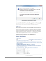
Uninstalling Total Access Statistics
Total Access Statistics supports the standard Windows installation protocol,
so uninstalling is similar to uninstalling other programs:
Start the Uninstall Process
From the Windows Start Menu, select Control Panel, then:
Windows Vista, Windows 7, and Windows 8

In the Programs section, select Uninstall a Program
Windows XP

Select Add/Remove Programs
Select Total Access Statistics for Removal
14  Chapter 2: Installation

Select Total Access Statistics from the list of installed programs

Click on Uninstall from the menu

The installation program loads. Choose Remove and follow the
prompts.
Total Access Statistics
After a few moments, the Total Access Statistics program files and its
registry entries are deleted.
Total Access Statistics Tables in Your Databases
Total Access Statistics also creates four tables in each database that you use
to generate Total Access Statistics scenarios. These tables contain
information about your analysis selections, and are not removed when you
uninstall the program. You may choose to delete them from your databases
manually, but you may want to keep them to preserve your scenarios if you
expect to use Total Access Statistics in the future. In general, these tables
are very small and do not interfere with your application.
If you do not need to keep your scenario settings, delete the four Total
Access Statistics tables that begin with “usysTStat” (usysTStatScenarios,
usysTStatOptions, usysTStatFields, and usysTStatParameters). These files
are hidden in your navigation pane. To see them, right click on the
Navigation Pane and select Navigation Options, and check the Show System
Objects option.
If you open Total Access Statistics but do not create scenarios, or if you
delete all scenarios before exiting Total Access Statistics, the hidden
scenario tables are automatically removed from your database when you
exit the program.
Total Access Statistics
Chapter 2: Installation  15
Chapter 3: Running Total Access Statistics
You can invoke Total Access Statistics interactively to design and run analysis scenarios, or
you can run the analysis programmatically from your VBA code. This chapter describes how
to start Total Access Statistics and run it interactively, the analysis types that are available,
and how to prepare your data to get the most out of Total Access Statistics.
Topics in this Chapter
 Important Concepts
 Starting Total Access Statistics
 Analysis Types
 Preparing Data
 Scenarios
 Calculation Accuracy
Total Access Statistics
Chapter 3: Running Total Access Statistics  17
Important Concepts
There are several important concepts you should be familiar with before
installing and using Total Access Statistics:

Total Access Statistics analyzes data in Access/Jet databases (MDB
and ACCDB files) and Access Data Projects (ADPs). The interactive
program is version specific and only runs with its version of Access,
but it runs on all database formats supported by that version.

Analysis is performed on the tables and queries in your database.
The tables may be Access tables or linked tables. The queries may
be select queries or crosstab queries. For ADPs, the data sources
may be tables, views, stored procedures, or user defined functions
that output data.

Results are stored in tables in your database. You can use these
tables like any other Access table (SQL Server tables in ADPs) and
add them to forms, reports, or other queries.

With the exception of analyses that you specify to place results in
your table, your data is never modified and temporary tables are
never created in your database. When it needs temporary tables,
Total Access Statistics creates them in its own temporary database.

Multiple fields and an unlimited number of records can be analyzed
at one time.

Groups of records can be analyzed separately. This is similar to
“Group By” in Access or SQL summary queries.

Records can be weighted by assigning a weighting field that
designates the number of times the record is counted.

Null values are automatically ignored. You can also specify specific
values or ranges of values to ignore.

Your analysis selections (scenarios) are automatically saved for
reuse. Only the settings are saved, not the data, so the latest data is
always used to recalculate the results when you run a scenario.

The scenario information is stored in four hidden system tables in
your database. The information remains with your database even if
you rename or move the database, re-install Total Access Statistics,
or upgrade to a new version.
18  Chapter 3: Running Total Access Statistics
Total Access Statistics
Tip: Using a Separate Database
Since Total Access Statistics creates output tables in the current database,
you may clutter your database with unnecessary tables. If you are
performing a lot of ad hoc analysis, consider creating a new database and
linking to your data tables. This keeps Total Access Statistics and its results
separate from your main database. If you are not familiar with using linked
tables, consult your Microsoft Access manual or help file.
If you plan to add Total Access Statistics features to your applications via
Visual Basic for Applications (VBA), you need to create your scenarios in
your application’s database (see page 155 for details).
Starting Total Access Statistics
Open the database with the data you want to analyze or a database that is
linked to the table(s). Make sure that you have the proper permissions to
the database — you must have rights to read and create tables.
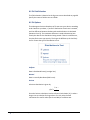
To begin, use the sample database (SAMPLE.MDB), located in the directory
where you installed Total Access Statistics. This database contains sample
tables and scenarios, and is a useful learning tool.
When you install Total Access Statistics, a link to the sample database is
created in your Windows Start menu:
All Programs, FMS, Total Access Statistics, Sample
Database
When you launch the sample database from this link, it always opens in
the correct version of Access, regardless of what Microsoft considers the
default for MDB files. This is accomplished using Total Access Startup
from FMS. Visit our website or contact us for more information.
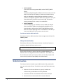
With the database open, launch Total Access Statistics from the Access
Database Tools, Add-ins ribbon:
Microsoft Access 2013 Add-ins Ribbon
Total Access Statistics
Chapter 3: Running Total Access Statistics  19
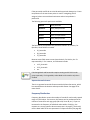
Microsoft Access 2007 and 2010 Add-ins Ribbon
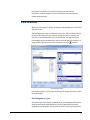
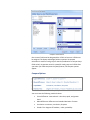
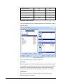
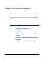
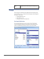
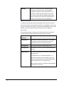
The initial screen of the Statistics Wizard appears:
Main Form
The main form of the Statistics Wizard controls the program. From here, you
can create, edit and run scenarios. The scenarios are organized by Analysis
Type:
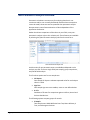
Analysis Type Tabs
When you click on the Analysis Type tabs, the corresponding page of
options and scenarios appears. Each of the analysis types has additional
types, which are displayed in the option group buttons on the left side of
the page. If you have existing scenarios, they appear in the list on the right.
When you click on a scenario to select it, the buttons below the list become
enabled to let you edit, copy, delete, get details, generate code, or run it.
See Chapter 4: Using the Statistics Wizard for details about the Statistics
Wizard.
20  Chapter 3: Running Total Access Statistics
Total Access Statistics
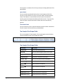
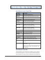
Analysis Types
All of Total Access Statistics’ features are organized in analysis type
categories. In general, every analysis shows the number of observations and
the number of missing (ignored) values. Details about each feature are
provided in future chapters, but a quick summary is provided below.
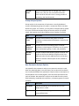
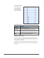
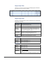
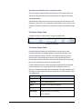
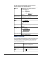
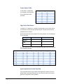
Parametric Analysis Options
Parametric analysis is performed on numeric fields that are assumed to be
continuous and normally distributed. Fields can be analyzed individually or
compared with each other.
Total Access Statistics
Type
Description
Describe
Analyze a numeric field: standard deviation, standard
error, variance, coefficient of variance, skewness,
kurtosis, geometric mean, harmonic mean, RMS, mode,
confidence intervals, t-Test vs. mean, percentiles, etc.
Frequency
For each field, analyze frequency distribution for each
interval (range of values): count, sum, percent of total,
cumulative count, percent, and sum.
Percentiles
Perform analysis similar to Describe, but place results in
records rather than fields (each percentile is a separate
record): Median, quartiles, quintiles, octiles, deciles, and
percentiles. Results can also be placed in a field in your
table with the percentile for each record.
Compare
Compare two fields: mean and standard deviation of
difference, correlation, covariance, R-square, paired tTest.
Matrix
Perform analysis similar to Compare, but rather than
comparing several fields to one, compare all fields to
each other creating a matrix.
Regression
Calculate simple, multiple, and polynomial regressions
with ANOVA and residual table. Estimated Y can be
placed in a field in your table.
Crosstab
Create cross-tabulation with row and column
summaries, and % of row, column, and total for each
cell. Chi-Square analysis is also available with expected
value and % of expected for each cell.
Chapter 3: Running Total Access Statistics  21
Running
Totals
Perform running totals such as average, sum, count,
median, min, max, etc. over a sorted list of records.
Totals can be for the entire list or a moving number of
records (e.g. the last 10 records)
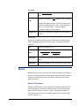
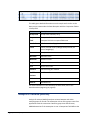
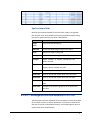
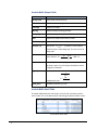
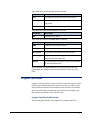
Group Analysis Options
Group analysis is the comparison of continuous, normally distributed
numeric data between groups of records. A comparison field in the table
defines the groups. For instance, you may want to compare data by gender
or by race. Unlike the Compare feature in Describe, which is for paired
values, these groups are usually of different sizes (number of records).
Type
Description
Two sample
t-Test
Compare means between two groups of records.
Calculations include pooled and separate t-values for the
two groups.
ANOVA
(analysis of
variance)
Compare the means of multiple groups of records.
Calculations include degrees of freedom, sum of squares
within and between groups, F-value, and probability.
Two way
ANOVA
Compare multiple fields between groups of records. The
results are the same as ANOVA, except that they have
additional values for each additional field. Use two way
ANOVA to measure relative impact of each variable on
the mean.
Non-Parametric Analysis Options
Less powerful than parametric analysis, non-parametric analysis is used
when the underlying data is not continuous, such as data that is ordinal or
not normally distributed. Non-parametric analysis makes no assumption on
the distribution of the underlying data, since the results are based on the
ranks of the data. Non-parametric analysis can be made for each numeric
field individually, compared with each other, or between groups of records
(samples).
Type
Description
Chi-Square
Evaluates distribution and expected value for each
unique value in a field.
Sign Test
Calculates a one sample sign test versus median, mean
or user defined value.
22  Chapter 3: Running Total Access Statistics
Total Access Statistics
K-S Fit
Performs Goodness of Fit tests to determine if a numeric
field fits a uniform, normal, or Poisson distribution.
2 Sample
Executes Wald-Wolfowitz Runs Test, Mann-Whitney U
Test, and Kolmogorov-Smirnov.
N Sample
Performs Kruskal-Wallis one way ANOVA.
Paired
Fields
Performs field comparisons: paired sign test, Wilcoxon
Signed Rank, Spearman’s Rho correlation.
N Fields
Calculates Friedman’s two way ANOVA.
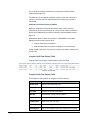
Record Analysis Options
Unlike other analysis types, Record Analysis features generate results that
manipulate your records directly. With options to update your existing
records or create new records similar to your data source, Record Analysis
helps you manage your data.
Type
Description
Random
Selects a random number or percentage of records from
your data.
Ranking
Assigns ranking values to your records and accounts for
ties.
Normalize
Normalizes an existing data source by creating a
separate record for each value in your specified fields.
Financial Analysis Options
Type
Description
Periodic
Cash Flows
Calculates the discounted values and rates of return for
cash flows with regular payment intervals.
Irregular
Cash Flows
Calculates the discounted values and rates of return for
cash flows with irregular, date specific, payments.
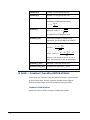
Preparing Data
To take full advantage of Total Access Statistics, it is best to follow these
guidelines:
Total Access Statistics

Use normalized data

Analyze one data source at a time
Chapter 3: Running Total Access Statistics  23
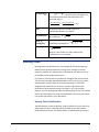
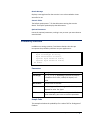
Using Normalized Data
Total Access Statistics uses the same principle as Microsoft Access queries,
which are optimized for normalized data. Rather than going into theoretical
discussions on data normalization, we present you with the basic idea. The
fundamental concept is to store your data in a format that supports using
summary queries, which allow Totals with Group By and Sum fields. Avoid
storing data across several fields (in spreadsheet format), since new
columns need to be added if new categories arise.
A normalized structure allows you to store data by adding records rather
than fields. In relational databases, records are free, but fields are
expensive.
Like Microsoft Access, Total Access Statistics does not perform “sums”
across fields, only within fields. If you need spreadsheet-type reports, use
the Total Access Statistics or Microsoft Access crosstab feature when
needed, but store your data in a normalized format.
Bad Non-Normalized “Spreadsheet” Data
Good Normalized Data
24  Chapter 3: Running Total Access Statistics
Total Access Statistics
Convert Data to Normalized Format
To manually convert data from a non-normalized format, you’ll need to
create a table with the proper structure, and use a series of APPEND queries
to fill the new table and delete records with blank values.
Fortunately, Total Access Statistics offers a Normalize feature under Record
Analysis that makes it easy to normalize your data. Learn more on page 127.
Analyze One Data Source at a Time
While you can analyze several tables during a Total Access Statistics session,
you can only analyze one table or query at a time.
In some cases, related data may exist in several tables. A select query
usually does the trick. For instance, if you have an Invoice and Customer
system and want to analyze invoices based on customer information (e.g.
sales by state), you need to combine the Invoice and Customer information
in a query prior to running Total Access Statistics (the Invoice record plus its
corresponding state or zip code).
In other situations, a query is unable to combine your data properly,
requiring you to create a new table, combine your data there, and analyze
that. For example, a separate table may exist for each year of sales. To
analyze this, create a table similar to the original tables with an additional
field designating the year, and fill it with your data.
If you want to analyze a subset of records, create a query with your criteria,
then use that as the data source for Total Access Statistics. If you perform
multiple analyses on the same data, you may find it more efficient to put
the query results in a table via a Make Table query, and have Total Access
Statistics analyze the resulting table.
Scenarios
Total Access Statistics saves each analysis as a scenario, which is saved in
four tables within the database where the analysis is run. A scenario stores
all information about the analysis, including the data source and fields to
analyze, the type of analysis to perform, any options within the analysis
type, the output table(s), and the description. A scenario does not store the
data that you analyze — the latest data is always used when you run a
scenario. Since results are not saved within your scenarios, you can easily
repeat an analysis on updated tables, modify your analysis, or share
analyses among users.
Total Access Statistics
Chapter 3: Running Total Access Statistics  25
Chapter 11: Advanced Topics provides more information about how
scenarios are saved. It also shows how to bypass the interactive Wizard
completely, and run your saved scenarios within your applications.
Calculation Accuracy
Total Access Statistics uses double precision (15 digits of accuracy) for all
calculations. Results are placed in Access tables, which show all decimal
places for each number. Probability values (0 to 100%) are presented as
decimal values between 0 and 1 (i.e. 48% is 0.48).
26  Chapter 3: Running Total Access Statistics
Total Access Statistics
Chapter 4: Using the Statistics Wizard
The Statistics Wizard guides you through the process of creating and running your scenarios.
No programming is required — just point and click to choose the table and fields to analyze
and the options to generate. This chapter provides details about using the Statistics Wizard
to create and run scenarios. Detailed information about each type of analysis is provided in
later chapters.
Topics in this Chapter
 Scenario Selection (Main Form)
 Creating a New Scenario
 Data Sources that Require Parameters
 Field Selections
 Ignoring Data
 Analysis Options
 Output Tables and Description
Total Access Statistics
Chapter 4: Using the Statistics Wizard  27
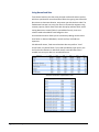
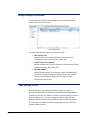
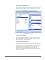
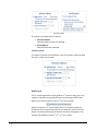
Scenario Selection (Main Form)
When you open Total Access Statistics from your Access Add-ins menu, the
Statistics Wizard Main Form appears:
Main Form
The analysis tabs across the top determine the list of scenarios displayed.
The analysis types are organized into Parametric, Group, Non-Parametric,
and Record options. When you select one of these tabs, the corresponding
sub-analysis types are displayed on the left side of the page. If you select
one of the subtypes (e.g., Describe, Frequency, Percentiles), only scenarios
of that particular type are shown. Select All to show all scenarios of the
selected analysis type.
The following buttons are available at the top of the Main Form:
Button Name
Description
New
Create a new scenario
Edit
Edit the currently highlighted scenario
Duplicate
Copy the current scenario
Delete
Delete the current scenario
Details
See detail information for the current scenario
Code
Generator
Generate code that you can paste into your module to
run a scenario programmatically. See Scenario Code
Generator on page 162 for details.
28  Chapter 4: Using the Statistics Wizard
Total Access Statistics
Run
Run the current scenario
Help
Display the help file
About
Display the About screen
Exit
Close the Total Access Statistics Wizard
Probability
Calculator
Show the Probability calculator for evaluating test
values (Z, Student’s t, Chi-Square, F). See Chapter 10:
Probability Calculator for more information
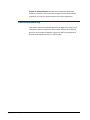
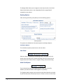
Creating a New Scenario
To create a new scenario, click the [New] button, and you will see the
following screen:
Select Analysis Type Form
Choose the type of scenario to create and press [Next] to go to the Select
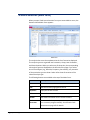
Source Object screen:
Select Data Source
Access Databases (MDBs and ACCDBs)
For Access Jet databases, you can select a table or query as your data
source. Tables can be tables in your database or linked tables from SQL
Server, dBase, Paradox, etc. Queries must be Select queries that return
records or Crosstab queries. For obvious reasons, action queries, which do
not return records, cannot be a data source.
Total Access Statistics
Chapter 4: Using the Statistics Wizard  29
Select Data Source for MDBs and ACCDBs
Select the table or query containing the data to analyze. The tabs across the
top allow you to select from a list of tables, queries, or both. Highlight the
data source you want and press [Next].
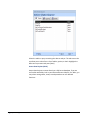
Access Data Projects (ADPs)
Access Data Projects connect directly to a SQL Server database. If you are
not familiar with ADPs, look in your Microsoft Access help file. For ADPs, you
may select among tables, views, stored procedures or user defined
functions:
30  Chapter 4: Using the Statistics Wizard
Total Access Statistics
Select Data Source for ADPs
Verifying Stored Procedures and User Defined Functions
If you choose a Stored Procedure or User Defined Function, a screen
appears to confirm you want to execute it. Stored Procedures and User
Defined Functions can do all sorts of things (like delete records) and not just
provide a set of records for analysis. You need to confirm the code behaves
as you expect and only returns records because Total Access Statistics may
need to execute it multiple times and it should not alter data:
Total Access Statistics
Chapter 4: Using the Statistics Wizard  31
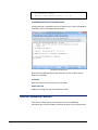
Review of Stored Procedure or User Defined Type Code
Confirm this is safe and valid before pressing [Next].
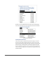
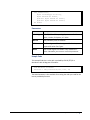
Data Sources that Require Parameters
If you select a query, stored procedure or user defined function that
requires parameters, a screen appears for you to enter the values:
Enter Parameter Values for Your Data Source
Each parameter is on a separate line with its data type. Enter your values in
the [Parameter Value] column.
For Access queries, you should explicitly define the parameters and their
data type under the Query, Parameters menu when the query is in design
mode. Otherwise, all your parameters will be treated as text strings.
For Boolean (Yes/No) fields, enter -1 for Yes (True) and zero for No (False).
32  Chapter 4: Using the Statistics Wizard
Total Access Statistics
Press [Next] to continue. If you edit an existing scenario that has
parameters, a button appears on the Field Selection form that lets you
change the parameters.
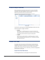
Field Selections
When you select [New] or [Edit], the Statistics Wizard takes you to the Field
Selection screen.
The Field Selection screen is divided into two parts. The left side allows you
to enter a description for this scenario, change the table to analyze, and
view the list of available fields in the selected table. The right side of the
form displays the fields selected for analysis and how they are assigned. To
assign a field, highlight it on the left, and press one of the
buttons.
Field Selection Form
Use the Sort options at the bottom of the form to change the order in which
the fields display.
Field Assignment Types
All analysis types have Group, Independent (X), and Weighting field options.
Analyses that require field comparisons (such as Regressions) have the
Dependent (Y) field option. The Comparison field is used for group analysis.
Total Access Statistics
Chapter 4: Using the Statistics Wizard  33
Crosstabs have a completely different set of options: Row Fields, Column
Field, Value Fields and Weighting Field. See page 71 for more information
on Crosstab options.
The right side of the form varies depending on the analysis type selected,
but there can be as many as five field types:
Group Fields
You can optionally select one or more Group fields to define unique sets of
records for analysis. This is similar to placing a “Group By” in the Totals
section of a query. With a Group By and Sum in a query, Access’s datasheet
(query output) includes a separate record for each unique Group By field’s
value. The same principle applies in Total Access Statistics. For every
combination of unique values in the group fields, a separate analysis (output
record) is generated. If no group fields are specified, every record in the
table is analyzed as one set.
Independent (X) Fields
X fields are the number fields (independent variables) to analyze. You must
select at least one X field.
Dependent (Y) Field
When you select an analysis type involving field comparisons, you must
assign a numeric value as the Y field. The Y field is the dependent variable
that each X field is compared against.
Weighting (W) Field
The Weighting field (variable) is an optional numeric field that allows you to
“Weight” each record. It is useful if your records contain summary
information. For instance, if each record is a country with [Population] and
[Average Age] fields, by assigning [Population] as the weight field and
[Average Age] as the X Field, you can calculate the statistics for all the
countries taking relative size into account. If the weight field is null or zero,
the record is ignored.
Comparison Field
Use a comparison field when performing group analysis and non-parametric
sample comparisons. The comparison field defines each sample set of
records (e.g. a Sex field with Male and Female values). This field is explained
in more detail in Chapter 6: Group Analysis on page 83.
34  Chapter 4: Using the Statistics Wizard
Total Access Statistics
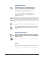
Selecting Fields for Analysis
Button to
assign a field
To assign a field to a particular type, highlight the field in the list,
and press the right arrow button in the box where you want to
assign the field. For instance, to assign the [State] field as a
Group field, click to highlight “State” in the Fields list, and then
click on the right arrow in the “Group Fields” box.
You can select multiple fields at once by selecting them with the
[Ctrl] button while you click, or a range of fields holding the
[Shift] button and clicking.
Double click on a field to automatically assign it. Numeric fields are
assigned to X Field, while other field types are assigned as Group fields.
Reordering Fields
For some fields such as Group and X fields, several fields may be assigned.
Move field up By default, the fields are processed in the order you select them, but you
can change this by using the up and down buttons. To move the selected
field, simply highlight the field you want to move and click on one of the
buttons.
Move field
down
Removing Fields from Analysis
To remove a selected field, highlight it and press the left arrow button, or
Un-assign one double click on it. You can select multiple fields at once by holding the [Ctrl]
button while you click.
field
Un-assign all
fields
You can remove all the fields of a particular type by pressing the large left
arrow.
Finishing
After selecting the fields, press [Next] to display the analysis type options.
If you decide not to proceed, press [Back] to cancel changes and return to
the main form.
Total Access Statistics
Chapter 4: Using the Statistics Wizard  35
Ignoring Data
Total Access Statistics automatically ignores null values during analysis. By
default, all non-null values are used in the calculations, but there may be
times when you want to ignore a specific value or range of values. Total
Access Statistics includes a powerful feature that allows you to do this.
Press the [Ignore] button on the field selection form:
Ignore Values Form
Ignoring a Specific Value
In some situations, you may use a dummy value rather than or in addition to
nulls (for instance 999). This is useful when you want to designate a value is
unknown rather than not filled. In this instance, you want to keep the
dummy value out of your calculations and treat it as a missing value. To
specify a value to ignore, choose the option to “Ignore a Specific Value” and
enter the value to ignore.
Ignoring a Range of Values
Alternatively, you may want to limit your analysis to a range of values. You
can choose to ignore all values above a certain value, below a value, or
both. Select the “Ignore a Range of Values” option and enter the values in
the two fields. Values equal to the number you enter are not ignored, so if
you want to ignore values greater than and equal to a value (e.g. 100), enter
a value slightly smaller (99.999999).
36  Chapter 4: Using the Statistics Wizard
Total Access Statistics
What Values are Ignored
When Ignore options are set, they are applied to the Independent (X) and
Dependent (Y) fields. If a Comparison field is numeric it also respects the
ignore options. The Weighting (W) field is affected if a Specific value is
ignored, but ignoring a range of values does not affect weightings.
Values in Group fields are not affected. Group fields can be any field type
and create separate records for each group in the output table. Calculations
of each group are entirely separate, so there is no problem with Groups of
invalid values. You can easily ignore the records you do not want in the
output table.
Impact on Analysis with Updated Records
There are a few calculations with the option of updating a field in your data
source:

Percentiles
The percentile value of the record

Regressions
The estimated Y value of the record

Running Totals
The running total of the record

Random
Whether the record is selected

Ranking
The rank value of the record
When you ignore a specific value or a range of values, the skipped records
are not updated. Therefore, the data that existed in the update field for
those records is unchanged.
This may cause confusion, so to avoid mixing the new information with
existing information in the ignored records, you should clear the field for all
your records before running the scenario.
There are situations when you may not want to clear the data. For
instance, you may be combining data from multiple ranges of ignored
(non-overlapping) values in that field.
Analysis Options
After you assign the fields to analyze, press the [Next] button to display
other analysis options.
Total Access Statistics
Chapter 4: Using the Statistics Wizard  37
The options available vary depending on the analysis type selected. Options
for each type of analysis are discussed in future chapters.
Options Form
After choosing the options desired, press [Next] to continue.
Check Boxes
Click on a check box to select the option, and click on it again to unselect it.
Each check box is independent of other options.
Option Group Buttons
Options group buttons are linked to each other, and you can only select one
option in the group.
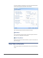
Output Tables and Description
When you press [Next] on the analysis option screen, you see the following
screen:
38  Chapter 4: Using the Statistics Wizard
Total Access Statistics
Output Table Form
Enter a name for the output table(s) to be generated. By default, each
analysis type’s output table has a unique name. The table is created in your
current database. You can change the name to any valid Microsoft Access
table name.
You can optionally add a scenario description to help you remember details
about the analysis. This description is saved with the scenario and can be
viewed from the main screen of the Wizard.
When you finish, press [Save] to save the scenario and return to the main
screen of the Wizard, or press [Save and Run] to save and run the scenario.
If the output table already exists, a message appears asking for permission
to overwrite it.
If the scenario is successful, the output tables are created and displayed.
Use these tables like any other Microsoft Access table: search, reformat
fields, export, etc. You can also use the Access AutoReport feature to create
a report. When you are finished examining the output, close the tables and
return to the Statistics Wizard for additional analysis.
Total Access Statistics
Chapter 4: Using the Statistics Wizard  39
Chapter 5: Parametric Analysis
This chapter describes Total Access Statistics’ parametric analysis options. Parametric
analysis should be performed on continuous numeric fields where data is assumed to be
reasonably normally distributed. Numeric data that does not satisfy these conditions should
be analyzed with non-parametric tests.
Topics in this Chapter
 Parametric Analysis Overview
 Describe (Field Descriptives)
 Frequency Distribution
 Percentiles
 Compare (Field Comparisons)
 Matrix
 Regression
 Crosstab and Chi-Square
 Running Totals
Total Access Statistics
Chapter 5: Parametric Analysis  41
Parametric Analysis Overview
The Parametric Analysis features are available when you select the
[Parametric Analysis] tab from the main form:
Parametric Analysis Tab
The types of parametric analysis are listed on the left:
42  Chapter 5: Parametric Analysis

Describe (Field Descriptives)
Analyze all X fields you specify, customizing the statistical values
that are calculated.

Frequency Distribution
Determine the number of occurrences within each range of numeric
values.

Percentiles
Determine the percentiles for each Group and X field you select.

Compare (Field Comparisons)
Perform a record-by-record comparison between each X field and
the specified Y field.

Matrix
Perform calculations similar to Compare, but with a quick way to
look for correlations and other relationships between many fields.

Regression
Calculate the least squares (best fit) curve to determine an equation
that relates the Y (dependent) variable to the X (independent)
variable(s).

Crosstab and Chi-Square
Create matrices showing summaries of one field across two fields,
and optionally measure the independence of the two variables.
Total Access Statistics

Running Totals
Perform running totals such as average, sum, count, median, min,
max, etc. over a sorted list of records. Totals can be for the entire
list or a moving number of records (e.g. the last 10 records)
Describe (Field Descriptives)
Describe allows you to analyze all X fields you specify, creating the following
statistical values:

Count, Missing, Mean

Minimum, Maximum, Range

Variance, Coefficient of Variance, Standard Deviation, Standard
Error

Sum, Sum Squared

Geometric Mean, Harmonic Mean, Root Mean Square

Skewness, Kurtosis

Mode, Mode Count

Confidence Intervals using t or Normal distribution

t-Test versus Mean

Percentiles (Median, Quartiles, Deciles)

Frequency distribution
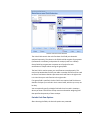
Field Selection
On the Field Selection form, you can select multiple Group and Weight fields
in addition to choosing X fields. Separate calculations are made for each
group (combination of unique Group fields values), and a separate record is
created for each group and X field.
Total Access Statistics
Chapter 5: Parametric Analysis  43
Describe Field Selection Form
See page 33 for details about the Field Selection form. After selecting fields,
press [Next], to display the Describe options.
Describe Options
Describe Options
When you select a check box, the corresponding fields are generated. See
page 37 for details about the Options form.
44  Chapter 5: Parametric Analysis
Total Access Statistics
When you finished, press [Next] to specify the output table and description
(described on page 38).
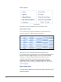
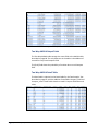
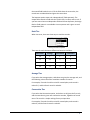
Describe Output Table
Following is an example of an analysis of three X fields (Age, Weight,
Cholesterol) grouped by State (not all fields are shown):
Describe Output Table
Describe Output Fields
The following fields are always created for the Describe analysis:
Field Name
Description
Group Fields
Group fields selected (if any)
DataField
X field name identifying the data in the record
Count (N)
Number of non-Null X field records (or if Weight field
specified, the sum of weightings)
Observations
Number of X field records (different from N).
This field is only created if Weight field specified.
Missing
Number of blank X field records
Mean (x )
x  x N
Sample mean and an estimate of the population mean
(µ)
The following sections list the fields that are created if its checkbox is
selected:
Minimum, Maximum, Range
Total Access Statistics
Minimum
Smallest value in X field
Maximum
Largest value in X field
Range
Range of values in the field = Maximum - Minimum
Chapter 5: Parametric Analysis  45
Variance Fields
There is an option for calculating these values using an N-1 or N method.
The variance divisor depends on the method selected. The N-1 method
creates an “adjusted” (unbiased) sample variance as corresponds to the
Access VAR( ) function. The N method is for a population variance and is
equivalent to the VARP( ) function. The N-1 Method is preferred when the
data represents a portion (sample) of the entire population. For large N (N >
30), both definitions result in similar numbers.
Variance (s2)
 x
i
 x 2
N 1
 x
or
i
 x 2
N
Variance is a measure of the distribution of the data
from its mean. It is a data point’s average squared
difference from the sample mean. The formula depends
on the method selected.
CoeffOf
Variance
Coefficient of Variance  s
StdDeviation
(s)
Standard Deviation is the square root of variance
StdError (SE)
Standard Error of the Mean = s
x
This removes the effect of a larger variance due to larger
means.
N
Regardless of whether the population is normally
distributed, the sample means ( x ) should be normally
distributed. Standard error measures the standard
deviation of x to the population mean. As sample size
increases, x approaches population mean and standard
error decreases.
Sum, Sum Squared
Sum
46  Chapter 5: Parametric Analysis
Sum of X values
x
x
SumSquared
Sum of squared values 
AdjSum
Squared
Adjusted sum squared   x 2 N
2
The mean squared value.
Total Access Statistics
Means: Geometric, Harmonic, RMS
Geometric
Mean
N
 log(x) 

X 1  X 2  X 3  ...  X N  exp


N


Geometric Mean is used for a variable that has a constant
rate of change; that is, as the mean increases, so does its
variance. A logarithmic transformation eliminates this
effect. The geometric mean is undefined if any X value is
zero or negative.
Harmonic
Mean

N
 1 x 
Harmonic Mean
The Harmonic Mean is the mean of a reciprocal
transformation, and is often used to analyze ratios. It is
undefined if any X value is zero or negative.
x
RMS
2
N
Root Mean Square =
Root Mean Square, or quadratic mean, is often used in
physical systems. It is the mean of the square
transformation.
For positive values of X, H.M.  G.M.  x  RMS
Skewness, Kurtosis
Skewness

N
 xi  x 



(N  1)(N  2)  s 
3
Skewness measures the symmetry of the data. A normal
distribution (bell curve) has zero skewness. If it has a
longer tail to the right of the mean, it is skewed to the
right and has positive skewness. Negative skewness
indicates skew to the left.
SE_Skewness
Total Access Statistics
Standard Error of Skewness depends on sample size, not
data values.
Chapter 5: Parametric Analysis  47
Kurtosis
4


N
(
N

1
)
x

x
3N  12


i





 (N  1)(N  2)(N  3)   s   N  2N  3


Kurtosis measures the peakedness of the data. A
normally distributed sample has a Kurtosis equal to zero.
A highly peaked distribution is called leptokurtic and has
positive kurtosis. A relatively flat (thick tailed)
distribution is called platykurtic and has negative
kurtosis. A moderately peaked distribution is called
mesokurtic.
SE_Kurtosis
Standard Error of Kurtosis depends on sample size, not
data values.
Mode, Mode Count
Mode
Mode is the most common value. If a tie exists for
multiple values, there is no mode.
Mode Count
Mode Count is the occurrences of the Mode. If there is
a tie, this value is shown, but Mode is blank.
Confidence Intervals
Confidence Intervals Options
Confidence intervals are used to estimate the population mean from sample
data. The sample is assumed to contain sampling variability, so its mean is
not necessarily the population mean. Confidence intervals estimate the
value of the population mean with an expected degree of accuracy. For
instance, one may describe the mean as having a 95% chance of being 52 ±
5, where 95% is the confidence interval, 52 is the sample mean, and 5 is the
confidence interval band width. As the sample size increases, this band
becomes smaller. Similarly, the band increases as the confidence interval
(%) increases.
Intervals
There are two possible confidence intervals to select. You can either select
the check box for the 95% interval or type in your own interval (between 1
and 99.999%). Type in whole numbers (e.g. type 50 for 50% not 0.5).
48  Chapter 5: Parametric Analysis
Total Access Statistics
Two techniques may be used:
t-Test
The t-Test (sometimes called the Student’s t) is a distribution that changes
with sample size. For small samples (N < 30), t-Tests are considered the
most robust test. For large samples (N > 30), t-Test yields results similar to
the normal distribution test. The t-Test uses the sample standard deviation
to determine the confidence interval. This always results in a wider interval
than that of the Normal distribution option.
Normal
The Normal distribution test provides a more accurate result, but requires
knowledge of the standard deviation of the population. Enter this value in
the Std. Dev. field. If you selected more than one X field, and each X field
has different standard deviations, you need to run a separate scenario for
each X field.
These are the confidence interval fields created:
Field Name
Description
n% T Band
Band width for t-Test, where n is the confidence
interval. For Normal distribution the field is n% N Band.
n% Upper
Upper limit = (mean + band)
n% Lower
Lower limit= (mean - band)
t-Test vs. Mean
t-Test vs. Mean Options
This feature is sometimes called a one-group or one-variable t-Test and is
used to compare each X field to a hypothetical mean. The result indicates
the probability that the sample has the hypothetical mean. Enter the mean
to test in the field.
Both 1-tailed and 2-tailed probabilities are calculated. A 2-tailed test is used
to determine if the sample mean is significantly different from the
hypothetical mean (greater than OR less than). A 1-tailed test is only
concerned with the difference on one side (e.g. Is the sample mean
significantly greater than zero?).
Total Access Statistics
Chapter 5: Parametric Analysis  49
Field Name
Description
Population
Mean
Population mean being tested (your input value)
t-Value
 N
x  Population Mean 
s
where N is the count of the group and s is the sample’s
standard deviation calculated by the N-1 method
Prob (1-tail)
Statistical probability (0-1) that the sample mean is the
same as the [Population Mean]. If the probability is too
small (e.g. less than 1% or 5%), the hypothesis is
rejected. Probability is calculated from the t-Value and
degrees of freedom (N - 1).
Prob (2-tail)
2-tailed probability that the sample mean is the same as
the [Population Mean]. This probability is used when
there is no a priori reason to assume the sample mean
will be greater than or less than the population mean.
Percentiles
Percentile Options
To create Percentile calculations, select the percentiles check box, and
choose the type of Percentiles to calculate.
Percentiles are calculated by sorting the data from smallest to largest. The
middle value is the median (50th percentile). Dividing into 4 groups gives
quartiles (25th, 50th, and 75th percentiles), and 10 groups give deciles. This
is the formula used to determine which record is selected:
 Percentile
N  1  1
 100

Where N is the number of items, and Percentile a number between 0 and
100. For instance, for a sample size of 13, the quartile records for the 25th,
50th, and 75th percentiles are 4, 7, 11. By definition, the 0th and 100th
percentiles are the lowest and highest values.
50  Chapter 5: Parametric Analysis
Total Access Statistics
If the percentile cutoffs do not coincide with a particular data point, a linear
interpolation of the two closest points is used. If a weighting field is
assigned, values are considered continuous and no interpolation is
performed.
The following percentile options are available:
Median
50th percentile
Quartiles
Every 25th percentile
Quintiles
Every 20th percentile
Octiles
Every 12.5 percentiles
Deciles
Every 10th percentile
5th Percentiles
Every 5th Percentile
The field names correspond to the percentile number. For instance, for
Quartiles, these fields are created:

25_Percentile

50_Percentile

75_Percentile
Because Access field names cannot have decimals, for Octiles, the .5 is
represented by -5. For instance, its field names include:

12-5_Percentile

37-5_Percentile

etc.
Calculating Mode and Percentiles requires sorting each X Field in each
group separately. For large tables, select Mode or Percentiles only when
needed.
Separate Percentile Feature
There is a separate Percentiles feature outside this Describe section, which
has some different calculations and output table format. See page 55 for
more details.
Frequency Distribution
Frequency distribution counts the number of records for each evenly spaced
range of X field values. For instance, this feature can let you determine the
number of records for each age group (20 to 30, 30 to 40, etc.). If you are
interested in the frequency of individual values within a field (e.g. the
response to a survey question where answers are 1 through 5), you should
use the detail table of the non-parametric Chi-Square feature (see page 95).
Total Access Statistics
Chapter 5: Parametric Analysis  51
Frequency Distribution Options
Frequency Distribution creates a field for each data interval, and counts the
number of occurrences in each. You can select two types of output: Count
and Percent. Count is the number of occurrences, and Percent is the Count
as a percentage of total occurrences in the group. These are the options:
Number of Intervals
Determines the number of frequency intervals (fields) to create.
Include in Each Interval
Determines to which group an interval “boundary” value belongs. Lower
places the value in the lower limit of the interval (x <= N < z), while Upper
makes the intervals x < N <= z. For example, with Lower, 20 is placed in the
interval 20-30. Upper places the value in the interval 10-20.
Display Type
Count displays the number of occurrences in each interval. Cumulative
displays the number of occurrences in each interval plus all the previous
intervals. The Percent fields also reflect the choice selected.
Groupings
Specify the grouping intervals for calculating frequency. Default calculates
an initial value and width interval to accommodate all the data points for
the number of intervals specified. However, the intervals may not be the
most desirable groupings since the interval width would rarely be a nice
round number. If you select Specified, two fields appear, [Initial Value] and
[Width], to let you specify the exact initial value (start of the first interval)
and the interval width. By default, Total Access Statistics creates two
additional intervals for the count of items so that no records are skipped:
less than the initial value and greater than the maximum interval.
The following frequency fields are created:
52  Chapter 5: Parametric Analysis
Total Access Statistics
Field Name
Description
N <= x
The count of records (or weightings) with values less
than or equal to x (first interval value). This field is
created if Groupings = Specified.
y <= N < y + w
The count of records (or weightings) with values
between y and y + w (width). There is one of these
fields for each of the intervals.
z <= N
The count of records (or weightings) with values
greater than z (last interval value). This field is created
if Groupings = Specified.
For percentages, the field names use “%” rather than “N”.
Frequency Analysis Type
From the main Statistics Wizard screen, there is a Frequency analysis type
that is separate from Describe. That frequency feature has additional
options and presents the results differently. Read the next section for more
information.
Frequency Distribution
Frequency analysis determines the number of occurrences within each
range of numeric values. If you want to determine the count of specific
values rather than ranges, use the non-parametric analysis Chi-Square (see
page 95). The detail table of Chi-Square gives a result similar to the
Frequency table.
Difference from Describe
The Frequency feature here differs from the frequency calculation in
Describe (described on page 51) in these ways:
Total Access Statistics

The Frequency feature always calculates count, cumulative and
percent of total and cumulative values. Describe requires you to
choose count or cumulative.

Results are shown with each interval as a separate record with
information for each interval shown in one record side-by-side.
With Describe, results are in one record with each interval as a
separate field, so examining an interval’s count and percent of total
is more difficult.

The Frequency feature provides the option to calculate the sum and
percent of sum.
Chapter 5: Parametric Analysis  53
Frequency Field Selection
The Frequency field selection is identical to Describe field selection. Choose
as many X fields as you want. Group and Weight fields are optional. Since
the frequency intervals are identical for all the X fields, choose fields with
similar values. For instance, using the same intervals for Age and Annual
Income would be meaningless since the values are so different.
Frequency Options
Frequency Options
Refer to page 51 for details on Number of Intervals, Include in Each Interval,
and Groupings. In addition to these features, you can optionally choose to
calculate Sum of Values.
Frequency Output Table
This example is an analysis of the Age field, grouped by State, with 5
intervals, lower option, specified initial value of 25, and interval width of 10.
Since specified values were provided, two extra intervals before and after
the range are added for a total of 7 intervals:
Frequency Output Table
Frequency Output Fields
These fields are always created:
54  Chapter 5: Parametric Analysis
Total Access Statistics
Field Name
Description
Group Fields
Group fields selected (if any)
DataField
Field name identifying the data in the record
Interval
Interval number (1 to number of intervals)
Low<Range
Interval range’s low value. If Lower option is
selected, the field is [Low<=Range]
Range<High
Interval range’s high value. If Upper option is
selected, the field is [Range<=High]
Count
Number of records (or weightings) in interval
Count%
Percent of interval’s count to total count of group
Cumulative
Sum of count for this and all previous intervals in
group
Cumulative%
Cumulative sum of percentages
Sum of Values
This option creates these additional fields:
Sum
Sum of X field values in each interval (adjusted for
weightings if specified)
Sum%
Percent of interval’s sum to total sum for group
CumulativeSum
Sum for this and all previous intervals in group
CumulativeSum%
Cumulative percentage of cumulative sum
Percentiles
Percentile analysis determines the percentiles for each Group and X field
you select. It uses the same formula as the Percentile calculation in the
Describe section (explained on page 50).
Difference from Describe
The Percentile analysis type differs from the percentile calculation under
Describe in these ways:

Total Access Statistics
Results are shown with each percentile as a separate record. In
Describe, results are in one record with each percentile as a
separate field.
Chapter 5: Parametric Analysis  55

The minimum and maximum values are displayed (0th and 100th
percentiles).

There are options to calculate every percentile (0 through 100) and
every 0.5th percentile.

Percentiles can be assigned to individual records to a field in your
data source.
Percentile Field Selection
The Percentile field selection is virtually identical to the field selection of
Describe and Frequency. Choose as many X fields as you like. Group and
Weight fields are optional. Unlike frequency intervals, however, percentiles
are unique to each field, so it does not matter if the X fields are of similar
values or not.
Percentile Options
Percentile Options
The percentile options are divided into two sections depending on where
you want the results. If you want the results in an output table, check the
Create Output Table option. If you want to assign the percentile value to a
field in your data source, check the Assign Percentile to Field option and
specify the field name where the results should be placed. You may select
one or both options.
56  Chapter 5: Parametric Analysis
Total Access Statistics
Create Output Table
Percentile Calculation Options
Every percentile type generates the 0 and 100th percentiles (lowest and
highest values). Based on your selection, these percentiles are also
calculated:
Total Access Statistics

Median for the middle value (50)

Quartiles for 4 groups (25, 50, 75)

Quintiles for 5 groups (20, 40, 60, and 80)

Octiles for 8 groups (12.5, 25, 37.5, 50, 67.5, 75, and 87.5)

Deciles for 10 groups (10, 20, 30, through 90)

Percentiles for 100 groups (1, 2, through 99)

X.5 Percentiles for 200 groups (0.5, 1, 1.5, through 99.5)
Chapter 5: Parametric Analysis  57
Percentile Output Table
This example shows
octile calculations for
the Age and Weight
fields, grouped by State:
Percentile Output Fields
Field Name
Description
Group Fields
Group fields selected (if any)
DataField
Field name identifying the data in the record
Percentile
Percentile number: a value between 0 and 100
depending on which percentile type was selected
Value
Value corresponding to the percentile
Assign Percentile to Field
Percentiles can also be assigned to the individual records of your data
source. This option is only available if you selected one field to analyze and
your data source is updatable.
Your data source also needs a field where the percentile value is placed.
This must be a numeric field and may be an integer or double. Specify the
field name:
58  Chapter 5: Parametric Analysis
Total Access Statistics
Select an Existing Field in the Data Source to Update
By default, the field is updated with the Percentile value corresponding to
each record’s data value. You can also specify other Percentile calculations:
Fill with Percentile Type Option
Handling Tied Percentile Values
There is also an option to specify which percentile to assign to a record if
the record’s value equals multiple percentiles. For instance, there may be
several records tied for the highest value (100th percentile). That value could
represent the 96th to 100th percentile. By choosing to assign the low value,
the record would be assigned 96 (no other records would be assigned 97 to
100). By choosing the High option, they would all be assigned 100, and there
would be no 96-99.
Total Access Statistics
Chapter 5: Parametric Analysis  59
Percentile Field Assignment
This example shows the percentile value of
each Age in the AgePercentile field.
The percentile field is only updated for the
records analyzed. If the data field has null
values, you specified records to ignore, or used
a query that filtered records, be sure to clear
the percentiles field to avoid mixing old data
with the new data.
Compare (Field Comparisons)
Compare performs a record-by-record comparison between each X field and
the specified Y field. If the Y field is blank, the record is skipped. If the Y field
exists and the X field is blank, the record is skipped for that X field
calculation, but not for other X fields that exist. The output table contains a
record for each combination of check fields and X field.
Compare Field Selection
The Compare field selection screen differs from the previous screens with
the addition of a Y field option:
60  Chapter 5: Parametric Analysis
Total Access Statistics
Compare Field Selection
One numeric field must be designated the Y field. At least one X field must
be assigned. The Group and Weight fields are optional. A separate
calculation is made for each group of records (combination of unique Group
fields values). A separate record is created for each group and X field. After
you select your fields and press the [Next] button, the Compare options
appear.
Compare Options
Compare Options
You can create the following statistical values:
Total Access Statistics

Count Difference: cases where X is less than, equal, and greater
than Y

Mean Difference: difference and standard deviation of means

Correlation: covariance, correlation, R-square

Paired t-Test: degrees of freedom, t-value, probability
Chapter 5: Parametric Analysis  61
Compare Output Table
Following is an example of comparing Age and Weight against Cholesterol
grouped by State (not all fields are shown):
Compare Output Table
Compare Output Fields
By default, the following fields are always created (formulas are adjusted for
Weight field if specified):
Field Name
Description
Group Fields
Group fields selected (if any)
DataField
Field name identifying the data in the record
Count of
Y Field (N)
Count of X field values (if Weight field specified, the
sum of weightings) where X and Y are not blank. The Y
field name is included for reference.
Observations
Number of X field records (different from N).
Only created if Weight field specified.
Missing
Number of records with blank X or Y fields
Count Difference
Count < Y
Count of cases where X < Y
Count = Y
Count of cases where X = Y
Count > Y
Count of cases where X > Y
Mean Difference
MeanX
Mean of the X field
MeanY
Mean of the Y field
MeanDiff
Mean difference between X and Y
StdDevDiff
=
sx2  sy2  2  COV
Standard deviation of the difference between X and Y
62  Chapter 5: Parametric Analysis
Total Access Statistics
Correlation
Covariance

N  (xy )   x  y
N(N  1)
COV
Correlation
(R)
Pearson’s Correlation 
COV
, where s x and s y are the
s x sy
standard deviation of X and Y. Correlation measures the
relationship between X and Y, and is a value between -1
and 1. 1 is an exact match, -1 a perfect negative
correlation, and zero is no correlation.
R-Square (R2)
Square of the correlation. R-Square is a value between
0 and 1.
Paired t-Test
The Paired t-Test determines if the X and Y fields have statistically similar
means. Probabilities greater than 5% are usually accepted as statistically
significant.
t-DF
Degrees of freedom = (N - 1)
Paired tValue
t
MeanX - MeanY
s  s 2
2
x
2
y
N

MeanX - MeanY
StdDevX - Y
N
Prob (1-tail)
One-tailed probability (0-1) that X and Y have the same
mean
Prob (2-tail)
Two-tailed probability that X and Y have the same mean
Matrix
Matrix performs the same calculation as Compare but offers a quick way to
look for correlations and other relationships between many fields. Compare
compares several X fields to one Y field. Matrix compares all the X fields
against each other.
Matrix Field Selection
The Matrix field selection screen is identical to the Describe field selection
screen (see page 43). Choose the X fields to analyze. The matrix becomes
larger as more X fields are selected — keep in mind that the number of
calculations and amount of time needed increases with the square of the
number of X fields ( N 2 ) .
Total Access Statistics
Chapter 5: Parametric Analysis  63
Matrix Options
Matrix Options
Each selection creates a separate matrix comparing the fields.
Matrix Output Table
This is a matrix of Age, Weight and Cholesterol grouped by State with
Correlation, R-Square, t-Value and Prob (2-tail) options:
Matrix Output Table
Each matrix is a set of records identified by the [CalcType] field.
The correlation matrix is symmetrical (i.e. the correlation between Age and
Weight is the same as Weight and Age). This is true for Count, Missing,
Covariance, Correlation, R-Square, Std. Deviation Difference, and
Probability. Mean Difference and Paired t-Value produce negatively
symmetrical matrices (i.e. Mean X-Y of Age to Weight is the negative of
Weight to Age). Definitions of these calculations are given in the Compare
section on page 60.
Matrix Output Fields
The output table for Matrix always includes these fields, regardless of which
options are selected:
64  Chapter 5: Parametric Analysis
Total Access Statistics
Field Name
Description
Group Fields
Group fields selected (if any)
DataField
Field name identifying the data in the record
CalcType
Type of calculation:
X Field Names
 Count
 Correlation
 Missing
 R-Square
 MeanDiff
 t-Value
 StdDevDiff
 Prob (1-tail)
 Covariance
 Prob (2-tail)
Name of the X Field. The value in this field is the
CalcType comparison with the field in DataField
Regression
Regression calculates the least squares (best fit) curve to determine an
equation which relates the Y (dependent) variable to the X (independent)
variable(s). The field selection screen is identical to that for Compare on
page 60.
Choose among three regression types and two calculation options:
Regression Types
Regression Type and Calculation Options
Simple y  Ax  C
where A and C are the constants that are solved. “A” is the slope of the line,
“C” is the y-intercept. A linear (simple) regression is calculated between the
Total Access Statistics
Chapter 5: Parametric Analysis  65
Y field and each X field. Any record with a blank X or Y field is ignored. One
equation (record) is created for each set of group fields and X field.
Multiple
y   A n xn  C = A1 x1 + A2 x2 + C
where xi is the ith X field, and Ai and C are constants. A multiple regression of
the linear combination of X fields to the Y field is calculated. All X fields are
assumed to be independent variables. At least two X fields must be
assigned; otherwise you should use simple regression. Any record with a
blank X field or Y field is ignored. One equation (record) is created for each
set of group fields.
Polynomial
y   A n x n  C = A1 x + A 2 x 2 + ... + AN x N + C
where N is the polynomial order, and Ai and C are constants. A polynomial
regression between each X field and Y field is calculated. The polynomial
order (up to 9) determines the maximum power (exponent) of X in the
equation. Any record with a blank X or Y field is ignored. One equation
(record) is created for each set of group fields and X field.
Calculate Y-Intercept
This option controls whether the y-intercept (C constant) is calculated or set
to zero (through the origin). If this option is checked, the y-intercept is
calculated.
Calculate Regression ANOVA
If this option is selected, each regression’s ANOVA values are calculated.
The field names are described later.
Result Options
Regression Result Options
Create Residual Table
If this option is selected, a separate Residual table is created. The residual
table contains one record for each data point used in the regression
66  Chapter 5: Parametric Analysis
Total Access Statistics
calculation along with residual information. The Residual is the difference
between the actual Y and the regression’s estimated Y value.
Assign Estimated Y to Field
The value of Y based on the regression equation can be inserted directly
into a field on each record. This feature is available when only one
regression equation is being created for each record. This is always the case
for a multiple regression. For simple and polynomial regressions, this exists
if only one Independent (X) field is selected.
Simply specify the field where you’d like the result to be placed. The field
should be a double and the data source must of course be updateable.
Regression Output Tables
The following examples are different types of regressions for comparing X
fields [Age] and [Weight] against Y Field [Cholesterol], grouped by [State]
(not all fields shown).
Simple Regression Output Table
Multiple Regression Output Table
Polynomial Regression (Order 3) Output Table
Regression Output Fields
Regardless of which options are selected, the output table for Regression
always includes these fields:
Total Access Statistics
Field Name
Description
Group Fields
Group fields selected (if any)
DataField
Field name identifying the data in the record
Chapter 5: Parametric Analysis  67
Count of Y Field
Number of data points in group, where Y Field is the
name of the Y field
Missing
Missing number of records
Multiple R (R)
Square root of R-Square
R-Square (R2)
1
ResidualSumof Squares
TotalSumof Squares
RegressionSumof Squares
TotalSumof Squares
R-Square measures the proportion of variation in Y
that is explained by the regression. R-Square is
between 0 and 1 (1 is a perfect fit).

Adj_R-Square
 R2 
Adjusted R-Square
1  R 
2
N  2
StdError_of_
Estimate
Standard error of the Y estimate (regression) is the
standard deviation of the residuals.
Y-Intercept
Y-Intercept value, if this option is selected
Coef_of_X
Coefficient(s) of regression equation
The regression coefficient fields vary depending on the type of regression
selected:

Simple Regressions: one field for the X coefficient.

Multiple Regression: one field for each X field:
Coef_of_X1, Coef_of_X2, Coef_of_X3, etc.

Polynomial Regressions: one field for each polynomial order:
Coef_of_X^1, Coef_of_X^2, Coef_of_X^3, etc.
Coefficient Analysis
In addition to the Y-Intercept and equation coefficients, four other fields are
calculated for each coefficient to determine the accuracy and relative
importance of each coefficient. The four fields are explained below with the
field names in brackets:
Standard Error of Coefficients [SE_of_X]
Standard Error of Coefficients is a measure of each coefficient’s variability.
Although the coefficient is calculated, the sample data is assumed to
contain variability. The population coefficient is the sample coefficient plus
or minus the standard error.
68  Chapter 5: Parametric Analysis
Total Access Statistics
Beta Value of Coefficients [Beta_of_X]
Beta Value of Coefficients (also known as standardized regression
coefficients) shows the relative importance of each coefficient in the
regression equation. For multiple and polynomial regressions, it can be
misleading to examine only the unstandardized coefficients for importance.
A large coefficient may have little impact if its variable does not vary much.
The Beta removes this effect. Beta is not calculated for the Y-Intercept.
Betai  Ai si sy 
where Ai is the coefficient of variable i
si is its standard deviation, and
sy is the standard deviation of Y
t-Value of Coefficients [t-Value_of_X]
The t-Value of the coefficient is used to determine (via t-Test) the
probability that the coefficient value is significantly different from zero. tValue is the ratio of the Coefficient to its Standard Error.
Probability of Coefficients [Prob_of_X]
Probability of coefficients determines the probability that the coefficient is
zero based on its t-Value.
Regression ANOVA
The regression ANOVA indicates how much of the data variance is due to
the regression, and how much is not (residual). If the regression has a poor
“fit” (large residual), the F-Value is small and the probability that all
regression coefficients are zero (the null hypothesis) approaches 1. These
are the ANOVA fields:
Field Name
Description
Regression_DF (DF1)
Regression degrees of freedom. Number of
independent variables.
Residual_DF (DF2)
Residual degrees of freedom = N - DF1 - 1
(where N is the number of data points).
Total_DF (DFT)
Total degrees of freedom = N – 1
Regression_SS (SS1)
Regression (estimated-average) sum of
squares =
Residual_SS (SS2)
est
 y avg )
2
Residual (actual-estimated) sum of squares
=
Total Access Statistics
 (y
 y
act
 y est 2
Chapter 5: Parametric Analysis  69
Total_SS (SST)
Total sum of squares = SS1 + SS2
Regression_MS (MS1)
Regression mean squares = SS1 / DF1
Residual_MS (MS2)
Residual mean squares = SS2 / DF2
F-Value
Ratio of mean squares = MS1 / MS2
Prob
Probability (0-1) that all coefficients = 0
Regression Failures
If regressions cannot be calculated, the output record only displays the
group fields, count, and missing values, and leaves all other fields blank.
Although the regression is not possible for a particular group, other
regressions are not affected and are calculated as usual. These are various
reasons this may happen:
Insufficient Data
A minimum number of data points is required to calculate a regression.
Regressions with Zero-Intercept require one fewer data point since the
constant (Y-Intercept) is not calculated:
Minimum Number of Records
Regression Type
Y-Intercept
Zero-Intercept
Simple
3
2
Multiple
X Fields + 2
X Fields + 1
Polynomial
Polynomial order + 2
Polynomial order + 1
X or Y Has Zero Variance
If X or Y has no variance (all values are identical), a regression cannot be
computed.
Multicollinearity
Regression calculations solve a matrix of equations. When the matrix is
singular or near singular (multicollinear), the matrix inverse does not exist
and a unique least squares solution cannot be found. This is the most
common cause of a regression failure given a large and diverse data set. To
avoid this problem for multiple regressions, exclude X fields that are highly
correlated to Y. For polynomial regressions, reduce the polynomial order.
Residual Table
If the Residual table option is selected, a second table is created:
70  Chapter 5: Parametric Analysis
Total Access Statistics
Residual Table
This table contains all data (X and Y) used in the regression as well as the
estimated Y value and the residual. A record is created for every data point.
Data that is not used in the regression (blank values) or groups for which a
regression could not be calculated are not included in the Residual table.
Field Name
Description
Group Fields
Group fields selected (if any)
DataField
Field name identifying the data in the record
X Value
Value of the X field
Y:Y Field
Actual Y value where Y Field is the Y field name
Estimated Y
Estimated Y value using X and the regression equation
Residual
Actual Y minus estimated Y
Crosstab and Chi-Square
Cross-tabulations allow you to create matrices showing summaries of one
field across two fields. Crosstabs compare the row field to the column field
to display relationships between the values in the two fields quickly. Each
unique value in the column field is a field in the crosstab. The determination
of unique values is case insensitive (i.e. age is the same as Age).
Two output tables may be created: Cross-tabulation and Chi-Square. ChiSquare measures the independence of the two variables. If you are
interested in Chi-Square for a single variable, refer to the Chi-Square feature
under Non-Parametric Analysis (on page 95).
Microsoft Access also performs crosstabs, but Total Access Statistics offers
extra features:
Feature
Row Summary
Total Access Statistics
Total Access Statistics
Access
Yes
Yes
Chapter 5: Parametric Analysis  71
Column Summary
Yes
No
% of Column, Row, Total
Yes
No
Expected Cell value
Yes
No
Expected Cell %
Yes
No
Chi-Square Analysis
Yes
No
Crosstab Field Selection
The field selection screen for crosstabs is different from the screen for other
types of analysis:
Crosstab Field Selection
For a crosstab, three types of fields are required:
Row Fields
Specify at least one row field. The row field(s) becomes the left column(s) of
the crosstab. If you choose more than one row field, totals are calculated for
the first R-1 row fields (where R is the number of row fields); basically, a
separate crosstab for each set of unique values in the first R-1 row fields.
Column Field
Specify only one column field. Each unique value in the column field
becomes a field in the crosstab.
72  Chapter 5: Parametric Analysis
Total Access Statistics
Value Fields
Specify the fields to be calculated (Sum, Count, etc.) and placed in each of
the crosstab’s cells.
Weight Field
As with other types of analysis, you can optionally specify a Weight field.
Crosstab Options
Crosstab Options
Cross-Tabulation Type
This specifies the type of calculation to perform. Refer to the Describe
section on page 45 for definitions of these functions.
If you select a type other than Count, the crosstab generated includes an
extra row that shows the Count of each cell. For instance, for Standard
Deviation, you would see both the standard deviation for each cell and the
number of data points used to calculate the value.
Percentage Options
You may optionally calculate each cell’s value (based on the CrossTabulation Type) relative to its row, column, or total summaries. For percent
of column and total, the cell is compared to the corresponding value for its
subset of records (unique values in R-1 rows).
Chi-Square Options
Chi-Square options are available (visible) if the calculation type is Count or
Sum. Chi-Square measures the independence of the distribution between
the row and column fields.
Total Access Statistics
Chapter 5: Parametric Analysis  73
There are several Chi-Square options. For the main crosstab table, you can
add % of Expected values or the Expected value for each cell. Expected
values are calculated for each subset. You can also create a separate ChiSquare table that calculates the Chi-Square for each crosstab (subset).
Show Percentage Value As Option
When you choose to calculate Percentage Options, the values can be shown
as rows or columns in the output table. If you choose Rows, the percentage
values are shown as additional rows with the value in the DataType field
designating what the values are in the row.
If you choose Columns, the percentage values are shown as additional
columns, so if you have a column called “Virginia”, there would be
additional columns like “Virginia%Row”, “Virginia%Column”,
“Virginia%Total”, etc. This makes it easy to create reports which show the
value and it’s percentages on each row. Note that because this adds more
fields, it can be a problem if your Column field has a lot of unique values
(Access has a 255 field limit per table). The default setting is Rows to allow
the most unique column values.
The Chi-Square fields (% Expected and Expected) are also displayed in
Columns rather than records if you choose the Columns option.
See the output table examples for the result differences.
Crosstab Output Table
This is a crosstab of the Sample table examining Sex vs. State, with the
count of the Age field. This quickly shows how many people fall in each
combination of Sex and State:
Crosstab Output Table with Percentage Values in Rows
74  Chapter 5: Parametric Analysis
Total Access Statistics
The [DataType] field shows each record’s calculation including the percent
calculations and “GROUP Total” for the crosstab summary. There is also a
[RowSummary] field.
If the option to Show Percentage Values is set to columns, the output looks
like this:
Crosstab Output Table with Percentage Values in Columns (truncated with just the first set of fields)
The data is identical to the option with the values in rows, but displayed in
columns.
Crosstab Fields
Field Name
Description
DataField
Field name identifying the value field
Row Fields
Row fields in the order you selected them
DataType
Record identifier:
Data: type
Cell value where type is the calculation
type (Count, Sum, Min, Max, etc.)
% Row
Cell’s percent of row summary
% Col
Cell’s percent of subset column
% Total
Cell’s percent of subset total
% Expected Cell’s percent of expected value
Total Access Statistics
Expected
Cell’s expected value using Chi-Square
calculation
GROUP ...
Group (subset) summary: Total, %Row,
%Col, % Total, etc.
RowSummary
Summary for the row. This is the summary of the input
table data associated with the row and not the values
in the crosstab. For instance, the row’s average is not
the average of the crosstab’s cells.
Column Fields
A field is created for each unique value in the column
field. This is case insensitive, i.e. “AAA” is the same as
“aaa”. If the column field contains a null value, a field
named <Null> is created.
Chapter 5: Parametric Analysis  75
Column Fields
for
Percentages
If the option for Show Percentage Values As is set to
Columns, a field is created for each unique value in the
column field, plus its percentage type. Therefore,
there are fields named:
“Value%Column”, “Value%Row”, “Value%Total”,
“Value%Expected”, and “Value_Expected”
Chi-Square Table
Chi-Square (also known as Pearson’s Chi-Square) is a test to determine if the
variables in the crosstab row and column fields are independent. The results
are placed in a separate table. One record is created for each subset (unique
combination of the first R-1 fields, where R is the number of row fields). If
there is only one row field, only one record is created per value field.
Chi-Square is only calculated if the Crosstab type is Count or Sum. If a Sum
crosstab is selected, all values in the Value field must be positive. Chi-Square
analysis of Sum crosstabs is intended for data that contains summed counts.
Chi-Square Output Table
Chi-Square Fields
76  Chapter 5: Parametric Analysis
Field Name
Description
DataField
Field name identifying the value field
Row Fields
First R-1 row fields in the order selected
Count (N)
Number of records (or sum of weightings)
MinExpected
Minimum cell’s expected value
MaxExpected
Maximum cell’s expected value
Columns (C)
Number of columns with data (some subsets may
have no values for a column)
Rows (R)
Number of rows with data
DF
Degrees of freedom: = (C-1) x (R-1)
Total Access Statistics
Chi-Square (2)

 2   O  E 2 E
, sum over all the cells where O is
the observed value and E the expected. A cell’s
expected value is:
 Cell's Row Total  Cell's ColumnTotal


  Total
Total
Total

 

Prob
Probability that the rows and columns are
independent. Based on 2 and DF.
Phi-Coefficient
Phi-Coefficient:
  2 N
Coeff_of_
Contingency
Coefficient of Contingency:
Cramer’s_V
  2 Nk  1
  2  2  N 
where k is the smaller of C and R. Same as PhiCoefficient for 2 x 2 crosstabs
Running Totals
Running Totals are calculations for a set number of records through your
dataset. Easily calculate results like running sums, averages, minimum,
maximum, median, etc. and place them into fields in your data source. Up
to five fields can be updated at one time.
For instance, you may want to calculate the average of the last 10 records.
This “moving” average is determined based on the sort order of your data,
calculating the mean for those 10 records and putting it in a field you
designate with record 10. For record 11, record 1 is ignored and the
calculation is performed for records 2 through 11, etc. Like the other
features, you can specify group fields so that each group has its own running
totals. This feature does not create a separate table. The results are placed
in the fields you specify in your data source.
Running Totals Field Selection
The field selection screen for Running Totals is different from the screen for
other types of analysis. Here you specify the fields to sort upon and the
fields to place the results. The field to analyze is specified after this screen:
Total Access Statistics
Chapter 5: Parametric Analysis  77
Running Totals Field Selection
Sort Fields
Specify the fields to sort in order to calculate the running values. Specify at
least one sort field. This may include the field you’re performing the
calculations upon. Fields are sorted in ascending order.
Fields to Update
Specify up to five fields to update with your totals. Make sure the fields are
of data types that can hold the data you expect to put in them. For instance,
they should be doubles if you expect to store values like average (mean),
variance, etc. If your fields are integers, a warning message appears:
78  Chapter 5: Parametric Analysis
Total Access Statistics
Warning Message if Selected Fields are Integers
This warning message appears before you select what data you want to go
into your fields, so it’s just a reminder. If integer fields are fine, then press
[No] to continue. Otherwise, press [Yes] to modify your selections.
Weight Field
As with other types of analysis, you may optionally specify a Weight field.
Note that if you choose to calculate the values over a specified number of
records (instead of all the records) under the Running Totals options, the
weighting field has no impact. The calculation is over a moving number of
records not the weighted number of records. Of course the values
generated reflect the weightings of the individual records.
Running Totals Options
Running Totals Options
Total Access Statistics
Chapter 5: Parametric Analysis  79
Field to Analyze
Specify the field the calculations are based on. This field may be a field that
was specified as a sort field. For instance, you may want to calculate the
running average based on sales sorted in ascending order.
Number of Records to Calculate Totals Over
Specify the number of records in the moving total. If you specify 0, the
totals are calculated for every record.
If you enter a specific number, the calculations are based on that number of
records. The first record is dropped when the next one is added, and the
calculations are based on this “moving” set of records.
Initial Set of Records
If you specify the number of records to calculate totals over, there is an
option to determine what happens before you reach that number of
records. Either the totals should be skipped or calculated based on the
records processed.
Choose “Calculate” to see the running totals regardless of whether the
number of moving records is reached.
Choose “Leave Blank” to only have running totals when the specified
number of records is reached without any calculations for smaller number
of records.
Calculation Type
There are many calculation types available. Specify the one you want for
each of the update fields you selected:
Average (Mean)
Std. Deviation
Geometric Mean
Count
Variance
Harmonic Mean
Observations
Coeff. of Variance
Root Mean Square
Sum
Std. Error
Skewness
Sum Squared
Median
Kurtosis
Minimum
Mode
Std. Error of Skewness
Maximum
Mode Count
Std. Error of Kurtosis
Range
The definitions of these calculations are provided with the Describe options
on page 44.
80  Chapter 5: Parametric Analysis
Total Access Statistics
Running Totals Results
The Running Totals results are placed in the fields you specified in your data
source.
Running Totals Results in with Percentage Values in Rows
In this example, the data is sorted by Date and OrderID, and calculations on
the Sales field. Notice the values in the [RunningCount] field increasing from
1 to 10. Once it reaches 10, it remains at 10 because that is the maximum
number of records in the moving total. The [RunningTotal] field shows the
sum of [Sales] over the records in the moving set of records. Because the
option to calculate the values for the initial set of records was selected
(before it reached 10 records), the values are displayed, otherwise, the first
9 records would have null values.
Total Access Statistics
Chapter 5: Parametric Analysis  81
Chapter 6: Group Analysis
The Group Analysis feature allows you to detect statistical differences within a field across
groups of records. The groups are based on the values in a grouping/comparison field. In
general, the groups are of unequal size. This chapter describes Total Access Statistics’ group
analysis options.
Topics in this Chapter
 Group Analysis Overview
 Two Sample t-Test
 Analysis of Variance (ANOVA)
 Two Way ANOVA
Total Access Statistics
Chapter 6: Group Analysis  83
Group Analysis Overview
The Group Analysis features are available when you select the [Group
Analysis] tab from the main form:
Group Analysis Tab
The three types of group analysis are listed on the left:

Two Sample t-Test
Compare two sets of records defined by a Comparison field
containing only two values (e.g. Sex, Yes/No, etc.)

Analysis of Variance (ANOVA)
Analyze multiple sets of records defined by a Comparison field with
multiple values (e.g. Race, State, etc.)

Two Way ANOVA
Analyze multiple groups of records where each record belongs to
more than one group. Multiple Comparison fields with multiple
values in each field define the groups. The impact of each
Comparison field is shown.
Two Sample t-Test
The Two-Sample t-Test compares two samples (sets of records) to
determine if their means are identical. A Comparison field designates the
samples (for example, Sex: Male vs. Female), and each sample must have at
least two data points. This test is sometimes called an unpaired t-test
because the data points come from different records (unlike the paired ttest in Compare and Matrix), and each sample generally has a different
amount of data (records).
84  Chapter 6: Group Analysis
Total Access Statistics
Two Sample t-Test Field Selection
The field selection screen for the Two Sample t-Test has a Comparison field
to designate the field defining the two samples to compare. Each unique
value in the Comparison field defines a sample set of records.
Two Sample t-Test Field Selection
This example scenario above would perform a Two Sample t-Test to
determine if the mean Age, Weight and Cholesterol are the same between
the sexes.
For each X field, the Two Sample t-Test compares all samples against
each other, even if there are more than two samples. If there are many
samples, the number of pairings can be huge and will take time to
calculate. This test should be used when there are only two unique
values in the comparison field. For more values, use ANOVA.
Two Sample t-Test Options
Two Sample t-Test Options
Total Access Statistics
Chapter 6: Group Analysis  85
These options are identical for all Group Analysis including ANOVA and Two
Way ANOVA.
Ignore Blanks
You can exclude records with blank values in the Comparison field. For
instance, a logical field such as [Sex] can contain Male, Female and blank
values. If this option is not checked, the blank records are treated as
another group and compared to Male and Female records. To prevent this,
select this option. Records with blank X field values are automatically
ignored.
Create Detail Table
You can choose to create a separate table that shows the basic information
for each sample. Further details are provided below.
Two Sample t-Test Output Table
This is an example of a Two-Sample t-Test comparing the means between
Female and Male records. Not all fields are shown.
Two Sample t-Test Output Table
Two Sample t-Test Output Fields
86  Chapter 6: Group Analysis
Field Name
Description
Group Fields
Group fields selected (if any)
DataField
Field name identifying the data in the record
CompareField-1
Sample #1’s comparison field value
CompareField-2
Sample #2’s comparison field value
Count-1 (N1)
Count of non-blank records in Sample #1
Count-2 (N2)
Count of non-blank records in Sample #2
Mean-1 (x 1 )
Mean of values in Sample #1
Mean-2 (x 2 )
Mean of values in Sample #2
Mean 1-2
Difference between Sample #1 and #2 mean
StdDeviation-1 (s1)
Standard deviation of Sample #1
StdDeviation-2 (s2)
Standard deviation of Sample #2
Total Access Statistics
StdError-1
Standard error of Sample #1
StdError-2
Standard error of Sample #2
Pooled t-Test
A pooled t-Test is generated with the fields below. Use these values if you
assume the samples have the same variance.
DF-Pooled
Degrees of freedom = N1 + N2 - 2
t-Value_Pooled
t pooled 
Prob_(2-tail)_ Pooled
x1  x2
 N1  1s  N2  1s22

N1  N 2  2

2
1
 1
1 
 


  N1 N 2 
Probability (2-tailed) that the two samples
have identical means
Separate t-Test
A separate t-Test is also generated. Use these values if you assume the
samples have different variances:
2
DF-Separate
 s12 s22 



 N1 N 2 
2
2
 s12 
 s22 
 
 
 N1    N 2 
Degrees of freedom = N1  1 N2  1
t-Value_Separate
t separate 
Prob_(2-tail)_
Separate
x1  x2
s12 s22

N1 N 2
Probability (2-tailed) that the two samples
have identical means.
To decide which t-test values to use, you need to analyze the population
variance between the two samples. The Detail table can help you by
providing the variance for each sample. If the variances can be assumed to
be similar, the pooled t-test can be used; otherwise, the separate t-test is
appropriate.
Two Sample t-Test Detail Table
If you select the option to create a detail table, this is the result:
Total Access Statistics
Chapter 6: Group Analysis  87
Two Sample t-Test Detail Table
This table gives detailed information on each sample and is similar to the
data you can create under the Describe option with the Comparison field as
a Group field.
Field Name
Description
Group Fields
Group fields selected (if any)
Compare
Field
Comparison field value, which is summarized where
Compare Field is the compare field name
DataField
X field name identifying the data in the record
Count
Count of X field values (if Weight field specified, the
sum of weightings)
Mean
Sample mean
Minimum
Minimum value
Maximum
Maximum value
Range
Difference between maximum and minimum
Sum
Sum of the X field
Variance
Variance using N-1 method
CoeffOf
Variance
Coefficient of variance
StdDeviation
Standard deviation
StdError
Standard error
For more information on the calculation of these fields, refer to the
Describe section (beginning on page 43).
Analysis of Variance (ANOVA)
Analysis of variance (ANOVA) analyzes variance between and within
multiple groups of records. The assumption is that all the groups come from
populations with the same mean. Based on group sizes and variances,
ANOVA determines if the assumption is true. A Comparison field defines the
88  Chapter 6: Group Analysis
Total Access Statistics
groups. One record is created for each X field. The field selection is identical
to that of a Two Sample t-Test (described on page 85).
ANOVA Output Table
This is an example of an ANOVA analyzing Age, Weight, and Cholesterol,
grouped by State.
ANOVA Output Table
Notice how each of the three ANOVA calculations is displayed in three
records.
ANOVA Options
The ANOVA options are identical to the Two Sample t-Test options
described on page 85. Select whether you want to include all groups or only
records with non-blank values in the Comparison field.
ANOVA Output Fields
The ANOVA table contains these fields:
Total Access Statistics
Field Name
Description
Group Fields
Group fields selected (if any)
DataField
X field name identifying the data in the record
Index
ID number for each record in the ANOVA
Source_of_
Variation
Record identifier has these values:
 Main: Field
(where Field is the name of the Comparison field)
The Main variation is the variation “Between
Groups.”
 Residual
The variation “Within Groups.”
 Total
The total variation of the X field.
Chapter 6: Group Analysis  89
Sum_of_
Squares
Sum of squares, depending on type of variation:
 Main: Field
The sum of squares between groups:
 x2  

SSM        x 
by group  N 
 all 
2
N
 Residual
The sum of squares within groups:

 x2 
SSR    x 2     
by group  N  
 all
 Total
The sum of Main and Residual squares:
SST = SSM + SSR
DF
Degrees of freedom:
 Main: Field
DFM = (Groups - 1)
 Residual
DFR = N - Groups
 Total
DFT = N - 1
Mean_Squar
e
Mean squares:
[Sum_of_Squares] divided by [DF] fields
F-Value
F-value: the ratio between Main and Residual
Mean_Squares
Prob
Probability that all groups have the same mean. The
probability is the F-Value with DFM and DFR degrees
of freedom.
ANOVA Detail Table
The Detail table is identical to the Detail table for the Two Sample t-Test
described on page 87.
Two Way ANOVA
Two way ANOVA, also known as two-factor ANOVA, is a generalization of
the one way or one factor ANOVA, and allows analysis of multiple
Comparison fields.
90  Chapter 6: Group Analysis
Total Access Statistics
Two Way ANOVA Field Selection
The field selection screen for Two Way ANOVA is similar to the other Group
Analysis field selections, except that you may select two Compare Fields
(factors). The Compare Fields determine the groups to compare:
Two Way ANOVA Field Selection
Two Way ANOVA Options
The Two Way ANOVA options are identical to the other Group Analysis
options (see page 85). You may choose to include all groups or only those
with non-blank values in all Compare fields.
Two Way ANOVA Output Table
Two Way ANOVA is calculated using the Experimental method. The output
fields are identical to those for ANOVA. There is a record that measures the
total Main Effects, each main effect (factor) separately, the Interaction
between the factors, the total Explained effect (sum of Main and
Interactions), and the Residual and Total. Note that the total Main Effects is
not the sum of the factors.
Total Access Statistics
Chapter 6: Group Analysis  91
Two Way ANOVA Output Table
Two Way ANOVA Output Fields
The Two Way ANOVA table contains the same fields as the ANOVA table
described on page 89. The only difference in the tables is the addition of
records for every extra Compare Field.
The [Prob] field shows the probability of variation due to each Compare
field.
Two Way ANOVA Detail Table
The Detail table is identical to the Detail table for the Two Sample t-Test
described on page 87, with the addition of two fields: Compare_Field and
Compare_Value. These fields show the record’s Compare field name and
value:
Two Way ANOVA Detail Table
92  Chapter 6: Group Analysis
Total Access Statistics
Chapter 7: Non-Parametric Analysis
Up to this point, the analysis and tests assumed the distribution of the population was
continuous and normal (or close to normal). However, many situations involve skewed, nonnormal data or non-continuous (ordinal) distributions. In these situations, use nonparametric analysis. This chapter describes Total Access Statistics’ non-parametric analysis
options.
Topics in this Chapter
 Non-Parametric Analysis Overview
 Chi-Square
 Sign Test — One Sample
 K-S Fit — Kolmogorov-Smirnov Goodness of Fit Test
 2 Sample
 N Sample — Kruskal-Wallis One Way Analysis of Variance
 Paired Fields
 N Fields — Friedman’s Two Way ANOVA of Ranks
Total Access Statistics
Chapter 7: Non-Parametric Analysis  93
Non-Parametric Analysis Overview
Parametric calculations are necessary for analyzing data that is noncontinuous and/or non-normally distributed. Because these assumptions
cannot be made, these tests are less powerful than parametric analysis.
Non-parametric tests allow examination of data independent of the
population distribution.
Rather than direct comparisons of the values in your fields, many nonparametric analyses rely on their relative rank. These features are available
by selecting the [Non-Parametric Analysis] tab from the main form:
Non-Parametric Analysis Tab
A wide variety of non-parametric tests are available and depend on the
analysis you seek. There are single field (one sample), group comparisons,
and paired fields analysis.
The first three options are for one sample test:

Chi-Square
One sample Chi-Square: evaluates expected value for each unique
value in a field.

Sign Test
One sample sign test versus median, mean or user defined value.

K-S Fit
Goodness of fit tests for comparison against Uniform, Normal and
Poisson distributions.
The following options compare groups of records:

94  Chapter 7: Non-Parametric Analysis
2 Sample
Two sample tests: Wald-Wolfowitz Runs Test, Mann-Whitney U
Test, and Kolmogorov-Smirnov.
Total Access Statistics

N Sample
Kruskal-Wallis one way ANOVA.
The following options compare fields:

Paired Field
Field comparisons: paired sign test, Wilcoxon Signed Rank,
Spearman’s Correlation Coefficient.

N-Field
Compare multiple fields with Friedman’s two way ANOVA.
Chi-Square
Chi-Square measures the number of occurrences of each value in a field and
determines how randomly (evenly) the values are distributed. Unlike the
Frequency Distribution feature in Parametric analysis, which counts
occurrences for ranges of numeric values, Chi-Square counts each value of
any field type (rather than the range).
Chi-Square Field Selection
The following field selection screen appears for Chi-Square:
Chi-Square Field Selection
Total Access Statistics
Chapter 7: Non-Parametric Analysis  95
Compare Fields for Chi-Square
Assign the fields to analyze to the Compare Fields. Each Compare Field is
analyzed independently within each group (unique combination of group
fields). In the example, the comparison fields Sex and State determine if the
data has the expected samples by Sex and State separately. It does not test
whether the combination of Sex and State are distributed evenly.
If you want to see the distribution for the combination, make Sex the Group
By field, then generate the Chi-Square values comparing State. The results
would then show the Chi-Square distribution by State for each Sex value
(Male and Female).
You must specify at least one Compare field, and you can optionally select a
Weight Field.
Chi-Square Options
After selecting the fields, the Chi-Square options are presented:
Chi-Square Options
Same Comparison Values for Each Group
This option is only necessary if you specify group fields. Every combination
of unique values in the group fields defines a group of records that is
analyzed separately. A Compare field may have many values, but some
groups may not have all of them. In this situation, you may analyze each
group with only its Compare field values, or use the same Compare field
values for each group. If you have the check box selected, the unique values
in the Compare field are determined regardless of group. Then the values
for each compare value in each group are counted and all results (including
zeros) are presented.
96  Chapter 7: Non-Parametric Analysis
Total Access Statistics
Ignore Records with Blank Value in Comparison Field
Select this option to ignore blanks values (nulls) in the Compare field. This
affects the Chi-Square analysis by eliminating Null as a degree of freedom.
Create Detail Table
The detail table shows the actual count and percent of total values for each
comparison field value. This is explained in detail below, and is similar to the
frequency distribution feature in the parametric analysis (described on page
53).
Chi-Square Output Table
Chi-Square analysis is performed for each group and X field:
Chi-Square Output Table
Chi-Square Output Fields
Chi-Square analysis determines the distribution of the data for each
Compare field value. Following traditional statistical terminology, each
Compare field value forms a “Group”. This is different from the groups
formed by the Group fields, and is similar to the groups defined in the
Group Analysis feature. Therefore, other than the Group Fields, the groups
below refer to groups formed by the Compare fields.
Chi-Square determines the number of groups and calculates the expected
value or frequency for each group (total count divided by number of
groups). The actual (observed) value is compared. The larger the difference,
the larger Chi-Square becomes and the more likely the Compare field values
are independent.
Field Name
Description
Group Fields
Group fields selected (if any)
DataField
The compare field name
Count
Number of records (or weighting)
Groups
Number of groups (unique Compare field values)
Expected (E)
Expected value for each group:
E = N / Groups
Total Access Statistics
Chapter 7: Non-Parametric Analysis  97
Chi-Square
( )
2

Chi-Square value:  2   O  E  E
2

The sum over all the groups where O is the observed
value and E the expected.
DF
Degrees of freedom = Groups - 1
Prob
Probability of Chi-Square based on DF. A large
probability indicates that distribution is close to
expected.
Chi-Square Detail Table
The Chi-Square detail table is only created if you select the option, and
provides information for each Compare field value used in the Chi-Square
analysis. This table is similar to the Frequency feature of parametric analysis
described on page 53 (not all fields are shown):
Chi-Square Detail Table
The detail table also shows the distribution percent for each compare field
within each group of Group fields:
Field Name
Description
Group Fields
Group fields selected (if any)
Compare_Field
Compare field name
Compare_Value
Compare field value
Observed (O)
Count of occurrences of the compare field value
Expected (E)
Expected value for this group (same as in ChiSquare table)
Difference
Difference between Observed and Expected values
=O–E
Chi-Square
Chi-Square value:
 2  O  E 2 E
Observed_Pcnt
Observed percent of total in group = O / Total
Expected_Pcnt
Expected percent of total (same value for all
Compare values in group)
98  Chapter 7: Non-Parametric Analysis
Total Access Statistics
Pcnt_Diff
Difference between Observed and Expected
percentages.
Cumulative
Cumulative sum of observed values
Cumulative_Pcnt
Cumulative sum of observed values as percent of
group total
If only one Compare field is selected, the [Compare_Field] and
[Compare_Value] fields are replaced by just the Compare field using the
Compare field name and containing the Compare field values.
Sign Test — One Sample
Given a sample distribution, the one sample Sign test statistically measures
whether the median of a population is above or below the test value
provided. Total Access Statistics allows you to test either the sample data’s
mean or median, or your own custom value. This test should not be
confused with the paired Sign test (described in Paired Fields on page 111),
which compares the means between two fields.
Sign Test Field Selection
Sign test field selection is similar to parametric field selections. Specify the
numeric fields to analyze as the Independent (X) fields, and optionally
specify Group and Weight fields.
Total Access Statistics
Chapter 7: Non-Parametric Analysis  99
Sign Test Field Selection
Sign Test Options
Sign Test Options
Mean and Median options test either each group’s mean and median, or
the entire data set’s mean and median if no group fields are specified. If you
select Custom, you can enter the value to test all the groups.
Sign Test Output Table
A separate record for each selected test appears in the Sign test output
table. In the example below, there are three records for each group and X
field (Group by State, X field = Age). Each test is identified by the [TestType]
field with the value tested in [TestValue]:
100  Chapter 7: Non-Parametric Analysis
Total Access Statistics
Sign Test Output Table
Sign Test Output Fields
Based on the observed number of cases less than, equal to, and greater
than the test value, the probability of the true (population) median being
less than or greater than the test value is determined:
Field Name
Description
Group
Fields
Group fields selected (if any)
DataField
X field name identifying the data in the record
Count
Number of records in the group
Missing
Number of blank (missing) records
TestType
“Mean” “Median” or “Custom” depending on the
options selected.
TestValue
The analysis tests the probability that the population
median is above or below this value
Count<Test
Count of records with values below the test value
Count=Test
Count of records with values equal to the test value
Count>Test
Count of records with values above the test value
Prob<=Test
Probability the median is less than or equal to the test
value
Prob>=Test
Probability the median is greater than or equal to the
test value
K-S Fit — Kolmogorov-Smirnov Goodness of Fit Test
The Kolmogorov-Smirnov Goodness of Fit tests determine how closely data
fits a uniform, normal, or Poisson distribution. If you want to determine if
two sets of records are distributed similarly, use the Kolmogorov-Smirnov
option under the 2 Sample feature.
Total Access Statistics
Chapter 7: Non-Parametric Analysis  101
K-S Fit Field Selection
The field selection is identical to the Sign test screen described on page 99.
Specify the numeric fields to test as X fields.
K-S Fit Options
The Kolmogorov-Smirnov Goodness of Fit test sorts your data in ascending
order. Based on your data, a “perfect” distribution of each test is created,
and the difference between the data and test distributions is calculated
(between 0 and 1). The maximum difference is used to determine how
closely the data fits the distribution being tested. If there is no difference,
the data fits the test type exactly. The larger the difference, the less likely
the fit. Choose the type of distribution to test:
K-S Fit Options
Uniform
Data is distributed linearly (straight line).
Normal
Data is normally distributed (bell curve).
Poisson
A Poisson distribution is given by:
px  
x e 
x!
Since the Poisson calculation involves a factorial calculation (x!), it takes a
longer time to calculate for large values of x. Only select Poisson
calculations for small X values (less than 1000) or small data sets.
102  Chapter 7: Non-Parametric Analysis
Total Access Statistics
K-S Fit Output Table
The output table has a separate record for each distribution type selected.
In the example below, there are three records for each group. Each test is
identified by the [TestType] field. Not all fields are shown.
K-S Fit Output Table
K-S Fit Output Fields
The first set of fields is independent of the test type (most not shown in the
output table example):
Field Name
Description
Group Fields
Group fields selected (if any)
DataField
X field name identifying the data in the record
Count (N)
Number of records in the group
Mean
Mean value
StdDeviation
Standard deviation
Minimum
Minimum value
Maximum
Maximum value
Range
Range of values: Maximum - Minimum
These fields are based on the test type:
Total Access Statistics
TestType
The test type selected:
“Uniform”, “Normal”, or “Poisson”
Max_Absolute
(D)
Maximum absolute difference between the data and
test distribution (between 0 to 1)
Max_Positive
Maximum positive difference between the tests
Max_Negative
Maximum negative difference between the tests
K-S_Z
Kolmogorov-Smirnov Z value: Z  D N
Chapter 7: Non-Parametric Analysis  103
Prob
Probability that the data matches the distribution test
type
2 Sample
The two sample non-parametric test compares two sets of records, which
may be of different sizes. A Compare field containing two values designates
the samples. Tests include:

Wald-Wolfowitz Runs test

Mann-Whitney U test

Kolmogorov-Smirnov Two Sample test
Two Sample Field Selection
The Two Sample field selection screen is similar to that of Two Sample
t-Test. The Comparison field can be any field type, and it defines the two
samples. The Dependent field must be numeric, and it sorts the data.
Two Sample Field Selection
104  Chapter 7: Non-Parametric Analysis
Total Access Statistics
Two Sample Options
Two Sample Options
Two options are available:

Wald-Wolfowitz Runs test

Mann-Whitney U test and
Kolmogorov-Smirnov Two Sample test
Wald-Wolfowitz Runs Output Table
The Wald-Wolfowitz Runs test determines if data is randomly distributed
between two samples (Comparison field values), using the run theory to
determine randomness. A run is a series of cases from the same sample.
With the X field sorted in ascending order, a random distribution would
expect a random number of runs; that is, groups distributed independent of
the values (i.e. a few cases from one sample followed by a few cases from
the other, and so on).
A low number of runs indicates no randomness (all the low values are of
one sample and the high values for the other). Similarly, a very high number
of runs (e.g. every other case is a different run) also indicates a lack of
randomness since the distribution is so orderly. Both the minimum and
maximum number of runs is determined, and the associated Z and
probability values calculated. For a random distribution, the number of runs
should neither be too high or too low.
Wald-Wolfowitz Runs Output Table
Wald-Wolfowitz Runs Output Fields
Total Access Statistics
Field Name
Description
Group Fields
Group fields selected (if any)
DataField
X field name identifying the data in the record
CompareField-1
The compare field sample #1 value
Chapter 7: Non-Parametric Analysis  105
CompareField-2
The compare field sample #2 value
Count (N)
Number of records in the sample = N1 + N2
Missing
Number of blank (missing) records
Cases-1 (N1)
Number of records in sample #1
(defined by CompareField-1 field)
Cases-2 (N2)
Number of records in sample #2
(defined by CompareField-2 field)
Wald-Mean ( w )
w 
Mean of sampling distribution:
Wald-StdDev
( w )
2N1 N2
1
N1  N 2
Standard deviation of sampling distribution:
2N N 2N N  N1  N2 
 w  1 2 12 2
N1  N2  N1  N2  1
Ties
Number of records tied to other records
TiedGroups
Number of X field values with more than one
record
Wald_Min_Runs
Minimum number of runs
Wald_Min_Z
Z value associated with the minimum runs:
z
R  w
w
Where R is the minimum number of runs.
If N < 50, the numerator of Z is adjusted:
if R <  w , 0.5 is added
if R >  w , 0.5 is subtracted
Wald_Min_Prob
Probability of [Wald_Min_Z]
Wald_Max_Runs
Maximum number of runs
Wald_Max_Z
Z value associated with the maximum runs
Wald_Max_Prob
Probability of [Wald_Max_Z]
Mann-Whitney U Test and Kolmogorov-Smirnov Output Table
Both of these tests sort the X fields and rank the values with average rank
assigned to ties. The ranks for each of the two groups are then summed and
compared.
106  Chapter 7: Non-Parametric Analysis
Total Access Statistics
Mann-Whitney U Test and Kolmogorov-Smirnov Output Table
Mann-Whitney U and K-S Output Fields
Field Name
Description
Group Fields
Group fields selected (if any)
DataField
X field name identifying the data in the record
CompareField-1
The compare field sample #1 value
CompareField-2
The compare field sample #2 value
Count (N)
Number of records in the group
Missing
Number of blank (missing) records
Cases-1 (N1)
Number of records in sample #1
(defined by CompareField-1 field)
Cases-2 (N2)
Number of records in sample #2
(defined by CompareField-2 field)
SumRank-1 (R1)
Sum of ranks for sample #1
SumRank-2 (R2)
Sum of ranks for sample #2
TotalRank
Sum of all ranks = R1 + R2
MeanRank-1
Mean of ranks for sample #1 = R1/N1
MeanRank-2
Mean of ranks for sample #2 = R2/N2
Ties
Number of records tied to other records
TiedGroups
Number of X field values with more than one
record
SumTies (T)
T   t 3  t 
Sum of ties:
where t is the number of tied records in each tied
group (identical X value). The summation is over
all tied groups.
Mann-Whitney U Tests Fields
The Mann-Whitney U Test, sometimes just called the U Test or Wilcoxon
test, determines whether or not there is a statistical difference between
two data samples. The closer the rank sum between the two samples, the
Total Access Statistics
Chapter 7: Non-Parametric Analysis  107
more likely it is that the samples are similar. This test is similar to the
parametric Two Sample t-Test, described on page 84.
MW_U (U)
Mann-Whitney U value based on smaller rank
sum. For R1 < R2 this is U:
U  N1N2 
otherwise:
N1 (N1  1)
 R1
2
U  N1N2 
N2 (N2  1)
 R2
2
MW_U_Prime(U’)
Mann-Whitney U prime value is the same as U for
the larger Runs: U’ = N1N2 - U
MW_W
Rank sum of the sample with the larger count.
MW_Z
Z
U  N1N2 2
N1 N 2  N 3  N 


NN  1  12 
MW_Prob
Probability that the two samples are distributed
identically.
MW_Z_(ties)
Z adjusted for ties:
U  N1N2 2
Z
N1N2  N 3  N  T 


NN  1 
12

MW_Prob_(ties)
Probability that the two samples are distributed
identically accounting for ties.
Kolmogorov-Smirnov Fields
From the sorted data, the Kolmogorov-Smirnov two sample test determines
the difference between the relative rankings of the two samples. Similar to
the K-S Fit tests described on page 101, this test determines if the two
samples are distributed similarly.
KS_MaxAbsoluteDiff (D)
Maximum absolute difference (0 to 1)
between the two distributions
KS_MaxNegDiff
Maximum negative difference
KS_MaxPosDiff
Maximum positive difference
KS_Z
108  Chapter 7: Non-Parametric Analysis
Z D
N1 N 2
N
Total Access Statistics
KS_Prob
Probability that the two samples have
similarly shaped distributions
N Sample — Kruskal-Wallis One Way Analysis of Variance
N Sample is a generalization of the Mann-Whitney U (2 sample) test for
comparing multiple (N) sets of records. Each set may be a different size
(number of records). This is similar to the ANOVA feature under Group
Analysis, described on page 84. For non-parametric analysis, the equivalent
function is the Kruskal-Wallis H test (or just H test).
Kruskal-Wallis sorts and ranks the data across all the samples. The sum of
rankings for each group is calculated and compared to determine if all the
samples come from the same population.
Kruskal-Wallis Field Selection
The field selection screen for N Sample analysis is identical to the 2 Sample
screen described on page 104. Rather than a Compare field with only 2
values, select a Compare field with more than 2 values.
Kruskal-Wallis Options
Kruskal-Wallis Options
There is an option to create a detail table that provides rank sum
information for each group.
Kruskal-Wallis Output Table
Like the Mann-Whitney U Test, Kruskal-Wallis sorts and ranks the X fields
across all the samples. Average rank is assigned to tied cases. Ranks are
summed for each sample (group).
Kruskal-Wallis Output Table
Total Access Statistics
Chapter 7: Non-Parametric Analysis  109
Kruskal-Wallis Output Fields
Field Name
Description
Group Fields
Group fields selected (if any)
DataField
X field name identifying the data in the record
Count (N)
Number of records
Missing
Number of blank (missing) records
Groups (k)
Number of unique comparison field values
Ties
Number of records tied to other records
TiedGroups (g)
Number of X field values with more than one record
SumTies (T)
Sum of ties: T   t 3  t , where t is the number


of tied records in each tied group. The sum is over all
tied groups.
H
Prob
H test statistic: H 
k
Ri2
12
  3(N  1)
N(N  1) i 1 ni
Probability that the sample groups are similar. The
calculation uses H in a Chi-Square distribution with k1 degrees of freedom.
H_(ties)
H
g
1
H adjusted for ties:
Prob_(ties)
T
i 1
3
N
i
 N
Probability based on [H_ties]
Kruskal-Wallis Detail Table
The detail table shows the size (count), sum of ranks, and mean rank for
each sample. This is the data used for calculating the Kruskal-Wallis results.
Kruskal-Wallis Detail Table
110  Chapter 7: Non-Parametric Analysis
Total Access Statistics
Field Name
Description
Group Fields
Group fields selected (if any)
DataField
X field name identifying the data in the record
Count (ni)
Number of records
SumRanks (Ri)
Sum of rankings for this group
MeanRank
Mean rank for the records in this group = Ri/ni
Paired Fields
The non-parametric Paired fields option allows you to compare fields similar
to the parametric Compare feature (described on page 60). Tests include:

Paired Sign test

Wilcoxon Signed Rank test (or Wilcoxon Matched Pairs)

Spearman’s Rank Correlation Coefficient
Paired Fields Field Selection
Paired Fields Field Selection
You must specify a Dependent (Y) field to compare the X fields, and you can
optionally specify Group and Weight fields.
Total Access Statistics
Chapter 7: Non-Parametric Analysis  111
Paired Fields Options
Paired Fields Options
Select the analysis to generate. The options are described in detail below.
Paired Fields Output Table
Paired Fields Output Table
Paired Fields Output Fields
These fields are always generated (see the Compare section on page 60 for
more details):
Field Name
Description
Group Fields
Group fields selected (if any)
DataField
X field name identifying the data in the record
Count_of_
Y-Field
Number of records, where Y-Field is the name of the Y
field
Missing
Number of blank (missing) records
Count<Y
Number of records with X < Y
Count=Y
Number of records with X = Y
Count>Y
Number of records with X > Y
MeanX
Mean of X field
MeanY
Mean of Y field
MeanDiff
Difference of means: MeanX - MeanY
Correlation
Pearson’s correlation between X and Y
112  Chapter 7: Non-Parametric Analysis
Total Access Statistics
Paired Sign Test
The Paired Sign Test determines if two fields have the same distribution
even if they are not normally distributed. The analysis is based on the
number of pairs where the difference between X and Y is positive or
negative.
SignZ
Z value for sign test: Z 
Nmax  N 2  0.5
N 2
where N is the total count, and Nmax the count of the
larger group
SignProb
Two-tailed probability that the X and Y fields have the
same distribution
Wilcoxon Signed Rank Test
The Wilcoxon Signed Rank Test is similar to the parametric paired t-test in
the Compare analysis type (see page 63). Unlike the Paired Sign Test, the
Wilcoxon Signed Rank measures the difference — not just the sign —
between the fields: Di  Xi  Yi . It sorts the absolute values of the differences
and assigns ranks.
Wilcoxon_Neg_SumRank
Sum of ranks for differences < 0
Wilcoxon_Pos_SumRank
Sum of ranks for differences > 0
Wilcoxon_Neg_MeanRank
Mean rank of negative differences:
[Wilcoxon_Neg_SumRank]/[Count<Y]
Wilcoxon_Pos_MeanRank
Mean rank of positive differences:
[Wilcoxon_Pos_SumRank]/[Count>Y]
Wilcoxon_Z
Wilcoxon Z value based on positive and
negative SumRanks
Wilcoxon_Prob
Two-tailed probability that the two fields
have the same mean
Spearman’s Rank Correlation Coefficient
Similarly to the Pearson’s Correlation in the Compare analysis type (see
page 60), Spearman’s Rank Correlation Coefficient is used in non-parametric
situations. Rather than the actual values, the rankings of values in X and Y
are compared, and a value between -1 and 1 is generated. A value of -1 or 1
indicates a perfect (linear) correlation.
Spearman’s Rank Correlation is calculated by sorting and ranking the X and Y
fields separately. The difference ( di ) in rank between each paired fields is
calculated and summed.
Total Access Statistics
Chapter 7: Non-Parametric Analysis  113
TiedGroups_X
Number of X field groups with ties
TiedGroups_Y
Number of Y field groups with ties
Spearman ( rs )
Spearman’s correlation coefficient
(sometimes called Spearman’s Rho):
rs  1 
Spearman_t
6 d i2
N3 N
Spearman t value: t  rs
N 2
1  rs2
The significance of Spearman value.
Spearman_Prob
Two-tailed probability associated with
[Spearman_t] with N-2 degrees of freedom
Spearman_(ties) ( rs )
Spearman’s correlation coefficient adjusted
T T  d2
for ties: rs  x y  i
2 Tx Ty
where Tx and Ty is
N 3  N   t 3  t 
12
where t is the number of ties for an X or Y
rank. The summation is over all tied groups.
Spearman_t_(ties)
Spearman t value adjusted for ties
Spearman_Prob_(ties)
Probability for [Spearman_t_(ties)]
N Fields — Friedman’s Two Way ANOVA of Ranks
The N Fields test, Friedman’s Two Way ANOVA of Ranks, is a generalization
of the N Sample tests. This test compares multiple numeric fields to
determine whether data is normally distributed among the fields.
Friedman’s Field Selection
Specify the numeric fields to analyze as Independent X fields:
114  Chapter 7: Non-Parametric Analysis
Total Access Statistics
Friedman’s Field Selection
Friedman’s Two Way ANOVA Options
Friedman’s Two Way ANOVA Options
There is an option to create a detail table with the count, sum of ranks and
mean rank for each group and X field.
Friedman’s Two Way ANOVA Output Table
Friedman’s Two Way ANOVA Output Table
Total Access Statistics
Field Name
Description
Group Fields
Group fields selected (if any)
DataField
X field name identifying the data in the record
Count
Number of records in group
Chapter 7: Non-Parametric Analysis  115
Missing
Number of missing records (if any X field is blank, it is
considered a missing record)
DF
Degrees of freedom: k - 1
Fields (k)
Number of X fields
Chi-Square
Chi-square calculation:
2 
12
S i 2  3N(k  1)

Nk(k  1)
where Si is sum of ranks for the ith X field.
Prob
Probability based on Chi-Square and DF that the X field
populations are identical
Friedman’s Detail Output Table
The detail table provides rank summaries for each X field:
Friedman’s Detail Output Table
Field Name
Description
Group Fields
Group fields selected (if any)
DataField
X field name identifying the data in the record
Count
Number of records
SumRanks
Sum of ranks for the X field
MeanRank
Mean rank = SumRanks / Count
116  Chapter 7: Non-Parametric Analysis
Total Access Statistics
Chapter 8: Record Analysis
The Record Analysis features are focused on manipulating your records directly. Unlike the
other analysis types in Total Access Statistics, these features generate results that update
your existing records or create new records similar to your data source. This chapter
describes Total Access Statistics’ Record Analysis options.
Topics in this Chapter
 Record Analysis Overview
 Random Records
 Ranking
 Normalize
Total Access Statistics
Chapter 8: Record Analysis  117
Record Analysis Overview
Unlike other analysis types, Record Analysis features generate results that
manipulate your data. With options to update your existing records or
create new records similar to your data source, Record Analysis helps you
manage your records.
These features are available when you select the [Record Analysis] tab from
the main form:
Record Analysis Tab
The three types of Record Analysis are listed on the left:

Random
Identify a subset of records from the data source.

Ranking
Sort a field and assign rank values adjusting for ties.

Normalize
Transform your non-normalized data into a normalized format.
Random Records
When analyzing data, you may need to create a subset of records for further
analysis or testing, especially when you’re dealing with large datasets. The
Random feature generates or flags a subset of your records based on the
options you select.
Random selections are useful in many situations. For instance, you may
have survey information and need to confirm a hypothesis by interviewing
your respondents again. Rather than asking all your respondents, which is
time consuming and expensive, you may want to start with a small random
118  Chapter 8: Record Analysis
Total Access Statistics
sample. Based on the results of that study, you can then decide if continuing
with a larger sample is warranted.
Random Field Selection
The following field selection screen appears for Random:
Random Field Selection
Group Fields let you select a random set of records for each set of unique
values in your group. Records are selected from each of these Groups of
records separately.
If you choose to generate an output table (specified in the next Options
form), the Output fields are the fields in your output table. Your data source
is sorted first by Group fields, and then by Output fields in the order you
select them.
The Weight field is disabled since weighting records is not relevant for the
selection of random records.
If you ignore values, there are implications if you are updating a field in your
data source. See Ignore Implications for the Flag Field on page 122 for
more information.
Random Options
After you select the fields, press [Next] to display the Random options:
Total Access Statistics
Chapter 8: Record Analysis  119
Random Options
The options are divided into two sections:

Selection Options
How the random records are selected.

Result Options
How the results are presented.
Selection Options
The subset of records can be selected in one of three ways. Some methods
are more “random” than others.
Random Selection Options
Nth Record
This is a simple approach to simply grab the nth record in every group. The
selection is based on sorting the data source by the output field in each
group. In the example above, every 10th record is retrieved.
When you select the nth record option, there is an additional option to
include the first record of each group. If you select this, the first record is
always retrieved, guaranteeing at least one record for each group. In our
example, this would mean the 1st, 11th, 21st, etc. records.
120  Chapter 8: Record Analysis
Total Access Statistics
If you do not select this option, the 10th, 20th, 30th, etc. records are
retrieved. If a group has fewer than the number of records you specify (e.g.
10), no records from that group are selected.
Number of Records
Specify the number of records from each group to retrieve, regardless of
how many records are in the group. If the group has fewer records than the
number you specify, all of its records are retrieved. The records are selected
randomly (unlike the nth record approach).
Percent of Records
Select a percentage of records from each group. For instance, for 10% of the
records, enter 10 here:
There is an additional option to select a Random or Exact. If you select
Random, a random number of records is selected for each group. This may
be larger or smaller than the percentage you specify. A random number is
generated for each record, and if it’s less than the percent specified it’s
retrieved.
If you select Exact, the exact percentage of records you specify in each
group is selected (the number of records is rounded to the nearest integer).
Result Options
The result options determine how the random records are retrieved.
Choose one or both options:
Random Result Options
Total Access Statistics
Chapter 8: Record Analysis  121
Create Output Table
A new table is created with
the selected records and the
Group and Output fields
specified.
Flag Field in Data Source
Instead of, or in addition to, creating an output table, you can flag a field in
the data source to identify the selected records. The data source must be
updatable for this feature.
Specify the field name to be updated. The value placed in this field depends
on the field type:
Field Type
Value if Selected
Value if Not Selected
Numeric
-1
0
Text
1
0
Yes/No
True (-1)
False (0)
The result looks like this, where the [RandomFlag] field shows which records
were randomly selected.
Random Records Selected in Original Table
Ignore Implications for the Flag Field
If you specified values to ignore when selecting fields, the data in the first
Output field is examined to determine if the record is valid. If the record is
ignored, its Flag Field is never updated.
122  Chapter 8: Record Analysis
Total Access Statistics
Therefore, you may want to clear this field for all your records to avoid
accidentally mixing the new selections with previous selections in ignored
records. In certain cases, however, you may not want to clear the field (for
instance, if you are using a different Random option for separate ranges of
values).
Ranking
The Ranking feature assigns a numeric rank to each record based on its
value. The lowest value is assigned 1, the next value 2, etc. If ties occur, one
of three options is available to assign the rank values.
Ranking can be useful in many situations; for instance, golf tournament
winners are ranked (and awarded) based on each person’s score. It’s not the
score that matters, but the score relative to other players.
Ranking Field Selection
The following field selection screen appears for Ranking:
Ranking Field Selection
Group Fields let you rank records for each group (set of unique values in
your group fields).
The Independent Fields are sorted and assigned rank values for each group.
Total Access Statistics
Chapter 8: Record Analysis  123
The Weight Field allows you to weight the record by the value in this field.
Records with blank values in the independent field or weight field (if
assigned) are not ranked.
Ranking Options
After selecting the fields, press [Next] to see the Ranking options:
Ranking Options
The options are divided into Calculation Options and Output Options.
Calculation Options
The calculation options specify how to rank the values.
Sort Order
Rank your data in ascending or descending order. If first place is for the
lowest value, like golf scores, choose Ascending. If the first rank is for the
largest value, like number of wins or highest ratings, choose Descending.
Multi-Field Option
If you selected more than one independent (X) field, you can specify
whether you want the fields sorted together or separately.
The Together option assigns each record one rank value. Records are sorted
by the first field, then the second, third, etc. If there are ties in the first field,
124  Chapter 8: Record Analysis
Total Access Statistics
the second field breaks the tie. If all the fields have the same value, the
records are considered tied and given the same value.
The Separate option treats each independent (X) field separately. The
output table contains a field with the X field name, its value, and its rank. If
you have more than one independent field and choose Separate, the Assign
Rank to Field option is not available since a separate rank is given to each
independent field.
Rank Ties
When ties occur, there are three ways to rank the records:
Ranking Calculation Options
These are the rank calculation differences based on tied data:
Data Value
Average
Consecutive
Cumulative
10
1
1
1
12
2.5
2
2
12
2.5
2
2
13
4
3
4
Example of Different Ways to Rank Tied Data
Average Ties
If you select the Average option, tied values are given the average rank, and
the following values reflect the cumulative number of records.
For example, if records 2 and 3 are tied for second place, each record is
ranked 2.5, and the fourth record is ranked 4.
Consecutive Ties
If you select the Consecutive option, tied values are all given the first rank,
and the next value is given next consecutive number, regardless of record
count. The result is a simple ranking of every unique value.
For example, if records 2 and 3 are tied for second place, each record is
ranked 2, and the fourth record is ranked 3.
Total Access Statistics
Chapter 8: Record Analysis  125
Cumulative Ties
If you select the Cumulative option, tied values are given the first rank, and
the following values reflect the cumulative number of records.
For example, if records 2 and 3 are tied for second place, each record is
ranked 2, and the fourth record is ranked 4.
Result Options
The result options determine how the ranked records are retrieved or
displayed. Choose one or both options:
Ranking Result Options
The result options determine how the scenario should behave when run.
Create Output Table
The output table includes a record for
each ranking showing the value of the
Independent X field and the number of
records with that value.
If multiple fields were selected, and the
Multi-Field Option was set to Together,
each of the field’s values is a separate
column.
If Separate was selected, a field called
[DataField] contains the field name and
[Value] its value.
Ranking Output Fields
126  Chapter 8: Record Analysis
Field Name
Description
Group Fields
Group fields selected (if any)
DataField
If Multi-Field Option is Separate, the X field name
identifying the data in the record.
Value
If Multi-Field option is Separate, this contains the
unique value of the Data Field. For Together, each data
field is a separate column containing its values.
Total Access Statistics
Count
Number of records (or weighting) for the value
Rank
Ranking based on the options selected
Assign Rank to Field
Instead of, or in addition to, creating an output table, you can assign the
rank value to a field in the data source for each record.
This feature is available if the
Multi-Field Option is set to
Together. The data source must
also be updatable.
Specify the field name to
update. The field must be a
numeric field. If Average is the
selected Calculation Option, the
rank field should be a Double,
otherwise, an Integer or Long
Integer field is acceptable.
In this example of a golf
tournament results, the Total
field is ranked in the Ranking
field:
Ignore Implications for the Ranking Field
If you specified values to ignore when selecting fields, the data in the
Independent and Weighting fields are examined to determine if the record
is valid. If the record is ignored, the Ranking field is never updated.
Therefore, you may want to clear this field for all your records to avoid
accidentally mixing the new rankings with previous rankings in the ignored
records. In certain cases, however, you may not want to clear the field (for
instance, if you use multiple non-overlapping ignore value ranges for
different rankings).
Normalize
Data Normalization Overview
The Normalize feature allows you to quickly convert non-normalized data
into a new table in normalized format. You may want to do this just one
Total Access Statistics
Chapter 8: Record Analysis  127
time to more easily analyze normalized data, or make a permanent
conversion of your data into a new normalized table.
Whether you use Access or another platform, having normalized data is a
fundamental part of relational databases. Normalized data is easier to store
and analyze, and is more flexible over time. Normalized data is expected for
optimal analysis with Access queries and with Total Access Statistics.
Relational databases can store an incredible amount of data and almost
unlimited records. A properly normalized database takes advantage of the
principle that “Records are free, Fields are expensive.” Over time, a properly
normalized table does not need to add fields, it simply adds more records.
There are a lot of theoretical discussions about how data should be
normalized and to what degree. Much depends on the type of data being
stored and how the data is used. That said, one often inherits nonnormalized data, especially if it comes from a spreadsheet. Visit our web
site and look under our technical papers for more discussions about data
normalization in Access.
Example of Data Normalization
The following example illustrates how non-normalized data can be
converted.
This original table stores federal budget data with a separate field for each
year. This is similar to a spreadsheet. While it is easy to add a new field
when a new year’s data arrives, any query, form, report, or code that uses
this table would also need to be updated and retested. It would be far
easier if the year were a field.
Data Source to Convert: Non-normalized Budget Data
Manually converting the data is cumbersome and time consuming, but the
Normalize feature makes it easy to convert the example table to normalized
format:
128  Chapter 8: Record Analysis
Total Access Statistics
Normalized Data from Data Source
Notice how a separate record is created for each year with the ID and
LedgerType fields preserved from the original record.
Normalize Field Selection
The following field selection screen is available for Normalize:
Total Access Statistics
Chapter 8: Record Analysis  129
Normalize Field Selection
The Normalize Fields become fields in the output table containing the data
from the data source. The type of the output field depends on the types of
normalize fields that you select:
If the Normalize field
types include…
The output field type will be…
Numeric fields only
Numeric. Select the specific numeric field
type (Currency, Integer, Long Integer, or
Double) on the Normalize Options page. For
ADPs, the equivalent numeric fields such as
Float, Money, Int, etc. are available.
Text and numeric fields
Text. The field size is 255.
All text fields
Text. The field size is equal to the largest
Normalize field selected.
At least one memo field
Memo
Each of the Normalize Fields is transformed into a separate record in the
output table. The DataField in the output table contains the name of the
field to identify the data.
Normalize Options
After selecting the fields, press [Next] to show the Normalize options:
130  Chapter 8: Record Analysis
Total Access Statistics
Normalize Options
Output Field Name
The name you want in the output table for the normalized data.
Output Field Type
If the Normalize fields are all numeric, select the specific numeric field type
(Currency, Integer, Long Integer, or Double) from the list. If there is at least
one text Normalize field, this option is disabled, and the output field type is
determined automatically. See the chart on page 130 for more information.
Ignore Blank Values
If you check this option, blank values are ignored. If unchecked, a record is
created even if the data is blank (null).
Normalize Output Fields
Here’s an example of the transposed data:
Total Access Statistics
Chapter 8: Record Analysis  131
Transposed Data
Here are the field definitions:
132  Chapter 8: Record Analysis
Field Name
Description
Group Fields
Group fields selected (if any)
DataField
Field name identifying the data in the record
ValueField
Value from the Data Field
Total Access Statistics
Chapter 9: Financial Analysis
The Financial Analysis features calculate present, future, and discounted values and returns
based on the cash flow data in your data source. The cash flow can be periodic (regular) or
date dependent (irregular) payments.
Topics in this Chapter
 Financial Analysis Overview
 Periodic Cash Flows
 Irregular Cash Flows
Total Access Statistics
Chapter 9: Financial Analysis  133
Financial Analysis Overview
Easily calculate discounted values and returns for a series of cash flow
investments and receipts. Negative values are considered investments
(payments) and positive values are receipts (returns).
Financial Tab
Two Financial scenario types are available depending on whether your data
represents Periodic or Irregular cash flows:

Periodic
Each record is a cash flow payment or receipt that is identically
separated in time from each other (for instance, annual or monthly
transactions), but the amount may vary for each period.

Irregular
Each record has a date field for its cash flow payment or receipt
which may not be evenly spaced over time. The amounts may also
vary with each record.
Periodic Cash Flows
The simplest and most common cash flow analysis is based on periodic
transactions. Payments or receipts can vary in size but occur on a regular
schedule. Most common intervals are annual, monthly, and quarterly.
Depending on the frequency of your cash flows, you’d enter the appropriate
interest rate for each period.
Periodic Cash Flow Field Selection
The following field selection screen appears for Periodic Cash Flows:
134  Chapter 9: Financial Analysis
Total Access Statistics
Periodic Cash Flows Field Selection
The Value Fields contain the cash flow data. Each field you selected is
analyzed separately. The values in the field should be negative for payments
(investments or outflows), and positive for receipts (returns or inflows).
Group Fields let you generate a separate set of analysis for each
combination of unique values among the group fields.
The Sort Field is used to ensure your cash flows are sorted properly. This
may be the AutoNumber field of your table or another field that can be used
to ensure Total Access Statistics processes each cash flow in the right order.
It is critical that your cash flows be in the right order.
If no group field is specified, the Sort Field is not required and Total Access
Statistics analyzes your records in their natural order, which may or may not
be okay.
You can optionally specify a Weight Field which can be used in situations
where you have a field for the receipt amount and another weighting field
that specifies the quantity of those receipts.
Periodic Cash Flow Options
After selecting the fields, the Periodic options are presented:
Total Access Statistics
Chapter 9: Financial Analysis  135
Periodic Cash Flow Options
Cash flow timing for each time period
For Cash Flow analysis, it’s important to determine whether the first item
represents an event at the beginning of the time period or the end of the
time period. For instance, if your initial investment (a negative number)
occurs on Day 1, choose the Beginning option. If the first investment occurs
at the end of the first year, choose End.
The implication of this selection can be most easily understood with the first
investment. If it’s at the beginning of the period, the first cash flow is not
discounted since there hasn’t been any time to apply the interest rate. If it’s
at the end, it is adjusted by the discount rate.
Net Present Value (NPV)
Net Present Value is the current value of a future series of payments and
receipts and a way to measure the time value of money. Basically, money
today is worth more than money tomorrow. And future money is
discounted by the interest rate you specify.
Assuming cash flows occur at the end of each period, an NPV with a 10%
discount rate would divide the cash flow of period 1 by (1 + 10%) then add
the cash flow in period 2 divided by (1 + 10%) ^2, etc.
The NPV calculation ends with the last cash flow. The formula for NPV is:
N
NPV  
n 0
Cn
1  r n
where N is the number of periods, n is a specific period, C is the cash flow
for a particular period and r is the discount rate for each period.
136  Chapter 9: Financial Analysis
Total Access Statistics
Set the Discount Rate to Your Time Interval
The discount rate you enter must correspond to the period of time between
each cash flow. For periodic cash flow analysis, Total Access Statistics does
not have date information on when the events occur.
If it’s monthly, you should use 1/12th of your annual rate, for quarterly onefourth, etc. For most accurate results, take the nth root of your annual
discount rate to capture the compounding effect.
Internal Rate of Return (IRR)
The Internal Rate of Return is used to measure an investment's
attractiveness. It is the interest rate that makes the NPV equal to zero for
the series of cash flows. At least one negative payment and one positive
receipt are required to calculate IRR. If this doesn’t exist, the result is null.
IRR is sometimes called the discounted cash flow rate of return, rate of
return, and effective interest rate. The “internal” term signifies the rate is
independent of outside interest rates.
Depending on the number of cash flows and their values, IRR can require
many iterations to generate an accurate result. Microsoft Excel stops after
20 tries. Total Access Statistics generates its standard level of double
precision accuracy and will do so for up to 1000 iterations.
Modified Internal Rate of Return (MIRR)
Modified Internal Rate of Return is used to measure an investment's
attractiveness. MIRR is a modification of the IRR calculation and resolves
some problems with the IRR.
IRR assumes that positive cash flows are reinvested at the same rate of
return as that of the investment. This is unlikely as funds are reinvested at a
rate closer to the organization’s cost of capital or return on cash. The IRR
therefore often gives an overly optimistic rate of the cash flows. For
comparing projects more accurately, the cost of capital should be used for
reinvesting the interim cash flows.
Additionally, for projects with alternating positive and negative cash flows,
more than one IRR may be found, which may lead to confusion.
To use MIRR, provide the two interest rates:

Finance Rate: the cost of capital

Reinvestment Rate: the interest received for cash investments
Similar to the discount rate provided for NPV, these rates should be the rate
for each period and not the annual rates if your periods are not yearly.
The formula for MIRR is:
Total Access Statistics
Chapter 9: Financial Analysis  137
MIRR  n
 FV PositiveCa shFlows , reinvestmentRate 
1
PV ( NegativeCa shFlows , financeRat e)
where n is the number of equal periods at the end of which the cash flows
occur (not the number of cash flows), PV is present value (at the beginning
of the first period), FV is future value (at the end of the last period).
MIRR sums the discounted negative cash flows to the starting time, and
sums the positive cash flows to the final period adjusting for the
reinvestment rate. By dividing and taking the nth root, it determines the rate
of return for the positive and negative cash flows.
Note that in Excel or VBA, the MIRR function always assumes the cash flows
are at the beginning of the period. If you want to use the End of period
option in Total Access Statistics and compare it to Excel, add an extra cash
flow of zero to the beginning of the Excel data set.
Periodic Cash Flow Output Table
Periodic Cash Flow analysis is performed for each value field:
Periodic Output Table
Periodic Cash Flow Output Fields
These fields are calculated for all periodic cash flow analysis:
138  Chapter 9: Financial Analysis
Field Name
Description
Group Fields
Group fields selected (if any)
DataField
Value field name identifying the data in the record
Count (N)
Number of records in the group
Missing
Records with missing values
FirstCashFlow
Value of the first cash flow
LastCashFlow
Value of the last cash flow
Sum
Sum of the values (profit)
Sum-Negative
Sum of the negative cash flows (values less than zero)
Sum-Positive
Sum of the positive cash flows (values greater than
zero)
Total Access Statistics
These fields are created if the NPV option is selected
Field Name
Description
Rate
The discount rate you specified for each period
FV
The Future Value of the cash flows at the end of the
last period
NPV
Net Present Value of the discounted cash flows
These fields are created if the IRR option is selected
Field Name
Description
IRR
Internal Rate of Return
These fields are created if the MIRR option is selected
Field Name
Description
MIRR
Modified Internal Rate of Return
RateFinance
The periodic finance rate you specified
RateReinvest
The periodic reinvestment rate you specified
MIRR-PV
The present value of the negative cash flows
discounted by the finance rate
MIRR-FV
The future value of the positive cash flow discounted
by the reinvestment rate
As with all other values generated by Total Access Statistics, the rates
(percentages) are shown as a decimal value between 0 and 1 (e.g. 5% is
0.05).
Irregular Cash Flows
Irregular Cash Flow analysis is similar to Periodic Cash Flow analysis, except
the timing of individual cash flows is taken into account. Periodic analysis
assumes the same amount of time between each cash flow. For situations
where you have dates associated with each cash flow, the irregular cash
flow analysis will provide a more accurate result.
Irregular Cash Flow Field Selection
The following field selection screen appears for Irregular Cash Flows:
Total Access Statistics
Chapter 9: Financial Analysis  139
Irregular Cash Flows Field Selection
This is similar to the selection for Periodic Cash Flows, except a date field is
required to identify the timing of each cash flow.
The Value Fields contain the cash flow data. Each field you selected is
analyzed separately. The values in the field should be negative for payments
(investments or outflows), and positive for receipts (returns or inflows).
Group Fields let you generate a separate set of analysis for each
combination of unique values among the group fields.
You can optionally specify a Weight Field which can be used in situations
where you have a field for the receipt amount and another weighting field
that specifies the quantity of those receipts.
Irregular Cash Flow Options
After selecting the fields, the Irregular options are presented:
140  Chapter 9: Financial Analysis
Total Access Statistics
Irregular Cash Flow Options
Number of Days in Year
To adjust the interest rate to apply to cash flows between two dates, the
annual interest rate needs to be divided by the number of days in a year.
365 days is the most common selection but if your cash flows span over
multiple years, using 365.25 to adjust for leap year is more accurate. The
difference of course is rather small.
Net Present Value (XNPV)
Net Present Value is the current value of a future series of payments and
receipts and a way to measure the time value of money. This is identical to
what’s calculated in the Periodic cash flow analysis (explained on page 136).
The difference in the irregular cash flow analysis is that each cash flow is
adjusted by the overall annual discount rate based on the date it occurs.
NPV where dates are taken into account is called XNPV.
Unlike the periodic cash flow analysis where you specify the discount rate
for each period, the discount rate specified here is always the annual rate.
Internal Rate of Return (XIRR)
The Internal Rate of Return is the interest rate that makes the NPV equal to
zero for the series of cash flows. At least one negative payment and one
positive receipt are required to calculate IRR. If this doesn’t exist, the result
is null.
Total Access Statistics
Chapter 9: Financial Analysis  141
This is identical to what’s calculated in the periodic cash flow analysis
(explained on page 137).
The difference in the irregular cash flow analysis is that each cash flow is
specific to the date it occurs. IRR where dates are taken into account is
called XIRR.
Modified Internal Rate of Return (XMIRR)
MIRR is a modification of the IRR calculation and is a more accurate
reflection of the true rate of return for a series of cash flows. For detailed
definitions of MIRR and how it differs from IRR, read the MIRR section on
page 137.
MIRR where dates are taken into account is called XMIRR. To calculate
XMIRR, provide the two interest rates:

Finance Rate: the cost of capital

Reinvestment Rate: the interest received for cash investments
Unlike periodic cash flows, the rates for irregular cash flows are always the
annual rate.
Irregular Cash Flow Output Table
Irregular Cash Flow analysis is performed for each value field:
Irregular Output Table
Irregular Cash Flow Output Fields
These fields are calculated for all irregular cash flow analysis:
142  Chapter 9: Financial Analysis
Field Name
Description
Group Fields
Group fields selected (if any)
DataField
Value field name identifying the data in the record
Count (N)
Number of records in the group
Missing
Records with missing values or dates
FirstCashFlow
Value of the first cash flow
LastCashFlow
Value of the last cash flow
Sum
Sum of values (profit)
Sum-Negative
Sum of the negative cash flows (values less than zero)
Total Access Statistics
Sum-Positive
Sum of the positive cash flows (values greater than
zero)
These fields are created for irregular cash flow analysis and not periodic
cash flow analysis:
FirstDay
Date of first cash flow
LastDay
Date of last cash flow
TotalDays
Total number of days between the first and last cash
flows
DaysPerYear
The days per year you specified (365 or 365.25)
TotalYears
Total number of years (TotalDays / DaysPerYear)
These fields are created if the XNPV option is selected:
Field Name
Description
Rate
The annual discount rate you specified
FV
The Future Value of the cash flows at the end of the
last period
XNPV
Net Present Value of the discounted cash flows for
specific dates
This field is created if the XIRR option is selected:
Field Name
Description
XIRR
Internal Rate of Return for date specific cash flows
These fields are created if the MIRR option is selected:
Field Name
Description
XMIRR
Modified Internal Rate of Return for date specific
cash flows
RateFinance
The annual finance rate you specified
RateReinvest
The annual reinvestment rate you specified
XMIRR-PV
The present value of the negative cash flows
discounted by the finance rate
XMIRR-FV
The future value of the positive cash flow discounted
by the reinvestment rate
As with all other values generated by Total Access Statistics, the rates
(percentages) are shown as a decimal value between 0 and 1 (e.g. 5% is
0.05).
Total Access Statistics
Chapter 9: Financial Analysis  143
144  Chapter 9: Financial Analysis
Total Access Statistics
Chapter 10: Probability Calculator
The probability calculator is a utility that quickly evaluates the probability of test values. By
using this feature, you can avoid the tedious task of interpolating values in statistical
probability tables (usually in the back of statistics books).
Topics in this Chapter
 Calculator Options
 Z-Value
 t-Value
 Chi-Square
 F-Value
Total Access Statistics
Chapter 10: Probability Calculator  145
Calculator Options
From the main form, press the [Probability Calculator] button to display the
Probability Calculator:
Probability Calculator
Probability Type
The Probability Type options allow you to choose the type of probability to
evaluate: Z-Value, t-Value (student’s t test), Chi-Square, and F-Value.
Depending on the option selected, you may need to enter zero, one, or two
degrees of freedom in addition to the test value to evaluate.
Calculation Type (Regular vs. Inverse)
The Probability Calculator gives you the option to calculate the probability
based on the test value (Regular calculation), or to calculate the test value
based on the probability and degrees of freedom (Inverse calculation).
Select the desired calculation type, and specify the values to calculate the
probability.
Code Generator
A VBA function is available for you to include the probability calculator in
your applications. The Probability Calculator even generates the code for
you—just specify your values, press the [Code Generator] button, and paste
146  Chapter 10: Probability Calculator
Total Access Statistics
the code into your module. See Probability Calculator Code Generator on
page 164 for details.
Z-Value
The Z-Value is a number associated with the Standard Normal Distribution. Z
is a measurement of a sample’s deviation from the mean of a normally
distributed population with known standard deviation. For example, Z =
1.96 equals p = 5% (0.05). As Z increases, probability decreases. The
probability displayed is the two tailed probability. To calculate the one
tailed probability, simply divide the probability by two.
Probability Calculation for a Given Z-Value
Some references use 1 minus this probability, so when Z=1.96, the
probability is 95%. Make sure you understand the definition you are
seeking and subtract the calculator’s results from 1 if necessary.
Inverse Z-Value Calculation
Press the [Inverse] button to calculate the t-Value for a given Probability
and Degrees of Freedom:
Total Access Statistics
Chapter 10: Probability Calculator  147
Z-Value Calculation for a Given Probability
t-Value
The t-Value is the Student’s t-distribution. t-Values are used to analyze
sample data from a population with unknown variance. The t-distribution is
a function of the degrees of freedom (DF = sample size - 1). You must enter
both the t-value and the Degrees of Freedom. Probability decreases as the tValue increases. The probability displayed is the two-tailed probability. To
calculate the one tailed probability, simply divide the probability by two.
Probability Calculation for a Given t-Value and Degrees of Freedom
Inverse t-Value Calculation
Press the [Inverse] button to calculate the t-Value for a given Probability
and Degrees of Freedom:
148  Chapter 10: Probability Calculator
Total Access Statistics
t-Value Calculation for a Given Probability and Degrees of Freedom
Chi-Square
Chi-Square is a measurement of independence between variables. Provide
the Chi-Square and Degrees of Freedom. Probability (independence)
decreases as Chi-Square increases:
Probability Calculation for a Given Chi-Square
Inverse Chi-Square Calculation
Press the [Inverse] button to calculate the Chi-Square for a given Probability
and Degrees of Freedom:
Total Access Statistics
Chapter 10: Probability Calculator  149
Chi-Square Calculation for a Given Probability and Degrees of Freedom
F-Value
The F-Value (Fisher’s F Distribution) is the ratio (usually of variance)
between two data sets. Provide the F-Value and two different degrees of
freedom. The order of the two Degrees of Freedom is important. Probability
decreases as F increases.
Probability Calculation for a Given F-Value
Inverse F-Value Calculation
Press the [Inverse] button to calculate the F-Value for a given Probability
and two Degrees of Freedom:
150  Chapter 10: Probability Calculator
Total Access Statistics
F-Value Calculation for a Given Probability and Degrees of Freedom
Total Access Statistics
Chapter 10: Probability Calculator  151
Chapter 11: Advanced Topics
This chapter provides information on advanced topics that are not necessary for using Total
Access Statistics through the Wizard. If you are not interested in learning more about how
Total Access Statistics works or how to use its programmatic interface, you can skip this
chapter.
Topics in this Chapter
 How Total Access Statistics Works
 Programmatic Interface
 Preparing Your Database
 Statistics Function
 Probability Function
 Inverse Probability Function
Total Access Statistics
Chapter 11: Advanced Topics  153
How Total Access Statistics Works
Total Access Statistics is written entirely in Microsoft Access using its native
Visual Basic for Applications (VBA) programming language, and a
combination of tables and forms.
Tables
Total Access Statistics saves scenario settings in each database it analyzes.
Scenarios are stored in four tables:

usysTStatScenarios
Contains one record for each scenario, and holds the basic scenario
information (analysis type, data table name, output tables, options,
description, etc.).

usysTStatOptions
Contains one record for each scenario and holds the analysis
options selected.

usysTStatFields
Contains the list of selected fields for each scenario in a one-tomany relationship to the first table.

usysTStatParameters
For data sources that have parameters (some queries, stored
procedures and user defined functions), the list of parameters and
their values for each scenario in a one-to-many relationship to the
first table. This table was added with the X.7 version.
These tables are usually hidden and do not appear in the database’s list of
tables. To see these tables, check the Show System Objects box. In Access
2007 or later, it’s available by right clicking on the Navigation Pane and
selecting Navigation Options. For Access 2003 and earlier, use the menu
Tools | Options, then go to the View tab.
While you can edit these tables, we strongly recommend you not do this
directly and only update them through the Wizard.
Forms
The Total Access Statistics Wizard uses many forms in four steps. The first
form displays the list of saved scenarios, the second form is the table and
field selection form, the third form shows the analysis type options, and the
fourth form is for the output table(s) and scenario description input.
154  Chapter 11: Advanced Topics
Total Access Statistics
Analysis
How Total Access Statistics performs its analysis depends on the type of
analysis selected. It generally uses a query to retrieve the selected fields and
sort the records by the group fields. It processes the records and generates
calculations for each group of records (unique combination of group field
values). Some calculations allow processing all the X fields in one pass, while
others require processing each field separately. Temporary tables (created
in a temporarily linked database) may also be used. All calculations are
performed with double precision (15 digits accuracy).
Programmatic Interface
Total Access Statistics includes three functions to let you add its features
directly inside your own database:

A function to run any saved scenario

A probability function as used in the probability calculator

An inverse probability function as used in the probability calculator
This section describes the VBA interface to Total Access Statistics, and
assumes you are familiar with using VBA and invoking functions. If you are
not, please refer to your Microsoft Access manual and on-line help. You
should be familiar with using Total Access Statistics interactively before
using these features. You must interactively create the scenarios to run
prior to using them programmatically.
Licensing Rules
Licensing rules require that each user of Total Access Statistics own a Total
Access Statistics license (user count). Total Access Statistics includes a
runtime distribution license that lets you distribute your applications with
our statistical features to non-Total Access Statistics owners. You are only
allowed to distribute the runtime statistics file (TASTAT_R.MDE or
TASTAT_R.ACCDE). You cannot include the interactive Statistics Wizard, and
may not build an application that emulates the Wizard. See the License
Agreement at the front of the manual for complete licensing details.
Total Access Statistics
Chapter 11: Advanced Topics  155
Preparing Your Database
Library Reference
To use a function in a library database, you need to create an explicit
reference from your database to the library. Handle this by putting a
module in design mode, and invoking the VBA Editor’s Tools, References
menu:
Access Library References Selection
Make sure Total Access Statistics is selected. If it does not appear in the list,
use the [Browse] button to locate the library file (TASTAT_R.MDE or
TASTAT_R.ACCDE) in your installation directory.
The reference is an explicit path, which means if you change the drive or
location of the library, the reference is broken and the function calls will not
compile.
You can programmatically add library references with the AddFromFile
command. This example adds a reference to the file name in the
strFileName variable:
Dim ref As Reference
Set ref = References.AddFromFile(strFileName)
Please refer to the VBA help file for more information on reference
commands.
156  Chapter 11: Advanced Topics
Total Access Statistics
Runtime Library Files
Total Access Statistics 2010 and 2013
Total Access Statistics 2010 and 2013 include three runtime library files:

TASTAT_R.ACCDE for Access 2007, 2010 and 2013 (32-Bit)
Reference this runtime library if your users are running Access 2007
or Access 2010/2013 (32-Bit). This library supports all database
formats in Access 2007, 2010, and 2013, including MDBs, ADPs, and
ACCDBs.

TASTAT_R_64.ACCDE for Access 2010 and 2013 (64-Bit)
Reference this runtime library if your users are running the 64-Bit
versions of Access 2010 or 2013. This library supports all database
formats in Access 2010 and 2013, including MDBs, ADPs, and
ACCDBs.

TASTAT_R.MDE for Access 2003, 2007, 2010 and 2013 (32-Bit)
Reference this library for running your application with Access 2003,
2007, 2010, and 2013. This runtime library supports MDBs, MDEs,
and ADPs in Access 2003, 2007, 2010, or 2013. It does not support
databases in ACCDB or ACCDE format. This library is digitally signed
to address the security issues in Access 2003.
Total Access Statistics 2007
Total Access Statistics 2007 includes two runtime library files:

TASTAT_R.ACCDE for Access 2007
Reference this library if all application users are running Access
2007. This library supports all database formats in Access 2007,
including MDBs, ADPs, and ACCDBs.

TASTAT_R.MDE for Access 2003 and 2007
Reference this library to support running your application in both
Access 2003 and 2007. This runtime library supports MDBs, MDEs,
and ADPs. It does not support databases in ACCDB or ACCDE format.
This library is digitally signed to address the security issues in Access
2003.
Total Access Statistics 2003
Total Access Statistics 2003 includes two runtime library files:
Total Access Statistics
Chapter 11: Advanced Topics  157

TASTAT_R.MDE
If your users are running Access 2003, use the TASTAT_R.MDE
library.
This library is digitally signed to address the security issues in Access
2003. This allows you to deploy the Total Access Statistics library
with your databases to Access 2003 users without any security
problems. The digitally signed file allows your program to run if your
Access 2003 users have their security set to High, and avoids a
warning message if their security is set to Medium.

TASTAT_R2K.MDE
If you are deploying your database to Access 2000 and 2002/XP
users, they will be unable to use the digitally signed library. For
these situations, reference the TASTAT_R2K.MDE library, which
does not include a digital signature. The drawback to this library is
that Access 2003 users will encounter security issues.
Total Access Statistics 2002 and Earlier
Total Access Statistics 2002 and earlier include a single runtime library file:
TASTAT_R.mde
Library Version Number
If the library reference to Total Access Statistics is installed, a function is
available to identify the library version in use:
Function TAS_RuntimeVersion() As String
Simply call this function in code or from the Immediate Window. This
function returns a string with the version number like: “15.01.0002”. The
first number (15) is the major version number, the second part (01) is the
minor version, and the last part (0002) is the build number.
Statistics Function
Total Access Statistics includes a special VBA function (TAS_Statistics) for
your use in the runtime library. To add this to your code, follow these easy
steps:
1. Make sure Total Access Statistics is properly installed and
referenced by your database as a library database.
2. Create the scenario in the database with the data to analyze.
3. Determine the scenario number of the scenario desired.
158  Chapter 11: Advanced Topics
Total Access Statistics
4. Invoke the Total Access Statistics function.
The function is:
Function TAS_Statistics(
ByVal lngScenarioNo As Long,
ByVal strScenarioTbl As String,
ByVal strFieldTbl As String,
ByVal strOptionsTbl As String,
ByVal fMessage As Boolean,
Optional strDataSource As String =
Optional strOutput1Tbl As String =
Optional strOutput2Tbl As String =
Optional strMessageTitle As String
Optional strParameterTbl As String
As Boolean
"",
"",
"",
= "",
= "")
When you execute this function, it returns a value of TRUE (-1) or FALSE (0)
depending on whether the analysis was successfully completed (TRUE).
Parameters
Total Access Statistics
Parameter
Description
lngScenarioNo
The Scenario Number of the scenario to run. Each
scenario has a unique ID. The scenario number is the
ID column in the main Statistics Wizard form. You can
also view the usysTStatScenarios table directly to find
the scenario ID you want.
strScenarioTbl
The name of the table listing the scenarios. By default
this is blank and uses the usysTStatScenarios table.
However, you can create a copy to separate your
scenarios from interactive users.
strFieldTbl
The name of the table with the field assignments. By
default, this is blank and uses the usysTStatFields
table.
strOptionsTbl
The name of the table with the scenario options. By
default, this is blank and uses the usysTStatOptions
table.
Chapter 11: Advanced Topics  159
fMessage
TRUE for Total Access Statistics to display progress
information during its analysis. A form appears
showing the number of records processed. This is
useful if your tables and large and you don’t want
your users to think nothing is happening during the
analysis. FALSE lets you control the workspace and
prevents Total Access Statistics from updating it.
Optional Parameters
To add functionality and maintain compatibility with previous versions of
Total Access Statistics, five optional parameters are available. If you are not
familiar with optional parameters, reference your VBA help file on this topic.
Basically, you don’t need to use them unless you want to add their
functionality.
These optional parameters allow you to override values in the selected
scenario without having to modify the saved scenario’s settings.
Optional
Parameter
Description
strDataSource
Override the scenario’s data source. The new data
source must have the same field names as the
saved data source or the scenario will fail.
strOutput1Tbl
Override the scenario’s output table name.
strOutput2Tbl
Override the scenario’s second output table name
(if any).
strMessageTitle
Override the default title bar text for the fMessage
progress form.
The default text is “Total Access Statistics.” To
override the default, pass any valid string, or use
“[Scenario_Description]” to display the description
of the scenario that is currently running.
Note that this property only applies if the fMessage
parameter is set to True.
160  Chapter 11: Advanced Topics
Total Access Statistics
strParameterTbl
The name of the table with the parameters for
queries, stored procedures or user defined
functions. By default, this is blank and uses the
usysTStatParameters table. This parameter is not
with the other table parameters to preserve
backward compatibility with procedure calls made
with versions prior to X.7.
Limitations
When you run scenarios outside the Statistics Wizard, there is significantly
less error checking. The Total Access Statistics function assumes the
scenario settings are correct and the data table is available. If not, the
analysis fails.

If the output table or tables already exist, this function overwrites
them automatically without warning.

All security rights (ability to read the data table and create output
tables) are assumed to be available.
Sample Form
The Total Access Statistics Sample form in the SAMPLE.MDB file provides an
example of using the VBA function:
Sample Form
The code is located in the [Run Scenario] button’s OnClick procedure, and
the scenario runs when you press this button. You can easily copy and paste
the code to your own form, and change the scenario number for the
scenario you want.
Total Access Statistics
Chapter 11: Advanced Topics  161
Dim fOK as Boolean
Dim lngID as Long
lngID = 5
' Scenario number to run
fOK = TAS_Statistics(lngID, "", "", "", True)
Scenario Code Generator
A code generator is available to write this code for you. From the main
Statistics Wizard form, highlight the scenario desired, and press the [Code
Generator] button to display the Scenario Code Generator form:
Scenario Code Generator
Press [Send to Clipboard], and paste the code into your module. Several
options are available:
Comments
Adds comments in the code including the description of the selected
scenario and the current date.
Hourglass
Turns the hourglass on during processing and off when it’s done.
Status Messages
Displays a form showing the number of records processed while the analysis
is running (sets the fMessage parameter).
162  Chapter 11: Advanced Topics
Total Access Statistics
Results Message
Displays a message box after the scenario is run to show whether it was
successful or not.
Scenario Tables
The Default option passes "" for the table names storing the scenario
details. The Explicit option displays the table names.
Optional Parameters
Inserts the optional parameters, making it easy to enter your own values to
override them.
Probability Function
In addition to running scenarios, Total Access Statistics also lets you
incorporate the probability calculator into your applications:
TAS_Probability(
ByVal strProbType As String,
ByVal dblTestValue As Double,
Optional ByVal dblDF1 As Double,
Optional ByVal dblDF2 As Double)
As Double
Parameters
Parameter
Description
strProbType
“Z”, “T”, “C” or “F” depending if you want to perform
probabilities for Z-Value, t-Value, Chi-Square, or FValue
dblTestValue
The test value to evaluate
dblDF1
The first degrees of freedom. Ignored for Z-Value,
required for other Test Types
dblDF2
The second degrees of freedom. Only needed for FValue. Otherwise, pass a zero or omit this parameter.
Sample Code
This example calculates the probability of a t-value of 0.5 for 30 degrees of
freedom:
Total Access Statistics
Chapter 11: Advanced Topics  163
Dim dblProb as Double
dblProb = TAS_Probability("T", 0.5, 30)
Probability Calculator Code Generator
A code generator is available to write this code for you. From the Probability
Calculator, press the [Code Generator] button:
Calculator Code Generator
Press [Send to Clipboard] button then paste it into your module. Several
options are available:
Comments
Adds comments to the code with the current date.
Results Message
Displays a message box with the calculation results.
Inverse Probability Function
Total Access Statistics lets you incorporate the inverse probability
calculation (part of the Probability calculator) directly into your applications:
164  Chapter 11: Advanced Topics
Total Access Statistics
TAS_ProbInverse(
ByVal strProbType As String,
ByVal dblProb As Double,
Optional ByVal dblDF1 As Double,
Optional ByVal dblDF2 As Double)
As Double
Parameters
Parameter
Description
strProbType
“Z”, “T”, “C” or “F” depending if you want to find ZValue, t-Value, Chi-Square, or F-Value.
dblProb
The probability value to evaluate.
dblDF1
The first degrees of freedom. Ignored for Z-Value,
required for other Test Types.
dblDF2
The second degrees of freedom. Only needed for FValue. Otherwise, pass a zero or omit this parameter.
Sample Code
This example finds the t-value with a probability of 0.05 (5%) for a
distribution with 30 degrees of freedom:
Dim dblValue as Double
dblValue = TAS_ProbInverse("T", 0.05, 30)
The Code Generator is also available for creating the code you need for the
inverse probability function.
Total Access Statistics
Chapter 11: Advanced Topics  165
Chapter 12: Product Support
This chapter provides information on troubleshooting problems that arise and obtaining
support for Total Access Statistics.
Topics in this Chapter
 Support Resources
 Web Site Support
 Technical Support Options
 Contacting Technical Support
Total Access Statistics
Chapter 12: Product Support  167
Support Resources
There are many resources available to help you resolve issues you may
encounter. Please check the following:
Readme File
Check the README file for the latest product information. The README file
is located in the directory where you installed the product.
Product Documentation
We’ve spent a great deal of care and time to make sure the Total Access
Statistics manual and help file are very detailed. Check the Table of Contents
and Index for your question, and read the appropriate pages.
Web Site Support
The FMS web site contains extensive resources to help you use our products
better. Resources include product updates, frequently asked questions
(FAQs), forums, information on new versions, betas, and other resources.
Home Page
The FMS home page is located at:
www.fmsinc.com
News and important announcements are posted here.
Support Site
The main support page is located at:
http://support.fmsinc.com
From this page, you can quickly locate the other support resources.
Product Updates
FMS takes product quality very seriously. When bugs are reported and we
can fix them, we make the updates available on our web site. If you are
encountering problems with our product, make sure you are using the latest
version.
168  Chapter 12: Product Support
Total Access Statistics
Frequently Asked Questions (FAQs)
Common questions and additional information beyond what is in the
manual is often available from our FAQs.
Microsoft Patches
Our support site also includes links to Microsoft patches that are related to
our products. Make sure you’re using the latest versions by checking here or
visiting the Microsoft site.
Technical Support Options
FMS is committed to providing professional support for all of our products.
We offer free access to our online FAQs and forums. Bug reports, feature
requests, suggestions, and general pre-sales questions related to our
products are always available at no cost.
Additional maintenance plans are available to provide subscribers with
enhanced technical support. This is the best way for you to stay current with
the rapidly changing technologies that impact project development, and to
ensure you are getting the maximum return from your software investment.
Please visit our web site, www.fmsinc.com, for the most up-to-date
information.
Features & Benefits
Premium
Incident
Standard
Access to FAQs
Access to Forums
Minor Upgrades/
Bug Fixes
Telephone Support
Per incident
First 30
Days
Email Support
Per incident
First 30
Days
Priority Response Time 1
Senior Engineer Support
Team
Email Project for Testing
Total Access Statistics
Chapter 12: Product Support  169
Programmatic Code
Assistance 2
Major Upgrades for Current
Version (not between Access
versions)
Cost
Annual Fee
Additional
fee
Additional
fee
Fee Per
Incident
Included
1.
Response generally within two business days. Actual resolution may take longer
depending on complexity of the issue reported.
2.
Custom Programming implementation is not provided in our Support Maintenance
plans. For products that include a programmatic interface, we can provide
instructions for using our programmatic interface, and show examples, but we do not
implement this into your projects. This service is available from our Professional
Solutions Group.
Premium Subscription
The Premium Subscription is the ideal option for customers seeking the
highest level of support from FMS. The annual fee entitles you to telephone
and email technical support from a senior support engineer.
From time to time, FMS may release new versions of existing products
which add new features. These are point releases (e.g. from version 15.0 to
15.1) and are different from new builds that correct problems in existing
features (e.g. from version 15.00.0001 to 15.00.0004).
These point releases are available for a nominal upgrade fee to existing
customers. Premium Technical Support subscribers receive these upgrades
automatically and for no additional charge during their subscription term.
NOTE: Upgrades between versions (for instance going from Access
2010 to Access 2013) are not considered Point Release Upgrades and
are not included in the Premium Subscription.
Subscriptions are available for a twelve month period, and may be
purchased at any time. You must be the registered owner of the product to
purchase a subscription and the only person contacting FMS for support
under the subscription.
Please ensure you have purchased the Subscription you need for Total
Access Statistics.
170  Chapter 12: Product Support
Total Access Statistics
Per Incident
Our Per Incident package is available individually or by purchasing multiple
incidents in advance. The Per Incident support package provides telephone
and email technical support from a Senior Technical Support Engineer for
resolving one incident.
An incident is defined as a single question related to one of our
products. The Per Incident period is from start to finish (report of the
incident to resolution) for a single incident. If you anticipate multiple
questions for a single product, we recommend purchasing the Premium
Subscription.
Standard Subscription
Our Standard Subscription comes with every product purchased for no
additional cost. The standard subscription comes with access to our FAQs
and, forums and responses to bug reports and feature requests for that
version.
Please note that the person requesting support must also be the registered
user of the product. Registration is required and will be requested by our
Technical Support professionals.
Contacting Technical Support
If the troubleshooting suggestions and other support resources fail to
resolve your problem, please contact our technical support department. We
are very interested in making sure you are satisfied with our product.
Registering Your Software
Please register your copy of Total Access Statistics at:
http://www.fmsinc.com/register
You must be registered to receive technical support. Registration also
entitles you to free product updates, notifications, information about
upcoming products, and beta invitations. You can even receive free email
notification of our latest news.
Support for Licensed Developers Only
FMS provides technical support for licensed developers using Total Access
Statistics. FMS does not, however, provide technical support or customer
Total Access Statistics
Chapter 12: Product Support  171
service for users of your applications that use Total Access Statistics code—
this is your responsibility.
Contact Us
The best way to contact us is to submit a ticket on our support site:
http://support.fmsinc.com
Please provide detailed information about the problem that you are
encountering. This should include the name and version of the product,
your operating system, and the specific problem. If the product generated
an error file, please submit that as well.
Our ticketing system will let you track the progress of your issue and see the
entire thread of communications and file attachments.
Please bear in mind that a unique issue may involve meetings between the
technical support staff and product developers, so your patience is
appreciated.
Microsoft Technical Support
FMS only provides technical support for its products. If you have questions
regarding Microsoft products, please contact Microsoft technical support.
172  Chapter 12: Product Support
Total Access Statistics
References
The following reference sources will give you a better understanding of statistical analysis
and additional information on the equations used in Total Access Statistics.
Overview
Some people spend their whole life dedicated to learning the complex world
of statistical analysis. Due to the complexity of statistics, this manual can
only cover how Total Access Statistics works, and not the wide variety of
situations and conditions for using particular tests. If you are not familiar
with some statistical functions, we strongly urge you to explore other
sources, including formal training if you are serious about the field.
Of course, there are thousands of books on statistics available at technical
bookstores and college libraries. The following are a few books we know
that may help you better understand Total Access Statistics and statistics in
general. Some of these books were used during the development and
testing of Total Access Statistics. The Basic books provide fundamental
overviews of statistical definitions and concepts. The Advanced books
provide information on the actual calculation of statistical functions.
Total Access Statistics
References  173
Basic
Zwillinger, Daniel Ph.D., ed., CRC Standard Mathematical Tables, 31st edition,
(2002), CRC Press, Inc.
Downing, D. Ph.D.; Clark, J. Ph.D, Statistics the Easy Way, 3rd edition, (1997)
Barrons Educational Series, Inc.
Shefler, William C., Statistics: Concepts and Applications, (1988), Pearson Benjamin
Cummings.
Spiegel, M.R., Theory and Problems of Statistics, 2nd edition, (1988) Schaum’s
Outline Series, McGraw-Hill Publishing Company, NY.
Advanced
Dowdy, Shirley, Wearden, Stanley, Statistics for Research, 2nd Edition, (1991) WileyInterscience.
Nie, Norman H., Hull, C.H., Jenkins, J.G., Steinbrenner, K., Bent, D.H., Statistical
Package for the Social Sciences (SPSS), 2nd edition, (1975), McGraw-Hill Book
Company, NY.
Searle, Shayle R., Linear Models, (1997) Wiley-Interscience.
Snedecor, G.W., Cochran, W.G., Statistical Methods, 8th edition, (1989) Iowa State
University Press.
Wetherill, G.B. Elementary Statistical Methods, 3rd edition, (1982) Chapman & Hall,
Ltd.
Winer, Benjamin J., Brown, Donald R., Michels, Kenneth M., Statistical Principles in
Experimental Design, 2nd edition, (1991) McGraw-Hill Humanities/Social
Sciences/Languages.
174  References
Total Access Statistics
Index
2
2 sample. see two sample
2 sample t-Test. see two sample tTest
2 way ANOVA. see two way ANOVA
5
th
5 Percentiles, 51
A
accuracy, 26, 155
Add-ins menu, 20
analysis
options, 37
output. see output table
analysis of variance. see ANOVA
analysis types, 21
group. see group analysis
non-parametric. see nonparametric analysis
parametric. see parametric
analysis
select, 29
ANOVA, 22, 84, 85, 88–90
degrees of freedom, 90
detail table, 90
field selection, 89
F-Value, 90
options, 89
output table, 89
regression, 66, 69
two way. see two way ANOVA
assign rank to field, 127
attached tables, 4, 19
autonumber field, 13
average
Total Access Statistics
running, 80
average ties, 125
B
blank values. see nulls
blog, 10
C
calculation accuracy, 26, 155
check boxes, 38
chi-square, 22, 43, 51, 53, 71, 94, 95–
99, 149, 163, 165
degrees of freedom, 98
detail table, 97, 98
field selection, 95
options, 96
output table, 97
code generator, 28
probability calculator, 164
scenario, 162
coefficient analysis, 68
coefficient of contingency, 77
coefficient of variance, 46
compare, 21, 60–63
correlation, 63
count, 62
covariance, 63
degrees of freedom, 63
field selection, 60
options, 61
output table, 62
Pearson's correlation, 63
r-square, 63
t-Value, 63
comparison field, 33, 34, 88, 90, 96,
109
confidence intervals, 48
consecutive ties, 125
copy scenario, 28
Cramer's V, 77
crosstab, 21, 34, 71–76
chi-square, 73, 76, 77
coefficient of contingency, 77
column field, 34, 72
Cramer's V, 77
cross tabulation type, 73
degrees of freedom, 76
field selection, 72
options, 73
output table, 74
percentage options, 73
Phi-Coefficient, 77
row field, 34, 72
show percentage value as option,
74
value fields, 34, 73
weight fields, 34, 73
cumulative ties, 126
D
data normalizization, 127–30
data preparation, 23
database preparation, 156
deciles, 51
deciles, 57
delete scenario, 28
demos, 9
dependent field, 33, 34
describe, 21, 41–53
th
5 Percentiles, 51
band width, 49
boundary, 52
confidence intervals, 48
count, 45, 52
deciles, 51
display type, 52
field selection, 43
Index  175
frequency, 51
geometric mean, 47
groupings, 52
harmonic mean, 47
intervals, 52
kurtosis, 48
median, 51
normal distribution, 49
octiles, 51
options, 44
output table, 45
percentiles, 50
population mean, 50
quartiles, 51
quintiles, 51
root mean square (RMS), 47
skewness, 47
standard deviation, 49
standard error
kurtosis, 48
skewness,
47
t-Test, 49
t-value, 50
description, 39
detail table
ANOVA, 90
chi-square, 97, 98
N fields, 116
N sample, 110
two way ANOVA, 92
details, 28
digital signatures, 157, 158
distribution, 12, 22, 155
duplicate scenario, 28
E
edit scenario, 28
enhancements, 4
estimated Y, 67
F
field comparison. see compare
field selection, 33–35
ANOVA, 89
chi-square, 95
compare, 60
crosstab, 72
describe, 43
176  Index
frequency, 54
irregular cash flows, 139
K-S fit, 102
matrix, 63
N fields, 114
N sample, 109
normalize, 129
paired fields, 111
percentiles, 56
periodic cash flows, 134
random, 119
ranking, 123
regression, 65
removing, 35
reordering, 35
running totals, 77
sign test, 99
two sample, 104
two sample t-Test, 85
two way ANOVA, 91
financial analysis, 133–44
Fisher's F distribution. see F-Value
flag field in data source
random, 122
FMS web site, 9
frequency, 21, 51, 53–55, 98
field selection, 54
groupings, 54
include in each interval, 54
number of intervals, 54
options, 54
output table, 54
sum of values, 54
Friedman's two way ANOVA. see N
fields
F-Value, 69, 70, 90, 150, 163, 165
G
goodness of fit. see K-S fit
group analysis, 22, 83–92
ANOVA. see ANOVA
two sample t-Test. see two sample
t-Test
two way ANOVA. see two way
ANOVA
group field, 18, 33, 34, 43
groupings, 52
H
H test. see N sample
H test statistic, 110
harmonic mean, 47
highlights, 4
I
ignoring data, 36–37
null values, 36
random, 122
range of values, 36
ranking, 127
specific value, 36
updated records, 37
independent field, 33, 34, 43
installation, 11–15, 13
inverse probability, 164
chi-square, 149
F-Value, 150
t-Value, 148
Z-Value, 147
irregular cash flows
output table, 142
irregular cash flows, 134, 139
field selection, 139
options, 140
K
Kolmogorov-Smirnov. see K-S fit
Kruskal-Wallis One Way ANOVA. see
N sample
K-S fit, 23, 94, 101–4
field selection, 102
normal distribution, 101, 102
options, 102
output table, 103
poisson distribution, 101, 102
standard deviation, 103
uniform distribution, 101, 102
kurtosis, 48
L
library references, 156
library version, 158
license agreement, i
licensing, 12, 155
limitations, 161
Total Access Statistics
linked tables, 4, 19
M
matrix, 21, 63–65
calculation type, 65
field selection, 63
options, 64
output table, 64
probability, 65
mean, 99
difference, 62
population, 48, 50
median, 51, 57, 99
multicollinearity, 70
multi-field ranking, 124
multiple regression. see regression,
multiple
N
N fields, 23, 95, 114–16
chi-square, 116
degrees of freedom, 116
detail output table, 116
field selection, 114
options, 115
output table, 115
N sample, 23, 95, 109–11
chi-square, 110
detail table, 110
field selection, 109
options, 109
output table, 109
new features, 4
new scenario, 28, 29–33
non-normalized data, 24–25
converting, 25
non-parametric analysis, 22, 93–116
chi-square. see chi-square
K-S fit. see K-S fit
N fields. see N fields
N sample. see N sample
normalize. see normalize, see
normalize
paired fields. see paired fields
ranking. see ranking, see ranking
sign test. see sign test
two sample. see two sample
normal distribution, 49, 101, 102
normalize, 23, 118, 127–30
Total Access Statistics
field selection, 129
options, 130
output table, 131
normalized data, 24–25
nth record, 120
null, 18, 36, 97, 131
number of records, 121
O
octiles, 51, 57
option buttons, 38
optional parameters, 160
options, 37
ANOVA, 89
chi-square, 96
compare, 61
crosstab, 73
describe, 44
frequency, 54
irregular cash flows, 140
K-S fit, 102
matrix, 64
N fields, 115
N sample, 109
normalize, 130
paired fields, 112
percentiles, 56
periodic cash flows, 135
random, 119
ranking, 124
regression, 65
running totals, 79
sign test, 100
two sample, 105
two sample t-Test, 85
two way ANOVA, 91
output table, 38
ANOVA, 89
changes, 13
chi-square, 97
compare, 62
crosstab, 74
describe, 45
frequency, 54
irregular cash flows, 142
K-S fit, 103
matrix, 64
N fields, 115
N sample, 109
name, 39
normalize, 131
overwrite, 39
paired fields, 112
percentiles, 58
periodic cash flows, 138
random, 121
ranking, 126
regression, 67
sign test, 100
two sample, 105, 106, 107, 108
two sample t-Test, 86
two way ANOVA, 91
P
paired fields, 23, 95, 111–14
correlation coefficient, 114
field selection, 111
options, 112
output table, 112
paired sign test, 111, 113
sign Z, 113
Spearman probability, 114
Spearman’s Rank Correlation
Coefficient, 111, 113
T value, 114
Wilcoxon Signed Rank, 111, 113
Wilcoxon Z, 113
paired sign test. see paired fields
paired t-Test, 63
parameters, 159
data sources, 32
optional, 160
parametric analysis, 21, 41–77
compare. see compare
crosstab. see crosstab
describe. see describe
frequency. see frequency
matrix. see matrix
percentiles. see percentiles
regression. see regression
Pearson's correlation, 63
percent of records, 121
percentiles, 21, 50, 55–60
assign to field, 58
correlation, 61
count difference, 61
create output table, 57
deciles, 57
field selection, 56
ignore, 37
mean difference, 61
median, 57
Index  177
octiles, 57
options, 56
output table, 58
paired t-Test, 61
quartiles, 57
quintiles, 57
ties, 59
periodic cash flows, 134
periodic cash flows, 134
periodic cash flows
field selection, 134
periodic cash flows
options, 135
periodic cash flows
output table, 138
permissions, 19
poisson distribution, 101, 102
polynomial regression. see
regression, polynomial
pooled t-Test, 87
population mean, 48, 50
precision, 26, 155
probability, 50, 92
probability calculator, 29, 145–51
chi-square, 149
F-Value, 150
options, 146
t-Value, 148
Z-Value, 147
probability function, 163
programming, 155–65
Q
quartiles, 51
quartiles, 57
queries, 25
query parameters, 32
quintiles, 51
quintiles, 57
R
radio buttons. see option buttons
random, 23, 118
field selection, 119
ignore, 37
nth record, 120
number of records, 121
options, 119
output table, 121, 122
178  Index
percent of records, 121
random records, 118–23
ranking, 23, 118, 123–27
average ties, 125
consecutive ties, 125
cumulative ties, 126
field selection, 123
ignore, 37
options, 124
output table, 126
output table, 126
record analysis, 23, 117–44
references, 156, 173–74
registration, 9, 171
regression, 21, 65–71
ANOVA, 66, 69
assign estimated Y, 67
beta value, 69
coefficient analysis, 68
coefficients, 68
degrees of freedom, 69
failures, 70
field selection, 65
F-Value, 69, 70
insufficient data, 70
multicollinearity, 70
multiple, 66, 68
options, 65
output table, 67
polynomial, 66, 68
probability, 69
residual table, 66, 70
simple, 65, 68
standard error, 68
t-Value, 69
type, 65
Y-intercept, 66, 68
zero variance, 70
regressions
ignore, 37
removing fields, 35
reordering fields, 35
root mean square (RMS), 47
run scenario, 29, 39
running average, 80
running sum, 80
running totals
weight fields, 79
running totals, 22, 77
field selection, 77
fields to update, 78
ignore, 37
sort field, 78
running totals
options, 79
running totals
field to analyze, 80
running totals
number of records, 80
running totals
initial set of records, 80
running totals
calculation type, 80
running totals
results, 81
runtime, 155
runtime library version, 158
S
sample form, 19, 161
save scenario, 39
scenario, 18, 25
analysis type. see analysis types
copy, 28
delete, 28
description, 33, 39
details, 28
duplicate, 28
edit, 28
field selection, 33–35
new, 28, 29–33
output. see output table
run, 29, 39
save, 39
selection, 28–39
source object, 29
security, 157, 158
sign test, 22, 94, 99–101
field selection, 99
options, 100
output table, 100
simple regression. see regression,
simple
skewness, 47
sort order, 124
source object, 29
linked table, 18
query, 18, 29
table, 18, 29
Spearman’s Rank Correlation
Coefficient. see paired fields
standard deviation, 46, 49
difference, 62
Total Access Statistics
standard error, 46
kurtosis, 48
skewness, 47
statistics function, 158
Statistics Wizard, 20
StatOutputID, 13
stored procedures, 31
sum, 46
running, 80
sum squared, 46
support forums, 10
system requirements, 12
T
TAS_RuntimeVersion function, 158
TAS_Statistics function, 158
TASTAT_R.ACCDE, 155, 157, 158
TASTAT_R.MDE, 155, 157, 158
TASTAT_R_64.MDE, 157
technical papers, 10
technical support
Microsoft, 172
Total SQL Statistics, 13
Total VB Statistics, 13
t-Test, 49, see two sample t-Test
t-Value, 50, 148, 163, 165
two sample, 23, 94, 104–9
absolute difference, 108
field selection, 104
Kolmogorov-Smirnov, 105, 106,
108
Mann-Whitney U, 105, 106, 107
maximum difference, 108
options, 105
output table, 105, 106, 107, 108
Total Access Statistics
Wald-Mean, 106
Wald-Standard Deviation, 106
Wald-Wolfowitz Runs, 104, 105–6
two sample t-Test, 22, 84–88, 108
comparison field, 85
degrees of freedom, 87
detail table, 86, 87
field selection, 85
ignore blanks, 86
options, 85
output table, 86
pooled, 87
separate, 87
standard deviation, 86, 88
standard error, 87
two way ANOVA, 22, 84, 90–92
compare field, 91
detail table, 92
field selection, 91
options, 91
output fields, 92
output table, 91
U
uniform distribution, 101, 102
uninstall, 14–15
unpaired t-Test, 84
update wizard, 14
updates, 10
upgrading, 12
user count, 155
user defined functions, 31
usysTStatFields, 154, 159
usysTStatOptions, 15, 154, 159
usysTStatParameters, 161
usysTStatParameters, 154
usysTStatScenarios, 15, 154, 159
V
variance, 46
version
runtime, 158
version history, 4
Visual Basic for Applications (VBA),
19, 154, 155–65
W
W field. see weight field
Wald-Wolfowitz Runs. see two
sample, Wald-Wolfowitz Runs
web site, 9
weight field, 18, 33, 34, 43, 73, 79
weighting values. see weight field
Wilcoxon Signed Rank. see paired
fields
X
X field. see independent field
Y
Y field. see dependent field
Z
zero variance, 70
Z-Value, 147, 163, 165
Index  179