Download project - Danish GPS Center

H IGH P RECISION T RACKING
S YSTEM FOR V IRTUAL R EALITY
U SING GPS
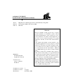
A ALBORG U NIVERSITY
I NSTITUTE OF E LECTRONIC SYSTEMS
G ROUP 948
2002
AALBORG UNIVERSITY
INSTITUTE OF ELECTRONIC SYSTEMS
Fredrik Bajersvej 7
T ITLE :
P ERIOD :
G ROUP :
DK-9220 AALBORG ØST
High Precision Tracking System For Virtual Reality Using GPS
01 September 2002 to 03 January 2003
GPS 948
Abstract
The key elements of this project was to investigate the dynamics of a kinematic system, and the
real-time determination of the systems pose (position & orientation). To direct our investigations, we
choosed to focus on the development of a specific
application. For this, we chose the virtual environment.
Some virtual environment systems require a spatial tracking application for pose purposes. Several
methods are currently used such as magnetic trackers etc. However, most of these systems only work
in a restricted laboratorial environment. With the
use of GPS technology, an outdoor system could be
made.
For such a system, the orientation and position is
rather critical, and if there is a lag between head
movement and visual feedback, the user perceives
a temporal distortions effect. It is therefore necessary to develop a system that includes a predictive
filtering techniques such as the Kalman Filter.
Real-Time Kinematic (RTK) GPS is used for the estimation of the user’s position in the virtual environment. The problems concerning system orientation
was not addressed in this project.
M EMBERS :
Tue Kluas Kyndal
Stephen N Asamoah
S UPERVISORS :
Lars G. Johansen
Kai Borre
N UMBER OF COPIES :
N UMBER OF PAGES :
H ANDED IN :
5
67 pages
03 January 2003
Preface
This report is the documentation of a 9th semester project at AAU, Institute of Electronic Systems. The project aimed at implementing a tracking system for virtual
environment. The first few chapters give a brief introduction into the requirement
of the VR system and a detailed analysis of the algorithm used in implementation.
The remaining chapters give a description of the system, test and result.
Most of the coding was done in Matlab and a lot of m-files already done by
Kai Borre was used with little modification. Few C-MEX files were also used in
reading binary data from the com ports. All the m-files mentioned in the report
together with the manual of the JPS receiver can be found on the attached CD or
the url.
• http://kom.auc.dk/group/02gr948/Projects.html
• http://tue.kyndal.dk/Projects.html
• http://uk.geocities.com/sasamoah/Projects.html
To run a test programme off-line, just type ” rtk” at the matlab command
prompt and enter. Then choice off-line mode.
Tue Klaus Kyndal
Stephen Neuman Asamoah
Contents
1 Introduction
1.1 Background . . . . . . . . . . . . . . . .
1.2 Tracking requirement in VR . . . . . . .
1.2.1 Requirements in a outdoor VR . .
1.3 Problem formulation . . . . . . . . . . .
1.4 Objectives . . . . . . . . . . . . . . . . .
1.4.1 The current project . . . . . . . .
1.5 System platform and computing language
1.6 Hardware limitations . . . . . . . . . . .
1.7 Expectations for the system . . . . . . . .
.
.
.
.
.
.
.
.
.
1
1
2
3
4
5
5
6
6
7
2 RTK systems
2.1 Introduction to RTK systems . . . . . . . . . . . . . . . . . . . .
8
8
.
.
.
.
.
.
.
.
.
.
.
.
.
.
.
.
.
.
.
.
.
.
.
.
.
.
.
.
.
.
.
.
.
.
.
.
.
.
.
.
.
.
.
.
.
.
.
.
.
.
.
.
.
.
.
.
.
.
.
.
.
.
.
3 Global Position Systems
3.1 GPS principles . . . . . . . . . . . . . . . . . . . . .
3.2 GPS observables . . . . . . . . . . . . . . . . . . . .
3.2.1 Code measurements (Pseudorange) . . . . . .
3.2.2 Carrier phase measurement . . . . . . . . . . .
3.3 GPS errors . . . . . . . . . . . . . . . . . . . . . . . .
3.4 Satellite clock & Ephemeris error . . . . . . . . . . . .
3.4.1 Ionospheric Delay . . . . . . . . . . . . . . .
3.4.2 Tropospheric Delay . . . . . . . . . . . . . . .
3.4.3 Receiver Noise . . . . . . . . . . . . . . . . .
3.4.4 Multipath . . . . . . . . . . . . . . . . . . . .
3.5 Relative Positioning . . . . . . . . . . . . . . . . . . .
3.5.1 Single-difference . . . . . . . . . . . . . . . .
3.5.2 Double-difference . . . . . . . . . . . . . . .
3.5.3 Triple-difference . . . . . . . . . . . . . . . .
3.5.4 Combination of Code and Phase Measurements
3.5.5 Baseline Vector Estimation . . . . . . . . . . .
i
.
.
.
.
.
.
.
.
.
.
.
.
.
.
.
.
.
.
.
.
.
.
.
.
.
.
.
.
.
.
.
.
.
.
.
.
.
.
.
.
.
.
.
.
.
.
.
.
.
.
.
.
.
.
.
.
.
.
.
.
.
.
.
.
.
.
.
.
.
.
.
.
.
.
.
.
.
.
.
.
.
.
.
.
.
.
.
.
.
.
.
.
.
.
.
.
.
.
.
.
.
.
.
.
.
.
.
.
.
.
.
.
.
.
.
.
.
.
.
.
.
.
.
.
.
.
.
.
.
.
.
.
.
.
.
.
.
.
.
.
.
11
11
13
14
15
15
15
16
16
16
16
17
18
18
19
20
21
4 Ambiguity Estimation Concepts
4.1 Ambiguities in Topcon receivers(what is the relevance of this sec)
4.2 Float solution . . . . . . . . . . . . . . . . . . . . . . . . . . . .
4.2.1 The variance-covariance on the float solution . . . . . . .
4.2.2 LAMBDA . . . . . . . . . . . . . . . . . . . . . . . . .
4.2.3 De-correlation of ambiguities . . . . . . . . . . . . . . .
4.2.4 The search method . . . . . . . . . . . . . . . . . . . . .
4.2.5 Summarizing LAMBDA . . . . . . . . . . . . . . . . . .
4.3 Goad Method . . . . . . . . . . . . . . . . . . . . . . . . . . . .
4.3.1 Properties of the wide lane combination . . . . . . . . . .
4.3.2 Goad’s integer estimation . . . . . . . . . . . . . . . . .
4.3.3 Evaluating the Goad method . . . . . . . . . . . . . . . .
4.3.4 Choice of integer solution . . . . . . . . . . . . . . . . .
4.4 Cycle-slip check and repair . . . . . . . . . . . . . . . . . . . . .
23
23
24
25
26
27
27
28
28
28
30
30
31
31
5 Kalman Filter
5.1 Discrete-Linear Kalman Filter . . . . . . . . . .
5.2 Extended Kalman Filter . . . . . . . . . . . . . .
5.3 Implementation of EKF . . . . . . . . . . . . . .
5.3.1 Model 1 (Static) . . . . . . . . . . . . .
5.3.2 Model 2 (Kinematic) . . . . . . . . . . .
5.3.3 Filter Initialization and Tuning . . . . . .
5.3.4 Real-Time Implementation Issues of EKF
.
.
.
.
.
.
.
.
.
.
.
.
.
.
.
.
.
.
.
.
.
.
.
.
.
.
.
.
.
.
.
.
.
.
.
.
.
.
.
.
.
.
.
.
.
.
.
.
.
.
.
.
.
.
.
.
.
.
.
.
.
.
.
33
34
35
36
37
38
38
39
6 System Description
6.1 Hardware . . . . . . . . . . . . . . . . . . . . .
6.1.1 PC and Application Platform . . . . . . .
6.1.2 GPS Receivers . . . . . . . . . . . . . .
6.1.3 Data Link . . . . . . . . . . . . . . . . .
6.1.4 Hardware test . . . . . . . . . . . . . . .
6.2 Application Software Design . . . . . . . . . . .
6.2.1 System design . . . . . . . . . . . . . .
6.3 Checks and safe procedures . . . . . . . . . . . .
6.4 Data Handling . . . . . . . . . . . . . . . . . . .
6.5 Data processing . . . . . . . . . . . . . . . . . .
6.6 Important system functions . . . . . . . . . . . .
6.6.1 GPS time, Reciever time and check time .
6.6.2 GPS ephemerides . . . . . . . . . . . . .
6.6.3 Pre-computation and check of variables .
6.6.4 Master receiver position . . . . . . . . .
6.6.5 Ambiguity estimation . . . . . . . . . .
6.6.6 The extended kalman filter . . . . . . . .
.
.
.
.
.
.
.
.
.
.
.
.
.
.
.
.
.
.
.
.
.
.
.
.
.
.
.
.
.
.
.
.
.
.
.
.
.
.
.
.
.
.
.
.
.
.
.
.
.
.
.
.
.
.
.
.
.
.
.
.
.
.
.
.
.
.
.
.
.
.
.
.
.
.
.
.
.
.
.
.
.
.
.
.
.
.
.
.
.
.
.
.
.
.
.
.
.
.
.
.
.
.
.
.
.
.
.
.
.
.
.
.
.
.
.
.
.
.
.
.
.
.
.
.
.
.
.
.
.
.
.
.
.
.
.
.
.
.
.
.
.
.
.
.
.
.
.
.
.
.
.
.
.
40
40
41
42
44
45
46
46
49
50
52
54
54
54
55
55
55
57
ii
7 System test and Conclusion
7.1 System Speed . . . . . . . . . .
7.1.1 Process speed . . . . . .
7.1.2 Receiver output rate . .
7.1.3 Modem transmission rate
7.2 Filter performance . . . . . . .
.
.
.
.
.
.
.
.
.
.
.
.
.
.
.
.
.
.
.
.
.
.
.
.
.
.
.
.
.
.
.
.
.
.
.
.
.
.
.
.
.
.
.
.
.
.
.
.
.
.
.
.
.
.
.
.
.
.
.
.
.
.
.
.
.
.
.
.
.
.
.
.
.
.
.
.
.
.
.
.
.
.
.
.
.
.
.
.
.
.
61
61
61
62
62
63
8 Conclusion
65
A Kinematic test
67
B The full ephemerids struct used
73
Bibliography
I
iii
Chapter 1
Introduction
1.1 Background
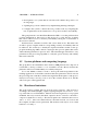
Virtual Reality is a technology that tries to mimic the real world or an immersion
in 3-D visual world. The basic idea is to immerse a user inside an imaginary, computer generated virtual world. For the immersion to appear realistic, the virtual
reality system should be able to accurately sense the users movement and what
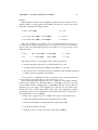
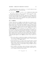
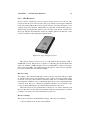
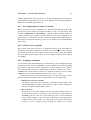
effect it would have on the scene being rendered. Usually, stereo images are projected onto two miniature screens and with the help of a Head Mounted Display
(HMD) device, one could experience fascinating 3-D objects.
Figure 1.1: Head Mounted Display
For this technology to work, means of position and motion tracking is needed.
One commonly used method in tracking position and orientation is by magnetic
1
CHAPTER 1. INTRODUCTION
2
sensors, such as inertial boxes, sonic discs, and potentiometers [Val02]. This is
needed to instruct the graphics system in virtual reality setup to render a view of
the world from the users new view point. Tracking the position and motion of the
user in virtual reality has been a topic for major research projects. And this is the
focus of this project.
Virtual Reality can be made indoors as well as outdoors. An example of an
indoor VR is a Cave Automatic Virtual Environment (CAVE), in which illusion of
fascinating 3-D objects are generated by projecting stereo images on the walls and
floor of the room with library software linking all elements. The user is free to
walk anywhere within the room wearing stereo glasses and means of head tracking
equipment.
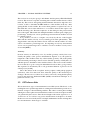
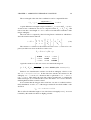
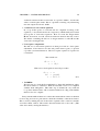
An example of an outdoor VR is Augmented Reality. In augmented reality the
user can see the real world around him with computer graphics superimposed on it.
This make it looks like both the real world and the virtual world coexist. This can
normally be used in a historical site, museums, training etc. In augmented reality
the virtual world supplements the real world rather than replacing it.
Figure 1.2: Augmented Reality
1.2 Tracking requirement in VR
Virtual Reality (VR) is defined as ”a computer generated, interactive, three-dimensional
environment in which a person is immersed” [AB92]. For the user to effectively
interact with this virtual world, real time response from the system is required. As
earlier stated in the previous section, accurate means of tracking the position and
orientation of the user is needed in order to determine the user’s view point. This is
then communicated to the graphics system of VR and appropriate images or scenes
are then rendered and sent to the Head Mounted Device/Display (HMD). Usually
24 - 30 frames per second are needed, to experience a good visual effect [Soc02].
This update rate gives the basic requirements for the tracking system, since every
frame is computed as a function of position and orientation.
CHAPTER 1. INTRODUCTION
3
Current technologies for head tracking systems make use of magnetic trackers
or audio systems with an update rate of about 180Hz [Soc02]. These system must
be set up and configured in a restricted environment, because the use of magnetic
trackers introduce errors caused by metal objects in the surroundings. Likewise
the audio systems can be confused by echoe’s. These errors appear as errors in
position and orientation and can not easily be modelled. The range of such a tracking system are also rather limited (approximately 25m) . If the range is exceeded
or the update rate is slowed down, lags between the position and orientation estimation and the rendering device could occur, giving the user a temporal distortion
experience [Soc02].
1.2.1
Requirements in a outdoor VR
To move the VR outdoor, which is the purpose of this project, other approaches are
needed to govern tracking of the system. This requires a tracking technology that
could work outdoor without a large hardware setup, and independent of time and
place.
The specifications for an outdoor system, differ from the cave system, given the
different circumstances. Most important is the distance to the augmented object,
that normally is assumed to be much longer than in the cave. An example could be
a session where a new windmill has to be visualized to the public.
The longer distance means that a bias on the position is less significant, because
a offset is impossible to distinguish, meaning that a minor bias of the position
would not matter, as long as it does not flicker to much. An approach that smoothes
the position is needed. The orientation on the other hand is a different matter. Since
an angular error of the orientation is enlarged proportional with the distance to the
object.
One way of solving the above mentioned problems would be to restrain the
users view point by using a special designed pair of binoculars, set up in a unmovable frame, so an accurate angular measurements could be preformed. This could
augment the object with great accuracy, but will not give the user a real VR experience. For this reason the system has to give up of the restrictions of a fixed set of
position and frame, and follow the user around.
It is hard to set up a final and realistic specification for such a moving VR
system, since in reality would depend on the users ability, and ”will” to accept
some distortions in the augmentation. It is a known fact that a VR system, can
cause nausia if the images flicker to much.
The system setup should be a balance between a system that automatically
restrain the users movement giving very small image variations, to a more free
system which may temporally give the user image distortions, especially at sudden
movements. In the latter case, it will be up to the user to restrain and control the
amplitude of the system movements in a degree that only give distortions that are
found acceptable.
System that is good enough, could likewise only be decided by user tests. If
CHAPTER 1. INTRODUCTION
4
the user is not capable of controlling the system in such a manner, that image
distortions can be avoided, or if the system requires major movements restrictions
to work, the system clearly is ineffective.
Still a number of minimum demands are required to obtain a system, that a user
could accept. First the position and orientation update rate, must as a minimum
follow the image update rate which is 24 − 30Hz, to enable a good augmented
image. The accuracy of the measured position must be good enough to ensure
a steady filtered position on cm level, when the system is stationary. Secondly
position filtering techniques has to ensure a quick reaction of position movements,
to enable a good tracking capability. The accuracy of the orientation measurements
and filtering, has the same characteristics. It has to settle on a steady direction
within a fraction of a degree when the system is stationary, and also quickly adjust
on sudden movements. For both position and orientation, the capability of quickly
finding a stable state, is the overall important feature. A minor bias can be accepted,
if the former is obtained.
The above discussion of outdoor VR, has given ground for the following hypothesis.
The positioning of an outdoor VR system, can be obtained by the
use of GPS measurements, and filtering techniques.
Solution of the system orientation could be done simultaneously,
but would require more equipment and other measurements.
1.3 Problem formulation
It is the aim of this project, to investigate whether or not the use of GPS technology
can be used to achieve some of the requirements of the VR system, especially
regarding the positioning of the system.
In the case where the VR environment is moved outdoor from the normal cavelike laboratory environment, a more hybrid systems are needed. Here, GPS system
could be investigated because current processing algorithm of the technology is
able to give a fast and accurate position of the user in space, nearly regardless of
time and place. Furthermore, by using hi-tech filtering technologies a filtered and
predictive update of the position can be computed. With extrapolation algorithms,
an even faster position update rate, could be achieved.
From the above discussion, the following main and subproblems has been formulated.
Main problem
How can we obtain a system position, at the update rate and accuracy required by the VR system?
CHAPTER 1. INTRODUCTION
5
Sub-problems
• What are the hardware limitations?
• Which software platform, and computing language should we chose?
• Which GPS solutions are appropriate.
• Can we improve the speed and accuracy of the GPS solutions by filtering
techniques?
• What is the optimal solution regarding measurement update rate, and computing load.
The given problems leads to a number of needed tasks that must be solved,
before a system can be developed which will meet the requirements of the VR
system.
1.4 Objectives
The obvious background for the system specification is the mentioned demands
of the VR system. Keeping in mind that it requires a position update rate of at
least 30Hz, with an accuracy less than 1cm. The project group acknowledges that
this might not be possible without additional measuring equipment like acceleration meters, inertia navigation systems (INS) or angular measuring devices. All
of which would be a natural part of the complete outdoor augmented VR system,
computing real time position and orientation. The project group have decided to
skip the system orientation, and does therefore not have the option to include outputs from the above mentioned measuring devices, in the position computation.
The specification is therefore designed to meet only the requirements of the
GPS part of the system. That means that the real VR software would get input
from the developed GPS system and a range of other sensors to achieve the much
higher VR requirements.
1.4.1
The current project
Basically, the current project would focus on tracking the position of the user’s
view point by using GPS technology. The first phase of this project would concentrate on:
• Setting up a real time Double Differential GPS system (DGPS), similar to
the Real Time Kinematic surveying systems (RTK).
• Exploring software and system platforms for the system development.
• Investigating GPS and filtering algorithms and evaluating their capabilities
in solving the stated problems.
CHAPTER 1. INTRODUCTION
6
• Development of a system that in real time will estimate the position of a
moving target.
• Updating the position estimations by implementing filtering techniques.
• Configure the system to achieve the best possible result, by comparing the
rate of update that can be obtained vis-a-vis position accuracy and stability.
The group intends to use Real-Time Kinematic GPS to solve the problem about
position determination. One aspect of this project is to verify the rate of update
that can be achieved vis-a-vis accuracy and stability, taking into consideration of
the resources at hand.
Problem about orientation would be left out for future work. The main issue
at stake is speed of update with its corresponding accuracy and stability that can
be achieved. We would try to identify the required elements needed for the appropriate tracking algorithm, and also investigate the speed of update that can be
achieved having in mind of a speed of 30Hz. The intended approach will be to vary
parameters in the processing algorithm to verify the speed, accuracy and stability
that can be achieved.
1.5 System platform and computing language
The group have both a linux/unix and a windows 2000 platform at its disposal. It
is intended to develop software so it is executable on both. Mostly because the
platforms will be tested individually, for stability and speed.
For a start Matlab software is used to develop the needed algorithm for the
tracking applications. It should be stated here that, this platform would slow down
the processing time. And this would be investigated in the first phase of the project.
It may be necessary to develop some or all of the software directly in C, but this
will not be part of the apparent task.
1.6 Hardware limitations
The group will be working with two Topcon Legacy receivers. This receiver is
according to the manual [Top01], capable of giving an update rate of 100ms. 50ms
is possible but not recommendable. This has been investigated by a test program
in Matlab, that only received and check output for the two receivers connected to
comports at baud rate 115200bps. The fastest update rate obtained in the test was
200ms or 5 Hz. After a modem had been connected between one receiver and
the computer, another test was performed. The modem could only be set to a limit
baud rate of 38400bps.
CHAPTER 1. INTRODUCTION
7
1.7 Expectations for the system
Given the above described platform possibilities, and hardware performances, the
following expectations to the system has been formulated.
• a position with a standard deviation σ of 0.3cm.
• an measurement update rate of 5Hz.
• a filtered and predicted position, capable of tracking a moving target with a
maximum speed of 0 − 5km/h and a constant acceleration.
Chapter 2
RTK systems
Before we discussed all the different GPS algorithms and filtering techniques, let
us briefly describe how it is all used in one of the most common GPS applications
namely Real Time Kinematic positing systems also called (RTK systems).
2.1 Introduction to RTK systems
The real time kinematic technique is a way to use GPS measurements which provides real time centimeter positioning. As such, it can be considered as a precision
measurement instrument which can be used by engineers, topographers, surveyors
and other professionals requiring this kind of a tool, in the same way as traditional instruments (optical or optoelectronic) are employed. Used in this mode, the
GPS offers significant advantages compared to more classical devices, especially
in terms of productivity and more relaxed operational constraints (GPS operates 24
hours a day, in any weather or visibility conditions), and can consequently, in some
cases, result in actual complete replacement of the more traditional tools altogether.
Kinematic GPS can be used not only as a simple metrology instrument, but
also as a core for navigation systems or automatic machine guidance in a variety
of application areas in civil engineering.
Technically speaking, real-time kinematic is a GPS differential mode of operation using carrier phase measurements, as such it is a technique which makes use
of the most accurate information delivered by the GPS system. The actual phase
observations taken require a preliminary ambiguity resolution before they can be
made use of. This ambiguity resolution is a crucial aspect of any kinematic system, especially in real-time where the mobiles velocity should not degrade either
the achievable positional performance or the systems overall reliability.
The RTK system setup is normally designed to overcome a given task in the
best possible way, regarding system requirements, budgets and performance specifications. Overall two different approaches are common. Either the system contains
one single GPS-receiver, and a radio or GSM link, from where special designed
differential corrections can be received. This systems require a subscription, to
8
CHAPTER 2. RTK SYSTEMS
9
receive the corrections, and offers global (note: Some systems are indeed global,
and uses satellite transmitted corrections, but the most common are restricted to
a specific area, defined by boarders or geographical features) real time centimeter positioning. These systems are often used in the industry, farming and other
commercial branches, where a reliable and fairly accurate position is needed.
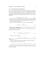
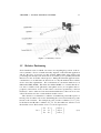
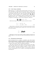
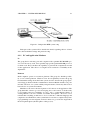
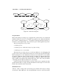
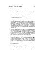
Another approach is generating the corrections within a DGPS environment.
An example is shown in the figure below. This requires a minimum of two receivers
linked by radio communication, and specially developed software, to compute the
corrections. If one of the receivers is mobile it becomes a RTK system. Such
an independent system is often more accurate than those where the corrections
are offered commercially. Mainly because the setup of the master receiver can be
done closer to the area where the rover is measuring, giving shorter baselines and
better error determination. A local system is also normally more precise because
it does not have the errors and bias introduced by a global system. This method is
often used by surveyors or entrepreneurs, needing highly accurate positions. The
downside to the system is the need of a larger system setup, which requires both
equipment, time and technical know how.
Figure 2.1: Independent DGPS system setup
Beside an overall economical evaluation, the choice of system type, depends
on the requirement of a given task, the available hardware and the know how to
use it. In this case the group has chosen to set up an independent RTK system with
CHAPTER 2. RTK SYSTEMS
10
two receivers and a radio link. The reasons for this choice are trivial. First it is
the purpose of the semester to investigate the algorithms of DGPS, and secondly a
highly accurate positioning system is needed. Secondly the group can not use any
commercially broadcasted corrections, since no agreement with any such system
has been made by the AAU GPS department.
It would be quite interesting to investigate how well the system could work,
using commercially broadcasted corrections signals. If the GPS guided VR-system
were to be produced and sold commercial, this other approach would be highly
appropriate, because it would lower overall system cost, and needed knowhow
to use it. Though such an investigation would be good for a full project alone.
Therefore the group does not intend to go into this matter.
Chapter 3
Global Position Systems
As stated in the problem formulation, we intend to investigate the possibility of
using Global Position System (GPS) to meet the tracking requirement of the virtual environment system. Other methods for tracking in the virtual environment
exist, such as magnetic trackers and sound trackers. However, the interest of the
group in using GPS stem from the background of the group members and also the
requirement for this semester. Hence we intend to concentrate on the use of GPS
technology in meeting the position requirement in the virtual environment.
Currently, there has been significant advances made in system and receiver
technologies. This advances have enhanced the effectiveness of satellite position
technologies. This chapter therefore, gives a brief description of the GPS system,
measurement techniques, errors that affects the accuracy of positioning, and mathematical modelling of the measurements.
This theoretical algorithm analysis chapter became very necessary because it
is the bases upon which our data processing are made. We discussed some of the
options available and the reason why some algorithm are preferred than others.
3.1 GPS principles
Global Position Systems (GPS) is a satellite-based system that can be said to provide a high level of positioning accuracy. It became fully operational in 1994 and
has a worldwide coverage that benefits all nation. GPS allows user with proper
equipment, mainly GPS receivers, access to useful information such as position,
velocity, and time anywhere on the globe. Determination of the position, velocity,
and time information is done by reception of the GPS signals from the satellites to
obtain ranging information as well as other necessary transmitted messages .
The system consists of four satellite at each of six 12-hour orbital planes at
altitudes of about 20200km, making up the Space Segment. Ideally, four or more
satellites is visible from anywhere in the world. Periodic update of information that
is disseminated by the satellites is done by the Control Segment. Information given
by each satellites includes satellites ephemerides, health status and constellation
11
CHAPTER 3. GLOBAL POSITION SYSTEMS
12
almanac.
Each satellites transmits a base frequency, generated by the satellite clock, on
which a number of other signal are modulated. First the two microwave carrier
frequencies with the following properties.
• Base = 10.23 MHz
λ ≈ 30m.
• L1 = 154 * 10.23 MHz = 1575.42MHz
λ ≈ 0.1905m.
• L2 = 120 * 10.23 MHz = 1227.60MHz
λ ≈ 0.1905m.
They are modulated by two binary codes: a Coarse/Acquisition (C/A) code on
L1, and a Precise (Encryted) [P(Y)] code on L1 and L2. C/A code is available to
all users. The encrypted higher precision code called Y code is reserved for only
authorized users.
• C/A
= 0.1 * 10.23 MHz = 1.023 MHz
λ ≈ 300m.
• P
=
λ ≈ 30m.
1 * 10.23 MHz
= 10.23 MHz
The signal structure of each signal consist of three components:
• A sinusoidal signal called Carrier with frequencies L1 or L2.
• A unique pseudo-random noise (PRN) called Ranging code, and
• A Navigation data, consisting of a binary coded data on the satellites ephemeris,
health, cloak bias parameters, and almanac.
For our project, a combination of these component of the signal structure will
be used. The reason for this choice is given in section ( 3.5.4).
Each satellite transmits a unique C/A code of 1023 bits, called chips, which is
repeated every millisecond. The chip width or wavelength of the C/A code chip
is about 300m and has a chipping rate of 1.023MHz. The P code has rather an
extremely long (1014 chips). The chipping rate of the P code is ten times faster
than the C/A code, and the chip width is about 30m. The significantly smaller
wavelength of the P code would therefore result in greater precision in range measurement than the C/A code [ME01].
Usually, a user segment consist of a GPS receiver whose basic function is to:
• capture the signal transmitted by the satellites that are visible,
• perform measurement of signal transit time and Doppler shift.
• decode the navigation message,
• estimate position, velocity and receiver time offset. [ME01].
CHAPTER 3. GLOBAL POSITION SYSTEMS
13
The receiver in use by the group is 20 channel dual frequency GPS+GLONASS
receiver. This receiver is capable of tracking almost all the satellites that are visible
in the sky. The receiver, after getting an initial almanac data and a rough idea of it’s
location, is able to determine the PRN numbers of the satellites in the sky. After
getting the ID of each satellite, the receiver then generates a replica C/A code. It
then shift this code in time until there is a correlation between the replica code
and the incoming code. The time required to do this shift gives the pseudo-transit
time of the signal. This transit time multiplied with the vacuum speed of light gives
pseudorange. Usually four or more pseudoranges measured from satellites are used
to compute position.
It is possible for us also to compute our velocity by the use of the Doppler
shifts and the satellite velocity vector (normally given in the ephemerides). This
doppler shift is caused by the relative motion of the user and the satellite. It’s value
can be converted into pseudorange rate. In computing our velocity, measurement
of four or more pseudorange rates to satellites, as well as satellites velocity vectors
are needed [ME01].
Accuracy
Position accuracy is affected by noise, by satellite geometry, and by bias errors.
Usually the quality of the position determination depends on (1) the spatial arrangement of the satellites in the sky, called satellite geometry, and (2) the quality
of the measured pseudoranges, known as bias. Satellite geometry actually has to do
with the spread or distribution of the satellite relative to the receiver as the satellites
moves in the sky. A good coverage in azimuth and elevation offer a good geometry.
The separation is described by the so call geometrical dilution of precision in our
earlier project [Asa02].
Errors like delays in the ionosphere and troposphere, multi-path propagation
(reflection), orbit error and clock offset, affect the quality of the measured pseudoranges. However most of these errors can be removed by using dual frequency
receiver and employing Differential-GPS (DGPS) measurement technique as explained in section ( 3.5).
3.2 GPS observables
We can derived two types of measurements from a GPS system. The first is a code
tracking known as pseudorange which is a timing measurement that provides an estimation of ranges to the transmitting satellites. The other is a carrier phase tracking
which gives relative phase measurement between the received carrier phase and the
one generated by the receiver. Since the wavelength of the carrier signal is 19cm at
L1 and 24cm at L2, it allows very precise measurements of the phase to be made.
In the next section we briefly discussed simple mathematical models relating these
two measurements to their ranges to satellites.
CHAPTER 3. GLOBAL POSITION SYSTEMS
3.2.1
14
Code measurements (Pseudorange)
Transit time is defined as the time difference between signal reception time by the
receiver clock and the transmission time at the satellite [ME01]. This quantity
is mostly measured by the GPS receivers. However, it contains bias due to atmospheric delays, multi-path etc. Hence it is a pseudo-transit time. The pseudo-transit
time multiplied by vacuum speed of light gives the pseudorange P expressed mathematically as
Pis (t) = c[ti (t) − ts (t − τ )] + εsi
(3.1)
where Pis is equal to the difference between receiver time ti at signal reception
and satellite time ts at signal transmission, multiplied by the vacuum speed of light
c. τ is the transit time or travel time of the signal from the satellite to the receiver.
εsi is the pseudorange measurement error.
Receiver clock and satellite clock can be related to GPS Time (GPST) as
ti (t) = t + δti (t)
s
t (t − τ ) = (t − τ ) + δts (t − τ )
(3.2)
where δti and δts are the clock biases in the receiver and satellite respectively
measured relative to GPST [Kap96].
Incorporating the clock biases ie equation ( 3.2) and into equation ( 3.1), the
pseudorange can now be written as:
Pis (t) = c[t + δti (t) − (t − τ ) + δts (t − τ )] + εsi
= cτ + c[δti (t) − δts (t − τ )] + εsi
(3.3)
The term cτ can be modelled as:
cτ = ρsi (t, t − τ ) + Iis + Tis
(3.4)
where ρsi (t, t − τ ) is the geometric distance between the receiver at time t and
satellite at time (t − τ ).
Iis and Tis are the delays in the ionosphere and the troposphere respectively.
The model for the pseudorange now becomes:
Pis (t) = ρsi (t, t − τ ) + Iis + Tis + c[δti (t) − δts (t − τ )] + εsi
(3.5)
The accuracy of our position estimation would however depends on how well
we are able to eliminate or compensate for most of these biases, and errors in the
measured pseudorange.
CHAPTER 3. GLOBAL POSITION SYSTEMS
3.2.2
15
Carrier phase measurement
This measurement is much more accurate than the pseudorange measurement and
would therefore give a better position estimation. The carrier phase φ si is given
as the difference between the phase φi of the receiver generated carrier signal at
the instant of reception, and the phase φs of satellite generated carrier signal at the
instant of transmission. However, only fractional carrier phase can be measured at
signal reception time, leaving an integer number N of whole cycles. The estimation
of N is the so called integer ambiguity resolution.
The carrier phase equation is given (in the absence of clock bias ) as;
φsi = φi − φs (t − τ ) + Nis + εsi
(3.6)
re-writing the above equation taking into consideration of all measurement errors,
and also writing phase as a unit of distance, we have
Φsi = ρsi − Iis + Tis + c[δti (t) − δts (t − τ )] + λ[φi (t0 ) − φs (t0 )] + λN + εsi (3.7)
Note that φ has been multiplied by the the nominal wavelength (λ) of the carrier
signal to give Φ which is in units of distance.
λ = c/fo
(3.8)
It can be seen that both the code and carrier phase measurement are corrupted
by the same error. However, the carrier phase measurement which is said to be
precise has to be resolved for integer ambiguity before the measurement can be
used for any position estimation. Determination of integer ambiguity is discussed
in Chapter ( 4).
3.3 GPS errors
Most GPS measurement are corrupted with errors which tend to affect the accuracy
of the position estimation. Errors are usually noise or bias. In this section we
attempt to discuss most of these error sources briefly.
3.4 Satellite clock & Ephemeris error
The control segment is usually responsible for the computation and updating of
satellite clock parameters and the ephemeris broadcasted by each satellite. This is
usually being done by Kalman filtering (KF) techniques. The KF model, uses the
estimation of current parameters (satellite position and clock status etc.) which are
then used to predict the future values of these parameter. This is then uploaded to
the satellite, and then broadcasted as navigation message [ME01]. However, there
are errors in both the estimation and prediction of these parameters. This errors
grows with the age of the ephemeris. And therefore, if the rate of upload to the
satellite is high the error is kept minimal.
CHAPTER 3. GLOBAL POSITION SYSTEMS
3.4.1
16
Ionospheric Delay
The ionosphere is the upper part of the earth’s atmosphere extending from a height
of about 50km to about 1000km. It contains ionized gases. GPS signals travelling
through this medium are refracted by this ionized gases. The code phase tends to
delay while the carrier phase is advanced by the same amount. This ionization is
caused by the sun’s radiation. The amount of ionized gases in the ionosphere is
determined by the intensity of the sun’s radiation. The higher the sun’s radiation
the greater the ionization, meaning ionospheric delay is greater during the day and
tends to decrease at night.
3.4.2
Tropospheric Delay
Troposphere is the part of the earth that extend to about 50km above the surface
of the earth. This part of the earth contains water vapor and dry gases mainly N 2
and O2 . GPS signals travelling through this neutral molecules are also refracted.
The elevation angle of satellite determines the path length of the signal in the troposphere: the lower the satellite the longer the path signal would travel, and the
greater the delay. The apparent effect is that, the signals are delayed depending on
the elevation angle of the satellite. This delay is common for both code and carrier
phase at L1 and L2. To estimate the tropospheric delay precisely, knowledge of
pressure, temperature and humidity along the signal path are needed. To minimize
the delay, it is recommended to exclude measurements to satellites that have low
elevation mask (e.g 15o ).
3.4.3
Receiver Noise
Measurement of the code and the carrier phase are all affected by random measurement noise. This noise is usually a white noise common to all radio frequency
radiation. The error due to receiver noise varies with the signal strength [ME01].
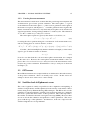
3.4.4
Multipath
GPS signals may bounce off a nearby object causing two or more signal to reach
the antenna. First the direct one and a bunch of delayed ones. The reflected delayed ones are usually weaker than the direct one. This error usually depends on
the strength of the reflected signal and delay. Both code and carrier phase measurement are affected by multipath. Improving the site of the antenna is a way of
minimizing the effect of multipath. Good antenna design can reduced multipath,
to some extend as well.
CHAPTER 3. GLOBAL POSITION SYSTEMS
17
Figure 3.1: Summary of errors
3.5 Relative Positioning
Several methods exist for which one can use in computing the position of the receiver (antenna). Choice of method usually depends on the intended application
and also the types of receivers one has at hand. Method like static single point
positioning has already been discussed in our earlier project [Asa02] and would
therefore, be left out in this current project. Taking the intended application into
consideration, we would limit our discussions on only the methods that could be
used to meet the requirements. We would therefore concentrate much more on
Differential-GPS (DGPS). The main idea behind DGPS is to assume that the errors due to satellite clock, ephemeris, atmospheric errors (ie ionosphere and troposphere), and receiver clock, are the same for receivers separated by some few
kilometers. And so when we form measurement differences, these errors are cancelled. We discussed a few of such methods in this section.
The objective is to determine coordinates of an unknown point with respect to a
known point. In other words we are determining the vector between the two points
known as the ”baseline”. For example let point A with coordinates (X A , YA , ZA )
~ be
be the known and B with coordinates XB , YB , ZB ) the unknown. And let bAB
~ can be expressed as:
the baseline vector. The baseline vector bAB




XB − X A
∆XAB

 

~
bAB =  YB − YA  =  ∆YAB 
ZB − Z A
∆ZAB
(3.9)
CHAPTER 3. GLOBAL POSITION SYSTEMS
18
If simultaneous observation are made for two satellites j and k, linear combination can be formed leading to single, double and triple-difference.
3.5.1
Single-difference
Consider a simultaneous phase observation from receivers A and B to satellites j
and k. The phase equation for the two points are:
j
ΦjA (t) = ρjA − IA
+ TAj + c[δtA (t) − δtj (t − τ )] + λ[φA (t0 ) − φj (t0 )] + λNAj + εjA
(3.10)
j
ΦjB (t) = ρjB − IB
+ TBj + c[δtB (t) − δtj (t − τ )] + λ[φB (t0 ) − φj (t0 )] + λNBj + εjB
(3.11)
As discussed earlier, if the distance between the two receivers is not too large,
the errors due to ionosphere I j , troposphere T j and the satellite clock error δtj (t −
τ ) would be similar. Taking the difference between the two observation, we have
the single difference:
j
ΦjAB (t) = ρjAB + cδtAB (t) + λφAB (t0 ) + λNAB
+ εjAB
3.5.2
(3.12)
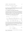
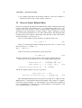
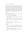
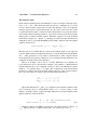
Double-difference
Consider now that observation is made to a second satellite k simultaneously, the
phase equation for this observation for another single difference would be
k
ΦkAB (t) = ρkAB + cδtAB (t) + λφAB (t0 ) + λNAB
+ εkAB
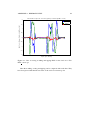
Figure 3.2: Double difference observation
(3.13)
CHAPTER 3. GLOBAL POSITION SYSTEMS
19
Taking the difference again between equation ( 3.12) and ( 3.13), which is
called the double difference , we have
jk
jk
jk
Φjk
AB (t) = ρAB + λNAB + εAB
(3.14)
Clearly, it can seen that the receiver clock bias cδtAB (t) as well as the non-zero
initial phases λφAB (t0 ) has also been cancelled. This is the reason why doubledifference is used. Note here that the cancellation became possible because we
make simultaneous observations (i.e., same time tag of epoch measurement from
both receivers), and also assumed that the measurements were made on same frequencies.
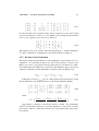
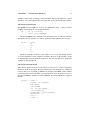
3.5.3
Triple-difference
If we now consider double-difference from two different epochs we can form the
triple-difference.
Figure 3.3: Triple Difference observation
Let t1 and t2 denote the two epochs, then from the double difference equation
we have:
jk
jk
jk
Φjk
AB (t1 ) = ρAB (t1 ) + λNAB + εAB
jk
jk
jk
Φjk
AB (t2 ) = ρAB (t2 ) + λNAB + εAB
(3.15)
subtracting one from the other, we get;
jk
jk
jk
Φjk
AB (t1 ) − ΦAB (t2 ) = ρAB (t1 ) − ρAB (t2 )
(3.16)
CHAPTER 3. GLOBAL POSITION SYSTEMS
20
The final equation for the triple-difference is then given as
jk
Φjk
AB (t12 ) = ρAB (t12 )
(3.17)
This eliminate the time independent ambiguities, the main advantage of the tripledifference. With the ambiguities cancelled, the triple difference is now insensitive
to changes in the ambiguities called cycle slips.
3.5.4
Combination of Code and Phase Measurements
So far our discussion on relative positioning has been based on measurements from
a single frequency with phase observations. We now consider measurement on L1
and L2 with both code and phase observations and then form the double difference
equations. This combination is to give an improvement in the position accuracy
by eliminating some of the errors. The setup is as shown in Figure ( 3.2). Two
receivers A and B observe two satellites j and k at the same time.
Double difference code observation equation on L1 gives:
jk
jk
jk
jk
P1,AB
= ρjk
AB + IAB + TAB − 1,AB
(3.18)
jk
jk
jk
2 jk
P2,AB
= ρjk
AB + (f1 /f2 ) IAB + TAB − 2,AB
(3.19)
and on L2 gives:
Similarly, double-difference phase observation equation on L1 and L2 gives
jk
jk
jk
jk
jk
Φjk
1,AB = ρAB − IAB + TAB + λ1 N1,AB − ε1,AB
(3.20)
jk
jk
jk
jk
2 jk
Φjk
2,AB = ρAB − (f1 /f2 ) IAB + TAB + λ2 N2,AB − ε2,AB
(3.21)
Note here that the ionospheric delay is frequency dependent hence the factor (f 1 /f2 )2
on L2. Also note the reverse sign of the ionospheric delay for the phase observation. As discussed in the previous section, on code observation, the signal is
delayed making measurement of code to long and on carrier phase, it is advanced
making measurement too short by equal amount [SB97].
Omitting subscript and superscript for all measurements, we then write the four
equations as:
P1 = ρ ∗ + I − 1
Φ 1 = ρ ∗ − I + λ 1 N1 − ε 1
∗
(3.22)
2
P2 = ρ + (f1 /f2 ) I − 2
Φ2 = ρ∗ − (f1 /f2 )2 I + λ2 N2 − ε2
where ρ∗ is the ideal pseudorange. and ε are the observation errors. Transforming
equation (1.22) into matrix form:
CHAPTER 3. GLOBAL POSITION SYSTEMS





P1
Φ1
P2
Φ2


 
 
=
 
1
1
0 0
1
−1
λ1 0
1 (f1 /f2 )2
0 0
1 −(f1 /f2 )2 0 λ2





21
ρ∗
I
N1
N2


 
 
−
 
1
ε1
2
ε2





(3.23)
For short baseline, the ionospheric delay can be assumed to be the same at both
receivers and therefore, can be set to zero [SB97]. Also putting the measurement
errors to zero, equation (1.23) can now be written as





P1
Φ1
P2
Φ2


 
 
=
 
1 0 0
1 λ1 0
1 0 0
1 0 λ2



ρ∗



  N1 

(3.24)
N2
This equation can now be solved for the ideal pseudorange ρ ∗ , and the ambiguities
N1 and N2 . Estimation of ambiguities is discussed in details in chapter 4.
3.5.5
Baseline Vector Estimation
The final step after the determination of the ambiguities is the baseline vector determination. It is intended in this project that a short baseline would be used.
Hence errors due to tropospheric and ionospheric delay are assumed to be eliminated when the double difference is formed. Double difference phase observation
equations can then be written without the ionospheric and tropospheric term.
jk
jk
jk
Φjk
q,AB = ρAB + λq Nq,AB − εq,AB
(3.25)
Setting the noise term εjk
q,AB to be zero, The equation can be linearized to obtain
the Jacobian matrix J from the derivatives of the double difference [SB97].

where




u1A − ukB
u2A − ukB
...
unA − ukB
ukA
=
k1
k1

Φk1
q,AB − λq Nq,AB − ρAB
 Φk2 − λ N k2 − ρk2
 xB
 

q q,AB
AB
  yB  =  q,AB


...
zB
kn
kn
Φkn
q,AB − λq Nq,AB − ρAB



k
k
xkECEF − xA yECEF
− yA zECEF
− zA
,
,
k
k
k
ρA
ρA
ρA
!





(3.26)
(3.27)
Approximate coordinates for the master station is needed. Also preliminary
values for the baseline estimation are needed. Equation ( 3.26) can be solved by
least square solution to obtain the baseline vector. The general least square equation is given.
CHAPTER 3. GLOBAL POSITION SYSTEMS
22
b = Ax̂
x̂ = (AAT )−1 AT b
b = A/b (In M atlab)
(3.28)
Chapter 4
Ambiguity Estimation Concepts
In the above description of DGPS, it was explained how each phase observation
equation for the double differences included an unknown integer number of ambiguities N1 and N2 , for each observed satellite. There are currently a large variety
of approaches to deal with the integer ambiguity problem, and the solution of this
equation. They are mainly divided in the following to groups; one called a float
solution, where the integer nature of the ambiguities are ignored, and the equations
are solved by means of iterative least square or filter techniques. The other is the
much more accurate fixed solution, where the correct integer number are found
mainly by the use of a search and test method, and then used in the equation solution if found valid. Another solution, which is a mixture of both, is the rather
crude round off method. Here the float solution is rounded towards the nearest integer giving one of the many possible integer solutions. This method is normally
quite bad, because of the float solution for the ambiguities Ñ1 and Ñ2 1 are highly
correlated, making a correct round off impossible. Still it is mentioned as a solution because of its fast properties, and combined with sophisticated wavelength
manipulations, it can produce a highly probable solution.
The group has no intentions of going through all the possible methods, but have
selected a few, which are found appropriate as solutions for the given problem. The
following section will therefore discuss the float solution, one of the best integer
estimation procedure called LAMBDA, and finally a round off solution in the widelane domain called the Goad’s method.
4.1 Ambiguities in Topcon receivers(what is the relevance
of this sec)
Before the different solutions are discussed, lets briefly explain the nature of the
ambiguities, and how they are treated in the Topcon receiver. The different receivers on the market all have their own way of dealing with the phase observation,
1
Ñ is used for the float solution for N
23
CHAPTER 4. AMBIGUITY ESTIMATION CONCEPTS
24
and therefore the ambiguities.
As mentioned in the DGPS theory, a phase observation is only a fraction of a
cycle of the carrier-wave. The full distance to the satellite is therefore this fraction
plus an unknown number of full ambiguities in the range of 10e 6 . This number is
impossible to measure, and have to be computed or estimated somehow.
To keep the values in this computation in a numeric stable range, the Topcon receiver uses a special trick. The fraction of the first phase measurement is
adjusted with according to the geometric range to the satellite in cycles. This produces phase-observations in the 10e6 range and integers numbers for N in the range
±50cycles, hence the deviation on the C/A code position solution.
After this fist adjustment of the phase on L1 and L2, the receiver tracks the
phase constantly and counts the number of full cycles the phase measurement is
shifted with, according to the movements of the satellite and the receiver. These
cycles are then either added or subtracted to the adjusted phase measurement in
each epoch. This means, that the unknown number of integer ambiguities always
will be the same, as long the receiver can track the phase undisturbed.
If an obstruction of the carrier or a receiver measurement error occur, the phase
tracking can easily go wrong. This causes a so called cycle-slip, and if it is not
repaired somehow, the phase measurement has a bios of one or more cycles. This
will be minimized it the position adjustment, but will always inflict an error upon
the position. Especially because the weight on the phase measurements is so high.
The method to estimate the correct number of integers, in the startup face, must
therefore be followed up some way of checking the phase measurements, and correct any cycle-slips.
It must be said, that the technology in the Topcon receiver is known to do a
good job in checking for cycle-slips and repair them it self. Newer the lees, it will
also be part of the group objective to find our own way of handling this problem.
Especially because cycle-slips have an much higher chance of occurring on a RTK
system, which moves randomly around and therefore implies many obstructions to
the carrier wave.
4.2 Float solution
Given the earlier stated double difference equations for the code and phase observation P and Φ, it was shown that the following equation could be constructed.
d = Ax − error





P1
Φ1
P2
Φ2


 
 
=
 
1
1
0 0
1
−1
λ1 0
1 (f1 /f2 )2
0 0
1 −(f1 /f2 )2 0 λ2





ρ∗
I
N1
N2


 
 
−
 
1
ε1
2
ε2





(4.1)
CHAPTER 4. AMBIGUITY ESTIMATION CONCEPTS
25
The given observation equation can be solved by means of least square. Since
two different measurements with different accuracies are included, a weight matrix
C must be introduced, before the float solution can be computed.
The weight matrix
First it is assumed that the 4 observations P1 , P2 , Φ1 , Φ2 are un-correlated. Next
the accuracy relation between a code and a phase measurement on L1, are related
to the different chipping rate on the carrier. This relation is defined as k = 154.
Furthermore, it is assumed that the accuracy on the two code and phase observations are similar. That means that the accuracy on L2 phase measurement is
given by the accuracy on L1 times f 1/f 2.
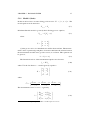
These assumptions give the following weight matrix.
C=
1
σ φ1

1
k2
 0

 0

0
0
0
0
1
1
1
(f1 /f2 )2 k2
0
0
0
0
0
0





1
(f1 /f2 )2
(4.2)
With the standard deviation on phase L1 = 0.0022 , the weight matrix look like
this.




C=
1
0.3082
0
0
0
0
1
0.0022
0
0
0
0
1
0.3952
0
0
0
0
1
0.00262





(4.3)
Having established the weight matrix C, the following least square solution to the
above observation equation can be computed.
x̂ = (AT CT )−1 AT Cd
4.2.1
(4.4)
The variance-covariance on the float solution
As a means of analyzing the quality of the float solution, the variance covariance
matrix Σx for the solution xhat , can be computed by the following equation, representing the law variance propagation for independent observations.
Σx = (AT CA)−1
(4.5)
The covariance matrix for the float solution will in this case look like this.





0.9880 −0.7465 −9.1058 −9.0701
−0.7465 0.5999
7.0683
7.0947 


−9.1058 7.0683 84.9040 84.8549 
−9.0701 7.0947 84.8549 84.8866

CHAPTER 4. AMBIGUITY ESTIMATION CONCEPTS
26
The standard deviations on the 4 un-known ρ∗ , I, Ñ1 and Ñ2 which are located
in the matrix diagonal, have the following values:
(ρ∗ , I, Ñ1 , Ñ2 ) =
q
diag(Σx ) = (0.9940m, 0.7745m, 9.2143 cycles, 9.2133 cycles)
The variances for the float solution of Ñ1 and Ñ2 , will be used for later comparison. In meters the derivations are equivalent to σN˜1 ≈ 1.75m and σN˜2 ≈ 2.25m.
Compared to the wavelength of the two carriers, this deviation is more than 9 times
one cycle. The float solution is therefore insufficient for estimation of integer ambiguities, but can be used as a first computation of the problem. Hereafter more
sophisticated methods must be implied.
4.2.2
LAMBDA
To improve the precision for DGPS, the double differences for the phase observation are often used, and preliminary a float solution is computed. To further
improve the precision, the knowledge that ambiguities always are integers can be
included in the solution. This imposes the problem of finding the correct integer
value for each ambiguity. A method for this, has been introduced by P.J.G Teunissen., and is called the LAMBDA method (Least-squares AMBiguity Decorrelation
Adjustment) [TA98].
The LAMBDA method uses an ambiguity de-correlation method, by means of
the Z-transform. Then, pairs of integers for all the ambiguities are found by a discrete search over an ellipsoidal region defined by the variance-covariance matrix,
and the correct integers are estimated by means of minimizing by least squares.
After a validation of the result, giving a ratio between the best solution and the second best, the integers are used to correct the float solution, which was computed to
establish the input argument to the LAMBDA procedure. In steps, the flow is as
follows.
• First a float solution is computed for example as described in the section
above. The float ambiguities 1 and 2 and their variance-covariance matrix Q
are used as input to the LAMBDA function.
• In the Lambda function a de-correlation is imposed on the variance-covariance
matrix Q by the Z-transform giving the de-correlated variance-covariance
matrix Z. This is then used to de-correlate the float ambiguities. Then a
search is preformed, where a selected number of integer candidates are tested
and the best pairs are found.
• After a validation of the integer solution, the integers and their variancecovariance are re-inserted into the observation-equation, and the fixed solution is computed, using the following equations.
b̌ = b̂ − Qb̂â Qâ−1 (â − ǎ)
(4.6)
CHAPTER 4. AMBIGUITY ESTIMATION CONCEPTS
Qb̌ = Qb̂ − Qb̂â Qâ−1 Qb̂â
4.2.3
27
(4.7)
De-correlation of ambiguities
If a search starting with the original ambiguities was to be preformed, it could
easily be a cumbersome process given the highly correlated state of the ambiguities.
If for instance the precision of the starting point was 1m equivalent to 11×λ1, there
would be 23 spatial candidates per double difference. With 6 satellites observed,
this would amount to 255 = 6436343 candidates to be evaluated.
Therefore a re-parameterizing known as the Z-transform is preformed before
the search is engaged. The original double difference ambiguities in the vector ~a
are de-correlated by the following equation.
z = Z∗ ∗ a
(4.8)
Where Z ∗ is defined by the Z-transformed original variance-covariance matrix
Qa by following equation
Qz = Z ∗ Qa Z
4.2.4
(4.9)
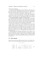
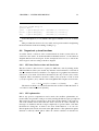
The search method
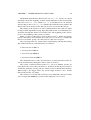
The new variance-covariance matrix Qz , can now be use to define the search ellipsoid, with which the search will be performed. The magnitude of the de-correlation
of the search space is illustrated in the 2 ellipses in the figure below.
Figure 4.1: Figure of the search ellipsoids being the de-correlated.
CHAPTER 4. AMBIGUITY ESTIMATION CONCEPTS
4.2.5
28
Summarizing LAMBDA
Given the high precision of the integer ambiguities, and therefore the fixed solution, this method is regarded as one of the better ways of solving the integer
problem. One downside to the method could be the relative heavy computing load
represented by the search and validation procedure. If the method is used only
once during the initializing process to obtain the integer ambiguities, as would be
the case in the perfect environment without cycle-slips and loss of satellite contact,
this would not be a problem. But if it has to be run often in realtime processing,
it could be a problem. How the method is behaving in realtime processing, only a
test can show.
4.3 Goad Method
The Goad method is built on a number of assumptions, which validity is the root
to the methods accuracy. The probability of these assumptions will therefore also
be the subject of discussion in this chapter.
The fact that the system layout is defined by relative short baselines means that
the ionospheric delay, can be said to cancel all together in the double difference
environment. This means that this unknown can be removed from the equation in
the float solution. If this is done the observation equation will look like this.
d = Ax − error





P1
Φ1
P2
Φ2


 
 
=
 
1 0 0
1 λ1 0
1 0 0
1 0 λ2


ρ∗





 
  N1  − 


N2
1
ε1
2
ε2





(4.10)
This assumption will hold true as long as the baseline is kept under 20 km, and
there are no intentions of making a system with baselines much over a few km all
together.
The method acknowledges that the float DD ambiguities Ñ1 and Ñ2 are strongly
correlated. The way of handling this problem is forming a linear combination of
the Ñ1 and Ñ2 also called the wide lane combination.
N˜w = Ñ1 − Ñ2
4.3.1
(4.11)
Properties of the wide lane combination
The wide lane combination can be regarded as a measurement on a simulated 3
wave, with its own properties and behavior. The most important is the wavelength,
and the fact that it is nearly un-correlated with the measurements on L1 and L2
individually.
CHAPTER 4. AMBIGUITY ESTIMATION CONCEPTS
29
The wavelength of the wide lane combination can be computed like this:
c/f1 − f2 ≈
300000000m/s
≈ 0.86m
1575M Hz − 1228M Hz
A quite different wavelength compared with the L1 ≈ 0.19m and L2 ≈ 0.24m.
A narrow lane combination can also be computed, where N˜w = Ñ1 + Ñ2 . The
narrow lane has a wavelength of ≈ 0.1m, and is not useful in the estimation of the
integer ambiguity.
The wide lane is computed by the following linear combination, which introduces the transformation matrix T.





ρ∗
ρ∗
1 0 0


 

ẑ = T x̂ =  0 1 −1   Ñ1  =  Ñ1 − Ñ2 
0 1 0
Ñ2
Ñ2
(4.12)
The variance co-variance for the transformed state vector ẑ, can now be computed, just like it was done in the float solution case.
Σz = T A−1 C −1 (T A−1 )T
0.9880 −0.0356 −9.1058


0.0490 
Σz =  −0.0356 0.0807
−9.1058 0.0490 84.9040


Again the variances for the state vector are found in the diagonal.
(ρ∗ , I, N˜w , Ñ2 ) =
q
diag(Σx ) = (0.9940m, 0.2841 cycles, 9.2143cycles)
Earlier it was found that the variance for the float ambiguity solution on L1
was σN˜1 ≈ 9.2cycles or 1.75m. In the wide lane domain, the variance for the
ambiguity σN˜w = 0.2841cycles In meters that is equivalent to σN˜w = 0.2355 ∗
0.86 ≈ 0.25m. This makes the wide lain solution, much better to estimate the
unknown integers by a roundoff method, since the chance of a correct roundoff is
much higher than in the normal L1 band.
If we assume that the integers in the wide lane, are just as stochastic and normally distributed, as in L1, 95% of the integer estimations should be within 3 * the
deviation
σN˜w ∗ 3 = 3 ∗ 0.25m = 0.75m
This is still well within the length of one wide-lane wavelength (0.86m). A correct
roundoff by this method is therefore highly probable.
CHAPTER 4. AMBIGUITY ESTIMATION CONCEPTS
4.3.2
30
Goad’s integer estimation
When the integer Ñw is estimated in the wide lane domain, it is necessary to establish a transformation to return back from the wide lane domain, so the integers for
L1 and L2 can be found. This is done by another liner combination, that is build
77
60
= λ2
. The
on the frequency relation between L1 and L2 given like this identity λ1
∗
unknowns ρ and I, from equation ( 4.12), is eliminated. First I is removed from
the equation, because of the assumption, that the ionospheric delay cancel in the
DGPS environment. Next ρ∗ is eliminated by the above identity. The so called
ionospheric free combination, is given as the following linear combination.
60Φ 77Φ2
−
= 60N1 − 77N2
λ1
λ2
Then the following 2 roundoff in the wide lane domain are executed.
(4.13)
K1 = f loorhÑ1 − Ñ2 i
K2 = f loorh60Ñ1 − 77Ñ2 i
(4.14)
These K-values are expected to be the correct integers in the wide lane domain,
and can therefore be transformed back as integers for L1 and L2. This is done by
the following equations
60K1 − K2
17
= K1 + N̂2
N̂2 =
N̂1
(4.15)
The integers Ñ1 and Ñ2 for L1 and L2 are herby computed, and can be reinserted in equation (( 4.12)) for the float solution, and a fixed position can be computed.
4.3.3
Evaluating the Goad method
Since the method is based on a numbers of assumptions, and a final roundoff,
there are no guaranties of a correct integer estimate. No validations or test can be
performed either. Though it is highly probable that the method will produce the
correct solution for good measurements. Exactly how probable a correct solution
is, depends on the accuracy of the code and phase measurements.
The solution concept may be the optimal solution for the given system. Keeping in mind, that accurate positions estimates are needed at a high rate, meaning
that the computation load must be minimized. Whether or not this is the case,
only a test can prove. Especially the possibility of wrong roundoff’s which will
produce a measurement bias of 0.86m, will have to be investigated both analytical
and through tests.
CHAPTER 4. AMBIGUITY ESTIMATION CONCEPTS
4.3.4
31
Choice of integer solution
At this point, the group has chosen to implement both the lambda and the goad
method, in the system code. It will then be up to a number of system test, to chose
which approach is appropriate. It is all together premature, to chose a final solution,
since the filter theory has not jet been elaborated. As mentioned in the introduction,
some means of filtering techniques must be applied to the solution, for an optimal
estimate. How this is implemented will be described in the next section.
4.4 Cycle-slip check and repair
As mentioned in the earlier discussion of ambiguities in the Topcon receiver, cycleslips can and will occur in RTK systems. The group has decided not to rely on the
receivers capability to solve the problem, and will therefore elaborate the following
theory, of how to deal with the problem.
First the cycle-slip has to be detected somehow. This is done rather easily,
when both the code and phase on a carrier is available. A simple check on the
observation innovations from one epoch to another can be made. The factor of the
innovations on both code and phase should be the same for both L1 and L2. In
[SB97] it has been formulated like this.
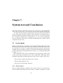
4Φ(j) = 4P (j) =⇒ 4Φ(j) − 4Φ(1) = 4P (j) − 4P (1)
To weigh down random errors and check both L1 and L2 at the same time, the
above Φ(j) and P (j) is defined as follows.
4P (j) = α1 P1 (j) + α2 P2 (j)
4Φ(j) = α1 Φ1 (j) + α2 Φ2 (j)
f12
α1 =
= 1 − α2
f12 − f22
(4.16)
This tool can be implemented as one of the measurement checks that is done
in each epoch. How to react if a cycle-slip is detected is another matter. Either the
full set of new integer ambiguities can be re-calculated, or the problem could be
fixed, by adding or subtracting the missing cycles to the now faulty integer value.
The satellite could also be left out off computation for a number of epochs, until
it is determined if the phase is regulated by the receiver itself. If it is, fixing it in
the software would cause another failure of above described test, if the receiver
at some point also repairs the problem itself. Then the newly adjusted integer
ambiguity would have to be re-adjusted back to its old value.
CHAPTER 4. AMBIGUITY ESTIMATION CONCEPTS
32
The problem of cycle-slip is therefore quite difficult, and which solution to the
problem is best, can only be decided by trying different methods and testing their
performance.
Chapter 5
Kalman Filter
In meeting the requirements of the Virtual Reality system, it is intended that realtime kinematic position update is implemented. The expected update rate that
would meet the requirement is 24-30Hz. The receiver in use is capable of updating at a stable rate of 5Hz. There is therefore the need for a predictive filtering
techniques that is capable of estimating (by use of predictor and corrector) the position of the ”user” from the available data (i.e., the 5Hz inputs from the receiver).
To explain further, a position update of at least 24Hz is required, but the receiver
in use is capable of updating at 5Hz. In between this 5Hz update rate we are to
predict the position for a few Hz until new epoch of measurement data is received
from the receiver.
Hence a Kalman Filter (KF) is being used in estimating and predicting the
position of the dynamic user in VR. The preference of Kalman filter to other filters
is because of the following reasons:
• Kalman filter make use of all measurement data available, and with prior
knowledge about the system and measurement device, it produce an estimate
of position in such a way that the error is minimized statistically.
• Apart from it being used as an estimator, the kalman filter can be used in
analysing the system error
• It’s recursive nature (which is explain later) make it a good tool for real-time
applications.
A Kalman Filter is an optimal recursive data processing algorithm. Optimal,
in that it make use of all information that can be provided to it, and recursive
because storage of previous data is not necessary. According to (Maybeck, Peter
S), Kalman filter uses
• knowledge of the system and measurement device dynamics,
• the statistical description of the system noise, measurement errors, and uncertainty in the dynamics model, and
33
CHAPTER 5. KALMAN FILTER
34
• any available information about initial conditions of the state variables, to
estimate the current value of the variables of interest.
5.1 Discrete-Linear Kalman Filter
One basic assumptions that the discrete Kalman filter makes is that the model must
be linear, and when non-linearities exist, a good engineering approach is to linearize it about some trajectory. This is because linear system are more easily
manipulated with engineering tools than nonlinear. Other assumptions are that
the system and measurement noises are white and Gaussian. This make the filter
tractable and gives the engineer a knowledge of the first and second order statistics
(mean and variance) of a noise process.
Given a system which can be modelled by an equation in the form
(5.1)
xk+1 = Fk xk + k
where Fk is the transition matrix relating the previous state xk at time k and
the current state xk+1 at time k + 1,
and k ∼ N (0, Σ,k ).
And an observations (measurements) equation given by:
(5.2)
bk = Hk xk + ek
The basic equations that forms the engine of the recursive kalman filter are:
The measurement (also known as corrector) update equations given by,
Kalman Gain Kk = Pk− HkT (Hk Pk− HkT + Rk )−1
State estimate x̂k = x̂− + Kk (bk − Hk x̂− )
Covariance of state estimate Pk = (I −
(5.3)
Kk Hk )Pk−
and the time update equations (predictor) given by;
State predict x̂−
k+1 = Fk x̂
−
Covariance of state predict Pk+1
= Fk Pk FkT + Qk
(5.4)
The element that minimizes the mean square error in the above equations is the
Kalman gain Kk . All terms have their usual meanings. The sequence of computational step is shown in Figure 5.1. Once the filter loop is entered, the computation
can go on indefinitely. To enter the loop, an initial estimate of state predict x̂ −
0 and
−
it’s covariance matrix P0 are needed.
CHAPTER 5. KALMAN FILTER
35
Initialization
Compute Kalman
Gain
Compute State
Predict and it’s Error
Covariance
Input Measurements
Matrix
Update State
Estimates
Compute Error
Covariance of
State Updates
Output State
Figure 5.1: Kalman Filter Loop
5.2 Extended Kalman Filter
The kalman filter can also be used in situation where the system is not linear. The
approach is to linearized the system process and/or the measurement process about
some nominal trajectory. Different ways exist by which this linearization can be
done. If the linearization is done about the current mean and covariance, the resulting filter is call extended kalman filter EKF [BH85]. For the EKF given the state
space equations
xk+1 = f (xk , uk , vk )
(5.5)
yk = h(xk , wk )
(5.6)
The inputs needed are the linearized state and observation equations given by;
xk+1 ≈ f (x̂k , uk , v̄k ) + A(k)(xk − x̂k ) + F (k)(vk − v̄k )
yk ≈ h(x̄k , w¯k ) + C(k)(xk − x̄k ) + G(k)(wk − w̄k )
where
A(k) =
F (k) =
C(k) =
G(k) =
δf (x, uk , v̄k )
|x=x̄k
δx
δf (x̂k , uk , v)
|v=v̄k
δv
δg(x, w̄k )
|x=x̂k
δx
δg(x̂k , w)
|w=w̄k
δw
CHAPTER 5. KALMAN FILTER
36
The error covariance matrices associated with the equations above
Q = E{uk uTk }
R = E{wk wkT }
Initial estimates of state and covariance matrix
x¯0 = E{x0 }
P0 = E{(x0 − x¯0 )(x0 − x¯0 )T }
The computational step is the same as the ordinary kalman filters and can show
by Figure 5.2.
Time update
(1) Project the state ahead
(2) Project the error covar−
iance ahead
Measurement update
(1) Compute the Kalman gain
(2) Update estimates with
measurements
(3) Update the error covariance
Initial estimates for state
and error covariance
Figure 5.2: Extended Kalman Filter Loop
5.3 Implementation of EKF
It is worth discussing how we are using EKF in estimating the position of the user
in VR by use of GPS measurement. In this particular project, two models were
implemented and both will be discussed below. Model 1 is a static receiver where
the present estimates at time k + 1 are expected to be the same as the previous
estimate at time k. The second model assumes a constant velocity and acceleration.
Hence the present estimates at time k + 1 are definitely going to differ from the
previous estimates at time k. We now go into detail description of the two models.
CHAPTER 5. KALMAN FILTER
5.3.1
37
Model 1 (Static)
In this model we have our states being position vector Xk = [xk , yk , zk ]T . The
model equation can be derived as
(5.7)
Xk+1 = Xk
In kalman filter this model is govern by the following process equation,
(5.8)
Xk+1 = Fk Xk + Q
where


1 0 0


F = 0 1 0 
0 0 1
Q is the process noise, it’s initialization would be discussed later. The measurement consist of pseudorange and phase observation and hence the relation between
the measurements and the states (position vector) is not linear. This equation can
be given as,
bk = h(xk , wk )
(5.9)
The linearized version of the measurement equation now becomes,
(5.10)
bk = HXk
where H is the Jacobian 2n × 3 matrix given by equation




H=
where
ukA
=
u1A − ukB
u2A − ukB
...
unA − ukB
1





(5.11)
k
k
xkECEF − xA yECEF
− yA zECEF
− zA
,
,
k
k
k
ρA
ρA
ρA
!
The measurement vector b is a 2n × 1 given by,
k1
Φk1
q,AB − λq Nq,AB
 Φk2 − λ N k2

q q,AB
b =  q,AB

...
kn
Φkn
q,AB − λq Nq,AB

1





Note here that the superscripts are satellites, and subscripts are receivers
(5.12)
CHAPTER 5. KALMAN FILTER
5.3.2
38
Model 2 (Kinematic)
In model two we have our states being the position vector, velocity vector, and
acceleration vector Xk = [xk , yk , zk , x˙k , y˙k , z˙k , x¨k , y¨k , z¨k ]T . This model can be
represented mathematically by the equation,
∆t2
x¨k
2
∆t2
yk+1 = yk + ∆ty˙k +
y¨k
2
∆t2
z¨k
zk+1 = zk + ∆tz˙k +
2
xk+1 = xk + ∆tx˙k +
(5.13)
The relation between the previous states and and current states are govern by
the transition matrix,








F =







1
0
0
0
0
0
0
0
0
0
1
0
0
0
0
0
0
0
0 ∆t 0
0 ∆t2 /2
0
0
2
0 0 ∆t 0
0
∆t /2
0
1 0
0 ∆t
0
0
∆t2 /2
0 1
0
0
∆t
0
0
0 0
1
0
0
∆t
0
0 0
0
1
0
0
∆t
0 0
0
0
1
0
0
0 0
0
0
0
1
0
0 0
0
0
0
0
1
















In this model the H matrix is the same as model 1 only that it is expanded with
zeros to take care of velocity and acceleration vectors. H matrix in model 2 now
becomes a 2n × 9 matrix. Observation vector b is however the same as model 1.
5.3.3
Filter Initialization and Tuning
In both models the parameters used in initializing the filters are the same. The only
difference is the sizes of the matrix which are changed to reflect the state estimates.
The states estimates were initialized to zeros in both cases.
The measurement noise covariance R was measured prior to operation of filter.
This was done by taking the variance of measurements . Choice of process noise
covariance Q was quiet difficult because we do not have the ability to directly
observe the process we are estimating. A better approach would have been to
change Q dynamically during the filtering process by use of mathematical model.
But time limit could not permit modelling of a random walk. In our case where we
are tracking the head of the user in virtual environment, it would have been good
to reduce the magnitude of Q as the user stand still, and increase the magnitude as
he start moving.
CHAPTER 5. KALMAN FILTER
5.3.4
39
Real-Time Implementation Issues of EKF
As have been said in the previous discursion, the recursive nature of Kalman filter
makes it suitable for real-time applications. This is because there’s no need of
storage of previous data used in computation, therefore taking less time for the filter
to execute. However, there is some kind of processing and transmission delays that
should be addressed. This is the time when measurement data becomes available
and the time, data is passed on to the filter. Also a delay between Kalman filter
computation time and time of data output to the needed place. One way of going
about this problem is to make a projection of the Kalman filter so that solution are
delivered the VR system. The danger here is that there is the likelihood that error
covariance associated with the solution could be corrupted.
Another problem worth discussing in real-time applications is the time interval
between measurement. If this time interval varies considerably or in cases where
measurement data is not available, a problem then arises on the state estimates xˆk
and error covariance Pk . One way is to predict consistently using the transition
matrix Fk and the process noise covariance Q computed for a fixed change of time
[BH85].
Chapter 6
System Description
This chapter gives a detail description of the system we have developed. The first
section describes the hardware part of the system which consist of the GPS receiver
being used, computer hardware, and the modem used as radio link. This description is very relevant in that our choice of hardware has an imposed limitation on
the performance of the RTK system. Secondly a description of the hardware component would give a better understanding of the final result obtained in the overall
system setup. The second part of this chapter describes the software developed for
processing and handling of GPS measurements.
6.1 Hardware
As discussed earlier, the group intend to make an independent RTK system, to
govern the position for the VR-application. Since we have decided only to take
GPS measurements into account, this will include two receivers, a radio link and
a PC. The system setup is shown in the figure below. In this section, the selected
hardware is briefly described, and system specific settings if any are listed and
explained.
40
CHAPTER 6. SYSTEM DESCRIPTION
41
Figure 6.1: Independent RTK system setup
Each part of the system will be described in detail, regarding choices of hardware, their individual settings and practical setup.
6.1.1
PC and Application Platform
Pc
The group had a stationary personal computer with a pentium III 700 MHz processor for laboratory work, and a portable laptop with a pentium III 600 processor
for field work. They both have the capability to perform the computations needed
for the application. The choice of computer were restricted to availability at the
department.
Platform
Both computers operate on a windows platform. The group also had the possibility to use a Linux platform. Windows were chosen primarily because the group
has limited knowledge about the Linux system, and also because the group experienced large problems with the communication between Matlab and the com ports
in Linux. However, for system stability and performance, Linux may have been a
better choice of system environment.
Matlab was chosen for the development of all software to the application. The
group finds this software good for developing new code because of all the ready
to use features and easy readability of codes. Also a comprehensive library of
existing Matlab code were available for further development. However, it was
realized that everything would have to be re-coded into a different language and
compiled as executable files, if the system had to be used in a complete VR system.
C programming were investigated, and was found to be good, but was neglected in
the development phase (the first phase of this project).
CHAPTER 6. SYSTEM DESCRIPTION
6.1.2
42
GPS Receivers
From a variety of different receivers, Topcon Legacy receiver was chosen. The
reason for this choice was first because the group wanted to investigate a different
receiver from the Ashtech that were used last semester. Secondly, the legacy is very
compact and power efficient, which makes it preferable for kinematic purposes.
After having investigated the manual, it also became clear, that it could provide
the group with the measurements needed at a higher update rate than any of the
receivers available in the department at the moment.
Figure 6.2: Topcon Legacy receiver
The Topcon Legacy receiver in use is a 20 channel dual frequency GPS +
GLONASS receiver. The receiver is capable of outputting raw measurement data
at the rate of 50 ms or 20Hz, though it is not recommendable to query for measurements faster that 10Hz. Any further detailed description of the receivers capabilities can be found in the user manual [Top01].
Receiver setup
According to the manual [Top01] the receiver can be connected with up to 30m
of antenna cable before any amplifying of the signal is needed, and the cables
used were only 15 m. The extension of antenna cable, does not influence the GPS
measurements, which also were confirmed by the Topcon service department when
contacted about the topic. Therefore permanent antennas were installed on the
rooftop, making GPS signals accessible in the department’s laboratory.
The master receiver were permanently connected to one of these antennas, and
the rover the other for stationary measurements in the development phase. Another
portable rover setup were used for kinematic system tests.
Receiver settings
The receivers used the standard/default settings, with only a few changes.
• Power standby mode if idle, were disabled
CHAPTER 6. SYSTEM DESCRIPTION
43
• The GLONASS satellite system was disabled
• The internal measurement rate were set to 100 ms or 10 Hz
• The com port baud-rate were set to 38400 bps
The power standby mode were disabled, so the master would not shut down if
idle during tests. Secondly when both the master and the rover were connected to
the pc in the laboratory, the receivers could at anytime be reached by contacting
the pc through the internet. This feature gave great flexibility for running system
test from our own pc’s at home.
Since the system were intended to operate on the GPS system alone, the Russian GLONASS system were disabled. Implementing GLONASS into the system,
would also go far beyond the project scope.
When setting the internal measurement rate from the default value of 200ms to
100ms, all measurement output rates in multiples of 100ms are made possible. At
this point the actual output rate from the GPS to the VR-system has not yet been
decided.
The comport baud-rate has to be set according to all other devices used in the
system. Here the tight point of the system is the modem used for radio link, which
will be described later. Choice of baud-rate was imposed by the workable baud-rate
in the modem.
A final but rather important remark. The time transmitted with each measured
epoch, is time of day in ms (tod) in a topcon receiver. This has to be converted into
seconds of week (sow), if this is the chosen time environment. We chose to do so,
since the ephemerids data is designed to correspond to sow. Another thing, some
receivers like Ashtech ZXtreem, correct the clock offset constantly, and outputs a
smoothed GPS time. This is different in the Topcon receiver which crudely resets
the receiver clock every time the clock offset exceeds 1ms. This is not important for
DGPS applications since the clock offset cancels, but worthy mentioning anyway.
Set and Query commands
Within the application software, a number of settings and querying were done.
These commands are all described in the GPS Interface Language (GRIL), which
is reference for detailed information [Top01]. Here only the most common commands used will be mentioned. All set commands follow the same format. The
set commands are meant to be printed to the receiver through the comport. An
example of a set-command that will reset the receiver.
General format: ”set,object name,value”
Reset command: ”set,/par/reset,yes”
The query for data output, is also a set command, that either enables or disables
a Javad Positioning Systems (JPS) output file. The handling of this file will be
CHAPTER 6. SYSTEM DESCRIPTION
44
described later. If one set of data is only needed once, it has to be enabled by
a set command properly processed and then disabled again. Otherwise the data
will be repeated with the default rate of 1s. Any number of data types can also
be enabled with a specific output rate. All the query commands follow the format
em,/cur/log,/msg/def. The list below show how the three data quarries used in the
system, are designed.
Enable/Disable Receiver Date and GPS Time
”em,,jps/RD,GT” , ”dm,,jps/RD,GT”
Enable/Disable GPS Ephemerides data
”em,,jps/GE” , ”dm,,jps/GE”
Enable chosen data measurements at rate 0.6 sec
”em,,jps/RT,SI,R1,R2,P1,P2,EE:0.6”
Disable all Measurement output
”dm”
What is actually queried for will be described in details in section ( 6.4).
6.1.3
Data Link
A radio modem, Satelline 3AS was used as a data link in kinematic setup. Detail
information about these device can be found in the user’s manual [SAT01]. The
important things relevant to this project is described below.
The maximum data speed for an RS-232 serial interface for this modem is
38400bps. This setting has to be the same for both the transmitting modem, the
receiving modem and the GPS receivers. Data format is asynchronous RS-232.
Also the link has to be a line of sight and has a range of about 20km, depending on
your antenna hight and transmit power level.
All settings of the modem was done by the program SATELLINE SaTerm version 3.1.21. To enable the program mode, the modem must be connected to the
the programs hyper terminal at baut-rate 9600 bps, and pin 12 on the comport must
be connected to ground.
Here are shown the exact modem configurations used in the project. Be advised
that the power output level was turned down to the minimum of 10 mA, when test
was performed in the laboratory, to reduce the noise level (modem antenna distance
was less that 5 m).
CHAPTER 6. SYSTEM DESCRIPTION
45
***** SATEL 3AS *****
SW Version 0.37
HW Version 01/01
-------------------------------------------------------------------------Current settings
---------------1) Radio frequency
433.0000 MHz [ CF 433.0000 MHz, Spacing 25 kHz ]
2) Radio settings
Tx Power Level 100 mW / Rx Sensitivity Level -110 dBm
3) Addressing
RX Address ON 0001 / TX Address ON 0001
4) Serial port 1
ON / 38400 / 8 bit data / None / 1 stop bit
5) Serial port 2
OFF / 19200 / 8 bit data / None / 1 stop bit [RS-232]
6) Additional setup
Error Correction OFF / Repeater Function OFF /
SL-commands OFF
7) Tests
Test Mode Unactive
8) Restore factory settings
E) Exit
Important SATEL modem issues
Because of our rather large problems with the radio modem, some issues that can
not be found in the manual are described here. Before disconnecting the modem
in programing mode, remember to push E for exit ( or Q for quit in old SATEL
versions), and then disconnect pin 12. The program session is ended and settings
are saved. Otherwise settings are not saved. Also notice that the Topcon receiver
will share its power supply with the radio modem which requires 300 mA when
transmitting. (It will appear to be working just fine, but will stop during transmission). It is therefore NOT possible to run both the receiver and the modem on
a single net-adapter. Connect therefore a fully charged battery to the secondary
power supply port on the receiver, when using the radio modem.
6.1.4
Hardware test
The complete hardware setup were tested with different settings for baud-rate and
receiver output rate. The purpose of the test were to ascertain how much we could
expect of the radio link connection. This connection test was supposed to be part
of the background for the software design. Unfortunate this test failed for all tried
settings, to our great frustration. After a point, the radio link was given up, and it
was decided to use normal comport connections to the master and rover receiver in
the laboratory.
After the software had been developed, the radio modem was investigated once
again, and a loose connection in one of the antenna cables were accidently found.
After this point the radio modems worked to some satisfaction. But unfortunate the
group had no time to investigate all the different settings once again. It was decided
to use one that worked, which is described above. A more stable connections
are assumably possible and should the setup if the modem have been investigated
further.
CHAPTER 6. SYSTEM DESCRIPTION
46
6.2 Application Software Design
This section will describe how the software has been designed, for the handling
and processing of the measured GPS data to overcome the given task. Before a
detailed description of the individual systems steps and functions, a few general
remarks about the overall design are made, and the guideline diagrams of the software design will be shown.
Some guidelines regarding the system design, to insure effective and standardized coding were made. First of all, the group wanted to make the software product,
as stable, sufficient and self explanatory as possible. The following design concepts
were listed.
• Standardized script style with explanatory comments,
• Use functions and subfunctions when possible,
• Use a predefined environment of structures and cells for data and variables,
• Make defensive coding, to prevent system crash,
• Optimize coding regarding speed and stability.
The reason for these choices are mostly to help ourself throughout the programming phase. Without a strict coding style and explanatory comments, the coding
process would get far to difficult. Secondly a predefined structure of all variables
in the system, ensured that individual developed bits of code, easily could be incorporated. Since the nature of the measurements are unstable, the programming
should be rather defensive, including a large number of checks and safe procedures
like using a ”try, catch, and end” statement. Finally the main goal is optimizing for
update speed, so unnecessary looping and computations should be avoided.
In this context it should be mentioned that, developing some of the functions
(which requires a lot of time for computation) in a C MEX file would have been
advantageous. But time limit could not permit that.
6.2.1
System design
Before we go on to any detailed descriptions of the system processes, an overall,
and rather simplified model will be explained. A selection of the most important
of the mentioned functions and script will be described in detail afterwards.
A function flow diagram were developed at the early stages of the system design, and it served as a guide throughout the system development. Hopefully it will
also give our readers an ideal of how the system is designed.
CHAPTER 6. SYSTEM DESCRIPTION
Program
mode
Get GPS Time
Get Eph
47
Basestation Position
Fix Ambiguities
Initialization
Get New
Measurement data
Fix new ambiguity
Data output
Work
loop
Extended Kalman
Filter
No
Pre−compute
variables
Che ck data
Check if
epherimedes need
update
Update
loop
Yes
Get new
epherimedes
Figure 6.3: Data Flow Diagram
Program Mode
Before the actual processing loop is engaged, the system needs to be started and
initialized. The user can choose a number of program modes, which will initialize
the system for different purposes. It should be mentioned that this interface is
meant for a development stage, and would not be part of final application product.
The following choices are possible.
• On-line process
• On-line process, with data storage for postprocessing
• Off-line process of stored data.
The main reason for these choices, are the possibility for easy debugging and
postprocessing. Notice, that whatever the choice, it is the same program and scripts
that are being run. It was deliberately decided to have both the on- and off-line
procedures within the same program, instead of making two different but nearly
similar programs for each mode. Even though it complicates things in the beginning, it makes development and testing much easier, since only a few procedures
concerning the data input are different on- and off-line.
In the following system description only the on-line mode is explained. For the
specific functionality or design of mentioned functions and scripts, we refer to the
header and comments in the actual m.file.
Initialization face:
After an ”online” startup of the system, the proper variables and comports settings
are declared. Then GPS time, date and ephemerides data are collected from the
CHAPTER 6. SYSTEM DESCRIPTION
48
GPS system. The system is now ready to handle the first real GPS measurements.
The first objective is to compute the master position, and fix the ambiguities
for both L1 and L2. This is done in a script called startup which is meant to be
executed only once, though it can be re-run if the system has to be fully reset and
started. In this procedure, a single point position of the master is found by means
of a least square solution on the code observation on L1. Then a float solution is
computed, using the code and phase observations on both L1 and l2. This solution
contains a baseline vector and float ambiguities. The float solution is then corrected
by the LAMBDA method. As mentioned the startup phase can be repeated. Eg. if
no fixed solution can be obtained within a count of 10, the system is restarted.
Work loop:
The work loop is the central part of the system, where the filtered position is computed. In short it is done by the following steps.
1. New raw data is received from the two GPS receivers. It is checked, and
processed into the struct: data(1) and data(2).
2. Common satellites for rover and master are found and all measurements are
checked for integrity.
3. Ephemerides are checked for all common satellites. If a new satellite has
appeared, or an ephemerides is too old we exit the working loop to update.
4. If all parameters are ok, we compute the position in an Extended Kalman
Filter.
5. The position is then ready for output to the VR system.
As mentioned, the work loop will be exited if an ephemerides update is needed.
Then the update loop is engaged.
Update loop:
1. First a new set of ephemerides are collected, and assigned to the struct eph.
2. Then a set of 8 unique data specimens, spaced with 2 seconds interval, are
collected. All data is checked, and must contain data from the same common
satellites.
3. This data is then feed to a least square solution algorithm, and the float solution for baseline and ambiguities are obtained.
4. This float solution is the input to the LAMBDA method, which estimates the
integers.
CHAPTER 6. SYSTEM DESCRIPTION
49
5. The baseline is corrected with the fixed integers, and the solution is feed
back to the work loop where we proceed.
The actual startup face, work and update loop all contains a large number of
functions, and scripts. It is not intended to describe all these functions, and their
algorithms. Most of them are standard GPS algorithms, like the transformation of
a baseline in ECEF coordinates into the easting, northing and upping vector ENU.
The purpose of the system description will rather be to describe how the group
managed to combine all of these function, and to describe the most important ones
like how we compute the float solution, and how the extended kalman filter works.
A very large part of the program is error checking and using safe procedures,
that keeps the system running whatever happens. We have selected the most important of these checks and safe procedures, and they will be listed and explained
in the next section.
6.3 Checks and safe procedures
When working with GPS technology, and especially real time kinematic systems,
it is important to realize the different ways one could expect system failures. We
can not state, that the system is cable of handling all possible situations, since they
are numerous. Still it has been a large part of the system development, to ensure
that the system would be cable of handling any common error situation.
Instead of going into detail, the most important ones are listed below in 3 categories. How some of the errors are corrected will not be described, since it is rather
obvious.
System checks on the common satellites used
• Check satellites for available ephemeris
• Check the age of the ephemeris
• Check satellites for fixed ambiguities
System check on raw and processed data.
• Check if the length of the raw data is correct
• Check if the raw data checksum is correct
• Check if raw data ends with line feed
• Check if any of the processed variables is NaN
• Check if the data from rover and master are in sync
• Check for cycle slips
CHAPTER 6. SYSTEM DESCRIPTION
50
Specific safe procedures
Some safe procedures are used, especially where the system is expected to crash
or stall. One example could be the control of a conditioned loop. Some algorithms
and functions uses iterations to obtain their goal, often governed by a conditioned
while, if or for loop, which could continue infinitely if not stopped. Other algorithms like a matrix invention will go wrong occasionally, with the occasionally
unstable GPS data. The following safe procedures are therefore used as much as
possible in the system. The ideal is normally just to skip the epoch, and re-try with
new data, if something turns out wrong. Some times more drastic procedures are
called for, and both function or a full system reset should be possible. Below is
listed the most common safe procedures.
• Use the try, catch, and end procedure, for all function call with an unstable
nature. For example LAMBDA which dos not always compute.
• Built in a set of default functions return values (e.g. constants, and correct
sized vectors and matrixes of zeros ), that can be returned with an error flag,
if the function does not compute.
• Use stop-counters in all conditioned iteration loops
• Use the pseudo-inverse instead of the normal inverse function, if the matrix
could be none-singular.
• Built in a reset option in the system and in functions containing changing
persistent variables, if these variables can converge to infinity or simply
misbehave.
6.4 Data Handling
In the following section, the actual data handling procedures will be described. We
start with the allocation of system variables, and measurement data.
As mentioned a predefined structure of all data arrays and variables were designed. It was decided to use structures with fields and cells, which in some cases
is equivalent to the pointers used in C-programming. Instead of handing over local
copies of large arrays with data, pointers are much faster and error safe. Another
difference between a normal array of variables and a structure with fields and cells,
is the knowledge of exactly where a specific piece of data is located. Because
the nature of the data in a GPS system, large numbers of common data is present,
therefore this knowledge is very convenient.
Data for the satellites orbits, and the measurements for a given epoch must be
locates somewhere. When using structures and fields to solve the problem, it is
possible to sort the data according to the satellite unique prn number. That means
no resources are needed to find data for a specific satellite, it would be directly
CHAPTER 6. SYSTEM DESCRIPTION
51
available, and located according to the prn number. The group defined two global
structures, one for the ephemerides data (eph) and one for the data measured (data).
Allocation of ephemerides
The global structure eph was used for all ephemerides data, so they would be
available for all function. It is designed like this.
eph = sat : [ 1 × 37 struct ]
= sateph : [ 4 5 7 9 14 24 30 ]
The fields eph.sat can contain the orbit information for 37 different satellites.
The fields however contains 21 variables picked from the ephemerides message.
eph.sat = status
sv
toc
⇓
⇓
cis
The first cell in the sat field is status. This is set to 0 or 1, depending whether
or not the ephemeris for the satellite is available. The rest of the variables are the
21 ephemerides elements defined in [Nav95]. See also the full array, with value
examples in the appendix B.
Allocation of measurements
After all raw data has been processed, it has to be allocated, so it can be reached by
the functions in the program. Because similar data measurements for 2 different
receivers has to be organized, a global 1x2 structure called data, with a number
of field and cells were used. This way measurements from the master receiver is
allocated in data(1), and the rover data in data(2). The fields in data, are organized
like this.
data(2) = nSats : 7
position : [ 4 x 1 double ]
tod : 45889
sow : 132289
usi : [ 4 5 7 9 14 24 30 ]
sat : [ 1x30struct ]
commonSats : [ 4 5 7 9 14 24 30 ]
N oComSats : 7
ref sv : 7
ref kol : 3
CHAPTER 6. SYSTEM DESCRIPTION
52
Like the eph.sat, data also has a fields called sat, where all satellite specific
data are stored according to the prn number. This fields looks like this.
data(2).sat = 1 × 30 struct
prange1
prange2
phase1
phase2
elev
To exemplified the use of these structures, lets say that the system is tracking
the 7 satellites in above examples. A call for the ephemerids status for satellite 4
would be:
eph.sat(4).status
and the measured L1 pseudorange for the same satellite would be:
data(2).sat(4)prange1
6.5 Data processing
Before the data from the receivers are processed, a data integrity check is made to
insure proper processing of the raw data. A wrong data passed on to the system
could either crash the program or give an error message. The procedure used in
checking data integrity is as follows. In the receiver user’s manual the following is
stated about the binary output massage.
All messages begin with a unique message identifier which is two ASCII characters. This is followed by the length of the message body descriptor which is
a three upper case hexadecimal digits. This descriptor gives an indication of the
length of the message in bytes. Then the message body itself follows. At the end
of every message there is a checksum [Top01].
This knowledge was used in developing the code that check the integrity of the
messages and also for parsing each message type to the correct decoding algorithm.
All the messages in an epoch has a unique identifier which is used to identify the
type of message to decipher (for example, GE for GPS ephemerides and P1 for
Code observation on L1). If any particular message is corrupt, then at least one of
the unique message identifier would be (˜ ). It is only the message containing the
receiver time RT which has (˜ ˜ ) as the identifier.
The message body descriptor (three hexadecimal digits) are decoded to get the
length of the message in bytes. The actual message is then processed and sent to it
rightful cells.
Each message body type comes in as either an integer, unsign inter, float double
etc etc, depending on the content of the messages. For example a data structure
containing the receiver date data set is given by:
CHAPTER 6. SYSTEM DESCRIPTION
struct RcvDate {
+u2 year;
+u1 month;
+u1 day;
+u1 base;
+u1 cs;
};
53
//current year [1..65534]
//current month [1..12]
//current day [1..31]
//receiver reference time [enum]
//0 - GPS
//1 - UTC USNO
//2 - GLONASS
//3 - UTC SU
//4..254 - Reserved
//checksum
where u2 is a two bytes unsign integer and u1 is just a byte of unsign integer.
In matlab, this message type could be deciphered bitwise with the fread command like this:
variable = fread(location,length,’precision’);
This was done in the initial stages of the development but it was found to be slow
reading bitwise. Also this method of processing raw data, is not very stable, and it
can be quite difficult to handle, when the length of the message is unknown. It is
also impossible to skip the full length of a corrupted massage, to jump to the next
useful massage. Therefore, another and more sophisticated method is being used
throughout out the rest of the project.
This new approach reads all the bytes available from the com port object into
matlab, and with the help of a number of special dll files developed in C ++ , we
then processed each bytes according to their precision. At typical script that would
processed all the bytes from the com port object into matlab is as follows.
while s1.BytesAvailable > 0
add = fread(s1,s1.BytesAvailable,’char’);
receph{1}=[receph{1} char(add(:)’)];
and
The above script would read everything in the com port object into matlab. The
variable receph(recorded ephemerids data) would then contain an array of all the
raw ephemerids data. This date could then be processed by a function designed
specifically for that.
Let’s for simplicity reasons reflect back to the above example showing the exact
structure of receiver date (RD). The function msgRD.m that would process this
message from a recorded data stream would then look like this. (the old way of
reading bitwise with fread is added for illustration):
CHAPTER 6. SYSTEM DESCRIPTION
54
function msgRD(msg,no)
global data
year = getu2(msg(1:2)); %fread(c,1,’uint16’);
month = getu1(msg(3));
%fread(c,1,’uint8’);
day
= getu1(msg(4));
%fread(c,1,’uint8’);
Notice the input no (1 or 2) which is the sigh for whether it is rover or master
data.
This procedure has shown to be very stable, and especial useful for deciphering
the measurements in the fast running working loop.
6.6 Important system functions
As earlier stated, a selection of the essential functions in the system will be described in some detail. To understand their individual relations, see the function
diagram that has been developed. In the description below we try to follow the
chronological order according to the flow diagram.
6.6.1
GPS time, Reciever time and check time
The first contact to the receiver is a query for GPS time, done by running m-file
GPS DateTime.m. Here year, month, day and time of measurement is collected. It
was also intended for these variables to be displayed, if a graphical user interface
(GUI) were to be made. From these informations, the day of week (dow) can be
computed. This is needed for conversion of time of day (tod) into second of week
(sow) (See equation ( 6.1)), which is done in msgRT.m that computes receiver time.
sow = check time(dow ∗ 86400 + tod/1000)
(6.1)
The function check t.m, will ensure that the time in sow is within the limits of
±302400 for numerical reasons [Nav95].
6.6.2
GPS ephemerides
Before any position computations can be made, the satellites ephemerides are
needed. They are queried for and processed by running the function gettopconeph2.m.
This script can only be executed if no other data is being printed to the comport,
and if all available data in the buffer has been collected. To ensure stability, all
massages are disabled, and the comport emptied by a special routine, each time
the function is being run. A check is also done in the function, so no error inflicted ephemerides will be allocated in the eph structure. The ephemerids update
function is called by chech eph.m, where all common satellites are checked for
CHAPTER 6. SYSTEM DESCRIPTION
55
available ephemerides. The current age of the present ephemerides is checked as
well. The limit of ephemerids age is two hours, which also is the normal ephemeris
update rate at the GPS ground stations.
6.6.3
Pre-computation and check of variables
Before any data is used for computation, we check the data integrity in the m-file
precomvar.m, and compute the common satellites for the rover and master. The
variables commonSats and NoComSats (common satellites and the number of
common satellites) are assigned as global, and used in all other computations for
index purposes. A check for cycle slips could also be implemented in this function.
The check is described in the theory section ( 4.4), but has not been implemented
at this point.
6.6.4
Master receiver position
The position of the master receiver is computed in TCrecpos ls.m. The method is
an iterative least square computation on the P code pseudorange on L1. Using the
P-code instead of the C/A code, improves the position accuracy, since the standard
deviation on this pseudorange is about 0.3 m. For further reference on the method
see [Asa02].
6.6.5
Ambiguity estimation
As described both in the DGPS theory, and in the theory about ambiguity integer
estimation, the first objective in DGSP is to make a reliable float solution regarding
the baseline components and the ambiguities for the frequencies used. This is
done in the function trkfloat.m. In this function the float solution is also feed to
LAMBDA2.m, where the fixed solution is computed my means of Least-squares
AMBiguity Decorrelation Adjustment method (see section ( 4.2.2)).
Notice that the master position already has been solved at this stage. To simplify the function description, it has been divided into the following steps.
• Find the best reference satellite
According to the theory, the best choice of reference satellite refsv, is the
one with the highest elevation. All elevations for the common satellites are
therefore computed, and the refsv selected
• Data collection
By using above described methods for data collection and data checks, 8
epochs of data from the rover and master are collected into a large data struct
ALLOBS.epoch.obs1 and obs2. Notice that all epochs of data contains the
same common satellites, so the observation equations for each epoch can be
computed in the same routine. Also the epochs are spaced in time with 2
seconds, to avoid too similar observation equations. If this is not done, the
CHAPTER 6. SYSTEM DESCRIPTION
56
variance/covariance matrix would seem ”not positive definite”, because the
values would be quite small. This is a problem occurring only when using
fast data output rate about 5-10 Hz.
• construction of observation equations
In a loop all the epochs of collected data are computed according to the
equations ( 5.12) and allocated in two large arrays, which finally will contain
all 8 epochs of observation equations. How we create the design matrix
H and observation vector b, will be described in detail in the next section.
The matrix containing the full set of design matrixes is called N and the
observation is rs(right side).
• Least square computation
The full set of observation equations are then processed in a least square
adjustment. Notice that we uses the safe pseudo-inverse (pinv), to prevent
a possible system mal-function. The least square equation is repeated for
convenience.
The normal case
H ×x = b
x̂ = H \ b
With our re-sized equations and safe procedure
N × x = rs
PP
= pinv(N )
x̂ = P P × rs
(6.2)
• LAMBDA
The next step is to feed the float ambiguities to the m-file lambda2.m, where
the fixed solution is estimated. Then float baseline vector is re-computed
with the fixed ambiguities. This entire step is included in a try catch end
loop, where default values of 0 are returned with an error flag, if the lambda
function does not compute.
Every time the rtkfloat function is called, the returned fixed solution is checked
for error flag, and a test is performed to check the reliability of the fixed solution.
This is done by making the ratio between the squared norms of the best and the
second best fixed solution. The result is discarded if the ratio is above 0.7. (This
value was found by testing the function)
CHAPTER 6. SYSTEM DESCRIPTION
6.6.6
57
The extended kalman filter
The final and most important of the function in our system is ekfrtk3.m which is
the function preparing a call to the extended kalman filter in subfunction kalman.m.
These functions will get our special attention, in the rest of this system description.
Before the actual filter routine can be launched quite a lot of preparation is
needed. The most important of this preparation will be explained in the following.
The actual filter routine has been moved to a subfunction containing the 5 filter
(see Chapter 5 ) to enhance the control of the filter.
The main purpose of the filter, is the computation of raw DGSP data into a state
vector containing the position baseline, and if chosen derivatives of this. We work
with a multiply of choices for the filter model.
• Model 1 is based on a 1 × 3 state space model. Here the state vector contains
the baseline in ECEF co-ordinates.
• Model 2 contains an example of how to include the derivatives of the state.
we include the velocity and the acceleration giving a 1 × 9 state space mode.
The filter routines are the same for both models. The only difference is the
initialization of system transition matrix F its covariance variance matrix Σ Q , and
the size of the design matrix H, and of course the state vector xˆk and its covariance/varinace matrix P.
Filter initialization
In the initialization of the function a number of variables are declared persistent.
This way the function will remember variables that are used and updated each
time the filter is called. These persistent variables are very important for the filter
routine, because they contain the information about the recursive procedure. Some
of these persistent variables will be reset and re-initialized each time the input to
the filter changes, to fit the new size of the data. Such a reset may seem a bit crude,
but it is the only thing we can do, because a re-sizing is needed when the satellite
constellation changes. This reset procedure is not regarded as a problem. E.g., The
filter covanrians/variance matrix p will converge within few epochs after a reset
to default values. The previously computed state vector xˆk is re-used as normal,
so the next new state vector will not be influenced much by this reset, since the
innovations are quite small for each epoch anyway.
The description of the function rtkekf.m will also be divided into individual
steps for simplicity.
• Ambiguity check
First the common satellites are checked for fixed solution. If any fall out,
they are removed, and will not be used in the current epoch. A flag is raised,
to ensure a re-computation of ambiguities.
CHAPTER 6. SYSTEM DESCRIPTION
58
• Check the common satellites
The next objective is to investigate how the filter should deal with the new
data set if it has changed since the last run. This is done by comparing the
satellites used since in the filter so fare, and the new set of common satellites
from the data set. The flowing scenarios could occur.
1.
2.
3.
4.
The data set contains the same satellites, as used in the filter so far.
One or more satellites has disappeared.
One or more satellites has re-appeared.
Both case 2 and 3 has occurred.
According to a case scenario test, the filter is either run with data corresponding to the previous filter setup, or the filter is re-initialized, to cope
with the new size of the new data set. A filter reset will therefore occur
serval times an hour, depending on satellite coverage and especially the constellation changes. If the system is used in a environment with meany disturbances of the satellite signal, some satellites could re- and disappear quite
often, which would re-initialize the filter each time. Still it is not regarded as
a problem, the fast update rate taken into account. The filter should be fully
converged within seconds. Though a momentary distortion of the filtered
state might occur.
• Design matrix
The design matrix H is designed according to the model and the number of
used satellites see equation ( 5.11). In this process the distance ρ to, and the
position of the satellites in ECEF is computed in the function get rho, with
the previous filtered state xˆk and the P-code pseudorangeas as input. The
satellites positions are corrected for earth rotation during the signal travel
time. The observed P-code pseudorange is used for this purpose.
• Observation Matrix
The double differences b for the observations are computed according to
equation ( 5.12). Furthermore a set of computed double differences bk is
also prepared, from the geometric distance ρ, which is the geometric range
from the two receivers at time k to all common satellites. This is later used in
the filter as the ”predicted” observations in the filtered state update equation.
• Filter routine
Finely the filter function kalman, is called. What happens in the filter, will
be described next section.
• Output
The Easting, Northing and Upping baseline ENU is computed by first transforming the rover position in ECEF onto the geoid in togeod.m. Then another transformation in the function xyz2enu, completes the job. The ENU
vector is part for the function output.
CHAPTER 6. SYSTEM DESCRIPTION
59
The kalman routine
In the function kalman.m the actual filtering is done according to the filter equations ( 5.3) - ( 5.4). The routine has been moved into a subfunction, for several
reasons. First it clarify exactly where and how the filtering is done. Secondly the
function output can be controlled better this way. If you for some reason don’t want
to update the filtered state covarinace/variance matrix P in one epoch, P could be
left out in the function return parameters. (To prevent one bad epoch destroying the
filtered state covarinace/variance matrix). The filter equations are well described
in the theory chapter (i.e., chapter 5). Though one equation in the filter has been
changed in order to cope with the DGPS measurements, and that is the state update
equation shown below.
State estimate xˆk = xˆ− + Kk (bk − Hk xˆ− )
The innovation or residuals that are scaled by the kalman gain K k are supposed
to be the difference between the measurements bk and the predicted measurements
Hk x̂− . This prediction is not possible to make because of the complex relation
in the measurement equations. Therefore a set of predicted double differences are
computed in advance and used in the filter.
Here is an example of how one set of double differences are computed, for
rover and master i and j, and reference satellites l and satellite m. Remember that
double differences has to be computed on both L1 and L2, and that the geometric
distance ρ is computed using x̂− as input. The computation of the measurement
prediction is therefore made around the current trajectory of the system, which is
the correct procedure according to the extended kalman filter theory.
lm
P1,ij
l
m
= ρli − ρm
i − ρj + ρj
lm
P2,ij
l
m
= ρli − ρm
i − ρj + ρj
The double differences P1 and P2 are computed for all satellites, and the results
are stored in the vector bk, which finally will be a 2n × 1 vector, where n is the
number of satellites. These computed double differences are used in the filter state
update equation for time k like this.
iP
State estimate xˆk
= (bk − bkk ) inovation/residual
= xˆ− + Kk (iP )
(6.3)
The final routine is the EKF is a prediction of the filtered state for time k + 1
This prediction is computed in the same way as the a prior state x̂ −
k.
x̂−
k+1 .
CHAPTER 6. SYSTEM DESCRIPTION
x̂−
k+1 = F ∗ x̂k
60
(6.4)
The prediction of the filtered state into the future, is meant to be used by another function, which would generate the 30 Hz position update needed by the VR
system. These positions are partly generated by extrapolate additional pseudo positions in between the filtered state and the prediction. This part of the system has
not been developed, since the group has realized that another and quite different
approach most likely is better. This will be discussed in the conclusion.
Chapter 7
System test and Conclusion
It has been decided to divide the system test in to categories. One regarding the
speed of the system, where we will evaluate and discuss the achievable update rate.
Secondly the filter tuning and performance will be described and evaluated.
A test of the system accuracy would have been preferable as well, but because of
problems with the radio link, time did not allow it. Also we don’t have any facilities, to establish a scientific way of tracking the rovers ”real” position in kinematic
mode. It is therefore impossible to evaluate a measured trajectory, when it can’t be
compared with a true one.
7.1 System Speed
The speed of the system, is according to the problem formulation rather critical. We
must keep in mind that an update rate of 25 - 30 Hz is needed in the VR- system.
It is currently not possible to compute GPS measurements that fast, but the faster
an update rate we can achieve, the more accurate the algorithm that extrapolate the
positions needed in between the filtered state at time k (x̂k ) and the predicted state
for time k + 1 (x̂−
k+1 ).
The output rate of the system is dependent on the performance of three parts
of the system. They are listed below in order of importance. When they all are
stretched to their limits, the final output rate of the system is equal to the slowest.
• The systems software performance, Process speed,
• The modem transmission rate,
• The receiver measurement output rate.
7.1.1
Process speed
The most important thing to optimize in the system is the process speed. Process
speed is defined as the time it takes the system to compute one update loop. If the
61
CHAPTER 7. SYSTEM TEST AND CONCLUSION
62
software process limit is 1 Hz, it does not matter how fast the receiver and radio
modem can perform, the system would jam up with data if the data input rate was
faster than the process speed.
We tested the system on both a 700 MHz and a 1000 MHz AMD processer.
Naturally the processer speed plays a critically role for the process speed. The test
was made using model 2, which clearly is the heaviest model regarding computations.
The result of the test was rather surprising. The 700 MHz, was cable of producing a process speed of 0.21 s. The 1000 MHz did much better and only used
0.08 seconds.
It should be mentioned that the process speed behaved rather strangely, on any
of the tested computers, when running for a longer period of time. At first the
process speed would settle at e.g., 0.21 s. Then the process speed would slowly
decrease to nearly a third of the initial value during the next few hundred baseline
computations to finely settle around 0.1 - 0.08 s. We don’t know why the computers tends to get that much faster when repeating the same process. The final
process speed for a given setup is therefore rather difficult to define. Since even the
slowest computer (The 600 MHz portable pc), finally settled around 0.1 s, it must
be assumed that the actual process speed is around 10 Hz, or less.
With the right computer, and further improvement of the code, a process speed
faster than 10 hz is within reach. It is important to note, that the process speed
should be a bit faster than the system update rate, leaving some time so the system
can catch up if getting behind for some reason.
7.1.2
Receiver output rate
As has been mentioned in the hardware test the receiver output rate can be expected
to be stable down to 10 Hz. This was also our experience throughout the tests, when
the receiver was connected to the pc with comport cables. Using the radio modem
is another matter. The measurement rate is therefore highly dependent of the radio
link.
7.1.3
Modem transmission rate
Since the system requires a radio modem connection, this was subject to a lot of
investigations. As has been explained a broken core in one of the cable plugs,
delayed any progress in this area till nearly the very end of the semester. Finally
the problem was solved, and we took the time to make some additional test, and
found some workable settings, which is described earlier in hardware setup.
The radio link was found to be stable when connected to a receiver with a
measurement output rate all the way down to 5 Hz, on short ranges. Power level
adjustments could properly solve the range problem.
It was also possible to use an output rate of 10 Hz, but not without several problems. First the fast output rate seemed to block the modem for incoming massages.
CHAPTER 7. SYSTEM TEST AND CONCLUSION
63
This means that when a message output has been enabled, it can not be disabled
again though the radio link. This represents a major problem with the current software designed, where the massages from the rover and master always are enabled
and disabled in sync.
With some changes of how to deal with the data from the comport object, it
may very well be possible to simply skip disabling the output message from the
receiver connected by the radio modem. One problem that might occur, would for
example be the stack overflow that could occur on the comport where the output
massage has not been disabled. This happens when the system is updating the
ephemerides on the other comport.
Anyway time does not allow us to experiment with such changes. The conclusion will have to be that an overall output rate of 10 Hz is possible, if some
problems regarding the radio link are solved.
7.2 Filter performance
In an attempt to make some form of controlled kinematic test, a method was developed where knowledge about the ”true” rover position was less significant.
Therefore a system test was performed using kinematic data from a measured
circular motion, filtered using model 2. Using a circular motion is an easy way
to investigate whether or not, the system computes the correct trajectory, just by
knowing the circle’s radius. See a description of the test in appendix A,
Filter tuning
With above described measurements, the filter was tuned in for kinematic motion.
The actual tuning of the filter parameters would be a far to big subject to describe in this report, and could easily be a full subject of its own for a 9th semester
project. Furthermore, the time in this semester was not spent on investigating the
subject in full.
The tuning was performed by testing a long set of values for the observation
and system variances used in the filter, until the filter result became reasonable.
During the tuning and filter test the following parameters were recorded for post
analysis.
• The filtered state x̂k
• Is covariance matrix Pk
• The ENU baseline
• A designed innovation vector
Plots for the final tuned filter can be found in appendix A.
The purpose of the first three items are rather obvious, since they are the direct
output of the filter. The innovation vector requires some explanation though.
CHAPTER 7. SYSTEM TEST AND CONCLUSION
64
The Kalman Gain K in the filter has the size of 9 × 2n , because it contains
information about the weighting of all the double differences in the measurements
innovation vector (bk − bkk ), which is 2n × 1. It can therefore not be analyzed
directly. The product of K ∗ (bk − bkk ), which is the actual innovation added to the
filtered state can be analysed. This innovation vector was used in the analysis.
The settings of the variances are still somewhat unclear, and could most likely
be improved through further testing. Especially with a better set of kinematic measurements. Though the discussion is still the same. The weighting of the observations vs. the weighting of the system is essential.
Either you chose a filter that is quick in the response to sudden movements,
but also vulnerable to measurement errors and noise, or you chose to configure the
filter more restricted, giving a smoother trajectory but slower response.
The following result was obtained after experimenting with the filter tuning.
The standard deviations on the different noise terms are,
• Observation noise 0,01 m
• System position 0,005 m
• System velocity 0,0005 m
• System acceleration 0,0005 m
The standard deviation of the observation noise could be derived from the observed measurement by taking the variance of the observation.
The system covarinace/variance matrix ΣQ , was more difficult, because we
really had no idea of how they should be set. It turned out that the best result was
obtained by giving the system position a variance a bit less than the measurements.
When trying to give bigger values, the system simply became too free, and the
filtered state became very jumpy.
The variances for velocity and acceleration were defined the same way. If they
were set larger than 0.0005, the system would simply run out of control.
Chapter 8
Conclusion
In giving a better conclusion for the project, it will be good to reflect on the objectives set for for this current project in section ( 1.4.1). Our focus was to implement
a tracking system for a VR system. In summary the group was to concentrate on
setting up an RTK system, and to investigate the update rate that can be achieved
in relation to accuracy and stability.
As described in chapter 6 a static and kinematic setup was implemented successfully. Hardware test was performed (see section ( 6.1.4)) which gave some
few problems with the radio link. However, after the faulty modem antenna was
detected and repaired everything worked as expected.
The next was the software test which was done by testing the main functions
in the developed software. The main functions that were tested are the function
that computes the ambiguities (LAMBDA) and the extended kalman filter where
the position vector is obtained.
The ambiguity function test was performed by running the script startup 200
times. This way the master position is recomputed and new fixed ambiguities are
estimated in each loop. For all 200 loops, the same fixed solution was found. With
the proper test routine we find the method as close to errorless as possible.
The lambda method only takes about 0.18 seconds, which is nothing compared
to the 15 - 20 seconds data collection. After final debugging the procedure also
worked to our satisfaction. The GOAD method has therefore not been implemented
or tested as we first assumed would be the case.
The next test was the kinematic test as described in Appendix A. This test
worked to some satisfaction also but time limit did not allow us to investigate further to some details. It should be stated here that, in tuning the filter we assumed a
constant velocity and acceleration. However these would not be the case in actual
implementation in the VR. Hence the system noise covariance could be determined
dynamically by some mathematical model defining the movement of the user in VR
system.
On the whole an update rate of 24Hz can be said to be attainable with some
few modification and also by making a parallel algorithm that takes an input from
65
CHAPTER 8. CONCLUSION
66
the the filter and extrapolate position in between measurement update.
The group has through the project period come to realize that using a state vector of positions, velocities and accelerations, to enable us to make a good prediction
for time k + 1, which will be used in some extrapolation routine, properly could be
done in a smarter way.
A better choice of method may have been to include a heading and heading
speed in the state vector instead. The filtered position, the heading, and its velocity, could then be used by the extrapolating routine for any period of time, until
new data arrives from the GPS system. The heading vector could also be updated
continuously with input from the much faster INS system, that is guiding the system orientation. A solution like this may both have been better to react on small
position changes, and it would definitely have been better at estimation the position
during periods, where the GPS system for some reason can not solve the position.
Prospects for the system
The future prospect for combined GPS, INS and VR system are highly dependent
of the development of hardware and their market prices. Currently the full system would become rather expensive, and the full systems would be quite a heavy
pack to carry around. The further improvement of the technologies may solve this
problem.
The prospects of actually finding any users for such a system is more difficult
to predict. Though only the fantasy can set the limits of the uses of such a system.
It may be a mandatory part of the navigating system on super-tankers in the future
for all we know, or a delightful experience of the dinosaurs when going through a
virtual theme park.
Appendix A
Kinematic test
A system test was performed using kinematic data from a measured circular motion, filtered using model 2. Using a circular motion is an easy way to investigate
whether or not, the system computes the correct trajectory, just by knowing the
circle’s radius.
Aim
The purpose with this exercise was to record a kinematic motion, which we could
compare relatively easy, to the known trajectory of the circle. Also the center point
is a good reference, because when it is re-measured after a kinematic motion, it
gives information of how fast the filtered state becomes steady again.
Procedure
A radius of 2m was used, which was controlled by a string attached to the center
point. The measurement of the circle was performed as described below.
• The center was measured accurately using a tripod
• Then one full circle was made before returning to the center for a remeasure.
• Then two further rounds were made before returning to the center to finish.
It should be mentioned that the described measured session was not executed to
our satisfaction, and if time had allowed it we would have preferred to re-measure
the session until the circle motion was executed as flawless as possible. Since we
currently only have one usable kinematic measurement this will have to do.
Results
All the results should be viewed by opening the *eps file. First because they are
in color, secondly because it helps to zoom in on the individual subplots. The
filename are included for that purpose. The files are included on the CD, and they
can be downloaded on the home page.
67
APPENDIX A. KINEMATIC TEST
68
ENU baseline Components. Test Cricle (sigmaSys = 0.005m sigmaObs = 0.01m)
2
Easting
Northing
Upping
State Vector, Changes Relative to Initial Epoch [m]
1.5
1
0.5
0
−0.5
−1
−1.5
−2
0
100
200
300
400
Epochs [0.6 s interval]
500
600
700
Figure A.1: Plot of easting, northing and upping ENU for the circle test. File:
ENU correct.eps
Here the northing, easting and upping can be compared with each other. They
have been plotted with the known center of the circle as reference point.
APPENDIX A. KINEMATIC TEST
69
Easting Vector(m)
72
25
Northing [m]
Easting [m]
71
70
69
68
67
Northing Vector(m)
26
24
23
22
0
200
400
Epoch [m]
600
21
800
0
200
Uping Vector (m)
−10.1
400
Epoch [m]
600
800
Position Vector(m)
71
Northing [m]
Uping [m]
−10.2
−10.3
−10.4
69
68
−10.5
−10.6
70
0
200
400
Epoch [m]
600
800
67
21
22
23
24
Easting [m]
25
26
Figure A.2: Plot of the individual baseline components in easting, northing, and
upping for the circle test. File: ALLENU correct.eps
The plot shows how the easting and northing making a sinusoidal motion when
a round in the circle is made. In between, they are steady at the same potion. The
plot of the upping show the antenna movement vertically throughout the test. The
actual movement has also been shown by plotting the northing in relation to the
easting. Here is clear why the group would like to re-measure the test. It clearly
could have been performed better.
APPENDIX A. KINEMATIC TEST
Statevector Position XYZ
−38
0
500
1000
0
−0.5
62
0
500
1000
0.5
0
−0.5
0
500
0.5
Z velocity
Z pos
6
5
4
1000
Y Acceleration
64
60
500
1
Y velocity
Y pos
66
0
1000
Z Acceleration
−40
X Acceleration
−36
Statevector Velocity XYZ
0.5
X velocity
X pos
−34
70
0
Statevector Acceleration XYZ
0.1
0
−0.1
0
500
1000
0
500
1000
0.2
0
−0.2
0.05
0
74
72
0
500
Epoch
1000
0.5
0
0
500
Epoch
NORM acceleration
NORM velocity
NORM pos
3
−0.5
−0.05
0
500of Position1000
0
500 of Velocity
1000
0
500
1000XYZ
Statevector
Norm
XYZ Statevector
NORM
XYZStatevector
NORM
of Acceleration
76
1
0.2
1000
0.1
0
0
500
Epoch
1000
Figure A.3: Plot of the full filtered state vector. The norms for position, velocity
and acceleration has been included. File: xF correct.eps
The plot clearly shows, how the filter finds the correct stable state in the center
of the circle, after having been in motion. How quick is not possible to tell, since
it can not be compared with any known values.
Inovations for Z (m)
Inovations for Y (m)
Inovations for X (m)
APPENDIX A. KINEMATIC TEST
71
Inovations (Kalman gain * iP) for Circle. (sigmaSys = 0.005m sigmaObs = 0.01m)
0.4
0.2
0
−0.2
−0.4
0
100
200
300
400
500
600
700
0
100
200
300
400
500
600
700
0
100
200
300
400
500
Time in epochs (sampling rate 0.6 s)
600
700
0.4
0.2
0
−0.2
−0.4
0.2
0.1
0
−0.1
−0.2
Figure A.4: Plot of the product of Kalman Gain K multiplyed with the double
difference innovations. File: ino correct.eps
Here the actual innovation vector, which is added to the a prior state, is shown
for the full test. We have only included innovations for position, since the innovations for the derivatives of the position show the same picture on a very smaller
scale. The plot clearly shows how the innovations nearly disappear when the rover
is not moving in the center of the circle.
APPENDIX A. KINEMATIC TEST
−6
variance for X (m)
8
Circle: diagonal of Co./var. matrix SxF.(sigmaSys = 0.005m sigmaObs = 0.01m)
7.5
7
6.5
5.5
variance for Y (m)
x 10
72
0
−6
x 10
100
200
300
400
500
600
700
0
−6
x 10
100
200
300
400
500
600
700
0
100
200
300
400
500
Time in epochs (sampling rate 0.6 s)
600
700
5
4.5
4
variance for Z (m)
8
7
6
5
Figure A.5: Plot of the first 3 items in diagonal of the filtered state covariance/varinace matrix P. File: SxF correct.eps
The plot shows how the variances converge form their initial values of zero, to
their final filtered values. Depending of the used variances this values converged
to differently values, but always within the very first few epochs. Using the current
set of observation, and system variances, they tend to start growing or falling a bit.
The value range in the e × 10−6 , so it is not much.
Appendix B
The full ephemerids struct used
Here an example of how the ephemerids structure looks like with real numbers
included
eph = sat : [ 1 × 37 struct ]
= sateph : [ 4 5 7 9 14 24 30 ]
The fields eph.sat, can contain the orbit information, for 37 different satellites.
The fields however contains 21 variables picked from the ephemerides message.
status
sv
toc
af 2
af 1
af 0
toe
rootA
ecc
m0
omega0
inc0
argP er
deln
omegaDot
incDot
crc
crs
cuc
cus
cic
cis
:
:
:
:
:
:
:
:
:
:
:
:
:
:
:
:
:
:
:
:
:
:
1
4
151200
0
1.81898940354586e − 012
0.000259119551628828
151200
5153.56780052185
0.00520778668578714
−0.541087018325925
0.0708340788260102
0.309338531922549
−0.551645188126713
1.34411948238267e − 009
−2.53089638135862e − 009
−3.97903932025656e − 012
268.375
−92.8125
−4.74415719509125e − 006
5.89154660701752e − 006
5.40167093276978e − 008
1.04308128356934e − 007
73
Bibliography
[AB92]
S. Aukstakalnis and D. Blatner. Silicon Mirage - The Art and Science of
Virtual Reality. Peachpit Press, 1992.
[Asa02] Kyndal T Asamoah, S. Gps monitor. Technical report, Aalborg University, 2002. Report of group 848.
[BH85]
G. Brown and P. Hwang. Introduction to Random Signals and Applied
Kalman Filtering. John Wiley and Sons, INC, 1985. ISBN: 0-47112839-2.
[Car98]
John Carnes.
Map Tools.
World Wide Web, http://www.
maptools.com/UsingUTM/UTMdetails.html, 1998. URL
visited: 24/11-2002.
[Dan02] Peter H. Dana. University of Texas; Department of Geography.
World Wide Web, http://www.colorado.edu./geography/
gcraft/notes/gps/gps_f.html, 2002. URL visited: 29/092002.
[DOF93] DOF. Interface control document - gps - 200c. Technical report, USDOF, 1993.
[Eis99]
Claus Eisenhardt. Reeltids kinematisk differentiel gps : Asip-design til
kalman filtrering. Technical report, Aalborg University, 1999. Report of
group 1028.
[GA93]
M. Grewal and A. Andrews. Kalman Filtering: Theory and Practice.
Prentice Hall, 1993. ISBN: 0-13-211335-X.
[HW97] Lichtenegger H. and Collins J. Hofmann-Wellenhof, B. Global Positioning System:Theory and Practice. Springer, 1997. ISBN: 3-211-83534-2.
[Joo01]
Peter Joosten. The lambda-method: Matlab implementation. Technical
report, Delft University of Technology, The Netherlands, 2001.
[Kap96] Editor Kaplan, Elliott D. Understanding GPS: Principles and Applications. Artech House Publishers, 1996. ISBN: 0-89006-793-7.
I
BIBLIOGRAPHY
II
[May97] Peter S. Maybeck. Stochastic Models, Estimation, and Control. Academic Press, INC, 1997.
[ME01] P. Misra and P. Enge. Global Positioning System: Signals, Measurements, and Performance. Stanford Bookstore Custom Publishing, 2001.
[Nav95] GPS Navstar. Gps-sps signal specification. Technical report, GPS Navstar, 1995. Filename: gpssps1.pdf.
[SAT01] SATEL-OY. SATELLINE-3AS, Users Guide, Version 2.1, 2001. Filename: satel manual.pdf.
[SB97]
G. Strang and K. Borre. Linear Algebra, Geodesy, and GPS. WellesleyCambridge Press, 1997. ISBN: 0-9614088-6-3.
[Soc02] Virtual Reality Society. World Wide Web, http://www.vrs.org.
uk/public/past.html, 2002. URL visited: 22/10-2002.
[TA98]
P. Teunissen and Kleusberg A. GPS for Geodesy. Springer, 1998. ISBN:
3-540-63661-7.
[Top01] Topcon. GPS Receiver Interface Language, Firmware Ver 2.2, 2001.
Filename: Grill.pdf.
[TRI02] TRIMBLE. World Wide Web, http://www.trimble.com/gps,
2002. URL visited: 20/09-2002.
[Val02]
Jim Vallino. World Wide Web, http://www.se.rit.edu/˜jrv/
research/ar/, 2002. URL visited: 20/09-2002.