Download Towards Critical Rotation - FNWI (Science) Education Service Centre

University of Amsterdam
Laboratoire Kastler Brossel
École Normale Supérieur
Master Thesis in Physics
Towards Critical Rotation
of an atomic Bose gas
Author:
Benno S. REM
Supervisors:
Dr. Kenneth J. GÜNTER
Prof. Dr. Jean DALIBARD
Dr. Robert SPREEUW
August 19, 2010
ii
Abstract
This thesis provides a theoretical basis for shaping and rotating cold Bose gases with a modulated Time-averaged Orbiting
Potential (TOP) trap. Furthermore, it documents the results our
group obtained by realising the shaping and rotating in a 87 Rb
experiment.
Our theoretical considerations are based upon a quadrupole
field superimposed by a rotating bias field - the TOP trap. By
changing the speed of rotation during a cycle, it is shown that
the average single particle potential can be shaped as an arbitrary multipod. Modulation of the rotation speed is done by
phase modulation of the currents flowing through the bias field
coils. Using this concept made it possible to obtain the average potential of the multipod up to 4th -order in spatial coordinates. Experiments confirmed the different trapping effects on
the atoms for different symmetries - different shapes of the potentials - while changing the strength of the shaping (anisotropy
strength).
Finally, these differently shaped potentials are set into rotation. Our group has investigated the influence of rotation on
the number of atoms in the trap and the theoretical predictions
done in this thesis turned out to be correct: the potential with
a 2-fold symmetry (Dipod) is not trapping at critical rotation,
whereas the potential with 4-fold symmetry (Quadpod) is. Hereby,
critical rotation is defined as the rotation frequency at which the
harmonic term of the potential is fully compensated by the centrifugal force. Measurements of the number of atoms at this frequency for different anisotropy strengths were done and compared with theoretical predictions. It turned out that the point
at which all atoms are lost, due to the trap opening up, could be
well predicted.
iii
iv
Contents
Introduction
1
2
I
1
Rotation
3
1.1
Coriolis vs. Lorentz force . . . . . . . . . . . . . . . . . . . . .
4
1.2
Hamiltonian for a particle in a harmonic potential . . . . . .
4
1.3
Critical Rotation and Lowest Landau Level . . . . . . . . . .
5
1.4
Vortices . . . . . . . . . . . . . . . .
1.4.1 Rotation of a classical fluid
1.4.2 Rotation of a quantum fluid
1.4.3 Vortex filling factor . . . . .
.
.
.
.
6
6
7
7
1.5
Potential stability . . . . . . . . . . . . . . . . . . . . . . . . .
9
.
.
.
.
.
.
.
.
.
.
.
.
.
.
.
.
.
.
.
.
.
.
.
.
.
.
.
.
.
.
.
.
.
.
.
.
.
.
.
.
.
.
.
.
.
.
.
.
.
.
.
.
.
.
.
.
Setup
11
2.1
Sequence . . . . . . . . . . . . . . . . . . . . . . . . . . . . . .
11
2.2
Time-averaged Orbiting Potential (TOP) trap . . . . . . . . .
2.2.1 Arbitrary waveform generator (Tabor WW1072) . . .
12
13
Standard TOP trap
15
3
TOP trap
17
3.1
Magnetic trapping . . . . . . . . . . . . . . . . . . . . . . . .
3.1.1 Larmor precession . . . . . . . . . . . . . . . . . . . .
3.1.2 Force due to spatial inhomogeneous magnetic field .
17
18
19
3.2
Rotating bias field . . . . . . . . . . . . . . . . . . . . . . . . .
20
3.3
Time-averaged potential . . . . . . . . . . . . . . . . . . . . .
21
3.4
Expanding the potential in spatial coordinates . . . . . . . .
22
3.5
Experiments using TOP trap to shape potentials . . . . . . .
23
v
C ONTENTS
4
Discretisation
25
4.1
Zero magnetic field points . . . . . . . . . . . . . . . . . . . .
25
4.2
Discretisation anisotropy . . . . . . . . . . . . . . . . . . . . .
27
Conclusion and Summary
II
29
Static Anisotropic TOP trap
5
6
7
31
Phase Modulation
33
5.1
Formalism . . . . . . . . . . . . . . . . . . . . . . . . . . . . .
33
5.2
Time-averaged potential . . . . . . . . . . . . . . . . . . . . .
35
5.3
Expanding the phase modulated potential . . . . . . . . . . .
36
Potential Shaping
39
6.1
Dipod . . . . . . . . . . . . . . . . . . . . . . . . . . . . . . . .
39
6.2
Tripod . . . . . . . . . . . . . . . . . . . . . . . . . . . . . . .
41
6.3
Quadpod . . . . . . . . . . . . . . . . . . . . . . . . . . . . . .
42
Anisotropy Strength
45
7.1
Discrete Phase Modulation . . . . . . . . . . . . . . . . . . . .
46
7.2
Atom losses due to a static anisotropy . . . . . . . . . . . . .
46
Conclusion and Summary
III
49
Rotating Anisotropic TOP trap
8
9
51
Co-Rotating Frame
53
8.1
53
Potential in co-rotating frame . . . . . . . . . . . . . . . . . .
Discretising Rotation
55
9.1
55
57
57
Discretisation formalism . . . . . . . . . . . . . . . . . . . . .
9.1.1 Fixed frequency resolution . . . . . . . . . . . . . . .
9.1.2 Fixed period resolution . . . . . . . . . . . . . . . . .
10 Results
59
10.1 Rotation Spectra . . . . . . . . . . . . . . . . . . . . . . . . . .
59
10.2 Anisotropy at Critical Rotation . . . . . . . . . . . . . . . . .
60
vi
C ONTENTS
Conclusion and Summary
63
Appendix
65
A Integrating Jacobi-Anger expanded functions
A.1 Jacobi-Anger expansion . . . . . . . . . . . . . . . . . . . .
A.2 Jacobi-Anger expansion for phase modulated functions . .
A.3 Multiple angle expansions . . . . . . . . . . . . . . . . . . .
A.4 Integration of a multiple angle phase modulated functions
.
.
.
.
67
67
68
68
68
B Properties of a 4th -order potential
71
C Cicero Word Generator
C.1 Tabor WW1072: Programming Standard TOP . . . . .
C.2 Magnetic Transport . . . . . . . . . . . . . . . . . . . .
C.3 Agilent N5181: Programming Evaporation Ramp . . .
C.4 Converting Interface Unit to Voltages . . . . . . . . .
C.5 Variable Timebase . . . . . . . . . . . . . . . . . . . . .
C.6 Tabor WW1072: Programming Phase Modulated TOP
C.6.1 Gated mode . . . . . . . . . . . . . . . . . . . .
C.6.2 Segmented Mode . . . . . . . . . . . . . . . . .
75
75
77
77
78
79
80
80
81
Epilog
.
.
.
.
.
.
.
.
.
.
.
.
.
.
.
.
.
.
.
.
.
.
.
.
.
.
.
.
.
.
.
.
83
Perspectives
85
Acknowledgments
87
Critical Rotation
89
Kritische rotatie
91
References
93
Index
97
vii
C ONTENTS
viii
Introduction
1
C HAPTER 1
Rotation
- Ever since the Cornell and Ketterlegroups (Anderson, Ensher, Matthews, Wieman, & Cornell, 1995; Davis
et al., 1995) in 1995 produced the first Bose-Einstein condensates
(BEC) researchers have been interested in this phase of matter. The most
stunning feature of a BEC is its phase coherence, which means that all the
particles in the condensate have the same global phase and the cloud acts
as if it is a single particle.
B
OSE -E INSTEIN CONDENSATION
Another interesting feature is the behaviour of a condensate in a rotating system, because the Hamiltonian for a particle in a rotating field is
equivalent to the Hamiltonian for a charged particle in a magnetic field.
This mean that with rotating a condensate a system of charged particles in
a strong magnetic field can be simulated (spin magnetism). Classically this
similar behaviour is seen when comparing the Coriolis force to the magnetic
Lorentz force.
When we want to look at the system of rotating a BEC the feature of
phase coherence implies that the condensate has a velocity potential described by the phase of the condensate. Which means that if there are no
singularities in the phase field the condensate can not have rotation. Feynman (Feynman, 1955) was the first to notice that in order to accommodate
rotation the condensate needed to have singularities in its phase. With his
path integral description of rotation in a condensate he could introduce
these singularities and describe them. A singularity in the global phase is
visible in a condensate as a point (tube) where the density of the condensate
is zero. These points (tubes) are referred to as vortices.
3
C HAPTER 1: R OTATION
1.1
Coriolis vs. Lorentz force
The Coriolis F C and magnetic Lorentz F L force are both conservative forces
that arise for moving particles, given by
F C = −2mΩ × v
(1.1)
F L = −qB × v,
(1.2)
where m is the mass of a particle in the co-rotating frame, Ω = Ω Ω̂ is the
rotation vector with Ω the rotation frequency, q is the charge of a particle
in a magnetic field B and v is the speed of either a charged particle in a
magnetic field or a neutral particle in a rotational system.
From these equations it follows that the magnetic Lorentz force may be
simulated by the Coriolis force when
Ω=
q
B
B=
ẑ,
2m
2m
where we have taken q = 1 to simplify the equation, and B is the magnitude of the magnetic field. The rotation vector and magnetic field direction
are chosen to be in the z-direction, which can be done without loss of generality.
1.2
Hamiltonian for a particle in a harmonic potential
A particle in a 2D Harmonic potential can be describe by the time-independent
Schrödinger equation with the appropriate Hamiltonian (Landau & Liftshitz, 1977)
H |ψn i = En |ψn i
H=
2 r2
mω⊥
p2
+
,
2m
2
(1.3)
where p is the momentum operator, m is the mass of the particle, ω⊥ is the
harmonic angular frequency in the xy-plane, and r the distance from the
centre of the trap. The energy spectrum of the Schrödinger equation for a
2D harmonic oscillator is given by
En = ~ω⊥ (n + 1) ,
(1.4)
where n = nx + ny and nx , ny ∈ N are the quantum numbers of the excitation energy in their respective direction.
4
C HAPTER 1: R OTATION
Going to the rotating frame requires an extra term to be added:
2 r2
mω⊥
p2
+
− ΩLz
2m
2
(p − A)2 1
2
=
+ m ω⊥
− Ω2 r 2 ,
2m
2
H=
where Lz is the angular momentum operator in the direction of the rotation
vector. The energy spectrum of this system is given by
E(n, lz , Ω) = ~ [ω⊥ (n + 1) − Ω lz ] ,
where ~ lz is the outcome of Lz working on |ψn i and corresponds to the
projection of the angular momentum of |ψn i in the z-direction.
1.3
Critical Rotation and Lowest Landau Level
The limit ω⊥ = Ω is referred to as the point of critical rotation. In that limit
the energy spectrum of a particle in a rotating harmonic potential is given
by
En (n, lz ) = ~ω⊥ (n − lz + 1)
(1.5)
and the possible values for lz are limited by −n 6 lz 6 n and n + lz is
even (Cohen-Tannoudji, Diu, & Laloë, 1977). This implies that the possible
energy levels are given by (2nL + 1)~ω⊥ with nL ∈ N. All of these states
nL are infinitely degenerate, since all states |k n, k lz i with k ∈ N (2nL =
n − lz ) have the same energy. These levels nL correspond to the Landau
levels that describe the energy levels of a charged particle in a magnetic
field. The state of lowest energy (nL = 0 and n = lz ) is called the lowest
Landau Level (LLL) and is important for describing fractional Quantum
Hall physics (Laughlin, 1999; Stormer, Tsui, & Gossard, 1999).
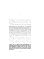
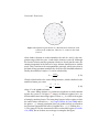
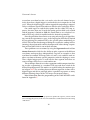
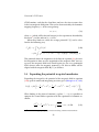
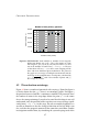
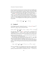
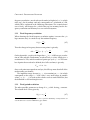
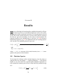
Figure 1.1 shows the energy spectrum of a 2D harmonic oscillator. In
figure A the case for no rotation is shown and the energy spectrum of a 2D
harmonic oscillator is shown. In figure B the critical rotation limit Ω ∼ ω⊥
is shown. Close to critical rotation the levels are not degenerate and the
energy between the lz = 0 and lz = k state is k ~(ω⊥ − Ω). The energy
difference between two following lz states with same nL is given by ~(ω⊥ −
Ω).
5
C HAPTER 1: R OTATION
5
4
3
2
1
5
4
3
2
1
-4 -3 -2 -1
0
1
2
3
4
A
-2 -1
lz
B
0
1
2
3
4
lz
Figure 1.1: Figure A shows the situation without any rotation for a 2D
harmonic oscillator (Ω = 0). Figure B shows the case for rotation frequencies close to critical rotation (Ω ∼ ω⊥ ). At critical
rotation Ω = ω⊥ the levels with n = lz have the same energies
and thus are infinite degenerate. These are called the Landau
levels. The level with nL = 0 is called the lowest Landau Level
(LLL).
1.4
Vortices
So far everything was only on the level of single particle physics and the
next step is to look at the wavefunction of a Bose-Einstein condensate (BEC)
set into rotation. In order to do so a comparison between rotation in a classical fluid and in a quantum fluid is made.
1.4.1
Rotation of a classical fluid
The equilibrium velocity field in the lab frame of a rotating classical fluid is
given by
v = Ω × r,
(1.6)
where v is the velocity field at the position r and Ω is the rotation vector.
The curl of the velocity field,
∇ × v = 2 Ω,
is called the “vorticity” of the flow.
6
(1.7)
C HAPTER 1: R OTATION
1.4.2
Rotation of a quantum fluid
The many-body wavefunction of a Bose-Einstein condensate is given by
(Pitaevskii & Stringari, 2003)
p
Ψ(r) = n(r)eiθ(r) ,
(1.8)
where n(r) is the density and θ(r) the phase of the wavefunction at position
r. This phase θ(r) is a global phase which means that all the atoms in the
condensate have the same phase (phase coherence). In a place where the
density is non zero, the velocity field of the condensate is given by (Landau
& Liftshitz, 1977)
v=
~
∇θ(r),
m
(1.9)
where m is the mass of a particle in the condensate and ∇θ(r) is the gradient of the phase. The vorticity of this field is given by
∇ × v = 0,
(1.10)
because the curl of a gradient is zero1 . This seems to imply that it is forbidden for the condensate to have rotation. This problem of having no rotation
was solved by Feynman (Feynman, 1955) who introduced the concept of
singularities in the phase function. The singularities are shown in the density function as zero points (vortices). This solves the problem because with
these singularities in the phase function it is possible to have rotation in the
condensate and still have phase coherence.
1.4.3
Vortex filling factor
To characterise the rotation of a condensate, the circulation around the condensate is used
I
I
~
h
v · dl =
∇θ(r) · dl = Nv ,
(1.11)
m C
m
C
where Nv is the number of singularities (vortices) in the condensate. Following from the classical fluid the value for the coarse grained velocity is
given by
I
ZZ
ZZ
v · dl =
(∇ × v) · dS =
2Ω · dS = 2 ΩA,
(1.12)
C
1
S
S
Care need be taken here, because this is only true for simply connected domains.
7
C HAPTER 1: R OTATION
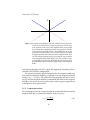
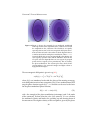
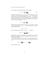
A
Nν
Figure 1.2: Graphical representation of a Bose-Einstein condensate with
vortices in the condensate. There are Nv vortices in the cloud
of area A.
where Stokes’ theorem is used to introduce the curl of v and S is the integration range which has area A and surface element vector dS. Although
the classical velocity and the quantum velocity are clearly not the same, the
contour integration in the limit of a large contour should recover similar
result. This is similar to the correspondence principle, which states that in
the limit of large quantum numbers the classical result should be obtained.
Finally, the number of vortices Nv can be calculated by
2mΩ
A.
(1.13)
h
Closely related to this is the vortex filling fraction ν, which is defined as the
number of atoms per vortex
Nv =
ν=
N
N h
=
,
Nv
A 2mΩ
(1.14)
where N is the number of atoms.
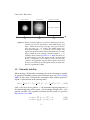
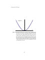
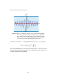
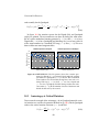
The vortex filling fraction is a parameter to indicate in which rotation
regime the system is. In figure 1.3 images of different regimes for ν are
shown and the most interesting regime is where ν ≤ 10, which is the regime
of strongly correlated states. The interesting features in this regime are that
the vortex lattice will melt at ν ∼ 10 (Cooper, Wilkin, & Gunn, 2001) and at
the point ν ∼ 1 strongly correlated states are produced that are related to
the fractional Quantum Hall effect (Laughlin for ν = 1/2, Pfaffian for ν =
1). The group of Chu has announced to have reached this regime (Gemelke
et al., 2010), but so far there are no images to complete the figure.
8
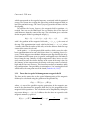
C HAPTER 1: R OTATION
slow rotation
mean-field
strongly correlated
No image available
~105
~103
~10
Figure 1.3: Shown are three regimes for ν the most left image is for slow
rotation (can also be described by mean-field theory) and
large ν which means many atoms per vortex (in the shown
only one vortex on ∼ 105 atoms). The middle image is in
the mean field regime ν ∼ 103 and has a lot of vortices. This
regime can still be described with mean field theory. The right
image should show the strongly correlated regime ν ≤ 10,
which has been reached (Gemelke et al., 2010), but there are
no similar images so far. This regime would - in mean field
theory - correspond to a few atoms per vortex, but the term
vortices is not applicable, because in this regime, mean field
theory is not valid anymore.The figures shown are taken from
previous experiments at ENS.
1.5
Potential stability
When rotating a 2D harmonic anisotropy, due to the anisotropy a window
of dynamical instability around critical rotation opens up (Guery-Odelin,
2000). To show that, a 2D harmonic anisotropic single particle potential Dipod - is placed inside of the rotating frame,
1
1
2
2
U (r) = mω⊥
x2 + y 2 + mω⊥
x2 − y 2 − mΩ2 x2 + y 2 ,
2
2
2
(1.15)
with m the mass of the particle, ω⊥ the harmonic trapping frequency, Ω
the rotation frequency of the system, the anisotropy strength and x, y the
position variables. The equations of motion for this system are given by
(Rosenbusch et al., 2002)
2
ẍ − 2Ω ẏ + ω⊥
(1 + ) − Ω2 x = 0
(1.16)
2
ÿ + 2Ω ẋ + ω⊥
(1 − ) − Ω2 x = 0.
(1.17)
9
C HAPTER 1: R OTATION
From these equations one
that the
can
potential is dynamically un√ deduce√
stable in the range Ω ∈ ω⊥ 1 − , ω⊥ 1 + . Dynamical instability means
that the potential becomes anti-trapping in one or more directions. In the
case of the Dipod there are two directions that are opening up depending
on which side of the critical rotation the Dipod is rotating. This makes the
anisotropic harmonic potential an unsuitable candidate for rotating close to
critical rotation. With a higher-order potential it should be possible to keep
the atoms stabilised up to critical rotation.
A first try to solve this problem was done by taking a potential of the
next higher order - Tripod (Rath, 2010), where the potential is given by
η
1
2
U (r) = mω⊥
1 − α 2 x2 + y 2 −
3x2 y − y 3 .
2
3
(1.18)
Here the notation of (Rath, 2010) is used: α = Ω/ω⊥ and η = 27/8. The
potential has a region of stability within the dynamical unstable regime.
This region has the shape of a triangle and can be characterised by three
end points
1 − α2
ŷ
η
√ 1 − α2
1 − α2
r3 = 3
x̂ −
ŷ
2η
2η
√ 1 − α2
1 − α2
r4 = − 3
x̂ −
ŷ.
2η
2η
r2 =
(1.19)
(1.20)
(1.21)
These points are equally spaced on a circle with radius
R=
1 − α2
.
η
(1.22)
This shows that in the limit of critical rotation α → 1, the stable region
vanishes and thus the potential is destabilised.
A solution for rotating at critical rotation exists in the form of a Quadpod which can be produced with phase modulation (see Chapters 6 for the
shaping and 10 for rotating the shaped potential).
10
C HAPTER 2
Setup
HE experimental setup is in some detail discussed by Steffen Patrick
Rath (Rath, 2010) in his thesis and to full extend in the PhD thesis of
Marc Cheneau (Cheneau, 2009). The description given in this chapter
is in principle a summary of both with some extra care on detail when
describing the TOP trap, which is used to shape and rotate the potential.
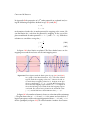
The setup is mainly divided into two chambers: the first chamber “MOT
chamber” to trap and pre cool atoms from a background gas and the second
chamber “Science cell” which is used to further cool, obtain a condensate
(or cold thermal cloud) and finally manipulate the cold atom cloud. In figure 2.1 these chambers are marked and it is shown that they are spatially
separated and connected by a magnetic transport1 .
T
2.1
Sequence
Initially, 87 Rb atoms are captured from a background vapour in a MagnetoOptical Trap (MOT) (Raab, Prentiss, Cable, Chu, & Pritchard, 1987)2 . Then
the cloud is compressed by detuning the MOT laser beams (cMOT) (Townsend
et al., 1995) and prepared for transporting by loading into a quadrupole
trap. Next the cloud is magnetically transported (Greiner et al., 2001)3 and
loaded into a quadrupole trap in the ‘Science cell’. In the quadrupole trap
the evaporative cooling (Ketterle & Druten, 1996) is started and before the
losses due to Majorana spinflips (Brink & Sukumar, 2006) become too large
1
The magnetic transport is based on the Munich model (Greiner, Bloch, Hänsch, &
Esslinger, 2001)
2
This initial trapping stage lasts for ∼ 15 s and captures ∼ 6 · 109 atoms
3
The transport is done over 0.5 m and takes ∼ 5 s during which ∼ 2.6 · 109 atoms are
conserved.
11
C HAPTER 2: S ETUP
Magnetic Transport
TOP coils
MOT chamber
Quadrupole coils
Science cell
Figure 2.1: The 87 Rb setup used to do the experiments. The experiment
is divided into two main chambers: The “MOT chamber”,
where the atoms are captured and pre-cooled from a background gas, and a “Science cell”, where further cooling is
done as well as the manipulation of the cloud. The two chambers are connected by a magnetic transport based on the Munich model (Greiner et al., 2001).
the cloud is transferred into a Time-averaged Orbiting Potential (TOP) trap
(Anderson et al., 1995; Petrich, Anderson, Ensher, & Cornell, 1995), where
the evaporative cooling (Rath, 2010) is continued until a Bose-Einstein condensate (BEC) is reached (Anderson et al., 1995; Davis et al., 1995)4 . While
the cloud is in the TOP trap, the gradient of the quadrupole field is lowered
in order to decrease the mechanical stress on the coil holders, when rapidly
turning off the magnetic trap. After the sequence, absorption imaging is
used to characterise the cloud.
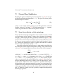
2.2
Time-averaged Orbiting Potential (TOP) trap
An extensive study of the TOP trap is given in Part I, but here we will list
some experimental properties of the TOP trap used in our setup.
The TOP trap is based on a quadrupole trap with additionally a rotating homogeneous bias field, which lets the zero magnetic field point rotate
4
The Bose-Einstein condensate contains ∼ 105 atoms and is reached after ∼ 50 s of
evaporative cooling in the TOP trap.
12
C HAPTER 2: S ETUP
around the cloud. The rotation frequency of our TOP bias field is on the order of ωT = 2π × 10 kHz, but since the domain of interest here is bounded
- for large ωT by the bandwidth of the amplifiers and for low ωT by the micromotion in the trap - there is some interest in finding the right frequency5 .
The currents in the TOP coils are produced using two stereo audio amplifiers (Crest CPX 2600), one for each pair. The amplifiers have a bandwidth
of 5Hz − 50 kHz.
2.2.1
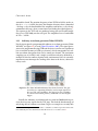
Arbitrary waveform generator (Tabor WW1072)
For the input signals a programmable arbitrary waveform generator (Tabor
WW1072, see figure 2.2) is used (Tabor Electronics, 2005). The signal generator can be programmed using GPIB and the device used in our experiment
has an internal memory of 2 Mb per channel, which corresponds to 2 million waveform data points that can be stored per channel. The maximum
sampling rate is 100 MS/s and a single waveform needs to be defined by a
multiple of 4 in the number of points with a minimum of 64. It is extremely
important to not interrupt the sending of the data to the device, otherwise
it may crash.
Figure 2.2: The Tabor WW1072 Arbitrary Waveform Generator. The generator has two outputting channels, used as input signals for
the two TOP coils amplifiers. The device has the possibility
to send waveform data points by GPIB and wait for a digital
trigger.
Initially the Arbitrary waveform mode was used in Gated mode to generate the necessary signals for the TOP trap. This had the disadvantage of
only being able to send one waveform. To give an example we are only able
5
We have investigated 2π × 5 kHz and 2π × 20 kHz to see if the evaporation can be done
more efficiently. For more information about the choice of ωT we refer to Part I.
13
C HAPTER 2: S ETUP
to send one waveform lets take a sine and a cosine for each channel respectively, then when a digital trigger is send to the device it output the sine and
cosine. When the digital trigger is taken stopped the outputting is stopped.
To have a different signal afterwards new data has to be send to the device.
One could argue to send the data points for the whole TOP trap sequence, but since there are 32 to 64 data points per bias field cycle needed
and the memory is limited to 2MB, this would limit us to a couple of seconds of TOP trap, which is insufficient for the desired experiments.
Since the procedure above limits us to using only one type of signal during a run of the experiment we were, in the largest part of this thesis, limited
by just replacing the standard TOP by the specific (phase modulated) potential. This had the disadvantage of doing the evaporative cooling in these
(rotating) shaped potentials and the decompression either during evaporation or afterwards which is not an ideal situation.
These problems were overcome by using the Segmented mode in Continuous Run mode which has the ability to make segments with different
waveforms and repeat these independently. To given an example we first
send data for a normal TOP trap with a sine and a cosine and then send another waveform with more specific properties to do the shaping we want.
Then a digital trigger pulse is used start the first segment and when we
want to change to the next we send another one.
This technique allowed use to do evaporation and decompression (during or after evaporation) in a standard TOP trap and then switch to the
desired shaped potential. This mode was used for taking the rotation spectra in figure 10.1. The switching between different segments is done with a
digital trigger and this in principle makes it possible to generate as many
different (rotating) shapes of the TOP trap as the memory allows6 .
More information about the programming of the Tabor WW1072 can be
found in Appendix C.
6
While this thesis was written, the group tried to optimise the sequence, as there seemed
to be some triggering issues; for this reason no further data could be taken before the writing
of this thesis
14
Part I
Standard TOP trap
15
C HAPTER 3
TOP trap
- A quadrupole trap is the simplest purely magnetic trap, but it has the disadvantage of a vanishing magnetic field
at the centre. This zero point causes non-adiabatic Majorana spin
flips (Brink & Sukumar, 2006) and thus atom losses. To overcome this problem Petrich et al. introduced the TOP (Time-averaged Orbiting Potential)
trap (Petrich et al., 1995). It is created by adding a rapidly rotating homogeneous bias field, which is rotating around the axis defined by the centres of the quadrupole field coils (Minogin, Richmond, & Opat, 1998). This
field places the zero magnetic field point on a circle outside of the cloud
rather than having it in the centre. At the same time a confining harmonic
averaged potential is experienced by the atoms, which is required for keeping them trapped. The use of this trap allowed the Cornell-group to create
the first Bose-Einstein condensate (BEC) in a dilute atomic gas of rubidium
atoms (Anderson et al., 1995). Afterwards, BECs were also created using a
plug beam to ‘plug’ the centre (Davis et al., 1995), a static non-zero minimum magnetic Ioffe-Pritchard (IP) trap (Mewes et al., 1996), and finally in
2001 also with a purely optical crossed dipole trap (Barrett, Sauer, & Chapman, 2001). The choice of our group was to use the TOP trap because it
provides good optical access and great flexibility. Moreover, we can use
the rotating bias field and tune its parameters for shaping and rotating the
potential.
Q
UADRUPOLE TRAP
3.1
Magnetic trapping
As mentioned above, the simplest purely magnetic trap is a quadrupole
trap. The setup of this consists of two coils placed at exactly twice their
radius d from one another with their centres aligned on the z-axis. The cur17
C HAPTER 3: TOP TRAP
U
r
Figure 3.1: Potential of a quadrupole trap. The solid line shows the potential for atoms which have a negative projection of their magnetic moment on the axis of the magnetic field. At the centre
the potential has a minimum and the atoms prefer to seek the
lowest energy (low-field seekers). The dashed line shows the
potential for atoms which have a positive projection of their
magnetic moment in the direction of the magnetic field. They
can lower their potential energy by leaving the trap, and thus
are untrappable (high-field seekers). It is not possible to have
a maximum in the magnetic field (Earnshaw’s theorem), thus
the high-field seekers can not be trapped with static magnetic
fields.
rent flowing through each coil is equal, but oppositely circulating. This is
called the anti-Helmholtz configuration.
The trap is based on the physical property that the magnetic moment µ
of an atom in a magnetic field B(r) at position r has the magnetic potential
energy U (r) = −µ · B(r). This potential energy provides not only a Larmor
precession of the magnetic moment µ around the direction of the magnetic
field B(r), but also a force that attracts atoms with a negative projection to
a minimum in the magnetic field.
3.1.1
Larmor precession
The Larmor precession of a magnetic moment µ around the direction of the
magnetic field B(r) is characterised by the Larmor frequency
µ · B(r) ,
ωL = (3.1)
~
18
C HAPTER 3: TOP TRAP
which corresponds to the angular frequency associated with the potential
energy. The system tries to align this precessing with the magnetic field, to
lower the potential energy. The Larmor frequency provides the time scale for
the aligning.
To calculate the Larmor frequency, the magnetic field at position r is
needed. One can use the Biot-Savart law to calculate this in the limit of
small distances from the centre of the trap. The calculation gives a relation
for the magnetic field of a quadrupole trap b(r),
b(r) = b(x − xi ) x̂ + b(y − yi ) ŷ − 2b(z − zi ) ẑ,
(3.2)
with b the gradient of the magnetic field and ri = (xi , yi , zi ) the centre of
the trap. This approximation is only valid in the limit |r − ri | d, where
d stands, either for the radius of the coils, or for the distance from the trap
centre to the centre of each coil.
At the point r = ri the magnetic field vanishes, which causes the adiabatic approximation to be non-valid. Since there is a vanishing Larmor frequency, which triggers non-adiabatic Majorana spin flips that flip the magnetic moment of the atoms to an, in general, untrappable state and induces
losses from the trap. Initially at high temperatures these losses are relatively small, because the relative density in the centre of the trap is low. On
the contrary, at low temperatures the density at the trap centre is relatively
high and the loss rate increases. This forced researchers to introduce other
trap configurations. One possibility is to introduce a ‘fast’ rotating bias field
which moves the zero point out of the cloud (Petrich et al., 1995).
3.1.2
Force due to spatial inhomogeneous magnetic field
The force on the atoms due to the spatial inhomogeneity of the magnetic
field may be calculated using the gradient of the potential by
F (r) = −∇U (r) = −µ∇b(r),
where µ is one of the possible negative projections of the magnetic moment in the direction of the magnetic field and b(r) the magnitude of the
magnetic field at position r. The calculation can be simplified by taking the
trap centre being ri = (0, 0, 0). It follows that the force on a particle with
magnetic moment µ equals to
F (r) = −µ b ∇
p
r̄
x2 + y 2 + 4z 2 = −µ b p
,
2
x + y 2 + 4z 2
19
(3.3)
C HAPTER 3: TOP TRAP
where r̄ = x x̂ + y ŷ + 4z ẑ is similar to position vector r but with a rescaled
z-axis. In the xy-plane the force turns out to be constant and pointing towards the centre, except for the point r̄ = 0, which is a singular point.
3.2
Rotating bias field
To remove the zero magnetic field point from the centre of the cloud a rotating bias field is added in the xy-plane (Minogin et al., 1998). This rotating
bias field is given by
h
i
B(t) = −B0 cos(Φ(t)) x̂ + sin(Φ(t)) ŷ ,
(3.4)
with B0 the magnitude of the rotating bias field and Φ(t) is the phase function, which for a standard TOP trap is given by Φ(t) = ωT t where ωT is the
angular frequency.
A rotating homogeneous bias field displaces the zero magnetic field
point out of the cloud and lets it rotate at a radius r0 which is called the
“radius of death”. Figure 3.2 shows the displacement of a quadrupole magnetic field projection due to a bias field in the co-rotating frame. From the
figure it can be seen that the zero magnetic field point is actually shifted in
the direction opposite to the direction of the bias field. Using this makes it
possible to define the “radius of death” r0 1 :
B0
.
(3.5)
b
The total magnetic field is simply recovered by adding the bias field to
the quadrupole field (for simplicity we take the centre of the initial static
trap to be at the centre of the coordinate system ri = 0),
h
i
B T (r̃, Φ(t̃)) = B0 x̃ − cos(Φ(t̃)) x̂ + ỹ − sin(Φ(t̃)) ŷ − 2z̃ ẑ , (3.6)
r0 =
where we have introduced the phase function Φ(t̃) = 2π t̃, which is used to
define the phase of the rotating bias field during one cycle. The dimensionless variables r̃ = r/r0 is the position vector defined in units of the “radius
of death”, and t̃ = ωT t/2π a time variable normalised to one rotation cycle.
The magnitude of the total magnetic field BT (r̃, Φ(t̃)) is given by
q
BT (r̃, Φ(t̃)) = B0 1 + x̃2 + ỹ 2 + 4z̃ 2 − 2 x̃ cos(Φ(t̃)) + ỹ sin(Φ(t̃)) . (3.7)
1
The experiment described in this thesis has a “radius of death” that is on the order of
' 1 mm
20
C HAPTER 3: TOP TRAP
B
B0
r
r0
Figure 3.2: The magnetic field of the quadrupole field in the rotating
frame of the bias field. The magnetic field is shifted by the bias
field. The dashed blue line is the original quadrupole field
without bias field and the thick solid line is the quadrupole
field with the bias field. B0 is the magnitude of the spatial homogeneous bias field and r0 is the displacement of the zero
magnetic field point (the “radius of death”).
3.3
Time-averaged potential
Since the potential is rapidly rotating in time, some important limits to the
rotation frequency of the bias field are apparent. The first requirement is
that at all times the magnetic moments of the atoms need to be able to follow the rotation of the magnetic field. This limit can be characterised by the
Larmor frequency (a theoretical investigation of the adiabatic approximation
is done by (Franzosi, Zambon, & Arimondo, 2004)), associated to the rotating bias field:
µ · B(r, t)
;
~
ωT ωL .
ωL = −
(3.8)
Equation (3.8) gives the requirement for the adiabatic approximation to be
valid and gives an upper limit to the rotation frequency (in our experiment2
the Larmor frequency is of order 2π × 5 MHz).
On the other end, there is a lower limit which states that the movement
of the zero magnetic field point is much faster then the Centre-Of-Mass
2
The experiments are done with 87 Rb in the states |F = 1, mF = −1i and |F = 2, mF =
+1, +2i (Rath, 2010) with Landé factors g1 = 1/2 and g2 = −1/2
21
C HAPTER 3: TOP TRAP
(COM) motion, such that the cloud does not have the time to come close
to the zero magnetic field point. This can be characterised by the harmonic
trapping frequency ω⊥ of the averaged trap:
ωT ω⊥ ,
(3.9)
where ω⊥ (which will be derived later on), in the experiments described by
this thesis3 , is of the order of 2π × 10 Hz.
When these limits are valid, the average potential U (r̃) can be calculated in the following way:
1
Z
BT (r̃, t̃) dt̃
(3.10)
Z 1q
= µB0
1 + x̃2 + ỹ 2 + 4z̃ 2 − 2 x̃ cos(Φ(t̃)) + ỹ sin(Φ(t̃)) dt̃.
UT (r̃) = µ
0
0
This potential shows the importance of the limit in equation (3.8), because
the integration is done over the magnitude of the magnetic field. An average over the magnetic field itself would again give rise to a quadrupole
field, whereas now the magnetic moments µ are able to follow and be
aligned with the magnetic field B(r̃, t̃) at all times.
3.4
Expanding the potential in spatial coordinates
Expanding the integral in the potential of the magnetic field in equation
(3.10) up to 4th -order and integrating over time gives (Minogin et al., 1998)
UT (r̃) = µB0
1 2
1 4
2
2 2
4
6 6
1+
r̃ + 8z̃ +
r̃ + 32r̃ z̃ − 128z̃ + O(r̃ , z̃ ) .
4
64
(3.11)
When looking in the plane of rotation (xy-plane z̃ = 0), it is possible to
compare the second order expansion with the equation of a harmonic oscillator,
µ b2
1
2 2
r2 = mω⊥
r ⇒ ω⊥ =
4B0
2
3
s
µ b2
' 2π × 10 Hz.
2mB0
The harmonic trapping frequency is measured using oscillation measurements
22
(3.12)
C HAPTER 3: TOP TRAP
A similar comparison can be done for the 4th -order terms,
1 µ b2 4
r = κr4
64 B0
1 µ b2
κ=
> 0,
64 B0
(3.13)
which implies that when the harmonic term is compensated by the centrifugal potential, the TOP-trap still has a quartic term which is trapping. Comparing this to the Ioffe-Pritchard trap, which has κ < 0, it is seen that in the
TOP a natural trapping mechanism arises, whereas in the case of the IoffePritchard trap an additional anharmonic trap was needed (Bretin, Stock,
Seurin, & Dalibard, 2004). If we compare these results with Appendix A it
corresponds to the case b = 0 and a > 0 and thus trapping.
In figure 3.3 the exact potential of the TOP trap on the x̃ axis is shown.
It is important to note, that at the centre a clear harmonic behaviour is visible at distances smaller then the “radius of death”, whereas outside of the
“radius of death”, the trap becomes linear again, which is to be expected
since the quadrupole trap is linear and the rotation outside the “radius of
death” is just an addition of linear fields with the same slope, which is a
linear potential itself.
3.5
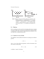
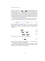
Experiments using TOP trap to shape potentials
The Oxford-group have been using the TOP trap as basis for their research
on rotating systems, but they modulated the trajectory of the zero magnetic
field point to shape the averaged potential (Arlt et al., 1999). In contrast to
the phase modulation used in our group. More about shaping (Part II) and
rotation (Part III) in the rest of this thesis.
23
C HAPTER 3: TOP TRAP
UΜB0-1
2.0
1.5
1.0
0.5
xŽ
-3
-2
1
-1
2
3
Figure 3.3: The thick blue line is the exact time averaged potential of the
TOP trap. The vertical axis is in units of µB0 and the horizontal axis shows for reasons of simplicity the radial x-axis of the
trap in units of the “radius of death”. The centre clearly shows
at lowest order a harmonic trap, whereas outside of the “radius of death” there is no influence from the rotation and the
trap again behaves like a standard quadrupole trap. The thin
line is the potential approximated up to 2nd -order. Within the
“radius of death” the two have good overlapping, but outside
a clear difference is shown.
24
C HAPTER 4
Discretisation
field - The TOP trap uses a rapidly rotating bias field to
make the zero magnetic field point cycle around the cloud (Minogin
et al., 1998). In order to be able to rotate the cloud, it is necessary to
introduce an anisotropy, which at a later stage can be rotated. The strongest
nth -order anisotropy can be created with just using n zero magnetic field
points, which are distributed evenly over the cycle in space and time. For
the TOP trap this would mean it starts in one point, stays there a certain
period of time and then “jumps”1 to the next point.
R
OTATING
4.1
Zero magnetic field points
The formalism used in Chapter 3 is based on continuous variables. This
means that the time resolution in principle is infinite, for practical reasons
this is not feasible. The device2 used to generate the signals that are sent to
the amplifiers only accepts lists of data points. This required us to introduce
a formalism for discrete rotation. The position of the zero magnetic field
point can be described by the fast rotating spatial homogeneous bias field
B(Φ(t̃)) (derived from equation 3.4) and the quadrupole field b(r),
r0 (Φ(t̃)) = −
h
i
B(Φ(t̃))
= r0 cos Φ(t̃) x̂ + sin Φ(t̃) ŷ .
b
1
(4.1)
Ideally this happens at infinite speeds, but in practice we are limited by the bandwidth
of the signal amplifiers.
2
The device we use for outputting the signals is an arbitrary waveform generator: Tabor
WW1072.
25
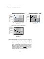
C HAPTER 4: D ISCRETISATION
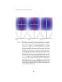
A. N = 2
B. N = 4
C. N = 8
D. N = 16
E. N = 32
F. N = 64
Figure 4.1: Potentials created by having η zero magnetic field points.
From left to right and top to bottom the number of points
per cycle is doubled in each following figure, starting with
2. A. clearly shows the strong Dipod potential; in B. a strong
Quadpod potential is shown; in C. the 8th order is still visible but already the harmonic term is taking over. Figures D
through F are clearly approximating the round TOP trap. The
red circle is at the “radius of death” and the black dots on the
circle are the zero magnetic field points used to calculate the
potential.
The first step is to discretise the phase function such that it only accepts
integer numbers:
i
Φ(t̃) = 2π t̃ → Φ(i) = 2π ,
η
(4.2)
where η ∈ N is the number of zero points during one cycle and i ∈ {0, . . . , η−
1} is the discretised time iterator. However, there is a continuous current
sent through the coils, thus finally, the potential produced is again continuous.
26
C HAPTER 4: D ISCRETISATION
Number of zero points η spectrum
Atom number (a.u.)
50,000
40,000
30,000
20,000
10,000
0
1
10
100
1000
Number of zero points η
Figure 4.2: PRELIMINARY: Atom number vs. number of zero magnetic
field points during one cycle η. The η data points are, from
left to right: 2, 4, 8, 16, 32, 64, 128, 256, 512. There is a clear
rise in the number of atoms from η = 16 to η = 32. The rest
of this thesis will use η = 64 to have atoms. Shaping will be
done with more dedicated phase modulation. The points in
the graph are an average of multiple measurements and the
error bars
errors of each points, calculated by
p are the standard
2
2
σse = hy − hyii /N , with N the number of points and hyi
the average of y-values.
4.2
Discretisation anisotropy
Figure 4.1 shows a number of potentials with varying η. From this figure it
is clearly shown that for η ≤ 8, there is an anisotropy visible. For higher η
the potential starts to look like a continuous standard TOP potential. Since
the number of atoms in the trap drops below the point η = 32 the atoms
do see the strong anisotropy. It needs to be noted that this drop is not well
understood, since the potential of the trap does not seem to change significantly from η = 16 → 32. At this stage, the only reasonable hypothesis we
are able to formulate is that the change of direction of the bias field is too
fast, such that the magnetic moment of the atoms does not follow. Further
investigation could be done, by simulating the system keeping track of the
27
C HAPTER 4: D ISCRETISATION
internal degrees of freedom (omitting the adiabatic approximation).
28
Conclusion and Summary
OP TRAP - The TOP trap is produced by a quadrupole trap in addition to a rapidly rotating bias field. This causes the zero magnetic
field point of the quadrupole to circle around the trap instead of staying fixed in the centre of the cloud.
This trap is an interesting tool for studying rotation, because it has a 4th order potential that is trapping. This means that when an atom cloud is set
into rotation, near the point where the centrifugal force fully compensates
for the harmonic trapping, the system will still be able to keep the cloud
confined in the centre.
The ‘static’ TOP trap, however, does not have the ability to set the cloud
into rotation. This requires us to introduce an anisotropy. Since discretisation of the TOP currents was needed for our equipment, the simplest way
of creating the desired symmetry is by setting the number of zero points
during one cycle equal to the desired anisotropy symmetry. We have done
measurements on these types of anisotropic potentials and it turned out
that there is a minimal number of points needed to be defined to have
atoms in the trap.
It need be noted though that these experiments were done having an
anisotropic TOP trap using the first mode described in section 2.2.1. This
may cause effects that we are not able to explain and needs further investigation.
T
29
C HAPTER 4: D ISCRETISATION
30
Part II
Static Anisotropic TOP trap
31
C HAPTER 5
Phase Modulation
TOP traps do not have the ability to rotate a cloud, because
they are shaped such that the zero magnetic field point has a round
trajectory. Following symmetry arguments, the TOP trap potential is
considered round when the trajectory is round1 and the rotation speed of
the zero magnetic field point is constant. There is a tool required for making
the cloud rotate.
The Oxford-group (Arlt et al., 1999; Hodby, Hechenblaikner, Hopkins,
Maragò, & Foot, 2001) chose to modulate the amplitude of the trajectory,
thereby creating versatile elliptical potentials. The disadvantage using this
method is that the “radius of death” depends on its angular position. This
causes an oscillation of the “radius of death” and this may make it possible
for the zero magnetic field point to enter into the cloud and cause losses.
Our approach is to use phase modulation which holds the “radius of death”
constant over one cycle.
Phase modulation is a method that is based on changing the rotation velocity of the zero magnetic field point. Since only the velocity is modulated,
there is no change of the “radius of death”. Phase modulation provides us
with the tool for shaping and rotating the desired potential.
S
5.1
TANDARD
Formalism
In Chapters 3 and 4 the formalism based on (Minogin et al., 1998) is introduced. This is the basis of our concept of phase modulation of the TOP trap.
1
There is always a ‘static’ anisotropy due to the not perfectly round trajectory of the zero
magnetic field point.
33
C HAPTER 5: P HASE M ODULATION
A
B
Figure 5.1: Figure A shows the potential for an amplitude modulated
TOP trap which has the amplitude in the x-direction to be half
the amplitude in the y-direction. The black dots are equally
spaced points in time of the zero magnetic field point movement and the red circle is the radius of death. Figure B shows
a similar situation but with phase modulation, where = 0.5.
Again the black dots are zero magnetic field points during one
cycle equally spaced in time and the difference between the
two plots is that in figure B there are two regions of grouped
points and two regions of low point density. This is cased by
the phase modulation. The contour plots have dark colours
corresponding to low potential energies and light colours to
high potential energies.
The zero magnetic field point is given in eq. (4.1),
h
i
r0 (Φ(t̃)) = r0 cos Φ(t̃) x̂ + sin Φ(t̃) ŷ ,
where Φ(t̃) was introduced to describe the phase of the rotating zero magnetic field point in units of one zero point cycle t̃. For a standard round TOP
trap the phase function equals Φ(t̃) = 2π t̃ and this can be used as the basis
for the phase modulated phase function,
Φ(t̃) = 2π t̃ + sin(2πN t̃),
(5.1)
with the strength of the phase modulation (anisotropy) and N the order
of the symmetry. To show what the order of the symmetry N is we calculate
the rotational velocity and look at the speeding up and slowing down of
the movement. The angular velocity of the zero point is given by the phase
34
C HAPTER 5: P HASE M ODULATION
velocity
dΦ(t̃)
= 2π + 2πN cos(2πN t̃).
dt̃
(5.2)
The phase modulation changes the speed of the zero magnetic field point
and creates N points where the zero point is maximally slowed down (the
potential in this direction is relatively lower) and N points where the zero
point is maximally accelerated (the potential in this direction is relatively
higher). The velocity depends on the anisotropy strength and an interesting
feature of the phase velocity is that for an anisotropy with > 1/N , there
are phases during a single cycle where the rotation of the zero point actually
changes its direction.
5.2
Time-averaged potential
The rotation frequency is limited by the Larmor frequency (see eq. (3.8)), because it determines the validity of the adiabatic approximation. This means
that the magnetic moments of the atoms need to be able to follow the magnetic field:
ωT (t) ωL ,
where we intentionally wrote ωT (t) to emphasise the fact that the rotation
frequency of the zero magnetic field depends on the phase modulation,
ωT (t) = ωT,i + ωT,i N cos(ωT N t),
(5.3)
with ωT,i the initial rotation frequency of a standard TOP trap. This velocity
is oscillating and the maximum value of this oscillation is given by
ωTmax = ωT,i (1 + N ) .
The new adiabatic approximation validity limit is given by
ωT,i (1 + N ) ωL .
(5.4)
When this limit is fulfilled, it is possible to write the time-averaged potential of a phase modulated TOP trap (eq. (3.10)) as
Z 1q
UT (r̃) = µB0
1 + x̃2 + ỹ 2 + 4z̃ 2 − 2 x̃ cos(Φ(t̃)) + ỹ sin(Φ(t̃)) dt̃,
0
where we now use the phase function Φ(t̃) from eq. (5.1).
35
C HAPTER 5: P HASE M ODULATION
5.3
Expanding the phase modulated potential
Solving the integral relation of the phase modulated potential is extremely
difficult if not impossible to do, so first the potential was expanded in spatial coordinates and then integrate over one cycle. The expanded dimen(n)
(n)
sionless potential (ŨT (r̃) = UT (r̃)/µB0 where n stands for the nth -order
expansion) is given by
(0)
(5.5)
ŨT (r̃) = 1
(1)
ŨT (r̃) = x̃ J1 ()δN,1
1h 2
(2)
ŨT (r̃) =
x̃ + ỹ 2 1 + J2 (2)δN,1
4
i
+ x̃2 − ỹ 2 J1 (2)δN,2 + 8z̃ 2
1h 3
(3)
ŨT (r̃) =
−x̃ J1 ()δN,1
8
−x̃ỹ 2 J1 ()δN,1
− 16x̃z̃ 2 J1 ()δN,1
i
+ (x̃3 − 3x̃ỹ 2 ) (J3 (3)δN,1 + J1 (3)δN,3 )
1h 4
(4)
x̃ + ỹ 4 (1 − 5 (J4 (4)δN,1 + J2 (2)δN,2 − J1 (4)δN,4 ))
ŨT (r̃) =
64
+ 4 x̃4 − ỹ 4 (J2 (2)δN,1 − J1 (2)δN,2 )
+ x̃2 ỹ 2 (2 + 30 (J4 (4)δN,1 + J2 (4)δN,2 − J1 (4)δN,4 ))
i
+ z̃ 2 32(x̃2 + ỹ 2 ) + 96(x̃2 − ỹ 2 ) (J2 (2)δN,1 − J1 (2)δN,2 ) − 128z̃ 4 ,
where δN,p with p ∈ N is the Kronecker delta used to indicate that it belongs
to the pth order of symmetry. Jn (x) is the nth -order Bessel function for x.
These results are original in the sense that, this has not been done before
and it can be applied more generally than the result from previous studies
(Minogin et al., 1998). The result from these studies can even be retrieved
by taking a special case (N = 0 and/or = 0).
The standard TOP trap has the properties = 0 and/or N = 0. Checking the potential using these parameters, we get
1 2
1 4
2
2 2
4
UT (r̃) = µB0 1 +
r̃ + 8z̃ +
r̃ + 32r̃ z̃ − 128z̃
,
4
64
giving the same result for the standard TOP trap as eq. (5.5).
36
C HAPTER 5: P HASE M ODULATION
The case N = 1, in principle, off centres the cloud with respect to the
“circle of death”. This case might be interesting for studying clouds that are
rapidly rotating around a circle. However, we have not done any further
research on this topic.
The cases N = 2, 3, 4 will play a vital role in the coming parts of this
thesis, because with these potentials we were able to create cloud that are
rapidly rotating around their centre-of-mass. With the theoretical results
obtained in this section we were able to explain some interesting phenomena appearing in our experiments.
37
C HAPTER 5: P HASE M ODULATION
38
C HAPTER 6
Potential Shaping
HAPING - The first efforts of shaping a TOP trap have been done by the
Oxford-group (Arlt et al., 1999). They used amplitude modulation to
produce an elliptical path for the zero magnetic field point. This again
produces an elliptical time-averaged potential. This causes the “radius of
death” to vary in time and possibly cut into the cloud. Our approach is to
phase modulate the rotational movement. This allows use to make similar
elliptical potentials using N = 2 - a (Dipod) - introduced in eq. (5.1), without changing the “radius of death”. On the other hand, it gives us also a
framework for producing higher order potentials.
S
6.1
Dipod
The Dipod potential is obtained by taking the order of symmetry parameter
N = 2, thus retreiving
Φ(t̃) = 2π t̃ + sin(4π t̃);
the averaged potential up to 2nd -order in the xy-plane corresponding to
that is given by
1 2
UT (r̃) = µB0 1 +
x̃ (1 + J1 (2)) + ỹ 2 (1 − J1 (2)) .
4
(6.1)
To simplify the equation, one has to note that the Bessel function J1 (2) has
only a limited range of values, which allows us to define a new variable
j ∈ [J1min , J1max ] and replace the Bessel function J1 (2) by j, thus it follows
39
C HAPTER 6: P OTENTIAL S HAPING
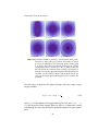
N=2
N=3
N=4
Figure 6.1: The order of symmetry N for the potential in the xy-plane.
The red circle in the upper row of figures is the circle of death.
From left to right are, respectively, shown the potentials for
N = 2, N = 3 and N = 4 with an anisotropy = 0.5. The
figures in the upper row are contour plots of the potentials,
where dark purple corresponds to lower energies and light
purple to higher energies. The plotted lines show the axes of
the figures in the lower row, where the colours of the lines
in the upper plot correspond to the line colours in the lower
plots. The potential for N = 2 has a Dipod shape and as can
be seen from the cuts, the horizontal and vertical axes have
different harmonic shapes (trapping frequencies). The case
N = 3 - a Tripod - has a three fold symmetry and the horizontal cut shows the asymmetry, whereas the vertical one is
symmetric. The case N = 4 - a Quadpod - shows the four
fold symmetry and the vertical and diagonal cuts show the
two main axes of the Quadpod. From these cuts it can be seen
that the diagonal directions are less tightly confining than the
vertical/horizontal direction.
40
C HAPTER 6: P OTENTIAL S HAPING
for the potential that
UT (r̃) = µB0
1 2
2
1+
x̃ (1 + j) + ỹ (1 − j) .
4
In figure 6.2, the Bessel function J1 (k) is given with the possible values
of j given by the light blue area. The Dipod potential corresponds to the
case k = 2.
The left hand graphics in Figure 6.1 show - in the upper row - a contour
plot of the averaged potential, and - in the lower row - the cuts on the xaxis (blue line) and y-axis (red line). It is evident that the two cuts in the left
column have different trapping frequencies. These trapping frequencies are
given by
p
ωx = ω⊥ 1 + j;
(6.2)
p
ωy = ω⊥ 1 − j,
(6.3)
where ωx (ωy ) is the trapping frequency in the x-direction (y-direction) and
ω⊥ the trapping frequency in the xy-plane for the standard TOP trap.
Using these relations, we can define the anisotropy in terms of the trapping frequencies ωx and ωy :
j=
ωx2 − ωy2
.
ωx2 + ωy2
(6.4)
Since the Bessel function J1 (2) up to 1st -order, in , is given by j ' ,
these results correspond to the used by the Oxford-group (Arlt et al., 1999;
Hodby et al., 2001). The range of anisotropies is obtained by taking the
minimum and maximum of Bessel function J1 (2),
j ∈ J1min (2), J1max (2) = [−0.58, 0.58] .
(6.5)
6.2
Tripod
The Tripod potential is obtained by using N = 3 in eq. (5.5), up to 3rd -order
in the xy-plane, thus the potential becomes
1 2 1 3
2
UT (r̃) = µB0 1 + r̃ +
x̃ − 3x̃ỹ J1 (3) .
4
8
The potential in the xy-plane is shown in the upper middle graph in figure
6.1. There a clear three fold symmetry is visible. The red and blue lines
41
C HAPTER 6: P OTENTIAL S HAPING
show two directions of interest in the potential. In the lower middle graph,
the line colours correspond to these special direction. The red line shows
that on the y-axis the potential is symmetric, whereas the blue line shows
the asymmetric behaviour in one of the Tripod’s symmetry directions.
In figure 6.2 the general Bessel function J1 (k) is shown, for the 3rd order k = 3 needs to be used. Also for the Tripod the replacement J1 (3) →
j can be done, but care needs to be taken, because the s corresponding to
a values of j for the Tripod potential is different from the s corresponding
to the same j for the Dipod potential. Following from this replacement, is
the potential
UT (r̃) = µB0
6.3
1 2 1 3
2
1 + r̃ +
x̃ − 3x̃ỹ j .
4
8
Quadpod
The Quadpod potential is obtained by using N = 4 in eq. (5.5), up to 4th order in the xy-plane, thus the potential becomes
1
1
UT (r̃) = µB0 1 + r̃2 +
4
64
4
x̃ + ỹ
4
(1 + 5 J1 (4)) + x̃ ỹ (2 − 30 J1 (4)) .
2 2
The right hand column in figure 6.1 in the first row a contourplot of the
Quadpod potential N = 4 in the xy-plane. Again, the lines drawn in the
contour plot are the directions of interest and symmetry. The red line shows
that the potential in the direction x = y is lower than in the other (blue line),
which creates the rounded square shape.
The anisotropy can be described with only one parameter J1 (4). This
means that it is possible to make groups of with J1 (4) = j ∈ [J1max , J1min ],
which is sufficient to define the anisotropy. Thus the replacement J1 (4) →
j can be made, but again care needs to be taken when the transformation
back to is made. The replacement transforms the potential into the following form:
UT (r̃) = µB0
1
1
1 + r̃2 +
4
64
4
x̃ + ỹ
4
2 2
(1 + 5 j) + x̃ ỹ (2 − 30 j)
.
The most remarkable feature following from this becomes apparent when
j = 0 and = 0 (the standard TOP trap), which has a potential that is
perfectly symmetrical, but this is not only the case for = 0. In fact, it is
42
C HAPTER 6: P OTENTIAL S HAPING
J1(kε)
0.6
j
-40
-20
20
40
kε
-0.6
Figure 6.2: Shown is the Bessel function J1 (k) with being marked the
zero crossing (red dots) and the range of values j (light blue
area). At the zero crossings, there is special behaviour of the
potentials at least up to the Quadpod, because their potentials
UT (r̃) equal that of the standard TOP potential with = 0.
true for all such that j = 0. The potential in the case of j = 0 is given by
1 2
1 4
UT (r̃) = µB0 1 + r̃ + r̃ .
4
64
This is remarkable because, as can be seen from figure 6.2, there are a lot of
zero crossings in the Bessel function J1 (4). From now on we will use the
variable j to define the anisotropy.
43
C HAPTER 6: P OTENTIAL S HAPING
44
C HAPTER 7
Anisotropy Strength
- the strength of the anisotropy is very important to investigate, because we are modulating the speed of the
zero magnetic field point with phase modulation. This speed modulation may have a big influence on the atoms. For doing this we extend
the formalism from Chapter 4 with the phase modulation phase function
from Chapter 5.
A
NISOTROPY STRENGTH
a
b
c
N=2
N=3
N=4
Figure 7.1: Shown are the discrete potentials for N = 2, N = 3 and
N = 4. Each contour plot shows the zero magnetic field points
spread out over the “circle of death” with the time in between
the points being fixed. The number of points η = 64 and the
anisotropy = 0.5, which corresponds to j ' 0.44 for the Dipod, j ' 0.55 for the Tripod and j ' 0.58 for the Quadpod.
45
C HAPTER 7: A NISOTROPY S TRENGTH
7.1
Discrete Phase Modulation
Recalling the phase modulation phase function from eq. (5.1) we can apply the discretisation transformation t̃ → i/η. This gives the discrete phase
modulation phase function
i
i
Φ(t̃) = 2π + sin 2πN
,
(7.1)
η
η
where η is the number of time points per cycle. The potentials are shown
for three values of N in figure 7.1. The black points show η = 64 points,
where the period of time in between two points is constant.
7.2
Atom losses due to a static anisotropy
To see what the anisotropy strength does at the level of the atoms, we look
at what happens to the number of atoms when changing the anisotropy
strength while keeping the other parameters constant. In figure 7.2 the
results of these measurements are plotted and an interesting feature is that
the decrease in atom number in both the Dipod and Quadpod is linear
in , whereas the Tripod seems to have a plateau first and then a sudden
decrease in the atom number around = 0.25.
A possible explanation for the decrease in atom number would be that
the velocity of the zero magnetic field point is too high. This can be checked
with eq. (5.2) and comparing the maximum value of this while changing N :
dΦ(t̃) = 2π + 2πN ,
dt̃ max
which for N = 2 and the point of total loss = 0.3 gives (dΦ(t̃)/dt̃)max =
1.2 π. For N = 3 and = 0.3, it becomes (dΦ(t̃)/dt̃)max = 0.9 π. Finally, for
N = 4 and = 0.5, we find (dΦ(t̃)/dt̃)max = 2 π. These results, in principle, are connected to the results obtained in section 4.2. Since there are
no clear indications for the loss of atoms, except for the change of velocity of the bias field that the atoms experience, it would be interesting to
do simulations on the quantum motion of an atom. These simulations then
would need to keep track of the atoms internal degree of freedom (no adiabatic approximation), and essentially simulate the evolution of two (for
spin 1/2 particles) or three (for spin 1 particles) coupled time-dependent
Schrödinger equations.
46
C HAPTER 7: A NISOTROPY S TRENGTH
40,000
30,000
20,000
10,000
0
Anisotropy spectrum Tripod
Atom number (au)
Atom number (au)
Anisotropy spectrum Dipod
0
0.1
0.2
0.3
0.4
0.5
60,000
45,000
30,000
15,000
0
0
Anisotropy ε
Anisotropy ε
Atom number (au)
Anisotropy spectrum Quadpod
80,000
60,000
40,000
20,000
0
0
0.1
0.3
0.4
0.5
Anisotropy ε
Figure 7.2: PRELIMINARY: Shown is the atom number as a function of
the anisotropy in a static phase modulated TOP trap. Upper left is the Dipod N = 2 potential, upper right the Tripod
potential N = 3 and finally lower left the Quadpod potential N = 4. The Dipod and Quadpod potentials show a linear relation in the decrease of atom numbers, whereas for the
Tripod it looks more like a constant plateau and then a steep
decrease. The points in the graph are an average of multiple
measurements and the error bars
pare the standard errors of
each points, calculated by σse = hy − hyii2 /N 2 , with N the
number of points and hyi the average of y-values.
47
0.1 0.2 0.3 0.4 0.5
C HAPTER 7: A NISOTROPY S TRENGTH
48
Conclusion and Summary
- turned out to be an exhaustive tool for creating
anisotropic traps with any desired symmetry. We have given a strong
formalism, based on the formalism given in Part I, that describes the
potential of the phase modulated TOP trap. This potential is really difficult
to solve analytically, but expanding the magnitude of the magnetic field
in spatial coordinates provided us with the necessary potential in the centre and allowed use to investigate some interesting potential symmetries.
Three different symmetries have been characterised and discussed: the Dipod (N = 2), the Tripod (N = 3) and the Quadpod (N = 4).
Finally, the anisotropy of these potentials has been investigated by looking at the atom number as a function of the strength of the anisotropy. Both
the Dipod and the Quadpod show linear decreasing behaviour until there
are no atoms left. The Tripod on the other hand seems to have an plateau
and then a threshold above which the atom number strongly decreases.
These experiments showed some interesting, but unexplained behaviour
that needs further investigation.
Also it need be noted that these experiments were done in the first run
mode (discussed in subsection 2.2.1), which uses the phase modulated TOP
trap during evaporation and decompressing of the TOP trap.
P
HASE MODULATION
49
C HAPTER 7: A NISOTROPY S TRENGTH
50
Part III
Rotating Anisotropic TOP trap
51
C HAPTER 8
Co-Rotating Frame
- The TOP trap has a natural rotation in the
movement of the zero magnetic field point. The previous chapter
used phase modulation to modulate this rotational movement and
use it to shape the potential. The rotation can only be done in two dimensions and the plane of choice is the xy-plane, which makes the description
of the phase modulation easier but not necessarily less general. The next
step is to set the phase modulated shape into rotation.
The set a system into rotation - in the xy-plane - the rotation matrix
N
ATURAL ROTATION
R(Ωt) =
cos Ωt − sin Ωt
sin Ωt cos Ωt
(8.1)
is used, where Ω is the angular rotation frequency of the rotating system.
8.1
Potential in co-rotating frame
The movement of the zero magnetic field point described by r 0 is set into
rotation by multiplying the equations of motion by the rotation matrix:
r0rot Φ(t̃) = R (Ωt) · r0 Φ(t̃)
= r0 Φ(t̃) + Ωt = r0 Φ(t̃) + 2π δ t̃ ,
where we have introduced δ = Ω/ωT . If we then change the time variable
to a dimensionless time in the rotating frame,
t̃ = (1 + δ)
53
ωT
t
2π
(8.2)
C HAPTER 8: C O -R OTATING F RAME
and take the phase modulation function (eq. (5.1))
Φrot (t̃) = 2π t̃ + sin(2πN t̃) + 2π δ t̃.
(8.3)
This means that when looking in the co-rotating frame the angular frequency of the rotating zero magnetic field point is reduced by a δω⊥ . Important then for the atoms is that in the rotating frame they still see a averaged
potential (eq. (3.9)) with a reduced ωT ,
(1 − δ) ωT ω⊥ .
(8.4)
Since we are interested in the limit of critical rotation which means Ω ' ω⊥ ,
it follows that δ ' ω⊥ /ωT 1, thus validating the limit in eq. (8.4). The
potential in the rotating frame is then given by eq. (3.10) with a redefined
dimensionless time t̃ given by eq. (8.2). Since the integration limits in this
case stay defined over one integration period, the integral keeps having
the same outcome. Only when the limit eq. (8.4) is violated the potential is
not well defined in the co-rotating frame. The potential in the co-rotating
frame is given by the potential in the lab frame (eq. (3.10)) with the phase
modulation function Φ(t̃) given by eq. (5.1):
Z
UT (r̃) = µB0
1q
1 + x̃2 + ỹ 2 + 4z̃ 2 − 2 x̃ cos(Φ(t̃)) + ỹ sin(Φ(t̃)) dt̃.
0
54
C HAPTER 9
Discretising Rotation
- The discretisation needs some special caution, because we need the periods of two rotations to be overlapping. The
first arising for the ‘fast’ rotating bias field of the TOP and the second for the ‘slow’ rotation of the averaged potential. This restriction is implied by the equipment used, because our equipment takes a point list for
one outputting period (Tout ) and repeatedly outputs this after one another.
This requires the periods of both the ‘fast’ and ‘slow’ rotation to be fully
finished before starting a new period.
D
9.1
ISCRETISING
Discretisation formalism
The outputting period Tout is in general repeated and then it is important
that there is no phase jump in between the end and the beginning of the period. This makes it important to define one outputting period as a multiple
of both the ‘short’ rotation period (TTOP = 2π/ωT ) and the ‘long’ rotation
period (Trot = 2π/Ω):
Tout = q TTOP = p Trot ,
(9.1)
where p, q ∈ N are respectively the number of cycles of the zero point and
the number of cycles of the rotating anisotropic potential. Then we can define a relation between the rotation frequencies by
q
2π
2π
=p
ωT
Ω
Ω
p
δ=
= ∈ Q+ .
ωT
q
55
(9.2)
C HAPTER 9: D ISCRETISING R OTATION
Trot
TTOP
Tout
Figure 9.1: Shown are two sinusoidal function: the blue line corresponding to a ‘fast’ oscillation (TTOP ) and the red line to a ‘slow’ oscillation (Trot ) after one oscillation of the red line the blue line
is not in the same phase. After the second oscillation of the red
line both are in the same phase of the oscillation (Tout ). These
oscillations would correspond to p = 2 and q = 5 in eq. (9.1).
Note: the number of oscillations is arbitrary and only used
to show how the different cycle periods correspond need to
overlap.
With this transformation we can define the discrete rotational phase modulation function (following eq. (8.3)) by
Φrot (i) = 2π
i
i
pi
+ sin(2πN ) + 2π
.
η
η
q η
(9.3)
In principle, this function has all the necessary information to do the rotations, but since we are limited by memory, we need to refine our procedure.
To do so two schemes need to be introduced for varying the rotation frequency Ω. A characterisation of the different schemes has to be based on
the amount of memory it consumes, meaning the number of data points
Nout :
Nout = η · q.
(9.4)
The first scheme takes a fixed q and varies the p. The advantage of this
scheme is the fixed frequency resolution. On the down side, to have a high
56
C HAPTER 9: D ISCRETISING R OTATION
frequency resolution q needs to be on the order (or higher) of ωT /2π which
takes up a lot of memory and only corresponds to a resolution of 1 Hz,
which will be explained in the following subsections. The second scheme
uses a fixed p and changes the q which takes up less memory, but the frequency resolution and memory uses are not fixed anymore.
9.1.1
Fixed frequency resolution
When choosing the fixed frequency resolution option, it means that q is
kept constant and p is varied to vary the rotation frequency
Ω(p) =
ωT
p.
q
(9.5)
Then the change in frequency between two points is given by
∆Ω =
ωT
ωT
(p + 1) − p =
.
q
q
(9.6)
On the downside, q needs to be larger than ωT /2π ' 10 kHz to get a resolution of 1 Hz or better. Furthermore, an often used q is 20000, which gives a
resolution of 0.5 Hz, and the number of points per cycle η = 64. The number of points that needs to be defined, for a full waveform, is given by
Nout ' 1.28 · 106 .
Since each point corresponds to one byte, this fills up more than half of the
total memory per channel1 .
The important range for now is p = 0 (no rotation) to p ' 100 which
corresponds to the range 0 − 50 Hz. Only a very small range of possible
values p ∈ {0, . . . , q} is used so this scheme seems to work inefficient, but
the definition is clear and simple to use.
9.1.2
Fixed period resolution
The other possible parameter to change Ω is q, while leaving p constant.
The relation for Ω is then given by
Ω(q) = ωT p
1
1
q
(9.7)
The Tabor WW1072 uses points that have a precision defined by one byte and in our
case the device has a total of 2 MB memory per channel.
57
C HAPTER 9: D ISCRETISING R OTATION
and the frequency resolution following from this becomes:
1
1
∆Ω = ωT p
.
(9.8)
−
q q+1
The resolution depends on 1/q − 1/(q + 1) , which decreases in case of an
increasing q. As we are interested in the limit Ω ωT , this scheme is quite
suitable. This can be shown when looking at the case p = 1. In this case
one potential rotation cycle is defined; one rotation cycle is on the order of
100 ms, thus the total time Tout is 100 ms. Comparing this to the cycle time
of the zero magnetic field point (' 0.1 ms),
1
1
∆Ω = ωT
−
.
q q+1
It follows that for rotation frequencies Ω between 2π ×1 Hz and 2π ×100 Hz
we only need the range q ∈ {100, . . . , 1000}. This drastically reduces the
number of points needed
max
Nout
' 6.4 · 104
and the resolution range for these q’s and ωT ' 2π × 10 kHz is
10 100
∆Ω ∈ 2π ×
,
Hz.
1001 101
Improving this resolution can be done by increasing both p and q. The only
point that is not possible to reach in this scheme is no rotation but this is
easily solved by taking p = 0.
This second scheme can be characterised as being period resolution
fixed, because two consecutive q points give a cycle period resolution given
by
∆Trot =
TTOP
TTOP
((q + 1) − q) =
,
p
p
which is constant for all q.
58
C HAPTER 10
Results
obtained with rotating phase modulated potentials will now
be discussed. There are two main phenomena we have been studying that will be introduced in this part. The first phenomena is based
on the effect of the rotation frequency Ω on the atoms and the second on
the effect of a given the anisotropy on the atoms at critical rotation. The
potential function in the rotating frame is given by eq. (3.10); the phase
modulation function by eq. (5.1); in addition to that, the centrifugal potential is needed. The combined potential is given by
Z 1 q
α2 2
2
2
2
UT (r̃) = µB0
1 + x̃ + ỹ + 4z̃ − 2 x̃ cos(Φ(t̃)) + ỹ sin(Φ(t̃)) dt̃ −
r̃
4
0
with
R
ESULTS
Φ(t̃) = 2π t̃ + sin(2πN t̃),
where α = Ω/ω⊥ is a measure of the critical rotation, since α = 1 corresponds to the point of critical rotation.
10.1
Rotation Spectra
To investigate the influence of the rotation frequency Ω on the atoms we
compare two cases: the Dipod N = 2 and the Quadpod N = 4. First for the
Dipod, we can write down the expanded phase modulated potential (we
have omitted the constant part, because it only shifts the potential energy
up):
1 − α2 2 j 2
2
x̃ − ỹ
UT (r̃) = µB0
r̃ +
(10.1)
4
4
59
C HAPTER 10: R ESULTS
and secondly for the Quadpod:
1 − α2 2
1
1
4
4
2 2
UT (r̃) = µB0
r̃ +
(1 + 5j) x̃ + ỹ +
(2 − 30j) x̃ ỹ .
4
64
64
(10.2)
In figure 10.1 the rotation spectra for the Dipod (left) and Quadpod
(right) are plotted. The measurements are done by fitting the atom number of a phase modulated rotating potential ( = 0.03, thus j ' 0.03 for a
Dipod and j ' 0.06 for a Quadpod) and dividing it by a next run with a fit
of the atom numbers in a standard TOP trap ( = 0, thus j = 0). This was
done to filter out some longterm drifts.
Rotation spectrum of a Dipod
Rotation spectrum of a Quadpod
Normalised atom number
1.20
1.00
0.80
0.60
0.40
0.20
0
0
5.0
10.0
15.0
20.0
25.0
30.0
35.0
Rotation frequency (Hz)
0
5.0
10.0
15.0
20.0
25.0
30.0
35.0
Rotation frequency (Hz)
Figure 10.1: PRELIMINARY: The left picture shows the rotation spectrum for a Dipod (N = 2) potential. On the right the rotation
spectrum for a Quadpod (N = 4) is shown. The normalised
atom numbers are measured by doing first a run with a rotating TOP trap ( = 0.03, thus j ' 0.03 for a Dipod and
j ' 0.06 for a Quadpod) and then doing another run without rotation ( = 0), fit the number of atoms of both runs and
divide the first one by the second.
10.2
Anisotropy at Critical Rotation
To measure the strength of the anisotropy of an Quadpod potential at critical rotation we can take the potential defined in eq. (10.2) for the Quadpod
and use the critical rotation criterium (α = 1) and find
UT (t̃) =
µB0 (1 + 5j)r̃4 + (2 − 30j) x̃2 ỹ 2 .
64
60
(10.3)
C HAPTER 10: R ESULTS
In Appendix B the properties of a 4th -order potential are explored and, using the following inequalities defined in eqs. (B.3) and (B.4),
a > 0;
b > −2a
to determine whether the 4th -order potential is trapping at the centre. We
can find limits for j such that the potential is trapping. In the case of the
phase modulated 4th -order potential a = 1 − 5j and b = 2 − 30j. With these
relations we can define a range for j:
j>−
1
5
(10.4)
1
j< .
5
(10.5)
In figure 10.2 these limits are plotted. The blue shaded areas are the
trapping areas and the red areas are the anti-trapping areas.
j
0.6
j
0.6
0.1
-4
A
- 0.1
4
kε
- 0.6
- 20
B
20
kε
- 0.6
Figure 10.2: These figures mark the limits given by eqs. (10.4) and (10.5)
in a graph of the Bessel function J1 (k). The blue shaded
regions mark the trapping values for whereas the red areas mark the not trapping values for k. In figure A the plot
shows a small range (−4 < 4 < 4) of the Bessel function. It
shows the first trapping region which is |4| < 0.41. Figure B
shows the full range over which all the anti-trapping regions
our found. The yellow line is plotted at the maximum value
j = 1/5 and the red line at the minimum value j = −1/5.
In figure 10.3 the number of atoms is shown as a function of the anisotropy
. The plot shows that at = 0.10 and j ' 0.2 the atoms are lost which is a
logical consequence of the anti-trapping potential above = 0.1 and j ' 0.2
for the Quadpod (see figure 10.2) at critical rotation. Another clear feature
61
C HAPTER 10: R ESULTS
is that from = 0.04 and j ' 0.08 on the atom number is linearly decreasing. It is feasible that this is caused by the trap opening up and the cloud is
getting so large that a great part of the atoms are evaporated away by the
rf-shield. Also these measurements were done with only one phase of the
TOP trap, so everything (evaporation and final thermalisation) was done in
a rotating trap. We will need to further investigate these phenomena before
we are able to make conclusive statements.
Anisotropy spectrum at critical rotation
50,000
Atom number (au)
40,000
30,000
20,000
10,000
0
0
0.02
0.04
0.06
0.08
0.10
Anisotropy
Figure 10.3: PRELIMINARY: Atom number as a function of the
anisotropy. Shown is the fact that at = 0.1 and j ' 0.2
the atom number is decreasing. Another feature is that from
= 0.04 and j ' 0.08 the atom number is decreasing,
which might be caused by the trap lowering its barrier at
critical rotation and “strong” anisotropy j. The points in the
graph are an average of multiple measurements and the error bars
p are the standard errors of each points, calculated by
σse = hy − hyii2 /N 2 , with N the number of points and hyi
the average of y-values.
62
Conclusion and Summary
- We have shown that rotating an atom cloud using phase
modulation of a TOP trap is an interesting system for studying ultra
cold atoms in the co-rotating frame. Setting the shaped potentials created using phase modulation into rotation is done using a simple scheme
and the potential in the co-rotating frame only changes due to the centrifugal potential.
Experimentally, the formalism is explored in both a rotating Dipod (N =
2) and Quadpod (N = 4). The first measurements provided use with a rotation spectrum of both the Dipod and Quadpod. These spectra show that
around critical rotation the Dipod is anti-trapping whereas the Quadpod
for a certain anisotropy strength can be trapping at the point of critical rotation.
With the second series of measurements we investigated the strength of
the anisotropy at critical rotation of a Quadpod and compared the results
with the analytical predictions for the trapping window of the Quadpod
potential. The result and predictions seemed to be in perfect agreement,
although it must be noted that the decrease of atom number before the
threshold can not yet the explained quantitatively. More investigation is
needed.
Also it need be noted that the experiments on anisotropy strength at
critical rotation were done in the first run mode (discussed in subsection
2.2.1), which has the rotating shaped TOP trap during evaporation and decompressing of the TOP trap.
I
NTERESTING
63
C HAPTER 10: R ESULTS
64
Appendix
65
A PPENDIX A
Integrating Jacobi-Anger
expanded functions
was introduced to describe plane waves as a
sum of cylindrical waves (Abramowitz & Stegun, 1972). In the following
chapter we use this formalism to solve the integral of multiple angle
phase modulated functions.
J
ACOBI -A NGER EXPANSION
A.1
Jacobi-Anger expansion
The Jacobi-Anger expansion is based on a Laurent series for a generating
function,
e(z/2)(t−1/t) =
X
Jn (z)tn ,
(A.1)
n∈Z
where z ∈ C, t a generating function and Jn the nth order Bessel function.
The Jacobi-Anger expansion for a sine in the argument of an exponential
function is generated by
t = eiφ
X
eiz sin φ =
Jn (z)eiφn
(A.2)
n∈Z
and finally the Jacobi-Anger expansion for sine phase modulation is obtained.
67
A PPENDIX A: I NTEGRATING J ACOBI -A NGER EXPANDED FUNCTIONS
A.2
Jacobi-Anger expansion for phase modulated functions
Phase modulation can be described with a phase function Φsin (t̃) inside a
(co)sine, with t̃ the time normalised to the unit of one oscillation period,
Φsin (t̃) = 2π t̃ + sin(2πN t̃).
The phase modulated cosine is then expanded as
X
cos Φsin (t̃) =
Jn () cos(2π t̃(N n + 1))
(A.3)
n∈Z
and the sine as
X
sin Φsin (t̃) =
Jn () sin(2π t̃(N n + 1)).
(A.4)
n∈Z
A.3
Multiple angle expansions
Multiple angle trigonometric functions are important for describing powers of trigonometric functions. Phase modulation can be described with a
phase function Φsin (t̃) inside a (co)sine, with t̃ the time normalised to one
oscillation period. The k ∈ N is added to define the multiple angle. First the
phase modulated cosine is given by
X
cos kΦsin (t̃) =
Jn (k) cos(2π t̃(N n + k))
(A.5)
n∈Z
and then the sine by
X
sin Φsin (t̃) =
Jn (k) sin(2π t̃(N n + k)).
(A.6)
n∈Z
A.4
Integration of a multiple angle phase modulated
functions
The last procedure is to integrate over one cycle period. First for a cosine:
Z 1
Z 1
X
cos(kΦsin (t̃))dt̃ =
Jn (k)
cos(2π(N n + k))dt̃
0
0
n∈Z
=
X
Jn (k)δN n,k .
n∈Z
68
A PPENDIX A: I NTEGRATING J ACOBI -A NGER EXPANDED FUNCTIONS
Then for a sine:
Z
Z 1
X
sin(kΦsin (t̃))dt̃ =
Jn (k)
0
1
sin(2π(N n + k))dt̃
0
n∈Z
= 0,
which provides the necessary tools to solve the expanded phase modulated
TOP potentials (see Part II).
69
A PPENDIX A: I NTEGRATING J ACOBI -A NGER EXPANDED FUNCTIONS
70
A PPENDIX B
Properties of a 4th-order
potential
potentials are of great interest in rotating systems, because they are the lowest trapping order when the harmonic potential
is removed. We would like to know for which parameters a, b ∈ R the
following 4th -order potential has a local minimum in the centre:
F
OURTH -order
f (x, y) = a(x4 + y 4 ) + b x2 y 2 ,
(B.1)
where x and y are the parameters in the plane. Next we calculate the gradient of the potential in the xy-plane and project this onto a arbitrary direction r = r cos θ x̂ + r sin θ ŷ with r the distance from the centre and θ the
angle with respect to the positive x-axis,
∇f (x, y) = 4 a x3 x̂ + y 3 ŷ + 2 b xy 2 x̂ + x2 y ŷ
= 4 ar3 cos3 θ x̂ + sin3 θ ŷ + 2 b r3 cos θ sin2 θ x̂ + cos2 θ sin θ ŷ ;
r · ∇f (x, y) = 4 r4 a cos4 θ + sin4 θ + 2 cos2 θ sin2 θ + (b − 2a) cos2 θ sin2 θ
1
1 1
4
= 4 r a + (b − 2a)
− cos 4θ .
4
2 2
A local minimum in the centre means that the gradient in all directions
should be pointing outward. In this case we can make it even stronger and
find the parameters for a global minimum there. This gives a strong condition on the projection of the gradient,
1
1 1
4
4 r a + (b − 2a)
− cos 4θ
> 0.
4
2 2
71
A PPENDIX B: P ROPERTIES OF A 4 TH - ORDER POTENTIAL
A
B
C
D
E
F
Figure B.1: The possible combinations of a and b are given by the six images. A. a > 0 = 1 and b > −2a = −1.5 which is trapping;
B. a > 0 = 1 and b = −2a = −2 which is on the limit;
C. a > 0 = 1 and b < −2a = −2.5 which is not-trapping;
On the next row all the potentials are not-trapping because
of a < 0; the different images plotted are for different b. D.
b < −2a = 1.5; E. b = −2a = 2; F. b > −2a = 2.5. The images
confirm what is derived in eqs. (B.3) and (B.4)
.
When looking for a local minimum the limit, r → 0 needs be taken, but
since r > 0 by definition, we find that it is equivalent for all r and thus we
can find parameters for having a global minimum at the centre. Introducing
α = 21 − 12 cos 4θ then it follows that ∀θ: 0 ≤ α ≤ 1;
1
a + (b − 2a)α > 0.
4
(B.2)
The case that α = 0 gives the limit:
a > 0.
72
(B.3)
A PPENDIX B: P ROPERTIES OF A 4 TH - ORDER POTENTIAL
Next for α ∈ h0, 1] we can write
2−α
2
b > −2a
= −2a 1 −
α
α
> −2a
∀α ∈ h0, 1].
(B.4)
To finalise a needs to be always positive and the limit of b is defined by a as
b > −2a. In figure B.1 six different situations are plotted. And clearly only
the first one with a > 0 and b > −2a is trapping.
73
A PPENDIX B: P ROPERTIES OF A 4 TH - ORDER POTENTIAL
74
A PPENDIX C
Cicero Word Generator
- Every experiment relies on computers to
synchronise different steps in the experiment. The computer itself
uses software to create the right order of steps (a sequence). From
the beginning of the experiment on a home build program was used, which
had to be reprogrammed when a new time step or device was added. This
costed a lot of valuable time that could be used better. The solution was
to use a program which was already used by the neighbouring lab: Cicero
Word Generator (Keshet, 2008).
Cicero Word Generator is split up in three parts. The first part is Atticus which is the ‘server’ application that runs on the computer that runs
the experiment. The second is Cicero which is the ‘client’ application and
graphical interface to the program. With Cicero several ‘servers’ can be controlled and provided with instructions. The third part is called Elgin and is
only used to read log files. From now on we will only discuss Atticus and
Cicero, because these are the most important for the experiment.
In this chapter we will discuss the features added to make Cicero work
with the experiment. In Code example like C.1, C.2, C.4, and C.5 we have
used the definition that (. . . ) means a variable defined by the script around
the given code, [. . . ] a variable defined in the hV ariables(F 7)i-tab and <
· · · > as variables given by the HardwareSettings.
E
C.1
XPERIMENTAL CONTROL
Tabor WW1072: Programming Standard TOP
Programming of a Standard TOP trap requires to send two unmodulated
sinusoidal function, with 90◦ phase difference between the two signals, to
the two coil pairs. Cicero supports sending GPIB parameter lists to any
GPIB device this can be done in the tab hGPIB (F4)i. Where a new GPIB
75
A PPENDIX C: C ICERO W ORD G ENERATOR
group was created and the channel of the Tabor WW1072 was enabled.
When the channel is enabled one can chose the GPIB mode Parameter from
a drop-down menu and then the following parameters were used.
Listing C.1: GPIB code: Standard TOP
1
2
3
4
5
6
7
8
9
10
11
12
13
14
15
16
17
18
19
20
21
22
23
24
// Set the device to the GATED mode
:INIT:CONT 0
:TRIG:GATE 1
:TRIG:BURS 0
:TRIG:SOUR:ADV EXT
:TRIG:PHAS 0
:TRIG:SLOP POS
:FUNC:MODE FIX
:FREQ [TOPnu]
:OUTP:SYNC:STAT 0
// Set channel 1 to output a cosine signal
:INST:SEL 1
:FUNC:SHAP SIN
:SIN:PHAS 90
:VOLT 3.375
:AM 1
:OUTP 1
// Set channel 2 to output a sine signal
:INST:SEL 2
:FUNC:SHAP SIN
:SIN:PHAS 180
:VOLT 3.375
:AM 1
:OUTP 1
The first part was used to set the Trigger mode to Gated such that a
digital channel can be used to define the periods during which the TOP
needs to be on. It also defines the frequency [TOPnu] based on an Cicero
interface variable for outputting a Fixed function.
The second part defines the output for channel one and gives it a sine
with amplitude 3.375 volt and turns amplitude modulation and the outputting on.
The third part does the same as the second part, but this time for channel two and with a 90◦ phase difference.
To execute a TOP trap the only thing that needs to be done is making
a Sequence in Cicero and setting the GPIB group made for the TOP trap
76
A PPENDIX C: C ICERO W ORD G ENERATOR
to an early segment1 . The next step is to add a digital trigger that gates the
signal send from the Tabor device.
C.2
Magnetic Transport
The magnetic transport is in detail explained in the thesis of Marc Cheneau
(Cheneau, 2009), we only needed to implement the use of the magnetic
transport in Cicero. The magnetic transport is powered by a number of
power supplies and the currents that these supplies output is controllable
with analog channels. In Cicero this can be done using the hAnalog (F3)itab and making several groups that corresponds to the different phases in
the transport. All that needed be done was writing a script (in Python) for
converting the current files which give the currents through the coil pairs
as a function of the position of the cloud. The package is called Transport
Currents and contains all the necessary files to create different transport
possibilities. The package has an extensive README which guides through
the process of creating files that can be imported into Cicero.
C.3
Agilent N5181: Programming Evaporation Ramp
For evaporation we use the Agilent N5181, because it has the ability to program a point list (up to 1600 points) with frequency and amplitude values
and output a function that is based on these properties when a triggering
signal is send. Originally Cicero did not have the feature to first send the
data en then trigger with a digital signal. To overcome this lack of functionality we have implemented the A+F trig mode for GPIB and the Agilent
N5181 in specific. The idea of this mode is to set the device such that it
takes a point list and wait for a trigger.
In Listing C.2 a snippet of GPIB code send to the Agilent is shown and
we are going to explain some of it: Line 2 is to set the unit of Power to
the device, this can be set in the HardwareSettings for the specific device
under GPIB. Line 3 through 5 are used to set the type of outputting to a
List of point given in Lines 7 and 8. Line 6 sets whether after a full output
the device should go back to the first point in the list (this can be set in the
HardwareSettings under GPIB). Line 9 and 10 set the change to the next
1
This segment needs to at least last 100 ms before the triggering signal is given, because
the sending of the GPIB data needs to be finished before triggering. Usually a good place to
send the data is during the MOT phase
77
A PPENDIX C: C ICERO W ORD G ENERATOR
point to be based on an internal timer with the variable secondsPerSample
that gives the time in between two point. Line 11 and 12 set the trigger to
an external input and finally the output is turned on after a trigger.
Listing C.2: GPIB code: Evaporation with mode A+F trig
1
2
3
4
5
6
7
8
9
10
11
12
13
14
15
// Set the device for frequency and amplitude
// modulation using a point list
:LIST:TYPE:LIST:INITialize:PRESet
:UNIT:POWer <amplitudeUnit>
:SOURce:FREQuency:MODE LIST
:SOURce:POWer:MODE LIST
:SOURce:LIST:TYPE LIST
:SOURce:LIST:RETRace <Retrace>
:SOURce:LIST:POWer (amplitudeList)
:SOURce:LIST:FREQuency (frequencyList)
:SOURce:LIST:TRIGger:SOURce TIMer
:TRIGger:SEQuence:TIMer (secondsPerSample)
:TRIGger:SEQuence:SOURce EXT
:INITiate
:OUTput:STATe ON
C.4
Converting Interface Unit to Voltages
The analog channels of the outputting cards can only output voltages from
0 to 10 V, but with these voltages other devices are controlled that themselves control other quantities then voltage. In the interface we needed
an conversion, such that these other quantities with their respective units
could be used in the interface, but the outputting is still done in voltages.
To accomplish this we added converter code to Atticus and a conversion
interface to Cicero. The conversion interface can be found in the Channel
Manager window, where two columns have been added: Unit and Conversion. The possible units are: s (seconds); V (Voltage, standard), Hz (Hertz),
A (Amperes), deg (Degrees), dBm (decibel milli Watt) and Pr (percentage).
Extra units can be added by modifying the file Units.cs in project DataStructures. The column Conversion should have a valid dotMath equation
with the name of the unit used as a variable. For example standard Unit is
set to V and the equation would then standard be V, but another possible
equation would be: 1+2*V. More information about equations can be found
in the documentation of Cicero (Keshet, 2008).
78
A PPENDIX C: C ICERO W ORD G ENERATOR
Atticus uses the Unit and Conversion values to transform analog data
points, for a certain logical channel, into voltages. This conversion is done
in the file DaqMxTaskGenerator.cs at three places. This is needed because
of the structure of Atticus which consists of a part that handles the hOutput Nowi
mode, and two parts that handle the Sequenced mode, one with and one
without Variable Timebase. The conversion is done with the following function that takes double bufferValue as the input value and using dotMath.EqCompiler
eq and Units.Dimension unit to convert a value in interface units to a voltage.
Listing C.3: Function to convert a interface unit to a voltage
1
2
3
4
5
6
7
8
9
10
11
12
13
14
15
16
17
18
19
20
public static double convertDimensions(
double bufferValue,
dotMath.EqCompiler eq,
Units.Dimension unit)
{
double convertedValue = 0;
// Give the value of the variable
eq.SetVariable(unit.ToString(), bufferValue);
try
{
double val = eq.Calculate();
if ((!double.IsInfinity(val)) &&
(!double.IsNaN(val)))
{
convertedValue = eq.Calculate();
}
}
catch (Exception e) { }
return convertedValue;
}
After these conversions new data lists are created and send to the buffers
of analog outputting cards.
C.5
Variable Timebase
To improve the time resolution possible in our experiment we have implemented the Variable Timebase mode in Cicero based on the instructions in
(Keshet, 2008). To make this possible a new PXI was installed: the PXI-6534
79
A PPENDIX C: C ICERO W ORD G ENERATOR
from National Instruments. This card now operates on a high resolution
and makes sure that the other cards only change their outputting when
something is changed. The big advantage is that during a MOT phase now
the analog channels do not need to constantly output and this drastically
reduce the memory used and thus we can improve the resolution.
C.6
Tabor WW1072: Programming Phase Modulated
TOP
In section 2.2.1 we already explained the two different modes used in the
experiments described by this thesis. In this section we will give some more
detail on the difference between the two modes.
C.6.1
Gated mode
The first is best described as being the Gated mode. This means that only
one type of waveform is defined and it is outputted by the Tabor WW1072
during a high signal of its trigger input - Gated triggering. In Listing C.4 the
GPIB code that is send to the Tabor is shown. Lines 2 - 6 define the Gated
trigger mode. Line 7 gives the phase offset between the two channels and
Line 8 sets the frequency (outputtingFrequency) at which the individual data
points of the waveform need be outputted. The variable (outputtingFrequency)
is calculated taking the number of points in a single waveform η and multiplies this with the frequency at which the full waveform needs to be outputted [T OP nu].
The second part defines the waveform data points for each channel and
sends these to the device. Line 11 - 13 sets the channel, its amplitude and
that it can be modulated using an external analog signal. Line 14 - 18 loads
the waveform data to the device. Where (numberPoints) is η · p and (buffer)
is 2 η ·p (each point used two times four bits) and (bufferLength) is the length
of the string (buffer) in ASCI characters. (waveformData) is the actual data
in binary form to speed up the transfer. Finally, Line 19 set the channel to
output when a high signal (Gated trigger) is received.
Listing C.4: GPIB code: TOP with mode Gated
1
2
3
4
// Set the
:FUNC:MODE
:INIT:CONT
:TRIG:GATE
GATED mode
USER
0
1
80
A PPENDIX C: C ICERO W ORD G ENERATOR
5
6
7
8
9
10
11
12
13
14
15
16
17
18
19
:TRIG:BURS 0
:TRIG:SOUR:ADV EXT
:PHAS:OFFS 0
:FREQ:RAST (outputtingFrequency)
// This is repeated for the number of channels on
// the device (in our case 2)
:INST:SEL (channelNumber)
:VOLT (channelAmplitude)
:AM 1
:TRAC:DEF 1,(numberPoints);:TRAC:SEL 1
*CLS
*CLS;*OPT;:TRAC:DATA #(bufferLength)(buffer)
(waveformData)
*CLS
:INST:SEL (channelNumber);:OUTP 1
C.6.2
Segmented Mode
The second mode is based on the first, but instead of have one waveform
and outputting that during a high signal on the Trigger in port. This mode
can accommodate several waveforms and switch between these when a
rising slope is send to the Trigger in port. In Listing C.5 the GPIB commands
are shown that are send to the Tabor WW1072 to initialise the Segmented
mode and to end the waveform data. Lines 2 - 8 are the same as in the
Gated mode. The same holds for lines 14 - 20 and 24 - 30.
The big differences are Line 21 and Line 31 which define at which point
in the sequence a segment has to come. Line 21 does that for the constant
amplitude phase (which is needed because it is not possible to trigger the
first segment. In stead the constant phase in outputted after the sending of
the data and a trigger is send when the first waveform needs to be send).
Line 31 set the position of segment defined by Lines 24 - 31. This part of
the code loops over the different available segments with ID (segmentNumber).
Finally, the last part Line 34 and 35 are looped over the available channels. Line 34 sets all channels to have amplitude modulation and Line 35
makes all the channels turn their output on.
Listing C.5: GPIB code: TOP with mode Segmented
1
2
3
// Set the SEGMENTED mode
:FUNC:MODE USER
:INIT:CONT 1
81
A PPENDIX C: C ICERO W ORD G ENERATOR
4
5
6
7
8
9
10
11
12
13
14
15
16
17
18
19
20
21
22
23
24
25
26
27
28
29
30
31
32
33
34
35
:TRIG:GATE 0
:TRIG:BURS 0
:TRIG:SOUR:ADV EXT
:PHAS:OFFS 0
:SEQuence:DELete:ALL
:TRACe:DELete:ALL
:SEQuence:ADVance STEP
:FREQ:RAST (outputtingFrequency)
// This is done to given an initial constant signal
// to both channels
:INST:SEL (channelNumber)
:VOLT (channelAmplitude)
:TRAC:DEF 1,(numberPoints);:TRAC:SEL 1
*CLS
*CLS;*OPT;:TRAC:DATA #(bufferLength)(buffer)
(waveformData)
*CLS
:SEQuence:DEFine 1,1,1,1
// This is looped over the number of channel and the
// number of needed segments
:INST:SEL (channelNumber)
:VOLT (channelAmplitude)
:TRAC:DEF (segmentNumber),(numberPoints);:TRAC:SEL (
segmentNumber)
*CLS
*CLS;*OPT;:TRAC:DATA #(bufferLength)(buffer)
(waveformData)
*CLS
:SEQuence:DEFine (segmentNumber),(segmentNumber),1,1
// This is looped over the number channel to set
// them all to outputting
:INST:SEL (channelNumber);:AM 1
:INST:SEL (channelNumber);:OUTP 1
82
Epilog
83
Perspectives
answers a lot of questions, but often an answered question
poses multiple new questions. The same is true for this research, because the question whether we can use phase modulation as a technique for making rotating systems seems to be answered with a yes, but the
research has brought us with a lot of questions. A good example is whether
it is possible to reach the regime of strongly correlated systems, but even
closer to the research done in this report one can ask himself why the atoms
react so strongly on very strong phase modulation. To answer these questions a lot of further investigation is needed.
That is also the reason for the group to continue with what we have
started. The first thing that is done a the moment of writing is installing
new imaging equipment for more qualitative measurements. The next step
will be doing the same experiments as before and trying to see vortices in
the Quadpod at critical rotation.
Another interesting, and yet not understood feature, is found in sections
4.2 and 7.2. Where there is some evidence that, if the rotation of the bias
field changes to rapidly the atoms are strongly influenced. Investigating
this hypothesis might be done with simulations that keep track of the internal degree of freedom (no adiabatic approximation), while evolving two
(for spin 1/2 particles) or three (for spin 1 particle) coupled time-dependent
Schrödinger equations.
In the far future geometrical potentials (Günter, Cheneau, Yefsah, Rath,
& Dalibard, 2009) and 2D systems provide the group with interesting phenomena to study. Finally, the goal is to reach the strongly correlated regime
either with rotation or these geometrical potentials and whether that is feasible or not needs to be investigated.
R
ESEARCH
85
A PPENDIX C: P ERSPECTIVES
86
Acknowledgments
year is a long time, but this year in Paris seemed to have flown
by. The reason for that is the partly the place where this research
was done. First the team in which I did my work. Tarik (I still
want to see that 4-0, for the Netherlands of course), Rémi, Laura, Laurianne, Patrick and Ken (Dude, dude, dude, ohw, no nothing!). But also the
great guide during this period, Jean Dalibard, who seemed to be able to
give me the right direction when I though I was completely stuck. Secondly the people from the other groups: Sebastian (Sebi), Franz(el) (I like
the slacklining), Julliette, Sanjukta, Jerom, Luigi (thanks for the soldering
tips), Emmanuel (incredible patience with me and Cicero), David, Fabrice,
Nir, Sylvain, Ulrich, Armin, Thomas, Frédérick and Christophe.
I would like to thank Gora for inviting me to have a look in Paris en Jook
voor het goede advies dat hij mij op bepaalde momenten graag wilde geven, maar
ook Robert voor het zijn van mijn supervisor.
The other part was done by the friends I have made here: Petra, Jeanrique, Artem, Kamil, Werner, Jasper, Marco, Rafaël, Hanne, Dion, Bouke,
Sam, Nienke, Nynke, Lennert, Neuza, Yvonne, Leonor, Lorijn, Marina, Zosia,
Mark, Mieke, Pol, Annabel, Carlo. And above all of course: Jan-Phillip voetbal zal nooit hetzelfde meer zijn, Joana Bazingaaaaaah!, Samuele Watch-out
don’t laugh too much.
Nathalie en Jeroen bedankt voor de steun die ik heb gehad in de periode voor
dat ik naar Parijs ging. En Carola ik wens je heel veel sterkte toe in de tijd die gaat
komen en ik wil jou ook bedanken voor alles wat je voor mij hebt gedaan. Jeroen wil
ik bedanken voor het luisterende oor die hij mij kon geven, maar ook de afleiding
in Artis. Er zijn mensen die ik graag wil bedanken voor het feit dat ze langs zijn
gekomen of door mijn stomheid niet konden en voor het ‘gewoon’ een vriend zijn,
Kasper en Bart super bedankt voor de super gave tijd. Ik wil Floor bedanken voor
het feit dat hij een vriend is die met één woord weet wat er door mij heen gaat en
gewoon zegt waar het op staat.
O
NE
87
A PPENDIX C: A CKNOWLEDGMENTS
Ik wild tante T. bedanken dat ze mij zoveel steun heeft gegeven door hele veel
kleine, maar ook grote, dingen te doen die het weg zijn makkelijker hebben gemaakt.
Ik wil mijn ouders bedanken voor hun steun tijdens al die jaren van school en
studie, maar ook tijdens de periode voordat ik wegging die gewoon heel zwaar is
geweest. Daarnaast weet ik dat mijn moeder het heel erg moeilijk heeft gehad dat ik
voor een jaar weg ben geweest en dat daar nu een nog langere tijd, dat ik weg ben,
aan zit te komen. Mam, Pap bedankt!
And jij sußig, merci.
88
Critical Rotation
Generally accepted there are three regimes of rotation which characterised
by the number of atoms per vortex ν. The first one is the regime of slow
rotation with ν ' 105 this is on the order of one vortex in a condensate. The
second regime is called the mean-field regime and is given by ν ' 103 . Finally, the third regime is characterised by ν ' 101 and is called the strongly
correlated regime. The third regime is of great interest for physicists, because the strongly correlated regime is not well understand theoretically
and might explain (Fractional) Quantum Hall physics.
The third regime is reached by increasing the size of the condensate,
reducing the number of atoms and increasing the rotation frequency. In
our experiment we use the centrifugal force to fully compensate for the
harmonic trapping potential and make the cloud as large as possible using
the fourth order potential. This is called critical rotation.
In this report we use the Time-average Orbiting Potential (TOP) trap
which is a trap made of a quadrupole trap together with a rotating bias
field and modulate the rotation speed of this bias field. With this technique
we are able to produce versatile potentials with all possible geometries.
The first step in producing these versatile potentials is trying to get the
strongest anisotropies possible by choosing the geometry η = 1, 2, . . . and
dividing that number points equally over a circle. The next step is to let
the quadrupole field zero magnetic field point jump from one point to the
other. This will give the strongest anisotropy for symmetry η. This turned
out not to be a big success, because it strongly influenced the atoms and it
turned out that η = 64 was most favourable for the atom number.
The next step is to take these η = 64 points and spread them out over
the circle. This time not equally divide, but grouped in N = 1, 2, . . . groups
with phase modulation. How strongly these points are grouped determines
the strength of the anisotropy and now N is the symmetry. We have been
looking at number of atoms as a function of the strength of the anisotropy
and some interesting behaviour was found. N = 2 (Dipod) and N = 4
89
A PPENDIX C: C RITICAL R OTATION
(Quadpod) showed a linear decreasing behaviour whereas the N = 3 (Tripod) shows a plateau with a threshold above which all the atoms are lost.
Finally, these phase modulated potentials are set into rotation and we
have been looking at the rotation spectra of the three symmetries as well as
the strength of the anisotropy at critical rotation for a Quadpod. The rotation spectra show the expected behaviour of a Dipod losing all the atoms
at critical rotation due to the dynamical instability and the Quadpod showing that it stays trapping at critical rotation. We have also shown that this
behaviour is to be expected from analytical calculations.
The strength of the anisotropy for a Quadpod at critical rotation lets itself explain partially, we can explain the moment where all the atoms are
lost, but the point where the atoms start to be lost still needs to be investigated.
So far the results are promising for rotating condensates at the point of
critical rotation.
90
Kritische rotatie
S
INDS in de jaren ’90 de groepen van Cornell en Ketterle (Anderson et al.,
1995; Davis et al., 1995) onafhankelijk voor de eerste maal een BoseEinsteincondensaat (BEC) wisten te produceren zijn wetenschappers
bezig geweest met het bestuderen van dit fenomeen. Een BEC wordt gekarakteriseerd door de eigenschap dat het condensaat volledig fase coherent is.
Dit heeft tot gevolg dat het condensaat een snelheidspotentiaal bezit wat
op zichzelf weer de rede is voor het feit dat een condensaat geen rotatie
kan bevatten.
Dit feit is heel merkwaardig en het heeft wetenschappers lange tijd doen
verbazen. Tot in 1955 Feynman (Feynman, 1955) ontdekte dat het condensaat plaatsen kan creëren waar de fase ongedefinieerd is en de dichtheid
van het condensaat naar nul gaat. Deze plaatsen worden draaikolken genoemd en bevatten de rotatie van het condensaat.
De rotatie van het systeem kan ingedeeld worden in drie categorieën op
basis van het aantal atomen per draaikolk ν: De eerste categorie is langzame
rotatie en dan gaat het over één draaikolk in het condensaat met ν ' 105 ;
de tweede categorie is de ‘mean field’ categorie met ν ' 103 en heel veel
draaikolken in een wolk; De laatste categorie is de sterk wisselwerkende
categorie waarbij het aantal atomen overeenkomt met het aantal draaikolken
ν ' 10. Deze laatste categorie is interessant voor wetenschappers, omdat
dit veel onverklaarde fysica herbergt en ook veel overeenkomst vertoont
met magnetische systemen.
Het aantal atomen per draaikolk kan worden verkleint door of het oppervlakte van de wolk te verkleinen, of het aantal atomen te verminderen,
of de rotatie snelheid op te voeren. In ons geval is gekozen om het oppervlakte zo groot mogelijk te maken en al het andere onveranderd te laten.
Dit omdat we aan de éné kant worden gelimiteerd door onze afbeeld apparatuur en aan de andere kant is de val die wij gebruiken gelimiteerd in
hoe snel het een wolk kan laten roteren.
Wij maken gebruik van een Time-averaged Orbiting Potential (TOP)
91
A PPENDIX C: K RITISCHE ROTATIE
val. Deze val bestaat uit een kwadrupel val waarvan het nul punt, in het
magnetische veld, om de wolk heen wordt geroteerd. Door de snelheid van
deze rotatie te veranderen kunnen wij de vorm van de potentiaal aanpassen
en deze vorm op zijn beurt weer roteren.
De eerste experimenten die hiermee gedaan zijn is het definiëren van
η = 1, 2, . . . punten op een cirkel en het nul punt van de kwadrupel val
van punt naar punt laten springen. Uit deze experimenten bleek dat de
atomen hier sterk op reageren en dat minimaal η = 64 punten gedefiniërd
moeten zijn. Om dus een sterke vorm te krijgen kunnen we niet het aantal
punten verminderen.
De volgende stap is om η = 64 aan te houden en deze punten te verspreiden over de cirkel. Dit keer niet gelijk verdeelt, maar gegroepeerd gebruikmakend van fase modulatie. De vorm wordt nu bepaald door het aantal groepen N = 1, 2, . . . van punten en de sterkte van de vorm door hoe
sterk ze zijn gegroepeerd. Vervolgens hebben wij gekeken naar het effect
van de sterkte op het aantal atomen en wat bleek is dat voor N = 2 (Dipod)
en N = 4 (Quadpod) er een lineair verval te zien was in tegenstelling tot
N = 3 (Tripod) die een plateau laat zien tot op zekere hoogte een drempel
is bereikt.
De laatste experimenten zijn gedaan aan het laten ronddraaien van de
eerder genoemde vormen N = 2 en N = 4 en dan te kijken naar het aantal
atomen als een functie van de rotatie snelheid. Dit geeft het rotatie spectrum voor de Dipod welke duidelijk laat zien dat er bij kritische rotatie
geen atomen gevangen blijven. In tegenstelling tot de Quadpod die wel
atomen gevangen houdt bij kritische rotatie. Vervolgens is er gekeken naar
de sterke van de vorm bij kritische rotatie van een Quadpod. Wat blijkt is
dat voorspeld kan worden dat bij een zekere sterkte geen atomen gevangen
meer blijven en dit ook overeenkomt met het experiment.
Er zijn wel nog vele vragen die onbeantwoord blijven bij deze experimenten dus dit vereist nog verder onderzoek.
92
References
Abramowitz, M., & Stegun, I. (1972). Handbook of mathematical functions
with formulas, graphs, and mathematical tables. 978-0-486-61272: Dover
Publications.
Anderson, M. H., Ensher, J. R., Matthews, M. R., Wieman, C. E., &
Cornell, E. A. (1995). Observation of Bose-Einstein Condensation in a Dilute Atomic Vapor.
Science, 269(5221), 198-201.
Available from http://www.sciencemag.org/cgi/content/
abstract/269/5221/198
Arlt, J., Maragò, O., Hodby, E., Hopkins, S. A., Hechenblaikner, G., Webster, S., et al. (1999). Bose-einstein condensation in a rotating
anisotropic top trap. Journal of Physics B: Atomic, Molecular and Optical Physics, 32(24), 5861. Available from http://stacks.iop.org/
0953-4075/32/i=24/a=320
Barrett, M. D., Sauer, J. A., & Chapman, M. S. (2001, 06 19). Alloptical formation of an atomic bose-einstein condensate. Physical Review Letters, 87(1). Available from http://link.aps.org/doi/
10.1103/PhysRevLett.87.010404
Bretin, V., Stock, S., Seurin, Y., & Dalibard, J. (2004, 02 04). Fast rotation
of a bose-einstein condensate. Physical Review Letters, 92(5). Available from http://link.aps.org/doi/10.1103/PhysRevLett
.92.050403
Brink, D. M., & Sukumar, C. V. (2006, Sep). Majorana spin-flip transitions
in a magnetic trap. Physical Review A, 74(3), 035401+. Available from
http://dx.doi.org/10.1103/PhysRevA.74.035401
Cheneau, M. (2009). Transition superfluide et potentiels géométriques dans le gaz
de bose bidimensionel. Unpublished doctoral dissertation, ENS, Paris.
Cohen-Tannoudji, C., Diu, B., & Laloë, F. (1977). Quantum mechanics (Vol. 1).
John Wiley and Sons.
Cooper, N. R., Wilkin, N. K., & Gunn, J. M. F. (2001, 08 30). Quantum
phases of vortices in rotating bose-einstein condensates. Physical Re93
R EFERENCES
view Letters, 87(12). Available from http://link.aps.org/doi/
10.1103/PhysRevLett.87.120405
Davis, K. B., Mewes, M. O., Andrews, M. R., Druten, N. J. van, Durfee, D. S.,
Kurn, D. M., et al. (1995, Nov 27). Bose-einstein condensation in a gas
of sodium atoms. Physical Review Letters, 75(22), 3969–3973. Available
from http://dx.doi.org/10.1103/PhysRevLett.75.3969
Feynman, R. P. (1955). Progress in low temperature physics. North Holland,
Amsterdam.
Franzosi, R., Zambon, B., & Arimondo, E. (2004, Nov). Nonadiabatic effects in the dynamics of atoms confined in a cylindric time-orbitingpotential magnetic trap. Phys. Rev. A, 70(5), 053603.
Gemelke, N., Sarajlic, E., & Chu, S. (2010). Rotating Few-body Atomic
Systems in the Fractional Quantum Hall Regime. ArXiv e-prints.
Greiner, M., Bloch, I., Hänsch, T. W., & Esslinger, T. (2001, Feb). Magnetic
transport of trapped cold atoms over a large distance. Physical Review
A, 63(3), 031401+. Available from http://dx.doi.org/10.1103/
PhysRevA.63.031401
Guery-Odelin, D. (2000, 08 14). Spinning up and down a boltzmann gas.
Physical Review A, 62(3). Available from http://link.aps.org/
doi/10.1103/PhysRevA.62.033607
Günter, K. J., Cheneau, M., Yefsah, T., Rath, S. P., & Dalibard, J. (2009, Jan).
Practical scheme for a light-induced gauge field in an atomic bose gas.
Phys. Rev. A, 79(1), 011604.
Hodby, E., Hechenblaikner, G., Hopkins, S. A., Maragò, O. M., & Foot,
C. J. (2001, Dec). Vortex nucleation in bose-einstein condensates in
an oblate, purely magnetic potential. Phys. Rev. Lett., 88(1), 010405.
Keshet, A. (2008, June). Cicero word generator technical and user manual
[Computer software manual].
Ketterle, W., & Druten, N. J. van. (1996). Evaporative cooling of trapped
atoms. Advances in Atomic, Molecular, and Optical Physics, 37, 56.
Landau, L. D., & Liftshitz, E. M. (1977). Quantum mechanics: Non-relativistic
theory (3rd ed., Vol. 3). Pergamon Press.
Laughlin, R. B. (1999, 07 1). Nobel lecture: Fractional quantization. Reviews
of Modern Physics, 71(4). Available from http://link.aps.org/
doi/10.1103/RevModPhys.71.863
Mewes, M. O., Andrews, M. R., Druten, N. J. van, Kurn, D. M., Durfee, D. S.,
& Ketterle, W. (1996, 07 15). Bose-einstein condensation in a tightly
confining dc magnetic trap. Physical Review Letters, 77(3). Available from http://link.aps.org/doi/10.1103/PhysRevLett
.77.416
94
R EFERENCES
Minogin, V. G., Richmond, J. A., & Opat, G. I. (1998, 10 1). Time-orbitingpotential quadrupole magnetic trap for cold atoms. Physical Review
A, 58(4). Available from http://link.aps.org/doi/10.1103/
PhysRevA.58.3138
Petrich, W., Anderson, M. H., Ensher, J. R., & Cornell, E. A. (1995, Apr 24).
Stable, tightly confining magnetic trap for evaporative cooling of neutral atoms. Physical Review Letters, 74(17), 3352–3355. Available from
http://dx.doi.org/10.1103/PhysRevLett.74.3352
Pitaevskii, L., & Stringari, S. (2003). Bose-einstein condensation. Clarendon
Press - Oxford.
Raab, E. L., Prentiss, M., Cable, A., Chu, S., & Pritchard, D. E. (1987, December). Trapping of neutral sodium atoms with radiation pressure.
Physical Review Letters, 59(23), 4.
Rath, S. P. (2010). Production and investigation of quasi-two-dimensional bose
gases. Unpublished doctoral dissertation, L’Université Pierre et Marie
Curie.
Rosenbusch, P., Petrov, D. S., Sinha, S., Chevy, F., Bretin, V., Castin, Y., et
al. (2002, 06 07). Critical rotation of a harmonically trapped bose gas.
Physical Review Letters, 88(25). Available from http://link.aps
.org/doi/10.1103/PhysRevLett.88.250403
Stormer, H. L., Tsui, D. C., & Gossard, A. C. (1999, 03 1). The fractional quantum hall effect. Reviews of Modern Physics, 71(2). Available from http://link.aps.org/doi/10.1103/RevModPhys
.71.S298
Tabor Electronics. (2005). Models 1071/1072 100 ms/s single / dual arbitrary waveform generators [Computer software manual].
Townsend, C. G., Edwards, N. H., Cooper, C. J., Zetie, K. P., Foot, C. J.,
Steane, A. M., et al. (1995, 08 1). Phase-space density in the magnetooptical trap. Physical Review A, 52(2). Available from http://link
.aps.org/doi/10.1103/PhysRevA.52.1423
95
R EFERENCES
96
Index
Adiabatic approximation, 21
Anti-Helmholtz configuration, 18
Time-averaged Orbiting Potential (TOP),
12, 17–23
Tripod, 10, 40
Biot-Savart law, 19
Bose-Einstein condensate (BEC), 6, 7, Vortex, 7
12
Vortex filling fraction ν, 8
Centre-of-Mass (COM) motion, 22
Coriolis force, 3
Dipod, 9
Dipod potential, 39
Dynamical instability, 9
Geometrical Potentials, 85
Ioffe-Pritchard trap, 23
Landau levels, 5, 6
Larmor frequency, ωL , 18, 19, 21, 35
Larmor precession, 18
Lorentz force, 3
Lowest Landau Level (LLL), 5, 6
Magnetic moment µ, 18
Magneto-Optical Trap (MOT), 11
Majorana spin flips, 17, 19
Order of symmetry N , 39
Phase coherence, 7
Quadrupole trap, 19
Radius of death r0 , 20, 21, 23
97