Download Setup of a Laser System for Ultracold Sodium - Towards a

Faculty of Physics and Astronomy
University of Heidelberg
Diploma thesis
in Physics
submitted by
Stefan Weis
born in Heilbronn
November 2007
Setup of a Laser System for
Ultracold Sodium Towards a Degenerate Gas of
Ultracold Fermions
This diploma thesis has been carried out by Stefan Weis at the
Kirchho Institute for Physics
under the supervision of
Prof. Dr. M. K. Oberthaler
Aufbau eines Natrium-Lasersystems zur Erzeugung
ultrakalter, entarteter Fermigase
In dieser Diplomarbeit wird ein neuer Aufbau zur Erzeugung ultrakalter Natrium- und Lithiumgase vorgestellt. Ziel dieses Experiments ist
die Herstellung entarteter Fermigase aus fermionischen 6 Li-Atomen, die
mittels bosonischer 23 Na-Atome sympathetisch gekühlt werden. Dafür
wurde das Natrium-Lasersystem entworfen und installiert. Ein wichtiger Schritt war die Implementierung einer magneto-optischen Falle für
Natrium. In dieser Arbeit soll der bisherige Aufbau beschrieben und
eine Einführung in die Thematik der ultrakalten, entarteten Fermigase
gegeben werden.
Setup of a Laser System for Ultracold Sodium Towards a Degenerate Gas of Ultracold Fermions
This thesis presents the rst part of a new experimental setup for ultracold 23 Na and 6 Li gases. The aim of this experiment is to achieve
Fermi degeneracy within a sample of fermionic 6 Li atoms. A laser
system for bosonic 23 Na has been designed and set up. As a rst experimental result a magneto-optical trap for sodium has been achieved.
This diploma thesis describes the apparatus set up so far and gives an
introduction to the eld of ultracold, degenerate Fermi gases.
ii
iii
iv
Contents
1 Introduction
1.1
1.2
1.3
1.4
Quantum Statistics - Bosons and Fermions . . . . . . . . .
Degenerate Fermions . . . . . . . . . . . . . . . . . . . . .
1.2.1 Feshbach Resonances . . . . . . . . . . . . . . . .
1.2.2 Theoretical Approaches . . . . . . . . . . . . . . .
1.2.2.1 BEC Theory . . . . . . . . . . . . . . . .
1.2.2.2 Strongly Coupled Fermions . . . . . . . .
1.2.3 Current Research Topics - A Short Summary . . .
Why Lithium AND Sodium? . . . . . . . . . . . . . . . .
1.3.1 General Aspects . . . . . . . . . . . . . . . . . . . .
1.3.2 Our Motivation for Choosing Lithium and Sodium .
Outline . . . . . . . . . . . . . . . . . . . . . . . . . . . . .
2 Theory
2.1
2.2
.
.
.
.
.
.
.
.
.
.
.
.
.
.
.
.
.
.
.
.
.
.
.
.
.
.
.
.
.
.
.
.
.
.
.
.
.
.
.
.
.
.
.
.
Dye Lasers . . . . . . . . . . . . . . . . . . . . . . . . . . . . . . .
2.1.1 Some Laser Basics . . . . . . . . . . . . . . . . . . . . . .
2.1.2 The Ring Dye Laser . . . . . . . . . . . . . . . . . . . . .
2.1.3 Singlemode Operation of Dye Lasers . . . . . . . . . . . .
2.1.3.1 Optical Diode (OD) and Thin Quartz Plate . . .
2.1.3.2 Selecting a Longitudinal Mode . . . . . . . . . .
2.1.3.3 Birefringent Filter (BR) . . . . . . . . . . . . . .
2.1.3.4 Thin and Thick Etalon (TNE and TKE) . . . . .
2.1.3.5 Tuning Resonator Modes: Galvo/Brewster Plate
and Tweeter (GP and M2) . . . . . . . . . . . . .
2.1.3.6 Locking the Laser to the Internal Fabry-Perot Cavity and Frequency Sweeps . . . . . . . . . . . . .
Magneto-Optical Trapping . . . . . . . . . . . . . . . . . . . . .
2.2.1 Light Forces on Two-Level Atoms . . . . . . . . . . . . . .
1
. 1
. 4
. 4
. 7
. 7
. 8
. 9
. 9
. 10
. 11
. 11
.
.
.
.
.
.
.
.
13
13
13
15
18
19
20
20
22
. 23
. 24
. 25
. 25
v
Contents
2.2.2
2.2.3
2.2.4
2.2.5
2.2.6
2.2.1.1 Dipole Force . . . . . . . . . . . . . . .
2.2.1.2 Light Pressure Force . . . . . . . . . . .
Optical Molasses . . . . . . . . . . . . . . . . . .
Magneto-Optical Trapping of Multilevel Atoms .
Sub-Doppler Cooling . . . . . . . . . . . . . . . .
Repumping . . . . . . . . . . . . . . . . . . . . .
Limitations and the Dark Spot MOT for Sodium
3 Experimental Setup
3.1
3.2
3.3
3.4
3.5
vi
.
.
.
.
.
.
.
Introduction . . . . . . . . . . . . . . . . . . . . . . . . . . .
Vacuum System . . . . . . . . . . . . . . . . . . . . . . . .
3.2.1 The Vacuum Chamber . . . . . . . . . . . . . . . . .
3.2.2 Pumping . . . . . . . . . . . . . . . . . . . . . . . . .
Zeeman Slower . . . . . . . . . . . . . . . . . . . . . . . . .
3.3.1 Design Criteria . . . . . . . . . . . . . . . . . . . . .
3.3.2 The Setup and a Basic Introduction . . . . . . . . . .
Magnetic Fields . . . . . . . . . . . . . . . . . . . . . . . .
3.4.1 Feshbach Coils . . . . . . . . . . . . . . . . . . . . .
3.4.2 Magnetic Trap . . . . . . . . . . . . . . . . . . . . .
The Laser System . . . . . . . . . . . . . . . . . . . . . . . .
3.5.1 Why Dye Lasers? . . . . . . . . . . . . . . . . . . . .
3.5.2 Frequencies . . . . . . . . . . . . . . . . . . . . . . .
3.5.2.1 Locking the Laser to an Atomic Resonance .
3.5.2.2 MOT . . . . . . . . . . . . . . . . . . . . .
3.5.2.3 MOT Repumper . . . . . . . . . . . . . . .
3.5.2.4 Zeeman Slower . . . . . . . . . . . . . . . .
3.5.2.5 Zeeman Slower Repumper . . . . . . . . . .
3.5.2.6 Imaging . . . . . . . . . . . . . . . . . . . .
3.5.2.7 Transfer into a Magnetic Trap . . . . . . .
3.5.3 Frequency Generation . . . . . . . . . . . . . . . . .
3.5.4 The MOT setup . . . . . . . . . . . . . . . . . . . .
3.5.4.1 Repumping Light for Sodium and the Dark
MOT . . . . . . . . . . . . . . . . . . . . .
4 First Measurements
4.1
.
.
.
.
.
.
.
A Provisional Absorption Imaging System . . . . .
4.1.1 Optical Density of an Atomic Cloud and the
Law . . . . . . . . . . . . . . . . . . . . . .
4.1.2 A Provisional Imaging System . . . . . . . .
.
.
.
.
.
.
.
.
.
.
.
.
.
.
.
.
.
.
.
.
.
. . .
. . .
. . .
. . .
. . .
. . .
. . .
. . .
. . .
. . .
. . .
. . .
. . .
. . .
. . .
. . .
. . .
. . .
. . .
. . .
. . .
. . .
Spot
. . .
.
.
.
.
.
.
.
.
.
.
.
.
.
.
.
.
.
.
.
.
.
.
.
.
.
.
.
.
.
26
27
27
28
30
31
31
33
33
34
34
35
35
36
36
38
38
39
40
40
40
41
42
43
43
44
44
44
45
47
. 47
51
. . . . . . . . . 51
Beer-Lambert
. . . . . . . . . 51
. . . . . . . . . 53
Contents
4.2
Estimating the Atom Number in the Sodium MOT . . . . . . . . . 54
5 Résumé and Outlook
57
A Sodium Data
59
5.1
5.2
Current Progress of the Experiment . . . . . . . . . . . . . . . . . . 57
Outlook . . . . . . . . . . . . . . . . . . . . . . . . . . . . . . . . . 57
B Atomic Beam Shutter
B.1 General Aspects . . . . . . . . . . . . . . .
B.2 User Manual . . . . . . . . . . . . . . . . .
B.2.1 Installation . . . . . . . . . . . . .
B.2.2 Choosing Setpoints and Operation
B.3 The Circuit . . . . . . . . . . . . . . . . .
B.4 Programming . . . . . . . . . . . . . . . .
B.5 Source Code . . . . . . . . . . . . . . . .
.
.
.
.
.
.
.
.
.
.
.
.
.
.
.
.
.
.
.
.
.
.
.
.
.
.
.
.
C Beam Proler
C.1 Application Notes . . . . . . . . . . . . . . . . . .
C.1.1 Warnings . . . . . . . . . . . . . . . . . .
C.2 Functionality . . . . . . . . . . . . . . . . . . . .
C.2.1 Overview, Graphs and Fitting . . . . . . .
C.2.2 Reducing Stripes and Saving Results . . .
C.3 Some Comments on the Programming and Fitting
.
.
.
.
.
.
.
.
.
.
.
.
.
.
.
.
.
.
.
.
.
.
.
.
.
.
.
.
.
.
.
.
.
.
.
.
.
.
.
.
.
.
.
.
.
.
.
.
.
.
.
.
.
.
.
.
.
.
.
.
.
.
.
.
.
.
.
.
.
.
.
.
.
.
.
.
.
.
.
.
.
.
.
.
.
.
.
.
.
.
.
.
.
.
.
.
.
.
.
.
.
.
.
.
.
.
.
.
.
.
.
.
.
.
.
.
.
.
.
.
.
.
.
.
.
.
.
.
.
.
61
61
61
61
62
62
62
64
67
67
67
68
68
68
69
D Spectroscopy Cell and Doppler-Free Laser Locking
71
E RF-Drivers for High-Frequency Components
75
F Danksagung
77
D.1 The Spectroscopy Cell . . . . . . . . . . . . . . . . . . . . . . . . . 71
D.2 Lock-in Scheme . . . . . . . . . . . . . . . . . . . . . . . . . . . . . 72
vii
1 Introduction
1.1 Quantum Statistics - Bosons and Fermions
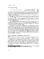
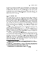
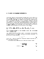
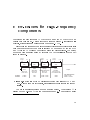
Every particle - elementary or composite - can be attributed to one of two groups.
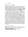
It can either be a boson or a fermion. Let us take a look at gure 1.1. On the
left hand side, a schematic of a gas at say room temperature in a harmonic trap is
shown. In quantum mechanics the eigenstates of such a trap can now be calculated
yielding equally spaced energy levels for a one-dimensional model, indicated by
the horizontal lines. For a classical gas the available states are sparsely populated
according to the Boltzmann distribution given by:
Ni =
1 −Ei /kB T
e
Z
(1.1)
where Ni denotes the number of particles within a sample in P
the i-th state with
an eigenenergy of Ei at temperature T in a sample of N = i Ni atoms. Z is
some normalization constant (in statistical mechanics: partition function) and kB
is Boltzmann's constant.
Cooling this sample down to very low temperatures while at the same time
increasing the density will, at some point, lead to the appearance of quantum
properties. For bosons the probability for the common occupation of one single state is increased compared to classical particles, satisfying the Bose-Einstein
distribution given in equation (1.2), where µ denotes the chemical potential.
Ni =
1
e(Ei −µ)/kB T
−1
(1.2)
This enhancement leads to a macroscopic occupation of the ground state for high
phase space densities, i.e. low temperatures paired with high densities. This phase
is called Bose-Einstein condensate (BEC) and has been predicted as early as in
1924 by Satyendranath Bose and Albert Einstein [1, 2, 3]. In 1995 nally the rst
1
Chapter 1 Introduction
pure1 BECs have been realized experimentally by Eric Cornell and Carl Wieman
at JILA [4] and Wolfgang Ketterle at MIT [5].
Bose-Einstein Condensate
Classical Gas
23
Na
Y(x)
ons
Bos
Degenerate Fermi Gas
Ferm
ions
6
Li
Decrease Temperature,
Increase Density!
Cooling down a gas leads to the appearance of quantum properties.
See text for more details.
Figure 1.1:
Fermions on the other hand must not occupy one single quantum mechanical
state. This is manifest in the Fermi-Dirac distribution, the analog to the aforementioned Bose-Einstein statistics:
Ni =
1
e(Ei −µ)/kB T
+1
<1
(1.3)
This has rst been claimed by W. Pauli in 1925, known as Pauli's principle. Ultimately the fermions will reduce the system's energy when cooled down by occupying the lowest empty states available. This leads to a sharp transition between
occupied and empty states at a certain energy level, known as the Fermi energy.
This phase is referred to as a degenerate Fermi gas.
There are two more essential principles for an understanding of quantum gases.
First in 1940 Wolfgang Pauli could show that the spin of a particle determines its
quantum properties [6]. Bosons carry integer spin, whereas fermions have halfinteger spin. The behavior of atoms as a whole is determined by the number of
electrons, protons and neutrons in its nucleus and shell, each contributing spin
1/2. Thus for odd numbers like in 6 Li (3 + 3 + 3) atoms are fermionic and for
even numbers like in 23 Na (11 + 11 + 12) they show bosonic behavior. Second, in
The transition to the superuid phase of 4 Heor type I superconductivity are Bose-Einstein
condensed systems, but strong interactions between particles complicate these systems heavily.
Strong interactions result in a reduced fraction of condensed atoms (about 10% in superuid
4
He).
1
2
1.1 Quantum Statistics - Bosons and Fermions
a regime in which quantum properties play a role, particles do no longer behave
like classical point-like particles but also show wave-like properties. This was rst
postulated in 1924 by L.V. de Broglie who attributed a wavelength
λdB =
h
p
(1.4)
to a particle of momentum p [7]. These properties are only relevant if the inner structure of the particle is small compared to its wavelength, since otherwise
particle-particle interactions are mainly arising from the interaction of electronic
shells. A second point is, that the inter-atomic distance needs to be on the order
of this wavelength. Or in other words:
nλ3dB > 1
(1.5)
where n is the number density. In statistical quantum mechanics this product
is also called phase space density or degeneracy parameter. This already gives
a rough estimate for temperatures needed in a system of given number density
n to observe eects arising mainly from quantum statistics. Therefore, we are
inserting equation (1.4) into equation (1.5). Using that the particle density n in
an ideal gas is given by n = P/(kB T ), where P denotes the pressure, yields a
critical temperature on the order of:
TC ≈
h2 n2/3
2mkB
(1.6)
This temperature is referred to as critical temperature for bosons2 and Fermi temperature for fermions. Yet for a rst estimate equation (1.6) is sucient. Typical
densities in experiments with cold atoms are on the order of 1014 atoms/cm3 . The
molar mass of 6 Li is 6 g/mol. This yields temperatures on the order of 1 µK.
Comparing this to a degenerate gas of electrons in a metal gives rise to a factor
of 104 (mass ratio) plus another six orders of magnitude (density ratio ≈ 109·2/3 ),
thus an overall factor of about 1010 in temperature, equivalent to temperatures
on the order of 10000K! So one could ask: Why should one be interested in such
hard-to-create systems? We would like to motivate this in the next section.
A more accurate analysis yields another factor of 2.612 in phase space density for spinless
atoms, resulting in temperatures that are about a factor of two lower. Corrections due to
interactions turn out to be small.
2
3
Chapter 1 Introduction
1.2 Degenerate Fermions
Bose-Einstein condensation has been a very active eld of research during the last
12 years. In the meantime there are approximately 60 BEC experiments in the
world3 that have accumulated extended knowledge about laser and evaporative
cooling, interactions in ultracold samples and BECs in a wealth of dierent geometries and potentials. BECs have been put into double-wells [8, 9], lattices [10],
eective two-dimensional structures [11], have been rotated [12] ... Yet there is still
a lot of exciting physics to be done. Common to them all is, that these systems
can be well described theoretically as described briey in section 1.2.2.
One research area that has developed recently and that we would like to join,
is the creation of degenerate Fermi gases of neutral atoms (DG). The rst such
DG gas has been observed in the group of Deborah Jin at JILA in Boulder in 1999
[13, 14]. Since then, several groups have caught up. A short overview on current
research topics and involved groups will be given in section 1.2.3.
There are now various reasons making research on DG so exciting. Ultracold
degenerate Fermi gases are a model system for nearly any strongly correlated
fermionic system. Quarks in a quark-gluon plasma, electrons in solids or neutron
stars may serve as examples. These systems have in common that many aspects
have not yet been captured theoretically and only now theorists are developing
methods that are able to treat many-body systems of fermions since perturbation
theories break down in this case (refer to section 1.2.2 for some remarks on this).
An important advantage of such a system is that it is clean. Clean in this context
means that no perturbing interactions like for example in solids exist. There are
no electron-phonon interactions, no electrostatic interactions among electrons and
with the ionic cores of the lattice. However, the most important thing is that within
a sample of trapped ultracold fermions there are several tunable parameters that
do not exist in other systems such as density (by means of the restoring force within
the trap), temperature (one can stop cooling at any point), and even scattering
lengths. The latter has the most dramatic consequences and will be discussed in
the following.
1.2.1 Feshbach Resonances
Consider a sample of atoms containing dierent spin states4 of fermions. A priori
collisions between two atoms with dierent spin states will only happen if they
3
4
4
Source: http://www.uibk.ac.at/exphys/ultracold/atomtraps.html
We will come back to that point in section 1.3.
1.2 Degenerate Fermions
approach each other to some distance comparable to the diameter of the atoms
(i.e. several a0 ≈ 5 · 10−11 m, Bohr radius), that is much smaller than the interatomic distance (about 100 nm) in an ultracold gas. Thus collisions will happen
only rarely.
This changes drastically if a magnetic eld is applied and tuned in the vicinity
of a so-called Feshbach resonance [15]. These resonances lead to scattering lengths
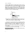
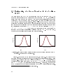
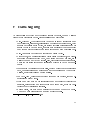
a that exceed by far the geometric extensions of the bare atoms. In gure 1.2 a
plot of the Feshbach resonances for a pair of 6 Li atoms of opposite spin is given.
There are two known Feshbach resonances at relatively low magnetic elds, a very
narrow one at 543 G and a very broad one at 837 G. The latter will be used in our
experiment since it demands only little accuracy when ramping magnetic elds.
Moreover one can even choose whether the particles eectively attract (a < 0) or
repel (a > 0) each other.
Scattering Length [a0]
6000
4000
2000
0
400
800
1200
-2000
-4000
-6000
Magnetic Field [Gauss]
Scattering length a in units of the Bohr radius a0 for Li atoms with
opposite spin as a function of the magnetic eld [16]. There are two Feshbach
resonances, at 543 G (not resolved in this plot) and 837 G, and a zero crossing of
the scattering length at 528G for the two lowest hyper-ne states in high elds.
For a > 0 the interaction is repulsive, otherwise attractive.
Figure 1.2:
6
We cannot give a detailed introduction to Feshbach resonances in this work, so
let us just motivate where they are arising from. For a nice introduction refer to
[17].
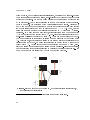
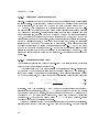
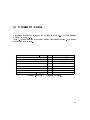
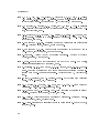
In gure 1.3 potential curves for two molecular states of dierent total angular
momentum (e.g. lowest two hyper-ne states in high eld) as a function of the
inter-atomic distance are plotted. The dashed line corresponds to the kinetic
energy of the unbound particles in the center of mass system. The oset arises from
5
Chapter 1 Introduction
the dierent hyper-ne states in the molecule. Dierent magnetic moments of the
two spin states allow for shifting the upper potential curve relative to the lower one.
Preparing the atoms in the open channel (the lower curve), i.e. in an unbound state
yields a coupling to the closed channel (upper curve) by means of spin exchange
collisions of the nuclear spin. If ever the kinetic energy is close to an energy level of
the closed channel the eigenstates repel each other (avoided transitions), leading to
a drastically increased scattering length5 . Thereby a lowering (increase) in energy
is equivalent to an attractive (a repulsive) interaction.
energy
potential of
molecular state
energy of incident
particle
potential for
two free atoms
inter-atomic distance
Schematic of potential curves for two molecular states of dierent total
angular momentum as a function of the inter-atomic distance; dashed line: kinetic
energy of the involved particles in the center of mass system.
Figure 1.3:
At suciently low temperature this leads either to Cooper pairing (for negative
scattering lengths) or molecule formation (for positive scattering lengths). This
situation is often referred to as BEC-BCS cross-over, since on the one side of
the resonance molecules are condensed into a molecular BEC (described by BEC
theory) on the other side bosonic Cooper pairs described in the BCS6 -theory of
superconductors.
For completeness we mention that there are also Feshbach resonances for pwave scattering of two atoms in the same spin state [19].
This system can be treated similarly to an atom in a light eld, using a dressed state approach
[17]. See also [18] for a nice introduction.
6
Bardeen, Cooper and Schrieer
5
6
1.2 Degenerate Fermions
1.2.2 Theoretical Approaches
1.2.2.1
BEC Theory
The inner structure (electronic conguration, magnetic and electrostatic properties) of species usually used in cold atom experiments is well known. Using this
knowledge collisions involving two atoms can be described theoretically. In cold
atom experiments with atomic velocities on the order of millimeters per second
the collisional energies are weak compared to the binding energies of the innermost
shells. Thus only valence electrons contribute. Two-particle interaction - featuring scattering and formation of molecules - of atoms is well understood and the
Schrödinger equation can be solved numerically.
However, moving to higher atom numbers quickly exceeds any available computer powers. Furthermore already three classical(!) particles (e.g. two planets in
a solar system[20]) may behave chaotically and solving such problems exactly is
impossible. On the other hand the exact solution of the Schrödinger equation of
say 106 cold atoms cannot be examined in an experiment anyway. One is rather
interested in macroscopic quantities that can be determined in an experiment like
for example densities, temperature, correlations between observables or maybe the
distance and radius of vortices in a superuid system.
As discussed before, bosons in a BEC occupy the same quantum mechanical state. Thus a simple and widely used approach is to reduce the N particle
Schrödinger equation to an eective one-particle one in a mean-eld approach:
~2
∂
2
∆ + Vext (~r) + g |Ψ(~r, t)| Ψ(~r, t)
(1.7)
i~ Ψ(~r, t) = −
∂t
2m
Here Vext denotes some external potential, N is the particle number and g is the
coupling constant that is proportional to the scattering length, thus positive for
repulsive and negative for attractive interactions. Mean-eld in this context means
that one assumes the other atoms to be homogeneously distributed in space, creating a net background eld corresponding to the last term of the Hamiltonian.
This equation was rst derived by Gross [21, 22] and Pitaevskii [23] in 1961 and
is called Gross-Pitaevskii equation (GPE). The non-linear term in the Hamiltonian assumes the interaction of the particles to be point-like. Only two-body
s-wave scattering processes are taken into account. This is justied if the temperature is low enough and higher order scattering freezes out and if the inter-atomic
distance is big compared to the scattering length such that three-body collisions
do not occur. For attractive interaction the non-linear term will decrease the total
energy of the system and thus lead to an increased particle density7 n and vice
7
2
Note that n ∝ |Ψ(~r, t)| , where n is the particle density.
7
Chapter 1 Introduction
versa. Using this, many phenomena can be described in Bose-Einstein condensed
systems. If needed, higher order interactions can be integrated into this model.
1.2.2.2
Strongly Coupled Fermions
A more interesting point and a currently very active eld of research is the description of strongly coupled fermionic systems. Evidently, an approach similar to the
GPE can not exist, since fermions have to occupy orthogonal quantum mechanical
states with an overall antisymmetric wave function. As long as they are weakly
interacting perturbation theoretical approaches still hold. However, the most exciting physics takes place right on and next to Feshbach resonances where the
systems are strongly interacting. Directly on a Feshbach resonance the scattering
length diverges and systems are supposed to show a unitary behavior, i.e. they
show the same characteristics on all length scales (in quark-gluon plasma but also
in neutron stars).
One method currently developed at the Theoretical Institute of the University
of Heidelberg [24, 25] is a quantum eld theoretical approach called Functional
Renormalization (FR). In quantum eld theory [26] one typically encounters
divergences for high momenta (i.e. small distances). These arise from a breakdown
of the continuum description of elds8 . However, this problem can be solved by
introducing a so-called ultraviolet cuto and replacing higher momentum physics
by measured quantities. For quantum eld theory a small number of measured
quantities like for example the electron's mass and charge are needed. However,
this allows for quantitative predictions of physical observables. Whenever such
an approach is feasible, the corresponding theory is called renormalizable. In a
next step, the known action on a microscopic scale is extended to an eective
action on a macroscopic scale. Since FR is not based on perturbation theory it
can be used for the description of strongly correlated systems. The outstanding
point about ultracold gases is now, that the microscopic behavior of these atoms
is very well known - in contrast to for example in high energy physics. Taking this
as a starting point and extending this to a macroscopic scale yields macroscopic
observables (e.g. relations between correlation lengths and core sizes of vortices).
A complementary method is Quantum Monte-Carlo simulation. See [27]
for a very detailed review and [28] for a more recent example on degenerate Fermi
gases close to a Feshbach resonance. Basically, one uses some quantum mechanical model (e.g. many-body Schrödinger equation, path integral formalism) as a
starting point and denes some initial wavefunction. Then random walks are used
This is in some way comparable to the UV catastrophe in Rayleigh-Jean's law, where a
discrete description needs to be applied for high photon momenta.
8
8
1.3 Why Lithium
AND Sodium?
for solving (path) integrals or for consecutive steps in phase space.
1.2.3 Current Research Topics - A Short Summary
In this section we would like to give a short overview on current research topics in
the leading groups of the international community. This list does not claim to be
complete.
• In the group of Deborah Jin at JILA p-wave Feshbach resonances are
examined [19].
• The groups of Randy Hulet, Rice University [29] and Wolfgang Ketterle,
MIT [30] deal with imbalanced spin mixtures and explore phase diagrams in
such systems.
• At Duke University the group of John Thomas investigates thermodynamics at a Feshbach resonance [31].
• The group of Rudi Grimm, University of Innsbruck is doing spectroscopy
[32] on ultra-cold degenerate Fermi gases and examines their dynamics [33].
• In the group of Christophe Salomon, ENS the transition from a gaseous
to a crystalline phase is investigated [34]. Recently expansion experiments
have been done [35].
1.3 Why Lithium AND Sodium?
We have chosen fermionic 6 Li and bosonic 23 Na for our experiment. But why a
bosonic part if all this is about fermions? Even though there is in fact interesting
physics [36, 37] when dealing with a mixture of a degenerate Fermi gas and a BEC,
this mainly has to do with our cooling strategy. In a rst step laser cooling is done.
Yet to reach temperatures below the critical temperatures this is not sucient,
since only temperatures on the order of hundreds of µK can be achieved for lithium.
In BEC physics evaporative cooling [38] is done. Thereby the fastest atoms are
removed. Ecient cooling is only achieved if collision induced rethermalization
occurs suciently fast. These collisions are mainly s-wave scattering processes,
since higher order collisions freeze out at the given temperatures. During this step
the atoms are typically trapped in a magnetic trap9 , thus the sample is usually
There are groups with "all optical" setups [39]. In this case atoms are transferred from the
MOT to an optical dipole trap directly and this problem does not arise. But for this enormous
laser powers (typically several tens of watts) are needed for achieving suciently high potentials.
9
9
Chapter 1 Introduction
spin polarized. The important point about spin-polarized fermions is now, that
s-wave collisions are forbidden by Pauli's principle for low temperatures, while
higher order collisions are freezing out. Consequently thermalization would slow
down drastically for decreasing temperatures.
As collisions between dierent spin states are still allowed at low temperatures,
cooling down to degeneracy can be done by using dierent spin states. In fact, this
has been the rst working solution ever and was chosen by the group of Deborah
Jin at JILA. Disadvantageous is that one loses about 99% of the atoms. This can
be circumvented using a second approach, called "sympathetic cooling" [40]. It is
based on creating a conventional BEC of bosons and during this cooling process
using the bosons as a refrigerant for the fermionic component. An important
advantage is that the atom number of fermions decreases only slightly.
1.3.1 General Aspects
During the last few years several groups have already reached Fermi degeneracy
with dierent approaches and various combinations of elements [14, 41, 42, 43].
This section is meant to be an overview on dierent isotopes used together with a
brief discussion of their pros and cons.
Common to nearly all of these experiments is, that either 6 Li or 40 K are used10 .
Alkalis have in common that their level schemes are simple11 and well understood.
6
Li and 40 K (half life time 109 years12 ) are the only stable alkaline fermionic isotopes. Both show Feshbach resonances (see section 1.2.1 for details on 6 Li ) at
reasonable magnetic elds. However, 6 Li oers a resonance with a width of about
100G whereas in 40 K the widths on the order of one Gauss can hardly be resolved
[45]. Another point in favor of 6 Li is that molecules formed in the vicinity of a
Feshbach resonance have higher lifetimes [46, 47]. On the other hand 40 K has a
resolved hyper-ne structure in the excited state (thus better laser cooling is possible, see section 2.2.4). Advantageous about 40 K is also that its vapor pressure
is much higher at a given temperature than for Lithium. The magneto-optical
trap (cf. 2.2) can thus be loaded from the background pressure created by a small
dispenser whereas a high temperature oven needs to be used for 6 Li.
Once the fermionic part is chosen, the choice of bosons is reduced taking into
account that for optimal heat transfer, the masses of the two species should not
Recently the group of Yoshiro Takahashi achieved Fermi degeneracy with (exotic) Ytterbium
(Yb), oering two stable fermionic and ve stable bosonic isotopes, all with reasonable natural
abundance [44]. We will restrict our discussion to the aforementioned elements.
11
They are hydrogen-like with only one electron in the outermost shell.
12
data from http://atom.kaeri.re.kr/ton/
10
10
1.4 Outline
dier too much. The same condition holds for magnetic trapping (cf. section
3.4.2), as for dierent masses the centers of the trap for the dierent species are
shifted slightly due to the gravitational force (also called gravitational sag). This
impairs their heat contact. The bosonic counterpart should not be lighter than the
fermions. As seen in equation (1.6) the critical temperature decreases for increasing
mass. As a consequence, the deeper one wants to cool into degeneracy, the lighter
the fermion should be relative to the boson. Additionally one needs a suciently
large thermal bath, for the desired size and temperature of the fermionic sample.
Finally, the inter-species collisional properties are of importance, however, they
are generally not predictable and have to be acquired experimentally. Resuming
the previous arguments, mainly four combinations are reasonable and used 7 Li /
6
Li (e.g. in the groups of Hulet, Rice and Salomon, ENS), 87 Rb / 40 K (e.g. in
the groups of Bloch, Mainz and of Inguscio, Florence) and 7 Li / 23 Na (group of
Ketterle, MIT) and 6 Li / 87 Rb (e.g. in the group of Zimmermann, Tübingen).
1.3.2 Our Motivation for Choosing Lithium and Sodium
We chose 6 Li mainly for its broad Feshbach resonance that can easily be resolved.
So the creation of a suciently homogeneous magnetic eld all over the entire
atomic cloud is feasible. As a last point 6 Li is readily available13 .
23
Na was chosen because it is only slightly heavier (as discussed before) and
the biggest BECs ever have been realized with sodium [48]. Our Zeeman slower
can be used for both species with sucient eciency (see 3.3.1). Last but not
least, there are successful experiments running with 23 Na and 6 Li [49]. So we will
not have to deal with problems that have not been solved before as the target of
the experiment is to reach degeneracy as soon as possible.
1.4 Outline
On our way towards a degenerate gas of ultracold 6 Li atoms and a BEC of 23 Na
mainly a vacuum system and a laser system need to be set up. Atoms are evaporated in two high temperature ovens, slowed down, trapped and cooled using
magnetic elds and lasers. For sodium there are no solid state lasers available at
present and dye lasers need to be used. The outline of this thesis is as follows:
The natural abundance of 6 Li is about 7%, whereas the rest is 7 Li , we use enriched lithium
containing about 95% 6 Li ; The natural abundance of 40 K is only about 0.012% and is mainly
won in nuclear power stations.
13
11
Chapter 1 Introduction
In chapter 2 we will give an introduction to dye lasers to an extent that seemed
to be necessary to understand the specic properties - also problems - of our laser
system. Another point we would like to touch upon in this chapter is some theory
on magneto-optical trapping.
Chapter 3 will give an overview on what has been set up in the rst year of
this experiment. We will describe the vacuum system, the Zeeman slower and the
magnetic coils briey before giving a more extensive description of the laser system
that has mainly been developed and set up under the author's responsibility during
the rst months.
In part 4 we will present rst measurements of the properties of our magnetooptical trap for sodium atoms.
The appendix nally contains some sodium data and several important experimental tools realized during this diploma thesis - namely a beam proler based
on a webcam, a microcontroller based atomic shutter driver for our vacuum apparatus, the spectroscopy cell for Doppler-free saturated spectroscopy of sodium and
the driver electronics for high frequency modulators.
12
2 Theory
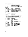
2.1 Dye Lasers
We use a laser system based on two Radiant Dyes Dye Ring Lasers. For sodium
and lithium we chose rhodamine 6G (R6G) and DCM (4-Dicyanomethylene-2methyl-6-(p-dimethylaminostyryl)-4H-pyran) respectively. In the following we will
concentrate on our laser for sodium, however, the results are generic for nearly all
dyes. In section 2.1.1 some laser basics needed in the subsequent chapters are
given. In section 2.1.2 some special features of dyes are discussed. Finally, in
section 2.1.3 we will show how to achieve single mode operation of a dye laser at
a desired wavelength, introducing the mode selective elements in a dye ring laser.
2.1.1 Some Laser Basics
This section is not meant to be a profound introduction to laser physics. The
aim is to recall some laser basics that will be needed in the following. For further
details refer to any standard text book, e.g. [50] for a general introduction, or
[51, 52] for specic questions on dye lasers. The rst working laser a ruby laser
was built in 1960 by Theodore Maiman1 . Six years later the rst dye laser was
invented by chance in the group of Fritz P. Schäfer [53]. Examining the saturation
characteristics of cyanine, the reectivity of about 4% of a polished cuvette was
sucient to enable lasing.
Prerequisite for the construction of a laser is an active medium amplifying incoming light coherently (i.e. same phase and wavelength). Therefore, a population
inversion needs to be achieved, since only then stimulated emission dominates the
absorption in the gain medium. This cannot be achieved in thermal equilibrium or
in a system of only two levels2 , since Boltzmann's factor cannot exceed 1. In appropriate systems of three and four levels, this becomes possible. A key feature of
1
2
see http://www.pat2pdf.org/patents/pat3353115.pdf for the original patent
Strictly spoken this holds only on timescales bigger than the natural linewidth.
13
Chapter 2 Theory
these media is, that the laser transition's lifetime, constituted of all non-coherent
decay channels (spontaneous emission, non-radiative decay) is long compared to all
other decay processes. Let us have a look directly at the level scheme of rhodamine
6G in picture 2.1, that will be discussed in some more detail in the next section.
Refer to gure 2.1 for notations of the various lifetimes and states. Lifetimes τ2
and τ4 are on the order of picoseconds or even sub picoseconds (see next section
for a brief justication) and very small compared to τ3 ≈ 0.1 µs. Thus, one can
assume in a simple approach that all electrons excited to h2i decay into h3i instantaneously. In a rst step pumping light excites electrons from the ground state
h1i to any sublevel of the excited state h2i3 . Non-radiative transitions (induced by
non-elastic collisions) populate the state h3i. There are now several decay paths.
The most desirable is stimulated emission to some sublevel of the ground state
h4i. Furthermore, spontaneous emission to the ground state or transitions to the
triplet states may occur. In a last step electrons in energy level h4i relax to the
ground state h1i. Taking into account the absorption of the pump beam, stimulated emission and spontaneous emission as well as all non-radiative processes,
one can establish rate equations allowing to calculate the lasing threshold (i.e. the
pump power needed for lasing) and the time dependent behavior.
S2
T2
S1
<2>
s emis
excitation sS
T1
n e ou
t3
tT
sion
stim. emission s em
t 3,T
sponta
<3>
S0
Absorption sT
t2
<4>
<1>
t4
Term scheme of rhodamine 6G, S denotes electronic singlet states, T
the corresponding triplet states
Figure 2.1:
3
14
Evidently h2i and h4i may be any state within the upper and lower band.
2.1 Dye Lasers
A last important property of dye lasers is, that in steady state operation dye
lasers with electrons occupying only one single excited state (all electrons in h3i)
will run in a single longitudinal mode at every time (though fast mode hops may
occur leading to an eective multi-mode operation). This is due to what is called
homogeneous line broadening of the gain medium. Electrons in h3i serve as a
reservoir for all possible longitudinal modes. As a consequence, only one mode at
a time will be amplied at the expense of all the others. Stimulated emission within
the gain medium amplies the longitudinal mode with wavelength λ and intensity
∝ N3 ·I(λ), where N3 denotes the density of electrons in the
I(λ) according to dI(λ)
dt
h3i state. Hence, the most intense mode depopulates electrons in the h3i state the
most and prevails the others, that gain less gradually and get damped out by losses
within the cavity. In case dierent longitudinal modes are amplied by dierent
reservoirs of excited electrons, i.e. they do not compete, the gain media are called
inhomogeneously broadened (for example Doppler broadening in gas lasers).
2.1.2 The Ring Dye Laser
In general, dye molecules consist of a large number of atoms. This leads to a big
number of dierent vibrational degrees of freedom (50 atoms give rise to about
150 vibrational modes). Many of these vibronic excitations directly couple to the
electronic transitions, adding sublevels to these spectra with typical mode spacings
of approximately 1 THz to 100 THz. Additionally rotational degrees of freedom
come into play with a mode spacing of typically 10 GHz to 1 THz. These levels are
strongly broadened due to collisions with the solvent, yielding a quasi-continuous
absorption spectrum. Furthermore, the band structure depends on temperature,
dye concentration and acid-base equilibria with the molecules of the solvent.
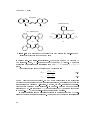
There are mainly three generic classes of dye molecules (cf. gure 2.2). However,
common to all of them is the presence of several conjugated double-bonds (a so
called system of π -electrons). In a simple approach, one can assume the electrons to be in a constant box potential within this system of conjugated doublebonds. One distinguishes linear systems (e.g. pinacyanol), circular systems (e.g.
Cu-Phtalocyanin) and more complicated branched systems like in the case of rhodamine 6G. For linear molecules the eigenenergies of the n-th eigenstate then
reads:
h2 n2
(2.1)
En =
8mL2
where h is Planck's constant, m is the electronic mass and L is the length of the
box potential. For ring-like structures the same equation holds, however, there
are two eigenstates to each eigenenergy (there are no xed boundaries, resulting
15
Chapter 2 Theory
Pinacyanol
+
N
N
C2H5
C2H5
Rhodamine 6G
COOC2H5
Cu - Phtalocyanin
H3C
CH3
N
H5C2
N
N
N
N
Cu
N
NH
O
+
Cl
NH
C2H5
-
N
N
Left: Structure of two generic dyes with a linear and ring-like shape
[51]; Right: Structure of hodamine 6G [54]
Figure 2.2:
in distinct sine- and cosine-like solutions). Every state can now be occupied by
two electrons. Thus, N π -electrons occupy the lowest N/2 states. The lowest
absorption band arises from transitions from the n = N/2 to the n = N/2 + 1
state.
The corresponding energy dierence and wavelength is:
h2 (N + 1)
(2.2)
8mL2
8mc L2
(2.3)
λmax =
h N +1
where c denotes the speed of light. In R6G rough estimations of the absorption
wavelength are no longer that easy as it is neither linear, nor circular but there are
several connected circles of π -electrons. However, for R6G-molecules the qualitative behavior described above still holds. In gure 2.2 one can nd the chemical
structure of R6G. Its absorption σs (λ) and uorescence Φ(λ) spectrum is depicted
in gure 2.3. σem (λ) is the cross-section for stimulated emission.
In a liquid solution large molecules experience in general more than 1012 collisions with solvent molecules per second. This means that the system reequilibrates
Emin =
16
2.1 Dye Lasers
Fluorescence Φ(λ) and absorption σs (λ) spectrum of a rhodamine 6G
solution (10−3 mol−1 ). The data is based on measurements of Fuh et al. 1998 [55].
Knowing the lifetime of the excited state, one can calculate the cross section for
stimulated emission σem (λ) (for more details: cf. [56]). An approximate curve for
triplet state absorption σT (λ) has been inserted.
Figure 2.3:
on the order of picoseconds at room temperature ending up in the vibronic ground
state of the rst excited electronic state (or in any higher state according to Boltzmann's distribution).
The emission spectrum can now be obtained by mirroring the absorption spectrum around the frequency of the purely electronic transition. Absorption excites
electrons from the electronic and vibrational ground state to any excited electronic
and vibrational state, emission starts in the electronic excited state and vibrational
ground state to any vibrational state of the electronic ground state (see gure 2.1).
Up to now, we did not take triplet states into account. For every electronic
excited singlet state there is a corresponding triplet state. One can show with
a simple argument that triplet state energies are inferior to the corresponding
singlet state energies. The overall wave function for a system of two electrons in
states m and n, at positions r1 , r2 and with spins s1 , s2 needs to fulll Pauli's
principle, i.e. the total wave function needs to be antisymmetric toward particle
exchange. There are now two dierent possibilities: Either spins are parallel or
antiparallel to each other leading to a symmetric or antisymmetric spin function.
As a consequence, the corresponding wave functions needs to be antisymmetric or
17
Chapter 2 Theory
symmetric, respectively.
ψs = ψm,n (r1 , r2 ) + ψn,m (r1 , r2 )
ψas = ψm,n (r1 , r2 ) − ψn,m (r1 , r2 )
symmetric wave function
antisymmetric wave function
(2.4)
(2.5)
Symmetry now leads to electrons being closer to each other than in the asymmetric
case leading to a higher potential energy. Thus, triplet state energies are always
lower than the corresponding singlet states and transitions occur, mediated by
collisions with the solvent!
Figure 2.1 shows the relevant level scheme of rhodamine 6G. Optical pumping
with green light (e.g. 515nm or 532nm) excites electrons from the S0 ground state
to a substate of S1 . By means of non-radiant processes (collisions with solvent
molecules) electrons occupy the lowest S1 state h3i - with h1i, h2i, h3i and h4i
forming a four-level system.
There are several loss processes intrinsic to the gain medium. First of all
spontaneous emission from h3i to h4i and collisions inducing transitions to T1
depopulate the upper laser level. Moreover absorption of laser light to T2 is actively
damping the laser beam within the cavity.
Concluding, the most important principles of Dye Lasers are that to a good
approximation the energy levels h2i are empty whereas h3i is populated by means
of the pumping light. However, there are actually collision induced losses to the
triplet state absorbing lasing light, thus, at a certain point higher pumping powers
do not yield any higher output powers, but saturate. Furthermore, the dye liquid
may heat up locally leading to instable laser operation. Both eects can be reduced
using a dye jet, such that dye transferred to the triplet state is quickly removed
out of the laser. As a rule of thumb the higher the speed of the jet the higher the
pumping power can be chosen4 .
2.1.3 Singlemode Operation of Dye Lasers
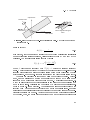
In this section, the dye laser we use will be described. In gure 2.4 one can nd
a schematic overview of our ring dye laser manufactured by Radiant Dyes Laser
& Accessories GmbH. All elements are mounted onto an invar bar for minimal
thermal expansion of the cavity. Central feature is a polished nozzle of optical
quality ejecting a thin lm of dye solution (in the following referred to as dye
jet) through the cavity into a catcher hose. The pressure needed is provided by
a Radiant Dyes dye circulator pushing the dye solution through the dye nozzle at
up to 7 bar.
For our system saturation starts at about 7 W of pumping power for 6 bar of dye pressure.
However, stable single-mode operation is only possible up to about 6 W.
4
18
2.1 Dye Lasers
Figure 2.4:
Dye Laser
Overview on our ring dye laser, source: Manual for Radiant Dyes Ring
As a pump laser we use a Radiant Dyes MonoDisk5 laser, which is a frequency
doubled, diode pumped Yb:YAG ring laser emitting two laser beams of >10W each
at 515 nm. This is due to the absence of an optical diode enabling two counterpropagating beams to persist. The active medium is inhomogeneously broadened
permitting two dierent non-competing longitudinal modes.
One of the two outputs is focused onto the dye jet by Mirror Mp. Mirrors M1,
M2, M3 and M4 are forming the cavity. M1 and M2 are concave mirrors with a
radius of curvature r = 150 mm focusing the intracavity laser beam onto the dye
jet.
2.1.3.1
Optical Diode (OD) and Thin Quartz Plate
In order to avoid competing counterpropagating beams an optical diode (also called
Faraday isolator) is inserted into the cavity introducing additional losses for beams
directed from M3 to M4. All optical elements made of glass (except for the etalons)
are brought into the cavity under Brewster's angle. This induces losses for modes
with polarization perpendicular to the laser plane. The quartz plate (i.e. λ/2plate) rotates the polarization by 45◦ . Within the Faraday rotator (Faraday active
crystal combined with a strong permanent magnet), the original polarization is
restored for a beam traveling in the desired direction, but it is turned for a counterpropagating beam, which then suers losses on subsequent circulations. As
discussed in the previous section the mode with the highest gain per circulation
will prevail - inhibiting counterpropagating beams.
5
A modied ELS "MonoDisk" laser.
19
Chapter 2 Theory
2.1.3.2
Selecting a Longitudinal Mode
Single-mode lasers that can be tuned close to an atomic resonance are a prerequisite
for laser cooling. Their frequency accuracy needs to be smaller than the natural
atomic linewidth, so for example 1 MHz in the case of sodium (line width Γ =
2π · 10MHz). This corresponds to a relative frequency accuracy of about 10-9 .
Simultaneously the tuning range of the gain medium (several tens of nanometers for
R6G) should be conserved. It is intuitively clear that this is not feasible with only
one optical element, as there has to be a tradeo between the free spectral range
(FSR, the frequency distance between two transmitted modes), the width of the
transmission peak and the tunability. Instead several hierarchic lters are inserted,
namely a birefringent lter, a thin and a thick etalon and, nally, the resonator
itself that can be tuned by a tweeter and a galvo plate. These elements provide
wavelength selectivity on scales of several nanometers (i.e. THz) to the order
of MHZ in the order mentioned above. The product of the transmission proles
results in a sharply peaked curve permitting to suppress all but one mode. These
elements will be described briey in the following. Their assembly is sketched in
gure 2.4.
2.1.3.3
Birefringent Filter (BR)
The birefringent lter is composed of a three-staged Lyot lter [57] with a thickness
ratio between two subsequent lters of two.
The easiest case of a Lyot lter consists of a birefringent plano-parallel plate
of thickness d (the optical axis lying inside the plane) followed by a polarizer. A
laser beam hitting the surface perpendicularly, with a linear polarization angled
45◦ to the optical axis, may pass without any polarization changes if the condition
or:
kne − no k d = N λN
Nc
!
f (d, N ) =
kne − no kd
(2.6)
(2.7)
is fullled. Here N is an integer, ne and no denote the extraordinary and ordinary
refractive index respectively, thus, kne − no kd is the dierence between the optical
path lengths within the crystal. If this dierence is equal to a multiple of the
wavelength N λN no phase shift will happen. Light with a frequency satisfying
equation (2.7), that has been derived using f = c/λN (c: speed of light), passes
the plate without any polarization changes.
Putting a polarizer behind the crystal transmitting the incident polarization,
all frequencies given by equation (2.7) can pass through freely. The free spectral
20
2.1 Dye Lasers
Birefringent Plate
Optical Axis
Rotation Axis
a
Laser Beam
b
Laser Beam
Three-stage Birefringent
Filter
Schematic of a three-stage birefringent lter. On the left one of these
stages is drawn.
Figure 2.5:
range is given by
∆f (d) =
c
kne − no kd
(2.8)
It is evident, that for all other wavelengths the outgoing polarization is elliptical
or in special cases circular or linear, yielding losses between 0% and 100% at the
polarizer. The overall transmission is given by [58]:
π (f − f0 )
2
T (f, d) = cos
(2.9)
∆f
where f0 denotes some frequency with T (f0 ) = 1 within the relevant frequency
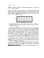
range. Concatenating several Lyot lters to the aforementioned three-staged birefringent lter results in narrower transmission peaks while conserving the free
spectral range. See gure 2.6 for plots of single and combined transmission curves.
The assembly discussed so far does not allow for wavelength tuning. Furthermore, one can realize such a lter more easily in the case of a dye laser or any
laser with a homogeneously broadened gain medium. As discussed in section 2.1.1
a very small percentage of additional losses is sucient for the suppression of a
mode in such a laser. Polarizers can be replaced by a plate under Brewster's angle.
Refer to gure 2.5 for an overview. The plates are no longer perpendicular to the
incident beam but are mounted rotatably and under Brewster's angle. Brewster
surfaces serve as polarizers introducing this slight but sucient loss on the perpendicularly polarized component. Another change is that the optical axis points out
of the plane, thus, the angle between incident beam and optical axis varies while
21
Chapter 2 Theory
1.0
0.8
0.6
Transmission
0.4
0.2
0
1.0
0.8
Df = FSR
0.6
0.4
df
0.2
0
f0-Df
f0-Df/2
f0
f0+Df/2
f0+Df
The upper gure shows transmission curves for Lyot lters with arbitrary thicknesses d (red, dotted line), 2d (violet, dashed line) and 4d (blue, solid
line). Below the overall transmission of a subsequent arrangement of these three
previous lters is shown. ∆f is given by the free spectral range of the thinest
plate ∆f (d0 )/2, the FWHM is approximately equal to the FWHM of the thickest
plate, i.e. ∼ ∆f (4d0 )/2
Figure 2.6:
rotating the birefringent lter. As a consequence, kne − no k can be changed and
the transmitted wavelength can be tuned. However, an important disadvantage of
a real birefringent lter is that one does not hit the ratio 2:1 perfectly well. As a
consequence, maxima do not overlap automatically for all wavelengths specied in
equation 2.7, but one has to rotate the Lyot lters slightly relative to each other
in order to get this close to ideal overlap for the desired wavelength range. For
a more detailed description refer to [58]. In our case the FSR is on the order of
several tens of THz.
2.1.3.4
Thin and Thick Etalon (TNE and TKE)
The birefringent lter discussed above allows for tuning across the gain width of
the dye, yet it is not suciently selective to achieve single mode operation. Now
we would like to briey present the function of the next levels in hierarchy, two
Fabry-Perot etalons called thin and thick etalon.
The thin etalon is a 0.5 mm thick glass plate at close-to-normal incidence with
coated surfaces for a reectivity of about
R=20%, yielding a FSR of about 200 GHz
1−R
π
and a nesse6 of F = 2 / arcsin 2√R ∼ 1.4. It can be tuned by slightly rotating
6
22
Ratio between free spectral range ∆f and FWHM of the transmission peaks δf (nomencla-
2.1 Dye Lasers
its mount that incorporates a galvanometer simultaneously. This leads to a slight
change of the optical path between the two surfaces and shifts the transmitted
wavelengths.
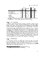
The thick etalon is composed of two adjacent prisms (cf. gure 2.7) with a
small distance between them, one of which is mounted onto a cylindrical piezo.
Wavelength tuning can now be done by changing the voltage applied to the piezo.
The inner surfaces are cut under Brewster's angle. The total thickness of the
system is about 10 mm resulting in a FSR of about 10 GHz, also with a nesse of
about 1.4.
10mm
cylindrical piezo
Figure 2.7:
2.1.3.5
Schematic drawing of the thick etalon, refer to the text for details.
Tuning Resonator Modes: Galvo/Brewster Plate and Tweeter
(GP and M2)
The mode spacing of the cavity is given by ∆f = c/l ≈ 200 MHz, where c denotes
the speed of light and l the resonator length of about one and a half meters. When
frequency sweeps are done this length needs to be adapted, since otherwise mode
jumps between dierent cavity modes would appear. This feature is provided by
the galvo plate (also called Brewster plate), a window brought into the resonator
that can be turned by means of a galvanometer. Turning the GP leads to the
desired changes of the resonator length as the optical path inside the plate (with
refractive index of approx. 1.5) changes. The tuning range of the GP exceeds
30 GHz, however, the mechanical inertia inhibits fast changes and especially cannot
compensate any fast uctuations of the resonator length. This is where the tweeter
(mirror M2 mounted onto a piezo) comes into play. It permits to change the
resonator length quickly (on the order of kHz), but only with a small amplitude
that corresponds to some hundreds of MHz.
ture like in 2.6). See any optics textbook for more details.
23
Chapter 2 Theory
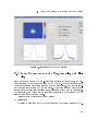
2.1.3.6
Locking the Laser to the Internal Fabry-Perot Cavity and Frequency Sweeps
Single mode operation at maximal output power is achieved, if all wavelength selective elements mentioned before are aligned such that their transmission maxima
overlap in order to minimize losses for the desired wavelength and to get a maximal
frequency selectivity (i.e. losses are substantially lower for exactly one longitudinal
cavity mode than for all the others).
Voltage [V]
4
2
0
-2
-3
-2
-1
0
1
Frequency [GHz]
2
3
Transmission curve of the reference cavity registered by the photodiode,
shifted to negative voltages such that locking can easily be done on any zero
crossing of the signal.
Figure 2.8:
How this overlap is realized in practice will be described in the following. First
the birefringent lter is manually tuned to the approximate mode. One can clearly
see mode hops of 200 GHz (FSR of the thin etalon) on a wavemeter while turning
the micrometer-screw. Afterwards the thin etalon oset allows to select the right
frequency to about 10 GHz, corresponding to the FSR of the thick etalon. The
nal position of the thin etalon is adjusted with a controller permitting to tune
the center frequency of the thin etalon to −15...+15 GHz. The center wavelength
to end up with is already now dened quite precisely. The remaining elements
(TKE, GP, tweeter) are synchronized electronically. Therefore, about 2× 1% of
the outcoupled beam are split o. One is directed onto a photodiode directly
(power signal), the other one passes through a temperature stabilized and tunable7
Fabry-Perot cavity with FSR of about 1 GHz and a nesse of 2, and is captured by
another photodiode. This signal (reference signal) is divided by the power signal
compensating any intensity uctuations.
The thick etalon locks one peak of the etalon transmission curve to the laser
wavelength. This is realized using a lock-in technique: The thick etalon is modulated with a low amplitude at a frequency of approximately 2 kHz yielding a
Inside the cavity there is another galvo plate that can shift transmission fringes by more
than ±15GHz
7
24
2.2 Magneto-Optical Trapping
frequency modulation of its transmission curve and an amplitude modulation of
the output power of the laser. The internal lock-in amplier generates the error
signal out of the power signal and feeds it back onto the TKE.
Galvo plate and tweeter are locked to the Reference cavity. Frequency locking
is now done on any positive slope of the transmission spectrum. This is why the
voltage level of the reference signal can be shifted to negative values (see gure
2.8 for a schematic). The zero-crossings dene lock-points. It is now sucient to
take the registered and shifted signal as input for the control loops of galvo plate
and tweeter.
Frequency scanning is simply achieved by scanning the reference cavity. A
feed-forward signal is put onto the thin etalon that is followed by the TKE. Galvo
plate and tweeter cancel any non-zero reference cavity signal and consequently
follow the sweep.
2.2 Magneto-Optical Trapping
In this section, the concept of magneto-optical trapping will be introduced briey.
After a short introduction to light forces on two-level atoms we want to provide a
basic understanding of how light forces can be used for cooling of neutral atoms.
In the last part this concept will be extended to the case of multilevel atoms,
where new eects like for example sub-Doppler cooling arise, always in view of the
specic situation in a sample of sodium and lithium atoms. Finally, the working
principle of a magneto-optical trap (MOT) will be described.
2.2.1 Light Forces on Two-Level Atoms
There are two distinct eects exerting forces on atoms. They are briey described
in the following. Note that only a classical motivation is given.
A quantum mechanical derivation can be found in the book of Metcalf and van
der Straten [59]. The way to go is to establish a Hamiltonian containing a term
coupling the eigenstates by means of a dipole operator to an electro-magnetical
eld. Diagonalization leads to the appearance of "new" eigenstates called dressed
states. Inserting these states into a statistical density matrix approach and introducing spontaneous emission leads to the optical Bloch equations describing the
time dependent behavior of these systems.
25
Chapter 2 Theory
2.2.1.1
Dipole Force
Here, this aspect is only given for the sake of completeness. However, an important
point for our future experiment will be the construction of an optical dipole trap
[60, 61] precisely based on the optical dipole force8 !
We would like to give a classical justication for this force. In a classical approach a two-level atom can be compared to a damped electrical resonator with
the resonance frequency ω0 and a dipole momentum of p~ driven by an inhomoge~ x, t) = E~0 (~x) cos(ωt). Solving the dierential
neous alternating electrical eld E(~
equation for a driven damped oscillator yield a phase dierence between eld and
oscillator of:
2βω
(2.10)
φ(ω) = arctan
ω02 − ω 2
Phase [°]
where β is the damping coecient. This equation is plotted in gure 2.9.
180
160
140
120
100
80
60
40
20
0
red detuning
blue detuning
w0-b w0
Frequency
Relative phase between a driven oscillator and the driving eld as a
function of detuning
Figure 2.9:
In electrodynamics the time averaged potential energy U of a dipole in an
electric eld is given by [62]:
~ x)
U (φ) = − cos(φ)~p · E(~
(2.11)
The qualitative behavior of U as a function of detuning can be deduced from
gure 2.9. For blue detuning − cos(φ) is positive, thus, the mean potential is
increased whereas red detuning lowers the particle's potential energy. Finally, the
~x-dependence of the electrical eld induces a dipole force.
~ (φ)
F~dip = −∇U
(2.12)
Concluding, a dipole in an inhomogeneous alternating eld is torn into the maximal
eld for red detuned (ω − ω0 negative) light but seeks low elds for blue detuned
8
26
Other names are reactive force, gradient force and redistribution force.
2.2 Magneto-Optical Trapping
light (ω − ω0 positive). For the conditions met in the aforementioned dipole trap
a quantum mechanical calculation (dressed state approach) gives the following
approximation:
~Γ2 ~
F~ = −
∇I(~x)
(2.13)
8δIs
where I(~x) denotes the laser beam intensity, Is the saturation intensity of the
transition and Γ the natural linewidth. δ is the laser detuning (δ = ω − ω0 ).
2.2.1.2
Light Pressure Force
Near and at resonance, also dissipative processes can be used for cooling. Whenever
an atom absorbs light it gathers a photon's momentum p~phot = ~~k . Once in the
excited state there needs to be some kind of deexcitation through spontaneous or
stimulated emission before a second excitation process can start. Consider now
the two possible processes: Absorption followed by stimulated emission does not
change the atom's momentum and will not serve for cooling since incoming and
outgoing photons are the same. Spontaneous emission, on the other hand, leads to
scattering of photons to random directions - thus, there is a mean net momentum
of N p~phot acquired after scattering N photons. This force is called light pressure
force9 However, since electrons in the excited state have a non-zero lifetime τ = 1/Γ
the rate of scattered photons is limited. It can be calculated using the following
equation [59]:
S
Γ
(2.14)
γscatter =
2 1 + S + 2δ 2
Γ
S = I/Is is called saturation parameter with the transition and polarization specic saturation intensity Is and δ denotes the detuning of the laser relative to the
resonance. In the limit of high saturation γscatter approaches Γ/2. This corresponds
to the situation that half of the atoms are in the excited state and spontaneous
decays happen at a rate of Γ. Even though the recoil of the atom when absorbing
one photon is only about 3 cm/s for sodium and lithium, the big linewidths of
Γ ≈ 2π · 10 MHz lead to accelerations on the order of |a| = 105 m/s2 !!
10
2.2.2 Optical Molasses
Up to now, we have neglected any eects arising from the movement of the atoms.
Moving atoms experience a Doppler shifted light frequency and thus, a velocity
9
10
This force is also known as scattering force, radiation pressure force and dissipative force.
Containing the laser detuning but also Zeeman or Doppler shifts.
27
Chapter 2 Theory
dependent detuning. In this case equation (2.14) needs to be modied slightly
by redening δ to be δ = ∆ + ~k · ~v , where ∆ denotes the laser detuning and the
second term corresponds to the Doppler shift. Given two red detuned laser beams
in opposite directions, atoms moving in either direction are shifted into resonance
with the counterpropagating beam and slowed down. Adding two more pairs of
beams in the other spatial dimensions achieves ecient cooling. This setup is called
optical molasses - the atoms behave like in a highly viscous uid. Cooling to zero
temperature is, of course, not achieved. On average, atoms are emitting photons
of lower frequency than they are absorbing. The dierence heats up the sample
and cancels the cooling eect at some point. The corresponding temperature is
referred to as "Doppler temperature".
This cooling scheme is called Doppler cooling and yields temperatures on the
order of hundreds of µK [63].
2.2.3 Magneto-Optical Trapping of Multilevel Atoms
There are several changes when switching to real atoms. First of all there are
evidently more relevant and accessible energy levels, like can be found in the
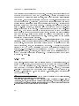
simplied level scheme of sodium in gure 2.10 where F denotes the total angular
momentum including the electron's and core's spin and the angular momentum of
the electrons. Each of the F states is now composed of 2F+1 degenerate magnetic
substates11 as shown in gure 2.10 for two energy levels.
Even though all this looks quite dierently from what has been discussed, the
cooling mechanism described above still works even better (see 2.2.4). The
laser is tuned slightly below the resonance F=2 to F'=3 and pairs of σ + and σ −
polarized12 counterpropagating beams are used. This drives the atoms to either
of the outermost substates shown in gure 2.10, depending on the direction the
atom is moving in and results in a Doppler cooling scheme.
Up to now, atoms may be cold, but trapping is not yet achieved since no
position dependent force is established. Inserting two magnetic coils in an antiHelmholtz conguration yields a magnetic quadrupole eld. The magnetic eld
introduces a position dependent Zeeman shift of the magnetic sublevels. The
resonance frequency of the cycling transition is shifted by
∆Zeeman =
1
gm0F − gmF µB B(~x) ≈ 1.4 MHz/G · B(~x)
~
(2.15)
For an introduction to selection rules and designation of levels in atoms refer to any standard
textbook like [50].
12
Often both of the beams are attributed the same polarization, however, this is a question of
the reference frame.
11
28
2.2 Magneto-Optical Trapping
Na D2-transition
32P3/2
F'=3
58.3MHz
15.8MHz
F'=2
mF'=-3 mF'=-2 mF'=-1 mF'=0
sF=2
mF'=-2
mF'=+1 mF'=+2 mF'=+3
s+
mF=-1
mF=0
15.8MHz
Repumper
F'=3
34.3MHz
589.756nm
508.332THz
F'=1
F'=0
Cycling Transition
23
F=2
2
mF=+1 mF=+2
3 S1/2
1.7716GHz
F=1
(a)
(b)
a) : Magnetic substates of the cycling transition used for sodium, b) :
Level scheme of sodium.
Figure 2.10:
where gmF and gm0F are the Landé factors of the involved states (see gure 2.11)
[64, 65]. This equation holds only for low magnetic elds as long as the nuclear spin
is mainly coupled to the spin-orbit momentum of the valence electron (compared
to the coupling to the external magnetic eld). We now have to modify equation
(2.14) a last time including equation 2.15. Now the scattering rate, nally, reads:
γscatter =
Γ
2
S
1+S+
2(∆+~k·~v +∆Zeeman )
Γ
2
A schematic of the line shifts is given in gure 2.11. Choosing the right magnetic
eld direction implies a force always directed to the magnetic zero.
In conclusion, there are two eects leading to magneto-optical trapping. Whenever an atom has got a certain velocity its absorption line is shifted into resonance
with a beam traveling in opposite direction. Whenever an atom is o the center
of the magnetic quadrupole eld the cycling transition is shifted into resonance
with a counterpropagating beam, leading to a backward force. This is visualized
in gure 2.11. The motion of atoms in a MOT is now characterized by a spring
constant attributed to the Zeeman shifting and a damping coecient arising from
the optical molasses. Since damping is much bigger than the spring constant, the
atomic motion is overdamped.
29
Frequency
Chapter 2 Theory
+
s -Light
+3
mF'=
mF'=
-3
w0
mF= -2
s--Light
wL
mF= +2
0
Magnetic field / Position
Trapping schematic in a MOT. σ + and σ − denote the polarization
of the light beams coming from the left and right respectively. ω0 denotes the
unshifted resonance frequency, ωL is the frequency of the laser beams that is
slightly detuned to the red. Read the x-axis to be the magnetic eld or in the case
of a MOT with B(x) ∝ x also as the position in a trap. For weak magnetic elds
the Zeeman substates are shifted such that ∆Zeeman = ~1 (gF 0 mF 0 −gF mF )µB B(~x),
with F 0 = 3, F = 2, mF 0 = ±3, mF = ±2, gF 0 = 0.6671 and gF = 0.5006 →
gF 0 mF 0 − gF mF = ±1.0002 ≈ ±1 [64]. An atom on the right will mainly absorb
photons from the σ − -beam and vice versa, pushing the atoms to the center.
Figure 2.11:
2.2.4 Sub-Doppler Cooling
The standing light wave, formed by two counter-propagating, circularly polarized
beams, is linearly polarized at each point. The polarization vector rotates along
the beam with a periodicity of half the wavelength. This inuences transition
amplitudes within the level scheme in such a way that an additional cooling mechanism arises leading to more ecient cooling, referred to as sub-Doppler cooling
[66, 67]. Temperatures on the order of 10µK can be achieved for sodium, corresponding to the kinetic energy associated with a single photon momentum recoil.
This is referred to as the recoil limit.
Already at that point it becomes clear that sub-Doppler cooling will not work
for lithium (see gure 3.4). The excited states are separated by less than the
30
2.2 Magneto-Optical Trapping
natural linewidth, thus, selective excitation of only one F state is not feasible.
2.2.5 Repumping
One point has not been mentioned yet. According to equation (2.14) electrons
in sodium may also be excited to the F'=2 state, since the level spacing is not
innite. Thus, transitions to the F=1 state are no longer dipole forbidden. Once
an atom is in the F=1 state it is no longer trapped and needs to be transferred
back to the F=2 state. Therefore, a repumping beam resonant with the F=1 to
F'=2 or F'=1 transition is added. This eect is even more pronounced in lithium
due to the quasi-degeneracy of the excited states. See 3.5.2 for more details.
2.2.6 Limitations and the Dark Spot MOT for Sodium
The density in a sodium MOT is limited to about 1011 cm−3 mainly by a process
called radiation trapping [68]. Already at much lower densities the atoms are
no longer interacting only with the light eld but they also reabsorb photons that
have been scattered by the others. These incoherent processes introduce a repulsive
force between the atoms and keep them apart.
This peak density can be increased by nearly a factor of ten if the atoms in the
center of the trap are in the untrapped F=1 ground state. This can be achieved
by removing the repumping light in the center of the trap ("dark spot")13 [69].
Without a repumping beam the atoms fall down to the dark F=1 state after about
100 scattering processes and radiation trapping is reduced. Repumping only occurs
at the edge of the MOT, keeping the atoms in the middle.
13
Originally SPOT is a short form for SPontaneous-force Optical Trap.
31
Chapter 2 Theory
32
3 Experimental Setup
The following chapter will give an overview of our setup with an emphasis on the
laser system. We use two optical tables of 3 m × 1.5 m each for the vacuum setup
on the one hand and for all the optics and light preparation on the other hand.
The two are interconnected using optical bers for the light and a BNC bus for
the exchange of data.
3.1 Introduction
In gure 3.1 we show an overview of our vacuum system that has been set up
during the last year. As it is characterized in more detail in Marc Repp's diploma
thesis we will only give a short summary on design guidelines and functionalities
in the following. The objective of our apparatus is to cool as many 6 Li atoms as
possible - on the order of 107 should be realistic [70] - to the lowest temperatures in
reasonably short time. Limiting factor for the number of fermions in the degenerate
phase is the number of sodium atoms initially trapped, since sympathetic cooling
results in huge losses of sodium atoms. The group of W. Ketterle reports on losses
of about 50% for lithium during the transfer to the magnetic trap and another
factor of two during the sympathetic cooling stage [71]. Thus, a lithium atom
number on the order of 108 in the MOT should be sucient.
These 107 6 Li -atoms need to be cooled at the expense of sodium. So cooling
will only be possible as long as suciently many sodium atoms are available.
Taking into account transfer eciencies from the MOT to the magnetic trap of
about 30% for sodium1 , less than 1% of the sodium atoms are left after evaporative
cooling, where this number highly depends on the starting and nal temperature
as well as the atom number in the fermionic cloud. As a rule of thumb sympathetic
cooling is ecient as long as there is at least a comparable number of sodium in
Up to ≈70% can be achieved with more elaborate transfer mechanisms to the |F', mF' i =
|1, −1i state [48]. However, these are not applicable in our case. See discussion in [71] and in
section 3.4.2.
1
33
Chapter 3 Experimental Setup
the magnetic trap [71]. Thus, an initial 1010 sodium atoms should be captured in
the MOT.
3.2 Vacuum System
For this experiment a vacuum apparatus with a residual pressure well below
10−10 mbar is needed. This is for several reasons. The mean free path of the
atoms needs to be much larger than the length of the apparatus, such that the
atoms in the atomic beam are not deected on their way from the oven to the
glass cell (see next section). However, the stronger constraint is, that during an
experiment, i.e. on the order of a minute, cold atoms should not collide with hot
atoms.
3.2.1 The Vacuum Chamber
A possible way to high loading rates using sodium and lithium is a linear setup
with ovens, a Zeeman slower and a glass cell.
(6)
(9)
(7)
(8)
(12)
(10)
(3) (4)
(11)
(1) (2)
(15)
(5) (13)
Figure 3.1:
(14)
Overview of our vacuum apparatus, see text for more details.
In the following the numbering relates to gure 3.1. Our setup consists of an
arrangement of two ovens for sodium (1) and lithium (2), heated up to 270 ◦ C
and 350 ◦ C respectively. They are connected through an angled mixing nozzle (3)
that allows liquid sodium to ow back into the reservoir. These temperatures are
needed in order to increase the (very low) vapor pressures for these two elements
(cf. [64, 65]). Sodium and lithium vapors are brought together in the lithium
part of the oven and nally diuse into the apparatus through a conical hole with
inner diameter of 4 mm (referred to as "oven nozzle") (4). Pressures and, thus,
the ratio of emitted atoms into the ultra high vacuum chamber and the total ux
34
3.3 Zeeman Slower
can be adjusted by selecting the temperatures in the two oven chambers. About
10 cm behind the oven nozzle there is a rotary feedthrough (5) inserted into our
vacuum system. This feedthrough is connected to a thin plate made of stainless
steel serving as a shutter for the atomic beam. During this diploma thesis a driver
has been developed, that allows to switch the atomic beam on and o with TTL
signals. Basically this driver uses a standard RC-servo and is controlled by a small
PIC microcontroller. See appendix B for more details.
A small aperture at position (6) is blocking atoms on o-axis trajectories. The
transmitted atomic beam is sent through two dierential pumping tubes ((7) and
(8)) permitting to decrease the residual gas pressure gradually from 5 · 10−8 mbar
to 10−11 mbar. We will present the Zeeman slower (9) in the next section. The
Zeeman slower is put as close as possible to the glass cell avoiding too many losses
due to the elevated divergence of the beam at that point. The glass cell (10) itself
is attached to exible bellow adapters via a glass to metal transition2 . Behind the
glass cell, there is a vacuum gauge (11) and a window for the Zeeman slower beam
(12).
3.2.2 Pumping
Our vacuum setup is evacuated by two 55 l/s ion getter pumps (one (13) in the
oven and collimation section, the other one (14) in between the two dierential
pumping tubes) and a 150 l/s ion getter pump (15) combined with a titanium
sublimation pump (about 1000 l/s) behind the glass cell.
For a more detailed description of our setup and an analysis of vacuum conductivities and pumping speeds refer to Marc Repp's diploma thesis [72].
3.3 Zeeman Slower
A Zeeman slower has been installed in order to increase the ux of slow capturable
atoms in the glass cell. Loading of a magneto-optical trap requires slow atoms with
speeds of less than 30 m/s as a rough estimate, whereas the velocity distribution
of sodium and lithium atoms is centered around 800 m/s and 1600 m/s for the
given oven temperatures. Evidently, only a very small fraction is captured without
further precautions. In the Zeeman slower atoms can be decelerated to the required
speed. Our slower is designed such that sodium and lithium atoms with initial
When heating up the vacuum the dierent specic expansion coecients of steel and glass
would in either case make the cell burst. So the expansion coecient needs to be changed
gradually.
2
35
Chapter 3 Experimental Setup
speeds of up to 700 m/s can be slowed down. The most probable velocity of the
atoms leaving the oven is about the same for sodium, but about twice as high
for lithium. Thus, the ratio of slowed sodium atoms is much bigger than that of
lithium. Since more sodium than lithium is needed for the further cooling, this is
not a restricting point.
Below I will briey describe the functional principle of a Zeeman slower and
some design criteria of the one we set up. For more details on any point refer to
Jan Krieger's diploma thesis [73].
3.3.1 Design Criteria
• Our slower was designed for sodium. As discussed before, more sodium than
lithium is needed for further cooling steps. A sodium slower always works
for lithium but is more conservative .
3
• The slower should be considerably shorter than 1 m, rst for keeping the
apparatus compact, but also since the (geometric) divergence of the atomic
beam cancels the slowing eect at some point. Random scattering of the
absorbed photons leads to additional transversal heating, i.e. divergence.
• In order to compensate for imperfections of the magnetic eld the design
used a saturation parameter S equal to one, even though more laser power
is available.
• The magnetic eld should not be excessively high close to the center of the
MOT coils, since it has to vanish there. In addition, the Zeeman slower beam
should not be resonant to the atoms in the MOT. This condition requires a
non-zero eld at the end of the slower.
3.3.2 The Setup and a Basic Introduction
Our Zeeman slower consists of two solenoids with an overall length of about 70 cm
with an additional free space of about 20 cm between them. The solenoids are
concentric to the atomic beam. Along this axis a laser beam and the atomic beam
counterpropagate. Whenever the circularly polarized laser beam is resonant with
an electronic transition light is absorbed and scattered into any direction, leading
to a mean deceleration. Shaping the magnetic eld B(z) such that deceleration
(i.e. Doppler shift of the atomic lines) is compensated by Zeeman shifts of the used
A slower designed for lithium only would have been shorter while maintaining the same
slowed fraction of slowed atoms.
3
36
3.3 Zeeman Slower
transitions the atoms are resonant all along the magnetic eld and, thus, slowed
down.
Atoms moving at velocity v in a position dependent magnetic eld B(z) with
a counterpropagating laser beam with wavenumber k experience a deceleration
a(z, v) =
~k Γ
m2
1+S+
S
2δ(z,v)
Γ
2
µB gB(z)
δ(z, v) = δ0 + ~k · ~v −
~
(3.1)
(3.2)
where ~ denotes the reduced Planck constant, Γ is the line width of the transition of the excited atoms, the Landé factor g for the used transition is very close to
one [64, 65], m is the atomic mass and S is the saturation parameter (refer to [59]
for more details on atom light interaction). δ0 is called laser detuning and is given
by the dierence between the laser and the atomic resonance frequency. Elimination of v while keeping a constant for all z implies a square-root shaped magnetic
eld. Main characteristics of a Zeeman slower are the S parameter needed for
slowing (in our case S should be on the order of 1), the maximal velocity that can
be slowed (in our case about 700 m/s for both species) and the conguration of
the magnetic elds. We set up a slower in a so-called zero crossing conguration
(also known as "spin-ip slower" [74]). "Increasing eld" and "decreasing eld"
slowers do not need a zero-crossing. However, they have their maximal magnetic
eld close to the MOT or zero eld close to the MOT, i.e. Zeeman slower light is
resonant with the atoms in the MOT.
This means that the magnetic eld starts at about 600 G and decreases down to
−200 G. In the zero eld domain atoms have to repolarize because of the change in
magnetic eld direction leading to a change from σ + to σ − light in the rest frame of
the atoms. The advantage of such a conguration is that the magnetic eld close
to the magneto-optical trap is relatively small (about 200 G). So compensation
of the magnetic eld can be achieved with little eort. This is necessary, since
the magneto-optical and magnetic trap would be perturbed. On the other hand,
the Zeeman laser beam is still far detuned relative to the unshifted resonance and
MOT operation is not disturbed by this light. The only disadvantage is that one
needs repumping light since during the repolarization at zero eld any magnetic
substate of the excited state is populated. So decays to the ground state 32 S1/2 ,
F=1 may occur, and atoms in that "dark state" would be lost for further slowing.
Another point is that sucient time for this repolarization process needs to be
provided resulting in a longer slower.
37
Chapter 3 Experimental Setup
3.4 Magnetic Fields
For magneto-optical trapping, magnetic trapping and tuning of scattering lengths
in the vicinity of Feshbach resonances only one single pair of coils are used, creating
a quadrupole eld in an anti-Helmholtz conguration or a homogeneous eld at
the center for a Helmholtz conguration, depending on the relative polarity of the
coils. Here the Feshbach coils are the challenging part. They will be described in
the following.
Drawing of our multi functional coils used for magneto-optical and
magnetic trapping as well as for Feshbach elds
Figure 3.2:
3.4.1 Feshbach Coils
Tuning over atomic Feshbach resonances of a degenerate Fermi gas opens up a wide
eld of exciting physics that becomes accessible as described in the introduction
(see chapter 1.2). In a standard experiment interaction is tuned to some scattering
length in the range of the Feshbach resonance, i.e. a magnetic eld of about 830 G
for 6 Li . Typically, the interaction needs to be switched very quickly. Our coils are
designed such that they can be switched from 1000 G to zero in less than 20 µs. For
a minimal switching time and bearable inductive voltages the inductance needs to
be kept as low as possible. So in order to reach the high magnetic elds huge
currents (up to 440 A in our case) have to be put through the wire leading to
dissipated powers on the order of 2 kW. Heat management is an important point
since any temperature instability causes uctuations of the magnetic eld gradient.
38
3.4 Magnetic Fields
In this kind of experiment one relies on reproducible results on a timescale of hours,
thus, any heating eects have to be minimized. The assembly that is currently set
up consists of four coils of the type shown in gure 3.2, two above and two below
the glass cell with 15 windings each. Hollow squared wire has been used such that
the heat can be removed by temperature-regulated water owing through. The
assembly is embedded in epoxy.
3.4.2 Magnetic Trap
For magnetic trapping we will use a quadrupole magnetic eld. Therefore, the
multi function coils are switched to an anti-Helmholtz conguration by means of a
bridge circuit based on insulated-gate bipolar transistors (IGBT4 ) (for more details
refer to the diploma thesis of Anton Piccardo-Selg [75]). The magnetic eld is zero
in the center of the assembly and increases linearly in radial and axial direction
(with a gradient that is twice the value for the radial direction). For magnetic
trapping the atoms need to be transferred to some low-eld seeking state that is
immune towards spin-exchange collisions5 . These atoms will now oscillate around
the zero.
There are only two states for sodium with a non-vanishing magnetic moment
satisfying these conditions, namely |F, mF i = |1, −1i and |2, 2i. The |1, −1i
state is preferred6 by far for creating sodium BECs, yet it undergoes spin exchange
collisions with lithium (see discussion in [71, 48]). So the |2, 2i state is the one
to choose. Optical pumping in a small magnetical bias eld allows to transfer the
atoms to the |2, 2i state (see section 3.5.2.7).
Once in the center there is no longer a polarizing eld, spin ips occur and
atoms (in untrapped states) are lost. In order to avoid this, several trap congurations have been developed such as clover-leaf [77], Ioe-Pritchard [78] or
time-orbiting potential (TOP) [79] traps. We use a standard quadrupole magnetic
eld combined with a blue detuned laser beam7 focused into the center of the trap
("optical plug", [80]). The light shift potential8 induced by this beam keeps the
trapped atoms away from the magnetic zero.
Transistors designed for switching of high currents, i.e. several hundreds of Ampères.
Collisions that change the internal spin state of the atoms, transferring them from a trapped
to an untrapped state
6
Not only the |2, 2i state, but also the |2, 1i and |2, 0i are (at least weakly) trappable in a
the magnetic trap. Since there are spin exchange collisions between them, the latter need to be
completely removed in order to close this loss channel [71, 48, 76].
7
We will use some of the pump laser power at 515 nm.
8
Potential attributed to the optical dipole force of the light (see 2.2.1.1).
4
5
39
Chapter 3 Experimental Setup
3.5 The Laser System
As described in section 2.1.3 our laser system is based on two Radiant Dyes Ring
Dye Lasers. They are pumped by a frequency doubled Yb:YAG disc laser with
two outputs at >10 W each. For sodium we are using a dye solution of rhodamine
6G in ethylene glycol. The concentration is set such that the pump laser beam
is absorbed to about 98% within the dye jet yielding concentrations of about
0.8 g/l. The maximal power exceeds 1 W for 8 W of pumping power. However,
stable, mode-hop free operation is currently only possible at about 800 mW. This
is probably due to heating of the dye in the center of the pumping spot. With a
higher dye jet speed higher stable powers should be easily achievable. Therefore,
either more powerful dye circulators, or a thicker dye nozzle are needed. The dye
used for Lithium light is DCM with a concentration of about 0.8 g/l in a mixture of
50% ethylene glycol, 18% benzyl alcohol and 32% propylene carbonate. Its power
exceeds 1.5 W. Stability tests have not yet been performed.
3.5.1 Why Dye Lasers?
Because there is currently no well-developed alternative for sodium light at 589nm.
At the Laboratoire Kastler-Brossel (ENS) Fabrice Gerbier et al. are currently
developing a solid state laser at 589 nm using frequency mixing of diode lasers.
However, power output is below 400 mW up to now. Already available commercially are small Diode Pumped Solid State (DPSS) modules with a second harmonic
generator but they are far away from single mode.
In the case of lithium there are actually cheap laser diodes with powers of up
to 100 mW available (e.g. laser diode type HL6545MG9 ) that are used in DVD
recorders. Another alternative would have been Toptica's TA modules (based on
tapered ampliers) oering up to 500 mW. But even though dye lasers are more
demanding than solid state lasers they oer a mode quality that is far better than
laser diodes. Additionally the output power is suciently high.
3.5.2 Frequencies
All frequencies had to be derived from one single laser using acousto-optical (AOM)
and electro-optical (EOM) modulators. Consequently, the design of the laser system has to comply with some basic requirements:
These diodes have rated powers of up to 120 mW. However, their typical wavelength is
662 nm and they need to be heated up to about 65◦ C for 671 nm.
9
40
3.5 The Laser System
6
F'=3
Li D2-transition
F'=5/2
F'=3/2
58.3MHz
15.8MHz
F'=2
15.8MHz
Repumper
589.756nm
508.332THz
F'=1
F'=0
34.3MHz
2
3 P3/2
4.4MHz
F'=1/2
Repumper
3 P3/2
670.977nm
446.800THz
2
Cycling Transition
Na D2-transition
Cycling Transition
23
F=2
F=3/2
32S1/2
2
3 S1/2
1.7716GHz
76MHz
228MHz
F=1
Figure 3.3:
F=1/2
Level scheme of Na
23
Figure 3.4:
Level scheme of Li
6
• ecient use of laser power
• maximal tunability of frequencies
• cost eective use of standard optics (thus, especially use of standard AOMs)
Figures 3.3 and 3.4 show the level schemes of the relevant transitions in 23 Na and
6
Li. For simplicity the D1 -lines have been omitted. They are about 400 GHz and
10 GHz below the corresponding D2 -lines for sodium and lithium and, thus, not
interfering with any process discussed in the following.
In the following we will give an overview of the frequencies needed. The lithium
laser system has not been set up until now, so only a proposed scheme is given in
gure 3.9 and table 3.1.
3.5.2.1
Locking the Laser to an Atomic Resonance
Both lasers are locked internally to a temperature stabilized reference cavity with
a short term stability of about 1MHz. However, on the timescale of hours (or even
seconds) a stability well below the natural linewidth of lithium (ΓLi = 2π · 6 MHz)
and sodium (ΓN a = 2π · 10 MHz) can not be guaranteed10 . Long-term stability is
provided by locking the laser to an atomic transition. At room temperature, a cell
lled with some 23 Na or 6 Li is not sucient to show appreciable absorption due to
The time constant of the feedback loop is limited by the mechanical (!) galvo plate within
the reference cavity, thus, on the order of hundredths of seconds.
10
41
Chapter 3 Experimental Setup
the minuscule vapor pressure of both species. Therefore, absorption cells have to
be heated up to about 130◦ C and 240◦ C, respectively. A sodium spectroscopy oven
has been set up during this diploma thesis, based on an evacuated glass cell lled
with sodium. More technical details on this and on Doppler-free spectroscopy can
be found in appendix D. For lithium, a somewhat more elaborate scheme is needed
because lithium diuses into glass and chemically reacts with it. This leads to an
increased opacity and permanent damage. Typically, this problem is overcome
using a so-called heatpipe, a relatively long and thin tube made of high-grade
steel, that is heated in the middle. The inner surface is covered with a high-grade
steel mesh. The windows attached on either side are kept at room temperature
and a small amount of buer gas is brought into it, avoiding any direct collisions
with the windows. Lithium atoms hitting the walls o the center stick to them
and diuse back to the center along the mesh. See [16, 81] for a more detailed
analysis and concrete implementations.
The sodium laser is locked to a frequency of -180MHz11 relative to the cycling
transition, mainly because this simplies the whole optics scheme. Another point
about this is, that any stray light is far detuned (about 8Γ) relative to the next
atomic resonances, thus, not interfering at any point. The laser is not locked
directly to the F=2 to F'=3 transition but to the most signicant feature of the
spectrum, i.e. the cross-over of the transitions F=2 to F'=3 / F'=2, that is about
-29MHz red detuned. Therefore, one needs to shift up the laser's frequency by
about
before doing spectroscopy. A measured spectrum can be found
in gures D.5 and D.6.
+151MHz
3.5.2.2
MOT
For magneto-optical trapping light is usually detuned by several linewidths. For
sodium atoms, however, a red detuned beam is at the same time blue detuned for
the F=2 to F'=2 transition and, thus, pushes out the atoms. This inuence can
only be reduced by choosing a relatively small detuning. Up to now, we are using
-15MHz (
) as a compromise of the values used in the groups of W.
Ketterle (∼-20MHz) and P. van der Straten (∼-11MHz), since no systematics
have been done yet12 .
+165MHz
any bold frequencies given are from here on meant to be relative to the cycling transition,
bold italic frequencies relative to the laser frequency
11
12
One might think of choosing a MOT frequency below the lowest hyper-ne state at
<110MHz, however, in this case only Doppler cooling will occur. At the same time, repumping
power needs to be increased drastically since transitions to the F=1 state are no longer forbidden
an inconvenient point as will be seen in the next section
42
3.5 The Laser System
23
δ
MHz
MOT
−15
MOT repumper
+1679
Zeeman slower
−350
Zeeman slower repumper +1713
Imaging
0
Transfer
−58
Lock Frequency
−180
Na
δ
MHz
+165
+1859
−170
o
+180
+122
0
rel
13
6
Intensity
> Isat
4 mW
IZ Isat
≈ 10% · IZ
< 1 mW
≈ Isat
0.5 mW
δ
MHz
−25
+228
−344
−116
0
o
−182
Li
δ
MHz
+157
+410
−162
+66
+182
rel
14
0
Frequencies needed, where δ is the detuning relative to the atomic
resonance and δrel is the detuning relative to the laser frequency.
Table 3.1:
3.5.2.3
MOT Repumper
A priori the cycling transition in sodium is closed, where closed means, that decays
into the "wrong" F=1 ground state are dipole forbidden. Since the hyper-ne
splitting of the excited state is small compared to the linewidth, excitations to the
F'=2 state actually may occur. Electrons may now decay into the F=1 state and
are no longer trapped. Putting a repumping beam resonant with the F=1 to F'=1
(+1679 ) transition returns atoms into the cycle. Taking the relevant
Clebsch-Gordan coecients into account the F=1 to F'=2 transition would have
been favorable. The advantage of our selected resonance is that, given a repumping
beam that counterpropagates the Zeeman slowed atomic beam under an angle of
about 50◦ , the atoms experience shifted light, that is resonant with the F=1 to
F'=2 transition. In conclusion the F=1 to F'=1 transition is used for repumping
of trapped atoms, the F=1 to F'=2 transition for the incident beam that is about
to be trapped. Yet the eect of this method still has to be evaluated.
+1859
3.5.2.4
Zeeman Slower
The magnetic end eld and the desired speed of the atoms dene the detuning
for the Zeeman slowing beam. We arbitrarily chose the magnetic eld maximum
close to the glass cell to be 214 G with a speed of the atoms of vend = 30 m/s, corresponding to the capture velocity of the MOT. The contribution for the relevant
Zeeman shift and Doppler shift reads now:
13
14
Sidebands are directly modulated onto the Zeeman slower beam.
Hyper-ne levels of excited state are not resolved.
43
Chapter 3 Experimental Setup
∆Zeeman, end = −µB Bend = −1.4MHz/G · 214G = 300MHz
∆Doppler, end = −vend /λ = −50 MHz
(3.3)
(3.4)
where µB denotes Bohr's magneton. This total detuning of -350MHz corresponds
to
relative to the laser frequency.
-170MHz
3.5.2.5
Zeeman Slower Repumper
In regions of strong magnetic elds within the Zeeman slower, the distance between the cycling transition levels and the other energy levels is increased such
that the loss process described in the penultimate section is strongly suppressed.
Repumping is only necessary in the domain of the zero crossing of the magnetic
eld. In the rest frame of the atoms a change of the magnetic eld changes the
character of the light from σ + to σ − and vice versa, thus, pumping from one outermost magnetic substate (mF 0 = 3) to the other (mF 0 = −3) is accomplished.
During this repolarization process decays into the F=1 ground state are no longer
forbidden. Consequently, it is here that the repumper has to act. The repumper
needs to be detuned by +1713 MHz minus the Doppler shift at the point of the
zero crossing. However, since it is directly modulated onto the Zeeman slowing
beam as described in section 3.5.3 this Doppler shift drops out16 .
3.5.2.6
Imaging
When doing experiments with cold atoms most of the information on the system
is derived from images. To take a picture ("absorption image") the atomic cloud
is illuminated briey with a weak collimated beam of resonant light (+0MHz,
) and scatters photons proportional to its local particle density. This
produces a shadow of the cloud that is recorded by a camera.
+180MHz
3.5.2.7
Transfer into a Magnetic Trap
As briey discussed in section 3.4.2 the atoms need to be transferred to the loweld seeking |2, 2i state before being transferred to the magnetic trap. Ecient
transfer can be achieved by shining in σ + -polarized light resonant to the F=2 to
F'=2 transition after switching o the MOT. This transfers the atoms to the dark
The Zeeman slower beam is - according to its working principle - on resonance all along the
magnetic eld, thus, especially at the zero eld. Consequently, a repumping beam shifted by
+1720MHz is resonant at that point, too.
16
44
3.5 The Laser System
|F', m i = |2, 2i state, without any further heating. Therefore, light at -58MHz
(
) is needed.
+122MHz
F'
Fabry-Perot
Transmission [arbitrary units]
3.5
3
FSR=1.5 GHz
2.5
2
1.5
1
220 MHz
0.5
0
-2. -1.
-0.5
400
600
800
1000
0. +1. +2.
1200
1400
1600
1800
2000
2200
Time [arbitrary units]
Transmission through a scanning Fabry-Perot interferometer with free
spectral range (FSR) of 1500 MHz of a beam behind an EOM driven at 1720 MHz.
Since the FSR is inferior to the mode spacing, the signal of the n-th sideband is
folded back by a multiple of the FSR and appears at n times 220 MHz from the
peak. The incoupled RF power was about 2.5 W.
Figure 3.5:
3.5.3 Frequency Generation
All but two frequencies are shifted using acousto-optical modulators (AOM) fabricated by Crystal Technology Inc. These contain a radio frequency (RF) transducer
attached to a transparent crystal of tellurium dioxide. Driving the transducer with
RF powers of typically 0.5 W creates a running sound wave inside the crystal. Photons crossing the TeO2 crystal will experience Raman processes, i.e. absorb or emit
a phonon if the angle of incidence is such that quasi-momenta and energy is conserved. The photon's frequency can change in that way by integer multiples of
the RF, where only the rst orders are used in our experiment. Passing the light
twice through one single AOM by retroreecting results in a shift of twice the RF.
Commercial standard AOMs are available typically at frequencies of 80, 110 and
200 MHz with bandwidths of about 10%. Our optics schemes have consequently
been designed such that all high power beams are shifted by AOMs close to resonance, in order to achieve highest possible eciencies. The AOMs used in a
double-pass conguration have been set up similar to the proposition in [82].
Two exceptions concern the repumping light. For the MOT repumper we use
an AOM at about 1.9 GHz provided by Brimrose Corporation of America (see
gure 3.6). This device is far o from being standard and to our knowledge 45
Chapter 3 Experimental Setup
can only be fabricated by the aforementioned company. Nominal eciency is as
high as 15%, however, the outcoupling aperture is too small. Since we need to
recycle the zeroth order only 5% can be achieved without clipping at the housing.
This is still sucient for our purposes. For the Zeeman slower repumping light an
electro-optical modulator (New Focus Inc.) with a center frequency of 1720 MHz
is used. An incoupled RF-eld is reinforced resonantly inducing a eld dependent
optical path by means of the Pockels eect. This sine shaped modulation creates
sidebands to a laser beam passing through at ±nf , where n is an integer and f
is the radio frequency17 . In gure 3.5 there is an example for what the spectrum
looks like behind the EOM.
The drivers for these high frequency modulators have been assembled during
this thesis and are briey described in chapter E.
(a)
(b)
a) : Acousto-optic modulator at 1.9 GHz. The housing has been manufactured in order to keep dust apart. b) : MOT beam assembly.
Figure 3.6:
2
The Power within the n-th sideband is proportional to |Jn (φ)| , where φ is proportional to
the square-root of the RF-Power and Jn (φ) denotes the n-th Bessel function.
17
46
3.5 The Laser System
3.5.4 The MOT setup
As mentioned in section 2.2, a MOT requires three pairs of beams with opposite
circular polarizations18 and a quadrupole eld. The multi functional coils described
in section 3.4 are also used for the magneto-optical trap. On the optical table the
MOT light is coupled into a single-mode polarization maintaining ber that is
split into three pairs of bers by a micro-optics device manufactured by Canadian
Instruments19 . While the power in two bers of one pair is very close to equal
(±2%), dierent pairs vary by up to 10%.
This ber splitting unit greatly reduces the optics for the MOT - we only
need to collimate the light and choose the right polarization. Therefore, a mount
holding ber holder, λ/4-plate and a 100 mm lens has been built (see gure 3.6).
250
200
150
100
50
Figure 3.7:
3.5.4.1
Dark spot
Repumping Light for Sodium and the Dark Spot MOT
The repumping light is coupled into a multimode ber, mainly because the high
frequency AOM destroys the Gaussian mode needed for ecient ber coupling
and no puried Gaussian mode is needed for repumping. In a further step, we will
implement a so called dark spot MOT. As described in section 2.2.6 the number of
Actually there are geometries requiring only four beams [83], however, achieving big stable
MOTs like this is dicult.
19
Actually a more power saving strategy is to retroreect the MOT beams and to change the
polarization using a λ/4-plate in front of the mirror. However, in an optically dense MOT the
returning beam is attenuated and balancing might be a problem. In spite of this the group of
van der Straten realized the biggest sodium MOT ever in this conguration [48].
18
47
Chapter 3 Experimental Setup
atoms can be increased by a factor of ten by blocking the repumping light in the
center of the MOT. By chance we found out that we can create a close to perfect
ring-shaped mode by sloppily coupling into the multi-mode ber. Focusing the
laser beam into the incoupler (instead of collimating the beam) obviously excites
whispering gallery type mode within the ber cladding. The width of the ring
structure can easily be tuned by displacing the focus relative to the incoupler.
The incoupling exceeded 50% without any further optimization. If ever the core
of the mode is not dark enough an additional aperture can be inserted without
losing much power. The outcoupled structure is shown in gure 3.7. The ring is
covered with a speckle pattern, even though we do not think that this will interfere
one could remove it by "shaking" the ber. The slightest movement of the ber
rotates the pattern, thus, a small loud speaker should suce20 .
20
48
Spatial ltering is an alternative, but breaks a buttery on a wheel!
3.5 The Laser System
MOT beam,
to fiber splitter
MOT To Zeeman
Repumper slower
Imaging
l/4
l/2
EOM
DYE LASER
AOM
80MHz
AOM
80MHz
+1
AOM
80MHz
l/2 1720MHz
AOM
1900MHz
l/2
l/4
l/2
l/2
+1
l/4
l/2
-1
RF-coils
+1
l/4
l/4
+1
Lock-In
Amplifier
PI-Loop
Sodium
Spectroscopy
AOM
80MHz
l/4
Polarizing
Beamsplitter
Cube
Window
Beam
Dump
Lens for
"Cat's Eye"
Fiber
Coupler
PhotoDiode
Mirror
Overview of our sodium laser setup, the transfer beam for the magnetic
trap has not yet been implemented.
Figure 3.8:
MOT
to fiber splitter
Zeeman
Slower
l/2
MOT
Repumper
l/2
l/2
l/2
l/2
l/2
l/2
AOM
80MHz
l/2
Imaging
DYE LASER
AOM
80MHz
AOM
80MHz
-1
+1
l/4
l/4
+1
l/4
AOM
80MHz
+1
l/4
l/4
l/2
PI-Loop
AOM
200MHz
+1
Zeeman
Slower
Repumper
Lock-In
Amplifier
AOM
150MHz
+1
Lithium
Heatpipe
l/4
Figure 3.9:
Draft of our lithium laser setup.
49
Chapter 3 Experimental Setup
50
4 First Measurements
This chapter will give the rst absorption measurements we have performed on
our magneto-optical trap for sodium. More extensive studies are part of Marc
Repp's diploma thesis [72]. Here we present the rst absorption measurements on
our MOT. All results we obtained have to be considered preliminary since this
work has still been done using some provisional coils. In addition, systematic
optimization of the dierent laser detunings, intensities and magnetic elds have
not yet been done. One change compared to Marc Repp's diploma thesis is that
the 1-on-6 ber-splitter has been installed in the meantime. However the number
of trapped atoms was still up to a factor of ten lower than before.
4.1 A Provisional Absorption Imaging System
4.1.1 Optical Density of an Atomic Cloud and the BeerLambert Law
Light crossing a sample of particles of density n is attenuated due to scattering
processes according to the Beer-Lambert law, if the scattering cross section σ is
independent of the light intensity:
(4.1)
It = I0 exp−σnd
where I0 and It denote the incident and transmitted intensity respectively and d
is the thickness of the sample.
The scattering cross section for atoms in a light eld is given by [48]:
σ=
σ0
1+S+
~ωΓ
where: σ0 =
2Isat
2δ 2
Γ
(4.2)
(4.3)
51
Chapter 4 First Measurements
Here δ is the detuning of the light, Γ is the linewidth (Γ = 2π · 9.98 MHz for
D2 -line of sodium), and S = I/Isat is the saturation parameter with the light
intensity I and the saturation intensity Isat for the given transition. σ0 is called
on-resonance cross section.
For atoms, the Beer-Lambert equation holds if:
1
!
≈1
2δ 2
1+S+
(4.4)
Γ
Thus if the light intensity is small compared to the saturation intensity. Beyond,
the scattering cross section decreases as a function of I . For resonant light of low
intensity only σ0 has to be known.
The optical density being dened as
OD = ln I0 /It
(4.5)
can now be related to the particle density using equations (4.5) and (4.1):
n=
OD
σd
(4.6)
Given an absorption image (thus the optical density as a function of two spatial
directions x and y , z being the direction of the imaging beam) the total particle
number N can be calculated using:
Z
+∞
Z
+∞
N=
−∞
−∞
OD
dx dy
σ
(4.7)
where the z direction ("d") just drops out since this integration has already been
done implicitely when projecting the cloud onto the camera.
On a discrete grid, dened by the CCD pixels, the integral turns into a sum:
N=
X OD
·A
σ
n ,n
x
(4.8)
y
where nx , ny denote the pixels of the whole image and A is the area of one pixel1 .
This equation remains valid if there is some optical magnication, since the scattered light
stays the same.
1
52
4.1 A Provisional Absorption Imaging System
4.1.2 A Provisional Imaging System
A provisional absorption imaging system has been set up using a "PCO pixely
vga" digital CCD camera system with a resolution of 12 bit. The dimension of one
pixel is 9.9 × 9.9 µm2 . An imaging beam resonant to the atomic transition with
very low intensity (≈ 10 µW/cm2 ) compared to the saturation intensity has been
installed. It passes through a single mode polarization maintaining ber and is
collimated on the vacuum table. Its angle of incidence onto the glass cell is about
20◦ . This reduces interference fringes due to multiple reections within the glass
cell.
0
optical density: 0.45
vertical position [mm]
1
0.4
0.35
2
0.3
0.25
3
0.2
0.15
4
0.1
5
0.05
0
6
-0.05
0
0.5
1
1.5
2
2.5
3
3.5
4
4.5
horizontal position [mm]
Figure 4.1:
Optical density of the magneto-optical trap.
For a quantitative analysis of the atom number, three images with atomic
cloud, without atomic cloud and without imaging beam have to be taken. The
latter ("dark image") is subtracted from the others in order to compensate for any
stray light and camera noise. The logarithm of the (point-by-point) ratio of the
resulting two images gives the optical density per pixel.
53
Chapter 4 First Measurements
4.2 Estimating the Atom Number in the Sodium
MOT
The diameter of the MOT we have analyzed was on the order of 2 mm. The
magnetic eld gradient of the quadrupole eld was below 10 G/cm, thus Zeeman
shifts of the atoms are on the order of 2 MHz and thus negligible. Doppler eect
(well below 1 MHz) does not play a role, either. Images have been taken with
the magnetic quadrupole eld still on2 . For an estimate of the atom number any
absorption properties depending on the quantization axis have not been taken
into account in the following and the minimal saturation intensity has been used
for calculations (for sodium: Isat = 6.2 mW/cm2 for the transition |F, mF i →
|F 0 , m0F i = |2, ±2i → |3, ±3i). Hence, the absorption image can directly be
identied as the density distribution projected onto the CCD. At the same time,
the number of particles is underestimated systematically.
0.4
Optical Density
Optical Density
0.4
0.3
0.2
0.1
0.3
0.2
0.1
0
0
0
1
2
3
4
Vertical Position [µm]
(a)
0
1
2
3
4
5
6
Vertical Position [µm]
(b)
Averaged column density prole (a) and row density prole (b) ) shown
in gure 4.1 together with Gaussian ts.
Figure 4.2:
Figure 4.1 shows one of the rst images taken, in gure 4.2 the averaged row
and column density proles are shown. Evidently, the optical density is low. Using
equation (4.8) yields an atom number on the order of 2 · 107 . A Gaussian plot to
the line proles yields diameters (FWHM) of da = 1.20(2) mm in vertical (axial)
and dr = 1.92(2) mm in horizontal (radial) direction. Evidently, the cloud has
not a Gaussian shape in horizontal direction but the row prole is slightly tilted.
2
54
Our interim coils could not be switched fast enough.
4.2 Estimating the Atom Number in the Sodium MOT
This may arise as soon as the eective potential of light and magnetic forces is
no longer harmonic but contains higher order terms. Probably the Zeeman slower
beam contained some close to resonant stray light pushing the magneto-optical
trap slightly.
Assuming the cloud to have the same thickness in both radial directions the
peak density in the center is given by:
√
8( ln 2)3 N
nmax =
≈ 109 atoms/cm3
(4.9)
3/2
2
2
π dr da
The low optical density indicates that multiple scattering processes do not yet play
a dominant role. In this case atoms move in a quasi-harmonic potential [72, 84]
and one would expect a Gaussian density distribution. This justies the Gaussian
t in gure 4.2.
Refer to Marc Repp's [72] diploma thesis for loading and loss rates as well as
temperature estimates.
55
Chapter 4 First Measurements
56
5 Résumé and Outlook
5.1 Current Progress of the Experiment
One year ago, we started to set up an experiment on degenerate Fermi gases of
6
Li with bosonic 23 Na as a refrigerant. During this year, we have installed a laser
system for cooling and trapping of 23 Na and a vacuum apparatus. Also a new lab
has been equipped from zero (see page (iii)) . A rst magneto-optical trap for
sodium atoms with on the order of 108 atoms has been seen, however these results
have to be considered as preliminary.
In the meantime the nal coils together with working oset coils (for compensation of any stray magnetic elds) have been installed and the vacuum apparatus
(formerly slightly bent), has been straightened. Furthermore, a running version
of the computer control has just been released. Altogether, this should allow for
increasing the number of trapped atoms drastically. Especially since from now on
systematic optimization will be greatly simplied.
5.2 Outlook
An important milestone on our way to degeneracy will be the rst BEC of sodium.
Before there are still some steps to take. First of all our multi function coils,
installed since end of October 2007, need to be put into operation. Afterwards
the rst thing to do will be to increase the atom number within the magnetooptical trap using a dark spot technique and the transfer into the magnetic trap.
Another ongoing project is the design and construction of the microwave antenna
for 1.8 GHz and drivers that will be used for RF evaporative cooling.
Once the BEC has been obtained the lithium part will be tackled. For this
purpose, the lithium laser system still needs to be set up. Yet the optics needed
57
Chapter 5 Résumé and Outlook
is already available and this part should not take too much time. In parallel, a
proper imaging system needs to be set up. Probably similar to the one installed
in our rubidium BEC experiment next door [85]. A nal thing is the transfer of
the species to an optical dipole trap and this is where the actual experiment will
begin...
58
A Sodium Data
A simplied level scheme of sodium can be found in gure 3.3. The vapor pressure
is plotted in gure D.2.
Table A.1 nally lists some important optical properties of sodium. For further
information refer to [64].
Frequency without Hyperne-Shift
Transition Energy
Wavelength (Vacuum)
Lifetime
Natural Line Width (FWHM)
Recoil Velocity
Recoil Temperature
Doppler Temperature
Saturation Intensity (cycl. transition)
Table A.1:
ω0
~ω0
λ
τ
Γ
vr
ωr
TD
Isat
2π · 508.848.716.2(13) THz
2.104 428 981(77) eV
589.158 3264(15) nm
16.249(19) ns
2π · 9.9795(11) MHz
2.9461 cm/s
2.3998 µK
235 µK
6.2600(51) mW/cm2
Sodium D2 Transition Data [64].
59
Chapter A Sodium Data
60
B Atomic Beam Shutter
B.1 General Aspects
During this work, a driver for the atomic beam shutter has been realized. About
10 cm behind the oven nozzle there is a rotary feedthrough inserted into our vacuum
system, that is connected to a thin plate made of stainless steel. Depending on the
position, the atomic beam is blocked by it or not. The problem specications were
a suciently high shutter speed (shutting in much less than 1s) without striking
the plate against the wall heavily.
The solution was to use a BLUEBIRD high-speed servo (model BMS-661 MG
HS), typically used in model aircraft or cars. At a 6 V supply it is specied to be
faster than 0.1 s for a 60◦ turn with no load. Maximal torque is 50 Ncm, more than
sucient for the small moment of inertia of the feedthrough plus the plate. Servos
contain an electric motor, a gear and a position sensor. Choosing a position is done
by sending a pulse width modulated (PWM) signal to the servo continuously, where
5% and 10% duty cycle correspond to the extreme positions. Frequency should
typically be in the range of 50 to 100 Hz. An internal control circuit drives the
servo to the selected position.
B.2 User Manual
B.2.1 Installation
Turn the servo arm such that the screws that are transmitting torque are accessible
from behind, slightly screw (very few turns!) it to the rotary feedthrough and bring
the shutter to a centered position. Afterwards clamp the shutter assembly to the
vacuum apparatus. Make sure it is centered well.
61
Chapter B Atomic Beam Shutter
B.2.2 Choosing Setpoints and Operation
Connect the driver box to the shutter assembly, to power supplies for the electronics
(+5...+15 V) and servo (+4...+6 V, up to 1 A) and an alternating TTL signal of
less than 1 Hz. The servo will start to switch between the two positions given
by the potentiometers. Adjust them for complete blocking/passage of the atomic
beam. Finally connect the TTL input to the computer control.
B.3 The Circuit
The electronics must provide the following features:
• two (analog) inputs corresponding to the user selectable setpoints "on" and
"o"
• one TTL input switching between the two states
• one PWM output (to servo)
• one status output
The easiest way how to achieve this is by means of a small microcontroller.
We chose a PIC 12F683 manufactured by Microchip with 8 pins and with 8-bitted
data memory. It is equipped with 6 multifunction I/O pins, congurable as analog
inputs or digital I/O. Especially it contains an internal clock oscillator and a PWM
module1 2 .
In gure B.1 one can nd the circuit now exhibiting a minimum of additional
parts, namely two potentiometers (voltage dividers, R2 and R3), one voltage regulator for protection purposes of the microcontroller only (IC1) and a light emitting
diode as status indicator. As a reference voltage of the internal 10 bit analog to
digital converter the supply voltage is used (so setpoints actually do not depend
on any uctuations of the latter!).
B.4 Programming
The programming part has been done in Assembler. Implementation was done
in a straightforward way, yielding as few debugging as possible. This section is
For more details refer to the data sheet: http://ww1.microchip.com/downloads/en/
DeviceDoc/41211D_.pdf
2
A nice introduction to PIC microcontrollers can be found here: http://www.sprut.de/
electronic/pic/index.htm
1
62
B.4 Programming
Figure B.1:
Circuit of the atomic beam shutter driver
supposed to give a rough overview, for a more detailed documentation refer to the
source code B.5.
In the "Init" part in- and outputs and their operational mode, as well as the
A/D converters and the PWM module are congured; the clock-frequency is set
to 1MHz. Refer to the source code header for further information on the pin
assignment. The PWM module is connected to the internal Timer 2 module.
Prescalers allow to reduce the PWM frequency to about 62 Hz. The Main function
mainly contains an endless loop polling the TTL-input pin for changes. Whenever
TTL-levels change, the LED is switched, the active A/D-port is toggled, triggered
and one acquisition is accomplished. In a next step the result is divided by 16 (i.e.
the result is shifted to the right four times) and incremented by 45. This value is
written into the register governing the duty cycle. Together with a resolution of
10 bit of the PWM module this yields settable duty cycles between 45/1024 = 4.4%
and (64 + 45)/1024 = 10.6%. Since the supply voltage is also used as the reference
for the A/D-converter, the acquired value actually does not depend on any voltage
changes. Finally the controller jumps back into the loop.
63
Chapter B Atomic Beam Shutter
B.5 Source Code
{ list p=12f683
;***********************************************************************
;
; Driver for atomic beam shutter
; of the NaLi-Experiment
; @ Kirchhoff-Institut für Physik, University of Heidelberg
; AG Oberthaler
;
;******************
;
; Connect a standard servo to Pin 5 (PWM-driven,
;
duty-cycle 5%-10%, 50Hz period)
; Connect voltage dividers to Pins 3 and 6
; Connect a Status-LED to Pin 7 (I_max=25mA)
; Connect 0V to Pin 1
; Connect +5V to Pin 8
;
; Choose the two setpoints by means of the voltage dividers
; The servo position may now be selected with TTL-Signals on Pin 2
;***********************************************************************
;*
pin assignment
;*
---------------------------------;*
Pin 7: GP0 > out 0, LED-Status out
;*
Pin 6: GP1 > in 1,
A/D-in
;*
Pin 5: GP2 > out 2, PWM-out
;*
Pin 4: GP3 > in 3,
MCLE-in
;*
Pin 3: GP4 > in 4,
A/D-in
;*
Pin 2: GP5 > in 5,
TTL-in
;*
Pin 1: 0V
;*
Pin 8: 5V (=V_ref for A/D-Conversion)
;***********************************************************************
; Version: September 30th, 2007
; author: Stefan Weis, [email protected]
;
; processor: PIC 12F683
; clock frequency: 1 MHz (internal)
;
;***********************************************************************
; Include register names for the PIC 12F683
#include <P12f683.INC>
; Configuration:
; power up timer, no watchdog, internal oscillator, masterclear enabled
__CONFIG
_MCLRE_ON & _PWRTE_ON & _WDT_OFF & _INTOSCIO
;***********************************************************************
; define variables
Flags equ 0x20 ;LSB is set to present status of TTL-Input
temp equ 0x21 ;for calculations
;***********************************************************************
org
0x00
goto
Main
;***********************************************************************
org
0x04
;Interrupt Routine, it might have been more elegant
;using interrupts on change of Pin GP5, but this
;direct implementation can be debugged more easily
;***********************************************************************
; Initialization
64
B.5 Source Code
;***********************************************************************
Init
CLRF
Flags
BANKSEL OSCCON
bsf
OSCCON, IRCF2
;set internal frequency to 1MHz
bcf
OSCCON, IRCF1
;
bcf
OSCCON, IRCF0
;
bsf
OSCCON, SCS
;activate internal clock
;SET PIN USAGE (I, O, analog, digital):
BANKSEL
CLRF
BANKSEL
MOVLW
MOVWF
GPIO
GPIO
TRISIO
0x3A
TRISIO
;
;Init GPIO to zero
BANKSEL
CLRF
MOVLW
MOVWF
ANSEL
ANSEL
0x7A
ANSEL
;
;digital I/O
;Set GP<1,4>, i.e. AN<1,3> as analogue inputs
;use internal clock for conversion
BANKSEL ADCON0
MOVLW
0x05
MOVWF
ADCON0
;Set GP<0,2> as outputs
;and set GP<1,3:5> as inputs
;left justified (8 MSBs in ADRESH)
;A/D-Conversion on
;CONFIGURE PWM module:
BANKSEL T2CON
bsf
T2CON, T2CKPS1 ;prescaler
bsf
T2CON, MR2ON
;Timer2 started
BANKSEL PR2
MOVLW
0xFF
MOVWF
PR2
BANKSEL
bsf
bsf
bcf
;PR2+Timer2 prescaler --> ~50Hz @ 1MHz Clock
CCP1CON
CCP1CON, CCP1M3 ;PWM chosen in
CCP1CON, CCP1M2 ;mode active high
CCP1CON, CCP1M1 ;
return
;end of initialization
;***********************************************************************
;Main
;***********************************************************************
Main
call
Init
goto
chgd_to_high
;in order to enable PWM on startup
loop
BANKSEL
btfsc
goto
goto
GPIO
GPIO, 5
chgd_to_high?
chgd_to_low?
chgd_to_high?
BANKSEL STATUS
btfsc
Flags, 0
goto
loop
;get TTL-Signal
;if high go to chgd_to_high?
;else go to chgd_to_low?
;if Flag bit is also equal to one
;return to loop (no change!)
BANKSEL ADCON0
65
Chapter B Atomic Beam Shutter
bsf
ADCON0, CHS1
bsf
bsf
goto
Flags, 0
GPIO, 0
Changed
chgd_to_low?
BANKSEL STATUS
btfss
Flags, 0
goto
loop
;if Flag bit is also equal to zero
;return to loop (no change!)
bcf
ADCON0, CHS1
bcf
bcf
goto
Flags, 0
GPIO, 0
Changed
Changed
NOP
BANKSEL STATUS
BSF
BTFSC
GOTO
}
;choose A/D-Channel, wait for about 5
;microseconds (i.e. 5cycles) until
;multiplexing has been finished
;set Flag bit to current TTL-level (=0)
;set Status indicator (LED) to high (="off")
;else run Changed function
;5 cycles finished
ADCON0, GO
ADCON0, GO
$-1
BANKSEL ADRESH
;
;
;
;
;
;choose A/D-Channel, wait for about 5
;microseconds (i.e. 5cycles) until
;multiplexing has been finished
;set Flag bit to current TTL-level (=1)
;set Status indicator (LED) to high (="on")
;else run Changed function
;Start conversion
;Is conversion done?
;No, test again
;8 MSBs of conversion contained in ADRESH
rescaling to duty cycle range of Servo will be done in the following
for 5% to 10% duty cycle rounding to 6 significant bits will be
effectuated in the following, i.e. discard the two least
significant bits, rotation to the right twice yields 64/1024=6.25%
range adding 45=0x2D yields a range of 45/1024=4.4% to 99/1024=9.7%
RRF
RRF
bcf
bcf
movlw
ADDWF
ADRESH,
ADRESH,
ADRESH,
ADRESH,
0x2D
ADRESH,
SWAPF
ADRESH, 0
movwf
bsf
bsf
bcf
MOVFW
MOVWF
temp
temp, 3
temp, 2
temp, 1
temp
CCP1CON
rrf
rrf
bcf
bcf
movfw
movwf
goto
ADRESH,
ADRESH,
ADRESH,
ADRESH,
ADRESH
CCPR1L
loop
66
1
1
6
7
1
1
1
7
6
;rotating right
;rotating right
;clear two...
;...most significant bits
;add...
;... 45
;two least significant bits of result have to be
;written into CCP1CON<4:5>
;swapped and modified bits in temp are...
;...
;...
;...
;written into CCP1CON...
;without changing configuration bits.
;Eliminate two LSBs of result...
;...that have already been treated
;clear two...
;...most significant bits
;and put result...
;into CCPR1L
C Beam Proler
During this diploma thesis software for a custom made beam proler1 has been
developed. Electronics and the CCD-chip have been taken from a Logitech QuickCam Pro 4000 webcam and put into a housing made of brass. Thereby lenses and
infrared lters have been removed. The software for MATLAB captures images
from the camera continuously, ts and plots them and provides further functionality described in the following section.
C.1 Application Notes
C.1.1 Warnings
• This program uses the MATLAB "Image Acquisition Toolbox", make sure
this add-on is installed; furthermore the application is relatively performance
consuming. In order to obtain a reasonable frame rate use an up-to-date PC.
• This is not a high precision solution, even though some comparisons to more
precise methods have demonstrated accuracies of better than 5%, if the following precautions are met.
• Whenever the chip is close to saturated, waists are overestimated. So try to
keep gray values below 150.
• The CCD and the absorber in front do not sustain innitely much intensity,
make sure to reduce the power contained in the beam to a reasonable value.
• Whenever you execute the live_BeamProler.m le the camera driver enables
the property "Mich verfolgen" within the control panel. This feature tries to
center somebody's face onto the captured images, so pretty useless in this
1
Built by Tobias Schuster.
67
Chapter C Beam Proler
case. However, it seems to be impossible to change this default setting, so do
not forget to uncheck it.
C.2 Functionality
C.2.1 Overview, Graphs and Fitting
After connecting the beam proler and if required installing the driver software,
start the "live_BeamProler" m.-le. You'll see the graphical user interface (GUI)
shown in gure C.1. First select the color channel that gives the best results / ts
your laser color using the radiobuttons. Afterwards make sure the peak gray values
are neither close to saturated nor too low, by either changing the light intensity or
choosing an adequate setting of the exposure time and sensitivity in the camera's
control panel. By default the GUI shows three graphs, that are updated about
three times per second (depending on your computer's performance): On the upper
left a false color image is shown, on the bottom left / right a signal proportional to
the row / color sum of the image is shown as well as a Gaussian t to the prole.
This summation has been done in order to smooth the curve that is tted.
For a perfect two-dimensional Gaussian beam, this yields the same results since
integrations along the x- or y- axis are independent providing only a constant
factor. If you are only interested in a visual examination of the beam the button
"tting?" disables the tting procedure leading to an increased repetition rate.
For very noisy images put the slider "averaged" to a higher value.
C.2.2 Reducing Stripes and Saving Results
In case you are using infrared lasers (e.g. Nd:YAG) there may vertical stripes
appear, that perturb the tting. Use the "reduce stripes" functionality to get rid
of them, if your beam is not too big in the vertical direction. After tting the ydirection, the algorithm averages over all rows that are not hit by the beam. This
row prole is subtracted from the x lineprole afterwards. Finally the button "Save
current frame" allows to save the current image to a Windows bitmap le. The
"Log tting results to le" button starts logging the tting parameters (i.e. waist
in x- and y- direction, x- and y- coordinate of the center of the tted Gaussian)
selected in the subsequent dialog to a user specied text le, e.g. for an analysis
of the pointing stability of the laser.
68
C.3 Some Comments on the Programming and Fitting
Figure C.1:
Screenshot of the Beam Proler
C.3 Some Comments on the Programming and Fitting
Since there is no Windows XP low-level driver available for this camera, the winvideo interface of the operating system had to be used. This provides only some
basic congurations concerning trigger modes and resolution. The winvideo interface acquires its data from the camera driver. The aforementioned control panel
inuences parameters like exposure time, sensitivity or any gamma corrections.
Unfortunately, gray values are no longer proportional to the intensity but the
slope attens for higher gray values.
Available video devices can be found using:
>> imaqhwinfo
Acquiring images from any (?) video source can be obtained using the MAT-
69
Chapter C Beam Proler
LAB videoinput functionality, e.g.:
>> vid=videoinput('winvideo', 1, 'RGB24_640x480')
Available trigger settings can be found using
>> set(vid)
For manual triggers one obtains the acquired image (sequence) using:
>> trigger(vid)
>> color_image=getdata(vid,1)
For more details, refer to the MATLAB Help topic "Basic Image Acquisition
Procedure". The tting procedure uses a slightly modied version (any warnings
have been suppressed) of the "fminsearch" function, where starting values are estimated based on the maximal and minimal values found within the smoothed line
proles together with their position plus a roughly estimated half width. Within
the source code, you can nd a more detailed description.
70
D Spectroscopy Cell and DopplerFree Laser Locking
Locking the sodium dye laser is done by means of a Doppler-free saturated absorption spectroscopy. Therefore, resonant light passes a sodium vapor cell twice.
The pump beam saturates an atomic transition for atoms of a certain velocity v ,
whereas the counterpropagating probe beam excites atoms of velocity −v . Evidently, both beams do not interact as long as v 6= 0. For v = 0 a so-called lamb-dip
appears, showing the Doppler-free prole of the line. See gure 3.8 for the optics
scheme used for locking.
D.1 The Spectroscopy Cell
Schematic drawing of the sodium spectroscopy cell, a) : end caps
reducing the solid angle, b) : takes up the glass cell, c) : evacuated glass cell
lled with sodium, d) : viewport, might also serve as a cold spot (not examined in
detail), e) : RF-coils (feedlines not shown), f ) aperture for included thermo couple
(type K, not shown), not shown : heating coils.
Figure D.1:
The vapor pressure (cf. gure D.2) for sodium needs to be increased in order to
71
Chapter D Spectroscopy Cell and Doppler-Free Laser Locking
Vapor Pressure [mbar]
10-4
10-6
10-8
10-10
10-12
20
40
60
80
100
120
140
160
180
Temperature [°C]
D.2:
Vapor Pressure of
sodium as a function of temperature [64].
Figure
Transmission through vapor cell
obtain a sucient absorption signal. Therefore, a small oven has been developed
and built during this thesis. A drawing can be found in gure D.1. It takes
a glass cell lled with sodium (Thorlabs CP25075-NA). The solid angle of the
aperture has been minimized in order to avoid heat-sinking eects at the windows
leading to steaming up with sodium. Yet this cannot be completely suppressed
and transparency diminishes after a while. In this case, windows can be cleared by
covering them with some aluminum foil and heating up the oven to temperatures
close to 200◦ C for half an hour. The sodium mirror will disperse increasing the
transmission of the windows. The oven can be heated up with a solenoid put onto
the aluminum cylinder (not shown in gure D.1). The windings are two at a time
in opposite direction avoiding magnetic elds. Magnetic elds in the center of
the oven are well below 0.5 G for 2 A of heating current. A temperature of about
130◦ C has shown to be optimal for spectroscopy, representing a tradeo between
the size of the signal and optical transmission, where 130◦ C correspond to about
1.9 A/18 V electrical power in steady state. In gure D.3 a theoretical calculation1
shows the transmission of an incident beam for several saturation parameters S .
1.0
0.9
0.8
0.7
0.6
0.5
0.4
0.3
0.2
0.1
0
S=1
S=2
S=5
S=10
110
120
130
140
150
160
170
180
Temperature [°C]
Transmitted intensity
as a function of temperature for
dierent saturation values
Figure D.3:
D.2 Lock-in Scheme
Directly onto the glass cell RF-coils for a high-frequency modulation of the magnetic Zeeman sublevels have been wound. They are designed such that together
Numerical integration of the absorption along the axis. The non-linearity of the absorptional
cross section has been taken into account.
1
72
D.2 Lock-in Scheme
Time
Abs.
Signal
Time
level shift
Derivative
[A/U]
Absorption
Signal [A/U]
with a 30nF capacitor in a series LC circuit amplitudes of up to B = 6G at the
resonance frequency of about 80 kHz can be obtained using a standard Voltcraft
type 7202 wobbel function generator. See gure D.4 for an explanation. This
modulation is detected on the photodiode and fed into a lock-in amplier, giving
rise to an output signal proportional to the derivative of the Doppler-free spectrum (cf. gure D.4 for a schematic). The measured sodium spectrum is shown in
gures D.5 and D.6.
Frequency [A/U]
Working principle of the lock-in scheme : The upper graph shows a
schematic of a resonance line. The latter is shifted up and downwards by means of
a RF magnetic eld. In the frame of the atoms, the laser frequency is modulated
relative to their resonance frequency leading to a modulated absorption signal.
Feeding this signal into a lock-in amplier yields an output signal proportional
to the modulation amplitude, i.e. the derivative of the line. Locking on top of
the line can now be accomplished by feeding this signal - in this framework also
referred to as error signal - back into a control circuit.
Figure D.4:
Windings
Radius of Solenoid
Length of Solenoid
Inductance measured / theoretical
Resonance Frequency with 27 nF in series
Peak magnetic Field at resonance2
Table D.1:
2
140
12.5 mm
55 mm
0.17 mH / 0.18 mH
74.2 kHz
6G
Characteristics of the RF coil
using a Voltcraft 7202 wobbel function generator
73
Chapter D Spectroscopy Cell and Doppler-Free Laser Locking
scanning laser frequency f(t):
0.21
df/dt < 0
df/dt > 0
0.20
b)
Intensity [A/U]
0.19
3P3/2
0.18
a) b)
c)
0.17
0.16
3S1/2, F=2
0.15
3S1/2, F=1
0.14
c)
a)
0.13
0.12
0
1
2
3
4
5
6
7
Time t [A/U]
D2 -line of sodium with the transitions a) : 3S1/2 , F = 2 → 3P3/2 , b) :
3S1/2 , F = 1 → 3P3/2 and the cross-over line c). The dashed line completes the
Figure D.5:
Doppler prole of the line schematically.
0.3
Error Signal [A/U]
0.2
c)
d)
e)
0.1
b)
3P3/2, F=3
F=2
F=1
F=0
f)
0
a)
-0.1
-0.2
-0.3
3S1/2, F=2
a) b) c) d) e) f)
-0.4
-0.5
0
100
200
300
400
500
600
700
frequency [A/U]
Error signal (i.e. derivative) of the transition 3S1/2 , F = 2 → 3P3/2
with partially resolved hyper-ne structure of the excited state. Locking is done
on the cross-over peak of the F = 2 → F 0 = 2/F 0 = 3 transitions (b) ). a) :
F = 2 → F 0 = 3, c) : cross-over F = 2 → F 0 = 1/F 0 = 3, d F = 2 → F 0 = 2, e) :
cross-over F = 2 → F 0 = 1/F 0 = 2, e : F = 2 → F 0 = 1
Figure D.6:
74
E RF-Drivers for High-Frequency
Components
For driving the high frequency AOM at 1859GHz and the EOM at 1713GHz a
drivers have been set up. A schematic can be found in gure E.1 containing a list
of levels, attenuations and gains for each component - VCO1 .
Since these two items are the most expensive objects on our optics table special
care has been taken that the maximal specied RF powers of 4 W for the EOM
and 1 W for the AOM cannot be exceeded under any circumstances. The output
power has been measured using a Tektronix TDS 7254 oscilloscope with a 50Ω
input impedance.
Control
Voltage
for AOM:
for EOM:
Control
Voltage
+5V
+5V
Power
Monitor
+12V
GND
GND
GND
GND
VCO
Fixed
Attenuator
Voltage
Variable Attenuator
Power
Amplifier
Minicircuits
ZX95-1900V
Minicircuits
BW-S1W2
Minicircuits
ZX73-2500
Kuhne electronic
KU PA BB233 BBA
7.3dBm
6.7dBm
-3dB
-7dB
-3.3dB – -35dB
-3.3dB – -35dB
+33dB
+33dB
Output
max. Output Power:
34dBm = 2.6W
29dBm = 790mW
Schematic of the RF drivers used for the high frequency AOM and
EOM. Below a summary of the levels, attenuations and gains for each component
is listed.
Figure E.1:
The power ampliers feature a power monitor output. This voltage VP is
related to the RF-power PRF as can be seen in gure E.2. A quadratic t (valid
1
Voltage Controlled Oscillator
75
Chapter E RF-Drivers for High-Frequency Components
for the frequency range between 1700MHz and 1900MHz) yields:
(E.1)
P = a0 VP2 + a1 VP + a2
where a0 = 0.48 W/V2 , a1 = 0.18 W/V and a2 = 0.02 W. The driver electronics
is connected to the crystals by means of a Minicircuits CBL-6FT-SMSM coaxial
cable.
The VCO control voltage needs to be suciently stable compared to the natural
linewidth of sodium. For a stability to about 1MHz the control voltage must not
vary by more than ±15mV. Therefore a tunable voltage reference has been set up
using a µA723 precision voltage regulator according to the application information
"Basic High-Voltage Regulator" in the datasheet2 .
3.5
Power Output [W]
3
2.5
2
1.5
1
1.72GHz
1.90GHz
fit to both
0.5
0
-0.5
0
0.5
1.0
1.5
2.0
2.5
Monitor Out Voltage [V]
Figure E.2:
2
76
RF power as a function of the monitor out voltage.
http://focus.ti.com/lit/ds/symlink/ua723.pdf
F Danksagung
An dieser Stelle möchte ich mich bei allen Personen bedanken, die zum Gelingen
dieser Arbeit beigetragen haben. Mein spezieller Dank gilt dabei:
• Prof. Markus K. Oberthaler für die Aufnahme in seine Arbeitsgruppe und
die Möglichkeit, dieses neue, faszinierende Experiment mit aufzubauen. Nicht
nur sein Enthusiasmus für Physik, die vielen wertvollen Diskussionen und die
langen Nächte im Labor mit ihm, sondern auch zahlreiche Abende auÿerhalb
des Labors machten dieses Jahr zu einem schönen und sehr wertvollen Jahr.
• Prof. Annemarie Pucci für die Begutachtung dieser Arbeit.
• Peter Krüger, dem wissenschaftlichen Leiter dieses Experiments, den Pionieren dieses Experiments Marc Repp, Jan Krieger und Jens Appmeier, sowie
Elisabeth Brama und Anton Piccardo-Selg, die kürzlich zu uns gestoÿen sind.
Danke für die vielen schönen und lehrreichen Stunden im Labor und auÿerhalb!
• der gesamten Arbeitsgruppe für die Hilfe, die ich während des Jahres erfahren
habe, die unterhaltsamen Kaeepausen und die gemeinsamen Abende beim
Grillen, Beachvolleyball und Karten spielen.
1
• dem NaLi-Team, besonders aber Peter Krüger und Jan Krieger, für das Korrekturlesen meiner Arbeit.
• Mein Dank geht auch an die elektronische und mechanische Werkstatt des
Instituts, insbesondere an Herrn Spiegel und Herrn Herdt, sowie die Glasbläserei des Physikalischen Instituts.
• meinen Eltern, die mich immer unterstützt haben und für mich da waren.
Ohne Euch wäre dieses Studium so nicht möglich gewesen.
1
www.wikipedia.de, www.wikipedia.org
77
Kapitel F Danksagung
• meiner Freundin Iris für die Geduld, Unterstützung und die wundervolle Zeit.
78
Bibliography
[1] S.N. Bose. Plancks Gesetz und Lichtquantenhypothese. Z. Phys., 26:178,
1924.
[2] A. Einstein. Quantentheorie des Einatomigen Idealen Gases. Kgl. Preuss.
Akad. Wiss., 22:178, 1924.
[3] A. Einstein. Quantentheorie des Einatomigen Idealen Gases. Zweite Abhandlung. Sitzungsber. Kgl. Preuss. Akad. Wiss., page 3, January 1925.
[4] M.H. Anderson, J.R. Ensher, M.R. Matthews, C.E. Wieman, and E.A. Cornell. Observation of Bose-Einstein Condensation in a Dilute Atomic Vapor.
Science, 269(5221):198, July 1995.
[5] K.B. Davis, M.O. Mewes, M.R. Andrews, N.J. van Druten, D.S. Durfee, D.M.
Kurn, and W. Ketterle. Bose-Einstein Condensation in a Gas of Sodium
Atoms. Phys. Rev. Lett., 75(22):3969, Nov 1995.
[6] W Pauli. The Connection Between Spin and Statistics. Phys. Rev., 58:716
722, 1940.
[7] L.V. de Broglie. Recherches sur la Théorie des Quanta. PhD thesis, Sorbonne,
Paris, 1924.
[8] R. Gati, B. Hemmerling, J. Fölling, M. Albiez, and M.K. Oberthaler. Noise
Thermometry with Two Weakly Coupled Bose-Einstein Condensates. Physical
Review Letters, 96(13):130404, April 2006.
[9] M. Albiez, R. Gati, J. Fölling, S. Hunsmann, M. Cristiani, and M.K.
Oberthaler. Direct Observation of Tunneling and Nonlinear Self-Trapping in
a Single Bosonic Josephson Junction. Physical Review Letters, 95(1):010402,
June 2005.
79
Bibliography
[10] K. Xu, Y. Liu, J.R. Abo-Shaeer, T. Mukaiyama, J.K. Chin, D.E. Miller,
W. Ketterle, K.M. Jones, and E. Tiesinga. Sodium Bose-Einstein condensates
in an Optical Lattice. Physical Review A, 72(4):043604, October 2005.
[11] D. Rychtarik, B. Engeser, H.C. Nägerl, and R. Grimm. Two-Dimensional
Bose-Einstein Condensate in an Optical Surface Trap. Physical Review Letters, 92(17):173003, 2004.
[12] M.R. Matthews, B.P. Anderson, P.C. Haljan, D.S. Hall, C.E. Wieman, and
E.A. Cornell. Vortices in a Bose-Einstein Condensate. Phys. Rev. Lett.,
83(13):2498, Sep 1999.
[13] B. Demarco and D.S. Jin. Exploring a quantum degenerate gas of fermionic
atoms. Physical Review, 58:4267, December 1998.
[14] B. Demarco and D.S. Jin. Onset of Fermi Degeneracy in a Trapped Atomic
Gas. Science, 285(5434):1703, September 1999.
[15] H. Feshbach. Unied Theory of Nuclear Reactions.
Physics, 36:1076, October 1964.
Reviews of Modern
[16] C. Stan. Experiments with Interacting Bose and Fermi Gases. PhD thesis,
Massachusetts Institute of Technology, 2005.
[17] B. Marcelis, E.G.M. van Kempen, E.G.M. Verhaar, and S.J.J.M.F. Kokkelmans. Feshbach Resonances with Large Background Scattering Length: Interplay with Open-Channel Resonances. Physical Review A, 70(1):012701,
2004.
[18] I. Bloch, J. Dalibard, and W. Zwerger. Many-Body Physics with Ultracold
Gases. ArXiv e-prints, 704, April 2007.
[19] J.P. Gaebler, J.T. Stewart, J.L. Bohn, and D.S. Jin.
Molecules. Phys. Rev. Lett., 98:200403, 2007.
P-Wave Feshbach
[20] M.J. Holman and P.A. Wiegert. Long-Term Stability of Planets in Binary
Systems. Astronomical Journal, 117:621, jan 1999.
[21] E.P. Gross. Hydrodynamics of a Superuid Condensate. Journal of Mathematical Physics, 4:195, February 1963.
[22] E.P. Gross. Structure of a quantized vortex in boson systems. Nuovo Cimento,
20(3):454, 1961.
80
Bibliography
[23] L.P. Pitaevskii. Vortex Lines in an Imperfect Bose Gas. Sov. Phys. JETP.,
13, 1961.
[24] S. Diehl. The BCS-BEC Crossover in Ultracold Fermion Gases. PhD thesis,
University of Heidelberg, 2006.
[25] S. Flörchinger. Renormierungsgruppe von Quantenfeldtheorie bis Quantenstatistik. Exposé for a PhD-Thesis, 2007.
[26] M.E. Peskin and D.V. Schroeder. An Introduction to Quantum Field Theory.
ABP, 1995.
[27] W. von der Linden. A Quantum Monte Carlo Approach to Many-Body
Physics. Physics Reports, 220:53, nov 1992.
[28] G.E. Astrakharchik, J. Boronat, J. Casulleras, and S. Giorgini. Equation of
State of a Fermi Gas in the BEC-BCS Crossover: A Quantum Monte Carlo
Study. Physical Review Letters, 93(20):200404, November 2004.
[29] G.B. Partridge, W. Li, Y.A. Liao, and R.G. Hulet. Pairing, Phase Separation,
and Deformation in the BEC-BCS Crossover. Journal of Low Temperature
Physics, 148:323, August 2007.
[30] Y.I. Shin, C.H. Schunck, A. Schirotzek, and W. Ketterle. Phase Diagram of
a Two-Component Fermi Gas with Resonant Interactions, 2007.
[31] J.E. Thomas, J. Kinast, and A. Turlapov, editors. Universal Thermodynamics
of a Strongly Interacting Fermi Gas, 2006.
[32] M. Mark, F. Ferlaino, S. Knoop, J.G. Danzl, T. Kraemer, C. Chin, H.C.
Nägerl, and R. Grimm. Spectroscopy of Ultracold Trapped Cesium Feshbach
Molecules. Physical Review A, 76(4):042514, 2007.
[33] M.J. Wright, S. Riedl, A. Altmeyer, C. Kohstall, E.R. Sanchez Guajardo,
J. Hecker Denschlag, and R. Grimm. Finite-Temperature Collective Dynamics of a Fermi Gas in the BEC-BCS Crossover. Physical Review Letters,
99(15):150403, 2007.
[34] D.S. Petrov, G.E. Astrakharchik, D.J. Papoular, C. Salomon, and G.V.
Shlyapnikov. Crystalline Phase of Strongly Interacting Fermi Mixtures. Physical Review Letters, 99(13):130407, 2007.
81
Bibliography
[35] T. Bourdel, L. Khaykovich, J. Cubizolles, J. Zhang, F. Chevy, M. Teichmann,
L. Tarruell, S.J.J.M.F. Kokkelmans, and C. Salomon. Experimental Study
of the BEC-BCS Crossover Region in Lithium 6. Physical Review Letters,
93(5):050401, 2004.
[36] C.A. Stan, M.W. Zwierlein, C.H. Schunck, S.M. Raupach, and W. Ketterle.
Observation of Feshbach Resonances between Two Dierent Atomic Species.
Physical Review Letters, 93(14):143001, sep 2004.
[37] C. Ospelkaus, S. Ospelkaus, L. Humbert, E. Ernst, K. Sengstock, and
K. Bongs. Ultracold heteronuclear molecules in a 3d optical lattice. Physical
Review Letters, 97(12):120402, 2006.
[38] K.B. Davis, M.O. Mewes, and W. Ketterle. An Analytical Model for Evaporative Cooling of Atoms. Appl. Phys. B, 60:155, 1995.
[39] M. D. Barrett, J. A. Sauer, and M. S. Chapman. All-Optical Formation of an
Atomic Bose-Einstein Condensate. Phys. Rev. Lett., 87(1):010404, Jun 2001.
[40] C.J. Myatt, E.A. Burt, R.W. Ghrist, E.A. Cornell, and C.E. Wieman. Production of Two Overlapping Bose-Einstein Condensates by Sympathetic Cooling.
Phys. Rev. Lett., 78(4):586, Jan 1997.
[41] W. Zhang, C.A. Sackett, and R.G. Hulet. Optical Detection of a BardeenCooper-Schrieer Phase Transition in a Trapped Gas of Fermionic Atoms.
Physical Review A, 60:504, July 1999.
[42] Z. Hadzibabic, C.A. Stan, K. Dieckmann, S. Gupta, M.W. Zwierlein, A. Görlitz, and W. Ketterle. Two-Species Mixture of Quantum Degenerate Bose and
Fermi Gases. Phys. Rev. Lett., 88(16):160401, Apr 2002.
[43] G. Roati, F. Riboli, G. Modugno, and M. Inguscio. Fermi-bose quantum
degenerate 40 k −87 rb mixture with attractive interaction. Phys. Rev. Lett.,
89(15):150403, Sep 2002.
[44] T. Fukuhara, Y. Takasu, M. Kumakura, and Y. Takahashi. Degenerate Fermi
Gases of Ytterbium. Physical Review Letters, 98(3):030401, 2007.
[45] J.J. Zirbel, K.K. Ni, S. Ospelkaus, J.P. D'Incao, C.E. Wieman, J. Ye, and
D.S. Jin. Collisional Stability of Fermionic Feshbach Molecules, 2007.
82
Bibliography
[46] M. Bartenstein, A. Altmeyer, S. Riedl, R. Geursen, S. Jochim, C. Chin,
J. Hecker, R Grimm, A. Simoni, E. Tiesinga, C.J. Williams, and P.S. Julienne. Precise Determination of $6$Li Cold Collision Parameters by RadioFrequency Spectroscopy on Weakly Bound Molecules. Physical Review Letters, 94:103201, 2005.
[47] C.A. Regal, M. Greiner, and D.S. Jin. Lifetime of Molecule-Atom Mixtures
Near a Feshbach Resonance in 40K, 2003.
[48] K.M.R. van der Stam, E.D. van Ooijen, R. Meppelink, J.M. Vogels, and P. van
der Straten. Large atom number Bose-Einstein condensate of sodium. Review
of Scientic Instruments, 78:3102, January 2007.
[49] Z. Hadzibabic, C.A. Stan, K. Dieckmann, S. Gupta, M.W. Zwierlein, A. Gorlitz, and W. Ketterle. Two-Species Mixture of Quantum Degenerate Bose and
Fermi Gases. Physical Review Letters, 88:160401, 2002.
[50] W. Demtröder. Experimentalphysik 3. Springer-Verlag GmbH, 2005.
[51] F.P. Schäfer. Dye Lasers. Springer-Verlag GmbH, 1977.
[52] C.V. Shank. Physics of Dye Lasers. Rev. Mod. Phys., 47(3):649, Jul 1975.
[53] F.P. Schäfer, W. Schmidt, and J. Volze. Organic Dye Solution Laser. Applied
Physics Letters, 9:306, oct 1966.
[54] Thieme Chemistry. RÖMPP Online, Version 3.0 . Georg Thieme Verlag KG,
2007.
[55] Fuh R.A., Du H., Li J., Corkan A., and Lindsey J.S. PhotochemCAD: A
Computer-Aided Design and Research Tool in Photochemistry. Photochemistry and Photobiology, 68:141, 1998.
[56] S Rabien. Wirtsgalaxien von Quasaren und Der Laserleitstern für das Very
Large Telescope. PhD thesis, LMU, München, 2004.
[57] B. Lyot. Optical Apparatus with Wide Field Using Interference of Polarized
Light. C. R. Acad. Sci., 197:1593, 1933.
[58] S.M. Kobtsev and N.A. Sventsitskaya. Application of Birefringent Filters
in Continuous-Wave Tunable Lasers: A Review. Optics and Spectroscopy,
73:114, jul 1992.
83
Bibliography
[59] H.J. Metcalf and P. van der Straten. Laser Cooling and Trapping. SpringerVerlag New York, Inc, 1999.
[60] A. Ashkin. Acceleration and Trapping of Particles by Radiation Pressure.
Phys. Rev. Lett., 24(4):156, Jan 1970.
[61] S. Chu, J.E. Bjorkholm, A. Ashkin, and A. Cable. Experimental Observation
of Optically Trapped Atoms. Phys. Rev. Lett., 57(3):314, Jul 1986.
[62] J.D. Jackson. Klassische Elektrodynamik. Gruyter, 2002.
[63] S. Chu, L. Hollberg, J.E. Bjorkholm, A. Cable, and A. Ashkin. ThreeEimensional Viscous Connement and Cooling of Atoms by Resonance Radiation Pressure. Phys. Rev. Lett., 55(1):48, Jul 1985.
[64] D.A. Steck. Sodium D Line Data. available at http://steck.us/alkalidata,
2003.
[65] M.A. Gehm. Properties of 6Li. extract from PhD thesis, 2003.
[66] P.D. Lett, R.N. Watts, C.I. Westbrook, W.D. Phillips, P.L. Gould, and H.J.
Metcalf. Observation of Atoms Laser Cooled below the Doppler Limit. Phys.
Rev. Lett., 61(2):169, Jul 1988.
[67] J. Dalibard and C. Cohen-Tannoudji. Laser Cooling Below the Doppler Limit
by Polarization Gradients: Simple Theoretical Models. J. Opt. Soc. Am. B,
6(11):2023, 1989.
[68] T. Walker, D. Sesko, and C. Wieman. Collective Behavior of Optically
Trapped Neutral Atoms. Phys. Rev. Lett., 64(4):408, Jan 1990.
[69] W. Ketterle, K.B. Davis, M.A. Joe, A. Martin, and D.E. Pritchard. High
Densities of Cold Atoms in a Dark Spontaneous-Force Optical Trap. Phys.
Rev. Lett., 70(15):2253, Apr 1993.
[70] Z. Hadzibabic, S. Gupta, C.A. Stan, C.H. Schunck, M.W. Zwierlein, K. Dieckmann, and W. Ketterle. Fiftyfold Improvement in the Number of Quantum
Degenerate Fermionic Atoms. Physical Review Letters, 91(16):160401, October 2003.
[71] Z. Hadzibabic. Studies of a Quantum Degenerate Fermionic Lithium Gas.
PhD thesis, Massachusetts Institute of Technology, 2003.
84
Bibliography
[72] M. Repp. Aufbau einer Vakuumapparatur für Experimente mit Ultrakalten
Fermionischen und Bosonischen Quantengasen. Master's thesis, KirchhoInstitute for Physics, University of Heidelberg, 2007.
[73] J. Krieger. Title Undisclosed. Master's thesis, Kirchho-Institute for Physics,
University of Heidelberg, 2008.
[74] Witte, A. and Kisters, T. and Riehle, F. and Helmcke, J. Laser cooling and
deection of a calcium atomic beam. J. Opt. Soc. Am. B, 9(7):1030, July
1992.
[75] A. Piccardo-Selg. Title Undisclosed. Master's thesis, Kirchho-Institute for
Physics, University of Heidelberg, 2008.
[76] Z. Hadzibabic, S. Gupta, C.A. Stan, C.H. Schunck, M.W. Zwierlein, K. Dieckmann, and W. Ketterle. Fiftyfold Improvement in the Number of Quantum
Degenerate Fermionic Atoms. Physical Review Letters, 91(16):160401, October 2003.
[77] M.O. Mewes, M.R. Andrews, N.J. van Druten, D.M. Kurn, D.S. Durfee, and
W. Ketterle. Bose-Einstein Condensation in a Tightly Conning dc Magnetic
Trap. Phys. Rev. Lett., 77(3):416, Jul 1996.
[78] D.E. Pritchard. Cooling Neutral Atoms in a Magnetic Trap for Precision
Spectroscopy. Physical Review Letters, 51:1336, October 1983.
[79] W. Petrich, M.H. Anderson, J.R. Ensher, and E.A. Cornell. Stable, Tightly
Conning Magnetic Trap for Evaporative Cooling of Neutral Atoms. Phys.
Rev. Lett., 74(17):3352, Apr 1995.
[80] K.B. Davis, M.O. Mewes, M.R. Andrews, N.J. van Druten, D.S. Durfee, D.M.
Kurn, and W. Ketterle. Bose-Einstein Condensation in a Gas of Sodium
Atoms. Phys. Rev. Lett., 75(22):3969, Nov 1995.
[81] J.P. Denschlag. Kalte Atome in singulären Potentialen. PhD thesis, University
of Innsbruck, 1998.
[82] E.A. Donley, T.P. Heavner, F. Levi, M.O. Tataw, and S.R. Jeerts. DoublePass Acousto-Optic Modulator System. Review of Scientic Instruments,
76(6):063112, 2005.
[83] F. Shimizu, K. Shimizu, and H. Takuma. Four-Beam Laser Trap of Neutral
Atoms. Optics Letters, 16:339, mar 1991.
85
Bibliography
[84] C.G. Townsend, N.H. Edwards, C.J. Cooper, K.P. Zetie, C.J. Foot, A.M.
Steane, P. Szriftgiser, H. Perrin, and J. Dalibard. Phase-Space Density in the
Magneto-Optical Trap. Phys. Rev. A, 52(2):1423, Aug 1995.
[85] T. Ottenstein. A New Objective for High Resolution Imaging of Bose-Einstein
Condensates. Master's thesis, University of Heidelberg, 2006.
86
Erklärung:
Ich versichere, dass ich diese Arbeit selbständig verfasst und keine anderen als
die angegebenen Quellen und Hilfsmittel benutzt habe.
Heidelberg, den 20.11.2007
.......................................
(Unterschrift)