Download user manual - Zoology, Department of

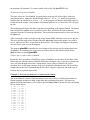
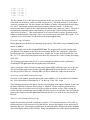
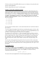
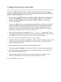
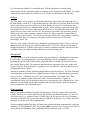
ESTIMATING FITNESS FUNCTIONS
USING THE CUBIC SPLINE
glms 4.0
glmsWIN 1.0
December 20, 2000
Dolph Schluter
Department of Zoology
University of British Columbia
Vancouver, B.C. Canada V6T 1Z4
[email protected]
I. GETTING STARTED .................................................................................................................... 2
Example 1: Survival and body size of house sparrows........................................................... 2
Example 2: Survival and body size of male human infants .................................................... 3
Example 3: Fitness with a categorical covariate ................................................................... 5
Running glms directly ............................................................................................................. 5
2. WHAT THIS PROGRAM DOES ..................................................................................................... 6
3. CHANGES FROM THE PREVIOUS VERSION OF GLMS ................................................................... 7
4. WHAT'S INCLUDED WITH THE PACKAGE ................................................................................... 8
5. ADDITIONAL EXPLANATION OF INPUT AND OUTPUT ................................................................. 9
Minimizing the GCV score...................................................................................................... 9
Effective number of parameters ............................................................................................ 10
Fitting a covariate................................................................................................................. 10
Bootstrapping........................................................................................................................ 11
Binomial/Poisson glm settings.............................................................................................. 11
Outliers. ................................................................................................................................ 12
Why splines? ......................................................................................................................... 12
Other programs..................................................................................................................... 12
6. PROGRAM COMPILATION NOTES ............................................................................................. 13
7. ACKNOWLEDGMENTS............................................................................................................. 14
8. REFERENCES .......................................................................................................................... 14
I. Getting started
This section gives a quick demonstration of how to run the spline program using the
demonstration data sets. The simplest way is to run the program glmsWIN, which takes user
settings typed to the screen. It then runs glms, the main program to estimate a fitness function
using the cubic spline. Finally, glmsWIN grabs the main results from the output file and
displays them graphically. Details and hints regarding user settings are given in a later section.
To begin, delete the file glms.in (if it is present) from the directory containing the two programs.
Example 1: Survival and body size of house sparrows
The first data set contains measurements of body size (first principal component) and survival of
49 female house sparrows collected by Bumpus (1899) during a winter storm. The data are in the
included file demo1.dat. The first few lines of data are shown below:
0
0
0
0
1
0
…
2.98746
3.05050
3.06120
3.10031
3.10056
3.10513
The first column (Y) give the fitness measurement, in this case survival (0 or 1). The second
column (X) is the trait, in this case a composite measure of body size. The goal is to estimate the
relationship between the probability of survival and size.
First run: range of lambdas
Double click on the program file glmsWIN10.exe. This will open a MS-DOS window and also
a Windows widget with default user settings tailored to the first example data set (binomial
fitness data, no covariate, “Y X” data format). Leave the program option set at “range of
lambdas”. After viewing the settings, click “OK”, which will launch the program glms. Keep
the DOS window up front to monitor program progress. When the program finishes running, a
graphics window will open up depicting program results.
The plot depicts the performance of different values of the smoothing parameter, lambda,
displayed along the X-axis of the plot. The Y-axis of the plot gives the cross-validation scores of
each lambda tested. These scores give a measure of prediction error, akin to least squares. The
idea is to choose the lambda having the lowest cross-validation score. In this data set, a lambda
value of −6 seems to be the best.
These and other output details are saved in the file glms.out and in a second file of your choice
if you type a different output file name in the corresponding box. Output files are overwritten
on each subsequent run of the program, so choose a different output file name or rename
glms.out after each run if you wish to save results.
After viewing the results, click the second mouse button (MB2) while the cursor is over the plot.
This will send the graph to the Windows Metafile glms.wmf, which can be imported into
Powerpoint, Word, etc. (rename the graph if you wish to save it, otherwise it will be overwritten
on the next run). The widget will also return to begin another run. (If you click the “×
×” instead,
the program will terminate. To resume, double-click on the file glmsWIN10.exe).
Second run: fixed value of lambda
This time, select the “fixed lambda” program option in the top left of the widget. In the box
immediately below, change the default lambda value of “−10” to “−6”, which is the optimal
lambda value (be careful not to set it to “−−6”, as the program will not like the double negative).
Further down the widget, set the number of bootstrap replicates to 50. Then click “OK” to begin
the run.
The resulting graph depicts the fitness function corresponding to the optimal lambda. The dotted
lines indicate one standard error of predicted values above and below the fitness function,
computed from the 50 bootstrap replications. These and other output details are also saved in the
file glms.out.
After viewing the results, click the second mouse button (MB2) while the cursor is over the plot.
This will send the graph to the Windows Metafile glms.wmf (rename the graph if you wish to
save it, otherwise it will be overwritten on the next run). The widget will reappear to begin the
next run. Press “Quit” to exit the program.
The program glmsWIN remembers the user settings of the previous run by storing them in the
file glms.in. If something goes wrong and you need to return to the default settings, delete
glms.in before re-running glmsWIN.
Further runs: try other values of lambda.
Repeat the above procedure with different values of lambda to see the effect on the shape of the
fitness function. Smaller values of lambda will lead to a bumpier curve; at the lower extreme, the
curve will pass through each of the Y-observations. Larger values of lambda will yield a
smoother curve; at the upper extreme, in the case of normally-distributed errors, the fit will be a
straight line (in the case of binomial data the fit will be a logistic regression, and in the case of
Poisson data, a log-linear regression).
Example 2: Survival and body size of male human infants
The second data set consists of measurements of survival to 28 days of male human infants in
British hospitals in relation to birth weight (lbs) and gestation period (days). The data were
gathered by Karn and Penrose (1951) and are given in demo2.dat. The first few lines of the data
file are shown below:
0.000
0.000
0.000
0.000
0.000
0.000
0.000
0.000
0.000
0.000
0.000
0.000
1.000
0.000
1.0
1.0
5.5
1.0
1.5
1.5
2.0
2.5
3.5
4.5
1.0
2.0
4.5
2.0
155
165
170
180
180
185
185
185
185
185
190
190
190
195
1
2
1
1
2
1
1
2
1
1
1
3
1
1
0.000
0.000
0.000
0.000
1.000
2.5
1.0
2.0
3.0
6.0
195
200
200
200
200
1
1
3
3
1
…
The first column (Y) give the fitness measurement, in this case survival. The second column (X)
is the main trait of interest, in this case birth weight (in lbs.). The third column (C) is the linear
covariate, gestation time. The last column is the number of infants N having the indicated values
of X and C (this format is useful when there are many tied observations). Y in this case
represents the mean Y-value of the N individuals having the same values for X and C. The goal is
to estimate the relationship between probability of survival and X while holding constant the
value of the covariate, C. (We assume that the fit of survival to the covariate, gestation period,
follows a standard logistic regression. That is, the covariate is not also fitted with a spline. To fit
a spline to two or more traits, use the multivariate program pp instead.)
First run: range of lambdas
Delete glms.in from the directory containing the programs. Then make a copy of demo2.in and
rename it glms.in.
To begin, double click on the file glmsWIN10.exe. The program will read the settings in the
new glms.in. The changes to note from the last example include: the “continuous” option has
been selected in the Covariate Information box; “demo2.dat” is types in the Data File box, and
the “Y X C N” option has been selected in the Data File Structure box. After viewing the settings,
click “OK”.
The resulting graph shows that the GCV score is minimized at 0 (this can be confirmed by
examining the file glms.out after the graph has been discarded.
After viewing the results, click the second mouse button (MB2) while the cursor is over the plot.
This will send the graph to the Windows Metafile glms.wmf. Rename this file if you wish to
save the plot file for later use. Clicking MB2 will also re-launch the widget for the next run.
Second run: fixed lambda without bootstraps
Select the “fixed lambda” program option and set the lambda to “0” in the Enter Fixed Lambda
box. Leave the number of bootstraps at “0” for this run. Click “OK” to run
The resulting graph depicts the fitness function corresponding to the optimal lambda. In this case
the fitness function for the trait, birth weight, is “adjusted” for the covariate (gestation time).
Predicted values for all observed levels of the covariate are shown as dots. After viewing the
results, click the second mouse button (MB2) while the cursor is over the plot. This will send the
graph to the Windows Metafile glms.wmf. Rename this file if you wish to save the plot file for
later use.
Third run: fixed lambda with bootstraps
Repeat the procedures from the second run except use “50” bootstrap replicates. Click “OK” to
run the program (it will run more slowly than the last, because the program is now analysing 50
bootstrap data sets). The resulting graph depicts the adjusted fitness function, the spline obtained
after removing the effects of the covariate, along with standard errors of the adjusted predictions.
Click the second mouse button (MB2) while the cursor is over the plot to close and send it to the
Windows Metafile glms.wmf.
When the widget returns, press “Quit” to exit the program.
Example 3: Fitness with a categorical covariate
This last example involves a fictitious data set created to illustrate a spline fit that adjusts for a
category-type covariate. Fitness measurements are assumed to be normally distributed about the
fitness function. The covariate is a category variable having three levels, 1994, 1995, and 1996,
representing three years of study. (Note that levels of a category-type covariate must be given
as numbers. Using alphabetic characters or other symbols will cause an error when the
data file is read by the program). The data are in the file demo3.dat. The first few lines of the
data file are listed here:
9.1
9.2
8.4
9.4
8.7
9.3
10.6
9.5
-0.95
-0.90
-0.87
-0.84
-0.82
-0.80
-0.78
-0.73
1995
1995
1995
1995
1995
1995
1995
1995
…
The first column is the fitness measure, Y, the second column is the trait X, and the last column is
the covariate, C.
To run the example, delete glms.in from the directory containing the programs. As before, make
a copy of demo3.in and rename it glms.in. Then double click on the file glmsWIN10.exe. This
will launch a widget having the user settings listed in the new glms.in.
The settings are for a fixed lambda of −3, which is the optimal lambda according to a previous
analysis (not shown) testing a range of lambdas, and no bootstrapping. Other settings to notice in
the new window include: the “category” option has been selected in the Covariate Information
box; “demo3.dat” is types in the Data File box; the “X Y [C]” option has been selected in the
Data File Structure box; and the “normal” Model is selected. After viewing the settings, click
“OK”.
The dots in the resulting graph depict the predicted values for each level of the covariate (three
levels in all). The curve is the “adjusted” fitness function, which shows the predicted relationship
between Y and X after removing the effects of the covariate (gestation time). Press “Quit” to exit
the program.
Running glms directly
It is possible to run glms without running glmsWIN. To do this, you will need to open and edit
the user settings in the file glms.in. You will also need to open an MS-DOS window and change
the directory to that containing the programs. Then run glms by executing the following
command in the MS-DOS window:
glms40 < glms.in
The results will be stored in glms.out but will not be displayed graphically.
2. What this program does
This program estimates a fitness function (or other regression surface) using the cubic b-spline, a
method summarized in Schluter (1988). The method assumes that we are trying to estimate a true
fitness function, f, that depends on a single trait variable X as
Y = f(X) + random error.
Y is a measure of individual fitness, such as survival, reproductive success, or other measure of
performance. f(X) is the average fitness of all individuals having the trait value X. The goal is to
estimate the surface f without making any prior assumptions about its shape, except that it is
smooth. Three different random error distributions are accommodated: normal, binomial (e.g.,
binary measurements such as survival), and Poisson (e.g., number of mates). For binomial and
Poisson errors, estimates of the surface use the iterative methods of generalized linear models.
For example, for survival data, we estimate g(X) instead of f(X), where g(X) is
exp{ f(X) }
g(X) = Prob(Y=1 | X) = 
1 + exp{ f(X) }
For Poisson data (e.g., number of mates),
g(X) = exp{f(X)}.
The basic goal when running the program is to estimate the best spline fit by searching over a
range of values of the smoothing parameter lambda (the program uses a log scale for lambda).
The best fit is given by the lambda value minimizing the generalized cross-validation function
(GCV score), which is a measure of prediction error.
To intuit what the program does, think of the spline as roughly analogous to a running mean
(more accurately, a running regression), where lambda represents the width of the sliding
window. Imagine placing a window, representing a span of possible X-values, along the X-axis
centered on a single value of X. Carry out a linear regression of Y on X using only the X
observations (and associated Y-values) that fall within the window. Use this local regression to
predict Y corresponding to the X value at the center of the window. Slide the window along Xaxis over to another X value of and repeat the above steps. The series of predicted Y-values is our
estimate of the fitness function. If the window is narrow (corresponding to a small value of
lambda) then the fitness function will be bumpy. If the window is wide, corresponding to a large
lambda, the function will be much smoother.
The program can simultaneously fit a single covariate if one is present. The covariate is not fit
with a spline, but rather is fit using conventional regression and anova methods (logistic or loglinear regression/anova in the case of binomial or Poisson Y-values, respectively). The spline
and the covariate are fit simultaneously using an iterative procedure called backfitting.
Splines can be fit to more than one X-variable in a multivariate analogue of this program (pp)
available at www.zoology.ubc.ca/~schluter/splines.html.
3. Changes from the previous version of glms
Version 4.0 of glms contains a number of changes from earlier versions. One of the changes
affects the required data format, with the result that you will not be able to use your previous
data files without modification (see item 3 below).
1. The new program, glmsWIN, provides a Windows interface. MS-DOS fans can bypass this
program and run glms by executing the command “glms40 < glms.in” in an MS-DOS
window. The program glms does not solicit input settings from the user as in previous
versions of the program.
2. Version 4.0 of glms makes use of extended and expanded memory, and hence is free of the
conventional memory restriction that limited the size of data sets that could be handled by
earlier versions of GLMS. The distributed executable program can handle a file of up to
10,000 cases. This value can be increased if necessary by modifying the source code and
recompiling. Compilation notes are given in a later section.
3. The format of input data files is changed from “X Y …” to “Y X …”. In other words, Y must
now be in the first column of the data file and X is the second column. This change was made
so that glms conformed to the input format of the multivariate program, pp.
4. The new version allows simultaneous fitting of a single covariate.
5. Lambda has been re-scaled. The best lambda for a data set analysed with the previous version
of the program will not be the best lambda when the same data are re-analysed with the
present version of the program.
6. Bootstrap standard errors are provided only when lambda is fixed.
7. The programs pav and breaktie are discontinued. If there is demand I will bring them back.
8. The option of generating and inspecting just one bootstrap replicate has been removed. If
there is demand I will bring it back.
9. Upper and lower bounds have been placed on many of the internal variable to prevent
overflows and underflows, which in previous versions would cause a crash.
10. The manual has been revised.
4. What's included with the package
Executable files
These programs may be run on machines running Windows 95, 98, NT, and 2000.
glms40.exe is the main program for computing a cubic spline using generalized crossvalidation.
glmsWIN10.exe is the program that takes user settings from the screen and then runs the
program glms40.exe.
Data files
demo1.dat, demo2.dat, demo3.dat contain the example data sets.
Input files
demo1.in, demo2.in, demo3.in contain user settings for the example data sets.
Source code
glms.f contains the fortran77 source code for the program glms.
glmswin.f contains the fortran77 source code for the program glmsWIN.
Help file
glms.manual.pdf is the present manual.
5. Additional explanation of Input and output
The present section provides advice on settings and interpretation of output. This will also help
troubleshooting if problems arise.
If things start to go badly wrong and you are unable to avert repeated crashes, the best thing to do
is delete the file glms.in and start again. On the next run the program glmsWIN will revert to
its default settings.
Minimizing the GCV score
Range of lambdas.
The program allows the user to search for the value of the smoothing parameter that minimizes
the GCV score (and ordinary cross-validation score OCV; the difference between the two is
explained below). A lower limit of −10 and an upper limit of 10 are the defaults, and this range
should work for most purposes. Lambda values below −10 will generally yield a very rough
fitness function with too many effective parameters, which should be viewed with suspicion. At
the other extreme, a lambda of 10 will yield a function close to the smoothest possible (a straight
line, in the case of normal errors). Increasing lambda beyond this value will make little
difference to the estimate. For this reason it will not often be necessary to go outside the default
limits. On the other hand using the default limits of -10 and 10 will yield only a coarse search. In
Example 1, the best lambda was found to be −6. A refined the search using the limits −7 and −5
would have shown the value of −5.6 to be better still.
Cross-validation.
The method of cross-validation involves deleting an observation, computing the fitness function
with the remaining observations, and then determining how accurately the missing point was
predicted. The difference between the Y-value of the missing observation and the predicted Y is
the prediction error. This is repeated for all data points, yielding a prediction error for each one.
Both the GCV score and the OCV score are calculated from the weighted sum of squared
prediction errors, but they are computationally slightly different.
The goal is to choose a value of lambda to minimize the cross-validation score. The GCV score
has some advantageous statistical properties and is therefore usually preferred to the OCV score.
However, the two give similar results and I provide them both (only the GCV score is given
when there is a covariate). OCV will sometimes give a clear minimum when GCV does not, in
which case I recommend using the OCV score instead. In my experience this problem sometimes
arises with small sample size (low number of unique X-values). It may also happen when the
frequency distribution of X-values is skewed, or when there are severe outliers in X. Some of
these problems may be fixed by transforming X prior to analysis (e.g., by using a logtransformation in the case of right-skewed data).
Analysis of some data sets yields more than one minimum in the GCV score. An example is the
following:
Range of lambdas
GCV score (solid) and OCV score (dotted)
0.618
0.608
e 0.597
r
o
cS
0.587
0.576
0.566
-13.000
-10.400
-7.800
-5.200
ln(lambda)
-2.600
-0.000
Here, lambdas of both −6 and −10.5 correspond to minima in the GCV score. In such instances I
recommend the conservative approach, which is to prefer the largest lambda corresponding to a
minimum in the GCV score. In other words, choose the lambda of −6, not −10.5.
Effective number of parameters
The “effective” number of parameters is provided on output. This is not the real number of
parameters in the cubic spline equation, but is instead a quantity describing the complexity of the
shape of the function. The minimum “effective” number of parameters is 2. This is achieved
when lambda is large and the fit is a straight line regression (logistic regression in the case of
binomial errors; log-linear in the case of Poisson errors). A fit with 3 effective parameters will
have a simple curvilear shape, such as a parabola. An estimated function having many effective
parameters should be viewed with caution, especially when sample size is not large: a simpler
function may explain the data just as well. The maximum number of effective parameters is
equal to the number of unique X-values in the data (e.g., 49 in the data set demo1.dat). Such a
fit, which zig-zags up and down repeatedly as it passes through every individual data point, has
no generality. Generality is one of the motivations behind the goal to maximize the accuracy of
prediction by choosing a lambda that minimizes the GCV score.
Fitting a covariate
The program will simultaneously fit a single covariate. By “covariate” I mean a second
independent variable that needs to be taken into account when fitting Y to X. The covariate may
be a continuous variable like X (e.g., body mass), or it may be a category variable (e.g., year, sex,
age class). The distributed executable program allows up to 20 levels for a category-type
covariate. In the data file, the categories must be given as numbers rather than alphabetical
or other symbols. The program is unable to read non-numerical symbols.
This covariate is not fitted with a spline, but rather is fitted with a conventional linear regression
or anova (logistic and log-linear regression in the case of binomial and Poisson data). The fit is
“simultaneous” rather than sequential. That is, the program finds the combination of spline and
covariate regression that best fits the data, rather than fitting one variable first and then fitting the
second variable to the residuals from the first. The simultaneous fit is carried out using the
method of backfitting. A total of five backfit iterations is carried out for each lambda tested.
As with ordinary analysis of covariance, the true fitness function will be more accurately
measured if different levels of the covariate have the same range of X-values. This minimizes the
correlation between X and the covariate.
Bootstrapping
The bootstrap is a useful technique for estimating the sampling variability of a fitted function. It
is recommended that at least 50 bootstrap replicates are used. You must provide an integer
random number seed. Any positive or negative integer except 0 should work. A decimal or other
symbol in the random number seed will cause the program glms to crash. Running the program
on a given data set using the same random number seed will yield precisely the same sequence of
random errors in the set of bootstrap samples. It is therefore recommended that you change the
seed each time you run the program.
The method used here begins by fitting the data with a specified lambda value, preferably the
best (the lambda minimizing the GCV score). This fitted function is then be used to generate all
the bootstrap samples. A single bootstrap sample is created by taking the predicted Y-value
(based on analysis of the original data) for each unique X and adding a random error. For
example, if the data conform to the normal model, then a normally-distributed random error is
added to each predicted Y to yield a new “ bootstrap value” for Y, where the variance of the
random error is set to equal the variance of the residuals of the initial spline fit (the spline fit to
the real data). The full set of bootstrap Y-values, one for each X, is then fitted with a spline using
the same value of lambda as the initial fit to the data. The predicted Y-values from this analysis
of the bootstrap values are saved and a new bootstrap sample is created as before. This process is
repeated multiple times, the number specified by the user during the run (e.g., 50). The standard
deviation of predicted bootstrap Y-values is then calculated for each unique X; this is the standard
error of the prediction. The output of the program includes the values corresponding to one
standard deviation above, and one standard deviation below, the predicted Y-values from the
initial spline fit of the data.
In the case of binomial or Poisson errors, the standard deviation of the bootstrap predicted Yvalues is calculated out on the logistic scale (Y’ = ln[Y/(1-Y)] ) or log-linear scale (Y’ = ln[Y] ),
respectively, and then transformed back to the same scale as Y. For this reason the upper and
lower limits corresponding to one standard deviation may not be symmetric about the predicted
Y.
Binomial/Poisson glm settings
In the case of binomial and Poisson errors, two other settings are requested. The first is the
convergence tolerance and the other is the maximum number of iterations. I recommend using
the default settings.
The regression for binomial and Poisson data requires iteration because the variance of the
residuals is expected to be heterogeneous, and changes with different predicted values of Y. The
regression must therefore weight each observation according to expected error variance.
However, the weight itself is estimated from the predicted Y-values obtained from the spline. The
glm method thus involves selecting initial arbitrary weights, fitting the spline, then recalculating
the weights, fitting another spline with these new weights, and so on, until improvements from
subsequent iterations are marginal. The convergence tolerance specifies what is considered
“marginal improvement”.
Five iterations, the default, is a reasonable start. If all the iterations are used up before
improvements become marginal (number of iterations used is indicated on the output), you might
wish to increase the number of iterations to see if it makes any difference to the outcome.
Outliers.
The cubic spline is less sensitive to outliers than parametric regression in one important way. If
the data include a cloud of (Y,X) observations plus one odd point well removed from the rest (the
outlier), then linear regression will try very hard to fit that one point. This will influence the
slope of the regression even within the cloud of points. That is, ordinary regression will give the
best global fit even if it means compromising the local fit (i.e., that within the main cloud). The
spline, however, finds a more local best fit. The presence of an outlier will not usually greatly
influence the form of the regression within the cloud. The effective number of parameters is a
measure of how local is the fit. Two effective parameters will have the same problem as ordinary
linear regression. However, functions with greater number of parameters will provide
increasingly “local” fits.
However, even a spline will tend to pass through the outlying point (clearly, if there is only one
data point lying out from the rest, the best prediction for Y is Y itself). This just means that not
enough information is available in that region to make a confident prediction, and hopefully this
would be reflected in a high bootstrap standard error at the outlying point.
Why splines?
The cubic spline is a useful method to estimate regression functions, including fitness functions.
It is referred to as a “nonparametric” regression method because no assumptions are made
regarding the specific form of the function, other than that it is smooth. The function may take
any form the data warrant. The parameters that describe the equation for the cubic spline itself
are not of interest. Instead, the goal is to generate a set of predicted Y’s that best summarizes the
relationship between Y and X.
Alternative methods exist for calculating nonparametric regression surfaces. The most frequently
used alternatives are those based on weighted moving averages or weighted moving regressions
such as “lowess” (Chambers et al. 1983) and “kernel estimation” (Silverman 1986). These
techniques are related to splines (Silverman 1986). One main advantage of splines is
computational: there exists an analytical short-cut to computing the cross-validation score. These
short-cuts are unavailable for the other estimates, and one must tediously delete one point at a
time to compute the cross-validation scores.
Other programs
Many of the standard statistical packages for data analysis will also compute cubic spline fits.
Usually, however, they require normal errors and will not easily handle binomial (e.g., survival)
or Poisson errors (e.g., number of mates). Usually they will also not provide a cross-validation
score that would allow the user to choose the best lambda in an objective way. Finally, most will
not allow a covariate to be fitted simultaneously.
The best standard statistical package for fitting cubic splines (and other nonparametric regression
methods) is S-Plus (Mathsoft 1999). The program glms is a special case of a generalized additive
model (Hastie and Tibshirani 1990), implemented by the function “gam” in S-Plus.
6. Program compilation notes
The source codes for the programs glms and glmsWIN were written in Fortran 77 and are
contained in the files glms.f and glmswin.f. Below I describe how the code was compiled so
that you may repeat the effort if necessary. You will need to recompile glms if you wish to
increase or decrease the maximum number of cases that can be handled (currently 10000) or the
maximum number of levels of the covariate (currently set to 20). These changes can be made to
NMAX and MMAX in the first PARAMETER statement of the source code in glms.f.
I compiled the source code using the GNU Fortran 77 compiler g77 for Win95/98 and Windows
NT included in the distribution package gcc-2.95. g77 is just a front-end for gcc, the GNU
C/C++ compiler. The package consisting of gcc and g77 is available free at
http://www.xraylith.wisc.edu/~khan/software/gnu-win32/gcc.html. I used the Mingw32 version
of the CRTDLL runtime libraries, gcc-2.95.2-crtdll.exe.
If you wish to edit and recompile the source code, first install gcc-2.95 on your computer by
following the instructions accompanying that program. After you install, and have modified your
PATH statement in AUTOEXEC.BAT to include the gcc-2.95 command directory, compile the
source code in glms.f using the command:
g77 -fugly-assumed glms.f -o glms40.exe
Recompiling the program glmsWIN requires that you also install the DISLIN library of Win32
graphics routines. These routines are available free at http://www.linmpi.mpg.de/dislin (be sure
to download the version corresponding to gcc-2.95 and the Mingw32 version of the CRTDLL
runtime library). Install DISLIN by following the instructions accompanying that program,
including the addition of the command “set DISLIN=C:\[path to dislin directory]” in the
AUTOEXEC.BAT file. Then compile the source code in glmswin.f using the command:
g77 -fugly-assumed glmswin.f %DISLIN%\dismg7.a -luser32 -lgdi32
-lcomdlg32 -o glmsWIN10.exe
7. Acknowledgments
This version of glms is based on routines initially written by Dr. Douglas Nychka (Statistics
Department, NCSU, Raleigh N.C.).
8. References
Bumpus, H. C. 1899. The elimination of the unfit as illustrated by the introduced sparrow,
Passer domesticus. Biol. Lect. Woods Hole Mar. Biol. Sta 6: 209−226.
Chambers, J. M. , W. S. Cleveland, B. Kleiner, and P. A. Tukey. 1983. Graphical methods for
data analysis. Wadsworth, Belmont, California.
Hastie, T. J. and R. J. Tibshirani. 1990. Generalized additive models. Chapman and Hall,
London.
Karn, M. N. and L. S. Penrose. 1951. Birth weight and gestation time in relation to maternal age,
parity and infant survival. Ann. Eugen. 16: 147−164.
Mathsoft, Inc. 1999. S-Plus 2000 language reference. Seattle, Washington.
Mitchell-Olds, T. and R. G. Shaw. 1987. Regression analyses of natural selection: statistical
inference and biological interpretation. Evolution 41: 1149−1161.
Schluter, D. 1988. Estimating the form of natural selection on a quantitative trait. Evolution 42:
849–861.
Silverman, B. W. 1986. Density estimation for statistics and data analysis. Chapman and Hall,
London.