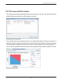
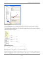
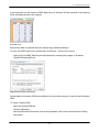
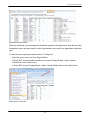
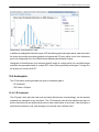
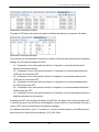
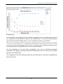
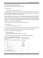
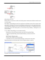
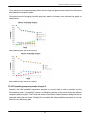
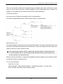
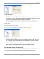
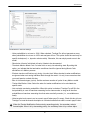
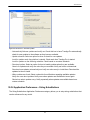
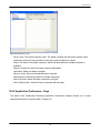
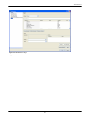
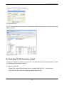
1
TreeAge Pro 2012 User's Manual
TreeAge Pro 2012
TreeAge Pro 2012 User's Manual: TreeAge Pro 2012
© 2012 TreeAge Software, Inc.
Table of Contents
1. Introduction ........................................................................................................................................ 1
Welcome to TreeAge Pro ...............................................................................................................1
TreeAge Pro Interface .................................................................................................................... 1
Optional modules ............................................................................................................................2
Integration with other software ....................................................................................................... 2
Installation and system requirements .............................................................................................2
Cross-Platform Compatibility .......................................................................................................... 3
Get technical support ..................................................................................................................... 3
File compatibility ............................................................................................................................. 4
Manual structure .............................................................................................................................5
What's New in TreeAge Pro .......................................................................................................... 5
2. Decision Analysis Primer .................................................................................................................. 8
What is decision analysis? .............................................................................................................8
A simple problem: How should I invest $1000? ...........................................................................10
Decision trees ...............................................................................................................................11
Dependency diagrams ..................................................................................................................13
Further reading ............................................................................................................................. 13
Example Models ........................................................................................................................... 14
3. TreeAge Pro Interface .....................................................................................................................15
TreeAge Pro Workbench ..............................................................................................................15
Perspectives ................................................................................................................................. 17
Tree Diagram Editor ..................................................................................................................... 18
TreeAge Pro Views ...................................................................................................................... 20
4. A Decision Tree Tutorial ................................................................................................................. 24
Constructing a tree ....................................................................................................................... 24
Entering payoff values ..................................................................................................................27
Entering probabilities .................................................................................................................... 30
Setting calculation and numeric formatting preferences .............................................................. 32
Calculating the tree ...................................................................................................................... 33
What's next? ................................................................................................................................. 34
5. Dependency Diagrams .................................................................................................................... 36
Dependency diagrams ..................................................................................................................36
Constructing a dependency diagram ........................................................................................... 36
Creating and selecting nodes .......................................................................................................37
Entering the node label ................................................................................................................ 38
Adding arcs ...................................................................................................................................38
More editing options ..................................................................................................................... 40
Dependency Properties View ....................................................................................................... 41
6. Managing Projects and Documents ................................................................................................ 43
Create a project ............................................................................................................................43
Tutorial examples project ............................................................................................................. 44
Working within a project ...............................................................................................................45
Additional information on Projects View .......................................................................................45
Saving files ................................................................................................................................... 45
7. Printing and Presenting Trees ........................................................................................................ 46
Printing ..........................................................................................................................................46
Exporting Pictures ........................................................................................................................ 47
8. Analyzing Decision Trees ................................................................................................................49
Numeric Formatting ...................................................................................................................... 49
Expected values ........................................................................................................................... 49
Roll back .......................................................................................................................................50
Rankings ....................................................................................................................................... 52
Standard deviation ........................................................................................................................53
Discrete simulation/microsimulation ............................................................................................. 54
Probability distributions .................................................................................................................56
Expected value of perfect information (EVPI) .............................................................................. 61
Other Analyses ............................................................................................................................. 65
9. Graph Windows ...............................................................................................................................67
BIRT Project ................................................................................................................................. 67
Customizing graphs/charts ........................................................................................................... 67
Customizing probability distribution graphs ..................................................................................74
Customizing cost-effectiveness graphs ........................................................................................ 77
Customizing line graphs ............................................................................................................... 78
Customizing scatterplot graphs .................................................................................................... 82
Printing, exporting and saving graphs ..........................................................................................88
10. Tree Calculation Methods and Preferences ..................................................................................90
Changing what the tree calculates ...............................................................................................90
Calculations using multiple attributes ........................................................................................... 95
Roll back analysis options ............................................................................................................97
Regional/international numeric settings ........................................................................................99
Overriding the optimal path at selected nodes .......................................................................... 100
11. Selecting Subtrees and Multiple Nodes ...................................................................................... 102
Selecting a subtree .....................................................................................................................102
Selecting multiple, unrelated nodes ........................................................................................... 102
Selecting multiple nodes by characteristic ................................................................................. 103
12. Making Changes to Tree Structure ............................................................................................. 105
A note on tree terminology .........................................................................................................105
Tree-building commands – a review .......................................................................................... 105
Editing a single node vs. subtrees ............................................................................................. 106
Inserting nodes/branches ........................................................................................................... 106
Moving/reordering nodes ............................................................................................................ 109
Deleting nodes/branches ............................................................................................................ 111
Cut, copy, and paste nodes and subtrees ................................................................................. 111
Cut, copy, and paste text ........................................................................................................... 116
Multiple clipboards ......................................................................................................................117
Undo and Redo .......................................................................................................................... 118
Find and replace text, formulas, and values .............................................................................. 118
Using the Probability Wheel View .............................................................................................. 121
13. Annotating the Tree .....................................................................................................................123
Node label options ..................................................................................................................... 123
Label nodes ................................................................................................................................ 125
Notes and arrows ....................................................................................................................... 126
Node comments ......................................................................................................................... 131
14. Tree Display Preferences and Options ....................................................................................... 134
Collapsing/hiding subtrees ..........................................................................................................134
Aligning selected nodes ............................................................................................................. 135
Displaying terminal columns/roll back columns ..........................................................................136
Other tree display preferences ...................................................................................................138
15.
16.
17.
18.
19.
20.
Changing fonts ........................................................................................................................... 142
Introduction to Variables and Sensitivity Analysis .......................................................................144
Sensitivity analysis background ................................................................................................. 144
Using variables in a tree ............................................................................................................ 145
Performing one-way sensitivity analysis .....................................................................................153
Sensitivity analysis thresholds ....................................................................................................156
Working With Variables ...............................................................................................................159
Variable Properties View ............................................................................................................ 159
Variable Definitions View ............................................................................................................164
Define Variable Dialog ................................................................................................................169
Variable Categories .................................................................................................................... 170
Sensitivity Analysis Variable Properties ..................................................................................... 174
Sensitivity analysis correlations ..................................................................................................174
Variables testing tools ................................................................................................................ 175
Formula Editor ............................................................................................................................ 178
Variable Definition Arrays ...........................................................................................................178
Building Formulas Using Variables and Functions ......................................................................182
Quantity expressions in a model ................................................................................................182
Formula Editor ............................................................................................................................ 182
Auto-fill ........................................................................................................................................ 184
User-defined python functions ....................................................................................................186
Variable formula examples .........................................................................................................186
Using mathematical, statistical, and other functions .................................................................. 192
Arithmetic functions .................................................................................................................... 193
Financial/discounting functions ...................................................................................................194
Miscellaneous functions ..............................................................................................................195
Using mathematical, statistical, and other functions .................................................................. 196
Recursive variable definitions .....................................................................................................196
Operators .................................................................................................................................... 199
Keywords .................................................................................................................................... 202
More Sensitivity Analysis Tools .................................................................................................. 203
Analyzing variables with multiple definitions .............................................................................. 203
Tornado diagrams ...................................................................................................................... 206
Two-way sensitivity analysis ...................................................................................................... 210
Three-way sensitivity analysis .................................................................................................... 213
Threshold analysis ......................................................................................................................214
Analyzing correlated variables ................................................................................................... 216
Additional sensitivity analysis topics .......................................................................................... 218
Monte Carlo Simulation, Distributions and Probabilistic Sensitivity Analysis ...............................220
Uses of Monte Carlo simulation in modeling ............................................................................. 220
Creating distributions .................................................................................................................. 223
Performing probabilistic sensitivity analysis ............................................................................... 228
Simulation options ...................................................................................................................... 238
Customizing simulations ............................................................................................................. 248
Two- and three-dimensional simulations ....................................................................................250
Distribution Functions, Options and Types ................................................................................. 253
Distribution functions .................................................................................................................. 253
Distribution options ..................................................................................................................... 254
Distribution Formulas ..................................................................................................................261
Sampling from tables during Monte Carlo simulation ................................................................ 261
21. Creating and Using Tables ......................................................................................................... 265
Creating and editing tables ........................................................................................................ 265
Referencing tables in formulas ...................................................................................................270
Model tables and global table files ............................................................................................ 272
Importing tables from older versions of TreeAge Pro (2009 and earlier) ................................... 274
The All Tables Report ................................................................................................................ 277
Managing tables using the Excel module .................................................................................. 278
Linking a table to an ODBC data source ................................................................................... 278
22. Stored Analysis Abstracts and Sequences ................................................................................. 285
Using stored analyses ................................................................................................................ 285
Sequencing stored analyses ...................................................................................................... 287
23. Linking with Excel and Other Applications ..................................................................................290
Dynamic linking with Excel via BiLinks ...................................................................................... 290
Calculating payoffs using dynamic links: an example ................................................................ 291
24. Tools and Functions for Complex Trees .....................................................................................295
Working with very large trees .................................................................................................... 295
TreeAge Pro Workspace, Tree Explorer and Model Overview .................................................. 295
Viewing/editing document XML .................................................................................................. 299
Cloning subtrees .........................................................................................................................303
User-defined Python functions ................................................................................................... 311
Node(), Tree(), User(), Global() and other special functions ......................................................318
The Node() function ....................................................................................................................319
The Tree() function .....................................................................................................................322
The Command() function ............................................................................................................325
The Debug() function ..................................................................................................................327
The Seed() Function ...................................................................................................................327
The Global() and GlobalN() functions ........................................................................................ 327
The TrackerIncr() function .......................................................................................................... 329
List/matrix functions .................................................................................................................... 329
25. Advanced Chance Node Techniques and Options ..................................................................... 331
Using non-coherent probabilities ................................................................................................ 331
Sampling probabilities from a Dirichlet distribution .................................................................... 333
26. Bayes' Revision in Decision Trees ..............................................................................................337
An introduction to Bayes’ revision ..............................................................................................337
Bayes' Revision - Sensitivity/Specificity ..................................................................................... 339
Bayes' Revision - Grid ................................................................................................................342
27. Utility Functions and Risk Preferences ....................................................................................... 347
Risk preference: an illustration ...................................................................................................347
Risk preference curves ...............................................................................................................348
Creating a risk preference function ............................................................................................ 349
28. Using the Excel Module .............................................................................................................. 351
Edit model inputs in Excel ..........................................................................................................351
Tree Workbook ........................................................................................................................... 358
TreeAge Pro Object Interface .................................................................................................... 359
Exporting analysis output ........................................................................................................... 359
29. Using the TreeAge Pro Object Interface .....................................................................................360
Java vs. Other Programming Languages ...................................................................................360
Object Interface API Documentation .......................................................................................... 360
Connecting to the Object Interface via Java .............................................................................. 361
Connecting to the Object Interface via ActiveX ......................................................................... 364
30. The TreeAge Pro Player ............................................................................................................. 367
Creating a Player Model ............................................................................................................ 367
Creating the Player Model Interface .......................................................................................... 368
Using the Model Interface .......................................................................................................... 370
31. Building and Analyzing Cost-Effectiveness Models .................................................................... 371
Before you begin ........................................................................................................................ 371
Preparing a tree for cost-effectiveness calculations ...................................................................372
Performing cost-effectiveness analysis ...................................................................................... 378
Dominance and incremental cost-effectiveness ......................................................................... 380
One-way cost-effectiveness sensitivity analysis .........................................................................385
32. Cost-Effectiveness Modeling and Analysis Options .................................................................... 389
Net benefits calculations ............................................................................................................ 389
Multi-attribute weighted costs ..................................................................................................... 390
Inverting effectiveness calculations ............................................................................................ 394
CE roll back optimal path parameters ........................................................................................397
Thresholds and CE sensitivity analysis ......................................................................................399
Displaying incremental values during roll back .......................................................................... 409
33. Cost-Effectiveness Simulation Reports and Graphs ................................................................... 410
Basic CE statistics and simulation outputs ................................................................................ 410
Cost-effectiveness graphs .......................................................................................................... 414
Output Distribution graphs ..........................................................................................................415
Scatterplots ................................................................................................................................. 418
Acceptability and Net Benefits curves ........................................................................................424
Cost-effectiveness value of information (EVPI and EVPPI) ....................................................... 429
34. Building and Analyzing Markov Models ...................................................................................... 431
Markov modeling basics .............................................................................................................431
Building a Markov cycle tree in TreeAge Pro ............................................................................ 433
Analyzing a Markov model ......................................................................................................... 443
A note on microsimulation ..........................................................................................................449
A note on half-cycle correction .................................................................................................. 450
Cost-effectiveness Markov models .............................................................................................450
35. Markov Modeling Tools and Techniques .................................................................................... 454
Keywords, time-dependence, and discounting ...........................................................................454
Probability/rate conversion functions ..........................................................................................458
State/transition probability functions ...........................................................................................459
Assigning onetime costs and utilities ......................................................................................... 460
Cloning Markov models ..............................................................................................................465
Counting "time in state" with tunnels ......................................................................................... 469
Markov decision processes ........................................................................................................ 476
Dynamic cohort models ..............................................................................................................477
Extra Rewards ............................................................................................................................ 480
Other advanced Markov options ................................................................................................ 481
36. Individual-Level Simulation and Markov Models ......................................................................... 487
Notes on simulation terminology ................................................................................................ 487
Simulation and tracker variables ................................................................................................ 488
Tracker views and dialogs ......................................................................................................... 494
More notes on trackers .............................................................................................................. 497
Sampling individual-level distributions during simulation ............................................................498
Debugging simulations ............................................................................................................... 501
Parallel trials, discrete event simulation, and dynamic populations ........................................... 503
37.
38.
39.
40.
2-dimensional probabilistic sensitivity analysis using microsimulation ....................................... 514
Sensitivity Analysis and Microsimulation ....................................................................................517
Sequences and linear sensitivity analysis ..................................................................................519
Other aspects of microsimulation ...............................................................................................520
Markov Technical Details ............................................................................................................ 522
Model Documentation ..................................................................................................................523
Create Model Documentation Help File ..................................................................................... 523
Preferences ................................................................................................................................. 526
Tree Preferences ........................................................................................................................526
Tree Preference Sets ................................................................................................................. 527
Tree Preferences Dialog ............................................................................................................ 528
Calculation Method .....................................................................................................................529
Payoff Preferences ..................................................................................................................... 533
Numeric Formatting .................................................................................................................... 533
Roll Back .................................................................................................................................... 535
Risk Preferences ........................................................................................................................ 536
Regional Settings ....................................................................................................................... 538
Other Calc Settings .................................................................................................................... 540
Large Tree Optimizations ........................................................................................................... 542
Tables ......................................................................................................................................... 542
Arrows .........................................................................................................................................542
External Subtrees ....................................................................................................................... 542
Fonts ........................................................................................................................................... 543
Node Text/Comments .................................................................................................................544
Notes ...........................................................................................................................................544
Printing ........................................................................................................................................545
Terminal Columns ...................................................................................................................... 546
Terminal Nodes .......................................................................................................................... 547
Tree Editing/Layout .................................................................................................................... 548
Variables/Markov Info ................................................................................................................. 549
Dynamic Links ............................................................................................................................ 550
Identifying Variables ................................................................................................................... 551
Advanced Monte Carlo Options ................................................................................................. 551
Debugging ...................................................................................................................................551
Output Reports ........................................................................................................................... 553
Stored Analysis Abstracts and Sequences ................................................................................ 554
Application Preferences ..............................................................................................................554
Application Preferences Dialog .................................................................................................. 554
Application Preferences - Backup/Autosave .............................................................................. 555
Application Preferences - Display .............................................................................................. 556
Application Preferences - Automatic Updates ............................................................................557
Application Preferences - String Substitutions ........................................................................... 558
Application Preferences - Monte Carlo Distributed Processing ..................................................559
Application Preferences - Keys .................................................................................................. 560
Technical Details & Utilities .........................................................................................................562
Random number generator details .............................................................................................562
Report Output Files (*.rptx) ........................................................................................................ 562
Importing TP 2009 Simulation Output ........................................................................................563
TreeAge Pro News Reader ........................................................................................................ 564
1 Introduction
1. Introduction
This chapter serves as an introduction to TreeAge Pro and TreeAge Software, Inc.
1.1 Welcome to TreeAge Pro
TreeAge Pro has been designed to implement the techniques of decision analysis in an intuitive and
easy-to-use manner. It transforms decision analysis from a potentially tedious exercise into an easily
applied and highly visual means of:
1. Organizing the decision making process;
2. Analyzing the problem at hand; and
3. Communicating the structure of the problem, the nature of the uncertainties, and the basis for a
strategy recommendation.
If you are experienced in decision analysis, you will find TreeAge Pro easy to use following only a
cursory review of the software commands, although the richness of the program will become more
apparent with further study of the manual.
If you are looking for features added to recent releases, please refer to the What's New in TreeAge
Pro section of this chapter.
If you have no, or only limited, experience with decision analysis, TreeAge Pro will make it much easier
to learn. Go to the Decision Analysis Primer chapter for a basic decision analysis primer.
The organization of the rest of the manual is described in the last section of this Introduction Chapter.
1.2 TreeAge Pro Interface
TreeAge Software embarked on an ambitious project to rewrite the software within the Eclipse
development environment. Eclipse is a customizable development environment that allowed us to
incorporate many of its native features and third-party plugins into TreeAge Pro.
This new architecture not only improves the user interface and other components of TreeAge Pro 2011
and subsequent versions, but it also better positions us to add more functionality in future releases.
We hope you find that the newest version of TreeAge Pro is the most flexible, user-friendly version
of the software released to date.Prior users of TreeAge Pro will notice a big change in the TreeAge
Pro Interface.
For an introduction of the new interface, please refer to the TreeAge Pro 20 Interface chapter.
1
1 Introduction
1.3 Optional modules
TreeAge Pro follows a modular design. The "Core" module includes both decision tree functionality,
Monte Carlo simulation, multi-way sensitivity analysis, and much more. Additional features may be
added in the form of two optional add-ons: a Healthcare module and an Excel™ add-in module.
The TreeAge Pro Healthcare module integrates core decision analysis functionality with specialized
capabilities, including:
-
Markov cohort analysis
Individual-level, Markov simulation
Cost-Effectiveness analysis
Net Benefits analysis
Additional information available at http://www.treeage.com/products/overviewHealth.html
Healthcare Module Functions
The TreeAge Pro Excel/COM module can help:
- Automate the creation of Excel charts and reports from within TreeAge Pro
- Simplify the integration of spreadsheets and TreeAge Pro models via dynamic linking and/or
COM automation (i.e., macros)
- Edit input data in Excel
- Output analysis data to Excel
- Additional information available at http://www.treeage.com/products/overviewExcel.html
Excel Module Functions
The TreeAge Pro Suite includes all modules, including Healthcare and Excel/COM.
1.4 Integration with other software
In TreeAge Pro, users of the Excel/COM module gain access to powerful features that allow automation
of TreeAge Pro tasks via scripts and macros, in order to control updating and analysis of your models.
In addition, the embedded Python script interpreter has been improved, giving modelers easy access
to the powerful Python programming language.
1.5 Installation and system requirements
To install TreeAge Pro, please follow the installation instructions available on the installation CD and
from our web site: http://www.treeage.com/treeagepro/.
The installation instructions also cover hardware and software (operating system) requirements. See
the next section for information on how to contact TreeAge Software if you encounter difficulties during
installation.
2
1 Introduction
1.6 Cross-Platform Compatibility
TreeAge Pro 2011 and subsequent versions are built in the Eclipse architecture, which allows the
software to run on Windows, Mac, and Linux operating systems. There are different installers for each
OS available at our website. In each OS, the software should have a look and feel that for the most
part matches the native view for that OS.
Since TreeAge Pro 2009 and earlier versions ran only on the Windows OS, most of the instructions in
this manual describe Windows operations. There are some differences in commands/mouse-clicks on
Mac and Linux. The table below describes some of these differences.
Windows
Mac
Linux
Control + key
Command + key
?
Right-click
Option-click
Function keys
Fn key + function key
Command differences among operating systems
1.6.1 Mac Function Keys
Mac computers often use function keys to interact with the Mac Operating System. You can release
those function keys from their OS functions by changing settings in the System Preferences under the
category Keyboard. Specifically...
- Check the box to use F1, F2, etc. as standard function keys.
- Uncheck the box for active use of "Expose & Spaces" or "Mission Control".
1.6.2 Linux with GNOME Desktop Environment
If you use Unix-like operating systems with the GNOME desktop environment, you may be unable to
see the application's menu icons.
If you experience this problem:
- Start the gconf-editor.
- Select the checkbox in /desktop/gnome/interface/menus_have_icons
1.7 Get technical support
There are several ways to get help in using TreeAge Pro.
3
1 Introduction
1.7.1 Using the online help
TreeAge Pro installs with the online help you are currently reading. This help is quite extensive and
describes both modeling techniques and technical aspects of TreeAge Pro.
1.7.2 Web site resources
The support section of our web site includes a variety of information for users of the software:
http://www.treeage.com/support
http://www.treeage.com/support/technotes.html
http://server.treeage.com/treeagepro/support/demos.asp
1.7.3 Example models
Most chapters include tutorials and references to example models, which are installed on your computer
with TreeAge Pro. The Managing Projects and Documents Chapter describes how to access these
models.
1.7.4 E-mail and telephone support
If you are a registered user of TreeAge Pro with a current maintenance agreement, you are eligible for
free e-mail and telephone support; limited technical support is available if you are evaluating the trial
software. We would like to make your use or evaluation of the software as productive and pleasant
as possible. If you need help:
- Send an e-mail to [email protected].
- Call us at 1-413-458-0104, then 1 for Support.
(1-888-TREEAGE in US/Canada)
Access to technical support
1.8 File compatibility
TreeAge Pro 2011 introduced a new XML-based model file structure. Models in the new format will be
saved with the file extension .trex. Older *.tre and *.pkg files can be opened in TreeAge Pro 2011 and
subsequent versions. When you open a files from an older format, you are asked whether you want to
save the file in the new format or the old format. Not all features of TreeAge Pro 201x can be saved
in the TreeAge Pro 200x format.
4
1 Introduction
It is recommended that the old *.tre files are first saved as *.pkg files before opening them in
TreeAge Pro 201x. That way, the tables used by the model will be included with the new *.trex
document.
TreeAge Pro 201x can open trees created in previous versions of TreeAge Pro, as well as in DATA
Pro or DATA. However, unless your TreeAge Pro software includes the Healthcare module, access to
Markov and cost-effectiveness models created in either DATA or TreeAge Pro will be limited to viewing
the file.
Trees created in TreeAge Pro 201x are not directly backward-compatible with TreeAge Pro versions.
However, you can save models in an older format.
To save a model in an older TreeAge Pro format:
- Choose File > Save As from the menu.
- Select the file type TreeAge Pro 200x Package (*.pkg).
- Save the file.
Certain features not present in the earlier software will be lost in the conversion and, in any event, care
should be taken following conversion to confirm the accuracy of calculations.
1.9 Manual structure
This Manual is broken into several groups of chapters.
1. Getting Started with TreeAge Pro (starting with this chapter)
2. Working with Decision Trees (starting with the Analyzing Decision Trees Chapter)
3. Uncertainty and Variability: Using Variables, Tables, and Distributions (starting with the
Introduction to Variables and Sensitivity Analysis Chapter)
4. More Decision Tree Modeling and Analysis Options (starting with the Stored Analysis Abstracts
and Sequences Chapter)
5. Working with the Excel/COM Module (starting with the Connecting Spreadsheets and Trees
Using the Excel Module Chapter)
6. Cost-Effectiveness Analysis with Tree Age Pro Healthcare & TreeAge Pro Suite (starting with the
Building and Analyzing Cost-Effectiveness Models Chapter)
7. Markov Modeling, Analysis, and Simulation with the Healthcare Module (starting with the
Building and Analyzing Markov Models Chapter)
Sections of this manual
1.10 What's New in TreeAge Pro
This section identifies new features in the latest releases.
5
1 Introduction
1.10.1 TreeAge Pro 2012, Release 2
The following features were included in Release 2.0:
- Bayes Revision: Revise probabilities using Bayes' Theorem when your model includes imperfect
tests. This feature handles both sensitivity/specificity and a general m by n grid.
- Enhanced Search/Replace with Highlighting: This enhancements allows you to view and/or
replace the search results in a structured list. Search results are also highlighted in the model
structure.
The following features were included in Release 2.1:
- Object Interface Enhancements: The programming interface has been modified and enhanced
to provide better access to modeling objects and analysis output. It is now possible to access
secondary analysis output from Monte Carlo simulations and sensitivity analyses.
- Highlighting Expressions: The Variable Properties, Tracker Properties, Distributions and Tables
Views were enhanced to allow you to highlight the use of a model input within the Tree Diagram
Editor.
- Image Exports: Generate higher quality images of graphs and models for presentation and
publication.
- Improved User Interface Presentation: the Tree perspective has been rearranged to show the
most commonly used Views and to place similar views in the same area of the user interface.
Right-click on the Tree perspective and choose Reset to use the new format.
1.10.2 TreeAge Pro 2012, Release 1
This release introduced the following features:
- Sensitivity Analysis and Microsimulation: Run one-way sensitivity analysis and Microsimulation
at the same time. Microsimulation mean values are used as the expected values for each
variable value.
- Distributed Simulations: Use slave computers to speed up long simulations.
- Variable Definition Arrays: Create variable definitions with multiple expressions via an array. The
individual expressions are then referenced by index.
- Exportable summary report output: Output provided by the Markov Cohort Summary Report and
the Cost-Effectiveness Text Report are now more easily exported to Excel.
- Model Documentation: Create a Help HTML file to describe your model to colleagues.
- News Reader: Keep informed about product releases/updates, training, etc. via the TreeAge Pro
News Reader.
TreeAge Pro 2012, R1.0 Feature List
6
1 Introduction
1.10.3 TreeAge Pro 2011, Release 2
This release introduced the following features:
- The TreeAge Pro Player: Create a Model Interface to allow non-licensed users of TreeAge Pro to
review and/or analyze your model within the TreeAge Pro Player.
- Cohort size option multiplied by rewards in Full Markov Cohort output.
TreeAge Pro 2011, R2.0 Feature List
1.10.4 TreeAge Pro 2011, Release 1
this was the first release of TreeAge Pro using Eclipse RCP. All functions were "new" in this release.
7
2 Decision Analysis Primer
2. Decision Analysis Primer
This chapter introduces the core concepts and methods of decision analysis as implemented in
TreeAge Pro 201x.
2.1 What is decision analysis?
Decision analysis — as it is taught and practiced today in diverse fields such as oil and gas exploration,
business, healthcare, law, and engineering — is a systematic approach to decision making under
uncertainty. The process is designed to help decision makers think clearly about the many elements
of complex decisions, such as:
- the range of possible consequences of actions (or inaction)
- preferences among different sets of consequences
- the impact of complex, unpredictable systems and processes (e.g., markets, geological
structure, health)
- the actions of others (e.g., consumers, competitors, regulators, patients)
The concepts and methods of decision analysis are uniquely suited to incorporating into the decision
making process both what is known about a problem, and also what is uncertain. TreeAge Pro is used
in two of the key steps in decision analysis, modeling and analysis.
2.1.1 Modeling
Using decision analysis, a complex problem can be disaggregated into smaller problems and elements,
which can be more readily comprehended. These components are then employed in building a model
of the problem’s essential elements.
First, a set of alternatives is compiled. Then, events and other factors that may affect the outcome of
an alternative are identified. A factor whose impact on the final outcome is not known at the time of
the decision is referred to as an uncertainty, and can be represented as either a structural element
of the model, or a parameterized distribution used in a formula in the model. Based on the decision
maker’s objectives, one or more attributes are selected to quantify preferences for the range of possible
final outcomes (and, ultimately, to rank alternatives). For example, a monetary scale would be used to
measure different project cost scenarios and then to rank alternatives.
A particular strength of decision analysis, compared to basic spreadsheet analysis or statistical
modeling, is the intuitive, visual form of the model. The model may be either a decision tree or a
dependency diagram, which are different means of visually representing the same problem.
A decision tree is a branching structure in which various node symbols are used to represent different
kinds of events, including decisions and uncertainties, and a node’s branches represent the outcomes
8
2 Decision Analysis Primer
or alternatives associated with that event. Every series of actions and outcomes is clearly represented
with a distinct path.
Alternatively, the same problem often may be represented more compactly by a dependency diagram.
In a dependency diagram, each factor that directly or indirectly affects the final outcome is represented
with a single node. Arcs between nodes show that one factor either affects another or precedes it in
time.
2.1.2 Expected values and optimal decisions
While a model’s explicit identification of the sequence and linkage of events is of great value in decision
making, decision analysis is designed to do much more. Using basic concepts from probability theory
and statistics, the decision maker can calculate a mean, or expected, value for each course of action. By
calculating the value of each possible chain of events, and weighting uncertain results by the probability
of each outcome, the decision maker can identify the sequence of decisions that will maximize value,
minimize costs, or balance multiple attributes.
These calculations are commonly illustrated with a decision about playing a simple lottery, which can
be thought of as a random variable having a simple probability distribution of outcomes as follows.
A $20,000 lottery offers a 1-in-1000 chance of winning. The expected value of playing this lottery
— ignoring the ticket price — equals 0.001*(20,000)+0.999*(0), or $20. Based on expected value, a
reasonable decision would be to purchase a ticket if it costs $20 or less.
Typically, decision analysis problems involve multiple uncertainties, with the outcome of the first lottery
being a second lottery, and so on. The analysis of compound lotteries works backwards, calculating
an expected value for the final lottery and using this result in the calculation of the prior lottery. When
all lotteries have been resolved in this way, decisions are evaluated by optimization — picking the
alternative with the best expected value.
2.1.3 Expected utilities and certainty equivalents
A decision maker’s attitude towards risk can be incorporated into model calculations. Using the
techniques outlined in utility theory, a choice between different lotteries can be made based on their
expected utilities or certainty equivalents, which in turn depend on the decision maker’s attitude towards
risk, quantified using a utility function.
9
2 Decision Analysis Primer
2.1.4 Sensitivity analysis and Monte Carlo simulation
As illustrated with the lottery example, one way in which decision analysis deals with uncertainty is
to reflect it explicitly in the model’s structure. Events which have a significant impact on outcomes,
and which are not under the decision maker’s control, can be described using chance nodes and
incorporated into the model calculation. A problem may involve numerous uncertainties; not all of
them can or should be represented in the structure of the model. To deal with this, deterministic
sensitivity analysis and Monte Carlo simulation are used to examine the potential impact of parameter
assumptions and other uncertainties.
Deterministic sensitivity analysis can take a variety of forms, including 1-, 2-, and 3-way sensitivity
analysis and tornado diagrams; it can be used to identify critical uncertainties by examining the extent
to which a model’s calculations and recommendations are affected as a consequence of changing
selected assumptions. Monte Carlo simulation, also referred to as probabilistic sensitivity analysis, can
incorporate all parameter uncertainties. Probabilistic sensitivity analysis provides similar insights to
deterministic sensitivity analysis, and can also quantify the level of confidence that can be placed in
the model’s results.
Sensitivity analysis, Monte Carlo simulation, and other analytical tools can also be used to improve
decision making by determining the potential value of obtaining various kinds of information (perfect,
imperfect, or sampling information) that might help resolve critical uncertainties.
2.2 A simple problem: How should I invest $1000?
Now consider a simple example. You have $1,000 to invest, and two potential investments: a volatile
equity investment, and a risk-free certificate of deposit (CD). You will reconsider your investment
decision at the end of one year, but not earlier. You have no fees or taxes to consider, just an identical
$1,000 investment in either case.
The CD pays simple interest at a rate of 5% annually — your return would be $50.
In researching the equity investment, you have come up with a simple probability distribution describing
its year-end performance: 1) a 30% probability that its market value will have gone up by $500; 2) a
40% probability of a modest $100 increase in value; and 3) a 30% probability of a substantial drop in
value, -$600. Your investment objective is to maximize growth, and you are sufficiently wealthy that
the possible loss of $600 does not pose a material threat.
Assigning 30%/40%/30% probabilities to the outcomes of the risky investment in the example
follows a standard method for representing a probability distribution of outcomes based on
expert opinion. This particular type of discrete distribution is referred to as a Swanson’s mean,
or 10/50/90, distribution. The three outcomes represent the 10th, 50th, and 90th percentile
values elicited from the expert. A similar approach uses 25%/50%/25% probabilities for the
three outcomes.
10
2 Decision Analysis Primer
For a primer on applying the basic techniques of decision analysis to this problem, complete the rest
of this chapter. If you are already familiar with the fundamentals of decision analysis, you may prefer
to go directly to the Decision Tree Tutorial Chapter to learn how to build this model in TreeAge Pro
201x as a decision tree.
2.3 Decision trees
In building a decision tree, there are some basic guidelines to be considered:
• In the tree, events are ordered from left to right. The tree often follows a time ordering of events,
as outcomes become known to the decision maker. Time ordering is only critical, however, when a
decision is made prior to knowing the outcome of a different event or when the probabilities of one
event are conditioned on another.
• Different kinds of events are distinguished using shapes called “nodes.” A decision node (square)
indicates a choice facing the decision maker. A chance node (circle) represents an event which has
multiple possible outcomes and is not under the decision maker’s control. A terminal node (triangle)
denotes the endpoint of a scenario.
• Branches “sprouting” from a decision node represent the set of actions being considered. Decision
alternatives are not required to be mutually exclusive (for example, one set of options could be “install
smoke detectors,” “install fire extinguishers,” and “install smoke detectors and fire extinguishers").
• Branches from a chance node represent the set of possible outcomes of the event. The branches
must be mutually exclusive and exhaustive — in other words, defined such that all possibilities are
covered and none overlap. Their probabilities must sum to 1.0 (100%).
• Terminal nodes are assigned a value, referred to generically as a payoff. All right-most nodes (those
without branches) must be terminal nodes and have a payoff representing the net value — e.g., profit,
cost, or utility — of that particular scenario’s series of actions and events.
Using these guidelines, let’s design a decision tree that represents the investment problem posed
above.
2.3.1 Tree structure
The first event, the decision between the available investment options, is represented by a square,
decision node. This is the root node of the tree. It is labeled using a branch line to its left.
The two branches “sprouted” from the right side of the decision node represent the alternatives under
consideration: (1) Risky investment and (2) CD paying 5%. Since there is no risk associated with the
CD, this action really represents a final outcome, and a terminal node is drawn at the end of its branch.
11
2 Decision Analysis Primer
For the risky equity investment, however, we decided that there were three possible outcomes, so
Risky investment is drawn as a chance node.
The three outcomes of the risky investment, Large increase, Small increase, and Large decrease, are
drawn as branches emanating from the chance node. They are final outcomes, and are represented
using terminal nodes.
2.3.2 Probabilities and payoffs
Now the structure of the tree is complete. All that remains is to place the probabilities and payoff values
in the tree.
Probabilities must be assigned to the branches emanating from a chance node, with the branch
probabilities summing to 1.0. The probability for a particular outcome is indicated below the appropriate
branch line.
Payoffs are assigned at every terminal node, and appear to the right of the node.
2.3.3 Calculating the tree
The investment decision tree is now complete, and can be evaluated. Decision tree calculations work
backward, from right to left. Thus, calculating a tree is often referred to as “folding back” or “rolling
back” the tree. The value of each node is determined as follows:
- The value of a terminal node is its assigned payoff value.
- The value of a chance node is its expected value. As described earlier, this is the mean value of
the probability distribution specified by the chance node’s branches.
- The value of a decision node is equal to its best option.
12
2 Decision Analysis Primer
Now let’s apply these rules to the investment tree.
The payoffs of the three terminal nodes are used. Working backward, starting from the topmost terminal
nodes, you can find the expected value (EV) of the Risky investment chance node as follows:
All that remains is to calculate the value of the decision node — by comparing the expected values
of the alternatives, and deciding which one is better. The expected value of CD paying 5% is $50,
while the expected value of Risky Investment is $10. The CD offers the higher expected value and
so it is optimal.
When a tree is rolled (or folded) back, the expected value of each node is drawn in a box to the right of
the node. At decision nodes, the branches of non-optimal alternatives are identified by two slash marks.
The Decision Tree Tutorial Chapter provides detailed instructions on how to use TreeAge Pro to build
and calculate the simple investment decision tree.
2.4 Dependency diagrams
TreeAge Pro 201x allows you to create dependency diagrams. However, dependency diagrams can
no longer be used for model analysis. Refer to the Dependency Diagram Chapter for help creating a
dependency diagram.
2.5 Further reading
For additional background on decision analysis in general, here are some suggested references:
- Making Hard Decisions, Clemen (1996), Wadsworth.
- Decision Making and Forecasting, Marshall and Oliver (1995), McGraw-Hill, Inc.
- Decision Analysis: Introductory Lectures on Choices under Uncertainty, Raiffa (1968), Random
House.
There are also numerous books and journals dealing with the application of decision analysis in specific
fields and industries. Here are a just a few selected references:
- Decision Making in Health and Medicine, Hunink, and Glasziou (2001), Cambridge University.
- Decision Analysis for Petroleum Exploration, 2nd Ed., Newendorp and Schuyler (2000), Planning
Press.
13
2 Decision Analysis Primer
- Coping with Risk in Agriculture, Hardaker, Huirne, and Anderson (1998), CAB International.
- Introduction to Decision Analysis: A Practitioner’s Guide to Improving Decision Quality, Skinner
(1996), Probabilistic Publishing.
Visit the TreeAge Software web site for additional resources and useful links:
http://www.treeage.com/resources.htm
2.6 Example Models
The TreeAge Pro installation includes numerous tutorial example trees, including some examples from
the above texts.
14
3 TreeAge Pro Interface
3. TreeAge Pro Interface
TreeAge Pro 2011 introduced a more modern, flexible user interface consisting of editors and views.
The interface includes...
- Flexible modeling workspace with views to access different application features.
- Customizable perspectives to show collections of views related to modeling, analysis, debugging
or other sets of tasks.
- Tree diagram editor that supports drag and drop functionality for adding/rearranging nodes and
multiple editor windows for a single model.
- List filtering to narrow down lists of variables, tree preferences, etc.
- Auto-completion of reward, probability, variable definition and other expressions.
- Project management tools for organizing models and documents including version control.
- Sharper and more customizable graphical output.
- ... and much more.
New Interface Features
This chapter highlights components of the TreeAge Pro User Interface. Most sections of this chapter
can be opened via Online Help within TreeAge Pro.
3.1 TreeAge Pro Workbench
The new user interface is called the TreeAge Pro Workbench. The workbench includes a menu and a
collection of editors editors and views that can be resized, collapsed, closed and reopened.
Below are images of the TreeAge Pro 201x workspace with specific user interface elements highlighted.
15
3 TreeAge Pro Interface
The TreeAge Pro Workbench - Windows
16
3 TreeAge Pro Interface
The TreeAge Pro Workbench - Mac
3.2 Perspectives
A perspective is a collection of views and editors that makeup the layout of your workbench.
Perspectives are linked to the TreeAge Pro workbench and not to a specific document. You can create/
17
3 TreeAge Pro Interface
use different perspectives associated with different sets of tasks like modeling, Markov input, running
analyses, debugging, etc. Several perspectives come preinstalled with the software.
Perspectives can be selected from the top-right corner of the TreeAge Pro application window. Click
on a perspective to change the orientation of editors and views in your Workspace.
Perspectives
As you change the organization of views and editors, the current perspective remembers the layout.
The next time you open TreeAge Pro with that perspective, the organization will be the same as when
you left it. However, you can return to the original saved version of the perspective by right-clicking on
the perspective and selecting Reset from the context menu. You can save the perspective by choosing
Window > Save Perspective from the menu. You can then save the perspective under an existing or
a new name. Once the perspective is saved, the Reset option will return the perspective to its new
saved organization.
You can customize the active perspective's menus and toolbars via the Customize option from the
right-click context menu.
You can close a perspective via the Close option from the right-click context menu. This will remove the
visible button for that perspective from the workbench. You can show hidden perspectives by choosing
Window > Show Perspective from the menu; then select the perspective you want to show from the
Open Perspective dialog.
3.3 Tree Diagram Editor
The Tree Diagram Editor is the primary modeling window within the TreeAge Pro workbench. You
create the model structure within the Tree Diagram Editor by adding, editing, moving and deleting
18
3 TreeAge Pro Interface
nodes within the model. Changes made within an editor are not saved until you instruct TreeAge Pro
to save the model.
You can open multiple Tree Diagram Editors to edit multiple models. You can also open multiple
synchronized editors for the same model. When multiple editor windows are open the inactive windows
will appear as tabs at the top of the active window. The active editor window controls the context for
all other views in TreeAge Pro.
Tree Diagram Editor Tabs
The Tree Diagram Editor consists of a modeling pane and a palette.
3.3.1 Modeling Pane
The Modeling Pane is the primary editing window contains the visual representation of the model. If
the size of the model exceeds the size of the Modeling Pane, scroll bars will appear.
Double click on the tree's editor pane to maximize the Tree Diagram Editor to see more of a
large tree.
Several actions are performed within the Modeling Pane:
-
Click on a node label to enter/edit label text.
Drag nodes to different places within the model.
Enter probabilities beneath the branches of chance nodes.
Select a node to change the perspective of node-specific views (Node Properties, Variable
Definitions, etc.)
Modeling Pane edit options
3.3.2 Modeling Palette
The palette contains tools for creating and/or viewing the model.
19
3 TreeAge Pro Interface
Modeling Palette
Drag nodes of a specific type from the palette into the modeling pane to add a node to the model. The
location of the new node is controlled by where you drop it within the model. The new node line and
branch connector will appear as you drag a new node around the existing model.
The zoom in and out buttons allow you to zoom in and out within the modeling pane. First, click on the
zoom in or out button in the palette, then click on the model in the modeling pane. The modeling pane
will visually recenter and resize based on your selection.
The note and arrow buttons allow you to add those non-structural elements to your model. Click on
either element button, then drag the elements onto the model.
3.4 TreeAge Pro Views
TreeAge Pro includes several views to support different features of the software. Almost all TreeAge
Pro views are tied to the tree document
in the active Tree Diagram Editor window. A subset of the views are further tied to the selected node
within the active editor.
The following table lists each TreeAge Pro view, along with a link to the section(s) of the Manual where
each view is described in detail.
View/Description
Manual Reference
Projects View: Manage sets of files associated with a project,
including but not limited to model documents. The Projects View
provides a standard tree/explorer interface to help you navigate to
files and open files with double-click.
Managing Projects and Documents
Chapter
Tree Explorer View: The Tree Explorer View allows you to navigate
to nodes within a tree using a standard tree/explorer navigational
interface.
Tools and Functions for Complex
Trees Chapter
Model Overview: Presents a miniature view of the active tree in
the Tree Diagram Editor. The portion of the model that is currently
visible in the Tree Diagram Editor is highlighted.
Tools and Functions for Complex
Trees Chapter
Tree Properties View: Edit the properties of a tree. Includes several
tabs for different tree elements.
TreeAge Pro 201x Interface Chapter
20
3 TreeAge Pro Interface
View/Description
Manual Reference
Variable Properties View: Edit variables in the model.
Working With Variables Chapter
Tracker Properties View: Edit trackers in the model.
Individual-Level Simulation and
Markov Models Chapter
Tables View: Edit the properties and data of the model's tables.
Creating and Using Tables Chapter
Distribution Properties View: Edit the model's distributions.
Monte Carlo Simulation, Distributions
and Probabilistic Sensitivity Analysis
Chapter
Clone Masters/Copies View: Edit the model's clone masters and
copies.
Tools and Functions for Complex
Trees Chapter
Node Properties View: Edit the properties of the selected node and
the elements associated with that node.
TreeAge Pro 201x Interface Chapter
Variable Definitions View: Edit variable definitions at the selected
node.
Working With Variables Chapter
Tracker Modifications View: Edit tracker modifications at the
selected node.
Individual-Level Simulation and
Markov Models Chapter
Markov Info View: Edit Markov info at the selected node.
Markov node: Building and Analyzing
Markov Models Chapter
Markov state node: Building and
Analyzing Markov Models Chapter
Markov transition node: Markov
Modeling Tools and Techniques
Chapter
State Bindings View: Edit Markov state bindings at the selected
node.
Markov Modeling Tools and
Techniques Chapter
Evaluator View: Calculate numeric expressions at the selected
node.
Working With Variables Chapter
Probability Wheel: Use the wheel to edit numeric probabilities for
branches of the selected node.
Making Changes to Tree Structure
Chapter
Console: View system output.
Calculation Trace Console: Output
generated by calculations. Debug
output is written to this console.
Report Console: Output generated by
report generation.
Object Interface Console:Output
generated by the Object Interface.
TreeAge Pro Views
21
3 TreeAge Pro Interface
3.4.1 Tree Properties View
The Tree Properties View allows you to edit the properties of a tree. The contents are tied to the model
in the active Tree Diagram Editor. Switching editor windows will change the contents of the view.
The following tabs are available within the view to edit particular sets of tree properties.
- General: Edit model document information - creator, description. Also allows you to freeze the
model from changes.
- Variables: Edit variable names, properties, default values and sensitivity analysis ranges. The
contents of the Variables Tab are the same as the Variable Properties View.
- Trackers: Edit tracker names, properties and default values. The contents of the Trackers Tab
are the same as the Tracker Properties View.
- Tables: Edit table properties and data. The contents of the Tables Tab are the same as the
Tables View.
- Distributions: Edit distribution properties, type and parameters. The contents of the Distributions
Tab are the same as the Distributions View.
- Clones: Edit clone master properties. The contents of the Clones Tab are the same as the Clone
Master/Copies View, which is described in the Tools and Functions for Complex Trees Chapter.
Tree Properties View Tabs
3.4.2 Node Properties View
The Node Properties View allows you to edit the properties of a specific node and the elements
associated with that node. The contents are tied to the selected node within the model in the active
Tree Diagram Editor. Selecting another node or switching editor windows will change the contents of
the view. If no node is selected, the view is disabled.
The following tabs are available within the view to edit particular sets of tree properties.
- General: Edit label, probability (for branch of chance node), and payoffs (for terminal nodes) for
the selected node.
- Variables: Edit variable definitions at the selected node. The contents of the Variables Tab are
the same as the Variable Definitions View.
- Trackers: Edit tracker modifications at the selected node. The contents of the Trackers Tab are
the same as the Tracker Modifications View.
- Markov: Edit Markov info for the selected node. This tab is only visible for nodes within Markov
models. There are three different contexts for the view for Markov nodes, Markov state nodes
and Markov transition nodes.
- State Bindings: Edit Markov state bindings at the selected node. The contents of the State
Bindings Tab are the same as the State Bindings View.
Node Properties View Tabs
22
3 TreeAge Pro Interface
Note that variable definitions are associated with a specific node, while variable properties are
associated with the entire model.
23
4 A Decision Tree Tutorial
4. A Decision Tree Tutorial
This chapter is designed to help new users of TreeAge Pro 201x become familiar with the basic steps
of using the software to build decision trees and perform simple calculations.
Suite/Healthcare users: Refer to later chapters for instructions on setting up cost-effectiveness decision
trees and on working with Markov nodes and models.
You may want to review the TreeAge Pro Interface Chapter before continuing, in order to familiarize
yourself with the many elements of the user interface.
4.1 Constructing a tree
The tutorial in this chapter is based on the investment decision problem described in the Decision
Analysis Primer chapter. If necessary, create a new, empty tree now.
4.1.1 Create a new tree
To create a new tree document:
- Select File > New from the menu or click Ctrl-N on the keyboard.
This will open a new empty Tree Diagram window. The new model will consist of a single Decision
Node, which is what we want in this case.
The node furthest to the left within the model is the root node. All models must have a single root node
from which all other nodes emanate, either directly or indirectly.
4.1.2 Selecting and deselecting a node
TreeAge Pro shows that a node is selected by filling in the node symbol.
To select a single node using the mouse:
- Click on the node line or the node symbol.
To deselect a single node using the mouse:
- Click in the empty white space anywhere in the Tree Diagram Editor.
4.1.3 Entering node labels
When a single node is selected, a box will appear around the node label text. In the case of a new
node, the initial text will be "...".
24
4 A Decision Tree Tutorial
To enter a node label:
- Click above the node line to select the label, and an input text box will appear with a blinking text
insertion caret will appear above the line to the left of the node.
- Enter a brief phrase in the box to describe the event — in this case, "How should I invest
$1000?".
- Click outside the node to deselect it.
It is generally important to label all nodes in a model to make it clear what each node represents.
However, it is possible to put some or all details in note boxes (visible) or node/branch comments
(hidden).
- If you select a single node, you can use the Node Properties View to update the node
label.
- When a single text "container" (e.g., a node label or probability, or a note box) is
highlighted, the F2 key will activate the text caret in the selected text part and select
existing text. The ENTER key will then deactivate editing, saving changes.
- Node label text will auto wrap as needed. You can use the ruler at the top of the Tree
Diagram Editor to resize the length of a branch (and all branches directly above and
below it), in order to avoid text wrapping.
Text Tips
4.1.4 Adding branches/nodes
Branches must be added to the decision node to represent the available investment choices. There
are two primary ways to accomplish this task.
To add branches:
- Drag a chance node from the Tree Diagram Editor Palette to the existing decision node. As you
drag the new node onto the existing tree, it will appear in red in spots where the node can be
placed. Release the mouse when the new node is visible as a branch of the decision node.
- Repeat this for a second chance node (also a branch of the decision node).
- ... or ...
- Right-click on the decision node and select Add Branch from the context menu. Two chance
nodes will be added as branches.
25
4 A Decision Tree Tutorial
Don't be confused by the terms branch and node. They both refer to the same element of a
tree model. The term branch is normally used to describe the specific nodes that emanate
directly from a parent node (the closest node to the left).
4.1.5 Deleting branches/nodes
If you add an extra branch by mistake, there are a couple of ways to fix the tree.
To delete the node that was just added:
- Choose Edit > Undo from the menu (or Ctrl-Z from the keyboard) to undo the last action.
- ... or ...
- Select the node.
- Choose Edit > Cut from the menu (or Ctrl-X from the keyboard) to cut the node from the model.
- ... or ...
- Right-click on the node and choose Cut from the context menu.
Note that nodes that are cut from the model can be pasted to another valid location within the
model. This is also true for subtrees.
4.1.6 Zoom in or out
You can zoom in or out on a model via the Modeling Palette within the Tree Diagram Editor.
To zoom in or out:
- Click on the zoom in or zoom out icons in the palette toolbar.
- Click on the model in the Tree Diagram Editor to recenter the model with the new zoom
perspective.
4.1.7 Navigating the tree using the keyboard
In addition to using the mouse to select a particular node, it is also possible to use the keyboard to
change the selected node.
Even if no node is currently selected, there is a keyboard shortcut that will select the root node.
To select the root node:
- Hold down the CONTROL key and press the HOME key.
26
4 A Decision Tree Tutorial
To move the selection from the current node to an adjacent node, use the arrow keys. Try using the
arrow keys to select the top branch.
To move the selection one node to the right:
- Press the right arrow key.
4.1.8 Label the strategy nodes
Now, use the actions you have learned to label the strategy nodes.
- Select the top branch of the decision node, and type in its label, "Risky investment".
- Select the bottom branch of the decision node, and name it "CD paying 5%".
The tree should now look like this:
- Rather than entering extensive comments in the node itself, it is often better to use note
boxes or node comments (refer to the Annotation Chapter).
- Many tree-building commands are found under the Node menu or by right-clicking on a
node.
- If you delete a branch that is a parent (i.e., that has branches), its subtree (i.e., its
children as well as their descendants) will not be deleted; instead the children and their
descendants will move up one generation. Refer to the Changing the Tree Structure
Chapter for more information on inserting and deleting nodes.
Tips
4.2 Entering payoff values
Although the tree structure is not yet complete, it is important to discuss payoffs, which place values
on each scenario in the model.
Every path from the root node to an end node within the model represents a scenario. When a scenario
is terminated with a terminal node, you must assign value(s) to that scenario. In TreeAge Pro, this is
done by entering payoff values.
The Risky investment node is not an end point as there are three different possible outcomes
associated with that strategy. However, the CD paying 5% is the end of a scenario, so it can be
terminated.
27
4 A Decision Tree Tutorial
To change an endpoint to a terminal node:
- Right-click on a node with no branches (in this case the CD paying 5% node)
- Select Change Type > Terminal from the context menu (see figure below).
-
... or ...
Select a node with no branches.
Click the "Change node type" icon on the toolbar or click Control + T on the keyboard.
Select terminal from the list of node types.
Change node type via context menu
After changing CD paying 5% to a terminal node, TreeAge Pro automatically opens an Enter Payoff
dialog for the node.
Edit Payoff Dialog
Use the Enter Payoff dialog to assign the numeric payoff for the CD paying 5% terminal node.
Specifically, set the Payoff 1 value to 50 and click OK.
The payoff should be displayed in the Tree Diagram Editor to the right of the terminal node.
28
4 A Decision Tree Tutorial
To change the payoff values at an existing terminal node:
- Double-click on the payoff values to the right of the terminal node (an elipsis if no payoff values
have been entered yet).
- ... OR...
- Right-click on the terminal node and select Edit Payoffs from the context menu.
Further reading:
• The investment decision tree, and most other examples in this manual, require only Payoff 1.
However, each tree can use up to nine different payoffs, or attributes; refer to the Tree
Calculation Methods and Preferences Chapter for details.
• See the Healthcare Module documentation, starting with the Building and Analyzing CostEffectiveness Models Chapter, for details on setting up cost-effectiveness calculation method
trees.
• The Tree Display Preferences and Options Chapter describes how to customize the
appearance of payoffs and other visual elements of trees in TreeAge Pro.
• The Introduction to Variables and Sensitivity Analysis Chapter and the Building Formulas
Using Variables and Functions Chapter will show you how to use variables and formulas in
payoffs.
4.2.1 Complete the structure
Now that you know how to enter payoffs at terminal nodes, you can finish creating the tree structure.
The Risky investment strategy is not itself a terminal node, but it needs three branches, each of which
is a terminal node.
Add three terminal node branches to Risky investment :
- Drag a new terminal node from the Tree Diagram Editor palette into the main editor pane and
drop it as a branch of the Risky investment node. Label the node Large increase.
- Click on the elipsis to the right of the new node and enter the payoff value 500 under payoff 1.
- Repeat for the terminal nodes Small increase and Large decrease with payoff 1 values 100 and
-600 respectively.
The tree should now look like this:
29
4 A Decision Tree Tutorial
4.2.2 Saving the tree
Now that all necessary branches have been added, it is a good time to save your work.
Models you create in TreeAge Pro are documents. You save, open, and close trees and other
documents in TreeAge Pro the same way you do in other programs — using the File menu commands.
To save a TreeAge Pro document:
- Choose File > Save…, or click the "save" icon on the tool bar.
- In the Save As dialog, select or create a directory, type "Stock Tree" for the file name, and press
enter or click Save.
TreeAge Pro can be set to periodically autosave each document that you open and modify.
You can adjust the backup/autosave settings under Window > Application Preferences. In
case of a problem, you can recover the latest auto-saved copy. You should still save your
work periodically, however. It is also recommended that you save your tree files in a location
that is periodically backed up, such as a documents or projects directory on your computer or
a network shared drive.
If you open and save files in the Projects View, a local history for the file will be maintained.
Right-click on the file in the Projects View to access the local history.
4.3 Entering probabilities
Now, the probabilities must be entered for the three possible outcomes of Risky investment. To enter a
probability for a chance node’s branch, click below the branch line. Or, if the branch is already selected,
you can edit the probability in the Node Properties View, General Tab.
To enter probabilities:
- Click on the elipsis beneath the Large increase node. An input field will appear (see picture
below).
- Enter 0.3 into the input field and press the enter key.
- Repeat these steps for the Small increase probability of 0.4 and the Large decrease probability
of 0.3.
30
4 A Decision Tree Tutorial
• In the tree diagram, visual cues show where to click to edit probabilities, payoffs, and branch
labels.
• An ellipsis ("...") will appear above an unlabeled node to prompt for the label to be entered.
• An ellipsis will appear below the branches of a chance node to prompt for the branch
probability to be entered.
• Within an input field, the ellipsis button (…) will open an editor where complex expressions
using variables and functions can be easily entered.
• Within an input field, the lightbulb indicates that auto-completion is available for this
expression. Auto-completion is triggered by pressing CTRL-space on the keyboard.
• The hashmark (#) can be used in place of a probability expression for one branch, in order to
have TreeAge Po automatically calculate the complement during calculations.
Regional (e.g., European) numeric settings:
• If your computer is set up to use commas (“,”) to represent decimals, rather than periods
(“.”), you should enter numbers in TreeAge Pro this way. Normally, you will enter numbers in
TreeAge models just as you would in a spreadsheet or calculator.
• If your model will be shared by users with different regional numeric settings, use a special
tree preference to instruct TreeAge Pro to override a computer’s regional settings (i.e., reverse
the usage of separators) for that particular tree. This setting is found in the Tree Preferences
under Regional Settings (see below).
Tree Preferences, Regional Settings
31
4 A Decision Tree Tutorial
4.4 Setting calculation and numeric formatting preferences
The investment example’s tree structure is complete and all values required for calculation have been
entered. Before you evaluate the tree, however, a few basic preferences should be specified.
Most importantly, TreeAge Pro needs to know how to select an optimal path at decision nodes. For
the investment tree, a strategy that maximizes your income is preferred. You can also specify the
appropriate numeric formatting to use when displaying calculated values (number of decimal places,
currency symbols, and abbreviations).
To set the calculation method and numeric formatting:
- Choose Tree > Tree Preferences from the menu or press the F11 key to open the Tree
Preferences dialog.
- Select the category Calculation > Calculation Method.
- Select the "Simple" calculation method.
- Select the category Calculation > Calculation Method > Simple.
- Select "High" as the optimal path.
- Leave the active payoff as 1.
- Select the category Calculation > Numeric Formatting.
- Change the Units to "Currency".
Tree Preferences - Calculation > Calculation Method
Tree Preferences - Calculation > Calculation Method > Simple
32
4 A Decision Tree Tutorial
Tree Preferences - Calculation > Numeric Formatting
Each tree has its own independent set of preferences. Changes to this tree’s preferences will not affect
other trees.
Press enter or click OK to apply changes, and save the tree again now, by choosing File > Save.
Refer to the Preferences Chapter for more details on numeric formatting and other tree preferences,
including information on creating and using preferences sets.
4.5 Calculating the tree
Now the tree should be ready for analysis. Start by rolling back the tree, which performs the expected
value calculations described in Chapter 2.
To roll back the tree:
- Select Analysis > Roll Back from the menu.
- ... OR...
- Click the "beach ball" icon in the toolbar.
The rolled-back tree should look essentially like the picture below.
33
4 A Decision Tree Tutorial
If TreeAge Pro generates an error message, read it to find out what needs to be fixed. Possible
problems include endpoints that are not terminal nodes, and missing probability or payoff values.
If roll back works, but reports look different than those shown below, you may need to check your work,
and fix any probability or payoff that was entered incorrectly.
Or, perhaps you have not specified appropriate numeric formatting, as described on the previous page.
Changes cannot be made to structure or values while Roll Back is on (look for a check mark next to
the Analysis > Roll Back menu item).
To turn off roll back display:
- Select Analysis > Roll Back from the menu.
- ... OR...
- Click the "beach ball" icon in the toolbar.
4.6 What's next?
This completes the basic decision tree tutorial. You are now ready to use TreeAge Pro to build your
own decision trees.
Some questions you may have at this point:
- How can I build a tree to calculate cost-effectiveness? The cost-effectiveness form of multiattribute calculations is a feature available in the TreeAge Pro Healthcare module. Refer to the
Building and Analyzing Cost-Effectiveness Models Chapter.
- How can I include my model in a presentation? Refer to the Printing and Presenting Trees
Chapter.
- How can I do sensitivity analysis? Refer to the Introduction to Variables and Sensitivity Analysis
Chapter.
- How can I generate a risk profile histogram? Refer to the Analyzing Decision Trees Chapter.
- What if I have very complex cost formulas? Refer to the Building Formulas Using Variables and
Functions.
- How can I assign a utility function? Refer to the Utility Functions and Risk Preferences Chapter.
34
4 A Decision Tree Tutorial
You might take some time now to review the topics in these chapters. As you work with the software
and have questions about functionality, bear in mind that the table of contents at the front of the manual
and the index at the rear will simplify finding answers.
35
5 Dependency Diagrams
5. Dependency Diagrams
In TreeAge Pro, the primary model type is a decision tree. However, dependency diagrams can be
helpful when analyzing and/or presenting a model. You can create dependency diagrams in TreeAge
Pro for these purposes. However, all analyses must be performed on trees.
This chapter consists of a tutorial describing how to create a dependency diagram.
5.1 Dependency diagrams
Dependency diagrams tend to be simpler on their face than decision trees. While they do not display
the level of detail found in a tree (i.e., scenarios, probabilities, and payoffs), dependency diagrams
portray more clearly the factors to consider in decision making, and how those factors are related.
Even in complex problems, where the decision tree is far too large to fit on a single printed page, the
corresponding dependency diagram is almost certain to be small enough for simple reproduction and
efficient communication.
The design of a dependency diagram is subject to a number of guidelines. Here are the basic ones:
- “Nodes” of different shapes represent the factors relevant to the problem. Each element of the
problem — the final objective (e.g., maximizing profit), along with each decision, variable, and
random event that can affect the objective — is represented by a single node. A value node
(diamond) denotes a measure of the final objective. A decision node (square) is used to indicate
a decision. A chance node (circle) is used to represent a variable (or event) whose value (or
outcome) is unknown currently.
- Related nodes are connected by arcs. An arc ending in an arrow is drawn between two nodes to
indicate that: (a) the first event precedes the second, and/or (b) the first event or action affects,
or conditions, the second. A dependency arc might indicate that the probabilities for one event
depend on the outcome of a prior event or action. A dependency arc might also indicate that an
action or event makes some contribution to, or deduction from, the final objective (e.g., project
cost, or profit).
5.2 Constructing a dependency diagram
The tutorial in this chapter explains in detail the software commands needed to build a dependency
diagram model of the investment decision described in the Decision Analysis Primer Chapter.
To get started, you will need a new dependency diagram document.
To create a new dependency diagram:
- Choose File > New Flow/Dependency Diagram from the menu.
36
5 Dependency Diagrams
5.3 Creating and selecting nodes
Unlike a new tree, which starts with a root node, a new dependency diagram window is completely
blank. The first step in building the diagram is to add the required nodes. Let’s start by showing the
final objective — profit.
To add a node to a dependency diagram:
- Click on the appropriate node type in the Diagram Editor Palette — in this case, the red
diamond, for a value node. See below.
- Click and hold the mouse somewhere in the dependency diagram to place the node.
- Drag the mouse down and to the right to resize the new node.
Dependency Diagram Palette
You will see a new, selected value node. TreeAge Pro indicates that the node is selected by showing
a rectangular outline with resizing markers on every corrner and every edge. The node label will also
be selected waiting for you to enter the appropriate text.
New node selected
When the node is not selected, the rectangular outline will disappear. Since the node label was not
entered, it will appear as an elipsis.
New node not selected
To select a node:
- Click inside the node borders.
37
5 Dependency Diagrams
5.4 Entering the node label
You should enter a word or brief phrase in the text box to describe this element of the problem — in
this case, the investment objective. You can enter the node label when you first create the node, or
you can enter/edit the node label later.
To enter/edit the node label:
-
Select the node.
Click on the existing node label or the elipsis if no text has already been entered.
Type the node label text (in this case Profit) in the text area.
Click outside the node to deselect it.
Profit node with node label entered
Now add a node for the first event that affects return on investment — the decision.
- Create a decision node (blue square).
- For its label, enter How should I invest $1000?
Added decision node
Node label text will automatically wrap to fit within the node. To force a carriage return press
Control + Enter within the text.
5.5 Adding arcs
Earlier in this chapter, arcs were introduced as a means of displaying the relationships between actions,
variables, events, and objectives. The direction of dependency between the two nodes added so far is
from the investment decision to Profit, so an arc should be created that points to the value node.
To draw an arc:
- Click on Arc in the Diagram Editor Palette. See below.
- Click on the influencing node (How should I...) and hold down the mouse button.
- Move the mouse to the conditioned node (Profit) and release the mouse button.
38
5 Dependency Diagrams
Dependency Diagram Palette
A new arc will be created pointing from the How should I invest $1000 node to the Profit node.
Add new arc
The arc label is automatically selected for text entry. You can enter node label text immediately or do
it later.
To edit an arc label:
- Click on the existing arc label or the elipsis if no text has already been entered.
If you don't want any arc label, you can enter spaces for the node label. Then the elipsis will
not be displayed. Note that this makes it difficult to click on the arc label to enter text later as it
will no longer be visible.
The arc label can also be moved closer/further from the arc.
To move an arc label:
- Click on an arch label and drag it to a new location.
As the arc moves relative to its source/destination nodes, the label will automatically move with it.
Now, add the other required node — a chance node representing the risk inherent in choosing the
stock — and its dependency arc.
- Create a chance node (green circle), and for the node name enter Market activity.
- Create an arc from Market activity to Profit.
Here is essentially how your three-node dependency diagram should look now:
39
5 Dependency Diagrams
Dependency diagram with third node added
Now that all nodes and arcs have been added, take a moment to save your document. You save, open,
and close dependency diagrams and other documents in TreeAge Pro the same way you do in other
programs — using the File > Save As and/or File > Save in Project menu commands. Dependency
diagrams are saved with the file extension *.diagx rather than *.trex.
5.6 More editing options
Additional options for editing dependency diagrams are described in this section.
To move a node:
- Click on a node and drag it to a new location.
- ...Or...
- Press the arrow keys on the keyboard.
When a node is moved, the arcs attached to it will also move.
To cut a node:
- Select a node.
- Choose Edit > Cut from the menu or press Control + X on the keyboard.
Arcs attached to the node will also be cut.
To resize a node:
- Select a node.
- Click and drag one of the resize marks on the rectangular outline around the node.
To select multiple nodes:
- Select one node then hold down the Shift key and select another node.
- ... Or...
- Click on open space in the diagram and drag to create a rectangle that surrounds all elements
you wish to select
To change a node's type:
40
5 Dependency Diagrams
- Right-click on the node.
- Select Change Node Type > (new node type) from the context menu.
To delete an arc:
- Select the arc.
- Press the Delete button on the keyboard.
To bend an arc:
- Click on the arch and drag it to another location. Rather than moving the entire arc, it will be split
into two line segments, each terminated at the new drag location.
- You can bend this further by dividing up those line segments further using the same technique.
5.7 Dependency Properties View
The Dependency Properties View provides you with the ability to view and edit the properties of specific
elements of a dependency diagram. The context of the Dependency Diagram Properties View changes
relative to the node or arc selected.
To open the Dependency Diagram Properties View:
- Choose Views > Dependency Properties from the toolbar.
- ... OR...
- Right-click on an element of the diagram and choose Show Properties View from the context
menu.
Dependency Properties View
41
5 Dependency Diagrams
Note that the decision node How should I invest $1000 is selected in the Diagram Editor, so the contents
of the view reflect that selection.
Within the view, you can change the node text or the node type. By clicking on the Appearance tab,
you can change the font of the node text. See below.
Dependency Properties View - change font
42
6 Managing Projects and Documents
6. Managing Projects and Documents
In prior versions of TreeAge Pro, model documents were stored on your computer or network as
independent files. TreeAge Pro 2011 introduced the Projects View to help organize these files.
Projects View
The Projects View provides a hierarchical view of the documents/resources in the TreeAge Pro
Workbench. From here, you can open files for editing or select resources for operations such as
exporting.
Right-click on any resource in the Project Explorer view to open a pop-up menu that allows you to
perform operations such as copying, moving, creating new resources, comparing resources with each
other, or performing team operations.
Changes made to your project folders within TreeAge Pro are immediately visible in the
Projects View. However, changes to the file system made outside TreeAge Pro are not
reflected in the Projects View until you refresh the project via the right-click context menu.
6.1 Create a project
A project is a reference to a folder on the file system on your computer or network where project-related
files are stored. At any time, you can create a new project for new or existing models and related
documents.
To create a new empty project:
- Right-click in the empty space within the Projects View and select New > Project from the
context menu.
43
6 Managing Projects and Documents
- In the New Project Dialog, expand the group General and select Project. Click Next.
- Enter a project name.
- Specify the folder where you want to place the new the project and its files. Uncheck the box
"Default location" if necessary.
- You do not need to specify the working sets or referenced projects options.
- Click Finish.
The new project will then appear in the Projects View. Models can then be saved within that project
via the menu - File > Save in Project.
To create a new project from an existing folder:
- Right-click in the empty space within the Workspace/Projects View and choose New > Project
from the context menu.
- Expand the group General and select Project. Click Next.
- Enter a project name.
- Uncheck the box "Default location".
- Specify the folder where the project files are located.
- You do not need to specify the working sets or referenced projects options.
- Click Finish.
The new project now provides a shortcut directly to the folder (and subfolders) where your project files
are located. Existing files in that folder can then be accessed directly from the Projects View.
If a project already exists, perhaps on a network share, you can import it directly into the Projects View.
To import an existing project into your workspace:
- Right-click in the empty space within the Workspace/Projects View and choose Import from the
context menu.
- Expand the group General and select Existing Projects into Workspace. Click Next.
- Click on the Browse button next to the Select root directory input.
- Navigate to a folder within which there are one or more projects and click OK.
- The existing projects will be presented in the Projects list. Check the projects you want to select.
- Click the Finish button.
6.2 Tutorial examples project
When you start TreeAge Pro for the first time, you will have an Examples project in the Projects View.
The Examples project contains the tutorial models that are installed on your computer with TreeAge
Pro. Many of these example models are referenced within this manual.
Note that the Excel and Healthcare subfolders within the project contain documents related to the Excel
Module and Healthcare Module respectively.
44
6 Managing Projects and Documents
Tutorial Project
If you choose to modify a tutorial model, you should do so within a separate project. Otherwise, your
modified version could be overwritten by updates to the Tutorial project.
6.3 Working within a project
Once you have a project in the Workspace/Projects View, you can immediately open documents within
that project via double-click. Double-click will open trees via the Tree Diagram Editor and dependency
diagrams within the Diagram Editor. It will also open files that require additional editors like Excel(TM)
and Word(TM). The right-click menu provides access to file editing options like delete, move, and
rename.
In addition, Projects View provides limited version control through the Team, Compare With and
Replace With menus. These allow you to compare the current version of the file with prior versions.
6.4 Additional information on Projects View
The Workspace/Project View uses elements from the standard Eclipse Project Explorer View. Click
here for more information on these elements.
6.5 Saving files
When choosing where to save a file, you have two options from the menu:
1. File > Save in Project: Save your file within an existing project in the workspace. The file will be
saved within the project's root folder, which could be on your computer or on a network.
2. File > Save As: Save your file as an independent document on your computer or on a network.
45
7 Printing and Presenting Trees
7. Printing and Presenting Trees
This chapter provides basic instructions on how to customize printouts of your TreeAge Pro models,
and how to import pictures of models into document and presentation programs like Microsoft®
PowerPoint™, Excel™, or Word™.
7.1 Printing
Printing documents in TreeAge Pro is similar to printing documents from any other Windows application.
To print a document:
- Select the document you wish to print.
- Choose File > Print from the menu or click on the Print toolbar icon.
- Click OK in the Print Dialog.
The Print Dialog includes some options that may be useful.
Print Dialog
Within the Print Dialog, you can select the Printer from among those available to your computer. The
Properties button provides access to the printer's preferences.
The Tree View section provides two options.
- Diagram: Print the visual representation of the tree.
- Text Tree: Print a textual representation of the models nodes based on their position within the
tree.
The Print Range section allows you to select which pages to print. A small model easily prints on a
single page. A large tree may not initially print on a single page, but you may be able to get it to fit by
shrinking it, or by changing the page orientation to landscape.
46
7 Printing and Presenting Trees
The Orientation section allows you to select whether to align the paper vertically or horizontally.
The Copies section allows you to print multiple copies of the tree.
The Scaling section allows you to adjust the size of the tree to fit on more or fewer pages.
You can use Print Preview from the File menu to see how your model will be printed on a page. The
Print Preview Dialog has a scaling option to allow you to zoom in/out depending on how the model
fits on the page(s).
You can also set page header and footer for the tree via the Tree Preferences.
7.2 Exporting Pictures
You may want to export a picture of a model or part of a model for insertion into a separate document.
To export a picture of a tree:
- Select the tree you wish to print.
- Choose File > Save Image > ... from the menu.
- Select the nodes you want to export.
Selected Nodes: Exports the nodes currently selected in the Tree Diagram Editor.
Subtree: Exports the selected node and its entire subtree.
All Nodes: Exports the entire tree.
- Select the image format and file location in the Save As Image File dialog box and click OK.
Save As Image File Dialog
47
7 Printing and Presenting Trees
To export a graph as an image:
- Create any graph.
- Choose File > Save from the menu.
- Choose Export image file in the Save/Export Chart dialog (see below).
- Enter the filename & location and select the image format in the Save As Image File dialog (see
below).
- Click OK.
Save graph dialog
JPEG, JPG and PNG files are good for presentation on the web.
SVG and PDF files are good for sending to publishers or for further editing in graphic design
software.
48
8 Analyzing Decision Trees
8. Analyzing Decision Trees
This chapter describes in detail the variety of expected value analyses available in TreeAge Pro.
8.1 Numeric Formatting
TreeAge Pro performs calculations at the highest available precision, but values are displayed using a
specified number of decimal places — up to 9 — with the option to use abbreviations and unit symbols.
As described at the end of the Decision Tree Tutorial Chapter, each tree and graph has its own set
of numeric formatting preferences.
To view/modify a document’s numeric formatting:
- Select the model.
- Press the F11 key.
- In the Tree Preferences dialog, select the Numeric Formatting category.
Tree Preferences - Numeric Formatting
Each Numeric Formatting option is described within in the Preferences Chapter.
Notes on entering numbers:
If your computer is set to use commas (“,”) to represent decimals, rather than periods (“.”)
enter numbers in TreeAge Pro in this fashion, just as you would in a spreadsheet or calculator.
Particular trees, however, can be set to override the computer’s regional settings and reverse
the usage of decimals via the Regional Settings Tree Preferences.
Independent of numeric formatting preferences, payoffs and other values can be entered
using K/M/B abbreviations and thousands separators (e.g., typing 2K is equivalent to typing
2,000). Scientific notation can also be used when entering very small or very large numbers
(e.g., typing 1e3 is equivalent to typing 1000).
8.2 Expected values
In addition to calculating and displaying expected values for all nodes in a tree (see Roll back in the
next section), TreeAge Pro can also report a single expected value for a selected node. This provides a
49
8 Analyzing Decision Trees
useful method of verifying the completeness of a single part of an incomplete tree.Roll back calculates
and displays expected values for all nodes in a tree (see Roll back, below).
To calculate the expected value of a node:
-
Select a node.
Choose Analysis > Expected Value...
... OR ...
Press CTRL-E on the keyboard.
Expected value at node
The result is displayed using the tree’s current numeric formatting preferences; see the previous
section, on numeric formatting, for details.
Using the expected value result:
The Decision Analysis Primer Chapter includes a detailed description of the basic concepts
used in calculating expected values in decision trees. Refer to that chapter, or one of the
books listed at the end of the chapter, for a review of basic concepts.
Calculation details can be reviewed for debugging purposes via Tree Preferences and the
Calculation Trace Console. Usage is described in the Markov Microsimulation Chapter, even
though the Healthcare Module is not required.
8.3 Roll back
As described in the Decision Analysis Primer Chapter, roll back refers to the calculation of expected
values starting at the terminal nodes and continuing back to the root node. In TreeAge Pro, a variety
of information is reported in the tree when it is rolled back.
To roll back the tree:
- Select Analysis > Roll Back (or click the beach ball icon in the tool bar).
The rolled back Stock Tree, from the aforementioned chapter, is shown below:
50
8 Analyzing Decision Trees
Roll back display
Note that expected values are displayed in roll back boxes at every node. The favored strategy, CD
Paying 5%, is highlighted, while the branch connector to the rejected strategy, Risky investment, is
displayed with hash marks.
To turn off roll back:
- Select Analysis > Roll Back again.
8.3.1 Roll back display details
Decision nodes: A box to the right of the node reports the name and expected value of the preferred
alternative. TreeAge Pro marks the branches of non-optimal alternatives using hashes, and colors the
optimal branch.
Chance nodes: A box to the right of the node reports the expected value. Probabilities are calculated
(if necessary) and displayed beneath the node’s branches.
Terminal nodes: A box to the right of the node reports the calculated payoff value.
8.3.2 Customizing the roll back display
A picture of the rolled-back tree can be printed or exported to a graphic file; see Printing and Presenting
Trees Chapter complete details.
There are many ways to customize the appearance of the rolled-back tree prior to printing or exporting
it. In addition to the basic options described on the following page, there are a wide variety of other
tree display preferences related to roll back (for example, setting up terminal node columns); see Tree
Display Preferences and Options Chapter.
Values displayed in the rolled back are displayed using the tree’s numeric formatting settings; see the
beginning of this chapter for details on modifying these preferences.
When roll back is turned on, initially all nodes in the optimal path of the are selected (highlighted).
Clicking on the tree will deselect these nodes.
51
8 Analyzing Decision Trees
Occasionally, a roll back box will cover the text of a branch description or probability. This can be
corrected by moving the box.
To move a roll back box:
- Click and drag the box to a better location.
It is also possible to hide individual roll back boxes.
To hide a selected node’s roll back box:
- With the tree rolled back, right-click on the node whose roll back box you want to hide.
- From the pop-up quick menu, choose Hide roll back box.
Notes on roll back boxes:
- Roll back box state will be saved with the tree.
- A hidden roll back box can be redisplayed by right-clicking on the node and choosing Hide roll
back box again.
- If you want to reset hidden and moved roll back boxes in a section of the tree, cut the subtree
and then paste it back into place.
8.4 Rankings
The Rankings analysis, available when a single decision node is selected, displays a text report listing
the alternatives at that node and their expected values, in rank order.
Try the Rankings analysis on the tutorial example tree called Rankings Analysis, which is a slightly
more complex version of the Stock Tree from the Decision Tree Tutorial Chapter.
To calculate and rank decision alternatives:
- Select the decision node.
- Choose Analysis > Rankings.
A text report appears which ranks the options, and specifies their expected values. In the case of
suboptimal options, it also specifies a marginal (or incremental) value — the amount by which one
option is outperformed by the next best option.
The text report dialog includes an Export Report As link to export the displayed text to another program.
Rankings Analysis Report
52
8 Analyzing Decision Trees
Text Report Tip:
Columns can be resized for easier viewing by clicking and dragging on the dividers between
column headings.
8.5 Standard deviation
In addition to comparing strategies based on their expected values, TreeAge Pro also offers several
ways to look at an option’s risk — the degree of variability in outcomes. The basic, statistical measure of
risk is standard deviation. In TreeAge Pro, a standard deviation can be calculated for a single strategy
(or any other chance node), based on the path probabilities and payoffs of all terminal nodes in its path.
To try the standard deviation calculation, try the tutorial example tree “Standard Deviation”. In this tree,
despite the fact that the three alternatives look different, a rankings or roll back analysis is indifferent
between them — all three have the same expected value, 90. In this case, a choice might be based
on minimizing risk as measured by standard deviation.
Standard Deviation Model
To calculate a standard deviation:
- Select the chance node labeled A.
- Choose Analysis > Standard Deviation.
53
8 Analyzing Decision Trees
The calculation used is:
where 90 is the strategy A’s expected value, or mean. Compare this to the calculated standard
deviations for strategies B and C:
If you were to choose a strategy based on minimizing risk, as measured by standard deviation, strategy
A would be preferred. Note that B and C are statistically identical, having the same terminal node values
and path probabilities, and thus the same standard deviation:
8.6 Discrete simulation/microsimulation
In decision analysis, the most efficient calculation is generally to use expected values, as described
in the Decision Analysis Primer Chapter and illustrated in this chapter. However, it is also possible
to evaluate decision trees using simulation, sometimes referred to as discrete simulation or
microsimulation.
Discrete simulation in decision trees approximates an expected value by “sampling” a representative
distribution of paths through the model’s chance events. Discrete simulation of complex models
generally utilize as many “trials” as time allows, in order to improve the EV estimation (ensuring even
small probability paths are “sampled” proportionally). If run at a decision node, each trial is repeated
for each strategy, to facilitate strategy comparison (e.g., CEA).
54
8 Analyzing Decision Trees
- Refer to the chapters on Monte Carlo Simulation and the Individual-Level Simulation for further
details on Monte Carlo simulation, including details on running a Monte Carlo probabilistic
sensitivity analysis.
- Discrete simulation can also sample values from probability distributions (e.g., in place of a
chance node, to represent variability among “individuals”). Refer to the chapter that describes
Distributions for the relevant distribution options.
- In survival/Markov models, discrete simulation is particularly useful because it allows modeling
any number of continuous and discrete state variables (whereas cohort models work well for
more limited numbers of discrete states). The Individual-Level Simulation Chapter provides
details on Markov simulation topics.
The current topic provides a very brief example of how to run a discrete (or micro-) simulation in a
decision tree, using the simple Stock Tree example from earlier in this chapter. In this model, there are
no chance nodes in the “CD” strategy, so there will only be simulation variability in the random walks
through the Risky investment strategy.
To perform a simulation (1st-order trials only, no parameter sampling):
- Select the node for simulation (in the Stock Tree example, the root, decision node).
- Choose Analysis > Monte Carlo Simulation > Trials (Microsimulation)...
- ... OR...
- Click on the dice toolbar button.
- Enter a small number of trials, perhaps 100 and click Begin.
55
8 Analyzing Decision Trees
Monte Carlo Simulation Dialog
If the simulation is complex enough to require a significant amount of time to complete, the output
window displays the incremental progress of the simulation trials. Once the simulation is done, final
statistics and other reporting/graphing options are displayed. Refer to the Individual-Level Simulation
Chapter for more details.
8.7 Probability distributions
The risk associated with alternatives under consideration can be displayed graphically, using a
probability distribution histogram, or risk profile. A probability distribution graphs the values (i.e.,
payoffs) and path probabilities of all terminal nodes within a strategy.
This analysis is deterministic (no randomness), and does not use the same approach
to generating a probability distribution graph as a Monte Carlo simulation (see above).
Simulation generates probability distribution graphs based on long runs of stochastic, random
walks.
Open the tutorial example tree “Oil Drilling Problem”. This model has some interesting elements,
including multiple decisions nodes.
Oil Drilling Problem Model
To create your first probability distributions using TreeAge Pro, start by analyzing a chance node.
To view a probability distribution histogram:
56
8 Analyzing Decision Trees
- Select a chance node – in this case the topmost chance node labeled Drill for Oil, in the No
Soundings section of the tree.
- Choose Analysis > Probability Distribution.
TreeAge Pro displays the analysis results in a graph window (see next section). The next section
describes some of the options available for graph windows.
8.7.1 Graph window contents
Graphs created in TreeAge Pro are documents that can be printed, saved, or exported to a graphic
file. Refer to the Graph Windows Chapter for information on customizing a graph’s labels, markers,
axes, and other visual elements. Refer to the Excel Output Chapter for information on exporting graphs
to Excel.
Probability Distribution Graph
Every graph window includes a set of "Actions" links to the right of the graph. Additional links/controls
may be added for special functions, or commonly-used commands. The probability distribution graph
includes two links.
- Edit Chart: Edit the chart's dimension, scale, format, etc.
- Text Report: Show the numerical source data for the graph.
Additional graphs options are available via the small toolbar at the top right corner of the graph window.
These include functions to save the graph, copy it, or export it. These options are described in the
Graph Windows Chapter.
57
8 Analyzing Decision Trees
In the example histogram shown in the previous section, TreeAge Pro displays a separate bar for each
possible payoff. However, this will not always be the case, as a reasonable number of bars will be used
to represent the probability distribution.
The value range is divided into a reasonable number of intervals, initially. The height (i.e., probability)
of a bar is the sum of the path probabilities of all terminal nodes with payoffs in that interval. The height
of all bars sums to 1.0 (100%). The vertical axis will scale to the height of the highest bar. The value/
probability associated with each bar can be accessed via the graph's Text Report.
Probability Distribution Text Report
8.7.2 Downstream decision nodes
As noted above, the tutorial examples model Oil Drilling Problem includes multiple decisions. To see
how the probability distribution analysis is affected by downstream decision nodes, analyze the Seismic
Soundings chance node. Each of this node’s branches is a decision node. See below.
Oil Drilling Problem tree
58
8 Analyzing Decision Trees
If there are decision nodes anywhere to the right of the analyzed node, as in this analysis, TreeAge
Pro calculates expected values, and then selects an optimal strategy at each downstream, or deferred,
decision. The histogram only includes terminal nodes from the optimal path, therefore the path
probabilities in the histogram will still sum to 1.0. To see which terminal nodes are in the optimal path,
you can roll back the tree.
Probability distribution with downstream decision
The two Text Report links to the right of the graph generate reports showing the underlying data. The
Bar Summary report displays the individual bar values and their probabilities. The Bar Details report
shows the individual terminal nodes that contribute to each bar. Note that a bar can contain a range of
payoff values even though in this simple example all the payoffs within a bar have the same value.
Probability Distribution Text Report - Bar Summary
Probability Distribution Text Report - Bar Details
59
8 Analyzing Decision Trees
8.7.3 Cumulative probability distribution
The cumulative probability distribution is not yet supported in Tree Age Pro 201x.
8.7.4 Comparative probability distributions
Multiple, cumulative probability distributions can be displayed in a single graph, allowing graphical
comparison of options. In a comparative distributions graph, the cumulative distributions are displayed
in outline, instead of using filled bars. This format enables graphical comparison of strategies’ based
on their risk profile.
Details about the graphical interpretation of comparative probability distributions is provided later in
this chapter, in the section on dominance.
When a single decision node is selected, the Analysis menu displays the Comparative Distributions
command. The comparative distributions analysis can be tried at the root, decision node in the Oil
Drilling Problem tree.
To generate a comparative probability distribution graph:
- Select a decision node.
- Choose Analysis > Comparative Distributions from the menu.
Comparative Probability Distribution
The figure above was expanded on the screen so that the two strategies' bars did not overlap.
Then the screen image was shrunk to fit in this document.
The resulting graph displays the outlines of the cumulative probability distributions for the competing
options Seismic Soundings and No Soundings. The outline for a strategy is marked at each corner
60
8 Analyzing Decision Trees
(where the cumulative probability “curve” rises) with that strategy’s symbol, as listed in the legend to
the right of the graph.
8.7.5 Dominance in probability distributions
Comparative probability distributions can be interpreted graphically, by evaluating conditions of
dominance. There are two types of dominance that can be identified relatively easily: deterministic and
stochastic (also called absolute and extended dominance). Conditions of dominance can provide more
insight into a decision than simple expected value comparison.
Deterministic dominance occurs when one option not only has the best expected value, but its worst
possible outcome is better than (or equal to) the best outcome of any other option. It can be identified
as follows:
- if optimization requires maximizing value (e.g., profit), the worst “bar” of the dominant option
(its left-most vertical line) lies on, or to the right of, the best (right-most) “bar” of the dominated
option(s);
- if optimization requires minimizing value (e.g., costs), the worst “bar” of the dominant option
(its right-most vertical line) lies on, or to the left of, the best (left-most) “bar” of the dominated
option(s).
The kinds of problems in which decision analysis is applied will not often display deterministic
dominance, however. Stochastic dominance is more likely. Conditions of stochastic dominance — also
called extended or probabilistic dominance — are identified as follows:
- if optimization requires maximizing value, the entire outline describing the stochastically
dominant option lies to the right of the dominated option’s outline — the lines can touch for part
of the graph, but never cross;
- if optimization requires minimizing value, the outline describing the stochastically dominant
option lies on, or to the left of, the dominated option’s outline.
8.8 Expected value of perfect information (EVPI)
Assume that you could buy information that perfectly predicted the outcome of a future uncertainty.
What would this information be worth to you?
In a decision tree, the option to acquire perfect information (about a single uncertainty) can be modeled
by moving the chance node representing the uncertainty to the left of a decision.
Although the uncertain event still follows the decision in time, the decision maker is assumed to have a
perfect predictor of the event outcome before making the decision. Keep in mind that perfect information
does not mean that you can control the event’s outcome, only that you can predict the outcome.
61
8 Analyzing Decision Trees
Ignoring for the moment the cost of the perfect information, the revised tree cannot have a worse
expected value than the original tree, and may have a better expected value. This difference in expected
value is referred to as the expected value of perfect information (EVPI).
While predictive information is rarely perfect, the usefulness of EVPI is in calculating a maximum
reasonable price for information. If perfect information in a particular situation has a base value of x,
one should certainly not pay more than x for imperfect information. To see how imperfect information
is dealt with in decision analysis, see the Bayes’ Revision Chapter.
Notes on Value of Information analysis:
- Monte Carlo simulation in TreeAge Pro can be used to calculate expected value of perfect
information for any number of predictable or resolvable uncertainties; refer to the Monte Carlo
Simulation Chapter.
8.8.1 How EVPI is calculated
Before trying TreeAge Pro’s shortcut for calculating EVPI in a decision tree, it is instructive to work
through the extra steps required to calculate EVPI manually.
- Open the tutorial example tree “Stock Tree”.
- Also open the tutorial example tree "Perfect Information". This version of the investment problem
shows the time reversal of the Market uncertainty and the decision.
The two trees are shown below.
Stock Tree
62
8 Analyzing Decision Trees
Perfect Information Tree
To calculate the EVPI manually:
- Roll back Stock Tree. The tree’s expected value is $50 (equal to CD paying 5%’s value).
- Roll back the Perfect Information tree. The root node’s expected value is $205.
- To calculate EVPI, take the difference between the expected value of the Stock Tree and that
of the Perfect Information tree. The difference is $155. (If you were minimizing costs rather than
maximizing profit, you would subtract the perfect information value from the regular expected
value.)
In the investment model, the expected value of having perfect information about the market activity is
$155. This is the most you should be willing to pay to obtain this information, and it affords some basis
for appraising the value to you of a less than perfect predictor of market activity.
Now, try TreeAge Pro’s shortcut for calculating EVPI in a tree. It requires only the original Stock Tree.
To calculate EVPI automatically:
- Open the Stock Tree.
- Select the Risky investment chance node and choose Analysis > Expected Value of Perfect Info.
A dialog reports the value of $155.
EVPI dialog
63
8 Analyzing Decision Trees
It is also possible to calculate EVPI automatically in a decision tree when the same event appears in
more than one strategy, as in example shown below. The assumption in the model is that each of the
two stock investments under consideration is followed by the same uncertainty — whether the market
will be up or down at the end of the year.
In order to calculate EVPI in this model, both market uncertainty chance nodes must be selected.
To calculate EVPI for the same chance node in multiple paths:
- Before choosing Analysis > Expected Value of Information, select all nodes in the tree which
represent the same event.
If multiple chance nodes are analyzed, they:
- must be descendants of the same decision node;
- must be “siblings”; and
- must have identical branches using identical probabilities. It does not matter if there are
differences in the subtrees further to the right.
If there is more than one decision prior to the selected chance event, TreeAge Pro will prompt you to
identify the decision for which EVPI should be calculated.
8.8.2 Avoiding EVPI errors
It is important to understand that it is possible to force invalid EVPI calculations. For example,
- Open the Oil Drilling Problem tree again.
- Select the Drill for Oil node in the No Soundings subtree and choose Analysis > Expected Value
of Perfect Info.
In the resulting dialog boxes, you are presented with the option of having the analysis performed at the
root, soundings decision node or at the drilling decision.
Performing the calculation at the No Soundings node is similar to the analysis undertaken above in
connection with the EVPI tree. It certainly makes sense to calculate the value of knowing the state of
oil reserves before deciding whether or not to drill.
However, what if you perform the EVPI calculation at the root decision node? The value reported is
$437,632, significantly higher than at the No Soundings node. Is this a meaningful EVPI calculation?
The structure of the tree already includes the option of securing imperfect information in the form of
a seismic test — this is the initial decision. Performing EVPI by placing the chance node representing
the uncertain amount of oil to the left of this decision is meaningless. Having already received perfect
information, the decision whether to obtain additional imperfect information regarding the same subject
should have no value or relevance. Refer to the Bayes’ Revision Chapter for more information on
imperfect information.
64
8 Analyzing Decision Trees
8.9 Other Analyses
The last section of this chapter covers three simple analysis tools.
This chapter does not cover all analyses. Refer to later sections of the user's manual for information
on additional analysis options:
- Sensitivity analysis using variables is covered in the Variables and Sensitivity Analysis and More
Sensitivity Analysis Tools Chapters. This includes 1-, 2-, and 3-way sensitivity analysis, as well
as tornado diagrams.
- Monte Carlo probabilistic sensitivity analysis using inputted parameter distributions is covered in
Monte Carlo Simulation and Distributions Chapters.
- Markov cohort analysis and microsimulation are covered in the Building and Analyzing Markov
Models and Individual-Level Simulation and Markov Models Chapters.
- Cost-effectiveness analysis is covered in the Cost-Effectiveness and Cost-Effectiveness
Simulation Chapters.
8.9.1 Range of possible payoffs
This analysis will tell you the highest and lowest payoffs which may occur from the selected node in
your tree.
To view the minimum and maximum payoffs in a subtree:
- Select a node, and choose Analysis > Payoff Range.
Payoff Range from root node of Oil Drilling Problem model
Payoffs from all terminal nodes are included in this analysis, not just those in the optimal path.
8.9.2 Verify probabilities
The Verify Probabilities analysis ignores payoffs, and simply calculates the probabilities at every
chance node in the tree (except those within Markov processes), reporting any problems it finds. This
is a useful way to test the integrity of the probability expressions used in your tree.
65
8 Analyzing Decision Trees
To verify probabilities:
- Choose Analysis > Verify Probabilities.
Errors in probabilities will be reported and problem nodes highlighted, if appropriate. Each analysis in
TreeAge Pro normally performs its own probability verification during analysis. It is possible to turn off
this probability error checking in a tree, as described in Advanced Chance Node Techniques Chapter.
8.9.3 Over/under probabilities
The Over/Under analysis calculates the probability of achieving an outcome with a payoff over a target
value, and the complementary probability of an outcome under the target.
To calculate the over/under probabilities:
- Select a node and choose Analysis > Over/Under….
- Enter a target value. Indicate whether payoffs equal to the target value should be included in the
“under” range. Press enter or click OK.
Over/Under from root node of Oil Drilling Problem model
Over/Under analysis only includes outcomes reached assuming the decision maker follows the optimal
path at decisions.
66
9 Graph Windows
9. Graph Windows
This chapter includes details on customizing, printing and exporting TreeAge Pro graphs.
9.1 BIRT Project
Beginning with TreeAge Pro 2011, both charts and text reports are generated and displayed using
the Business Intelligence and Reporting Tools (BIRT) Eclipse Project. BIRT technology provides
highly customizable reporting capabilities for Eclipse-based applications. There are many more options
available for customizing charts than in previous versions of TreeAge, as well as a number of new
chart "types".
Most users will probably only need to learn a few of the new options and settings for charts/reports that
are commonly utilized. This chapter focuses on selected options/features that may be helpful to you.
If you are interested in learning about BIRT capabilities and features in more depth, refer to the printed
and/or on-line user's guides written specifically for BIRT users.
Note that native BIRT functionality has been overridden or disabled by TreeAge Pro in a few cases, in
order to support non-standard chart types (e.g., 2-way sensitivity region charts).
9.2 Customizing graphs/charts
Whenever TreeAge Pro displays a graph, you will see two links to the right of the graphical output
(specific graph types will provide additional links).
1. Edit Chart: Customize the graph's appearance.
2. Text Report: Examine the graph's source data.
This section focuses on options associted with Edit Chart. The next few subsections focus on general
graph customization. We will use the probability distribution graph generated from the Risky investment
strategy of the tutorial example tree "Stock Tree" to examine these customizations. However, they are
not limited to probability distrubtion graphs.
67
9 Graph Windows
Stock tree - probability distribution
9.2.1 Changing the chart type and orientation
A probability distribution graph is a standard bar graph. If you click the Edit Chart link, an Edit Chart
dialog opens, providing a large number of options for the graph.
68
9 Graph Windows
Edit Chart Dialog - Select Chart Type tab
The first tab is labeled "Select Chart Type". This allows you to change the chart type from "Bar" to
some other format. In the case of a Probability Distribution, you probably would not change the chart
type, but the option is there.
Within the selected chart type, there are subtypes and other properties. For example, you could change
the Dimension option to 2D With Depth, and the chart would look like this.
69
9 Graph Windows
Bar graph with depth
You could also change the orientation by flipping the axes. Then the graph would look like this.
Bar graph with flipped axes
9.2.2 Changing the chart data
The second tab in the Edit Chart dialog is "Select Data".
70
9 Graph Windows
Edit Chart Dialog - Select Data tab
These options allow you to select different data from the graph's text report. Note that the text report
data is presented in this tab when the "Show data preview" option is selected. In general, TreeAge Pro
will select the data that is appropriate for the graph. These options should only be used with care.
9.2.3 Changing the chart format
The third tab in the Edit Chart dialog is "Format Chart".
71
9 Graph Windows
Edit Chart Dialog - Format Chart tab
The Format Chart tab allows you to change chart attributes like the chart title, hide/show legend, etc
via the selections in the left frame.
In addition, you can change formatting options releated to the X-axis and Y-axis by selecting the axis
in the left frame, then clicking the Format button.
72
9 Graph Windows
Edit Chart Dialog - Format axis
That will open the Edit Format dialog, which allows you to edit the formatting of the selected axis.
Edit Format Dialog
After the changes are applied, the graph's X-axis is reformatted.
73
9 Graph Windows
Bar graph with formatted X-axis
9.2.4 Changing the chart data scale
You can also change the data scale by clicking the Scale button with one of the axes selected. This
allows you to change the minimum, maximum and step values for the selected axis.
Axis Scale Dialog
9.3 Customizing probability distribution graphs
Although a probability distribution was used to illustrate general graph customization options, there are
also some options specific to probability distributions. Specifically, the number of bars in the probability
distribution can be adjusted.
The following graph was generated from a Monte Carlo simulation. Specifically, this graph shows the
distribution of samples from a model's input distribution.
74
9 Graph Windows
Probability Distribution - Sampling distribution graph
In TreeAge Pro, most probability distributions will include a Redo Histogram link to the right of the
graph. This allows you to redraw the graph with more or fewer bars. You can also control the number
of bars more precisely through the Edit Chart link as described below.
To show fewer bars:
-
Click the Edit Graph link to the right of the graph.
Click on the Select Data tab in the Edit Chart dialog.
Click on the Edit group and sorting icon next to the x-axis (see below).
In the grouping area of the Group and sorting dialog, check the Enabled button and enter an
interval value.
75
9 Graph Windows
Edit Chart Dialog - Group and sorting icon
Group and sorting dialog
The original graph showed a bar for every 1000. The entry above changed this interval to 2000. Note
that the customized graph now has fewer bars with higher probabilities.
76
9 Graph Windows
Probability Distribution - Sampling distribution graph - customized intervals
9.4 Customizing cost-effectiveness graphs
This section describes customization options specific to cost-effectiveness graphs.
The graph below was generated by running cost-effectiveness analysis from the root node of the tutorial
example healthcare tree "Extended Dominance".
Cost-Effectiveness Graph
Even before the graph is generated, you are offered the option to show the graph with options inverted.
You can also generate the inverted graph by clicking the "CE Graph (inverted)" link. The inverted graph
is presented below.
77
9 Graph Windows
Cost-Effectiveness Graph - Inverted
Another option on this graph is to hide extended dominance lines. Clicking on that link removes the
horizontal and vertical lines associted with extended dominance.
Cost-effectiveness graphs show not only points for each strategy, but also use markers for dominated
strategies versus undominated strategies. Because of this, changing the chart type and other formatting
options can cause unexpected effects on the graph. You can still make changes to scale and most
other graph properties.
9.5 Customizing line graphs
This section describes customization options specific to line graphs. The following graph was generated
from a CE one-way sensitivity analysis. Specifically, this is the x vs ICER graph.
78
9 Graph Windows
Line graph
Note that the x-axis labels are impossible to read because the values are formatted with too many
decimal places. This can be adjusted via the Edit Chart Dialog, Format Chart Tab.
79
9 Graph Windows
Edit Chart Dialog - X-axis formatting
Select the X-Axis in the left pane then click the Format button. Then change the Fraction Digits to 2.
See below.
Edit Chart Dialog - X-axis - Edit Format dialog
80
9 Graph Windows
You could also use this dialog to add a custom prefix or suffix to the values.
Let's say you also wanted to add a horizontal line to the graph to highlight the ICER value of 35,000.
Select the X-Axis in the left pane then click the Markers button. In the Axis Markers dialog, click the
Add Line button, then set the value and properties of the line.
Edit Chart Dialog - X-axis - Axis Markers dialog
The example above creates a red horizontal line at ICER value 35,000. The combination of the changes
above generates the following graph.
81
9 Graph Windows
Line graph - modified
9.6 Customizing scatterplot graphs
This section describes customization options specific to scatterplot graphs. The graph below was
generated from a probabilistic sensitivity analysis simulation on the tutorial example model CE Markov
Sampling. Specificaaly, the graph is an ICE scatterplot comparing Rx A to Rx B.
82
9 Graph Windows
ICE scatterplot
You might want to change the X-axis scale to show the 0 value for Incremental Effectiveness. This is
described earlier in this chapter.
You might also want to change the plot marker format in the Format Chart tab by selecting the
appropriate series and clicking the Marker button. In the example below, the Series markers are
changed from circles to triangles.
83
9 Graph Windows
Edit scatterplot - change marker type
You might also want to reduce the number of points presented in the scatterplot if the scatter is too
dense. You can do this by setting a filter on the data points in the Select Data tab. Click the Filters
button. Then add a filter to limit the data points to be displayed. In the example below, a filter was
added to show only the bottom 20 pct of the simulation iterations based on the iteration number. The
iteration number is not correlated with any output measure, so you introduce no bias into the new
graphical output.
84
9 Graph Windows
Edit scatterplot - filter data
Beyond standard scatterplot options, the ICE scatterplot has a few specific options that are available
under the category ICE Scatterplot in the left frame. This allows you to change the number of points to
draw, whether to draw the ICER line, the ICER line's slope and the size of the dots in the scatterplot.
See below.
85
9 Graph Windows
Edit scatterplot - options specific to the ICE scatterplot
The Confidence Interval subcategory allows you to create a custom confidence interval rather than
using the default 95% confidence interval. See below.
86
9 Graph Windows
Edit scatterplot - confidence interval
The net result of all these changes yields the following graph format.
87
9 Graph Windows
ICE scatterplot - customized
9.7 Printing, exporting and saving graphs
Graphs can be printed, exported and saved via the TreeAge Pro menu when the graph is selected.
To print a graph:
- Select the graph.
- Choose File > Print from the menu.
To create an image file from a graph:
- Select the graph.
- Choose File > Save from the menu.
- Choose "Export image file", and enter the appropriate image options in the Save/Export Chart
Dialog. See below.
- Enter the file name, location and format in the Save As Image Dialog. See below.
88
9 Graph Windows
Save/Export Chart Dialog
Save As Image File Dialog
To save a graph in its native TreeAge Pro format:
-
Select the graph.
Choose File > Save from the menu.
Choose "Save report and data" in the Save/Export Chart Dialog. See above.
Select the file name and location.
89
10 Tree Calculation Methods and Preferences
10. Tree Calculation Methods and Preferences
Any single tree may be calculated and evaluated in a variety of ways, simply by switching between
different payoffs, or from single- to multi-attribute calculations. This chapter covers tree calculation
method preferences, including two kinds of multi-attribute calculation methods.
An additional multi-attribute calculation method, Cost-Effectiveness, is available to users of the
Healthcare module; refer to the Building and Analyzing Cost-Effectiveness Models for details.
Other chapters cover the other preferences categories; refer to the Preferences Chapter for an overview
of all preferences.
10.1 Changing what the tree calculates
Some basic tree calculation preferences were introduced at the end of the Decision Tree Tutorial
Chapter and the beginning of the Analyzing Decision Trees Chapter:
-
the calculation method
the active payoff(s)
the optimal path criterion
numeric formatting
Note that a set of Tree Preference Values can be stored in a Preference Set.
To view in detail the tree’s current calculation method, or to make changes to these settings, open the
Preferences dialog.
To view/edit the calculation method preferences:
- Choose Tree > Tree Preferences from the menu.
- Select the category Calculation > Calculation Method.
Tree Preferences - Calculation Method
90
10 Tree Calculation Methods and Preferences
10.1.1 Selecting calculation method
The choice of calculation method determines the formula used to calculate values for nodes in your
tree. There are two kinds of calculation methods:
- Simple, single-attribute calculations;
- Multiple-attribute calculations, including: Benefit-Cost and Multi-Attribute (weighted);
- Healthcare module users can use a third form of multi-attribute calculations, Cost-Effectiveness.
Simple calculations are just that — expected values are calculated for the nodes in the tree based
simply on the values in the active payoff set. If, as described above, your tree included multiple attributes
— such as monetary benefits in payoff #1 and costs in payoff #2 — the two sets of payoff values could
be combined in a single calculation using the Benefit-Cost calculation method’s formula.
To change the calculation method:
- Roll back must be turned off.
- With the Preferences dialog open to the Calculation Method category, select the radio button for
the appropriate calculation method.
- If you select a calculation method for the first time in a particular tree, the settings for payoffs,
optimal path criterion, and numeric format may need to be modified.
Calculation method notes:
- Changing calculation method (or other) preferences will not affect the content of your tree.
Values or formulas already entered in payoff #1 will not be lost by switching the active payoff
set from #1 to #2, for example. Only the calculation and display of values will be affected; the
changes to the calculation preferences can be reversed at any time.
- When the Preferences dialog is closed, TreeAge Pro updates the information in the the
status bar. If you have switched Simple calculations to use payoff 3, “Payoff 3” will appear in
the status bar. If you select Benefit-Cost using payoffs 4 and 2, the status bar will read “B-C,
4-2.” If you select Multi-Attribute, then “MultiAttr” will show in the status bar.
Additional Tree Preference categories contained within the Calculation Method group are used to
specify preferences associated with each calculation method. These categories are described in
subsequent sections.
10.1.2 Calculation method "Simple"
The Simple Tree Preferences category is presented below.
91
10 Tree Calculation Methods and Preferences
Tree Preferences - Simple Calculation Method
Optimal path
All calculation methods in TreeAge Pro require you to specify how decisions should be made in the
tree (i.e., during roll back). This is done using the option labeled Optimal path.
The default optimal path criterion used for new trees is High, unless you save new default Preference
Set. This setting would be changed if, for example, you were modeling project costs (to find the strategy
with the lowest expected cost).
To set the optimal path criterion:
- Select the tree and press the F11 key to open the Tree Preferences dialog.
- Select the category Simple within the Calculation Method group.
- Next to the label Optimal path, select the radio buttom for either High (maximize expected
values) or Low (minimize expected values).
For a tree set to High (e.g., one whose payoffs are in terms of life expectancy), at each decision node
TreeAge Pro will select the alternative with the highest numeric value.
For a tree set to Low (e.g., one whose payoff formula is in terms of costs), the alternative with the
lowest numeric value is selected.
Each of the nine payoff sets stores its own optimal path criterion for Simple calculations, and
each form of multi-attribute calculations also has its own optimal path setting.
Active payoff
In TreeAge Pro, you can enter any number of payoffs at each terminal node. In a Simple analysis, you
can use any one of the enabled payoff/reward sets. The Active payoff tree preference is used to select
the active payoff for the Simple Calculation Method.
The Active payoff option will allow selection of any enabled payoff set. Based on the default
Preference Set, two payoff sets are enabled, but this can be changed in the Payoffs Tree
Preferences category.
To change the active payoff:
- In the Calculation Method/Simple preferences, select a payoff set in the Active payoff field.
92
10 Tree Calculation Methods and Preferences
- When you change to a new Active payoff for the first time in a tree, ensure that you select the
appropriate optimal path criterion and numeric formatting for that payoff.
10.1.3 Calculation method "Cost-Effectiveness"
The Cost-Effectiveness Tree Preferences category is presented below. Note that this calculation
method is only available if your license includes the Healthcare Module.
Tree Preferences - Calculation Method Cost-Effectiveness
Cost payoff
Select the payoff set to use for cost calculations from among the enabled payoff sets.
Effectiveness payoff
Select the payoff set to use for effectiveness calculations from among the enabled payoff sets.
Both the above controls work the same as the Active payoff in the Calculation Method/Simple
preferences.
Additional cost-effectiveness options
Additional Tree Preferences related to the cost-effectiveness calculation method are described in the
next two sections.
10.1.4 Calculation method "Cost-Effectiveness", C/E Parameters
The Cost-Effectiveness, C/E Parameters Tree Preferences category is presented below.
Tree Preferences - C/E Parameters
93
10 Tree Calculation Methods and Preferences
10.1.5 Calculation method "Cost Effectiveness", Weighted Multi-Attribute
Content of the new section ...
Tree Preferences - Weighted Multi-Attribute Costs
10.1.6 Enabling payoffs
TreeAge Pro supports any number of distinct payoffs sets (attributes) in a tree. By default, only two
payoff sets are enabled, but this can be changed via the Payoffs Tree Preferences category.
Tree Preferences - Payoffs
Calculate extra payoffs
Check this box to calculate all enabled payoffs rather than calculating only the active payoffs for the
Calculation Method. This option is described in detail in the next section.
Number of enabled payoffs
Select the number of payoff sets to enable within the model. For example, if you change the number
of enabled payoffs to 5, then payoff sets 1 through 5 will be enabled.
10.1.7 Calculate extra payoffs
It is possible to calculate the tree and optimize at decision nodes based on the current active payoff
method and set(s), but report expected values for other payoff sets. For example, you could roll back
the tree based on minimizing costs in payoff #1, but also report expected values for some types of
utility attributes which you have entered in payoffs #2 and up.
In the Payoffs Tree Preferences category, check the box labeled Calculate extra payoffs, and adjust
the Enable payoffs setting to control how many extra payoff sets will be calculated.
To report extra payoffs in roll back, set up terminal columns using a custom calculation like "Node(N)"
where N is the extra payoff. The Node() function can be used in a variety of ways to retrieve expected
values.
94
10 Tree Calculation Methods and Preferences
If Calculate extra payoffs is checked, the Monte Carlo simulations and Markov Cohort Analysis (Quick)
automatically include the calculated extra payoffs using additional text report columns and distribution
graphs. The detailed Markov analysis text report will also include the extra reward sets.
If you activate the calculation of extra payoffs, you must fill in the enabled payoff sets at all
terminal nodes, even though they are not specifically required by the current calculation
method.
Under Multi-attribute calculations, weight values must be specified for every enabled extra
payoff. Use a 0 weight to exclude an extra attribute from the regular, weighted expected value
calculation (this will not 0 the extra payoff’s reported value).
10.2 Calculations using multiple attributes
While many analyses will require only one attribute (e.g., cost), some models may have multiple
attributes (e.g., benefits and costs) or different perspectives on the same attribute (e.g., societal,
personal, or institutional costs of disease).
TreeAge Pro includes two basic calculation methods that combine multiple payoffs: benefit-cost
and weighted multi-attribute calculations. (If you have the optional Healthcare module, a third
calculation method using multiple payoffs is available: Cost-Effectiveness. See the Healthcare module
documentation for details.)
The first step in preparing a multi-attribute model is setting the calculation preferences.
To select a multi-attribute calculation method:
- Select the tree and press the F11 key to open the Tree Preferences dialog.
- Select the category Calculation Method.
- Change the Calculation Method pop-up menu selection from Simple to one of the multi-attribute
options.
- If you select Benefit-Cost...
- Select the Benefit/Cost category (see below).
- Select two payoff sets to represent the two attributes in your tree.
- The optimal path will automatically be High (maximize value).
- If you select Multi-Attribute...
- Select the Multi-Attribute category (see below).
- Select the Optimal path option.
- Enter a weight for each enabled payoff.
95
10 Tree Calculation Methods and Preferences
Tree Preferences - Benefit/Cost Calculation Method
Tree Preferences - Multi-Attribute Calculation Method
10.2.1 Entering multiple payoffs
With both kinds of multiple-attribute models — benefit-cost and multi-attribute — you will enter at least
two payoffs at each terminal node. The process of entering multiple payoffs values at a terminal node
is very simple — the payoff sets in the Enter Payoff window correspond to the Use payoff selections
made in the Preferences dialog.
Enter Multiple Payoffs at Terminal Node
If a multi-attribute calculation method is used, the payoff titles in the window will indicate which payoffs
are to be used. For benefit-cost, they will be labeled “Benefit” and “Cost.” For weighted multi-attribute
models, they will be labeled by payoff set number (as above).
If you require more payoff sets in your model, for instance for weighted multi-attribute calculations, you
can enable additional payoffs.
10.2.2 How benefit-cost calculations are performed
This calculation will subtract the cost of a scenario, represented by one payoff, from its benefit,
represented by a different payoff. Therefore, both attributes in a benefit-cost analysis must be measured
96
10 Tree Calculation Methods and Preferences
in the same monetary units. All analyses available under Simple calculations (1-, 2-, 3-way sensitivity
analysis, for example) are available under the Benefit-Cost calculation method, as well.
This calculation does not divide costs by benefits, as is done in some forms of cost-benefit analyses.
To create a custom cost/benefit analysis calculation method, refer to the section on the Calculate extra
payoffs preference and the Node( ) function.
10.2.3 How weighted multi-attribute calculations are performed
Unlike the Benefit-Cost calculation method, the weighted Multi-Attribute calculation method does not
require that all attributes/payoffs be assigned using the same units. Instead, a linear equation is set
up that combines up to nine payoffs; attributes given a non-zero weighting are made part of the multiattribute calculations.
For example, if you assigned a weight of 1 to Attribute 1 and a weight of 0.5 to the next three attributes,
each terminal node would be evaluated based on the expression Attribute 1 + 0.5 * Attribute 2 + 0.5
* Attribute 3 + 0.5 * Attribute 4.
Variables (see Variables Chapter) can be used in the weighting expressions. This is useful when there
is uncertainty concerning how much one factor should be weighted versus another.
Weightings are entered through the Multi-Attribute Tree Preferences category within the Calculation
Method group (see earlier section).
All analyses available under Simple calculations are available under Multi-Attribute calculations, as
well.
10.3 Roll back analysis options
Before dealing with multiple-attribute analysis methods, let’s look at some calculation preferences
related to roll back.
Typically, roll back boxes display the expected value of each node, along with the path probability at
terminal nodes. TreeAge Pro can display a variety of other calculated values during roll back; these
are described below.
To change the quantity to be calculated during rollback:
- Select the tree and press the F11 key to open the Tree Preferences dialog.
- Select the category Calculation Method.
- Select an option from the group labeled Rollback calculates.
97
10 Tree Calculation Methods and Preferences
Tree Preferences - Roll Back
Here is a brief description of the other options:
Expected values: Display the expected values (the default setting) at all nodes.
Payoffs only: Only the values of terminal nodes will be displayed. Optimal paths will be indicated using
hash marks and colored lines, but no expected values will be displayed.
Path probabilities: The display of expected values is suppressed. Path probabilities are calculated for
all terminal nodes (does not take into account the optimal path). If there are any decision nodes, the
sum of the path probabilities of all terminal nodes will be greater than 1.0.
Maximin: This option will consider only the most pessimistic possibility at each uncertainty, regardless
of probabilities. Then, at each decision point, the best option is selected. More details are provided
in the following section.
10.3.1 Maximin and minimax roll back
Maximin calculations may be useful during early stages of certain models, before probabilities have
been assigned to the tree. Here, specifically, is how a tree is rolled back under Maximin:
- The value assigned to every chance node is equal to the worst (least optimal) value of any of its
potential outcomes. Probabilities are ignored, and may be left blank.
- The value assigned to every decision node is equal to that of the best alternative, as usual.
(Note: If you use the Options > Reverse Optimal Path command at selected decision nodes,
these nodes will work like chance nodes, as described above.)
Maximin calculations take a pessimistic view of events. They are based on the idea that one way to
deal with risk is to identify the worst case scenario for each alternative and then select the strategy
which yields the best of these worst case scenarios.
Below is a picture of the example file Rock Climber using Maximin roll back. The value of the Treat
foot strategy is simply its worst outcome, which is the patient dying (utility = 0). The Amputate foot
option has no uncertainty, and it is simply equal to its payoff. The decision then maximizes between
the available options, as usual.
98
10 Tree Calculation Methods and Preferences
Rock Climber - Roll back with Maximin
In a Maximin roll back of a tree whose optimal path preference is set to High, the roll back boxes at
chance nodes will be labeled MIN: at decision node the boxes will be labeled MAX:, in order to indicate
the operation being performed. These prefixes are switched if the optimal path preference is set to
low (minimization).
10.4 Regional/international numeric settings
By default, the regional numeric settings specified in your operating system determine which character
TreeAge Pro will recognize as a decimal separator when you enter numbers — usually either a “.” or
a “,” — and which character, if any, represents a thousands separator.
For example, your computer’s settings are used to decide whether the entered number:
should be interpreted with comma = decimal as
or with comma = thousands separator as
The operating system’s regional settings are also, by default, used by TreeAge Pro to determine what
decimal and thousand separator characters are used in displaying calculated values.
However, TreeAge Pro includes preferences that enable particular trees to override the operating
system’s regional numeric settings, allowing you to specify which characters to use for decimal and
thousands separators.
To enable custom regional numeric settings in a tree:
-
Select the tree and press the F11 key to open the Tree Preferences dialog.
Select the category Regional Settings.
Check the box Use custom regional numeric settings.
Modify the regional settings options as necessary.
99
10 Tree Calculation Methods and Preferences
Tree Preferences - Regional Settings
These settings will apply when this particular model is opened, modified, and analyzed on any
computer, no matter what the operating system’s regional numeric settings.
These settings are particulary useful when sharing models with colleagues in other countries.
10.5 Overriding the optimal path at selected nodes
TreeAge Pro selects an optimal path at decision nodes based on the calculation method preferences
covered in previous chapters. At chance nodes, multiple branches are included in the expected value
calculation. There are a number of ways to override these behaviors at selected nodes, however.
10.5.1 Force path
Force Path option is not yet implemented in TreeAge Pro 201x.
-
100
10 Tree Calculation Methods and Preferences
10.5.2 Change optimal path
The Change optimal path option is not yet implemented in TreeAge Pro 201x.
-
101
11 Selecting Subtrees and Multiple Nodes
11. Selecting Subtrees and Multiple Nodes
While some tree-building tasks require that a single node be selected, other operations can, or must,
be performed on multiple nodes. This chapter describes the different methods used to select multiple
nodes.
11.1 Selecting a subtree
In decision trees, a subtree refers to a part of a tree, defined in this way: starting with a node with
branches, that node’s subtree is comprised of all nodes and branches to its right (its “descendants”),
but not including the original node (the subtree's root).
A few tree-building operations — copying, pasting, cutting, clearing, and cloning — require a special
method for selecting a subtree.
To select a subtree:
- While holding down the CONTROL key, click on the subtree’s root node.
- OR
- Right-click on the subtree’s root node and choose "Select Subtree" from the context menu.
The figure below shows the result of selecting the Risky Investment node's subtree. Note that the Risky
Investment node itself is not selected.
Select subtree
The methods of selecting multiple, individual nodes described in the next sections cannot be
used to select a subtree.
11.2 Selecting multiple, unrelated nodes
TreeAge Pro offers several methods for selecting multiple, unrelated nodes. These techniques can be
used when changing node types, entering payoffs, and a few other tasks.
To select a set of unrelated nodes:
- Select any node.
102
11 Selecting Subtrees and Multiple Nodes
- While holding down the SHIFT key, select another node by clicking on it. Continue adding to the
selection using the same shift-clicking operation.
To remove nodes from the selection:
- Hold down the SHIFT key and click, one after the other, on each of the selected nodes that you
wish to deselect.
It is possible to select multiple nodes by dragging a selection rectangle around them.
To select several adjacent nodes:
- Click and drag to create a selection rectangle that encloses the adjacent nodes you wish to
select.
- Release the mouse button.
Select Multiple Adjacent Nodes
Note that you must enclose the entire node line and label for each node you want to select via
the selection rectangle.
11.3 Selecting multiple nodes by characteristic
TreeAge Pro allows you to automatically select sets of nodes that share a node type or a position in
the tree.
To select multiple nodes by characteristic:
- Choose Tree > Select Nodes If from the menu.
- Choose a selection method in the left pane of the Select Nodes If Dialog.
- Select the options associated with that method in the right pane of the Select Nodes If Dialog.
- Click OK.
This Select Nodes If Dialog is presented below.
103
11 Selecting Subtrees and Multiple Nodes
Select Nodes If Dialog
104
12 Making Changes to Tree Structure
12. Making Changes to Tree Structure
Building a tree is often a process of frequent revision. Also, new tree projects can often make use of
subtrees from existing models. This chapter starts with a review of the basic tree building commands
from the Decision Tree Tutorial Chapter, and then covers a set of features designed to help you move,
remove, and duplicate parts of a tree (called “subtrees”).
12.1 A note on tree terminology
In tree models, familial terms are often used to help identify particular nodes and branches based on
their relative locations.
-
Nodes in its path back to the root node are its ancestors.
Nodes in the paths to its right are its descendants.
Branches of a parent node are its children.
Branches of a parent node are also each other’s siblings.
12.2 Tree-building commands – a review
Here is a quick review of some of the basic tree-building commands introduced in the Decision Tree
Tutorial Chapter.
To add branches:
- Select a node.
- Drag a node from the Tree Diagram Editor Palette onto the Tree Diagram Editor. As you drag the
new node onto the existing tree, it will appear in red in spots where the new node can be placed.
Release the mouse when the new node is in the appropriate position in the model.
- ... or ...
- Select a node and right-click on the decision node and select Add Branch from the context
menu.
To delete a branch:
- Select the node.
- Choose Edit > Cut from the menu (or CONTROL + X from the keyboard) to cut the node from the
model.
- ... or ...
- Right-click on the node and choose Cut from the context menu.
To change a node's type:
- Right-click on the node.
- Select Change Type > Terminal from the context menu (see figure below).
105
12 Making Changes to Tree Structure
- ... or ...
- Select a node with no branches.
- Click the "change node type" icon on the toolbar.
- Select the appropriate value from the list of node types.
12.3 Editing a single node vs. subtrees
Many revisions to tree structure can be accomplished by inserting, deleting, or moving one node/branch
at a time, or by changing the order of branches emanating from a node.
The Cut, Copy, and Paste commands described later in this chapter can be used to efficiently carry out
similar, but more complex, tree modifications – including inserting, deleting, and reordering subtrees,
as well as duplicating nodes or subtrees.
12.4 Inserting nodes/branches
Nodes/branches can be inserted into a model in one of two ways - via the node context menu and
via the Modeling Palette.
Note that inserted branches can be removed using the Undo command by selecting Edit >
Undo from the menu or clicking CONTROL + Z on the keyboard.
12.4.1 Insert node via context menu
The Insert Branch options, in comparison to Add Branch, provide greater control over how and where
new branches and nodes are created. In addition to the Add Branch functionality, Insert Branch can
be used to add a sibling above or below a selected branch, or to make “generational” changes — i.e.,
inserting a node between a “parent” and its “children.”
To insert a new node into a model via the context menu:
- Open the tutorial example tree “Rock Climber”.
- Right-click on the the chance node "Treat foot".
- Select Insert Node > To Left from the context menu.
106
12 Making Changes to Tree Structure
Insert branch
A new branch, ending in a chance node, is inserted between the root, decision node and the "Treat
foot" node. See below.
After inserting branch to left
Repeat the menu command, but try different directions to see what happens.
- Right-click on the the chance node "Treat foot".
- Select Insert Node > To Right from the context menu.
This time a new branch is inserted after the "Treat foot" node, whose existing branches are now
attached to the new chance node. See below.
After inserting branch to right
- Right-click on the the chance node "Treat foot".
- Select Insert Node > Above from the context menu.
In this case, the new node is added as a higher sibling of the "Treat foot" branch. See below.
107
12 Making Changes to Tree Structure
After inserting branch above
If a new node were inserted below the "Treat foot node, the new node would be added as a lower
sibling of the "Treat foot" branch.
12.4.2 Insert node via Modeling Palette
Nodes can also be inserted into a model by dragging a new node from the Modelling Palette into the
Tree Diagram Editor.
First select the node type you wish to insert from within the options in the Modelling Palette. See below.
Select node type in Modelling Palette
Then drag the new node into the model where you want the new node inserted. Release the mouse
button when the node is in the correct place.
The four figures below show how to insert a new node to the left, right, above, and below the "Treat
foot" node.
108
12 Making Changes to Tree Structure
Insert/drag node to the left
Insert/drag node to the right
Insert/drag node above
Insert/drag node below
12.5 Moving/reordering nodes
In prior versions of TreeAge Pro, a separate dialog was used to reorder branches. However, starting
with TreeAge Pro 2011, moving/reordering nodes is hanlded by drag and drop functionality within the
Tree Diagram Editor.
109
12 Making Changes to Tree Structure
The prior section described how to insert nodes by dragging new nodes from the Modelling Pallete.
The same drag and drop options can be used with nodes that already exist within the model.
To move a node within a model:
- Click on an existing node.
- Drag it to a new location within the model.
- Release the mouse button when you reach the proper destination location.
For example, I can reorder the branches of the "Treat foot" node in the Rock Climber tree by dragging
the "Foot saved" node below the "Infection not cured" node. See below.
Move/reorder node
After dragging the node, the branches are reordered. See below.
After move/reorder node
Be careful moving nodes that are not endnodes (furthest to the right). For example, if you move the
"Infection not cured" node back below the "Foot saved" node, the subtree anchored at the "Infection
not cured" node will not automatically move with the node.
To move a node and its subtree together, first collapse the subtree, then move the node (see below).
Alternatively, you can select the node and all the nodes in the subtree, then move the node to its new
location.
110
12 Making Changes to Tree Structure
Move/reorder bode with subtree
12.6 Deleting nodes/branches
You can delete any node from the model.
To delete a node:
- Select the node.
- Right-click on the node and select Delete from the context menu.
- ... OR...
- Choose Node > Delete from the menu.
Refer to the next section for information on deleting/cutting nodes that are not endnodes.
12.7 Cut, copy, and paste nodes and subtrees
Frequently, sections of a tree can be reused in another part of the same tree, or a different tree that
you are working on. TreeAge Pro allows you to select a node, a set of nodes, or an entire subtree,
copy or cut it, and then paste it to one or more nodes in any open tree.
In addition to being able to duplicate and move subtrees in the Tree Diagram Editor, it is also possible
to manipulate subtrees using the mouse and CONTROL key in the Tree Explorer View. Refer to the
Tools and Functions for Complex Trees Chapter for details on working in the tree explorer.
Besides text, tree nodes, and subtrees, other items that can be copied and pasted in TreeAge
Pro include dependency diagram nodes, variable definitions, and links with Excel. Items that
can be copied from, but not pasted into, TreeAge Pro include text reports, model images, and
graph images.
12.7.1 Cut/copy/paste a single node
The Cut, Copy, and Paste commands are available for any node or set of nodes.
To copy an node:
- Select a node.
- Select Edit > Copy from the menu.
111
12 Making Changes to Tree Structure
- ... or...
- Click CONTROL + C on the keyboard.
- ... or...
- Right-click on the node and select Copy from the context menu.
Once copied to the clipboard, the node can be pasted to any node as a new branch. It can be pasted
to any non-terminal node (branches not allowed) in the same tree or a different one. All aspects of the
node (i.e., probability, payoff, variable definitions, etc.), are included with the copy.
To paste a copied node:
-
Select any single node that is not a terminal node.
Select Edit > Paste from the menu.
... or...
Click CONTROL + V on the keyboard.
... or...
Right-click on the destination node and select Paste from the context menu.
After being pasted, the copied node remains in the clipboard, and can be pasted at additional locations.
It will remain in the clipboard until something else replaces it in the clipboard — including from an
application other than TreeAge Pro.
It is also possible to cut a node — i.e., remove it from its current location, in order to paste it in a new
location.
To cut a node:
-
Select a node.
Select Edit > Cut from the menu.
... or...
Click CONTROL + X on the keyboard.
... or...
Right-click on the node and select Cut from the context menu.
Special care must be taken when cutting and/or pasting anything other than a single endnode
(i.e., any node without branches, except the root node). These actions can sometimes cause
unexpected shifts in the model structure.
Note that you can always use the Undo command (CONTROL + Z) to undo the last changes
to the model.
Consider what happens if you cut a node that is not an endnode.
112
12 Making Changes to Tree Structure
Cut non-endnode
If you cut the node "Infection not cured" in the model above, the cut node's branches all shift to the left
to become descendents of the original node's parent, in this case the "Treat foot" node. See below.
After cutting non-endnode
The chance node "Infection not cured" can then be pasted elsewhere, but its descendents are not
pasted with it. However, if you first collapse the subtree (Node > Collapse Subtree in the menu), then
the subtree is copied with the node.
Cut node with collapsed subtree
Collapsed subtree pasted with node
113
12 Making Changes to Tree Structure
12.7.2 Cut/copy/paste a subtree
Duplicating large tree structures, rather than building each one from scratch, can both save time and
avoid errors. In many trees, some alternatives will be structural identical or closely similar, differing
perhaps in particular probabilities or payoffs.
Before a subtree can be copied, it must be selected.
To select a subtree:
- Right-click on a single node that has branches attached (i.e., not an endnode) and choose
"Select Subtree" from the context menu.
- ... or...
- Hold down the CONTROL key and click on a single node that has branches.
When the subtree is selected, all the descendents of the "subtree root" will be selected while the
"subtree root" itself will not be selected as it is not considered part of the subtree itself. The collection
of nodes in the selected subtree can then be copied or cut. In the figure below, the subtree eminating
from the "Treat foot" node was selected.
Select subtree
Once a node’s subtree is selected, the Copy Subtree command becomes available.
To copy a subtree:
- Choose Edit > Copy from the menu.
- ... or...
- Click CONTROL + C on the keyboard.
Once copied to the clipboard, the subtree can be pasted to any non-terminal node — one with or without
branches, in the same tree or a different one.
To paste a subtree:
- Right-click on any single non-terminal node and choose Paste from the context menu.
- ... or...
- Select any single non-terminal node and click CONTROL + V on the keyboard.
In the figure below, the "Treat foot" subtree was copied to the new node "Treat foot copied subtree".
114
12 Making Changes to Tree Structure
After pasting subtree
Note that the node "Treat foot copied subtree" above was not created by the copy and paste
subtree functions. That node was created separately.
To move a subtree, rather than duplicate it, use the Cut Subtree commands.
To cut a subtree:
-
Select a subtree as specified above.
Choose Edit > Cut from the menu.
... or...
Click CONTROL + X on the keyboard.
This will cause the subtree (but not the subtree’s root) to be removed from the tree and placed on
the clipboard. As with a copied subtree, when a subtree is cut to the clipboard, the Paste Subtree
command becomes available.
12.7.3 Cut/copy/paste multiple nodes
When a subtree is cut/copied/pasted, the structure of the subtree is maintained to preserve the parent/
child relationships among the nodes. When an assortment of nodes are selected, there may or may
not be parent/child relationships among the nodes. Therefore, special care must be taken to ensure
that the cut/copy/paste functions change the model as desired.
For example, if you select the three nodes as shown below, there is a parent/child relationship among
the nodes. Therefore, those nodes could be copied and pasted to another location while maintaining
those relationships (i.e., the nodes "Patient dies" and "Leg amputated" will remain children of the node
"Infection not cured") in the pasted destination.
115
12 Making Changes to Tree Structure
Select multiple nodes with parent/child relationship
However, in the next figure, there is no parent-child relationship among the selected nodes. Therefore,
the selected nodes would all be pasted as branches of the destination node.
Select multiple nodes without parent/child relationship
It is also possible to cut/copy/paste a set of nodes where there are parent/child relationships among
some of the nodes and not among others. In such a case, existing parent/child relationships will still
be maintained.
12.8 Cut, copy, and paste text
It is possible to cut, copy, paste, and delete text in node descriptions, as well as in probabilities, payoffs,
and any other formulas or values you type in TreeAge Pro.
Before cutting, copying, or deleting text, you must select the targeted letters, numbers, or words.
To select individual characters of text or formulas:
- Either use the mouse to: A) click and drag from one end of the desired selection to the other; or
B) click before one end of the selection, and then shift-click after the other end.
To select one or more words of text (or a formula):
- Use the mouse to either: A) double-click on the first word of the selection and drag to the last
word; or B) double-click on the first word of the selection, and then shift-double-click on the last
word.
Once the text is selected, then you can choose the appropriate command from the Edit menu.
To copy (duplicate) selected text:
116
12 Making Changes to Tree Structure
- Choose Edit > Copy.
- ... or...
- Click CONTROL + C on the keyboard.
To cut (move) selected text:
- Choose Edit > Cut.
- ... or...
- Click CONTROL + X on the keyboard.
The Copy and Cut commands both place the selected text on the clipboard. The text on the clipboard
can then be pasted into any TreeAge document, or into another program.
The Cut, Copy, and Paste commands can also be accessed by right-clicking on the selected
text and choosing the command from the context menu.
The Paste Text command can be used to insert text or formulas both place the selected text on the
clipboard. This text can then either be pasted into any TreeAge document, or into another program.
To paste (insert) text:
-
Place the text cursor in the desired location.
Choose Edit > Paste.
... or...
Click CONTROL + V on the keyboard.
Selected text can be deleted without placing it on the clipboard by pressing the DELETE key or the
BACKSPACE key.
12.9 Multiple clipboards
TreeAge Pro has four tree clipboards, one of which is active at a time. This means, in effect, that you
can cut or copy subtree X without losing subtree Y that is currently on the active tree clipboard.
Prior to cutting or copying another subtree, simply activate one of the empty tree clipboard’s by selecting
it in the Edit menu.
To select a different clipboard:
- Choose Edit > Tree Clipboard > Clipboard # from the menu.
117
12 Making Changes to Tree Structure
12.10 Undo and Redo
Each tree (and dependency diagram) retains in memory details of the last actions that you took.
Beginning with the most recent action and working back one action at a time, you can remove most
all changes to structure, values, preferences, etc.
Note that the Undo “chain” is broken by some analysis and tree-building commands –
TreeAge Pro will usually warn you also if a command cannot be undone.
To undo a change to your model:
- Choose Edit > Undo.
- ... or...
- Click CONTROL + Z on the keyboard.
If you go back too far in undoing modifications to the model, you can use the Redo command, also
found in the Edit menu. The Redo command essentially allows you to undo previous Undo action(s).
To redo an undone change to your model:
- Choose Edit > Undo [action].
- ... or...
- Click CONTROL + SHIFT + Z on the keyboard.
12.11 Find and replace text, formulas, and values
You can quickly search for and modify text and formulas at nodes in a tree using the Find/Replace
tool. With some exceptions, this is often the best way to fix the spelling of a word used frequently in a
tree, or to change a formula that appears in many payoffs, definitions, or other expressions. It is often
useful also for simply finding particular nodes.
12.11.1 The Search Tree Dialog
To open the Search Tree dialog:
-
Choose Tree > Find from the menu.
... or...
Click CONTROL + F on the keyboard.
The search dialog will default to "Search Open Trees" tab with "Search active tree only"
checked. This will search only the currently active model.
118
12 Making Changes to Tree Structure
Search Tree Dialog
The Search Tree dialog allows you to find and/or replace specific text in certain portions of the model
or throughout the entire model.
12.11.2 Find Text
To find text in a tree:
-
Open the Search Tree dialog.
Enter text in the box labeled "Find what".
Choose the matching options ("Whole word only" and "Case sensitive").
Choose one or more search location(s).
Click the Search button.
If you check the "Whole word only" option, TreeAge Pro will not search for partial word matches. If
"Case sensitive" is checked, matching text must have the same combination of upper and lower case
letters as the search text that you specify.
The locations refer to portions of the tree which should be searched for the search text.
The search results are then presented in the Search View.
119
12 Making Changes to Tree Structure
Search Tree View
In the above example, the search text was "0.65". The nodes that include that text are presented
in the Search View. Each nodes can be expanded/collapsed. When expanded, the node property or
properties that contain the search text are displayed. If you double-click on the node (or its property),
the node will be selected in the Tree Diagram Editor.
12.11.3 Replace Text
To replace text in a tree:
-
Open the Search Tree dialog.
Enter text in the box labeled "Find what".
Choose the matching options ("Whole word only" and "Case sensitive").
Select one or more search location(s).
Click the Replace... button.
The Replace Text Matches dialog will open to prompt you to enter the replace text.
Replace Text Matches Dialog
120
12 Making Changes to Tree Structure
You then have two options for replacing text. If you click OK, all occurrences of the Search Text that
fit both the matching options and search locations will be replaced.
If you click Preview, then a Replace Text Matches preview dialog shows all replacements that could
be made by this action.
Replace Text Matches Preview Dialog
The Replace Text Matches preview dialog allows you to examine all the changes that would be made
to the model, including the differences in the file structures between the "before change" and "after
change" file states. You can select which of the changes you want made, then click OK to process
the changes.
The Replace command is not recommended for changing a variable’s name. Instead, edit the
variable’s properties in the Variables and Tables list.
12.12 Using the Probability Wheel View
A frequent problem encountered in decision analysis is the assignment of subjective probability
assessments to chance events. Many people find it easier to use a graphical aid in assigning
probabilities. One tool designed for this task is a probability wheel. TreeAge Pro provides this
functionality through the Probability Wheel View.
The Probability Wheel View is a tool for assigning probabilities to each branch of a selected Chance
node. The Probability Wheel View works whether or not you have already assigned probabilities to the
branches. If you have assigned probabilities, they will be used as initial values for the wheel. Each
branch will be assigned its own colored portion of the wheel.
121
12 Making Changes to Tree Structure
As an example, the probability wheel could be used to aid in assigning relative weights to the two
outcomes of the risky investment in the tutorial example tree "Stock Tree" used in earlier chapters.
To open the Probability Wheel View:
- Select a chance node with branches.
- Choose Views > Probability Wheel from the toolbar.
Probability Wheel View with Tree
The probability wheel shows sections of the wheel to represent the probability associated with each
branch. Drag the pointers around the edge of the wheel until the sizes of the section match your best
assessment of the relative likelihood of outcomes.
If the selected node has three or more branches, you will see a check box named "Keep proportions".
If checked, the probability bounded on the right side by the selected marker is changed independently,
while ratios are maintained for the remaining probabilities.
Click the mouse button on any wedge to display the numeric value (probability) of that wedge. Rightclicking will display that wedge’s starting value.
Click the OK button to apply the probabilities from the Wheel to the branches of the selected Chance
node. If you don't want to use the new branch probability values, just close the Probability Wheel View
or select another element in the Tree Diagram Editor.
The probability wheel should only be used to edit probabilities that are entered as numerical
expressions. Other expressions can be converted to numeric expressions within the
probability wheel to allow for editing.
122
13 Annotating the Tree
13. Annotating the Tree
In addition to the basic ability to enter text labels at event nodes in the tree, TreeAge Pro includes a
number of other options for annotating trees covered in this chapter.
The next chapter covers a variety of options for controlling the layout, formatting, and contents of
decision trees.
13.1 Node label options
13.1.1 Text wrapping
Every node in a tree has a node label that is used to describe the purpose/function of a node. Entering
node label text has been covered in earlier chapters. However, this section will describe how to control
text wrapping of the node label.
In past versions of TreeAge Pro, node label text would not wrap unless you entered a carriage return
(via the ENTER key). In TreeAge Pro 201x, the node label text wraps automatically based on the width
of that node generation.
Also, in TreeAge Pro 201x, if you click the ENTER key when entering the node label, the currently
entered node label text will be stored with the label and application control leaves the node label. You
can still force wrapping at specific points in the text by clicking CONTROL + ENTER on the keyboard.
Since the node no longer stretches to accommoate the length of the node label text, you can now
stretch a node generation via the ruler at the top of the Tree Diagram Editor.
In the figure below, the top node's label forces the text to wrap several times.
Node label text wrapped - before stretching node generation
123
13 Annotating the Tree
Note the "tab pointer" in the ruler that is highlighed above. By dragging the "tab pointer" to the right, the
entire node generation is stretched to make more room to display node label text, variable definitions,
etc. See below.
Node label text wrapped - after stretching node generation
A node generation represents the set of nodes that are aligned vertically within the model.
The ruler can be used to stretch a node generation, but it cannot be used to shrink the node
generation beyond the standard minimum length.
13.1.2 Text formatting
TreeAge Pro supports multiple fonts, font styles and font sizes. The Fonts category of Tree preferences
control the default text formatting for specific elements of a tree (e.g., node labels, probabilities, etc.).
However, you can also set text formatting to a specific node label.
To change the text formatting for a specific node label:
- Right-click on the node and choose Format > Font from the context menu.
- Set the formatting options for the node label using the following Font dialog.
124
13 Annotating the Tree
Font dialog
13.2 Label nodes
A label node, which uses a simple black “zigzag” as its symbol, acts like a placeholder. Label nodes
have no impact on calculations, and cannot have more than one branch. A label node (or a series of
them) can be inserted between event nodes to more clearly identify additional steps in a particular path.
To add a label node before an event node:
- Right-click on the event node and choose Insert Node > To Left from the context menu.
- Right-click on the new node and choose Change Type > Label from the context menu.
You could also change an existing endnode to a label node, and then use the Add Branch or Insert
Node command to add the one allowed branch to the label node. A node with more than one branch
cannot be changed to a label node.
For calculation purposes, a label node behaves like a decision node with one branch, or a chance
node with one branch having a probability of 1.0. The value of the label node is simply the value of
the node immediatly to its right.
You can use a label node to separate dependent calculations. For example, you might have
a tracker variable that is used in an expression, but the tracker needs to be assigned a new
value before it is used in the expression. In such a case, you could insert a label node to the
left of the node with the expression. Then you could assign the new value to the tracker in the
label node. The tracker will then have the new calculated value when you reach the node with
the expression the references that tracker.
125
13 Annotating the Tree
13.3 Notes and arrows
Models often benefit from the use of longer explanations than are desirable in branch descriptions.
Node comments, described in the previous section, are useful for the model builder, but not for
someone looking at a printout or image of the model.
Using notes and arrows, you can provide the model’s audience with an overview of the whole model,
or specific nodes or subtrees.
13.3.1 Creating notes
Any number of notes can be created. Boxes are initially placed independent of any node, but can be
bound to particular nodes if desired. Each box’s can use a different font, but all must use the same
outline format (solid/dashed/none).
To draw a note in a tree:
- Click on Note in the Tree Diagram Editor Palette. The mouse cursor becomes crosshairs.
- With the mouse, click and drag somewhere in the Tree Diagram Editor. Make the box large
enough to hold the text you wish to enter.
Create note
A yellow rectangular box is created that resembles a "Post-It" note. Within the box is a blinking text
insertion caret, indicating that text can be entered in the note by typing. Text entered in the note will
automatically wrap to the width of the box. If you enter text that does not fit into the box, the visible text
will be truncated with an elipsis (...) indicating that some text is not visible. Resize the note to display
additional text (see next section).
126
13 Annotating the Tree
After note is created and text is entered
The font of the active note can be changed. Each note can use a different font, but all text within a
single note uses the same font.
To change the font of a note:
- First deselect the node by clicking elsewhere in the tree.
- Right-click near the edges of the note box (away from the text), and choose Format > Font from
the context menu.
- Select the font options from the font dialog.
To see what the note will look like when printed, deselect it by clicking elsewhere in the tree.
The other options in the right-click context menu can be used to change the note's other visual
characteristics, including text, fill, and line color.
To change the note outline:
- Right-click on the note and choose from the Format > Line Color or Line Type sub-menus.
13.3.2 Changing text in a note
To change the text in a note, you must first activate the text.
To activate the text in a note:
- Select the note box, and then press the F2 key.
- ... or ...
127
13 Annotating the Tree
- Click three times on the text in the note. (The first click selects the note shape, the second
selects the text box within the note shape, and the third activates the text insertion caret within
the text.)
Once the text is activated, you can modify the text by typing or using standard editing commands
(BACKSPACE, DELETE, cut/copy/paste, etc.).
13.3.3 Moving, resizing and deleting notes
In order to move, resize, or delete a note, you must first select it. A note that is activated for text entry,
displaying the blinking text caret, is not selected.
To select a note:
- Click once on the note.
The selected note will display a small square with "handles” at each of its four corners and on each of
its sides. These handles are used to resize the note.
To resize a note:
- Move the mouse over one of the note's handles until the cursor appears as a double-sided
resizing arrow.
- Click on the handle.
- Click and drag the handle to change the size and proportions of the note.
The corner handles allow you to resize both the height and width of the note, while the side handles
only allow you to resize one or the other dimension.
To move a note:
- Click on the note and drag it to the desired location.
The right-click context menu can be used to cut, copy or delete a note.
To delete a note:
- Right-click on the note and select Cut or Delete from the context menu.
The context menu's Copy command can be used to copy a note into the clipboard. The main menu's
Edit > Paste command can then be used to create a duplicate copy of the original note.
13.3.4 Binding a note to a node
When a note is placed in a model, it remains fixed in place relative to the top left corner of the tree
window, and will not adapt to changes made to the tree. If nodes are added or deleted, for example,
an existing note may overlap another object. This problem can be avoided by binding a note to a node.
128
13 Annotating the Tree
To bind a note to a node:
- Click on the note and drag it just above the node to which you want to bind your note.
- When the red line appears above the node, release the mouse button.
Bind note
The bound note will be aligned directly above the selected node, and will move with the node as the
tree structure changes. The width of the note will be tied to the width of the bound node, and the text
will automatically wrap to display all text.
After binding note
You can resize the node generation to better accommodate the contents of the bound note.
129
13 Annotating the Tree
After resizing node generation for bound note
A bound note box can still be cut/deleted via the right-click context menu.
13.3.5 Creating arrows
You can draw arrows in conjunction with annotating a tree. Arrows are generally used to associate an
unbound note with one or more nodes.
To draw an arrow from a note to a node:
- Click on the Arrow in the Modeling Palette.
- Move the mouse to the note. When over the note, the cursor shape will be an arrow without the
"not allowed" character.
- Click on the note and hold down the mouse button.
- Drag the mouse to the node.
- Release the mouse.
When the Arrow option is selected from the Modeling Palette, the mouse pointer will change to the
shape of an arrow with a "not allowed" character. When the mouse is over an element in the Tree
Diagram Editor that is valid for an arrow connector, the "not allowed" character will disappear.
By default, the arrow will be displayed as a dotted line with no arror markers at either end. However, the
arrow's format can be edited. The figure below shows a note with arrows to three nodes. The format
of each arrow is different, and the formatting context menu (via right-click) is shown.
130
13 Annotating the Tree
Arrows with formatting options
Arrows can be edited in the following ways.
- Use the formatting context menu to change the line color, width, type and style.
-
Use the formatting context menu to change the arrow types for the source and target end.
Use the formatting context menu to delete the arrow.
Click on the arrow to create a bend point to break the arrow into separate line segments.
Drag a bend point to form a straight line to remove it.
13.4 Node comments
Detailed comments can be assigned to the branches of a node and saved with the tree. Unlike notes
and branch labels, the text of node comments is hidden.
Node comments are particularly useful for recording the basis on which probability assignments were
made for the branches of a chance node.
To add node comments:
-
Select a node that has at least one branch.
Choose Node > Node Branch Comments from the menu.
Enter node comments.
Click Save.
131
13 Annotating the Tree
Edit Node Comments Dialog
The dialog allows you to enter notes for each branch of the selected node. The notes can be formatted
using the formatting toolbars. Formatted comments generate HTML output.
A red flag will appear above any node for which node comments have been entered. See below.
Node comments shown in Tree Diagram Editor and Node Properties View
132
13 Annotating the Tree
Node comments can also be seen in the Node Properties View. Click on the elipsis button to edit the
node comments for the selected branch. See above.
To remove node comments, delete the text in the Edit Node Comments Dialog.
133
14 Tree Display Preferences and Options
14. Tree Display Preferences and Options
This chapter covers a wide variety of options for controlling the layout, formatting, and appearance
of trees. Some of these features apply to calculated values displayed following roll back, while others
affect display of the tree’s structure.
14.1 Collapsing/hiding subtrees
The Collapse Subtree command can be used to temporarily hide any subtree (including the root node’s
subtree). It is particularly helpful when working with or presenting large trees.
To collapse a subtree:
- Select a node with visible branches.
- Choose Subtree > Collapse Subtree (or CONTROL + J on keyboard).
Collapsed subtree
The subtree emanating from the selected node is hidden and a plus sign (+) is displayed in its place,
to the right of the node. The plus sign will also appear in place of the hidden subtree in printouts and
exported images of the tree. Collapsing a subtree does not affect calculations.
14.1.1 Expanding hidden subtrees
Hidden subtrees can be uncollapsed in two ways: showing one generation of branches; or unhiding
the entire subtree.
To expand a collapsed subtree one generation at a time:
- Select a node with a plus sign to the right.
- Choose Subtree > Expand Subtree Once (or CONTROL + SHIFT + J on keyboard).
The branches of the selected node will be displayed, but any subtrees attached to these branches will
remain hidden and plus signs displayed in their place.
To expand an entire collapsed subtree:
- Select a node with a plus sign to the right.
- Choose Subtree > Expand Subtree Once (or CONTROL + ALT + J on keyboard).
134
14 Tree Display Preferences and Options
Visible clone copies (see Complex Trees Chapter) can be collapsed.
Collapsing a subtree in the tree explorer pane does not collapse the subtree in the regular tree
view.
14.2 Aligning selected nodes
TreeAge Pro includes two options for adjusting the vertical alignment of nodes in a tree. This section
deals with the use of the Skip Generation command to make manual adjustments to the vertical
alignment of selected nodes. It is also possible to specify that all terminal nodes be vertically aligned
automatically; this is covered in a later section, on tree display preferences.
In many trees, asymmetry in intervening events results in the related nodes not lining up vertically.
It is sometimes desirable to force these related nodes to line up, resulting in a more intuitive layout
of the tree.
To align a selected node with a node in a different subtree:
- Select a node.
- Choose Node > Skip Generation (or CONTROL + ]).
This will extend the length of the selected node by one node generation and moves the selected node's
subtree to the right.
Skip generation
Skipping one or more generations can be used to line nodes up vertically — for example, the multiple
nodes representing a particular decision, in different paths. To skip more than one generation, simply
select the menu command repeatedly.
135
14 Tree Display Preferences and Options
To reverse the effects on the tree, simply un-skip generations at the node which skips a generation.
To remove an extra generation from the selected node:
- Select a node which is set to skip a generation.
- Choose Node > Unskip Generation (or CONTROL + [).
Skipping generations does not affect calculations.
14.3 Displaying terminal columns/roll back columns
When a tree is rolled back, TreeAge Pro normally displays next to each terminal node a roll back box
containing the node’s calculated payoff and, in an optimal path, its path probability. Previous chapters
described some of the customizations that can be made to the roll back display.
Instead of showing the standard roll back boxes at end nodes, a tree can be set up to display userdefined columns of values to the right of visual end nodes during roll back.
Calculated values and other information that can be displayed in roll back columns include:
-
payoffs, including extra (non-active) payoffs
individual components of a complex payoff formula
path probabilities
scenario (i.e., terminal node) numbers
Roll back column options
Some important features of roll back columns include:
- During roll back, the table of values can be copied to a spreadsheet or other application for
reporting or further analysis.
- A row will be displayed for every visual end node, even those that are not terminal nodes —
for example, if a node’s subtree is collapsed (see above) or is a hidden clone copy (refer to the
Complex Trees Chapter), a row is shown for the node.
- Calculated values can be displayed using custom numeric formatting.
Terminal column features
To add terminal columns in your model:
-
Choose Tree > Tree Preference from the menu to open the Tree Preferences Dialog.
Select the category Display > Terminal Columns.
Check the "Show terminal columns" box.
Click the "plus" button to add a terminal column.
Note that you can uncheck the "Show terminal columns" box later to return to regular payoff calculations
without losing the terminal column preferences.
136
14 Tree Display Preferences and Options
There are five columns in the terminal columns grid.
1. Header: Text to display above the column.
2. Calculation: Type of calculation to perform.
3. Custom calculation: Expression to calculate if Calculation value is "Custom".
4. Numeric format: Existing format option to apply to column.
5. Custom: Check to enter a custom format for this column
Columns in terminal columns grid
There are five Calculation options.
1.
2.
3.
4.
Custom: Enter any expression in the Custom calculation column.
Expected Value: The payoff value for the active payoff set.
Incremental Value: The difference in value between strategies.
Path Probability: The cumulative probability of reaching that terminal node. Only shows the
recommended strategy.
5. Scenario Number: Counts from the top terminal node to the bottom.
Calculation options
The tutorial example tree "Terminal Columns" illustrates the use of terminal columns. Note the terminal
columns from the tree preferences.
Terminal Columns in Tree Preferences
The terminal columns display...
1.
2.
3.
4.
Expected Value - the EV calculated for the active payoff (2).
Custom - Node(1) - calculate the EV for a non-active payoff (1).
Custom - Total_Cost - calculate the value of the variable at the terminal node.
Path Probability - the path probability for each terminal node of the recommended strategy.
137
14 Tree Display Preferences and Options
5. Custom - PathProb() - the path probability for every terminal node.
6. Custom - PathProb()*Total_Cost - the EV multiplied by the path probability
When you roll back the tree, the terminal columns are displayed to the right of each terminal node.
Terminal Colums roll back
Terminal columns are a convenient way to show extra payoff values at each terminal node.
Note that the "Calculate extra payoffs" tree preference must be checked to output additional
payoffs.
When you roll back a model with terminal collumns, you are given the option to export the terminal
column data to a tab-delimited *.xls file in the same folder as the model.
Export terminal column data dialog
The file can then be opened in Excel. If you do not have excel, you can open the tab delimited file
in a text editor.
14.4 Other tree display preferences
Each tree created in TreeAge Pro can be given its own distinct set of display preferences. Refer to the
Tree Preferences Chapter for settings not covered here.
138
14 Tree Display Preferences and Options
14.4.1 Hiding and boxing payoffs
By default, the active payoff formula is displayed at each terminal node when the tree is not rolled back.
This information can be hidden if, for example, you want to simplify a visual presentation of the tree.
To hide terminal node payoff formulas:
- Choose Tree > Tree Preferences from the menu or press the F11 key to open the Tree
Preferences dialog.
- Select the Terminal Nodes preference category.
- Uncheck the option labeled Display payoff names, and press ENTER or click OK.
Stock tree with payoffs hidden
Or, the tree’s payoffs can be displayed in boxes, even when the tree is not rolled back.
To enclose payoffs in boxes when the tree is not rolled back:
- In the Terminal Nodes preferences category, check the option labeled Display payoff names and
the option labeled Boxed.
14.4.2 Hiding probabilities and branch labels
The numbers or formulas entered for probabilities can be hidden from view. Node branch labels can
also be hidden.
To turn off the display of probabilities and/or node names:
- Choose Tree > Tree Preferences from the menu or press the F11 key to open the Tree
Preferences dialog.
- Select the Node Text/Comments preference category.
- Check the option labeled Hide probabilities only, or the option labeled Hide all node texts. Press
ENTER or click OK.
14.4.3 Displaying a "skeleton" tree
The skeleton tree display option has not yet been implemented.
139
14 Tree Display Preferences and Options
-
14.4.4 Terminal node numbers
To show scenario/terminal node numbers:
- Choose Tree > Tree Preferences from the menu or press the F11 key to open the Tree
Preferences dialog.
- Select the Terminal Nodes preference category.
- Check the option labeled Automatic node numbering.
- Enter the Numbering text format. The default entry will simply number the nodes.
- Press ENTER or click OK.
The text you enter for terminal node numbering must use the caret (“^”) as a placeholder for the node
number. The caret can be used alone or with additional text, as in "Outcome ^". The terminal node
number and text will be displayed whether or not the tree is rolled back.
14.4.5 Number all nodes
Instead of just numbering terminal nodes, TreeAge Pro can apply the numbering format you specify
to all nodes in the tree.
To show node numbers for all nodes:
- In the Terminal Nodes preferences, check the option labeled Automatic node numbering. Refer
to instructions in prior section.
- Also check the sub-option All nodes in tree.
14.4.6 Increasing or decreasing vertical white space
If two branches that are vertical neighbors appear too close together, there is the way to increase the
space between them.
To increase the vertical spacing between two nodes:
- Click on the bottom branch’s text label, to the left of the first word in the label.
- Press CONTROL + ENTER one or more times, inserting carriage returns until you have created
sufficient white space.
- Press ENTER to commit the text edits.
140
14 Tree Display Preferences and Options
Tree with added vertical whitespace
A tree can be compressed vertically, reducing white space and yielding a very compact tree.
To compress a tree vertically:
- Choose Tree > Tree Preferences from the menu or press the F11 key to open the Tree
Preferences dialog.
- Select the Tree Editing/Layout preference category.
- Check the option labeled Minimize empty space. You must first ensure that Align endnodes is
not selected.
- Press ENTER or click OK.
The figure below illustrates how TreeAge Pro compresses the display of the tree.
Tree with minimized whitespace
This tree preference does not yet account for the position of payoffs. Notice the payoff for the
bottom strategy is presented on top of another node.
You can increase vertical white space in conjunction with this tree preference to correct this
error manually until this issue is resolved.
If the display of your tree looks broken when the Minimize empty space setting is turned on, review
these potential conflicts:
- The Minimize empty space and Align endnodes settings are incompatible.
- Minimize empty space can cause problems when a tree is rolled back, because of a lack of
space for roll back boxes.
141
14 Tree Display Preferences and Options
- Using both the Minimize empty space and Branch lines at right angles settings can result in
branch lines which slice through node symbols.
- Minimize empty space is likely to cause problems with the display of terminal node columns.
14.4.7 Vertically aligning terminal nodes
There is a quick way to align all terminal nodes in a tree with the right-most terminal node.
To align all terminal nodes at the right edge of the tree:
- Choose Tree > Tree Preferences from the menu or press the F11 key to open the Tree
Preferences dialog.
- Select the Tree Editing/Layout preference category.
- Check the option labeled Align endnodes.
- Press ENTER or click OK.
Tree with end nodes aligned
For instructions on aligning specific nodes in the tree, refer to the Aligning selected nodes section at
the beginning of this chapter.
14.5 Changing fonts
The font, size, and style of any text that appears in a tree can be easily changed. Fonts can either be
changed for selected objects or globally, via a tree’s preferences.
14.5.1 Changing the font of selected objects
One way that the appearance of text entered on the face of a document is by selecting a node or
note. For nodes, you can modify the font for the following attributes: node label, probability, expected
value and variables. Each attribute can use a different font. For notes, the only attribute available is
the node text.
To change the font of the selected node:
- Right-click on a single node.
- Choose Font > [Attribute] from the context menu.
142
14 Tree Display Preferences and Options
Each [Attribute] option refers to different text that can be associated with a node.
- Select the font preferences from the Font dialog and click OK.
Once a selected node’s font has been modified, it is independent of the tree’s global font
preferences, described in the next section. Changes made to the tree’s font preferences will
not affect the selected node.
Fonts can be changed for multiple selected nodes and/or subtrees in the same manner as above, using
the right-click menu on one of the selected nodes.
Fonts can also be changed for notes by right-clicking and choosing Font from the context menu.
14.5.2 Changing font preferences
The Fonts Tree Preferences category makes it possible to specify, for the entire tree, the font used
for node names, probabilities, expected value boxes, and (if displayed) definitions of variables. Each
button calls up the standard font, size, and style dialog, but changes made in those dialogs apply only
in the limited context that their names reflect.
The Node Font button will change the branch text font for nodes subsequently created in the tree. It
is also applied to existing nodes in the active tree, with the exception of selected nodes and subtrees
at which you have individually changed the font.
The Prob Font button will change the probabilities font for the active tree. Like the Node Font, this is
used for new nodes and existing nodes in the active tree, with the exception of nodes and subtrees at
which you have individually changed the probability field font.
The EV Font button allows you to change the font for roll back boxes displayed upon roll back of the
active tree.
The Variables Font button allows you to change the font for variables displayed beneath nodes in the
active tree, if you elect to display full variable definitions in the tree.
143
15 Introduction to Variables and Sensitivity Analysis
15. Introduction to Variables and Sensitivity Analysis
This chapter provides a basic tutorial on the use of variables and one-way sensitivity analysis in decision
trees.
Subsequent chapters cover TreeAge Pro’s many useful tools for working with variables, as well as
more complex, multi-way and probabilistic sensitivity analysis. In particular, refer to the first sections of
both the Building Formulas Chapter (on defining variables non-numerically) and the More Sensitivity
Analysis Tools Chapter (on avoiding sensitivity analysis problems).
Some users may wish to refer to the Index to find out more about special uses of variables in Markov
microsimulation, user-defined Python functions, and clones.
15.1 Sensitivity analysis background
Sensitivity analysis was introduced in the Decision Analyss Primer Chapter as a means of assessing
the extent to which a model’s calculations and recommendations are affected by uncertainty. Specific
questions about the model that sensitivity analysis can help answer are:
1. Is a model sensitive to a particular uncertainty — e.g., does varying a parameter’s value result in
changes in optimal strategy?
2. If a model is sensitive to a particular uncertainty, at what value(s) of the parameter does the
model recommend a change in strategy?
3. Does the sensitivity analysis result make sense? (This is a model debugging question.)
The tutorial in this chapter shows how to prepare a tree for sensitivity analysis, how to perform a oneway sensitivity analysis, and how to interpret the results. The More Sensitivity Analysis Tools Chapter
covers multi-way sensitivity analysis and tornado diagrams. The Monte Carlo Simulation Chapter
covers the use of probability distributions and Monte Carlo simulation to analyze models with complex
or numerous uncertainties.
The Working With Variables Chapter and the Building Formulas Chapter provide important details
on working efficiently with variables in decision trees. The information in these chapters can help
you improve your productivity when building complex decision trees, and also insure against costly
modeling errors.
15.1.1 Variables and sensitivity analysis
Up to this point in the tutorial, decision trees have been analyzed on the basis of baseline, numeric
values for payoffs and probability values. In order to perform sensitivity analysis on an uncertain
quantity, however, its numeric value must be replaced with a variable — a named parameter.
144
15 Introduction to Variables and Sensitivity Analysis
In the investment decision modeled in the first few chapters, subjective estimates for probabilities and
payoffs were used. The resulting tree is shown below, rolled back. The expected value calculations
suggest that the CD investment is optimal.
Investment tree rolled back
The basic uncertainty is that, at the time of the decision, the investor cannot know what the price of the
equity will be in one year. A simple probability distribution — a chance node with three branches —
represents a range of possible changes in the risky investment’s value. Assuming that you have a mix of
different expert opinions about the risky investment, it would be useful to be able to perform sensitivity
analysis on the related parameter uncertainties. The extreme, 10th and 90th percentile values in the
payoff distribution — a $600 decline or $500 rise in value — are possible candidates for sensitivity
analysis. Another option is to vary the probabilities.
The next section of this chapter shows how to replace selected numeric values in the tree with variables.
This is a prerequisite to performing sensitivity analysis in TreeAge Pro.
15.2 Using variables in a tree
In TreeAge Pro, a variable is a named parameter which functions as a placeholder for a numeric value
(or a formula). Variables have a variety of functions in TreeAge Pro, including:
- representing uncertain or unknown values, usually in preparation for sensitivity analysis
- acting as placeholders for mathematical formulas that include functions, tables, spreadsheet
links, and other variables (for example in defining a complex payoff)
The tutorial in this chapter focuses on the use of variables as a basis for sensitivity analysis. The
Building Formulas Chapter will discuss the creation of payoff formulas using variables.
When building complex models, variables are often used from the outset. The investment decision tree
has already been completed using numeric payoffs and probabilities, however, so this tutorial will take
a different course, replacing existing numeric values with variables.
Some procedures explained in this chapter are not required steps for using variables in the
investment tree. Optional steps will be identified as such.
145
15 Introduction to Variables and Sensitivity Analysis
15.2.1 Steps for using variables
There are three basic steps to remember when using a variable as a parameter in a decision tree:
1. Declare name — Based on its intended function in your model, decide on a clear name for the
variable (following the naming guidelines outlined below). Add the name to the list of recognized
variables in the tree.
2. Define, assign — Define the variable at a node, often the root, by assigning it a value (or a
formula).
3. Use — Anywhere the corresponding value is used in the tree (e.g., payoffs or probabilities), in its
place substitute the variable name.
TreeAge Pro offers multiple methods for each step; this chapter illustrates a few possible methods.
15.2.2 Guidlines for naming variables
Variable names must conform to certain rules (similar to Microsoft® Excel’s rules for cell names). Each
variable name must:
- begin with a letter or underscore character (“_”)
- contain only letters, numbers, and underscore characters
- be no longer than 32 characters
TreeAge Pro will alert you if you try to use an invalid variable name.
It is recommended that you follow some kind of naming convention when creating variables in a
particular model. For example, you could use the prefix “prob” or “p” for probability variables, “c” for
cost variables, and so on.
Variable names are not case-sensitive. For example, the names probUp, PROBUP and probup are
equivalent; prob_UP would be a different variable, however, since it includes an extra character.
15.2.3 Creating and defining variables
As explained at the beginning of this chapter, there are two apparent sensitivity analysis approaches
in the investment tree: vary the extreme probabilities or the extreme payoff values.
The tutorial will start by using variables in the branch probabilities of the extreme outcomes, and after
that in the payoffs. The tree will eventually look like the picture shown here.
146
15 Introduction to Variables and Sensitivity Analysis
Stock tree with three variables
It is a good idea, if you already have a working version of your tree without any variables, to keep a
backup copy of the tree. For information about creating a project to store your test model, refer to the
Managing Projects and Documents Chapter.
The first step is to create and define a variable that can be used to replace the numeric probabilities of
the Large increase and Large decrease branches with a variable placeholder.
To create and define a new variable in a tree:
- Right click on the root node and select Define > New from the context menu.
- Enter the variable name, optional description and optional comment (see below) and click OK.
- Enter the value 0.3 in the definition field (see below) and click OK.
Create new variable prob_extreme
147
15 Introduction to Variables and Sensitivity Analysis
Define new variable prob_extreme
In the variable properties, the fields "Define numerically at root" and "Value" can be used
to define the variable at the root node. Using these fields has the same effect as creating a
definition for the variable at the root node.
The name “prob_extreme” has been added to the list of recognized variable names in the tree, and it
has been assigned a default numeric value of 0.3 at the root node. You will see the definition beneath
the root node in the Tree Diagram Editor.
Tree showing new variable prob_extreme
The assignment of a value (or formula) to a variable at a node is called a definition. Which node you
define a variable at determines where the variable definition will apply in the tree (i.e., which payoffs
and probabilities can use the variable name).
The root node definition of prob_extreme, for example, applies at the root node and everywhere to the
right, including at the Large increase terminal and at the Large decrease node, both of which will be
updated to use the variable.
148
15 Introduction to Variables and Sensitivity Analysis
Use the ruler to stretch a node length to better view variable definitions.
Double-click on the node length marker to stretch a node length to show each variable
definitions on a single line.
Ruler and node length marker
15.2.4 Finding and fixing problems with definitions
The variable definition, prob_extreme = 0.3, should be visible at the root node of the tree. If the definition
is not visible below the root node, as in the above picture, it does not mean that the definition does
not exist. The first thing to check is whether the display of variable definitions has been turned on in
the tree’s preferences.
To display variable definitions in the tree:
- Choose Tree > Tree Preferences from the menu or press the F11 key to open the Tree
Preferences dialog.
- Select the category Display > Variables/Markov Info.
- Select "Show definitions" from the "Display definitions at node" options.
149
15 Introduction to Variables and Sensitivity Analysis
Variable display Tree Preferences
If the tree is set to display varia, but the definition prob_extreme=0.3 does not appear at the root node,
determine whether the variable was created and defined.
Individual variables can also be hidden/shown in the tree using the Variable Property "Show in
tree".
The list of named variables in the tree can be viewed and modified in a number of ways. A quick way
to access the variables list is by right-clicking on a node (use the root node for now).
To view the list of tree variables in a "quick" menu:
- Right-click on the root node and choose Define.
- If any variables exist in the tree, their names will be listed (below the New… command).
Variable display in context menu
150
15 Introduction to Variables and Sensitivity Analysis
Later, we will look at using the Variable Properties View and Variable Definitions View to manage a
tree’s variables.
To open the Variable Properties View:
- Choose Tree > Show View > Variable Properties from the menu.
To open the Variable Definitions View:
- Choose Node > Show View > Variable Definitions from the menu.
15.2.5 Placing variables in a tree
Previously in this documentation, quantities (payoffs, probabilities, etc.) in the tree were entered as
numeric values. However, TreeAge Pro allows for the flexibility of entering quantities as expressions
using numbers, variables, tables, functions and distributions. We'll start with the single variable that we
created earlier. We'll use two different methods to place the new variable in two probability expressions.
To use the variable prob_extreme in the model:
- Select the Large increase terminal node and press SHIFT-TAB to edit the probability.
- Delete the numeric probability of 0.3, and in its place type a new variable name prob_extreme.
- Press SHIFT-TAB (or click outside the node) to have TreeAge Pro check the changes you made
to the probability expression.
- Click with the mouse in the probability editor, below the Large decrease terminal node.
- Click on the elipsis ("...") to open the Formula Editor.
- Clear the 0.3 from the formula editor.
- Select variable in the formula editor's left pane, then double-click the variable prob_extreme in
the right pane and click OK.
At this point, the variable prob_extreme has repaced two numeric value probability values 0.3 in the
model.
Stock tree using new variable prob_extreme
151
15 Introduction to Variables and Sensitivity Analysis
15.2.6 Adjusting complementary probabilities
Our changes to the probabilities in the tree are not complete. If the value of the variable prob_extreme
is changed, for example during sensitivity analysis, the probabilities at the chance node will no longer
sum to 1.0 — unless a change is made to the 0.4 probability at Small increase.
The two options for Small increase’s probability are to:
- enter an expression in terms of the new variable (e.g., “1-prob_extreme*2”); or
- use TreeAge Pro’s automatic complement calculator (“#’).
Let’s use the second option, the "#".
To assign a remainder expression to a probability:
- Delete the numeric 0.4 probability of the Small increase node.
- Replace it with # (a hashmark), which will still calculate as 0.4 unless the definition of
prob_extreme changes.
Use complement calculator with variables
Now, if we change the value of prob_extreme to 0.25, the probability of Small increase will automatically
be recalculated as 1 - 0.25 - 0.25, or 0.5, and the chance node’s probabilities will continue to be coherent
(sum to 1.0).
Once prob_extreme has been defined and used properly, and the chance node’s probabilities have
been adjusted appropriately, you could skip ahead to the section on performing sensitivity analysis,
and try analyzing the impact of this uncertainty on your decision.
15.2.7 Create,define and use additional variables
At this point, we have introduced the variable prob_extreme into the model. Now we will introduce
variables into the payoff expressions for the Large increase and Large decrease terminal nodes.
We will use the same method we used earlier for the first variable and a different method for the second.
To create and define a new variable in a tree (Method 1):
- Right click on the root node and select Define > New from the context menu.
- Enter the variable name (pay_up), description and optional comment (see below) and click OK.
- Enter the value 500 in the definition field (see below) and click OK.
152
15 Introduction to Variables and Sensitivity Analysis
To create and define a new variable in a tree (Method 2):
- Choose Tree > Show View > Variable Properties from the menu.
- Within the Variable Properties View, click the "plus" icon.
- Enter the variable name (pay_down), optional description and optional comment.
- Check the box "Define numerically at root" and enter the value -600 into the Value field.
- Click OK.
Now, we will enter the new variables into the payoff expressions for the appopriate terminal nodes.
To update the payoff expression for Large increase (Method 1):
- Double-click on the payoff expression 500 to the right of the Large increase node.
- In the Edit Payoff dialog, replace the value 500 with the variable name pay_up and click OK.
To update the payoff expression for Large decrease (Method 2):
-
Right-click on the Large decrease node and select Edit Payoffs from the context menu.
Click on the payoff expression -600 and delete it.
Click on the elipsis ("...") button to open the formula editor.
Select variable in the formula editor's left pane, then double-click the variable pay_down in the
right pane and click OK.
The tree should now look like the figure below - with three variables defined and used in the mode.
Stock tree with three variables
The finished version is available as the tutorial example tree "Three Vars".
15.3 Performing one-way sensitivity analysis
TreeAge Pro can perform sensitivity analysis at a selected node using a range of values for a
single variable (one-way sensitivity analysis) or across ranges of values for two or three variables
simultaneously (multi-way sensitivity analysis). This chapter covers one-way sensitivity analysis. Multiway sensitivity analysis, and other advanced sensitivity analysis topics, are described in the More
Senstivity Analysis Chapter.
Start by analyzing the sensitivity of the decision to changes in the probability variable, prob_extreme.
153
15 Introduction to Variables and Sensitivity Analysis
To perform a one-way sensitivity analysis:
- Open the Three Variables tree you created in the previous section (or open the tutorial example
tree "Three Vars").
- Select the decision node.
- Choose Analysis > Sensitivity Analysis > 1 Way..., or click the toolbar button (see below).
- In the Sensitivity Analysis dialog, click on the dropdownlist in the Variable column and change
the variable to prob_extreme.
1-Way Sensitivity Analysis toolbar icon
If you specified a low and high value in the variable’s properties, that range will be shown. Otherwise,
the baseline value will be shown.
Sensitivity Analysis Setup Dialog
The checkboxes related to Microsimulation allow you to run a set of trials through the model
for each value within the variable range. Refer to the Individual-Level Simulations Chapter for
details.
15.3.1 Setting the sensitivity analysis range
The current definition of prob_extreme is 0.3. Recall from earlier in the chapter that our initial interest
in sensitivity analysis with the Stock Tree is to test different probability assumptions for the risky
investment. For instance, we would like to vary the probability estimates for the extreme outcomes at
least from 0.25 to 0.3.
To make the sensitivity analysis more comprehensive, however, we could try the entire possible range
for the variable prob_extreme. The tree fragments at left illustrate the concept.
Remember that prob_extreme is used in two branches, with the remainder (or complement) assigned
to the middle branch. If we set prob_extreme to 0 (top subtree), the remainder calculated for the Small
increase branch will be 1.0. So, prob_extreme=0 can be the minimum value for the sensitivity analysis.
154
15 Introduction to Variables and Sensitivity Analysis
If we try to set prob_extreme to anything above 0.5, probability coherence errors will occur — for
instance, at prob_extreme = 0.501 the extreme branches sum to greater than 1.0. The maximum
possible value for the variable therefore is 0.5 (bottom subtree). The key estimates for prob_extreme,
0.25 and 0.3, are found within this range.
Set the sensitivity analysis range:
- Type 0 for the Low value, and 0.5 for the High value.
- Change the number of intervals to 10. Dividing the range into 10 intervals results in 11
recalculations at the decision node, for prob_extreme equal to 0, 0.05, 0.1, 0.15, 0.2, 0.25, 0.3,
0.35, 0.4, 0.45, and 0.5.
- Press enter or click OK to run the analysis.
TreeAge Pro should immediately begin the analysis. If the analysis were a long one, you could monitor
its progress in the status bar at the bottom of the TreeAge Pro window. When it is complete, a graph
is displayed.
1-way sensitivity analysis graph
If the analysis does not complete due to errors, read the error message and make note of the node
where TreeAge Pro reports a problem. Most likely, the problem is either to wide a range for the uncertain
variable, or a problem with the assignment of probability variables in the chance node branches.
If a tree is saved after running sensitivity analysis, the sensitivity analysis range for each
variable is saved in the Variable Properties.
15.3.2 The sensitivity analysis graph and report
Because the analysis was done at the decision node, there should be two lines corresponding to the
two alternatives, Risky investment and CD paying 5%. Each alternative’s expected value is plotted as
a function of the increasing value of prob_extreme.
155
15 Introduction to Variables and Sensitivity Analysis
Each strategy’s line is composed of line segments connecting the line marker symbols that identify that
alternative’s expected value at successive intervals of the analysis. A legend to the right identifies the
symbol assigned to each particular alternative.
Deviations of a line from the horizontal indicate that strategy’s sensitivity to the variable. An alternative
represented by a horizontal line in the graph, such as the CD paying 5% option in the example, is
unaffected by the changes in the variable. In contrast, the payoff represented by the Risky investment
line is an decreasing function of the variable.
The analysis text report, showing the underlying calculated values, can be opened by clicking the Text
Report link to the right of the graph.
1-way sensitivity analysis text report
Thresholds are described in the next section.
If the trend of a line in the graph does not make intuitive sense, this may indicate a problem
with the definition or use of the variable in the model.
Sensitivity analysis can be used to look also for errors in complex formulas, which might be
indicated if changing the value of a parameter (even one that is certain) does not have the
anticipated effect on calculations.
The visual elements of the one-way sensitivity analysis graph, like other line graphs, can be
customized in a number of ways, as described in the Graphs Chapter. This includes changing
graph size, texts, line markers, and numeric formatting.
15.4 Sensitivity analysis thresholds
The sensitivity analysis results can be interpreted graphically.
If two lines in the graph intersect, at the corresponding value of the variable these two alternatives have
the same expected value. Crossing points that represent a change in the optimal strategy are called
thresholds. From the standpoint of expected value, the decision maker should be indifferent between
the two options at a variable’s threshold value.
156
15 Introduction to Variables and Sensitivity Analysis
15.4.1 Threshold lines
At each threshold, you will se a dotted vertical line. The line stretches up from the x-axis through the
crossing point for optimal strategies. The variable value associated with the threshold is shown next
to the threshold line.
In the previous section's example, the threshold line marks a crossing point when prob_extreme = 0.17.
For values higher than that, including the baseline 0.3 probability, the CD has a higher return and is
therefore optimal. For values of prob_extreme less than 0.17, Risky investment is optimal.
In this analysis, the threshold is not close to our two best estimates, 0.25 and 0.3, so perhaps the model
is not sensitive to this particular uncertainty.
Among other options for formatting graphs, you could change the numeric formatting of the x-axis to
calculate the threshold to a greater degree of accuracy.
15.4.2 Thresholds Report
You can also pull threshold information from the analysis by clicking on the "Thresholds Report" link
to the right of the Sensitivity Analysis output graph. This report focuses on the variable value and
strategies associated with each threshold in the analysis. See below.
Sensitivity Analysis Thresholds Report
Note that the report shows the variable, its threshold values, the strategies that are equivalent at the
threshold and the EV value for the strategies at that threshold.
15.4.3 A caveat on thresholds
If all of the lines in a sensitivity analysis graph are straight, the threshold analysis in the graph will be
exact. However, if any lines appear curved, the threshold analysis is a linear approximation, and its
accuracy will increase as the width of the intervals decreases.
The analysis performs calculations only at the ends of the N number of intervals specified when
running the analysis. The lines plotted on the graph are accurate at these N+1 discrete points, but not
necessarily in between (e.g., if an alternative’s expected value is an exponential or other non-linear
function of the variable’s value).
The sensitivity analysis graph will not recognize a threshold if the optimal strategy is the same at both
ends of the interval, but changes back and forth within the interval. The likelihood of this error can be
reduced by increasing the number of intervals, thus reducing their width.
157
15 Introduction to Variables and Sensitivity Analysis
A more sophisticated, non-graphical form of threshold analysis is described in the More
Sensitivity Analysis Tools Chapter. This chapter also includes more information on one oneway sensitivity analysis and other kinds of sensitivity analysis.
158
16 Working With Variables
16. Working With Variables
This chapter expands on the aspects of TreeAge Pro’s variables interface introduced in the previous
chapter, and also introduces a number of important windows, dialogs, and other tools that facilitate
working with variables in trees.
For information on managing tables, refer to the Tables Chapter. Also refer to the Building Formulas
Chapter for information on building complex variable definitions and using functions.
Users of the Excel/COM module can refer to the Excel Modeling Chapter to learn about special module
features available for managing variables.
Note that the methods used to manage variable properties and definitions have changed significantly
in TreeAge Pro 201x. This chapter will describe the new methods.
16.1 Variable Properties View
The Variable Properties View is used to manage variable properties. Unlike variable definitions, variable
properties apply to the entire tree. Therefore, the Variable Properties View is a tree-level view rather
than a node-level view.
To open the Variable Properties View:
- Choose Views > Variable Properties from the toolbar.
Below is an image of the Variable Properties View from the tutorial example tree "Three Vars".
Variable Properties View
The main grid contains a list of the tree's variables along with a few of the key variable properties.
These properties can be edited within the grid. If you change the variable name, all references to that
variable within the tree will be modified as well.
The Filter Text field allows you to filter the list of variables to show only variable names that match the
Filter Text. For example, if you entered "pay" into the Filter Text, the variables pay_up and pay_down
would be displayed, but not prob_extreme.
The Show Categories button expands the Variable Properties View to allow you to manage Variable
Categories. Refer to the Variable Categories section for details.
159
16 Working With Variables
The Variable Properties View toolbar provides additional functions.
Variable Properties View toolbar
The functions associated with the icons are presented below. Each function is described in subsequent
sections.
1. Edit Variable
2.
3.
4.
5.
6.
7.
8.
Add Variable
Delete Variable
Group Variables by Category
Convert to Tracker
Edit in Excel
Variables Report
Highlight
Variable Properties View toolbar functions
16.1.1 Edit Variable
This function is used to edit the properties of the selected variable. Only one variable can be selected.
The Add/Change Variable Dialog will open with the properties of the selected variable displayed.
Add/Change Variable Dialog
Edit the variable's properties (and numeric root node value) and click OK to save the changes. A
numeric root node definition can be entered here.
160
16 Working With Variables
Non-numeric definitions cannot be entered through this dialog.
Note that the Add/Change Variable dialog contains three property categories.
1. General - Maintains main variable properties as described above.
2. Sensitivity Analysis - Maintains sensitivity analysis range and correlations. Refer to Sensitivity
Analysis Variable Properties Section.
3. Categories - Maintains Variable Categories associated with the variable. Refer to Variable
Categories Section.
16.1.2 Add Variable
This function is used to add a new variable to the model. The Add/Change Variable Dialog (see prior
section) will open with a default variable name and default properties (mostly blank).
Enter the new variable's name and properties within the dialog. A numeric root node definition can also
be created by checking the "Define numerically at root" box and entering the definition into the "Value"
field. Click OK to save the new variable.
16.1.3 Delete Variable
This function is used to delete one or more selected variables from the tree. Deleting variable(s) will
also delete all definitions for the affected variable(s).
Expressions that reference deleted variables will no longer function correctly. These expressions will
need to be updated.
16.1.4 Group Variables by Category
This function groups variables by category within the Variable Properties View grid. See below.
161
16 Working With Variables
Variable Properties - Group by category
More information is available in the Variable Categories Section.
16.1.5 Convert to Tracker
This function converts the variable into a tracker. Trackers are used in Microsimulation to store and
retrieve data associated with individual trials. Refer to the Individual-Level Simulation and Markov
Models Chapter for details on the use of trackers.
When executed, this function opens the Add/Change Tracker Dialog to allow you to create the tracker
from the existing variable.
162
16 Working With Variables
Add/Change Tracker Dialog
After you click OK, the variable is converted to a tracker.
16.1.6 Edit in Excel
This function exports the tree's variables to an Excel worksheet. You can then edit the variables within
the worksheet and send the new properties/values back to TreeAge Pro.
This function requires the optional Excel Module. It is described in the Using the Excel Module Chapter.
16.1.7 Variables Report
This function creates a report listing...
1. A complete variables list for the the tree including each variable's name and selected properties.
2. For a single selected node, a list of variables defined at or to the left of the node and their
properties.
Variables Report
The Variables Report can be useful in determining which variables are unused (and might be deleted).
It can also be used to retrieve calculated values based on the applicable variable definition (at the
selected node or closest one to the left).
163
16 Working With Variables
Similar to other reports, the Variables Report can be exported to a number of external formats including
HTML and Excel.
16.1.8 Highlight
When this option is depressed, the selected variable is highlighted within the model in the Tree Diagram
Editor. See below.
Variable highlighted in model
16.2 Variable Definitions View
The Variable Definitions View is used to manage variable definitions at different nodes within the tree.
Variable definitions are created at specific nodes, so the Variable Definitions View is a node-level view.
The contents of the view reflect the context of the selected node.
To open the Variable Definitions View:
- Choose Views > Variable Definitions from the toolbar.
Below is an image of the Variable Properties View from the tutorial example tree "Climber Cost" with
the root node selected.
164
16 Working With Variables
Variable Definitions View
The main grid contains a grouped list of variable definitions. Groups can be collapsed and expanded.
Two of the groups are described below.
- --Defined-- contains variable definitions at the selected node.
- --Undefined-- contains variables that are not defined at the selected node.
As previously mentioned, the Variable Definitions View is a node-level view. Note how the display
changes if we select a different node, specifically via the path What is appropriate... > Use standard
antibiotic > Foot saved.
165
16 Working With Variables
Variable Definitions View
At the Foot Saved node, only two variables are defined, while others are listed in the -- Undefined -group.
In addition, you can now see the --Inherited-- group that contains variable definitions that are "inherited"
from nodes to the left of the selected node. The Foot Saved node's immediate parent node is Use
standard antibiotic, which has no variable definitions. Moving one more step to the left, you see the
What is the appropriate... node (the root node), which has several variable definitions.
The Filter Text field allows you to filter the list of variable definitions to show only variable names that
match the Filter Text.
The Variable Definitions View toolbar provides additional functions.
Variable Definitions View toolbar
The functions associated with the icons are presented below. Each function is described in subsequent
sections.
1. Add Variable Definition
2. Edit Variable Definition
3. Delete Variable Definition
166
16 Working With Variables
In addition, a section below describes how to edit variable definitions directly in the view's grid.
16.2.1 Add Variable
This function is used to add a new variable to the model. This function is the same as the function from
the Variable Properties View.
Adding variable definitions is done within the views grid.
16.2.2 Edit Variable Definition
This function is used to edit the of the selected variable definition. Only one variable definition can be
selected.
The Define Variable Dialog will open with the selected variable definition displayed.
Define Variable Dialog
Edit the variable definition and click OK to save the changes.
Note that you can select and edit an --Inherited-- variable definition as well. This will edit the variable
definition at the node where the definition currently exists.
16.2.3 Delete Variable Definition
This function is used to delete one or more selected variable definitions from the tree. Deleting variable
definition(s) will not delete the variable(s) from the tree.
Only definitions at the currently selected node can be deleted.
167
16 Working With Variables
To delete variable definitions in the Variable Definitions View:
- Select one or more variable definitions for the currently selected node.
- Click the "X" delete toolbar button.
16.2.4 Edit Variable Definitions in grid
Variable definitions can also be added or edited directly in the Variable Definition View's grid.
For example, if you enter a new definition into one of the --Undefined-- variables, a new definition is
created for that variable at the selected node.
Below is an image of the grid contents before adding a definition.
Variable Definitions View - Before adding definition
Next, a new definition for the variable cAntibiotics is typed into the grid.
Variable Definitions View - Adding definition
After the new variable definition is added, it can be seen in the --Defined-- group.
Variable Definitions View - After adding definition
Similarlly, you can type a new definition into the --Defined-- group to replace the existing definition.
16.2.5 Cut/Copy/Paste Variable Definitions
You can cut/paste variable definitions to move them from one node to another. You can also copy/
paste variable definitions to copy them from one node to another.
To cut a variable definition in the Variable Definitions View:
- Right-click on a variable definition.
- Select Cut from the context menu.
To copy a variable definition in the Variable Definitions View:
- Right-click on a variable definition.
168
16 Working With Variables
- Select Copy from the context menu.
To paste a variable definition:
- Select the destination node in the Tree Diagram Editor.
- Right-click on the top row of the Variable Definitions View (refers to variables defined at the
selected node).
- Select Paste from the context menu.
Paste Variable Definition
16.3 Define Variable Dialog
The Define Variable Dialog has been used several times in this and prior chapters. Some additional
information on this dialog is provided here.
Define Variable Dialog
169
16 Working With Variables
The Define Variable Dialog is used to add or update a variable definition within the context of a specific
node. The read-only Node and Variable fields are presented as read-only fields at the top of the dialog.
The read-only Comment field is a reference to the appropriate variable property.
The Definition field is used to enter the quantity expression that is used to calculate a value for the
variable.
the Definition info field is free text that can be used to describe the definition itself.
16.4 Variable Categories
You can use variable categories to help organize long lists of variable definitions in a tree. Use the
Variable Properties View to create a hierarchical structure of variables via variable categories.
The categories can be used both in the display of variable definitions in the tree window (under nodes),
as well as in the Variable Properties View.
We will use the tutorial example tree "Three Vars" as an example. We will categorize the pay_down
and pay_up variables under the category "Payoffs" and the prob_extreme variable under the category
"Probabilities".
Variable Properties View
To create a variable category:
-
Click the "Show Categories" button. The categories grid will be displayed.
Click on the first "plus" icon. A new category "Category1" will be created.
Click on the new category in the categories grid and rename it. In this case, enter "Payoffs".
Repeat the prior two steps to create the category "Probabilities".
Variable Properties View - Categories Grid
170
16 Working With Variables
Once the categories have been created, you can assign each variable to one or more categories
via Categories property category within the the Add/Change Variable Dialog using the Edit Variable
function.
Add/Change Variable Dialog - Categories property category
In the figure above, the variable pay_down has been assigned to the variable category Payoffs.
The Variable Properties View then shows the categories assigned to each variable.
Variable Properties View - Categories assigned
You can then click the Hide Categories button to hide the categories grid and just show the variables
grid. However, you can view the variables grid by category by clicking the "Group variables by
categories" icon in the toolbar.
171
16 Working With Variables
Variable Properties View - Group variables by categories
16.4.1 Variable Categories Hierarchy
You can create a hierarchical structure of variable categories by creating subcategories within other
categories.
To create a category nested within another category:
-
Open the Variable Properties View.
Click the "Show Categories" button if the categories grid is not displayed.
Select a category in the grid.
Click the second "plus" toolbar icon. A new "Category1" category will be created within the
context of the selected category.
- Rename the new category.
Variable Properties View - Create subcategory
172
16 Working With Variables
Variables can then be assigned to one or more categories, regardless of each category's position in
the hierarchy.
16.4.2 Variable Category Tree Preferences
The tree’s variables display preferences allow you to display variable definitions in the model by
category.
Tree Preferences - Variable Categories
When checked, the tree shows categories for variable definitions under each node. See below.
Tree showing Variable Categories
173
16 Working With Variables
16.5 Sensitivity Analysis Variable Properties
Variable Properties include information related to Senstivity Analysis. This information is maintained in
the Sensitivity Analysis category of the Add/Change Variable dialog.
Add/Change Variable dialog - Sensitivity Analysis category
The "Low value" and "High value" properties are the defaults used when running sensitivity analysis
using the specific variable. If the values are changed when running sensitivity analysis, the variable
properties are automatically updated to reflect the values used for analysis.
16.6 Sensitivity analysis correlations
Correlations can be set up between any number of pairs of existing variables. When a sensitivity
analysis is performed on a variable correlated to another variable, the option is presented to
simultaneously vary correlated variables over their own value ranges.
To define variable correlations:
-
Open the Add/Change Variable Dialog.
Choose the Sensitivity Analysis tab.
Select from the list of available variables.
Click the "+ >" button for a positive correlation or the "- >" button for a negative correlation.
Click OK to save the changes.
The linked variables will now be listed to the right of the Correlations buttons, with plus or minus
symbols indicating the type of correlation. The identical correlation will show in the properties of the
174
16 Working With Variables
two correlated variables. The correlation can be modified or removed from either variable’s Properties
dialog.
Add/Change Variable Dialog - Correlation
To remove a correlation:
-
Open the Add/Change Variable Dialog.
Choose the Sensitivity Analysis tab.
Select from the list of correlated variables (the list to the right).
Click the "<" button.
Click OK to save the changes.
You can also click the "<<" button to remove all correlations. To change a correlation’s type (e.g.,
from negative to positive), you must remove the existing correlation and recreate it with the proper
correlation.
Sensitivity analysis using variable correlations is described in the More Sensitivity Analysis Tools
Chapter.
16.7 Variables testing tools
In addition to using TreeAge Pro’s Analysis menu commands to see the results of node calculations,
TreeAge Pro also provides tools for testing individual variables.
175
16 Working With Variables
16.7.1 Debugging variable calculations during analysis
The Calculation Trace Console can be used to report on every variable calculation during an analysis.
This feature can be used to search for problems in complex formulas.
To turn on detailed calculation debugging:
- Choose Tree > Tree Preferences from the menu or click the F11 key.
- Select the preferences category Analysis Settings > Debugging Console.
- Check the "Internal calculations" box.
Tree Preferences - Debugging category
Reporting all variable calculations will slow down calculations, so this setting should be turned off
except when debugging.
Refer to the Tools and Functions for Complex Trees Chapter for more tips on debugging preferences.
16.7.2 The Evaluator View
The Evaluator View is designed for testing variables and formulas - like a calculator. Any valid
expression can be entered into the Evaluator View. The expression is calculated within the context of
the currently selected node.
This Calculator/Evaluator is an Expected Value-based tool. Distributions return their mean
values, and Markov counters and trackers return their default values. For calculations within
the context of a Markov Cohort Analysis or Monte Carlo simulation, debugging output may be
more useful.
176
16 Working With Variables
To calculate a variable or formula at the selected node:
- Select the node at which you want to perform the calculation.
- Click on the "=" icon in the application toolbar to open and/or activate the Evaluator View.
- Enter the expression you want to calculate into the top pane of the Evaluator View.
- Click on the "Calculator" icon in the Evaluator View. The calculated value will appear in the
bottom pane of the Evaluator View.
Calculator icon
In the following example model "Climber Cost", the variable Total_cost is calculated at the selected
node, Amputate foot. Note that the calculated value is $24,000.
Evaluator view in action
177
16 Working With Variables
Tree Preferences were set to show internal calculations, so the Calculation Trace Console shows the
inputs that contributed to the value of Total_cost.
Note that the Evaluator View includes formula editor lookup frames to the right and also
supports auto-fill.
16.8 Formula Editor
The Formula Editor in TreeAge Pro helps you create expressions consisting of variables, functions,
distributions and all other quantity values in a tree. The formula editor specifically includes the option
to select variables to include in your expression.
The Formula Editor is described in detail in the Building Formulas Using Variables and Functions
Chapter.
16.9 Variable Definition Arrays
Variable definitions can consist of an array of expressions that can be referenced by index. For
example, you could create a variable definition like this...
myVarArray = [10; 20; 30; 40]
Then any reference to the variable myVarArray would require an integer index value between 1 and
4, to reference one of the four expressions in the array. For example, myVarArray[3] would return the
value 30.
The individual expressions within the array can reference any other variables, trackers, tables,
distributions, functions, etc. However, the array cannot refer recursively to itself.
The tutorial examples model Variable Definition Array demonstrates this technique.
Variable Definition Array Model
178
16 Working With Variables
Note that when you look at the root node definition for varArray in the Define Variable dialog, it is
automatically presented in grid format.
Define Variable Dialog in Grid mode
The "+" button adds another row to the grid. The "Flat View" button presents the variable definition
as an array with the individual expressions presented together within square brackets and separated
by semicolons.
179
16 Working With Variables
Define Variable Dialog in Flat mode
Use the Flat mode to eliminate rows by deleting an expression and a semicolon.
16.9.1 Using Variable Definition Arrays with Tables
Suppose you wanted to reference different complex expressions within a table. This is not possible
with a table alone because tables support only numeric expressions. A variable definition array alone
might not be sufficient if you wanted to be able to associate the expressions with specific lookup index
values as is done with tables. However, a combination of tables and variable definition arrays provides
a possible solution.
For example, let's say you wanted to use different expressions in a Markov model for different age
ranges as presented below.
Age
Expression
0-10
cEarly * rr1
11-20
cTeen * rr2
21-40
cAdult * rr3
41-60
cOldest * rr4
Expressions for variable array
180
16 Working With Variables
You could first setup a variable definition array to cover all the individual expressions. The array is
shown below in Flat view.
myVarArray = [cEarly * rr1; cTeen * rr2; cAdult * rr3; cOldest * rr4]
You could then setup a table that returns the proper variable array index for each age range (using
interpolation).
Index
Value
0
1
10
1
11
2
20
2
21
3
40
3
41
4
60
4
myTable table data
The expression would then use the table to determine the proper expression within the variable array
as follows.
myVarArray[ myTable[age] ]
181
17 Building Formulas Using Variables and Functions
17. Building Formulas Using Variables and Functions
This chapter focuses on how to use variables to build complex formulas for any expression in the
model, including payoffs, variable definitions, probabilities, etc.
The Introduction to Variables and Sensitivity Analysis Chapter covers using variables for the purposes
of sensitivity analysis on parameter uncertainties in the model.
17.1 Quantity expressions in a model
Quantities must be included in a model in order to analyze the model. Some of the quantities in models
are:
1.
2.
3.
4.
5.
Payoffs/rewards
Probabilities
Variable definitions
Distribution parameters
Function arguments
Quantities in models
Although these quantities can be entered for as simple numbers, TreeAge Pro allows the entry of
numeric expressions, consisting of any or all of the following elements.
1.
2.
3.
4.
5.
6.
7.
Numbers
Variables
Table lookups
Distributions
Functions
Operators
Keywords
Elements of expressions
There are different reasons to use specific elements within an expression. This chapter does not
discuss the reasons. Rather, this chapter focuses on how to construct simple and complex expressions.
17.2 Formula Editor
The Formula Editor is a tool to create expressions from expression elements.
Within TreeAge Pro, there are many places where an expression is required. In most of those places,
you can open the the Formula Editor to help build the expression. You open the Formula editor by
clicking on the elepsis button within the expression entry. Below are a few examples.
182
17 Building Formulas Using Variables and Functions
Open Formula Editor from Payoff entry dialog
Open Formula Editor from Probability entry
Open Formula Editor from Define Variable Dialog
Once the proper expression has been built using the Formula Editor, the expression is placed back in
the tree based the original expression field from which the Formula Editor was opened.
The Formula Editor itself is a dialog box with three primary sections:
1. Expression: The expression that is being modified by the Formula Editor.
2. Group: Element type to display in Element section.
3. Element: Individual item to add to the expression.
183
17 Building Formulas Using Variables and Functions
Formula Editor
If you click on an item in the Group section, the Element section will show elements that match the
selected type.
If you double-click on an item in the Element section, that item is added to the expression.
Click OK to close the Formula Editor and replace the original expression in the tree with the new
expression from the Formula Editor.
Click Cancel to close the Formula Editor and leave the original expression in the tree unchanged.
17.3 Auto-fill
Many expressions in TreeAge Pro allow you to use the auto-fill feature. Auto-fill is available whenever
you see the small light bulb to the left of the expression field. The figure below shows the auto-fill
indicator in a probability expression field within the tutorial example tree "Climber Cost".
Auto-fill option in probability expression
Auto-fill attempts to help you complete any partially-typed element in the expression.
To trigger auto-fill:
- Select a field with auto-fill enabled.
- Begin typing an element.
- Press Control + Space on the keyboard.
For example, if you click on the probability expression in the figure above, type the letter "n", then
trigger auto-fill, you are presented with options to complete the element starting with "n". See below.
184
17 Building Formulas Using Variables and Functions
Using auto-fill in probability expression
Note that you are presented with two possible elements starting with "n" - the built-in npv function and
the numDays variable from the tree. A brief description of each available item is presented in the offwhite panel. In the figure above, you can see that the variable numDays has the value 4 at this node.
If you select one of the auto-fill options, it becomes part of the expression.
If no text is entered prior to triggering auto-fill, then all possible options are presented.
Auto-fill works with any element within the expression. It is not limited to the expression as a
whole.
17.3.1 Help with functions
In addition to providing help finding variables and other items for your expression, auto-fill provides
help on the use of built-in functions.
Function helper in auto-fill
Note that as you select functions from the auto-fill list (at right above), you are presented with helpful
information describing the function and its arguments. Help information for some functions may extend
further than can be presented in place. To see more of the help information, click on it and use the
scroll bar. See below.
185
17 Building Formulas Using Variables and Functions
Function helper in auto-fill with scroll bar
17.4 User-defined python functions
User-defined functions can be created within variable definitions, using the Python script language.
User-defined functions are entered as variable definitions, using a regular variable and the Define
Variable Dialog. Python functions require indenting and carriage returns, so the Define Variable Dialog
window’s behavior changes slightly when it recognizes you are entering/editing a user-defined function.
Refer to the Tools and Functions for Complex Trees Chapter for more details.
17.5 Variable formula examples
This chapter will continue the tutorial on variables by explaining, in detail, the logic that dictates where
variables should be defined in a tree and how variables are evaluated during tree calculations. Provided
a basic understanding of how TreeAge Pro searches for variable definitions, it will become easier for
you to identify the best location for each variable definition you create.
17.5.1 Building a complex cost formula
The example model used in this chapter is based on the following medical treatment scenario. The
assumption is that you are evaluating a new pharmaceutical treatment used in your hospital for
advanced infections in an diabetic population. Initially, the modeling of the new intervention is being
done on a cost basis, looking only at foot infections.
Previously, the treatment decision was between prompt amputation of the foot, and a course of highdose, intravenous antibiotics. The new intervention is an antibiotic that works much faster that the old
drug, so you will know sooner if it is going to halt the infection and save the foot; soon enough to have
complete certainty that performing an amputation below the knee will avoid any mortality risk. For this
reason, the new drug has already been adopted.
186
17 Building Formulas Using Variables and Functions
However, the new drug actually halts fewer infections over its shorter course of treatment, which results
in a higher number of amputations. Based on the experience of your medical center, you estimate the
costs and probabilities and put them into a decision tree, shown below.
Cost Formula tree
The figure above is of the tutorial example tree “Cost Formula”. As shown in the model, the original
high-dose, intravenous antibiotics combined with surgical debridement (removal of tissue) offers a 65%
probability of curing the infection and saving the foot. If the antibiotics do not stop the infection, there
is an 15% probability of death with the remaining 85% surviving and requiring amputation at the knee.
The new, experimental antibiotic has a different set of outcomes. It has a 62.5% probability of curing
the infection, with the remainder having amputation at the knee.
With the immediate amputation of the foot option, the outcome is assumed to be certain: the patient
will survive. With immediate amputation of the foot, or later amputation at the knee, a prosthesis will
be fitted and physical therapy will be required.
The following table contains the component costs that are used to calculate total cost for each scenario.
Parameter
Value
Regular antibiotic
$500
New antibiotic
$500
Inpatient cost per day*
$1,000
Foot amputation
$5,000
Foot prosthesis
$2,000
Loss of foot, physical therapy
$10,000
Leg amputation
$10,000
Leg prosthesis
$10,000
Loss of leg, physical therapy
$25,000
187
17 Building Formulas Using Variables and Functions
Parameter
Value
Life saving measures
$10,000
Cost formula parameters
* To calculate the basic cost of the hospital stay associated with the various scenarios, the
number of inpatient days for each is also estimated and multiplied by the per diem cost.
The numeric cost payoffs specified for each outcome in the Cost Formula tree have been handcalculated using a formula combining the appropriate costs for each particular scenario, including costs
of hospitalization, drugs, surgery, prosthetics, physical therapy, and other care.
As reflected in the rolled back tree, shown on a previous page, the least costly option is to treat with
the standard antibiotic. A Ranking analysis can be used to calculate the additional cost per patient of
the experimental antibiotic, $3427 (or approximately $70000 for each death that is averted).
17.5.2 Implementing a cost formula using variables
The baseline information may be useful in a budget impact calculations. However, you may want to
analyze the model on the basis of different estimates of component costs, some of which are uncertain.
To do this kind of analysis manually would be tedious, so you decide to implement the cost calculations
using a cost formula and perform sensitivity analysis on the component variables.
Start by making a copy of the tree:
- Open the tutorial example tree "Cost Formula".
- Save a copy of the tree, changing the name to Cost Variables, and save it in a separate project.
To save some time, a list of definitions of the cost component variables has already been pasted into
the tree, at the root node.
Open the Variable Definitions View to see these definitions:
- Select the root node.
- Choose Node > Show View > Variable Definitions from the menu.
Much of the work required to make the tree more flexible has already been accomplished. All necessary
variables have been created in the tree, and each has at least one definition.
The remaining tasks to be done in the tree are:
- assign Total_Cost as the payoff of every terminal node;
- redefine the variable (i.e., not fixed) components of Total_Cost for each outcome, as necessary.
The tree below illustrates how and where to add definitions of the variables used in the Total_Cost
formula (other solutions are possible, as will be seen later in this chapter). Compare the tree you have
opened to the picture of the completed tree.
188
17 Building Formulas Using Variables and Functions
Cost Formula tree with all variable definitions
17.5.3 Variables with multiple definitions
Note that, in the solution, several variables have multiple definitions. Note that, in the solution, several
variables have multiple definitions. However, with the exception of numDays, no single variable has
more than one numeric definition. As a general rule, it is advisable to avoid giving a single variable
more than one numeric definition – for example, to represent the probability of two or more distinct
events. It is important to follow this rule if you want to be able to perform sensitivity analysis on the
variable in question.
The quantity represented by numDays, used in calculating cHospital, is not intended to be
used in sensitivity analysis. If it were, separate variables would be used for each scenario.
17.5.4 Incorporate the formulas into the tree
Start by assigning the Total_Cost variable to all of the payoffs. Instead of deleting the existing numeric
cost payoffs that are found in payoff #1, however, switch to payoff #2 and assign Total_Cost there.
189
17 Building Formulas Using Variables and Functions
To switch to payoff #2:
- Choose Tree > Tree Preferences from the menu or press F11.
- Navigate to the Tree Preferences category Calculation > Calculation Method > Simple.
- Change the Active payoff to 2.
All terminal nodes should now indicate that no payoff has been assigned. Now, update all the terminal
nodes to use Total_Cost as the formula for payoff #2.
To change the payoffs:
- Double-click on the payoff expression next to the top terminal node.
- Enter "Total_Cost" as the expression for Payoff 2.
- Repeat for the remaining terminal nodes.
At this point, although the tree can calculate without causing errors, it will not calculate costs correctly
because most of the components of Total_Cost are still defined equal to 0.
Examine the tree to see where and how variables are currently used and defined in the tree, and where
definitions need to be added or modified.
To calculate the payoff of any node in the tree, TreeAge Pro must evaluate Total_Cost. To do this, it
will search start searching for a definition of Total_Cost at the terminal node, and work leftward until it
finds a definition. In this case, the first definition it will find is the default definition of Total_Cost from
the root node, which accumulates the following components:
The component variables cHospital, cTreatment, cProsthetic and cPhysTher need to be evaluated.
TreeAge Pro restarts the search for each variable’s definition at the terminal node which is being
calculated. This right-to-left search is restarted for each variable encountered in the calculation. (The
same process occurs for probability formulas, with a search rooted at the branch being calculated.)
Therefore, for every path in the tree, each variable in the cost formula must have an appropriate
definition. Note that for some outcomes, some components do not apply. For example, there are three
terminal nodes which represent non-amputation scenarios, and which therefore have no prosthetic or
therapy costs. These components should have 0 values in these paths.
Incorporate the remaining variable definitions into the model. For example, at the Amputate foot node,
you will need to add three additional variable definitions (for variables cTreatment, cPhysTher and
cProsthetic).
You should confirm that, when rolled back, the Cost Variables tree provides the same results as the
original tree. You can test this by changing the active payoff back and forth from 1 to 2.
190
17 Building Formulas Using Variables and Functions
There are two important exceptions to the right-to-left search rule. One involves the recursive
definitions of variables, which will be covered at the end of this chapter. The other exception
involves the evaluation of tracker variables; refer to the Healthcare Module documentation for
details.
All payoff values are set to the variable Total_Cost, but the value are different for each terminal node.
Let's examine one of the payoff calculations in detail, specifically at the Amputate foot node.
The Variable Definitions View for the node shows all the definitions we need to calculate the value
of Total_Cost.
Variable definitions at Amputate foot node
Based on the right-to-left lookup rule, Total_Cost is first defined at the root node.
In order to do that calculation, the individual components need to be calculated based on their closest
definitions.
cHospital is calculated from the cPerDiem definition at the root node and the numDays definition at
the current node.
cTreatment is calculated from its definition at the current node, which in turn requires a definition of
cFootAmpu from the root node.
cProsthetic is calculated from its definition at the current node, which in turn requires a definition of
cFootProsth from the root node.
191
17 Building Formulas Using Variables and Functions
cPhysTher is calculated from its definition at the current node, which in turn requires a definition of
cFootPhys from the root node.
Now we can see the full calculation of the Total_Cost value.
If you run roll back and check the payoff at the Foot amputated node, the value is $24,000.
Cost Formula tree rolled back
17.6 Using mathematical, statistical, and other functions
TreeAge Pro includes a wide variety of functions which make it easier to perform some commonlyused mathemetical operations, or in some cases to provide access to special features in TreeAge Pro.
- TreeAge Pro’s built-in functions are case-insensitive, with the name followed by parentheses,
and in most cases take arguments in the parentheses.
- Functions that have multiple arguments must use semicolon (“;”) separators.
- In most cases, any valid expression can be used as an function argument (with the exception of
MatrixMult).
- In the tree window, use the Formula Editor for help in assigning the correct parameters to each
functions.
- Functions which here indicate an argument named “LIST” take a flexible number of
arguments. For example, Average( ) returns the arithmetic mean of all of its arguments, so
Average(1;4;8;13) = 6.5.
- To test a function, use the Calculator/Evaluator tool described in Chapter 13.
- The Distributions Chapter covers a special set of functions used in Monte Carlo simulation.
- The Excel Linking Chapter covers a special set of functions that take text string arguments,
instead of numeric or variable expressions.
192
17 Building Formulas Using Variables and Functions
- The Markov Modeling Tools Chapter covers a special set of functions used in Markov modeling,
for example in calculating transition probabilities.
Notes on using functions in formulas
17.7 Arithmetic functions
Function
Explanation
Abs(x)
Absolute value of x
Average(LIST)
Arithmetic mean of a LIST of values/expressions
Ceiling(x)
Smallest integer larger than x
Exp(x)
“e” to the xth power
Floor(x)
Greatest integer smaller than x
GammaFn(x)
(n-1)! for integers less than 19; Stirling's approximation otherwise.
For factorial use GammaFn(x+1)
Int(x)
Integer component of x
Ln(x)
Natural (base “e”) logarithm of x
Log(x)
Base 10 logarithm of x
Max(LIST)
Maximum, or highest value, of a LIST
Min(LIST)
Minimum, or lowest value, of a LIST
Modulo(x; y)
Remainder of x divided by y
Prod(LIST)
Product of a LIST
Root(x; y)
yth root of x
Round(x)
x rounded to the nearest integer
Sqrt(x)
Square root of x
Stdev(LIST)
Standard deviation of a LIST of numbers
Sum(LIST)
Sum of a list
Arithmetic functions
In the arithmetic functions, “e” represents the base of the natural logarithm (approximately
2.718.)
193
17 Building Formulas Using Variables and Functions
17.8 Financial/discounting functions
Function
Explanation
Annuity(rate; periods)
To calculate the net present value of a series of equal future payments, multiply this
function times the amount of a single payment.
Compound(rate;
periods)
Returns the compound interest rate (effective yield) at a fixed rate over a fixed
number of periods. If used as a multiplier, this function can be used to calculate
future value; if used as a divisor, it can be used to calculate discounted, present
value.
Discount(util; rate;
time)
Discounts a specified value (cost or utility) at the specified discount rate over the
specified period.
FV(pmt; pv; rate;
payments)
Returns the future value of a series of equal, periodic payments. The “pv” parameter
represents an initial payment.
NPV(rate; LIST of
flows)
Returns the net present value of periodic cash flows, discounted.
PMT(principal; rate;
term)
Returns the size of equal, periodic payments required to pay off a loan, given the
principal, interest rate, and term of the loan.
PV(pmt; fv; rate;
payments)
Returns the present value of equal, periodic payments at a fixed interest rate. The
“fv” parameter represents a final payment.
UtilDiscount()
Obsolete. See Discount(), above.
Financial/discounting functions
In functions, a “rate” argument can be entered as either a percent or a decimal. For example,
eight percent can be represented as either “8%” or “.08,” but not simply as “8.”
References to periods/payments specifically mean the number of periods/number of
payments.
194
17 Building Formulas Using Variables and Functions
17.9 Miscellaneous functions
Function
Explanation
Bilink(index)
Returns the value associated with a dynamic link. Refer to the Excel Linking
Chapter.
BranchProb()
Returns the calculated branch probability for the node being calculated.
Choose(index;LIST of
values)
Returns a value based on its location in the LIST, as specified by the index.
The index must be a positive integer; an error is reported for fractional or out-ofrange values.
For example, “Choose(2;100;200;300)” returns 200, because the index is 2, and
200 is the second value in the list.
This function can often be used to replace complex nested If functions.
If(condition; trueval;
falseval)
Evaluates a condition and returns “trueval” if the condition is true or “falseval” if
the condition is false.
For example, “If(x<0;50;75)” would return 50 if x were negative and 75 if x were
non-negative.
Inf()
Returns infinity (#). Although no arguments are accepted, you must type the left
and right parentheses.
Link(index)
Returns the value associated with a DDE link. See Bilink() above.
Pi()
Returns #, or approximately 3.1416.
PathProb()
Returns the cumulative path probability for the node being calculated.
In a Markov subtree, PathProb() returns the cumulative path probability from the
Markov state to the node being calculated.
StateProb(A; B)
Returns the state probability of one or more states at the start of the current
cycle. Refer to the Markov Modeling Tools Chapter for details on this Markov
modeling function.
Sub(index)
Obsolete. See Bilink() and Link(), above.
Miscellaneous functions
Choose() function tip: Performing a sensitivity analysis on a variable used as the index of the
Choose() function, from 1 to the number of list items, can show the impact on calculations of
the different values specified in the list.
Nesting functions: All functions can be nested. The If( ) function is frequently used nested
within another If( ) function call. This is because the If( ) function tests for one condition, and
can return either of two values, normally. However, by using another If( ) function as one of
the return values, it is possible to perform two tests and return any of three values (and so on).
195
17 Building Formulas Using Variables and Functions
String functions: The Tools and Functions for Complex Trees Chapter covers a special set of
functions that take text string arguments, instead of numeric or variable expressions.
Markov functions: The Markov Modeling Tools Chapter covers a special set of functions used
in Markov modeling, for example in calculating transition probabilities.
17.10 Using mathematical, statistical, and other functions
- TreeAge Pro’s built-in functions are case-insensitive, with the name followed by parentheses,
and in most cases take arguments in the parentheses.
- Functions that have multiple arguments must use semicolon (";") separators.
- In most cases, any valid expression can be used as an function argument (with the exception
ofMatrixMult).
- A separate section at the end of the chapter covers the special set of functions that take text
stringarguments, instead of numeric or variable expressions.
- Functions which here indicate an argument named "LIST" take a flexible number of
arguments. For example, Average( ) returns the arithmetic mean of all of its arguments, so
Average(1;4;8;13) = 6.5.
- In the tree window, use the Function Helper (see Chapter 13) for help in assigning the correct
parametersto each functions.The functions are described
17.11 Recursive variable definitions
A recursive variable definition means a definition in which the variable being defined also occurs in the
definition. Recursive definitions can be an effective way to build complex cost formulas, like those in
the Cost Variables tree. Rather than creating one or more long formulas, you can gradually build the
formula, adding components as events occur in each particular scenario.
17.11.1 How recursive definitions work
During calculation of a probability, payoff, or Markov reward, when the standard right-to-left search for
a definition of a particular variable (e.g., “costX”) first locates a definition (e.g., “costX=1,000”), TreeAge
Pro stops looking for additional definitions of that variable. However, when the first definition TreeAge
Pro encounters in the search is a self-referential, recursive definition (e.g., “costX=costX+1,000”), the
variable (e.g., “costX”) is flagged as a recursive variable, and TreeAge Pro continues searching for
additional definitions of that variable to the left of the node where the first, recursive definition was found.
Open the tutorial example tree "Recursive Variables", shown below, to see an example of this process.
196
17 Building Formulas Using Variables and Functions
Recursive Variables model
All payoffs in the tree reference the same variable, costX, which has no default definition. The
decision node’s topmost subtree, labeled Good Recursion, illustrates a valid recursive definition. When
calculating the payoff of the first terminal node in the Good Recursion subtree, labeled High, the normal,
right-to-left search for a definition of costX finds the self-referential definition costX=costX+10 at that
terminal node.
For the purposes of the current terminal node payoff calculation, costX is now identified as a recursively
defined variable. The search for additional definitions of costX is now continued one node to the left,
at the Good Recursion node. There, the non-recursive definition costX=10 is found, the search is
complete, and the payoff calculation can be carried out.
Select the terminal node labeled High in the Good Recursion subtree, and choose Analysis > Expected
Value. The calculated value is 20.
A non-recursive definition of the recursive variable, like costX=10 at the Good Recursion node, must
eventually be found; definitions can’t be infinitely recursive.
Look at the second branch of the decision node, labeled Bad Recursion. In this subtree, when either
terminal node’s payoff is evaluated, TreeAge Pro’s variable definition search locates a recursive
definition. In both cases, the search for additional definitions is started one node to the left, at the Bad
Recursion node. No non-recursive definition of x has been made there or at the root node. Therefore, if
you try to calculate the Bad Recursion subtree, an error message will be shown. To see this, select the
Bad Recursion node or either of its terminal nodes and choose Analysis > Expected Value command.
197
17 Building Formulas Using Variables and Functions
Multiple recursions, using a series of recursive definitions of a variable, will work, as shown in the
Multiple Recursion subtree. Simply ensure that a numeric definition of the recursive variable will
eventually be found. For example, in calculating the payoff of the terminal node labeled Middle in the
Multiple Recursion subtree, the variable definition search locates the recursive definitions costX=costX
+10 and costX=costX+5, and finally the non-recursive definition costX=0. Thus, the calculated value
of the Middle terminal node is 15.
17.11.2 Complex recursion
Other variables may be referenced in a recursive definition. To see how TreeAge Pro’s variable
definition search works with a combination of recursive and non-recursive variables, open the tutorial
example tree "Multi-Variable Recursion".
Multi-Variable Recursion
To better explain this complex example, the text will illustrate the incremental changes in the payoff
calculation formula during TreeAge Pro’s variable definition search.
All payoffs in the Multi Variable Recursion tree use the same variable, costX (payoff = costX). When
the terminal node labeled Z is evaluated, the variable definition search finds the recursive definition
costX=costX+costZ at the terminal node (payoff = costX + costZ).
Before a recursive search for costX is continued one node to the left, TreeAge Pro looks for a definition
for costZ. The variable costZ is evaluated as a normal variable, which means that the search for a
definition of costZ is started at the node being calculated, the terminal node Z. A normal right-to-left
search locates the non-recursive definition costZ=1000 at the root node (payoff = costX + 1000).
The recursive search for additional definitions of costX is then continued at the Low Y chance node,
which is one node to the left of the node where the initial, recursive definition of costX was found.
Another recursive definition, costX=costX+costY, is found at the chance node labeled Y (payoff = [costX
+ 1000] + costY).
198
17 Building Formulas Using Variables and Functions
As above, before the recursive search continues, a normal variable definition search for costY is
initiated at the terminal node being calculated, Z. At the chance node Low Y, the non-recursive definition
costY=200 is located (payoff = [costX + 1000] + 200).
TreeAge Pro proceeds with the search for additional definitions of costX, starting at the root node. A
non-recursive definition of costX is required, and found: costX=100. The final payoff formula for node
Z, therefore, is [100 + 1000] + 200. Calculating an expected value for the Z terminal node returns the
value 1300.
Before using complex recursion in your models, it is important that you be thoroughly familiar with the
logic underlying both standard and recursive variable definitions in TreeAge Pro. You are also urged
to test your model to make sure it appears to be calculating correctly.
In summary, the payoff value is costX ...
Based on the recursive definition at node Z, the expression changes to...
Substituting in the recursive definition for costX at node Y, the expression changes to...
Now the right-to left definitions for each variable can be resolved...
The expected value at node Z is, in fact, 1,300.
17.12 Operators
Mathematical expressions used in TreeAge Pro necessarily contain operators (such as addition or
multiplication signs). This section describes operators available in creating expressions.
17.12.1 Arithmetic operators
These operators perform arithmetic on the values that surround them. TreeAge Pro uses the traditional
syntax for expressions, known as infix notation. For example, an expression that adds three and seven
would be written 3 + 7, rather than 3, 7 +.
Symbol
Example
Description
+
x+y
Addition. Returns the sum of x and y.
-
x-y
Subtraction. Returns the difference between x and y. (Also used for negation, i.e., to
denote negative numbers.)
*
x*y
Multiplication. Returns the product of x and y.
199
17 Building Formulas Using Variables and Functions
Symbol
Example
Description
/
x/y
Division. Returns the quotient of x and y.
^
x^y
Exponentiation. Returns x to the yth power.
()
x * (y+z)
Grouping. Returns the product of x and the sum of y and z.
Arithmetic operators
17.12.2 Relational operators
These operators return a true or false value, depending on the veracity of the expression in which
they appear. A true value is represented by a numeric 1, a false value receives a numeric value
of 0.Relational operators are useful in many settings: in If() and Choose() functions, in expressions
evaluated at logic nodes, and in a Markov termination condition.
Symbol
Example
Description
<
x<y
Less than. Returns true if x is less than y, and false if x is greater than or equal to y.
<=
x <= y
Less than or equal to. Returns true if x is less than or equal to y, and false if x is
greater than y.
>
x>y
Greater than. Returns true if x is greater than y, and false if x is less than or equal to
y.
>=
x >= y
Greater than or equal to. Returns true if x is greater than or equal to y, and false if x
is less than y.
=
x=y
Equals. Returns true if x equals y, and false if x is not equal to y.
<>
x <> y
Not equal to. Returns true if x is not equal to y, and false if x equals y.
Relational operators
It is also possible, using the appropriate relational expression syntax, to test one value in terms of two
others.There are a number of acceptable forms, with the two basic ones being:
- y < x < z - Returns true if x is both (a) greater than y and (b) less than z.
- y > x > z - Returns true if x is both (a) less than y and (b) greater than z.
Other valid forms of this syntax can be created by substituting ">=" for ">" or "<=" for "<" (for
example,expressions of the form "y <= x < z" and "y >= x >= z" are valid). These are the only valid
substitutions,though (for example, expressions of the form "y < x > z" are not valid). Failure to follow
these rules whencreating relational expressions of this kind will likely result in unintended calculation
results.
17.12.3 Logical operators
Three logical operators are also available: logical AND, logical (inclusive) OR, and logical NOT.
200
17 Building Formulas Using Variables and Functions
AND isrepresented by the ampersand (&), OR by the vertical bar (|), and NOT by the exclamation
mark (!).Like the relational operators (which return 1 if a comparison is true and 0 if not), these logical
operators arezero-centric. That is, any operand that is non-zero is treated as true, and only a zero
operand is treated asfalse. The returned value is 1 if the evaluation is true, and 0 if false.
Symbol
Example
Description
&
w<x & y<z
Logical AND. Returns true if w is less than x AND y is less than z.
|
w<x | y<z
Logical OR. Returns true if either w is less than x OR y is less than z.
!
!(w<x)
Logical NOT. Returns true if w is not less than x.
Logical operators
17.12.4 Operator precedence
In most situations, you will not need to know the details of which operators bind most tightly. However,
when formulas do not appear to calculate correctly, you should check this section to see if precedence
is a factor.
Operator precedence is how TreeAge Pro decides where you intended to put parentheses. Consider
the following example:
A+B*C+D
A quick check of the precedence list below indicates that multiplication has higher precedence (binds
more tightly) than addition. TreeAge Pro will therefore interpret your expression as:
A + (B * C) + D
This process is continued until all uncertain bindings are resolved.
The table below lists the operators available in TreeAge Pro in order of precedence. Operators with
higher precedence will bind more tightly. Adjacent operators having the same precedence value will
be applied from left to right.
Operator
Character
Precedence Value
Unary minus
-
8
Logical NOT
!
8
Exponent
^
7
Multiplication
*
6
Division
/
6
Addition
+
5
Subtraction
+
5
Comparaotors
<, <=, etc.
4
201
17 Building Formulas Using Variables and Functions
Operator
Character
Precedence Value
Logical AND
&
3
Logical OR
|
2
Parentheses, Brackets
(), []
1
Functional argument separator
;
1
Operator precedence
Notice that parentheses are at the bottom of the list. This simply means that the operators inside the
parentheses will bind tightly to stay within the parentheses. They are your most useful tool for indicating
your particular precedence requirements.
17.13 Keywords
Keywords are reserved values auto-generated by TreeAge Pro that can be accessed within your model.
These keywords are used only in Markov models.
Keyword
Description
_stage
Markov cycle counter starting at 0
_tunnel
Markov cycle-in-state counter starting at 1
_trial
Trial iteration within Microsimulation
_sample
Sample iteration within PSA simulation
_trial_size
Total number of iterations for Microsimulation
_sample_size
Total number of iterations for PSA simulation
_voi_sample
Sample iteration for outer loop of EVPPI simulation
_voi_sample_size
Total number of iterations for outer loop of EVPPI simulation
_parallel_trials_creator
New trial iteration generated in parallel trials Microsimulation
TreeAge Pro Keywords
202
18 More Sensitivity Analysis Tools
18. More Sensitivity Analysis Tools
The last 3 chapters provided detailed instructions on representing uncertain values using variables
and performing one-way sensitivity analysis. This chapter covers sensitivity analysis options, multi-way
sensitivity analysis, and special variations on one-way sensitivity analysis.
18.1 Analyzing variables with multiple definitions
While first learning how to use variables, it is not uncommon to unintentionally end up with a variable
defined numerically at multiple nodes. While there are good reasons why TreeAge Pro allows the same
variable to be defined at multiple nodes — as described in prior chapters — this situation is usually
neither necessary or desirable with a variable intended for sensitivity analysis, as it may result in errors.
It is highly recommended that sensitivity analysis be limited to numeric parameters defined at
the root node or at a branch of a decision node. Variables that are defined by other variables,
functions, etc. or that are defined at multiple nodes are generally not good candidates for
sensitivity analysis. Usually, it is possible to restructure variable definitions in such a way that
the variable in question can be isolated as a numeric value at the root node or at a branch of a
decision node.
We recommend that you avoid running sensitivity analysis on a variable with multiple definitions.
However, this technique is shown for illustration only. If you must run sensitivity analysis on a
variable with multiple definitions, you must specify which definitions should be used/changed within
the sensitivity analysis.
We will look at running sensitivity analysis on the tutorial example tree "Climber Cost" - specifically on
the variable numDays.
203
18 More Sensitivity Analysis Tools
Climber Cost tree
Note that there are several definitions for the variable numDays. You might want to run sensitivity
analysis specifically on the number of days in the hospital associated with leg amputation. In such
a case, you would only want to use the numDays variable definitions at the two nodes labeled Leg
amputated.
A better and safer way to achieve this result would be to define separate numeric paramaters
numDaysLegAmpu, numDaysFootAmpu, etc. at the root node. Then you could set the generic
numDays variable equal to the appropriate numeric parameter at different nodes in the tree.
Then you could run sensitivity analysis on the specific numeric parmater in question.
After selecting the variable numDays for sensitivity analysis in the One-Way Sensitivity Analysis Setup
Dialog, click on the elipsis in the Definitions column.
204
18 More Sensitivity Analysis Tools
Sensitivity analysis setup dialog
You are then presented with another dialog to select the specific nodes where you want the variable
definitions used for sensitivity analysis.
Sensitivity analysis setup - select nodes
Note that only the two Leg amputated nodes are selected. When sensitivity analysis runs, only the
definitions at those two nodes will be altered.
205
18 More Sensitivity Analysis Tools
18.2 Tornado diagrams
A tornado diagram is a set of one-way sensitivity analyses brought together in a single graph. It can
include any number of the variables defined in the tree.
In the graph, a horizontal bar is generated for each variable being analyzed. Expected (or incremental)
value is displayed on the horizontal axis, so each bar represents the selected node’s range of expected
(or incremental) values generated by varying the related variable. A wide bar indicates that the
associated variable has a large potential effect on the expected value of your model (given the range
provided for each variable).
The graph is called a tornado diagram because the bars are arranged in order, with the widest bar
(potentially the most critical uncertainty) at the top and the narrowest bar at the bottom, resulting in
a funnel-like appearance.
The tutorial example tree "Airline Problem" is ready for a tornado diagram. The model is a simple cost
function, each of whose inputs may be varied to see how each may affect the expected value.
Airline Problem tree
To create a tornado diagram:
- Select the decision node.
- Choose Analysis > Sensitivity Analysis > Tornado Diagram.
- In the Tornado Diagram setup dialog, select each variable to analyze and enter the variable's
low and high values and intervals (see below).
- Click OK to start the analysis.
206
18 More Sensitivity Analysis Tools
Tornado Diagram setup
Be careful not to select variables that are formulas (i.e., Total_Cost, Total_Revenue), rather
than numeric parameters.
The tornado diagram for the airline decision is shown below.
Tornado Diagram
Each bar represents a one-way sensitivity analysis performed at the selected node. The tornado
diagram includes a vertical dotted line indicating the expected value. You can use this as a visual
fulcrum, to view the impact of each variable relative to the original (baseline) expected value.
If you click on the Tornado Text Report link to the right of the graph, you will see the input and output
range for each parameter.
207
18 More Sensitivity Analysis Tools
Tornado Diagram Text Report
The variable range column shows the range you entered for each variable. The low and high values
show the the lowest and highest expected value for the model based on the optimal strategy at each
point. Note that none of the values in the low value can reach below $4,200, since that is the fixed
value for the Money Market strategy. The remaining columns are described later in this section.
If you expand the Variables group to the right of the graph, you are presented with a link for each
variable included in the Tornado diagram. Click on any of those links to see the One-Way Sensitivity
Analysis graph associated with that variable. See the Cap_Sched graph below.
One-Way Sensitivity Analysis Graph - from tornado diagram link
Tornado diagrams can be created at chance nodes and decision nodes. At a decision node, any
threshold (i.e., change in policy) found will be identified in a variable’s tornado bar with a heavy vertical
line. Threshold lines are drawn at the expected value on the x-axis at which the optimal path changes.
Note the heavy vertical line at the left end of the Cap_Sched bar of the Tornado Diagram. This indicates
a change in strategy to the Money Market strategy (also shown in the one-way graph above). Since
that strategy is fixed at $4,200, none of the bars can extend lower than that.
If a threshold appears at either end of a bar, this usually indicates that an alternative which is optimal
for part of the analysis range has an unchanging expected value in that range. To see details about
208
18 More Sensitivity Analysis Tools
the change in policy associated with a threshold line, open the One-Way Sensitivity Analysis graph
associated with that variable.
Because setting up the tornado diagram analysis can be time consuming, you may want to
store the setup information. Refer to the Stored Analysis Abstracts and Sequences Chapter
for details on using stored analyses.
18.2.1 Incremental calculations
A tornado diagram can report, instead, the sensitivity of the incremental/marginal value calculated
between two strategies.
To create an incremental tornado diagram:
- Run a regular tornado diagram as described above.
- Expand the Incremental Tornados... group label to the right of the tornado diagram.
- Click on the link representing the two strategies you want to compare.
Note that every combination of strategies will be listed as an option, including two links for each pair
switching the comparator and baseline.
18.2.2 Additional calculations in the text report
The tornado diagram’s text report will display, in addition to the input and output ranges for each
parameter, a number of other useful calculated values.
- Spread – This is the width of the bar (i.e., High EV - Low EV).
- SpreadSqr – The spread value, squared.
Adding the SpreadSqr values to calculate a net risk value, two additional measures of uncertainty are
then calculated for each variable.
- Risk Pct – This is a measure of how much of the total uncertainty is represented by the specified
bar (equals SpreadSqr / NetRisk). The RiskPct values sum to 1.0.
- Cum Pct – A cumulative version of Risk Pct., making it easy to scan the bars and say
“to address 90% of the risk, I must consider the uncertainty represented by the following
variables….”
18.2.3 Including correlated variables in the tornado diagram
As in all sensitivity analyses, if you select a variable for the tornado diagram which has correlations,
the correlated variables will vary together. The Analyzing correlated variables section of this chapter
contains additional information related to sensitivity analysis on correlations.
209
18 More Sensitivity Analysis Tools
The names of the correlated variables are shown in the list of variables available for inclusion in a
Tornado Diagram. A pair of correlated variables cannot both be selected for the Tornado Diagram as
they would have identical results.
18.3 Two-way sensitivity analysis
Two-way sensitivity analysis is used to examine the impact on a decision of simultaneous changes in
the values of two variables. One method is to run a series of one-way analyses, each time incrementing
the value of a second variable.
Another method available in TreeAge Pro is to automate this series of analyses and present the results
in a region graph. The region graph very efficiently identifies changes in the optimal policy as the values
of the two variables change.
The two-way sensitivity analysis setup dialog resembles the one-way dialog, except that you must
specify two variables and a range of values for each. A decision node must be selected in order to
perform a two-way sensitivity analysis.
To perform a two-way sensitivity analysis:
-
Open the tutorial example tree "Three Variables".
Select the root node.
Choose Analysis > Sensitivity Analysis > Two-Way.
For one variable, select pay_up, and specify the range from 200 to 800 with 6 intervals.
For the second variable, select prob_extreme, and specify the range from 0 to 0.5 with 5
intervals
- Click OK to run the analysis.
Two-Way Sensitivity Analysis Setup
The resulting graph is shown below. It identifies which strategy is optimal in regions of values of the
variables; thresholds are simply the border between two regions.
210
18 More Sensitivity Analysis Tools
Two-Way Sensitivity Analysis Graph
The first variable in the setup dialog (pay_up) forms the horizontal axis of the graph, while the second
variable (prob_extreme) forms the vertical axis.
It is recommended that you use two-way analysis only when the two variables are
independent. If the two variables are a correlated pair, be sure to turn off the correlation.
18.3.1 Choosing intervals
Based on the selecting X intervals for one variable, and Y intervals for the other, TreeAge Pro
recalculates the tree (X+1)*(Y+1) times, for the different combinations of values of the two variables. In
the example on the previous page, 42 (7x6) recalculations occur, creating a grid of sensitivity analysis
results.
You may find that a two-way analysis requires more intervals per variable to attain a reasonable level
of accuracy than a one-way analysis. This is because a two-way analysis graphically represents only
the threshold values – the optimal path crossings. The one-way analysis may show significant details
which are simply not shown in the two-way analysis.
The graphical representation of the results of two-way sensitivity analysis has some unavoidable
limitations; this also applies to three-way analysis.
211
18 More Sensitivity Analysis Tools
The accuracy of threshold lines may be compromised around the edges of the graph. The
unavoidable result of using approximation techniques to identify thresholds is the appearance
of distortion when two edges of a region of optimality draw closer together than one-half
the width of an axis interval. Accuracy can be enhanced by running the analysis using more
intervals.
Threshold lines represent points of indifference. Regions of indifference, however, are not
shown. Areas of the graph where indifference exists are instead assigned to one alternative.
You should use the text report (accessed via the Actions > or Graph > Text Report…
command) to identify any areas of indifference by comparing the expected values at each
interval. Isocontours (next section, but not yet implemented.) of small magnitude may also
help identify where indifference ends.
18.3.2 Two-way sensitivity analysis text report
The region graph's text report is accessible from the "Text Report" link to the right of the graph. The
text report displays a grouped matrix of results.
Two-Way Sensitivity Analysis Text Report
The text report’s layout is based on the graph axes. The variable from the vertical graph axis is
represented as grouped rows in the report; the variable from the horizontal graph axis is represented
by the columns of the report. For each combination of values from the two variables, a list of expected
values is reported for the branches of the decision node.
To change the orientation of the two variables, rerun the analysis with the other variable selected first.
18.3.3 Custom iscontours
Isocontours have not yet been implemented in TreeAge Pro 201x.
212
18 More Sensitivity Analysis Tools
18.4 Three-way sensitivity analysis
The three-way sensitivity analysis dialog looks the same as the to the two- and one-way sensitivity
analysis dialog except that three variable ranges are entered.
Three-Way Sensitivity Analysis Setup
Three variables cannot be presented clearly in a two-demensional graph. Therefore, the results of a
three-way sensitivity analysis are presented as an animated two-way sensitivity analysis region graph.
The third variable is represented not with its own axis, but rather using a series of two-way graphs — if
four intervals are specified for the third variable, then five graphs will be created, and shown in series.
Three-way sensitivity analysis
213
18 More Sensitivity Analysis Tools
Use the Animate button or the scroll bar to cause the third variable to cycle through its range. The
successive frames of the three-way analysis shows how the two-way region/optimality graph for the
first two variables is affected by varying the value of the third variable.
18.4.1 Three-way sensitivity text report
The three-way version of the region graph now allows viewing and exporting the text report for all
combinations of variables. Since three variable inputs and the corresponding outputs cannot easily be
presented in a grid, only the "flat" version of the Text Report is available.
Three-way sensitivity analysis text report
The report includes the expected value for each strategy for every combination of the three variables.
18.5 Threshold analysis
This specialized form of sensitivity analysis offers the ability to search more thoroughly and accurately
for threshold information. The result of this analysis is a detailed, textual description of how the optimal
strategy is affected by changing the value of a single variable across a designated range.
In a standard one-way sensitivity analysis, the user designates the number of intervals into which the
range is to be divided; actual calculations occur only at these intervals. As a result, the accuracy of the
associated threshold analysis is limited to values determined by linear interpolation.
In contrast, threshold analysis has been designed to maximize accuracy of the analysis in situations
where accuracy is more critical than speed. The specified range is iteratively searched until a specified
minimum tolerance is reached.
This section will use the tutorial example tree "Three Variables" to illustrate threshold analysis.
To run threshold analysis:
- Choose Analysis > Sensitivity Analysis > Threshold Analysis from the menu.
214
18 More Sensitivity Analysis Tools
- In the Threshold Analysis dialog, specify a variable and range, a tolerance and a degree of
linearity. See below.
Threshold Analysis Dialog
The variable selection is the same as for one-way sensitivity analysis.
The tolerance is stated in the same units of value as the variable in question; it is not a percentage.
The tolerance is related to the value of the variable, not to expected value. Thus, entering a tolerance
of 0.1 means that the actual location of any threshold will be within plus or minus 0.1. For example, if
TreeAge Pro indicates finding a threshold at Var=0.391, this means that the threshold definitely occurs
somewhere between 0.381 and 0.401. Because TreeAge Pro applies linear interpolation after it meets
your tolerance, you can expect the actual reported value to be even more accurate than the tolerance.
The Degree of non-linearity is used to try to avoid missing thresholds by dividing up the range into
smaller intervals for the first pass. See note at the bottom of this section for more details.
The resulting Threshold Analysis Report is presented below.
Threshold Analysis Report
The threshold analysis report shows the thresholds (rows) and information about each threshold
(columns) in a table. The columns include:
-
Attribute: The value for which thresholds were identified. This is usually EV for expected value.
Variable: The variable for which the value was varied to identify thresholds.
Var. Value: The value of that variable at the threshold.
Strategy 1, Strategy 2: The strategies with equal expected value at that threshold.
Exp. Value: The expected value of the two strategies at that threshold.
215
18 More Sensitivity Analysis Tools
A sensitivity analysis may indicate multiple threshold values. However, this series of changes
in policy will be identified correctly by TreeAge Pro only if the thresholds appear in different
intervals in the first iterative pass. Since linear interpolation is used to find thresholds in a
sensitivity analysis, only one threshold can be found per analysis interval.
For example, suppose that two thresholds exist in the same analysis interval, with optimality
switching between the same decision options. Since the same policy is optimal at both ends,
notwithstanding the intervening thresholds, TreeAge Pro will assume that no thresholds occur
in that interval. There is no way to avoid this problem entirely. TreeAge Pro could subdivide
a range into 100 intervals and still miss policy changes within an interval if the same optimal
policy is specified at both ends. Even if different strategies are optimal at either end of an
interval, and TreeAge Pro identifies a threshold in that interval, it is still possible that one or
more additional thresholds in that same interval will have been missed.
For example, three alternatives, A, B, and C, might be compared using a sensitivity analysis;
A is optimal at the beginning of an interval, B in the middle, and C at the end. Although you
know that two thresholds (A to B, then B to C) actually occur, TreeAge Pro will find just one (a
nonexistent one, A to C) from looking at the optimal alternative at the ends of the interval. The
non-linearity hint is an attempt to minimize the likelihood this will occur. The more non-linear
you describe the graph to be, the smaller the interval used by TreeAge Pro, so as to ensure
catching any double thresholds.
18.6 Analyzing correlated variables
Linkages (i.e., perfect positive or negative correlations) between pairs of variables can be specified,
for use during sensitivity analysis. These value linkages are set up in the Variable Properties View,
Sensitivity Analysis Tab as described in the Working With Variables Chapter.
216
18 More Sensitivity Analysis Tools
Correlated variables
Once created, the correlation is identified in the properties of both variables. Thus, when you choose
to perform a sensitivity analysis on either member of a correlated pair of variables, TreeAge Pro will
auto-adjust the correlated variable at the same time.
To perform a sensitivity analysis using correlated variables:
- Open the tutorial example tree "Correlated Variables". This tree already includes a positive
correlation specified between the variables utilLoseFoot and utilLoseLeg. See above.
- Select the root, decision node.
- Choose Analysis > Sensitivity Analysis > One-Way… from the menu.
- In the Sensitivity Analysis dialog, select the variable utilLoseFoot. Specify 10 intervals and a
range of 0.4 to 0.9. Click OK.
As the selected variable utilLoseFoot moves within its range (0.4 to 0.9), the correlated variable
utilLoseLeg will move within its range (0.3 to 0.7).
217
18 More Sensitivity Analysis Tools
Sensitivity Analysis with Correlated Variables
Note that the Treat Foot strategy's EV rises with the value of utilLoseFoot even though utilLoseFoot
is not referenced by that strategy. This change is a result of the change in the correlated variable
utilLoseLeg.
18.7 Additional sensitivity analysis topics
Other chapters cover additional software features which can be useful in testing the sensitivity of your
trees, but whose use is not restricted to performing sensitivity analysis.
-
Creating analysis sequences (Stored Analysis Abstracts and Sequences Chapter)
Using variable sliders (Working With Variables Chapter)
Linking trees (Tools and Functions for Complex Trees Chapter)
Probabilistic sensitivity analysis (Probabilistic Sensitivity Analysis Chapter)
18.7.1 Sensitivity analysis on variables with non-numeric definitions
A sensitivity analysis can be performed on any variable in your tree, whether it has a numeric value
definition (e.g., X=1 or X=Exp(2)) or a variable expression (e.g., X=Rate*Util). When performing a
sensitivity analysis on a variable defined as a formula, you have multiple options. You can perform
a sensitivity analysis on the component variables (e.g., Rate and Util) using variable correlations or
a multi-way sensitivity analysis. Alternatively, you can perform a one-way sensitivity analysis on the
original variable (e.g., X) based on an estimated numeric value range.
218
18 More Sensitivity Analysis Tools
If you treat X as the independent variable, however, the formula will be ignored during the course of
the analysis. Definitions of Rate and/or Util at different points in your tree will not be used during this
analysis.
It is advisable to focus sensitivity analysis on the finest-grain parameters. In the example above, X is
no longer “finest-grain,” as it has been defined in terms of its two component variables. In general,
models should be designed to ensure that the sensitive variables have a single numeric definition.
18.7.2 Checking probability coherence
Most forms of sensitivity analysis offer an option labeled Check coherence. When this option is
selected, TreeAge Pro will ensure that, at each interval, (i) all probabilities sum to 1.0 and (ii) no
probabilities are negative. The analysis will be halted if at any time either rule is violated.
If the subject variable is used to define a probability, you are encouraged to leave this option selected.
This will ensure the validity of your model over the range of the analysis. This is particularly important
in the initial stages of testing your model’s validity. The downside is that calculation time is increased.
If calculation speed is a concern, and you are not including any probability variables in the sensitivity
analysis, you may want to turn off coherence checking.
Also see the section on probability non-coherence in the Advanced Chance Node Techniques and
Options Chapter.
18.7.3 Analyzing a single option
Normally, when performing a sensitivity analysis, a decision node is selected and TreeAge Pro displays
one line for each of the alternative scenarios rooted at the selected node. It is possible to focus a
one-way sensitivity analysis on a single scenario, rather than on all of the scenarios emanating from
a decision node.
If the node you select prior to performing the sensitivity analysis is not a decision node, TreeAge Pro will
assume that the results should be presented as a single line. This will represent the changing expected
value of the scenario rooted at the selected node. (Healthcare module users: Note that this option is
not available for cost-effectiveness sensitivity analyses, which must be performed at a decision node.)
If, however, you select a decision node which is an immediate descendant of a decision node, TreeAge
Pro will give you the option of drawing one line for the selected node (as a branch of its parent), or
multiple lines for the branches emanating from the selected decision node.
219
19 Monte Carlo Simulation, Distributions and Probabilistic Sensitivity Analysis
19. Monte Carlo Simulation, Distributions and
Probabilistic Sensitivity Analysis
This chapter provides instructions on creating and referencing sampling distributions, performing Monte
Carlo simulation, and interpreting the results.
The Distribution Functions, Options and Types Chapter provides details on functions for accessing
distributions, options/customizations, and other usage details related to the built-in distributions
available in TreeAge Pro. Instructions on creating custom, table-based distributions are found in the
Creating and Using Tables Chapter,
For detailed information on using the Healthcare module to perform probabilistic sensitivity analysis
and microsimulation on Markov and cost-effectiveness models, see the Cost-Effectiveness Simulation
Reports and Graphs Chapters and the Individual-Level Simulation and Markov Models Chapter.
19.1 Uses of Monte Carlo simulation in modeling
The first section of this chapter summarizes some common applications of Monte Carlo techniques
and tools in TreeAge Pro. The rest of the chapter focuses on setting up distributions in your model,
and running probabilistic sensitivity analysis.
For tutorials on performing individual-level simulation (in particular, on Markov models), refer to the
Individual-Level Simulation and Markov Models Chapter.
19.1.1 Monte Carlo overview
Each of the analyses described in previous chapters, including sensitivity analysis, is deterministic.
There is no randomness in these types of expected value (EV) calculations: each parameter uses a
specified point value, and every path through the model has a deterministic weight in the EV calculation
based on its path probability (no matter how unlikely). If roll back or other analysis is repeated using
the same parameters and tree, results do not change.
In contrast, there are many situations where it is useful to introduce random, or stochastic, elements
into some part of the analysis. In such situations, Monte Carlo techniques can be applied.
A decision analysis model is a way of visualizing a potentially very complex equation. One level of
uncertainty in a particular problem and its corresponding model is made visible with chance nodes:
our uncertainty about the current and future state(s) of a modeled individual or experimental outcome.
Discrete (or micro-) simulation can be used to explore this 1st-order uncertainty (perhaps better labeled
as variability). In decision analysis, the goal of such a simulation is generally still to calculate an
expected value for each strategy being compared (in this case, an approximation based on long-run
averaging of many random walks).
220
19 Monte Carlo Simulation, Distributions and Probabilistic Sensitivity Analysis
A separate, distinct level of uncertainty about a problem is, of course, parameter uncertainty. In this
case, a parameter refers to some aspect of the system or world in which all our subjects, individuals,
or experiments will operate (as opposed to some variable characteristic/state of a single subject). In
some models and some systems, selected parameters (e.g., gravitational constant) may be known with
precision, based on experimentation. In most decision analysis models, important system parameters
(e.g., failure or survival rates) have not yet, or may never be, defined precisely through experimentation.
Monte Carlo probabilistic sensitivity analysis (PSA) can be used to calculate an expected value over
2nd-order uncertainties for a particular strategy.
Of course, in addition to reporting simple mean values, simulation “experiments” can be performed:
individual-level, discrete simulation and/or probabilistic sensitivity analysis. Simulation output can be
examined to account for uncertainty, calculating standard deviations/errors, percentiles or credible
intervals, and a wide variety of other statistics.
Finally, multi-dimensional expectations can be carried out (when required), in which case the 2nd-order/
parameter uncertainties (or value of information) are of primary interest and placed in an outer loop,
while each repetition of the PSA expected value calculation may be approximated using a separate,
inner, discrete simulation expectation/loop.
Additional overview of different Monte Carlo applications follows.
Discrete/microsimulation and probabilistic sensitivity analysis (PSA) have separate
applications and require different interpretation. Note that commonly-used PSA outputs in
health economics (e.g., value of information and acceptability curves, ICE scatterplot) may
not have an intuitive application in a microsimulation. (In other words, the distribution of
microsimulation outcomes is not interpreted the same way as the distribution of outputs from a
PSA.)
19.1.2 Discrete (or micro-) simulation
Discrete simulation (, microsimulation, or 1st-order trials) is commonly used in the analysis of complex
survival/failure models. Such simulation applications are covered in detail in the Individual-Level
Simulation and Markov Models Chapter.
A much simpler, non-Markov discrete simulation, using the Stock Tree, is illustrated in the Analyzing
Decision Trees Chapter. As described in the example, one way to look at discrete simulation is as an
approximation to expected value (EV) calculations in a decision tree. Simulation basically approximates
EV calculations by sampling a representative distribution of paths through a model’s chance events.
A discrete simulation of a complex model will often repeat as many “trials” as time allows, in order to
improve the EV approximation.
In a single discrete simulation trial, a random walk (i.e., a series of uniform, pseudo-random numbers)
selects a path through the chance nodes in the tree, with higher probability paths being more likely.
221
19 Monte Carlo Simulation, Distributions and Probabilistic Sensitivity Analysis
Running n simulation trials results in a list of n randomly-chosen outcomes, for example 10000
“individuals” and their 20-year costs and life expectancy.
Although discrete simulation has less relevance in the average tree than in typical Markov projects,
it is possible for very unwieldy trees to be greatly simplified or made more realistic by substituting
probability distributions (e.g., Normal, Gamma, Exponential, etc.) for chance nodes, which are basically
just discrete “distributions.” The required model changes are simple; the main sacrifice would be the
requirement to use simulation instead of familiar EV analyses (like 1-way sensitivity analysis).
For example, the investment tree from the Analyzing Decision Trees Chapter could be revised, with
the risky investment chance node removed, and payoffs updated to include a likelihood distribution
(e.g., Normal) representing change in investment value. Repeated investment decisions could also
easily be modeled.
So, in discrete simulation models, variability can have two sources: chance node probabilities and
parameterized distributions. In addition to possibly replacing event nodes in the tree, distributions have
another, more common, application in simulation models. While simulation models sometimes assume
a “homogenous cohort,” and include no initial variability in the characteristics of trials/entities, other
models sample initial characteristics/states from probability distributions.
For example, a trial’s age might be sampled from a 1st-order distribution describing the population age
distribution. Or, individuals might be bootstrapped from a table. (In an EV/cohort analysis model, in
comparison, an initial series of chance nodes would explicitly separate subgroups based on patient
characteristics, e.g., a few age groups.)
When parameterizing a distribution which represents 1st-order variability, simply change the sampling
rate behavior from the default setting (for 2nd-order uncertainty) to instead sample per individual/1storder trial.
19.1.3 Probabilistic sensitivity analysis
Like deterministic, n-way sensitivity analysis, Monte Carlo probabilistic sensitivity analysis (PSA)
recalculates expected values in a tree multiple times, and is used to understand the impact of
parameter uncertainties on the model results. One advantage of PSA is that any number of parameter
uncertainties can be incorporated into an analysis. Sampling also enables greater weight to be placed
on likely parameter values and combinations of parameters. PSA results estimate the total impact of
uncertainty on the model, or the confidence that can be placed in the analysis results.
Probabilistic sensitivity analysis is covered in detail in the subsequent sections of this chapter.
19.1.4 Parameter distributions and model non-linearity
During a non-sampling analysis like rollback, all distributions in your model are fixed at their mean
values. In some cases, taking an expected value from roll back will be equivalent to taking the sampling
222
19 Monte Carlo Simulation, Distributions and Probabilistic Sensitivity Analysis
mean from a probabilistic sensitivity analysis. However, this is not the case with all models and all
parameters.
In a probabilistic sensitivity analysis on an uncertain rate in a survival model, for example, the sampling
mean outcomes may differ significantly from the simple roll back “expected values” based on the point/
mean value for the parameter. In such cases, the Monte Carlo PSA sampling means are the correct
and preferred “expected values” for the model (assuming the likelihood distributions for the parameters
are well-formed).
To support the complex, potentially lengthy types of analysis described in this chapter,
TreeAge Pro can utilize up to eight processors on a single computer when performing Monte
Carlo simulation.
19.1.5 EVPI/value of information analysis
Monte Carlo simulation can be used to perform various kinds of “value of information” analysis, similar
to the structural form of EVPI described in the Analyzing Decision Trees Chapter.
The Analysis > Expected Value of Perfect Information command in TreeAge Pro calculates the
difference between the baseline expected value of a decision, and the expected value when a chance
node is temporarily shifted to the left of the decision. In a Monte Carlo simulation, the calculation of
EVPI is done differently.
For example, if the optimal strategy changes depending on the values sampled for critical parameter
uncertainties, then there would be some benefit to having “perfect information” about the uncertainty
prior to the decision. The average of the values of each recalculation’s best option is the expected
value with perfect information; it will either be equal to or greater than the best average value for any
single alternative. Calculating the difference gives the expected value of perfect information.
Earlier versions of TreeAge Pro added EVPI reporting and charting options to the Monte Carlo
simulation output window’s Graph popup menu. EVPI (and partial EVPI) are described later in this
chapter.
19.2 Creating distributions
This section describes the basic steps for performing probabilistic sensitivity analysis:
- Define distributions for your parameters;
- Use the distributions in the tree;
- Run a Monte Carlo simulation, to repeatedly: A) sample from distributions and B) recalculate
expected values.
As detailed in the previous chapters on performing deterministic, n-way sensitivity analysis in TreeAge
Pro, parameters targeted for analysis must be defined using variables. Similarly, before using Monte
223
19 Monte Carlo Simulation, Distributions and Probabilistic Sensitivity Analysis
Carlo simulation to perform probabilistic sensitivity analysis in TreeAge Pro, uncertain parameters must
be defined using distributions.
Probability distributions can be employed in any formula in a tree, including variable definitions, payoffs/
rewards, probabilities, and even parameters of other distributions. TreeAge Pro includes 20 builtin distribution types (Normal, Beta, etc), as well as enabling sampling from custom, discrete “table”
distributions. The Distribution Functions, Options and Types Chapter describes the functions and
options available with distributions.
In TreeAge Pro, the distributions that you define are stored in a list in the tree, like variables. Unlike
variables, distributions are assigned an integer index (and a name, optionally). A distribution can be
referenced in the tree with the Dist(n) function (where n is the distribution’s index) or alternatively by
the distribution's variable-type name. To illustrate the basic steps for probabilistic sensitivity analysis,
the simple Stock Tree will be used. The tree – with variables but no distributions yet – is shown below.
Three Variables Model
19.2.1 Defining a parameter using a distribution
The first steps are to change the payoff of the Large increase terminal node from a point estimate of
500 to a Normal distribution with a mean of 500 and a standard deviation of 100.
To define a distribution in the tree:
-
Open the tutorial example tree "Three Variables".
Save a copy named "Stock Simulation".
Choose Tree > Show View > Distributions from the menu.
In the Distribution Properties View, click the "plus" toolbar icon to create a new distribution. The
Add/Change Distribution dialog will open.
- Enter the new distribution's properties (type, name, description) and parameters (mean, std dev).
The values are presented in the screen print below. After clicking OK, the new distribution will be
listed in the Distribution Properties View (see below).
224
19 Monte Carlo Simulation, Distributions and Probabilistic Sensitivity Analysis
Add/Change Distribution Dialog
Distributions View
At this point, you have created the distribution, but it has not been integrated into the model. The new
distribution represents the value for a high return from the risky investment. Therefore, it could be
entered directly as the payoff value for that terminal node, or it could be used in the definition for the
variable pay_up. We will use the second option.
To use the distribution in the pay_up variable definition:
- Right-click on the root node.
- Choose Define Varialbe > pay_up from the context menu.
- Clear out the existing definition (500).
- In the Group list, choose Distributions then double click on the distribution in the Element list.
225
19 Monte Carlo Simulation, Distributions and Probabilistic Sensitivity Analysis
Define pay_up with distribution dNorm_500_100
You could also have used the syntax Dist(1) instead of the distribution name since the distribution's
index is 1.
Distribution notes:
During roll back and other non-sampling analyses, a distribution is equal to its mean value. In
the example, pay_up will still equal 500 during expected value calculations, because this was
specified as the mean value of the Normal distribution.
The Dist() function in TreeAge Pro is equivalent to the DistSamp() function in DATA and
earlier versions. Other versions of the distribution function, including DistForce( ) and
DistKids( ), are described in the next chapter.
During a single iteration of a sampling simulation, all references to a particular distribution
return the same sample value because the default sampling rate (Once per EV) was
used. The sampling rate can be set to resample more frequently, for example in Markov
microsimulations.
Each named distribution can be presented in a list at the root node of the tree. To show the
list on the face of the tree, turn on the "Show named distributions" option within the Display >
Variables\Markov Info category of Tree Preferences.
226
19 Monte Carlo Simulation, Distributions and Probabilistic Sensitivity Analysis
Tree Preferences - Show named distributions
19.2.2 Distributions View
Distributions are managed (added, edited and deleted) through the Distributions View. This is a treelevel view since distributions are "global" within the context of a tree (like variable properties, but not
like variable definitions).
Below is a screen print of the view showing one of each of the possible distribution types supported
by TreeAge Pro.
Distributions View
227
19 Monte Carlo Simulation, Distributions and Probabilistic Sensitivity Analysis
The toolbar executes the following functions within this view.
- Edit: Open the Add/Change Distribution Dialog to edit the properties and parameters of a single
distribution selected in the list.
-
Add: Add a new distribution via the Add/Change Distribution Dialog.
Delete: Delete the distribution(s) selected in the list.
Group by Category: Show the distributions list grouped by category.
Edit in Excel: Users with the optional Excel Module can output the distribution properties and
parameters to Excel, where they can be edited and returned to TreeAge Pro.
- Report: Generate a report showing parameters and EV values for each distribution.
- Graph It: Sample from the distribution and create a graph displaying the sampled values.
- Highlight: Highlight the distribution within the model in the Tree Diagram Editor.
Distributions View Functions
The next chapter contains additional information on managing distributions.
If your license includes the Excel module, the Edit in Excel button can be used to export
selected distributions to a table in a new Excel worksheet, where they can be edited. From
Excel, the Add or Update Distributions command in the TreeAge Add-In menu can be used
to update the active tree with any changes. Refer to the Graphing, Reporting and Modeling
Using Excel Chapter for details.
19.3 Performing probabilistic sensitivity analysis
After defining and using distributions in your tree, you can run a Monte Carlo simulation to see how
resampling parameters values affects calculations at a selected node. Simulations can be run at any
node except a terminal node, making it possible to analyze only part of a tree.
To perform a probabilistic sensitivity analysis/Monte Carlo simulation:
- Select the root node of the "Stock Simulation" tree built in the prior section.
- Choose Analysis > Monte Carlo Simulation > Sampling (Probabilistic Sensitivity)…from the
menu. The Monte Carlos Simulation Dialog will open.
228
19 Monte Carlo Simulation, Distributions and Probabilistic Sensitivity Analysis
Monte Carlo Simulation Dialog
If you have defined distributions in the Distributions View (even if they are not used anywhere in the
tree), the Monte Carlo Simulation Dialog will present a variety of options for the analysis. In this case,
you simply specify the desired number of distribution samples and corresponding model recalculations.
Now, specify the settings to use for this simulation:
- Change the number of distribution samples to 500, and leave other settings at their defaults.
- Click Begin to start the simulation.
In running this simulation, TreeAge Pro will randomly sample 500 values from the distribution defined
in the tree and recalculate expected values for the branches of the selected decision node based on
each parameter sample.
Monte Carlo Simulation Progress Dialog
The simulation output window shows the progress of the simulation. During long running simulations,
it may be helpful to run the analysis in the background to allow you to continue working in TreeAge
Pro. You can also click the Cancel button to stop the analysis.
Once the simulation is complete, a final statistical summary will be displayed. The summary includes
mean, standard deviation, and other summary statistics for each strategy.
229
19 Monte Carlo Simulation, Distributions and Probabilistic Sensitivity Analysis
Probabilistic Sensitivity Analysis Output
If a simulation is performed at a decision node, the summary statistics for each branch are presented
from left to right starting with the top branch. The statistics report can be exported to several formats
(HTML, Excel, Word, etc.) by clicking the "Export Report As..." toolbar icon in the simulation output
window. The statistics report can also be viewed within TreeAge Pro in HTML or flat grid format by
clicking the appropriate links under the heading "Report Options...". The statistics report can also be
exported to files in those formats via the "Export Report As..." toolbar icon.
Note that the mean value above for the Risky investment strategy is close to but is not equal to 10 (the
expected value without simulation). If more iterations (samples) were selected for the simulation, that
mean would move closer to the expected value. Note that there is no variance in the CD Paying 5%
strategy since it does not reference a distribution.
Since there is only one symmetrical distribution (normal) in the model, the mean from the
simulation should approach the mean from expected value analyses. However, the mean from
simulations will not always approach the mean from expected value analyses as noted in the
non-linearity section.
Unless you use “seeding,” there should be statistical variation from one simulation to the next.
19.3.1 Saving Monte Carlo simulations
Depending on the complexity of the model, and the number of samples and recalculations you specify,
running a simulation can be time consuming. For this reason, the simulation output window can be
saved, separately from the tree, as a report output (*.rptx) file. Saving the simulation output will allow
230
19 Monte Carlo Simulation, Distributions and Probabilistic Sensitivity Analysis
you to share the complete results with other TreeAge Pro users, or to generate graphs and reports
from the simulation at a later time.
To save the Monte Carlo output window:
- Select the Monte Carlo output as the active view.
- Choose File > Save As…from the menu or click the Save toolbar icon in the simulation output
window.
- Select the appropriate project, enter a file name and click OK.
- The *.rptx file will be saved in the project.
You will notice the extension *.rptx will be added to the title of the tab displaying the simulation output.
You can open the *.rptx file later to reopen the output file.
Monte Carlo simulation output files grow relative to the number of rows and columns. Sizes of
~1 GB would be achieved with 1 million rows and 150 output columns. Use a Zip compression
program to shrink file size.
Output *.rptx files contain database tables holding the report output data. Refer to the
Technical Details Chapter for information on querying the data using an external tool.
19.3.2 Basic simulation reports and graphs
Clicking the Strategy Values link shows the calculated expected value for each sampled iteration of the
simulation (see below). Note that each iteration generated a different value for the Risky investment
strategy (which referenced distributions), but the same value for the CD Paying 5% strategy (which
did not reference distributions).
PSA Output - Strategy Values
231
19 Monte Carlo Simulation, Distributions and Probabilistic Sensitivity Analysis
The Strategy Values report window can handle thousands of rows, but it is broken down into pages for
viewing. This output can also be exported to external files as can most reports and graphs.
The Values, Dists, Trackers link displays complete output from each iteration of the simulation,
including:
- Strategy values: The EV for each strategy (assuming the simulation was run at a decision node).
The Strategy Key relates the column headings back to the strategies' node labels.
- Input distributions: The value of each input distribution.
- Tracker values: The final value of each tracker (for each Microsimulation trial).
PSA Output - Values, Dists, Trackers
The Statistics - Values, Dists, Trackers link displays summarized output from the simulation. The data
columns are the same as for the "Values, Dists, Trackers" link, except that statistical information is
presented.
232
19 Monte Carlo Simulation, Distributions and Probabilistic Sensitivity Analysis
PSA Output - Statistics - Values, Dists, Trackers
The Sampling Distributions link displays the distribution samples associated with each iteration of the
simulation. If there were more than one distribution in the model, additional links would be available.
The distribution output can be displayed in an HTML format as well.
PSA Output - Sampling Distributions
For all simulations, probability distribution histograms can be displayed for the model output
calculations, as well as for any sampling distributions. Other graphs are limited to specific types of
simulations (i.e., sampling, trials, etc.) and characteristics of the model itself (i.e., cost-effectiveness
vs. simple calculation method).
Under the heading "Charts", the following graphs and groups are listed.
233
19 Monte Carlo Simulation, Distributions and Probabilistic Sensitivity Analysis
- Sampling Distributions: A set of probability distributions for the samples from each input
distribution.
- Strategy Selection Frequency: A probability distribution for which strategy was selected as
optimal
- Output Distributions: A set of probability distributions for each expected value and tracker output.
- Other Charts: Other output options associated with specific types of models and analyses.
Chart group options from Monte Carlo output
Cost-effectiveness probabilistic sensitivity analysis generates additional output. These outputs
are described in the Cost-Effectiveness Simulation Reports and Graphs Chapter.
The Sampling Distributions group allows you to generate a probability distribution graph for each of
the distributions sampled in the analysis. In this case, there is only one - Dist(1). When you click on a
link for a distribution, you are prompted for an approximate number of bars to include in the probability
distribution. After entering a value, the probability distribution is displayed.
Parameter Distribution
Note that the Redo Histogram link allows you to regenerate the graph with more or fewer bars.
Note that the Redo Histogram link allows you to regenerate the graph with more or fewer bars.
For a discussion of the options available in TreeAge Pro for working with and customizing
distribution graphs, refer to the Graphs Chapter.
The Output Distributions group generates probability distributions for outputs from the model. In this
case, there is a single subgroup - EV (expected value) with an item for each of the two strategies. Other
models/simulations can include other types of outputs.
The graph below shows the probability distribution for the Risky Investment strategy's expected value.
234
19 Monte Carlo Simulation, Distributions and Probabilistic Sensitivity Analysis
Output Distribution for Risky investment strategy
The Strategy Selection Frequency graph shows the samples for which each alternative is optimal.
You will be prompted for an indifference threshold which specifies the minimum significant difference
between strategies such that one is optimal. The graph is presented below.
Strategy selection graph
If you have the TreeAge Pro add-in for Excel, graphs generated as TreeAge graph files
can also be created as Excel charts. In some cases, Excel charts have different/additional
functionality. Refer to the Graphing, Reporting and Modeling Using Excel Chapter for details.
Numerous additional graphs and reports are available in cost-effectiveness simulations
performed using the Healthcare module for TreeAge Pro. For example, in a cost-effectiveness
simulation, the Acceptability Curve in used in place of the Strategy Selection graph. Refer to
the Cost-Effectiveness Simulation Reports and Graphs Chapter for additional details.
235
19 Monte Carlo Simulation, Distributions and Probabilistic Sensitivity Analysis
19.3.3 Expected Value of Perfect Information (EVPI/EVPPI) reports and charts
Probabilistic sensitivity analysis simulations performed at decision nodes include a detailed EVPI report
and summary chart. Both the report and chart are included under the Charts heading of the simulation
output.
The EVPI reported for a microsimulation (versus a sampling simulation) might be interpreted
as the value of being able to predict all chance nodes’ outcomes. Using the Stock Tree, for
example, compare the Analysis > Expected Values of Perfect Information result at the single
chance node in the model to the simulation EVPI report/chart in a simulation performed at the
decision node.
The calculation of EVPI in simulations is relatively straightforward:
1. determine the overall optimal strategy, using the simulation mean values (for cost-effectiveness
models, uses net monetary benefits based on a specified threshold ICER);
2. determine the optimal strategy for each sample iteration in the simulation (normally the
outermost loop will be a sampling loop, although TreeAge Pro will do similar calculations even if
it is just a microsimulation with no sampling);
3. for each iteration, if the optimal strategy is not the overall optimal strategy, calculate its
incremental value (iteration optimal - overall optimal), which will be >= 0;
4. report the average (expected) value of perfect information over all iterations.
Steps for EVPI calculation in simulation
The simulation run earlier in this chapter generates an EVPI\EVPPI Summary Report link. Clicking on
this link generates the following report.
EVPI/EVPPI Summary Report
The EVPI value reflects the total EVPI from each iteration divided by the number of iterations as
described above. To see the details from the individual iterations, click the EVPI\EVPPI Details link.
236
19 Monte Carlo Simulation, Distributions and Probabilistic Sensitivity Analysis
EVPI/EVPPI Details Report
To perform partial EVPI (or EVPPI), usually a two-level sampling loop is required. To handle this
analysis robustly, in case of any nonlinearity in model parameters, TreeAge provides a 3-dimensional
simulation option (3rd dimension can be a microsimulation loop).
In an EVPPI two-level sampling loop, use the Distribution Sampling options to select the distributions
to sample in the outer sampling loop. The remaining distributions will be sampled in the inner sampling
loop. In the example below, Distribution 1 is sampled in the outer loop and Distribution 2 is sampled
in the inner loop.
237
19 Monte Carlo Simulation, Distributions and Probabilistic Sensitivity Analysis
New figure
The parameter(s) of interest are sampled in the outer sampling loop N times; for each outer iteration,
an inner loop samples the remaining uncertainties (and recalculates expected values) M times, in case
of non-linearities in these remaining distributions.
For more information on EVPI/EVPPI simulation options in TreeAge Pro, refer to the current
recommendations on performing EVPPI and related analyses found in the journal of the Society for
Medical Decision Making (and elsewhere):
http://www.smdm.org/
19.4 Simulation options
This section describes options you can select when running simulations.
238
19 Monte Carlo Simulation, Distributions and Probabilistic Sensitivity Analysis
19.4.1 Multi-threading
To better handle lengthy simulations, TreeAge Pro will use up to To better handle lengthy simulations,
TreeAge Pro will use multiple processors on a single computer when performing Monte Carlo
simulation.
If you are running simulations on a dual-processor computer, you can instead specify that TreeAge Pro
use only one simulation thread, which will leave one processor idle during the simulation (allowing other
programs to run quickly while the simulation is running). If you are running a multi-threaded simulation,
it is recommended that you leave the Optimize all expressions… setting on.
It is sometimes useful to run a simulation with a single thread to make it easier to read
debugging output. Otherwise, output from multiple threads can get mixed together.
19.4.2 Distributed simulations
TreeAge Pro provides a mechanism to run Monte Carlo simulations on multiple computers. This can
help speed up long simulations. Distributed "slave" computers are setup in Application Preferences
for use with any model.
To setup distributed computers:
-
Choose Window > Application Preferences from the menu.
Select the category Analysis Tools > Monte Carlo - Distributed Processing
Check the box labeled Use distributed computers.
Click the Add button and enter the slave's computer name or IP address. Click OK.
Check the boxes next to the slaves you want to use for the simulation.
Click OK to save the Application Preferences changes.
Setup distributed computers
You can enter an IP range to scan for available distributed computers on your network.
For example, enter 192.168.1.100-192.168.1.200 to search for distributed computers within
that IP address range.
Once a set of slave computers is added, the list will look like the image below.
239
19 Monte Carlo Simulation, Distributions and Probabilistic Sensitivity Analysis
Application Prefs - Distributed Computers
Distributed Simulation Licensing/Software Versions:
- Master computers must have active Maintenance to use distributed slave computers.
- Slave computers require no TreeAge Pro license.
- Master and slave computers must be running the identical software build version. If the
versions do not match, the slave computer will not be used for the analysis. You can
check the version in the Application Preferences.
To use slave computers, the Use distributed computers box must be selected and individual computers
must be selected. The master computer must be selected in the list of Distributed Comptuers in order
to use it for simulation batches. This allows you to choose whether to utilize the master computer's
system resources.
When you then run a Monte Carlo simulation, the master computer will send batches of iterations to
each slave computer. The slave computers will return the iterations back to the master computer, where
they are collected and eventually reported back through the user interface.
Note that there is overhead associated with passing data back and forth among computers,
so you will not see the simulation speed double by adding a second identical computer for
iteration batches.
On the slave computers, you can see that batches are being processed within the Object Interface
Console. See below.
240
19 Monte Carlo Simulation, Distributions and Probabilistic Sensitivity Analysis
Object Interface Console - Distributed Analysis Output
19.4.3 “Seeding” the random number generator
Normally, Monte Carlo simulation uses dynamic information from the computer’s clock to initialize a
sequence of pseudo-random numbers. If you ever need to force the same set of samples and/or trials
for several different simulations of the same model, you can specify that TreeAge Pro use the same,
predictable sequence of pseudo-random numbers.
To seed a simulation:
- In the setup dialog for a Monte Carlo simulation, click the Seeding… button. This opens the
Preferences Dialog to the Analysis Settings > Monte Carlo Options > Random Number Seeding
Options Category.
- Check the Seed random number generator box, and specify an integer seed value (from 1 to
64,000).
- Select a seeding behavior.
- Click OK to save the Tree Preferences.
Monte Carlo Simulation Setup - Seeding
241
19 Monte Carlo Simulation, Distributions and Probabilistic Sensitivity Analysis
Seeding Tree Preferences
The seeding behavior options are described below.
- Consistent with DATA software: uses the same seeding behavior originally released with the
DATA product several years ago.
- Maintain distributed consistency: ensures that the sequence of random numbers does not
change depending on the number of processors used.
- Independently seed each outer loop iteration: generates a sequence that does not change if
strategies are reordered or removed.
- Start microsimulation loops with same seed: reduces variance reduction between repetitions of
microsimulation loops within two-dimensional simulations.
- Start each sampling distribution with own seed: provides for better consistency in distribution
sampling in EVPPI (i.e., 2-level sampling) simulations. Without this setting, rerunning a
simulation after moving a single distribution from the outer sampling loop to the inner loop (or
vice versa) could cause all other, unmoved distributions to nonetheless return new series of
sample values.
Seeding behavior options
The seeding options (and several other simulation options) are stored with the model's Tree
Preferences. The preference values are saved when you save the model.
All seeding should be used cautiously, and not as a substitute for running a representative number
of iterations.
242
19 Monte Carlo Simulation, Distributions and Probabilistic Sensitivity Analysis
In special situations, it may be useful to utilize the Seed(n) function, which overrides the current position
of the random number generator (in the currently executing simulation thread). Different values of n
will result in different subsequent random number sequences.
See Tech Note #11 for more details on using the seeding options, including for variance reduction:
http://www.treeage.com/support/technotes.html
19.4.4 Turning off sampling of selected distributions
You have the option of specifying that only a subset of the distributions should be sampled during a
simulation. Non-sampled distributions will be set at their mean.
To sample from selected distributions during a simulation:
- In the setup dialog for a Monte Carlo simulation, click the Distributions… button. This opens the
Tree Preferences Dialog to the Analysis Settings > Monte Carlo Options > Distribution Sampling
Category.
- Select a "Sample which distributions" option.
- If the option "Sample some" is selected, use the left/right buttons to move the approprate
distributions between the available list on the left to the sample list on the right.
- Click OK to save the Tree Preferences.
Monte Carlo Simulation Setup - Distributions
243
19 Monte Carlo Simulation, Distributions and Probabilistic Sensitivity Analysis
Distribution Sampling Tree Preferences
19.4.5 Identifying simulations
It can be useful to associate identifying information with simulation output, especially when you have
more than one simulation output window open at once, or if you are saving and reopening or sharing
the Monte Carlo simulation files. Simulation output can be "labeled" with identifying variable values
and with a simulation comment.
Identifying variables
Simulation output windows can be labeled using the values of variables in your tree. The resulting
simulation output window will display a list of the variables and their default values.
Monte Carlo simulation identifying values are particularly useful in combination with the stored analysis
features in TreeAge Pro (Stored Analysis Abstracts and Sequences Chapter).
To add identifying variable values in the simulation window:
- In the setup dialog for a Monte Carlo simulation, click the Identifiers… button. This opens the
Tree Preferences Dialog to the Analysis Settings > Monte Carlo Options > Identifying Variables
Category.
- Use the left/right buttons to move the approprate variables between the available list on the left
to the identifier list on the right.
- Click OK to save the Tree Preferences.
244
19 Monte Carlo Simulation, Distributions and Probabilistic Sensitivity Analysis
Monte Carlo Simulation Setup - Identifiers
Identifying Variables Tree Preferences
Note that the pay_up variable was not selected because its value is defined using a distribution, and
those distribution values would already be included in the simulation output.
The Identifying Variables are stored in the Tree Preferences, so that you do not need to re-select them
for each new simulation.
After the simulation is executed, the values of the identifying variables are available through the
simulation output's "Identifying Variables" link.
Monte Carlo simulation output - Identifying Variables
245
19 Monte Carlo Simulation, Distributions and Probabilistic Sensitivity Analysis
19.4.6 "Downstream" decision nodes during microsimulations
If your tree includes decision nodes to the right of the node where a simulation is being performed, each
trial must select a single path when it encounters such embedded decisions. For simulations using only
expected value calculations (e.g., PSA with no trials), TreeAge Pro always re-evaluates the optimal
path at the embedded decision, and utilizes the optimal strategy’s expected value.
For trials, however, embedded decision nodes can be handled in three ways:
1. based on expected values calculated prior to the simulation, a single optimal policy can be
followed for all iterations;
2. select the topmost branch;
3. if any parameter uncertainty (e.g., PSA) distributions are used in the tree, the optimal policy can
be reevaluated for each sample iteration, based on the current distribution sample values.
Downstream Decision Options
To set the downstream decision algorithm for a simulation:
-
Open the Tree Preferences dialog.
Choose the category Analysis Settings > Monte Carlo Options > Downstream Decision Options.
Select the option that is appropriate for your model.
Click OK to save the Tree Preferences.
Tree Preferences - Downstream Decision Options
246
19 Monte Carlo Simulation, Distributions and Probabilistic Sensitivity Analysis
The tutorial example model Downstream Decisions illustrates the three options.
Downstream Decisions tree
Note that the root node is not a decision node, so the Choose node is a downstream decision node.
Therefore, the downstream decision options selection will control which investment is selected for each
trial.
The payoffs for the two investments are both distributions sampled by EV/set of trials. The investment
2 option has a larger mean value, but the two distributions' standard deviations are large enough that
some PSA iterations will favor investment 1.
If the "Use the same policy for all iterations (best expected value)" option is selected, then all trials
select investment 2 because it has a larger mean value.
Downstream decisions simulation - option 1
If the "Use the same policy for all iterations (top branch)" option is selected, then all trials select
investment 1.
Downstream decisions simulation - option 2
If the "Re-evaluate optimal path for each iteration" option is selected, then all trials will select the
investment with the larger sampled value. Note that in iterations 8 and 10, the trials selected investment
1 rather than investment 2.
247
19 Monte Carlo Simulation, Distributions and Probabilistic Sensitivity Analysis
Downstream decisions simulation - option 3
19.4.7 Distribution options
Each distribution created in a tree can be extensively customized. Refer to the Distribution Functions,
Options and Types Chapter for complete details on distribution types, functions, and sampling behavior
options.
19.5 Customizing simulations
The previous section described the various simulation options that can be explicitly set prior to running
the simulation. For more complex situations, there are additional methods at the modeler’s disposal
for customizing the behavior of simulations.
19.5.1 The TreeAgeProLib (Excel add-in)
The TreeAgeProLib library enables writing macros to control setup and execution of simulations via
the Object Interface. Refer to the Using the TreeAge Pro Object Interface Chapter for more details.
19.5.2 Keywords
A variety of simulation keywords (built-in counters) can be used in expressions (e.g., tracker
modifications, rewards, probabilities) during simulation. The table below describes each keyword.
Keyword
Description
_trial
Index for the trial/iteration being processed in the microsimulation loop
_sample
Index for the sample/iteration being processed in the sampling/PSA loop
_voi_sample
Index for the VOI iteration being processed (the outer most simulation loop in
EVPI/EVPPI analysis)
_trial_size
Number of trials/iterations for the microsimulation loop
_sample_size
Number of samples/iterations for the PSA simulation loop
_voi_sample_size
Number of iterations for the outer most simulation loop in EVPI/EVPPI analysis
_state_index
Index for the Markov state counting down from the top state (which is 1)
248
19 Monte Carlo Simulation, Distributions and Probabilistic Sensitivity Analysis
Keyword
Description
_thread_index
Index for the thread which running all or a portion of the overall simulation
(simulations can run as multiple threads to increase the speed of the
simulation)
_parallel_trials_clock
The current _clock value during a parallel trials discrete event simulation that
uses the _CLOCK value to keep the trials synchronized.
_parallel_trial_creator
If you turn off probability coherence, you can create individuals in a parallel
trials simulation. This keyword can be used by a new trial to get the number
of the trial that created it (i.e., via a transition/chance event with non-coherent
probs).
_parallel_trials_set
The index for the current set of parallel trials.
_parallel_trials_sets_size
The number of sets of parallel trials in the simulation.
_cache_level
When using the Node() function to access parts of the tree, this returns the
"depth" of the calls from nested Node() functions.
Simulation keywords
The most useful will be: _trial and _sample. These allow you to reference the trial index and/or sample
index in expressions within the tree.
For information on the parallel trials keywords, refer to the Individual-Level Simulation and
Markov Models Chapter.
19.5.3 Monte Carlo special variables
Normally, the only calculations that are done between iterations of a microsimulation or probabilistic
sensitivity analysis is distribution resampling. Starting with TreeAge Pro 2008, user-defined
expressions can also be evaluated at strategic points between simulation iterations. Expressions
assigned to the following regular variable names will be evaluated.
Special Variable
Expression is executed...
_monte_pre_trial_eval
Before each trial is run
_monte_post_trial_eval
After each trial is run
_monte_pre_sample_eval
Before each sample is run.
_monte_post_sample_eval
After each sample is run.
_monte_pre_info_sample_eval
Before each VOI sample is run.
_monte_post_info_sample_eval
After each VOI sample is run.
Monte Carlo Special Variables
If a definition of any one of these variables is found at or to the left of the simulation node, it will
be repeatedly evaluated (at the simulation node) in the appropriate place in the simulation loop (see
249
19 Monte Carlo Simulation, Distributions and Probabilistic Sensitivity Analysis
above). This can be used to perform additional reporting functions, such as recording to a global matrix
individual inner loop results occurring within a two-dimensional simulation.
For example:
_monte_post_sample_eval = GlobalN(_voi_sample;_sample;Node(1;0;1;1))
would record the expected value for the top arm of the simulated node.
19.6 Two- and three-dimensional simulations
In most models, a probabilistic sensitivity analysis should recalculate expected values for each new
set of parameter samples, to see the effects of parameter uncertainty.
However, there is an alternative method for recalculating the tree after each set of parameter samples:
estimating an expected value by averaging many first-order trials. This process – estimating expected
values by averaging a sufficiently large number of random, individual outcomes – is sometimes called
microsimulation.
19.6.1 Recalculate using first-order trials (microsimulation)
In most models, two-dimensional simulation for the purposes of probabilistic sensitivity analysis is
unnecessary. It is normally preferable to run a 1-dimensional loop that recalculates EVs for each set
of randomly sampled parameter values – except in the case of certain types of models, for example:
1. Markov models using tracker variables to follow detailed event history. Refer to the IndividualLevel Simulation and Markov Models Chapter for details on trackers.
2. Trees using distributions to represent variability among individuals (much like a chance
node does) rather than just parameters whose values are uncertain. Refer to the Distribution
Functions, Options and Types Chapter for more information on sampling rates.
Scenarios requiring two-dimensional simulation for PSA
Both of these situations call for microsimulation (described at the beginning of this chapter).
Depending on the complexity of the model, each microsimulation may require thousands of first-order
trials in order to adequately approximate an expected value. In the context of a probabilistic sensitivity
analysis, therefore, using a microsimulation for each recalculation of the tree (for a new set of samples)
can be very time consuming. This is why two-dimensional simulation is generally avoided unless a
model requires microsimulation to calculate an expectation.
To perform probabilistic sensitivity analysis using first-order microsimulation trials for model
recalculations:
- Select the root node of your tree, or a node to the right, to set the context for analysis.
- Choose Analysis > Monte Carlo Simulation > Sampling + Trials…from the menu.
250
19 Monte Carlo Simulation, Distributions and Probabilistic Sensitivity Analysis
- Enter the number of samples for the 2nd-order parameter loop.
- Enter the number of trials for the 1st-order trials loop.
Monte Carlo Simulation setup for two-dimensional simulation
Specify a sufficient number of 1st-order trials to get a good average for each new sample
value (or set of values). Initially you should experiment with smaller number of iterations in
both the sampling loop as well as the inner, microsimulation loop.
Refer to the Individual-Level Simulation and Markov Models Chapter for more information on twodimensional simulations, in the context of Markov models using trackers with microsimulation.
19.6.2 Two-dimensional simulation details
In microsimulation models also requiring probabilistic sensitivity analysis, a two-dimensional (or twoloop) approach to is used:
1. N number of parameter samples and I number of microsimulation trials are specified.
2. Draw one set of samples for the parameter distributions.
3. Holding the sampled parameter values constant, a group of I microsimulation trials are
performed. The mean of the results from the trials is reported (e.g., cost and/or effectiveness
values, as well as tracker values).
4. Steps 2 and 3 are repeated for each of the N sets of parameter samples.
Two-dimensional simulation detailed steps
Once the simulation is complete, the final report will include N rows, showing each set of parameter
samples and the corresponding mean values for I microsimulations. The distribution of these results
reflects the total uncertainty resulting from the parameter distributions.
Note that the detailed results for each of the I trials within each sample are not reported.
19.6.3 Three-dimensional, value of information simulations
To perform partial EVPI (or EVPPI), usually a two-level sampling loop is required. TreeAge provides
a 3-dimensional simulation option, to handle these more complex value of information simulations. In
251
19 Monte Carlo Simulation, Distributions and Probabilistic Sensitivity Analysis
this case, the innermost loop or “dimension” allows for a set of microsimulation/individual trials to be
used in the innermost expectation step of the EVPPI simulation (if required).
Obviously, as noted in the previous section, multi-level/multi-dimensional Monte Carlo simulations
can be very time consuming. Distributed simulation can divide the required processing time among
multiple computers. And, if carefully used, special microsimulation error reduction seeding options can
be used to reduce, to some extent, the number of sampling iterations required to get stable 2nd-order
uncertainty measures.
252
20 Distribution Functions, Options and Types
20. Distribution Functions, Options and Types
This chapter provides infromation about each of the built-in sampling distribution types available in
TreeAge Pro.
Derivations and detailed explanations of the distribution formulae provided here may be found on
many math/statistics web sites, and in most texts on probability theory. See, for example, Christensen,
Ronald; Data Distributions: A Statistical Handbook (2nd Ed.); Lincoln, Massachusetts: Entropy Limited,
1989.
Refer to the following chapters for information on using distributions in trees.
-
More Sensitivity Analysis Tools
Monte Carlo Simulation, Distributions and Probabilistic Sensitivity Analysis
Advanced Chance Node Techniques and Options
Individual-Level Simulation and Markov Models Chapter
20.1 Distribution functions
Distributions can be referenced in two different ways: by name (if an optional name is defined in the
distribution properties) or by index. The following functions employ the argument index to reference a
distribution defined for the tree. With the exception of DistKids(), they are intended primarily for use
during Monte Carlo simulation.
Function
Description
Dist(index)
During expected value calculations, this function returns the indexed distribution’s
mean. During Monte Carlo simulations, this function returns the most current random
sample for the distribution (unless the distribution is flagged to not sample).
Dist(index; column)
For a multi-variate distribution (i.e., a Dirichlet, Multivariate Normal or multi-column
table distribution), returns the sample value (or mean, if not sampling) from the
designated value column.
Dist(index; 1)
For a univariate distribution (i.e., not Dirichlet, Multivariate Normal or multi-column
table), forces a sample from the distribution, even during non-sampling analyses. It
is recommended that you use the DistForce function rather than this function (see
below).
For a table distribution, use the first value column for probabilities.
Dist(index; 2)
For a univariate distribution (i.e., not Dirichlet, Multivariate Normal or multi-column
table), returns the stored sample value for a virtual branch created using the
DistKids( ) syntax, below.
For a table distribution, use the second value column for probabilities.
DistForce(index)
Unlike the Dist(index) syntax, DistForce() always samples a value, even during nonsampling analyses such as roll back.
253
20 Distribution Functions, Options and Types
Function
Description
DistForce(index;
column)
DistForce(index; column) also works for multi-variate distributions. Note that
DistForce(index; 1) must be called first, in order to trigger a new set of sample
values for all columns. Then the stored sample values for the other columns can be
referenced.
DistKids(index;
samples)
A probability function which dynamically creates invisible branches (number =
samples) at a chance node during any calculation. Used in combination with the
Dist(index; 2) syntax described above.
DistProb(index; val)
For the specified distribution, returns the approximate cumulative probability of the
specified value.
DistTrim(index; min;
max)
Same as the Dist() function, except it will resample (up to a maximum of 10 times)
until a sample is returned that falls between the specified minimum and maximum
values.
DistValue(index;
prob)
For the specified distribution, returns the approximate value at the specified
cumulative probability.
Seed(n)
Sets the random number generator in the current thread (multi-processor simulations
use multiple threads). Use a positive integer argument up to 2 billion. If no argument
is given, or a zero argument, a pseudo-random seed is generated (i.e., as if no
seeding).
DistSamp(index)
Obsolete. Use the Dist() function.
Distribution Functions
The DistTrim will usually generate a value between the min and max arguments. However, it
is possible for 10 consecutive samples to fall outside this range. This function can be used in
conjunction with the Min and Max functions to guarantee a value within the range.
Min(maxValue; Max(minValue; DistTrim(distIndex; minValue; maxValue)))
20.2 Distribution options
Some special options can be used to make distributions more flexible.
20.2.1 Changing sampling rate for microsimulation models
While most distributions are used to sample possible values of uncertain parameters for probabilistic
sensitivity analysis, distributions can also be used to instead represent individual variability/patient
characteristics. These two different classes of distributions should be identified via the TreeAge Pro
distribution’s sampling rate property. This is particularly important if a model includes both types of
distributions.
To change the sampling frequency for a particular distribution:
254
20 Distribution Functions, Options and Types
- Open a model with at least one distribution.
- Choose Tree > Show View > Distribution Properties from the menu.
- Select a distribution from the list.
- Click the "edit" toolbar button to open the Add/Change Distribution dialog.
- Select the Sampling rate option "Once per trial".
Add/Change Distribution Dialog - set sampling rate
This option will be of interest in specific models:
1. Markov models using tracker variables to follow detailed event history, including discrete event
models.
2. Trees using some distributions to represent variability among individuals (in the same way that a
chance node could).
Characteristics of models that might use distributions that sample once per trial
By default, distributions are set to sample once per tree EV recalculation. In a two-dimensional
simulation, this would be per “group of trials”. By default, a simple microsimulation resamples only
distributions set to sample per 1st-order trial or Markov stage, unless you use the Sample Some option.
It is also possible to set a distribution’s sampling frequency to generate a new sample value at each
Markov cycle/stage, during first-order trials and/or cohort/EV calculations. The DistForce( ) syntax can
be used to resample more frequently.
255
20 Distribution Functions, Options and Types
20.2.2 Sampling during non-simulation, EV calculations
During non-simulation analyses, such as roll back and sensitivity analysis, a reference to a distribution
normally returns the mean value every time it is referenced. The Dist() function can, however, override
this behavior and return a randomly sampled value from the referenced distribution during any EV
calculation.
To cause a random distribution sample to be returned by the Dist() function during expected value (EV)
calculations, simply add a second parameter to the function with a value of 1. The formula DistForce(n),
or Dist(n;1), will sample a new value from distribution number n each time the distribution is referenced
in a tree calculation.
This also means that at each place in the tree where the distribution is referenced, a different sample
value will be returned.
20.2.3 Defining distribution parameters non-numerically
Distribution parameters can be defined using variables or formulas, instead of fixed numeric values.
This makes it easier to modify a distribution’s parameters, and it also may help someone viewing the
model understand the significance of a particular distribution.
Using variables for distribution parameters
Clicking on the button to the right of a distribution parameter’s text box will open an expression
editor dialog. This dialog, like a variable definition window, makes it easier to set up a complex
expression, including existing variables, functions, and even other distributions, to represent a
distribution parameter.
Variables that are referenced in the parameter of a distribution must be defined with a default value
for the tree, at the root node.
Distributions are "global" within the context of the model. Therefore, the root node variable
definition will be used to define the distribution properties. You cannot define a variable
differently in other portions of the model and expect the parameters of the distribution to
change.
Microsimulation tracker variables (refer to the Individual-Level Simulation and Markov Models Chapter)
can be used in the parameters of a distribution; however, the distribution must either be set to sample
per Markov stage, or use DistForce() syntax, in order for a sample to be generated based on an updated
value of the tracker.
256
20 Distribution Functions, Options and Types
Finally, it is possible to use one distribution ("X") in defining the parameters of another distribution
("Y"). TreeAge Pro requires that the dependent distribution have a higher numeric index than the input
distribution – e.g., X=Dist(1), Y=Dist(2).
A distribution cannot reference itself recursively as a parameter.
20.2.4 Approximating distribution parameters from statistical information
Some of the built-in distribution types supported in TreeAge Pro use parameters that may be difficult
to find. For example, the Log-normal distribution is parameterized using the “mean of the logs” and the
“standard deviation or error of the logs”.
TreeAge can approximate some distributions’ parameters from more straightforward statistical
summary values. Distributions that support parameter approximation will include a listbox allowing you
to approximate the distribution parameters. Supported distributions include the real-number form of the
Beta, the Log-normal, and the Gamma distribution
In the example below, beta distribution parameters are required.
Beta distribution - choose approximate
After choosing Pick approximation > From Mean, Std Dev..., the appropriate approximation inputs are
presented for input entry. After entering the mean and standard devation, the approximated distribution
parameters are displayed.
257
20 Distribution Functions, Options and Types
Beta distribution - after entering approximation statistics
In a later section of this chapter, some of the details of these approximations are provided.
20.2.5 Correlated MultiNormal distributions
A model may have pairs or sets of distributions that should be positively or negatively correlated when
sampled during Monte Carlo simulation. The MultiNormal distribution type allows modelers to represent
a multivariate normal distribution, based on a set of correlations or variances/covariances.
A single MultiNormal distribution will sample multiple normally-distributed values. References to the
MultiNormal distribution’s individual, correlated sample values uses the Dist( index; variate ) function
syntax.
The tutorial example tree "MultiVariate Normal" illustrates the use of the MultiNormal distribution.
The first step in creating a MultiNormal distribution is to create the correlations. Setup a table with the
correlations among the normal distributions. The following figure shows this data within the Correlations
table.
258
20 Distribution Functions, Options and Types
Correlations table
The correlation between distribution 1 and 2 is 0.19. The correlation between distribution 1 and 3 is
0.05, and so forth.
The correlation data must be manipulated via Cholesky Decomposition prior to using it in the
MultiNormal Distribution. This is done via the Command function as illustrated in the _node_action
variable definition.
_node_action = Command("TABLES"; "Correlations"; "CHOLESKYDECOMP"; "Cholesky")
This command preforms Cholesky Decomposition on the Correlations table and places the
decomposed correlations in the Cholesky table. You can execute the _node_action by clicking on the
exclamation point in the Evaluator view.
Evaluator view - execute _node_action
The following figure shows the decomposed correlations within the CholeskyCorrelations table.
CholeskyCorrelations table
Note that you can set the mean and standard deviation for each of the normal distributions by inserting
two extra rows in the decomposed correlation table. This has no impact on the correlations. Since the
example above has four normal distributions, you would place the mean and standard deviation for
each in row 5 and 6, respectively.
Once the correlations have been decomposed, they can be referenced in the MultiNormal distribution.
The MultiNormalDistribution model contains such a distribution.
259
20 Distribution Functions, Options and Types
MultiNormal distribution
Note that the distribution type is MultiNormal and that the CholeskyCorrelations table is selected.
The distribution is now ready for use. The model itself samples each of the four normal distributions
within the MultiNormal distribution.
MultiNormalDistribution model
Run a sampling simulation to review the correlated samples.
20.2.6 Correlation using Python user-defined functions
A different technique for correlation utilizes Python functions to access multivariate distributions in the
“RandomArray” and other Numerical Python extensions. This requires a full installation of the free,
260
20 Distribution Functions, Options and Types
open source Python software. See the Python page at the TreeAge website, and the Numerical Python
website:
http://numpy.sourceforge.net/numdoc/HTML/numdoc.htm
20.2.7 Creating user-defined Python distributions
User-defined Python distributions have not yet been implemented in TreeAge Pro 201x.
20.3 Distribution Formulas
The formulas used to generate distributions in TreeAge Pro are presented in the following document:
http://www.treeage.com/files/pro2011/pdf/DistributionFormulas.pdf
20.4 Sampling from tables during Monte Carlo simulation
If it is not feasible or desirable to use one of TreeAge Pro’s built-in distributions to represent the
particular probability distribution you need, there are at least two ways to create custom sampling
distributions. Both methods use a built-in distribution and a table.
Table distributions can be helpful in defining individual characteristics (i.e., gender, ethnicity)
to trials during microsimulation based on the probability of each value within the cohort.
20.4.1 Creating a Table-type distribution
One way to sample values from a custom distribution is to create a new table in TreeAge Pro describing
the distribution’s discrete probability function (not the data set). This table can then be assigned to a
Table distribution.
Each row of the table defines a distribution value (entered in the index column) and its probability
(entered in the value of a table entry). The probabilities in the value column must total 1.0.
To create a Table distribution from an existing empirical data set:
- Use the Table Properties View to create a table and populate it with data that represents the
custom distribution function. Refer to the Creating and Using Tables Chapter for details (see
below).
- Within the Distribution Properties View, click the "add" toolbar icon to create a new distribution.
- In the Add/Change Distribution Dialog, select the distribution type "Table".
- Under "Distribution parameters", select the table from the list of the model's tables.
261
20 Distribution Functions, Options and Types
- Enter a name and description for the distribution.
- Click OK to save the distribution and close the Add/Change Distribution Dialog.
Table for table distribution
Create Table Distribution - references table
To randomly sample from the Table distribution, simply reference the distribution in the standard way:
use either the distribution’s name or the Dist(n) function using the distribution’s index within the model.
Sample values will only be drawn from exact table entry indexes, regardless of which lookup
method you specify. TreeAge will not interpolate in a Table distribution.
The mean value of the Table distribution will be used as the distribution’s expected value in
non-Monte Carlo calculations.
Use the Dist(index; 2), Dist(index; 3), etc. distribution reference sequence to sample based on
probabilities in the second, third, etc. value column.
262
20 Distribution Functions, Options and Types
20.4.2 Using a distribution to lookup values in a table
There are situations where distributions cannot be easily represented using a standard distribution
type, or a regular Table distribution as described above.
For instance, perhaps you have a table of age-dependent probabilities or costs that you want do
probabilistic sensitivity analysis on. Or, you might have a set of observed parameter values that you
want to bootstrap from, with each row’s value given an equal probability (or even selected in order).
In these cases, you could populate the table and then use a separate distribution to sample row indexes
and/or columns indexes.
For example, you could fill a table with observed data, numbered from 1 to N, and then pick values
randomly from the table using a uniform distribution with a range equal to the range of table indexes.
Use the integer form of the Uniform distribution, in this case (to return only integers in the index range).
To sample from a table using a Uniform distribution:
- Enter/paste your data set into a TreeAge Pro table, using consecutive integer indexes in the
index column and the data set’s values in the value column.
- Within the Distribution Properties View, click the "add" toolbar icon to create a new distribution.
- In the Add/Change Distribution Dialog, select the distribution type "Uniform".
- For the low value, enter the lowest integer index from your table (i.e., 0 or 1). For the high value,
enter the highest integer index from your table.
- Enter a name and description for the distribution.
- Click OK to save the distribution and close the Add/Change Distribution Dialog.
The actual reference in a tree formula should look something like the following:
TableX[Dist(1)]
where “TableX” is the name of the custom distribution table, and inside the square brackets is the
reference to the Uniform distribution (assumed to have the index 1 in the example above). During a
second-order simulation, the Uniform distribution will be resample within its range, causing different
rows from TableX to be drawn randomly, with essentially equal likelihood if done correctly.
It may also be possible to pick rows from the table in order during a simulation, by using the
keyword _sample (for sampling, use _trial for microsimulation) in place of the Uniform distribution. The
_sample counter corresponds to the current iteration of the probabilistic sensitivity analysis simulation,
incrementing by one at each resampling iteration.
To pick from a particular column in a multi-column table, simply add the appropriate column parameter
to the table reference, such as:
TableX[Dist(1); 2]
263
20 Distribution Functions, Options and Types
To convert a time-dependent table of values for sampling, you might add additional columns that
represent percentiles or bounds of each row. Then, you would use a distribution to sample a column
index (i.e., between 2 and 3):
TableX[_stage; 2+Dist(1)]
264
21 Creating and Using Tables
21. Creating and Using Tables
This chapter provides instructions on creating tables of numeric values for use in custom sampling
distributions and other tree calculations.
21.1 Creating and editing tables
TreeAge Pro can store indexed tables of numeric values that represent parameters in your model.
Here are some basic facts about tables:
- Tables are typically created and stored with models in *.trex files. This is similiar to how *.pkg
files worked in previous versions.
- TreeAge Pro 201x supports the use of global tables, like previous versions. However, the
default location for global tables is no longer in a "Tables" folder the TreeAge Pro application
folder. Rather, each TreeAge document/project workspace includes a "Global Tables" project.
This is the default location of example global tables (e.g., "tMort.tblx"), as well as *.tblx files
-
-
-
automatically converted from a previous version's global *.tbl files.
In TreeAge Pro 201x, each tree has its own preferences related to the use of Global Tables. It is
possible to create sub-folders in the Global Tables project specifically for one or a group of tree
models, and to use tree preferences to point to the appropriate sub-folder. Or, a tree can be set
to ignore the Global Tables project, and only utilize tables contained within the model.
Every table has an index column and a value column. A table can have additional value columns
(up to 512) and from one row of values up to tens of thousands of rows.
Each row’s index value must be unique, but indexes are not required to be consecutive integers.
TreeAge automatically numbers the value columns with integers (starts at 1).
Tables can linearly interpolate values for missing indexes/rows, as well as columns.
Only numeric values (no variable names or formulas) can be entered in a table.
In Markov models, tables are often used to represent probabilities that vary over time (or other
dimensions). Refer to the Building and Analyzing Cost-Effectiveness Models Chapter.
A table can represent a parameter’s empirical probability distribution, to sample from during
Monte Carlo simulation. (Refer to the Distribution Functions, Options and Types Chapter for
details on sampling from tables and other distribution types.)
Tables Values can be loaded into a table in a variety of ways, including: paste tab-delimited text;
edit via the Excel add-in; query an ODBC database; manually enter index-value combinations.
Facts about tables
21.1.1 Tables View
Tables are created and maintained via the Tables View.
To open the Tables View:
265
21 Creating and Using Tables
- Choose Views > Tables from the toolbar.
Within the Tables View, there are two sets of data and associated controls
1. List of tables and table controls to the left.
2. List of table entries and table entry controls to the right.
When a table is selected in the list, the table entry data and controls apply to that selected table.
Tables View (Mac)
The table property toolbar controls are described below from left to right.
-
Edit: Edit the selected table from the list.
Add: Create a new table.
Delete: Deleted the selected table(s) from the list.
Duplicate: Create a copy of the selected table and edit it as a new table.
Import: Import table(s) from a global table file (*.tblx) into the model.
Export: Export table(s) from the model to a global table file.
To Excel: Copy the selected table and its data to Excel for editing.
Graph It: Create a graph from the selected table's data.
Report: Create the Tables Used Report.
Highlight: Highlight the table within the model in the Tree Diagram Editor.
Table property toolbar controls
The table data toolbar controls are described below from left to right.
-
Delete: Delete the selected table entries from the table.
Add: Add a new table entry to the table.
Copy: Copy table data with headers to clipboard.
Paste: Paste table data with headers from clipboard to table. Existing data is replaced.
Table data toolbar controls
21.1.2 Creating a new table
Before entering values into a table, you must first create a table.
266
21 Creating and Using Tables
To create a new table:
- Open the Tables View.
- Click the "add" toolbar button. This will open the Add/Change Table Dialog.
- Enter the table name and properties into the dialog (see below). The specific property options
will be describer later in this chapter.
- Click OK to save the table and close the dialog.
Add/Change Table Dialog
After the table is created, it will appear in the tables list within the Tables View. You can then edit the
properties of the new table.
To change the properties of a table:
- Select a table in the list.
- Click the "edit" button in the toolbar.
- Change the table properties in the Add/Change Table Dialog.
21.1.3 Entering values in a table
To populate a simple table, use the table entries toolbar and table data grid.
267
21 Creating and Using Tables
To enter table data:
- Select the table in the tables list.
- Click the "Add Row" button in the table entries toolbar. A new table row will appear in the table
data grid.
- Change the values for the data row as needed.
- Repeat prior two steps to add more data rows.
Tables View - with table and data
This method of entering data can be time consuming. There are other methods available for loading
table data. Those methods are described in subsequent sections.
21.1.4 Loading/copying tab-delimited table data
To modify the values in an existing TreeAge Pro table, it may be more efficient to copy the table rows
into a spreadsheet or text file for editing. Or, if you have a new, empty TreeAge Pro table, you can
create the rows in a spreadsheet, and then copy and paste into the Table Rows list editor.
Tables View, Rows editor - Copy table data
To edit table data in Excel or a text editor:
-
Select the table in the Tables view.
Click the Copy button in the Table Rows editor, as shown above.
Paste the rows into a spreadsheet or text document.
Edit the data as tab-delimited text.
268
21 Creating and Using Tables
- Copy the table data, including headers, into the clipboard.
- Click the Paste button in the Table Rows editor.
Take note of the following requirements:
- A column title row is not required. If one is included, however, the title of the index column must
start with the word “Index”. Value column titles have no restrictions.
- The selected range of cells should use either General, Text, or Number formatting (avoid
accounting formats using parentheses for negatives numbers).
- The copied range should not include empty columns or rows.
- Instead of copying very large tables, it may be preferable to utilize a database to load data into a
table, as described below.
- Note that the Paste Table command first removes existing rows from the table. However, the
command is Undo-able.
- If the Paste command is not available, or does not work, see the bulleted list of suggestions
above on proper cell formatting in the source document. If all else fails, try first pasting the
spreadsheet data into a plain text file, to remove formatting, and then copy the text file data into
TreeAge.
21.1.5 Editing value column headers
You can enter custom column headers for value columns by clicking on the header. You can then enter
the custom value column header into an input dialog.
Edit value column header
269
21 Creating and Using Tables
21.1.6 Editing table data in Excel
Users with the optional Excel Module can export table data to Excel, edit the data in Excel, then import
the edited data back into TreeAge Pro. This technique is described in the Excel Module Chapter.
21.2 Referencing tables in formulas
There are two basic ways to use tables:
1. In order to lookup a value in the table from a payoff, probability, or other calculation, you will
need to use the proper syntax (below).
2. If a table is used as an sampling distribution, simply select its name from a list of tables when
setting up the distribution (described later in this chapter).
21.2.1 Table lookup syntax
In a table composed of index-value pairs (i.e., a single value column), a value can be retrieved with
the following syntax:
TableName[ index ]
The table’s variable-type name is followed immediately by square brackets containing an index used
to pick a table row. The index expression can be a number, a variable, or even another table reference.
If a table has more than one value column, specify the number of the value column to pick from (after
the row index argument):
TableName[ index; value column # ]
The value column # expression can also be a number, variable, etc. However, this expression normally
resolves to an integer value <= the number of columns in the table. Note that when looking at the table,
the first value column is actually the second column in the table because the first column contains
the index.
For tables with more than one value column, table lookups without a value column # provided will use
the default value column defined in the table properties.
270
21 Creating and Using Tables
Reverse table lookups
Special syntax for the Command() function enables reverse table lookups. This is designed to
facilitate, for example, using a uniform[0,1] random number to "sample" age-at-event from an
age-indexed table whose value columns describe one or more inverse "survival" functions, or
"cdfs". The syntax is:
Command("TABLES";"t_events";"ReverseLookup"; prob; value_column)
Other methods are: "ReverseLookupInterpolate", "ReverseLookupTruncate", and
"ReverseLookupCeiling". Refer to the Tools and Functions for Complex Trees Chapter for
additional information.
21.2.2 Table lookup methods
During tree calculations, if a formula references a table using an index value that exactly matches
a row index in the table, TreeAge simply returns the value from the appropriate column in that row.
However, when a reference is made to a non-existent row/index, the table’s missing row lookup method
determines what is returned.
The missing row/column lookup methods are:
- Truncate: If rows with lower indexes exist, returns the value from the row with the highest index
less than or equal to the requested index; otherwise, returns the value from the first row (i.e., the
lowest index value).
- Use linear interpolation: Returns a value calculated by linear interpolation between existing
indexes. This is the default lookup method.
- Error: Report an error if an index value is provided that is not in the table.
Table lookup methods
Each table also has an option “Index off edge is error.” If this option is left unselected, a table that uses
truncation or interpolation will allow references to indexes above or below the table’s actual range. In
these cases, the table will return the value associated with the closest existing row or column. If this
option is checked, on the other hand, an error will be reported.
TreeAge Pro supports interpolation of both rows and columns. The table below is used to show how
TreeAge Pro handles table lookups with interpolation.
Table interpolation example
TestTable[14;1] = (20-14)*1,000 + (14-10)*2,000 = 1,400
TestTable[30; 1.3] = (2-1.3)*3,000 + (1.3-1)*30,000 = 11,100
271
21 Creating and Using Tables
TreeAge Pro supports simultaneous interpolation of both rows and columns. First interpolation is done
on the row values, then those row interpolated values are used for the column interpoliation.
TestTable[16;1] = 16,000
TestTable[16;2] = 160,000
TestTable[16;1.4] = (2-1.4)*16,000 + (1.4-1)*160,000 = 9,600 + 64,000 = 73,600
TestTable[16;1.6] = (2-1.6)*16,000 + (1.6-1)*160,000 = 6,400 + 96,000 = 102,400
21.3 Model tables and global table files
In TreeAge Pro 2009 and earlier versions, tables were saved by default as independent *.tbl files, in
a "Tables" directory found in the application folder. These global tables could be accessed by multiple
models. It was also possible to then save a tree as a *.pkg file which contained copies of the tables.
The default behaviors has changed a little with TreeAge Pro 201x, to be more flexible.
Tables are now normally created within a model, using the Tables view as described above, and stored
within the model document (*.trex files). It is still possible to create and use global tables, which are now
stored in a Global Tables project in your TreeAge workspace (instead of a program files sub-directory).
When a new TreeAge project workspace is created (for example, when you run TreeAge Pro 201x for
the first time), old *.tbl files found in a previous TreeAge Pro installation are copied into *.tblx files in
a new Global Tables project. Tables can be easily imported and exported between and among *.trex
models and Global Table files (*.tblx), which can exist outside the context of any model. Additionally,
each *.tblx file can hold multiple tables.
The next sections demonstrate how to export tables to and import tables from a global table file.
21.3.1 Exporting tables from a model to a global table file
To export tables:
-
Open a model with tables.
Choose Views > Tables from the toolbar.
Select the tables you wish to export.
Click the "Export Global Tables" icon from the Table Properties toolbar.
In the Export Tables dialog, specify the tables file and select the tables you wish to export.
272
21 Creating and Using Tables
Export tables to global tables file
The global tables file can then be opened as you would open a tree document. When opened, the
global tables file will appear in the Tree Diagram Editor. However, its appearance will be very similar
to the Tables View for the original model.
Global tables file
21.3.2 Importing tables from a global table file to a model
To import tables:
-
Open a model.
Choose Tree > Show View > Table Properties from the menu.
Click the "Import Global Tables" icon in the Table Properties toolbar.
In the Import Tables Dialog, select the global tables file.
Select the specific tables from the global tables file that you want to import.
273
21 Creating and Using Tables
Import tables from global tables file
The tables will then be included in the model and can be referenced in expressions.
21.4 Importing tables from older versions of TreeAge Pro (2009 and earlier)
You may have TreeAge Pro tables that were created in TreeAge Pro 2009 or an earlier version. Rather
than re-entering the table properties and data, the table data can be imported into the current version
of TreeAge Pro.
If you look in the Project view, there should be a Global Tables project. This may contain *.tblx files
created by automatically importing older version *.tbl files found in a previous version's "Tables" subdirectory. (Each time a new workspace is created, #2 below is automatically performed.)
A *.trex model can utilize the tables contained within a *.tblx Global Table for analysis purposes. These
tables can be edited by double-clicking on the *.tblx file to open a tables editor.
There are a number of other options for importing table data into a tree model or a Global Tables project
or folder, for example:
1. Import directly into *.trex model from a v200x *.pkg packaged tree, or from a previous version's
"Tables" sub-directory.
2. Create a single *.tblx file containing all global tables from a v200x *.pkg, or the v200x "Tables"
sub-directory.
3. Create individual *.tblx files for each global tables from a v200x *.pkg, or the v200x "Tables" subdirectory
In TreeAge Pro 2009 and earlier, by default, tables were written to global table files (*.tbl) stored in
a specific folder on your computer. You also had the option of saving your model as a package file
(*.pkg), which would include the tables used by the model within the model document itself.
274
21 Creating and Using Tables
If you open an older package file in the latest version of TreeAge Pro, it will convert both the model
and its tables into a current TreeAge Pro model file (*.trex). No specific action is required for the tables
because the tables that were included with the original 2009 package file are also included with the
current model file.
However, when you open a v200x tree file (*.tre), any referenced tables will not be converted with
the model because the tree file does not contain table data. The required *.tbl files may already have
been imported as *.tblx files, in the Global Tables project in your workspace, however. Analyses of
the imported tree may work immediately, without further action, if this is the case. If required *.tbl files
were not accessible (e.g., previous version was on a different computer), you have two options: save
the v200x tree file as a package file before conversion, or manually import the global *.tbl table files
required by the tree file.
You can import all the 2009 table files (*.tbl) at once from the 2009 global table directory or you can
import the tables contained within a 2009 package file (*.pkg). In either case, the tables can be imported
either directly into the active tree document, or into a global table file.
To import 2009 tables:
- Click the "Import Tables" button in the Tables view toolbar, and then click the button labeled
"Import v200x Tables"; or
- Choose File > Import/Export Wizards > Import TreeAge 200x Table Files.
- The Import TreeAge Pro 200x Tables dialog will open.
275
21 Creating and Using Tables
Import TreeAge 200x Table Files Dialog
This dialog provides options for selecting the location of the tables source, the list of tables, and the
target to receive the tables.
Let's say you want to import some or all of the global tables from your previous TreeAge Pro 2009
installation into the currently open tree document, which perhaps was imported earlier from a v200x
*.TRE file. In the dialog you would...
1. Browse to a Tables folder from a previous TreeAge Pro v200x installation. (The default path, if it
exists on the computer, will be entered for you.)
2. Select the desired tables to import.
3. Use the default, selected target, which will import into the currently active tree.
After you click Finish, the open tree document's list of tables will be updated to include the imported
tables.
Or, instead, you can choose to import the tables into a new or existing Global Tables file, for modification
and eventual re-import into a Tree Document. After you click the Finish button, the import is executed;
if necessary, a new Global Tables project will be created in your TreeAge Pro Workspace. Within the
Global Tables project, the *.TBLX files will be updated/created.
276
21 Creating and Using Tables
Global Tables project with imported tables
To make changes to the imported tables, open the Tables document file (e.g., "04-Feb-10.TBLX") in
the Global Tables project. When tables contained in the Tables document are needed for a particular
tree, simply go to the tree document's Tables view and import tables from the tables document.
Variations on the import described above include:
- Import 2009 tables from a 2009 package file (*.PKG) rather than the v200x Tables folder.
- Import 2009 tables to an existing global tables document (*.TBLX) rather than a new tables
document.
- Import 2009 tables to a folder rather than a single tables document; each table is contained in a
separate Global Tables document within the folder.
21.5 The All Tables Report
The All Tables Report displays all the tables that exist and/or are referenced in the tree.
277
21 Creating and Using Tables
All Tables Report
The "Unused" column indicates that a table exists in the tree but is never referenced. The "Missing"
column indicates that a table is referenced in the tree, but does not exist.
21.6 Managing tables using the Excel module
Users with the Excel/COM module can utilize the TreeAge add-in menu in Excel to update TreeAge
with changes made to tables stored in a spreadsheet. Refer to the Graphing, Reporting and Modeling
Using Excel Chapter.
It is also possible to use the TreeAgeProLib to script changes to tables. Refer to the Using the TreeAge
Pro Object Interface Chapter.
21.7 Linking a table to an ODBC data source
TreeAge Pro includes the option to link a table to an existing database or other data source that has
an ODBC driver. Linking a table to a database is an easy way to make table updates automatic.
TreeAge Pro tables can use ODBC to access most commercial and open-source database formats,
including MySQL, SQL Server, Access, Firebird, as well as Excel spreadsheets, text-format files, and
XML files. A standard SQL SELECT query is used to select columns and rows from a table in the data
source, which then replace the contents of the target TreeAge Pro table.
21.7.1 Using ODBC data sources in Windows
Before you can attach a TreeAge Pro table to an ODBC data source, you must first create the ODBC
connection to the data source. Microsoft has published instructions for on ODBC data sources on their
website (Windows XP, Windows 7).
Creating ODBC data sources has become more complex with Office 2007 and Windows 7.
Please refer to Microsoft documentation regarding creating ODBC data sources. Note that this
example uses the 32-bit ODBC driver setup on a Windows 7 computer since no Office ODBC
drivers were listed under the 64-bit Data Sources entry in the Control Panel.
278
21 Creating and Using Tables
In this document, we will create an ODBC data source in Windows XP that connects to the following
Excel worksheet saved on the computer.
Excel data source
Note that the data is contained within the named range DataNamedRange.
To open the ODBC Data Source Administrator in Windows 7 via the 32-bit drivers:
- Open the 32-bit ODBC Data Source Administrator by executing the program C:\Windows
\SysWOW64\odbcad32.exe.
ODBC Data Source Administrator Dialog
System data source names (DSN) are available to all users of the computer, so we will create a System
DSN.
To create a System DSN:
- Select the System DSN tab.
- Click the Add button.
- Select the Microsoft Excel driver from the list presented in the Create new Data Source Dialog
(see below).
279
21 Creating and Using Tables
- Enter a data source name and select the workbook in the ODBC Microsoft Excel Setup Dialog
(see below).
Select ODBC driver
Select workboook
After creating the System DSN, it will appear in the ODBC Data Source Administrator Dialog.
ODBC Data Source Administrator - note new source PatientData
Now that the ODBC data source is ready, we can connect it to a TreeAge Pro table.
To connect a TreeAge Pro table to an ODBC data source:
- Create a table via the Tables View.
280
21 Creating and Using Tables
- In the Add/Change Table dialog, click on the SQL Query option in the Table data provider area.
- For Data source, enter the value "ODBC 2.1".
- For Database, enter the name of the data source from the ODBC setup.
- Click Test to verify that the connection can be established.
Setup table with ODBC data source - 1
To connect a TreeAge Pro table to an ODBC data source (continued):
- Click on the Query tab.
- Enter the query expression into the appropriate field. This example refers to the name data
range in the Excel document. You can also refer to a worksheet within the document.
- Use the other options as needed.
281
21 Creating and Using Tables
Setup table with ODBC data source - 1
To connect a TreeAge Pro table to an ODBC data source (continued):
- Click on the Options tab.
- Enter options for when to load data and what to do with missing data from the data source.
282
21 Creating and Using Tables
Setup table with ODBC data source - 1
The table is now available for use in your model.
283
21 Creating and Using Tables
Model with ODBC table
284
22 Stored Analysis Abstracts and Sequences
22. Stored Analysis Abstracts and Sequences
TreeAge Pro allows you to store the settings used to perform many types of analysis. This chapter
provides instructions on saving and using stored analyses. It also describes how to create simple,
stored analysis sequences that, for example, run series of simulations or sensitivity analyses.
For more complicated tasks, such as batching lengthy analyses, automating export of analyses to
spreadsheets, or retrieving analysis parameters from a database or spreadsheet, you can use TreeAge
Pro's Object Interface.
22.1 Using stored analyses
It is possible to save and reuse the parameters for most of the analyses available in the Analysis menu.
This includes Monte Carlo simulation and all forms of sensitivity analysis. Analyses that cannot be
stored include Graph Risk Preference Function, Show Optimal Path, Verify Probabilities, and Roll Back.
22.1.1 Create a stored analysis
To create a stored analysis, you must first run a regular analysis. TreeAge Pro can only save the last
analysis, so you must save the stored analysis before running a second analysis on the model.
Only certain analysis types can be stored - Monte Carlo simulation, sensitivity analysis and
tornado diagrams.
For this example, we will save a stored analysis for a Monte Carlo simulation with trials on the Three
Vars tutorial example model.
To store the parameters of an analysis:
-
Open the Three Vars example model.
Select the root node.
Choose Analysis > Monte Carlo simulation > Microsimulation (Trials) and start the simulation.
Either cancel the analysis or allow it to complete.
Select the tree in the Tree Diagram Editor.
Choose Analysis > Stored Analyses from the menu. This opens the Tree Preferences category
Stored Analyses.
- Click the Save Analysis button.
- Change the default name to something meaningful (see warning below) and click OK.
- Save the model.
Use only letters, numbers and spaces in your stored analysis name if you want to use the
analysis in a stored analysis Sequence. Sequences cannot handle punctuation.
285
22 Stored Analysis Abstracts and Sequences
If you are storing a Monte Carlo simulation for reuse, you do not have to let the simulation run
to completion.
The instructions TreeAge Pro needs to perform the identical analysis are stored in the Tree Preferences
(the results
of the analysis are not).
Tree Preferences - Stored Analyses
The top of the dialog shows a list of stored analyses and sequences. The bottom of the dialog shows
the parameters used by the selected stored analysis.
22.1.2 Run a stored analysis
Once an analysis is stored, it is saved with the tree, and can be run as long as no significant structural
changes are made where the analysis was originally run.
To run a stored analysis:
- Open the tree in which you have stored an analysis.
- Choose Analysis > Stored Analyses from the menu. This opens the Tree Preferences category
Stored Analyses.
- Select a stored analysis from the list.
- Click Run.
Many analyses are dependent on the structure and variable definitions of your tree. For instance, the
location (relative to the root node) of the node at which you originally performed a sensitivity analysis
286
22 Stored Analysis Abstracts and Sequences
must be unchanged from when you stored the analysis, and all analyzed variable definitions must be
present in the same locations. If TreeAge Pro is unable to reconcile the different structures, it will not
run the analysis.
22.1.3 Edit/maintain stored analyses
The Tree Preferences category Stored Analyses allows you to edit, rename, delete or copy a stored
analysis.
To edit a stored analysis:
- Select an existing stored analysis.
- Edit the comment if desired.
- Click the pencil icon to edit the stored analysis parameters if desired.
Be very careful when editing stored analysis parameters since they are not labeled. In the
example above, you could safely change the 100 to a different number of trials. In the case of
a sensitivity analysis, you could edit a variable and/or its range.
You can also rename or duplicate an existing stored analysis using the appropriate buttons to the right
of the stored analysis list.
22.2 Sequencing stored analyses
In TreeAge Pro, sequences of stored analyses can be defined and stored, like a batched analysis,
for future use. Analysis sequences can greatly simply tasks like batch processing a series of lengthy
analyses, such as Monte Carlo simulations. Sequences can also be used if you frequently do manual
kinds of sensitivity analyses, by repeating any of TreeAge Pro’s built-in analyses over a range of
variable values.
22.2.1 Creating an analysis sequence
This section provides a simple illustration of how the sequencing feature can be used to automate
running a series of separate Monte Carlo simulations, each using a different value of a variable. We
will assume that you already created the original Microsimulation stored analysis described earlier in
this chapter.
To create a sequence of stored analyses:
-
Choose Analysis > Stored Analyses from the menu.
Click the New Sequence button.
Enter a name for the new sequence (Simulations with var change).
Select the new sequence in the stored analysis list.
Click in the first line of the Content input list.
287
22 Stored Analysis Abstracts and Sequences
- Press CONTROL+SPACEBAR to use autofill to bring up a list of existing stored analyses.
- Select the Monte Carlo simulation stored analysis.
At this point, you will have a sequence that simply runs a single stored analysis (see below).
Stored analysis sequence
In addition to stored analyses, you can also make minor modifications to the tree via sequence
commands. The most common modifiation is to change the value of a variable at the root node. This
is achieved through the following command.
Tree.defineRootVariable(variable, definition)
Autofill can help create the sequence command.
The tutorial example model Three Vars with Stored Analyses.trex contains three stored analyses and
a sequence which runs four microsimulations, each with a different value for the pay_up variable.
288
22 Stored Analysis Abstracts and Sequences
Stored analysis sequence
22.2.2 Run/maintain analysis sequences
You can run, rename and delete a stored analysis sequence using the same buttons as for individual
stored analyses.
Stored analysis sequences can be edited by selecting the sequence, then editing the Content field.
289
23 Linking with Excel and Other Applications
23. Linking with Excel and Other Applications
This chapter covers dynamic linking, a powerful tool for integrating a decision tree and an Excel
spreadsheet.
23.1 Dynamic linking with Excel via BiLinks
If you have developed a complex set of cost or utility calculations in a spreadsheet, rather than trying
to recreate the formula in a decision tree, you can create dynamic links between the tree and the
spreadsheet. With dynamic links, TreeAge Pro inputs a set of variables into corresponding spreadsheet
cells, recalculates the spreadsheet, and retrieves results from output cells.
Note that the flow of data is from TreeAge Pro to Excel back to TreeAge Pro, not vice versa.
Dynamic links work during any type of analysis (e.g. roll back, sensitivity analysis, and Monte Carlo
simulation).
To illustrate the basic workings of dynamic links, consider the trivial tutorial examples Excel tree BiLinkbefore.trex pictured below.
BiLink-beore.trex Tree
The Cost variable is simply defined with the formula “Cost = Num_days * Per_diem” at the root node.
However, you might have a highly complex set of calculations to generate the value of Cost, calculations
that might be more easily done in Excel. This technique is illustrated by placing this simple multiplication
formula in the tutorial examples Excel worksheet BiLink-worksheet.xls. See below.
BiLink-worksheet.xls Worksheet
The variables that are inputs into the payoff calculation, Num_days and Per_diem, are given different
definitions at each terminal node. These definitions will be passed to the spreadsheet, which will then
recalculate the product and pass it back to the Cost payoff variable.
290
23 Linking with Excel and Other Applications
23.2 Calculating payoffs using dynamic links: an example
This section describes how to create dynamic links to Excel. First open the tutorial examples Excel
files – BiLink-before.tre and BiLink-worksheet.xls.
Once you have opened the tree and spreadsheet, there are three steps to setting up the dynamic link
between them:
1. Link the tree to an output cell (or range of cells) in the spreadsheet.
2. Assign tree variable inputs to cells in the spreadsheet.
3. Define a payoff variable or other parameter in the tree to use the spreadsheet output.
23.2.1 Naming a spreadsheet cell
Before TreeAge Pro can connect to any input or output cells in the spreadsheet, these cells must be
named. The tutorial examples Excel file BiLink-worksheet.xls already has names assigned to the output
cell (Cost) and the two input cells (Per_diem and Num_days).
To assign a name to a cell in Excel:
- Select the cell (or range of cells).
- Click in the Name box (see below) and type a one word name (like a TreeAge variable name).
- Press the ENTER key to save the name.
Name cell in Excel
If a cell (or range of cells) already has a name defined, it will appear in the Name box when the cell
(or range of cells) is selected.
23.2.2 Linking to a spreadsheet cells
Once an output cell has been named, it can be linked to a TreeAge Pro tree as an input cell or an
output cell (not both). In our model, we want to create two input cells for Days of treatment and Cost
per day and one output cell for Total cost.
Both input and output cells are created via the Tree Preferences.
291
23 Linking with Excel and Other Applications
To create the dynamic links:
- Choose Tree > Tree Preferences from the menu or press the F11 key to open the Tree
Preferences dialog.
- Navigate to the category Spreadsheet > Dynamic Links.
- Click Browse to select the Excel spreadsheet (which must be saved).
- In the "Outputs from Spreadsheet" section, click the Add button. This should add the named cell
Cost, which is the first named cell when sorted alphabetically.
- In the "Inputs to Spreadsheet" section, click the Add button. This should add the named cell
Cost. Using the dropdown list within the Variable and Linked to columns, select Num_days in
place of Cost.
- Repeat the above to create a link for the named cell Per_diem.
Tree Preferences - Dynamic Links
If you remove the path to the worksheet, TreeAge Pro will look for the worksheet in the same
folder as the model. Use the Edit button to remove the path.
The links are now setup to send the Num_days and Per_diem values from TreeAge Pro to Excel,
recalculate Excel, then receive the Cost value back. The inputs to Excel are already linked to TreeAge
Pro variables in the Tree Preferences via the Linked to columns. We still need to link the output from
Excel value Cost to our tree. This is done via the Bilink function using the index value listed in the
"Outputs from Excel" section of the Dynamic Links Tree Preferences.
To define a TreeAge Pro variable using the Excel output cell:
- Right-click on the root node.
292
23 Linking with Excel and Other Applications
- Choose Define Variable > Cost from the context menu.
- Enter the definition Bilink(1) for the definition.
The argument 1 refers to the index value of 1 for the Cost dynamic link in the Tree Preferences.
Tree using Bilink function
The inputs and outputs are now ready for calculation.
23.2.3 Calculate using dynamic links
Now, roll back the tree to verify that different values have been recalculated for each terminal node
using the spreadsheet formula.
Bilink tree rolled back
Once the dynamic link is created, all calculations will utilize the linkage, not just roll back.
Excel must be running with the appropriate workbook open in order to create and/or use the dynamic
links.
If the a named, linked cell is moved within the spreadsheet the links will not be affected, so as long as
the linked cells’ names are not changed or lost.
The tutorial examples Excel model BiLink-after.trex already has the appropriate links.
However, they will not work on your computer until the path to the workbook is fixed in the
Tree Preferences.
23.2.4 Using a single link to a range of cells
If a link is created to a named range of cells, the Bilink() function‘s index argument is followed by two
more integer arguments — the row and column of the desired cell within the range. For example...
Bilink(1; 10; 2)
... will retrieve the value from row 10, column 2 of link #1’s region of cells.
293
23 Linking with Excel and Other Applications
This feature is demonstrated in the tutorial examples documents Bilink-range.trex and Bilink-range.xls.
See below.
Bilink tree with range
The tutorial examples Excel model Bilink-range.trex will not work on your computer until the
path to the workbook is fixed in the Tree Preferences.
23.2.5 Using Bilink() to create non-dynamic links
As mentioned above, if a dynamic link is set up without specifying any variables to input to Excel, then
the link is not really dynamic. Use of TreeAge Pro’s Bilink() function in this way is, in fact, the best way
to create static links to cell values in an Excel spreadsheet.
The data is still pulled from Excel. However, no data is passed to Excel to possibly change the values
of the data coming back.
294
24 Tools and Functions for Complex Trees
24. Tools and Functions for Complex Trees
This chapter focuses on a number of features in TreeAge Pro that can be indispensable aids to both
building and reviewing large and/or complex trees.
24.1 Working with very large trees
Many of the modeling exercises and examples in thie manual are based on simple, small trees.
The trees required in your own projects may be much more complex, perhaps including hundreds of
variables, thousands of nodes, scores of distributions, etc. (Which is not to suggest that a bigger model
is a better model, generally.)
Previous chapters detailed some of TreeAge Pro’s many productivity features designed to make it
easier to work with large trees:
-
Copy and paste subtrees.
Collapse/hide subtrees.
Use the zoom feature to see more/less of the tree structure in the editor.
Use preferences that compress the tree.
This chapter focuses on additional productivity features relevant to complex modeling projects:
-
Use the Explorer View and Model Overview for navigation
View/edit the tree document's XML.
Clone subtrees (rather than copying/pasting).
creating user-defined functions with Python
Link calculations to in other trees/subtrees
Using special functions to perform specialized tasks automatically during calculations (e.g., run a
macro, enable debugging, or export the Global matrix).
24.2 TreeAge Pro Workspace, Tree Explorer and Model Overview
The TreeAge Pro Workspace is highly customizable, allowing you to move, resize, hide and maximize
views and editors based on the task at hand. If you have a very large model, you might consider
customizing the workspace in different ways. To rearrange your workspace for greater efficiency when
working in complex models, you might try reducing one of the arrangements shown below.
295
24 Tools and Functions for Complex Trees
Workspace with Tree Diagram Editor maximized
296
24 Tools and Functions for Complex Trees
Workspace with Tree Properties View and Node Properties View visible
You can save these customized workspace presentations in Perspectives. Existing perspectives are
shown at the top right corner of the workspace. Click the add button to create a new one.
Within the workspace, two views in particular, the Tree Explorer and Model Overview, can be especially
helpful when working with large trees.
24.2.1 The Tree Explorer View
The Tree Explorer shows a collapsible text view of the model.
297
24 Tools and Functions for Complex Trees
Tree Explorer
You can use the Tree Explorer to navigate to specific nodes. When you select a node in the Tree
Explorer, focus is set on the same node in the Tree Diagram Editor. You can also open the nodespecific context menu by right-clicking on a node in the Tree Explorer.
24.2.2 The Model Overview View
The Model Overview presents a high-level view of the overall model, highlighting the portion of the
model that is currently visible in the Tree Diagram Editor.
Model Overview
Within the Model Overview, drag the highlighted area to a different area of the model to view a different
area of the model in the Tree Diagram Editor.
298
24 Tools and Functions for Complex Trees
24.3 Viewing/editing document XML
TreeAge Pro documents are stored in XML format. TreeAge Pro provides the option to edit the
document's XML in an XML editor or a text editor.
Unless you are quite familiar with the XML syntax used by TreeAge models, it is
recommended that you use the TreeDiagram Editor to make all edits in models (in particular,
adding/deleting nodes), rather than editing the XML text file itself. It is easy to render a model
unreadable by making bad edits to the file XML.
It is simple to manually create copies/backups of *.TREX files before editing the XML,
however. The Projects explorer view also supports robust text compare/local history features,
via the right-click menu. This makes it possible to track and remove/reverse selected edits to
any of your project files (whether changes are made in the Tree Diagram editor or a text/XML
editor). Finally, the powerful Search/Find/Replace functionality used in combination with the
Project explorer view allows regular expression search/replace within the XML (and any other
text-based project documents).
To open a tree in an XML editor:
- Right-click on a model in the Projects explorer.
- Choose Open With > Text Editor.
The "default" method of opening the selected model will change when opened in this way.
This means that next time you simply double-click on the file, it will again use the "Text Editor"
to open. Therefore, it is necessary to right-click and choose Open With > Tree Diagram Editor
in order to restore the original, default opening method.
To open a tree in an XML editor:
- Right-click on a model in the Projects Explorer.
- Choose Open With > XML Editor.
299
24 Tools and Functions for Complex Trees
Open with XML Editor
The tree will appear in an XML editor within the workspace. You can also open the tree in a Text Editor,
which shows the XML in plain text format.
The tutorial example tree "Cost Formula" is shown below in the XML editor.
XML Editor
XML consists of a hierarchical structure of textual data. In the XML editor, each level of the structure
can be expanded or collapsed.
300
24 Tools and Functions for Complex Trees
A portion of the basic XML structure of a TreeAge Pro tree is presented below.
Document
-
tree:Tree
- Node
- - Definition
- - Node (child)
- - - Node (child)
- Variable
- - Sensitivity Range
- Categories
- - Preferences
- notation:Diagram
XML structure
Some notes on the XML format:
- The highest-level elements within the tree document structure are tree and notation.
- The tree element includes the building blocks of a model - variables, nodes, preferences. etc.
- The notation element contains details related to presenting the model in the Tree Diagram
Editor.
- Variable elements are nested with the tree element because variables exist at the tree level.
- Definition elements are nested within a specific Node element because variable definitions are
defined at the node-level.
- Some XML elements are not presented above (Markov info, payoffs, etc.), but they do exist
within the XML structure.
A more complete, but not exhaustive, list of XML elements is presented in the following table.
Element
Description
Parent Element
tree
Highest level for the tree structure.
<top level>
notation
Controls presentation of the model in an editor.
<top level>
Variable
Variable name and properties.
tree
Sensitivity Range
Sensitivity analysis range for a variable.
Variable
Node
Node and its properties. Nested according to its location
within the tree.
tree or Node
Definition
Variable definition associated with a node.
Node
CategoriesRoot
Variable categories for the tree.
tree
PreferenceSet
Tree preferences.
tree
Termination
Termination condition for a payoff set/calc methos
Node (type Markov)
301
24 Tools and Functions for Complex Trees
Element
Description
Parent Element
Prob
Branch probability.
Node (with parent
chance node)
MarkovData (state)
Collection for Markov information associated with Markov
State (state rewards).
Node (with parent
Markov node)
MarkovData
(transition)
Collection for Markov information associated with Markov
Transition (transition rewards, jump state).
Node (in transition
subtree)
Payoff
Payoff expression for a specific payoff set at that terminal
node
Node (type Terminal)
XML Elements
24.3.1 Editing XML data
You can edit the structure of the model or properties of a model element within the XML view of the
document (although this is not recommended). Consider the following image of a tree both in the Tree
Diagram Editor and the XML Editor.
Tree Diagram Editor and XML Editor
Consider the Value attribute within the Payoff element for the Node Foot Saved. If I change the Value
from 4500 to 5500, then save the file in the XML editor, the Tree Diagram Editor will reflect the same
change.
302
24 Tools and Functions for Complex Trees
Edit model via XML Editor
Be sure to save all changes in the Tree Diagram Editor before opening the XML Editor for
changes. Otherwise, you run the risk of overlaying your editor changes with a fresh, then
updated version from the XML Editor.
Additional notes on XML editing:
- You can delete XML elements or move elements around within the XML structure.
- You can add new elements to the XML structure, but the xml:id must have a unique value for the
new item.
- The File Search (Control + F) results are listed in XML format, so some knowledge of the XML
format can be useful.
24.4 Cloning subtrees
In addition to being able to duplicate existing subtrees by copying and pasting subtrees, it is also
possible to create clones of subtrees. The basic difference between attaching clones and pasting copies
is that a copied/pasted subtree can be edited; these copies do not automatically update when changes
are made to the original. Clone copies, on the other hand, are linked dynamically to the original, master
subtree, and are not directly editable. A clone copy always automatically takes its structure and other
contents from its clone master (unless the relationship is explicitly broken).
303
24 Tools and Functions for Complex Trees
The only (and important) difference between a clone master and any one of its copies is the parent
node to which each must be attached, and from which each inherits critical "inputs" such as variable
definitions/values.
A few notes on clones:
- Multiple clone masters can be used in a tree, and can be nested.
- Variables (and state bindings) used in a clone master can calculate differently in clone copies if
the variables are defined outside the master/clone.
- Cloning only works within a single tree.
- A clone master copied as part of a larger subtree will not be pasted as a clone master (or as a
clone copy). A clone copy, when copied as part of a larger subtree, will be pasted as a regular
subtree, not a clone copy.
24.4.1 Creating clone masters and attaching copies
The first step in the cloning process is to select a clone master subtree for the purpose of being
replicated at other locations in the tree. The clone master does not have to be a finished structure; all
that is required is a single branch. The master subtree can continue to be updated after copies of it
have been attached to other nodes in the tree.
In addition to the standard method described below for creating/attaching/detaching clones,
TreeAge Pro 201x also supports handling most of these operations in the Clone Master/
Copies view, shown here. This view lists the tree's clone masters, and for a selected clone
master all of its clone copies. See the end of the section for more details.
Each subtree designated a clone master can be identified by a heavy bar beneath the branch leading
to its root node. Like a copied subtree, what will be "cloned" will not include the root, master node only its subtree.
The remainder of this section uses the tutorial example Healthcare model Cloning Example.trex, shown
below with existing clone masters/copies listed in the Clone Master/Copies View.
304
24 Tools and Functions for Complex Trees
Cloning Example tree
To create a clone master:
- Identify the master subtree and select it.
- Choose Subtree > Create Clone Master from the menu.
- Provide a short, descriptive name to identify this clone master (survival).
305
24 Tools and Functions for Complex Trees
Create clone master
Clone masters are also assigned a numeric index, which appears next to the clone master node.
Clone master identified by heavy bar and index number
Once the clone master has been created, the next step is to attach clone copies at appropriate node(s).
Clone copies can only be attached to nodes which have no branches. The nodes where you attach a
clone copy should have the same node type as the root node of the master subtree. Attaching a clone
copy to a node will not automatically change the type of the node to match the clone master’s root
node. This change can be made manually, if necessary, either before or after attaching the clone copy.
In our example, we will attach the new clone master to the no compliations node (note that its subtree
has been deleted before the attach clone steps below.
To attach a clone copy:
- Select an appropriate node (i.e., a node with no descendants).
- Choose Subtree > Attach Clone.
- If you have only a single clone master in the tree, it will be attached to the selected node
automatically. Otherwise, you must select the name of the appropriate clone master from a list,
and click OK.
306
24 Tools and Functions for Complex Trees
Attach clone copy
Currently, clone copies are always hidden, showing only references to the clone masters. In the future,
the "Hide clone-copy subtrees" option in the Tree Preferences will be enabled so that you can uncheck
the option. See below.
307
24 Tools and Functions for Complex Trees
Tree Preferences - Show/hide clone copies
The "Hide clone-copy subtrees" option is currently checked and disabled. In the future, the option will
be enabled to allow you to uncheck it to see the entire clone copy subtrees, which will be drawn in
gray, in order to distinguish them from editable subtrees.
To see a clone copy displayed prior to this tree preference being fixed:
- Save a temporary copy of the model.
- Detach the clone copy.
- When prompted, choose to create an editable copy of the clone master.
Currently, with the "Hide clone-copy subtrees" option always checked, you see a reference to the clone
copy in the tree, but not the entire subtree. This reduces the overall size of the displayed tree. Showing/
hiding clone copies does not affect calculations in any way.
Clone copies hidden
308
24 Tools and Functions for Complex Trees
A common by-product of reducing tree size by hiding clone copies is enhanced clarity. The essential
features of the replicated subtree may be understood by examining the clone master, which is the only
instance of the subtree that is displayed. In addition, the cloning linkages within the model, which might
otherwise be missed, are clearly visible, as each clone copy indicates the master to which it is linked.
24.4.2 Destroying and detaching clones
If you want to remove clone copies from a tree, you can either destroy the current clone master
(automatically detach its clone copies) or detach only selected clone copies one at a time.
There are two ways to destroy a clone master.
To eliminate a clone master in the tree:
- Select the clone master subtree or the subtree's root node.
- Choose Subtree > Destroy Clone Master from the menu.
To eliminate a clone master using the Clones dialog:
- Select the clone master in the list, and click the Delete ("Trashcan") toolbar button.
Destroying a clone master will “un-publish” the subtree. The subtree which was formerly the clone
master will remain in the tree; all of its clone copies will be removed.
If you have attached clone copies based on a master subtree which you are going to destroy, but you
wish to replace the clone copies with regular (i.e., unlinked and editable) copies of the subtree, you
can detach each clone copy.
To detach clone copies:
- Select the clone copy subtree or the subtree's root node.
- Choose Subtree > Detach Clone Copy from the menu.
You will be asked if you want to keep an editable copy of the cloned subtree at the selected node. If
you answer Yes, then the clone copy subtree is replaced by an independent copy of the clone master
subtree. If you answer no, the clone copy subtree is simply removed.
24.4.3 The Clone Masters/Copies View
The Clone Masters/Copies View allows you to view and edit clones within the tree.
To open the Clone Masters/Copies View:
- Choose Views > Clone Masters/Copies from the toolbar.
309
24 Tools and Functions for Complex Trees
Clone Masters/Copies View
The arrows in the figure above demonstrate the relationships between the clone masters/copies in the
view and in the model.
Clone masters are listed in the left pane of the view. When one is selected, the clone copies associated
with that view are listed in the right pane.
Both clone masters and clone copies can be deleted through this view, with the same options and
restrictions associated with deleting these elements in the Tree Diagram Editor, as described in an
earlier section.
The arrows in the two toolbar of the Clones View can be used to move directly to either a clone master
or a clone copy in the Tree Diagram Editor.
24.4.4 Nesting Clones
An important aspect of clones is the ability to nest clone masters. In other words, a single subtree may
be comprised of multiple, independent clone masters, and also include various clone copies, as well.
The tree shown below in the next section has three, nested clone master subtrees. Clone masters 2
and 3 are nested within other clone masters and their copies.
You cannot attach a copy of a master subtree to itself. To create recursion, use a Markov node instead.
310
24 Tools and Functions for Complex Trees
24.4.5 Using variables within clones
Calculations in clone copies are performed as if a full copy of the master subtree existed at the location
of the clone copy. This is true even if you have turned off the display of clone copies in the tree.
Since clone copies are identical to the clone master, variables must be used in the clone master if
you want its copies to have different probabilities and other values. The probability, reward, and payoff
expressions in the clone master and its copies will all use the same variables. However, each will be
able to use different values for these variables, based on how the variables are defined outside the
clones. By defining variables used in the clones differently at the respective root nodes of the clone
master and each cloned subtree, appropriate values can be calculated within the clone copies.
The tutorial example tree "Cloning Example" provides a relatively simple example of using variables
with clones.
Clones referencing a variable with different definitions
Note that the variable pCompl is used in the clone master, so it is also used in the clone copies.
However, at the root of the clone master and clone copies, the variable is defined differently, allowing
a different probability to be used for each of the subtrees.
24.5 User-defined Python functions
If there is no built-in function that does what you require, you can write a user-defined function using
Python script, and simply embed it in a regular variable definition in your tree.
24.5.1 User-defined Python function variable and syntax
The tutorial example tree Python Example contains the functions discussed in this section.
311
24 Tools and Functions for Complex Trees
Python Example tree
User-defined Python functions are created within a variable definition. For example, a variable called
DiscVal could be added to the tree. Then DiscVal could be defined at a node (probably the root node)
with the following function entered as its definition:
Python function in variable definition
The function declaration is the first line:
def DiscVal(val,yrs,rate=.05):
After the Python keyword def, repeat the name of the tree variable using the same case (Python is
case sensitive). After the function name, parentheses are required. An optional argument list can be
entered within the parentheses. Arguments are separated by commas. Optional arguments, starting at
the right, can have default values. The declaration ends with a “:” (colon) and a carriage return.
312
24 Tools and Functions for Complex Trees
Lines following the declaration must use tabs or spaces to express indent levels; this is how Python
interprets blocks of code. Statement lines are optionally ended/separated with a semicolon. Use “#”
at the start of a comment line. The return statement is used to return a value from the function. The
end of the function is implicit.
Tabs cannot be entered into the variable definition Formula Editor, enter a consistent number
of spaces instead to represent the nesting level for a block of code within the Python function.
Python functions can be edited in a separate editor which supports tabs. Then the contents
can be pasted into the variable definition Formula editor.
For more information on the Python language and syntax, go to http://www.python.org/.
In the tree view, user-defined function definitions are prefixed with “(F)”. Only the declaration line will
be shown unless wrapping is turned on under Variables Display preferences.
24.5.2 Calling a user defined Python function
User-defined functions can be used in a payoff, probability, or any other expression in the tree. If your
user-defined function requires arguments, then it must be called via the User( ) function:
User("Python function"; argument 1; argument 2; ...)
You might use the DiscVal function defined in the previous section in a variable definition as follows:
cRx = User("DiscVal"; 5000; _stage; rate)
The example tree's payoffs 1, 2, 4, 5 and 6 use this format, although a couple of them require no
arguments.
If no arguments are required for a particular user-defined function, then simply call the function using
its variable name, without parentheses or a User( ) call.
For example, the following function requires no arguments:
def PythonNoArgs( ):
Therefore, it can be referenced directly by name as follows:
myVar = PythonNoArgs
The example tree's payoff 3 uses this format.
The example tree's payoff 7 simply checks to ensure that the Python discount function returns the
same value as the built-in Discount function. The example tree's payoff 8 references a variable that is
defined using the Python("Expression") format described later in this chapter.
313
24 Tools and Functions for Complex Trees
24.5.3 Script security
When you open a tree with a user-defined Python function, you will be prompted to enable Python
scripts.
Enable Python scripts dialog
The types of Python commands useful in trees are not a security concern, but the core language does
have file and Internet access methods which could theoretically be misused. The prompt is intended
to encourage loser examination of scripts in models from nknown sources (e.g., search for “def ” and
"python”).
24.5.4 Using the "treeage" object
Although values (e.g., of variables) can passed to the Python user-defined function via a list of
arguments, the script can also evaluate tree variables, trackers and other expressions directly:
def mySpecialFunction():
ct = treeage.eval("trackAEs");
In the context of the Python function, ct would be set equal to the value of the expression trackAEs in the
current node context of the tree – e.g., at the node whose calculations reference mySpecialFunction.
The .eval() method is only one of numerous methods available via the “treeage” object.
Treeage object function
Description
treeage.eval("expression")
Returns the value of expression from the tree.
treeage.debug("title","msg")
Output to trace console view for tree (if detailed debugging
preference is on).
pt = treeage.getParallelTrials()
Reference to parallel trials info
matrix = treeage.getGlobalMatrixN(n)
Sets as a reference to one of the global matrices, whose
data can then be accessed/changed. See next rows.
matrix.grow( int userRow, int userCol)
Increase size of global matrix to specified number of rows,
columns. You cannot read/write cells in a global matrix that
do not yet exist. Use the grow method first.
matrix.userRows()
matrix.userCols()
Get the current number of rows, columns in the matrix.
matrix.getElement(int r, int c)
Get the cell of a matrix by row, column. May need grow()
first.
314
24 Tools and Functions for Complex Trees
Treeage object function
Description
matrix.setElement(int r, int c, double value)
Set the value of a cell in the matrix. May need grow() first.
matrix.exportToExcel( workbook_name,
worksheet_name, cell_name, label)
Export the global matrix to Excel.
matrix.exportToText( int index)
Export the global matrix to a text file with the index appended
to the tree filename.
matrix.sortRowN(int r, string order)
matrix.sortColN(int c, string order)
matrix.sortAllByRowN(int r, string order)
matrix.sortAllByColN(int r, string order)
Sort the contents of the matrix, either a single row/column or
the contents of the matrix based on that row/column.
For sorting order, use "D" or "DESC" or "A" or "ASC".)
stats = matrix.getStatsRow(int r)
stats = matrix.getStatsCol(int c)
Generate a statistical summary for a row or column. See
next rows.
row_mean = st.mean()
row_stddev = st.stdev()
row_median = st.median()
Get the mean, standard deviation from a matrix row (also
works for columns). Sorting row, column is unnecessary for
mean and standard deviation, but is necessary for median.
Python treeage object syntax
24.5.5 Performance of the TreeAge Python interpreter
If performance is critical in your model, try to use the Python interpreter efficiently. For example, a
treeage.eval() call is slower than passing a variable value as a User( ) function argument. Inefficient
scripts may be exacerbated during multi-threaded simulations, because of Python’s global interpreter
lock.
24.5.6 Why TreeAge Pro uses emedded Python
Python is an easy-to-use object-oriented programming and scripting language, including standard
elements like looping, type conversion, etc.:
for i in range(1 to 20):
s = str(i);
ct=ct+treeage.eval("ctEvt"+s);
Your user-defined functions can also import from Python’s powerful set of built-in modules as well as
many open source, third-party modules.
from random import log10;
return math.log10( val );
315
24 Tools and Functions for Complex Trees
To support user-defined functions, the TreeAge Pro installation includes the core Python modules only.
To test Python scripts outside of a TreeAge model (or if you require custom modules), simply download
and install Python. This will enable you to use IDLE or a Python command-line to check syntax.
To download the full Python language, go to http://www.python.org/.
A good reference guide to the Python language is Python in a Nutshell, 2nd Ed. (O'Reilly, 2006).
The “treeage” object is not available outside TreeAge Pro when using an external Python IDE.
24.5.7 Other Python syntax options
TreeAge Pro supports several syntax options for calling Python functions. The standard ones previously
mentioned as well as others are described in the following table.
Function Syntax
Description
myPythonFunction
Call Python functions that require no arguments by simply
referencing the function name
User( "myPythonFunction";
argument1 ; ... )
User command to call Python function and pass arguments to the
function.
Python( "expression" )
If the current Python can successfully evaluate the variable name,
expression, or function, the Python()
function will return that value. If it cannot evaluate it, an error is
returned. The Python() function returns a
numeric value.
Example: Python( "10+1") returns 11
Example: Python("int('0xff', 16)") returns 255
The Python syntax below is not yet
supported in TreeAge Pro 201x
PythonFunc( "module"; "function";
argument1 ; ... )
Execute a function from an imported module.
This will only work if the module has already been imported.
Example: PythonFunc( "random"; "normalvariate"; mu; sd)
returns a random number from Normal(mu,sd) wher mu and sd are
numbers
PythonGetList( "list"; "treeage table" )
The PythonGetList() function copies a two-dimensional Python
nested list into a TreeAge table. The Python
expression can be a literal list (as below), a variable containing a
list, or a function returning a list.
Example: PythonGetList("[[0,.1,.2],[1,.15,.25]]" ; "myTable") loads
myTable and returns the numer of rows (2)
PythonRun( "command"; ... )
Returns 0 for failure or 1 for success. Specify a valid Python
statement. To run a series of scripts or modules,
316
24 Tools and Functions for Complex Trees
Function Syntax
Description
separate multiple double-quoted paths using semicolons. If Python
successfully runs the last specified
statement, the PythonRun() function will return a value of 1. If
Python encounters an error evaluating your
commands, the PythonRun() function returns a 0 value -- not an
error. To force a TreeAge Pro error, use the
result as the denominator of a division operation. To return the
value of variables or functions created or modified
by the executed commands, use the Python() function.
Example: PythonRun( "from random import *" ; "seed(1)";
"x=random()" ) = 1
value = Python("x") = .134364...
PythonRunFile( "scriptfile" ; ... )
Returns 0 for failure or 1 for success. Specify the full path and
filename of a valid Python script text file or
module to run; or, specify just the file name if it is stored in the
Python default path. To run a series of scripts
or modules, separate multiple double-quoted paths using
semicolons. (Note that forward slashes can be used
instead of backslashes in the path specification.)
Example: PythonFile( "C:\Python24\lib\TransplantQueue.py" )
Using PythonRunFile() to execute a file is equivalent to having
Python evaluate the execfile() function:
PythonRun( "execfile( 'C:\Python24\lib\TransplantQueue.py')" )
If the script/module executes successfully, use the Python()
function to return the value of variables:
queueWait = Python("now()")
Python syntax options
24.5.8 Overriding the Python interpreter
Python version 2.5.1 is embedded in TreeAge Pro 201x. However, you can choose to install Python
directly on your computer - perhaps to use a later version of Python or to import additional Python
modules outside the base version. You can then direct TreeAge Pro to use the Python installation
instead of the embedded version.
To redirect the Python interpreter:
- Choose Window > Application Preferences to open the Preferences dialog.
- Select the category Analysis Tools > Python.
- Enter or browse to the path where the Python executable is installed on your computer.
317
24 Tools and Functions for Complex Trees
Preferences - Python
24.6 Node(), Tree(), User(), Global() and other special functions
TreeAge Pro includes a variety of special functions which can be useful in complex models. These
functions are described in the next several sections of this chapter. Several of these functions use
string arguments as described below.
24.6.1 String-arguments and concatenation
Most TreeAge Pro functions accept only numeric arguments, although those numeric arguments can
be provided via variables and expression. However, a variety of functions use text/string function
arguments. For example, the Tree function requires string arguments.
Tree("myTree_1.tre";"Node(1;0)")
Most string arguments can be constructed using concatenation; in other words, text and calculated
values can be combined into a new string. For example, the filename in the Tree( ) function could be
concatenated (with a variable called “pick”, in this case):
Tree("myTree_"+pick+".tre";"Node(1;0)")
Similarly, the worksheet name in the function...
Command("Excel";"ExportGlobalMatrix";Workbook;SheetName;CellName;LabelText)
... could be concatenated with a variable:
318
24 Tools and Functions for Complex Trees
Command("Excel"; "ExportGlobalMatrix";"Outfile.xls";"sheet_"+_trial+"_"; ...)
24.7 The Node() function
The Node() function can act as an internal linking function, within a particular tree, allowing nodes in
different parts of a tree to communicate. Some possible uses for the Node() function include:
- Access calculated expected values in non-active payoff sets (in terminal columns only).
- Reuse a subtree at different locations in a tree for the active payoff set (similar to the way cloning
is used, but with greater flexibility.
Note that the Node( ) function can be called from within another Node( ) function call.
The simplest form of the function is presented below...
Node( attribute )
...where attribute is an integer referring to a payoff set. This value must be an integer referring to an
enabled (not necessarily active) payoff set. Calculations are performed at the node where the function
is called.
The Terminal Columns model described in the Tree Display Preferences and Options Chapter uses this
Node() function syntax to display the expected value from a non-active payoff set in a terminal column.
The more complete function syntax is presented below...
Node( attribute; method; branch list)
The argument attribute refers to the payoff set to use for the calculation.
The argument method refers to the type of calculation to perform.
The argument branch list refers to the node at which to perform the calculation.
The different forms of the Node function are described in the following table.
Function Syntax
Description
Node(Attribute)
Returns the stored expected value of the current node.
Attribute is an integer corresponding to an enabled payoff.
This syntax can be used to report extra payoffs in Terminal Columns only.
Node(Attribute; 0;
LIST)
Returns the expected value as above, but from a node whose path is defined by LIST.
Attribute is an integer corresponding to an enabled payoff.
In a cost-effectiveness tree, you can retrieve cost and effectiveness values as follows:
Use -1 to perform CE calculations and return the new cost calculation; then use -2 to
return the stored effectiveness calculation.
Use -11 to return a stored cost calculation, or -12 to recalculate the node and return a
new effectiveness calculation.
319
24 Tools and Functions for Complex Trees
Function Syntax
Description
The method argument 0 refers to an expected value calculation rather than a
microsimulation.
The LIST argument is a reference to the path from the root node to the node where
you want calculations performed. Refer to the figure below for a description of how the
path LIST is defined.
Node(Attribute;
trials; LIST)
Runs a series of n (trials) microsimulation trials at the node whose path is defined by
LIST. Returns the average of the trials results, normally.
The Attribute and LIST arguments function the same as for the Node(Attribute; 0;
LIST) syntax.
The trials argument defines the number of trials for the microsimulation.
It is important to note some differences in behavior in Node( ) function trials,
as compared to regular Monte Carlo microsimulation trials. The Node( )
function does not reset tracker variables to their default values before each
trial (allowing trackers to be used to track information across the group of
trials). Distributions do not resample per trial, by default. To force distribution
sampling, use tracker variables set equal to the DistForce(n) function, for
example.
Node function syntax
The figure below includes node labels that match the appropriate LIST value for the Node( ) function
to use when referring to each node.
LIST values for the Node function
The tutorial example model Node Function Syntax illustrates the use of the Node function in a simple
tree.
320
24 Tools and Functions for Complex Trees
Node Function Syntax - simple model
The top two terminal nodes' payoffs use the Node function to reference the Lottery node via the LIST
value of 2. The top payoff returns the expected value, which is always 500. The second payoff returns
the value calculated by running 1000 trials at the Lottery node. This will return a different value near
the mean of 500 each time you roll back the tree. The rolled back tree is presented below.
Node Function Syntax - simple model rolled back
The tutorial example Healthcare model Node Function Syntax CE illustrates the use of the Node
function in a cost-effectiveness tree.
Node Function Syntax - simple model
The top two terminal nodes' payoffs use the Node function to reference the Survival node via the LIST
value of 2. The top cost and effectiveness payoff return the expected value for cost and effectiveness,
which are always 5000 and 5. The second cost payoff returns the cost value calculated by running
1000 trials at the Survival node, while the effectiveness payoff returns the stored effectiveness value
associated with that set of trials. This will return different cost and effectiveness values near the means
321
24 Tools and Functions for Complex Trees
each time you roll back the tree, but the cost and effectiveness values will be generated from means
from the same set of trials. The rolled back tree is presented below.
Node Function Syntax - simple model rolled back
If the cost and effectiveness payoff sets were reversed (1 vs. 2), then you would use -11 and
-12 for the attribute arguments for the Node function.
24.8 The Tree() function
The Tree() function is one of a number of TreeAge functions which take double-quoted string arguments
rather than just arguments that can be evaluated numerically. Like all functions, however, Tree() returns
a numeric value.
The Tree() function allows you to return a calculated value from another tree. For example, you could
have two separate Markov models defined for specific strategies for treating a disease. You could then
have a third tree with a decision node that uses the Tree() function to refer to each strategy tree.
For the purposes of this documentation, the tree relationship is described as a calling tree using the
Tree function to access a target tree.
It is recommended that Tree() functions be carefully tested in simple models before being
used in complex models.
The Tree() function syntax is described in the table below.
Function Syntax
Description
Tree( "target tree";
"calculation" )
Opens a hidden copy of the specified tree or package file, and returns the results of
the specified calculation.
The target tree remains open for additional Tree( ) function calls.
The "target tree" argument specifies the path and filename of the target tree to open
for calculation. Or, if the file is in the same directory as the calling tree, use just the
filename.
The "calculation" argument defines the calculation to be performed on the target tree.
Usually the Node( ) function will be used here, in order to calculate a specific node in
the target tree.
322
24 Tools and Functions for Complex Trees
Function Syntax
Description
Example usage: utilXYZ = Tree( "c:\my docs\projects\xyz.tre"; "Node(1;0)")
The Node( ) function, in this case, performs a simple expected value calculation at
the root node of the target tree.
Tree( "target tree";
"calc"; 1 )
Same as above, but if target tree is already open and visible, the linkage is left intact
after the calculation; allows analysis commands like rollback to be used on the visible
target tree for debugging purposes.
Note that if you use this option, the variables passed to the target tree will remain in
place for further calls to that tree. If you are calling the target tree with other variable
definitions later in the model, do not use the third argument.
Tree( "calculation" )
Can be used during an ongoing Tree( ) function evaluation in order to perform the
given calculation at the root node of the current target tree.
Tree( integer 0 )
Closes any open, hidden target trees. Use this, for example, if you open a target tree
using the File menu and save changes to it. This will cause the next Tree( ) function
call to reload the target tree file from disk.
Tree function syntax
When the function opens/accesses a target tree, normally a temporary linkage is created: the target
tree’s root node becomes the "child" of the calling node. The power of the Tree() function is that a
target tree can use variable definitions from the calling tree – in particular, definitions at, or to the left of,
the calling node. This works very much like variables in cloned subtrees. The trick is that the variable
can be referenced in the target tree while having no definitions; the definitions can instead be in the
calling tree. Note that the variable name must be declared in the target tree’s Variables list, although
it would not be defined in the target tree. Note that the target tree must be opened before the roll back
to create this active connection.
The function's primary use is for modularization of complex trees. For example, it might offer
an alternative to memory-intensive models in which hundreds or thousands of cloned copies
of a Markov model are created. For example, 1000 terminal node payoffs could use the
Tree( ) function to calculate the same Markov model, just with different variable definitions
(rather than attaching 1000 clones of the Markov subtree). Calculation speed in most models
will be better if the Tree( ) function is not used, and clones used instead; expressions in the
hidden tree that reference a variable defined in the calling tree cannot be optimized. However,
using clones (or regular copies) can sometimes result in a tree whose memory requirements
exceed available physical memory, resulting in an extreme decline in calculation speed.
Building smaller trees linked by the Tree( ) function would be a good solution in this case.
The following example uses three tutorial example models:, Node Function Syntax and Node Function
Variable.
- Tree Function Syntax: Calling tree that uses the Tree function to call the other two trees.
323
24 Tools and Functions for Complex Trees
- Node Function Syntax: Self-contained tree referenced at the Lottery node.
- Node Function Variable: Same as above except that it needs to receive a definition for the
variable GetDefFromParent from the Tree Function Syntax tree.
Let's look at the Tree Function Syntax tree - both it's syntax and the roll back results.
Tree Function Syntax tree
Tree Function Syntax tree - rolled back
The Tree 0 terminal node calls for the expected value of the Node Function Syntax tree at the Lottery
node, yielding a value of 500.
The Tree 1 terminal node runs 100 trials on the Node Function Syntax tree at the Lottery node, yielding
a value near, but not equal to 500.
324
24 Tools and Functions for Complex Trees
The Tree 2 terminal node runs 100 trials on the Node Function Variable tree at the Lottery node.
The variable definition for GetDefFromParent (10,000) is passed from that node to the Node Function
Variable tree. This yields a value near, but not necessarily equal to 5,000.
The Tree 3 terminal node calls for the expected value of the Node Function Variable tree at the Lottery
node. The variable definition for GetDefFromParent (1,000) is passed from that node to the Node
Function Variable tree. This yields a value of 500.
The Tree 4 terminal node calls for the expected value of the Node Function Variable tree at the Lottery
node. The variable definition for GetDefFromParent (100,000) is passed from that node to the Node
Function Variable tree. This yields a value of 50,000. Because the Tree function contains a third
argument (1), the connection from the tree to the target tree is maintained, allowing you to roll back the
Node Function Variable Tree with the GetDefFromParent variable definition intact.
Target tree rolled back
In the figure above, the payoff expression at the Win node is GetDefFromParent. This evaluates to
100,000 based on the intact variable definition from the Tree Function Syntax tree.
24.9 The Command() function
The Command() function can be used to perform a specialized commands.
Function syntax
Description
Command( "TABLES"; "table name";
"REVERSELOOKUP"; value; column)
Returns index (interpolating if necessary) of row
which matches "value" in specified column. (See
Chapter 18.) Supports interpolation.
Excel module options
Command("EXCEL"; "Open"; Workbook)
Open a spreadsheet given a path/filename.
Command("EXCEL"; "Macro"; "myMacro"; param1)
Run an EXCEL macro using the active
workbook.
Command("EXCEL"; "GetCellOffset"; cell; rowOffset ;
colOffset)
Get a cell's value or text. Offset values of 1
return the named cell itself. Increase the offset
values to get other cells below and/or to the right
of the named cell.
325
24 Tools and Functions for Complex Trees
Function syntax
Description
Command("EXCEL";"ExportGlobalMatrixN"; index)
Export matrix #n to a worksheet. Note that the
Global matrix must remain in memory for this
function to work.
Possible Future Options, not yet available
Command( "TABLES"; "table name"; "REQUERY" )
Rerun table’s query, if linked to a database.
(Other commands: "CLEAR", "SAVE")
Command("EXCEL"; "SetCellOffset"; cell; rowOffset ;
colOffset; value)
Set a cell's value or text.
Command("EXCEL";"ExportGlobalMatrixN"; index;
workbook;sheet;cellName;labelText)
Command("EXCEL";"ExportGlobalMatrix")
Export matrix #n to a worksheet. Note that the
Global matrix must remain in memory for this
function to work.
Command("GLOBALMATRIXN"; N; "ColumnLabels";
"ColLabel1"; "ColLabel2"; ... )
Override "C1"-type labels.
Command("GLOBALMATRIXN"; N; "GetTable";
"myTable")
Copy TreeAge table to the matrix.
Command function syntax
The argument "cellName" tries to use an existing named cell.
The argument "workbook" and subsequent arguments are optional; all can be omitted or
empty quotes used to skip selected arguments.
See the note at the beginning of this section, on using string concatenation to build string
arguments.
Contact <[email protected]> for help using the Command() function, or information about
adding useful new functionality/syntax.
The tutorial example model Command Function Syntax illustrates the supported uses of the Command
function. To use this example, you will need to change the path to the workbook Test Command
Function.xlsm. Also, run the commands one at a time via CONTROL+E starting at the top.
Command Function Syntax tree
326
24 Tools and Functions for Complex Trees
24.10 The Debug() function
The Debug function is not yet implemented.
24.11 The Seed() Function
The Seed() function can be used to override the current “position” of the random number generator
(RNG).
Seed(n) - Overrides/resets current position of active thread's RNG using specified integer.
Refer to the Monte Carlo Simulation Chapter for details on simulation seeding.
Refer to the Technical Details Chapter for an explanation of the RNG.
24.12 The Global() and GlobalN() functions
These advanced functions can be very powerful tools for accomplishing complex calculations and
reporting tasks. It is recommended that they be tested in simple models before being used in complex
models.
Function syntax
Description
Global(row; col;
value)
GlobalN(n; row;
col; value)
To store and retrieve values globally, use Global() and GlobalN() to calculate "value"
and set a cell in a matrix equal to the result (also returns the calculated value).
Anywhere "value" is currently used in an expression, it can instead be "wrapped" in
the Global function, in order to save the calculated value to the matrix (for example,
for reporting purposes). A value saved to a global matrix can be referenced using the
second form of the Global() function; see below.
The entire contents of the global matrix can be dynamically saved to a text file using
the third form of the function.Excel Module users: a simple Command("Excel";...) syntax
allows you to output a matrix to a spreadsheet.
GlobalN( ) has an extra parameter n (integer > 0) which picks a matrix to use/create,
while Global( ) simply uses a single, default matrix (i.e., matrix 0, not matrix 1 from
GlobalN). Usually a few matrices at most will be required, but thousands can be
created.
The first cell in a matrix is at row=1, column=1. Matrix size increases dynamically as
cells are assigned values. Attempting to lookup a cell that is out of range, however, will
result in an error. Currently, the maximum total number of cells for all matrices in the
tree is 100 million (e.g., 10000x10000, 50x2000000, or 4x5000x5000). Take note of
327
24 Tools and Functions for Complex Trees
Function syntax
Description
memory usage with very large numbers of matrix cells. If you are exceeding this limit, try
saving/dumping a matrix to file periodically.
If both row and col are specified as 0, the calculated value is instead applied to
the entire existing matrix, allowing it to be dynamically reset during calculations, if
necessary. If an argument (including row or col) is an expression, it is evaluated at the
node being calculated, just as if the expression were not inside the Global() function.
Global matrices are deleted when the tree is closed, and emptied automatically at the
start of each analysis.
Global(row; col)
GlobalN(n; row;
col)
Retrieves the value at specified cell in a global matrix, for use in a tree calculation. The
first cell in the global matrix is at row=1, column=1. See information on GlobalN syntax,
above.
GlobalIncr(row;
col; incr)
GlobalNIncr(n;
row; col; incr)
This syntax is equivalent to: "GlobalN(n;row;col; incr + GlobalN(n;row;col)). If "; incr" is
omitted, the increment = 1.
Global(value)
GlobalN(n; value)
If value evaluates to a non-zero number, the matrix is silently saved to a text file (even
if a simulation is running). If value evaluates to zero, no file is created. If value is less
than zero, the matrix is also reported in the Debug pane (if Text-only analysis debugging
setting is on). Always returns a value of 1.
Text files are saved in the same directory as the tree, using the tree filename followed
by the word "_globals_" and the integer part of "value". A calculation in "c:\trees
\mytree.tre" of the function "GlobalN(3; 103)" would save the current matrix #3 to a text
file called: "c:\trees\mytree_globals_103.txt"
Command("ExportGlobalMatrixN";n;"ColumnLabels"; "Label 1"; ...) can be used to preset column labels.
Excel Module users: The Command("Excel";"ExportGlobalMatrixN";n) function can
be used to export a matrix to a spreadsheet, instead. See the previous section on the
Command() function syntax.
Global()
GlobalN(n)
GlobalN()
Global matrix is emptied; size becomes 0. (Occurs automatically at the start of an
analysis, or when the tree is closed. After a simulation/analysis finishes, however,
matrices are still available via the above syntax.)
Global() and GlobalN(n) empty only one matrix while GlobalN() empties all created
matrices.
Global/GlobalN function syntax
Most of the Global/GlobalN syntax options are used in the tutorial example model Demo Global
Function.trex.
328
24 Tools and Functions for Complex Trees
(Note: During multiprocessor simulations, Global/GlobalN refer to a set of matrices in the main
thread. Separate, simultaneously processing threads evaluating a particular expression which
modifies a particular matrix n will take turns updating matrix n; each thread does NOT have its
own copy (except in the unusual case of a distributed simulation which divides batches among
different computers.)
24.13 The TrackerIncr() function
In most cases, tracker modifications in Markov simulation models are conditional. In other words, some
event must occur, or one or more conditions must be met, before a tracker (i.e., a state variable) is
updated. If conditional upon an event, the tracker modification (”{T} conditionMet=1") is put at a chance
node branch. If conditional upon other trackers values, then If() functions or logic nodes are used within
the tracker modification.
TreeAge Pro 2009 adds another option: rather than creating a tracker modification at all, use the
TrackerIncr() function somewhere (e.g., in a regular variable definition).
See the note at the beginning of this section on using string concatenation to build string arguments.
TrackerIncr( "tracker_name"; incr) - Adds "incr" to current trial's value of tracker_name, and returns
updated value.
24.14 List/matrix functions
These functions can be used to do basic matrix algebra. It is recommended that they be tested in simple
models before being used in complex models. As an alternative, try Python user-defined functions
instead.
Function syntax
Description
List(LIST)
Used to contain a parameter list for a multivariate distribution (e.g., Dirichlet).
Matrix(cols; LIST)
Stores a list of parameters into a matrix with a specified number of columns; for use as
one of the parameters of the MatrixMult() function.
MatrixMult(i; j;
m1; m2)
Performs matrix multiplication on two matrices (correlating a 1xN matrix of random
numbers using an NxN covariance matrix, for example). Returns a cell from row i,
column j, of the resulting matrix:
m3(i, j) = sum(m1(i,:)*m2(:,j)
The two input matrices, m1 and m2, must conform to required shapes for the matrix
multiplication to work: the number of columns in matrix 1 must equal the number of
rows in matrix 2:
(# columns in m1) = (# values in m2 divided by # columns in m2)
329
24 Tools and Functions for Complex Trees
Function syntax
Description
Note that the first argument in the Matrix() function is the number of columns (i.e.,
number of items per row). The resulting matrix has the same number of rows as m1,
and the same number of columns as m2.
To correlate a list of n values in matrix 1 using a second, n x n variance-covariance
matrix, specify n columns for matrix 1 and matrix 2. The resulting matrix of correlated
values will have 1 row and n columns.
List/matrix functions
330
25 Advanced Chance Node Techniques and Options
25. Advanced Chance Node Techniques and Options
This chapter provides information on a number of features which can be used to customize chance
nodes in decision trees.
25.1 Using non-coherent probabilities
In order to avoid certain calculation errors, TreeAge Pro normally requires the branch probabilities of
each chance node to sum to 1.0. Probabilities that meet this requirement are referred to as “coherent.”
However, there are some situations where it may be useful to relax or remove this restriction (i.e.,
dynamic cohort analysis, parallel trials). For this reason, TreeAge Pro offers the option of turning off
the error checking that normally protects against mistakenly assigning non-coherent probabilities.
You are urged to employ this option cautiously, only after giving careful consideration to the
potential hazards of turning off the error checking. Do not use this option simply because your
probabilities are not summing to 100%. This is usually an error condition caused by probability
expressions and/or distribution samples. Such an error must be corrected to generate valid
analysis output.
To disable errors when using non-coherent probabilities:
- Choose Tree > Tree Preferences from the menu or click F11 to open the Tree Preferences
Dialog.
- Navigate to the preference category Calculation > Other Calculation Settings.
- Check the option "Allow probabilities to not sum to 100%".
Tree Preferences - Allow Non-coherent Probabilities
331
25 Advanced Chance Node Techniques and Options
As precautions against unintended use, the status bar at the bottom of the TreeAge Pro window
displays text to notify you that this setting is active.
Status bar - non-coherent probabilities
Non-coherent probabilities are not compatible with microsimulation (first-order trials), but can
be used in probabilistic sensitivity analysis using expected value calculations.
25.1.1 Reporting future net present values in the tree
When net present value discounting is used in a tree, the payoff calculation TreeAge Pro reports at a
terminal node and uses in expected value calculations to the left normally reflects that scenario’s value
discounted back to the present time. Therefore, expected values reported at intermediate nodes in the
tree are in terms of present value — not value at the time of the intermediate event or decision. Some
kinds of analysis, however, such as options valuation, may require calculating net present values at
intermediate nodes in the tree in which a scenario’s value is discounted back only to that future date,
rather than to the present.
In situations where it is appropriate, it is possible to use non-coherent probabilities to perform the
discounting, instead of discounting each terminal node payoff. Net present value discounting is
generally performed by dividing by (1+discount_rate)^time. By turning off probability error checking,
this division could instead be performed on each branch probability. If done correctly, the expected
values calculated at the root node of the tree will be unchanged from a standard, payoff discounting
model. See the TreeAge web site for more information.
As with other uses of probability non-coherence, care must be taken to ensure that hidden probability
errors are not unknowingly introduced.
25.1.2 Discrete and dynamically-sized Markov cohorts
Normally, decision trees are used to calculate an expected, or average, value. In budget-oriented or
population-based modeling, however, the ultimate goal may be to determine not an average, but an
overall cost or benefit. In some cases, this can be accomplished simply by multiplying the expected
value by some number (e.g., the number of projects, or the size of a population). If TreeAge Pro’s
probability coherence requirement is turned off, an equivalent option would be to do the multiplication
via tree “probabilities.”
Non-coherent probabilities might be used to model a population whose size changes over time. In a
Markov model built using the Healthcare module, for example, the starting population can be initialized
— sized and distributed among possible health states — prior to the Markov calculation. Then, during
Markov calculations, non-coherent probabilities could be used to change the size of the population,
332
25 Advanced Chance Node Techniques and Options
modeling entry from other populations (i.e., from uninfected to infected) or internal population growth
(births).
When allowing non-coherent probabilities, a sub-option to randomize “discrete” individuals is available
that will maintain integer probabilities at subsequent chance nodes — in effect, keeping individuals
whole by randomizing them at chance nodes (during any analysis, not just simulation). This might be
relevant, for example, where small probability events are critical (i.e., in a vaccination model where
continued transmission of a contagious disease requires a “whole” carrier).
25.2 Sampling probabilities from a Dirichlet distribution
If a chance node has more than two branches, performing a sensitivity analysis or Monte Carlo
simulation that changes the values of these probabilities can be problematic.
One option is to write expressions that normalize the chance node’s probability expressions. For
example, let’s say the node has three outcomes, A, B, and C. Rather than assigning variables to two
probabilities, and using the # remainder calculation in the third, you could do the following: assign three
expressions that always sum to 1.0, like pA/(pA+pB+pC) and pB/(pA+pB+pC) and pC/(pA+pB+pC).
No matter what values (>= 0) are assigned to pA, pB, and pC, the three normalized probabilities will
always sum to 1.0. (The # remainder could still be used in place of one of these.)
TreeAge Pro offers another solution using a special, multivariate form of the beta probability distribution,
called a Dirichlet distribution. This distribution can be used to represent the uncertainty in all of the
probabilities of a chance event. During Monte Carlo simulation, the distribution can sample probabilities
for each branch, while ensuring that probabilities sum to 1.0.
333
25 Advanced Chance Node Techniques and Options
Dirichlet distribution
If the distribution is parameterized with a list of N alpha values, N independent Gamma[alpha_n, beta=1]
distributions will be sampled and the samples normalized to create a list of N probabilities which are
guaranteed to sum to 1.0.
Note that using a larger total sum of the alpha values will reduce the variation of each
probability from its mean. For example, List(200; 750; 50) generates the same three mean
values as List(20; 75; 5), but the sample sets will tend to be closer to the mean values.
Note that you can use a Dirichlet distribution without sampling to normalize probabilities for
deterministic sensitivity analysis (not PSA). The mean values for each value generated from
a Dirichlet distribution is equal to the individual List argument divided by the sum of all the List
arguments. Therefore, if you adjust one of the List values for deterministic sensitivity analysis,
the other values will adjust proportionally to keep the overall probabilities coherent.
To utilize the sampled probabilities in the model, the Dist function is used with a second, extra argument
indicating which branch (i.e., alpha) to use, as shown below.
Dirichlet tree
334
25 Advanced Chance Node Techniques and Options
Rolling back the tree shows the mean values of the probabilities, which are simply the normalized
alpha parameters.
Dirichlet tree rolled back
Performing a simulation in the example tree shows the effect of sampling independent Gamma
distribution values, based on the list of alpha parameters, and then normalizing. For each iteration of
the simulation, a different set of Gamma random variates is drawn. Each iteration results in a different
sum, as well as different ratios of the Gamma random variates to the sum (i.e., the probabilities), but
normalization ensures that the resulting probabilities sum to 1.0.
Running PSA on the model yielded the following results.
Dirichlet tree PSA
Note that the mean value from the 100 iterations is close to the roll back expected value. However,
the variance among the iterations reflects the different probabilities that are generated by the Dirichlet
distribution. The Values, Dists, Trackers link shows the three individual probabilities generated from
the distribution for each iteration. Note that the first, second and third values from the distributions are
near 0.2, 0.75 and 0.05 respectively as expected.
335
25 Advanced Chance Node Techniques and Options
Dirichlet tree Values, Dists, Trackers output
In TreeAge Pro, simulation text reports and graphs report only the first sampled Dirichlet
probability. However, it is possible to use either a tracker variable or TreeAge Pro’s Global()
matrix function to store and report each sampled probability. For example, to create a table of
a branch’s sample values, wrap the Dist() function reference in the Global() function, as in:
Global( _sample; branch; Dist(1; branch))
336
26 Bayes' Revision in Decision Trees
26. Bayes' Revision in Decision Trees
This chapter shows how, in the tree window, TreeAge Pro can assist you in performing the calculations
that implement probability revision using Bayes’ theorem.
26.1 An introduction to Bayes’ revision
If your model includes imperfect tests or forecasts followed by decisions, you may wish to utilize
TreeAge Pro’s Bayes’ revision feature. TreeAge Pro can automatically perform probability revision
using Bayes’ theorem. The process occurs once, during the initial construction of the model; based on
your answers to a few questions, TreeAge Pro will generate a set of variable definitions that calculate
the revised probabilities. The probability expressions will be recalculated every time the model is
evaluated, and results can change as your estimates of prior and likelihood probabilities (see below)
change.
Bayes’ revision is implemented in both the tree and influence diagram windows. Bayes’ revision in the
tree window is able to revise probabilities automatically based upon a single test. To revise probabilities
associated with sequential tests, you should initially build your model as an influence diagram.
There are two methods of applying Bayes' theorem on your model, each of which is described later
in this chapter.
1. For test results using sensitivity and specificity.
2. For a general m-by-n grid.
26.1.1 Probability revision using Bayes' theorem
Bayes’ revision allows decision makers to calculate decision probabilities from likelihood probabilities.
Likelihood probabilities, or forecast likelihoods, are answers to questions in the form, “If this test
is performed on a part known to be faulty, what is the probability of a positive result, indicating a
problem?” This type of probabilistic information is often available, but is not immediately useful in
making decisions. What is needed are the decision probabilities, which address questions such as, “If
a particular part tests positive, what is the probability that it really is faulty?”
The decision probabilities are so named because in the real world, they are the probabilities upon which
decisions are based. These are also sometimes called posterior (or a posteriori) probabilities.
The basic formula for revising probabilities is:
where H is the hypothesis (e.g., faulty or not faulty) and E is the evidence (e.g., test result). The formula
is applied once for each hypothesis-evidence combination — for example, P(not faulty positive), or the
337
26 Bayes' Revision in Decision Trees
probability not faulty given a positive test result. P(H) represents the prior (or a priori) probability of the
condition. P(E) is a marginal probability, calculated as part of the revision.
26.1.2 A simple numeric illustration
The following example is designed to offer a sense of the potential usefulness of Bayes’ revision. If
you are already familiar with the type of applications that require Bayes’ revision, you may want to
skip this section.
Consider an automated test for a defect in a semiconductor. The defect is present in 1% of the items
under scrutiny. It has been demonstrated that the available test will detect 98% of the faulty materials,
meaning that 2% of those pieces with the defect will not be picked up by the test. Also, the test is known
to incorrectly identify as faulty 3% of those pieces that are without defect.
You have under consideration installing a machine to perform this test in your facility. What is the
likelihood that a part which tests positive actually has the defect? How certain can you be parts that
tested negative don’t have a defect? The information about the accuracy of the testing equipment
provided above does not directly answer these crucial questions.
Bayes' Revision illustration - part 1
Let’s say we have a batch of 10,000 items to be tested.
If the estimated prior probability of defect is 1%, we would expect 100 items in the batch to have
the defect. Of these, about 98 should test positive. Of the 9,900 pieces without the defect, we said
approximately 3% (297) would test positive.
Thus, a total of 395 (297 + 98) test subjects would test positive (this is one of the marginal test
probability).
The Bayes’ revision formula is intuitive when illustrated and worked out using a tree, as shown below.
The first revised decision probability is the ratio 98/395, or approximately 25%. This is the probability
that a positive test actually indicates the presence of the defect. In this case, 75% of the positive
tests are in error. The other decision probabilities are similarly calculated. With this information, a
decision maker could compare the performance of the new test with existing methods or competing
technologies.
338
26 Bayes' Revision in Decision Trees
Bayes' Revision illustration - part 2
26.2 Bayes' Revision - Sensitivity/Specificity
The most common form of Bayes' revision performed in healthcare models relates to imperfect tests
using sensitivity and specificity. In a typical model, you screen for a condition, but the test yields some
false positives and false negatives. Reported data on the sensitivity and specificity of a test and the
prevalence of the disease can be integrated into a model as parameters, which are revised to generate
dependent probabilities required for the model.
For this version of the Bayes' revision, you must first create the model structure to mirror the test results
and actual condition. This structure can be anywhere in the tree, but it must follow the structure of a
chance node with two branches that are each also chance nodes with two branches.
The tutorial examples model BayesSensSpec-start.trex is presented below.
Bayes' sensitivity/specificity example model - before revision
The model contains the standard test and condition node structure as well as the three variables
prevalence, sensitivity and specificity.
To initiate the Bayes' revision using sensitivity and specificity:
- Select the Give test chance node.
- Choose Subtree > Bayes' Revision > Sensitivity, Specificity from the menu.
You are then presented with a wizard to walk you through the revision process. In the first step, you
simply select the test positive, condition positive and condition negative nodes as populated from the
node labels. Then click Next.
339
26 Bayes' Revision in Decision Trees
Bayes' sensitivity/specificity wizard - select nodes
Then you select variables to for the prevalence, sensitivity and specificity values required for the
revision. The wizard includes a "Show variable definitions" link if you need to create/define these
variables on the fly. In our example, these variables were already defined, so they can simply be
selected.
Note that if you create variables on the fly through the mini Variable Deifinitions View within
the Wizard, definitions will be placed at the "root" of the revision, which may not be where you
want them. You might choose to create the three required variables first, so you can simply
reference them within the wizard.
The wizard also contains a "Show Bayes grid" link to allow you to see the calculated values that will
be used in the model.
340
26 Bayes' Revision in Decision Trees
Bayes' sensitivity/specificity wizard - select probability variables
When you click Finish, the revised probablity variables are then defined at the "root" revision node with
references to the three independent variables. The revised variables are then placed into the tree's
branch probabilities. The revision variables are set to be hidden in the tree structure.
Tree after Bayes' revision with sensitivity, specificity
341
26 Bayes' Revision in Decision Trees
The tutorial examples model BayesSensSpec-end.trex includes the final set of revised probabilities.
Roll back shows all the calculated revised probabilities in the model.
Revised model rolled back
26.3 Bayes' Revision - Grid
The grid approach to Bayes' revision also revises the known probabilities to create the probabilities
needed for the model. However, it differs in two significant ways:
1. It supports any m-by-n sized grid.
2. It generates the tree structure rather than referring to existing tree structure.
To use TreeAge Pro’s the grid Bayes' revision, you should first obtain numeric values for the likelihood
probabilities associated with the test and the a priori probabilities for the hypotheses. Then, use the
grid revision wizard to create the model's structure and probabilities.
This chapter will examine the contents of an oil well and a test for seismic soundings. We will assume
that we have knowledge about wells in a target area based on prior success in the immediate region.
Based on that knowledge, we estimate the likelihood that the well has no oil, some oil or lots of oil
as shown below.
Condition
Probability
No Oil
5/10 (50%)
Some Oil
3/10 (30%)
Lots of Oil
2/10 (20%)
Based on prior experience, a table is constructed showing what we can expect for test results (test
neg, test pos moderate, or test pos high) based on a well’s actual state (no oil, some oil, or lots of
oil) as shown below.
Condition
Test Low
Test Med
Test High
Total
Given No Oil
0.6
0.3
0.1
1.0
Given Some Oil
0.3
0.4
0.3
1.0
Given Lots of Oil
0.1
0.4
0.5
1.0
342
26 Bayes' Revision in Decision Trees
This example uses the default 3x3 grid. Please note that the grid does not need to be
symmetrical.
The starting point for your Bayes' revision is a chance node with no branches. The subtree generated
by the process can then be copied or moved later as needed. The tutorial examples model BayesGridstart.trex is a quick starting point for working with the grid Bayes' revision.
To start the grid Bayes' revision:
- Open the BayesGrid-start.trex model.
- Select a chance node with no branches.
- Choose Subtree > Bayes' Revision > M by N grid from the menu.
The Wizard then opens.
Bayes' revision grid wizard
Note the two spinners at the top that can be used to change the shape of the grid.
The wizard provides entry fields to the left for the condition descriptions (for node labels), for condition
short name (for variable names) and variable definitions (for values). It also provides entry fields for
test result (for node labels), for test result short names (for variable names) and given conditions (for
values).
Based on the information provided earlier, the grid could be filled out as seen below. The "Show Bayes
Grid" link has been clicked to show all the Bayes' revision calculated values.
343
26 Bayes' Revision in Decision Trees
Bayes' revision grid wizard with values
Then click Create Bayes Subtree to create the subtree with all independent, conditional and calculated
variables created and defined.
344
26 Bayes' Revision in Decision Trees
BayesGrid-end.trex
Note the following elements of the subtree that is created.
- The tree structure is built automatically based on the M by N grid.
- The node labels are populated based on the Condition Description and Test Result labels
entered in the grid.
- The independent variables are named based the short names entered for the condition and test
results and are defined based on values in the grid.
345
26 Bayes' Revision in Decision Trees
- The revised probability variables are named starting with an underscore and are not "shown in
tree". They are defined using Bayes' revision theorem.
The tutorial examples model BayesGrid-end.trex is a tree after the revision with the end nodes changed
to terminal nodes to display the path probabilities, as shown below while rolled back.
BayesGrid-end rolled back
Note that the path probabilities, conditional probabilities and test result probabilities match the values
presented in the grid.
The names and values entered in the last Bayes grid are stored with the model. This allows
you to create another Bayes subtree using the same data. The tutorial examples model
BayesGrid-start-populated.trex is pre-populated with the Bayes grid data described above.
346
27 Utility Functions and Risk Preferences
27. Utility Functions and Risk Preferences
TreeAge Pro allows you to set up a risk preference utility function in a tree, which can be used to
account for a decision maker’s aversion to risk.
27.1 Risk preference: an illustration
Most decision makers are risk-averse to some degree. They are willing to pay a premium, small or
large, to avoid risk. The decision maker’s risk preference can be incorporated into a decision tree.
Assume that a rich uncle offers you an opportunity to win some money. He proposes to flip a coin
giving you the opportunity to receive either $10,000 or $1,000, depending on whether you correctly
predict the outcome. If you call the flip correctly, you will receive $10,000, and if you are wrong you
will receive $1,000.
To make this game more interesting, assume that your uncle complicates matters by offering an
alternative opportunity. The alternative is also a coin flip. Under this one, you will receive $50,000 if
you are correct, but you will have to pay him $5,000 in the event you lose on the coin flip. There will
be only a single coin flip; it is up to you to choose between the two. As you will see, it may not be wise
to base your decision solely on traditional expected value calculations.
The tree below models your uncle’s offer.
Risk Illustration tree
As the tree illustrates, there are two lotteries. Both provide the same (50 - 50) odds of winning, but they
have different outcomes. You must choose one of them. On the basis of expected value, you should
choose lottery #2. Its expected value ($22,500) is more than four times that of lottery # 1 ($5,500).
However, what about the risk posed in lottery #2 that you could actually end up losing $5,000? At
least in lottery #1 there is no risk of being out-of pocket – you are guaranteed to win something. How
one responds to the downside risk posed by lottery #2 involves a subjective analysis of the decision
maker’s aversion to risk.
347
27 Utility Functions and Risk Preferences
27.1.1 Certainty equivalents and risk aversion
Consider lottery #1 described above. The expected value is $5,500. Would you sell the opportunity
to play this lottery for $4,000? If you were offered $3,000 by a third party who wanted to buy into the
lottery, would you sell?
The minimum value for which you would sell the lottery is your certainty equivalent for this lottery. The
certainty equivalent of a lottery can be perceived as the expected value of that lottery, adjusted for risk
preference (the risk-adjusted expected value).
A certainty equivalent is similar to an expected value, in that it is a single numeric quantity which
represents the value of an uncertain event. The certainty equivalent is a subjective measure. It is the
answer to a question of the form, “What is the minimum (or maximum) value for which I would trade
this uncertainty?”
Now consider a situation which is undesirable from the start. Lottery #3 is a coin flip in which you will
either owe your uncle $2,000 or you will owe him $12,000. In this situation, we are interested in finding
the maximum amount that you are willing to pay to a third party to assume your obligation under the
lottery. Would you pay $4,000? Or $5,000? Your answer to this question is your certainty equivalent
for that lottery.
The certainty equivalent for a lottery is usually in the same numeric range as the expected value. The
gap between the certainty equivalent and the expected value is a measure of risk aversion.
Most decision makers are risk-averse to some degree. They are willing to pay a premium, small or large,
to avoid risk. Their certainty equivalent for any lottery will be lower than the lottery’s expected value. In
contrast, a risk-seeking decision maker is one whose certainty equivalent for a lottery is higher than the
lottery’s expected value. The risk taker is willing to pay a premium in order to participate in the lottery.
27.2 Risk preference curves
A straight-line risk-preference curve represents a decision maker who is risk-neutral. This type of
decision maker bases decisions on expected values rather than certainty equivalents.
A risk-averse decision maker will have a curve with a decreasing slope, meaning that certainty
equivalent is less than expected value. The curve will typically be steeper in the low value range, where
aversion to risk is weak, and will grow progressively flatter as the values get larger (both positive and
negative), where aversion to risk becomes stronger. The more risk-averse you are, the more your curve
will deviate from the 45° straight line representing risk neutrality.
If you encode a curve that includes some unexpected bumps when graphed, this means that some of
your responses were inconsistent. You should repeat the process. Don't be discouraged; developing
a meaningful non-constant risk utility curve takes hard thinking and careful consideration.
348
27 Utility Functions and Risk Preferences
For further reading on risk preference, refer to the general texts on decision analysis listed at the end
of Chapter 1.
Risk preference functions can be used only if the calculation method is set to Simple.
27.3 Creating a risk preference function
TreeAge Pro is able to record your risk function as a mathematical curve, and apply this curve to the
expected value of an uncertainty. Recommendations are then made based on your derived certainty
equivalents, rather than on expected values.
There are two types of curves, or risk functions, which TreeAge Pro can use. The constant risk aversion
function is calculated using the formula:
where U is an arbitrary utility scale, and R is a risk preference coefficient, described below. The
utility scale is used only for internal calculations; the formula’s inverse is later applied to find certainty
equivalents.
The non-constant risk function is tailored to fit your specific model, and so is superior to the constant
risk aversion function in many respects, except that it takes a little longer to set up initially. TreeAge
Pro will ask you a series of questions about your certainty equivalents for the model you are working
on. It will then create a curve made up of line segments approximating your true risk function.
Both types of risk funcitons are entered via Tree Preferences.
349
27 Utility Functions and Risk Preferences
Tree Preferences - Risk Preferences
To use risk preferences when analyzing a model, check the Use risk preference function box and select
either Constant risk aversion or Non-constant risk.
27.3.1 Constant risk aversion
If constant risk aversion is selected, you will be asked to supply a single value. Specifically, you will be
shown a generic lottery in which you have a 0.5 probability of winning X and a 0.5 probability of losing
one-half X, and asked to specify the largest value of X for which you would be willing to take part in the
lottery. This value is used as the risk preference coefficient in the above formula.
The lottery might represent an investment in a biotech company which is about to get a judicial ruling on
the validity of an important patent. If the ruling is favorable (0.5 probability), the investment will double
in value; if unfavorable (0.5 probability), the investment will fall in value by 50%.
What is the most you would invest under these circumstances? This amount is referred to as your risk
preference coefficient.
350
28 Using the Excel Module
28. Using the Excel Module
The optional Excel Module enhances TreeAge Pro's ability to communicate with Excel. The major
features of the Excel Module are:
1.
2.
3.
4.
Edit model inputs (variables, trackers, distributions and tables) in Excel.
Create a Tree Workbook to output the model inputs to Excel.
Output reports and graphs to Excel.
Access models programatically through the Object Interface.
Features of the Excel Module
Each of these features is described within this chapter.
Dynamic bi-directional links with Excel are supported by the base TreeAge Pro product and do
not require the Excel Module.
28.1 Edit model inputs in Excel
When you want to edit a large number of model inputs, it is often most efficient to do so via Excel.
The process works as follows.
1. Export the desired inputs from TreeAge Pro to an Excel worksheet.
2. Edit the values in the Excel worksheet.
3. Import the new values back from Excel to the TreeAge Pro model.
Editing model inputs in Excel
This option is available for variables, trackers, distributions and tables. Each input is described in the
next few sections. The tutorial example Excel model TreeWorkbookTest.trex.
Updates from Excel are applied to the active model. Therefore, you must select the correct
model in the Tree Diagram Editor before sending updates back from Excel to TreeAge Pro,
28.1.1 Edit variables in Excel
If you have the Excel Module licensed, the Variable Properties View toolbar's To Excel icon/function
will be enabled.
To edit variables in Excel:
- Open the Variable Properties View.
- Click the To Excel toolbar icon.
351
28 Using the Excel Module
Variable Properties View - To Excel function
The tree's variables are then exported to an Excel worksheet.
In the worksheet, the original variables are identified by hidden column I. This allows you to
rename variables based on the current name. Hidden column H is used to determine which
variables have been modified. We recommend that you do not modify the data in either hidden
column.
Note that if you add new variables, you will not want to copy the original name in the hidden
column. If you do, the existing variable will be replaced by the new variable.
Variables worksheet in Excel
Within the worksheet, you can change the variable properties and the default definitions (at the root
node).
To send the new properties/values back to TreeAge Pro:
- Select the correct tree in the Tree Diagram Editor.
- In Excel 2007, choose the Add-ins ribbon then choose TreeAge Eclipse > Add or Update
Variables from the Excel menu.
- In Excel 2003, choose TreeAge Eclipse > Add or Update Variables from the Excel menu.
352
28 Using the Excel Module
Update variables in Excel 2007
The variables in TreeAge Pro will be updated with the new properties/values from the Excel worksheet.
There is no need to keep the Excel worksheet after the updates are complete as it can be regenerated
at any time.
To refresh the data in the worksheet from the values in TreeAge Pro:
- In Excel 2007, choose the Add-ins ribbon then choose TreeAge Eclipse > Refresh Variables
from the Excel menu.
- In Excel 2003, choose TreeAge Eclipse > Refresh Variables (from Tree) from the Excel menu.
If you export variables to Excel at a node other than the root node, you are asked whether to
include an additional column of data for the variable definitions at the selected node. If you
answer "yes", then the variable definitions at the selected node can also be updated and sent
back to TreeAge Pro.
28.1.2 Edit trackers in Excel
Editing trackers in Excel works the same as editing variables, although tracker properties are different
from variable properties.
If you have the Excel Module licensed, the Tracker Properties View toolbar's To Excel icon/function
will be enabled.
To edit trackers in Excel:
- Open the Tracker Properties View.
- Click the To Excel toolbar icon (highlighted below).
353
28 Using the Excel Module
Tracker Properties View - To Excel function
The tree's trackers are then exported to an Excel worksheet.
Trackers worksheet in Excel
Within the worksheet, you can change the tracker properties and the initial values. Hidden columns
are used in the same way as the variables worksheet. See note in prior section.
To send the new properties/values back to TreeAge Pro:
- Select the correct tree in the Tree Diagram Editor.
- In Excel 2007, choose the Add-ins ribbon then choose TreeAge Eclipse > Add or Update
Trackers from the Excel menu.
- In Excel 2003, choose TreeAge Eclipse > Add or Update Trackers from the Excel menu.
Update trackers in Excel 2007
The trackers in TreeAge Pro will be updated with the new properties/values from the Excel worksheet.
There is no need to keep the Excel worksheet after the updates are complete as it can be regenerated
at any time.
354
28 Using the Excel Module
To refresh the data in the worksheet from the values in TreeAge Pro:
- In Excel 2007, choose the Add-ins ribbon then choose TreeAge Eclipse > Refresh Trackers from
the Excel menu.
- In Excel 2003, choose TreeAge Eclipse > Refresh Trackers from the Excel menu.
If you export trackers to Excel at a node other than the root node, you are asked whether to
include an additional column of data for the tracker modifications at the selected node. If you
answer "yes", then the tracker modifications at the selected node can also be updated and
sent back to TreeAge Pro.
28.1.3 Edit distributions in Excel
If you have the Excel Module licensed, the Distributions View toolbar's To Excel icon/function will be
enabled.
To edit distributions in Excel:
- Open the Distributions View.
- Click the To Excel toolbar icon (highlighted below).
Distributions View - To Excel function
The tree's distributions are then exported to an Excel worksheet. See note on hidden columns in
Variables section above.
355
28 Using the Excel Module
Distributions worksheet in Excel
Within the worksheet, you can change the distribution properties and parameters. Note that the Help/
Explanation column provides details on how the parameters are used for the appropriate distribution
type.
To send the new properties/parameters back to TreeAge Pro:
- Select the correct tree in the Tree Diagram Editor.
- In Excel 2007, choose the Add-ins ribbon then choose TreeAge Eclipse > Add or Update
Distributions from the Excel menu.
- In Excel 2003, choose TreeAge Eclipse > Add or Update Distributions from the Excel menu.
Update trackers in Excel 2007
356
28 Using the Excel Module
The distributions in TreeAge Pro will be updated with the new properties/parameters from the Excel
worksheet. There is no need to keep the Excel worksheet after the updates are complete as it can be
regenerated at any time.
A few distribution types have additional options that are not updated through the Excel module
(e.g., Fractile Gaussian vs. Swanson). These options must be edited in the Add/Change
Distribution dialog.
28.1.4 Edit tables in Excel
Variables, trackers and distributions are edited within a list. However, tables are edited individually in
Excel since they contain both properties and data.
If you have the Excel Module licensed, the Tables View toolbar's To Excel icon/function will be enabled.
To edit a table in Excel:
- Open the Tables View.
- Select a single table.
- Click the To Excel toolbar icon (highlighted below), which exports the table to an Excel
worksheet
Tables View - To Excel Function
Within the worksheet, you can change the table properties and data. Be careful not to change the
structure and/or location of the data in the worksheet.
357
28 Using the Excel Module
To send the new properties/data back to TreeAge Pro:
- Select the correct tree in the Tree Diagram Editor.
- In Excel 2007, choose the Add-ins ribbon then choose TreeAge Eclipse > Add or Update
Distributions from the Excel menu.
- In Excel 2003, choose TreeAge Eclipse > Add or Update Distributions from the Excel menu.
To refresh the data in the worksheet from the values in TreeAge Pro:
- In Excel 2007, choose the Add-ins ribbon then choose TreeAge Eclipse > Refresh Trackers from
the Excel menu.
- In Excel 2003, choose TreeAge Eclipse > Refresh Trackers from the Excel menu.
Note that you can add columns to the table in Excel by adding data to the right of the existing
columns. Value columns can have custom headings, but the Index column heading should not
be changed.
28.2 Tree Workbook
You can quickly export the model inputs described in the previous sections (variables, trackers,
distributions and tables) via a Tree Workbook.
To create a Tree Workbook:
- In Excel 2007, choose the Add-ins ribbon then choose TreeAge Eclipse > Create Tree Workbook
from the Excel menu.
- In Excel 2003, choose TreeAge Eclipse > Create Tree Workbook from the Excel menu.
A new Excel workbook will be created with a separate worksheet for each model input (variable list,
tracker list, distribution list and each table). These model input worksheets are the same as described
previously for variables, trackers, distributions and tables. Additional worksheets are described within
this section.
The Tree Control worksheet is used to either open or save the model associated with the Tree
Workbook. You can change the name of the tree and save the model in a separate document.
Tree Workbook
358
28 Using the Excel Module
If you have different data scenarios you want to save for the same model. You can save
multiple Tree Workbooks for the model. Then, you can use the Tree Workbook to update the
model's data for that specific data scenario.
28.3 TreeAge Pro Object Interface
This interface is described in the TreeAge Pro Object Interface Chapter.
28.4 Exporting analysis output
The Excel module also allows to export analysis output to Excel. The To Excel icon is frequently enabled
for graphical and text output.
To Excel icon
When this icon is enabled at the top right of the output, you can use it to export the results to Excel.
359
29 Using the TreeAge Pro Object Interface
29. Using the TreeAge Pro Object Interface
The Excel Module (inlcuded with TreeAge Pro Excel and TreeAge Pro Suite) provides a powerful
scripting interface that can be used to open, udpate and analyze models via program code.
The Object Interface for TreeAge Pro 201x is different from previous versions of TreeAge Pro.
You can continue to use the older version of TreeAge Pro until such time as you choose to
modify the code which accesses TreeAge Pro.
29.1 Java vs. Other Programming Languages
You can open, update and analyze models via program code written in virutally any language,
including...
-
Java
Visual Basic in an Excel macro
Visual Basic in other environments
C++
etc.
TreeAge Pro is written in Java, so the Java programming language provides the most transparent look
at the Object Interface via the Java package com.treeage.treeagepro.oi. This package includes the
model element and analysis objects, which make coding in Java easier because the Java IDE can
"see" the TreeAge Pro objects and provides guidance on programming syntax.
However, many TreeAge Pro customers use the Object Interface through other programs, frequently
via Visual Basic in an Excel macro. Languages other than Java connect to the Object Interface through
the ActiveX Java package com.treeage.treeagepro.oi.activex. The ActiveX Java package allows you to
instantiate the TreeAgeProApplication object. The TreeAgeProApplication object then provides access
to instantiate other objects (trees, nodes, etc. from com.treeage.treeagepro.oi).
The API documentation describes the syntax for both Java packages.
29.2 Object Interface API Documentation
The Object Interface's Application Programming Interface (API) is described via standard javadoc
documentation, which provides documentation for all objects and methods supported by the Object
Interface.
A few of the primary application and modeling objects are highlighed in the following table. These and
other objects are documented in the API documentation.
360
29 Using the TreeAge Pro Object Interface
Object
Description
TreeAgeProApplication
A reference to the TreeAge Pro application. This is the first object you must create
to start using the Object Interface when not using Java.
Tree
Standard tree model created in TreeAge Pro.
Node
A specific node within the tree.
Variable
A variable within a tree. Use this object to read/update variable properties.
VariableDefinition
A variable definition within a tree at a specific node.
Tracker
A tracker within a tree. Use this object to read/update tracker properties.
TrackerModification
A tracker modification within a tree at a specific node.
Table
A table within a tree. Use this object to read/update table properties.
TableRow
A row of data within a table.
Distribution
A distribution within a tree.Use this object to read/update the distribution's type,
parameters and properties.
Primary modeling objects
The Object Interface Additional also includes objects that support analysis. Most analyses are run on
the Tree object. However, several types of analyses require objects for handling inputs/parameters
and outputs.
A few of the primary application and modeling objects are highlighed in the following table. These and
other objects are documented in the API documentation.
Object
Description
Report
Output from any analysis. The type of analysis executed determines the format of the data
within the object. Some Report objects can be used to create other Report objects to generate
secondary analysis outputs (i.e., graphs from Monte Carlo simulation output).
Analysis parameters are passed via a hashmap of named values prior to generating the report.
Graph
Graphical output from a Report object.
TextReport
Tabular text and numeric output from a Report object.
Analysis objects
29.3 Connecting to the Object Interface via Java
When using Java code to connect to the Object Interface, you must create the appropriate file structure
to be able to "build" your Java project. This requires some experience with creating a Java build
environment.
To avoid the need to create an appropriate development environment, you can simply copy the
full structure of the Object Interface Example project (described below) to another location on your
361
29 Using the TreeAge Pro Object Interface
computer and network. With the same file structure, you will be able to create Java source code in the
folder ../src/com/treeage/treeagepro/tutorials/, placing your new source files alongside the example file
UseObjectInterface.java.
Make sure you do not make changes directly in the Object Interface Example project as this
project could be overwritten when new software is released.
If a new version of the Object Interface Example project is released, copy the appropriate files
to your project. Be sure not to overwrite any of your own source code.
29.3.1 Sample Java code
Sample Java code is provided in the Object Interface Example project installed with your software. You
can access the appropriate file through the Projects View (see below).
Object Interface Example project
The UseObjectInterface.java source file contains sample Java code that opens, edits and analyzes
sample trees. You can use this file as a starting point for creating your own Java source code.
If you choose to create your own source code using this example, be sure to save the file
using a different filename. In fact, we recommend copying the entire project to a separate
location. Otherwise, your source could be overwritten if an updated version of the example
code is released.
This section will introduce you to the the sample Java code. However, the Java code itself contains
comments that serve as the primary documentation.
The UseObjectInterface.java file contains a Java class of the same name. That class runs as a Java
application based on the existence of the method main. The main method instantiates the class, which
immediately calls the class constructor UseObjectInterface, which contains the main processing steps.
Additional methods provide the details on opening, modifying and analyzing trees.
362
29 Using the TreeAge Pro Object Interface
Sample Java code
To execute the code, right-click in the Java code document and select Run As > Java Application from
the menu.
Execute Java code
As the sample code executes, it writes status output to the Java output Console. See below.
363
29 Using the TreeAge Pro Object Interface
Java Console output
29.4 Connecting to the Object Interface via ActiveX
Scripting languages communicate with TreeAge Pro via Java Remote Method Invocation (RMI). When
TreeAge Pro starts up it starts a service on port 1099 (or slightly higher) which listens for ActiveX
requests.
The non-Java objects are instantianted via the library TreeAgeProOI. This library must be referenced
for your code to access the TreeAge Pro Object Interface objects. Below is a picture of the library
objects as seen from the Excel Visual Basic Editor's Object Browser.
TreeAgeProOI Objects in Excel VB Object Browser
364
29 Using the TreeAge Pro Object Interface
You can use these library objects to open, modify and analyze trees within Excel or other programming
environments. Even when not working in Java, refer to the Java API documentation for object/method
syntax.
Since ActiveX is registered on the computer, there are no requirements for a build environment as
there are for Java projects. You can save the code anywhere on your computer or network.
29.4.1 Sample Visual Basic code
Sample Visual Basic (VB) code is provided in the Excel document "Use Object Interface.xls" in the
tutorial examples project. See below.
VB code sample Excel document
The UseObjectInterface.xlsm document contains sample VB code that opens, edits and analyzes
sample trees. You can use this file as a starting point for creating your own VB source code.
If you choose to create your own source code using this example, be sure to save the file
using a different filename in a different location. Otherwise, your source could be overwritten if
an updated version of the example code is released.
This section will introduce you to the the sample VB code. However, the VB code itself contains
comments that serve as the primary documentation.
To see the VB code in Excel 2007 or later:
-
Click on the Office button, then click the Excel Options button.
In the Popular category, make sure the Show Developer tab in the ribbon box is checked.
Select the Developer tab in the ribbon.
Click the Visual Basic button.
To see the VB code in Excel 2003:
- Choose Tools > Macros > Visual Basic Editor from the menu.
The VB code has a primary macro called TestObjectInterface, which contains the main processing
steps. Additional methods provide the details on opening, modifying and analyzing trees.
365
29 Using the TreeAge Pro Object Interface
Sample code and output in Excel's VB editor
366
30 The TreeAge Pro Player
30. The TreeAge Pro Player
TreeAge Pro 2011, R2.0 introduced a new feature called the TreeAge Pro Player. The Player allows
you to share a model with an individual who does not have a license for TreeAge Pro. A consultant
might use this feature to share the model to his/her client.
In order to use the Player, the modeler must first create a Player Interface for the model, resulting
in a password protected Player Model with the *.trvx extension. The modeler determines which input
variables can be changed and which analyses can be executed. The modeler also determines whether
or not the player should be able to display the model structure.
The Player Model can be opened with TreeAge Pro, but functions are limited to those exposed by the
model interface. Supplying the password will allow you to use an expanded set of functions.
30.1 Creating a Player Model
You create a Player Model by exporting a model in the player format.
To create a Player Model:
1.
2.
3.
4.
Save the latest changes to the model.
Choose File > Import/Export > Export as Player Model from the menu.
Choose the file name and location in the dialog box.
Enter the password associated with the Player Model twice.
The model will be exported as a Player Model will be saved with the *.trvx extension.
Export as Player Model Dialog
You cannot change the structure or values within a model within a Player Model. You must
return to the original model file to make such changes. However, you can then create a new
Player Model and import the Model Interface elements from an existing Player Model.
367
30 The TreeAge Pro Player
If you are modifying a model for which an interface had already been created, you have the option
of importing the interface from another Player Model. To do so, follow the instructions above plus the
following steps.
1. Check the Import interface from box.
2. Select an existing Player Model (*.trvx) file.
The resulting Player Model will include the model structure and details from the model that was exported
as well as the interface details from the prior Player Model.
If any variable names or stored analysis names from the imported interface are not found
in the exported model, they will not be usable in the new interface. They will display in read
and can be deleted but cannot be used. This can happen if a variable or stored analysis is
renamed since a prior interface was created.
30.2 Creating the Player Model Interface
Once the Player Model has been exported, you then need to create a Model Interface to provide access
to parameters and analyses. When you open the Player Model, TreeAge Pro will switch to the Player
perspective. The Player Perspective limits access to nearly all of the application views used for editing
the model.
The Player Perspective includes the following Views:
-
Player Model - for using an existing Model Interface.
Player Design - for creating a Model Interface.
Tree Diagram Editor - for viewing the model (if allowed by the interface)
Console - for viewing system output from analysis runs
Error Log - for viewing system errors
Projects - for accessing model files
If no interface has been created, you will only able to view the model.
To create a Player Model Interface:
1. Open the Player Model.
2. Choose Edit > Enter the Designer Password.
3. Enter the password used when creating the Player Model.
If you do not have an authorized version of TreeAge Pro, you will not be able to enter the
Designer Password.
The Player Design View will become enabled. You create the interface within this view.
There are several components of the interface.
368
30 The TreeAge Pro Player
- Variable parameters that can be updated.
- Stored analyses that can be executed.
- A setting to determine whether the interface should show the model structure or not.
Interface Components
The figure below shows the Player Design View with all of the variables exposed, all stored analyses
exposed and the model structure exposed to the interface. This interface was created from the Tutorial
Examples model Three Vars with Stored Analyses.
Player Design View
Variables
A model will have many variables that serve several functions in the model. Some variables are model
parameters with a numeric definition at the root node. Only variables such as these should be enabled
in the Model Interface, and probably only a subset of those variables.
Check the Unlocked box next to each variable you wish to expose in the Model Interface. It will be
helpful to the person using the Model Interface if the variable has a clear name and description. You
can also enter additional information in the Comments field.
Stored Analyses
Within the Model Interface, the regular Analysis menu will not be available. Instead, the modeler must
create a stored analysis for each analysis they wish to expose in the Model Interface. Comments can
be added to the stored analysis to help guide the user of the Model Interface.
Check the Unlocked box next to every stored analysis you wish to expose in the Model Interface.
You can restrict the secondary output options availbable within standard Monte Carlo
simulation output to make it easier for the Player Model recipient to find the output of interest.
Exposing the Model Structure
The modeler may or may not want the Model Interface to expose the structure of the model. This is
controlled by checking or unchecking the box in the Player Design View.
369
30 The TreeAge Pro Player
30.3 Using the Model Interface
Once the Model Interface is complete, the Player Model can be opened and analyzed using TreeAge
Pro even if the software is not authorized. When the Player Model is opened, the Model Interface will
present the specific variable inputs that can be modified, allowing the user to change certain model
assumptions. Variable descriptions and comments in the original model can be used to guide someone
using the interface, including specifying valid values.
The Model Interface will also show the specific analyses that can be run. The user can run any of the
specified analyses and the appropriate output will be presented.
Player View
370
31 Building and Analyzing Cost-Effectiveness Models
31. Building and Analyzing Cost-Effectiveness Models
The next three chapters provide information on modfying existing decision trees for cost-effectiveness
analysis. Cost-effectiveness analysis, sensitivity analysis, and Monte Carlo simulation are also covered
in detail. The three chapters related to these topics are:
1. Building and Analyzing Cost-Effectiveness Models (this chapter)
2. Cost-Effectiveness Modeling and Analysis Options
3. Cost-Effectiveness Simulation Reports and Graphs
Cost-effectiveness chapters
Please note that you must have purchased the Healthcare Module to take advantage of costeffectiveness features.
Healthcare decisions often must take into account differences in both cost and effectiveness between
competing treatments, technologies, or strategies. This chapter covers preparing an existing TreeAge
Pro decision tree for cost-effectiveness calculations, and performing and interpreting baseline costeffectiveness analysis.
The Cost-Effectiveness Modeling and Analysis Options provides information on intermediate and
advanced cost-effectiveness modeling and analysis options.
31.1 Before you begin
Cost-effectiveness analysis (CEA) is a collection of methods used by health economists and policy
researchers to evaluate policy recommendations on the basis of two different attribute scales (i.e., cost
and quality-adjusted life expectancy).
The Healthcare Module (included with TreeAge Pro Healthcare and TreeAge Pro Suite) facilitates costeffectiveness analysis and survival/Markov modeling and simulation — both so-called early models
which rely heavily on rough guesses about outcomes and parameters, as well as evidence-based
models that summarize extensive research and meta-analysis.
The basis of CEA in a decision tree is the calculation of expected values for each strategy at a decision
node. TreeAge Pro then creates a CEA table, in which the strategies are listed in order of increasing
cost, and calculates incremental cost and effectiveness values for neighboring pairs of options. This
is used to determine conditions of dominance and to calculate incremental cost-effectiveness ratios
(ICERs), as described in this chapter.
For more background, users are strongly encouraged to consult some of the many references on
medical decision making, for instance:
- Periodicals including Medical Decision Making (Sage Science Press) and Value in Health
(Blackwell Publishing).
371
31 Building and Analyzing Cost-Effectiveness Models
- Cost-effectiveness in Health and Medicine, Gold, Siegel, Russell, and Weinstein, eds. (1996),
New York: Oxford Univ. Press.
- Decision Making in Health and Medicine, Hunink, and Glasziou (2001), Cambridge University.
- Decision Modelling for Health Economic Evaluation, Briggs, Claxton, and Sculpher (2007),
Oxford Univ. Press.
- Designing and Conducting Cost-Effectiveness Analyses in Medicine and Health Care, 2nd Ed.,
Muennig. (2007), New York: Oxford Univ. Press.
- Medical Decision Making, Sox, et al. (1988), Boston: Butterworth-Heinemann.
- Meta-Analysis, Decision Analysis, and Cost-Effectiveness Analysis, Petitti, (1994), New York:
Oxford Univ. Press.
- Methods for the Economic Evaluation of Health Care Programmes, 3rd Ed., Drummond, et al
(2005), New York: Oxford Univ. Press.
Cost-effectiveness analysis references
31.2 Preparing a tree for cost-effectiveness calculations
This chapter uses an example decision tree that already has costs and effectiveness values in two
payoffs. The tree is an adaptation of a model described in other decision analysis tutorials.
Open the tutorial examples Healthcare tree “Blindness Prevention”.
372
31 Building and Analyzing Cost-Effectiveness Models
Blindness prevention model
The model deals with a hypothetical population presenting clinical signs of a possible, but not certain,
early-stage autoimmune disorder. If the condition is present, and if it progresses, blindness will result.
An imperfect test (biopsy, with the possibility of false negatives) can help determine whether an
individual has the disorder.
The model presumes that a reasonably effective and inexpensive therapy exists which lowers the
probability of progression to blindness. To keep the example tree small, the possibility of side effects
of the therapy are not modeled with a chance node, like the other uncertainties. The side effects are
instead already factored into the costs and life expectancy at the end of each path including treatment.
31.2.1 The Cost-Effectiveness calculation method
Before making any changes to the Blindness Prevention tree, take a moment to examine the
assignment of payoffs at a terminal node.
To examine a payoff:
373
31 Building and Analyzing Cost-Effectiveness Models
- Right-click on the Blindness terminal node in the Treat None subtree (marked by the pointer in
the figure above) and select Edit Payoffs from the context menu. This will open the Edit Payoff
Dialog for that node.
Edit payoff dialog
The numeric effectiveness payoffs displayed on the face of the tree, measuring quality-adjusted life
expectancy (QALYs), are entered in payoff 2. In addition, every terminal node also has a numeric cost
payoff assigned in payoff 1. The cost payoffs are not displayed, however, because the tree’s calculation
preferences are set to Simple calculations, using only payoff #2.
Note on regional (European) numeric settings:
If your computer is set up to use commas (“,”) to represent decimals, rather than periods (“.”),
you should enter numbers in TreeAge Pro in this fashion, just as you would in a spreadsheet
or calculator (even in example trees where numbers already appear using period decimals). If
you need to setup a tree for use under different regional numeric settings, however, TreeAge
Pro also has preference settings that enable a tree to override a computer’s regional settings
or reverse the usage of decimals. Refer to the Tree Calculation Methods and Preferences
Chapter for details.
Before you can perform cost-effectiveness analysis, the tree’s calculation method preferences must
be set up correctly.
To prepare a tree for cost-effectiveness calculations:
- Close the Edit Payoff Dialog.
- Choose Tree > Tree Preferences from the menu or press the F11 key to open the Tree
Preferences Dialog.
- Navigate to the category Calculation > Calculation Method.
- Select the option Cost-Effectiveness.
374
31 Building and Analyzing Cost-Effectiveness Models
Calculation Method - Cost-Effectiveness
This will enable the special analyses and reports described in this and following chapters. Note that
the tree can be changed back to Simple calculations at any time.
To review additional preferences related to cost-effectiveness analysis:
- In the Tree Preferences Dialog, navigate to the category Calculation > Calculation Method >
Cost-Effectiveness.
- In this category, you can change the active payoffs for cost and effectiveness (not necessary for
this tree).
By default, the Cost-Effectiveness calculation method uses payoff 1 for costs, and payoff 2 for
effectiveness. This can be changed. However, in the Blindness Prevention tree, costs are already in
payoff 1 and effectiveness values are in payoff 2.
375
31 Building and Analyzing Cost-Effectiveness Models
Cost-Effectiveness Payoffs
To set the numeric formatting for calculated costs, effectiveness values, and CE ratios:
- In the Tree Preferences Dialog, navigate to the category Calculation > Numeric Formatting.
- Click OK to save all changes to the Tree Preferences.
The tree stores separate numeric formatting preferences for cost and effectiveness (as well as the
other 7 payoff sets), and another group of settings for ratios.
The graphic below illustrates some possible settings for these three sets of numeric formatting used
in cost-effectiveness analysis.
376
31 Building and Analyzing Cost-Effectiveness Models
Cost-Effectiveness Numeric Formatting
The Blindness Prevention model is saved with the Tree Preference changes described in
this section in the tutorial examples Healthcare model "Blindness Prevention - after CE
changes.trex". You can open the updated model directly to run the analyses described below
if you want to skip the Tree Preferences changes.
If you plan to create more cost-effectiveness trees, you can use this tree’s calculation method, numeric
formatting, and other preferences as the defaults when creating new trees.
The next chapter covers additional, special cost-effectiveness preferences, for example: setting a
threshold ICER for roll back; inverting effectiveness calculations (if lower values are preferred); or
specifying costs using a weighted combination of multiple payoffs.
With the CE calculation method active, the tree displays both the cost and effectiveness payoff
expressions for each visible terminal node. A forward slash (“/”) sign is used to visually separate the
two payoffs; however, it does not mean that cost will be divided by effectiveness during roll back or
other tree calculations.
377
31 Building and Analyzing Cost-Effectiveness Models
Portion of Blindness Prevention model showing cost-effectiveness payoffs
In addition, if you double-click on a terminal node to open an Enter Payoff window, the two active
payoffs are labeled “Cost” and “Eff.”
Edit cost-effectiveness payoffs
The tree is now ready for cost-effectiveness analysis. The remainder of this chapter will cover
performing cost-effectiveness analysis using the TreeAge Pro Healthcare module. The next chapter
covers additional cost-effectiveness modeling and analysis options.
Users of TreeAge Pro who do not have the Healthcare module can open trees using the
Cost-Effectiveness calculation method, but cannot analyze them. It is possible to change the
calculation method of such trees to Simple in order to analyze one of the payoffs, even without
the Healthcare module.
31.3 Performing cost-effectiveness analysis
TreeAge Pro’s cost-effectiveness (CE) graph, and the text report underlying it, are the fundamental
tools for cost-effectiveness analysis of your decision trees. They display the key information from the
analysis, including incremental values and conditions of dominance.
To generate a CE graph:
- Select the decision node.
- Choose Analysis > Cost-Effectiveness… from the menu.
- Click Yes to show cost on the Y-axis.
TreeAge Pro will asks whether you want to present cost on the Y-axis (which is the standard
presentation used in this manual). Answer "Yes" to present cost on the Y-axis and "No" to present
cost on the X-axis.
378
31 Building and Analyzing Cost-Effectiveness Models
Cost-Effectiveness Graph
The process of interpreting the results of the cost-effectiveness analysis graphically is described in
detail later in this chapter. A quick overview is given here.
If the graph includes multiple options which are not dominated, these are connected by line segments
defining a cost-effective frontier, or set of possibly optimal choices. The lowest cost option is always
part of this frontier; if it dominates all comparators, the graph will have no lines.
Details are provided later in this chapter on the rules used to determine which options are excluded
from the cost-effective frontier.
31.3.1 The CE analysis text report
To see the calculated values underlying the CE graph, open the graph’s text report.
To display the cost-effectiveness analysis text report:
- Click on the Text Report link to the right of the CE graph.
The text report for the Blindness Prevention decision is displayed below.
379
31 Building and Analyzing Cost-Effectiveness Models
Cost-Effectiveness Text Report
The Text Report is divided into four collapsible groupings. The columns show a standard costeffectiveness analysis table, showing average and incremental cost and effectiveness values, as well
as incremental cost-effectiveness ratios. This report is described in more detail in the next section.
A text report, when generated from a graph window, uses the formatting of the graph axes.
To change the formatting of the CE text report, first change the formatting of the graph, then
regenerate the Text Report.
31.4 Dominance and incremental cost-effectiveness
In a cost-effectiveness analysis, sometimes a strategy can be eliminated based on its relative cost and
effectiveness compared to another strategy. An option is said to be dominated if it both costs more
and is less effective than a comparator. This condition can be visually identified in a cost-effectiveness
graph.
When effectiveness is plotted on the X-axis, a strategy is absolutely dominated (sometimes referred to
simply as dominated) if it lies above and to the left of another alternative. The option below and to the
right is referred to as dominant, or dominating. Since an alternative that is dominated is often removed
from the analysis, in TreeAge Pro such options are excluded from the cost-effective frontier.
Dominance
In the CE graph shown in the previous section, from the baseline analysis of the Blindness Prevention
treatment decision, it is visually apparent that Treat None is dominated by Treat All. (However, we will
380
31 Building and Analyzing Cost-Effectiveness Models
see later that this may not be the case for all estimates of the uncertain or variable parameters, such
as the prevalence of the disease, i.e., if a different population is modeled.)
The tutorial examples Healthcare tree “Extended Dominance” represents the cost and effectiveness of
five strategies. The tree has been set up to illustrate special dominance conditions.
Extended Dominance Tree
The CE graph from this tree is shown below.
Extended Dominance CE Graph
Tx D is the only option removed from the cost-effective frontier based on absolute dominance — it is
more costly and less effective than Tx B, the least costly option. The cost-effective frontier is defined
starting with Tx B, skipping Tx E, continuing to Tx A, and then to Tx C (the most costly and most
effective option).
Why is strategy Tx E excluded? It is not dominated in the absolute sense – visually, there is no option
below and to the right. TreeAge Pro has, however, flagged Tx E as being extendedly dominated,
marking it in the graph area (with horizontal and vertical lines intersecting the cost-effective frontier).
381
31 Building and Analyzing Cost-Effectiveness Models
Interpreting special conditions of extended dominance in a CEA requires an understanding of the
related concept of incremental cost-effectiveness ratios (ICERs).
Extended dominance lines can be hidden by clicking the "Hide Ext. Dom." link to the right of
the graph. You can reshow the lines by clicking the "Show Ext. Dom." link.
31.4.1 Extended dominance and ICERs
A single cost-effectiveness analysis for a particular health condition takes place within a wider context,
in which providing the best range of treatments and prevention is the goal, but limited financial, human,
and other resources must eliminate some options.
In CEA, when comparing two, non-dominated options, an incremental cost-effectiveness ratio (ICER)
is calculated. The ICER of the more effective option is the ratio of mean incremental cost and mean
incremental effectiveness (e.g., in terms of $/QALY). Graphically, it is the slope of the line connecting
two, cost-ordered strategies.
ICERs are used in the CEA process in a couple of ways. First, ICERs are used to determine whether
options can be removed from the cost-effective frontier based on extended dominance. Lower ICERs
correspond to better value (i.e., lower cost per unit of additional effectiveness). As shown in the partial
graph at left, Tx A is more effective than Tx E and has a lower ICER (slope decreases). Thus, the costeffective frontier connects Tx B and Tx A, but skips Tx E, based on extended dominance.
With effectiveness on the horizontal axis, the slope of the line segment connecting two options
corresponds to the ICER. Slopes approaching horizontal correspond to better (lower) ICERs. In graphs
on the previous page, it can be seen that Tx A is more effective than Tx E, and also has a lower ICER
than Tx E. In other words, Tx A is a better value than Tx E, relative to Tx B.
In addition to the visual indication of extended dominance provided in the CE graph, the text report
provides details about conditions of extended dominance.
382
31 Building and Analyzing Cost-Effectiveness Models
Extended Dominance CE Text Report
Let's look at the CE Text Report in more detail. The collapsible groups are listed below.
1. Without dominated options: Only undominated strategies.
2. All options: All strategies ordered from least costly to most costly.
3. All optiones referenced by a common baseline: All strategies with incremental values calculated
against the common baseline (least costly option).
4. Ordered by increasing effectivness: All strategies ordered from least effective to most effective.
CE Text Report Groups
The columns in the Text report include:
1.
2.
3.
4.
5.
6.
7.
8.
Category: Grouping from the prior list and wehther strategy is dominated (and if so, how).
Strategy: The node label for the strategy (branch of the decision node).
Cost: Cost value for the strategy.
IncrCost: Incremental cost - difference in cost between this strategy and the previous less costly
strategy on the cost-effectiveness frontier.
Eff: Effectiveness value for the strategy.
IncrEff: Incremental effectiveness - difference in effectiveness between this strategy and the
previous less costly strategy on the cost-effectiveness frontier.
Incr CE (ICER): The incremental cost-effectiveness ratio comparing this strategy to the previous
less costly strategy on the cost-effectiveness frontier.
Avg CE: The average cost-effectivness (Cost divided by Effectiveness) for the strategy.
CE Text Report Columns
383
31 Building and Analyzing Cost-Effectiveness Models
ICERs are calculated using only the strategies on the cost-effectiveness frontier, excluding all
dominated strategies. Therefore, we will focus on the undominated group. The undominated strategies
are sorted from least costly to most costly: Tx B, Tx A, Tx C. Incremental values are then calculated
for each strategy as compared to the previous less costly strategy.
For Tx A compared to Tx B...
For Tx C compared to Tx A...
Note that the ICER, IC and IE values are presented in the Text Report.
In the undominated group, the ICERs will always increase as you move to more costly options. When
the ICER goes down, this indicated extended dominance as can be seen in the all group. Note that the
ICER for Tx E (vs. Tx B) is larger than the ICER for Tx A (vs. Tx E), which eliminates Tx E from the
cost-effectiveness frontier due to extended dominance.
31.4.2 The threshold ICER (or willingness-to-pay, or ceiling ratio)
The next way in which the ICER is used is to determine if, at some point on the cost-effective frontier,
the next more effective option exceeds a threshold ratio, sometimes referred to as the willingness-topay, or ceiling ratio. To efficiently allocate resources among competing priorities, there is normally a
limit to the additional cost per unit of effectiveness gained – i.e., the ICER – that a rational decision
maker will accept to move up the frontier.
If the decision maker assumed a threshold ICER of 40,000, for example, then A would exceed this —
it might be considered slightly inefficient (too costly per unit of effectiveness gained).
The Cost-Effectiveness Modeling and Analysis Options Chapter continues the discussion of CEA
thresholds, in the context of sensitivity analysis in TreeAge Pro.
31.4.3 Extended dominance: an additional perspective
In some cases, strategy selection may involve not just maximizing effectiveness and working within
a threshold ICER, but also working under a budget constraint (i.e., a cost threshold). If such a cost
ceiling was set at $300K, in the example on the previous page, this would eliminate Tx A (if it were not
already eliminated based on an ICER threshold).
Theoretically, at least, if a decision maker is making a population-wide policy decision, two (or more)
strategies might be combined to create a “blended” strategy that is less expensive (and less effective)
than the too costly option. For example, instead of assigning Tx A to all patients, they could be randomly
384
31 Building and Analyzing Cost-Effectiveness Models
assigned in some proportion to Tx A and Tx B. In the CE graph, this would result in a new strategy
somewhere on the line connecting the two strategies.
The line connecting two options in the graph represents the average cost and effect for all possible
blends of the two treatments. The intersection of the ICER line with the cost ceiling (a horizontal line)
represents the best hypothetical option blending Tx A and Tx B. This optimal blend point is represented
as k, calculated as the ratio:
The interpretation is that k% of patients treated are given the less effective Treatment B instead of Tx
A (or all patients are given Tx B for k% of their treatments, and Tx A the rest of the time). Questions
of equity mean, however, that blends are not often relevant.
The other aspect of the concept of blending, and the blend line, is related to the extended dominance
concepts discussed in the previous section. If a blended strategy is created, it may cause an extendedly
dominated strategy to become an absolutely dominanted one. In the extended dominance example on
previous pages, some hypothetical blends of Tx A and Tx B would absolutely dominate Tx E.
31.5 One-way cost-effectiveness sensitivity analysis
In a CE tree, the steps described in the Introduction to Variables and Sensitivity Analysis Chapter can
be used to perform a one-way sensitivity analysis.
Because of the added complexity of multiple attributes and incremental calculations, TreeAge Pro
provides several ways to view textual and graphical results of one-way, CE sensitivity analysis.
31.5.1 CE sensitivity analysis text report
The immediate output from a CE sensitivity analysis is a text report.
385
31 Building and Analyzing Cost-Effectiveness Models
One-Way CE Sensitivity Analysis Output
This text report essentially mirrors the output from the cost-effectiveness analysis text report's all group,
except with a separate group showing separate CE analysis results for each variable value specified
by the sensitivity analysis range/intervals. The Dominance column identifies whether a strategy is
dominated at that variable value.
To the right of the text report are links to generate graphs based on the CE sensitivity analyis data.
Several of these will be described in the next section.
31.5.2 CE sensitivity analysis graphs
The Cost-Effectiveness (animated) link and its inverted version show the cost-effectiveness analysis
graph for every value of the variable.
386
31 Building and Analyzing Cost-Effectiveness Models
Cost-Effectiveness (animated) graph
Each frame shows the CE graph for one iteration of the sensitivity analysis. Pressing the Animate
buttons, or using the slider, causes TreeAge Pro to step through each value of the sensitivity analysis
variable.
Each of the x vs "Value" links show how a calculated value changes as the variable changes. The x vs
Avg. Cost graph below shows how the cost of each strategy changes with the change in the variable
diseasePrev.
x vs Average Cost graph
The remaining x vs. "Value" graphs look similar. However, let's look at the x vs. ICER graph.
387
31 Building and Analyzing Cost-Effectiveness Models
x vs ICER graph
Note that one of the strategies will always have a zero ICER value at each variable value. Negative
ICERs for the other strategies indicates absolute dominance.
The Net Benefits graph may be the easiest to interpret. Because Net Benefits calculations combine
cost, effectiveness and willingness-to-pay into a single value, the strategy with the highest Net Benefits
value is the recommended strategy (given a fixed WTP). This graph is very useful for identifying costeffective thresholds, particularly in models with small differences in effect, changing cost ordering, and/
or more than two strategies. The Cost-Effectiveness Modeling and Analysis Chapter provides details
on Net Benefits calculations and the CE sensitivity analysis Net Benefits graph.
388
32 Cost-Effectiveness Modeling and Analysis Options
32. Cost-Effectiveness Modeling and Analysis Options
The previous chapter provided instructions on preparing a tree for cost-effectiveness calculations,
performing baseline cost-effectiveness analysis, and running cost-effectiveness sensitivity analysis.
This chapter covers a variety of other useful cost-effectiveness modeling preferences and techniques
available in TreeAge Pro Healthcare and TreeAge Pro Suite, as well as additional cost-effectiveness
analysis features.
32.1 Net benefits calculations
The calculation of net monetary benefits (NMB) and net health benefits (NHB) is increasingly prevalent
in health economic evaluations, either in addition to or sometimes instead of the usage of ICERs.
In essence, the Net Benefits calculations combine cost, effectiveness and willingness-to-pay into a
single measurement. The strategy with the highest Net Benefit is the most cost-effective given the fixed
willingness-to-pay parameter.
Willingness-to-pay (WTP) represents how much you are willing to pay for an additional unit
of effectiveness. In cost-effectiveness analysis, this is compared to the incremental costeffectiveness ratio (ICER) to determine if a more expensive treatment should be considered
cost-effective.
Willingness-to-pay is a weight on effectiveness in Net Benefits calculations.
The net monetary benefit (NMB) of an alternative is calculated using the following formula:
where E represents effectiveness, C represents cost, and WTP is the willingness to pay (i.e., the
decision maker’s threshold ICER).
The net health benefit (NHB) of an alternative is calculated using a similar formula:
Some advantages of using net benefits:
- Regardless of the number of strategies, the most cost-effective comparator is simply the one
with the highest net benefit, given a threshold ICER (“WTP” in TreeAge Pro).
- When trying to describe uncertainty in CE models with small mean differences in effectiveness
(or many competing alternatives), net benefit calculations are not unstable as ratios like the
ICER can be.
- Net benefits are the basis for acceptability curves and value of information curves.
Advantages of Net Benefits calculations
389
32 Cost-Effectiveness Modeling and Analysis Options
Additional background on the net benefits framework and analyses can be found in various journal
articles, including:
- "Quantifying stochastic uncertainty" Glick, Briggs, and Polsky, Expert Rev Pharmacoeconomic
Out Res 1(1), 25-36 (2001) [and www.future-drugs.com].
- "Net Health Benefits," Stinnett and Mullahy, Med Decis Making 18 (1998) supplement: S68–S80.
32.1.1 Performing net benefits calculations
This function has not yet been implemented in TreeAge Pro 201x.
-
32.2 Multi-attribute weighted costs
TreeAge Pro provides access to an unlimted number of payoff/reward sets. In Multi-Attribute
calculations (refer to the Tree Calculation Methods and Preferences Chapter for details), this means
that all enabled payoffs can be combined using a weighting function — i.e., a set of numeric or variable
weights corresponding to payoff or Markov reward sets.
Under the Cost-Effectiveness calculation method, TreeAge Pro allows you to use a weighted cost
function in the same way. Up to all enabled payoff sets (less one for effectiveness) can be combined
as the net cost component of CE calculations.
Using a weighted cost function in a cost-effectiveness model may facilitate clearer identification of
the parts of a complex cost formula (for example, drug costs, hospital costs, and inpatient costs). It
also makes it easier to switch between CEA using a single cost component, and CEA using different
combinations of cost components.
32.2.1 Multi-attribute weighted costs: an example
In the example trees in the previous chapter, simple numeric values were assigned to each terminal
node’s cost payoff. In most models, however, cost payoffs or rewards will be more complicated. The
tutorial from the Building Formulas Using Variables and Functions Chapter includes an example tree
in which a more realistically complex cost formula is used. The "Cost Formula" tree uses variables to
represent the components of a cost formula. In the tutorial, the Simple calculation method was used,
but the same issues apply to cost calculations under the Cost-Effectiveness calculation method.
390
32 Cost-Effectiveness Modeling and Analysis Options
Instead of representing the costs of hospitalization, surgery/drugs, prosthetics, and physical therapy as
components of a single payoff (#1 in the example), each of these components can instead be placed in
a separate payoff (i.e., #3-#6). Under the Multi-Attribute calculation method or the Cost-Effectiveness
calculation method with multi-attribute costs, a simple weighting function could be used to recombine
the component variables into a single cost calculation.
To see how the multi-attribute cost weightings work, open the tutorial examples Healthcare tree "CE
Cost Formula". This is a CE version of the tutorial example tree "Cost Formula".
CE Cost Formula tree
If you look at the payoffs for a terminal node, you will see that the current calculation preferences
are using the Total_Cost variable for cost calculations, which in turn combines several separate
measurements of cost. If you change the number of enabled payoffs through the Tree Preferences,
it is also possible to see that four other payoffs (#3 through #6) have been assigned the individual
components of the Total_Cost formula. These separate payoff values can be used for multi-attribute
weighted cost calculations.
391
32 Cost-Effectiveness Modeling and Analysis Options
Terminal Node Multi-Attribute Cost Payoffs
Before making any changes to the tree, perform a cost-effectiveness analysis at the decision node.
Later, after changing the payoff calculation preferences in the tree, we can re-run the analysis and
compare the results to ensure that no errors were made.
Cost-Effectiveness Analysis on CE Cost Payoff Tree
Now, modify the Calculation Method preferences to use a multi-attribute cost formula, combining the
four cost components already in payoffs #3 through #6.
To set up a weighted multi-attribute cost function:
- Choose Tree > Tree Preferences from the menu or press the F11 key to open the Tree
Preferences Dialog.
- Navigate to the category Calculation > Payoffs.
- Note that the number of enabled payoffs to 6.
- Navigate to the category Calculation > Calculation Method.
- Change the Active Method to Multi-Attribute.
- Navigate to the category Calculation > Calculation Method > Cost-Effectiveness > Weighted
Multi-Attribute.
- Enter a weight of 0 for the Cost payoff and weights of 1 for each payoff that represents a
component of the overall cost (payoffs 3-6).
Note that the box corresponding to the effectiveness payoff should be left blank (along with any
unneeded payoffs). See below.
392
32 Cost-Effectiveness Modeling and Analysis Options
- Click OK to save the Tree Preferences.
Tree Preferences - CE Multi-Attribute Costs
Note that variables could have been entered for each weight instead of 1. This would provide
greater flexibility, including the ability to run sensitivity analysis on the weight variables.
If using variables for weights, those variables must be defined in the tree. They are then
calculated dynamically when analyses are run.
Run another Cost-Effectiveness Analysis to ensure that the results are the same. They should be since
the weighted multi-attribute costs mimic the original cost formula for the variable Total_Cost.
Note that a version of this model with the multi-attribute changes is also available - the tutorial examples
healthcare model CE Cost Formula - MultiAttribute.trex.
32.2.2 Notes on using multi-attribute costs in CE trees
When weighted, multi-attribute costs are in use in a cost-effectiveness model, terminal nodes will
display the weighted cost payoff formula in parentheses; nodes in a Markov model will display separate
Markov information line items for each cost reward set.
393
32 Cost-Effectiveness Modeling and Analysis Options
Multi-attribute cost payoff expressions
To turn off the display of multi-attribute payoff expressions, open the Display > Terminal Nodes
preferences category, and uncheck the option labeled Display payoff names.
If you do not enter terminal node payoff expressions for each active cost attribute (i.e., each payoff that
is enabled and has an assigned multi-attribute weight), calculation errors will occur. If you enter a weight
for the payoff set currently assigned to effectiveness, it is simply ignored during cost calculations. If
you leave a weight blank, it evaluates to 0. If you subsequently reduce the number of enabled payoffs
in the Calculation Method preferences, any disabled payoffs will be excluded from the weighted cost
calculation.
The same weighting function will apply if the calculation method is changed to Multi-Attribute, instead
of Cost-Effectiveness.
32.2.3 Markov CE models using multi-attribute costs
Just as with regular trees, Markov models can use the Multi-Attribute calculation method or the CostEffectiveness calculation method with the multi-attribute cost preferences described above.
TreeAge Pro calculates each Multi-Attribute (or Cost-Effectiveness with multi-attribute costs) Markov
process in a single pass, with the cost weighting done during the Markov process, and using either
the reward set #1 termination condition (for Multi-Attribute) or the CE termination condition. See the
tutorial example healthcare tree “Multi Cost Markov”.
See the subsequent chapters on Markov modeling later in the manual for more details.
32.3 Inverting effectiveness calculations
A basic assumption in most CE models is that when it comes to effectiveness, higher numbers are
always better. When a cost-effectiveness model presents the reverse situation, with lower values of the
effectiveness attribute being preferable, you must invert the calculated effectiveness and/or incremental
effectiveness calculations in the tree.
Consider a cost-effectiveness study which tracks the number of adverse events as its measure of
effectiveness. In this case, the alternative with the lowest calculated effectiveness value is the most
394
32 Cost-Effectiveness Modeling and Analysis Options
effective treatment. By default, however, TreeAge Pro’s CE analysis algorithm normally identifies
options with higher calculated effectiveness value as being preferred. In the case of the adverse event
model, leaving this default behavior will result in a CE graph and text report which incorrectly calculates
incremental effectiveness and determines dominance.
Net Benefits:
To calculate Net Benefits in trees using inverted incremental effectiveness, TreeAge Pro
simply reverses the sign on effects in the Net Benefits calculations. This means that Net
Benefits are always negative, but the strategy closest to 0 is optimal.
32.3.1 Inverting incremental effectiveness
The simplest, and usually clearest, option for ensuring that CE calculations correctly interpret
effectiveness measures that should be minimized is to invert only the incremental effectiveness
calculations performed at decision nodes, leaving the reporting of effectiveness values unchanged.
The Healthcare example tree used here is called "Invert CE Markov".
To invert incremental effectiveness calculations only:
- Choose Tree > Tree Preferences from the menu or press the F11 key to open the Tree
Preferences Dialog.
- Navigate to the category Calculation > Calculation Method.
- Confirm that the Cost-effectiveness calculation method is selected.
- Navigate to the category Calculation > Calculation Method > Cost-Effectiveness > C/E
Parameters.
- Click the option labeled Invert incrementals only.
- Click OK to save the Tree Preferences.
395
32 Cost-Effectiveness Modeling and Analysis Options
Tree Preferences - Cost-Effectiveness - Invert incrementals only
Inverting incremental effectiveness calculations results in a correct construction of the cost-effective
frontier (with lines sloping down).
Cost-effectiveness graph with incrementals inverted
Analyses that use or report incremental effectiveness values will simply reverse the normal
assumptions, instead calculating how much "less effective” each more preferable option is.
396
32 Cost-Effectiveness Modeling and Analysis Options
Cost-effectiveness text report with incrementals inverted
Inverting incremental effectiveness is usually the preferable method of dealing with an inverted
measure of effectiveness, as it does not complicate the reporting of expected effectiveness, and does
not require specifying a maximum effectiveness value, as does the following, alternate method.
32.3.2 Inverting expected effectiveness calculations
The second method works by inverting the expected effectiveness values calculated for each node,
thereby resulting in inverted incremental effectiveness values, as well.
To invert all nodes’ effectiveness values:
- Choose Tree > Tree Preferences from the menu or press the F11 key to open the Tree
Preferences Dialog.
- Navigate to the category Calculation > Calculation Method > Cost-Effectiveness > C/E
Parameters.
- Click the option labeled Invert average values.
- Assign a fixed maximum effectiveness value from which to subtract all nodes’ calculated
effectiveness values during cost-effectiveness calculations.
- Click OK to save the Tree Preferences.
The inversion of calculated effectiveness values (rather than just incremental values, as above)
results, again, in a correct ordering of options in the CE report. The options’ calculated incremental
effectiveness values (and incremental CE ratios) are the same for both methods.
When inverting all nodes’ calculated effectiveness values, a maximum effectiveness value should be
selected which is greater than or equal to the uninverted effectiveness of any particular option (even
during sensitivity analysis). This will ensure that no inverted values are negative. You may assign a
variable or expression for the maximum; this expression will be evaluated prior to analysis, at the root
node.
Effectiveness is not inverted within a Markov process. TreeAge Pro will invert the Markov node’s
calculated effectiveness, but Markov analysis graphs and text reports will use uninverted effectiveness
values.
32.4 CE roll back optimal path parameters
As described in the previous chapter, the standard method of performing a baseline CEA in the TreeAge
Pro Healthcare module is using the Analysis > Cost-Effectiveness or Analysis > Rankings commands
397
32 Cost-Effectiveness Modeling and Analysis Options
at a decision node. In some cases, however, it may be useful to also display calculated CEA values
in the rolled back tree.
In order to roll back a CE tree, TreeAge Pro must be able to automatically select an optimal path at
decision nodes. During CE roll back (and any analysis of a CE tree with embedded decision nodes)
TreeAge Pro uses a number of special preferences that enable the model builder to customize the
roll back algorithm.
To set the optimal path parameters for cost-effectiveness calculations:
- Choose Tree > Tree Preferences from the menu or press the F11 key to open the Tree
Preferences Dialog.
- Navigate to the category Calculation > Calculation Method > Cost-Effectiveness > C/E
Parameters.
- Enter values for willingness-to-pay, minimum effectiveness and maximum cost as desired.
- Click OK to save the Tree Preferences.
Tree Preferences - CE Roll Back Parameters
While it is possible to set the CE parameters so that TreeAge Pro makes decisions simply by minimizing
the CE ratio, it also possible to have TreeAge Pro do the following:
- eliminate options below a minimum effectiveness;
- eliminate options above a certain cost; and
- select the most effective option within an incremental cost-effectiveness threshold.
It is also possible to invert the effectiveness measure, as described earlier in this chapter using the
Tree Preferences.
398
32 Cost-Effectiveness Modeling and Analysis Options
Clicking on the ellipses buttons next to the parameter entry boxes will open an expression
editor dialog, where formulas using variables and functions can readily be set up. Expressions
entered for the cost-effectiveness parameters will always be calculated at the root node of the
tree, regardless of the location of the decision node being evaluated.
32.4.1 The CE optimal path algorithm
In essence, the optimal alternative will be the most effective option with an ICER not greater than the
specified willingness-to-pay (WTP). Any analysis that must select an optimal path from among the
strategies at a decision node in a CE tree, does so using the following algorithm.
1. If minimum effectiveness or maximum cost constraints are specified, any option that fails either
test is eliminated.
2. The remaining options are ordered by increasing cost.
3. Any option which is dominated by another less costly, more effective option is eliminated.
4. Each option whose ICER calculated relative to the next least costly option is greater than your
WTP criterion is eliminated.
5. The most effective remaining alternative is selected as optimal.
6. If all options fail these tests, then the least costly option will be selected as optimal.
CE Optimal Path Algorithm
If a WTP of 0 is specified, as is the default, ICERs are ignored, and the least costly option will
be selected. If a negative WTP is specified, TreeAge again ignores ICERs, but instead picks
the option with the lowest C/E ratio.
32.5 Thresholds and CE sensitivity analysis
The Introduction to Variables and Sensitivity Analysis Chapter covers the use of variables and
sensitivity analysis in decision trees. The previous chapter in this manual briefly described the output
of 1-way sensitivity analysis in CE decision trees. This section describes in more detail one aspect of
CE sensitivity analysis — finding thresholds.
In a tree, threshold analysis involves searching an uncertain variable’s range for values where there is
a change in optimal strategy. In a CE model, this means identifying variable values where an alternative
changes from being cost-effective to being non-cost-effective (or where the most cost-effective strategy
changes).
For a single uncertain variable, CE thresholds can be identified in a number of ways:
- Run a 1-way sensitivity analysis and using either a Net Benefits (NHB or NMB) graph or the
Incremental CE graph.
399
32 Cost-Effectiveness Modeling and Analysis Options
- Run a tornado diagram. Net Benefits calculations are used by default in the series of one-way
sensitivity analyses.
Multi-way CE sensitivity analysis can be used to find thresholds when varying 2 or 3 variables
simultaneously. By default, Net Benefits are used in dividing graph regions and thus indicating
thresholds between regions. As in previous versions of TreeAge Pro, a 2-way analysis on a decision
with 2 alternatives can instead be performed with special ICER isocontour, or threshold, lines (and no
Net Benefits calculations).
32.5.1 Net Benefits thresholds in a 1-way analysis
Given a particular WTP, a Net Benefits graph is a simple-to-use CE threshold analysis tool. As
described at the beginning of the chapter, given the same WTP, the intervention with the highest net
benefit (monetary or health) is the most cost-effective.
TreeAge Pro lets you select which scale to use for the vertical axis in the Net Benefits graph, NMB
or NHB.
To identify thresholds using the Net Benefits graph:
- Run a one-way CE sensitivity analysis on the tutorial example healthcare tree "Blindness
Prevention - after CE changes" (variable diseasePrev, range 0-0.5, 10 intervals).
Refer to the prior chapter for details.
- Click the Net Benefits link to the right of the sensitivity analysis output.
- Specify a value for willingness-to-pay (i.e., a ceiling ICER value), select all strategies for
inclusion, and choose either Net Monetary or Net Health Benefits for the vertical axis scale.
CE Sensitivity Analysis Net Benefits Setup Dialog
A line graph will display the NMB or NHB function for each strategy.
400
32 Cost-Effectiveness Modeling and Analysis Options
One-way sensitivity analysis Net Benefits graph
If one option’s line is always highest on the vertical, benefits scale for a particular analysis, there are
no CE thresholds in that case. In this example, however, based on a WTP of 20000, the lines for Treat
none and Biopsy exchange places as the option with the highest net benefit at diseasePrev = 0.013.
The Thresholds Report (link to right of graph) shows each threshold in the graph in a text format.
Thresholds Report
Note that thresholds are identified through linear interpolation. Thresholds can usually be identified
more accurately by increasing the number of intervals in the original sensitivity analysis.
Several other sensitivity analysis graphs also have a supporting Thresholds Report. They all
function in the same way - identifying the points where the maximum (or minimum for cost)
value is represented by a change in strategy.
401
32 Cost-Effectiveness Modeling and Analysis Options
32.5.2 Using a Net Benefits tornado diagram
In a tornado diagram on a CE tree, TreeAge Pro normally calculates net benefits (see the beginning
of this chapter for details). You can choose which net benefits scale to use for the horizontal axis,
monetary or health.
The More Sensitivity Analysis Tools Chapter describes the use of tornado diagrams in detail. This
section describes their particular application in CE trees.
To identify thresholds in the Net Benefits tornado diagram:
-
Select the decision node.
Choose Analysis > Senstivity Analysis > Tornado Diagram from the menu.
Select the appropriate variable ranges in the setup dialog and click OK.
Enter a threshold ICER (willingness-to-pay), and select Net monetary benefits or Net health
benefits for the y-axis scale.
The following graph was generated from the tutorial example healthcare model "Blindness Prevention
- after CE changes".
CE Tornado Diagram
Tornado bars are displayed for each variable, showing how the net benefit of the optimal alternative
changes, as well as identifying threshold points with a heavy vertical line. Each bar is rooted on a
402
32 Cost-Effectiveness Modeling and Analysis Options
vertical dotted line indicating the net benefit calculated for the baseline optimal alternative. Click on the
Variables (Line Graphs) links to display the underlying one-way sensitivity analysis graph. Clicking on
the "prior disease prevalence" link generates the same graph as the one generated in the Net Benefits
thresholds in a 1-way analysis section earlier in this chapter.
32.5.3 Creating an incremental cost-effectiveness tornado diagram
After you generate a Tornado Diagram as described in the previous section, you can also create an
incremental cost-effectiveness Tornado Diagram via links to the right of the original Tornado Diagram.
The ICER Tornado Diagrams report the changing incremental value between two selected strategies
(instead of all strategies at a decision node). In a cost-effectiveness sensitivity analysis, this can be
used to report incremental cost-effectiveness.
To create an incremental tornado diagram:
- Create a CE Tornado Diagram as described in the previous section.
- Click on one of the ICER Tornados links to the right of the diagram.
The figure below shows the links generated from the CE Tornado Diagram created in the prior section.
Note that there is a separate link for each strategy compared against the each of the remaining
strategies.
ICER Tornado Diagram Links
The following ICER Tornado Diagram was generated by clicking on the Biopsy vs. Treat None link.
403
32 Cost-Effectiveness Modeling and Analysis Options
ICER Tornado Diagram
As in the original Tornado Diagram, the Variables (Line Graphs) links can be used to show individual
one-way sensitivity analysis line graphs - in this case showing ICER vs. the variable values.
32.5.4 Finding cost-effective thresholds using the ICER graph
Using TreeAge Pro’s incremental CE sensitivity analysis line graph, it is usually possible to find CE
thresholds in a more complex way than that covered in the previous section on net benefits.
The Incremental CE graph shown below is from a one-way sensitivity analysis on the CE version of
the Blindness Prevention tree used in the previous chapter.
To generate ths graph:
- Open the tutorial examples Healthcare model Blindness Prevention - after CE changes.trex.
- Run CE sensitivity analyisis on the variable diseasePrev for the range 0.72 to 0.76 with 8
intervals.
- Click the x vs ICER (Incremental CE) link to the right of the sensitivity analysis output.
After a few modifications (X-axis and added horizontal line marker) as described in the Graph Windows
Chapter, the following graph is generated.
404
32 Cost-Effectiveness Modeling and Analysis Options
Variable vs. ICER Graph
The graph displays the ICERs of three alternatives. For the moment, ignore the two alternatives with
horizontal (zero and negative) lines; see below on interpreting zero and negative ICER values in the
graph.
The rising curve for Biopsy represents its changing ICER, calculated at each interval relative to the next
least costly non-dominated alternative. A dotted horizontal line has been added to the graph to help
visualize a WTP (ceiling ratio) of 35,000 $/QALY. TreeAge Pro will also use the line to approximate the
threshold variable value in the Notes section of the text report.
The intersection of the dotted WTP line and the curve representing Biopsy approximates a CE threshold
— the prevalence value at which Biopsy changes from being cost-effective to being non-cost-effective,
based on a threshold ICER of 35,000, is around 0.76.
Note that the threshold ICER is more easily identified via the Thresholds Report accessible from the
Net Benefits sensitivity analysis graph described earlier in this chapter.
405
32 Cost-Effectiveness Modeling and Analysis Options
Be careful interpreting this graph in cases where the incremental effectiveness approaches
zero. This will cause ICER to approach infinity and negative infinity.
Because the graph creates line segments between points based on linear interpolation, the
asymptotes in the graph will not be shown accurately.
ICER sensitivity analysis graph with "asymptote"
Note that if you select a range and intervals that calculate a value where IE is exactly equal to
zero, the graph will display this value as zero.
The Net Benefits sensitivity analysis graph is not affected by asymptotes, so this is often a
better option.
32.5.5 2- and 3-way CE sensitivity analysis thresholds using Net Benefits
As described in the More Sensitivity Analysis Tools Chapter, in a tree set to calculate a single attribute
(e.g., cost or utility), a two-way sensitivity analysis identifies the optimal alternative for each combination
of values of the two variables. Based on this, a region graph is created in the two-dimensional variable
space with regions assigned to the alternatives based on their optimality. The lines dividing two regions
are threshold lines.
It is also possible to run 2- and 3-way sensitivity analysis on cost-effectiveness trees using Net Benefits
calculations, making CE thresholds easy to identify.
TreeAge will prompt you for a willingness-to-pay value to use in the Net Benefits calculations for all
strategies.
To run 2-way sensitivity analysis on an example model:
406
32 Cost-Effectiveness Modeling and Analysis Options
- Open the tutorial examples Healthcare model "Blindness Prevention - after CE changes.trex".
- Select the root node.
- Choose Analysis > Sensitivity Analysis > 2 Way... from the menu.
- Select the variables diseasePrev and testSens and set the ranges based on the figure below.
- Enter the Willingness-To-Pay parameter and select the calculation type based on the figure
below and click OK.
2-way sensitivity analysis parameter input dialog
For the given WTP, the strategy having the highest net benefit for any coordinate in the analysis will be
assigned that point. Regions of cost-effectiveness can then be constructed on this basis. We entered
very large ranges for our two variables, so all three strategy options come into play.
2-way sensitivity analysis graph
407
32 Cost-Effectiveness Modeling and Analysis Options
Most of the variable value combinations recommend the Biopsy strategy. However, when the test
sensitivity is close to zero, the recommended strategy is either Treat None or Treat All. This is not
surprising since a test with no sensitivity has no value.
The Text Report for the graph shows cost, effectiveness and net benefit calculations for each strategy
at each combination of variables.
2-way sensitivity analysis text report
Note that at the opint where diseasePrev = 0.4 and testSpec = 0.2, the net benefit values for all three
strategies are very close, mirroring the border of all three strategies on the region graph.
Custom isocontours added to the graph will represent incremental net benefits, not
incremental CE ratios.
32.5.6 2-way CE sensitivity analysis, cost regions and isocontours
Isocontours have not yet been implemented in TreeAge Pro 201x. This section will be updated when
the feature is available.
408
32 Cost-Effectiveness Modeling and Analysis Options
32.6 Displaying incremental values during roll back
The calculated incremental values of competing strategies in a cost-effectiveness tree are not
automatically displayed when the tree is rolled back. The easiest way to report incremental expected
values is to generate the CE analysis text report, as described in the previous chapter. It is possible,
however, to display incremental values in the rolled-back tree.
For a visual display of incremental values in the rolled-back tree, you need to create terminal node
columns that display the appropriate incremental values, and then collapse the subtrees to the right
of the decision node. Terminal node columns, covered in detail in the Tree Display Preferences and
Options Chapter can be used to display incremental values to the right of visual end nodes (not just
terminal nodes) during roll back.
409
33 Cost-Effectiveness Simulation Reports and Graphs
33. Cost-Effectiveness Simulation Reports and Graphs
The Monte Carlo Simulation Chapter covers the basic aspects of performing Monte Carlo simulation,
and using the simulation output window to display statistical information, a full text report, and graphs
describing the probability distribution of inputs and outputs.
TreeAge Pro Healthcare and TreeAge Pro Suite add a number of graphs and reports designed
specifically for Monte Carlo simulation of cost-effectiveness models. These are described in this
chapter.
33.1 Basic CE statistics and simulation outputs
As described in the earlier simulation chapter, Monte Carlo simulations generate output that presents
simulation statistics and provides access to a number of reports and graphs. Simulation output can
be saved for reference later.
To generate CE Monte Carlo simulation output:
- Open the tutorial example healthcare tree "CE Markov Sampling".
- Select the root node.
- Choose Analysis > Monte Carlo Simulation > Sampling (Probabilistic Sensitivity)... from the
menu.
- Enter 1000 for the number of samples.
- Click Begin.
Simulation setup dialog
Since the simulation was run on a cost-effectiveness tree, statistics for both cost and effectiveness are
displayed, split up into three groups:
- Cost: Cost values.
- Eff: Effectiveness values.
- Avg C/E: Average cost-effectvieness.
410
33 Cost-Effectiveness Simulation Reports and Graphs
If a cost-effectiveness simulation is performed at a decision node, each strategy's values are displayed
in a separate column.
CE Simulation Output
Microsimulation v. PSA:
Simple microsimulation and probabilistic sensitivity analysis (PSA) have separate applications
and different interpretation. Note that commonly-used PSA outputs (e.g., Net Benefits
acceptability curve, ICE scatterplot) may not have an intuitive application in a microsimulation
analysis. (In other words, the distribution of microsimulation outcomes is not interpreted the
same way as the distribution of outputs from a PSA.)
411
33 Cost-Effectiveness Simulation Reports and Graphs
Although the simulation output window only reports the top level (or dimension) of a multidimensional simulation, collapsing inner levels into mean values, TreeAge Pro does include
advanced functionality for extracting lower levels of detail. The Global() function, for example,
can be used to automatically record and report on selected inputs and calculations. The
Command() function can be used to export this information to spreadsheets. Refer to the
Tools and Functions for Complex Trees Chapter for details.
33.1.1 Simulation output common to simple and cost-effectiveness models
A few output options are described in the Monte Carlo Simulation, Distributions and Probabilistic
Sensitivity Analysis Chapter function exactly the same for cost-effectiveness models, so they are not
described here. These options include:
- Identifying variables
- Outputting the statistics report
- Saving simulation output
- Sampling distributions report and chart output
Several options that appear both for PSA of simple and cost-effectiveness trees are described in this
chapter because they function differently within each context.
33.1.2 Simulation text reports
When you click on the Strategy Values link, you are prompted for input via the Monte Carlo CE/Net
Benefit Parameters dialog.
Monte Carlo CE Parameters Dialog
The Willingness-to-pay and Calculation type parameters control the calculation of Net Benefits
information that is presented with each strategy. The Iteration range link determines how many of the
simulation iterations to present. Given the entries above, the following output is generated.
412
33 Cost-Effectiveness Simulation Reports and Graphs
CE PSA Output - Strategy Values
The output shows the cost, effectiveness and net benefits for each simulation iteration in the specified
range. The net benefits value is calculated based on the WTP specified in the parameters dialog.
The Values, Dists, Trackers link generates a complete set of outputs from the simulation.
CE PSA Output - Values, Dists, Trackers
The ouptut is the same as for simple trees, except that it includes both cost and effectiveness EV
values rather than a single EV. The same is true for the Statistics - Values, Dists, Trackers link as
presented below.
413
33 Cost-Effectiveness Simulation Reports and Graphs
CE PSA Output - Statistics - Values, Dists, Trackers
The interpretation of each value in the simulation Values, Dists, Trackers output will depend on the type
of simulation you have performed. TreeAge Pro includes a variety of kinds of Monte Carlo simulation:
one-, two-, or three-dimensional; sampling; microsimulation; and combinations of these. The Monte
Carlo simulation output will report a summary for the “highest” dimension.
In the simplest case, a one-dimensional simulation, TreeAge Pro will perform a series of recalculations
of the model, either expected value recalculations (second-order sampling, PSA) or individual
microsimulations (first-order trials), and report each result. In a two-dimensional simulation, on the other
hand, each row of values reported by TreeAge Pro is itself a summary of a group of recalculations of
the model (again, either EV calculations or microsimulation trials). This section focuses primarily on a
CE probabilistic sensitivity analysis.
Note that neither of the last two outputs include tracker data because the model is not a Microsimulation
model with trackers. Such a model would include tracker data.
33.2 Cost-effectiveness graphs
CE simulations provides three cost-effectiveness graphs, accessible under the Plots/Curves > Ce
Analysis grouping.
- CE graph: Standard cost-effectiveness graph.
- CE Graph (inverted): Same as above but with axes inverted.
- CE Rankings Report: CE text report.
The Monte Carlo simulation CE Graph is the same graph as is generated by the Analysis > CostEffectiveness menu command. In the simulation version, each strategy is plotted using the mean cost
and effectiveness statistics from the simulation summary, rather than using expected values. The graph
includes the standard CEA graph and report format.
414
33 Cost-Effectiveness Simulation Reports and Graphs
CE PSA Output - CE Graph
See the previous two chapters in this manual for detailed descriptions of the cost-effectiveness graph
and text report.
The CE Rankings Report option generates a ranked version of the CEA text report.
CE PSA Output - CE Rankings Report
33.3 Output Distribution graphs
In cost-effectiveness simulations, as in single-attribute simulations, a basic format for presenting the
simulation results — any column in the text report — is in a probability distribution histogram. Each
Distribution histogram includes a backing text report. Refer to the Graphs Chapter for information on
customizing probability distributions and other graphs.
In cost-effectiveness simulations performed at decision nodes, distributions are available not only
for each strategy’s cost and effectiveness columns, but for incremental values as well. Incremental
distribution graphs compare one strategy to a baseline strategy.
For cost-effectiveness models, there are multiple views for Output Distributions charts.
- Cost: Cost EVs for each strategy.
415
33 Cost-Effectiveness Simulation Reports and Graphs
- Incremental Cost: Incremental cost among strategies.
- Effect: Effectiveness EVs for each strategy.
- Incremental Eff: Incremental effectiveness among strategies.
- ICER: Incremental cost-effectiveness ratio among strategies.
- Net Monetary Beneftis: Net monetary benefits for each strategy for a specified WTP.
When cost or effectiveness is considered in isolation, each functions like a single EV value for that
strategy. Therefore, the Cost and Effect options generate output similar to the simple tree's EV output.
The Cost option is shown below.
CE PSA Output - Output Distributions - Cost
However, incremental values are quite different. Each incremental histogram allows you to select one
strategy as the comparator (first) and another as a baseline (second).
416
33 Cost-Effectiveness Simulation Reports and Graphs
Strategy selections for Incremental Cost graph
For example, selecting the top link compares the Rx A strategy against the baseline of Rx B. Since Rx
A is generally a more expensive strategy, the incremental cost will be positive.
CE PSA Output - Output Distributions - Incremental Cost
Although there is natural interest in using the distribution histogram of ICERs to visualize the uncertainty
about the cost-effectiveness of strategies, considerable care must be taken in using this graph. The
same issues described in the previous chapter as complicating the interpretation of ICER thresholds
in sensitivity analysis graphs, also applies in Monte Carlo simulation. It is critical that the scatterplots,
acceptability curves, and net benefits graphs and histograms described below be used to put the ICER
distribution graph in context — in particular, to determine whether there is uncertainty about the sign
(positive or negative) of incremental effectiveness.
417
33 Cost-Effectiveness Simulation Reports and Graphs
CE PSA Output - Output Distributions - ICER
In addition to reading about the other types of CE simulation graphs and reports below, read more about
the issues surrounding uncertainty analysis and incremental CE ratios, either in one of the references
given at the beginning of the Cost-Effectiveness Modeling and Analysis Chapter.
Histograms of the distribution of net monetary benefit values for a single option in a cost-effectiveness
simulation are generated based on a single WTP value. Before generating a histogram, TreeAge Pro
will prompt you to enter the WTP.
33.4 Scatterplots
The CE simulation output generates two types of scatterplot graphs:
- CE Scatterplot
- ICE Scatter + Ellipses
33.4.1 CE Scatterplot
The CE graph, which plots the mean cost and mean effectiveness of each strategy, can be naturally
extended to a scatterplot for the simulation. The CE Scatterplot uses the cost-effectiveness plane to
plot the individual cost and effectiveness pairs for each recalculation of the model. If the simulation is
performed at a decision node, each strategy’s set of points uses a different color.
418
33 Cost-Effectiveness Simulation Reports and Graphs
CE PSA Output - CE Scatterplot
Depending on the number of iterations included in the simulation, it may be useful either to include only
a subset of results in the plot (e.g., if the general density of points is too high) or to increase the size of
the dots used in the plot (e.g., if there are only a few points to display). These techniques are described
in the Customizing scatterplot graphs section of the Graph Windows Chapter. The graph below uses
the same output, but only 20% of the scatterplot points.
419
33 Cost-Effectiveness Simulation Reports and Graphs
CE PSA Output - CE Scatterplot (filtered)
33.4.2 ICE Scatterplot
Like the CE Scatterplot, the ICE Scatterplot uses a form of the standard CE plane to plot points for
each iteration in the simulation output. The ICE scatterplot includes a single set of points representing
pairs of incremental cost and effectiveness values from the simulation results, based on a comparator
(e.g., Option C) relative to a baseline (e.g., Option B). You must select the comparator and baseline
strategies via the appropriate report link (comparator first and baseline second).
Generally, if an option has a higher mean cost and effectiveness in the simulation statistical summary,
it should be specified as the comparator. The points in the scatterplot will represent the comparator’s
incremental cost and incremental effectiveness relative to the baseline (represented by the origin).
If you select the opposite comparator/baseline combination, most of the incremental values will be
negative, making it harder to interpret the graph.
After you click on an ICE scatter link, a dialog box is presented to allow easy access to the WTP and
number of iterations for the graph.
420
33 Cost-Effectiveness Simulation Reports and Graphs
CE PSA Output - ICE Scatterplot dialog
The WTP, or ceiling ICER, is used as the slope of a line intersecting the origin of the plot. The WTP line
in the graph intersects points having the specified ICER value, and the region below the line includes
cost-effective points. This is utilized in the scatterplot’s Text Report and ICE Report to calculate the
percentage of simulation iterations for which the comparator is cost-effective. A similar analysis is done
using a different graph, the Acceptability Curve, which works for all strategies in the analysis, not just
two.
The resulting ICE Scatterplot for Rx A v. Rx B is presented below with icremental effectiveness (IE) on
the x-axis and incremental cost (IC) on the y-axis. Note the elipsis showing the 95% confidence interval.
CE PSA Output - ICE Scatterplot graph
421
33 Cost-Effectiveness Simulation Reports and Graphs
For details on how confidence ellipses account for correlation between cost and effects, see
for example “Reflecting Uncertainty in Cost-Effectiveness Analysis”, Manning et al, Ch. 8 in
Cost-Effectiveness in Health and Medicine, Gold et al., Oxford Univ. Press (1996).
You can customize the scatterplot after it is generated using techniques described in the Customizing
scatterplot graphs section of the Graph Windows Chapter. Customizations include:
-
Changing the WTP.
Changing the conficence interval.
Changing the scale for the axes.
Changing the marker type and/or size.
Filtering the number of scatterplot points.
The graph below uses the same output, modified to show only 20% of the scatterplot points, to set the
x-axis scale to include the 0 value and to show smaller markers.
CE PSA Output - ICE Scatterplot graph (customized)
Though not part of the graph itself, the graph's quadrants and compenents are identified in red. Each
component implies a relationship between the two strategies based on IC and IE relative to the ICER
threshold. The components are shown in the ICE Report described later in this section.
The graph's Text Report shows the IC and IE for each iteration, which becomes the source of the
scatterplot. See below.
422
33 Cost-Effectiveness Simulation Reports and Graphs
CE PSA Output - ICE Scatterplot Text Report
The graph's ICE Report summarizes the graph's individual data points by component. See below.
CE PSA Output - ICE Scatterplot ICE Report
This summary can be interpreted to indicate the number of iterations that recommend the comparator
strategy over the baseline strategy as follows.
- C1 - Comparator is less costly and more effective. Comparator is recommended because it
absolutely dominates baseline.
- C2 - Comparator is more costly and more effective. Comparator is recommended because the
ICER does not exceed the WTP.
- C3 - Comparator is less costly and less effective. Comparator is recommended because the
ICER does not exceed the WTP.
- C4 - Comparator is more costly and more effective. Comparator is not recommended because
the ICER exceeds the WTP.
- C5 - Comparator is less costly and less effective. Comparator is not recommended because the
ICER exceeds the WTP.
- C6 - Comparator is more costly and less effective. Comparator is not recommended because it is
absolutely dominated by the baseline.
Increasing the WTP value changes the slope of the WTP line, the shape of the component regions #2–
5, and thus the report. See the section on Acceptability Curves below for a robust method of testing a
range of WTP values for all potentially cost-effective strategies.
For additional discussion, refer to "Uncertainty in Decision Models Analyzing Cost-Effectiveness,"
Maria Hunink et al, Medical Decision Making 18:337-346 (1998).
423
33 Cost-Effectiveness Simulation Reports and Graphs
33.5 Acceptability and Net Benefits curves
The Acceptability Curve is a commonly-used visual aid for communicating the results of probabilistic
sensitivity analysis in cost-effectiveness models.
TreeAge Pro's Acceptability Curve presents the relative cost-effectiveness as a function of the threshold
ICER by using net benefits to graph the changing percentage of iterations for which each comparator
is cost-effective relative to all other strategies. The net benefits acceptability curve is extremely useful
when there are more than two strategies under consideration.
To generate the Acceptability Curve from CE PSA simulation output:
- Select the graphical output Plots/Curves > CE Acceptability > Acceptability Curve.
- Enter the curve's parameters in the Monte Carlo CE Acceptability Curve Parameters dialog (see
below). Click OK.
Monte Carlo CE Acceptability Curve Parameters Dialog
Like a sensitivity analysis, the Acceptability Curve requires a range of values for the threshold ICER.
You can also select the range of iterations to include in the graph. It is recommended that you selct
all iterations.
The net benefits version of the Acceptability Curve includes a line for each strategy, with the curves
summing to 100% at each interval.
424
33 Cost-Effectiveness Simulation Reports and Graphs
Acceptability Curve
The interpretation usually applied to the net benefits acceptability curves is that the graphed value of
any comparator at a particular WTP represents the probability that it is cost-effective (most effective
option within the threshold ICER), based on the uncertainties included in the simulation.
The value of a comparator at WTP=0 represents the probability that it is the least costly option. Provided
you have entered a sufficiently large top WTP value, the strategy with the highest percentage furthest
to the right represents the probability that it is the most effective option.
For more information on the net benefits acceptability curve, refer to "Quantifying stochastic
uncertainty" Glick, Briggs, and Polsky, Expert Rev Pharmacoeconomic Out Res 1(1), 25-36 (2001)
[and www. future-drugs.com].
The Acceptability Curve's Text Report provides the numerical data for each option's probabilities at
each WTP interval.
425
33 Cost-Effectiveness Simulation Reports and Graphs
Acceptability Curve Text Report
The Combine option to the right of the graph allows you to show both the graph and the text report
in the same output window.
33.5.1 Acceptability Frontier
The Acceptability Frontier graph has not yet been implemented in TreeAge Pro 201x.
33.5.2 Strategy Selection / Acceptability Curve
The Strategy Selection / Acceptability Curve option shows the percentage of iterations that favor each
strategy based on net benefits calculations at a specific willingness to pay value (rather than a range.
426
33 Cost-Effectiveness Simulation Reports and Graphs
Strategy Selection/Acceptability Curve Graph
33.5.3 Net Benefits vs. WTP
Net monetary benefits (NMB) calculations integrate a particular WTP value, and so will prompt you
to provider a WTP value range. The Net Benefits vs. WTP graph, in both average and incremental
formats, functions as a sensitivity analysis on WTP.
An intervention’s mean effectiveness and cost statistics for the simulation are the only other inputs for
each calculation of that intervention’s net benefit.
427
33 Cost-Effectiveness Simulation Reports and Graphs
Net Benefits vs. WTP
To graph incremental net benefit curves for any combination of two strategies, click on the appropriate
Incremental (INMB) v. WTP link.
Incremental Net Benefits vs. WTP
Incremental net health benefit (INMB) is calculated as:
428
33 Cost-Effectiveness Simulation Reports and Graphs
where C refers to a comparator and B refers to the baseline. An alternative form of the equation,
providing the same result, is:
Note that the incremental net benefits graph above shows that INMB is zero at about WTP = 15,500.
This threshold is also reflected in the Net Benefits vs. WTP graph further above with the crossing of
the two strategies' curves.
33.6 Cost-effectiveness value of information (EVPI and EVPPI)
Using the results of a Monte Carlo simulation performed at a decision node, TreeAge Pro can calculate
the expected value of perfect information (EVPI) or partial EVPI (EVPPI), based on hypothetically
eliminating the simulated uncertainties (normally, one or more sampling distributions).
To generate an EVPI/EVPPI summary report:
-
Run a CE PSA simulation at a decision node (as was done earlier in this chapter).
Expand the Other Reports... group to the right of the simulation summary data.
Click on the EVPI\EVPPI Summary Report link.
Enter the WTP value and the iteration range.
You will be presented with the following EVPI/EVPPI summary report.
EVPI/EVPPI Summary Report
The summary report reflects the overall mean values generated by the EVPI/EVPPI value calculated
for each iteration in the simulation. Let's look at the EVPI/EVPPI Details Report (via link shown above)
to see how the values are calculated for each iteration.
429
33 Cost-Effectiveness Simulation Reports and Graphs
EVPI/EVPPI Details Report
The EVPI/EVPPI reports use net monetary benefit calculations (NMB) using the WTP parameter
specified when running the report. Each strategy's mean cost and effectiveness values are used to
determine the overall optimal strategy for that WTP. Then separate calculations are done to determine
the optimal strategy for each of the simulation's iterations.
When the iteration's optimal strategy is the same as the overall optimal strategy, there EVPI/EVPPI
value is zero. However, when the iteration's optimal strategy is different, then there is some value to
eliminating the uncertainties being simulated. The EVPI (incremental NMB) is equal to the the NMB
value for the iteration's optimal strategy, less the NMB value for the overall optimal strategy.
The average, or expected value of information for all iterations is reported in the summary report. In
the example above, the expected cost savings from perfect information (per patient) is 1,201.49 and
the expected gain in effectiveness is 0.215.
The description of these reports refer to EVPI and EVPPI.
EVPI is calculated when running regular probabilistic sensitivity analysis with a single
parameter sampling loop (and possibly also a microsimulation/trials loop).
EVPPI is calculated when running two probabilistic sensitivity analysis parameter sampling
loops. This allows you to isolate one or more distributions in the outer-most loop to isolate the
effect of EVPPI for those specific parameter uncertainties.
430
34 Building and Analyzing Markov Models
34. Building and Analyzing Markov Models
This chapter covers the basics of creating and analyzing Markov processes with TreeAge Pro
Healthcare and TreeAge Pro Suite. Some basic conceptual background is provided.
The Markov Modeling Tools and Techniques Chapter covers a variety of important Markov topics
including time-dependent probabilities, discounting, half-cycle correction, tunnel states, and Markov
decision processes. Markov microsimulation is covered in detail in the Individual-Level Simulation and
Markov Models Chapter.
34.1 Markov modeling basics
While most decision trees include a simple notion of time (i.e., events on the left side of the tree occur
after those on the right), there are no shortcuts in a standard tree structure for representing events
that recur over time. A state transition model, also called a Markov model, is designed to do just this.
Markov models are used to simulate both short-term processes (e.g., development of a tumor) and
long-term processes (e.g., an individual’s lifespan).
34.1.1 State transition models
Markov models built in TreeAge Pro often represent discrete-time state transition models (although
discrete event modeling is also possible). A discrete-time Markov model usually follows a basic design,
such that:
- The time period of interest (i.e., 10 years) is divided into equal intervals, or cycles.
- A finite set of mutually exclusive states is defined such that, in any given cycle, a member of the
cohort is in only one state.
- Initial probabilities determine the distribution of cohort members among the possible states at the
start of the process (often, the entire cohort starts in the same state).
- A matrix of transition probabilities, applied in each successive cycle, defines the possible
changes in state.
- To calculate an expected value for the model, (e.g., net cost or quality-adjusted life expectancy),
different cost and/or utility rewards/tolls are accumulated for each interval spent in a particular
state.
Characteristics of a discrete-time Markov model
34.1.2 Graphical representation
In a bubble diagram (see below), each state is represented using an oval, arrows represent transitions,
and numbers along the arrows indicate the transition probabilities. The probabilities of the transition
arrows emanating from any state must sum to 1.0.
431
34 Building and Analyzing Markov Models
Markov as bubble diagram
TreeAge Pro does not employ the bubble diagram representation of a Markov model. Instead, TreeAge
Pro uses a graphical form known as a cycle tree, which is more flexible and easily integrated into
decision trees.
The tutorial example healthcare tree "Three-State Markov" is presented below.
Three-State Markov Model
Markov cycle trees can be appended to paths in a TreeAge Pro decision tree anywhere you
might place a terminal node.
34.1.3 Calculation basics
There are two commonly-used methods for evaluating a Markov model: expected value calculation
(called “cohort” analysis), and Monte Carlo simulation (first-order trials or microsimulation). It is
important to understand the difference between the two analysis methods, and to recognize the terms
associated with them.
In an expected value analysis, the percentage of a hypothetical cohort in a state during a cycle is
multiplied by the cost or utility associated with that state, and these products are summed over all states
and all cycles. In TreeAge Pro, expected value calculations are the basis of most analyses, including
n-way sensitivity analysis, and baseline cost-effectiveness analysis.
432
34 Building and Analyzing Markov Models
In a microsimulation (a.k.a., discrete simulation), on the other hand, a single trial’s value is simply the
sum of the rewards/tolls/payoffs for the path traversed by an “individual” taking a random walk through
the model’s chance nodes (using a Monte Carlo pseudo-random number series). An expected value
is estimated by averaging as many trials as possible.
In TreeAge Pro, the same Markov model can be evaluated by either expected value or simulation
methods. Generally, deterministic, expected value analysis is preferred because it is more
computationally efficient; it returns a mean value much more quickly than simulation, which often
requires thousands of trials to return a mean value within an acceptable error. However, some models
will require simulation; refer to the Individual-Level Simulation and Markov Models Chapter.
Additional background discussion can be found in:
- Decision Making in Health and Medicine, Hunink, and Glasziou (2001), Cambridge University.
You are urged to consult a variety of publications dealing with the concepts which underlie Markov
modeling and simulation.
34.1.4 Non-standard Markov models
In TreeAge Pro, the basic Markov modeling rules outlined above can be overruled in a variety of ways,
for example:
- Time-dependent Markov models are easily handled using tables, tunnels, and/or tracker
variables.
- Discrete event models can combine sampling from event time distributions and simulation
features like tracker variables, parallel trials, and dynamic populations.
- A Markov model can be analyzed using the Node() function in such as way that sensitivity
analysis and other cohort-type analyses can be used, while the Markov model is actually
evaluated using microsimulation trials.
- EV/cohort analysis of a Markov model can make use of a dynamic cohort with a specific starting
size and composition that may change over time.
Exceptions to Markov modeling rules supported by TreeAge Pro
These kinds of features are covered in the next few chapters.
34.2 Building a Markov cycle tree in TreeAge Pro
The design of a basic Markov model requires consideration of a number of components, most of which
have been introduced above:
- States – The set of distinct health states under consideration in the model, together with the
possible transitions between them.
433
34 Building and Analyzing Markov Models
- Cycle length – The length of time represented by a single stage (or cycle) in a Markov process.
This value is implicit in the probabilities, rewards/tolls, and termination condition.
- Initial probabilities – A set of probabilities used only at the outset of the process, describing the
initial distribution of the cohort among the states.
- Transition probabilities – The matrix of probabilities of moving between health states from one
stage to the next.
- Rewards/tolls – Per-cycle costs and/or utilities (corresponding to payoffs in regular trees)
representing the outcome measure(s) being calculated, e.g., costs or QALYs. Rewards/tolls may
be associated with health states, or with instantaneous, short-term events.
- Termination condition – A logical test evaluated at the beginning of each new cycle to determine
if the process should continue or stop.
Components of Markov models in TreeAge Pro
These elements will be illustrated using the simple, three-state Markov state transition model illustrated
at the beginning of the chapter.
34.2.1 The Markov node
To begin, a Markov node must be used. Any number of Markov nodes can be included in a decision
tree. In this case, the root node of an empty tree will be changed to a Markov node.
To create a Markov node:
- Create a new tree by choosing File > New from the menu.
- Choose Blank Tree Diagram from the template dialog.
- Right-click on the root Decision Node and choose Change Type > Markov from the context
menu.
- Type "Three-State Markov" for a text description of the new Markov node.
Create a Markov node
Note that, in addition to using the purple Markov node symbol, TreeAge Pro also adds a Markov
information box below the node; we will return to this later.
434
34 Building and Analyzing Markov Models
34.2.2 Markov states (and initial probabilities)
The branches of the Markov node enumerate the Markov states, and are labeled as such. For our
simple three-state model, we need three branches from the Markov node.
To add the Markov states:
- Drag three chance nodes from the palette to the Tree Diagram Editor as branches of the Markov
node.
- Name the three new nodes Disease, Well and Dead from top to bottom.
Add Markov states
TreeAge Pro’s use of arcs, rather than straight lines, for the branches within a Markov subtree is simply
to make it easier to distinguish Markov subtrees from the rest of a decision tree.
Below the Markov state branches, initial state probabilities must be entered. These probabilities, like
the probabilities of a chance node, must sum to one. It is often the case that many states will have initial
probabilities of 0. In the three-state model, for example, 100% of the cohort begins in the Disease state.
To enter the initial probabilities for the Markov states:
- Below the branches of the Disease, Well and Dead states, enter the initial probabilities, 1, 0 and
0, respectively.
Initial state probabilities are used by TreeAge Pro only once during the Markov process, to determine
where individuals should spend the first cycle of the process. All subsequent movement through the
model utilizes transition probabilities, which you will specify later.
34.2.3 State rewards
In TreeAge Pro, costs or utilities assigned in a Markov model are called rewards. A state reward refers
to a value that is assigned to individuals because they spend one cycle in a particular state. This might
be a cost or a unit of life expectancy, for example.
435
34 Building and Analyzing Markov Models
The state rewards must reflect the length of a cycle. For instance, if you have decided on a yearly cost
of $6000 for a particular state, but your cycle length is 1 month (not 1 year), then the state reward (cost)
should be 6000/12, or 500 per cycle.
Assume that the goal is to estimate average life expectancy, and that the model’s cycle length is one
year. To calculate life expectancy in terms of years, you would assign a state reward of 1 to any alive
state. (If the cycle length were 1 month, a state reward equal to 1/12 would be used to calculate life
expectancy in years.)
For life expectancy (or other) calculations, you can enter three separate state reward expressions at
each Markov state. The reasons for having three separate state rewards — primarily for the half-cycle
correction — will be explained in detail in the next chapter.
A state’s initial reward is assigned only in the first cycle, stage 0, and only to individuals that spend
stage 0 in that state. The incremental reward is assigned in subsequent cycles during the process. The
final reward (if any) is assigned after the process is over to individuals ending up in that state.
In this case, we want to assign a reward of 1 for each year/cycle someone spends in an alive state.
Instead of assigning numeric initial (stage 0) and incremental state rewards of 1 for the Disease and
Well states, use a variable to represent the “utility” of each state.
To define state rewards:
-
Define the variable uDisease at the root node with a value of 1.
Select the Disease node.
Choose Window > Views > Markov Info from the menu.
In the Markov Info view enter the Init rwd, Incr rwd and Final rwd values uDisease, uDisease and
0, respectively.
- Now enter the state rewards for the other alive Markov state, Well, using the values uWell, uWell
and 0, respectively.
- The zero rewards can be left unchanged in the Dead state.
- Save the partially complete tree as Three-State Markov.
436
34 Building and Analyzing Markov Models
Enter Markov state rewards
The state rewards are also visible within a box under the Markov state node. This display can be
turned on and off via the "Show Markov information" option in the Tree Preferences category Variables/
Markov Info.
Technically, assigning an initial reward in Well is unnecessary, because its initial probability is 0. It does
not hurt to specify it, however, as this gives you the flexibility of later changing the initial probability of
Well, for instance in a sensitivity analysis. Similarly, using variables for the rewards provides flexibility
for later modifications.
You can also enter Markov rewards via the State Reward Dialog.
To open the State Reward Dialog:
- Select a reward in the Markov View.
- Click on the "pencil" icon in the view's toolbar.
437
34 Building and Analyzing Markov Models
State Reward Dialog
The State Reward Dialog allows you to enter the three state rewards for that state via internal formula
editors. It also provides an option to perform half-cycle correction at the top-right corner of the dialog.
34.2.4 Transition subtrees and absorbing states
The branches of the Markov node represent the possible states. The branches (or subtree) emanating
from a Markov state, on the other hand, represent possible events during a cycle in that state, including
transitions to other states.
The easiest state to complete is Dead. A state from which an individual cannot exit has no transition
subtree, and is called an absorbing state. To represent an absorbing state, a Markov state is simply
changed to a terminal node. Markov models are not required to have any absorbing states. In this
example, as in often the case, the Dead state is the sole absorbing state.
To create an absorbing state:
- Right-click on the Dead node and choose Change Type > Terminal from the context menu.
438
34 Building and Analyzing Markov Models
Create absorbing state
Unlike a Markov bubble diagram, Markov cycle trees that you create in TreeAge Pro can represent a
series of events that can occur during a single cycle. Any number of chance nodes, as well as logic
and label nodes, can be used to the right of a Markov state.
To illustrate this in the example, the transition subtrees for the Disease and Well states each use
two chance nodes (instead of one chance node with three branches). One chance node represents
mortality (including excess mortality in the Disease state), and a second represents whether or not an
individual gets/stays sick.
To create a transition subtree:
- Right-click on the Disease node and choose Add Branch from the context menu. Two chance
nodes will be added.
- Label the two new nodes survive and die.
- Enter the transition probabilities # and 0.1 under the nodes survive and die, respectively.
- Right-click on the new survive node and choose Add Branch from the context menu.
- Label the two new nodes recover and stay sick.
- Enter the transition probabilities 0.2 and # under the nodes recover and stay sick, respectively.
- Right-click on the Well node and choose Add Branch from the context menu.
- Label the two new nodes survive and die.
- Enter the transition probabilities # and 0.02 under the nodes survive and die, respectively.
- Right-click on the new survive node and choose Add Branch from the context menu.
- Label the two new nodes no relapse and relapse.
- Enter the transition probabilities # and 0.15 under the nodes no relapse and relapse,
respectively.
439
34 Building and Analyzing Markov Models
Create a transition subtree
All that is left to do is to terminate each path in the transition subtrees. These transition nodes represent
the last event in each path during a cycle, not the end of the Markov process. Individuals reaching a
transition node are pointed to a Markov state where they will begin the next cycle (if the process is
not terminated first).
To create jump nodes:
- Right-click on the recover node and choose Change Type > Terminal from the context menu.
- TreeAge Pro will automatically open the Edit Jump State dialog. In the dialog, select Well from
the list of existing states as the appropriate jump-to state for the recover node.
- Click OK to save the jump state and close the dialog.
To the right of each transition node’s symbol TreeAge Pro displays the name of the jump-to state for
the next cycle.
440
34 Building and Analyzing Markov Models
Add jump states to Markov model
If the wrong jump-to state has been assigned to a transition node, it is easy to change the specified
transition.
To change a transition node’s jump-to state:
-
Select the terminal node in the Markov transition subtree.
Double-click on the jump state to reopen the Edit Jump State Dialog.
Choose the correct jump state from the list.
You can also change the jump state in the Markov Info View.
If you change the name of a Markov state, TreeAge Pro automatically updates the transition
nodes pointing to it.
Now, set up the remaining jump nodes as seen below. Then save the model.
441
34 Building and Analyzing Markov Models
Markov model with all jump states set
34.2.5 The _stage counter and the termination condition
When analyzing a Markov model, TreeAge Pro uses the termination condition, or stopping rule, you
specify at the Markov node to determine whether a cohort analysis is complete. TreeAge Pro evaluates
the termination condition at the beginning of each cycle except the first. If the condition is true, the
Markov process ends, final rewards are assigned if necessary, and the results are reported.
The termination condition is usually very simple. Often it just checks how many cycles have been
completed, and stops when a certain number is reached. The number of cycles that have passed is
contained in a built-in counter called _stage, which TreeAge Pro sets equal to 0 before the first cycle
and increments by 1 before each subsequent cycle (i.e., before assigning state rewards).
The termination condition can reference variables, and can include multiple conditions, combined using
logic symbols: the vertical bar (“|”) means OR; the ampersand (“&”) means AND; and the exclamation
(“!”) means NOT. Parentheses can be used to group conditions.
For the Three-State Markov model, use a simple termination condition.
To set the termination condition:
- Select the Markov node.
- Choose Views > Markov Info from the toolbar.
442
34 Building and Analyzing Markov Models
- In the Termination conditions > Term field within the Markov Info View, enter the termination
condition _stage = 50.
- Save the tree.
Enter termination condition
The termination condition _stage = 50 will cause the process to perform 50 cycles (#0 to #49), with an
equal number of reward assignments and transitions.
See the next chapter for details on building and interpreting more complex termination conditions.
34.3 Analyzing a Markov model
Once you have completed the Markov model, a number of different kinds of analysis can be performed.
Before performing an analysis, however, make sure the tree is set to use appropriate numeric formatting
for displaying calculation results. Specifically, change the numeric formatting preferences to match
those shown below.
Set numeric formatting preferences
443
34 Building and Analyzing Markov Models
34.3.1 Cohort (expected value) analysis
First, roll back the tree to verify that it is ready to calculate.
To roll back the tree:
- Choose Analysis > Roll Back from the menu.
If you have forgotten to perform one of the steps in the Markov modeling tutorial, an error may be
reported identifying the problem node. If there are no errors, TreeAge Pro will display the results of the
cohort, expected value calculations on the face of the tree.
Next to the Markov node a roll back box should display an expected value of about 15.891 years
(within the 50 years the model is allowed to run). How this value is calculated will be explained below.
The boxes next to the Markov states display the average time spent in the state, along with the final
probability (FP) of that state when the process terminates. These numbers correspond to the last row
of the cohort analysis text report, explained below.
If roll back is still on, turn it off before continuing with another analysis.
To turn off roll back:
- Choose Analysis > Roll Back from the menu.
Usually the preferred expected value analysis for a Markov model is a Markov cohort analysis at the
Markov node. It provides detailed text report options, and a variety of graphical outputs.
To perform a cohort expected value analysis (quick):
- Select the Markov node.
- Choose Analysis > Markov Cohort > Markov Cohort (Quick).
After the cohort analysis terminates, the Markov Cohort Analysis output is displayed.
Markov Cohort Analysis Output (Quick)
444
34 Building and Analyzing Markov Models
The output shows the accumulation of rewards by cycle, stage and state. The stage-level columns are:
- Stage: the _stage (cycle) counter starting with zero.
- Stage reward: the reward amount accumulated within that stage.
- Cumulative reward: the reward amount accumulated from the first stage through this stage.
The output also includes collapsible stage groupings that show state-level data within the stage. The
stage-level columns are:
- State: The Markov state.
- Probability: The percentage of the cohort starting the stage in that state.
- State reward: The reward accumulated in that stage and that state.
The sum of the state rewards will be equal to the total stage reward for the cycle.
Markov Cohort Analysis accumulates state rewards by stage and by state as follows...
- For each stage/state, the state reward is the product of the state probability (the portion of the
cohort starting the cycle in that state) and the state reward value from the tree (initial for the first
cycle, incremental for subsequent cycles).
- The stage reward is the sum of the state rewards for each state.
- The overall expected value for the Markov model is the sum of all the stage rewards.
State reward calculation
Let's look at a few of the calculations.
At the beginning of Stage 0, 100% of the cohort is in the Disease state, so the state probability is 1. The
state reward entered for the Disease state is uDisease, which is defined as 1. Therefore the Probability
value for Stage 0, State Disease is 1, as seen below.
The overall stage reward is equal to that stage's reward for the Diseases state since the entire cohort
started the cycle in that state.
At the beginning of Stage 1, we start to see the cohort split among all the states.
For Stage 1, state Disease:
For Stage 1, state Well:
For Stage 1, state Dead:
The total stage reward is the sum of the state rewards for the three states.
445
34 Building and Analyzing Markov Models
When collapsed, the Markov Cohort output shows only the accumulation of rewards by stage. Note
that there is a line for Stage 50, even though the analysis is terminated before starting that state. The
rewards for that stage would be non-zero if we had entered final rewards for any of the states.
Markov Cohort Analysis Output (Quick) with stage groups expanded
34.3.2 Markov Cohort Expanded Report
If you run the full cohort expected value analysis (not the quick option), the Markov Cohort Analysis
output provides an even greater level of detail.
To perform a cohort expected value analysis (full):
- Select the Markov node.
- Choose Analysis > Markov Cohort > Markov Cohort (Full).
- Enter options for generating the cohort analysis output in the Markov Cohort (Full) dialog (see
below) and click OK.
Markov Cohort (Full) Dialog
446
34 Building and Analyzing Markov Models
The options above allow you to customize the output. The options are described below.
- Report probabilities as: Determine whether events are displayed using decimal probabilities or
as numbers representing probabilities multiplied by an arbitrary cohort size. Rewards are also
-
-
multiplied by the cohort size.
Event subtrees: Used to summarize probability information. The display of events and their
probabilities in the expanded report can be simplified in many models by specifying that similar
or cloned events be aggregated (“collapsed”), both within a single state and even across states.
Stages to include: Specify which stages to include in the output.
Rewards: Determine which columns of per-cycle and cumulative reward information are reported
to the right of the transition information.
Format: Used to eliminate some white space in the report.
Markov Cohort (Full) Output Options
The expanded output from the "Full" analysis allows you to see the accumulation of rewards in more
detail. Specifically, you can see individual transitions within a stage that are not shown in the "Quick"
analysis output.
Markov Cohort Output - Expanded
Note that for each stage, the all transitions in all subtrees can be expanded or collapsed. This allows
you to check the movement of the cohort through each transition in the analysis. For example, of the
0.9 portion of the cohort that survives, you can see that 0.18 (20%) recovers and 0.72 (80%) stays sick.
447
34 Building and Analyzing Markov Models
34.3.3 Markov Cohort Summary Report
The Markov Cohort Summary Report is a non-grouped grid format for output. This better matches up
with output generated from TreeAge Pro 2009 and earlier versions.
With no grouping and a standard grid format, this output is often better for exporting to Excel.
34.3.4 Markov Cohort Graphical Output
You can also generate graphical data from the Markov Cohort Analysis output by clicking on the links
to the right of the output data. Each option generates a graph tracking calculated values against time
(stage). The options are descrbied below:
- State probabilities: This graph plots the changing state probabilities at each cycle, and is closely
related to the survival curve.
- Survival curve: Survival curves are a standard means of communicating the results of a Markov
analysis. TreeAge Pro will prompt you to select which states represent death, and then will plot
the sum of the “alive” state probabilities. This graph can also be used to create probability curves
that group other kinds of states — to plot disease-free survival, for example.
- State reward: This graph shows, for each state, what reward was received at each stage. (For
cost-effectiveness models, cost and effectiveness are plotted separately.)
- Stage reward: This graph shows the stage reward (sum of all state rewards) accumulated for
each stage.
- Cumulative reward: This graph shows the cumulative stage reward as it increases with each
stage.
Markov Cohort Analysis graphical output options
The state probabilities graph shows the transition towards the Dead state as time passes.
448
34 Building and Analyzing Markov Models
State Probabilities Graph
The survival curve graph shows the percentage of the cohort that is alive at the beginning of each cycle.
Survival Curve Graph
34.4 A note on microsimulation
Roll back and cohort analysis both evaluate Markov models using cohort calculation methods. Another
way to evaluate a Markov model is using Monte Carlo simulation. Microsimulations (a.k.a first-order
trials, discrete simulation, individual-level simulation) use random number sequences to send one
individual at a time on single paths through the model. This approach is used in some complex models
to keep track of an individual’s history (beyond what state branch they are in).
449
34 Building and Analyzing Markov Models
Because individuals are randomized based on probabilities, each simulation of a model returns a
different set of results, but the summary statistics converge on the true mean as more trials are run.
The more complex a model is (e.g. more states, cycles, and small probability events), the more trials
required to converge on the expected value.
For a 1-dimensional simulation, where microsimulation is the only loop, the report will include perindividual payoffs/rewards (e.g., life expectancy, cost, etc.) as well as final tracker variable values.
Refer to the Monte Carlo Simulation, Distributions and Probabilistic Sensitivity Analysis Chapter for
general information on Monte Carlo simulation. Refer to the Individual-Level Simulation and Markov
Models Chapter for more information on specific issues related to building discrete/micro-simulation
models.
34.5 A note on half-cycle correction
An important assumption made in discrete-time Markov models is that all state transitions occur
simultaneously, at the end of each cycle. In reality, however, most kinds of transitions typically occur
gradually throughout a time interval (on average, half-way through). This assumption does not affect
reported probabilities (or the survival curve), but it may result in overestimation of expected survival
in most models.
The error will be greater in cases where there is a significant difference between the incremental reward
associated with an individual’s starting state and the reward associated with the jump-to state, as
there is between alive and dead states. Assuming that transitions occur halfway through a cycle on
average, the technically ideal correction is to assign a half-reward corresponding to the current state,
and then a half-reward at every transition node (transition rewards are described in the next chapter)
corresponding to the cost or utility associated with the jump-to state.
Most models, however, use a simpler adjustment, called the half-cycle correction. To implement the
half-cycle correction, you can simply divide every alive state’s incremental reward in half, and assign
the half-reward as its initial and final reward.
In the Three-State Markov example, this will result in a correction of about one-half of a cycle’s reward,
or about 0.5 years; try the Markov cohort analysis after making this change.
See the next chapter for more on how to use the half-cycle correction.
34.6 Cost-effectiveness Markov models
Building a cost-effectiveness (CE) Markov model is quite similar to working with a regular CE decision
tree (refer to the Building and Analyzing Cost-Effectiveness Models Chapter and the Cost-Effectiveness
Modeling and Analysis Options Chapter). First, you must set the appropriate preference settings,
including calculation method and numeric formatting.
450
34 Building and Analyzing Markov Models
Separate sets of rewards must be entered in the Markov model for the cost and effectiveness attributes.
Just as each terminal node in a decision tree can use up to nine payoff expressions, each Markov
subtree has nine corresponding reward sets. In CE calculations, reward set #1 might be used for costs
and reward set #2 for effectiveness, but this is flexible. If you already have a single-attribute Markov
model using payoff set #1 for effectiveness, simply set CE calculations to use payoff set #2 for costs.
You also have the option of specifying in the CE preferences that multiple payoffs be combined for cost.
At each Markov state, the three reward types described earlier — initial, incremental and final — can
be entered for each reward set.
To assign cost and effectiveness state rewards:
- Select a Markov state.
- Choose Window > Views > Markov Info from the menu.
- In the Markov Info View, enter values or expressions for both cost and effectiveness state
rewards.
In a cost-effectiveness tree, rewards are labeled to identify cost and effectiveness rewards in both the
Markov Info View and the Tree Diagram Editor.
Cost-effectiveness rewards
451
34 Building and Analyzing Markov Models
Additionally, a CE Markov model requires that you enter a distinct termination condition for the CostEffectiveness calculation method. TreeAge Pro maintains separate termination conditions for each
Simple, single-attribute calculation, and for Cost-Effectiveness.
To assign a cost-effectiveness termination condition:
- Select the Markov node.
- Choose Window > Views > Markov Info from the menu.
- In the Markov Info View, enter the termination condition.
34.6.1 Cost-effectiveness keywords
There are several Markov keywords available only in a cost-effectiveness model. The
keywords _stage_cost, _stage_eff, _total_cost, and _total_eff calculate the single-attribute values;
_stage_reward and _total_reward calculate CE ratios, and are not often used in CE Markov models.
CE keywords
These keywords can be used in expressions within the Markov model. For example, you could create
a termination condition _stage_eff < .001 to stop the analysis when approximately 99.9% of the cohort
is dead.
Always change the termination condition to something appropriate for your model! In many
models, no effectiveness threshold is needed, and the termination condition will only reference
the _stage keyword. If your effectiveness measure is a rare event counter, then either no
effectiveness threshold or a lower one might be required.
34.6.2 A cost-effectiveness Markov model
The tutorial example healthcare tree “Treatment Options Markov” combines Markov and costeffectiveness features. The model compares the cost-effectiveness of two hypothetical treatments,
using a similar disease model to that of the Three-State Markov process. The tree is shown below .
452
34 Building and Analyzing Markov Models
Treatment Options Markov Tree
In this still relatively simple model, Treatment A is presumed to be faster acting, but cannot be used
long term. Treatment B is slower acting, but can be used on a maintenance basis over a prolonged
period, effectively preventing more relapses.
You can select one of the Markov nodes at a time and perform a Markov cohort analysis, or select the
root, decision node and perform a cost-effectiveness analysis, which will yield the following graph.
Treatment Options Markov Cost-Effectiveness Analysis Results
453
35 Markov Modeling Tools and Techniques
35. Markov Modeling Tools and Techniques
This chapter covers a number of commonly-used features in Markov models, including using tables of
probabilities and discounting rewards. It also covers a number of Markov modeling features that are
infrequently used, but may be indispensable in some cases.
Discrete simulation/microsimulation is covered in the Individual-Level Simulation and Markov Models
Chapter, and miscellaneous Markov topics are covered in the Markov Technical Details Chapter.
35.1 Keywords, time-dependence, and discounting
TreeAge Pro provides several Markov keywords — built-in variables which are available only in a
Markov node or its subtree. The first two listed are integer counters:
-
_stage – the number of the cycles that have passed (starts at 0 for first cycle)
_tunnel – the number of cycles spent continuously in a tunnel state
_stage_reward – the reward received by the cohort in the previous cycle (in Simple calculations)
_stage_cost, _stage_eff – counterparts of _stage_reward in Cost-Effectiveness (CE) calculations
_total_reward – the cumulative reward of all previous cycles; at the end of calculations, this is the
overall value of the Markov process
- _total_cost, _total_eff – counterparts of _total_reward in CE calculations
- TreeAge Pro also includes a special function, StateProb( ), for accessing current state
probabilities during analysis.
Markov Keywords
As illustrated in the previous chapter in the tutorial on building the Three-State Markov model, the
_stage counter is useful in defining the Markov termination condition. This section will describe other
important functions of the _stage counter and other keywords.
Refer to the Markov Technical Details Chapter for a detailed look at the Markov process algorithm
in TreeAge Pro, indicating when and in what order Markov keyword values are modified, both during
cohort analysis and Monte Carlo microsimulation (first-order trials).
35.1.1 Cycle zero
In TreeAge Pro Markov models, the first cycle is referred to as cycle 0 and the _stage counter is equal
to 0 during this first cycle. For example, if a model’s cycle length is one year, cycle 0 represents the
first year of the process; if this process started with an individual’s birth, cycle 0 would correspond to
an age of 0 – i.e., the year prior to an individual’s first birthday.
The following events occur during the first cycle of a Markov process, while the keyword _stage is
equal to 0:
454
35 Markov Modeling Tools and Techniques
- the cohort is distributed among the Markov states according to the initial probabilities entered
under the branches (the only time these probabilities are used);
- initial rewards are accumulated based on state membership;
- the members of a state traverse the transition subtree based on the transition probabilities, and
the percentage of the cohort at a transition node are assigned the transition rewards in the path
back to the state (before entering new states for the next cycle).
You should ensure that references to tables in initial and transition probability expressions, as well as
in initial state rewards and transition rewards, will work correctly when _stage = 0.
The incremental state reward expressions are not accumulated during cycle 0; only the initial rewards
are evaluated. The initial probabilities determine which states are populated in cycle 0, and therefore
where initial state rewards are required. If half-cycle correction is not used, the initial state reward for
a state is often the same as the incremental reward; see the section on half-cycle correction later in
the chapter for more details.
35.1.2 Using tables of time-dependent transition probabilities – an example
The Three-State Markov model from the previous chapter is an example of a Markov chain — a Markov
model in which all probabilities and other parameters remain constant over time. In the kinds of Markov
models used to represent healthcare issues, however, probabilities and other values often vary over
time. This kind of model is referred to sometimes as a Markov process.
In the TreeAge Pro Healthcare module, any expression in a Markov model (not just the termination
condition) can reference tables of stage-dependent values using the _stage counter. Other kinds of
time-dependent expressions can also be created, using the _tunnel counter, tracker variables, etc.
This tutorial requires two things:
- A copy of the Three-State Markov model you created in the previous chapter. If you did not build
the tree, you can open the tutorial example healthcare tree "Three-State Markov".
- A table file called "tMort" to hold time-varying probabilities. Follow the instructions below to
create the table. If you have additional questions about working with tables, refer to the Creating
and Using Tables Chapter.
To create a new table for use in a tree:
-
Choose Views > Tables from the toolbar.
Click the "add" toolbar button. This will open the Add/Change Table Dialog.
Enter the table name tMort and select the "Use linear interpolation" option for missing rows.
Click OK to save the table and close the dialog.
Click the "add" button in the "Table Rows" section of the Tables View. Click seven more times to
add a total of eight rows.
455
35 Markov Modeling Tools and Techniques
- Edit the data in each row to match the data presented below.
tMort table
Now, update the Three-State Markov model to use the new table of mortality probabilities.
To look up a transition probability in a table:
- First define the variable startAge at the root node and define it with the value 30.
- Select the die branch of the Well state, and change its probability to the formula tMort[startAge
+_stage].
Transition probability from tMort table
Now, in place of a fixed probability of death from other causes, TreeAge Pro will calculate the transition
probability at every cycle using the table lookup tMort[startAge+_stage]. The first set of transitions in
the Markov process, when _stage = 0, will use the value returned by the reference tMort[30+0], which
is 0.005.
Each subsequent cycle will use a higher mortality probability, because the values in the tMort table
increase as the indexes increase. Also relevant is this case is the fact that the table is currently set to
interpolate between existing indexes, when you reference a missing index. In the example, the missing
value for cycle 1 when the table reference is tMort[31] will be calculated using linear interpolation
between the table values for indexes 30 and 40. The interpolated probability will be 0.0052. Missing
rows at subsequent cycles will be similarly calculated.
If you now roll back the tree, the Markov node should display an expected value of 34.818 – significantly
higher than the roll back value calculated in the previous chapter because the early probabilities of
death in the table are lower than the original 0.01 probability of mortality.
456
35 Markov Modeling Tools and Techniques
If you run a Markov cohort analysis in the new version of the tree, and compare the new state
probabilities graph with the graph generated in the previous chapter, you will see that the cohort
transitions to death considerably more slowly.
State Probabilities Graph - death probability fixed
State Probabilities Graph - death probability from table
35.1.3 Discounting rewards
In addition to defining stage-dependent probabilities, tables can also describe stage-dependent
rewards, such as costs or utilities. However, if all you need to do is discount costs and utilities, a simple
exponential formula may be used instead of a table. For example, the expression
457
35 Markov Modeling Tools and Techniques
can be used to discount the reward value at each stage. If the cycle length is not equal to the period
of the discount rate (usually 1 year), then _stage should either be divided (for shorter cycle lengths)
or multiplied (for long cycle lengths).
However, rather than entering an exponential formula like the one shown above, you can use TreeAge
Pro’s built-in discounting function, Discount(). This function takes three parameters: value, rate and
time. For example, the expression
will yield the same result as the exponential formula shown above. The Discount() function is equally
applicable to the discounting of costs and utilities.
Discount function in Markov state reward
TreeAge Pro’s built-in functions can be inserted into formulas either by typing them in yourself, or by
using the Formula Editor or auto-fill.
35.2 Probability/rate conversion functions
The following functions are used to convert between rates and probabilities (or odds).
They generally employ one or both of the arguments rate (or prob) and time. In each case, it is essential
that the values for these parameters be based on the same scale. For example, if a rate being converted
is in terms of years (such as yearly mortality), the time parameter must also be in years.
Function
Explanation
DEALE(rate; time)
DEALE is an acronym for “declining exponential approximation of life expectancy.”
OddsToProb(odds)
Converts odds into a probability.
ProbFactor(prob; fac)
First converts the probability to odds, then multiplies it by the given factor, then
converts it back to a probability. See OddsToProb and ProbToOdds.
ProbToOdds(prob)
Converts a probability into odds.
458
35 Markov Modeling Tools and Techniques
Function
Explanation
ProbToProb(prob;
multiplier)
Converts a probability into a rate, multiplies the rate by the given multiplier, and
converts back to a probability.
ProbToRate(prob; time)
Converts a probability into a rate, and divides the rate by time.
RateToProb(rate; time)
Multiplies a rate by time, and converts it into a probability.
Probability/rate Conversion Functions
These functions are sensitive to user errors. You are urged to exercise great care when using them
in your models. It is recommended that you use the Calculator/Evaluator to test expressions using
these functions.
RateToProb(), as the name suggests, is used to convert a rate into a probability, either for the same
time period (time=1) or a different time period. For example, if a disease being modeled has a yearly
mortality rate of .05, you could convert this to a probability using the formula:
RateToProb(.05; 1)
ProbToRate() provides the reverse function to RateToProb(), ultimately enabling a probability to be
converted to a rate, proportionally increased or decreased using the additive property of rates, and
then converted back to a probability.
In both RateToProb() and ProbToRate(), the second, time parameter will allow you to convert between
a rate for an interval of one length and a probability for a interval of a different length.
You may also need to convert a probability for one cycle length to an equivalent probability for a different
cycle length. You cannot simple multiply the original probability by a factor. Instead, use the ProbToProb
function. The following expression changes an annual probability of 0.1 to a monthly probability.
ProbToProb(0.1; 1/12)
The DEALE() function is cumulative, so the time parameter means “over the course of this amount
of time.”
35.3 State/transition probability functions
There are other functions with “Prob” in their names that are not used for conversion between rates,
probabilities, or odds. The functions listed here have special application in Markov models. See the
section on Dynamic cohort models later in this chapter for details.
459
35 Markov Modeling Tools and Techniques
Function
Explanation
StateProb(i)
Returns the state probability of state #i at the start of the current cycle. If
running microsimulation, requires parallel trials or returns 0. In dynamic
models using non-coherent probabilities, effectively returns “counts“ instead
of true percentages. See note below for more details.
StateProb()
Returns the state probability of the state currently being evaluated.
StateProb(i; j)
Returns the sum of the state probabilities of the set of states from #i to #j.
StateIndex("state/binding")
Returns the integer index (starting at 1) of the named state, or the state
pointed to by the named binding. Usually used in combination with the
StateProb() function.Use in combination with the StateProb() function,
possibly. Useful while building the tree, when changing order of branches or
adding branches may affect states‘ indexes, and cause calculation errors.
TransProb()
Returns transition path probability of the current node/branch – i.e., the
product of the most recently cached transition probabilities. The product
does include the probability stored for the node/branch where the calculation
is being called/used. However, note that if branch X's probability is being
calculated, then branch X's cached probability from the previous cycle will be
used in the product!
PathProb()
Outside of the Markov transition subtree, returns the cumulative path
probability for the node being calculated (up to the Markov node in a Markov
subtree). Use TransProb() within the Markov subtree.
State/Transition Probability Functions
An argument in StateProb() should correspond to the integer index of a branch of the Markov node
(e.g., index=1 for the top state, StateProb(1).
To return the sum of the state probabilities of a range of states, specify the range of branch indexes
using two arguments, for example StateProb(2;5) to add the state probabilities of states 2 through 5.
Use TransProb() in combination with StateProb() – and perhaps even PathProb() – to determine the
percentage of the population/cohort that experience a particular transition at a particular time point.
If state #n is a tunnel state, StateProb(n) returns the total state probability of all temporary states.
StateProb(-x) returns only temporary state x's state probability.
The StateProb() function will work with non-coherent probabilities in a dynamic cohort model.
35.4 Assigning onetime costs and utilities
There are a number of different situations which may require assigning a onetime reward in a Markov
model, rather than an incremental reward for each cycle spent in a particular state.
460
35 Markov Modeling Tools and Techniques
35.4.1 Half-cycle correction
Real processes occur in continuous time, with transitions and other events occurring throughout
an interval of time. In TreeAge Pro, however, a Markov process occurs as a discrete sequence of
snapshots, with transitions understood to occur at the end of each cycle. As described in the note on
half-cycle correction in the previous chapter, in an absorbing Markov process where everyone dies
eventually, an uncorrected expected value calculation will overestimate life expectancy by about half
of a cycle (0.5 years in a one-year cycle length model). The explanation for this is relatively simple.
In whatever cycle a “member” of the cohort analysis dies, they have already received a full cycle’s
worth of state reward, at the beginning of the cycle.
In reality, however, deaths will occur halfway through a cycle on average. So, someone that dies during
a cycle should lose half of the reward they received at the beginning of the cycle (e.g., -0.5 years of
life expectancy in a one-year cycle length model).
Instead of implementing the half-cycle correction as a toll at each transition to death, however, it is
easier to implement it in an absorbing process simply by subtracting a half-reward from the rewards
assigned at the beginning of the process, in cycle 0 — i.e., by setting a state’s initial reward to onehalf of its incremental reward. This is the primary, though not only, reason that the state rewards are
separated into three parts.
In a non-absorbing process, in which a significant percentage of the cohort may be alive when the
process terminates, cohort members still alive at the end of the process should be given back the halfcycle “death” correction taken from their initial reward at the beginning of the process. This is done
by adding on a half-reward after termination, in the final reward for all alive states (it does not hurt to
always include the initial and final components at every state).
To perform half-cycle correction:
-
Select a Markov state node.
Open the Markov Info View.
Enter the initial and incremental rewards.
Select a reward for the appropriate payoff set.
Click on the "pencil" icon in the view's toolbar to open the State Reward Dialog.
Click the Half-Cycle Correct button.
The initial and final rewards will be updated.
461
35 Markov Modeling Tools and Techniques
Half-cycle correction via State Reward Dialog
Any reward that is a function of life expectancy (i.e., medication costs that occur gradually over a cycle)
is usually corrected in the same way.
In models that calculate quantities other than simple life expectancy, for example qualityadjusted life expectancy, different alive states will have different rewards. This means that a
perfect half-cycle correction might require correcting not just for death transitions, but for other
kinds of transitions from higher value states to lower value states (i.e., where someone should
receive half a cycle of the starting state’s reward and half of the ending state’s reward). Note,
however, that Markov approximation errors in two strategies will often cancel each other out
in incremental calculations, and reasonable judgement should be used to decide when to halfcycle correction.
35.4.2 Prior costs
In some models, it is necessary to account for costs, utilities, or life expectancy that occurred prior
to the Markov process. Consider, for example, a tree which deals with the uncertainties associated
with a particular treatment. In this model, a Markov process will be encountered only if a particular
event occurs. In the standard tree structure, costs are incorporated into a payoff formula at terminal
nodes. In the scenario including the Markov model, though, these costs must also be accounted for
in Markov rewards.
462
35 Markov Modeling Tools and Techniques
Typically, prior value expressions should be entered in the initial state reward of all states with a nonzero
initial probability. This would ensure, for example, that all members of the cohort receive the prior costs.
In a cost-effectiveness model (or any model with multiple attributes) be sure to use the appropriate
reward set. Cost-effectiveness Markov models are discussed later in this chapter. If your model also
uses the half-cycle correction (see above), the initial reward expressions must combine the prior values
and the half reward.
To include prior costs in a Markov model:
- Create and define a variable or expression that represents all costs accumulated before the
Markov process.
- For each state with a nonzero initial probability, update the initial reward expression to add the
prior costs expression, remembering to keep the half-cycle correction if needed.
Prior Costs Markov Model
35.4.3 Transition rewards
In some models, you may need to account for a cost or disutility associated with a transient event,
rather than a state. In many such cases, a transition reward can be used. Transition rewards can be
assigned at any node to the right of the Markov state nodes (not just the actual transition nodes).
463
35 Markov Modeling Tools and Techniques
For instance, a onetime cost may be associated with admission as an inpatient. This cost is not
incremental, and should not be accumulated in each interval spent in the hospital. Nor can the cost be
assigned using an initial state reward if the admission event is not just an initial, cycle 0 event (initial
rewards are only assigned when _stage = 0).
Another example might be a relatively minor complication event during treatment. Although the
complication is not a state itself, and may have no effect on state transition, it may have costs and/
or disutilities associated with it.
In the example "Transition Reward Markov" tree, transition rewards are specified both for costs (in
reward set #1) and for effectiveness (in reward set #2).
Markov Transition Reward Tree
To assign a transition reward:
- Select the node where the event occurs, to the right of a Markov state.
- Choose Views > Markov Info from the toolbar.
464
35 Markov Modeling Tools and Techniques
- Enter values in one or more of the fields Rewards > Trans <Reward Type> in the Markov Info
View.
If the Markov information display preference is turned on, transition reward expressions are shown
below the branch.
Notes on transition rewards:
- Transition rewards are not accounted for separately from state rewards.
- Transition rewards are associated with the cycle in which they occur.
- In cohort analysis reports, transition rewards are not associated with the state in which they
occur; instead, they are divided among the Markov states to which the transition may lead,
based on the relative transition probabilities.
- Like state rewards, transition rewards are added to the net reward. Thus, transition rewards
should be entered using the appropriate sign, positive or negative. For example, transition costs
are normally entered as positive numbers, while transition disutilities are normally negative
numbers.
35.5 Cloning Markov models
A major advantage of using clones in any tree is the ability to reuse a particular structure in multiple
parts of a tree, retaining the option to vary probability and other value expressions in each “copy,”
but only having to maintain the master subtree (refer to the Tools and Functions for Complex Trees
Chapter). In TreeAge Pro, entire Markov models can be cloned within a single tree, and parts within
a complex transition subtrees can also be cloned.
35.5.1 Using Markov state bindings
Clone copies of Markov transition subtrees will, by default, employ the jump-to state settings specified
in the clone master. In TreeAge Pro, Markov bindings can be used to have a transition in a clone copy
use a different jump-to state that the clone master.
As described in the Tools and Functions for Complex Trees Chapter, variables can be used in clone
copies when numeric values such as probabilities should not be controlled by the clone master. Markov
state bindings function similarly; rather than assigning a numeric value to the binding name, a Markov
state name is assigned instead. Like variable definitions, Markov state bindings must be defined at an
appropriate node. Markov state bindings may be defined at any node on the Markov subtree, including
at the Markov node. Typically, they are created at the root nodes of the clone master and clone copies.
The use of Markov state bindings can be illustrated using the tutorial example tree "Markov Bindings",
shown below unfinished.
465
35 Markov Modeling Tools and Techniques
Markov Bindings Tree
Transitions must be assigned to the Response and No Response nodes in the clone master. The
Response transition node in Drug A’s subtree should jump back to Drug A, while the same node in
Drug B’s clone copy subtree should, instead, jump to Drug B. Similarly, Drug A’s No Response node
should point to Drug B, while Drug B’s No Response node should point to End Therapy.
To define Mark ov state bi ndings in the Markov subtree:
-
Open the Markov Bindings tree.
Select the Drug A node.
Choose Views > State Bindings from the toolbar.
In the State Bindings View, click the "add" toolbar icon to add a new binding.
Enter the Name continue and select the State Drug A.
Add another binding and enter the Name next line and select the State Drug B.
Select the Drug B node.
In the State Bindings View, add two bindinds with the Name/State combinations continue/Drug B
and next line/End Therapy.
Create Markov Bindings
If the display of Markov information is turned on in the tree (in the Preferences dialog, under the
Variables Display category), Markov bindings will be displayed below other Markov information, in the
form binding name >> jump-to state name.
466
35 Markov Modeling Tools and Techniques
Markov Bindings shown in tree
Bindings that you create have no effect until a binding name is referenced at a Markov transition node
in a clone master.
When Markov state bindings are found in the path back to the Markov node, the list of options under
Jump state in the Markov Info View will include Markov bindings as well as the regular state names.
The binding names displayed in the list are prefixed with the equal sign (=) to distinguish them from
actual states. (Thus, when naming states, you should avoid using a leading =, although this is not
strictly forbidden.)
To use a Markov state binding in a clone master transition:
-
Double-click on Drug A’s Response node to open the Edit Jump State Dialog.
In the Edit Jump State Dialog, select the Markov Binding =continue and click OK.
... OR...
Select Drug A’s Response node.
Choose Views > Markov Info from the toolbar.
In the Markov Info View, select the Markov Binding =continue for the Jump state.
Repeat these steps to set the jump state for the No Response Node to =next line.
Assign Markov binding via the Edit Jump State Dialog
467
35 Markov Modeling Tools and Techniques
Assign Markov binding via the Markov Info View
When a binding name is used at a transition node, the search for the binding proceeds in right-toleft fashion, as with variables. Since the Markov state bindings =continue and =next line are defined
differently at the Drug A and Drug B nodes, the jump states will be different even though the transition
subtree is cloned.
To avoid Markov structure errors due to subtle differences in state names, you should use
caution when trying to clone part of one Markov process in order to attach copies in a different
Markov process. (If you are determined to try, however, TreeAge Pro will allow it!) You might
instead try cloning the entire Markov process, creating a clone master at either the Markov
node or a node to its left. There should be no problems, however, with attaching clone copies
from one state onto another state within the same Markov process.
35.5.2 Cloning an entire Markov process
Consider the tutorial example tree “Complex Markov Cloned”, shown below.
468
35 Markov Modeling Tools and Techniques
Complex Markov Cloned Tree
Drug B’s transition subtree is a clone copy of Drug A’s subtree. On the surface, these subtrees appear
to be identical. In fact, the strategies have different termination conditions (assigned at the Markov
node, outside the clone master).
State rewards utilize the variables init and incr. These variables are defined differently at the two
Markov nodes, resulting in different cost calculations. Similarly, different values could be used for each
subtree’s probabilities, simply by converting the numeric probabilities to variables in the clone master,
and then uniquely defining the variables at both the Drug A and Drug B Markov nodes.
35.6 Counting "time in state" with tunnels
A tunnel state can be used when you need to keep track of the number of cycles an individual has
remained in a particular state. In a cancer state, for example, transition probabilities to other states
often depend on how long the individual has been in the cancer state.
469
35 Markov Modeling Tools and Techniques
Tunnels versus simulation/trackers:
Instead of using tunnel states, some Markov models are built using tracker variables and
microsimulation to count time-in-state. Each approach has its advantages. Tunnel states work
during both cohort analysis (i.e., rollback, n-way sensitivity analysis) and microsimulation.
Trackers are more restrictive, requiring microsimulation (a.k.a. individual-level simulation)
which is generally a more time-consuming analysis. Trackers, however, are extremely flexible,
and can also be used to keep track of unlimited continuous and discrete states, transient
events, etc. Models built using tracker variables can be made structurally simpler, with fewer
states/branches. Refer to the Individual-Level Simulation and Markov Models Chapter for
details on tracker variables.
If a model is already using trackers/microsimulation, then it will be more efficient/parsimonious
to track time-in-state, rather than “tunnel” it.
35.6.1 Temporary states and the _tunnel counter
In the Markov modeling literature, a temporary state is a state which an individual must exit after one
cycle, and a tunnel is a series of temporary states. Normally, an individual entering the tunnel state
— either from another state, or at the start of the Markov process — enters temporary state #1. If an
individual remains in the tunnel state for another cycle, they move in order through temporary states
#2, #3, and so on.
One way to model a tunnel is to use a separate state for each temporary state, and manually set up
ordered transitions between the states. However, TreeAge Pro allows you to represent a tunnel more
efficiently, using a single branch from the Markov node; this makes it easy to create tunnels of any
length (even with thousands of temporary states).
When you create a tunnel state in TreeAge Pro, all temporary states will use the same transition
subtree. In order to specify different transitions for particular temporary states, you can refer to TreeAge
Pro’s temporary state counter, a Markov keyword called _tunnel (similar to _stage). TreeAge Pro starts
the _tunnel counter at 1 for someone entering a _tunnel state, and increments the counter by 1 each
cycle they remain in the tunnel state. Using _tunnel to count “time in state,” your transition probabilities
can look up appropriate values from tables. Logic nodes and statements can also use the _tunnel
counter.
35.6.2 Using a tunnel state – an example
Consider the three-state cancer model shown below. Note that since there is no transition from Cancer
back to itself, the patient spends one cycle in the Cancer state before exiting to another state, and
therefore Cancer is a temporary state (although not a tunnel yet).
470
35 Markov Modeling Tools and Techniques
Cancer model before tunnel
This model may not accurately represent the basic process of the disease. Cancer should probably
unfold in a series of temporary states, with different probabilities of changing state (i.e., remission or
death) in each successive cycle/year. And these probabilities should depend on how many cycles
someone has spent in the Cancer state (which is not given by the _stage counter, since everyone starts
in Pre-cancerous, and a transition to Cancer may occur at any cycle).
An “exploded” version of the cancer Markov model is shown below. An explicit chain of temporary states
is used to describe each year of the cancer. While this more detailed model is still relatively small, as
the required number of temporary states increases, explicitly representing all of them becomes more
problematic. In TreeAge Pro, the chain of temporary states can be represented more efficiently using
a single tunnel state.
471
35 Markov Modeling Tools and Techniques
Cancer model "exploded" with temporary states
The same Markov process (i.e., calculating the same results) can been built in TreeAge Pro with Cancer
set as a tunnel state, as illustrated below. See the tutorial example healthcare tree "Cancer Tunnel".
Cancer Tunnel Model
To change a state to a tunnel state:
- Select the appropriate Markov state.
472
35 Markov Modeling Tools and Techniques
- Choose Views > Markov Info from the toolbar.
- In the Markov Info View, set the Tunnel Max value equal to the maximum required number of
temporary states.
Tunnel Max entry in Markov Info View
The number specified determines how high the _tunnel counter will increment (corresponding to
the number of copies of the state which TreeAge Pro keeps track of internally, during calculations).
Individuals that reach the last temporary state and transition into the state again will simply remain in
the last temporary state.
If the exact number of temporary states required is difficult to calculate (or is dynamic), err on the side
of excess. Setting the number of temporary states too high has no adverse effects other than to create
empty columns in reports. Later, after analyzing the model, you can reduce the number of temporary
states to a more reasonable value.
35.6.3 Using the _tunnel counter
Note the use of the _tunnel counter/keyword in probabilities in the Cancer transition subtree shown
in the prior section. The Die node probability (T_MORT[_tunnel]) refers to a row in the T_MORT
probability table using _tunnel, while the probability of the Recover node is equal to 1 if _tunnel = 3,
and 0 otherwise.
35.6.4 Merging results for temporary states
When you perform a Markov cohort analysis at a Markov node which includes a tunnel state, you are
given the option to merge each tunnel’s temporary states into a single text report column or graph line.
In fact, that is the default presentation of data.
Collapse Tunnels Dialog
This is particularly useful if there are many temporary states in a tunnel. Prior to running the analysis,
TreeAge Pro will present the prompt shown above, asking whether or not to merge temporary states.
473
35 Markov Modeling Tools and Techniques
If you choose not to merge temporary states, the text report will append extra columns for the second
and subsequent temporary states.
One positive result of merging a tunnel’s temporary states is a simpler, more coherent line graph, as
shown below.
State Probabilities Graph with Tunnels expanded
State Probabilities Graph with Tunnels collapsed
35.6.5 Populating temporary states at cycle 0
Normally, the initial probability expression assigned to a tunnel state is used to populate only the
first temporary state. It is possible, however, to distribute members of the cohort among the different
temporary states at cycle 0. The Tunnel Info section of the Markov State Information dialog includes an
advanced setting that will cause TreeAge Pro to evaluate the initial probability expression in a tunnel
state for every temporary state.
474
35 Markov Modeling Tools and Techniques
Set initial probabilities for tunnel states
In the above example, 25% of the cohort should start the analysis in each of the 4 temporary states
associated with this tunnel state.
This could be used, for example, to create a model that uses the _tunnel counter to track the age
of members of cohort with a realistic age distribution. Every state could be made a tunnel state, with
their initial probabilities referencing tables of probabilities using the _tunnel counter (creating the age
distribution).
35.6.6 Special binding names and tunnels
Markov bindings were first discussed earlier in this chapter within the context of clones.
TreeAge Pro supports three special Markov binding names:
- Tunnel Crossover
- Tunnel Variable
- Tunnel Table
The Tunnel Crossover binding is used at a transition node to allow the _tunnel counter to increment
uninterrupted when transitioning from one state to a different state, provided both are tunnel states.
Normally, the _tunnel counter would reset to 1 when moving to a different state. If the tunnel crossover
value exceeds the maximum number of tunnels for the state, the maximum tunnel value is used.
The Tunnel Variable binding is used to dynamically point any transition node to a specific temporary
state in the destination tunnel state.
The Tunnel Table binding is used in a similar way to Tunnel Variable, except that transitions to particular
temporary states are determined by numbers pulled from a column in a TreeAge Pro table.
To create a special binding, click "Add Special" on the State Bindings View toolbar. See below.
Create special bindings (Mac)
475
35 Markov Modeling Tools and Techniques
The tutorial example healthcare tree "Markov Tunnel Bindings" illustrates the use of the Tunnel
Crossover and Tunnel Variable special bindings.
Special Bindings (Mac)
The Tunnel Variable binding definition made at the Drug A node points to the Drug A state. The use
of this binding at the max doses, restart node within the Drug A transition subtree means that this
transition will return to the Drug A state for the next cycle. However since the binding is of type Tunnel
Variable, TreeAge Pro searches for a variable tunnel_Drug_A ("tunnel_" + <state name> replacing
spaces with underscores) to determine the temporary state for the next cycle. In this case the variable
tunnel_Drug_A is defined as 1, so the temporary state will be 1 for the next cycle (restart the doses).
The Tunnel Crossover binding definition at the Drug A node points to the Drug B state and vice versa.
This allows the transition for the No Response node to transition to the other state. However, since it is
a Tunnel Crossover binding, the temporary state is maintained. Flow would pass from temporary state
1 in the Drug A state to temporary state 2 in the Drug B state and vice versa.
35.7 Markov decision processes
Markov decision processes will not be supported in TreeAge Pro 201x. This feature may be added
back in a future version.
476
35 Markov Modeling Tools and Techniques
35.8 Dynamic cohort models
This section deals with dynamic “cohort” models. Dynamic populations can also be modeled in
microsimulation, using parallel trials (refer to the Individual-Level Simulation and Markov Models
Chapter for details).
35.8.1 Budget impact and infectious disease models
In decision analysis or cost-effectiveness analysis, a Markov node can be used to calculate expected
(i.e., mean) cost and effectiveness for a closed population/subgroup of indeterminate size. In a budget
impact analysis, however, the goals are different; a modified approach to the Markov cohort may be
used, including modeling an open (i.e., dynamic) population, implying a determinate initial size.
For additional background on budget impact modeling, refer to:
http://www.ispor.org/workpaper/budget_impact.asp
Another context in which a dynamic cohort is relevant is in modeling infectious disease, when force of
infection, herd immunity, and other possible factors may depend in part on the determinate size of the
infectious and/or susceptible population at any particular time point.
35.8.2 Dynamic “populations” and non-coherent probabilities
It has been noted numerous times in the tutorials that TreeAge Pro requires that the branch probabilities
of each chance and Markov node in your tree always sum to 1.0. Probabilities that meet this requirement
are referred to as “coherent.” In certain situations it is useful to be able to remove the probability
coherence requirement. This is the case with handling dynamic Markov cohorts.
A non-coherent approach to initial and transition probabilities can be used to dynamically resize the
cohort at any stage of the analysis. (The approach in a microsimulation model is almost identical; see
next chapter.)
TreeAge Pro includes a preference to turn off the coherence error checking that normally protects
against the assignment of bad probabilities. It is not recommended that the non-coherence setting be
used in a tree without careful consideration of its appropriateness and the hazards of turning off error
checking. Warning messages will be presented upon opening a tree using this setting.
To disable errors when using non-coherent probabilities:
- Choose Tree > Tree Preferences from the menu or click F11 to open the Tree Preferences
Dialog.
- Navigate to the preference category Calculation > Other Calculation Settings.
- Check the option "Allow probabilities to not sum to 100%".
477
35 Markov Modeling Tools and Techniques
Tree Preferences - Allow Non-coherent Probabilities
The tutorial example tree – “Dynamic Population v2008” – is shown below. This model illustrates two
key aspects of the use of non-coherent Markov probabilities to model a dynamic/open population:
- Discrete initial sizing of the cohort (e.g., N=10000) using non-coherent initial probabilities
- Population growth (e.g., through births) using non-coherent transition probabilities
(Note that using only the first option does not really model a dynamic/open population, but rather
multiplies results by the initial size.)
478
35 Markov Modeling Tools and Techniques
Dynamic Population v2008 Model
In the Dynamic Population example, population growth is modeled (the context might be a health care
network). The starting population is specified with numbers of individuals in the initial state probabilities
— a total of 10000, ignoring ++ entry/exit ++. During 10 years worth of three-month cycles, population
growth occurs in two ways: A) entry from other populations, i.e. plan enrollments; and B) births and
other changes in family size.
The ++ entry/exit ++ state is set up to always have a state probability of 1 (both via its initial probability
and via the transition probability for node continue returning 1 to that state). This makes its job –
injecting new cohort members every cycle – easy. Its state probability will be multiplied by the noncoherent transition probability for node new plan members per 3 mo, resulting in an increment of 75
split between the state “probabilities” of the male and female states.
Births to plan members also use non-coherent transition probabilities (1 mother + 1.01 infants).
Finally, population loss is modeled: note the 0 probability transitions, which subtracts the arriving portion
of the cohort (not sent to any state).
479
35 Markov Modeling Tools and Techniques
In some models, just setting a size on the initial cohort (i.e., using number of individuals
starting in each state, instead of initial probabilities) might be useful, perhaps in combination
with the StateProb( ) function described earlier. A state’s “probability” would actually be a
number of “individuals”. In an infectious disease model, the probability of a new infection could
depend on the number in infected states, for example:
pInf = .2*StateProb(6;10)/StateProb(1;10)
Dynamic simulation models:
Non-coherent probabilities are compatible with Markov microsimulation when parallel trials
are used. The example model used here is also used to demonstrate dynamic parallel trials
simulations as described in the next chapter.
35.8.3 Notes on dynamic-sized cohorts
- Non-coherent probabilities are compatible with Markov microsimulation models. The preference
-
-
-
described above is used in combination with the “parallel trials” microsimulation option. Refer to
the next chapter for details on requirements.
As a precaution against unintended use, the status bar at the bottom of the TreeAge Pro window
displays text to notify you that this setting is active (refer to the Advanced Chance Node Tools
and Techniques Chapter).
A sub-option available when allowing non-coherent probabilities is to maintain integer
“probabilities” at chance nodes — in effect, keeping individuals whole by randomizing each
based on chance node probabilities. This option will only work in Markov models with coherent
initial and transition probabilities — non-coherent probabilities can instead be used in chance
nodes to the left of the Markov node.
Instead of having TreeAge randomize whole individuals as described above, you can selectively
and carefully use the rounding functions (Floor, Ceiling, or Round) to the same effect.
If non-coherent probabilities are used not to model a finite-sized population, but instead to
enable non-exclusive chance node branches — i.e., to create the possibility of going down more
than one path — care must be taken not to double-count payoffs.
35.9 Extra Rewards
The Tree Calculation Methods and Preferences Chapter described how to use extra payoffs for
additional calculations beyond the active payoffs for the specified calculation method. You can enter
state and transition rewards for extra payoffs in a Markov model as well.
For Markov state and transition nodes, you can enter rewards for additional payoff/reward sets in the
Markov Info View. All enabled payoff/reward sets are displayed beneath the active reward sets. See
below.
480
35 Markov Modeling Tools and Techniques
Extra reward sets in Markov Info View - Markov state node
Extra reward sets in Markov Info View - Markov transition node
By placing a 1 in a Markov transition reward for an extra reward set, you can count the percentage
of the cohort that passes through a specific transition. Be careful about your conclusions if the cohort
could pass through that transition more than once.
35.10 Other advanced Markov options
35.10.1 Nesting or linking Markov models
TreeAge Pro includes powerful functions – Node(), Global(), GlobalN(), and User(), for example —
that can be used to do things like nest one Markov model within another, link many terminal nodes
to one Markov model, or combine a Markov microsimulation with expected value analyses like 1-way
sensitivity analysis. Function syntax is described in more detail in the Building Formulas Using Variables
and Functions Chapter and the Tools and Functions for Complex Trees Chapter.
The tutorial example healthcare tree "Node Function" illustrates the use of these two functions.
481
35 Markov Modeling Tools and Techniques
Node Function Tree
The top arm is set up for expected value calculation, and its decision node includes two strategies
both linked via the Node() function to the same Markov model at the bottom. Each strategy passes
distinct values to the Markov process using the Global() function. The Node() function then calculates
the Markov model using microsimulation trials (even during non-simulation analyses of the top decision
node).
The Node() function’s arguments are used to select a node in the tree and to determine what kind of
calculation to use at that node. The syntax is:
Node(attribute; method; branch; …)
In CE models the attribute argument determines whether to return cost or effectiveness (-1 calculates
and returns cost; -2 returns effect from previous calculation; -11 returns cost from previous calculation;
-12 calculates and returns effect). In non-CE models, as in the example, use any number other than
0 (which returns 0).
For the method argument use 0 to calculate the expected value; or specify a negative number to
average that number of microsimulation trials (e.g., -100 to run 100 trials), as in the example.
The third and subsequent branch arguments are branch numbers used to select a node, starting with
a branch of the root node.
In the tree, the complete expression Node(1;-trials;2) returns the cumulative reward (attribute 1), based
on the average of 100 trials (method -100) at the Markov microsimulation node (branch 2).
The Global() function is illustrated in this example as well. However, it is not a required element of
linking Markov trees. Global matrices can be used to store transient values when it is helpful, such
482
35 Markov Modeling Tools and Techniques
as when you want to report the changing values of simulation tracker variables used in a subsidiary
Markov process.
The following syntax is used to calculate and store a value in a cell in the Global matrix:
Global(row; column; expression)
The function returns the value of the calculated expression, as well as stores it in the Global matrix. The
first cell in the global matrix is at row=1, column=1. Up to ten thousand cells are currently supported.
The following syntax can be used to reference a value saved to the global matrix:
Global(row; column)
The contents of the global matrix can be dynamically saved to a text file (or emptied) using the third
syntax of the Global() function:
Global(value)
If value evaluates to a non-zero number, the contents of the global matrix are silently saved to a text file
in the tree’s directory. A zero value will empty the matrix. Refer to the Tools and Functions for Complex
Trees Chapter for more information.
In the example model, the variable definitions for g1A, g1B, g2A and g2B store information in the Global
matrix. The definition g1A = Global(1;1;pA) stores the value pA in row 1, column 1 of the Global matrix.
At the unnamed branch of node a, the g1a and g2a are executed to generate a non-zero probability
for the logic node, thereby placing the "a-related" values in the Global matrix. For the b strategy, the
"b-related" values are placed in the Global matrix.
When the Markov model is evaluated (via Microsimulation) for each strategy by the Node function, the
appropriate values are used when referenced in the Global matrix.
35.10.2 Additional notes on the Node() function:
- Node() function syntax is described in more detail in the Tools and Functions for Complex Trees
Chapter. The related Tree() and Global() functions are also covered in detail there.
- Trackers are not reset to 0 at the beginning of trials run by the Node( ) function. This is
intentional, to allow communication between the calling and called nodes.
- Trials run by the Node( ) function do not resample distributions automatically (even if their
properties are set to sample per trial). To force a sample, use the Dist(N; 1) syntax or
DistForce(N). To control the sampling rate, put the force sample expression in a tracker
evaluation (outside a Markov process, for example).
- The second parameter of the Node() function, possibly specifying a number of simulation trials to
be run, can be given a number after a decimal place to indicate that a statistical measure other
than the mean should be used from the set of trials. Refer to the "Tools" Chapter.
483
35 Markov Modeling Tools and Techniques
35.10.3 Sampling probabilities from a multivariate Dirichlet distribution
If a chance node has more than two branches with non-negligible probabilities, performing a sensitivity
analysis or Monte Carlo simulation that changes the values of these probabilities can be problematic.
One option is to normalize the chance node’s probability expressions. For example, if a node has three
outcomes, A, B, and C, rather than assigning variables to two probabilities and using the # remainder
for the third, you could do the following: assign three expressions that always sum to 1.0, like pA/(pA
+pB+pC) and pB/(pA+pB+pC) and pC/(pA+pB+pC). No matter what values (>= 0) are assigned to pA,
pB, and pC, the three normalized probabilities will always sum to 1.0. (The # remainder could still be
used in place of one of these.)
TreeAge Pro offers a similar solution using a special, multivariate form of the beta probability
distribution, called a Dirichlet distribution. This distribution can be used represent the uncertainty in
all of the probabilities of a chance event. During Monte Carlo simulation, the distribution can sample
probabilities for each branch, using normalization to ensure that the probabilities always sum to 1.0.
If the distribution is parameterized with a list of three positive alpha values, as shown here, TreeAge Pro
will samples three independent Gamma[alpha, beta=1.0] distributions and normalize these to create
a list of three probabilities.
Dirichlet Distribution
To utilize the generated sample probabilities, the Dist() function described in the Monte Carlo
Simulation, Distributions and Probabilistic Sensitivity Analysis Chapter is used with a second argument
to indicate which branch (i.e., alpha) to use. The tutorial example model "Dirichlet Simple" is shown
below.
484
35 Markov Modeling Tools and Techniques
Dirichlet Simple Tree
Rolling back the tree shows the mean values of the probabilities, which are simply the normalized
alpha parameters.
Dirichlet Simple Tree - rolled back
Performing a simulation in the example tree shows the effect of sampling independent Gamma
distribution values, based on the list of alpha parameters, and then normalizing. For each iteration of
the simulation, a different set of Gamma random variates is drawn. Each iteration results in a different
sum, as well as different ratios of the Gamma random variates to the sum (i.e., the probabilities), but
normalization ensures that the resulting probabilities sum to 1.0.
The following output from a PSA simulation shows the different probabilitye values generated by the
Dirichlet distribution for each simulation iteration. Note that the probability values are centered around
the respective mean values.
PSA output - Values, Dists, Trackers
35.10.4 Markov cohort analysis using the TreeAgePro Object Interface
Users of the TreeAge Pro Object Interface can create macros or other automation scripts/
programs that run Markov analyses programmatically. For example, the macros would use a
485
35 Markov Modeling Tools and Techniques
TreeAgeProLib.ApplicationObj variable to create a TreeAgeProLib.TreeObj variable, and then a
TreeAgeProLib.MarkovOutput variable.
The advantages of the programmatic approach to running the Markov cohort analysis include:
- Automate repetitive analyses
- Parse sections of the full text report for specific values
- Pause between cycles in order to make complex adjustments to the model (using MarkovEvents)
Refer to the Using the TreeAge Pro Object Interface Chapter for more information.
486
36 Individual-Level Simulation and Markov Models
36. Individual-Level Simulation and Markov Models
This chapter covers the use of Monte Carlo simulation to run individual-level, discrete simulations
(a.k.a. microsimulation) on Markov models. It covers topics including: tracker variables, 2-dimensional
simulations (probabilistic sensitivity analysis), individual-level distribution sampling, parallel trials,
dynamic simulation populations, and discrete event simulation.
Refer to the Analyzing Decision Trees Chapter and the Monte Carlo Simulation Chapter for general
instructions on using Monte Carlo simulation. Refer to the Distribution Functions, Options and Types
Chapter for details on using distributions for discrete simulation as well as probabilistic sensitivity
analysis. The Cost-Effectiveness Simulation Reports and Graphs Chapter deals with interpretation of
Cost-Effectiveness simulation outputs.
36.1 Notes on simulation terminology
As described in the Monte Carlo Simulation Chapter, one important use of Monte Carlo tools in TreeAge
Pro is in performing probabilistic sensitivity analysis (PSA). The current chapter deals with a very
different application of Monte Carlo analysis referred to variously as:
-
microsimulation – common name in this text
discrete (event) simulation
1st-order trials
individual-level simulation
In TreeAge Pro, these all refer to running the “Analysis > Monte Carlo Simulation > Trials
(Microsimulation)...” menu command on a tree.
Often, microsimulation is used with trees that include one or more Markov nodes. The function of
simulation in such cases is to allow Markov models to evolve from the simpler cohort analysis approach
to the more complex possibilities allowed by individual-level simulation. Microsimulation can be used
with any model. It is not restricted to trees including Markov nodes, and does not require the Healthcare
module. For example, microsimulation can be used in combination with distributions that represent
variability (i.e., use a continuous distribution for a rate of return, in place of a chance node representing
high, medium, and low returns).
This chapter focuses on many important aspects of building simulation models, including:
-
Tracker variables (in Markov models)
Distributions simulating individual-level variability
Combining PSA and microsimulation
Parallel trials and discrete event simulation
For more resources on simulation modeling, search this manual, or use the Google® site search at:
487
36 Individual-Level Simulation and Markov Models
http://www.treeage.com/search.htm
36.2 Simulation and tracker variables
As described in the previous two chapters, a Markov cohort (i.e., expected value) analysis retains no
memory of previous events from one cycle to the next. Transitions and rewards are assigned to portions
of the cohort based only on their state membership in the current cycle. The part of the cohort starting
a cycle in a state is treated as homogenous, with no information about the different paths that lead to
being in that state at that time.
To gain greater flexibility, however, modeling studies are increasingly using individual- or patient-level
simulations (variously also referred to as discrete event simulation/DES or microsimulation) instead of
standard Markov cohort analyses:
“The major drawback to Markov models is that they may not be suitable to tracking patients' disease
history properly, unless the analyst defines multiple health states, which may lead to intractable
situations. They are also too rigid to take into consideration multiple patient-specific sociodemographic
characteristics in a single model…. [Simulation resolves] these weaknesses and its flexibility allows
patients with differing attributes to move from one event to another in sequential order while
simultaneously taking into account important risk factors such as age, gender, disease history....”
Le Lay, “Can discrete event simulation be of use in modelling major depression?” Cost Eff Resour
Alloc. 2006; 4: 19.
Some aspects of microsimulation in TreeAge:
- Variables can be used to store state (instead of adding additional state branches to the Markov
node).
- Simulation models can avoid the restrictions of fixed cycle length (i.e., the _stage counter) by
defining a tracker variable to keep track of patient time.
- Individual-level characteristics – e.g., patient risk factors – can be sampled or bootstrapped from
distributions or tables. This is covered later in this chapter.
36.2.1 Applications of tracker variables
Tracker variables offer a simple way for the model builder to record any number of events while
simulating individuals' “runs” through the Markov model. For example, trackers can count the number
of times an individual experiences important events, and even the timing of those events. A tracker
variable’s “memory” of prior events can be easily updated, recalled, and reported. Tracker variables
can also be used for recording and reporting extra “payoffs” (i.e., other than cost and effectiveness),
without changing tree preferences, etc.
488
36 Individual-Level Simulation and Markov Models
The value of a tracker variable can be updated simply by redefining the tracker variable at an event
node, in much the same way that a regular probability or payoff variable/parameter is defined. For
example, if a simulation trial encounters a node with the tracker modification:
{T} Strokes=Strokes+1
the current value of Strokes for that patient’s trial is incremented by 1.
The tutorial example healthcare tree “Markov Monte Carlo #1” is shown below.
Markov Monte Carlo # 1 Tree
This model illustrates using trackers for recording individual history. The tracker variable Strokes counts
the times an individual trial experiences the stroke event. Three other trackers record the age of the
subject at the time of each successive stroke.
This model requires a table, tMort[ ], created in the previous chapter. Create the table now.
If you have already done so, you can export/import the table from the model created in the
previous chapter via a global tables file.
When running microsimulation, as opposed to probabilistic sensitivity analylsis, enter a number of trials,
but leave the number of samples at zero.
To run a microsimulation:
- Select the root node.
- Choose Analysis > Monte Carlo Simulation > Trials (Microsimulation)... from the menu.
- Enter 100 trials in the Monte Carlo Simulation dialog.
489
36 Individual-Level Simulation and Markov Models
Run Microsimulation
After the simulation is complete, you will be presented with summary statistics from the simulation
output.
Microsimulation output
Usually, the most critical statistic from a microsimulation is the mean value (one per strategy if
run at a decision node). As described in the Building and Analyzing Markov Models Chapter,
the mean value represents an estimate of expected value for the model and/or strategy. In
many cases, the individual trial data is not valuable except as a contribution to the overall
estimate of expected value. As you increase the number of trials in the microsimulation, you
get better and better approximations of expected value.
At the start of each individual trial, all trackers are reset to 0. (This initial value can be changed
in the variable Properties.) If an individual experiences the stroke event during the simulation, the
tracker modification Strokes=Strokes+1 is executed, incrementing the stroke counter. The AgeS1,
AgeS2 and AgeS3 trackers then use conditional logic to store age at time of stroke 1, 2, and 3. The
microsimulation's Values, Dists, Trackers link opens a text report which shows, for each individual
trial, the final values of all trackers. (Each simulation will, by default, result in a different set of trials/
individuals; refer to the Monte Carlo Simulation Chapter for more details.)
490
36 Individual-Level Simulation and Markov Models
Microsimulation output - Values, Dists, Trackers
36.2.2 Referencing trackers in transition probabilities and other Markov calculations
The example shown on previous pages uses trackers for reporting only – i.e., {T} Strokes does not
affect the Markov calculations. Sensitivity analysis, Markov cohort analysis, and other expected value
calculations can still be used with this model – trackers will simply be ignored.
In addition to their uses in reporting, however, trackers have important applications as parameters in
calculations of transition probabilities, rewards, 1st-order distributions, termination conditions, or any
other tree expressions. In other words, the trackers are not limited to recording events; they can also
be used to affect future transitions, events, rewards, etc.
For example, one set of tracker variables could be used in a model to indicate how often a patient has
undergone a particular treatment for cancer, while another set of tracker variables keeps track of the
current size, type, and location of a tumor. A logic node could compare the value of the tumor size
tracker variable to some threshold and transition the individual to the symptomatic state. Or, the tumor
location tracker variable could be used as a lookup value in retrieving an appropriate Markov reward
from a table of surgical costs.
In the Markov Monte Carlo # 1 Tree shown above, perhaps the probability of death is more affected
by the number of strokes than by age. In that case, you could setup a new table and reference the
Strokes tracker in the probabilitiy of death with a new table expression like this one.
Probability: TblDeathStrokes[Strokes]
Once model calculations require trackers in order to calculate correctly, the model should be analyzed
only with microsimulation trials. Expected value analyses (i.e., roll back, n-way sensitivity analysis,
Markov cohort analysis) will ignore the trackers and will probably yield incorrect results.
491
36 Individual-Level Simulation and Markov Models
Regular n-way sensitivity analysis is not generally used with models requiring microsimulation/trackers.
Instead, a Monte Carlo probabilistic sensitivity analysis (PSA) with an inner microsimulation (a 2dimensional simulation) might be used to examine parameter uncertainty.
A somewhat realistic microsimulation example, the tutorial example healthcare tree "Cancer
Simulation" is described at length in Technical Note #14 on simulation techniques; find it using
Google site search at:
http://www.treeage.com/search.htm
Note that Technical Note #14 was created using an older version of TreeAge Pro, but the use
of trackers remains the same.
36.2.3 Creating and defining tracker variables
Tracker variables are created and defined in a similar way as the regular variables described in
the variables chapter; however, you create and edit trackers in the Tracker Properties and Tracker
Modifications Views rather than their equivalent variable views.
Trackers also differ from variables in the way in which they are evaluated during analyses. This will
be discussed further within this chapter.
One quick way to create and define a tracker is by right-clicking on a node that requires a tracker
modification.
To create and define a Monte Carlo tracker variable:
- Right-click on an event node, usually within the Markov subtree, where you want the tracker
modification.
- Choose Define Tracker > New Tracker from the context menu.
- In the Add/Change Tracker dialog, enter a name and other properties of the tracker and click OK
to save it.
- In the Define Tracker dialog, enter the tracker modification and click OK to save it.
492
36 Individual-Level Simulation and Markov Models
Add/Change Tracker Dialog
The initial value is the value of that tracker variable at the beginning of each trial. In most cases, the
default value of 0 is appropriate. In rare cases, a different value is more appropriate. For example, let's
say you want to record the _stage value when a certain transition occurs. If the initial value is zero,
there will be no way to distinguish between the case where the transition occurred at _stage 0 and the
case where the transition never occurred. An initial value of -1 would distinguish between those cases.
The evaluation priority value determines the order in which to evaluate trackers at a node. This only
impacts analysis results if you have a tracker that is updated and used in another tracker modification
at the same node. In such a case, you might want to ensure that the updated tracker value is used
in the other tracker modification.The priority can be set for each tracker. However, the priority is only
used if the apporopriate Tree Preferences option is set in the Other Calc Settings category..
493
36 Individual-Level Simulation and Markov Models
Define Tracker Dialog
A tracker modification like this...
{T} Strokes=Strokes+1
... is typical for counting an event. Note that the text you actually enter in the Define Variable window
is only what appears to the right of the equals sign in the example above.
When TreeAge Pro displays a tracker modification in the tree view or Define Variable window, it appears
with the prefix “{T}”. Note that you should not type the {T} prefix when referring to the tracker in formulas.
To change (or delete) an existing tracker modification, simply right-click on the desired event node
and choose the variable from the Define Variable list. Or, use the tracker views described in the next
two sections.
36.3 Tracker views and dialogs
This section describes the views and dialogs related to trackers.
36.3.1 Tracker Properties View
The Tracker Properties View is used to manage tracker properties. Unlike tracker modifications, tracker
properties apply to the entire tree. Therefore, the Tracker Properties View is a tree-level view rather
than a node-level view. This view functions in a manner similar to the Variable Properties View, except
it is used for trackers.
494
36 Individual-Level Simulation and Markov Models
To open the Tracker Properties View:
- Choose Views > Tracker Properties from the toolbar.
Below is an image of the Tracker Properties View from the tutorial example healthcare tree "Markov
Monte Carlo #1".
Tracker Properties View
The main grid contains a list of the tree's trackers along with a few of the key variable properties. These
properties can be edited within the grid. If you change the tracker name, all references to that tracker
within the tree will be modified as well.
Filter and category options work the same as for variables. Refer to the section describing the Variable
Properties View for details.
The Tracker Properties View toolbar provides additional functions.
Tracker Properties View toolbar
The functions associated with the icons are presented below.
1.
2.
3.
4.
5.
6.
7.
Edit tracker
Add new tracker
Delete selected tracker
Group trackers by categories
Convert tracker to variable
Edit in Excel
Report
8. Highlight
Tracker Properties View toolbar functions
These functions are described briefly here. Since the functions are nearly identical to the functions for
editing regular variables, please refer to the Working With Variables Chapter for more details.
Edit tracker: Edit the properties of an existing tracker via the Add/Change Tracker Dialog.
Add new tracker: Create a new tracker and enter its properties via the Add/Change Tracker Dialog.
Delete selected tracker: Delete the tracker(s) selected in the view's grid.
495
36 Individual-Level Simulation and Markov Models
Group trackers by categories: Group the trackers by category in the view's grid.
Convert tracker to variable: Convert the selected tracker to a regular variable.
Edit in Excel: Use the Excel Module to edit tracker properties in Excel.
Report: Generate a report on trackers in the model.
Highlight: Highlight the tracker within the model in the Tree Diagram Editor.
36.3.2 Tracker Modifications View
The Tracker Modifications View is used to manage tracker modifications at different nodes within the
tree. Tracker modifications are created at specific nodes, so the Tracker Modifications View is a nodelevel view. The contents of the view reflect the context of the selected node. This view functions in a
manner similar to the Variable Definitions View, except it is used for trackers.
To open the Tracker Modifications View:
- Choose Views > Tracker Modifications from the toolbar.
Below is an image of the Tracker Modifications View from the tutorial example healthcare tree "Markov
Monte Carlo #1" with the continue node selected.
Tracker Modifications View
Note that the three tracker modifications from the continue node are presented in the view, while the
tracker Strokes is presented within the --Undefined-- group.
The functions within this view work almost identically to the Variable Definitions View. Please refer to
that section for more details. Note that tracker modifications cannot be inherited, so that functionality
from the Variable Definitions View is not included in the Tracker Modifications View.
496
36 Individual-Level Simulation and Markov Models
36.3.3 Add/Edit Tracker Modification Dialog
The Add/Edit Tracker Modification Dialog is used to edit tracker modifications at a specific node. The
dialog is described in an earlier section of this chapter.
36.4 More notes on trackers
36.4.1 Critical differences between trackers and variables
Although much of the content of this section has already been presented, it is very important to
understand the differences between trackers and variables. Therefore, those differences are restated
here.
Item
Trackers
Variables
Value scope
Applies to an individual trial.
Applies to the entire cohort.
Analysis type
Requires microsimulation.
No restrictions.
When are definitions/
modifications executed?
Immediately at the node where
the tracker modification is
found.
Only when the variable is referenced
in a required calculation (i.e., payoff,
reward, probability, etc.).
Initial value
Required as starting point for
each trial.
Does not exist.
Differences between trackers and variables
36.4.2 Tracker modification location and timing
- A node’s tracker modifications occur after that node is selected in a random walk (i.e., after any
logic or probabilities for the branch and its siblings have been evaluated), and after rewards
(state or transition) are accumulated at that node.
- Modifications will typically be defined at, or to the right of, a Markov node, as in the examples in
this chapter. However, if any chance nodes precede a Markov node, tracker modifications can
also be placed at these earlier events.
- Modifications at a Markov node will be evaluated once, at the start of _stage 0, when a trial starts
the Markov process.
- Modifications at an absorbing state are only evaluated at initialization (at _stage 0), and are
ignored later. Modifications at the root node of the tree will be ignored, unless it is a Markov
node.
Notes on tracker modification location and timing
497
36 Individual-Level Simulation and Markov Models
36.4.3 Tracker modifications that reference other trackers
If you have more than one tracker modification at a particular node, the modifications will be applied
in reverse alphabetical order. To avoid errors and confusion, if {T} TrackerB is dependent upon the
value of {T} TrackerA, it is recommended that they be defined at successive nodes. Simply move the
dependent tracker modification to a node to the right.
This is accomplished by inserting a single branch to the right of the existing event, and moving the
dependent tracker modification to that node. The node between the dependent modifications can be
changed to a label node, as shown below.
Tracker Strokes set before it is used
36.4.4 Trackers and expected value calculations
While expected value (EV) analysis is not recommended for trees in which tracker variables are
referenced in probability or reward calculations, this type of analysis is not disabled. Since tracker
modifications are only meaningful within simulation trials, TreeAge Pro generally ignores them during
EV calculations, including Monte Carlo PSA. Outside of simulation trials, the values of trackers will be
equal to their initialization value.
One exception to this rule is when an expected value analysis makes a call to the Node( ) function
which in turn runs a set of microsimulation trials at another location in the tree. See the information on
the Node( ) function in the Tools and Functions for Complex Trees Chapter and the Markov Modeling
Tools and Techniques Chapter.
Another possible application of trackers in expected value calculations of regular trees is as a more
efficient replacement for recursive variable definitions. Under Other Calc Settings, there is a preference
that must be turned on for tracker modifications to work like recursive variable definitions during regular,
non-microsimulation analyses.
In light of the potential for error, it is advisable to limit analysis of trees that require tracker variables to
microsimulation only . For the purposes of EV analyses, like roll back or one-way sensitivity analysis,
it may be desirable either to use the advanced Node() linking function or to develop a modified version
of the model in which calculations do not depend on tracker variables.
36.5 Sampling individual-level distributions during simulation
Rather than representing parameter uncertainties for probabilistic sensitivity analysis (PSA), some
modeled distributions are used to represent individual variability in the context of microsimulation trials.
498
36 Individual-Level Simulation and Markov Models
Such distributions might be used to sample values that vary between individuals, or from cycle to cycle.
In TreeAge Pro, this is implemented by changing the sampling rate in the distribution’s properties.
Sample by trial
During any microsimulation (including an inner loop within a 2-dimensional PSA), distributions that are
changed from the default setting to instead "Resample per individual trial” will automatically sample at
the appropriate rate during simulation. Each individual (i.e., trial) will effectively get their own random
sample.
The tutorial example healthcare tree "Markov Monte Carlo #3” is shown below. In addition to using
tracker variables, it also includes an individual-level distribution (#2) as well as a regular PSA-type
distribution (#1). Microsimulation must be used to analyze the model; without it, tracker variable
modifications are ignored, and no cancer will ever metastasize in the model. Microsimulation-level
sampling will also factor in variability of tumor growth rates.
499
36 Individual-Level Simulation and Markov Models
Markov Monte Carlo #3 Tree
This model requires a table, tMort[ ], created in the previous chapter. Create the table now.
If you have already done so, you can export/import the table from the model created in the
previous chapter via a global tables file.
36.5.1 Notes on sampling 1st-order distributions
- Refer to the Monte Carlo Simulation, Distributions and Probabilistic Sensitivity Analysis Chapter
for information on creating and managing distributions.
- To perform a probabilistic sensitivity analysis on a model including both first-order and secondorder distributions (like “Markov Monte Carlo #3”), the analysis should use 2-dimensional
simulation.
- Refer to the Distribution Functions, Options and Types Chapter for information on sampling from
tables. This approach can be used to “bootstrap” patients into the model from a table containing
patient data/characteristics (e.g., one row per patient). The built-in keyword _trial can be used as
a patient counter, to pick the appropriate row predictably, or a uniform (integer-only) distribution
can be used to separately sample a patient number for each trial. (In a 2-dimensional simulation,
the _sample counter increments in the outer loop.)
500
36 Individual-Level Simulation and Markov Models
36.6 Debugging simulations
The Calculation Trace Console can be used to display/report a variety of textual information to help
debug a model, including error messages, text-only analysis output, stored analysis summaries, and
detailed internal calculations (e.g., step-by-step evaluation of variables).
In previous versions of TreeAge Pro, debug output was written to the Debug Pane. This output
is now written to the Calculation Trace Console.
To turn on the output of debug information:
- Choose Tree > Tree Preferences from the menu or press F11.
- Navigate to the Tree Preferences category Analysis Settings > Debugging.
- Check boxes to send certain output to the Calculation Trace Console.
Tree Preferences - Debugging
The fourth option, “Internal calculations” is potentially of great use when debugging simulations and
other complex analyses and models. If the “Internal calculations” debugging preference is turned on
in a tree, each variable, probability, and other calculation is reported in detail in the Calculation Trace
Console View.
Calculation Trace Console View
During simulations, random walks and distribution samples are also detailed. The Calculation Trace
Console View output can then be used to check calculations performed during the analysis.
The figure below shows some of the calculation output from a Microsimulation run on the Markov Monte
Carlo #3 model.
501
36 Individual-Level Simulation and Markov Models
Calculation output
The portion of the trace output above starts at trial 1, stage 0 with the trial in the No Cancer state. The
simulation must determine whether to walk to continue or die. This was done as follows.
1. Evaluate the probabilties.
- branch die: tMort[Age] = 0.007
- branch continue via compement: 1 - 0.007 = 0.993
2. The probabilities are aligned from 0 to 1 starting from the top branch moving to the bottom
branch.
- branch continue range: 0.0 to 0.993
- branch die range: 0.993 to 1.0
3. Draw a random number from 0.0 to 1.0 for the random walk.
- Rand(0,1) = 0.7932041496350304
502
36 Individual-Level Simulation and Markov Models
- Falls in the range for branch continue
- Walk to continue
4. Repeat this process for the next random walk to no cancer or cancer.
Calculation trace output
The sub-option under Internal calculations, “Highlight node…”, allows the user to pause calculations
at intervals during a microsimulation. For example, at each step in a random walk, a pause in the
debugging output would allow definitions to be double-checked.
36.6.1 Using the Debug() function
The Debug( ) function can be used to control/limit debugging output during simulations, or to add
custom text to the pane. This may be of interest when internal calculation debugging output may be
millions of lines per analysis. Use the Debug( ) function to dynamically turn on and off the flow of
calculation outputs to the Calculation Trace Console at strategic points in the analysis.
Refer to the Tools and Functions for Complex Trees Chapter for details on the Debug( ) function syntax.
36.6.2 Using the GlobalN() function
Another, more customizable approach to debugging complex simulations involves the Global matrices.
The GlobalN() and Global() functions can be used in a variety of ways, and are capable of storing
millions of user-specified values and calculation results during simulations and other analyses.
The section on parallel trials and dynamic microsimulation later in this chapter provide additional
discussion about using the GlobalN function for reporting. For more details, refer to the Tools and
Functions for Complex Trees Chapter and Technical Note #14 (referenced below).
Tech Note – Debugging and Reporting:
In Technical Note #14, a more realistic, complex example, the “Cancer Simulation” tree, is
used to illustrate various simulation debugging and reporting techniques. Search for Tech
Notes using the Google site search at:
36.7 Parallel trials, discrete event simulation, and dynamic populations
Traditionally, microsimulation trials in TreeAge Pro are run in series. In other words, when trial #1
finishes (e.g., a Markov process terminates), then trial #2 begins. Starting in TreeAge Pro 2004, the
option also existed to run Markov microsimulation trials in parallel instead. In parallel trials, all n trials
are stepped through a Markov process one cycle or event at a time, rather than running each trial to
completion before starting another.
Parallel trials were introduced initially to enable the StateProb() function to work during microsimulation
in much the same way as it does during a cohort analysis – returning the percentage of the model
503
36 Individual-Level Simulation and Markov Models
“population” that started the current cycle in a particular state. Refer to the section on the StateProb()
function from the previous chapter.
Recent versions of TreeAge Pro have added more features that extend the capabilities of parallel
trials. For example, GlobalN() and related functions create “public” space for communicating data, like
disease state, between different simulation trials (versus trackers, which function as private information
within a single trial).
The following sections covers the basic functionality of parallel trials simulations, including references
to examples. It also describes new parallel trials features added in TreeAge Pro 2008:
- Synchronized parallel trials, triggered by a user-defined tracker variable, {T} _CLOCK,
representing patient time.
- Open/dynamic populations, using non-coherent initial and transition probabilities to dynamically
create individuals/trials.
- Multiple sets of parallel trials can be run, for example to average out variability associated with a
small/dynamic population.
A review of some simulation terms is also provided, with the basic underlying message being that all
microsimulations are discrete simulations, but that parallel trials simulation will be necessary to handle
some aspects of discrete event simulation, including interaction and resource competition between
“entities” (i.e., trials).
36.7.1 Running a parallel trials simulation
In many cases, no special changes are required to run parallel microsimulation trials on a model.
However, a certain basic tree structure is required (so some existing trees will not allow parallel trials).
Parallel trials are currently only available when running a simulation at either:
- a Markov node; or
- a decision node with only Markov branches
- a label node to the left of one of the above nodes
With an appropriate node selected, the microsimulation setup options include a “Run in parallel”
checkbox below where you enter the number of trials to run. This option is also available in 2dimensional simulations.
504
36 Individual-Level Simulation and Markov Models
Setup microsimulation with parallel trials
The tutorial example healthcare tree “Parallel Trials Closed Population” is used to illustrate.
Parallel Trials Closed Population tree
The tree uses the StateProb() function to model a simplistic force of infection, calculated based on the
size of the infected versus total population. Note the following three variable definitions.
sp_un = stateprob(1) - Get the percentage of the trials that are uninfected
sp_inf = stateprob(2) - Get the percentage of the trials that are infected
prob_infect = If(sp_un; .5 * sp_inf/(sp_un+sp_inf); 0.05) - Calculate the probabilitity of infection based
on the the prior two percentages
The model can be calculated using cohort analysis (i.e., transitions to infected work correctly without
trackers). However, trackers are included to enable extra reporting if simulation is used; for StateProb()
to work, the simulation must use parallel trials.
505
36 Individual-Level Simulation and Markov Models
36.7.2 Discrete event simulation (DES)
All microsimulation models might be described as “discrete” or “discrete event” simulation models,
by definition. A more complete name for such models might be “discrete stochastic dynamic
models.” (Obviously not a useful name – but one which highlights what DES models are not:
“continuous” event/change models, which are generally absent among computer simulations;
“deterministic” models, in which randomness is not a factor; or “static” models, in which probabilities,
etc. do not change over time.)
In general usage, discrete event simulations often model a few things not typical in microsimulation:
- Entity (e.g., patient) time and/or system time modeled as stochastic jumps (rather than fixed
increments)
- Parallel processes (interacting and competing)
- Dynamic creation of entities
All of these can be handled in a microsimulation using parallel trials, as described in the following
sections. (More complex tutorial example healthcare trees – “Complex Parallel Trials v2008,” “Queue
Problem”, et al – illustrate the relevant parallel trials features will be shown.)
More DES information:
For general background discussion of discrete event simulation, as well as detailed
descriptions of example models, refer to Technical Note #13 and other materials at the
TreeAge website:
http://www.treeage.com/search.htm
36.7.3 Synchronizing parallel trials using {T} _CLOCK
If your model defines a tracker called "{ T} _CLOCK" in order to represent patient time, and parallel
trials are run, _CLOCK will be used to effectively “synchronize” the parallel trials.
Microsimulation trials (parallel or not) normally proceed under the standard Markov assumption of fixed
cycle length. In the special case of a parallel trials simulation, individual trials progress one cycle at
a time in an orderly fashion, with trial #1 completing a cycle, then trial #2, and so on. Discrete event
simulation models, however, typically discard the _stage counter (along with fixed cycle length) in favor
of using a tracker variable to store patient time.
In a non-parallel discrete simulation (in which trials run independently/in series), the Markov model can
use a tracker variable with any name in order to store patient time. To store patient time in a tracker
in a parallel trials simulation, however, a tracker called _CLOCK should be used. This is illustrated in
the tutorial example tree “Parallel Trials _CLOCK #1”, shown below.
506
36 Individual-Level Simulation and Markov Models
"Parallel Trials _CLOCK #1" tree
The example models different cycle length for different individuals (e.g., based on different risk factors),
using a tracker to keep patient time instead of the _stage counter. Under the assumption that parallel
trials were eventually going to be required – e.g., the StateProb function was going to be used – the
special name _CLOCK is used for the patient-time tracker:
{T} _CLOCK = _CLOCK + dTimeStep
Since {T} _CLOCK exists, parallel trials will not proceed on a trial by trial basis. For example, after each
trial has completed its initial cycle (i.e., _stage 0), trial #1 is not automatically run for a cycle. Instead,
the trial with the lowest value of _CLOCK is run for one cycle. After this, another trial is selected in
the same way, and so on. This process continues until all trials terminate (or a very large maximum
number of total cycles is exceeded).
Look at the Values, Dists, Trackers output below that was generated from the parallel trials simulation.
Simulation output
Note that each trial that did not "Exit" (_exit = 1) has its own number of cycles (recorded in _steps);
however, each stopped processing after the _CLOCK value exceeded 100.
The model also generates text output via the Global matrices 1 and 2. Global matrix 2 below shows
the order in which trials were processed.
507
36 Individual-Level Simulation and Markov Models
Simulation output - Global matrix 2
Note that after each of the 10 trials run in order to start, the trial (row 5) with the smallest value of
_CLOCK (row 7) is executed next, regardless of the number of steps/cycles (row 6).
The Evaluator View's "!" button executes the _node_action variable definition from the root
node. By clicking this button immediately after the sumulation (with the tree active in the
editor), global matrices 1 and 2 are output to text files.
Refer to the remainder of this section for additional features related to {T} _CLOCK synchronization
of parallel trials.
36.7.4 Parallel trials and open/dynamic populations
Prior to TreeAge Pro 2008, simulations required the regular, pre-specified/fixed number of trials, as
well as coherent probabilities. Now, however, dynamic/open populations can be simulated using noncoherent Markov initial and/or transition probabilities and parallel trials.
Simulating open/dynamic populations with parallel trials utilizes the same basic approach as dynamic
cohort analysis models, as described in the previous chapter. Simulation models can utilize noncoherent initial probabilities (to start a certain “number” of individuals in a particular state) and noncoherent transition probabilities (to “inject” an arbitrary number of additional members into any state at
any time), provided that parallel trials are run.
The tutorial example healthcare tree “Dynamic Population v2008” used to illustrate dynamic cohort
models in the previous chapter, is shown again here.
508
36 Individual-Level Simulation and Markov Models
Dynamic population model
This tree can instead be analyzed using parallel trials simulation, to illustrate the use of non-coherent
Markov probabilities to model a dynamic/open population.
As with dynamic cohort models, the dynamic simulation model’s preferences are set to allow noncoherent probabilities, as illustrated in the previous chapter.
If this preference is turned on, running a microsimulation will force parallel trials. Additionally, TreeAge
Pro will force the “Number of trials” setting to 1 (with additional parallel trial/individuals generated as
needed via non-coherent initial and transition probabilities).
Setup parallel dynamic trials
509
36 Individual-Level Simulation and Markov Models
The microsimulation report will show only a single line of results. (Use the GlobalN function to output
per-trial reports dynamically.)
Use the additional parallel trials options (Number of sets, Value of each parallel set trial), shown above,
to control whether an average or sum is reported for the group of trials.
The rationale for running multiple sets of parallel trials is that normal, sequential trials have no variance
due to interaction. Basically there is no “population” per se, just independent individuals, so we run as
many trials as possible to average out their variation. In the case of parallel trials (including dynamic
simulations), trial interactions are a possible new source of variation – both for individual outcomes and
for population outcomes. Each run of a hypothetical population in a disease outbreak simulation, for
example, may result in a very different size and pattern of outbreak (for the same model parameters).
In an extreme case, for example, the simulation might be highly dependent on what happens to just
the first few individuals that encounter an infectious agent.
Additional details on parallel trials are provided below.
- The sum of the initial probabilities defines the initial size of the "population." In the prior example,
10001 trials are created via initial “probabilities”.
- Parallel trials created using initial probabilities are placed in order into the states. In the example,
trial #1 starts in the top state, trials #2 to #5001 start in “male” and so on. (As usual, the _trial
keyword will return this integer index for the currently running trial.)
- Non-coherent transition (or initial) probabilities must sum to an integer. With non-coherent
transition probabilities, the current trial follows the first 1.0 of total probability. In the example, at
“birth” a “pregnant female” follows the “mother” arm.
- The remainder transition probability – i.e., the sum minus 1.0 – “spawns” new trials at the end of
the trials list. In the example, during each cycle, trial #1 spawns 75 new trials (#10002 to #10077,
and so on).
- Newly-created trials begin the next cycle at the node after where they were created. Unless
_CLOCK is being used to synchronize trials (see below), the _stage counter increments
“normally” – a new trial created during _stage 0 will start its first cycle in _stage 1.
- If the total transition probability = 0, then the trial is terminated, but not deleted, so its final values
will count in the expected value output. An alternative might be to “recycle” the individual by
resetting trackers, etc.
Parallel trial details
36.7.5 Using {T} _CLOCK with dynamic parallel trials
In a dynamic simulation model, the parallel trials are evaluated in an orderly fashion by default, one
cycle at a time. The _stage counter increments after processing one cycle for all trials that existed at
the start of the cycle.
510
36 Individual-Level Simulation and Markov Models
If {T} _CLOCK exists in the dynamic simulation model, however, synchronization of parallel trials will
occur:
- When non-coherent transition probabilities spawn new trials, the parent trial’s _CLOCK is copied
to the spawned trials. (No other trackers are copied.)
- A newly-created trial stores the integer index of its “parent” trial. The new keyword
_parallel_trial_creator is used to reference this number.
The tutorial example healthcare tree shown below – “Organ Allocation” – dynamically creates donor
and patient trials, along with a {T} _CLOCK patient-time tracker. Synchronization of donors and patients
is important to deal with the time dependency with organ transplant supply and demand.
Organ Allocation tree
36.7.6 Global matrices and parallel trials: communication, competition, and reporting
The GlobalN and Global functions provide a convenient means of handling two complex tasks in
microsimulation models, particular when using dynamic/parallel trials:
- As noted in the introduction to this section, trackers work well for storing private (per-trial) state,
but do not handle communication between trials or storage of “public” or system-level state; and
511
36 Individual-Level Simulation and Markov Models
- The level of reporting available by default in microsimulation output may be insufficient for some
analysis tasks.
Global matrices handle both needs in a very flexible way.
The need for a “public” storage area (e.g., for system-level status, or for communicating values/
information between trials) is a requirement of some discrete event simulation models. Competition for
limited resources, for example, may need to be modeled.
The “Organ Allocation” example model in the previous section makes makes extensive use of
the GlobalN() function to store and retrieve system-level information regarding the availability (and
matching characteristics) of organ donors. This global information is not only available during the
simulation, but is exported (in this case, to Excel worksheets) after the simulation completes.
The example also makes use of a Python user-defined function to search for matches between the
patient and donor Global matrices.
The Global matrices have a wide variety of uses in reporting and debugging, as well. In a simple
microsimulation (no PSA outer loop), for example, tracker variables report only their final value for
each trial. Reports do not provide intermediate values of trackers, although that may be of interest.
Also, simulation does not report changing state probabilities over time (as in the cohort analysis State
Probabilities graph).
In the context of a dynamic parallel trials simulation, a further reporting issue is the fact that only a
single line of output is provided in the simulation output (providing either the average or sum of the list
of trials). A similar issue exists in the output of 2-dimensional probabilistic sensitivity analysis utilizing
microsimulation in the inner loop.
Whereas tracker variables are not designed to handle such complex or fine-grain reporting tasks, the
Global matrix-related functions are intended for just such purposes. Global matrices can be used to
record changing trial state, tracker values, or other information per-stage into separate rows, columns,
or N matrices for any/all sample iterations). Records can even be kept for multiple samples in a PSA
loop.
The tutorial example tree shown below – “Cancer Simulation” – utilizes GlobalN and related functions
to store a high level of detail about each trial.
512
36 Individual-Level Simulation and Markov Models
Cancer Simulation tree
See Technical Note #14 at the TreeAge website for more background on this model, and its use of
Global matrices. Although not a dynamic/parallel trials model, the same GlobalN techniques used in
the example can be applied to parallel trials models.
36.7.7 Additional parallel trials features
New built-in keywords supporting parallel trials include:
_parallel_trials_sets_size (# of sets in loop)
_parallel_trials_set (# of current set)
Python user-defined functions (see Chapter 21) can create a parallel trials object which allows one trial
to interact with another without using a Global matrix:
para = treeage.getParallelTrials() (returns an object with access to parallel trials)
para.getTrialN_Clock(int trial) (returns the _CLOCK value for the specified trial number)
para.setTrialN_Clock(int trial, double v) (sets the _CLOCK value for the specified trial number)
para.getTrialNTracker(int trial, string var)(returns a tracker value for the specified trial number)
513
36 Individual-Level Simulation and Markov Models
para.setTrialNTracker(int trial, string var) (sets a tracker value for the specified trial number)
36.8 2-dimensional probabilistic sensitivity analysis using microsimulation
Some Markov models require microsimulation, either for tracker variables or per-trial sampling
distributions. Performing sensitivity analysis on these microsimulation models will generally require
probabilistic sensitivity analysis using Monte Carlo simulation (rather than n-way, expected value
analyses).
The probabilistic sensitivity analysis method samples sets of parameter values and, for each set,
recalculate the expected values for the model. The Monte Carlo Simulation, Distributions and
Probabilistic Sensitivity Analysis Chapter covers the general usage of Monte Carlo simulation to
perform probabilistic sensitivity analysis.
The theoretical background for this kind of probabilistic sensitivity analysis is discussed in detail
elsewhere, for example in papers published in the Journal of the Society for Medical Decision Making
including:
“Monte Carlo Probabilistic Sensitivity Analysis for Patient Level Simulation Models,” Anthony O'Hagan,
et al, Health Economics, 16:1009–1023 (2007).
“Representing First- and Second-order Uncertainties by Monte Carlo Simulation for Groups of
Patients,” Elkan Halpern, Milton Weinstein, Maria Hunink, G Scott Gazelle, Med Decis Making
20:314-322 (2000).
You are urged to explore these and other publications on this topic.
The tracker values reported for 2-dimensional simulations, which sample distributions and
then run microsimulation trials for each set of sample values, are averages for each group of
trials run for a particular set of parameter samples.
36.8.1 Performing sensitivity analysis with microsimulation
The example model shown below – “Markov Monte Carlo #2” – uses tracker variables in Markov
calculations, specifically the logic node branch expression at Local > continue > stage I. This means
that simulation trials must be used to correctly analyze the model.
514
36 Individual-Level Simulation and Markov Models
Markov Monte Carlo #2 tree
This model requires a table, tMort[ ], created in the previous chapter. Create the table now.
If you have already done so, you can export/import the table from the model created in the
previous chapter via a global tables file.
Since expected value calculations are not valid in the model, probabilistic sensitivity analysis must be
used to perform uncertainty analysis (let’s say on pCancer, in this case).
To perform a probabilistic sensitivity analysis using groups of individual trials:
- In the Markov Monte Carlo #2 tree, select the root node.
- Choose Analysis > Monte Carlo Simulation > Sampling + Trials.
- In the Monte Carlo Simulation dialog, specify 200 distribution samples and 50 trials per sample,
and then press enter or click Begin.
515
36 Individual-Level Simulation and Markov Models
Two-dimensional simulation setup
36.8.2 Interpreting a probabilistic sensitivity analysis using microsimulation
The final output of the simulation will report the statistical summary for the analysis. The statistics are
calculated as follows:
1. Each group of trials is averaged to produce a mean value which represents that set of
distribution samples. This averaging is applied to all output quantities – not just the tree’s cost
and/or effectiveness attributes, but tracker values and reported distribution sample values, as
well.
2. The resulting sets of average values are then statistically analyzed for probabilistic sensitivity
analysis.
If you click on the "Values, Dists, Trackers" link to the right of the simulation statistics, TreeAge Pro
will display a list of averages, each simulating an expected value calculation by averaging the results
of multiple trials. For each iteration (i.e., sample), average values are also reported for tracker values
and distribution samples, again based on that iteration’s group of trials.
In essence, a mean value from a group of trials is estimating expected value (EV) for the model.
Within the context of probabilistic sensitivity analysis (PSA), this EV estimate is used the same as
the EV calculations from PSA described in the Monte Carlo Simulation, Distributions and Probabilistic
Sensitivity Analysis Chapter. All outputs are the same.
36.8.3 How many samples and trials?
The number of samples and trials required for stable, accurate results depends greatly on the
complexity of the model. For a helpful discussion of determining the number of samples (outer loop=
N) and trials (inner, microsimulation loop=n) required to support your analysis objectives, refer to:
- “Monte Carlo Probabilistic Sensitivity Analysis for Patient Level Simulation Models,” Anthony
O'Hagan, et al, Health Economics, 16:1009–1023 (2007).
516
36 Individual-Level Simulation and Markov Models
36.9 Sensitivity Analysis and Microsimulation
In prior versions of TreeAge Pro, it was not possible to run one-way sensitivity analysis and
Microsimulation at the same time. However, TreeAge Pro 2012 introduced this analysis option.
Open the tutorial example healthcare model Microsimulation Markov Clone.
Microsimulation Markov Clone model
This model requires Microsimulation because it uses individual trial-level distributions and trackers.
However, we also want to run one-way sensitivity analysis on the variable cMetastasesTxNew.
To run one-way sensitivity analysis:
- Select the root node.
- Choose Analysis > Sensitivity Analysis > 1 Way.
- Choose the variable cMetastasesTxNew and enter the low, high and interval values as seen
below.
- Select the option "Run microsimulation rather than EV".
- Select the option "Show microsimulation results".
- Click OK.
One-Way Sensitivity Analysis Setup Dialog
517
36 Individual-Level Simulation and Markov Models
The two options we selected are related to Microsimulation. The first initiates the Microsimulation, while
the second displays the individual Microsimulation results as well as the sensitivity analysis results.
Since we chose to run Microsimulation, the approprate simulation dialog is then presented.
Monte Carlo Simulation DIalog forr Microsimulation
All the options available in this dialog are described in a previous section of this chapter. Click Begin.
Based on the sensitvity analysis options, the analysis needs to consider values of $50K, $52.5K,
$55K, $57.5K and $60K for variable cMetastasesTxNew. In a regular sensitivity analysis, expected
values would be generated for each variable value using Markov Cohort Analysis. However, since we
submitted Microsimulation within the sensitivity analysis, five separate sets of trials are executed, one
for each variable value. Since we asked to show the Microsimulation results, we will see those results
as well as the overall sensitivity analysis results.
518
36 Individual-Level Simulation and Markov Models
Sensitivity Analysis and Microsimulation Results
The mean values from the first set of Microsimulation results are use for the first set of senstivity
analysis EV results as shown above. The other four sets of Microsimulation mean values are used
for the remaining sensitivity analysis EVs. This leaves you with standard sensitivity analysis output as
described in earlier chapters (simple, cost-effectiveness).
As the sequence runs individual Microsimulations, the variable definition in the model is
changed. You will need to change it back to the original value after the last simulation.
36.10 Sequences and linear sensitivity analysis
In TreeAge Pro, it is possible to create sequences of repeated analyses, including Monte Carlo
simulations, as described in the Stored Analysis Abstracts and Sequences Chapter. One potential
application of the analysis sequencing feature is in creating a linear series of Monte Carlo simulations.
The sequenced simulations approach allows point values to be specified for a parameter and then
a microsimulation to be performed, in an automated fashion. This results in something like TreeAge
Pro’s standard, n-way sensitivity analysis.
519
36 Individual-Level Simulation and Markov Models
The analysis sequencing feature first requires that a “template” simulation be created as a stored
analysis, to serve as the instructions to TreeAge Pro for each simulation in the sensitivity analysis
sequence. The final output of the sequence will not be a sensitivity analysis line graph, but a series of
simulation output windows. In order to be able to differentiate between the simulation output windows
for the various values of the variable (e.g., pCancer), you will use identifying values in the initial
simulation. This way, the value of pCancer will be reported in each simulation output window and its
text report. You could use the ouptut from the simulations to generate a sensitivity analysis graph in
external software.
36.11 Other aspects of microsimulation
Markov microsimulation is a very broad topic, and TreeAge Pro includes numerous microsimulation
options and features which may be of interest in select instances.
36.11.1 Markov termination during simulation trials
By default, Markov process calculations terminate during microsimulation trials when either the
termination condition is true or a trial enters an absorbing state. It is possible to turn off the latter
behavior, so that trials will continue processing even after entry into an absorbing state. Changing this
default setting is likely to be appropriate in only a very few Markov models (e.g., where absorbing states
do not correspond to dead states or other endings of the Markov process). This setting is found in the
Other Calculation Settings category of the Preferences dialog. The default for this option is checked.
Tree Preferences - Terminate trials
520
36 Individual-Level Simulation and Markov Models
The Terminate upon entry into absorbing state setting generally substitutes for the threshold portion of
the default Markov termination condition (i.e., “_stage_eff < 0.001”). The threshold part of the condition
should generally be removed for microsimulation models.
36.11.2 Using logic nodes in a Markov microsimulation
A logic node acts like a decision node, in that it selects one path from its branches; rather than looking
at expected values, however, it chooses a path by evaluating logical expressions. Starting at the top
branch, the first node with an expression that evaluates to true is selected. A simple logic node might
have two branches, X and Y, with the expression _stage > 4 below branch X and _stage <=4 (or #)
below branch Y. When the logic node is encountered, either branch X or branch Y is followed, based
on the current value of _stage.
Most logical expressions in Markov processes will reference the values of tracker variables. For
example, in Markov Monte Carlo #2 and #3, a tracker variable serves to remember the current size of
a tumor during a simulation trial, while a logic node determines whether to transition to a Metastatic
state based on the value of this tracker.
521
37 Markov Technical Details
37. Markov Technical Details
This chapter has not yet been written.
522
38 Model Documentation
38. Model Documentation
This chapter describes a mechanism to document your model.
38.1 Create Model Documentation Help File
TreeAge Pro provides Help html files to describe the software and its functions. You can create a similar
Help html file to describe your model.
There are three steps to this process.
- Create an Excel workbook for model documentation based on the model structure.
- Edit the Excel workbook to add documentation text.
- Import the Excel workbook to create a Help html file.
Creating model documentation
We will use the tutorial example model Three Vars.trex to demonstrate this technique.
To create an Excel workbook for model documentation:
- Open the model.
- Choose File > Create Help Workbook > Simple Model Docs Template.
- Select the model input types that exist in your model and that you wish to document.
Different Help Workbooks are available for cost-effectiveness and CE Markov models.
This creates a workbook file next to the model file with the same name, but with "_ModelDocs.xls"
added to the end. The workbook contains placeholder cells for entering model documentation.
To open the workbook for editing in Excel:
- Select the applicable model in the Tree Diagram Editor.
- Choose File > Create Help Workbook > Open Documentation Spreadsheet.
The cells with labels and "<title>" type tags should be left alone. The cells to the right of these "label"
cells are used for entry of descriptive text. See below.
523
38 Model Documentation
Model Documentation Workbook
Once the text in the workbook has been updated, it can be imported back into TreeAge Pro to generate
the Help html file.
To create the Help file:
- Select the applicable model in the Tree Diagram Editor.
- Choose File > Create Help Workbook > Export Workbook to HTML Help
This creates an HTML file next to the model file with the same name, but with "_ModelDocs.html". This
Help file is then available for for documentation of the model.
To open the Help file:
- Select the applicable model in the Tree Diagram Editor.
524
38 Model Documentation
- Press the F1 key.
The Help file will look like this.
Model Documentation Help
525
39 Preferences
39. Preferences
This chapter describes TreeAge Pro preferences.
The first sections of this chapter describe Tree Preferences, which are specific to the active tree model,
and are stored with the tree document. The last few sections describe Application Preferences, which
are associated with the TreeAge Pro application and apply generally to the functioning of the software
and to all models.
39.1 Tree Preferences
Tree Preferences provide control over many settings and options for the active model, including how
it is calculated and how it is displayed. Although they are not part of the model structure or numerical
data, Tree Preferences are important elements of a model which are stored within the model document.
Tree Preferences can be broken into a few main categories:
-
Calculation preferences
Display preferences
Spreadsheet preferences
Analysis settings
Tree Preferences are edited using the Tree Preferences Dialog.
526
39 Preferences
Tree Preferences dialog (Mac)
39.2 Tree Preference Sets
TreeAge Pro allows you to save and load Tree Preference Sets, which include all the preference
settings from the Tree Preferences Dialog. For example, you might regularly create two kinds of trees,
cost-effectiveness trees and simple trees. You could save a Preference Set for each of these types
from a model that you have already created. Then you could load the appropriate Preference Set when
creating a new tree.
The controls for Prefrence Sets are at the bottom left corner of the Tree Preferences Dialog.
527
39 Preferences
Tree Preference Sets with controls listed
In the figure above, the down arrow control has been clicked to show the Tree Preference Set controls,
which are described below.
- New Set: Create a new preference set for the selected model. The new preference set can be
copied from an existing preference set already saved with the model.
- Load Saved Set: Load a set of preferences from an XML file into a preference set for the
selected model. You will be asked to provide a name for the preference set within the context of
the selected model.
- Save AS XML: Save the current preference set as an XML file. It can then be loaded into other
models.
- Save as default: Save the current preference set as the default for new models.
- Reset default: Reset the default preference set for new models to the set that comes with the
original software installation.
Tree Preference Set Controls
39.3 Tree Preferences Dialog
The Tree Preferences Dialog is used to edit Tree Preferences for the active model. You can open the
Tree Preferences Dialog by first selecting a model and then using one of the following methods:
- Choose Tree > Tree Preferences from the menu.
- Click the "preferences" icon on the toolbar.
528
39 Preferences
- Windows/Linux: Pressing F11 on the keyboard. Mac OS: Set up a keyboard shortcut, if desired,
in the Application Preferences
Tree Preferences Dialog - Mac + Windows
39.3.1 Tree Preference Categories
Tree Preferences are broken up into a number of categories as shown on the left side of the dialog. The
list of available categories changes depending on what, if any, type of document is currently active. The
list of categories can be filtered using the filter text input. Choosing a category from the list changes the
page of options that appear in the right side of the dialog. The options in each category are described
in this chapter.
39.4 Calculation Method
This is the first category related to calculation preferences.
A model's Calculation Method controls the primary manner in which the model is calculated. TreeAge
Pro supports four Calculation Methods.
529
39 Preferences
Calculation Method Selection
- Simple: Calculate values using a single payoff set.
- Cost-effectiveness: Calculate separate cost and effectiveness values using two selected payoff
sets (by default, #1 and #2). Also enables incremental cost-effectiveness calculations in a variety
of analyses, including sensitivity analysis and Monte Carlo simulation.
- Benefit-cost: Calculate values based on a cost payoff set subtracted from a benefit payoff set.
- Multi-attribute: Calculate values based on a weighted combination of several payoff sets.
Calculation Methods
39.4.1 Calculation Method - Simple
There are a few options available to control the Simple Calculation Method.
Tree Preferences - Simple Calculation Method
- Optimal path: Select High when your tree is to be calculated on the basis of profit, utility, cash
flow, quality of life or other attributes that should be maximized. Select Low when payoffs are
costs or other attributes that should be minimized.
- Active payoff: You can assign up to nine payoffs at each terminal node. Changing the “Active
payoff" determines which of these payoffs are to be used in calculating the model.
39.4.2 Calculation Method - Cost-Effectiveness
There are a few options available to control the Cost-Effectiveness Calculation Method. There are also
two subcategories: Cost-Effectiveness Parameters and Weighted Multi-Attribute Costs.
530
39 Preferences
Tree Preferences - Cost-Effectiveness Calculation Method
- Cost payoff: Select the payoff to use for cost calculations within the model.
- Effectiveness payoff: Select the payoff to use for effectiveness calculations within the model.
Cost-Effectiveness Parameters
Tree Preferences - Cost-Effectiveness Calculation Method - C/E Parameters
- Willingness to pay: Enter the weighting to place on effectiveness when balancing against cost.
- Minimum effectiveness: Check this box to activate the minimum effectiveness value in CE
calculations.
- Minimum effectiveness value: Enter the minimum effectiveness value. Strategies that do not
meed this minimum effectiveness requirement are eliminated from CE calculations.
- Maximum cost: Check this box to activate the maximum cost value in CE calculations.
- Maximum value: Enter the maximum cost value. Strategies that do not meed this maximum cost
requirement are eliminated from CE calculations.
- Inverting effectiveness: The inversion options allow you to invert effectiveness when the
measurement of effectiveness needs to be minimized (e.g., cases avoided) rather than
maximized (e.g., life years).
- Do not invert: Do not invert the effectivenss value. This is the default value which assumes that
you want to maximize the effectiveness measure.
- Invert incremental only: Invert only the incremental values among strategies. This is usually the
preferred method to handle minimizing effectiveness values
- Invert average values: Invert average cost-effectiveness values. This inverts all effectiveness
calculations. When selected, you must enter a maximum effectiveness value.
531
39 Preferences
- Maximum value: Enter a fixed maximum effectiveness value from which to subtract all nodes’
calculated effectiveness values during cost-effectiveness calculations.
Weighted Multi-Attribute Costs
Tree Preferences - Cost-Effectiveness Calculation Method - Weighted Multi-Attribute Costs
- Use weighted multi-attribute costs: Check this box to activate weighted multi-attribute costs.
- Payoff/weight grid: Enter a weight for each payoff set.
39.4.3 Calculation Method - Benefit/Cost
There are a few options available to control the Benefit/Cost Calculation Method.
Tree Preferences - Benefit/Cost Calculation Method
- Cost payoff: Select the payoff to use for cost calculations within the model.
- Benefit payoff: Select the payoff to use for benefit calculations within the model.
39.4.4 Calculation Method - Multi-Attribute
There are a few options available to control the Multi-Attribute Calculation Method.
Tree Preferences - Multi-Attribute Calculation Method
- Optimal path: Select High when the weighted multi-attribute calculated values should be
maximized. Select Low when they should be minimized.
- Payoff/weight grid: Enter a weight for each payoff set.
532
39 Preferences
39.5 Payoff Preferences
The Payoffs Tree Preferences category allows you to control the payoffs that are enabled in the model.
This also controls the payoffs available within other Tree Preferences.
Tree Preferences - Payoffs
- Calculate extra payoffs: Check this box to calculate additional payoffs beyond the ones specified
as active within the model's calculation method.
- Number of enabled payoffs: Select the number of payoffs to enable, starting with payoff 1.
39.5.1 Custom Payoff Names
The Payoffs - Custom Names Tree Preferences category allows you to create custom names for the
enabled payoffs.
Tree Preferences - Custom Payoffs Names
- Use custom payoff names: Check this box to enable custom payoff names.
- Payoff/Custom name grid: Enter a custom name for each payoff set.
Type here...
You can enter custom payoff names for all enabled payoffs. When entering payoffs at Terminal Nodes,
the custom payoff names will be displayed in place of the payoff set index.
39.6 Numeric Formatting
The Numeric Formatting Tree Preferences category allows you to control how numerical output is
displayed within TreeAge Pro.
You can enter separate numeric formatting settings for each payoff, but only active payoff(s) are
presented. As the Calculation Method preferences change, so too will the active payoff(s) or combined
payoff output presented under Numeric Formatting. In the figure below, the Caclulation Method is
Simple and payoff 1 is active. Therefore, Numeric Formatting optinos are only presented for payoff 1.
533
39 Preferences
If the Calculation Method were Cost-effectiveness, then the active cost and the active effectiveness
payoffs would be displayed, as well as numeric formatting for cost-effectiveness (a combination of the
two payoffs).
If your model calculates additional payoffs beyond the active payoff(s), you can temporarily change the
active payoff to allow you to enter numeric formatting for that payoff.
Tree Preferences - Numeric Formatting
- For payoff _: Indicates the payoff for which these Numeric Formatting preferences apply.
- Decimal places: Select the number of decimal places to display for the selected payoff.
- Use thousands separator: Check this box to separate thousands using the defined separator for
the model or for the computer.
- Show numbers in: Select what order of magnitude you want to show numbers. Options include
exactly, in thousands, in millions, in billions and in percent. The option you choose will depend
on the size of the numbers used in the model.
- Units: Select the units that apply to that payoff.
None: Show calculated values with no units.
Currency: Show calculated values as currency. Note that the currency normally derives from the
standard operating system settings on the computer. However, the currency can be overridden
within the Regional Settings Tree Preferences.
Custom prefix: Display custom text before the calculated values.
Custom suffix: Display custom text after the calculated values.
- Prefix/suffix: Enter the custom text to be used when the Units are defined as Custom prefix or
Custom suffix.
- Sample: Shows how calculated values will be displayed based on the Numeric Formatting
preferences.
39.6.1 Probabilities
The Numeric Formatting Tree Preferences for Probabilities allow you to control how probability
numerical output is displayed within TreeAge Pro.
534
39 Preferences
Tree Preferences - Numeric Formatting, Probabilities
- Decimal places: Select the number of decimal places to display for all probabilities.
- Branch probabilities: Check the "Override calculation method" box and select the numer of
decimal places to use a different probability format for branch probabilities. Checkboxes further
specify whether to use scientific notation and/or increase the number of decimal places as
needed.
- Path probabilities: These are the same override features for path probabilties that are specified
above for branch probabilities.
39.7 Roll Back
The Roll Back Tree Preferences category allows you to control how the model's roll back results are
displayed.
Tree Preferences - Roll Back
- Display calculated probabilties: Check this box to display the calcualted value of each of the
probabilities using numeric formatting preferences during roll back. Turning off roll back will show
the original, uncalculated probability expression.This option relates primarily to probabilities
which have been entered as variables/expressions.
- Display EV at terminal and decision nodes & options only: Check this box to display roll back
boxes only at terminal nodes, decision nodes and branches of a decision node.
535
39 Preferences
- Fast roll back: Uncheck this box to suppress the display of the progress indicator in the status
bar. Normally the progress indicator is displayed while a tree is rolling back. Suppressing this
display can result in speed increases of up to 100%, depending on the size and complexity of the
tree. With either option, you may cancel calculations by pressing ESC.
- Rollback calculates: There are four options for the roll back display:
Expected values: Display expected values. This is the default setting.
Payoffs only: Display payoffs only rather than expected values at all nodes.
Path probabilities: Display path probabilities at all nodes.
Maximin: Select the most pessimistic option at each chance node and the best option at each
decision node.
- Display path probabilities with all EVs: Display path probabilities at every node along with the
expected values.
39.8 Risk Preferences
The Risk Preferences Tree Preferences category allows you determine whether to use risk preferences
in expected value calculations. Refer to the Utility Functions and Risk Preference Chapter for more
information.
Tree Preferences - Risk Preferences
- Use risk preference function: Check this box to calculate the model based on a risk function
function rather than expected value.
- Risk function: Select either a constant or non-constant risk function.
536
39 Preferences
39.8.1 Constant Risk Preference Assessment
The Constant Risk Preference Assessment Tree Preferences category allows you to enter the risk
preference coefficient.
Tree Preferences - Constant Risk Preference Assessment
- Risk preference coefficient: Enter a value that defines an amount you are willing to risk for the
lottery above. This is used to create a risk preferenc curve.
39.8.2 Non-Constant Risk Preference Assessment
The Non-Constant Risk Preference Assessment Tree Preferences category allows you to enter a series
of risk values to generate a non-constant risk preference curve.
537
39 Preferences
Tree Preferences - Non-Constant Risk Preference Assessment
39.9 Regional Settings
The Regional Settings Tree Preferences category allows you define regional numeric and currency
settings. For new models, these settings are pulled from your computer's operating system. However,
you can override the settings in the Tree Preferences. This can be particularly useful when collaborating
with colleagues in other countries.
Regional Settings within Tree Preferences control the format of input values (probabilities,
payoffs, rewards, variable definitions, etc.). However, the formatting of outputs (roll back,
graphs, Monte Carlo output, etc.) are controlled by the computer's regional settings.
538
39 Preferences
Tree Preferences - Regional Settings
- Locale: Select the locale that defines the numeric format for model inputs.
- Use custom regional numeric settings: Check this box to override the locale's regional settings
for model inputs.
- Decimal separator: Select a period (.) or comma (,) as the decimal separator for model inputs.
- Thousands separator: Enter a character to use to separate thousands in model inputs. In the US,
a comma is used so one million dollars could be entered like this - $1,000,000.00.
- Currency symbol: Enter the currency symbol to use for model inputs.
- Symbol to the left of the number: Check this box to enter the currency symbol to the left of the
number. Uncheck it to enter the currency symbol to the right of the number.
- Replace Separators button: Click this button to replace the separators within the model inputs.
This is described in the next section.
39.9.1 Replace Regional Settings
The Replace Regional Settings Tree Preferences category allows you to replace the regional settings
within numerical expressions in the model.
These Tree Preferences are enabled only if the "custom regional numeric settings" preference is
checked.
539
39 Preferences
Tree Preferences - Replace Regional Settings
- Inversion method: Choose from among the following inversion methods. Each changes the
values in numeric expressions within the model.
Invert periods and commas: Replace all periods with commas and vice versa.
From period to comma only: Replace all periods with commas.
From comma to period only: Replace all commas with periods.
Custom: Create custom inversion methods.
- Name/Value Grid: Use the "+" and "X" buttons to add and delete rows from the grid. Enter the
target value into the Name column and the replacement value into the Value column.
39.10 Other Calc Settings
The Other Calc Settings Tree Preferences category allows you to set a few additional calculation
settings.
540
39 Preferences
Tree Preferences - Other Calc Settings
- Allow probabilities to not sum to 100%: When checked, TreeAge Pro will not generate an error
when probabilities do not sum to 100% and analyses will run. This option should be used only for
specific techniques (i.e., dynamic cohort models). Otherwise, this can simply mask errors in the
model.
- Randomize 'discrete' individuals (all calcs): Needs to be documented.
- Terminate Markov Monte Carlo 1st-order trials on entry into absorbing state: By setting this
option, you indicate that the termination conditions should be ignored during Monte Carlo
simulations of a Markov process.
- Evaluate tracker modifications only during 1st-order trials: When checked, tracker modifications
are ignored when not running individual trials through the model. It is only in rare occasions that
you would want to uncheck this box.
- Max. # of allowed stages (cycles): Set the maximum number of cycles for any Markov model.
- Tracker Modification Order: Select the order for tracker modifications to be calculated at a
specific node.
- Auto-calculate remainder probabilities: When this option is checked, TreeAge Pro will fill in the
last probability in a set of branches emanating from a chance node, so long as all the other
probabilities on branches emanating from that node are wholly numeric (i.e., no variables are
used).
- Allow terminal node name to act as numeric payoff when payoff is empty: Check this box to have
TreeAge Pro treat the branch description at a terminal node as that node’s numeric payoff value.
When the Tracker Modification Order sorts by ascending priority, the secondary order is
forward alpha. When it is by descending priority, the secondary order is by reverse alpha.
541
39 Preferences
39.11 Large Tree Optimizations
The Large Tree Optimizations tree preferences used in TreeAge Pro 2009 and earlier versions is
no longer used starting with TreeAge Pro 2011, due to changes in clone presentation and analysis
optimizations.
39.12 Tables
In TreeAge Pro 201x, each tree has its own settings related to the use of Global Tables.
Tables Preferences
Tables preferences make it possible to create sub-folders in the Global Tables project specifically for
one or a group of tree models. Or, a tree can be set to ignore the Global Tables project, and only utilize
tables contained within the model.
39.13 Arrows
The Arrows tree display preferences used in TreeAge Pro 2009 and earlier versions is no longer used
in TreeAge Pro 201x. TreeAge Pro now supports individual display settings, including size, for each
line/arrow added to the tree.
39.14 External Subtrees
The External Subtrees Tree Preferences category allows you to specify visual characteristics of
external subtrees in the model.
Tree Preferenes - External Subtrees
542
39 Preferences
- Line style: Select the line style for connections to external subtrees.
39.15 Fonts
The Fonts Tree Preferences category allows you to specify the font type for several labels/values within
the model.
Tree Preferences - Fonts
- Node Font: Click this button to select the default font for node labels/text. The font selected in
this manner will apply to any new nodes created in the active tree and to any existing nodes,
except for any nodes where the font has been set individually.
- Prob Font: Click this button to select the default font for probability expressions, in both the
rolled-back and unrolled-back state. This allows you to clearly distinguish between probability
variable names and adjacent node descriptions.
- EV Font: Click this button to select the default font for expected value boxes generated during
roll back. It also applies to other information which is not user-editable and is displayed next to a
node, such as clone names when clones are hidden, or payoff names when Always show payoff
names is selected.
- Var Font: Click this button to select the default font for variable definitions when shown within the
tree.
After clicking one of the font buttons, the font selection dialog allows you to specify the font, font style,
etc.
543
39 Preferences
Tree Preferences - Font Selection Dialog
39.16 Node Text/Comments
The Node Text/Comments Tree Preferences category allows you to show/hide certain text labels/
values within the model.
Tree Preferences - Node Text/Comments
- Mark nodes with comments: Check this box to display a small flag above the node symbol for all
nodes with associated Node Comments. This flag does not print or export.
- Hide all node texts: Check this box to suppress all textual information in the tree Tree Diagram
Editor. Use this flag to get a picture of the structure of your tree.
- Hide probabilities only: Check this box to hide only probabilities expressions in the Tree Diagram
Editor, while all other textual information is visible. Use this flag to temporarily simplify the display
of complex trees with many uncertainties.
39.17 Notes
The Notes Tree Preferences category allows you to specify visual characteristics of notes in the model.
544
39 Preferences
Tree Preferences - Notes
- Annotation box border: Select the line type for boxes surrounding notes.
39.18 Printing
The Printing Tree Preferences category allows you to specify printing options for the model.
Tree Preferences - Printing
- Printing zoom factor: Set the zooming scale for printed output of the model. A lower percentage
will fit more of the model on a page.
Note also that it is independent of any scaling specified under Page Setup. Thus, if your printer
driver allows scaling via the Page Setup command, you run the risk of applying one percentage
against another.
The printing zoom factor is also independent of the screen-display zoom factor, set via the
Modeling Palette.
39.18.1 Page Header/Footer
The Page Header/Footer Tree Preferences category allows you to specify a page header and a page
footer that are used when printing the model.
545
39 Preferences
Tree Preferences - Page Header/Footer
-
Header: Text to display at the top of each printed page of model.
Header Font: Font to use for header text.
Header Align: Horizontal alignment for header.
Footer: Text to display at the bottom of each printed page of model.
Footer Font: Font to use for footer text.
Footer Align: Horizontal alignment for footer.
39.19 Terminal Columns
The Terminal Columns Tree Preferences category allows you to create terminal columns to display
during roll back of the model.
When enabled, terminal columns are presented in place of the standard payoff values at each terminal
node.
Tree Preferences - Terminal Columns
546
39 Preferences
- Show terminal columns: Check this box to show terminal columns on roll back instead of
expected values.
- Terminal column grid: Grid showing existing terminal columns.
Terminal columns can be edited directly in the grid. Click the "plus" icon to add a terminal column to the
grid. Click the "trash" icon to delete the selected terminal column.There is no separate terminal column
dialog. The columns in the grid are described below.
- Header: Enter text to be displayed above the terminal column data.
- Calculation: Select the type of calculation to be performed for the terminal column.
Expected Value: Show the expected value of the active payoff.
Incremental Value: Show the incremental change in expected value between this strategy and
the previous one.
Path Probability: Show the path probability for the terminal node.
Scenario Number: Show the scenario number which counts from one starting at the top terminal
node.
Custom: Show a custom expression as defined in the Cusom calculation column.
- Custom calculation: Enter a custom expression using TreeAge Pro variables, functions, etc.
- Numeric format: Select the numeric formatting to use for this value.
Standard: Use formatting for active payoff.
Probability: Use formatting for probabilities
Custom: Use custom formatting.
- Custom font: Change the font preferences for the column.
Terminal columns are discussed in further detail in the Tree Display Preferences and Options
Chapter.
39.20 Terminal Nodes
The Terminal Columns Tree Preferences category allows you to specify how terminal nodes are
displayed within the model.
Tree Preferences - Terminal Nodes
547
39 Preferences
- Display payoff names: Check this box to display the name/expression of the active payoff at
every terminal node. This can be helpful for identifying terminal nodes where a payoff has not
been assigned. In the case of trees having multiple payoffs, this feature makes it possible to see
-
-
at a glance which payoff is active.
Display payoffs boxed: If you have chosen to always display payoff names, check this box to
enclose the payoff names/expressions in a box. This option relates only to tree display prior to
roll back; during roll back, calculated values are always boxed.
Automatic node numbering: Check this box to display a node number for every terminal node.
The numbering format is controlled by the Numbering text format field.
Number all nodes in tree: Check this box to number all nodes in the model rather than
numbering only the terminal nodes.
Numbering text format: Use this field to specify the custom text for node numbering. Use the ^
(caret) symbol in the text to represent the scenario number.
Show terminal node symbols as: Select one of the three methods for showing terminal nodes in
the model. Triangles are the default (and standard) method. Diamonds are used to indicate the
parallelism between terminal nodes in a tree. Lines are for those applications when you do not
want any symbol displayed to the right of a final outcome.
39.21 Tree Editing/Layout
The Tree Editing/Layout Tree Preferences category allows you to control a few editing and visual
elements of the Tree Diagram Editor.
Tree Preferences - Tree Editing/Layout
- Default branches per node: Select the number of branches to add when you select Add
Branches from the context menu at a node. The default number applies only the first time that
branches are added at a given node. Once a node has branches, additional branches are added
one at a time.
- Add branches at: Select the location for new branches relative to existing branches when adding
additional branches to a node. Dragging new nodes from the palette provides additional flexibility
in this area.
548
39 Preferences
- Keyboard navigation: Select the branch to move to when using the right arrow to navigate from a
node to one of its branches.
- Minimize empty space: Check this box to produce a “compressed” version of your tree that
minimizes empty space. Because each node no longer has its own horizontal “slice” of the tree
display, this option may not be used with Align endnodes.
- Align endnodes: Check this box to force all terminal nodes to line up at the rightmost edge of the
tree.
- Branch lines at right angles: Check this box to draw all branch connectors as verticle lines. By
default branch connectors are drawn at whatever angle is needed to provide the most direct
connection from one node to the next.
- Hide clone-copy subtrees: Check this box to suppress the display of clone-copy subtrees ;
display of clone masters is not affected. When this option is selected, only the name of the clone
is displayed to the right of the copy node. Use of this option can dramatically reduce the physical
size of your tree.
- Skeleton tree display: Check this box to display and/or print an abstract view of the tree, with
space inserted between generations, and collapsed subtrees being completely hidden. Used in
combination with the Minimize empty space and Hide clone-copy settings, this creates a highly
compact view of the tree.
39.22 Variables/Markov Info
The Variables/Markov Info Tree Preferences category allows you to control the way variables, Markov
information and other information is displayed in the Tree Diagram Editor.
Tree Preferences - Variables/Markov Info
- Display definitions at nodes: Select the option to either hide or show variable definitions beneath
nodes in the Tree Diagram Editor.
- Use striped branch lines: Check this box to highlight the branch line for nodes with variable
definitions when the variable definitions are hidden.
549
39 Preferences
- Expand node to fit variables: Check this box to expand the length of the node lines to fully
display long variable definitions one a single line.
- Wrap definitions: Check this box to wrap long variable definitions on multiple lines as necessary
based on the natural width of the node line.
- Wrap branch width: Select a multiplier for expanding the length of node lines when wrapping
variable definitions.
- Show Markov information: Show Markov information beneath the node line where applicable
(Markov termination condition, Markov state rewards, Markov transition rewards, etc.).
- Show tracker initial values: Check this box to show the initial value of trackers at the root node.
- Show named distributions: Check this box to show the names of distributions at the root node.
- Use variable categories in tree window: Organize variables by categories in the Tree Diagram
Editor.
- Use variable categories in properties grid: Organize variables by categories in the Tree
Properties and Node Properties views.
39.23 Dynamic Links
This is the first category related to spreadsheet preferences.
The Dymanic Links Tree Preferences category allows you to edit dynamic links between the model
and an Excel workbook.
Tree Preferences - Dynamic Links
550
39 Preferences
39.24 Identifying Variables
The Identifying Variables Tree Preferences category allows you store specific variables and their values
with Monte Carlo simulation output. This can be useful if you run/save multiple sets of simulation output
with different variable values - potentially generated by a stored analysis sequence .
39.25 Advanced Monte Carlo Options
The Advanced Monte Carlo Options Tree Preferences category allows you specify advanced options
for Monte Carlo simulation.
In prior versions of the software, these options were selected when starting a simulation.
Tree Preferences - Advanced Monte Carlo Options
39.26 Debugging
The Debugging/Calculation Trace Console Tree Preferences category allows you control output to the
debug view during analyses.
551
39 Preferences
Tree Preferences - Debugging
- Show in Console: Select the items you wish to see in the debug view as TreeAge Pro performs
calculations.
- Errors, warnings and notes: Check this box to avoid having TreeAge Pro pop-up dialogs
when warnings or error messages need to be displayed, instead having the text added to the
Calculation Trace Console.
- Text-only analysis output: Check this box to copy to the Calculation Trace Console the outputs of
TreeAge Pro analyses that only report textual results (no graphs), such as Expected Value and
Rankings analyses.
- Saved analysis abstract/summary: Chek this box to display summary information in the
Calculation Trace Console about any new analysis available for storage. This information can be
stored for later reuse via Stored Analyses.
- Internal calculations: Check this box to output very detailed, step-by-step results of all tree
calculations. This includes variable and function evaluation, payoff and probability calculations,
distribution and table references, and more. This is the most commonly useful debugging
preference option.
- Clear output if # of lines exceeds: Select the maximum number of lines to display within the
Calculation Trace Console. Older lines are dropped when the maximum number of lines is
exceeded. A larger number holds more output in the debug view, which uses more system
resources.
552
39 Preferences
39.27 Output Reports
The Output Reports Tree Preferences category allows you to filter the output generated by Monte Carlo
simulations. By removing some of the output options, you can make it easier for someone to find the
output options you wish to highlight.
A modeler might choose to filter the output generated by a Player Model to make it easier for the
recipient of the player model to find specific output.
Tree Preferences - Output Reports
When checked, the "Enable reports filtering" turns on filtering of Monte Carlo simulation output. When
unchecked, no filtering is applied.
The group-level checkboxes "Monte Carlo Reports", "Text Reports" and "Chart Reports" options are
used to check or uncheck all options within those groups.
The remaining options either include (checked) or exclude (unchecked) that specific output from the
Monte Carlo simulation output. Not all options apply to all simulation output. Those restrictions are
highlighted below.
-
Identifying Variables - all output
Statistics - Values, Dists, Trackers - all output
Strategy Values - all output
Trackers - only if model contains trackers
Extra Payoffs, All - only if extra payoffs are included in model
553
39 Preferences
- Distributions (by name) - only if model contains distributions
- Distributions (by index) - only if model contains distributions
-
Trackers, All - only if model contains trackers
EVPI/EVPPI Summary Report - all output
Strategy Selection Frequency - only if non-CE model
Distributions, All - only if model contains distributions
CE Graph - CE models only
CE Graph (inverted) - CE models only
CE Rankings Report - CE models only
Acceptability Curve - CE models only
Strategy Selection (Net Benefit) - CE models only
CE Scatter Plot - CE models only
ICE Scatter + Elipses - CE models only
NMB v. WTP - CE models only
Incremental (INMB) v. WTP - CE models only
Output Report Options
39.28 Stored Analysis Abstracts and Sequences
Stored Analyses and Sequences are described in a separate chapter.
39.29 Application Preferences
Application Preferences control many settings and options for the TreeAge Pro application and are not
associated with a specific model, and therefore apply to all models.
Application Preferences are edited using the Application Preferences Dialog.
39.30 Application Preferences Dialog
The Application Preferences Dialog is used to edit Application Preferences.
To open the Application Preferences Dialog:
- Choose Window > Application Preferences from the menu.
554
39 Preferences
Application Preferences Dialog
Subsequent sections will describe each category of Application Preferences.
39.31 Application Preferences - Backup/Autosave
The Backup/Autosave Application Preferences category allows you control how TreeAge Pro backs
up your work.
Application Preferences - Backup/Autosave
555
39 Preferences
- Create backup copy: Check this box, and TreeAge Pro will save a backup copy of each file that
you open and subsequently save changes to.
The backup file contains the version of the file as it existed it was opened. No matter how many
times you modify or save the file after opening it, its backup file continues to contain the original
version of the document. If you close a file and then reopen it, the backup process is restarted; if
a backup file already exists for a document that you open, TreeAge Pro will overwrite the existing
backup file when you save the document.
The backup file is created in the same directory as the original file, with “-backup” appended
to the extension; for example, the backup file for “my tree #1.tre" would be saved as “.my tree
#1.tre-backup”.
If you accidentally save changes to a file that cannot be undone, you can open the backup copy
of the file. To do so, however, you will need to rename the backup file as a *.trex file first.change
the Open File dialog’s “Files of type:” drop-down menu to "All files (*.*)".
In the case of a new, untitled document, a backup file is not created the first time it is saved,
since no original document file existed on disk at that point; the backup file will be created the
next time you save changes to the file.
- Save automatically every ___ minutes: Check this box, and TreeAge Pro will automatically save
open documents to the original filename at regular intervals without prompting. Only documents
that have unsaved changes will be autosaved. Select the number of minutes after which an
autosave file should be generated.
- What to save: Select the option to create autosave files for all open models or only for the active
model.
39.32 Application Preferences - Display
The Display Application Preferences category allows you control how the application displays all
models.
556
39 Preferences
Application Preferences - Display
- Export bitmap/metafile in black & white: Check this box to generate exported graphics in black &
white. Use this option if your exported documents will eventually be printed on a black and white
printer.
- Allow true type fonts only: Check this box to restrict font selection dialogs to only TrueType fonts,
which print and display identically. This selection will not affect fonts you have already selected.
- Use printer settings for sizing display: Check this box to use printer settings to drive sizing and
spacing within the Tree Diagram Editor. By default, TreeAge Pro calibrates space based on
the best viewing on screen. However, selecting this option may improve the quality of either
the printed output, or the screen display, eliminating problems such as a branch description
overlapping the node symbol.
- Do Excel screen updating during analysis:
- Use DATA 3.5 display compatibility settings:
- Maximize document windows:
- Auto increase path probability decimal places:
- Graph axes use tree's numeric formatting:
- Disable antialiasing:
- Draw thick lines:
-
39.33 Application Preferences - Automatic Updates
The Automatic Updates Application Preferences category allows you control the TreeAge Pro
application is updated as new updates are released.
557
39 Preferences
Application Preferences - Automatic Updates
- Automatically find new updates and notify me: Check this box to have TreeAge Pro automatically
check for new updates to the software as they become available.
- Update schedule: Select an option for when to check for new updates.
Look for updates each time platform is started: Check each time TreeAge Pro is started.
Look for updates on the following schedule: Check based on a custom schedule.
- Download options: Select an option for how to handle updates when they are available.
Search for updates and notify me when they are available: Notify me but do not download.
Download new updates automatically and notify me when ready to install them: Download the
updates but do not install.
- When updates are found: Select a schedule for notifications regarding available updates.
Notify me once about updates: Notify once when updates are available but never again.
Remind me about updates every: Notify repeatedly when updates are available based on a
custom schedule.
39.34 Application Preferences - String Substitutions
The String Substitutions Application Preferences category allows you to setup string substitutions that
can be referenced in any model.
558
39 Preferences
Application Preferences - String Substitutions
- Name: Enter the name of the string substitution entry. The name can be referenced within a
model. Edit this directly within the grid.
- Value: Enter the value to use as a substitution for a reference to the Name from within the
model. Edit this directly within the grid.
- Plus icon: Click this to add a new string subtitution.
- Trash icon: Click this to delete the selected string substitution.
-
39.35 Application Preferences - Monte Carlo Distributed Processing
The Monte Carlo Distributed Processing Application Preferences category allows you to setup helper
computers to speed up Monte Carlo simulations.
559
39 Preferences
Application Preferences - Keys
- Server name: The helper computer name. The helper computer can be used to perform some
iterations of a Monte Carlo simulation so that the overall simulation runs faster.
- Status: The status of the helper computer, which indicates whether the helper computer is
available.
- Reason: Purpose for which the helper computer was added.
- Add button: Add a new helper computer.
- Remove button: Remove the selected helper computer.
- Refresh button: Refresh the status of all helper computers.
- Select All button: Select all helper computers in the grid.
- Select Ready button: Select all helper computers that are ready.
-
39.36 Application Preferences - Keys
The Monte Carlo Distributed Processing Application Preferences category allows you to setup
keyboard shortcuts for functions within TreeAge Pro.
560
39 Preferences
Application Preferences - Keys
-
561
40 Technical Details & Utilities
40. Technical Details & Utilities
This chapter contains technical details on the TreeAge Pro application and TreeAge Pro utilities.
40.1 Random number generator details
Monte Carlo simulations in TreeAge Pro make use of a robust pseudo-random number generator
(RNG) algorithm, the Mersenne Twister, which has the following useful properties:
1.
2.
3.
4.
Has a period of 2^19937, or approximately 10^6001 unique sequences.
Has negligible serial correlation between successive values in the output sequence.
Is fast.
Passes numerous tests for statistical randomness.
Distribution sampling and discrete simulation random walks utilize the RNG. By default, each RNG is
“seeded” using the computer clock. This “random” seeding can be overriden by the user, by specifying
a random seed value in the Simulation options.
In a multi-processor simulation, each thread has a separate RNG, which is started at a different position
based on the clock seed or the user-specified.
40.2 Report Output Files (*.rptx)
Report output from Monte Carlo, Sensitivity, and Markov Cohort analyses can be saved in *.rptx files.
These files can be reopened in TreeAge Pro to generate graphical and text output.
The *.RPTX file is a zip file, which contains an H2 datasource/database (plus other files). This
datasource is queryable from outside of TreeAge Pro too, through an H2 browser console.
You can copy the *.rptx files, change the extension to *.zip, and uncompress the files ("datasource"
and "datasource.*" files are needed). The path to “datasource” will be used to connect in the browser
console.
Although it is possible to then run the H2 database service/console from an "h2.jar" file zipped within
the TreeAge Pro plugins directory, it will be easier to install H2 separately. Click here to go to the H2
site. The Download page will allow you to download the H2 Database Engine. The Quickstart page
provides information on installation.
You can then run the h2.jar to open the console in a browser, add/browse to the path of your datasource,
and enter the username ("sa") and password ("sa").
562
40 Technical Details & Utilities
H2 Login within browser
The H2 Console then provides access to the database tables, allowing you to create queries to pull
data as needed.
H2 Console within browser
40.3 Importing TP 2009 Simulation Output
The current TreeAge Pro software can import the *.MCS simulation output files generated by TreeAge
Pro 2009 and earlier software versions.
To import an *.MCS file:
- Choose File > Import/Export Wizard > Import TreeAge 200X MCS File... from the menu.
- Enter options in the Import MCS dialog (see below) and click OK.
563
40 Technical Details & Utilities
Import MCS Dialog
The options in the dialog above allow you to filter the number of rows and/or columns to include in the
imported output. This can reduce the size of the data imported.
40.4 TreeAge Pro News Reader
The News Reader is used to provide TreeAge Pro users with important information regarding product
updates, new products, training, licensing issues, etc. When new news items are available, the News
Reader will retrieve and display the items.
News Reader View
There are Application Preferences available to control the type of news items you wish to see.
564
40 Technical Details & Utilities
News Feed Application Preferences
565