Download as a PDF

FortSP: A Stochastic Programming Solver
Francis Ellison
Gautam Mitra
Victor Zverovich
Chandra Poojari
August 17, 2009
http://www.optirisk-systems.com
http://www.carisma.brunel.ac.uk
1
Preface
FortSP is a large scale stochastic programming (SP) solver, which processes linear scenariobased SP problems with recourse. It also supports scenario-based problems with chance
constraints and integrated chance constraints. Implementation of stochastic mixed integer
programming algorithms is available to a limited extent - enhancements are planned for
a future release. Several different SP algorithms are available for the solution, statistical
measures such as expected value of perfect information (EVPI) and value of the stochastic
solution (VSS) may be calculated, and it can use FortMP, CPLEX or CLP as its embedded,
underlying solver engine.
Contents
1 Introduction to FortSP
1.1 The Problem . . . .
1.2 Data Provision . . .
1.3 Solution Methods . .
1.4 External Solvers . . .
1.5 Options and Controls
1.6 System Summary . .
.
.
.
.
.
.
4
4
4
5
6
6
7
.
.
.
.
10
10
10
12
13
.
.
.
.
.
.
15
15
15
16
17
22
23
.
.
.
.
.
.
.
.
.
24
24
24
24
25
25
25
25
26
27
5 SP Solution Methods
5.1 Deterministic Equivalent . . . . . . . . . . . . . . . . . . . . . . . . . . . . .
5.2 Cutting Plane (Benders) . . . . . . . . . . . . . . . . . . . . . . . . . . . . .
31
31
31
.
.
.
.
.
.
.
.
.
.
.
.
.
.
.
.
.
.
.
.
.
.
.
.
.
.
.
.
.
.
.
.
.
.
.
.
.
.
.
.
.
.
.
.
.
.
.
.
.
.
.
.
.
.
.
.
.
.
.
.
.
.
.
.
.
.
.
.
.
.
.
.
2 Mathematical Description of the Problem
2.1 Scenario Tree . . . . . . . . . . . . . . . .
2.2 Two-stage Recourse Models . . . . . . . .
2.3 Multi-stage Recourse Models . . . . . . . .
2.4 Chance and Integrated Chance Constraints
.
.
.
.
.
.
.
.
.
.
.
.
.
.
.
.
.
.
.
.
.
.
.
.
.
.
.
.
.
.
3 Data Provision in SMPS
3.1 SMPS Input Format . . . . . . . . . . . . . . .
3.2 Core File and Random Parameter Values . . . .
3.3 Time File . . . . . . . . . . . . . . . . . . . . .
3.4 Stoch File . . . . . . . . . . . . . . . . . . . . .
3.5 Chance and Integrated Chance Constraint Data
3.6 Options and Controls for SMPS Data . . . . . .
4 Data Provision in SAMPL
4.1 SAMPL Input Format . . . . .
4.2 SMPS Import . . . . . . . . . .
4.3 The solve Statement . . . . . .
4.4 The print Statement . . . . . .
4.5 The write Statement . . . . . .
4.6 The model and data Statements
4.7 The option Statement . . . . .
4.8 Built-in Names . . . . . . . . .
4.9 Example . . . . . . . . . . . . .
.
.
.
.
.
.
.
.
.
.
.
.
.
.
.
.
.
.
.
.
.
.
.
.
.
.
.
2
.
.
.
.
.
.
.
.
.
.
.
.
.
.
.
.
.
.
.
.
.
.
.
.
.
.
.
.
.
.
.
.
.
.
.
.
.
.
.
.
.
.
.
.
.
.
.
.
.
.
.
.
.
.
.
.
.
.
.
.
.
.
.
.
.
.
.
.
.
.
.
.
.
.
.
.
.
.
.
.
.
.
.
.
.
.
.
.
.
.
.
.
.
.
.
.
.
.
.
.
.
.
.
.
.
.
.
.
.
.
.
.
.
.
.
.
.
.
.
.
.
.
.
.
.
.
.
.
.
.
.
.
.
.
.
.
.
.
.
.
.
.
.
.
.
.
.
.
.
.
.
.
.
.
.
.
.
.
.
.
.
.
.
.
.
.
.
.
.
.
.
.
.
.
.
.
.
.
.
.
.
.
.
.
.
.
.
.
.
.
.
.
.
.
.
.
.
.
.
.
.
.
.
.
.
.
.
.
.
.
.
.
.
.
.
.
.
.
.
.
.
.
.
.
.
.
.
.
.
.
.
.
.
.
.
.
.
.
.
.
.
.
.
.
.
.
.
.
.
.
.
.
.
.
.
.
.
.
.
.
.
.
.
.
.
.
.
.
.
.
.
.
.
.
.
.
.
.
.
.
.
.
.
.
.
.
.
.
.
.
.
.
.
.
.
.
.
.
.
.
.
.
.
.
.
.
.
.
.
.
.
.
.
.
.
.
.
.
.
.
.
.
.
.
.
.
.
.
.
.
.
.
.
.
.
.
.
.
.
.
.
.
.
.
.
.
.
.
.
.
.
.
.
.
.
.
.
.
.
.
.
.
.
.
.
.
.
.
.
.
.
.
.
.
.
.
.
.
.
.
.
.
.
.
.
.
.
.
.
.
.
.
.
.
.
.
.
.
.
.
.
.
.
.
.
.
.
.
.
.
.
.
.
.
.
.
.
.
.
.
.
.
.
.
.
.
.
.
.
5.3 Stochastic Decomposition . . . . . .
5.4 Ancillary Algorithms - EV and WS .
5.5 Statistical Measures - EVPI and VSS
5.6 Algorithm Controls and Options . . .
.
.
.
.
31
31
32
32
6 Solver Options
6.1 Solvers Available . . . . . . . . . . . . . . . . . . . . . . . . . . . . . . . . .
6.2 Solver Options and Controls . . . . . . . . . . . . . . . . . . . . . . . . . . .
38
38
38
7 Output Files and Logging
7.1 Output and Log Filenames . . . . . . . . . . . . . . . . . . . . . . . . . . . .
7.2 Output Controls and Options . . . . . . . . . . . . . . . . . . . . . . . . . .
41
41
41
References
43
A Option and Control Summary
A.1 Principle Options and Controls . . . . . . . . . . . . . . . . . . . . . . . . .
A.2 Miscellaneous commands . . . . . . . . . . . . . . . . . . . . . . . . . . . . .
44
44
53
B Known Weaknesses
54
C Examples of Use
C.1 An Example Using the Option File . . . . . . . . . . . . . . . . . . . . . . .
C.2 Another Example Using the Option File . . . . . . . . . . . . . . . . . . . .
C.3 An Example in SAMPL Using SMPS Input . . . . . . . . . . . . . . . . . .
55
55
61
64
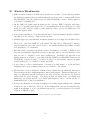
D Performance on Test Models
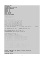
D.1 Experimental Setup . . . . . . . . . . . . . . . . . . . . . . . . . . . . . . . .
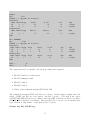
D.2 Data Sets . . . . . . . . . . . . . . . . . . . . . . . . . . . . . . . . . . . . .
D.3 Computational Results . . . . . . . . . . . . . . . . . . . . . . . . . . . . . .
66
66
66
66
3
.
.
.
.
.
.
.
.
.
.
.
.
.
.
.
.
.
.
.
.
.
.
.
.
.
.
.
.
.
.
.
.
.
.
.
.
.
.
.
.
.
.
.
.
.
.
.
.
.
.
.
.
.
.
.
.
.
.
.
.
.
.
.
.
.
.
.
.
.
.
.
.
.
.
.
.
.
.
.
.
.
.
.
.
1
Introduction to FortSP
1.1
The Problem
FortSP is a solver for stochastic linear, and stochastic linear mixed integer programs. In such
a problem the decision variables are governed by linear constraints, with a linear expression
for the objective. To a limited extent some decision variables may be of binary or integer
type. Certain data values will be unknown precisely, and only represented by a discrete range
with a probability given for each set of uncertain values. Knowledge of the random values
will become known in a stage-by-stage progression, and in recourse problems there will be
decision variables reserved for each stage which adapt the solution to unfolding events. User
may add a rider to some constraints that they need only hold with a certain probability.
Recourse Problems
A recourse problem is one in which only some decision variables must be fixed immediately.
Other variables are fixed in stages - those of one period taking into account the scenario
values that have become known in current and in previous stages, but with future stages
still unknown. These postponed decisions are known as recourse variables.
Single Stage
When there are no recourse variables, and all decision variables must be fixed without
knowing the random values, this is then a single-stage model.
Chance and Integrated Chance Constraints
These appear as normal constraints, but whether satisfied or not is subject to the uncertainty.
Chance constraints need only hold with a certain probability in the final solution. Integrated
chance constraints limit the expected violation of the underlying inequalities. The expected
violation can be either expected shorfall or surplus depending on the type of the underlying
constraint. FortSP allows these types of constraints in single and two-stage problems only.
1.2
Data Provision
Information on the model and controls on the execution may be presented on data files
either in SMPS (Stochastic MPS) form, or in SAMPL (Stochastic AMPL) form. These
methods involve use of the stand-alone version of FortSP. It is also possible to use FortSP as
a callable library with entries at which the data is passed internally using SIR (Stochastic
Internal Representation).
SMPS Format
FortSP uses a subset of SMPS (Birge et al., 1987), which is the original standard for stochastic
data provision. In this method three separate data-files are provided:
• Core file: a generic presentation of the variables and constraints in MPS (MPSX)
layout. Data values need not feature any particular scenario, but every random data
element must be represented.
• Time file: Specifying the subdivisions of the core file that belong to each stage.
4
• Stoch file: specifying every scenario, the values of random data, and probabilities. The
layout of stoch-file data lines corresponds to that of the core file. Only discrete forms
of random distributions are considered.
SAMPL Format
AMPL is an algebraic modelling language for mathematical programming problems without
any random component. SAMPL (Valente et al., 2009) is an extension of AMPL able to
specify stochastic components in the appropriate staging. It allows to represent SP problems
using syntax similar to the algebraic notation which is more economical and intelligible
compared to SMPS. Unlike SMPS the whole problem can be specified in one file or divided
into several files according to user requirements. Solver options can be also specified in the
input files, as well as commands to generate an output report from the solution.
FortSP Library Input
When FortSP is used as a subroutine library, input data is entered via subroutine calls over
the argument interface. This interface closely resembles the form of internal data storage,
and may be termed ’Stochastic Internal Representation’. SIR as a file format does not exist
at present, but may be added in future as a medium for saving problem data.
SIR is employed by the SPInE (SP Integrated Environment) system (Valente et al., 2008)
with SAMPL modelling. In SPInE all features of SAMPL are present while FortSP currently
supports a limited subset.
1.3
Solution Methods
A variety of stochastic algorithms are available and these can obtain solutions in one of the
following forms:
• ’Here and Now’ (HN) solution
• ’Wait and See’ (WS) solution
• ’Expected Value’ (EV) solution
HN solution provides the most exact answer to the original SP problem (also the most
difficult) and to solve it there are the following SP algorithms:
• Deterministic Equivalent (DEQ)
• Cutting Plane (CP): either Benders Decomposition for recourse problems, or a special
cutting plane algorithm for single-stage problems with integrated chance constraints
• Stochastic Decomposition (SD), using a random sampling technique. This is limited
to 2-stage recourse problems, with other restrictions to be described later
The following statistical measures may be derived from the solutions of HN, WS and EV
problems:
5
• The expected value of perfect information (EVPI)
• The value of the stochastic solution (VSS).
1.4
External Solvers
Most of the algorithms prepare sub-problems for solution in the form required by the solver
FortMP, which has all the necessary capabilities, but other solvers may also be employed
through the Open Solver Interface (OSI) of the COIN-OR (Lougee-Heimer, 2003) system.
So far the following solvers have been made available:
• FortMP (Ellison et al., 2008), which is the ’natural’ solver
• CPLEX
• CLP
Currently CLP and CPLEX can only be used for solving deterministic equivalent problems.
1.5
Options and Controls
Controls to steer the system by selecting the desired features are to be provided with the
data input. With SAMPL input the option statement can be used to set any option. In the
case of SMPS input either SAMPL script that imports SMPS and set the necessary options
or a separate option file must be provided. The decision between SAMPL script or option
file is made with the command for execution - for example:
fortsp mysp.opt
names the option file to be used by having the extension opt. Any other extension, such
mod in the command
fortsp mysp.mod
invokes the SAMPL translator.
The default input name is fortsp.opt (originally spinesol.opt, but now revised), and
any other name can be specified on the command line that invokes stand-alone FortSP. For
example the command fortsp D:\SPfolder\Myoptions.opt would invoke execution with
data input specified in the named file together with all other controls and options that are
detailed later in this manual.
On this file one control is entered on each line. A list of all options is given in Appendix A.
Each option comprises a keyword followed by a value that is not necessarily numeric. Values
are of the following types:
6
Text
For example, a filename
Switch This is either ON or OFF
Option A keyword
Value
An integer or real numeric value.
Keywords may be given in uppercase or in lowercase, and with or without the underlines
used below purely for spaces in compound keywords.
The format of an option specified by OPT-file is as follows:
<option-keyword> <value>
where the values may be text-strings, switch-settings (ON or OFF), or numeric according
to the specific option. Blank lines may appear anywhere in the opt-file, and comment lines
are indicated by an asterisk (*) in position 1.
In SAMPL it is possible to specify one, two or more options separated by commas in the
same statement. The keyword option is used - the layout being as follows:
option <name> <value>, <name> <value>, ...
;
Option names in SAMPL are closely equivalent to option keywords in an opt-file, but some
differences will appear. Values are either text-strings or numeric, all switches being indicated
with 1 - ON, or 0 - OFF.
An example on the opt-file is as follows:
*
Opt-file option example
MODEL_HN ON
HN_ALGORITHM DETEQI
The same example in SAMPL would be:
# SAMPL option example
option SolveHN 1, SPAlg DetEq;
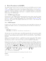
1.6
System Summary
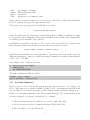
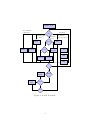
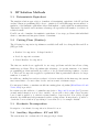
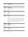
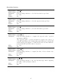
Figure 1 gives a view of the FortSP system from the user perspective. According to the
choice of the inner solver - that is FortMP, CPLEX of CLP - user must have that DLL and
also the DLLs above it in the hierarchy, together with the prime executable fortsp.exe.
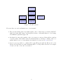
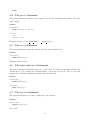
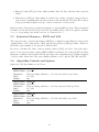
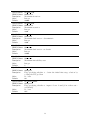
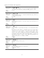
Figure 2 is a simplified summary of the SP algorithm structure. The actual path taken by
execution depends on a variety of indications - for example:
• The model-types chosen for solution (one or more of HN, EV, WS)
• The model-types needed for statistical measures (EVPI and VSS)
• The algorithm to solve the HN model
7
fortsp.exe
FortSP.dll
OsiCpx.dll
OsiFmp.dll
cplex*.dll
FortMP.dll
OsiClp.dll
Figure 1: FortSP system
However there are various limitations to bear in mind
• The special cutting plane algorithm applies only to single-stage problems with ICC.
Other problems with chance and integrated chance constraints must be solved using
deterministic equivalent approach.
• Stochastic decomposition applies only to two-stage recourse problems with no random
objective values, and with no random elements in the second-stage columns of the core
matrix (that is vector c2 and matrix A22 named below in section 2.2, model 2).
• It is not as yet possible to combine SD for the HN model with the EV model or the
WS model (and therefore with calculating EVPI or VSS). Hence the SD box in figure
2 leads out only to the end of execution.
8
SMPS or
SAMPL input
Deterministic
equivalent
Cutting-plane
for ICC
Benders
Level
#Stages
IccCut
2
DetEq
Ancillary
Alg
DetEqX
SD
>2
Nested
Benders
Level?
N
Stochastic
decomposition
EV
Y
WS
Benders
Level
EEV
Compute
EVPI
Compute
VSS
EVPI
VSS
End
Figure 2: FortSP flowchart
9
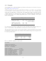
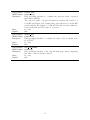
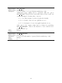
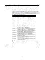
Figure 3: Scenario tree example
2
Mathematical Description of the Problem
Refer to Introduction to Stochastic Programming (Birge and Louveaux, 1997) for a detailed
problem statement and mathematical background.
2.1
Scenario Tree
Stochastic programming can handle large numbers of decision variables and capture their
complex interrelationships stated as constraints in algebraic form. The essence of SP is the
confluence of optimum decision-taking model with the modelling of the random parameter
behaviour. In order to model the behaviour of random parameter values we consider a
limited, discrete sample of the events that may occur between any two stages of the decisiontaking process, and this gives rise to a tree-like branching illustrated in figure 3.
Figure 3 illustrates the scenario tree of a 4-stage decision problem. Each node represents
an optimisation problem for the decisions to be taken there, and the bundle of arcs leading
from the node represents the sampled behaviour in that situation. By scenario is meant
the unfolding of all events (arcs) connecting the current (first) decision (root node) to some
decision in the final stage (leaf node). In general, decision tree analysis can handle only
small data sets, so for realistic problem sizes there is a need for multi-stage SP.
2.2
Two-stage Recourse Models
A two-stage planning horizon is one where immediate (Here and Now) decisions (x1 ) have to
be taken before all the problem elements have become known. Once this happens there are
further, second-stage decisions (x2 ) to be taken according to the newly discovered events.
After splitting the problem into known and unknown (uncertain) elements we have a firststage problem as follows:
10
Minimize
cT1 x1 + θ(x1 )
Subject to g1 ≤ A11 x1
≤ h1
l1 ≤ x1
≤ u1
(1)
where the function θ is the expectation of second-stage utility, given the decisions x1 in the
first stage.
If we select a particular scenario, this utility function will be expressed as follows:
Minimize
cT2 x2
Subject to g2 ≤ A21 x1 + A22 x2 ≤ h2
l2 ≤ x2
≤ u2
(2)
without any further θ-function. Now since x1 is known, the second-stage problem for all
scenarios can be solved, from which we can derive the expectation of utility (probabilityweighted average of the minima), and this defines the θ-function in the first-stage objective.
To express this more exactly we assume the (hypothetical) existence of separate second-stage
decision variables x2s for each scenario s = 1, 2, . . . , S. Couple these with corresponding
values for the uncertain data, and the second-stage model for each scenario becomes:
Minimize
cT2s x2s
Subject to g2s ≤ A21s x1 + A22s x2s ≤ h2s
l2s ≤ x2s
≤ u2s
(3)
So for the expectation we combine the probability-weighted minima of all the second-stage
models, and the entire problem becomes:
Minimize
Subject to g1
g2s
l1
l2s
≤
≤
≤
≤
P
cT1 x1 + Ss=1 ps (cT2s x2s )
A11 x1
A21s x1 + A22s x2s
x1
x2s
≤
≤
≤
≤
h1
h2s , ∀s = 1, . . . , S
u1
u2s , ∀s = 1, . . . , S
(4)
where ps is the probability of scenario s. This formulation of the problem is known as the
Deterministic Equivalent (DEQ).
It was observed in the 50’s that the form (4) is precisely the form solvable with the dual of
Danzig-Wolfe decomposition, also known as Benders’ decomposition or the L-shaped method.
In this method a solution x1 to the model (1) allows dual-solutions of model (3) to be
calculated and applied to form an aggregated ’cut’, which is a constraint added to model (1)
- thus giving a new solution x1 , and so an iterative process is developed. Theory shows that
the iterations converge to precisely the solution of the deterministic equivalent model (4).
It would seem simpler just to solve the DEQ model (4) were it not for the greatly increased
size of the problem. However, the DEQ is useful if the number of scenarios is fairly small.
11
There is a second form of the DEQ that is obtained by postulating separate stage 1 decision
variables for each scenario, and equating them by adding explicit constraints
x1s1 = x1s2
for all pairs of scenarios s1 and s2 (enough pairs to make all scenario-values the same). This
is known as DEQ with Explicit Non-Anticipativity (NA). The original form (4) is known as
DEQ with Implicit NA. For these large problems Interior Point Method (IPM) is usually
chosen in the solution. However, Implicit NA formulation may give difficulty with IPM
owing to column density, and this can be overcome in some cases by using Explicit NA.
2.3
Multi-stage Recourse Models
In a multi-stage (multi-period) planning horizon with more than two stages decisions must
be taken at each stage with knowledge only of the uncertainty in that stage and in previous
stages. We can easily extend the modelling shown in (1) and (3) by considering a θ-function
in all stages except the last. Thus stage 1 is:
Minimize
cT1 x1 + θ1 (x1 )
Subject to g1 ≤ A11 x1
≤ h1
l1 ≤ x1
≤ u1
(5)
The stages are now given by subscript t where t = 1, . . . , T , and so for an intermediate stage
t < T we can say:
Minimize
cTt xt + θt (x1, x2, . . . , xt )
Subject to gt ≤ At1 x1 + At2 x2 + . . . + Att xt ≤ ht
lt ≤ xt
≤ ut
(6)
with variables x1 , x2 , . . . , xt−1 known already. For the last stage we have:
Minimize
cTT xT
Subject to gT ≤ AT 1 x1 + AT 2 x2 + . . . + AT T xT ≤ hT
lT ≤ xT
≤ uT
(7)
with variables x1 , x2, . . . , xT −1 known already. Note that each θ-function depends on the
decisions in that stage and in previous stages, up until the last stage, which has no θfunction. The constraints of the t-th stage involve xt , xt−1 , . . . , x1 (see 1 ).
The solution of such a model requires ’nesting’. A specific model corresponds to a specific
node of the scenario tree (exampled in figure 3). Hence to solve the sub-model for a given
node we need the values of decisions along the path leading up to that node, and all the
solutions to the sub-tree of nodes leading from it. Given a proposed solution for everything
up to stage T − 1, we can adjust the solution of stage T − 1 by applying 2-stage Benders to
each bundle of paths leading from stage T − 1. The same process applies to stage T − 2 by
nesting the last-stage 2-stage Benders inside to form a 3-stage Benders solver. And so on for
1
In a ’Markovian’ situation the t-th stage involves only xt and xt−1 . FortSP handles non-Markovian as
well as Markovian situations
12
the whole tree. Actually the multi-stage Benders algorithm is much faster, using the ’Fast
Forward, Fast Back’ algorithm described in (Birge and Louveaux, 1997) chapter 7.
Solving multi-stage problems with Deterministic Equivalent also involves nesting, and here
the nesting is in the formulation. Consider the (hypothetical) existence of scenario decision
variables for every sub-path on the scenario tree connecting one node to its parent, and
remember that the probability of that path is the sum of the probabilities of all paths leading
through it. Assemble the constraints for all the scenarios and combine in the objective the
sub-path-probability-weighted sum of all scenario objectives (too complicated to express
here in mathematical terminology). This gives the implicit NA version of the DEQ. For the
explicit NA version we consider separate variables for every scenario in every stage, and add
all the constraints needed to equate all the variables for different scenarios that lie along the
same sub-path everywhere in the tree.
2.4
Chance and Integrated Chance Constraints
In addition to multistage recourse problems described above, FortSP supports single and
two-stage problems with individual chance constraints and integrated chance constraints
(ICC). By a singe-stage SP problem we mean the one in which all decisions take place in the
first stage and then the random parameters realise. The difference from a two-stage problem
is that the latter has also a recourse action.
A probabilistic or chance constraint is a constraint that must hold with some minimum probability level. In the framework of model (2) an individual chance constraint corresponding
to i-th row (1 ≤ i ≤ m2 ) can be formulated as:
P{g2i ≤ Ai21 x1 + Ai22 x2 ≤ hi2 } ≥ α,
(8)
where 0 < α < 1 is a reliability level, g2i and hi2 , denote i-th elements of vectors g2 and h2 ;
Ai21 and Ai22 denote i-th rows of matrices A21 and A22 .
The chance constraint constraint (8) has the following deterministic equivalent form:
i
g2s
≤ Ai21s x1 + Ai22s x2s + M vs
Ai21s x1 + Ai22s x2s − M ws ≤ hi2s
vs ≤ zs
ws ≤ zs
S
X
ps zs ≤ 1 − α,
(s = 1, . . . , S)
(s = 1, . . . , S)
(s = 1, . . . , S)
(s = 1, . . . , S)
s=1
where M is a suitably chosen large constant, vs , ws and zs are additional binary variables.
Similarly, below is the formulation of an individual ICC if g2i is infinite for all realisations of
random parameters:
E[(hi2 − Ai21 x1 − Ai22 x2 )− ] ≤ β,
where β ≥ 0 and (a)− := max{−a, 0} is a negative part of a ∈ R.
13
(9)
The ICC (9) has the following deterministic equivalent form:
Ai21s x1 + Ai22s x2s − ws ≤ hi2s (s = 1, . . . , S)
S
X
ps ws ≤ β,
s=1
where ws are additional variables. Note that in the case of integrated chance constraints
introduced variables are continuous which makes deterministic equivalents of ICCs computationally more tractable than those of chance constraints.
If hi2 is infinite for all realisations of random parameters the constraint will look like:
E[(Ai21 x1 + Ai22 x2 − g2i )− ] ≤ β,
The case of both g2i and hi2 finite results in a special case of a joint ICC and is not currently
supported.
14
3
Data Provision in SMPS
3.1
SMPS Input Format
Whereas MPSX defines the format for LP data input, Stochastic MPS (SMPS) defines the
input format for stochastic programming problems. FortSP implements the most important
provisions of SMPS which is described by Birge et al. (1987). Since the solver is initially
designed for use within the SPInE system its stochastic input fulfils the requirements of
models generated by SPInE, and other provisions of SMPS are not supported in full. SPInE
generates solver stochastic data in the form of discrete scenarios, and FortSP supports this
form and also discrete blocks form and discrete independent form.
The stochastic items time-stage, block and scenario are all to be identified by an index with
optional prefix for readability, although SMPS standard calls for identification by the full
name (prefix plus index). FortSP ignores every prefix, but nevertheless user should adopt
the same prefix for the same item throughout, in conformity with the SMPS standard. A
future version of FortSP may be upgraded to identify by name rather than by index.
Three input files are required in order to specify a stochastic problem:
• Core file which is the fundamental problem template in the form of an LP problem
using the MPSX standard
• Time file specifying which rows and columns of the core-file belong to which time stage
• Stoch file specifying the alternative values taken by each random parameter value in
the core file
The user may specify precise names for the input files or may give the basename - or ’Generic’
name - of these files so that extensions are appended automatically. Denoting a base name
by <problem> the resulting filenames are:
<problem>.cor for core file
<problem>.tim for time file
<problem>.sto for stoch file
3.2
Core File and Random Parameter Values
The core file expresses a linear programming problem or linear mixed integer problem in the
format known as MPSX, familiar to the users of LP solvers and described in the manuals
of many of such system, for example, FortMP (Ellison et al., 2008). In this format the file
is divided into ROWS, COLUMNS, RHS, RANGES and BOUNDS sections, and data records have a
fixed format as follows:
Field
Field
Field
Field
Field
Field
1.
2.
3.
4.
5.
6.
Positions
Positions
Positions
Positions
Positions
Positions
2-3 (code)
5-12 (1st name field)
15-26 (2nd name field)
30-37 (1st numeric field)
40-47 (3rd name field)
50-61 (2nd numeric field)
15
This layout is also used for data in the time and stoch files described below.
In the stochastic model a number of scalars will have uncertain values - they are denoted
here as random parameter values. They may be anywhere in the core file other than in the
ROWS section. Each random parameter value must have a representative, finite value assigned
to it in the core model, and this value must be recognisable by the input. It may not be zero
in the COLUMNS or the RANGES section, or left as infinite in the BOUNDS section. However it
does not have to be a value corresponding to any particular scenario.
Both constraints and variables must be grouped according to the stage at which they apply.
These separate groups are to be in the order of time stage in the core file (constraints in
the ROWS section and variables in the COLUMNS section). As a result of this ordering the
constraint matrix should have a lower block triangular form, with blocks for each stage.
MIP in the form of binary or integer descriptions may be applied to any decision variable
(SOS and semi-continuous are not supported). However if it applies to variables other
than the first here-and-now stage then the HN model must be solved using Deterministic
Equivalent methods - Benders’ decomposition would not be suitable.
In the stochastic data (stoch file) the above data-line format is employed without the headers
such as COLUMNS, RHS etc that are used in the core file. For this reason certain names are
reserved as keywords for stochastic data and should not be used either as row or column
names, or as the leading characters of row or column names. These are:
RHS
LHS
RIGHT
LEFT
BOUND
BND
RANGE
RNG
OBJ
COST
Included are any variants of these keywords with lower case lettering. The following are
examples of illegal names:
rhs
Rhside
LeftHS
BOUNDSET objective
bnd1
costrow
RANGEABC
An exception is made for OBJ and COST, which may be used in the name of the actual
objective row (but not in any other row).
3.3
Time File
The time file specifies the first member of each stage grouping in the constraints and variables
of the core model (hence the need to group these items by stage). The first line is as follows:
Positions 1-4
Field 3 (15-22)
Keyword TIME
Problem name
This is followed by the period header line as follows:
Positions 1-7
Field 3 (15-22)
Keyword PERIODS
Keyword IMPLICIT (optional)
After this one line is included for each stage as follows:
16
Field 2 (5-12)
Field 3 (15-22)
Field 5 (40-47)
Starting variable name
Starting constraint name
Stage name
Time stages are indexed 1, 2, . . . with stage number 1 being the first, here-and-now stage.
Finally the data ends with the following line:
Positions 1-6 Keyword ENDATA
The following is an example:
TIME
PERIODS
C1
C6
C8
ENDATA
EXAMPLE
IMPLICIT
R1
R3
R19
STAGE1
STAGE2
STAGE3
Note that in place of R1 it is possible to use the objective row name. The objective row is
moved by the input into the first row position, wherever it is found in the data.
3.4
Stoch File
All random data and the discrete distributions are specified in the stoch file. The first line
is as follows:
Positions 1-5
Field 3 (15-22)
Keyword STOCH
Problem name
This is followed by a header line that specifies the form of data input as follows:
Positions 1 onwards
Field 3 (15-22)
Keyword defining the data form as one of
INDEP BLOCKS SCENARIOS
CHANCE ICC
Keyword DISCRETE
After this header line there are data-lines as described below and the file is terminated as
before:
Positions 1-6 Keyword ENDATA
Sample values for random parameter values are presented in the stoch file in the same form
as they appear in the core file, that is:
Random parameter value in section:
Field
COLUMNS
1:
2:
3:
4:
5:
6:
Column name Vector name
Row name
Row name
Sample value Sample value
2nd row name 2nd row name
Sample value Sample value
2-3
5-12
15-22
25-36
40-47
50-61
RHS
RANGES
17
Vector name
Row name
Sample value
2nd row name
Sample value
BOUNDS
Bound type
Vector name
Column name
Sample value
Fields 5 and 6 have a different use for INDEP-form data (see below), and otherwise can only
be used for random parameter values with the same description in fields 1 and 2.
Any value greater or equal to 1.7×1038 (less or equal to −1.7×1038 ) used as a row or column
bound is treated as a positive (negative) infinity.
Stochastic data form INDEP
INDEP is used when each separate random parameter value has an independent distribution.
Scenarios are built by selecting one possibility for each random parameter value, the set of
all scenarios is then formed by taking all combinations of possible selections.
Each INDEP data line can describe only one random parameter value as follows:
Fields 1-4
Field 5 (40-47)
Field 6 (50-61)
As described above
Stage name
Probability value of the sample (must sum to 1 for each random
parameter value)
Sequence should be according to time stage, and with separate samples of the same random
parameter value collected into consecutive lines. The following is an example:
STOCH
INDEP
C6
C6
C6
C6
C8
C8
C8
ENDATA
EXAMPLE
DISCRETE
OBJ
OBJ
R3
R3
R19
R19
R19
2.5
3.0
5.0
5.5
1.0
2.0
3.0
STAGE2
STAGE2
STAGE2
STAGE2
STAGE3
STAGE3
STAGE3
0.5
0.5
0.33
0.67
0.25
0.25
0.5
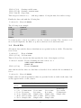
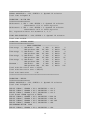
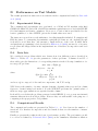
The above example has 12 (2 × 2 × 3) scenarios, illustrated in the following table:
Base
Scen
Scen
1
2
3
4
5
6
7
8
9
10
11
12
core
1
1
1
4
4
1
7
7
7
10
10
Value of
Stage (C6,OBJ)
2
3
3
2
3
3
2
3
3
2
3
3
(C6,R3)
2.5
3.0
-
5.0
5.5
5.0
5.5
18
(C8,R19) Probability
1.0
2.0
3.0
1.0
2.0
3.0
1.0
2.0
3.0
1.0
2.0
3.0
0.04125
0.04125
0.08250
0.08375
0.08375
0.16750
0.04125
0.04125
0.08250
0.08375
0.08375
0.16750
Here the Base Scen column is the scenario containing the default values for any unstated
random parameter values. The first scenario is always based on the core problem and
specifies values for all random parameter values. The Stage column states the stage at
which a difference appears from the base.
Stochastic data form BLOCKS
The nature of this form is very similar to INDEP, except that individual independent random
parameter values give place to independent blocks (or sets) of random parameter values.
The stage number and probability distribution become properties of the block rather than
the individual random parameter value. Each new block and each new set of block values is
introduced with a header line as follows:
Field
Field
Field
Field
1
2
3
4
(2-3)
(5-12)
(15-22)
(25-36)
Keyword BL
Block name
Stage name
Probability value of the sample (must sum to 1 over the samples
of each block)
Blocks with the same name should be grouped together.
Values for the members of each block are entered in a way similar to INDEP data, except
that fields 5 and 6, not being required for stage and probability, may contain a second data
entry for fields 3 and 4 as tabled above in the general stoch file description.
The following is an example:
STOCH
BLOCKS
BL BLOCK1
C6
BL BLOCK1
C6
BL BLOCK2
C8
RHS
BL BLOCK2
C8
RHS
BL BLOCK2
C8
ENDATA
EXAMPLE
DISCRETE
STAGE2
OBJ
STAGE2
OBJ
STAGE3
R19
R19
STAGE3
R19
R19
STAGE3
R19
0.5
2.5
0.5
3.0
0.25
1.0
100.0
0.25
2.0
200.0
0.5
3.0
R3
5.0
R3
5.5
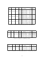
This example gives rise to scenarios in the same manner as before, illustrated as follows:
19
Value of
Scen
Base
Scen
Stage
(C6,OBJ) (C8,R19) Probability
(C6,R3) (RHS,R19)
1
Core
2
2
1
3
2.5
5.0
-
3
2
3
-
4
1
2
5
4
3
3.0
5.5
-
6
5
3
-
1.0
100.0
2.0
200.0
3.0
1.0
100.0
2.0
200.0
3.0
-
0.125
0.125
0.250
0.125
0.125
0.250
Note that block samples do not have to restate values in the block if they duplicate the
previous sample (SMPS standard). Hence the base for samples other than the first of a
block is the previous sample. So in the above example scenarios 3 and 6 assign value 200.0
to (RHS,R19).
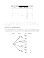
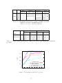
Stochastic data form SCENARIOS
Scenarios have been introduced in the examples above. It may be observed that the branching
of scenarios from each other (i.e. the base scenario connection) forms an event tree in which
decisions may be taken at the nodes. The tree for the INDEP example above looks as follows:
Stage 1
Stage 2
Stage 3
Scenarios
1
2
3
4
5
6
7
8
9
10
11
12
20
In this diagram each scenario is represented by a full path through the nodes from left to
right.
Scenario-form data is prepared from such a tree, which should be known directly or implicitly.
For each scenario it is only necessary to enter the information that differs from its base
scenario - that is the earlier scenario from which it branches. Where several branches issue
from one node (to the right) the later scenarios may be considered as branching from any
earlier scenario in that bundle. Thus for example:
Scenario 10 could branch from 1, 4 or 7
Scenario 6 could branch from 4 or 5
Scenario 1 must always branch from the core model (and provide values for all the random
parameter values).
Each scenario is preceded in the stoch file by a scenario header line as follows:
Field 1 (2-3)
Field 2 (5-12)
Field 3 (15-22)
Keyword SC
Scenario name
Should contain ROOT for scenario 1. For other scenarios enter the
name of the base scenario
Field 4 (25-36) Probability value of the scenario (must sum to 1 over all scenarios)
Field 5 (40-47) Stage index with optional prefix
Data lines for scenarios follow the layout tabled in the general stoch file description.
Here is how the BLOCKS example can be presented in SCENARIOS form:
STOCH
SCENARIOS
SC SCEN1
C6
C8
RHS
SC SCEN2
C8
RHS
SC SCEN3
C8
SC SCEN4
C6
C8
RHS
SC SCEN5
C8
RHS
SC SCEN6
C8
ENDATA
EXAMPLE
DISCRETE
ROOT
OBJ
R19
R19
SCEN1
R19
R19
SCEN2
R19
SCEN1
OBJ
R19
R19
SCEN4
R19
R19
SCEN5
R19
0.125
2.5
1.0
100.0
0.125
2.0
200.0
0.250
3.0
0.125
3.0
1.0
100.0
0.125
2.0
200.0
0.250
3.0
STAGE1
R3
5.0
STAGE3
STAGE3
STAGE2
R3
STAGE3
STAGE3
21
5.5
3.5
Chance and Integrated Chance Constraint Data
Data for chance constraints and ICC are are presented on the STOCH file in additional
sections preceding the random data.
CHANCE section
Chance constraints can be represented in the stoch file using the CHANCE section where the
reliability parameters α are supplied (see section 2.4). The constraints themselves are defined
in the core file and the distributions of their stochastic elements are defined in extra sections
of the stoch file.
After a section header consisting of a single keyword CHANCE in position 1 each line describes
a single chance constraint and has the following structure:
Field
Field
Field
Field
1
2
3
4
(2-3)
L or G denoting constraint sense as in the ROWS section
(5-12) Name of a group of constraint
(15-22) Row name
(25-36) Reliability parameter α, see section 2.4
Example:
CHANCE
G CC1
L CC1
R1
R2
0.95
0.10
The CHANCE section allows one or more groups of chance constraints to be defined. In the
above example, the name of the group is CC1. FortSP uses the first group and ignores all
others.
ICC section
The ICC section is very similar to the CHANCE section. It starts with the keyword ICC followed
by the lines in the form described below:
Field
Field
Field
Field
1
2
3
4
(2-3)
L or G denoting constraint sense as in the ROWS section
(5-12) Name of a group of constraint
(15-22) Row name
(25-36) Parameter β for ICC, see section 2.4
Example:
ICC
L ICC1
R8
10.0
The ICC section allows one or more groups of ICCs to be defined. In the above example, the
name of the group is ICC1. FortSP uses the first group and ignores all others.
22
3.6
Options and Controls for SMPS Data
FortSP gives two possibilities of controling solver execution together with SMPS input. One
is through a separate option file which is described in Section 1.5. Another is through
SAMPL and its SMPS import feature described in Section 4.2.
The following is a table of the options relevant to SMPS input.
Opt-file Name
Description
Value
Default
GENERIC FILENAME
Specifies a stub or generic name for input and output files (i.e. filename without any extension). A standard extension is added for each
actual filename.
String
SPmodel
Opt-file Name
Description
Value
Default
CORE FILE
Actual name of the core file
String
Opt-file Name
Description
Value
Default
TIME FILE
Actual name of the time file
String
Opt-file Name
Description
Value
Default
STOCH FILE
Actual name of the stoch file
String
Opt-file Name
SAMPL Name
Description
Value
Default
OPT DIR
SmpsObjSense
The sense of optimisation for SMPS problems
MIN or MAX
MIN
Opt-file Name
Description
SPS WORKING DIR
Name of the folder to which the current working directory is transferred immediately after input of the option-file has completed, and
before any other input.
All I/O files are located in the local working directory except where a
different path is given with a specific file-name command. Files not so
named take the generic name followed by a standard extension, and
so are located in this directory. In the option-file (not in SAMPL) the
local working directory can be changed by setting this option before
opening any other I/O file.
String
Value
Default
23
4
Data Provision in SAMPL
The primary input format accepted by FortSP when used in the SPInE system is Stochastic
AMPL, or SAMPL, which is described in details in SAMPL/SPInE User Manual (Valente
et al., 2008). SAMPL is an extension of the AMPL modelling language for stochastic programming. It has the advantage of being easier to understand and more compact than
SMPS. As an experimental feature this release of a standalone FortSP solver provides a
limited support for SAMPL input.
4.1
SAMPL Input Format
Current version of the SAMPL translator used in FortSP accepts only two-stage SP problems
expressed in a subset of the language. The syntax can be inferred from the example in
Section 4.9. Details of modelling with SAMPL can be found elsewhere (Valente et al., 2008),
this section only describes the scripting features that can be used to control FortSP and
present the results.
4.2
SMPS Import
FortSP provides a special form of the read statement for importing SMPS problems into the
SAMPL environment. It allows to work with problems in both formats in a uniform way.
Syntax
read-stmt:
read smps ( basename ) ;
read smps ( core-filename, stoch-filename, time-filename ) ;
The first form can be used if the names of the SMPS input files differ only in extension which
is cor for the core file, sto for the stoch file and tim for the time file. The basename is
then their common filename without extension. The second form allows to specify all three
filenames.
SMPS doesn’t specify the direction of optimisation (objective sense) and FortSP assumes
minimisation by default. It can be changed by setting the SmpsObjSense option before
importing the problem. Possible values for this options are Minimize and Maximize.
During the import the name of the SAMPL problem is derived from the SMPS problem name
with all spaces and characters not allowed in SAMPL identifiers replaced with underscores,
e.g. problem-1 is changed to problem 1. The objective name is transformed in the same
way. Two sets called SMPS ROWS and SMPS COLS are introduced which contain the names
of the first-stage rows and columns. SMPS variables and constraints can be accessed using
names smps var and smps con respectively. The variable smps var is indexed over the
set SMPS COLS and the constraint smps con is indexed over SMPS ROWS.
4.3
The solve Statement
The solve statement instantiates the current problem and solves it.
Syntax
solve-stmt:
24
solve ;
4.4
The print Statement
The print statement evaluates each expression in the list and prints the result to the standard output.
Syntax
print-stmt:
print [indexing :] expr-list ;
expr-list:
expr
expr-list , expr
Example: print {c in SMPS COLS}:
4.5
smps var[c];
The write Statement
The write statement writes the current problem in the SMPS form.
Syntax
write-stmt:
write mfilename ;
Example: write mout;
4.6
The model and data Statements
The model and data statements have two forms. The one without arguments switches the
current mode. For example the statement data; enters the data mode. The second form
which takes a filename argument translates the specified file.
Syntax
model-stmt:
model [filename] ;
data-stmt:
data [filename] ;
4.7
The option Statement
The option statement sets and/or prints the option values.
Syntax
option-stmt:
option option-list ;
option-list:
25
option
option-list , option
option:
name [expr]
Here name is an option name and expr is an optional expression of compatible type. If the
expression is not specified the option value is printed. Otherwise the expression is evaluated
and the result is assigned to the option. Example: option Solver OsiClp, LPAlg Dual;
4.8
Built-in Names
SAMPL recognizes the following built-in names.
Name
Description
Infinity The value for representing an infinite bound
evpi
The expected value of perfect information
vss
The value of the stochastic solution
Both evpi and vss apply to the current problem.
In addition to the builtin names the following suffixes are supported.
Suffix
Description
.rc
.body
.ev
.ev rc
.ev body
Reduced cost of a variable
Current value of constraint body
Current value in the EV problem
Reduced cost of a variable in the EV problem
Current value of constraint body in the EV problem
26
4.9
Example
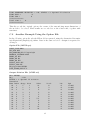
As an example let’s consider the farmer’s problem from Introduction to Stochastic Programming (Birge and Louveaux, 1997).
A European farmer has 500 acres of land where he plans to grow wheat, corn, and sugar
beets. He wants to decide how much land to devote to each crop in order to maximize profit
and produce enough grain to feed his cattle. The farmer knows that at least 200 tons (T)
of wheat and 240 T of corn are needed for cattle feed. All that remains after satisfying the
feeding requirements is sold. Selling and purchase prices as well as planting costs are given
in the following table.
Wheat
Planting cost ($/acre)
Selling price ($/T)
150
170
Purchase price ($/T)
Min. requirement (T)
238
200
Corn
Sugar Beets
230
260
150 36 under 6000 T
10 above 6000 T
210
240
-
Note that sugar beet has two selling prices because the European Commission imposes a
quota on its production. Any amount above the quota is sold at a lower price.
The uncertainty in the problem comes from the weather conditions that affect yields. In this
problem three possible scenarios are considered. The yields in tons per acre are given below
for each crop and scenario.
Wheat
Above
Average
Below
Corn Sugar Beets
2.0
2.5
3.0
2.4
3.0
6.0
Here is a SAMPL formulation of the model:
set Crops;
scenarioset Scenarios;
probability P{Scenarios};
tree Tree := twostage;
param
param
param
param
param
param
param
TotalArea;
Yield{Crops, Scenarios};
PlantingCost{Crops};
SellingPrice{Crops};
ExcessSellingPrice;
PurchasePrice{Crops};
MinRequirement{Crops};
#
#
#
#
#
#
#
acre
T/acre
$/acre
$/T
$/T
$/T
T
27
16.0
200.0
24.0
param BeetsQuota;
# T
# Area in acres devoted to crop c
var area{c in Crops} >= 0;
# Tons of crop c sold (at favourable price in case of beets)
# under scenario s
var sell{c in Crops, s in Scenarios} >= 0, suffix stage 2;
# Tons of sugar beets sold in excess of the quota under
# scenario s
var sellExcess{s in Scenarios} >= 0, suffix stage 2;
# Tons of crop c bought under scenario s
var buy{c in Crops, s in Scenarios} >= 0, suffix stage 2;
maximize profit: sum{s in Scenarios} P[s] * (
ExcessSellingPrice * sellExcess[s] +
sum{c in Crops} (SellingPrice[c] * sell[c, s] PurchasePrice[c] * buy[c, s])) sum{c in Crops} PlantingCost[c] * area[c];
s.t. totalArea: sum {c in Crops} area[c] <= TotalArea;
s.t. requirement{c in Crops, s in Scenarios}:
Yield[c, s] * area[c] - sell[c, s] + buy[c, s]
>= MinRequirement[c];
s.t. quota{s in Scenarios}: sell[’beets’, s] <= BeetsQuota;
s.t. beetsBalance{s in Scenarios}:
sell[’beets’, s] + sellExcess[s]
<= Yield[’beets’, s] * area[’beets’];
The data for the farmer’s problem are as follows:
data;
set Crops := wheat corn beets;
set Scenarios := below average above;
param TotalArea := 500;
param P :=
below
0.333333
average 0.333333
above
0.333333;
28
param Yield:
below average above :=
wheat
2.0
2.5
3.0
corn
2.4
3.0
3.6
beets
16.0
20.0 24.0;
param PlantingCost :=
wheat 150
corn 230
beets 260;
param SellingPrice :=
wheat 170
corn 150
beets 36;
param ExcessSellingPrice := 10;
param PurchasePrice :=
wheat 238
corn 210
beets 100; # Set to a high value to simplify the objective
param MinRequirement :=
wheat 200
corn 240
beets
0;
param BeetsQuota := 6000;
Finally the script file needs to be provided which loads model and data files, solves the
problem and retrieves the optimal value and solution. Due to the flexibility of the AMPL
language SAMPL is based on, it is possible to combine model, data and script in one file
which can be convenient in some cases. However, in general it is not recommended since it
makes more difficult to use the same model with different data sets.
Let’s assume that the model and data are stored in the files farmer.mod and farmer.dat.
The following script loads these files, solves the problem, computes EVPI and VSS and prints
the results:
# Read the model and data.
model farmer.mod;
data farmer.dat;
# Set the options.
option ComputeEvpi 1, ComputeVss 1, VssFStage 1;
# Instantiate and solve the problem.
solve;
29
# Print the results.
print ’Optimal value =’, profit;
print ’EVPI =’, evpi;
print ’VSS =’, vss;
print;
print ’First-stage solution:’;
print {c in Crops}: ’area[’, c, ’] =’, area[c], ’\
’;
print ’totalArea =’, totalArea.body;
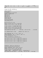
Running FortSP with the command fortsp <script filename> will produce the following
output:
Optimal solution found
Optimal value = 108389.5654
EVPI = 7015.64583
VSS = 1149.8943
First-stage solution:
area[ wheat ] = 170
area[ corn ] = 80
area[ beets ] = 250
totalArea = 500
30
5
SP Solution Methods
5.1
Deterministic Equivalent
The simplest solution approach is to formulate a deterministic equivalent of the SP problem
and use a linear programming (LP) solver to optimise it. FortSP fully supports automatic formulation of deterministic equivalents either with implicit or with explicit non-anticipativity.
This method is feasible and sometimes advantageous especially if the number of scenarios is
relatively small.
FortSP can also formulate deterministic equivalents of two-stage problems with individual
chance constraints and integrated chance constraints.
5.2
Cutting Plane (Benders)
The following decomposition algorithms are available in FortSP for solving the Here-and-Now
(HN) problem:
• Benders’ decomposition - L-shaped method
• Level decomposition variant
• Nested Benders’ decomposition
The first two methods are applicable for two-stage problems and the last allows solving
multi-stage problems. These algorithms take advantage of a specific structure of stochastic
programming problems and make it possible to solve problems with large number of scenarios. The level decomposition applies a regularisation that is particularly effective for larger
numbers of scenarios.
In addition to finding here-and-now values for decision variables in the first stage the system
may extend this to recourse values for the various scenarios in future stages.
For integrated chance constraints an efficient cutting-plane algorithm (Klein Haneveld and
Vlerk, 2002) is provided.
In certain cases the addition of optimality cuts (refer to Birge and Louveaux (1997)) creates
an unbounded situation as θ is a free variable. As an ad-hoc fix for this a large negative
lower bound is applied to θ, which is retained until no longer needed. If not large enough
then the algorithm may halt prematurely with a cycling status. It may then be possible to
obtain the correct solution by specifying a lower value for θ, for example -100000.
5.3
Stochastic Decomposition
Description of stochastic decomposition is deferred for now.
5.4
Ancillary Algorithms - EV and WS
The system may also evaluate the following special problems:
31
• Expected value (EV) problem, which assumes that all data will take their expected
values.
• Wait-and-see (WS) problem, which is obtained by solving a separate sub-problem for
each scenario assuming that all random data is already known. The final WS solution
is the probability-weighted average of these solutions for each scenario.
Each special problem can be evaluated in addition to the main HN problem. When statistical
measures are invoked the EV and/or the WS algorithms will be called as required, whether
or no a corresponding option has been set. see next section 5.5.
5.5
Statistical Measures - EVPI and VSS
The expected value of perfect information (EVPI) is computed as the difference between the
optimal values of the wait-and-see (WS) and the here-and-now (HN) problems. Therefore
the EVPI option implies both options for HN and WS.
In order to calculate the value of the stochastic solution (VSS), we need to know the expectation of the expected value solution (EEV). EEV is calculated by solving the EV problem,
fixing the obtained solution in the WS sub-problems, and computing the probability weighted
objective value. Hence the VSS option implies all three solver options: HN, EV and WS.
5.6
Algorithm Controls and Options
Options for SP algorithms are as follows:
Opt-file Name
SAMPL Name
Description
Value
Default
MODEL HN
SolveHN
Flag specifying whether to solve the here-and-now problem
Boolean
ON
Opt-file Name
SAMPL Name
Description
Value
Default
MODEL EV
SolveEV
Flag specifying whether to solve the expected value problem
Boolean
OFF
Opt-file Name
SAMPL Name
Description
Value
Default
MODEL WS
SolveWS
Flag specifying whether to solve the wait-and-see problem
Boolean
OFF
32
Opt-file Name
SAMPL Name
Description
Value
Default
Opt-file Name
SAMPL Name
Description
Value
Default
Opt-file Name
SAMPL Name
Description
Value
Default
OUTPUT EVPI
ComputeEvpi
Flag specifying whether to compute the expected value of perfect
information (EVPI)
The expected value of perfect information requires the solution of
both HN and WS models. Setting this control ON forces both the HN
switch and the WS switch to be ON. EVPI is the absolute difference
between the HN and WS solution objectives.
Boolean
OFF
OUTPUT VSS
ComputeVss
Flag specifying whether to compute the value of the stochastic solution (VSS)2
Boolean
OFF
VSS FIX FSTAGE
VssFStage
Flag specifying whether to fix only the first stage when computing
the value of the stochastic solution2
Boolean
OFF
33
Opt-file Name
SAMPL Name
Description
Value
HN ALGORITHM
SPAlg
Stochastic programming algorithm to be used
The possible values for this option are listed in the table below.
Opt-file
Name
SAMPL
Name
Description
The algorithm is chosen automatically
(default)
DETEQI
DetEq
The deterministic equivalent problem
with implicit non-anticipativity is constructed and solved
DETEQE
DetEqX
The deterministic equivalent problem with explicit non-anticipativity
constraints is constructed and solved
BENDERS Benders Benders’ decomposition
Level
Variant of level decomposition
STDCMP
Stochastic decomposition
Auto
Default
The default algorithm - Auto - chosen by the system - is Benders’
decomposition for all recourse problems and deterministic equivalent
with implicit nonanticipativity for problems containing chance constraints and integrated chance constraints. An exception to this is
single-stage ICC problems, which by default are solved with the special cutting plane algorithm. All other CC and ICC problems are
solved only with deterministic equivalent, and any specification for
Benders’ or stochastic decomposition is ignored.
Auto
Opt-file Name
SAMPL Name
Description
Value
Default
MAX TIME
MaxTime
Time limit in seconds
Nonnegative number
3600
Options for Benders’ decomposition:
2
VSS - Value of Stochastic Solution - requires the solution of both HN and EV models. Setting this
control ON forces both the HN switch and the EV switch to be ON. In order to calculate VSS we need to know
the EEV - Expected value of the Expected Value solution. EEV is calculated by solving the EV model,
fixing the result so obtained in all the WS models (all stages but the last), which are then solved to give a
probability-weighted average value for the objective - which is the VSS. Option VSS FIX FSTAGE can be used
to restrict the fix that is performed to first stage variables only (although in theory this is not correct, the
theoretical result is often meaningless as a complete fix may be infeasible).
34
Opt-file Name
Description
Value
Default
Opt-file Name
SAMPL Name
Description
Value
Default
Opt-file Name
SAMPL Name
Description
Value
Default
Opt-file Name
SAMPL Name
Description
BEN LEVEL DECOMP
Flag specifying whether to use level decomposition. In SAMPL level
decomposition is enabled by setting the SPAlg option to Level.
0 or 1
1
BEN PREPROC EXP
BenPPExpVal
Flag specifying whether to obtain the initial first stage solution by
solving the EV problem
Boolean
ON
BEN FFFB
BenFffb
Flag specifying whether to use fast forward, fast back method for
multi-stage
Boolean
OFF
Value
Default
BEN THLOB
BenThetaLB
Lower bound for θ used when necessary to avoid unbounded situations.
In certain cases the addition of optimality cuts creates an unbounded
situation as θ is a free variable. As an ad-hoc fix for this, a large
negative lower bound is applied to θ, which is retained until no longer
needed. If not large enough then the Benders algorithm may halt
prematurely with a final condition Cycling (status 6 or larger). It
may then be possible to obtain a correct solution by specifying a lower
value for this option, for example −100000.
Number
-10000
Opt-file Name
SAMPL Name
Description
Value
Default
BEN CUT FACTOR
BenCutFactor
Maximum cuts per child scenario
Integer
20
Opt-file Name
SAMPL Name
Description
Value
Default
BEN MAX ITER
BenMaxIter
Iteration limit for Benders’ decomposition
Nonnegative integer
10000
Options for stochastic decomposition:
35
Opt-file Name
SAMPL Name
Description
Value
Default
SD MAX ITER
SDMaxIter
Maximum iterations
Integer
10000
Opt-file Name
SAMPL Name
Description
Value
Default
SD MAX SCEN
SDMaxScen
Maximum scenarios
Integer
1000
Opt-file Name
SAMPL Name
Description
Value
Default
SD MAX DVD
SDMaxDvd
Maximum dual vertex - deterministic
Integer
1000
Opt-file Name
SAMPL Name
Description
Value
Default
SD MAX DVS
SDMaxDvs
Maximum dual vertex - stochastic
Integer
10000
Opt-file Name
SAMPL Name
Description
Value
Default
SD MAX INFEZ
SDMaxInf
Maximum infeasibility cuts
Integer
5
Opt-file Name
SAMPL Name
Description
SD EXP VAL
SDExpVal
Flag specifying whether to obtain the initial first stage solution by
solving the EV problem
Boolean
ON
Value
Default
Opt-file Name
SAMPL Name
Description
Value
Default
SD INPUT LOBND
SDInputLo
Flag specifying whether to input θ lower bound (if not then autocalculated)
Boolean
OFF
36
Opt-file Name
SAMPL Name
Description
Value
Default
SD LOBND
SDLoBnd
Lower bound for θ
In the SD algorithm a probable lower bound is calculated when
SD INPUT LOBND is OFF. If SD INPUT LOBND is ON, or if the calculation fails, then SD THLOB may supply the missing value.
Number
37
FortSP
DetEq
DetEqX
Benders
OsiCpx
primal
dual
ipm
OsiClp
primal
dual
OsiFmp
primal
dual
Level
LinDamp
SD
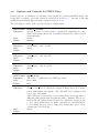
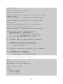
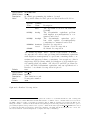
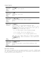
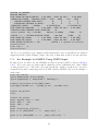
Figure 4: FortSP Algorithms and Solvers
6
Solver Options
6.1
Solvers Available
FortSP has a powerful plug-in system that allows to connect it to different LP solvers through
the COIN-OR (Lougee-Heimer, 2003) Open Solver Interface. On the Windows platform
a plug-in is a dynamically linked library (DLL) that provides access to a single solver.
Currently there are 3 plug-in DLLs: OsiClp.dll for CLP, OsiCpx.dll for CPLEX and
OsiFmp.dll for FortMP. The current solver plug-in can be selected using the Solver option
which takes on the plug-in filename with optional extension as a value.
Figure 4 illustrates which combinations of algorithms and plug-ins are supported in FortSP.
Compatible modules are connected by arcs so, for example, it is possible to solve deterministic
equivalent problems with any solver and LP algorithm while for Benders’ decomposition only
FortMP is currently supported.
6.2
Solver Options and Controls
Options for LP or QP solver execution are as follows:
Opt-file Name
SAMPL Name
Description
Value
Default
Solver
Solver plug-in filename
String
OsiFmp
38
Opt-file Name
SAMPL Name
Description
Value
DEQ ALGORITHM
LPAlg
This option specifies which LP algorithm should be used to solve
a deterministic equivalent problem and all linear programming subproblems that are constructed in the course of solving the SP problem. When using the option-file, option DEQ ALGORITHM applies only
to deterministic equivalent, while USE IPM applies more generally.
The possible values for this option are listed in the table below.
Opt-file SAMPL
Name
Name
Description
Auto
SSX
IPM
Primal
Dual
Ipm
The algorithm is chosen automatically
(default)
Primal simplex method
Dual simplex method
Interior point method
Default
Auto
Opt-file Name
Description
Value
Default
USE IPM
Flag specifying whether to use interior-point method
Boolean
OFF
Opt-file Name
SAMPL Name
Description
Value
Default
BASIS RESTART
WarmStart
Flag specifying whether to use warm start
Boolean
ON
Opt-file Name
Description
Value
Default
SOLVER CPLEX
Flag specifying whether to use CPLEX
Boolean
OFF
39
Opt-file Name
SAMPL Name
Description
USE FORTMP SPECS
UseFortMPSpecs
Flag specifying whether to use extra SPECS-command file (only with
the FortMP solver.)
A SPECS command file with the name fortmp.spc may be used to
refine the options when FortMP is the solver in use. See the FortMP
manual (Ellison et al., 2008). Commands are to be provided in sections corresponding to the type of sub-problem that is being solved,
according to the following table:
Section ID Description
ALL
Value
Default
Section that applies to every call to the solver.
Must appear first in the SPECS file.
DeqImna
Section to handle Deterministic Equivalent Implicit NA
DeqExna
Section to handle Deterministic Equivalent Explicit NA
ExpVal
Section to handle Expected Value solutions
Wsprob
Section to handle Wait and See scenario subproblems
BendRoot Section to handle Benders root-node subproblem solutions (multi-stage)
BendNode Section to handle Benders node sub-problem
solutions other that root or leaf (multi-stage)
BendLeaf Section to handle Benders leaf sub-problem solutions with no warm restart (multi-stage)
BenRLeaf Section to handle Benders leaf sub-problem solutions with warm restart (multi-stage)
Ben2Mast Section to handle Benders master-problem solutions (two-stage)
Ben2Sprb Section to handle Benders sub-problem solutions (two-stage)
LevelQP
Section to handle Benders Level-method QP
solutions (two-stage)
The section ID is named in a BEGIN line - e.g. BEGIN (DeqImna) which is followed by the SPECS commands for that section. Each
section is terminated with a line END.
Boolean
OFF
On the option-file the solver is named in the keyword - to be ON or OFF - while in SAMPL the
corresponding name of the plug-in DLL is to be named. Default in either case is FortMP,
whose plug-in name is OsiFmp. Other possibilities are OsiCpx for CPLEX and OsiClp for
CLP. In the former case CPLEX DLL has to be available.
40
7
Output Files and Logging
Filename for the output file makes use of the generic name (or basename) unless specifically
given by the OUTPUT FILE option. The form of default output filename is as follows
<basename>.sol
7.1
Output and Log Filenames
Outputs from the system comprise two files as follows
• Solution-file:- Giving the model-type solutions that are requested with status and values for both primal and dual solutions. This is limited by default to values for the first
stage only, extendable to further stages by option.
• Log-file:- Giving the outline of processing carried out and diagnostics of any unusual
events or errors occurring.
Filename for these files make use of the ’generic’ name (or basename), as in the case of
default input files. With this name referred to as <model> the output filenames are:
• <model>.sol
• <model>.log
In SAMPL the logging is turned off by default. It can be turned on by setting the LogFile
option.
7.2
Output Controls and Options
Options for solution output and logging are as follows:
Opt-file Name
Description
Value
Default
OUTPUT FILE
Actual name of the output file
String
Opt-file Name
SAMPL Name
Description
Value
Default
LOG FILE
LogFile
Actual name of the log file
String
Opt-file Name
SAMPL Name
Description
Value
Default
LAST STAGE OUTPUT
LastStageOutput
Last stage for which scenario values are required
Integer
1
41
Opt-file Name
SAMPL Name
Description
BEN LOG PRINT
BenLogPrint
Code for items to be logged (Benders multi-stage only)
Additional logged output can be generated with the option
BEN LOG PRINT. This should be used with caution as the log-file can
easily be swamped. Certain values of use are:
• 3 - for solution status of each node (plus the default)
• 19 - for details of the node tree (plus the above)
• 95 - for description of every cut applied (plus the above)
Value
Default
with option 3 the output volume may be reduced by specifying
BEN LOG FREQUENCY - that is the interval to leave between node
solution-status logs.
Integer
1
Opt-file Name
SAMPL Name
Description
Value
Default
BEN LOG FREQUENCY
BenLogFreq
Logged every this number of passes (Benders multi-stage only)
Integer
1
42
References
Ariyawansa, K. A. and Felt, A. J. (2004). On a new collection of stochastic linear programming test problems. INFORMS Journal on Computing, 16(3):291–299.
Birge, J. R., Dempster, M. A. H., Gassmann, H. I., Gunn, E. A., King, A. J., and Wallace,
S. W. (1987). A standard input format for multiperiod stochastic linear programs. COAL
Newsletter, 17:1–19.
Birge, J. R. and Louveaux, F. V. (1997). Introduction to Stochastic Programming. SpringerVerlag, New York.
Consigli, G. and Dempster, M. A. H. (1998). Dynamic stochastic programming for assetliability management. Annals of Operations Research, 81:131–162.
Dolan, E. D. and Moré, J. J. (2002). Benchmarking optimization software with performance
profiles. Mathematical Programming, 91(2):201–213.
Ellison, E. F. D., Hajian, M., Jones, H., Levkovitz, R., Maros, I., Mitra, G., and Sayers,
D. (2008). FortMP Manual. Brunel University: London, Numerical Algorithms Group:
Oxford. http://www.optirisk-systems.com/manuals/FortmpManual.pdf.
Holmes, D. (1995). A (PO)rtable (S)tochastic programming (T)est (S)et (POSTS). http:
//users.iems.northwestern.edu/∼jrbirge/html/dholmes/post.html.
Kall, P. and Mayer, J. (1998). On testing SLP codes with SLP-IOR. In Giannessi,
F., Rapcsák, T., and Komlósi, S., editors, New Trends in Mathematical Programming:
Homage to Steven Vajda, pages 115–135. Kluwer Academic Publishers.
Klein Haneveld, W. K. and Vlerk, M. H. (2002). Integrated chance constraints: reduced
forms and an algorithm. Technical report, University of Groningen, Research Institute
SOM (Systems, Organisations and Management).
König, D., Suhl, L., and Koberstein, A. (2007). Optimierung des Gasbezugs im liberalisierten
Gasmarkt unter Berücksichtigung von Röhren- und Untertagespeichern. In Sammelband
zur VDI Tagung ”Optimierung in der Energiewirtschaft” in Leverkusen.
Lougee-Heimer, R. (2003). The Common Optimization INterface for Operations Research.
IBM Journal of Research and Development, 47(1):57–66.
Valente, C., Mitra, G., Sadki, M., and Fourer, R. (2009). Extending algebraic modelling
languages for stochastic programming. Informs Journal on Computing, 21(1):107–122.
Valente, P., Mitra, G., Poojari, C., Ellison, E. F., Di Domenica, N., Mendi, M., and
Valente, C. (2008). SAMPL/SPInE User Manual. OptiRisk Systems. http://www.
optirisk-systems.com/manuals/SpineAmplManual.pdf.
Zverovich, V., Fábián, C. I., Ellison, F., and Mitra, G. (2009). A computational study of a
solver system for processing two-stage stochastic linear programming problems. Working
paper, CARISMA, Brunel University.
43
APPENDICES
A
Option and Control Summary
A.1
Principle Options and Controls
The following is a complete table of controls and options. References to the notes that follow
the table are given in parenthesis.
Smps Input Options
Opt-file Name
Description
Value
Default
GENERIC FILENAME
Specifies a stub or generic name for input and output files (i.e. filename without any extension). A standard extension is added for each
actual filename.
String
SPmodel
Opt-file Name
Description
Value
Default
CORE FILE
Actual name of the core file
String
Opt-file Name
Description
Value
Default
TIME FILE
Actual name of the time file
String
Opt-file Name
Description
Value
Default
STOCH FILE
Actual name of the stoch file
String
Opt-file Name
SAMPL Name
Description
Value
Default
OPT DIR
SmpsObjSense
The sense of optimisation for SMPS problems
MIN or MAX
MIN
Opt-file Name
Description
SPS WORKING DIR
Name of the folder to which the current working directory is transferred immediately after input of the option-file has completed, and
before any other input.
All I/O files are located in the local working directory except where a
different path is given with a specific file-name command. Files not so
named take the generic name followed by a standard extension, and
so are located in this directory. In the option-file (not in SAMPL) the
local working directory can be changed by setting this option before
opening any other I/O file.
String
Value
Default
44
Algorithm Options
Opt-file Name
SAMPL Name
Description
Value
Default
MODEL HN
SolveHN
Flag specifying whether to solve the here-and-now problem
Boolean
ON
Opt-file Name
SAMPL Name
Description
Value
Default
MODEL EV
SolveEV
Flag specifying whether to solve the expected value problem
Boolean
OFF
Opt-file Name
SAMPL Name
Description
Value
Default
MODEL WS
SolveWS
Flag specifying whether to solve the wait-and-see problem
Boolean
OFF
Opt-file Name
SAMPL Name
Description
OUTPUT EVPI
ComputeEvpi
Flag specifying whether to compute the expected value of perfect
information (EVPI)
The expected value of perfect information requires the solution of
both HN and WS models. Setting this control ON forces both the HN
switch and the WS switch to be ON. EVPI is the absolute difference
between the HN and WS solution objectives.
Boolean
OFF
Value
Default
Opt-file Name
SAMPL Name
Description
Value
Default
Opt-file Name
SAMPL Name
Description
Value
Default
OUTPUT VSS
ComputeVss
Flag specifying whether to compute the value of the stochastic solution (VSS)3
Boolean
OFF
VSS FIX FSTAGE
VssFStage
Flag specifying whether to fix only the first stage when computing
the value of the stochastic solution3
Boolean
OFF
45
Opt-file Name
SAMPL Name
Description
Value
HN ALGORITHM
SPAlg
Stochastic programming algorithm to be used
The possible values for this option are listed in the table below.
Opt-file
Name
SAMPL
Name
Description
The algorithm is chosen automatically
(default)
DETEQI
DetEq
The deterministic equivalent problem
with implicit non-anticipativity is constructed and solved
DETEQE
DetEqX
The deterministic equivalent problem with explicit non-anticipativity
constraints is constructed and solved
BENDERS Benders Benders’ decomposition
Level
Variant of level decomposition
STDCMP
Stochastic decomposition
Auto
Default
The default algorithm - Auto - chosen by the system - is Benders’
decomposition for all recourse problems and deterministic equivalent
with implicit nonanticipativity for problems containing chance constraints and integrated chance constraints. An exception to this is
single-stage ICC problems, which by default are solved with the special cutting plane algorithm. All other CC and ICC problems are
solved only with deterministic equivalent, and any specification for
Benders’ or stochastic decomposition is ignored.
Auto
Opt-file Name
SAMPL Name
Description
Value
Default
MAX TIME
MaxTime
Time limit in seconds
Nonnegative number
3600
3
VSS - Value of Stochastic Solution - requires the solution of both HN and EV models. Setting this
control ON forces both the HN switch and the EV switch to be ON. In order to calculate VSS we need to know
the EEV - Expected value of the Expected Value solution. EEV is calculated by solving the EV model,
fixing the result so obtained in all the WS models (all stages but the last), which are then solved to give a
probability-weighted average value for the objective - which is the VSS. Option VSS FIX FSTAGE can be used
to restrict the fix that is performed to first stage variables only (although in theory this is not correct, the
theoretical result is often meaningless as a complete fix may be infeasible).
46
Options for Benders’ Decomposition
Opt-file Name
Description
Value
Default
Opt-file Name
SAMPL Name
Description
Value
Default
Opt-file Name
SAMPL Name
Description
Value
Default
Opt-file Name
SAMPL Name
Description
BEN LEVEL DECOMP
Flag specifying whether to use level decomposition. In SAMPL level
decomposition is enabled by setting the SPAlg option to Level.
0 or 1
1
BEN PREPROC EXP
BenPPExpVal
Flag specifying whether to obtain the initial first stage solution by
solving the EV problem
Boolean
ON
BEN FFFB
BenFffb
Flag specifying whether to use fast forward, fast back method for
multi-stage
Boolean
OFF
Value
Default
BEN THLOB
BenThetaLB
Lower bound for θ used when necessary to avoid unbounded situations.
In certain cases the addition of optimality cuts creates an unbounded
situation as θ is a free variable. As an ad-hoc fix for this, a large
negative lower bound is applied to θ, which is retained until no longer
needed. If not large enough then the Benders algorithm may halt
prematurely with a final condition Cycling (status 6 or larger). It
may then be possible to obtain a correct solution by specifying a lower
value for this option, for example −100000.
Number
-10000
Opt-file Name
SAMPL Name
Description
Value
Default
BEN CUT FACTOR
BenCutFactor
Maximum cuts per child scenario
Integer
20
Opt-file Name
SAMPL Name
Description
Value
Default
BEN MAX ITER
BenMaxIter
Iteration limit for Benders’ decomposition
Nonnegative integer
10000
47
Options for Stochastic Decomposition
Opt-file Name
SAMPL Name
Description
Value
Default
SD MAX ITER
SDMaxIter
Maximum iterations
Integer
10000
Opt-file Name
SAMPL Name
Description
Value
Default
SD MAX SCEN
SDMaxScen
Maximum scenarios
Integer
1000
Opt-file Name
SAMPL Name
Description
Value
Default
SD MAX DVD
SDMaxDvd
Maximum dual vertex - deterministic
Integer
1000
Opt-file Name
SAMPL Name
Description
Value
Default
SD MAX DVS
SDMaxDvs
Maximum dual vertex - stochastic
Integer
10000
Opt-file Name
SAMPL Name
Description
Value
Default
SD MAX INFEZ
SDMaxInf
Maximum infeasibility cuts
Integer
5
Opt-file Name
SAMPL Name
Description
SD EXP VAL
SDExpVal
Flag specifying whether to obtain the initial first stage solution by
solving the EV problem
Boolean
ON
Value
Default
Opt-file Name
SAMPL Name
Description
Value
Default
SD INPUT LOBND
SDInputLo
Flag specifying whether to input θ lower bound (if not then autocalculated)
Boolean
OFF
48
Opt-file Name
SAMPL Name
Description
Value
Default
SD LOBND
SDLoBnd
Lower bound for θ
In the SD algorithm a probable lower bound is calculated when
SD INPUT LOBND is OFF. If SD INPUT LOBND is ON, or if the calculation fails, then SD THLOB may supply the missing value.
Number
49
Solver Options
Opt-file Name
SAMPL Name
Description
Value
Default
Opt-file Name
SAMPL Name
Description
Value
Solver
Solver plug-in filename
String
OsiFmp
DEQ ALGORITHM
LPAlg
This option specifies which LP algorithm should be used to solve
a deterministic equivalent problem and all linear programming subproblems that are constructed in the course of solving the SP problem. When using the option-file, option DEQ ALGORITHM applies only
to deterministic equivalent, while USE IPM applies more generally.
The possible values for this option are listed in the table below.
Opt-file SAMPL
Name
Name
Description
Auto
SSX
IPM
Primal
Dual
Ipm
The algorithm is chosen automatically
(default)
Primal simplex method
Dual simplex method
Interior point method
Default
Auto
Opt-file Name
Description
Value
Default
USE IPM
Flag specifying whether to use interior-point method
Boolean
OFF
Opt-file Name
SAMPL Name
Description
Value
Default
BASIS RESTART
WarmStart
Flag specifying whether to use warm start
Boolean
ON
Opt-file Name
Description
Value
Default
SOLVER CPLEX
Flag specifying whether to use CPLEX
Boolean
OFF
50
Opt-file Name
SAMPL Name
Description
USE FORTMP SPECS
UseFortMPSpecs
Flag specifying whether to use extra SPECS-command file (only with
the FortMP solver.)
A SPECS command file with the name fortmp.spc may be used to
refine the options when FortMP is the solver in use. See the FortMP
manual (Ellison et al., 2008). Commands are to be provided in sections corresponding to the type of sub-problem that is being solved,
according to the following table:
Section ID Description
ALL
Value
Default
Section that applies to every call to the solver.
Must appear first in the SPECS file.
DeqImna
Section to handle Deterministic Equivalent Implicit NA
DeqExna
Section to handle Deterministic Equivalent Explicit NA
ExpVal
Section to handle Expected Value solutions
Wsprob
Section to handle Wait and See scenario subproblems
BendRoot Section to handle Benders root-node subproblem solutions (multi-stage)
BendNode Section to handle Benders node sub-problem
solutions other that root or leaf (multi-stage)
BendLeaf Section to handle Benders leaf sub-problem solutions with no warm restart (multi-stage)
BenRLeaf Section to handle Benders leaf sub-problem solutions with warm restart (multi-stage)
Ben2Mast Section to handle Benders master-problem solutions (two-stage)
Ben2Sprb Section to handle Benders sub-problem solutions (two-stage)
LevelQP
Section to handle Benders Level-method QP
solutions (two-stage)
The section ID is named in a BEGIN line - e.g. BEGIN (DeqImna) which is followed by the SPECS commands for that section. Each
section is terminated with a line END.
Boolean
OFF
51
Output Options
Opt-file Name
Description
Value
Default
OUTPUT FILE
Actual name of the output file
String
Opt-file Name
SAMPL Name
Description
Value
Default
LOG FILE
LogFile
Actual name of the log file
String
Opt-file Name
SAMPL Name
Description
Value
Default
LAST STAGE OUTPUT
LastStageOutput
Last stage for which scenario values are required
Integer
1
Opt-file Name
SAMPL Name
Description
BEN LOG PRINT
BenLogPrint
Code for items to be logged (Benders multi-stage only)
Additional logged output can be generated with the option
BEN LOG PRINT. This should be used with caution as the log-file can
easily be swamped. Certain values of use are:
• 3 - for solution status of each node (plus the default)
• 19 - for details of the node tree (plus the above)
• 95 - for description of every cut applied (plus the above)
Value
Default
with option 3 the output volume may be reduced by specifying
BEN LOG FREQUENCY - that is the interval to leave between node
solution-status logs.
Integer
1
Opt-file Name
SAMPL Name
Description
Value
Default
BEN LOG FREQUENCY
BenLogFreq
Logged every this number of passes (Benders multi-stage only)
Integer
1
Execution command
The execution command may have an argument naming the option file or SAMPL script
file - fully qualified by the path if different from the current path. By default this file is
fortsp.opt in the current working directory.
52
Keyword and Name Format
On the option file both keywords and text-type values are not case-sensitive. Underline
separators may be omitted, and in three-part keywords only the first letter of the third part
is significant. In SAMPL the option names and text-type values are case-sensitive and must
be given exactly.
Many controls are simple switches that have values ON or OFF in the option file. In SAMPL
these controls have values 0 signalling OFF and 1 signalling ON.
A.2
Miscellaneous commands
A number of additional commands are available that are designed mainly for research purposes. There are also aliases provided to allow for existing usages of the system. A description
will be given here in forthcoming versions of this manual.
53
B
Known Weaknesses
1. SMPS fortmat as used by FortSP relies on indices for scenario- block- and stage-names.
An alphabetic prefix is allowed, which makes the great majority of existing SMPS datafiles intelligible, but the prefix is ignored when identifying a name. Indices must be
consecutive, beginning at 1.
2. On the SMPS Stoch-file random values for the objective, RHS, bound-set and rangeset are to be specified with keywords 4 . Consequently these keywords may not be used
in the Core-file, and the actual core-file names for these objects are unknown to the
Stoch-file input routine.
3. A free-form capability for Core files that allows 15-character numeric fields is available,
but this does not extend to Time and Stoch files.
4. SAMPL support is experimental and many features are not supported in this release.
5. There is no option in SAMPL for Stochastic Decomposition. This method must be
specified with an option file, and does not so far permit ancillary algorithms or statistical measures to be calculated.
6. Execution time is heavily dependent on the total number of scenarios. If this is very
large the deterministic equivalent solvers become impossible to use and Benders’ solver
may become too lengthy for the user’s satisfaction. Stochastic decomposition can
handle many more scenarios, especially with the INDEP and BLOCKS forms for the
STOCH file, but the accuracy of solution is subject to uncertainty, and the stopping
criteria still need to be verified for many problems.
7. A procedure to select a useful subset of scenarios by importance or by Monte-Carlo
sampling has been programmed but is not yet tested to any extent.
8. The Benders’ solver is designed for Markovian stochastic data in which the interaction
between stages in the constraint matrix forms a stair pattern. This means that any one
stage is constrained directly by the previous stage decisions only and not by decisions
earlier than the previous stage. Two-stage models are Markovian. Non-Markovian
multi-stage models should also be solvable with Benders, but, to our knowledge, no
mathematical proof has been published.
9. In rare cases Benders’ solver may be halted by a cycling status with the true optimum
solution not yet reached (see the note on the BenThetaLB option). Cycling may also
result from attempt to solve a non-Markovian model, or from degeneracy if a feasible
solution is difficult to find.
4
The core-file objective name can also be used for random objective values.
54
C
C.1
Examples of Use
An Example Using the Option File
The following is a simple example of a 4-stage model:
Core File (MYSP.cor)
NAME
ROWS
N Z
G R1
G R2
G R3
L R4
G R5
G R6
L R7
G R8
G R9
L R10
COLUMNS
X1
X1
X2
Y1
Y1
Y1
Y2
Y2
Y2
Y3
Y3
RHS
RHS1
RHS1
RHS1
ENDATA
MYSP
(MIN)
Z
R2
Z
Z
R3
R5
Z
R6
R8
Z
R9
3.0
1.0
2.0
-15.0
1.0
2.0
-12.0
1.0
3.0
-4.0
1.0
R3
R6
R9
3.2
3.2
1.0
R1
1.0
R1
R2
R4
1.0
-3.0
1.0
R5
R7
-1.0
1.0
R8
R10
-1.0
1.0
R4
R7
R10
4.0
7.0
1.0
Time File (MYSP.tim)
TIME
PERIODS
X1
Y1
Y2
Y3
ENDATA
MYSP
R1
R2
R5
R8
STAGE001
STAGE002
STAGE003
STAGE004
55
Stoch File (MYSP.sto)
STOCH
SCENARIOS
SC SCEN0001
RHS
RHS
RHS
RHS
RHS
RHS
SC SCEN0002
RHS
RHS
SC SCEN0003
RHS
RHS
RHS
RHS
SC SCEN0004
RHS
RHS
SC SCEN0005
RHS
RHS
RHS
RHS
RHS
RHS
SC SCEN0006
RHS
RHS
SC SCEN0007
RHS
RHS
RHS
RHS
SC SCEN0008
RHS
RHS
ENDATA
MYSP
DISCRETE
ROOT
R3
R4
R6
R7
R9
R10
SCEN0001
R9
R10
SCEN0001
R6
R7
R9
R10
SCEN0003
R9
R10
SCEN0001
R3
R4
R6
R7
R9
R10
SCEN0005
R9
R10
SCEN0005
R6
R7
R9
R10
SCEN0007
R9
R10
0.125
3.2
4.0
3.2
7.0
4.0
8.0
0.125
3.0
6.0
0.125
4.8
9.0
9
12.0
0.125
6.4
18.0
0.125
1.2
4.0
2.2
7.5
3.0
6.0
0.125
4.0
9.0
0.125
2.8
6.0
5.2
12.0
0.125
4.4
8.0
STAGE001
STAGE004
STAGE003
STAGE004
STAGE002
STAGE004
STAGE003
STAGE004
Option File (MYSP.opt)
The following option file causes all forms of output to be generated:
INPUT_TYPE SMPS
OPT_DIR MIN
SPS_WORKING_DIR E:\spine\QA
GENERIC_FILENAME MYSP
56
MODEL_EV ON
MODEL_HN ON
MODEL_WS ON
OUTPUT_EVPI ON
OUTPUT_VSS ON
HN_algorithm BENDERS
BEN_FFFB ON
BEN_PREPROC_EXPVAL ON
VSS_FIX_FSTAGE ON
The run may be started with MYSP.opt named as the argument, or with the above file
actually named as fortsp.opt.
Output Solution File (MYSP.sol)
Outputs from the run are as follows:
WS
WS Scenario = 1
Obj
-140, Prob = 0.125
STATUS = 3: Optimal LP solution
Variables
Name Index Stage
Value
X1
1
1
12
X2
2
1
0
Constraints
Name Index Stage
SPrice
R1
2
1
0
END
WS Scenario = 2
Obj
-132, Prob = 0.125
STATUS = 3: Optimal LP solution
Variables
Name Index Stage
Value
X1
1
1
12
X2
2
1
0
Constraints
Name Index Stage
SPrice
R1
2
1
0
END
D.val
0
2
Lob
0
0
Upb
1e+035
1e+035
RowAct
12
Lhs
0
Rhs
1e+035
D.val
0
2
Lob
0
0
Upb
1e+035
1e+035
RowAct
12
Lhs
0
Rhs
1e+035
. . . .
Etc, repeated as above for scenarios 3, 4, 8
. . . .
WS Summary
Obj
-149
STATUS = 3: Optimal LP solution
END
57
ExpVal
Obj
-152
STATUS = 3: Optimal LP solution
Variables
Name Index Stage
Value
X1
1
1
12
X2
2
1
0
Constraints
Name Index Stage
SPrice
R1
2
1
0
END
D.val
0
2
Lob
0
0
Upb
1e+035
1e+035
RowAct
12
Lhs
0
Rhs
1e+035
HN = BENDERS
Obj
-149
STATUS = 3: Optimal LP solution
Variables
Name Index Stage Scen
Value
X1
1
1
1
12
X2
2
1
1
0
Constraints
Name Index Stage Scen
Value
R1
2
1
1
12
END
EVPI =
VSS =
D.val
0
2
Lob
0
0
Upb
1e+035
1e+035
D.val
0
Lhs
0
Rhs
1e+035
0
0
The output shown above includes only 1st stage values and comprises:
• The WS solution for each scenario
• The WS summary result
• The EV solution
• The HN solution
• Values of the statistical measures EVPI and VSS
The statistical measures EVPI and VSS are both zero in this simple example since the
values of EEV and WS are both equal to the HN objective. Note that if the option
VSS FIX FSTAGE ON had been omitted, then the EEV would in fact have been infeasible and VSS would have been infinite. Theoretically V SS = 0 is not correct but this value
is probably more important to a user than V SS = inf inity.
Output Log File (MYSP.log)
58
INPUT_TYPE SMPS
OPT_DIR MIN
SPS_WORKING_DIR E:\spine\QA
GENERIC_FILENAME MYSP
MODEL_EV ON
MODEL_HN ON
MODEL_WS ON
OUTPUT_EVPI ON
OUTPUT_VSS ON
HN_algorithm BENDERS
BEN_FFFB ON
BEN_PREPROC_EXPVAL ON
VSS_FIX_FSTAGE ON
Specification file read
Current Working directory: E:\spine\QA
FORTMP release version 3.02g, Aug 2002
License expires on (y)2010:(m)01:(d)01.
License expires on (y)2010:(m)01:(d)01.
FORTMP release version 3.02g, Aug 2002
License expires on (y)2010:(m)01:(d)01.
TIME TAKEN FOR INPUT MPS
=
0.00 SECS,
**** PROBLEM NAME IS: MYSP
TOTAL SO FAR =
, GENERIC FILE: MYSP ****
CORE DIMENSIONS: NR= 11, NC = 5, NNZ = 19
STOCH DIMENSIONS:- ANT = 4, ANS = 8, AND = 28
Stoch representation code :1
Number of Scenarios to process = 8
======================================
Time period 1 has 1 rows 2 columns and 2 nonzeroes
Time period 2 has 3 rows 3 columns and 4 nonzeroes
Time period 3 has 3 rows 2 columns and 4 nonzeroes
Time period 4 has 3 rows 2 columns and 4 nonzeroes
===========================================
ALGORITHM:- WAIT & SEE
**********************
WS Scenario 1, OBJ = -140, STATUS = 3: Optimal LP solution
Contributes -17.5 to final objective
WS Scenario 2, OBJ = -132, STATUS = 3: Optimal LP solution
Contributes -16.5 to final objective
Etc, repeated as above for scenarios 3, 4, 8
. . . .
FINAL WS OBJECTIVE = -149, STATUS = 3: Optimal LP solution
Total time in WS:0
ALGORITHM:- EXPVAL
59
0.00 SECS
**********************
EXPVAL OBJECTIVE = -152, STATUS = 3: Optimal LP solution
Total time in ExpVal:0
ALGORITHM:- WS FOR EEV
**********************
WS Scenario 1, OBJ = -140, STATUS = 3: Optimal LP solution
Contributes -17.5 to final objective
WS Scenario 2, OBJ = -132, STATUS = 3: Optimal LP solution
Contributes -16.5 to final objective
Etc, repeated as above for scenarios 3, 4, 8
. . . .
FINAL EEV OBJECTIVE = -149, STATUS = 3: Optimal LP solution
Total time in WS:0
ALGORITHM:- BENDERS DECOMP
**************************
------------------ NODE DIMENSIONS -----------------Time-stage
1, Sub-model:
NR=
1, NC=
2, NAIJ=
Sub-problem: NR=
44, NC=
3, NAIJ=
Time-stage
2, Sub-model:
NR=
3, NC=
3, NAIJ=
Sub-problem: NR=
45, NC=
2, NAIJ=
Time-stage
3, Sub-model:
NR=
3, NC=
4, NAIJ=
Sub-problem: NR=
45, NC=
2, NAIJ=
Time-stage
4, Sub-model:
NR=
3, NC=
5, NAIJ=
Sub-problem: NR=
5, NC=
2, NAIJ=
Maximum Sub-model:
NR=
3, NC=
5, NAIJ=
Sub-problem: NR=
45, NC=
3, NAIJ=
Total node Col-vector size = 31(*2)
Total node Row-vector size = 354(*3)
Total node basis size
= 36
=====================================================
ALGORITHM:- EXPVAL
**********************
EXPVAL OBJECTIVE = -152, STATUS = 3: Optimal LP solution
Total time in ExpVal:0
END OF ITER# 1, STAGES 1 TO 4, OBJECTIVE
END OF ITER# 2, STAGES 3 TO 3, OBJECTIVE
END OF ITER# 3, STAGES 2 TO 2, OBJECTIVE
Lower Bound -10000 applied to THETA
END OF ITER# 4, STAGES 1 TO 4, OBJECTIVE
END OF ITER# 5, STAGES 2 TO 2, OBJECTIVE
END OF ITER# 6, STAGES 1 TO 4, OBJECTIVE
END OF ITER# 7, STAGES 1 TO 4, OBJECTIVE
NEW BENDERS OPTION: FFSB
END OF ITER# 8, STAGES 1 TO 4, OBJECTIVE
60
= -112.5
= -112.5
= -112.5
=
=
=
=
2526.59
2526.59
-147.364
-149
= -149
2
125
4
85
4
85
4
5
4
125
FINAL BENDECOMP OBJECTIVE = -149, STATUS = 3: Optimal LP solution
FINAL EVPI =
0
FINAL VSS =
0
===============
Total time =
0
===============
This file records the original options, the events of the run and important dimensions of
the models to be solved. Final results are recorded as on the solution file, together with
run-times.
C.2
Another Example Using the Option File
In the following option file only the HN model is requested, using the alternative Deterministic Equivalent (implicit) algorithm. Data is the same as before. Output is requested for
all stages.
Option File (MYSP.opt)
INPUT_TYPE SMPS
OPT_DIR MIN
SPS_WORKING_DIR E:\spine\QA
GENERIC_FILENAME MYSP
MODEL_EV OFF
MODEL_HN ON
MODEL_WS OFF
OUTPUT_EVPI OFF
OUTPUT_VSS OFF
HN_algorithm DETEQI
LAST_STAGE_OUTPUT 4
Output Solution File (MYSP.sol)
HN = DETEQI
Obj
-149
STATUS = 3: Optimal LP solution
Variables
Name Index Stage Scen
Value
X1
1
1
1
12
X2
2
1
1
0
Y1
3
2
1
4
Y1
3
2
5
4
Y2
4
3
1
7
Y2
4
3
3
8
Y2
4
3
5
7.5
Y2
4
3
7
6
Y3
5
4
1
8
Y3
5
4
2
6
Y3
5
4
3
12
Y3
5
4
4
18
D.val
0
2
0
0
0
0
0
0
0
0
0
0
61
Lob
0
0
0
0
0
0
0
0
0
0
0
0
Upb
1e+035
1e+035
1e+035
1e+035
1e+035
1e+035
1e+035
1e+035
1e+035
1e+035
1e+035
1e+035
Y3
Y3
Y3
Y3
5
5
5
5
4
4
4
4
Constraints
Name Index Stage
R1
2
1
R2
3
2
R3
4
2
R4
5
2
R2
3
2
R3
4
2
R4
5
2
R5
6
3
R6
7
3
R7
8
3
R5
6
3
R6
7
3
R7
8
3
R5
6
3
R6
7
3
R7
8
3
R5
6
3
R6
7
3
R7
8
3
R8
9
4
R9
10
4
R10 11
4
R8
9
4
R9
10
4
R10 11
4
R8
9
4
R9
10
4
R10 11
4
R8
9
4
R9
10
4
R10 11
4
R8
9
4
R9
10
4
R10 11
4
R8
9
4
R9
10
4
R10 11
4
R8
9
4
R9
10
4
R10 11
4
R8
9
4
5
6
7
8
6
9
12
8
0
0
0
0
Scen
1
1
1
1
5
5
5
1
1
1
3
3
3
5
5
5
7
7
7
1
1
1
2
2
2
3
3
3
4
4
4
5
5
5
6
6
6
7
7
7
8
Value
12
0
4
4
0
4
4
1
7
7
0
8
8
0.5
7.5
7.5
2
6
6
13
8
8
15
6
6
12
12
12
6
18
18
16.5
6
6
13.5
9
9
6
12
12
10
D.val
0
-3
0
4.5
0
0
7.5
0
0
3
-3
0
0
0
0
3
0
0
3
0
0
0.5
0
0
0.5
0
0
0.5
0
0
0.5
0
0
0.5
0
0
0.5
0
0
0.5
0
62
0
0
0
0
Lhs
0
0
3.2
-1e+035
0
1.2
-1e+035
0
3.2
-1e+035
0
4.8
-1e+035
0
2.2
-1e+035
0
2.8
-1e+035
0
4
-1e+035
0
3
-1e+035
0
9
-1e+035
0
6.4
-1e+035
0
3
-1e+035
0
4
-1e+035
0
5.2
-1e+035
0
1e+035
1e+035
1e+035
1e+035
Rhs
1e+035
1e+035
1e+035
4
1e+035
1e+035
4
1e+035
1e+035
7
1e+035
1e+035
9
1e+035
1e+035
7.5
1e+035
1e+035
6
1e+035
1e+035
8
1e+035
1e+035
6
1e+035
1e+035
12
1e+035
1e+035
18
1e+035
1e+035
6
1e+035
1e+035
9
1e+035
1e+035
12
1e+035
R9
R10
END
10
11
4
4
8
8
8
8
0
0.5
4.4
-1e+035
1e+035
8
Output Log File (MYSP.log)
INPUT_TYPE SMPS
OPT_DIR MIN
SPS_WORKING_DIR E:\spine\QA
GENERIC_FILENAME MYSP
MODEL_EV OFF
MODEL_HN ON
MODEL_WS OFF
OUTPUT_EVPI OFF
OUTPUT_VSS OFF
HN_algorithm DETEQI
LAST_STAGE_OUTPUT 4
Specification file read
Current Working directory: E:\spine\QA
FORTMP release version 3.02g, Aug 2002
License expires on (y)2010:(m)01:(d)01.
License expires on (y)2010:(m)01:(d)01.
FORTMP release version 3.02g, Aug 2002
License expires on (y)2010:(m)01:(d)01.
TIME TAKEN FOR INPUT MPS
=
0.00 SECS,
**** PROBLEM NAME IS: MYSP
TOTAL SO FAR =
0.00 SECS
, GENERIC FILE: MYSP ****
CORE DIMENSIONS: NR= 11, NC = 5, NNZ = 19
STOCH DIMENSIONS:- ANT = 4, ANS = 8, AND = 28
Stoch representation code :1
Number of Scenarios to process = 8
======================================
Time period 1 has 1 rows 2 columns and 2 nonzeroes
Time period 2 has 3 rows 3 columns and 4 nonzeroes
Time period 3 has 3 rows 2 columns and 4 nonzeroes
Time period 4 has 3 rows 2 columns and 4 nonzeroes
===========================================
ALGORITHM:- DETEQ with IMPLICIT NA
**********************************
DETEQI DIMENSIONS: NR=43, NC=16, NAIJ=58
FORTMP release version 3.02g, Aug 2002
License expires on (y)2010:(m)01:(d)01.
ASGNFM: MREQ=
220952(Byte), OFFset=
10223672(Byte)
TIME TAKEN FOR INPUT/SETUP =
0.00 SECS, TOTAL SO FAR =
63
0.00 SECS
SCALING IN PROGRESS ...
SCALING COMPLETE
TIME TAKEN FOR SCALE/PRSLVE=
0.00 SECS, TOTAL SO FAR =
0.00 SECS
CRASH(LTSF) ENDED. VARIABLE TYPES:- PLUS
BNDD
FIX
FREE
LOGICALS REMOVED FROM BASIS:16
0
0
0
STRUCTURALS ENTERED IN BASIS:16
0
0
0
CRASH(ART) ENDED:
1 PASSES:
0 ARTIFICIALS,
0 PIVOTED OUT
TIME TAKEN FOR CRASHING
=
0.00 SECS, TOTAL SO FAR =
0.00 SECS
FEASIBLE BASIS REACHED AFTER ITERATION
10
Invert demand: Obj =-149.000
Suminf = 0.00000
ITER#
22
STATUS = 3 -- OPTIMUM SOLUTION FOUND.
-149.000
ITER#
22
TIME TAKEN FOR PRIMAL
=
0.00 SECS, TOTAL SO FAR =
0.00 SECS
TIME TAKEN FOR OUTPUT
=
0.00 SECS, TOTAL SO FAR =
0.00 SECS
FINAL DETEQI OBJECTIVE = -149
, STATUS = 3: Optimal LP solution
===============
Total time =
0
===============
The above log includes logged output from the internal LP solver for the HN model, which is
suppressed in the earlier example owing to the large volume that would be shown otherwise.
C.3
An Example in SAMPL Using SMPS Input
In this section we will solve the STORM problem from the POSTS collection (Holmes,
1995). It is a two-stage problem with stochasticity in the right-hand side. Since SMPS
doesn’t specify how to control the solver and present the output you will need to provide a
script file in another format supported by FortSP which is SAMPL. Below is an example of
such script:
# Set the options.
option SPAlg DetEq, Solver OsiClp;
option ComputeEvpi 1, ComputeVss 1, VssFStage 1;
# Import the problem in the SMPS format.
read smps(’stormG2.cor’, ’stormG2_27.sto’, ’stormG2.tim’);
# Solve the problem.
solve;
# Print the results.
print ’Optimal value =’, OBJ;
print ’EVPI =’, evpi;
print ’VSS =’, vss;
print;
print ’First-stage solution:’;
print {c in _SMPS_COLS}: c, ’=’, _smps_var[c], ’\
’;
print {r in _SMPS_ROWS}: r, ’=’, _smps_con[r].body, ’\
’;
64
Note that the SP algorithm is set to DetEq which means that the deterministic equivalent
will be constructed and solved using the current solver. In this example we set the solver to
OsiClp. The deterministic equivalent approach doesn’t scale well with increasing problem
dimensions and the number of scenarios as shown in Appendix D. Therefore, for solving larger
instances of the STORM problem as well as other problems level or Benders’ decomposition
is recommended.
Running FortSP with the command fortsp <script filename> will produce the following
output:
Optimal solution found
Optimal value = 15508982.31
EVPI = 32422.97538
VSS = 6004.125768
First-stage solution:
C0011901 = 0
C0012001 = 0
C0012101 = 0
C0012201 = 0
C0012301 = 0
C0012401 = 0
C0012501 = 0
C0012601 = 0
C0012701 = 0.66
C0012801 = 3.34
and 300 more lines...
65
D
Performance on Test Models
The results presented in this section are taken from the computational study by Zverovich
et al. (2009).
D.1
Experimental Setup
The computational experiments were performed on a Windows XP machine with Intel
CORE2 2.4 GHz CPU and 3 GB of RAM. Deterministic equivalents were solved with CPLEX
11.0 dual simplex and barrier optimisers. Crossover to a basic solution was disabled for the
barrier optimiser, for other CPLEX options the default values were used.
The times are reported in seconds with times of reading input files included. For simplex and
IPM the times of constructing deterministic equivalent problems are also included though
it should be noted that they only amount to small fractions of the total. FortMP linear
and quadratic programming solver described by Ellison et al. (2008) was used to solve master problem and subproblems in the implementations of Benders decomposition and level
method.
D.2
Data Sets
We considered test problems which were drawn from four different sources described in
Table 13. Tables 14 – 18 give the parameters of these problems. Columns A and W of
these tables give the dimensions of corresponding matrices in the following formulation of a
two-stage SP problem:
min cT x + EQ(x, ξ)
subject to Ax = b,
x ≥ 0,
where
Q(x, ξ) = min q T y
subject to W y = h − T x,
y≥0
and vector ξ is composed of the random components of h, T, W and q.
NNZ denotes the number of nonzero matrix elements. Optimal values reported in column
Opt were obtained using level method. For the WATSON problems the optimal values of
their two-stage approximations are specified in this column.
It should be noted that the problems generated with GENSLP do not possess any internal
structure inherent in real-world problems. However they are still useful for the purposes of
comparing scale-up properties of algorithms.
D.3
Computational Results
The computational results are presented in Tables 19 – 23. Iter denotes the number of
iterations. For Benders decomposition and level method these are the numbers of master
iterations.
Finally we present the results in the form of performance profiles. The performance profile
for a solver is defined by Dolan and Moré (2002) as the cumulative distribution function
66
Source
1. POSTS collection
Reference
Comments
Holmes (1995)
Two-stage problems from the test set
called POSTS
2. Slptestset collection Ariyawansa and Felt
(2004)
Two-stage problems from the collection
of stochastic LP test problems
3. Random problems
Kall and Mayer
(1998)
Artificial test problems generated with
pseudo random stochastic LP problem
generator GENSLP
4. SAMPL problems
König et al. (2007),
Valente et al. (2008)
Instances of the SAPHIR gas portfolio
planning model formulated in SAMPL
5. WATSON problems
Consigli and
Dempster (1998)
WATSON pension fund management
test problems
Table 13: Sources of test problems
Name
A
W
pltexpA2
62×188
104×272
fxm2
92×114
238×343
185×121
528×1259
stormG2
Scen
6
16
6
16
8
27
125
1000
Deterministic Equivalent
Matrix
NNZ
686×1820
3703
1726×4540
9233
1520×2172
12139
3900×5602
31239
4409×10193
27424
14441×34114
90903
66185×157496 418321
528185×1259121 3341696
Opt
-9.47935
-9.66234
18416.8
18416.8
15535236
15508982
15512091
15802590
Table 14: Parameters of test problems from POSTS collection
Name
AIRL2
LandS
A
2×4
2×4
W
6×8
7×12
4node
14×52
74×186
Scen
25
3
16
32
64
128
256
512
1024
2048
4096
8192
16384
32768
Deterministic Equivalent
Matrix
NNZ
152×204
604
23×40
92
1198×3028
7743
2382×6004
15231
4750×11956
30207
9486×23860
60159
18958×47668
120063
37902×95284
239871
75790×190516
479487
151566×380980
958719
303118×761908 1917183
606222×1523764 3834111
1212430×3047476 7667967
2424846×6094900 15335679
Opt
269665
381.853
423.012
423.013
423.012
423.012
425.375
429.962
434.113
441.738
446.856
446.856
446.856
446.856
Table 15: Parameters of test problems from Slptestset collection
67
Name
A
W
rand0
50×100
25×50
rand1
100×200
50×100
rand2
150×300
75×150
Scen
2000
4000
6000
8000
10000
2000
4000
6000
8000
10000
2000
4000
6000
8000
10000
Deterministic Equivalent
Matrix
NNZ
50050×100100
754501
100050×200100 1508501
150050×300100 2262501
200050×400100 3016501
250050×500100 3770501
100100×200200 3006001
200100×400200 6010001
300100×600200 9014001
400100×800200 12018001
500100×1000200 15022001
150150×300300 6758501
300150×600300 13512501
450150×900300 20266501
600150×1200300 27020501
750150×1500300 33774501
Opt
162.146
199.032
140.274
170.318
139.129
244.159
259.346
297.562
262.451
298.638
209.151
218.247
239.720
239.158
231.706
Table 16: Parameters of test problems generated with GENSLP
Name
A
W
saphir
32×53
8678×3924
Scen
50
100
200
500
1000
Deterministic Equivalent
Matrix
NNZ
433932×196253 1136753
867832×392453 2273403
1735632×784853 4546703
4339032×1962053 11366603
8678032×3924053 22733103
Opt
129506233
129059362
141473266
137871740
133036857
Table 17: Parameters of SAMPL problems
Name
WATSON.I
A
W
11×15
324×587
Scen
128
256
512
1024
Deterministic Equivalent
Matrix
NNZ
41483×75151
188828
82955×150287 377628
165899×300559 755228
331787×601103 1510428
Opt
-2271.17866
-2733.63695
-2810.75153
-2750.48955
Table 18: Parameters of two-stage approximations of WATSON problems
68
Name
pltexpA2
fxm2
stormG2
Scen
6
16
6
16
8
27
125
1000
CPLEX
IPM
Simplex
Time Iter
Time
Iter
0.06 14
0.15
329
0.13 16
0.17
810
0.09 17
0.24 1281
0.20 23
0.47 3374
0.38 28
0.32 3675
3.33 27
0.87 13128
12.33 57
7.00 71611
189.53 109 305.81 758078
FortSP
Benders
Level
Time Iter Time Iter
0.04 1
0.03 1
0.08 4
0.10 4
0.29 23
0.35 15
0.39 22
0.53 18
0.60 23
0.83 22
1.93 30
1.65 22
8.38 32
4.99 19
80.20 41 34.46 18
Table 19: Solution times and iteration counts for POSTS problems
for a performance metric. We use the ratio of the solving time versus the best time as the
performance metric. Let P and M be the set of problems and the set of solution methods
respectively. We define by tp,m the time of solving problem p ∈ P with method m ∈ M . For
every pair (p, m) we compute performance ratio
rp,m =
tp,m
,
min{tp,m |m ∈ M }
If method m failed to solve problem p the formula above is not defined. In this case we set
rp,m := ∞.
The cumulative distribution function for the performance ratio is defined as follows:
ρm (τ ) =
|{p ∈ P |rp,m ≤ τ }|
|P |
We calculated performance profile of each considered method on the whole set of test problems. These profiles are shown in Figure 5. The value of ρm (τ ) gives the probability that
method m solves a problem within a ratio τ of the best solver. For example according to
Figure 5 level method was the first in more than 30% of cases and solved all the problems
within a ratio 6 of the best time.
The notable advantages of performance profiles over other approaches to performance comparison are as follows. Firstly, they minimize the influence of a small subset of problems
on the benchmarking process. Secondly, there is no need to discard solver failures. Thirdly,
performance profiles provide a visualisation of large sets of test results as we have in our
case.
Figure 5 illustrates that, while in most cases the performance of CPLEX barrier optimiser
is better it was not able to solve some of the problems. Several large instances were not
solved due to high memory requirements of constructing and solving deterministic equivalent.
Other failures were caused by numerical difficulties. The performance profiles of pure Benders
decomposition and linear damping are very similar to each other and the level method profile
dominates both of them.
69
Name
AIRL2
LandS
4node
IPM
Time Iter
0.04 11
0.04 9
0.19 17
0.65 15
0.70 17
0.71 26
1.53 30
3.38 30
7.51 32
17.93 36
44.95 45
79.73 45
Scen
25
3
16
32
64
128
256
512
1024
2048
4096
8192
16384
32768
CPLEX
Simplex
Time
Iter
0.14
145
0.11
21
0.20 1461
0.37 3244
0.88 6847
2.48 13498
9.88 27743
41.74 54861
457.53 130701
1262.75 239159
11733.86 475971
∗
∗
†
†
†
†
†
†
†
†
FortSP
Benders
Level
Time Iter
Time Iter
0.08 10
0.16 16
0.01 8
0.04 9
1.44 102
1.18 47
3.60 130
1.87 66
6.79 135
2.36 54
10.25 115
3.37 45
16.17 101
8.75 60
34.04 109
18.08 67
69.13 110
36.34 68
240.25 184
63.28 59
538.26 215
129.57 63
1474.48 286
229.72 56
1850.52 194
459.27 58
5785.07 279 1029.74 65
Table 20: Solution times and iteration counts for Slptestset problems
∗
†
‡
Name
rand0
rand1
rand2
Scen
2000
4000
6000
8000
10000
2000
4000
6000
8000
10000
2000
4000
6000
8000
10000
Failed to solve due to timeout
Failed to solve due to insufficient memory
Failed to solve due to numerical difficulties
CPLEX
IPM
Simplex
Time Iter
Time
Iter
16.71 44
541.78 84571
30.11 40 2632.72 155926
56.90 52 8688.20 257614
∗
∗
83.35 57
∗
∗
142.82 79
∗
∗
66.92 24
∗
∗
162.20 29
∗
∗
252.81 30
∗
∗
386.67 35
†
†
∗
∗
164.18 22
∗
∗
†
†
∗
∗
†
†
†
†
†
†
†
†
†
†
†
†
FortSP
Benders
Level
Time Iter
Time Iter
62.68 80
33.73 42
112.91 72
59.41 37
287.09 124
137.20 58
341.97 110
171.42 55
831.67 219
293.24 76
760.06 388
161.81 76
1786.76 496
258.74 69
2010.50 368
316.25 54
3063.53 435
544.61 72
4012.57 451
694.83 70
5821.79 889
427.70 67
3881.73 397
451.03 43
7555.65 522
901.72 51
8678.47 478
883.14 41
15984.27 698 1536.32 60
Table 21: Solution times and iteration counts for generated problems
∗
†
Failed to solve due to timeout
Failed to solve due to insufficient memory
70
Name
saphir
CPLEX
Simplex
Time
Iter
‡
255.03 73918
‡
916.04 143194
‡
7579.14 385231
IPM
Time Iter
Scen
50
100
200
500
1000
‡
‡
‡
†
†
†
†
†
†
†
†
FortSP
Benders
Level
Time Iter
Time Iter
465.18 113
396.59 76
701.14 120
533.06 60
‡
‡
2555.47 206
2556.06 115 2339.76 59
4294.47 109 4650.19 78
Table 22: Solution times and iteration counts for SAMPL problems
†
‡
Name
WATSON.I
Failed to solve due to insufficient memory
Failed to solve due to numerical difficulties
Scen
128
256
512
1024
CPLEX
IPM
Simplex
Time Iter Time Iter
1.71 33
1.44 7985
3.89 38
3.66 15818
8.91 47
5.88 30237
20.27 54 14.44 60941
FortSP
Benders
Level
Time Iter Time Iter
0.92 1
0.92 1
1.58 1
1.59 1
2.62 1
2.61 1
5.12 1
5.31 1
Table 23: Solution times and iteration counts for two-stage approximations of WATSON
problems
1
ρm (τ )
0.8
0.6
0.4
CPLEX Ipm
CPLEX Simplex
FortSP Benders
FortSP Level
FortSP Lin.Damp.
0.2
0
1
2
4
8
16
32
64 128 256 512
τ
Figure 5: Performance profile in a log2 scale
71