Download here - Bedzyk Research Group

4-Circle 18KW User Manual v5
NU X-Ray Lab
M.J. Bedzyk
July 1, 2010
4-Circle User Manual
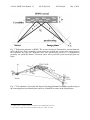
Fig. 1 NU X-ray Lab 4-Circle Diffractometer at end of 18 KW Cu rotating anode beam line.
Fig. 2 Top-view schematic diagram of beamline components. (Not to scale.)
4-Circle 18KW User Manual v5
NU X-Ray Lab
M.J. Bedzyk
July 1, 2010
Beamline Components: (In sequence, starting from source, refer to Fig. 2.)
 18KW Ultrex Rigaku Rotating Anode (donated by Abbott Labs in 2006)
• Cu Anode: Cu Kα1 λ = 1.5406 Å
Cu Kα2 λ =1.54443 Å
• Point Source: Normal Focus 0.5 mm x 10 mm, 18 KW max power
o The effective source size should be 0.5-mm high by 1-mm-wide due to 6° take-off
angle . But we measure the width to be 0.5 mm wide. (See Fig. 3.)
• Nominal operating power: 50 KV, 240 mA
• Huber slits for controlling horizontal and vertical divergence (See Fig. 3.)
o Nominal setting: hsdgap= 0.7 mm wide by 14-mm-high
o 1 full turn of the dial on a Huber slit translates the blade 0.50 mm.
• Graphite (002) Grade ZYA ( < 0.5° mosaic) from Advanced Ceramics Corp.
o Size: 25 x 25 x 2 mm
o Para-focusing in the horizontal direction
o Sagittal-focusing in the vertical direction with Rs = 225 mm
o 2d002 = 6.708 Å, Cu Kα1 θ = 13.28°
o 1 to 1 focusing, F1=F2=F= RS /sinθ = 980 mm. This is the distance from the
source to the mono and from the mono to the sample.
(See Appendix D for ray diagrams illustrating Parafocusing and Sagittal focusing.)
• Incident beam intensity monitor (NaI detector collecting scattered x-rays from Co coated
Kapton foil) I0 = 8900 cps at hsdgap = 0.7 mm and vsdgap = 14 mm.
• Huber incident beam slits for passing Cu Kα1 and blocking Cu Kα2
o Nominal setting ka2cen = 0, ka2gap = 0.5 mm-wide by 1-mm high
• Huber 4-circle diffractometer
o Motorized Z-sample, zsamp = 0 should put pin in COR (Center of Rotation)
o Huber 1006 X-Y-χ−φ goniometer
o Sample holder
o 2-theta arm: (Nominal settings)
 guard slit ( gshhcen = 0.64, gshgap = 1.1, gsvcen = 1.4, gsvgap = 8 )
 XIA filter box, ( T = 0.24 x 0.01 for STB straight thru beam)
(See Appendix A for SPEC Macros for controlling XIA Filter Box.)
 detector slit, ( dshhcen = 0.05, dshgap = 1.0, dsvcen = 1.9, dsvgap = 12 )
 Cyberstar NaI X-ray detector (0.3µsec, 740V, Gain =8, LL=2.5, UL=6.5)
• Auxillary equipment:
o Laser Level on Tripod
o X-ray Eye
o Goniometer pin
o High-power zoom lens camera
Β
Operating Procedures:
1. Introduction: In describing the procedures for operating the 4-circle, we will use as an
example the following MBE grown thin-film sample:
a. 200 Å BaTiO3 / 20 Å SrTiO3 / Si(001) substrate
b. The STO (SrTiO3) fillm will be very difficult to sense because it is so thin.
c. We will study the thicknesses of the layers by low-angle XRR
d. We will determine the miscut angle of the surface relative to the Si(001)
e. We will determine the single crystal quality of the BTO film
4-Circle 18KW User Manual v5
NU X-Ray Lab
M.J. Bedzyk
July 1, 2010
f. We will determine the epitaxial orientation of the BTO film
g. We will determine the out-of-plane and in-plane BTO lattice constants to define
the strain state of the film. i.e., Is the BTO film coherently strained or fully
relaxed or partly strained?
2. Startup Computer at LINUX PC
a. Open 1st Terminal
b. Create your own folder with your name and change to that directory.
i. [user4circle@euler ~]$ mkdir YourDirectoryName
ii. [ ] $ cd YourDirectoryName
c. [ ] $ fourc (This takes you into SPEC)
i. qdo /home/user4circle/macros/prpeak
ii. FOURC> on(“BTO_STO_Si001_b.log”) . This will make a log file of
everything you do in SPEC.
iii. FOURC> startup
1. Answer questions
2. (newfile) All of your scans will be found in this filename you must
give BTO_STO_Si001_b
3. (setlat) Set your sample substrate lattice constants: 5.431
4. (setaz) Set the HKL for the surface normal direction: 0 0 1
d. Open a 2nd Terminal
i. $ cd YourDirectoryName
ii. $ newplot (this program will let you load your SPEC file and plot any of
the scans
3. Power up 18KW generator:
a. Target: ON
b. X-Ray: ON
c. Voltage: Arrow up to 50 KV, SLOWLY
d. Current: Arrow UP to 240 mA, SLOWLY
e. Put all XIA filters IN to protect NaI Cyberstar detector
f. Manually set vertical gap of slit before graphite mono at ~14 mm
g. Manually set vertical gap of incident beam slit before sample at ~1 mm
h. Flip Shutter Switch: UP (Red Warning Light ON at Rotating Anode Head)
4. Diffractometer Alignment Procedures
a. FOURC> an 0 0, > umv chi 90, > umv zsamp -15 Takes 2θ, θ to 0, χ to 90°
b. > umv hsdgap 0.7 , > umv ka2gap 0.5 , > umv gshgap 10 , > umv dshgap 1
c. > umv dsvgap 15 and > umv gsvgap 15 should be nearly wide open so you
integrate in χ direction.
d. XIA Filters: T = 0.24 * 0.01 = 2.4 x10-3 (Top and bottom Filters ON, others OFF)
e. Check to make sure that only the single beam of the Cu Ka1 (and not Ka2) is
transmiting through the incident beam slit (ka2cen ka2gap).
i. Make sure nothing is blocking the beam at the sample position
ii. > dscan tth -.5 .5 40 .5 , > umv tth CEN , > set tth 0, > pplot
4-Circle 18KW User Manual v5
NU X-Ray Lab
M.J. Bedzyk
July 1, 2010
1. You should see one and only one symmetrical peak , otherwise
some Ka2 is coming thru.
2. The peak should be ~13,000 cts per 0.5 sec with FWHM=0.1°
a. This is ~ 3x107 photons per second in the incident beam.
3. If your findings for this scan are significantly below these
expectated values, then you need to solicate expert help from Jerry
Carsello or someone in Bedzyk’s group.
4. Subsequent steps f and g should be skipped unless you think the
incident beam and diffractometer center have been misaligned.
f. Use Long distance Microscope of Zoom Video camera to insure goniometer pin is
in diffractometer rotation center.
i. Manually adjust X & Y of goniometer head until pin XY position is
invarient to φ rotation.
ii. Adjust zsamp, until pin Z position is invarient to χ rotation.
g. Make sure incident beam coincides with diffractometer center by taking a burn at
the pin or by using an X-ray eye to see silhouette (shadow) of pin in beam center.
If the beam is not going through the diffractometer center, solicate expert help
from Jerry Carsello or someone in Bedzyk’s group.
5. Sample Alignment Procedure
a. Mount sample and laser align surface normal with φ axis. Use tripod mounted
Laser Level.
i. Observe laser reflected beam from sample mirror surface at a couple of
meters from sample.
ii. Adjust the 2 arcs of the goniometer head until laser reflected beam
position is invarient to φ rotation.
iii. Adjust χ until the reflected laser beam is at the incident beam height.
1. >set chi 90, now the φ axis is perfectly horizontal.
2. Note that at χ = 0 the φ axis and θ axis are aligned and have the
same right-handed sense of rotation.
b. Align sample surface with incident beam:
i. Adjust zsamp until the sample surface is roughly cutting the beam in half
as observed by the detector counts.
ii. > dscan th -2 2 40 .5, > umv th CEN, > set th 0
iii. > dscan zsamp -1 1 40 .5, > umv zsamp CEN
iv. repeat steps ii and iii, until no further adjustment are needed.
c. Record STB (Straight thru beam condition)
i. > umvr zsamp -2
ii. > prlm (this prints out a wa, wh, and ct)
iii. Make sure to record in your Notebook and in this STB printout, the Filter
setting, e.g., T = 0.24 x 0.01
SHOW ZSAMP SCAN> EXPLAIN HOW BEAM WIDTH CAN BE
DETERMINED> AND HOW BEAM VERTICAL MISALIGNMENT
CAN BE DIAGNOSED.
6. Find the first allowed substrate Bragg peak near the specular rod
4-Circle 18KW User Manual v5
NU X-Ray Lab
M.J. Bedzyk
July 1, 2010
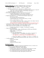
Fig. 3 The Si(004) rocking curve (RC) peak reflected p/s and FWHM dependence on,
hsdgap, the horizontal width of the slit 850 mm from the source and 110 mm before the
monochromator. Over this range the monitor cps are directly proportional to hsdgap. The
fit confirms that the RC FWHM is a direct measure of the incident beam divergence and
that the effective horizontal source size is 0.53 mm.
a. > ca 0 0 4 (gives tth and th for the Si(004) peak base on Braggs’ Law)
b. > an 69.0985 34.5493 (This takes tth and th to the respective values in deg )
c. > dscan th -.2 .2 40 .5, > umv th CEN, record FWHM=0.055°, > pplot
i. Since the Si (004) angular acceptance width (Darwin width) = 3.5 arcsec =
0.001 ° is very small and since the Cu Ka1 wavelength spread Δλ/λ=
2x10-4 is very small, this FWHM is a direct measure of the incident beam
horizontal divergence from the parafocussing Graphite monochromator .
(See Fig. 3) This FWHM corresponds to a transverse ΔQ= QΔω=2π/d Δω
= 0.0044 1/Å at the Si(004).
d. > dscan chi -2 2 40 .5, > umv chi CEN, record FWHM=1.57°, >pplot
i. There should be a small flat top region at the peak of the chi scan so that
you will be integrating in this direction of reciprocal space. If there is no
flat top you need to increase the vertical gap size of the slits on the
detector arm.
e. > d2scan tth -.2 .2 th -.1 .1 40 .5 , umv tth CEN, umv th (look up th in scan
table), record FWHM= 0.097° in tth
i. This corresponds to a longitudinal ΔQ=Qcot(θ) Δθ = 0.0057 1/Å
f. > ct , now reduce filters until ct shows 40kcps < DET < 150kcps
i. for this Si(004) T=0.24 and DET= 99.9kcps
g. Repeat steps c to e until th, chi and tth converge. tth should precisely match
Braggs’ Law for Cu Ka1 and substrate lattice constant.
4-Circle 18KW User Manual v5
NU X-Ray Lab
M.J. Bedzyk
July 1, 2010
h. > or0 0 0 4 (this is for the orientation matrix)
i. > prlm (Paste this in your NoteBook. Label it as Si(004) peak at T=0.24.)
7. Adjusting the vertical divergence: Notice that due to the large vertical gaps in the slits
before the monochromator and on the detector arm, there is a very large ~1° vertical
divergence in the instrument. This comes from the vsdgap=14mm vertical source
divergence gap of the manually adjusted slit in front of the mono. 14mm / 850 mm =
16.5mrad=0.94°. Therefore you want to scan in th and tth, while integrating in the chi
(vertical) direction. Otherwise, what you will see in the scanned peak widths is this large
instrumental broadening. Therefore if you want to do a reciprocal space 2D map, scan in
th at different tth. Or reduce vertical divergence by reducing vsdgap. The flux and
vertical divergence of the incident beam on the sample are proportional to vsdgap, for
2<vsdgap<20. You could also reduce the vertical gaps of the detector and guard slits.
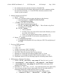
8. Finding small miscut angle of surface relative to
low-index crystal crystal planes.
a. Rotate PHI in 45° steps
b. At each PHI, find the theta center for the Si
004 Bragg peak
c. Make a PHI , Theta table in K-graph
d. Fit this data to Y = A*Sin(X-X0)+ Y0
i. A= Miscut degree angle, We
found 0.35° miscut
ii. X0 = PHI angle that you should go
to so that the plane formed by
surface normal and [001] is
perpendicular to scattering plane.
Also this makes alpha=beta . You
of course can go to PHI+180.
iii. Y0= middle value of omega. Y0
should equal tth/2 = θB.
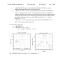
Fig. 4 The Si (004) RC peak θ
position as a function of the
azimuthal angle φ. The fit to the data
determines the miscut angle between
the [004] xtal direction and the
surface normal.
9. Find off-normal low-index substrate Bragg peak.
E.g. Si (202)
a. > ca 2 0 2 This gives 2θ, θ, χ should be ~ 45°, At this point φ is incorrect
b. > an 47.299 23.6495 , > umvr chi -45 (this is the case for moving to the Si (202)
c. > ascan phi 50 140 900 .5 ( this course scan will pass through one of the “4-fold
symmetric” {202} peaks. ) Found 202 peak at φ =133.6°
d. a full 360° phi scan shows all 4 peaks separated in 90° intervals
e. > dscan phi -.1 .1 40 .5 , > umv phi CEN, φ = 133.57°
f. > dscan th -.2 .2 40 .5, > umv th CEN,
g. > dscan chi -2 2 40 .5 , umv chi CEN,
h. > d2scan tth -.2 .2 th -.1 .1 40 .5, umv tth CEN umv th (look up th in scan
table)
i. repeat above e. thru h. centering scans until no change
j. >or1 2 0 2
4-Circle 18KW User Manual v5
NU X-Ray Lab
M.J. Bedzyk
July 1, 2010
k. >prlm (paste this in your NoteBook label it as Si(202) peak and T=0.24.)
l. If you want to do scans in this vicinity of recip space you should do > or_swap
m. > pa ( this will tell you the primay and secondary HKL used for determining the
orientation matrix)
n. You can now describe the 3D crystallographic direction of the miscut. Use Fig. 4
and Step 7e, φ = 133.57° to do this.
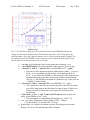
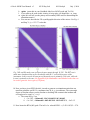
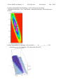
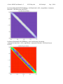
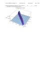
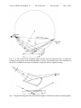
Fig. 5 HL and KL mesh scans (reciprocal space maps) through Si 202 . The HL scan is
much more broadened due to the convolution with the 1° vertical divergence of the
instrument. In this case the H-scan part of the mesh scan is primarily a chi-scan, while the
k-scan is primarily a th-scan. (See Appendix B for Mathematica and MatLab codes that can
be used to generate these types of 2D plots.)
10. Now you have given SPEC the info it needs to generate a orientation matrix that can
transform substrate xtal H K L coordinates into 2θ, θ, χ, φ coordinates. The extra angle
degree of freedom allows you the freedom to do things like constrain the incident and
exit angles to be equal. i.e., α = β.
a. The scans in Fig. 5 are
i. > br 2 0 2, > hklmesh L 1.96 2.04 40 H 1.96 2.04 40 2
ii. > br 2 0 2, > hklmesh K -.005 .005 20 L 1.99 2.015 25 1, >br 2 0 2
11. Now locate the BTO (002) peak. The in Si r.l.u. relaxed BTO L = (5.431/4.03)*2 = 2.70.
4-Circle 18KW User Manual v5
NU X-Ray Lab
M.J. Bedzyk
July 1, 2010
a. > ubr 0 0 2.70, The peak was found at the bulk-like BTO lattice constant
position, indicating that the film was fully relaxed.
b. > d2scan tth -2 2 th -1 1 100 5 This longitudinal scan peak has a FWHM(2θ) =
0.643° =11.2 mrad at 2θ= 44.977°. You can use these values in conjuntion to
compute FWHM(Q) and use this in the 1D interference function to determine the
vertical domain size D001 of the BTO film and compare that to the film thickness
that will be found later in the low-angle XRR measurement. D = 2π/ΔQ =
2π/0.04Å-1 = 157 Å.
c. > dscan th -1.5 1.5 30 1, this transverse scan peak has a th FWHM=0.716° at
22.40°. The in-plane domain size is D|| =
⊥
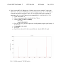
12. Locate BTO (001) peak.
a. > ubr 0 0 1.35
b. > d2scan tth -2 2 th -1 1 50 5
i. D = 2π/ΔQ = 2π/0.04Å-1 = 157 Å
⊥
Fig. 6 The BaTiO3 (001) tth-th scan. Q = 4π sin(2θ/2) / λ .
4-Circle 18KW User Manual v5
NU X-Ray Lab
M.J. Bedzyk
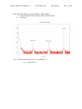
13. 00L Specular Reflecivity scan for BTO / STO/ Si(001).
a. > a2scan tth 0.0765 80.0765 th 0.03825 40.0382 2000 3
b. > See Fig. 7
Fig. 7 00L Specular Reflecivity. Q = 4π sin(2θ/2) / λ .
i. Q = 4π sin(2θ/2) / λ
July 1, 2010
4-Circle 18KW User Manual v5
NU X-Ray Lab
M.J. Bedzyk
July 1, 2010
14. Now locate the BTO 202 Bragg peak. With the cube-on-cube rotated 45° epitaxy the
BTO 202 in Si reciprocal lattice units (r.l.u.) should appear at |H| = |K|=2, if the fillm is
coherently strained to match the Si lattice. If it is relaxed to bulk lattice constants, it
should be at |H| = |K| =1.92. The in Si r.l.u. relaxed BTO L = (5.431/4.03)*2 = 2.70.
a. > ubr 1.92 -1.92 2.70
b. follow centering procedure described in Step 7 above.
c. > for ( i=1.82 ; i<=2.02 ; i+=0.002){
br i -i 2.6
lscan 2.6 2.8 100 1}
d. You can do a 360° phi-scan to prove the 4-fold symmetry single crystal epitaxy of
the thin film.
e. > ascan phi 0 360 3600 .5
f. See Fig. 8.
g. Fig. 9 shows the set of H=-K scans at different L thru the BTO 202 peak.
Fig. 8 “4-fold symmetric” Si{202} peaks.
4-Circle 18KW User Manual v5
NU X-Ray Lab
M.J. Bedzyk
July 1, 2010
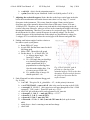
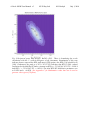
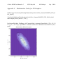
Fig. 9 Reciprocal space map through BaTiO3 (202) . There is broadening due to the
convolution with the 1° vertical divergence of the instrument. Examination of this scan
indicates that as expected the BTO (and unseen STO) epitaxy has BTO [110] parallel to Si
[100]. Futhermore the peak at (1.921,-1.921,2.702) indicates that BTO is fully relaxed
(unstrained) with bulk-like RT lattice constants at BTO a = 2*5.431Å/(1.921*√2) = 3.998 Å
and BTO c = 2*5.431Å/2.702 = 4.020 Å. The ideal BTO RT bulk-lattice parameters are
a=3.992Å and c =4.032Å. (See Appendix C for Mathematica codes that can be used to
generate these types of 2D plots.)
4-Circle 18KW User Manual v5
Appendix A
NU X-Ray Lab
M.J. Bedzyk
July 1, 2010
SPEC Macros for controlling XIA Filter Box
SPEC Macros available for convenient operation
FOURC> prlm ( Sends to X-ray lab printer: ct, wh )
FOURC> pplot (Sends to X-ray lab printer: splot )
FOURC> inifilters (initializes autofilter function)
FOURC> setfilter 1234 (set filter 1,2,3,4 as the current condition to start)
FOURC> insertfil wxyz (insert filters 1,2,3,4 )
For example, insertfil 124 will insert filters 1,2 & 4
FOURC> insert_all (insert all filters)
FOURC> removefil wxyz (removes filters 1,2,3,4 )
Check to see if macros are loaded by issuing the command
e.g. FOURC> inifilter (If SPEC says “Not a command or macro” then you need to load macros
1. Load basic macros
h. At the fourc terminal window
i. FOURC> qdo /home/user4circle/macros/4cstart.mac
(This “4cstart” macros includes all necessary functions like “pplot”, “prlm”.)
2. Load autofilter controlling macros
j. Enable/disable autofilter control by flipping the on/off switch button in the front
panel of XIA filter box in the cart to “ON”.
k. FOURC> qdo /home/user4circle/macros/pfcusave.mac
l. Flip the filter box to NO filter condition by moving all 1,2,3,4 filter switches to
“out” status
m. FOURC> inifilters (this will initialize autofilter macros)
n. FOURC> setfilters 1234 (this will set filter 1,2 3,4 as the current condition to
start)
o. Use commands above to insert or remove filters
p. To go back to manual control mode for the filter box, simply flip the filter box to
“off” status at the front panel.
4-Circle 18KW User Manual v5
Appendix B
NU X-Ray Lab
M.J. Bedzyk
July 1, 2010
Mathematica and MatLab Codes for 2D Graphics
Mathematica Codes
SetDirectory["/Users/bedzyk/Desktop/Data&Analysis/4circle18kw_Summer2008/BTO_STO_Si
001_july08/BTO_STO_Si001_c"]
/Users/bedzyk/Desktop/Data&Analysis/4circle18kw_Summer2008/BTO_STO_Si001_july08/BT
O_STO_Si001_c
Directory[]
/Users/bedzyk/Desktop/Data&Analysis/4circle18kw_Summer2008/BTO_STO_Si001_july08/BT
O_STO_Si001_c
dataKLSi202=Import["s172_KLScanSi202.csv","CSV"];
dataHLSi202=Import["s169_HLScanSi202.csv","CSV"];
ListContourPlot[dataKLSi202,PlotRange->All,FrameLabel->{K,L},AspectRatio->Automatic,
PlotLabel->"KL Mesh Scan at Si(202)"]
4-Circle 18KW User Manual v5
NU X-Ray Lab
M.J. Bedzyk
July 1, 2010
ListDensityPlot[dataKLSi202,PlotRange->All,ColorFunction->Hue,Mesh>Automatic,FrameLabel->{K,L},AspectRatio->Automatic,PlotLabel->"KL Mesh Scan at
Si(202)"]
ListPlot3D[dataKLSi202,PlotRange->All,AxesLabel->{___ _K ___ _,___ L___,_CPS
___},BoxRatios->{1,2.5,1},PlotLabel->"KL Mesh Scan at Si(202)"]
4-Circle 18KW User Manual v5
NU X-Ray Lab
M.J. Bedzyk
July 1, 2010
ListContourPlot[dataHLSi202,PlotRange->All,FrameLabel->{H,L},AspectRatio->Automatic,
PlotLabel->"HL Mesh Scan at Si(202)"]
ListDensityPlot[dataHLSi202,PlotRange->All,ColorFunction->Hue,Mesh>Automatic,FrameLabel->{H,L},AspectRatio->Automatic,PlotLabel->"HL Mesh Scan at
Si(202)"]
4-Circle 18KW User Manual v5
NU X-Ray Lab
M.J. Bedzyk
July 1, 2010
ListPlot3D[dataHLSi202,PlotRange->All,AxesLabel->{___ _H ___ _,___ L___,_Counts
___},PlotLabel->"HL Mesh Scan at Si(202)"]
4-Circle 18KW User Manual v5
NU X-Ray Lab
M.J. Bedzyk
July 1, 2010
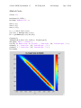
MatLab Codes
clear all
D=zeros(11,1681);
D=load('HLmesh.txt');
X=D(:,1);
Y=D(:,3);
Z=D(:,11);
ti = 1.96:0.001:2.04;
[XI,YI] = meshgrid(ti,ti);
ZI = griddata(X,Y,Z,XI,YI);
figure(1)
imagesc(X,Y,ZI(1:81,1:81)); figure(gcf)
set(gca,'YDir','normal')
title('HL Mesh Scan at Si(202)','fontsize',14,'fontweight','b')
xlabel('H','fontsize',10,'fontweight','b')
ylabel('L','fontsize',10,'fontweight','b')
colorbar
4-Circle 18KW User Manual v5
Appendix C
NU X-Ray Lab
M.J. Bedzyk
July 1, 2010
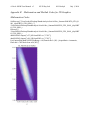
Mathematica Codes for 2D Graphics
SetDirectory["/Users/bedzyk/Desktop/Data&Analysis/4circle18kw_Summer2008/BTO_STO_Si
001_july08"]
/Users/bedzyk/Desktop/Data&Analysis/4circle18kw_Summer2008/BTO_STO_Si001_july08
data1=Import["HLcts_data.csv","CSV"];
ListContourPlot[data1, PlotRange->All,ContourLabels->Automatic,FrameLabel->{"H = -K [ Si
r.l.u.]","L [ Si r.l.u.]"},AspectRatio->Automatic, PlotLabel->"hklmesh scans at BaTiO3 (2 0 2)
peak"]
4-Circle 18KW User Manual v5
Appendix D
NU X-Ray Lab
M.J. Bedzyk
July 1, 2010
Parafocusing and Sagittal focusing
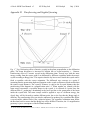
Fig. 1.1 Top: Defocusing effect of mosaic crystals in the plane perpendicular to the diffraction
plane. The beam divergence is increased in 2τSinθB due to crystal mosaicity, τ . Bottom:
Parafocusing effect of a mosaic crystal in the diffraction plane: Several rays with the same
energy coming from the source point S are diffracted by different crystallites inside the mosaic
crystal according to Bragg's law. This requires that the ray has to travel inside the crystal until it
finds a crystallite with the correct orientation. The diffracted rays converge to a point S’
(assuming that the penetration depth and footprint on the crystal are distances much smaller than
the source-crystal distance). The crystal-Sʹ′ distance is equal to the S-crystal distance thus the
parafocusing effect happens in a magnification ratio 1:1. When another ray (dotted) with the
same energy encounters a crystallite deeper in the crystal, it is reflected to a point close but
different from Sʹ′, producing a broadening in the focal spot due to the penetration of the beam
inside the crystal bulk. The same concept could be applied to rays of a different energy, but
clearly they will be focused to another different point, due to the fact that the Bragg angle is
different. The parafocusing effect can also be understood as produced by crystallites that follow
a curved surface (dashed circle), like a spherical mirror. The crystallite orientation must follow
the Rowland circle to assure that the Bragg law will be fulfilled. Therefore, the 1:1 magnification
geometry is just a consequence of the Rowland condition.
1
M. Sanchez del Rio, M. Gambaccini, G. Pareschi, A. Taibi, A. Tuffanelli, and A. Freund, Proc. SPIE 3448, 246 (1998).
4-Circle 18KW User Manual v5
NU X-Ray Lab
M.J. Bedzyk
July 1, 2010
Fig. 2.2 Diffraction properties of HOPG. The mosaic focusing is illustrated for a monochromatic
beam (thick lines). Rays emitted by a point source are focused into a point in the image plane if
the crystallites are lying on a Rowland circle. This parafocusing occurs in 1:1 magnification
geometry, for which the distance F between source and crystal and crystal and image plane are
equal.
Fig. 3.3 The radiation is focused at the detector by Bragg-Brentano focusing or parafocusing in
the scattering plane (meridional plane) and by a cylindrical curvature in the sagittal plane.
2
3
H. Legall, H. Stiel, V. Arkadiev, and A.A. Bjeoumikhov, OPT. EXPRESS.14, 4570 (2006).
G. E. Ice and C. J. Sparks, Nucl. Instrum. and Methods in Phys. Res. A 291, 110 (1990).
4-Circle 18KW User Manual v5
NU X-Ray Lab
M.J. Bedzyk
July 1, 2010
Fig. 4.3 A flat crystal m the merdional plane deviates from the Rowland circle of radius Rm
causing focusing errors in the meridional plane of scatter An extended source also contributes to
the errors A cylindrical curvature of radius Rs=F1sinθ provides for sagittal focusing.
Fig. 5.3 Sagittal focusing mixes the horizontal divergence as shown here into the scattering plane.