Download CAABA/MECCA-3.0 User Manual

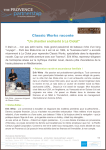
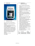
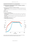
CAABA/MECCA-3.0
User Manual
Chemistry As A Boxmodel Application /
Module Efficiently Calculating the
Chemistry of the Atmosphere
Rolf Sander et al.
Air Chemistry Department
Max-Planck Institute of Chemistry
PO Box 3060, 55020 Mainz, Germany
[email protected]
http://www.mecca.messy-interface.org
This manual is part of the electronic supplement of our article
“The atmospheric chemistry box model CAABA/MECCA-3.0”
in Geosci. Model Dev. (2011), available at:
http://www.geosci-model-dev.net
Date: 2011-04-14
2
Sander et al.: CAABA/MECCA User Manual
Contents
7.2
The species files gas.spc and
aqueous.spc . . . . . . . . . . . . . . .
18
The equation files gas.eqn and
aqueous.eqn . . . . . . . . . . . . . . .
18
1 Introduction
3
2 Installation
3
7.3.1
Reaction numbers . . . . . . . .
19
. . . . . . . . . .
3
7.3.2
Markers and labels . . . . . . . .
19
2.1.1
Linux/Unix . . . . . . . . . . . .
3
7.3.3
2.1.2
MAC OS X . . . . . . . . . . . .
3
Creating a table of the chemical
mechanism . . . . . . . . . . . .
19
2.1.3
Windows . . . . . . . . . . . . .
3
Fortran95 files . . . . . . . . . . . . . . .
19
2.2
Prerequisites . . . . . . . . . . . . . . .
3
7.4.1
caaba.f90 . . . . . . . . . . . .
20
2.3
Installation . . . . . . . . . . . . . . . .
4
7.4.2
caaba mem.f90 . . . . . . . . . .
20
2.4
Troubleshooting . . . . . . . . . . . . . .
4
7.4.3
messy main control cb.f90 . .
20
7.4.4
messy jval box.f90 . . . . . . .
20
7.4.5
and
messy jval.f90
messy jval jvpp.inc . . . . . .
20
7.4.6
messy mecca box.f90 . . . . . .
20
7.4.7
messy sappho box.f90 . . . . .
21
2.1
System Requirements
3 Compiling
and
running
CAABA/MECCA box model
the shell script xcaaba
7.3
7.4
the
with
5
4 Selecting a chemical mechanism with the
shell script xmecca
6
7.4.8
messy sappho.f90 . . . . . . . .
21
4.1
Selecting a set of chemical reactions . .
10
7.4.9
messy semidep box.f90 . . . . .
21
4.2
Selecting a numerical integrator . . . . .
11
7.4.10 messy cmn gasaq.f90 . . . . . .
21
7.4.11 messy mecca aero.f90 . . . . .
21
How to expand the chemical mechanism
21
7.5.1
Adding a new gas-phase species .
21
7.5.2
Adding a new aqueous-phase
species . . . . . . . . . . . . . . .
21
7.5.3
Adding a new gas-phase reaction
21
7.5.4
Adding a new gas-phase photolysis reaction . . . . . . . . . . . .
22
Adding a new aqueous-phase reaction . . . . . . . . . . . . . . .
22
Adding a new Henry’s law equilibrium . . . . . . . . . . . . . .
22
Adding a new acid-base equilibrium . . . . . . . . . . . . . . . .
22
5 Plotting the model results with the ferret
software
11
7.5
6 Run CAABA/MECCA in special modes 11
6.1
6.2
Multiple model simulations and steadystate . . . . . . . . . . . . . . . . . . . .
11
Monte-Carlo . . . . . . . . . . . . . . . .
12
6.2.1
Performing Monte-Carlo simulations . . . . . . . . . . . . . . . .
12
Analyzing Monte-Carlo simulations . . . . . . . . . . . . . . . .
12
6.2.3
Variation of rate coefficients . . .
12
6.2.4
Changing the uncertainty factors
13
Lagrangian trajectories . . . . . . . . . .
13
6.3.1
Namelist parameters . . . . . . .
13
7.5.8
Adding a new label . . . . . . . .
22
6.3.2
Trajectory input file . . . . . . .
14
7.5.9
Adding a new emission . . . . . .
22
6.3.3
Photolysis rate file . . . . . . . .
15
7.5.10 Adding a new deposition
. . . .
23
6.3.4
Trajectory mode output . . . . .
15
7.5.11 Enlarging KPP . . . . . . . . . .
23
7.6
How to modify and add new scenarios .
23
7.7
How to modify the aerosol modes . . . .
23
7.8
Input files . . . . . . . . . . . . . . . . .
23
7.8.1
Tracer initialization file . . . . .
23
7.8.2
Photolysis initialization file . . .
24
How to add a new MESSy submodel . .
24
7.10 General programming guidelines . . . .
24
6.2.2
6.3
6.4
Tagging diagnostics and isotope modeling 15
7 Modifying CAABA/MECCA
7.1
Namelist files . . . . . . . . . . . . . . .
7.1.1
7.1.2
7.1.3
15
7.5.5
7.5.6
7.5.7
15
The CAABA namelist file
caaba.nml . . . . . . . . . . . .
15
The MECCA namelist file
mecca.nml . . . . . . . . . . . .
18
The JVAL namelist file jval.nml
18
7.9
Sander et al.: CAABA/MECCA User Manual
TRAJECT
(Lagrangian)
READJ
photolysis
3
CAABA Boxmodel
Global (3D) Model
MESSy Interface
MESSy Interface
JVAL
photolysis
SAPPHO
photolysis
SEMIDEP
emis, depos.
(insert here)
(insert here)
... other
submodels
MECCA
chemistry
Figure 1: Diagram showing MECCA as part of the CAABA box model or of a global model.
1
Introduction
MECCA (Module Efficiently Calculating the
Chemistry of the Atmosphere) is an atmospheric
chemistry module that contains a comprehensive
chemical mechanism with tropospheric and stratospheric chemistry of both the gas and the aqueous
phase (Sander et al., 2005). For the numerical integration, MECCA uses the KPP software (Sandu and
Sander, 2006).
To apply the MECCA chemistry to atmospheric conditions, MECCA must be connected to a base model.
As shown in Fig. 1, the base model can be a complex, 3-dimensional model (e.g. Jöckel et al., 2006)
but it can also be a simple box model. The connection is established via the MESSy interface (http://
www.messy-interface.org) developed by Jöckel et al.
(2005).
This manual describes how to install and work
with MECCA when it is connected to the box
model CAABA (Chemistry As A Boxmodel
Application).
This combination will be referred
to as “CAABA/MECCA”. The main features of the
CAABA box model are shown in Fig. 2. In addition
to MECCA chemistry, CAABA also contains several
other submodels, e.g. JVAL for calculating J-values,
SAPPHO for simplified and parameterized photolysis
rates, and SEMIDEP for simplified emission and
deposition.
2
Installation
This section can be skipped if CAABA/MECCA is already installed on your computer.
2.1
2.1.1
System Requirements
Linux/Unix
CAABA/MECCA has been tested successfully on several UNIX-like operating systems. The easiest installation is probably on a Linux PC since several auxiliary
programs are already included in a typical Linux distribution.
2.1.2
MAC OS X
CAABA/MECCA does not work with the version of
the sed program that is shipped with MAC OS X. Instead, it is necessary to install the GNU version of sed,
called gsed. This can be done using the MacPorts
(http://www.macports.org/). To ensure that gsed
is always executed when sed is called, a symbolic link
from sed to gsed can be created, e.g.:
sudo ln -s /opt/local/bin/gsed
/opt/local/bin/sed
Also, there may be problems executing the command
“echo -n” under OS X. If this is the case, the script
xmecca needs to be adjusted.
2.1.3
Windows
A native installation under Windows is neither recommended nor supported. However, it is possible
to execute the model in a virtual machine running
Linux on a Windows PC. The VMware Player, which
is needed to run the virtual machine, can be obtained from http://www.VMware.com. Information
how to obtain the Ubuntu Linux image file with the
CAABA/MECCA model (about 8 GB) from our ftp
site is given on the MECCA web page at http://www.
mecca.messy-interface.org.
2.2
Prerequisites
A Fortran95 compiler (mandatory): Several
compilers have been tested successfully: g95 (for
Linux), Lahey/Fujitsu (for Linux), Intel (for
Linux), Compaq (Alpha UNIX). Other compilers
can be used as well, if they accept standard
Fortran95 code. It should be noted that the g95
compiler for Linux is free and can be downloaded
from http://www.g95.org/.
4
Sander et al.: CAABA/MECCA User Manual
The Kinetic PreProcessor KPP (mandatory):
This flexible numerical integration package by
Sandu and Sander (2006) transforms the chemistry mechanism into a set of ordinary differential
equations (ODEs) in Fortran95 syntax. MECCA
needs the KPP version that is provided in the
mecca/kpp/ directory. Follow the instructions in
mecca/kpp/readme to install KPP.
Perl, tcsh, gawk, sed, and gmake (mandatory):
These UNIX tools are standard on Linux systems. Check that recent versions of them are
installed. Especially gawk may lead to strange
error messages. To test gawk, type:
gawk ’BEGIN {print match("X","[^a-z]")}’
The result should be “1”. However, you may get
“0” as the result on your system. Supposedly,
this is not a bug in gawk but a feature. You can
solve the problem by setting the environment
variable LC_ALL to “C”:
export LC_ALL=C
(if you use bash)
setenv LC_ALL C
(if you use tcsh)
When you try the gawk test again, it should
work fine.
LaTEX (optional): If you have LaTEX installed on
your computer, you can print a table (including
rate coefficients and references) of the currently
selected mechanism (see Sect. 7.3.3 for details).
netCDF library (strongly recommended): The
netCDF library is needed to create model output
in netCDF format. It can be obtained from http:
//www.unidata.ucar.edu/software/netcdf/.
Note that the *.mod files in the netCDF library
are compiler-specific. Thus, it is necessary to
create a netCDF library for each Fortran95
compiler and maybe also for each Fortran95
compiler version.
Software for manipulating or displaying netCDF
data is listed at: http://www.unidata.ucar.
edu/software/netcdf/software.html. If you
don’t have the netCDF library, you can still run
the model but produce only ASCII output.
netCDF tools (optional): Several tools are used to
analyse the netCDF output when the model is
run in the multirun (Sect. 6.1) or Monte-Carlo
(Sect. 6.2) mode. Specifically, the NCO programs
ncpdq, ncrcat, and ncks from http://nco.
sourceforge.net, the program ncdump, and
the program ncclamp from http://ncclamp.
sourceforge.net are needed.
ferret (optional): The ferret plotting program is
needed to plot the contents of the netCDF output using the ferret scripts in the jnl/ directory (see Sect. 5 for details). To ensure that
ferret finds all necessary files, you have to add
“./tools” to the FER_GO environment variable.
The ferret_paths*template files show how to
do this. For example, when using the tcsh, type:
setenv FER_GO "$FER_GO ./tools"
graphviz (optional): The graphviz program can be
used to create graphical visualizations of the reaction mechanism like Fig. 6.
fpc Pascal compiler (optional): To use the tagging diagnostics and isotope modeling features
(see Sect. 6.4 for details), version 2.2.0 or higher
of the free pascal compiler fpc from http://www.
freepascal.org/ is needed.
2.3
Installation
Once all prerequisites are fulfilled, you can install
CAABA/MECCA by simply unpacking the zip
archive:
unzip caaba 3.0.zip
Next, you have to check that all settings in Makefile
are correct. If necessary, edit the file: Choose a Fortran95 compiler (COMPILER), enter its name (F90) and
the compiler options (F90FLAGS). If you add a new compiler, check if you need to activate the C-preprocessor
option. To activate netCDF output, you also have to
edit the Makefile:
ˆ Check that the variable OUTPUT is set to NETCDF
(not to ASCII).
ˆ Enter the correct netCDF library information in
NETCDF_INCLUDE and NETCDF_LIB.
2.4
Troubleshooting
Should there be any problems
CAABA/MECCA installation, please
following:
with
check
the
the
ˆ Confirm that all prerequisites (see above) are fulfilled!
ˆ Confirm that the perl path in the first line of
sfmakedepend is correct. It should be the same
as the output of the command:
which perl
ˆ Confirm that the tcsh paths in the first lines of
xcaaba and xmecca are correct.
ˆ Confirm that the model code was unzipped successfully from the zip archive. Check for potential
problems during the unzipping process:
– Make sure that the directory structure has
not changed. Unfortunately, some unzipping programs seem to put all files into
one directory, ignoring the original directory
structure.
Sander et al.: CAABA/MECCA User Manual
5
ozone flux from free troposphere (SEMIDEP)
hν photolysis
(JVAL, SAPPHO
or READJ)
MECCA gasphase chemistry
sea-salt
particles
(MECCA aqueousphase chemistry)
MECCA gas/aqueous
mass transfer
sulfate
particles
(MECCA aqueousphase chemistry)
r.h.= 76 %
p = 1013 hPa
T = 293 K
production and
sedimentation of
sea-salt aerosol
emission and
deposition
(SEMIDEP)
marine
boundary
layer (mbl)
ocean
Figure 2: The CAABA box model
– Make sure that links have not been converted to files. For example, the output
of the command “file caaba.nml” should
tell you that caaba.nml is a symbolic link
to nml/simple/caaba.nml.
3
Compiling and running the
CAABA/MECCA box model
with the shell script xcaaba
First, go to the base directory of the model code (note
that all path names given in this manual are relative
to this base directory):
If you answer “y”, you can create a new chemical mechanism with xmecca as described in detail in Sect. 4.
However, for the first tests with CAABA/MECCA it
is recommended to answer “n” and use the simple default mechanism.
Choose an option:
s = Start from scratch
c = Compile
r = Run existing executable
h = Help
q = Quit
Choose “c” to compile the Fortran95 code. After a
successful compilation, xcaaba asks you to choose a
namelist file:
cd caaba 3.0
Next, the tcsh script xcaaba will guide you through
the process of running the box model, as illustrated in
Fig. 4. To execute xcaaba, type:
Choose a namelist file from
the nml/ directory:
...
./xcaaba
Namelists control the behaviour of CAABA/MECCA
during run-time, and editing them allows to define the
model setup at run-time (see Sect. 7.1). The default
is to use the same namelist as last time. For the first
tests, the file caaba_simple.nml can be chosen. The
active contents of the chosen namelist will be shown.
Next, xcaaba asks if you want to run the model:
xcaaba will ask several questions, and recommended
answers are given below. If you only press the Return
key, you select the default.
Start xmecca?
6
Sander et al.: CAABA/MECCA User Manual
Figure 3: Module structure of KPP-produced Fortran95 files. The arrows start at the module which is exporting
the PUBLIC variables and subroutines (which are shown in blue). They point to the module importing them via
the Fortran95 USE instruction. A dotted line represents an optional connection.
Run
y =
n =
q =
CAABA boxmodel with MECCA chemistry?
Yes (default)
No
Quit
Answer “y”, and the CAABA/MECCA model simulation will start. The flow control is illustrated in Fig. 5.
The model day and the current solar zenith angle (sza)
are printed on the screen during the model simulation.
The default is to integrate 8 days.
Save the output and model code
in output/ directory?
Answer “y”, and xcaaba will put the files
into a subdirectory with a name based on the
date and time of the model simulation, e.g.
output/2011-04-14-12:43:35/. It is recommended
to rename the subdirectory to a more descriptive
name.
4
Selecting a chemical mechanism with the shell script
xmecca
MECCA contains a very comprehensive set of chemical
reactions in both the gas phase and the aqueous phase.
For many applications, using the complete mechanism
will consume too much CPU time. Therefore, the shell
script xmecca has been written which allows to create a custom-made subset of the chemical mechanism
interactively. Normally, xmecca is called via xcaaba.
Sander et al.: CAABA/MECCA User Manual
7
xcaaba
full chemistry mechanism
(gas.spc, aqueous.spc,
gas.eqn, aqueous.eqn)
batch files
(*.bat)
selected chemistry mechanism
(mecca.spc, mecca.eqn)
kpp control file
(messy_mecca_kpp.kpp)
kpp-generated
Fortran files
(messy_mecca_kpp*.f90)
static, user-generated
Fortran files
(*.f90, *.inc)
xmecca
kpp
Fortran
compiler
(g95, lf95, ...)
executable
(caaba.exe)
Fortran namelists
(*.nml)
input data files
(*.nc)
execute
the model
model output
(*.nc, caaba.log)
Figure 4: Illustration of the tasks performed by xcaaba. xcaaba and all scripts called by xcaaba are shown on
a blue background. User-generated (static) input files are shown on a yellow background whereas automatically
generated temporary files are shown on a white background.
8
Sander et al.: CAABA/MECCA User Manual
Start
of model run
USE_TRAJECT
caaba_init
USE_MECCA
messy_init
USE_READJ
USE_SAPPHO
Start of time loop
t = t0
USE_JVAL
caaba_physc:
(calculations of
p, T, rh, sza, ...)
USE_TRAJECT
USE_SEMIDEP
messy_physc
No
USE_JVAL
USE_SAPPHO
t = tend ?
USE_MECCA
traject_init
mecca_init
...
readj_init
sappho_init
...
jval_init
...
traject_physc
semidep_physc
...
jval_physc
...
sappho_physc
mecca_physc
...
jval_finish
...
mecca_finish
...
sappho_finish
...
Yes
end of time loop
USE_JVAL
messy_finish
USE_MECCA
USE_SAPPHO
caaba_finish
USE_TRAJECT
traject_finish
End
of model run
BML
caaba.f90
BMIL
messy_main_control_cb.f90
SMIL
messy_*_box.f90
Figure 5: Flow control of a CAABA box model simulation
SMCL
messy_*.f90
Sander et al.: CAABA/MECCA User Manual
9
Cl2 (G7601)
ClNO3 (HET540)
hv (J7300)
BrNO2
HOCl (HET542)
hv (J7601)
DMS (G9700)
CF2ClBr
Cl (G7604)
hv (J7600)
hv (J7500)
OH (G7202)
CF3Br
OH (G7408)
CH2Br2
DMS (G9701)
hv (J7301)
HCHO (G7400)
HOBr (HET510)
Hg (G10703)
hv (J7401)
HO2 (G7200)
OH (G7607)
C2H2 (G7406)
I (G8700)
C2H4 (G7404)
IO (G8701)
HBr
CH2ClBr
hv (J7602)
NO (G7301)
CH3CHO (G7405)
OH (G7403)
CH3Br
hv (J7400)
Br
O3P (G7101)
CH3OOH (G7401)
OH (G7407)
CHBr3
hv (J7100)
hv (J7402)
OH (G7605)
O3 (G7100)
CHCl2Br
hv (J7603)
HgCl (G10705)
ClHgOBr
OH (G7606)
BrO (G7102a)
CHClBr2
NO2 (G7302)
hv (J7604)
CH3O2 (G7402b)
IBr
hv (J7200)
hv (J8700)
BrO (G7102b)
ClO (G7603a)
ClO (G7603b)
OH (G7204)
BrO
(G7303)
hv (J7301)
BrNO3
HCl (HET541)
BrCl
HO2 (G7201)
hv (J7000)
Br
chemistry
CH3O2 (G7402a)
HgBr (G10704)
O3P (G7203)
OH (G7204)
ClO (G7603c)
HOBr
H2O (HET520)
HCl (HET543)
HBr (HET510)
BrCl (G7600)
BrNO3 (G7300)
Br2
BrHgOBr
Br (G7300)
Cl (G7602)
Cl (G7602)
Hg (G10700)
Br (G7600)
Hg (G10702)
BrO (G10704)
HgBr
Cl (G10706)
Br (G10701)
HgBr2
ClHgBr
HgCl (G10707)
HgBr (G10701)
Figure 6: Visualization of the MECCA gas-phase bromine chemistry generated with the graphviz software.
However, you can also start it manually:
Modify gas.eqn with a replacement file?
cd mecca
./xmecca
Answer “0” unless you have written your own replacement file. More information about the replacement feature can be found in the file rpl/gas.rpl-example.
xmecca will ask several questions, and recommended
answers are given below. If you only press the Return
key, you select the default.
Choose a selection number or type a boolean
expression:
Select a batch file which defines
the chemistry mechanism that you
want to generate.
It is strongly recommended that you select a batch
file here. Batch files contain all the information that
xmecca needs to create a chemical mechanism. Several
batch files are available already, and it is also possible
to add your own batch files as explained at the end of
this section. If you do not select a valid batch file, you
can continue and answer all questions interactively as
described here.
How many aerosol phases?
For a gas-phase only mechanism, type “0”. For a mechanism with aqueous-phase chemistry in seasalt and in
sulfate particles, type “2”. Other values are possible if
they have been defined in subroutine define_aerosol
in messy_mecca_box.f90.
Now you can choose a subset of chemical reactions. A
few predefined standard selections are available. For
all other purposes, a batch file should be created, as
explained at the end of this section. Some of the predefined selections are:
EVAL: A mechanism that was used for the evaluation of the MECCA chemistry in the global model
ECHAM5/MESSy (Jöckel et al., 2006).
Minimum tropospheric chemistry: A very small
tropospheric mechanism.
Minimum MBL chemistry: A small mechanism
that contains aqueous-phase chemistry and
should only be used if the number of aerosol
phases is > 0.
For details about the selection, see Sect. 4.1.
Add Monte-Carlo factor to all rate
coefficients? [y/n/q, default=n]
10
Answer “n” here unless you want to perform MonteCarlo calculations, as described in Sect. 6.2.
Add diagnostic tracers to gas.eqn?
[q/0/?, default=0]
Answer “0”. Diagnostic tracers are usually only used
for 3-dimensional model runs.
Calculate accumulated reaction rates
of all equations? [y/n/q, default=n]
Answer “y” if you want to have all accumulated reaction rates in the model output. Otherwise, answer
“n”.
Tagging, doubling, both, or
none? [t/d/b/n/q, default=n]
Please use the default “n” here. The recommended
way to test tagging diagnostics and isotope modeling
is described in Sect. 6.4.
Run KPP?
Sander et al.: CAABA/MECCA User Manual
It is okay to delete these temporary files unless you
need them for debugging purposes.
When xmecca finishes successfully, the Fortran95 code
of your selected mechanism has been created. The
KPP-produced Fortran95 files (Tab. 2) are moved into
the mecca/smcl/ directory (with lower-case names).
An exception is messy_mecca_kpp_Model.f90, which
is produced by KPP but not needed for MECCA. The
modular structure of the KPP-produced Fortran95 files
is shown in Fig. 3.
If you need to create a chemical mechanism very often, it is quite tedious to answer all questions every time. To make this easier, you can copy the
template batch/example.bat to a new name (e.g.
batch/myfile.bat) and then enter your answers into
that batch file. Now you can create a new chemical
mechanism in batch mode with
./xmecca myfile
It is also possible to add the name of the batch file to
the xcaaba command:
Answer “y”.
./xcaaba myfile
Choose an integrator [q=quit,
default=rosenbrock_posdef]:
4.1
The default integrator is strongly recommended (see
Sect. 4.2 for details). Next, KPP will create several
Fortran95 files.
Remove indirect indexing with decomp?
[y/n/q, default=n]
If this question shows up, answer “n”.
Create LaTeX listing of selected mechanism?
[y/n/q, default=n]
If you answer “y” here, a table of the current reaction mechanism will be produced. Only the selected
reactions will be listed. The table also contains the
rate coefficients and their references, as described in
Sect. 7.3.3.
Create graphviz plots of selected
mechanism? [y/n/q, default=n]
If you have the “dot” program from the graphviz
software installed, you can create graphical visualizations of the reaction mechanism. As an example, the graphviz-generated plot of gas-phase bromine
chemistry is shown in Fig. 6. For more information, look at the files xgraphvizall, xgraphviz, and
spc_extract.awk in the mecca/graphviz/ directory.
Do you want to delete the temporary
xmecca files?
Selecting a set of chemical reactions
All chemical reactions are marked. Each marker
consists of several labels, which contain information about the domain (troposphere/stratosphere), the
phase where the reaction occurs (gas/aqueous), its relevant chemical elements, and more. See Sect. 7.3.2 for
a complete list of labels. To define a set of chemical
reactions, you can either choose a pre-defined selection
by number or enter a boolean expression based on the
labels. Boolean expressions are typed in gawk syntax.
The most important operators and expressions are:
&& = AND
|| = OR
! = NOT
() = parentheses
1 = TRUE
0 = FALSE
For example, to select all gas-phase reactions (G) except for those including halogens (Cl, Br, I), type:
G && !Cl && !Br && !I.
It is important to understand the logic behind this selection mechanism. The expression “Cl && Br” selects
only those reactions that contain chlorine and bromine.
Similarly, the expression “G && Het” selects only those
reactions that occur in the gas phase and are heterogeneous. However, since no reaction has both the “G”
and the “Het” label, this results in an empty mechanism. If you want a mechanism that contains both gasphase and heterogeneous reactions, you must select all
reactions that contain either the label “G” or the label
“Het”, i.e. you must use the expression “G || Het”.
Sander et al.: CAABA/MECCA User Manual
4.2
Selecting a numerical integrator
Several numerical integrators are defined in the
subdirectory mecca/kpp/int/ and can be used
with KPP. The default is the positive definite
Rosenbrock solver with automatic time-step control
(rosenbrock_posdef). It is very robust and capable
of integrating very stiff sets of equations (e.g. chemical mechanisms including both gas- and aqueous-phase
chemistry). Although a Rosenbrock solver with manual time-step control (ros2_manual) is also available,
it is strongly recommended not to use it for stiff sets of
equations. If you choose it, you do so at your own risk!
11
go rxnrates_scaled.jnl OH
To plot results from previous simulations which
are saved in the output/ directory, edit the file
setmodelrun.jnl and enter the paths of the directories in the “GO _define_sensi” command. To compare model simulations, you can enter two or more
“GO _define_sensi” commands in setmodelrun.jnl.
To plot the difference between model simulations, activate the line “DEFINE SYMBOL diffplot TRUE” in
setmodelrun.jnl.
6
5
Plotting the model results
with the ferret software
If you have chosen netCDF output, you can plot
the model results with the ferret program (http:
//ferret.wrc.noaa.gov/Ferret/). Change into the
jnl/ directory, then start the program by typing
“ferret”. When ferret has started, you can plot the
gas-phase species of the latest model simulation with
the ferret script xxxg.jnl by typing:
go xxxg.jnl
Similarly, xxxa.jnl can be used to plot aqueous-phase
species:
go xxxa.jnl
The file xxxa.jnl accepts several parameters to modify
the plots. The first parameter should be “0d” for plotting box model results. The second parameter can be
set to “mpl” or “mpm” in order to plot either aqueousphase concentrations in mole per liter or mixing ratios
in mole per mole, respectively. The third parameter
defines the aerosol bin. With two aerosol bins, “A01”
refers to sulfate particles, and “A02” to sea-salt particles. For example, type:
go xxxa.jnl 0d mpl A02
Photolysis rate coefficients can be plotted with
jval.jnl:
go jval.jnl
If the calculation of accumulated reaction rates had
been switched on in xmecca (see Sect. 4), plots of the
reaction rates can be made. One possibility is to plot
all reactions with:
go rxnrates.jnl
Alternatively, it is possible to plot only the production
and destruction rates for a certain species, e.g. for OH:
Run CAABA/MECCA in special modes
In the base configuration described so far,
CAABA/MECCA calculates the temporal evolution of the chemistry inside an air parcel. This is ideal
for sensitivity studies analyzing the effect of individual
reactions inside a large chemical mechanism. For other
applications, some special modes exist as described
below.
6.1
Multiple model simulations and
steady-state
The so-called “multirun” mode performs multiple
model simulations, each of them terminating when a
steady-state has been reached. This is useful to calculate the steady-state concentrations of short-lived
species when the concentrations of longer-lived species
(e.g. non-methane hydrocarbons) are known from measurements. The default termination condition is that
the relative change of OH and HO2 between two model
time steps is less than 10−6 s−1 . If necessary, this can
be changed in the function steady_state_reached in
messy_mecca.f90. To avoid that the concentrations of
long-lived species change from their initial values, they
can be fixed in the file mecca/messy_mecca_kpp.kpp
by adding them to the “#SETFIX” line. A tracer
initialization file (see Sect. 7.8.1) and a photolysis
initialization file (see Sect. 7.8.2) must be available
in the multirun/input/ directory. As an example, the files example_*.nc are available. To create such input netCDF files from ASCII files, the
script asc2ferret4nc.tcsh can be used. Finally,
since the multirun mode needs “ncks” from the
netCDF Operators (NCO) software, it must be ensured that this program is available. After these preparations, the multirun mode can be entered by running xcaaba and answering “Choose a namelist file”
with “m”. The user can either select one input file
or make model simulations for all input files in the
multirun/input/ directory. For each input netCDF
file, the script multirun.tcsh is called. For each
time step contained in the input file, multirun.tcsh
first creates a suitable namelist file caaba.nml and
12
Sander et al.: CAABA/MECCA User Manual
then performs a CAABA/MECCA model simulation. The namelist file contains values for temperature and pressure taken from the input netCDF file.
In addition, the steady-state option is switched on
with “l_steady_state_stop = T”, and the submodel
READJ is activated and used with “USE_READJ = T”
and “photrat_channel = ’readj’”. After all model
simulations have finished, a summary of the output is placed in the output directory. The name
of the output directory will be based on the
name of the input netCDF file, e.g. when the file
example_small.nc is used, the output will be in
output/multirun/example_small/.
6.2
6.2.1
Monte-Carlo
The most efficient way to analyze a large number of
Monte-Carlo simulations is to use the steady-state option and only compare the final values of the different model simulations, not the individual time series.
The ferret script montecarlo.jnl can be used to create scatter plots of concentrations vs rate coefficients.
It also plots linear regression lines for all comparisons
above a given threshold of the coefficient of determination (r2 ). Note, however, that r2 is only an indicator of
the goodness of a linear correlation. It is also possible
that the dependence of a species on a rate coefficient
is nonlinear. For an exhaustive analysis of the model
results, the threshold in the file scatterplot_mc.jnl
can be set to zero, thus creating scatter plots of all
species against all rate coefficients.
Performing Monte-Carlo simulations
In the Monte-Carlo mode, several CAABA/MECCA
simulations are performed, with each individual simulation using slightly different rate coefficients. To
activate it, you first have to create a new chemistry
mechanism with xmecca (see Sect. 4) and answer the
question “Add Monte-Carlo factor to all rate coefficients” with “y” (e.g. using the batch file mcfct.bat).
This will start the gawk script mcfct.awk, which adds
Monte-Carlo factors to the rate coefficients in the equation file. Next, the xcaaba script can be used to start
the simulations. A suitable namelist for this purpose
is caaba_mcfct.nml. The script montecarlo.tcsh
in the directory montecarlo/ will now perform the
Monte-Carlo model simulations. The default is to
make 100 model simulations. To choose another value
(up to 9999), change the definition of maxline in
montecarlo.tcsh.
6.2.2
Steady-state calculations
Analyzing Monte-Carlo simulations
After performing the model simulations, the resulting netCDF files are merged (using the tools ncpdq,
ncclamp, and ncrcat) and then stored in the output directory with a name based on the date and
time of the model simulations, e.g. $outputdir =
output/montecarlo/2010-06-24-16:29:00. The final concentrations and rate coefficients of all simulations are summarized in caaba_mecca_c_end.nc
and caaba_mecca_k_end.nc. Results of the individual simulations can be found in the directories
$outputdir/runs/*.
Time series
If the model is set up to run for a fixed length (e.g.
using the default of runtime_str = 8 days), the
time series of all simulations can be plotted together
with ferret by activating the lines for Monte-Carlo in
setmodelrun.jnl. However, these plots become illegible if more than about 5 simulations are made.
6.2.3
Variation of rate coefficients
In each individual Monte-Carlo simulation j, all rate
coefficients ki are varied by a Monte-Carlo factor:
x
MC
ki,j
= ki × fi i,j
(1)
MC
Here, ki,j
is the rate coefficient of reaction i used in
the Monte-Carlo simulation j. It is defined as the product of the recommended value ki and the Monte-Carlo
x
factor fi i,j . This Monte-Carlo factor consists of two
parts, the uncertainty factor fi and the exponent xi,j :
The uncertainty factor fi
The uncertainty factor fi describes the uncertainty of
the measured (or estimated) rate coefficient ki . Its
value can usually be found in publications of laboratory
studies or summaries like the JPL evaluation (Sander
et al., 2006).
The tables of the IUPAC evaluations (e.g. Atkinson
et al., 2006) list the decadic logarithm lg(fi ) of the
uncertainty factor, which they call “∆ log k”.
Sometimes an absolute uncertainty is quoted instead of
an uncertainty factor, e.g. k = 2 ± 0.2 or k = 2 ± 10%.
In this case we define fi such that the upper limit is
reached when multiplied with ki , i.e. in the current
example fi = (2 + 0.2)/2 = 1.1.
The uncertainty factor is defined in the equation files
(*.eqn) in a comment starting with the paragraph symbol. Three different syntax types are possible:
ˆ If there is just one § sign, (e.g. “{§1.1}”), the
value inside the curly braces is the uncertainty
factor fi .
ˆ With two § signs, (e.g. “{§§0.04}”), the value
inside the curly braces equals lg(fi ).
ˆ If there is only a § sign (“{§}”) but no number,
the uncertainty factor is set to the default value
of fi = 1.25.
Sander et al.: CAABA/MECCA User Manual
13
the output in caaba.log.
After these tests,
montecarlo_check must be switched off again to
allow normal model simulations.
6.3
Lagrangian trajectories
CAABA can be used as a Lagrangian trajectory box
model (Riede et al., 2009). The usual combination of
submodels for this purpose includes the CAABA submodel TRAJECT for the processing of trajectory information, MECCA for atmospheric chemistry, and JVAL
for photolysis rate calculation. All important settings
for trajectory calculations can be made via the namelist
file plus a few external files.
Figure 7: Example histogram of normally-distributed
random numbers.
The Monte-Carlo exponent xi,j
There is one Monte-Carlo exponent xi,j (variable
“mcexp” in the code) for each rate coefficient ki and
for each individual Monte-Carlo simulation j. The values of xi,j are normally-distributed random numbers
centered around zero (see Fig. 7), and produced with
the Marsaglia polar method (http://en.wikipedia.
org/wiki/Marsaglia_polar_method). As input for
the Marsaglia polar method, uniformly distributed random numbers between 0 and 1 calculated with either the standard Fortran95 function RANDOM NUMBER
or the Mersenne Twister algorithm (Matsumoto and
Nishimura, 1998) are used.
6.2.4
Changing the uncertainty factors
The uncertainty factors can be changed by modifying
the equation files, as shown in Sect. 7.3. Note that predefined rate coefficients (e.g. k_HO2_HO2) already contain an uncertainty factor and there must not be an
additional factor in the reaction where they are used.
In some cases, it may be useful to vary only one or a
few rate coefficients. To do this, it is first necessary to
find the correct indices of mcexp(...) in mecca.eqn
(note that these indices may change when creating
a new mechanism with xmecca). As an example, to
vary only the rate coefficients that use mcexp(40)
and mcexp(50), the following lines can be added to
subroutine mecca_init in messy_mecca_box.f90 after
CALL define_mcexp:
6.3.1
Namelist parameters
A
namelist
template
can
be
found
in
nml/caaba_traject_example.nml.
After copying
the namelist file to a new name in the same directory
and altering the settings, it will be available when
running CAABA via xcaaba. There are standard and
trajectory-exclusive namelist parameters to be set:
ˆ Submodel switches (mandatory):
The
trajectory mode of CAABA requires that
USE_TRAJECT = T,
USE_MECCA = T,
and
USE_JVAL = T and/or USE_SAPPHO = T. One of
the two photolysis rate models is sufficient, but
it is also possible to run them in parallel (see
also photrat_channel). If the use of external
photolysis rates is desired, USE_JVAL = T is
mandatory since the scaling of photolysis rate
coefficients is currently only implemented for
JVAL. For the application in Riede et al. (2009),
the submodel SEMIDEP was switched off.
ˆ Scenarios (optional): The use of scenarios is
optional in trajectory mode. When using external input for chemical initialization and photolysis rates, they can be used to supplement default
values for unspecified photolysis rate coefficients
or initial mixing ratios.
ˆ Photolysis rate channel: Since the scaling of photolysis rate coefficients is currently only implemented for JVAL, choose
photrat_channel = ’jval’ when planning to
prescribe photolysis rates.
DO i=1, MAX_MCEXP
IF ((i/=40).OR.(i/=50)) mcexp(i) = 0.
ENDDO
ˆ Trajectory input (mandatory):
The
path to the netCDF file containing trajectory waypoints should be specified as
input_physc = ’traject/example_traj.nc’.
For its structure, see section 6.3.2.
To verify that the rate coefficients are modified in
the Monte-Carlo simulations, it is possible to temporarily activate the subroutine montecarlo_check
in template_messy_mecca_kpp.f90 and check
ˆ Tracer initialization (optional): Tracer mixing ratios can be initialized with an external netCDF file by specifying the path to
it: init_spec = ’traject/example_init.nc’.
For its structure, please refer to section 7.8.1.
14
Sander et al.: CAABA/MECCA User Manual
model runtime along the trajectory. runlast defines the start of the CAABA simulation counted
backwards in time from the trajectory end, i.e.
runlast = 4.5 means “calculate the last 4.5
days of the trajectory”. The unit is days.
The parameter runtime_str defines the overall model simulation time. Thus, runlast and
runtime_str combined select any desired part of
the trajectory.
Without an external file for tracer initialization,
tracers mixing ratios are initialized by box model
default or by the chosen scenario.
ˆ Photolysis rates (optional):
To scale
photolysis rates to prescribed J(NO2 ) values, specify the path to the respective file as
input_jval = ’traject/example_jval.nc’.
For its structure, see 6.3.3.
ˆ Variable names (partly mandatory): There
are default trajectory variable names designated
in CAABA. They can be selectively changed by
providing alternative variable names. Here is a
list of trajectory variables, their default name,
and respective examples how to specify an alternative variable name:
quantity
default alternative
longitude
LON
vlon = ’LON_TR’
latitude
LAT
vlat = ’LAT_TR’
pressure
PRESS
vpress = ’P’
temperature
TEMP
vtemp = ’TM1’
rel. humidity
RELHUM vrelhum = ’rh’
spec. humidity
vspechum = ’sh’
For only one of the two humidity variables, an
alternate name may be active in the namelist.
This is the variable that is subsequently used as
humidity and that is internally converted to relative humidity if necessary. When specific humidity is provided, then both specific humidity and relative humidity are written to output
caaba_physc.nc, since CAABA uses relative humidity internally. When relative humidity is provided, only relative humidity will be written to
output.
ˆ Humidity definitions (optional): To switch
from the traditional relative humidity definition
to the WMO definition, l_relhum_wmo = T can
be selected (see also Sect. 6.3.4).
ˆ Use relative humidity? (optional): By default, the relative humidity is used to calculate
the concentration of water vapor c(H2 O). If
l_ignore_relhum = T, then the relative humidity is ignored, and c(H2 O) must be initialized in
SUBROUTINE x0 (either directly or via external
chemical initialization).
ˆ Water vapor saturation pressure (optional): By default, the parameterizations from
Murphy and Koop (2005) for both, vapor pressure over liquid and over ice are used. To
use the saturation vapor pressure parameterizations from EMAC, choose the namelist entry
l_psat_emac = T,
ˆ Integration
time
(optional):
timesteplen_str sets the integration and
output time step. See also Sect. 7.1.1.
ˆ Selecting trajectory parts (optional): Two
namelist parameters allow flexible selection of the
6.3.2
Trajectory input file
The trajectory information is provided to CAABA
via an external netCDF file specified in the namelist
by input_physc.
A sample file is available at
traject/example_traj.nc.
The file should contain a time origin in ’seconds/minutes/hours/days
since yyyy-mm-dd hh:mm:ss’, where the seconds
in the time string are optional, for example:
"MINUTES since 2000-01-19 08:00:00". The file
must contain at least two trajectory waypoints and the
following time-dependent variables:
quantity
longitude
latitude
pressure
temperature
(rel. humidity)
(spec. humidity)
default name
LON
LAT
PRESS
TEMP
unit
degrees east
degrees north
Pascal
Kelvin
1
kg/kg
Of the two humidity quantities, only one needs to be
present. If specific humidity is given, it is converted
to relative humidity (RH) within CAABA. Depending
on the namelist parameter l_relhum_wmo, either the
traditional definition of relative humidity
RH =
pH2 O (T )
,
psat (T )
(2)
or the WMO definition (Jacobson, 1999)
RH =
p − psat (T )
ωv
pH2 O (T )
×
=
ωvs
p − pH2 O (T )
psat (T )
(3)
is assumed, with p = atmospheric pressure, pH2 O =
water vapor partial pressure, psat = water vapor saturation pressure, ωv = water vapor mass mixing ratio,
and ωvs = saturation water vapor mass mixing ratio in
dry air. We calculate the latter two as:
ωv
=
ωvs
=
q
1−q
M (H2 O)
psat (T )
×
,
M (air)
p − psat (T )
(4)
(5)
using the temperature-dependent saturation water vapor pressure psat (T ), and the molar masses M of water
and dry air. There are two parameterization schemes
available for the water vapor saturation pressure, which
can be selected by namelist (see Sect. 6.3.1).
Sander et al.: CAABA/MECCA User Manual
6.3.3
Photolysis rate file
It is possible to scale photolysis rate coefficients via prescribed J(NO2 ) values from a netCDF file. An example
is available at traject/example_jval.nc. The name
in the netCDF file must be J_NO2. The files specified in
input_jval (e.g. example_jval.nc) and input_physc
(e.g. example_traj.nc) must both refer to exactly the
same trajectory because the J values are read into the
model at the same times as other trajectory information.
6.3.4
Trajectory mode output
Output along the trajectory is written to
caaba_messy.nc. There are some special variables
written out in addition to the default caaba_messy.nc
output. They are listed in the second part of Tab. 1.
Specific humidity (q) is only written to output if it was
provided as input.
6.4
Tagging diagnostics and isotope
modeling
Before using the tagging feature, please make sure
that version 2.2.0 or higher of fpc (Free Pascal compiler, http://www.freepascal.org/) is installed and
configured on your system. To create an isotopically
tagged chemical mechanism with xmecca, the batch
file iso_example.bat can be used. Note that tagdbl
is set to “d” (doubling) here. The alternative option “t” (tagging) is not intended to be used in boxmodel simulations and thus currently disabled. Before
running CAABA/MECCA, the execution of the doubling code has to be enabled by setting l_dbl=T in
the &CTRL namelist in mecca.nml. In this configuration, the model simulation will produce additional files
caaba_mecca_dbl_*.nc containing output from the
doubling, e.g., concentrations of isotopologues and isotope ratios. The batch file iso_example.bat contains
a simple example of the 12 C/13 C isotopes of methane
tagging. Further tagging configurations can be found
by running xmecca interactively (without using a batch
file) and answering “d” to the question about doubling/tagging. To obtain further details, please contact
Sergey Gromov <[email protected]>.
7
Modifying CAABA/MECCA
The CAABA/MECCA model simulation can be modified by changing the input files (*.nc), the namelist
files (*.nml), the species files (*.spc), the equation files
(*.eqn) and the Fortran95 files (*.f90). Frequently
applied changes are:
ˆ Change the model time (start, stop), location
(lon, lat), and/or meteorology (p, T , RH) →
Sect. 7.1.1
15
ˆ Add, delete, and change individual chemical reactions → Sect. 7.5
ˆ Create or change the set of photolysis rate coefficients → Sect. 7.6
ˆ Create or change the set of emission fluxes →
Sect. 7.6
ˆ Create or change the set of deposition velocities
→ Sect. 7.6
ˆ Create or change the set of initial mixing ratios
→ Sect. 7.6
ˆ Change the model initialization using input files
→ Sect. 7.8
The following sections describe typical (mostly minor) changes to the model that are probably needed
by many users. If you would like to make extensive
changes/additions to the model, please follow also the
general programming guidelines described in Sect. 7.10.
7.1
Namelist files
Fortran95 namelist files allow modifications of the
model simulation without having to recompile the
source code.
7.1.1
The CAABA namelist file caaba.nml
The file caaba.nml contains the namelist &CAABA. Here
individual parts of the CAABA model (the so-called
“MESSy submodels”) can be switched on or off. It is
important that the following switches are set to “T”
(=true):
USE_MECCA
= T
USE_SAPPHO = T
USE_SEMIDEP = T
To use the photolysis rate coefficients from SAPPHO
in MECCA, set:
photrat_channel = ’sappho’
Alternatively, you can switch on the JVAL
submodel with USE_JVAL = T and then select
photrat_channel = ’jval’. It is fine to switch on
both the JVAL and the SAPPHO submodel, which
can be useful for a comparison. However, only the
values selected by photrat_channel are used for the
MECCA chemistry.
You can define the model start, runtime, and time step,
e.g.:
model_start_day = 90.
runtime_str
= ’10 days’
timesteplen_str = ’15 minutes’
16
Sander et al.: CAABA/MECCA User Manual
variable
lon
lat
lev
time
lon_tr
lat_tr
press
temp
relhum
spechum
sza
J_NO2_x
localtime
year_loc
month_loc
day_loc
hour_loc
min_loc
sec_loc
Table 1: List of trajectory mode
unit
(dummy 3-D x-coordinate)
(dummy 3-D y-coordinate)
(dummy 3-D z-coordinate)
<time unit> since <time origin>
degrees east
degrees north
Pa
K
1
kg/kg
deg
1/s
(same as time)
If you don’t set these, the default is a model start on
day-of-year (“Julian Day”) 80, a model simulation duration of 8 days, and an output time step of 20 minutes. The timesteplen_str value can be given as any
integer or floating point and in the units of seconds,
minutes, or hours.
As an alternative, it is possible to stop the model simulation when a steady state has been reached. This is
normally used in the “multirun” mode (Sect. 6.1):
l_steady_state_stop = T
The default location of the model simulation (latitude,
longitude) is 45◦ N and 0◦ E. It can be changed with
e.g.:
degree_lat = 82. ! Alert
degree_lon = 297. ! Canada
Changing the latitude only affects photolysis calculations (via the zenith angle calculations). The longitude
is only used for Lagrangian trajectory calculations.
The values of temperature (temp), pressure (press),
relative humidity (relhum), and the height of the
boundary layer (zmbl) can be defined, e.g.:
temp
press
relhum
zmbl
=
=
=
=
293.
101325.
0.81
1000.
!
!
!
!
[K]
[Pa]
[1]
[m]
The values shown here are the default values as defined
in caaba_mem.f90.
In the submodel SEMIDEP, emissions are distributed
evenly into the well-mixed boundary layer of height
output variables.
notes
UTC
longitude
latitude
pressure
temperature
relative humidity (RH)
specific humidity (q)
solar zenith angle
NO2 photolysis rate
local time at trajectory position
year of local time
month of local time
day of local time
hour of local time
minute of local time
second of local time
zmbl. Note that CAABA is a box model, and changing
zmbl has no other effects than this.
It is possible to initialize chemical species from a
netCDF file (see Sect. 7.8.1). To activate this feature,
define a valid input file name, e.g.:
init_spec = ’traject/example_init.nc’
If the submodel READJ is switched on, a netCDF file
containing J-values must be defined (see Sect. 7.8.2).
In addition, an index can be defined, if the netCDF file
contains data for more than one time step, e.g.:
init_j = ’multirun/input/example_small.nc’
init_j_index = 25
To facilitate running CAABA under different boundary conditions, so-called “scenarios” can be defined. Currently, there are scenarios for photolysis (photo_scenario), initialization (init_scenario),
emission (emission_scenario), and dry deposition
(drydep_scenario):
photo_scenario
init_scenario
emission_scenario
drydep_scenario
=
=
=
=
’MBL’
’MBL’
’MBL’
’MBL’
Possible values (“MBL” is used here as an example) for the scenarios can be found in the variable
list_of_scenarios in caaba.f90. Note that values have not yet been assigned for all scenarios. See
Sect. 7.6 for details about scenarios.
Finally, it is possible to skip the chemistry calculations
with KPP completely. This is only useful for debugging:
l_skipkpp = T
Sander et al.: CAABA/MECCA User Manual
Table 2: List of CAABA/MECCA Fortran95 files
CAABA box model related files
caaba.f90
main box model file
caaba_io.f90
input/output
caaba_io_netcdf.inc
netCDF input/output
caaba_io_ascii.inc
ASCII input/output
caaba_mem.f90
declaration of CAABA variables
messy_main_control_cb.f90
flow control
messy_jval_box.f90
connection of JVAL to CAABA
messy_mecca_box.f90
connection of MECCA to CAABA
messy_mecca_dbl_box.f90
for isotope modeling
messy_mecca_tag_box.f90
for isotope modeling
messy_readj_box.f90
connection of READJ to CAABA
messy_sappho_box.f90
connection of SAPPHO to CAABA
messy_semidep_box.f90
simplified emission and deposition, including connection of
SEMIDEP to CAABA
messy_traject_box.f90
trajectory calculations
static core files (generic)
messy_cmn_gasaq.f90
common definitions for gas/aqueous mass transfer
messy_cmn_photol_mem.f90
common definitions for photolysis
messy_main_blather.f90
print utilities
messy_main_constants_mem.f90
physical constants
messy_main_rnd.f90
random number generation
messy_main_rnd_lux.f90
(file exists but is not not used with CAABA)
messy_main_rnd_mtw.f90
Mersenne-Twister random numbers
messy_main_timer.f90
timer
messy_main_tools.f90
auxiliary functions
messy_main_tools_kp4_compress.f90 (file exists but is not not used with CAABA)
static core files (submodel-specific)
messy_jval.f90
calculation of J-values
messy_jval_jvpp.inc
include file for JVAL
messy_readj.f90
read J-values
messy_sappho.f90
simplified and parameterized photolysis rate coefficients
static MECCA core files
messy_mecca.f90
MECCA core
messy_mecca_aero.f90
aerosol chemistry
messy_mecca_khet.f90
(file exists but is not used with CAABA)
messy_mecca_dbl_parameters.inc
for isotope modeling
messy_mecca_tag_parameters.inc
for isotope modeling
KPP- and xmecca-produced files
messy_mecca_kpp.f90
a wrapper for the KPP files
messy_mecca_kpp_function.f90
ODE function
messy_mecca_kpp_global.f90
global data headers
messy_mecca_kpp_initialize.f90
initialization
messy_mecca_kpp_integrator.f90
numerical integration
messy_mecca_kpp_jacobian.f90
ODE Jacobian
messy_mecca_kpp_jacobiansp.f90
Jacobian sparsity
messy_mecca_kpp_linearalgebra.f90 sparse linear algebra
messy_mecca_kpp_monitor.f90
equation info
messy_mecca_kpp_parameters.f90
model parameters
messy_mecca_kpp_precision.f90
arithmetic precision
messy_mecca_kpp_rates.f90
user-defined rate laws
messy_mecca_kpp_util.f90
utility input-output
17
18
7.1.2
Sander et al.: CAABA/MECCA User Manual
The MECCA namelist file mecca.nml
The file mecca.nml contains the namelists &CTRL_KPP
and &CTRL (the namelist &CPL is not used in connection with CAABA). &CTRL_KPP is used for finetuning the numerical integration. The default selection
icntrl(3) = 2 should normally be suitable.
7.1.3
The JVAL namelist file jval.nml
The file jval.nml contains several namelists. When
JVAL is run as a submodel for CAABA, only the control namelist (&CTRL) is used. Normally, there is no
need to change the default settings.
7.2
The species
aqueous.spc
files
gas.spc
and
The files *.spc declare chemical species for KPP. All
species that may occur in an equation must be declared
here. Additional dummy species may also be declared
here.
Gas-phase species are declared in gas.spc. Examples
for gas-phase species are O2, O1D, and NO2. The names
of lumped species start with “L”. The names of species
with two or more carbon atoms are taken from the
master chemical mechanism (MCM).
MECCA also includes aqueous species which are declared in aqueous.spc. The names of cations end
with “p” for plus. The names of single-charge anions end with “m” for minus. Doubly-charged anions end with “mm”. Examples for aqueous species
are “H2O2” (H2 O2 ), “Hp” (H+ ), “NO3m” (NO−
3 ), and
“SO4mm” (SO2−
4 ).
All aqueous-phase species have the suffix “_a##”, which
is a placeholder for the aerosol phase. xmecca replaces
it by a two-digit number, e.g., “_a01” for the accumulation or “_a02” for the coarse mode. This allows
separate chemistry calculations for aerosol particles of
different size and composition.
All species are defined here with #DEFVAR, i.e. KPP
considers them as prognostic variables. To treat a
species as a constant (e.g. CO2 ), it can be added to the
#SETFIX command in the file messy_mecca_kpp.kpp.
The declarations in #DEFVAR can and should remain
unchanged when altering #SETFIX.
7.3
The equation files gas.eqn and
aqueous.eqn
The equation files *.eqn define the chemical reaction
mechanism for KPP. After making any changes to the
equation files, it is always necessary to execute KPP
via xmecca again. Each reaction occupies one line in
this file. An example is:
<G1000> O2 + O1D = O3P + O2 : {%StTrG}
3.3E-11*EXP(55./temp); {&1945}{§1.1}
Note that, although split here in this manual, this is
only 1 line in the equation file. The line starts with the
reaction number, which is enclosed in angle brackets
“<...>” (see Sect. 7.3.1). The second part (up to the
colon) defines the reaction, and the third part (between
the colon and the semicolon) defines the rate coefficient.
The lines may also contain comments. Comments in
equation files are either enclosed in curly braces, or the
comment line starts with “//”. When using xmecca,
some comments have a special meaning. Comments
starting with the percent symbol “{%...}” are markers (see Sect. 7.3.2). Comments starting with the ampersand “{&...}”, the “at”-symbol “{@...}”, or the
dollar “{$...}” are used to store information for the
listing of reactions, as explained in Sect. 7.3.3. Comments starting with the paragraph symbol “{§...}”
are defining uncertainties of the rate coefficients for
Monte-Carlo calculations (see Sect. 6.2).
If the definition of a rate coefficient is very complex, it
can be stored in a Fortran95 variable and the variable is
put into the gas.eqn file. For example, the rate of the
self reaction of HO2 is quite complex since it depends
on humidity. It is predefined and the reaction line can
be simplified to:
HO2 + HO2 = H2O2 : k_HO2_HO2;
The declaration and definition of k_HO2_HO2 are also
in the gas.eqn file. They can be found in the so-called
KPP “inline types” F90_GLOBAL and F90_RCONST, e.g.:
#INLINE F90_GLOBAL
REAL :: k_HO2_HO2
#ENDINLINE
#INLINE F90_RCONST
k_HO2_HO2 = (1.5E-12*EXP(19./temp)+ &
1.7E-33*EXP(1000./temp)*cair)* &
(1.+1.4E-21* &
EXP(2200./temp)*C(KPP_H2O))
#ENDINLINE
Another method to add reaction rates with complex dependencies are Fortran95 functions. This is
done for example for the oxidation of S(IV) by H2 O2
(k_SIV_H2O2). A function call is given as the rate expression in the *.eqn file. These functions are defined
with the “inline type” F90_RATES:
#INLINE F90_RATES
ELEMENTAL REAL(dp) FUNCTION k_SIV_H2O2 &
(k_298,tdep,cHp,temp)
...
END FUNCTION k_SIV_H2O2
#ENDINLINE
Sander et al.: CAABA/MECCA User Manual
7.3.1
Reaction numbers
Each reaction in an equation file has a unique reaction
“number” (number is not quite correct, since letters
are included as well), which is enclosed in angle brackets, e.g.: “<G1000>”. The reaction number starts with
one or more upper case letters denoting the type of
reaction. The following types exist:
A
H
EQ
G
J
HET
aqueous-phase reactions
Henry’s law (dissolution and evaporation)
equilibria in the aqueous phase (forward and
backward reactions of acid/base and other
equilibria)
gas-phase reactions
J-values of photolysis reactions
heterogeneous reactions (e.g. on polar
stratospheric clouds)
The type is followed by a sequence of 3 or 4 digits.
The first digit is the number of the main element of
the reaction. The following numbers are used:
1)
2)
3)
4)
5)
6)
7)
8)
9)
10)
O
H
N
C
F
Cl
Br
I
S
Hg
Oxygen
Hydrogen
Nitrogen
Carbon
Fluorine
Chlorine
Bromine
Iodine
Sulfur
Mercury
Out of those elements that occur in a reaction, the one
with the highest number is called the main element.
Accordingly, the second digit is determined by the element with the second highest number (or set to zero
if there is no second element in the reaction). There is
one exception in this numbering scheme: For the carbon group, the second digit is the number of C atoms
in the largest organic molecule.
The following digits have no special meaning. If a reaction branches into several pathways, a suffix “a”, “b”,
“c”, . . . is added.
7.3.2
Markers and labels
Each reaction must contain a marker. A marker
contains several case-sensitive labels. The syntax is
“{%...}” where the dots represent the labels. Labels
are used to select specific reactions, as described above
(Sect. 4.1). The labels are placed in the marker without separators. The following labels are available and
should appear in this order:
1. the domain, i.e. altitudes at which the reaction
occurs (mandatory, include at least one)
St = Reactions relevant in the stratosphere
Tr = Reactions relevant in the troposphere
19
2. phase (mandatory, include exactly one)
Aa## = Aqueous, aerosol (## is a placeholder
for the 2-digit aerosol phase number)
Ara = Aqueous, rain (not used for the box
model)
G
= Gas phase reactions
Het = heterogeneous reactions (e.g. on polar
stratospheric clouds)
3. elements (include all elements that occur in the
reaction, except for H and O)
N = Nitrogen
C = Carbon with > 1 C atom (only used for
C,N,O species but not for halogenated
or sulfur-containing organics)
F = Fluorine
Cl = Chlorine
Br = Bromine
I = Iodine
S = Sulfur
Hg = Mercury
4. other
J = Photolysis reactions
Mbl = Minimum reaction mechanism for
MBL chemistry
Sc = Scavenging chemistry mechanism
Scm = Scavenging chemistry mechanism,
minimum selection
See Sect. 7.5.8 for a description how to add new labels
to xmecca.
7.3.3
Creating a table of the chemical mechanism
To ensure that the documentation of the chemical
mechanism is always up to date, the necessary information is contained inside the species and equation files.
If you have the programs pdfLaTEX and BibTEX installed on your system, you can generate a table of the
chemical mechanism in pdf format.
The gawk scripts spc2tex.awk and eqn2tex.awk convert information from the selected reactions into a
LaTEX table. BibTEX citations are included in comments starting with an ampersand “{&...}”. If there
is a second ampersand “{&&...}”, additional information about reactions can be found in meccanism.tex as
a footnote to the tables. Comments starting with the
“at” symbol “{@...}” or the dollar “{$...}” can be
used to put LaTEX commands directly into the *.eqn
files. eqn2tex.awk produces several *.tex files which
are included into meccanism.tex.
7.4
Fortran95 files
The CAABA/MECCA simulations can be modified by
changing the Fortran95 files (see Tab. 2 for a list of
files). The modular structure of the Fortran95 files is
Sander et al.: CAABA/MECCA User Manual
BML
20
SMIL
BMIL
caaba (caaba_module)
messy_main_control_cb
messy_*_box
messy_traject_box
messy_sappho_box
messy_mecca_box
messy_jval_box
messy_semidep_box
caaba_io
caaba_io_*.inc
caaba_mem
messy_sappho
messy_mecca_aero
SMCL
messy_*
messy_mecca
messy_jval
messy_mecca_kpp*
messy_main_tools
messy_main_blather
messy_main_constants_mem
Figure 8: Module structure of MECCA when it is connected to the CAABA box model. The box-model related
files are in the colored layers marked with BML, BMIL, and SMIL. The submodel core layer (SMCL) of MECCA
is independent of the box model (see Jöckel et al. (2005) for details about the MESSy layers). The arrows start at
the module which is exporting the variables and subroutines. They point to the module importing them via the
Fortran95 USE instruction. Here, the box messy mecca kpp* represents all KPP-generated files. The KPP-internal
structure is shown in Fig. 3.
shown in Fig. 8. Most of the files need only be changed
by model developers. Those that are also interesting
for model users, are briefly explained below.
7.4.4
7.4.1
7.4.5
caaba.f90
messy jval box.f90
This file contains the connection of JVAL to CAABA.
messy jval.f90 and messy jval jvpp.inc
This file contains the main Fortran95 program
(“PROGRAM caaba”).
These are the core files of JVAL, which calculate the
J-values.
7.4.2
7.4.6
caaba mem.f90
messy mecca box.f90
This file contains variable declarations which are
needed by several CAABA files.
This file contains the connection of MECCA to
CAABA. The chemical composition of seawater is defined in SUBROUTINE mecca_init.
7.4.3
Aerosol properties (radius, liquid water content (LWC),
and their chemical composition) are defined in
SUBROUTINE define_aerosol. In addition, the factor cvfac is defined here, which converts the aqueousphase unit mol/L (refering to the volume of the liquid)
messy main control cb.f90
Flow control. Editing this file is only necessary when
a new submodel is added.
Sander et al.: CAABA/MECCA User Manual
to the gas-phase unit molecules/cm3 (referring to the
gas-phase volume).
Initial mixing ratios of chemical species are defined
in SUBROUTINE x0. Depending on which scenario was
chosen in the CAABA namelist file (see Sect. 7.1.1),
one of the initialization subroutines x0_* will be used.
7.4.7
messy sappho box.f90
This file contains the connection of SAPPHO to
CAABA.
7.4.8
messy sappho.f90
This is the core file of SAPPHO, which defines simplified parameterized photolysis rate coefficients.
7.4.9
messy semidep box.f90
This file contains the connection of SEMIDEP to
CAABA. Simplified emission fluxes and deposition velocities are defined here.
7.4.10
messy cmn gasaq.f90
This file contains gas- and aqueous-phase data of the
chemicals: molar masses (M), Henry’s law coefficients
(Henry_T0, Henry_Tdep), and accommodation coefficients (alpha_T0, alpha_Tdep).
7.4.11
messy mecca aero.f90
Several variables needed to calculate multiphase
rate
coefficients
are
defined
in
messy_mecca_aero.f90.
The accommodation coefficients from messy_cmn_gasaq.f90 are used for
the calculation of the mass transfer coefficients (kmt).
Together with the Henry’s law coefficients (also from
messy_cmn_gasaq.f90), they are needed to calculate
equilibria between the gas and the aqueous phase. Heterogeneous reactions are described with the forward
(k_exf) and backward (k_exb) rate coefficients. The
variable xaer is set to 1 or 0 to switch aqueous-phase
chemistry on or off, respectively.
7.5
How to expand the chemical mechanism
Small changes to the chemical mechanism can be
made using “replacement files”.
More information about this feature can be found in the file
mecca/rpl/gas.rpl-example. This section contains
brief descriptions for experienced model developers explaining where to make changes to the code for certain
model expansions. In the descriptions, “xyz” is used
as an example for the name of the addition.
21
7.5.1
Adding a new gas-phase species
ˆ gas.spc:
Add the new species, its elemental composition,
the name in LaTEX syntax, and a comment, e.g.:
NC4H10 = 4C + 10H ; {@C_4H_<10>} {n-butane}
Note that curly brackets needed by LaTEX must
be entered as angle brackets.
ˆ jnl/xxxg.jnl:
Add one line per new species. Check if the new
species is part of an existing familiy, e.g. add new
reactive bromine species to Brx.
ˆ jnl/tools/_kppvarg.jnl:
Add one line per new species.
7.5.2
Adding a new aqueous-phase species
ˆ aqueous.spc:
Add the new species, the name in LaTEX syntax,
and a comment, e.g.:
SO4mm_a## = IGNORE; {@SO_4^<2->\aq} {sulfate}
The suffix _a## is mandatory. The elemental
composition is currently ignored. Note that
curly brackets needed by LaTEX must be entered
as angle brackets.
ˆ jnl/xxxa.jnl:
Add one line per new species.
ˆ jnl/_families_a.jnl:
Check if the new species is part of an existing
familiy, e.g. add new bromine species to Brtot.
ˆ jnl/tools/_kppvara.jnl:
Add one line per new species.
7.5.3
Adding a new gas-phase reaction
First, choose an appropriate reaction number. To avoid
that several developers assign the same number to different new reactions, it is strongly recommended that a
preliminary reaction number is used initially. This can
be done by adding the developer’s initials as a suffix,
e.g. John Doe would use G0001JD, G0002JD, G0003JD,
and so on. When the new code is merged with other
development branches, the final reaction numbers will
be assigned.
ˆ gas.eqn:
– Add one line per new reaction.
– Add Monte-Carlo uncertainty factor. If unknown, only add “{§}”.
ˆ latex/meccanism.tex:
If necessary, add a footnote about the new reaction here.
22
Sander et al.: CAABA/MECCA User Manual
7.5.4
Adding a new gas-phase photolysis reaction
– Add the Henry’s law coefficient:
CALL add_henry(’XYZ’, ...)
– Add the accommodation coefficient:
CALL add_alpha(’XYZ’, ...)
First, add the reaction, as explained in Sect. 7.5.3.
In addition, check if the necessary photolysis rate coefficient is already provided by SAPPHO, READJ, and/or
JVAL. If not, add it:
Using
these
data,
the
subroutines
mecca_aero_trans_coeff, mecca_aero_henry,
and
mecca_aero_calc_k_ex
in
messy_mecca_aero.f90
will
automatically
calculate the rate coefficients k_exf and k_exb
for aqueous.eqn.
ˆ messy_cmn_photol_mem.f90:
– Add a new index of photolysis ip_XYZ at the
end of the list.
– Increase IP_MAX.
– Add the name to jname.
ˆ messy_sappho_box.f90:
Add XYZ to CALL open_output_file
CALL write_output_file.
and
ˆ messy_sappho.f90:
Add a simple definition for jx(ip_XYZ).
ˆ messy_jval_box.f90:
Add one line.
ˆ latex/meccanism.tex:
If necessary, add a footnote about the new equilibrium here.
7.5.7
First, choose an appropriate reaction number, as explained in Sect. 7.5.3.
ˆ aqueous.eqn:
– Add two lines per new equilibrium, one for
the forward and one for the backward reaction.
ˆ messy_jval_jvpp.inc:
Calculate the definition with jvpp or add it manually here.
7.5.5
Adding a new aqueous-phase reaction
First, choose an appropriate reaction number, as explained in Sect. 7.5.3.
ˆ aqueous.eqn:
– Add one line per new reaction.
– Add Monte-Carlo uncertainty factor. If unknown, only add “{§}”.
ˆ latex/meccanism.tex:
If necessary, add a footnote about the new reaction here.
7.5.6
Adding a new Henry’s law equilibrium
First, choose an appropriate reaction number, as explained in Sect. 7.5.3.
ˆ aqueous.eqn:
– Add two lines per new equilibrium, one for
the forward and one for the backward reaction.
– Add Monte-Carlo uncertainty factors. If unknown, only add “{§}”.
ˆ messy_cmn_gasaq.f90:
– Add molar mass:
CALL add_species(’XYZ’, ...)
Adding a new acid-base equilibrium
– Add Monte-Carlo uncertainty factors. If unknown, only add “{§}”.
ˆ latex/meccanism.tex:
If necessary, add a footnote about the new equilibrium here.
7.5.8
Adding a new label
First, choose a name for the new label. The name must
start with an upper case letter and can be followed by
one or more lower case letters or numbers. Element
symbols must not be used because they are reserved
for reactions of that element. For example, since S is
sulfur, the symbol S could not be used for the stratosphere. To avoid that several developers introduce new
labels with the same name for different purposes, it is
strongly recommended that a preliminary label is used
initially. This can be done by adding the developer’s
initials as a prefix, e.g. John Doe would use Jd1, Jd2,
Jd3, and so on. When the new code is merged with
other development branches, a final label name can be
assigned.
ˆ xmecca:
In the generation of awkfile1, add another
locate function, and print the new label to the
logfile.
7.5.9
Adding a new emission
ˆ messy_semidep_box.f90:
Add one line to emission_default (or one of the
other emission_* subroutines).
Sander et al.: CAABA/MECCA User Manual
7.5.10
Adding a new deposition
ˆ messy_semidep_box.f90:
Add one line to drydep_default (or one of the
other drydep_* subroutines).
7.5.11
Enlarging KPP
If the selected chemistry mechanism has too many reactions, it may become necessary to increase some limits
of KPP. The main changes are listed here:
ˆ Increase MAX_EQN and MAX_SPECIES in gdata.h.
ˆ With a large mechanism, some lines of the generated Fortran95 code become very long. The variable MAX_NO_OF_LINES in code_f90.c defines the
maximum number of continuation lines that KPP
will create. Unfortunately, if MAX_NO_OF_LINES
is too small, KPP may incorrectly split commands into two parts. Therefore, a large value
of MAX_NO_OF_LINES is needed for large mechanisms. Currently, MAX_NO_OF_LINES is set to 100.
For very large mechanisms, it may be necessary
to increase it even further. Note, however, that
the Fortran95 standard only allows a maximum
of 39 continuation lines and that you need a compiler that allows to exceed this limit.
ˆ To increase the maximum size of inlined
code (F90_GLOBAL etc.), change MAX_INLINE in
scan.h.
To allow longer Fortran95 expressions for the rate coefficients in the *.eqn file, change consistently:
ˆ crtToken, nextToken, crtFile, and crt_rate
in scan.l
ˆ MAX_K in gdata.h (note that MAX_EQNLEN here
only determines how long the printout of the
equation in the monitor file will be)
23
To define a new scenario, it is also necessary to add
its name to the list_of_scenarios in caaba.f90 and
increase the value of MAX_SCENARIOS accordingly.
7.7
How to modify the aerosol modes
Aerosol
properties
are
defined
in
SUBROUTINE define_aerosol
in
the
file
messy_mecca_box.f90.
Depending on the total
number of aerosol phases (APN), different setups are
defined. For example, if APN = 2, then an accumulation mode with sulfate (index 1) and a coarse mode
with sea salt are defined (index 2). For each aerosol
phase, the following properties must be defined inside
the appropriate CASE section:
variable
xaer
radius
lwc
csalt
c0_NH4p
c0_HCO3m
c0_NO3m
c0_Clm
c0_Brm
c0_Im
c0_IO3m
c0_SO4mm
c0_HSO4m
exchng
definition
off/on (0. or 1.)
radius
liquid water content
total salt concentration
c(NH+
4)
c(HCO−
3)
c(NO−
)
3
c(Cl− )
c(Br− )
c(I− )
c(IO−
3)
c(SO2−
4 )
c(HSO−
4)
1/τ = exchange
unit
m
m3 /m3
mcl/cm3 (air)
mcl/cm3 (air)
mcl/cm3 (air)
mcl/cm3 (air)
mcl/cm3 (air)
mcl/cm3 (air)
mcl/cm3 (air)
mcl/cm3 (air)
mcl/cm3 (air)
mcl/cm3 (air)
1/s
These values can be changed to modify the properties
(including the initial chemical composition) of fresh
aerosols. To add a new aerosol mode, another CASE
section can be added. If a definition for the chosen
value of APN exists already, the original code needs to
be deactivated. Otherwise, a block defining a new total
number of aerosol phases can simply be added.
After each change in the source code, run gmake again.
Note that APN = 3 is a special case where the third
mode reprents sea water at the ocean surface (not
aerosol particles). This is under construction and not
further described here.
7.6
7.8
ˆ union in scan.y
How to modify and add new scenarios
The photolysis (photo_scenario), initialization
(init_scenario), emission (emission_scenario),
and dry deposition (drydep_scenario) can be modified for the different scenarios by entering appropriate
values into the following subroutines:
scenario
photo
init
emission
drydep
subroutine
jvalues
jval_init
x0
emission
drydep
file
messy_sappho.f90
messy_jval_box.f90
messy_mecca_box.f90
messy_semidep_box.f90
messy_semidep_box.f90
Input files
Data in netCDF files can be used to initialize chemical
tracers and photolysis rates as described below. In addition, time-dependent photolysis rates of NO2 from a
netCDF input file can be used to scale all other photolysis rates from the JVAL submodel. This has already
been described in Sect. 6.3.3.
7.8.1
Tracer initialization file
MECCA provides several initialization scenarios for
a variety of species and simulation aims (see
24
Sander et al.: CAABA/MECCA User Manual
init_scenario in Sect. 7.6).
However, for several consecutive simulations with changing initialization, the possibility to define an initialization file using init_spec is convenient. The tracer initialization file is a netCDF file with one point in time, at
which selected species’ mixing ratios are defined in
mol/mol. The point in time itself is not important
and not checked when reading the file. All tracers
that are not specified in the input file are initialized according to default or a chosen init_scenario.
An example for the initialization file can be found at
traject/example_init.nc.
– If the submodel needs to close any open files
at the end of the model simulation, put subroutine xyz_finish here.
7.8.2
ˆ messy_main_control_cb.f90:
– Add “USE_XYZ” to “USE caaba_mem”
– If subroutine xyz_init exists, add:
USE messy_xyz_box, ONLY: xyz_init
IF (USE_XYZ) CALL xyz_init
to subroutine messy_init.
– If subroutine xyz_physc exists, add:
USE messy_xyz_box, ONLY: xyz_physc
IF (USE_XYZ) CALL xyz_physc
to subroutine messy_physc.
Photolysis initialization file
– If subroutine xyz_result exists, add:
USE messy_xyz_box, ONLY: xyz_result
IF (USE_XYZ) CALL xyz_result
to subroutine messy_result.
The submodel READJ reads J-values from a netCDF
file. These values are used throughout the whole model
run. Thus, READJ is normally only used when the
model should run into steady-state (see Sect. 6.1). It is
possible to use one comprehensive netCDF file containing values for both the tracer initialization (Sect. 7.8.1)
and the photolysis initialization.
7.9
How to add a new MESSy submodel
– If subroutine xyz_finish exists, add:
USE messy_xyz_box, ONLY: xyz_finish
IF (USE_XYZ) CALL xyz_finish
to subroutine messy_finish.
ˆ caaba.f90:
Edit subroutine caaba_read_nml:
– Add “USE_XYZ” to “USE caaba_mem”.
Below you can find a brief description how to add a
new MESSy submodel. For more detailed information
about programming in the MESSy system, please refer
to Jöckel et al. (2010).
ˆ Choose a name (up to 7 lowercase alphanumerical
characters, starting with a letter). Here, “xyz” is
used as an example.
ˆ caaba_mem.f90:
LOGICAL :: USE_XYZ = .FALSE.
ˆ messy_xyz.f90:
Put all generic subroutines here, i.e. all subroutines that are used for the CAABA boxmodel as
well as for a global model.
ˆ messy_xyz_box.f90:
Put CAABA-specific code here. Generic code is
not included directly here. Instead, the generic
subroutines in messy_xyz.f90 are called from
here. This file contains up to four subroutines:
– If the submodel needs an initialization, put
subroutine xyz_init here.
– If the submodel performs calculations during the time loop, put subroutine xyz_physc
here.
– If the submodel prints results to the screen
or netCDF files, put subroutine xyz_result
here.
– Add “USE_XYZ” to namelist /CAABA/.
– Print value of USE_XYZ (see “selected
MESSy submodels”)
– If applicable, perform consistency checks for
interaction of new submodel with other submodels.
ˆ xyz.nml:
Add sensible default values for controlling the
new submodel (optional).
ˆ manual/caaba_mecca_manual.tex:
Mention new submodel in this user manual
(Sect. 7.4, Tab. 2, and Fig. 5).
7.10
General programming guidelines
To achieve some consistency of the model code, the
following guidelines should be adhered to when writing
new code for the CAABA/MECCA modeling system:
ˆ All Fortran code must be compatible with the
Fortran95 standard. Compiler-specific extensions
should not be used.
ˆ Shell scripts should be written in tcsh syntax
unless there is a specific reason for using bash,
ksh, or any other shell.
ˆ The file names of shell scripts should start with
the letter x for all scripts that are executed directly by the model user.
Sander et al.: CAABA/MECCA User Manual
ˆ The file names of shell scripts should start with
the underscore character (“_”) if the script is
called via another script but not executed directly
be the user.
ˆ The names of temporary files should start with
the prefix tmp_.
References
Atkinson, R., Baulch, D. L., Cox, R. A., Crowley, J. N.,
Hampson, R. F., Hynes, R. G., Jenkin, M. E., Rossi,
M. J., and Troe, J.: Evaluated kinetic and photochemical data for atmospheric chemistry: Volume
II – gas phase reactions of organic species, Atmos.
Chem. Phys., 6, 3625–4055, 2006.
Jacobson, M. Z.: Fundamentals of atmospheric modeling, Cambridge University Press, Cambridge, 1999.
Jöckel, P., Sander, R., Kerkweg, A., Tost, H., and
Lelieveld, J.: Technical Note: The Modular Earth
Submodel System (MESSy) – a new approach towards Earth System Modeling, Atmos. Chem. Phys.,
5, 433–444, http://www.atmos-chem-phys.net/5/
433, 2005.
Jöckel, P., Tost, H., Pozzer, A., Brühl, C., Buchholz, J., Ganzeveld, L., Hoor, P., Kerkweg, A.,
Lawrence, M. G., Sander, R., Steil, B., Stiller, G.,
Tanarhte, M., Taraborrelli, D., van Aardenne, J.,
and Lelieveld, J.: The atmospheric chemistry general circulation model ECHAM5/MESSy1: consistent simulation of ozone from the surface to the
mesosphere, Atmos. Chem. Phys., 6, 5067–5104,
http://www.atmos-chem-phys.net/6/5067, 2006.
Jöckel, P., Kerkweg, A., Pozzer, A., Sander, R., Tost,
H., Riede, H., Baumgaertner, A., Gromov, S., and
Kern, B.: Development cycle 2 of the Modular Earth
Submodel System (MESSy2), Geosci. Model Dev.,
3, 717–752, http://www.geosci-model-dev.net/
3/717, 2010.
Matsumoto, M. and Nishimura, T.: Mersenne twister:
a 623-dimensionally equidistributed uniform pseudorandom number generator, ACM Trans. Model.
Comput. Simul., 8, 3–30, 1998.
Murphy, D. M. and Koop, T.: Review of the vapour
pressures of ice and supercooled water for atmospheric applications, Q. J. R. Meteorol. Soc., 131,
1539–1565, 2005.
Riede, H., Jöckel, P., and Sander, R.: Quantifying atmospheric transport, chemistry, and mixing using a
new trajectory-box model and a global atmosphericchemistry GCM, Geosci. Model Dev., 2, 267–280,
http://www.geosci-model-dev.net/2/267, 2009.
25
Sander, R., Kerkweg, A., Jöckel, P., and Lelieveld,
J.: Technical note: The new comprehensive atmospheric chemistry module MECCA, Atmos. Chem.
Phys., 5, 445–450, http://www.atmos-chem-phys.
net/5/445, 2005.
Sander, S. P., Friedl, R. R., Golden, D. M., Kurylo,
M. J., Moortgat, G. K., Keller-Rudek, H., Wine,
P. H., Ravishankara, A. R., Kolb, C. E., Molina,
M. J., Finlayson-Pitts, B. J., Huie, R. E., and Orkin,
V. L.: Chemical Kinetics and Photochemical Data
for Use in Atmospheric Studies, Evaluation Number
15, JPL Publication 06-2, Jet Propulsion Laboratory,
Pasadena, CA, 2006.
Sandu, A. and Sander, R.: Technical note: Simulating
chemical systems in Fortran90 and Matlab with the
Kinetic PreProcessor KPP-2.1, Atmos. Chem. Phys.,
6, 187–195, http://www.atmos-chem-phys.net/6/
187, 2006.