Download VNMR 6.1C User Programming

VNMR User
Programming
VNMR 6.1C Software
Pub. No. 01-999165-00, Rev. A0800
VNMR User Programming
VNMR 6.1C Software
Pub. No. 01-999165-00, Rev. A0800
Revision history
A0500 – Initial release for VNMR 6.1C
Applicability of manual:
UNITY
INOVA, MERCURY VxWorks Powered (shortened to MERCURY-VX throughout this
manual), MERCURY, UNITYplus, GEMINI 2000, UNITY,
and VXR-S NMR spectrometer systems with VNMR 6.1C software installed
Technical contributors: Dan Iverson, Frits Vosman, Matt Howitt, Greg Brissey, Hung
Lin. Debbie Mattiello, Evan Williams
Technical writers: Michael Carlisle, Dan Steele, Mike Miller
Technical editor: Dan Steele
Copyright 2000 by Varian, Inc.
3120 Hansen Way, Palo Alto, California 94304
http://www.varianinc.com
All rights reserved. Printed in the United States.
The information in this document has been carefully checked and is believed to be
entirely reliable. However, no responsibility is assumed for inaccuracies. Statements in
this document are not intended to create any warranty, expressed or implied.
Specifications and performance characteristics of the software described in this manual
may be changed at any time without notice. Varian reserves the right to make changes in
any products herein to improve reliability, function, or design. Varian does not assume
any liability arising out of the application or use of any product or circuit described
herein; neither does it convey any license under its patent rights nor the rights of others.
Inclusion in this document does not imply that any particular feature is standard on the
instrument.
UNITY
INOVA, MERCURY, Gemini, GEMINI 2000, UNITYplus, UNITY, VXR, XL,
VNMR, VnmrS, VnmrX, VnmrI, VnmrV, VnmrSGI, MAGICAL II, AutoLock,
AutoShim, AutoPhase, limNET, ASM, and SMS are registered trademarks or trademarks
of Varian, Inc. Sun, Solaris, CDE, Suninstall, Ultra, SPARC, SPARCstation, SunCD, and
NFS are registered trademarks or trademarks of Sun Microsystems, Inc. and SPARC
International. Oxford is a registered trademark of Oxford Instruments LTD.
Ethernet is a registered trademark of Xerox Corporation. VxWORKS and VxWORKS
POWERED are registered trademarks of WindRiver Inc. Other product names in this
document are registered trademarks or trademarks of their respective holders.
Overview of Contents
SAFETY PRECAUTIONS ................................................................................. 19
Introduction ..................................................................................................... 23
Chapter 1. MAGICAL II Programming ............................................................ 25
Chapter 2. Pulse Sequence Programming .................................................... 63
Chapter 3. Pulse Sequence Statement Reference ..................................... 159
Chapter 4. UNIX-Level Programming........................................................... 277
Chapter 5. Parameters and Data .................................................................. 283
Chapter 6. Customizing Graphics Windows ............................................... 311
Index ............................................................................................................... 345
01-999165-00 A0800
VNMR 6.1C User Programming
3
4
VNMR 6.1C User Programming
01-999165-00 A0800
Table of Contents
SAFETY PRECAUTIONS.......................................................................................................... 19
Introduction .............................................................................................................................. 23
Chapter 1. MAGICAL II Programming.................................................................................... 25
1.1 Working with Macros ..............................................................................................................................
Writing a Macro ..............................................................................................................................
Executing a Macro ..........................................................................................................................
Transferring Macro Output .............................................................................................................
Loading Macros into Memory ........................................................................................................
1.2 Programming with MAGICAL ...............................................................................................................
Tokens .............................................................................................................................................
Variable Types .................................................................................................................................
Arrays ..............................................................................................................................................
Expressions .....................................................................................................................................
Input Arguments ..............................................................................................................................
Name Replacement .........................................................................................................................
Conditional Statements ...................................................................................................................
Loops ...............................................................................................................................................
Macro Length and Termination .......................................................................................................
Command and Macro Tracing ........................................................................................................
1.3 Relevant VNMR Commands ...................................................................................................................
Spectral Analysis Tools ...................................................................................................................
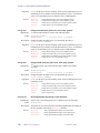
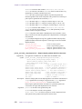
dres
Measure linewidth and digital resolution ...........................................
dsn
Measure signal-to-noise .....................................................................
dsnmax
Calculate maximum signal-to-noise ...................................................
getll
Get line frequency and intensity from line list ...................................
getreg
Get frequency limits of a specified region .........................................
integ
Find largest integral in specified region .............................................
mark
Determine intensity of the spectrum at a point ..................................
nll
Find line frequencies and intensities ..................................................
numreg
Return the number of regions in a spectrum ......................................
peak
Find tallest peak in specified region ..................................................
select
Select a spectrum or 2D plane without displaying it ..........................
Input/Output Tools ..........................................................................................................................
apa
Plot parameters automatically ............................................................
banner
Display message with large characters ..............................................
clear
Clear a window ..................................................................................
confirm
Confirm message using the mouse .....................................................
echo
Display strings and parameter values in text window ........................
flip
Flip between graphics and text window .............................................
format
Format a real number or convert a string for output ..........................
input
Receive input from keyboard .............................................................
lookup
Look up and return words and lines from text file .............................
nrecords
Determine number of lines in a file ....................................................
01-999165-00 A0800
VNMR 6.1C User Programming
5
25
26
26
28
28
29
29
32
33
34
35
35
36
36
37
37
38
38
38
38
38
38
38
39
39
39
39
39
39
40
40
40
40
40
40
40
40
41
41
41
Table of Contents
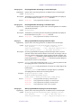
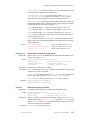
psgset
Set up parameters for various pulse sequences ..................................
vnmr_confirmer
Display a confirmer window (UNIX) ................................................
write
Write output to various devices .........................................................
Regression and Curve Fitting ..........................................................................................................
analyze
Generalized curve fitting ....................................................................
autoscale
Resume autoscaling after limits set by scalelimits .............................
expfit
Least-squares fit to exponential or polynomial curve (UNIX) ..........
expl
Display exponential or polynomial curves .........................................
pexpl
Plot exponential or polynomial curves ...............................................
poly0
Display mean of the data in the file regression.inp ............................
rinput
Input data for a regression analysis ....................................................
scalelimits
Set limits for scales in regression .......................................................
Mathematical Functions ..................................................................................................................
abs
Find absolute value of a number ........................................................
acos
Find arc cosine of a number ...............................................................
asin
Find arc sine of a number ...................................................................
atan
Find arc tangent of a number .............................................................
atan2
Find arc tangent of two numbers ........................................................
averag
Calculate average and standard deviation of input ............................
cos
Find cosine value of an angle .............................................................
exp
Find exponential value of a number ...................................................
ln
Find natural logarithm of a number ...................................................
sin
Find sine value of an angle ................................................................
tan
Find tangent value of an angle ...........................................................
Creating, Modifying, and Displaying Macros ................................................................................
crcom
Create a user macro without using a text editor .................................
delcom
Delete a user macro ............................................................................
hidecommand
Execute macro instead of command with same name .......................
macrocat
Display a user macro on the text window ..........................................
macrocp
Copy a user macro file .......................................................................
macrodir
List user macros .................................................................................
macroedit
Edit a user macro with user-selectable editor ....................................
macrold
Load a macro into memory ................................................................
macrorm
Remove a user macro .........................................................................
macrosyscat
Display a system macro on the text window ......................................
macrosyscp
Copy a system macro to become a user macro ..................................
macrosysdir
List system macros .............................................................................
macrosysrm
Remove a system macro ....................................................................
macrovi
Edit a user macro with vi text editor ..................................................
mstat
Display memory usage statistics ........................................................
purge
Remove a macro from memory .........................................................
record
Record keyboard entries as a macro ...................................................
Miscellaneous Tools ........................................................................................................................
axis
Provide axis labels and scaling factors ...............................................
beepoff
Turn beeper off ...................................................................................
beepon
Turn beeper on ...................................................................................
bootup
Macro executed automatically when VNMR is started .....................
exec
Execute a VNMR command ..............................................................
exists
Determine if a parameter, file, or macro exists ..................................
focus
Send keyboard focus to VNMR input window ..................................
gap
Find gap in the current spectrum ........................................................
getfile
Get information about directories and files ........................................
graphis
Return the current graphics display status .........................................
6
VNMR 6.1C User Programming
01-999165-00 A0800
41
41
41
42
42
42
42
42
42
42
42
42
43
43
43
43
43
43
43
43
43
43
44
44
44
44
44
44
44
44
44
44
45
45
45
45
45
45
45
45
45
46
46
46
46
46
46
46
46
47
47
47
47
Table of Contents
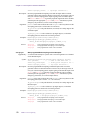
length
Determine length of a string ...............................................................
listenoff
Disable receipt of messages from send2Vnmr ...................................
listenon
Enable receipt of messages from send2Vnmr ....................................
login
User macro executed automatically when VNMR activated .............
off
Make a parameter inactive .................................................................
on
Make a parameter active or test its state ............................................
readlk
Read current lock level ......................................................................
rtv
Retrieve individual parameters ..........................................................
shell
Start a UNIX shell ..............................................................................
solppm
Return ppm and peak width of solvent resonances ............................
substr
Select a substring from a string ..........................................................
textis
Return the current text display status .................................................
unit
Define conversion units .....................................................................
1.4 Using Dialog Boxes from a Macro ..........................................................................................................
1.5 Customizing the Menu System ...............................................................................................................
Customizing the Permanent Menu ..................................................................................................
Customizing Menu Files and Help Files .........................................................................................
Controlling Menus ..........................................................................................................................
Programming Menus .......................................................................................................................
User-Programmable Menus in Interactive Programs ......................................................................
1.6 Customizing the Files Menus ..................................................................................................................
Starting the Program .......................................................................................................................
Selecting and Accessing Files .........................................................................................................
Using the Files Program with the Menu System ............................................................................
47
47
47
47
48
48
48
48
48
48
49
49
49
49
52
52
53
55
55
57
58
59
59
59
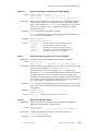
Chapter 2. Pulse Sequence Programming............................................................................ 63
2.1 Programming Pulse Sequences from Menus ...........................................................................................
Pulse Sequence Programming Menus .............................................................................................
Pulse Sequence Entry Main Menu ..................................................................................................
Pulse Sequence Entry Delay Menu .................................................................................................
Pulse Sequence Entry Phases Menu ...............................................................................................
Pulse Sequence Entry Phases Secondary Menu ..............................................................................
Pulse Sequence Entry Pulses Menu ................................................................................................
Pulse Sequence Entry Decoupler Pulses Menu ..............................................................................
Pulse Sequence Entry Status Menu .................................................................................................
2.2 Overview of Pulse Sequence Programming ............................................................................................
Spectrometer Differences ................................................................................................................
Pulse Sequence Generation Directory ............................................................................................
Compiling the New Pulse Sequence ...............................................................................................
Troubleshooting the New Pulse Sequence ......................................................................................
Types of Acquisition Controller Boards ..........................................................................................
Creating a Parameter Table for Pulse Sequence Object Code ........................................................
C Framework for Pulse Sequences .................................................................................................
Implicit Acquisition ........................................................................................................................
Acquisition Status Codes ................................................................................................................
2.3 Spectrometer Control ..............................................................................................................................
Creating a Time Delay ....................................................................................................................
Pulsing the Observe Transmitter .....................................................................................................
Pulsing the Decoupler Transmitter ..................................................................................................
Pulsing Channels Simultaneously ...................................................................................................
01-999165-00 A0800
VNMR 6.1C User Programming
7
63
65
66
66
67
67
67
68
68
69
69
69
70
71
72
72
72
74
74
79
79
80
82
84
Table of Contents
Setting Transmitter Quadrature Phase Shifts .................................................................................. 85
Setting Small-Angle Phase Shifts ................................................................................................... 86
Controlling the Offset Frequency ................................................................................................... 90
Controlling Observe and Decoupler Transmitter Power ................................................................. 91
Controlling Status and Gating ......................................................................................................... 93
Interfacing to External User Devices .............................................................................................. 97
2.4 Pulse Sequence Statements: Phase and Sequence Control ...................................................................... 98
Real-Time Variables and Constants ................................................................................................ 98
Calculating in Real-Time Using Integer Mathematics .................................................................... 99
Controlling a Sequence Using Real-Time Variables ..................................................................... 100
Real-Time vs. Run-Time—When Do Things Happen? ................................................................ 101
Manipulating Acquisition Variables .............................................................................................. 102
Intertransient and Interincrement Delays ...................................................................................... 103
Controlling Pulse Sequence Graphical Display ............................................................................ 104
2.5 Real-Time AP Tables ............................................................................................................................. 104
Loading AP Table Statements from UNIX Text Files ................................................................... 105
Table Names and Statements ........................................................................................................ 105
AP Table Notation ......................................................................................................................... 106
Handling AP Tables ...................................................................................................................... 107
Examples of Using AP Tables ....................................................................................................... 108
2.6 Accessing Parameters ............................................................................................................................ 110
Categories of Parameters .............................................................................................................. 110
Looking Up Parameter Values ...................................................................................................... 117
Using Parameters in a Pulse Sequence ......................................................................................... 117
2.7 Using Interactive Parameter Adjustment ............................................................................................... 120
General Routines ........................................................................................................................... 120
Generic Pulse Routine ................................................................................................................... 121
Frequency Offset Subroutine ........................................................................................................ 122
Generic Delay Routine .................................................................................................................. 123
Fine Power Subroutine .................................................................................................................. 125
2.8 Hardware Looping and Explicit Acquisition ......................................................................................... 125
Controlling Hardware Looping ..................................................................................................... 126
Number of Events in Hardware Loops ......................................................................................... 127
Explicit Acquisition ...................................................................................................................... 129
Receiver Phase For Explicit Acquisitions ..................................................................................... 130
Multiple FID Acquisition .............................................................................................................. 130
2.9 Pulse Sequence Synchronization ........................................................................................................... 131
External Time Base ....................................................................................................................... 131
Controlling Rotor Synchronization ............................................................................................... 131
2.10 Pulse Shaping ...................................................................................................................................... 131
File Specifications ......................................................................................................................... 132
Performing Shaped Pulses ............................................................................................................ 134
Programmable Transmitter Control .............................................................................................. 136
Setting Spin Lock Waveform Control ........................................................................................... 137
Shaped Pulse Calibration .............................................................................................................. 138
2.11 Shaped Pulses Using Attenuators ........................................................................................................ 138
AP Bus Delay Constants ............................................................................................................... 139
Controlling Shaped Pulses Using Attenuators .............................................................................. 140
Controlling Attenuation ................................................................................................................ 141
8
VNMR 6.1C User Programming
01-999165-00 A0800
Table of Contents
2.12 Internal Hardware Delays ....................................................................................................................
Delays from Changing Attenuation ..............................................................................................
Delays from Changing Status .......................................................................................................
Waveform Generator High-Speed Line Trigger ............................................................................
2.13 Indirect Detection on Fixed-Frequency Channel ................................................................................
Fixed-Frequency Decoupler ..........................................................................................................
2.14 Multidimensional NMR ......................................................................................................................
Hypercomplex 2D .........................................................................................................................
Real Mode Phased 2D: TPPI ........................................................................................................
2.15 Gradient Control for PFG and Imaging ...............................................................................................
Setting the Gradient Current Amplifier Level ...............................................................................
Generating a Gradient Pulse .........................................................................................................
Controlling Lock Correction Circuitry .........................................................................................
Programming Microimaging Pulse Sequences .............................................................................
2.16 Programming the Performa XYZ PFG Module ..................................................................................
Creating Gradient Tables ..............................................................................................................
Pulse Sequence Programming .......................................................................................................
2.17 Imaging-Related Statements ...............................................................................................................
Real-time Gradient Statements .....................................................................................................
Oblique Gradient Statements ........................................................................................................
Global List and Position Statements .............................................................................................
Looping Statements ......................................................................................................................
Waveform Initialization Statements ..............................................................................................
Other Statements ...........................................................................................................................
2.18 User-Customized Pulse Sequence Generation ....................................................................................
142
143
143
145
146
146
148
148
150
150
150
151
151
152
153
153
154
155
155
155
157
157
157
157
157
Chapter 3. Pulse Sequence Statement Reference ............................................................. 159
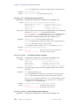
acquire
add
apovrride
apshaped_decpulse
apshaped_dec2pulse
apshaped_pulse
assign
blankingoff
blankingon
blankoff
blankon
clearapdatatable
create_delay_list
create_freq_list
create_offset_list
dbl
dcphase
dcplrphase
dcplr2phase
dcplr3phase
decblank
dec2blank
dec3blank
declvloff
01-999165-00 A0800
Explicitly acquire data .......................................................................159
Add integer values ..............................................................................160
Override internal software AP bus delay ............................................160
First decoupler pulse shaping via AP bus ..........................................161
Second decoupler pulse shaping via AP bus ......................................162
Observe transmitter pulse shaping via AP bus ...................................163
Assign integer values .........................................................................164
Unblank amplifier channels and turn amplifiers on ...........................164
Blank amplifier channels and turn amplifiers off ...............................164
Stop blanking observe or decoupler amplifier (obsolete) ..................164
Start blanking observe or decoupler amplifier (obsolete) ..................165
Zero all data in acquisition processor memory ..................................165
Create table of delays .........................................................................165
Create table of frequencies .................................................................166
Create table of frequency offsets ........................................................167
Double an integer value ......................................................................168
Set decoupler phase (obsolete) ...........................................................168
Set small-angle phase of 1st decoupler, rf type C or D ......................169
Set small-angle phase of 2nd decoupler, rf type C or D ....................169
Set small-angle phase of 3rd decoupler, rf type C or D .....................170
Blank amplifier associated with first decoupler .................................170
Blank amplifier associated with second decoupler ............................170
Blank amplifier associated with third decoupler ................................171
Return first decoupler back to “normal” power .................................171
VNMR 6.1C User Programming
9
Table of Contents
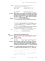
declvlon
decoff
dec2off
dec3off
decoffset
dec2offset
dec3offset
dec4offset
decon
dec2on
dec3on
decphase
dec2phase
dec3phase
dec4phase
decpower
dec2power
dec3power
dec4power
decprgoff
dec2prgoff
dec3prgoff
decprgon
dec2prgon
dec3prgon
decpulse
decpwr
decpwrf
dec2pwrf
dec3pwrf
decr
decrgpulse
dec2rgpulse
dec3rgpulse
dec4rgpulse
decshaped_pulse
dec2shaped_pulse
dec3shaped_pulse
decspinlock
dec2spinlock
dec3spinlock
decstepsize
dec2stepsize
dec3stepsize
decunblank
dec2unblank
dec3unblank
delay
dhpflag
divn
dps_off
dps_on
dps_show
dps_skip
10
VNMR 6.1C User Programming
Turn on first decoupler to full power ..................................................171
Turn off first decoupler .......................................................................172
Turn off second decoupler ..................................................................172
Turn off third decoupler .....................................................................172
Change offset frequency of first decoupler ........................................172
Change offset frequency of second decoupler ...................................172
Change offset frequency of third decoupler .......................................173
Change offset frequency of fourth decoupler .....................................173
Turn on first decoupler .......................................................................173
Turn on second decoupler ..................................................................173
Turn on third decoupler ......................................................................174
Set quadrature phase of first decoupler ..............................................174
Set quadrature phase of second decoupler .........................................174
Set quadrature phase of third decoupler .............................................174
Set quadrature phase of fourth decoupler ...........................................175
Change first decoupler power level, linear amp. systems ..................175
Change second decoupler power level, linear amp. systems .............175
Change third decoupler power level, linear amp. systems .................176
Change fourth decoupler power level, linear amp. systems ...............176
End programmable decoupling on first decoupler .............................176
End programmable decoupling on second decoupler ........................177
End programmable decoupling on third decoupler ............................177
Start programmable decoupling on first decoupler ............................177
Start programmable decoupling on second decoupler .......................177
Start programmable decoupling on third decoupler ...........................178
Pulse first decoupler transmitter with amplifier gating ......................179
Set first decoupler high-power level, class C amplifier ......................179
Set first decoupler fine power .............................................................179
Set second decoupler fine power ........................................................180
Set third decoupler fine power ...........................................................180
Decrement an integer value ................................................................180
Pulse first decoupler with amplifier gating .........................................181
Pulse second decoupler with amplifier gating ....................................182
Pulse third decoupler with amplifier gating .......................................182
Pulse fourth decoupler with amplifier gating .....................................183
Perform shaped pulse on first decoupler ............................................183
Perform shaped pulse on second decoupler .......................................184
Perform shaped pulse on third decoupler ...........................................185
Set spin lock waveform control on first decoupler .............................186
Set spin lock waveform control on second decoupler ........................187
Set spin lock waveform control on third decoupler ...........................187
Set step size for first decoupler ..........................................................188
Set step size for second decoupler .....................................................188
Set step size for third decoupler .........................................................189
Unblank amplifier associated with first decoupler .............................189
Unblank amplifier associated with second decoupler ........................189
Unblank amplifier associated with third decoupler ............................189
Delay for a specified time ..................................................................190
Switch decoupling from low-power to high-power ...........................190
Divide integer values ..........................................................................190
Turn off graphical display of statements ............................................190
Turn on graphical display of statements ............................................191
Draw delay or pulses in a sequence for graphical display .................191
Skip graphical display of next statement ...........................................193
01-999165-00 A0800
Table of Contents
elsenz
endhardloop
endif
endloop
endmsloop
endpeloop
gate
getarray
getelem
getorientation
getstr
getval
G_Delay
G_Offset
G_Power
G_Pulse
hdwshiminit
hlv
hsdelay
idecpulse
idecrgpulse
idelay
ifzero
incdelay
incgradient
incr
indirect
init_rfpattern
init_gradpattern
init_vscan
initdelay
initparms_sis
initval
iobspulse
ioffset
ipulse
ipwrf
ipwrm
irgpulse
lk_hold
lk_sample
loadtable
loop
magradient
magradpulse
mashapedgradient
mashapedgradpulse
mod2
mod4
modn
msloop
mult
obl_gradient
oblique_gradient
01-999165-00 A0800
Execute succeeding statements if argument is nonzero .....................193
End hardware loop .............................................................................194
End execution started by ifzero or elsenz ...........................................194
End loop .............................................................................................194
End multislice loop ............................................................................195
End phase-encode loop ......................................................................195
Device gating (obsolete) .....................................................................196
Get arrayed parameter values .............................................................196
Retrieve an element from an AP table ................................................197
Read image plane orientation .............................................................197
Look up value of string parameter .....................................................198
Look up value of numeric parameter .................................................198
Generic delay routine .........................................................................199
Frequency offset routine .....................................................................199
Fine power routine .............................................................................199
Generic pulse routine .........................................................................199
Initialize next delay for hardware shimming .....................................200
Find half the value of an integer .........................................................200
Delay specified time with possible homospoil pulse .........................201
Pulse first decoupler transmitter with IPA ..........................................201
Pulse first decoupler with amplifier gating and IPA ...........................202
Delay for a specified time with IPA ...................................................202
Execute succeeding statements if argument is zero ..........................202
Set real-time incremental delay ..........................................................203
Generate dynamic variable gradient pulse .........................................203
Increment an integer value .................................................................204
Set indirect detection ..........................................................................205
Create rf pattern file ...........................................................................205
Create gradient pattern file .................................................................206
Initialize real-time variable for vscan statement ................................207
Initialize incremental delay ................................................................207
Initialize parameters for spectroscopy imaging sequences ................207
Initialize a real-time variable to specified value .................................208
Pulse observe transmitter with IPA ....................................................208
Change offset frequency with IPA .....................................................208
Pulse observe transmitter with IPA ....................................................209
Change transmitter or decoupler fine power with IPA .......................209
Change transmitter or decoupler lin. mod. power with IPA ...............210
Pulse observe transmitter with IPA ....................................................210
Set lock correction circuitry to hold correction ..................................211
Set lock correction circuitry to sample lock signal ............................211
Load AP table elements from table text file .......................................211
Start loop ............................................................................................212
Simultaneous gradient at the magic angle ..........................................212
Gradient pulse at the magic angle ......................................................213
Simultaneous shaped gradient at the magic angle ..............................213
Simultaneous shaped gradient pulse at the magic angle ....................214
Find integer value modulo 2 ...............................................................215
Find integer value modulo 4 ...............................................................215
Find integer value modulo n ...............................................................216
Multislice loop ...................................................................................216
Multiply integer values .......................................................................217
Execute an oblique gradient ...............................................................217
Execute an oblique gradient ...............................................................218
VNMR 6.1C User Programming
11
Table of Contents
obl_shapedgradient
oblique_shapedgradient
obsblank
obsoffset
obspower
obsprgoff
obsprgon
obspulse
obspwrf
obsstepsize
obsunblank
offset
pe_gradient
pe2_gradient
pe3_gradient
pe_shapedgradient
pe2_shapedgradient
pe3_shapedgradient
peloop
phase_encode_gradient
phase_encode3_gradient
phase_encode_shapedgradient
phase_encode3_shapedgradient
phaseshift
poffset
poffset_list
position_offset
position_offset_list
power
pulse
pwrf
pwrm
rcvroff
rcvron
readuserap
recoff
recon
rgpulse
rgradient
rlpower
rlpwrf
rlpwrm
rotorperiod
rotorsync
setautoincrement
setdivnfactor
setreceiver
setstatus
settable
setuserap
shapedpulse
shaped_pulse
shapedgradient
shaped2Dgradient
12
VNMR 6.1C User Programming
Execute a shaped oblique gradient .....................................................218
Execute a shaped oblique gradient .....................................................219
Blank amplifier associated with observe transmitter .........................220
Change offset frequency of observe transmitter .................................220
Change observe transmitter power level, lin. amp. systems ..............221
End programmable control of observe transmitter .............................221
Start programmable control of observe transmitter ...........................221
Pulse observe transmitter with amplifier gating .................................222
Set observe transmitter fine power .....................................................222
Set step size for observe transmitter ...................................................222
Unblank amplifier associated with observe transmitter .....................223
Change offset frequency of transmitter or decoupler .........................223
Oblique gradient with phase encode in one axis ................................223
Oblique gradient with phase encode in two axes ...............................224
Oblique gradient with phase encode in three axes .............................224
Oblique shaped gradient with phase encode in one axis ....................225
Oblique shaped gradient with phase encode in two axes ...................226
Oblique shaped gradient with phase encode in three axes .................226
Phase-encode loop ..............................................................................227
Oblique gradient with phase encode in one axis ................................228
Oblique gradient with phase encode in three axes .............................228
Oblique shaped gradient with PE in one axis ....................................229
Oblique shaped gradient with PE in three axes ..................................230
Set phase-pulse technique, rf type A or B ..........................................231
Set frequency based on position .........................................................231
Set frequency from position list .........................................................232
Set frequency based on position .........................................................232
Set frequency from position list .........................................................232
Change power level, linear amplifier systems ....................................233
Pulse observe transmitter with amplifier gating .................................234
Change transmitter or decoupler fine power ......................................234
Change transmitter or decoupler linear modulator power ..................235
Turn off receiver gate and amplifier blanking gate ............................235
Turn on receiver gate and amplifier blanking gate .............................236
Read input from user AP register .......................................................236
Turn off receiver gate only .................................................................237
Turn on receiver gate only ..................................................................237
Pulse observe transmitter with amplifier gating .................................238
Set gradient to specified level .............................................................238
Change power level, linear amplifier systems ....................................239
Set transmitter or decoupler fine power .............................................240
Set transmitter or decoupler linear modulator power .........................240
Obtain rotor period of MAS rotor ......................................................240
Gated pulse sequence delay from MAS rotor position ......................241
Set autoincrement attribute for an AP table .......................................241
Set divn-return attribute and divn-factor for AP table ........................242
Associate the receiver phase cycle with an AP table ..........................242
Set status of observe transmitter or decoupler transmitter .................242
Store an array of integers in a real-time AP table ..............................243
Set user AP register ............................................................................244
Perform shaped pulse on observe transmitter ....................................244
Perform shaped pulse on observe transmitter ....................................244
Generate shaped gradient pulse .......................................................245
Generate arrayed shaped gradient pulse .............................................246
01-999165-00 A0800
Table of Contents
shapedincgradient
shapedvgradient
simpulse
sim3pulse
sim4pulse
simshaped_pulse
sim3shaped_pulse
sli
sp#off
sp#on
spinlock
starthardloop
status
statusdelay
stepsize
sub
tsadd
tsdiv
tsmult
tssub
ttadd
ttdiv
ttmult
ttsub
txphase
vagradient
vagradpulse
vashapedgradient
vashapedgradpulse
vdelay
vdelay_list
vfreq
vgradient
voffset
vscan
vsetuserap
vsli
xgate
xmtroff
xmtron
xmtrphase
zero_all_gradients
zgradpulse
Generate dynamic variable gradient pulse .........................................248
Generate dynamic variable shaped gradient pulse .............................249
Pulse observe and decouple channels simultaneously .......................251
Pulse simultaneously on 2 or 3 rf channels ........................................251
Simultaneous pulse on four channels .................................................252
Perform simultaneous two-pulse shaped pulse ..................................253
Perform a simultaneous three-pulse shaped pulse .............................254
Set SLI lines .......................................................................................255
Turn off specified spare line ...............................................................256
Turn on specified spare line ...............................................................257
Control spin lock on observe transmitter ...........................................257
Start hardware loop ............................................................................258
Change status of decoupler and homospoil ........................................259
Execute the status statement with a given delay time ........................259
Set small-angle phase step size, rf type C or D ..................................260
Subtract integer values .......................................................................261
Add an integer to AP table elements ..................................................261
Divide an integer into AP table elements ...........................................262
Multiply an integer with AP table elements .......................................262
Subtract an integer from AP table elements .......................................263
Add an AP table to a second table ......................................................263
Divide an AP table into a second table ...............................................263
Multiply an AP table by a second table ..............................................264
Subtract an AP table from a second table ...........................................264
Set quadrature phase of observe transmitter ......................................265
Variable angle gradient .......................................................................265
Variable angle gradient pulse .............................................................266
Variable angle shaped gradient ...........................................................266
Variable angle shaped gradient pulse .................................................268
Set delay with fixed timebase and real-time count .............................268
Get delay value from delay list with real-time index .........................269
Select frequency from table ...............................................................270
Set gradient to a level determined by real-time math .........................270
Select frequency offset from table .....................................................272
Provide dynamic variable scan ...........................................................272
Set user AP register using real-time variable .....................................273
Set SLI lines from real-time variable .................................................273
Gate pulse sequence from an external event ......................................275
Turn off observe transmitter ...............................................................275
Turn on observe transmitter ...............................................................275
Set transmitter small-angle phase, rf type C, D .................................275
Zero all gradients ...............................................................................276
Create a gradient pulse on the z channel ............................................276
Chapter 4. UNIX-Level Programming .................................................................................. 277
4.1 UNIX and VNMR .................................................................................................................................
4.2 UNIX: A Reference Guide ....................................................................................................................
Command Entry ............................................................................................................................
File Names ...................................................................................................................................
File Handling Commands .............................................................................................................
Directory Names ..........................................................................................................................
Directory Handling Commands ....................................................................................................
Text Commands ............................................................................................................................
01-999165-00 A0800
VNMR 6.1C User Programming
13
277
278
278
278
278
278
278
279
Table of Contents
Other Commands .........................................................................................................................
Special Characters .........................................................................................................................
4.3 UNIX Commands Accessible from VNMR ..........................................................................................
Opening a UNIX Text Editor from VNMR ..................................................................................
Opening a UNIX Shell from VNMR ............................................................................................
4.4 Background VNMR ...............................................................................................................................
Running VNMR Command as a UNIX Background Task ...........................................................
Running VNMR Processing in the Background ...........................................................................
4.5 Shell Programming ................................................................................................................................
Shell Variables and Control Formats .............................................................................................
Shell Scripts ..................................................................................................................................
279
279
280
280
280
280
281
281
282
282
282
Chapter 5. Parameters and Data .......................................................................................... 283
5.1 VNMR Data Files ..................................................................................................................................
Binary Data Files ..........................................................................................................................
Data File Structures .......................................................................................................................
VNMR Use of Binary Data Files ..................................................................................................
Storing Multiple Traces .................................................................................................................
Header and Data Display ..............................................................................................................
5.2 FDF (Flexible Data Format) Files .........................................................................................................
File Structures and Naming Conventions .....................................................................................
File Format ....................................................................................................................................
Header Parameters ........................................................................................................................
Transformations ............................................................................................................................
Creating FDF Files ........................................................................................................................
Splitting FDF Files ........................................................................................................................
5.3 Reformatting Data for Processing .........................................................................................................
Standard and Compressed Formats ...............................................................................................
Compress or Uncompress Data .....................................................................................................
Move and Reverse Data ................................................................................................................
Table Convert Data ........................................................................................................................
Reformatting Spectra ....................................................................................................................
5.4 Creating and Modifying Parameters ......................................................................................................
Parameter Types and Trees ............................................................................................................
Tools for Working with Parameter Trees ......................................................................................
Format of a Stored Parameter .......................................................................................................
5.5 Modifying Parameter Displays in VNMR .............................................................................................
Display Template ..........................................................................................................................
Default Display Templates ............................................................................................................
Conditional and Arrayed Displays ................................................................................................
Output Format ...............................................................................................................................
5.6 User-Written Weighting Functions ........................................................................................................
Writing a Weighting Function .......................................................................................................
Compiling the Weighting Function ...............................................................................................
5.7 User-Written FID Files ..........................................................................................................................
283
283
285
288
289
290
290
290
291
291
294
294
295
295
295
296
296
298
298
298
298
299
301
304
304
305
306
307
307
308
309
310
Chapter 6. Customizing Graphics Windows ....................................................................... 311
6.1 Customizing the Sample Entry Form Window ...................................................................................... 311
Window Configuration Files ......................................................................................................... 311
Setting Which Selections Are Displayed ...................................................................................... 314
14
VNMR 6.1C User Programming
01-999165-00 A0800
Table of Contents
Setting the Content of the Output File ..........................................................................................
Setting Name Attributes ................................................................................................................
Setting the Types of Widgets .........................................................................................................
Alternate Interfaces .......................................................................................................................
File Attribute .................................................................................................................................
Button Definitions .........................................................................................................................
Sample Entry Control ...................................................................................................................
Adding a New Field ......................................................................................................................
6.2 Customizing the status Window ............................................................................................................
Window Configuration File ...........................................................................................................
Defining Buttons and Window Attributes .....................................................................................
6.3 Customizing the Interactive dg Window ...............................................................................................
Types of Fields ..............................................................................................................................
Selecting the New Interface ..........................................................................................................
Deselecting the New Interface ......................................................................................................
Window Configuration Files .........................................................................................................
Editing the Configuration Files .....................................................................................................
Interaction Elements .....................................................................................................................
Tips for dg Design .........................................................................................................................
Utilities for Accessing VNMR Parameters. ..................................................................................
Sending a Tcl Script ......................................................................................................................
314
315
316
316
317
319
321
322
322
323
324
324
326
328
328
328
328
332
339
342
343
Index........................................................................................................................................ 345
01-999165-00 A0800
VNMR 6.1C User Programming
15
Table of Contents
16
VNMR 6.1C User Programming
01-999165-00 A0800
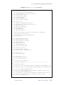
List of Figures
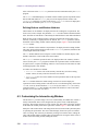
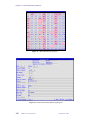
Figure 1. Dialog Box for array Macro ....................................................................................... 50
Figure 2. Homonuclear-2D-J Pulse Sequence ............................................................................... 64
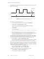
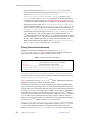
Figure 3. Amplifier Gating ............................................................................................................. 81
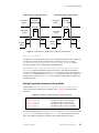
Figure 4. Pulse Observe and Decoupler Channels Simultaneously ............................................... 85
Figure 5. Waveform Generator Offset Delay on UNITYINOVA Systems ........................................ 145
Figure 6. Magnet Coordinates as Related to User Coordinates. .................................................. 292
Figure 7. Single-String Display Template with Output ............................................................... 304
Figure 8. Multiple-String Display Template ................................................................................ 305
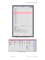
Figure 9. Default Interface (enter Program) ................................................................................ 315
Figure 10. Alternate Interface (enter Program) ............................................................................ 317
Figure 11. Second Alternate Interface (enter Program) ............................................................... 318
Figure 12. Default Interface (status Program) ............................................................................. 325
Figure 13. dg Window ................................................................................................................. 325
Figure 14. Matrix Window (dg Program) .................................................................................... 330
Figure 15. Interaction Elements Window (dg Program) .............................................................. 330
01-999165-00 A0800
VNMR 6.1C User Programming
17
List of Tables
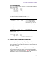
Table 1. Reserved Words in MAGICAL. ....................................................................................... 30
Table 2. Order of Operator Precedence (Highest First) in MAGICAL ......................................... 31
Table 3. Menu-Related Commands and Parameters ...................................................................... 52
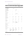
Table 4. Variable Types in Pulse Sequences .................................................................................. 74
Table 5. Acquisition Status Codes ................................................................................................. 75
Table 6. Delay-Related Statements ................................................................................................ 79
Table 7. Observe Transmitter Pulse-Related Statements ............................................................... 81
Table 8. Decoupler Transmitter Pulse-Related Statements ............................................................ 83
Table 9. Simultaneous Pulses Statements ...................................................................................... 84
Table 10. Transmitter Quadrature Phase Control Statements ........................................................ 85
Table 11. Phase Shift Statements ................................................................................................... 86
Table 12. Frequency Control Statements ....................................................................................... 90
Table 13. Power Control Statements .............................................................................................. 91
Table 14. Gating Control Statements ............................................................................................. 94
Table 15. Interfacing to External User Devices ............................................................................. 97
Table 16. Mapping of User AP Lines ............................................................................................ 97
Table 17. Integer Mathematics Statements .................................................................................... 99
Table 18. Pulse Sequence Control Statements ............................................................................. 100
Table 19. Statements for Controlling Graphical Display of a Sequence ..................................... 104
Table 20. Statements for Handling AP Tables ............................................................................. 107
Table 21. Parameter Value Lookup Statements ........................................................................... 110
Table 22. Global PSG Parameters ................................................................................................ 111
Table 23. Imaging Variables ......................................................................................................... 113
Table 24. Hardware Looping Related Statements ....................................................................... 126
Table 25. Number of Events for Statements in a Hardware Loop ............................................... 128
Table 26. Rotor Synchronization Control Statements ................................................................. 131
Table 27. Shaped Pulse Statements .............................................................................................. 134
Table 28. Programmable Control Statements .............................................................................. 137
Table 29. Spin Lock Control Statements ..................................................................................... 138
Table 30. AP Bus Delay Constants ............................................................................................. 140
Table 31. Statements for Pulse Shaping Through the AP Bus ..................................................... 141
Table 32. AP Bus Overhead Delays ............................................................................................. 144
Table 33. Example of AP Bus Overhead Delays for status Statement ................................... 145
Table 34. Multidimensional PSG Variables ................................................................................. 149
Table 35. Gradient Control Statements ........................................................................................ 151
Table 36. Delays for Obliquing and Shaped Gradient Statements .............................................. 152
Table 37. Performa XYZ PFG Module Statements ..................................................................... 154
Table 38. Imaging-Related Statements ........................................................................................ 156
Table 39. Commands for Reformatting Data .............................................................................. 296
Table 40. Commands for Working with Parameter Trees ............................................................ 300
18
VNMR 6.1C User Programming
01-999165-00 A0800
SAFETY PRECAUTIONS
The following warning and caution notices illustrate the style used in Varian manuals for
safety precaution notices and explain when each type is used:
WARNING: Warnings are used when failure to observe instructions or precautions
could result in injury or death to humans or animals, or significant
property damage.
CAUTION:
Cautions are used when failure to observe instructions could result in
serious damage to equipment or loss of data.
Warning Notices
Observe the following precautions during installation, operation, maintenance, and repair
of the instrument. Failure to comply with these warnings, or with specific warnings
elsewhere in Varian manuals, violates safety standards of design, manufacturing, and
intended use of the instrument. Varian assumes no liability for customer failure to comply
with these precautions.
WARNING: Persons with implanted or attached medical devices such as
pacemakers and prosthetic parts must remain outside the 5-gauss
perimeter from the centerline of the magnet.
The superconducting magnet system generates strong magnetic fields that can
affect operation of some cardiac pacemakers or harm implanted or attached
devices such as prosthetic parts and metal blood vessel clips and clamps.
Pacemaker wearers should consult the user manual provided by the pacemaker
manufacturer or contact the pacemaker manufacturer to determine the effect on
a specific pacemaker. Pacemaker wearers should also always notify their
physician and discuss the health risks of being in proximity to magnetic fields.
Wearers of metal prosthetics and implants should contact their physician to
determine if a danger exists.
Refer to the manuals supplied with the magnet for the size of a typical 5-gauss
stray field. This gauss level should be checked after the magnet is installed.
WARNING: Keep metal objects outside the 10-gauss perimeter from the centerline
of the magnet.
The strong magnetic field surrounding the magnet attracts objects containing
steel, iron, or other ferromagnetic materials, which includes most ordinary
tools, electronic equipment, compressed gas cylinders, steel chairs, and steel
carts. Unless restrained, such objects can suddenly fly towards the magnet,
causing possible personal injury and extensive damage to the probe, dewar, and
superconducting solenoid. The greater the mass of the object, the more the
magnet attracts the object.
Only nonferromagnetic materials—plastics, aluminum, wood, nonmagnetic
stainless steel, etc.—should be used in the area around the magnet. If an object
is stuck to the magnet surface and cannot easily be removed by hand, contact
Varian service for assistance.
01-999165-00 A0800
VNMR 6.1C User Programming
19
SAFETY PRECAUTIONS
Warning Notices (continued)
Refer to the manuals supplied with the magnet for the size of a typical 10-gauss
stray field. This gauss level should be checked after the magnet is installed.
WARNING: Only qualified maintenance personnel shall remove equipment covers
or make internal adjustments.
Dangerous high voltages that can kill or injure exist inside the instrument.
Before working inside a cabinet, turn off the main system power switch located
on the back of the console, then disconnect the ac power cord.
WARNING: Do not substitute parts or modify the instrument.
Any unauthorized modification could injure personnel or damage equipment
and potentially terminate the warranty agreements and/or service contract.
Written authorization approved by a Varian, Inc. product manager is required to
implement any changes to the hardware of a Varian NMR spectrometer.
Maintain safety features by referring system service to a Varian service office.
WARNING: Do not operate in the presence of flammable gases or fumes.
Operation with flammable gases or fumes present creates the risk of injury or
death from toxic fumes, explosion, or fire.
WARNING: Leave area immediately in the event of a magnet quench.
If the magnet dewar should quench (sudden appearance of gasses from the top
of the dewar), leave the area immediately. Sudden release of helium or nitrogen
gases can rapidly displace oxygen in an enclosed space creating a possibility of
asphyxiation. Do not return until the oxygen level returns to normal.
WARNING: Avoid liquid helium or nitrogen contact with any part of the body.
In contact with the body, liquid helium and nitrogen can cause an injury similar
to a burn. Never place your head over the helium and nitrogen exit tubes on top
of the magnet. If liquid helium or nitrogen contacts the body, seek immediate
medical attention, especially if the skin is blistered or the eyes are affected.
WARNING: Do not look down the upper barrel.
Unless the probe is removed from the magnet, never look down the upper
barrel. You could be injured by the sample tube as it ejects pneumatically from
the probe.
WARNING: Do not exceed the boiling or freezing point of a sample during variable
temperature experiments.
A sample tube subjected to a change in temperature can build up excessive
pressure, which can break the sample tube glass and cause injury by flying glass
and toxic materials. To avoid this hazard, establish the freezing and boiling
point of a sample before doing a variable temperature experiment.
20
VNMR 6.1C User Programming
01-999165-00 A0800
SAFETY PRECAUTIONS
Warning Notices (continued)
WARNING: Support the magnet and prevent it from tipping over.
The magnet dewar has a high center of gravity and could tip over in an
earthquake or after being struck by a large object, injuring personnel and
causing sudden, dangerous release of nitrogen and helium gasses from the
dewar. Therefore, the magnet must be supported by at least one of two methods:
with ropes suspended from the ceiling or with the antivibration legs bolted to
the floor. Refer to the Installation Planning Manual for details.
WARNING: Do not remove the relief valves on the vent tubes.
The relief valves prevent air from entering the nitrogen and helium vent tubes.
Air that enters the magnet contains moisture that can freeze, causing blockage
of the vent tubes and possibly extensive damage to the magnet. It could also
cause a sudden dangerous release of nitrogen and helium gases from the dewar.
Except when transferring nitrogen or helium, be certain that the relief valves are
secured on the vent tubes.
WARNING: On magnets with removable quench tubes, keep the tubes in place
except during helium servicing.
On Varian 200- and 300-MHz 54-mm magnets only, the dewar includes
removable helium vent tubes. If the magnet dewar should quench (sudden
appearance of gases from the top of the dewar) and the vent tubes are not in
place, the helium gas would be partially vented sideways, possibly injuring the
skin and eyes of personnel beside the magnet. During helium servicing, when
the tubes must be removed, carefully follow the instructions and safety
precautions given in the manual supplied with the magnet.
Caution Notices
Observe the following precautions during installation, operation, maintenance, and repair
of the instrument. Failure to comply with these cautions, or with specific cautions elsewhere
in Varian manuals, violates safety standards of design, manufacturing, and intended use of
the instrument. Varian assumes no liability for customer failure to comply with these
precautions.
CAUTION:
Keep magnetic media, ATM and credit cards, and watches outside the
5-gauss perimeter from the centerline of the magnet.
The strong magnetic field surrounding a superconducting magnet can erase
magnetic media such as floppy disks and tapes. The field can also damage the
strip of magnetic media found on credit cards, automatic teller machine (ATM)
cards, and similar plastic cards. Many wrist and pocket watches are also
susceptible to damage from intense magnetism.
Refer to the manuals supplied with the magnet for the size of a typical 5-gauss
stray field. This gauss level should be checked after the magnet is installed.
01-999165-00 A0800
VNMR 6.1C User Programming
21
SAFETY PRECAUTIONS
Caution Notices (continued)
CAUTION:
Keep the PCs, (including the LC STAR workstation) beyond the 5gauss perimeter of the magnet.
Avoid equipment damage or data loss by keeping PCs (including the LC
workstation PC) well away from the magnet. Generally, keep the PC beyond the
5-gauss perimeter of the magnet. Refer to the Installation Planning Guide for
magnet field plots.
CAUTION:
Check helium and nitrogen gas flowmeters daily.
Record the readings to establish the operating level. The readings will vary
somewhat because of changes in barometric pressure from weather fronts. If
the readings for either gas should change abruptly, contact qualified
maintenance personnel. Failure to correct the cause of abnormal readings could
result in extensive equipment damage.
CAUTION:
Never operate solids high-power amplifiers with liquids probes.
On systems with solids high-power amplifiers, never operate the amplifiers
with a liquids probe. The high power available from these amplifiers will
destroy liquids probes. Use the appropriate high-power probe with the highpower amplifier.
CAUTION:
Take electrostatic discharge (ESD) precautions to avoid damage to
sensitive electronic components.
Wear a grounded antistatic wristband or equivalent before touching any parts
inside the doors and covers of the spectrometer system. Also, take ESD
precautions when working near the exposed cable connectors on the back of the
console.
Radio-Frequency Emission Regulations
The covers on the instrument form a barrier to radio-frequency (rf) energy. Removing any
of the covers or modifying the instrument may lead to increased susceptibility to rf
interference within the instrument and may increase the rf energy transmitted by the
instrument in violation of regulations covering rf emissions. It is the operator’s
responsibility to maintain the instrument in a condition that does not violate rf emission
requirements.
22
VNMR 6.1C User Programming
01-999165-00 A0800
Introduction
Varian's VNMR software provides NMR users with an exceptionally responsive user
programming environment that allows customizing the system software and the operator
interface. This manual explains how to use these capabilities:
• Chapter 1, “MAGICAL II Programming,” describes MAGICAL II (MAGnetics
Instrument Control and Analysis Language), a powerful software application that
enables full automation of spectrometer operation and data analysis using macros.
• Chapter 2, “Pulse Sequence Programming,” covers pulse sequence programming, via
menus as well as user-written programs, using Varian’s powerful and extensive set of
pulse sequence statements.
• Chapter 3, “Pulse Sequence Statement Reference,” is an alphabetical reference to each
pulse sequence statement in VNMR.
• Chapter 4, “UNIX-Level Programming,” is a short overview of UNIX, the operating
system used with VNMR.
• Chapter 5, “Parameters and Data,” covers manipulating parameters, using data files,
modifying parameter displays, and writing user-defined weighting functions
• Chapter 6, “Customizing Graphics Windows,” describes how to customize the
interactive graphics display windows for the enter, status, and dg programs.
Notational Conventions
The following notational conventions are used throughout all VNMR manuals:
• Typewriter-like characters identify VNMR and UNIX commands,
parameters, directories, and file names in the text of the manual. For example:
The shutdown command is in the /etc directory.
• Typewriter-like characters also show text displayed on the screen,
including the text echoed on the screen as you enter commands. For example:
Self test completed successfully.
• Text shown between angled brackets (<...>) in a syntax entry is optional. For example,
if the syntax is seqgen s2pul<.c>, entering the “.c” suffix is optional, and typing
seqgen s2pul.c or seqgen s2pul is functionally the same.
• Lines of text containing command syntax, examples of statements, source code, and
similar material are often too long to fit the width of the page. To show that a line of
text had to be broken to fit into the manual, the line is cut at a convenient point (such
as at a comma near the right edge of the column), a backslash (\) is inserted at the cut,
and the line is continued as the next line of text. This notation will be familiar to C
programmers. Note that the backslash is not part of the line and, except for C source
code, should not be typed when entering the line.
• Because pressing the Return key is required at the end of almost every command or
line of text you type on the keyboard, use of the Return key will be mentioned only in
cases where it is not used. This convention avoids repeating the instruction “press the
Return key” throughout most of this manual.
01-999165-00 A0800
VNMR 6.1C User Programming
23
Introduction
• Text with a change bar (like this paragraph) identifies material new to VNMR version
6.1C that was not in the previous version of VNMR. Refer to the VNMR 6.1C Release
Notes for a description of new features to the software.
Other Manuals
This manual should be your basic source of information on MAGICAL programming,
pulse sequence programming, manipulating parameters and data, and customizing graphics
windows. Other VNMR 6.1 manuals you should have include:
• Getting Started
• Walkup NMR Using GLIDE
• User Guide: Liquids NMR
• User Guide: Solid-State NMR
• User Guide: Imaging
• VNMR Command and Parameter Reference
• VNMR and Solaris Software Installation
All of these manuals are shipped with the VNMR software. These manuals, other Varian
hardware and installation manuals, and most Varian accessory manuals are also provided
online so that you can view the pages on your workstation and print copies.
Types of Varian Software and Spectrometers
VNMR is the trademark name of Varian's NMR software, which includes acquisition, data
processing, menus, macros, and pulse sequences. Occasionally you will also see “Vnmr”
mentioned in VNMR manuals as well as in the online help. Vnmr is the name of the main
NMR program that runs on UNIX, forming the nucleus of VNMR. Specific applications of
VNMR include VNMR for computers using the X Window System (VnmrX), VNMR for
IBM workstations (VnmrI), and VNMR for Silicon Graphics computers (VnmrSGI).
In parts of this manual, the type of system (UNITYINOVA, MERCURY, MERCURY-VX,
GEMINI 2000, UNITYplus, UNITY, or VXR-S) must be considered in order to use the
software properly.
•
UNITY
INOVA and MERCURY-VX are the current systems sold by Varian.
• UNITYplus, UNITY, and VXR-S are spectrometer lines that preceded the UNITYINOVA.
• GEMINI 2000 is a separate line of spectrometers that preceded the MERCURY and
MERCURY-VX.
Help Us to Meet Your Needs!
We want to provide the equipment, publications, and help that you want and need. To do
this, your feedback is most important. If you have ideas for improvements or discover a
problem in the software or manuals, we encourage you to contact us. You can reach us at
the nearest Varian Applications Laboratory or at the following address:
Palo Alto Applications Laboratory
Varian, Inc., NMR Systems
3120 Hansen Way, MS D-298
Palo Alto, CA 94304-1030
24
VNMR 6.1C User Programming
01-999165-00 A0800
Chapter 1.
MAGICAL II Programming
Sections in this chapter:
• 1.1 “Working with Macros,” this page
• 1.2 “Programming with MAGICAL,” page 29
• 1.3 “Relevant VNMR Commands,” page 38
• 1.4 “Using Dialog Boxes from a Macro,” page 49
• 1.5 “Customizing the Menu System,” page 52
• 1.6 “Customizing the Files Menus,” page 58
Many of the actions performed on an NMR spectrometer are performed many times, day
after day. To make these actions easier on the user, VNMR software provides for the use of
macros and a high-level programming language designed for NMR.
1.1 Working with Macros
A macro is a user-defined command that can duplicate a long series of commands and
parameter changes you would otherwise have to enter one by one. To plot a spectrum, a
scale under the spectrum, and parameters on the page would require a sequence of
commands such as
pl
pscale
hpa
page
It would be possible to define a macro, say, plot, that would be the equivalent of these
commands. Or, perhaps you routinely plot 2D spectra using certain parameters. In this case,
you might define a macro plot_2d as equivalent to the following:
wc=160
sc=20
wc2=160
sc2=20
pcon(10,1.4)
page
But macros in the VNMR software are much more than this. Macros are written in Varian's
special high-level “NMR” language, MAGICAL II (MAGnetics Instrument Control and
Analysis Language, version II—usually just called MAGICAL in this chapter). MAGICAL
provides an entire series of programming tools, such as if statements and loops, that can be
used as part of macros. In addition, MAGICAL provides other NMR-related tools that
allow macros to access NMR information like peak heights, integrals, and spectral regions.
Using these two sets of tools, “NMR algorithms” are easily implemented with MAGICAL.
01-999165-00 A0800
VNMR 6.1C User Programming
25
Chapter 1. MAGICAL II Programming
Writing a Macro
Consider the following problem: Find the largest peak in a spectrum in which the peaks
may be positive or negative (such as an APT spectrum) and adjust the vertical scale of the
spectrum so that the tallest peak is 180 mm high. The following macro (or MAGICAL
program) that we call vsadj illustrates how the MAGICAL tools can be used to quickly
and simply find a solution:
“vsadj --- Adjust scale of spectrum"
peak:$height,$frequency
"Find largest peak"
if $height<0 then
$height endif
"If negative, make positive"
$height=-
vs=180*vs/$height
"Adjust the vertical scale"
As written, the macro vsadj has four lines:
• The material in double-quotation marks (the first line and parts of other lines) are
comments. MAGICAL permits comments, and as is good programming practice, this
example is filled with comments to explain what is happening.
• The second line of the macro (“peak:$height,...”) illustrates the ability of
MAGICAL to extract spectral information. The peak command looks through the
spectrum and returns to the user the height and frequency of the tallest peak in the
spectrum, which are then stored (in this example) in temporary variables named
$height and $frequency.
• The third line of the macro (“if $height<0...”) illustrates that MAGICAL is a
high-level programming language, with conditional statements (e.g., if...
then...), loops, etc. This particular line ensures that the peak height we measure is
always a positive value, which is necessary for the calculation in the next line.
• The last line (“vs=180*vs...”) illustrates the use of NMR parameters (like vs,
which sets the vertical scale) as simple variables in our macro. This line accomplishes
the task of calculating a new value of vs that will make the height of the tallest peak
equal to 180 mm.
Part of the power of the MAGICAL macro language is its ability to build on itself. For
example, we can create first-level macros out of existing commands, second-level macros
out of first-level macros and commands, and so on. Suppose we created a macro plot, for
example, we might also create a macro setuph, another macro acquireh, and yet
another macro processh. Now we might create a “higher-level” macro, H1, which is
equivalent to setuph acquireh processh plot. Perhaps we have created two more
similar macros, C13 and APT. Now we might create yet another higher-level macro
HCAPT, equivalent to H1 C13 APT. At every step of the way, the power of the macro
increases, but without increasing the complexity.
Many macros are part of the standard VNMR software. These macros are discussed in the
relevant chapters of the manual Getting Started—processing macros are discussed along
with processing commands, acquisition setup macros along with acquisition setup
commands, etc. Refer to the VNMR Command and Parameter Reference for a concise
description of standard macros. The examples used here are instructive examples and do
not necessarily represent standard Varian software.
Executing a Macro
When any program is executed, the command interpreter first checks to see if it is a
standard VNMR command. If the program is not a command, the command interpreter then
attempts to find a macro with the program name. Unlike a built-in VNMR command, which
26
VNMR 6.1C User Programming
01-999165-00 A0800
1.1 Working with Macros
is a built-in procedure containing code that normally cannot be changed by users, the code
inside a macro is text that is accessible and can be changed by users as needed.
If a VNMR command and a macro have the same name, the VNMR command always takes
precedence over a macro. For example, there is a built-in VNMR command named wft. If
someone happens to write a macro also named wft, the macro wft will never get executed
because the VNMR command wft takes precedence. To get around this restriction, the
hidecommand command can rename a command so that a macro with the same name as
a command is executed instead of the built-in command. If the user who wrote the wft
macro enters hidecommand('wft'), the command is renamed to Wft (first letter made
upper case) and the macro wft is now executable directly. The new wft macro can access
the hidden wft built-in command by calling it with the name Wft. To go back to executing
the command wft first, enter hidecommand('Wft').
Macro files can reside in four separate locations:
1.
In the user’s maclib directory.
2.
In the directory pointed to by the maclibpath parameter (if maclibpath is
defined in the user's global parameter file).
3.
In the directory pointed to by the sysmaclibpath parameter (if defined).
4.
In the system maclib directory.
When macros are executed, the four locations are searched in this order. The first location
found is the one that is used. For example, rt is a standard VNMR macro in the system
maclib. If a user puts a macro named rt in the user’s maclib, the user’s rt macro takes
precedence over the system rt macro.
The which macro can search these locations and display on line 3 the information it finds
about which location contains a macro. For example, entering which('rt') determines
the location of the macro rt.
The system macro directory /vnmr/maclib can be changed by the system operator only,
but changes to it are available to all users. Each user also has their own private macro
directory maclib in the user’s vnmrsys directory. These macros take precedence over
the system macros if a macro of the same name is in both directories. Thus, users can
modify a macro to their own needs without affecting the operation of other users. If the
command interpreter does not find the macro, it displays an error message to the user.
Macros are executed in exactly the same way as normal system commands, including the
possibility of accepting optional arguments (shown by angled brackets “<...>”):
macroname<(argument1<,argument2,...>)>
Arguments passed to commands and macros can be constants (examples are 5.0 and
'apt'), parameters and variables (pw and $ht), or expressions (2*pw+5.0). Recursive
calls to procedures are allowed. Single quotes must be used around constant strings.
Macros can also be executed three other ways:
•
When the VNMR program is first run, a system macro bootup is run. This macro in
turn runs a user macro named login in the user’s local maclib directory if such a
macro exists.
• When any parameter x is entered, if that parameter has a certain “protection bit” set
(see “Format of a Stored Parameter,” page 301), a macro by the name _x (that is, the
same name as the parameter with an underline as a prefix) is executed. For example,
changing the value of sw executes the macro _sw.
• Whenever parameters are retrieved with the rt, rtp, or rtv commands, a macro
named fixpar is executed.
01-999165-00 A0800
VNMR 6.1C User Programming
27
Chapter 1. MAGICAL II Programming
If the macro needs to know what macro invoked it, that information is stored by the string
parameter macro available in each experiment.
Transferring Macro Output
Output from many commands and macros, in addition to being displayed on the screen or
placed in a file, can also be transferred into any parameter or variable of the same type. To
receive the output of a program of this type, the program name (and arguments, if any) are
followed by a colon (:) and one or more names of variables and parameters that are to take
the output:
macroname<(arg1<,arg2,...>)>:variable1,variable2,...
For example, the command peak (described below in more detail) finds the height and
frequency of the tallest peak. Entering the command:
peak:r1,r2
results in r1 containing the height of the tallest peak and r2 its frequency. Therefore,
entering the command
peak:$ht,cr
would set $ht equal to the height of the tallest peak and set the cursor (parameter cr) equal
to its frequency, and thus would be the equivalent of a “tallest line” command (similar to
but different than the command nl to position the cursor at the nearest line).
It is not necessary to receive all of the information. For example, entering
peak:$peakht
puts the height of the tallest peak into the variable $peakht, and does not save the
information about the peak frequency.
The command that displays a line list, dll, also produces one output—the number of lines.
Entering
dll:$n
reads the number of lines into variable $n. dll alone is perfectly acceptable although the
information about the number of lines is then “lost.”
Loading Macros into Memory
Every time a macro is used, it is “parsed” before it is executed. This parsing takes time. If
a macro is used many times or if faster execution speed is desirable, the parsed form of the
macro, user or system, can be loaded into memory by the macrold command. When that
macro is executed, it runs substantially faster. You can even “pre-load” one or more macros
automatically when you start VNMR by inserting some macrold commands into your
login macro.
Macros are also loaded into memory when you use the macrovi or macroedit
commands to edit the macro. The only argument in each is the name of the macro file; for
example, enter macrovi('pa') or macroedit('pa') if the macro name is pa.
Which command you use depends on the type of macro and the text editor you want:
• For a user macro from the UNIX vi editor, use macrovi.
• For a user macro from an editor you select, use macroedit.
• To edit a system macro, copy the macro to your personal macro directory and edit it
there with macrovi or macroedit.
To select the editor for macroedit, set the UNIX variable vnmreditor to its name
(vnmreditor is set through the UNIX env command). You must have also a script for
28
VNMR 6.1C User Programming
01-999165-00 A0800
1.2 Programming with MAGICAL
the editor in the bin subdirectory of the VNMR system directory. For example, you can
select Emacs by setting vnmreditor=emacs and having a script vnmr_emacs.
Several minor problems need to be considered in loading macros into memory:
• These macros consume a small amount of memory. In memory-critical situations, you
might want to remove one or more macros from memory. This is done with the
purge<(file)> command, where file is the name of a macro file to be removed
from memory. Entering purge with no arguments removes all macros loaded into
memory.
CAUTION:
The purge command with no arguments should never be called from
a macro, because it will remove all macros from memory, including the
macro containing purge. Furthermore, purge, where the argument is
the name of the macro containing the purge command, should never
be called.
• If a macro is loaded in memory and you try to modify the macro from a separate UNIX
window, the copy in memory is not changed, so if you execute the macro again, VNMR
executes the old copy. To avoid this, use macrovi or macroedit to edit the macro,
or if you have already edited the macro from another window, use macrold to replace
the macro loaded in memory with the new version.
• If you wish to create a personal macro with the same name as a system macro already
in memory, you must use purge to clear the system macro from memory so the
version in your personal maclib directory will subsequently be executed.
If one macro calls another macro inside a loop, you might improve performance by having
the calling macro load the called macro before entering the loop, execute the loop, and then
remove the called macro from memory with the purge command.
1.2 Programming with MAGICAL
MAGICAL has many features, including tokens, variables, expressions, conditional
statements, and loops. To program in MAGICAL, you need to know about the main
features described in this section.
Tokens
In a computer language, a token is defined as a character or characters that is taken by the
language as a single “thing” or “unit.” There are five classes of tokens in MAGICAL:
identifiers, reserved words, constants, operators, and separators.
Identifiers
An identifier is the name of a command, macro, parameter, or variable, and is a sequence
of letters, digits, and the characters _ $ #. The underline _ counts as a letter. Upper and
lower case letters are different. The first letter of identifiers, except temporary variable
identifiers, must be a letter. Temporary variable identifiers start with the dollar-sign
($) character. Identifiers can be any length (but be reasonable). Examples of identifiers are
pcon, _pw, or $height.
01-999165-00 A0800
VNMR 6.1C User Programming
29
Chapter 1. MAGICAL II Programming
Reserved Words
The identifiers listed in Table 1 are reserved words and may not be used otherwise.
Reserved words are recognized in both upper and lower case formats (e.g., do not use either
and or AND except as a reserved word).
Table 1. Reserved Words in MAGICAL.
abort
else
or
typeof
abortoff
endif
repeat
then
aborton
endwhile
return
until
and
if
size
while
break
mod
sqrt
do
not
trunc
Constants
Constants can be either floating or string.
• A floating constant consists of an integer part, a decimal point, a fractional part, the
letter E (or e) and, optionally, a signed integer exponent. The integer and fraction parts
both consist of a sequence of digits. Either the integer part or the fraction part (but not
both) may be missing; similarly, either the decimal point, or the E and the exponent
may be missing. Some examples are 1.37E–3, 4e5, .2E2, 1.4, 5.
• A string constant is a sequence of characters surrounded by single-quote characters
('...') or by backward single-quote characters (`...`). 'This is a string' and
`This is a string` are examples of string constants.
To include a single-quote character in a string, place a backslash character (\) before
the single-quote character, for example:
'This string isn\'t permissible without the backslash'
To include a backslash character in the string, place another backslash before the
backslash, such as
'This string includes the backslash \\'
Alternatively, the two styles of single quote characters can be used. If backward single
quotes are used to delimit a string, then single quotes can be placed directly within the
string, for example:
`This isn't a problem`
Or the single-quote styles can be exchanged, for example:
'This isn`t a problem'
The single quote style that initiates the string must also terminate the string.
Operators
Table 2 lists the operators available in MAGICAL. Each operator is placed in a group, and
groups are shown in order of precedence, with the highest group precedence first. Within
each group, operator precedence in expressions is from left to right, except for the logical
group, where the respective members are listed in order of precedence.
There are four “built-in” special operators:
• sqrt returns the square root of a real number.
• trunc truncates real numbers.
30
VNMR 6.1C User Programming
01-999165-00 A0800
1.2 Programming with MAGICAL
Table 2. Order of Operator Precedence (Highest First) in MAGICAL
Group
special
Operation
Description
Example
sqrt()
square root
a = sqrt(b)
trunc()
truncation
$3 = trunc(3.6)
typeof()
return argument type
if typeof('$1') then...
size()
return argument size
r1 = size('d2')
unary
–
negative
a = –5
multiplicative
*
multiplication
a = 2 * c
/
division
b = a / 2
%
remainder
$1 = 4 % 3
additive
relational
equality
logical
assignment
mod
modulo
$3 = 7 mod 4
+
addition
a = x + 4
–
subtraction
b = y – sw
<
less than
if a < b then...
>
greater than
if a > b then...
<=
less than or equal to
if a <= b then...
>=
greater than or equal to
if a >= b then...
=
equal to
if a = b then...
<>
not equal to
if a <> b then...
not
negation
if not (a=b) then...
and
logical and
if r1 and r2 then...
or
logical inclusive or
if (r1=2) or (r2=4)
then...
=
equal
a = 3
• typeof returns an identifier (0 or 1) for the type (real or string) of an argument.
• size returns the number of elements in an arrayed parameter.
The unary, multiplicative, and additive operators apply only to real variables. The +
(addition) operator can also be used with string variables to concatenate two strings
together. The mathematical operators can not be used with mixed variable types.
If the variable is an array, the mathematical operators try to do simple matrix arithmetic. If
two matrices of the same size are equated, added, subtracted, multiplied, divided, or one
matrix is taken as a modulus, each element of the first matrix is operated on with the
corresponding element of the second. If two matrices of the same size are compared with
an and operator, the resulting Boolean is the AND of each individual element. If two
matrices of the same size are ORed together, the resulting Boolean is the OR of each
individual element. If the two matrices have unequal sizes, an error results.
An arrayed variable cannot be operated on (added, multiplied, etc.) by a single-valued
constant or variable. For example, if pw is an array of five values, pw=2*pw does not
double the value of each element of the array.
Separators and Comments
Blanks, tabs, new lines, and comments serve to separate tokens and are otherwise ignored.
Characters between double quote marks (“...”) are comments, except when the double
01-999165-00 A0800
VNMR 6.1C User Programming
31
Chapter 1. MAGICAL II Programming
quotes are in a literal string, such as ' The word “and” is a reserved word '. Comments can
appear anywhere— at the beginning, middle, or end of a line—but may not span multiple
lines. At the end of a comment place a second double quote; otherwise, the comment is
automatically terminated when the end of a line occurs.
Variable Types
As with many programming languages, MAGICAL provides two classes of variables:
• Global variables (also called external) that retain their values on a permanent or semipermanent basis.
• Local variables (also called temporary and automatic) that are created for the time it
takes to execute the macro in question, after which the variables no longer exist.
Global and local variables can be of two types: real and string. Global real variables are
stored as double-precision (64-bit) floating point numbers. The real(variable)
command creates a real variable without a value, where variable is the name of the
variable to be created.
Although global real variables have potential limits from 1e308 to 1e–308, when such
variables are created, they are given default maximum and minimum values of 1e18 and
–1e18; these can subsequently be changed with the setlimit command. For example,
setlimit('r1',1e99,–1e99,0) sets variable r1 to limits of 1e99 and –1e99.
Local real variables have limits slightly less than 1e18 (9.999999843067e17, to be
precise) and cannot be changed.
String variables can have any number of characters, including a null string that has no
characters. The command string(variable), where variable is the name of the
variable to be created, creates a string variable without a value.
Both real and string variables can have either a single value or a series of values (also called
an array).
Global and local variables have the following set of attributes associated with them:
name
basictype
subtype
active
group
display group
max./min. values
step size
array size
enumeration
protection status
The variable's attributes are used by programs when manipulating variables.
Global Variables
The most important global variables used in macros are the VNMR parameters themselves.
Thus parameters like vs (vertical scale), nt (number of transients), at (acquisition time),
etc., can be used in a MAGICAL macro. Like any variable, they can be used on the left side
of an equation (and hence their value changed) or they can be used on the right side of an
equation (as part of a calculation, perhaps to set another parameter).
The real-value parameters r1, r2, r3, r4, r5, r6, and r7, and the string parameter n1,
n2, and n3 are not NMR variables but can be used by macros. In using these parameters,
it is important to remember that they are experiment-based parameters. If you are in exp1
and a macro changes experiments by using the command jexp3, for example, a new set
of such parameters appears. Similarly, recalling parameters or data with the rt or rtp
commands overwrites the current values of these parameters, just as it overwrites the values
of all other parameters.
32
VNMR 6.1C User Programming
01-999165-00 A0800
1.2 Programming with MAGICAL
Within a single experiment, and assuming that the rt and rtp commands are not used,
however, these parameters do act like global parameters in that all macros can read or write
information into these parameters, and hence information can be passed from one macro to
another in this way. They thus provide a useful place to store information that must be
retained for some time or must be accessed by more than one macro—be sure that some
other macro does not change the value of this variable in the meantime!
Local Variables
Any number of local variables can be created within a macro. These temporary variables
are distinguished by beginning with the dollar-sign ($) character, such as $number and
$peakht. The type of variable (real or string) is decided by the first usage—there is no
variable declaration, as in many languages. Therefore, setting, $number=5 and
$select='all' establishes $number as a real variable and $select as a string
variable.
A special initialization is required in one situation. When the first use of a string variable is
as the return argument from a procedure, it must be initialized first by setting it to a null
string. For example, a line such as
input('Input Your Name: '):$name
produces an error. Use instead
$name=' ' input('Input Your Name: '):$name.
By definition, local variables are lost upon completion of the macro. Furthermore, they are
completely local, which means that each macro, even a macro that is being run by another
macro, has its own set of variables. If one macro sets $number=5 and then runs another
macro that sets $number=10, when the second macro completes operation and the
execution of commands returns to the first macro, $number equals 5, not 10. If the first
macro is run again at a later time, $number starts with an undefined value. It is good
practice to use local variables whenever possible.
Local variables can also be created on the command input line. These variables are
automatically created but are not deleted, and hence this is not a recommended practice; use
r1, r2, etc., instead.
Accessing a variable that does not exist displays the error message:
Variable “variable_name” doesn’t exist.
Arrays
Both global and local variables, whether real or string, can be arrayed. Array elements are
referred to by square brackets ([...]), such as pw[1]. Indices for the array can be fixed
numbers (pw[3]), global variables (pw[r1]), or local variables (pw[$i]). Of course,
the index must not exceed the size of the array. You can use the size operator to determine
the array size. For example, the statement r1=size('d2') sets r1 to number of
elements in variable d2. If the variable has only a single value, size returns a 1; if the
variable doesn't exist, it returns a 0.
Some arrays, such as a pulse width array, are user-created by keyboard entry. Other arrays,
such as llfrq and llamp, are created by the software (in this case when a line list is
performed). In both these cases, a macro can refer to any existing element of the array,
pw[4] or llfrq[5], for example.
A MAGICAL macro can also create local variables containing arrayed information by
itself. No dimensioning statement is required; the variable just expands as necessary. The
only constraint is that the array must be created in order: element 1 is first, element 2
01-999165-00 A0800
VNMR 6.1C User Programming
33
Chapter 1. MAGICAL II Programming
second, and so on. The following example shows how an array might be created and all
values initialized to 0:
$i=1
repeat
$newarray[$i]=0
$i=$i+1
until $1>10
Arrays of string variables are identical in every way to arrays of real variables, except that
the values are strings. If, for example, a user has entered dm='nny','yyy', the
following macro plots each spectrum with the proper label:
$i=1
repeat
select($i)
pl
write('plotter',0,wc2max-10,'Decoupler mode: %s',dm[$i])
page
$i=$i+1
until $i>size('dm')
Accessing an array element that does not exist displays the error message:
variable_name["index"] index out of bounds
Using a string as an index, rather than an integer, displays the error message:
Index for variable_name['index'] must be numeric
or
Index must be numeric
Finally, using an array as an index displays the error message:
Index for variable_name must be numeric scalar
or
Index must be numeric scalar.
Expressions
An expression is a combination of variables, constants, and operators. Parentheses can be
used to group together a combination of expressions. Multiple nesting of parentheses is
allowed. In making expressions, combine only variables and constants of the same type:
• Real variables and constants only with other real variables and constants.
• String variables and constants only with other string variables and constants.
The type of a local variable (a variable whose name begins with a $) is determined by the
context in which it is first used. The only ambiguity is when a local variable is first used as
a return argument of a command such as input, as discussed in the previous section on
local variables.
If an illegal combination is attempted, an error message is displayed:
Can't assign STRING value "value" to REAL variable \
"variable_name"
or
Can't assign REAL value (value) to STRING variable
"variable_name"
34
VNMR 6.1C User Programming
\
01-999165-00 A0800
1.2 Programming with MAGICAL
Mathematical Expressions
Expressions can be classified as mathematical or Boolean. Mathematical expressions can
be used in place of simple numbers or parameters. Expressions can be used in parameter
assignments, such as in pw=0.6*pw90, or as input arguments to commands or macros,
such as in pa(–5+sc,50+vp).
When parameters are changed as a result of expressions, the normal checks and limits on
the entry of that particular parameter are followed. For example, if nt=7, the statement
nt=0.5*nt will end with nt=3, just as directly entering nt=3.5 would have resulted
in nt=3. Other examples of this include the round-off of fn entries to powers of two,
limitation of various parameters to be positive only, etc.
Boolean Expressions
Boolean expressions have a value of either TRUE or FALSE. Booleans are represented
internally as 0.0 for FALSE and 1.0 for TRUE, although in a Boolean expression any
number other than zero is interpreted as TRUE. Boolean expressions can only compare
quantities of the same type—real numbers with real numbers, or strings with strings. Some
examples of Boolean expressions include pw=10, sw>=10000, at/2<0.05, and
(pw<5) or (pw>10).
The explicit use of the words “TRUE” and “FALSE” is not allowed. All Boolean
expressions are implicit—they are evaluated when used and given a value of TRUE or
FALSE for the purpose of some decision.
Input Arguments
Arguments passed to a macro are referenced by $n, where n is the argument number. An
unlimited number of arguments ($1, $2, and so on) can be passed. The name of the macro
itself may be accessed using the special name $0. For example, if the macro test1 is
running, $0 is given the value test1. A second special variable $# contains the number
of arguments passed and can be used for routines having a variable number of arguments.
Arguments can be either real or string types, as with all parameters.
An example of using an input arguments such as $1:
"vsmult(multiplier)"
"Multiply vertical scale (vs) by input argument"
vs=$1*vs
Another example, which uses two input arguments:
"offset(arg1,arg2)"
"Increment vertical position (vp) and horizontal position (sc)"
vp=$1+vp
sc=$2+sc
The typeof operator returns a zero (FALSE) if the variable is real or does not exist, and
returns a non-zero (TRUE) if the variable is a string. For example, in the conditional
statement if typeof('$1') then ..., the then part is executed only if $1 is a
string.
Name Replacement
An identifier surrounded by curly braces ({...}) results in the identifier being replaced by
its value before the full expression is evaluated. If the name replacement is on the left side
of the equal sign, the new name is assigned a value. If the name replacement is on the right
01-999165-00 A0800
VNMR 6.1C User Programming
35
Chapter 1. MAGICAL II Programming
side of the equal sign, the value of the new name is used. The following are examples of
name replacement:
$a = 'pw'
"variable $a is set to string 'pw'"
{$a} = 10.3
"pw is set to 10.3"
pw = 20.5
"pw is set to 20.5"
$b = {$a}
"variable $b is set to 20.5"
{$a}[2]=5
"pw[2] is set to 5.0"
$b = {$a}[2]
"variable $b is set to 5.0"
$cmd='wft'
"$cmd is set to the string 'wft'"
{$cmd}
"execute wft command"
The use of curly braces for command execution is subject to a number of constraints. In
general, using the VNMR command exec for the purpose of executing an arbitrary
command string is recommended. In this last example, this would be exec($cmd).
Conditional Statements
The following forms of conditional statements are allowed:
if booleanexpression then ... endif
if booleanexpression then ... else ... endif
Any number of statements (including none) can be inserted in place of the ellipses (...). If
booleanexpression is TRUE, the then statements are executed; if
booleanexpression is FALSE, the else statements (if any) are executed instead.
Note that endif is required for both forms and that no other delimiters (such as BEGIN or
END) are used, even when multiple statements are inserted. Nesting of if statements (the
use of if statement as part of another if statement) is allowed, but be sure each if has
a corresponding endif.
The following example uses a simple if ... then conditional statement:
"error --- Check for error conditions"
if (pw>100) or (d1>30) or ((tn='H1') and (dhp='y'))
then write('line3','Problem with acquisition parameters')
endif
This example adds an else conditional statement:
"checkpw --- Check pulse width against predefined limits"
if pw<1
then pw=1 write('line3','pw too small')
else if pw>100
then pw=100 write('line3','pw too large')
endif
endif
Loops
Two types of loops are available. The while loop has the form:
while booleanexpression do ... endwhile
This type of loop repeats the statements between do and endwhile, as long as
booleanexpression is TRUE (if booleanexpression is FALSE from the start,
the statements are not executed).
The other type of loop is the repeat loop, which has the form:
36
VNMR 6.1C User Programming
01-999165-00 A0800
1.2 Programming with MAGICAL
repeat ... until booleanexpression
This loop repeats statements between repeat and until, until booleanexpression
becomes TRUE (if booleanexpression is TRUE at the start, the statements are
executed once).
The essential difference between repeat and while loops is that the repeat type
always performs the statements at least once, while the while type may never perform the
statements. The following macro is an example of using the repeat loop:
"maxpk(first,last) -- Find tallest peak in a series of spectra"
$first=$1
repeat
select($1) peak:$ht
if $1=$first
then $maxht=$ht
else if $ht>$maxht then $maxht=$ht endif
endif
$1=$1+1
until $1>$2
Both types of loops are often preceded by $n=1, then have a statement like $n=$n+1
inside the loop to increment some looping condition. Beware of endless loops!
Macro Length and Termination
Macros have no restriction on length. Execution of a macro is terminated when the
command return is encountered. This is usually inserted into the macro after testing
some condition, as shown in the example below:
"plotif--Plot a spectrum if tallest peak less than 200 mm"
peak:$ht
if $ht>200 then return else pl endif
The syntax return(expression1,expression2,...) allows the macro to return
values to another calling macro, just as do commands. This information is captured by the
calling macro using the format :argument1,argument2,... Here is an example of
returning a value to the calling macro:
"abs(input):output -- Take absolute value of input"
if $1>0 then return($1) else return(-$1) endif
In nested macros, return terminates the currently operating macro, but not the macro that
called the current macro.
To terminate the action of the calling macro (and all higher levels of nesting), the abort
command is provided. abort can be made to act like return at any particular level by
using the abortoff command. Consider the following sequence:
abortoff
macro1
macro2
If macro1 contains an abort command and it is executed, abort terminates macro1;
however, macro2 still will be executed. If the macro sequence did not contain the
abortoff statement, however, execution of an abort command in macro1 would have
prevented the operation of macro2. The aborton command nullifies the operation of
abortoff and restores the normal functioning of abort.
Command and Macro Tracing
The commands debug('c') and debug('C') turn on and off, respectively, VNMR
command and macro tracing. When tracing is on, a list of each executed command and
01-999165-00 A0800
VNMR 6.1C User Programming
37
Chapter 1. MAGICAL II Programming
macro is displayed in the Terminal (in CDE) or Command Tool (in OpenWindows) window
from which VNMR was started. Nesting of the calls is shown by indentation of the output.
A return status of “returned” or “aborted” can help track down which macro or command
failed.
If VNMR is started when the user logs in, or if it started from a drop-down menu or the
CDE tool, the output goes to a Console window. If no Console window is present, the
output goes into a file in the /var/tmp directory. This last option is not recommended.
1.3 Relevant VNMR Commands
Many VNMR commands are particularly well-suited for use with MAGICAL
programming. This section lists some of those commands with their syntax (if the
command uses arguments) and a short summary taken from the VNMR Command and
Parameter Reference. Refer to that publication for more information. (Remember that
string arguments must be enclosed in single quotes.)
Spectral Analysis Tools
Measure linewidth and digital resolution
dres
Syntax: dres<(<frequency<,fractional_height>>)>
:linewidth,resolution
\
Description: Analyzes line defined by current cursor position (cr) for linewidth and digital
resolution. frequency overrides cr as the line frequency.
fractional_height specifies the height at which linewidth is measured.
Measure signal-to-noise
dsn
Syntax: dsn<(low_field,high_field)>:signal_to_noise,noise
Description: Measures signal-to-noise of a spectrum. Noise region can be specified by
supplying low_field and high_field frequencies, in Hz.
dsnmax
Calculate maximum signal-to-noise
Syntax: dsnmax<(noise_region)>
Description: Finds best signal-to-noise in a region. noise_region, in Hz, can be
specified, or the cursor difference (delta) can be used by default.
Get line frequency and intensity from line list
getll
Syntax: getll(line_number)<:height,frequency>
Description: Returns the height and frequency of the specified line number.
getreg
Get frequency limits of a specified region
Syntax: getreg(region_number)<:minimum,maximum>
Description: Returns the minimum and maximum frequencies, in Hz, of the specified region
number.
38
VNMR 6.1C User Programming
01-999165-00 A0800
1.3 Relevant VNMR Commands
Find largest integral in specified region
integ
Syntax: integ<(highfield,lowfield)><:size,value>
Description: Finds the largest absolute-value integral in the specified region or the total
integral if no reset points are present between the specified limits. The default
values for highfield and lowfield are parameters sp and sp+wp,
respectively.
Determine intensity of the spectrum at a point
mark
Syntax: mark<(f1_position)>
mark<(left_edge,region_width)>
mark<(f1_position,f2_position)>
mark<(f1_start,f1_end,f2_start,f2_end)>
mark<('trace',<options>)>
mark('reset')
Description: Functions similarly to the MARK button of ds and dconi. 1D or 2D operations
can be performed in the cursor or box mode for a total of four separate functions.
In the cursor mode, the intensity at a particular point is found. In the box mode,
the integral over a region is calculated. For 2D operations, this is a volume
integral. In addition, the mark command in the box mode finds the maximum
intensity and the coordinate(s) of the maximum intensity.
Find line frequencies and intensities
nll
Syntax: nll<('pos'<,noise_mult))><:number_lines>
Description: Returns the number of lines using the current threshold, but does not display or
print the line list.
Return the number of regions in a spectrum
numreg
Syntax: numreg:number_regions
Description: Finds the number of regions in a previously divided spectrum.
peak
Find tallest peak in specified region
Syntax: peak<(min_frequency,max_frequency)><:height,freq>
Description: Finds the height and frequency of the tallest peak in the selected region.
min_frequency and max_frequency are the frequency limits, in Hz, of
the region to be searched; default values are the parameters sp and sp+wp.
select
Select a spectrum or 2D plane without displaying it
Syntax: select<(<'f1f3'|'f2f3'|'f1f2'><,'proj'>
<'next'|'prev'|plane>)><:index>
\
Description: Sets future actions to apply to a particular spectrum in an array or to a particular
2D plane of a 3D data set. index is the index number of spectrum or 2D plane.
01-999165-00 A0800
VNMR 6.1C User Programming
39
Chapter 1. MAGICAL II Programming
Input/Output Tools
Plot parameters automatically
apa
Description: Selects the appropriate command on different devices to plot the parameter list.
Display message with large characters
banner
Syntax: banner(message<,color><,font>)
Description: Displays the text given by message as large-size characters on the VNMR
graphics windows.
Clear a window
clear
Syntax: clear<(window_number)>
Description: Clears window given by window_number on the Sun or GraphOn terminal.
With no argument, clears the text screen.
confirm
Confirm message using the mouse
Syntax: confirm(message):$response
Description: Displays dialog box with message and two buttons: Confirm and Cancel.
response is 1 if the user clicks the mouse on Confirm; response is 0 if the
user clicks the mouse on Cancel.
echo
Display strings and parameter values in text window
Syntax: echo<(<'–n',>string1,string2,....)>
Description: Functionally similar to the UNIX echo command. Arguments to VNMR echo
can be strings or parameter values, such as pw. The '–n' option suppresses
advancing to the next line.
flip
Flip between graphics and text window
Syntax: flip<('graphics'|'text' \
<,'off'|'on'|'autooff'|'autoon'>)>
Description: Brings the graphics or text window to the top of the screen. It also controls
whether parameter changes or commands that write to a window cause a
window to appear.
format
Format a real number or convert a string for output
Syntax: format(real_number,length,precision):string_var
format(string,'upper'|'lower'|'isreal'):return_var
Description: Using first syntax, takes a real number and formats it into a string with the given
length and precision. Using second syntax, converts a string variable into a
string of characters, all upper case or all lowercase, or tests the first argument to
verify that it satisfies the rules for a real number (1 is returned if the first
argument is a real number, otherwise a zero is returned).
40
VNMR 6.1C User Programming
01-999165-00 A0800
1.3 Relevant VNMR Commands
Receive input from keyboard
input
Syntax: input<(<prompt><,delimiter>)>:var1,var2,...
Description: Receives characters from the keyboard and stores them into one or more string
variables. prompt is a string that is displayed on the command line. The
default delimiter is a comma.
Look up and return words and lines from text file
lookup
Syntax: lookup(options):return1,return2,...,number_returned
Description: Searches a text file for a word and returns to the user subsequent words or lines.
options is one or more keywords ('file',
'seek', 'skip', 'read', 'readline', 'count', and
'delimiter') and other arguments.
nrecords
Determine number of lines in a file
Syntax: nrecords(file):$number_lines
Description: Returns the number of “records,” or lines, in the given file.
psgset
Set up parameters for various pulse sequences
Syntax: psgset(file,param1,param2,...,paramN)
Description: Sets up parameters for various pulse sequences using information in a file from
the user or system parlib.
vnmr_confirmer
Display a confirmer window (UNIX)
Syntax: vnmr_confirmer message <label value>...\
<"-x"posx> <"-y"posy> <"-fn"name>
Description: Displays a confirmer window consisting of a message (a single-line
multicharacter string) and one or more buttons. The default window location
and font can be changed by the arguments posx, posy, and name. Each button
has a unique label (a short string) and value (a number or string) that are set by
arguments label and value. When the user clicks on one of the buttons,
vnmr_confirmer returns a value. Because it is a UNIX command,
vnmr_confirmer cannot be called directly from VNMR; it must be accessed
using the VNMR shell command (e.g., shell('vnmr_confirmer
"This is a test" "Label 1" 1 "Label 2" 2 "Label 3"
3'):$ret displays the message “This is a test” and makes three
buttons available, returning 1, 2, or 3, respectively).
write
Write output to various devices
Syntax: write('graphics'|'plotter'<,color|pen> \
<,'reverse'>,x,y<,template>)<:height>
write('alpha'|'printer'|'line3'|'error',template)
write('reset'|'file',file<,template>)
Description: Displays strings and parameter values on various output devices.
01-999165-00 A0800
VNMR 6.1C User Programming
41
Chapter 1. MAGICAL II Programming
Regression and Curve Fitting
analyze
Generalized curve fitting
Syntax: (Curve fitting) analyze('expfit',xarray<,options>)
(Regression) analyze('expfit','regression'<,options>)
Description: Provides an interface to the UNIX curve fitting program expfit, supplying
input data in the form of the text file analyze.inp in the current experiment.
autoscale
Resume autoscaling after limits set by scalelimits
Description: Returns to autoscaling in which the scale limits are determined by the expl
command such that all the data in the expl input file is displayed.
Least-squares fit to exponential or polynomial curve (UNIX)
expfit
Syntax: expfit options <analyze.inp >analyze.list
Description: A UNIX command that takes a least-squares curve fitting to the data supplied
in the file analyze.inp.
Display exponential or polynomial curves
expl
Syntax: expl<(<options,>line1,line2,...)>
Description: Displays exponential curves resulting from T1, T2, or kinetic analyses. Also
displays polynomial curves from diffusion or other types of analysis.
Plot exponential or polynomial curves
pexpl
Syntax: pexpl<(<options><,line1,line2,...)>
Description: Plots exponential curves from T1, T2, or kinetics analysis. Also plots polynomial
curves from diffusion or other types of analysis.
Display mean of the data in the file regression.inp
poly0
Description: Calculates and displays the mean of data in the file regression.inp.
Input data for a regression analysis
rinput
Description: Formats data for regression analysis and places it into the file
regression.inp.
scalelimits
Set limits for scales in regression
Syntax: scalelimits(x_start,x_end,y_start,y_end)
Description: Causes the command expl to use typed-in scale limits.
42
VNMR 6.1C User Programming
01-999165-00 A0800
1.3 Relevant VNMR Commands
Mathematical Functions
Find absolute value of a number
abs
Syntax: abs(number)<:value>
Description: Finds absolute value of a number.
acos
Find arc cosine of a number
Syntax: acos(number)<:value>
Description: Finds arc cosine of a number. The optional return value is in radians.
asin
Find arc sine of a number
Syntax: asin(number)<:value>
Description: Finds arc sine of a number. The optional return value is in radians.
atan
Find arc tangent of a number
Syntax: atan(number)<:value>
Description: Finds arc tangent of a number. The optional return value is in radians.
atan2
Find arc tangent of two numbers
Syntax: atan2(y,x)<:value>
Description: Finds arc tangent of y/x. The optional return argument value is in radians.
averag
Calculate average and standard deviation of input
Syntax: averag(num1,num2,...) \
:average,sd,arguments,sum,sum_squares
Description: Finds average, standard deviation, and other characteristics of a series of
numbers.
cos
Find cosine value of an angle
Syntax: cos(angle)<:value>
Description: Finds cosine of an angle given in radians.
exp
Find exponential value of a number
Syntax: exp(number)<:value>
Description: Finds exponential value (base e) of a number.
ln
Find natural logarithm of a number
Syntax: ln(number)<:value>
Description: Finds natural logarithm of a number. To convert to base 10, use
log10x = 0.43429 *ln(x).
01-999165-00 A0800
VNMR 6.1C User Programming
43
Chapter 1. MAGICAL II Programming
Find sine value of an angle
sin
Syntax: sin(angle)<:value>
Description: Finds sine an angle given in radians.
Find tangent value of an angle
tan
Syntax: tan(angle)<:value>
Description: Finds tangent of an angle given in radians.
Creating, Modifying, and Displaying Macros
Create a user macro without using a text editor
crcom
Syntax: crcom(file,actions)
Description: Creates a user macro file in the user's macro directory. The actions string is
the contents of the new macro.
Delete a user macro
delcom
Syntax: delcom(file)
Description: Deletes a user macro file in the user's macro directory. The actions string is
the contents of the new macro.
hidecommand
Execute macro instead of command with same name
Syntax: hidecommand(command_name)<:$new_name>
hidecommand('?')
Description: Renames a built-in VNMR command so that a macro with the same name as the
built-in command is executed instead of the built-in command.
command_name is the name of the command to be renamed. '?' displays a
list of renamed built-in commands.
macrocat
Display a user macro on the text window
Syntax: macrocat(file1<,file2><,...>)
Description: Displays one or more user macro files, where file1, file2,... are names
of macros in the user macro directory.
macrocp
Copy a user macro file
Syntax: macrocp(from_file,to_file)
Description: Makes a copy of an existing user macro.
macrodir
List user macros
Description: Lists names of user macros.
macroedit
Edit a user macro with user-selectable editor
Syntax: macroedit(file)
44
VNMR 6.1C User Programming
01-999165-00 A0800
1.3 Relevant VNMR Commands
Description: Modifies an existing user macro or creates a new macro. To edit a system macro,
copy it to a personal macro directory first.
macrold
Load a macro into memory
Syntax: macrold(file)<:dummy>
Description: Loads a macro, user or system, into memory. If macro already exists in memory,
it is overwritten by the new macro. Including a return value suppresses the
message on line 3 that the macro is loaded.
macrorm
Remove a user macro
Syntax: macrorm(file)
Description: Removes a user macro from the user macro directory.
macrosyscat
Display a system macro on the text window
Syntax: macrosyscat(file1<,file2><,...>)
Description: Displays one or more system macro files, where file1, file2,... are
names of macros in the system macro directory.
macrosyscp
Copy a system macro to become a user macro
Syntax: macrosyscp(from_file,to_file)
Description: Makes a copy of an existing system macro.
macrosysdir
List system macros
Description: Lists names of system macros.
macrosysrm
Remove a system macro
Syntax: macrosysrm(file)
Description: Removes a system macro from the macro directory.
macrovi
Edit a user macro with vi text editor
Syntax: macrovi(file)
Description: Modifies an existing user macro or creates a new macro using the vi text editor.
To edit a system macro, copy it to a personal macro directory first.
mstat
Display memory usage statistics
Syntax: mstat<(program_id)>
Description: Displays memory usage statistics on macros loaded into memory.
purge
Remove a macro from memory
Syntax: purge<(file)>
01-999165-00 A0800
VNMR 6.1C User Programming
45
Chapter 1. MAGICAL II Programming
Description: Removes a macro from memory, freeing extra memory space. With no
argument, removes all macros loaded into memory by macrold.
Record keyboard entries as a macro
record
Syntax: record<(file|'off')>
Description: Records keyboard entries and stores the entries as a macro file in the user’s
maclib directory.
Miscellaneous Tools
Provide axis labels and scaling factors
axis
Syntax: axis('fn'|'fn1'|'fn2')<:$axis_label,
$frequency_scaling,$factor>
\
Description: Returns axis labels, the divisor to convert from Hz to units defined by the axis
parameter with any scaling, and a second scaling factor determined by any
scalesw type of parameter. The parameter 'fn'|'fn1'|'fn2' describes
the Fourier number for the axis.
beepoff
Turn beeper off
Description: Turns beeper sound off. The default is beeper sound on.
Turn beeper on
beepon
Description: Turns beeper sound on. The default is beeper sound on.
Macro executed automatically when VNMR is started
bootup
Syntax: bootup<(foreground)>
Description: Displays a message, runs a user login macro (if it exists), starts Acqstat and
acqi (spectrometer only), and displays the menu system. bootup and login
can be customized for each user (login is preferred because bootup is
overridden when a new VNMR release is installed). foreground is 0 if
VNMR is being run in foreground; non-zero otherwise.
exec
Execute a VNMR command
Syntax: exec(command_string)
Description: Takes as an argument a character string constructed from a macro and executes
the VNMR command given by command_string.
exists
Determine if a parameter, file, or macro exists
Syntax: exists(name,type):$exists
Description: Checks for the existence of a parameter, file, or macro with the given name.
type is 'parameter', 'file', 'maclib', 'ascii', or
'directory'.
46
VNMR 6.1C User Programming
01-999165-00 A0800
1.3 Relevant VNMR Commands
Send keyboard focus to VNMR input window
focus
Description: Sends keyboard focus to the VNMR input window.
Find gap in the current spectrum
gap
Syntax: gap(gap,height):found,powition,width
Description: Looks for a gap between lines of the currently displayed spectrum, where gap
is the width of the desired gap and height is the starting height. found is 1
is search is successful, or 0 if unsuccessful.
getfile
Get information about directories and files
Syntax: getfile(directory,file_index):$file,$file_extension
getfile(directory):$number_files
Description: If file_index is specified, the first return argument is the name of the file in
the directory with the index file_index, excluding any extension, and the
second return argument is the extension. If file_index is not specified, the
return argument contains the number of files in the directory (dot files are not
included in the count).
graphis
Return the current graphics display status
Syntax: graphis(command):$yes_no
graphis:$display_command
Description: Determines what command currently controls the graphics window. If no
argument is supplied, the name of the currently controlling command is
returned.
Determine length of a string
length
Syntax: length(string):$string_length
Description: Determines the length in characters of the given string.
listenoff
Disable receipt of messages from send2Vnmr
Description: Deletes file $vnmruser/.talk, disallowing UNIX command send2Vnmr
to send commands to VNMR.
listenon
Enable receipt of messages from send2Vnmr
Description: Writes files with VNMR port number that UNIX command send2Vnmr needs
to talk to VNMR. The command then to send commands to VNMR is
/vnmr/bin/send2Vnmr $vnmruser/.talk command
where command is any character string (commands, macros, or if statements)
normally typed into the VNMR input window.
login
User macro executed automatically when VNMR activated
Description: When VNMR starts, the bootup macro executes, and then, if the login
macro exists, bootup executes the login macro. By creating and
01-999165-00 A0800
VNMR 6.1C User Programming
47
Chapter 1. MAGICAL II Programming
customizing the login macro, a VNMR session can be tailored for an
individual user. The login macro does not exist by default.
Make a parameter inactive
off
Syntax: off(parameter|'n'<,tree>)
Description: Makes a parameter inactive. tree is 'current', 'global',
'processed', or 'systemglobal'.
Make a parameter active or test its state
on
Syntax: on(parameter|'y'<,tree>)<:$active>
Description: Makes a parameter active or tests the active flag of a parameter. tree is
'current', 'global', 'processed', or 'systemglobal'.
readlk
Read current lock level
Syntax: readlk<:lock_level>
Description: Returns the same information as would be displayed on the digital lock display
using the manual shimming window. It cannot be used during acquisition or
manual shimming, but can be used to develop automatic shimming methods
such as shimming via grid searching.
Retrieve individual parameters
rtv
Syntax: rtv<(file,par1<,index1<,par2,index2...>>)><:val>
Description: Retrieves one or more parameters from a parameter file to the experiment’s
current tree. If a return argument is added, rtv instead returns values to macro
variables, which avoids creating additional parameters in the current tree. For
arrayed parameters, array index arguments can specify which elements to return
to the macro. The default is the first element.
shell
Start a UNIX shell
Syntax: shell<(command)>:$file1,$file2,...
Description: If no argument is given, brings up a normal UNIX shell. If a UNIX command
entered as an argument, shell executes the command. The text lines usually
displayed as a result of the UNIX command given in the argument can be
returned to $file1, $file2, etc.
solppm
Return ppm and peak width of solvent resonances
Syntax: solppm:chemical_shift,peak_width
Description: Returns information about the chemical shift in ppm and peak spread of solvent
resonances in various solvents for either 1H or 13C, depending on the observe
nucleus tn and the solvent parameter solvent. This macro is used
“internally” by other macros only.
48
VNMR 6.1C User Programming
01-999165-00 A0800
1.4 Using Dialog Boxes from a Macro
Select a substring from a string
substr
Syntax: substr(string,word_number):substring
substr(string,index,length):substring
Description: Picks a substring out of a string. If two arguments are given, substring
returns the word_number word in string. If three arguments, it returns a
substring from string where index is the number of the character at which
to begin and length is the length of the substring.
textis
Return the current text display status
Syntax: textis(command):$yes_no
textis:$display_command
Description: Determines what command currently controls the text window. If no argument
is supplied, the name of the currently controlling command is returned.
unit
Define conversion units
Syntax: unit<(suffix,label,m<,tree><,'mult'|'div'>,
b<,tree><,'add'|'sub'>)>
\
Description: Defines a linear relationship that can be used to enter parameters with units. The
unit is applied as a suffix to the numerical value (e.g., 10k, 100p). suffix
identifies the name for the unit (e.g., 'k'). label is the name to be displayed
when the axis parameter is set to the value of the suffix (e.g., 'kHz'). m and
b are the slope and intercept, respectively, of the linear relationship. A
convenient place to put unit commands for all users is in the bootup macro.
Put private unit commands in a user’s login macro.
1.4 Using Dialog Boxes from a Macro
A macro can pop up a dialog box for obtaining user input through the dialog command.
This command has the following syntax:
dialog(definition_file,output_file<,'nowait'>)
The definition_file argument is the name of the definition file (specified as an
absolute path) that specifies the layout of the dialog box. The syntax of this file is the same
as the .def files for GLIDE discussed in the manual Walkup NMR Using GLIDE. Normally
this file is stored in $vnmruser/dialoglib or $vnmrsystem/dialoglib. Note,
however, that dialog does not follow the VNMR standard of first looking for a file in
$vnmruser and then in $vnmrsystem.
The output_file argument is a text output file as specified in the definition file. A good
place for the output file is in /tmp. After the user answers the prompts and clicks the OK
button, the answers are written to this output file. The macro can then use the command
lookup to read the results.
Existing macros can be written to take advantage of the pop up dialog box. Listing 1 is the
array macro, rewritten using dialog. Note the following in this macro:
• Lines 1–7 are comments explaining what the macro does.
• Line 8 checks if none (interactive) or all arguments are supplied (non-interactive). If
only part of the arguments are supplied, an error message (Lines 9−11) is displayed.
• Line 12 forces $par to a string type.
01-999165-00 A0800
VNMR 6.1C User Programming
49
Chapter 1. MAGICAL II Programming
Listing 1. The array Macro, Rewritten Using the dialog Command
1:
2:
3:
4:
5:
6:
7:
8:
9:
10:
11:
12:
13:
14:
15:
16:
17:
18:
19:
20:
21:
22:
23:
24:
25:
26:
27:
28:
29:
30:
31:
32:
33:
34:
35:
36:
37:
“*****************************************”
“ array - macro for easy setup of arrays “
“*****************************************”
“ usage: array
interactive mode
“
“array(parameter_name,steps,start,stsize) “
“
optional fifth argument avoids da “
if ($# > 1) and ($# < 4) then
write(‘error’,’usage: array<(parameter_name<,steps,
start,stepsize>)>’)
return(1)
endif
$par = ‘’
exists(‘/tmp/array’,’file’):$e
if ($e > 0) then
shell(‘rm /tmp/array’)
endif
dialog(userdir+’/dialoglib/array’,’/tmp/array’)
exists(‘/tmp/array’,’file’):$e
if ($e = 0) then
return
endif
lookup(‘file’,’/tmp/array’)
lookup(‘readline’):$par
lookup(‘readline’):$steps
lookup(‘readline’):$start
lookup(‘readline’):$delta
\
gain=’y’
$count=0
repeat
{$par}[$count+1] = $start + $count*$delta
$count = $count+1
until $count>=$steps
if ($# <> 5) then
da
endif
• Lines 13–16 checks if the
output file /tmp/array
exists, and if so, deletes it.
Next, the dialog
command is called (Line
17), which pops up the
dialog box, as shown in
Figure 1.
The dialog command
waits for the user to click
Figure 1. Dialog Box for array Macro
the OK or Cancel button.
OK executes the SAVE
command; that is, dialog saves the output to the output file, and then CLOSE closes
the dialog box.
50
VNMR 6.1C User Programming
01-999165-00 A0800
1.4 Using Dialog Boxes from a Macro
Cancel closes the dialog box without creating the output file.
• Lines 18–21 check if the output file exists.
If Cancel was clicked, the output file does not exist and return is executed (this is why
it was deleted in lines 12–16).
If OK was clicked, the output file can be read by the lookup macro, as is done in lines
22–26.
• The remainder of the macro stores the values into the array.
Listing 2 is the definition file, in this case $vnmruser/dialoglib/array.
Listing 2. Definition File for dialog Version of array Macro
{
label: Parameter:
input:
output:
$input
cols:
30
remark: Enter the name of the parameter
}
{
label: Size:
input:
output: $input
cols:
30
remark: Enter the number of steps in the array
}
{
label: Start:
input:
output: $input
cols:
30
remark: Enter the first value in the array
}
{
label: Step:
input:
cols:
30
output: $input
remark: Enter the increment for the array
}
{
button(1): OK
exec(1):
SAVE CLOSE
remark(1): Done with this window
button(2): Cancel
exec(2):
CLOSE
remark(2): Cancel this command
button(3): Help
rtoutput(3): man(‘array’)
remark: Show help for array
}
01-999165-00 A0800
VNMR 6.1C User Programming
51
Chapter 1. MAGICAL II Programming
Note that the dialog command runs until the OK button or Cancel button is clicked.
VNMR is therefore busy, because the macro still executes. However, the man command,
used with the rtoutput(3) on button(3) is executed before dialog returns.
rtoutput provides a back door into VNMR.
1.5 Customizing the Menu System
Fully integrated into the VNMR software package are a series of user-programmable,
menus. Accessible to the user at all times are two rows of menu buttons, selected by
clicking the left mouse button on the relevant choice or by pressing the corresponding
function key on the keyboard. The upper row of buttons, called the Permanent menu,
contains functions that must be accessible to the user at all time. The next section describes
how to customize the Permanent menu.
The lower row of buttons contains choices for a large number of different menus. These
menus can make many operations easier and faster than using the command line. All menu
buttons are user-programmable through menu files, which is covered below.
Table 3 lists the commands and parameters connected with programming menus. The
manual Getting Started covers menus from the user viewpoint.
Table 3. Menu-Related Commands and Parameters
Commands
clear<(window_number)>
glide
help
menu<(menu_name|'off')>
menuvi(menu_name)
newmenu(menu)<$current_menu>
Clear a window
Toggle on and off the GLIDE interface
Display the current help file
Change status of menu system
Edit a menu with vi text editor
Select menu without activation
Parameters
helppath {absolute path}
lastmenu {menu name}
menulibpath {absolute path}
mlabel {string}
mstring {command string}
Path to user’s help directory
Menu to display if Return clicked
Path to user’s menu directory
Menu label
Menu string
Customizing the Permanent Menu
The Permanent menu is the upper fixed row of buttons. This menu provides easy user
access to the most important functions of the system:
The Permanent menu is fixed in the sense that the labels must be defined when VNMR
starts; however, you can customize the labels and functions of the buttons by editing a text
file. When VNMR is started, if the variable vnmrmenu is present in the UNIX
environment, it is used as the path to the text file defining the menu buttons (you can display
this environment by entering the command env from UNIX). For example, if the GLIDE
option is installed, the vnmrmenu variable displayed by env is set to a file named
vnmrmenu in the glide subdirectory.
52
VNMR 6.1C User Programming
01-999165-00 A0800
1.5 Customizing the Menu System
If the vnmrmenu variable does not exist, the default text file defining the menu is still
named vnmrmenu but is instead located in the VNMR system directory.
The definition text file is a list of up to eight button descriptions. Each menu button is
defined with three fields:
• The first field is the word Function.
• The second is the action to be performed when that button is pressed. The available
actions are the following:
abort
Abort acquisition
cancel
Cancel the current VNMR command
glide
Toggle the GLIDE interface
menu
Select the current menu
mainmenu
Select the main menu
flip
Hide and show the text window
resize
Toggle the graphics window between large and small size
help
Display help file for the current menu
exit
Exit from VNMR
usermacro1 to
usermacro8
Call user-defined macros usermacro1,
usermacro2 ...,usermacro8
• The third field, which starts one character after the second field and extends to the end
of the line, is the label displayed for the button.
The default Permanent menu definition, found in the vnmrmenu file, includes the
following definitions:
Function
Function
Function
Function
Function
Function
Function
abort Abort Acq
cancel Cancel Cmd
menu Menu On
mainmenu Main Menu
help Help
flip Flip
resize Resize
Using one of the actions usermacro1 to usermacro8 sets the name to the macro
called. That macro then determines the action of the button. For example, to label the first
button as Send Plot and make it the same as calling the page command, use the following
definition in the vnmrmenu file:
Function usermacro1 Send Plot
Then edit the macro usermacro1 to contain the page command.
Customizing Menu Files and Help Files
The standard system menu files are stored in the directory /vnmr/menulib. For
example, the file /vnmr/menulib/display_1D contains main choices for the 1D
Data Display Menu. Most often a menu is activated by selecting a button on a menu that
involves switching to another menu. Alternately, a menu can be activated by pressing on a
function key associated with menu-switching button or by entering the menu command
with the name of the menu as an argument. An example of using the menu command,
would be entering menu('display_1D') to open the 1D Data Display Menu.
Every menu has associated with it a help file, stored in the /vnmr/help system directory
with the same name as the menu itself. The help file for the current menu is displayed when
the Help button in the upper menu is selected or the help command is entered. For
01-999165-00 A0800
VNMR 6.1C User Programming
53
Chapter 1. MAGICAL II Programming
example, the file /vnmr/menulib/display_1D contains the main choices for the 1D
Data Display Menu; the corresponding help file is found in
/vnmr/help/display_1D.
Menu Files
Menu files are simple text files that can be examined or modified as desired (assuming
appropriate permission). The menuvi command is available for editing a menu file using
the UNIX vi editor. For example, entering menuvi('display_1D') opens for editing
the text file for the 1D data display menu.
After editing, menu files can reside in several places. When the user selects a button that
opens another menu (or if the menu command is entered with the name of a menu as an
argument), VNMR looks for the menu file name in the following order:
1.
In the user’s menulib directory.
2.
In the directory pointed to by the menulibpath parameter (if the menulibpath
parameter is defined in the user's global parameter file). This parameter must contain
an absolute path, not a relative path.
3.
In the system menulib directory. If the file name is not found, the command
interpreter displays an error message.
This order of search means that each user can have their own private menu directory
menulib in their vnmrsys directory. User menus take precedence over the system
menus if a menu of the same name exists is in both directories. This allows users to modify
each menu to their own needs without affecting the operation of other users. The system
menu directory /vnmr/menulib can be changed by the system administrator only;
however, changes to it are available to all users.
Menus are themselves a special form of macros. Specifically, menus are macros containing
other macros. Invoking a menu macro sets up the menu bar in which each button is itself a
macro. This combination of macros allows the entire system to be run using menus without
limiting operation to just a “simplified” mode.
Help Files
Custom help files can be created to go with custom menus. The help file for a particular
menu has the same name as the menu file. When a user clicks on the Help button or enters
the help command, VNMR looks for the help file in the following order:
1.
In the user’s help directory. This directory is a subdirectory of the user’s VNMR
directory. A typical path is /home/vnmr1/vnmrsys/help.
2.
In the directory pointed to by the helppath parameter (if the parameter
helppath is defined in the user’s global parameter file). This parameter must
contain an absolute path, not a relative path.
3.
In the system help directory. This directory is a subdirectory of the system VNMR
directory. A typical path might be /vnmr/help.
The same as with menu files, each user can have their own private help files. A file in the
user’s help directory takes precedence over the system help directory. The system help
directory can only be changed by the system administrator; however, changes to the help
directory are available to all users.
54
VNMR 6.1C User Programming
01-999165-00 A0800
1.5 Customizing the Menu System
Manual Files
A VNMR manual directory contains text files with information about VNMR commands,
macros, and parameters. When a user enters the man command to look at a manual file
(e.g., man('go')), VNMR looks for the manual directory in the following order:
1.
In the user’s manual directory. This directory is a subdirectory of the user’s VNMR
directory. A typical path is /home/vnmr1/vnmrsys/manual.
2.
In the directory pointed to by the manualpath parameter (if the parameter is
defined in the user’s global parameter file). manualpath contains the absolute
path to a user’s directory of VNMR manual entries. This parameter must contain an
absolute path, not a relative path.
To create manualpath, enter the following command:
create('manualpath','string','global')
3.
In the system manual directory. This directory is a subdirectory of the system
VNMR directory. A typical path is /vnmr/manual.
Each user can have private manual files. A file in the user’s manual directory takes
precedence over the system manual directory. The system manual directory can only be
changed by the system administrator; however, changes to the manual directory are
available to all users.
Controlling Menus
To turn on the menu system and display the current menu, enter the menu command with
no arguments. menu('off') turns off the menu system. menu(menu_name) turns on
the menu system and displays the menu menu_name (e.g., menu('workspace')).
To select a menu without immediate activation, enter newmenu(menu_name). This is
most useful when selecting which menu will be active when an interactive command exits.
For example, entering newmenu('manipulate_1D') ds causes the menu
“manipulate_1D” to be displayed when the Return button in the ds menu is selected. The
command newmenu:$current_menu returns the name of the currently active menu to
the string parameter current_menu.
The lastmenu parameter contains the name of the menu that displays when the Return
button is selected
Programming Menus
An active menu consists of two arrayed string parameters, mlabel and mstring:
• mlabel[i] contains the label that is displayed on the ith button. The total length of
all the displayed labels cannot exceed the width of the screen (80 characters).
• mstring[i] contains the text string that is executed when the ith button is selected.
The mstring text string is essentially identical to a macro, with three exceptions:
• No new lines (that is, carriage returns) should appear in the text string.
• As with all strings, single quotes in the text string must be replaced by reverse single
quotes (`...`) or by the escape sequence backslash with single quote (\'...).
• The length for the text string is subject to a maximum. Of course, a menu string can
simply contain the name of a macro, which is not subject to any limitation.
01-999165-00 A0800
VNMR 6.1C User Programming
55
Chapter 1. MAGICAL II Programming
Listing 3 shows what a typical menu looks like (this menu is somewhat simplified from the
actual system menu). In this menu, the first three lines is a comment with the name of the
menu. Like regular macros, comments are indicated by double quotation marks ("...").
Listing 3. Typical Menu
mlabel=' '
mstring=' '
mlabel[1]='Plot'
mstring[1]='pl'
mlabel[2]='Scale'
mstring[2]='pscale'
if (plotter='HP7550A')or(plotter='HP7570A')
or(plotter='HP7570A_C')or(plotter='HP7570A_D')
or(plotter='HP7475A') then
mlabel[3]='HP Params'
mstring[3]='hpa'
else
mlabel[3]=' 'mstring[3]=' '
endif
mlabel[4]='Params'
mstring[4]='ppa'
mlabel[5]='All Params'
mstring[5]='pap'
mlabel[6]='Peaks'
mstring[6]='ppf'
mlabel[7]='Page'
mstring[7]='page menu(`display_1D`)'
mlabel[8]='Return'
mstring[8]='menu(`display_1D`)'
In the first active line of the menu, mlabel and mstring are set to a null string. This
removes any trace of the previously active menu. After that, a series of assignments are
made for each of up to eight values of mlabel[i] and mstring[i].
The labels are just that, button labels, and hence can contain anything appropriate. The
strings, on the other hand, are themselves macros to be executed later, and hence they must
contain valid commands, parameters, macros, and other MAGICAL language statements.
In Listing 3, strings 1 through 6 contain a single command. If one of these buttons is
selected, the command is executed, and the same menu is reactivated. String 7, however,
issues a page command and then a second command that changes to the “display_1D”
menu. The assumption here is that several of the choices 1 through 6 may be made on a
single plot, but that once choice 7 is made, the user is finished with this menu and wants to
revert back to the “parent” menu.
Note the reverse quotation marks (`...`) in strings 7 and 8, which are converted to regular
quotation marks when the string is executed.
The sample menu in Listing 4 illustrates additional features of menus.
Notice the new features in this menu:
• The clear command appears near the start of the file. Executing clear(2) clears
the graphics window. Because this command is in the menu itself and not in any
particular string, it is executed each time the menu is activated.
• A number of comments are included in addition to the title—these are perfectly
permissible and are encouraged to make the statement action clearer.
56
VNMR 6.1C User Programming
01-999165-00 A0800
1.5 Customizing the Menu System
Listing 4. Typical Menu with Additional Features
mlabel=' '
mstring=' '
clear(2) "clear any spectrum from screen"
mlabel[1]='No WT'
mstring[1]='sb=`n` sbs=`n` lb=`n` gf=`n` gfs=`n` awc=`n`'
mlabel[2]='Resolve'
mstring[2]='resolv(0.1,0.3,`noft`)'
mlabel[3]='Broaden'
mstring[3]='lb=sw/(fn/2) "set to digital resolution"'
if (dmg='ph') then
mlabel[4]='->AV' mstring[4]='av'
else
mlabel[4]='->PH' mstring[4]='ph'
endif
mlabel[5]='FN: Small'
mstring[5]='fn=np/4'
mlabel[6]='Normal'
mstring[6]='fn=`n`'
mlabel[7]='Large'
mstring[7]='fn=2*np'
mlabel[8]='Return'
mstring[8]='menu(`process_1D`)'
• The label and action of button 4 depend on the value of a particular parameter, dmg. If
the spectrum is in the phase-sensitive mode, button 4 displays the label ->AV; clicking
on the button switches the spectrum to the absolute-value mode. If the spectrum is in
the absolute-value mode, button 4 displays ->PH; clicking on it switches the spectrum
to the phase-sensitive mode.
Menus are redisplayed after any choice is made from the menu, and also after any other
action, such as entering a parameter. For this reason, menus can respond dynamically to
changed conditions by displaying different choices or taking different actions in response
to different situations.
Consider the menu in Listing 5 that allows the user to display the experiment library, join
different experiments, and create and delete experiments.
Of course, we only want to allow experiments that exist to be joined. It is meaningless to
join the current experiment. The macro that sets up the menu evaluates the current situation
and prepares the menu accordingly. Note that if you select this menu (by selecting
Workspace in the Main menu) and then create an experiment (with the Create New button),
the menu changes immediately. Note also in this menu, the creation of menu strings is not
by simple assignments but with string concatenation operations. Those interested in
exploring the limits of creating complex macros should find this menu an interesting model.
User-Programmable Menus in Interactive Programs
Many of the various interactive programs that are part of VNMR, such as dconi and df,
have user-programmable menus. Entering a command to start one of these programs
displays a menu from the menulib directory: For example,
• dconi automatically brings up the menu dconi when started.
• df (or dfid) automatically brings up the menu dfid when started.
01-999165-00 A0800
VNMR 6.1C User Programming
57
Chapter 1. MAGICAL II Programming
Listing 5. Typical Menu with Dynamic Changes
mlabel=' '
mstring=' '
mlabel[1]='Library'
mstring[1]='explib'
$x='' $y=''
jexp:$x
$i=2 $e=1 $firstfree='10'
repeat
format($e,1,0):$y
exists(userdir+'/exp'+$y,'file'):$expexists
if NOT($expexists) and ($firstfree='10')
then $firstfree=$y endif
if $expexists AND ($y<>$x) then
mlabel[$i]='Exp '+$y
mstring[$i]='jexp'+$y+' menu(`main`)'
$i=$i+1
endif
$e=$e+1
until ($i>7) or ($e>9)
if ($firstfree<>'10') AND ($i<8) then
mlabel[$i]='Create New'
mstring[$i]='cexp('+$firstfree+')'
$i=$i+1
endif
mlabel[$i]='Delete'
mstring[$i]='input(`Enter # of Experiment to Delete: `):$exp
delexp($exp)'
• ds automatically brings up the menu ds_1 when started.
• inset automatically brings up the menu inset when started.
A user or system administrator wishing to change the opening menu displayed when one of
these commands is executed must edit the menulib file listed above for the command.
Similarly, all the menus available for each program can be modified. For further
information, see “Programming Menus,” page 55.
In order not to redraw the display after every menu selection, these menus generally involve
special calls to the program in question. For example, entering ds('thresh') activates
the display of a horizontal threshold on the ds display. For 1D displays (df, ds), any
change in a display parameter (e.g., vs) causes the display to be updated, whereas for 2D
displays (dconi) the display must be deliberately reactivated, either by
dconi('restart'), which reactivates the display without redrawing it, or by
dconi('again'), which redraws the display with any parameter changes in effect.
1.6 Customizing the Files Menus
The Files program in VNMR provides an interface with the UNIX file system. You can use
the menus in the program to create, delete, copy, and rename files, or to select a data set or
parameter set to load into your experiment. Because the Files program relies on the
standard menu and help file mechanism, the special-purpose menus and help files reside in
the same libraries as other menus and help files. The manual Getting Started covers the
58
VNMR 6.1C User Programming
01-999165-00 A0800
1.6 Customizing the Files Menus
standard Files program menus as seen by the user. In this section, we look at programming
these menus.
Starting the Program
To start the Files program, take one of the following actions:
• Enter the files command in the VNMR input window.
• Click on the File button in the Main Menu.
By default, either action selects the menu files_main (also called the Files Main Menu)
or the last active files menu. You can also call up a particular menu by entering the
command files(file), where file is the file name of the menu. For example,
entering files('files_main') calls up the Files Main Menu.
Selecting and Accessing Files
At startup, the program reads the entries in the current directory and displays them on the
screen. To select a file, click on each entry you want with the mouse. Each name is
highlighted in reverse video to show it has been selected. You then click on the button with
the desired function in the menu. To deselect a file name, click on the entry again.
Use the filesinfo command to access the list of selected files. This command expects
at least one of the following input arguments:
• filesinfo('number') returns the number of selected files. If no files have been
selected, it returns a value of 0.
• filesinfo('name'<,num>) returns the names of the selected files. If you have
selected more than one file, all their names are returned, each separated with a space
from its neighboring names in the list. An optional second argument lets you return an
individual file name. This argument is a number giving the position in the list of the
file names to return.
• filesinfo('redisplay') displays again the files in the current directory. Use
the filesinfo command with this argument whenever a change occurs in the file system,
for example, a file is deleted or created.
Using the Files Program with the Menu System
To better understand how the filesinfo command interacts with MAGICAL
programming, consider how the Display button might work. We will use the cat command
to display the file.
The first requirement is to limit the number of selected files to 1, because additional steps
would be necessary to distinguish between the different files if more than one file is
selected (later we will show how to work with more than one file). A first attempt might be
as follows:
filesinfo('number'):$f
$n=' '
if ($f = 1) then
filesinfo('name'):$n
cat($n)
else
write('error','You must select one element')
abort
endif
01-999165-00 A0800
VNMR 6.1C User Programming
59
Chapter 1. MAGICAL II Programming
This becomes the text of a macro that the menu arranges to have executed when the Display
button is pressed. But suppose the user selected a directory or a compiled binary program
file. Neither is really suitable for display. Fortunately the exists command has options
to determine if a file is a directory or a text file.
The test for a directory is to include the statement exists($n,'directory'):$e
and display an error message if the return argument $e is nonzero. To test for an ASCII file,
include exists($n,'ascii'):$e and display an error message if $e is zero. Files
that make it through the macro without an error message can be considered suitable for
display. So our second version might be the following:
filesinfo('number'):$f
$n=' '
if ($f = 1) then
filesinfo('name'):$n
exists($n,'directory'):$e
if ($e <> 0) then
write('error',' \
%s is a directory and cannot be displayed',$n)
abort
endif
exists($n,'ascii'):$e
if ($e = 0) then
write('error','%s is not an ASCII file',$n)
abort
endif
cat($n)
else
write('error','You must select one element')
abort
endif
Now we would like to display the text file in that directory if it turns out that if the user
selected a FID or an experiment directory. Programming this extra capability is simple:
filesinfo('number'):$f
$n=' '
if ($f = 1) then
filesinfo('name'):$n
exists($n,'directory'):$e
if ($e <> 0) then
exists($n+'/text','file'):$e
if ($e <> 0) then
cat($n+'/text')
else
write('error', \
'%s is a directory and cannot be displayed',$n)
abort
endif
exists($n,'ascii'):$e
if ($e = 0) then
write('error','%s is not an ASCII file',$n)
abort
endif
cat($n)
else
write('error','You must select one element')
abort
endif
60
VNMR 6.1C User Programming
01-999165-00 A0800
1.6 Customizing the Files Menus
Notice in each case the macro first establishes that the user selected exactly one file and
then obtains that file name. Each successive example shows how one can program more
operations using the file name.
Several files can be displayed by selecting individual file names with filesinfo. To
avoid obscuring the macro's structure, we shall return to the original function of just
displaying the selected files, not checking for directories or non-ASCII files:
filesinfo('number'):$f
if ($f < 1) then
write('error','You must select one element')
abort
endif
$i=1
repeat
filesinfo('name',$i):$n
write('alpha','Contents of %s:',$n)
cat($n)
write('alpha','')
$i=$i+1
until ($i >= $f)
To illustrate using the 'redisplay' keyword argument, we show how one might
program a Delete button. Again we limit the user to deleting one file at a time.
filesinfo('number'):$f
$n=' '
if ($f = 1) then
filesinfo('name'):$n
delete($n)
filesinfo('redisplay')
else
write('error','You must select one element')
abort
endif
Once the macro deletes the selected file, it displays again the files in the current directory
using filesinfo('redisplay').
01-999165-00 A0800
VNMR 6.1C User Programming
61
Chapter 1. MAGICAL II Programming
62
VNMR 6.1C User Programming
01-999165-00 A0800
Chapter 2.
Pulse Sequence Programming
Sections in this chapter:
• 2.1 “Programming Pulse Sequences from Menus,” this page
• 2.2 “Overview of Pulse Sequence Programming,” page 69
• 2.3 “Spectrometer Control,” page 79
• 2.4 “Pulse Sequence Statements: Phase and Sequence Control,” page 98
• 2.5 “Real-Time AP Tables,” page 104
• 2.6 “Accessing Parameters,” page 110
• 2.7 “Using Interactive Parameter Adjustment,” page 120
• 2.8 “Hardware Looping and Explicit Acquisition,” page 125
• 2.9 “Pulse Sequence Synchronization,” page 131
• 2.10 “Pulse Shaping,” page 131
• 2.11 “Shaped Pulses Using Attenuators,” page 138
• 2.12 “Internal Hardware Delays,” page 142
• 2.13 “Indirect Detection on Fixed-Frequency Channel,” page 146
• 2.14 “Multidimensional NMR,” page 148
• 2.15 “Gradient Control for PFG and Imaging,” page 150
• 2.16 “Programming the Performa XYZ PFG Module,” page 153
• 2.17 “Imaging-Related Statements,” page 155
• 2.18 “User-Customized Pulse Sequence Generation,” page 157
Programming pulse sequences on VNMR-based spectrometer systems is a process called
pulse sequence generation (PSG). To simplify this process, the software includes a menudriven mode for writing new pulse sequences. This mode allows generation of the most
common pulse sequences and presents a useful starting point, even for those users who wish
to make use of pulse sequence features not accessible from the menus. The chapter starts,
therefore, by describing this simplified mode of pulse sequence programming.
2.1 Programming Pulse Sequences from Menus
One way to begin is by making a diagram of the pulse sequence you want to program, then
adding to the diagram the names of the parameters that describe the pulses and delays
shown. Also, write down the phase cycling to be used. Finally, decide the points in the pulse
sequence at which the status needs to change (see the manual Getting Started for a
discussion of the status concept). With this information, you can quickly program the pulse
sequence using the menu system.
01-999165-00 A0800
VNMR 6.1C User Programming
63
Chapter 2. Pulse Sequence Programming
For example, Figure 2 displays the diagram for a homonuclear-2D-J pulse sequence (A, B,
and C represent the status).
pw
p1
rcvr = +/–/+/–
x
x
at
y
d1
d2/2
d2/2
–x
–y
C
B
A
Figure 2. Homonuclear-2D-J Pulse Sequence
Here are the steps to program this sequence:
1.
In the Permanent menu (the top row of buttons), click on Main Menu.
2.
Click on More > Write Pulse Sequence > Start.
You are now in the Pulse Sequence Entry Main Menu with the prompt:
Enter a Name for the Pulse Sequence:
3.
Enter hom2dj.
A new prompt appears:
Enter Basic Phase Cycle Length (without additional phase cycling):
4.
Because HOM2DJ has a basic phase cycle that is four transients long, enter 4.
This action produces a total phase cycle 16 transients long, 4 for the basic cycle, with
the whole cycle repeated 4 times in successively incremented phases.
You are now ready to start programming the sequence. Start with status A. Select a delay
d1 with homospoil. Adding homospoil means that a homospoil pulse can occur at the start
of this delay, depending on your choice of parameters when the experiment is run.
5.
Click on Status > A > Delay > Allow Homospoil > D1
If you are using a GEMINI 2000 system, no homospoil is possible; however, you can
enter homospoil-related statements and parameters without an error occurring.
Next, consider status B. Looking at Figure 2, we see that in status B we want the following
elements: (1) a pulse of phase x and length pw, (2) a delay d2/2 (because this experiment
has a split evolution time), (3) a pulse of length p1 whose phase cycles 0, 3, 2, 1 during the
course of four transients, and (4) another d2/2 delay.
6.
Click on Status > B > Pulse > X > PW > Delay > D2/2.
Then click on Pulse > More > 0321 > P1 > Delay >D2/2.
In status C, we need only one action—to select alternating receiver phase.
64
7.
Click on Status > C > Status > Set Rcvr Phase > +–+–.
8.
The programming is finished. Click on Finish.
VNMR 6.1C User Programming
01-999165-00 A0800
2.1 Programming Pulse Sequences from Menus
This closes the pulse sequence file and compiles the pulse sequence. Some messages
appear in the text window, and then the output is saved in the user pulse sequence
directory.
If you have followed this procedure correctly, a homonuclear-2D-J pulse sequence is now
ready to use. You can view it graphically by entering dps in the input window. Notice that
you have just used a few keystrokes and the mouse to write a complete computer program
in the C language!
Pulse Sequence Programming Menus
By clicking the buttons Main Menu –> More –> Write Pulse Sequence, many pulse
sequence entry menus are available on your system to help you program pulse sequences,
including the following menus:
Pulse Sequence Entry Main Menu
Pulse Sequence Entry Delay Menu
Pulse Sequence Entry Phases Menu
Pulse Sequence Entry Phases Secondary Menu
Pulse Sequence Entry Pulses Menu
Pulse Sequence Entry Decoupler Pulses Menu
Pulse Sequence Entry Status Menu
The only tricky part is that the Pulse Sequence Entry Pulses Menu and Pulse Sequence
Entry Decoupler Pulses Menu are not directly accessible from the Main Menu. Instead, any
time a pulse is called for, a phase menu appears for you to set phase, and then the appropriate
pulse menu appears for you to set the pulse width. This occurs because the phase of the
pulse must be known to the sequence before the pulse can occur.
In all menus, to make a selection, move the mouse arrow to the desired button on the screen
and press the left mouse button. The center and right mouse buttons are inactive.
For information on the VNMR menu system in general, refer to the manual Getting Started.
The following sections describe the choices on the pulse sequence entry menus.
01-999165-00 A0800
VNMR 6.1C User Programming
65
Chapter 2. Pulse Sequence Programming
Pulse Sequence Entry Main Menu
The Pulse Sequence Entry Main Menu is typically entered by selecting Write Pulse
Sequence in the Secondary Main Menu or by entering menu('psg_main').
Button
Description
Start
Show prompts “Enter a Name for the Pulse Sequence:” and “Enter Basic Phase
Cycle Length (without additional phase cycling):” and uses the information you
enter to initialize a pulse sequence file in your pulse sequence directory (use Start
button first and only once).
Delay
Display Pulse Sequence Entry Delay Menu (see below) to add a delay at this
point of the sequence.
Pulse
Display Pulse Sequence Entry Phases Menu (page 67) to select the phase and add
a pulse at this point of the sequence.
DecPulse
Display Pulse Sequence Entry Decoupler Pulses Menu (page 68) to select
decoupler phase and add a decoupler pulse at this point of the sequence.
Status
Display the Sequence Entry Status Menu (page 68) to change the decoupler and
receiver status at this point of the sequence.
Other
Show prompt “Enter Pulse Sequence Statement:” and use the information you
enter.
Finish
Close the pulse sequence file and compile the pulse sequence, placing the output
in the user pulse sequence directory.
Show Seq.
Display a listing of the pulse sequence in the text window.
Pulse Sequence Entry Delay Menu
The Pulse Sequence Entry Delay Menu is typically entered by selecting Delay in the Pulse
Sequence Entry Main Menu or by entering menu('psg_delay'). After each button
action is complete, the Pulse Sequences Entry Main Menu (see above) is displayed.
66
Button
Description
D1
Add delay d1 at this point in the sequence.
D2
Add delay d2 at this point in the sequence (automatically made the
evolution time in 2D experiments).
D2/2
Add a delay d2/2 at this point in the sequence (for split evolution times in
2D experiments).
D3
Add delay d3 at this point in the sequence.
MIX
Add a delay mix at this point in the sequence.
Other
Show prompt “Input Name of Delay:” and add the name you enter as a delay
at this point in the sequence.
Allow Homospoil
Make the delay that follows start with a homospoil pulse of length hst.
(You must use this button before selecting buttons 1 through 6 if that delay is
to have a homospoil pulse.) Note that homospoil is not possible on the
GEMINI 2000.
Return
Display Pulse Sequence Entry Main Menu (page 66) without adding a delay
at this point in the sequence.
VNMR 6.1C User Programming
01-999165-00 A0800
2.1 Programming Pulse Sequences from Menus
Pulse Sequence Entry Phases Menu
The Pulse Sequence Entry Phases Menu is typically entered by selecting Pulse or DecPulse
in the Pulse Sequence Entry Main Menu, by selecting Set Rcvr Phase in the Pulse Sequence
Entry Status Menu, or by entering menu('psg_phase'). For buttons 1 to 7, the Pulse
Sequence Entry Pulses Menu (page 67), the Pulse Sequence Entry Decoupler Pulses Menu
(page 68), or the Pulse Sequences Entry Main Menu is displayed (page 66), as appropriate.
Button
Description
SELECT PHASE: Use Previous
Use the phase of the previous pulse for this pulse as well.
X
Use a phase of X, which will have additional phase cycling automatically added to
it. For example, if the phase cycle length has been set to be 2, the additional phase
cycle will be 00112233 (or 0, 0, 90, 90, 180, 180, 270, 270) and an “X” pulse will
have the same phase (00112233). This choice will be common if this menu is used
to set receiver phase.
Y
Use a phase of Y (see description of X).
–X
Use a phase of –X (see description of X).
–Y
Use a phase of –Y (see description of X).
Fixed:0
Use a fixed phase of 0° that is not phase cycled.
+-+-
Use phase alternation for this pulse. Phase cycling will be automatically added; the
minimum phase cycle length that should have been selected for this to be
meaningful is 2. For example, if the phase cycle length has been set to be 4, the
additional phase cycle is 0000111122223333 and selecting this button will give a
phase 0202131320203131.
More
Display Pulse Sequence Entry Phases Secondary Menu (below) for more phase
choices.
Pulse Sequence Entry Phases Secondary Menu
The Pulse Sequence Entry Phases Menu is typically entered by selecting More in the Pulse
Sequence Entry Phases Menu or by entering menu('psg_phase2'). For buttons 1 to
6, the Pulse Sequence Entry Pulses Menu (see below), the Pulse Sequence Entry Decoupler
Pulses Menu (page 68), or the Pulse Sequences Entry Main Menu is displayed (page 66),
as appropriate.
Button
Description
3210
Use a cycling phase 3, 2, 1, 0 (= 270, 180, 90, 0).
0321
Use a cycling phase 0, 3, 2, 1 (= 0, 270, 180, 90).
0022
Use a cycling phase 0, 0, 2, 2 (= 0, 0, 180, 180).
2200
Use a cycling phase 2, 2, 0, 0 (= 180, 180, 0, 0).
Fixed:90
Use a fixed phase of 90° that is not phase cycled.
Fixed:180
Use a fixed phase of 180° that is not phase cycled.
Return
Display Pulse Sequence Entry Phases Menu (page 67).
Pulse Sequence Entry Pulses Menu
The Pulse Sequence Entry Pulses Menu is typically entered by selecting a phase value in
the Pulse Sequence Entry Phases Menu or in the Pulse Sequence Entry Phases Secondary
01-999165-00 A0800
VNMR 6.1C User Programming
67
Chapter 2. Pulse Sequence Programming
Menu, or by entering menu('psg_pulse'). After each button action is complete, the
Pulse Sequences Entry Main Menu (page 66) is displayed.
Button
Description
PW
Add a pulse pw at this point in the sequence.
P1
Add a pulse p1 at this point in the sequence
2PW
Add a pulse 2*pw at this point in the sequence.
2P1
Add a pulse 2*p1 at this point in the sequence.
Other
Show prompt “Input Name of Pulse:” and add name you enter as a pulse at this
point in the sequence.
Return
Display Pulse Sequence Entry Main Menu (page 66) without adding a pulse at this
point in the sequence.
Pulse Sequence Entry Decoupler Pulses Menu
The Pulse Sequence Entry Decoupler Menu is typically entered by selecting DecPulse in
the Pulse Sequence Entry Main Menu or by menu('psg_decpulse'). After each
button action is complete, the Pulse Sequences Entry Main Menu (page 66) is displayed.
Button
Description
PP
Add a decoupler pulse pp at this point in the sequence.
2PP
Add a decoupler pulse 2*pp at this point in the sequence.
Other
Show prompt “Input Name of Pulse:” and add the name you enter as a decoupler
pulse at this point in the sequence.
Return
Display Pulse Sequence Entry Main Menu (page 66) without adding a decoupler
pulse at this point in the sequence.
Pulse Sequence Entry Status Menu
The Pulse Sequence Entry Status Menu is typically entered by selecting Status in the Pulse
Sequence Entry Main Menu or by entering menu('psg_status'). After each button
action is complete, the Pulse Sequences Entry Main Menu (page 66) is displayed.
68
Button
Description
A
Change status of decoupler to “A” at this point in the sequence. This corresponds
to the first letter of parameters dm (decoupler mode) and dmm (decoupler
modulation mode). Thus, if dm='yny', the decoupler will be turned on
(because of the first 'y') during status “A”.
B
Select status “B” at this point in the sequence.
C
Select status “C” at this point in the sequence.
D
Select status “D” at this point in the sequence.
RcvrOn
Turn receiver on at this point in the sequence.
RcvrOff
Turn receiver off at this point in the sequence.
Set Rcvr
Phase
Display Pulse Sequences Entry Phases Menu (page 67) to set receiver phase
different than default 0123 (= 0, 90, 180, 270).
Return
Display Pulse Sequence Entry Main Menu (page 66) without changing status at
this point in the sequence.
VNMR 6.1C User Programming
01-999165-00 A0800
2.2 Overview of Pulse Sequence Programming
2.2 Overview of Pulse Sequence Programming
Pulse sequences are written in C, a high-level programming language that allows
considerable sophistication in the way pulse sequences are created and executed. New pulse
sequences are added to the software by writing and compiling a short C procedure. This
process is greatly simplified, however, and need not be thought of as programming if you
prefer not to. As shown in the previous section, simple pulse sequences can be written
completely using the menu system, without any knowledge of C programming. For
example, the hom2dj pulse sequence that we “wrote” in the step-by-step example is a
simple text file similar to Listing 6. We will return in a moment to the specifics of what is
included in this text file.
Spectrometer Differences
This manual contains information on how to write pulse sequences for UNITYINOVA,
MERCURY-VX, MERCURY, UNITYplus, GEMINI 2000, UNITY, and VXR-S
spectrometers. Each class of spectrometer has different capabilities, so not all statements
may be executed on all platforms.
For example, because MERCURY-VX hardware differs significantly from UNITYINOVA
hardware, sections in this manual covering waveform generators and imaging are not
applicable to the MERCURY-VX even though the pulse sequence programming language is
the same. Pay careful attention to comments in the text regarding the system applicability
of the pulse sequence statement or technique.
Pulse Sequence Generation Directory
Pulse sequence generation (PSG) text files (like hom2dj.c in Listing 6) are stored in a
directory named psglib. There are many such psglib directories, including the system
/vnmr/psglib directory and a psglib directory that belongs to each user.
Listing 6. Text File for hom2dj.c Pulse Sequence Listing
/* VARIAN VNMR MENU GENERATED PULSE SEQUENCE: hom2dj */
#include <standard.h>
pulsesequence()
{
initval(4.0,v9); divn(ct,v9,v8);
status(A);
hsdelay(d1);
status(B);
add(zero,v8,v1); pulse(pw,v1);
delay(d2/2.0);
mod4(ct,v1); add(v1,v8,v1); pulse(p1,v1);
delay(d2/2.0);
status(C);
mod2(ct,oph); dbl(oph,oph); add(oph,v8,oph);
}
The user psglib is stored in the user’s private directory system (e.g., for user vnmr1, in
/export/home/vnmr1/vnmrsys/psglib). All pulse sequence files stored in these
directories are given the extension .c to indicate that the file contains C language source
code. For instance, the homonuclear-2D-J sequence that you may have written as an
01-999165-00 A0800
VNMR 6.1C User Programming
69
Chapter 2. Pulse Sequence Programming
example was automatically stored in your private pulse sequence directory and thus has a
name like /export/home/vnmr1/vnmrsys/psglib/hom2dj.c.
You may find that a pulse sequence you need is already available. Numerous sequences are
in the standard Varian-supplied directory /vnmr/psglib and in the user library directory
/vnmr/userlib/psglib, or you can program a sequence using the menu system or
write a sequence using any of the standard text editors such as vi or textedit. Once a
pulse sequence exists, it can subsequently be modified as desired, again using one of a
number of text editors.
Compiling the New Pulse Sequence
After a pulse sequence is written, the source code is compiled by one of these methods:
• By clicking on the Finish button in the Pulse Sequence Entry Main Menu (only if the
sequence was created using the VNMR menu system).
• By entering seqgen(file<.c>) within VNMR.
• By entering seqgen file<.c> from a UNIX shell.
For example, entering seqgen('hom2dj') compiles the hom2dj.c sequence in
VNMR and entering seqgen hom2dj does the same in UNIX. Note that a full path, such
as seqgen('/export/home/vnmr1/vnmrsys/psglib/hom2dj.c') or even
seqgen('hom2dj.c') is not necessary or possible—the seqgen command knows
where to look to find the source code file and knows that it will have a .c extension.
During compilation, the system performs the following steps:
1.
If the program dps_ps_gen is present in /vnmr/bin, extensions are added to
the pulse sequence to allow a graphical display of the sequence by entering the dps
command. Statements dps_off, dps_on, dps_skip, and dps_show can be
inserted in the pulse sequence to control the dps display.
2.
The source code is passed through the UNIX program lint to check for variable
consistency, correct usage of functions, and other program details.
3.
The source code is converted into object code.
4.
If the conversion is successful, the object code is combined with the necessary
system psg object libraries (libparam.so and libpsglib.so), in a
procedure called link loading, to produce the executable pulse sequence code. This
is actually done at run-time. If compilation of the pulse sequence with the dps
extensions fails, the pulse sequence is recompiled without the dps extensions.
If the executable pulse sequence code is successfully produced, it is stored in the user
seqlib directory (e.g., /export/home/vnmr1/vnmrsys/seqlib). If the user
does not have a seqlib directory, it is automatically created.
Like psglib, different seqlib directories exist, including the system directory and each
user’s directory. The user’s vnmrsys directory should have directories psglib and
seqlib. Whenever a user attempts to run a pulse sequence, the software looks first in the
user's personal directory for a pulse sequence by that name, then in the system directory.
A number of sequences are supplied in /vnmr/seqlib, compiled and ready to use. The
source code for each of these sequences is found in /vnmr/psglib. To compile one of
these sequences, or to modify a sequence in /vnmr/psglib, copy the sequence into the
user’s psglib, make any desired modifications, then compile the sequence using
seqgen. (seqgen will not compile sequences directly in /vnmr/psglib). All
sequences in /vnmr/psglib have an appropriate macro to use them.
70
VNMR 6.1C User Programming
01-999165-00 A0800
2.2 Overview of Pulse Sequence Programming
Troubleshooting the New Pulse Sequence
During the process of pulse sequence generation (PSG) with the seqgen command, the
user-written C procedure is passed through a utility to identify incorrect C syntax or to hint
at potential coding problems. If an error occurs, a number of messages usually are
displayed. Somewhere among them are these statements:
Pulse Sequence did not compile.
The following errors can also be found in the
file /home/vnmr1/vnmrsys/psglib/errmsg:
As a rule of thumb, focus on the lines in the errmsg text file that begin with the name of
the pulse sequence enclosed in double quotes followed by the line number and those that
begin with a line number in parentheses. In both cases, a brief description of the problem
is also displayed. If the line of code looks correct, often the preceding line of code is the
culprit. Note that a large number of error messages can be generated from the same coding
error.
If a warning occurs, the following message appears:
Pulse Sequence did compile but may not function properly.
The following comments can also be found in the
file /home/vnmr1/vnmrsys/psglib/errmsg:
This message means that although the pulse sequence has some inconsistent C code that
may produce run-time errors, the pulse sequence did compile. Three warnings to watch for
are the following:
warning: conversion from long may lose accuracy
warning: parameter_name may be used before set
warning: parameter_name redefinition hides earlier one
The first warning may be generated by less than optimum usage of the ix variable:
conversion from long may lose accuracy
An example can be found in a few of the earlier pulse sequences implementing TPPI. The
following construct, which was taken from an older version of hmqc.c, generates the
warning:
if (iphase == 3)
{
t1_counter = ((int) (ix - 1)) / (arraydim / ni);
initval((double) (t1_counter), v14);
}
Changing these lines to
if (iphase == 3)
initval((double) ((int)((ix - 1) / (arraydim / ni)
+1e-6)), v14);
\
avoids the warning and also provides for roundoff of the floating point expression to give
proper TPPI phase increments.
Even the above expression can fail under some circumstances. That construction will not
work for 3D and 4D experiments. With the availability of increment counters such as id2,
id3, and id4, and the predefined phase1 variable, this example can be rewritten as
if (phase1 == 3)
assign(id2,v14);
The second warning generally suggests an uninitialized variable:
parameter_name may be used before set
01-999165-00 A0800
VNMR 6.1C User Programming
71
Chapter 2. Pulse Sequence Programming
This should be corrected; otherwise, unpredictable execution of the pulse sequence is
likely. A common cause is the use of a user variable without first using a getval or
getstr statement on the variable.
The third warning generally suggests that a variable is defined within the pulse sequence
that has the same name as one of the standard PSG variables.
parameter_name redefinition hides earlier one
This warning is normally avoided by renaming the variable in the pulse sequence or, if the
variable corresponds to a standard PSG variable, by removing the variable definition and
initialization from the pulse sequence and just using the standard PSG variable. A list of the
standard PSG variable names is given in “Accessing Parameters,” page 110.
Finally, if the pulse sequence program is syntactically correct, the following message is
displayed:
Done! Pulse sequence now ready to use.
Types of Acquisition Controller Boards
Hardware looping, timing, and other system capabilities are often determined by the type
of acquisition controller board used on the system. The following list describes the types of
acquisition controller boards used on Varian UNITYINOVA, UNITYplus, UNITY, and VXR-S
systems. MERCURY-VX, MERCURY, and GEMINI 2000 controller boards are directly
described.
• Data Acquisition Controller boards, Part No. 01-902010-00. Varian started
shipping this board in mid-1995 with the introduction of the UNITYINOVA system.
• Pulse Sequence Controller boards, Part No. 00-992560-00. Varian started
shipping this board in early 1993 with the introduction of the UNITYplus system.
• Acquisition Controller boards, Part No. 00-969204-00 or 00-990640-00. Varian
started shipping 00-969204-00 in late 1988 as a replacement for the Output boards, and
then 00-990640-00 replaced 00-969204-00 in mid-1990.
• Output boards, Part No. 00-953520-0#, where # is an integer. These boards were
used on systems prior to 1988.
Creating a Parameter Table for Pulse Sequence Object Code
The ability to modify or customize acquisition parameters to fit a given user-created pulse
sequence is provided by a small number of commands. These commands make it possible
to perform the following operations on an existing parameter table:
• Create new parameters
• Control the display and enterability of parameters
• Control the limits of the parameter
• Create a parameter table for two-dimensional experiments
The commands that enable the creation and modification of parameters are discussed in
Chapter 5 of this manual.
C Framework for Pulse Sequences
Each pulse sequence is built onto a framework written in the C programming language.
Look again at the hom2dj sequence in Listing 6. The absolutely essential elements of this
framework are these:
72
VNMR 6.1C User Programming
01-999165-00 A0800
2.2 Overview of Pulse Sequence Programming
#include <standard.h>
pulsesequence()
{
}
This framework must be included exactly as shown. Between the two curly braces ({}) are
placed pulse sequence statements, each statement ending with a semicolon.
The majority of pulse sequence statements allow the user to control pulses, delays,
frequencies, and all functions necessary to generate pulse sequences. Most are in the
general form statement(argument1,argument2,...), where statement is the
name of the particular pulse sequence statement, and argument1, argument2,... is the
information needed by that statement in order to function.
Many of these arguments are listed as real number. Because of the flexibility of C, a realnumber argument can take three different forms: variable (e.g., d1), constant (e.g., 3.4,
20.0e–6), or expression (e.g., 2.0*pw, 1.0–d2).
Times, whether delays or pulses, are determined by the type of acquisition controller board
used on the system (listed on page 72):
• On Data Acquisition Controller boards, times can be specified in increments as small
as 12.5 ns with a minimum of 100 ns.
• On Acquisition Controller boards and Pulse Sequence Controller boards, times can be
specified in increments as small as 25 ns with a minimum of 200 ns.
• On Output boards and the MERCURY-VX, MERCURY, and GEMINI 2000, times can
be specified in increments as small as 0.1 µs. The smallest possible time interval in all
other cases is 0.2 µs, or 0.
Any pulse widths or delays less than the minimum generate a warning message and are then
eliminated internally from the sequence. (Note that time constants within a pulse sequence
are always expressed in seconds.)
A series of internal, real-time variables named v1, v2, ..., v14 are provided to perform
calculations in real-time (by the acquisition computer) while the pulse sequence is
executing. Real-time variables are discussed in detail later in this chapter. For now, note that
all of the phases, and a small number of the other arguments to the pulse sequence
statements discussed here, must be real-time variables. A real-time variable must appear as
a simple argument (e.g., v1), and cannot be replaced by anything else, including an integer,
a real number, a “regular” variable such as d1, or an expression such as v1+v2.
Any variables you choose to use in writing a pulse sequence must be declared. Most
variables will be of type double, while integers will be of type int, and strings, such as
dmm, are of type char with dimension MAXSTR. Table 4 lists the length of these basic
types on the Sun computer. Many variables that refer to parameters used in an experiment
are already declared (see “Accessing Parameters,” page 110).
Real-time variables are of type codeint (int on MERCURY-VX and UNITYINOVA,
32 bits), whose size is 16 bits—you will probably not be declaring new variables of this
type. A framework including variable declarations of the main types might look like this:
#include <standard.h>
pulsesequence()
{
double delta;
char xpolar[MAXSTR];
...
}
01-999165-00 A0800
/* declare delta as double */
/* declare xpolar as char */
VNMR 6.1C User Programming
73
Chapter 2. Pulse Sequence Programming
Table 4. Variable Types in Pulse Sequences
Type
Description
Length (bits)
char
character
8
short
short integer
16
int
integer
32
long
long integer
32
float
floating point
32
double
double-precision floating point
64
Implicit Acquisition
The hom2dj.c pulse sequence listing in Listing 6 on page 69 has one notable omission—
data acquisition. In most pulse sequences, the sequence of events consists of a series of
pulses and delays, followed at the very end by the acquisition of an FID; the entire process
is then repeated for the desired number of transients, and then again (for arrayed and nD
experiments) for subsequent elements of the arrayed or nD experiment.
In all these cases, pulse sequences use implicit acquisition, that is, following the pulse
sequence as written by the user, an FID is automatically (implicitly) acquired. This
acquisition is preceded by a delay that combines the parameter alfa with a delay based
on the type of filter and the filter bandwidth. In addition, the phase of all channels of the
spectrometer (except the receiver) is set to zero at this time.
Some pulse sequences are not described by this simple model; many solids NMR sequences
are in this category, for example. These sequences use explicit acquisition, in which the
preacquisition and acquisition steps must be explicitly programmed by the user. This
method is described further in “Hardware Looping and Explicit Acquisition,” page 125.
(Explicit acquisition is not available on the MERCURY and GEMINI 2000.)
Acquisition Status Codes
Whenever wbs, wnt, wexp, or werr processing occurs, the acquisition condition that
initiated that processing is available from the parameter acqstatus. This acquisition
condition is represented by two numbers, a “done” code and an “error” code. The done code
is set in acqstatus[1] and the error code is set in acqstatus[2]. Macros can take
different actions depending on the acquisition condition.
The done codes and error codes are listed in Table 5 and in the file acq_errors in /
vnmr/manual. For example, a werr command could specify special processing if the
maximum number of transients is accumulated. The appropriate test would be the
following:
if (acqstatus[2] = 200) then
“do special processing, e.g. dp='y' au”
endif
These codes apply to all systems, except codes marked with an asterisk (*) are not used on
MERCURY and GEMINI 2000 systems.
Codes marked with a double asterisk (**) apply only to UNITYINOVA Whole Body Imaging
systems.
74
VNMR 6.1C User Programming
01-999165-00 A0800
2.2 Overview of Pulse Sequence Programming
Table 5. Acquisition Status Codes
Done
codes:
11. FID complete
12. Block size complete (error code indicates bs number completed)
13. Soft error
14. Warning
15. Hard error
16. Experiment aborted
17. Setup completed (error code indicates type of setup completed)
101. Experiment complete
102. Experiment started
Error
codes:
Warnings
101. Low-noise signal
102. High-noise signal
103. ADC overflow occurred
104. Receiver overflow occurred*
Soft errors
200. Maximum transient completed for single precision data
201. Lost lock during experiment (LOCKLOST)
300. Spinner errors:
301. Sample fails to spin after 3 attempts to reposition (BUMPFAIL)
302. Spinner did not regulate in the allowed time period (RSPINFAIL)*
303. Spinner went out of regulation during experiment (SPINOUT)*
395. Unknown spinner device specified (SPINUNKNOWN)*
396. Spinner device is not powered up (SPINNOPOWER)*
397. RS-232 cable not connected from console to spinner (SPINRS232)*
398. Spinner does not acknowledge commands (SPINTIMEOUT)*
400. VT (variable temperature) errors:
400. VT did not regulate in the given time vttime after being set
401. VT went out of regulation during the experiment (VTOUT)
402. VT in manual mode after auto command (see Oxford manual)*
403. VT safety sensor has reached limit (see Oxford manual)*
404. VT cannot turn on cooling gas (see Oxford manual)*
405. VT main sensor on bottom limit (see Oxford manual)*
406. VT main sensor on top limit (see Oxford manual)*
407. VT sc/ss error (see Oxford manual)*
408. VT oc/ss error (see Oxford manual)*
495. Unknown VT device specified (VTUNKNOWN)*
496. VT device not powered up (VTNOPOWER)*
497. RS-232 cable not connected between console and VT (VTRS232)*
498. VT does not acknowledge commands (VTTIMEOUT)
500. Sample changer errors:
501. Sample changer has no sample to retrieve
502. Sample changer arm unable to move up during retrieve
503. Sample changer arm unable to move down during retrieve
504. Sample changer arm unable to move sideways during retrieve
01-999165-00 A0800
VNMR 6.1C User Programming
75
Chapter 2. Pulse Sequence Programming
Table 5. Acquisition Status Codes (continued)
505. Invalid sample number during retrieve
506. Invalid temperature during retrieve
507. Gripper abort during retrieve
508. Sample out of range during automatic retrieve
509. Illegal command character during retrieve*
510. Robot arm failed to find home position during retrieve*
511. Sample tray size is not consistent*
512. Sample changer power failure during retrieve*
513. Illegal sample changer command during retrieve*
514. Gripper failed to open during retrieve*
515. Air supply to sample changer failed during retrieve*
525. Tried to insert invalid sample number*
526. Invalid temperature during sample changer insert*
527. Gripper abort during insert*
528. Sample out of range during automatic insert
529. Illegal command character during insert*
530. Robot arm failed to find home position during insert*
531. Sample tray size is not consistent*
532. Sample changer power failure during insert*
533. Illegal sample changer command during insert*
534. Gripper failed to open during insert*
535. Air supply to sample changer failed during insert*
593. Failed to remove sample from magnet*
594. Sample failed to spin after automatic insert
595. Sample failed to insert properly
596. Sample changer not turned on
597. Sample changer not connected to RS-232 interface
598. Sample changer not responding*
600. Shimming errors:
601. Shimming user aborted*
602. Lost lock while shimming*
604. Lock saturation while shimming*
608. A shim coil DAC limit hit while shimming*
700. Autolock errors:
701. User aborted (ALKABORT)*
702. Autolock failure in finding resonance of sample (ALKRESFAIL)
703. Autolock failure in lock power adjustment (ALKPOWERFAIL)*
704. Autolock failure in lock phase adjustment (ALKPHASFAIL)*
705. Autolock failure, lost in final gain adjustment (ALKGAINFAIL)*
800. Autogain errors.
801. Autogain failure, gain driven to 0, reduce pw (AGAINFAIL)
Hard errors
901. Incorrect PSG version for acquisition
902. Sum-to-memory error, number of points acquired not equal to np
76
VNMR 6.1C User Programming
01-999165-00 A0800
2.2 Overview of Pulse Sequence Programming
Table 5. Acquisition Status Codes (continued)
903. FIFO underflow error (a delay too small?)*
904. Requested number of data points (np) too large for acquisition*
905. Acquisition bus trap (experiment may be lost)*
1000. SCSI errors:
1001. Recoverable SCSI read transfer from console*
1002. Recoverable SCSI write transfer from console**
1003. Unrecoverable SCSI read transfer error*
1004. Unrecoverable SCSI write transfer error*
1100. Host disk errors:
1101. Error opening disk file (probably a UNIX permission problem)*
1102. Error on closing disk file*
1103. Error on reading from disk file*
1104. Error on writing to disk file*
1400–1500. RF Monitor errors:
1400. An RF monitor trip occurred but the error status is OK **
1401. Reserved RF monitor trip A occurred **
1402. Reserved RF monitor trip B occurred **
1404. Excessive reflected power at quad hybrid **
1405. STOP button pressed at operator station **
1406. Power for RF Monitor board (RFM) failed **
1407. Attenuator control or read back failed **
1408. Quad reflected power monitor bypassed **
1409. Power supply monitor for RF Monitor board (RFM) bypassed **
1410. Ran out of memory to report RF monitor errors **
1411. No communication with RF monitor system **
1431. Reserved RF monitor trip A1 occurred on observe channel **
1432. Reserved RF monitor trip B1 occurred on observe channel **
1433. Reserved RF monitor trip C1 occurred on observe channel **
1434. RF Monitor board (PALI/TUSUPI) missing on observe channel **
1435. Excessive reflected power on observe channel **
1436. RF amplifier gating disconnected on observe channel **
1437. Excessive power detected by PALI on observe channel **
1438. RF Monitor system (TUSUPI) heartbeat stopped on observe channel **
1439. Power supply for PALI/TUSUPI failed on observe channel **
1440. PALI asserted REQ_ERROR on observe channel (should never occur) **
1441. Excessive power detected by TUSUPI on observe channel **
1442. RF power amp: overdrive on observe channel **
1443. RF power amp: excessive pulse width on observe channel **
1444. RF power amp: maximum duty cycle exceeded on observe channel **
1445. RF power amp: overheated on observe channel **
1446. RF power amp: power supply failed on observe channel **
1447. RF power monitoring disabled on observe channel **
1448. Reflected power monitoring disabled on observe channel **
1449. RF power amp monitoring disabled on observe channel **
01-999165-00 A0800
VNMR 6.1C User Programming
77
Chapter 2. Pulse Sequence Programming
Table 5. Acquisition Status Codes (continued)
1451. Reserved RF monitor trip A2 occurred on decouple channel **
1452. Reserved RF monitor trip B2 occurred on decouple channel **
1453. Reserved RF monitor trip C2 occurred on decouple channel **
1454. RF Monitor board (PALI/TUSUPI) missing on decouple channel **
1455. Excessive reflected power on decouple channel **
1456. RF amplifier gating disconnected on decouple channel **
1457. Excessive power detected by PALI on decouple channel **
1458. RF Monitor system (TUSUPI) heartbeat stopped on decouple channel **
1459. Power supply for PALI/TUSUPI failed on decouple channel **
1460. PALI asserted REQ_ERROR on decouple channel (should never occur) **
1461. Excessive power detected by TUSUPI on decouple channel **
1462. RF power amp: overdrive on decouple channel **
1463. RF power amp: excessive pulse width on decouple channel **
1464. RF power amp: maximum duty cycle exceeded on decouple channel **
1465. RF power amp: overheated on decouple channel **
1466. RF power amp: power supply failed on decouple channel **
1467. RF power monitoring disabled on decouple channel **
1468. Reflected power monitoring disabled on decouple channel **
1469. RF power amp monitoring disabled on decouple channel **
1501. Quad reflected power too high **
1502. RF Power Monitor board not responding **
1503. STOP button pressed on operator’s station **
1504. Cable to Operator’s Station disconnected **
1505. Main gradient coil over temperature limit **
1506. Main gradient coil water is off **
1507. Head gradient coil over temperature limit **
1508. RF limit read back error **
1509. RF Power Monitor Board watchdog error **
1510. RF Power Monitor Board self test failed **
1511. RF Power Monitor Board power supply failed **
1512. RF Power Monitor Board CPU failed **
1513. ILI Board power failed **
1514. SDAC duty cycle too high **
1515. ILI Spare #1 trip **
1516. ILI Spare #2 trip **
1517. Quad hybrid reflected power monitor BYPASSED **
1518. SDAC duty cycle limit BYPASSED **
1519. Head Gradient Coil errors BYPASSED **
1520. Main Gradient Coil errors BYPASSED **
1531. Channel 1 RF power exceeds 10s SAR limit **
1532. Channel 1 RF power exceeds 5min SAR limit **
1533. Channel 1 peak RF power exceeds limit **
1534. Channel 1 RF Amp control cable error **
1535. Channel 1 RF Amp reflected power too high **
78
VNMR 6.1C User Programming
01-999165-00 A0800
2.3 Spectrometer Control
Table 5. Acquisition Status Codes (continued)
1536. Channel 1 RF Amp duty cycle limit exceeded **
1537. Channel 1 RF Amp temperature limit exceeded **
1538. Channel 1 RF Amp pulse width limit exceeded **
1539. Channel 1 RF Power Monitoring BYPASSED **
1540. Channel 1 RF Amp errors BYPASSED **
1551. Channel 2 RF power exceeds 10s SAR limit **
1552. Channel 2 RF power exceeds 5 min SAR limit **
1553. Channel 2 peak RF power exceeds limit **
1554. Channel 2 RF Amp control cable error **
1555. Channel 2 RF Amp reflected power too high **
1556. Channel 2 RF Amp duty cycle limit exceeded **
1557. Channel 2 RF Amp temperature limit exceeded **
1558. Channel 2 RF Amp pulse width limit exceeded **
1559. Channel 2 RF Power Monitoring BYPASSED **
1560. Channel 2 RF Amp errors BYPASSED **
2.3 Spectrometer Control
More than 200 pulse sequence statements are available for pulse sequence generation
(PSG). This section starts the discussion of each statement by covering statements intended
primarily for spectrometer control. For discussion purposes, the statements in this section
are divided into categories: delay-related, observe transmitter pulse-related, decoupler
transmitter pulse-related, simultaneous pulses, transmitter phase control, small-angle phase
shift, frequency control, power control, and gating control.
Creating a Time Delay
The statements related to time delays are delay, hsdelay, idelay, vdelay,
initdelay, and incdelay. Table 6 summarizes these statements.
Table 6. Delay-Related Statements
delay(time)
hsdelay(time)
idelay(time,string)
incdelay(count,index)
initdelay(time_increment,index)
vdelay(timebase,count)
Delay specified time
Delay specified time with possible hs pulse
Delay specified time with IPA
Set real-time incremental delay
Initialize incremental delay
Set delay with fixed timebase and real-time count
The main statement to create a delay in a pulse sequence for a specified time is the
statement delay(time), where time is a real number (e.g., delay(d1)). The
hsdelay and idelay statements are variations of delay:
• To add a possible homospoil pulse to the delay, use hsdelay(time). If the
homospoil parameter hs is set to 'y', then at the beginning of the delay, hsdelay
inserts a homospoil pulse of length hst seconds. Although homospoil is not available
01-999165-00 A0800
VNMR 6.1C User Programming
79
Chapter 2. Pulse Sequence Programming
on the GEMINI 2000, the hsdelay statement can still be used for a delay on GEMINI
2000 systems.
• To cause interactive parameter adjustment (IPA) information to be generated when gf
or go('acqi') is entered, use idelay(time,string), where string is the
label used in acqi. If go is entered, idelay is the same as delay. See “Using
Interactive Parameter Adjustment,” page 120, for details on IPA. IPA and idelay are
not available on the MERCURY-VX, MERCURY, and GEMINI 2000.
To set a delay to the product of a fixed timebase and a real-time count, use
vdelay(timebase,count), where timebase is NSEC (defined below), USEC
(microseconds), MSEC (milliseconds), or SEC (seconds) and count is one of the real-time
variables (v1 to v14). For predictable acquisition, the real-time variable should have a
value of 2 or more. If timebase is set to NSEC, the delay depends on the type of
acquisition controller board (see page 72 for a list) in the system:
• On systems with a Data Acquisition Controller board, the minimum delay is a count
of 0 (100 ns), and a count of n corresponds to a delay of (100 + (12.5*n)) ns.
• On systems with a Pulse Sequence Controller board or an Acquisition Controller
board, the minimum delay is a count of 2 (200 ns), and a count greater than 2 is the
minimum delay plus the resolution (25 ns) of the board.
• On systems with Output boards, the minimum delay is a count of 2 (200 ns), and a
count greater than 2 is the minimum delay plus the resolution (100 ns) of the board.
The vdelay statement is not available on the MERCURY-VX, MERCURY, and GEMINI
2000.
Use initdelay(time_increment,index) or incdelay(count,index) to
enable a real-time incremental delay. A maximum of five incremental delays (set by
index) can be defined in one pulse sequence. The following steps are required to set up
an incremental delay (initdelay and incdelay are not available on the MERCURYVX, MERCURY, and GEMINI 2000):
1.
Enter initdelay(time_increment,index) to initialize the time increment
and delay.
The argument time_increment is the time increment that will be multiplied by
the count (a real-time variable) for the delay time, and index is one of the indices
DELAY1, DELAY2, ..., DELAY5 (e.g., initdelay(1.0/sw,DELAY1) or
initdelay(1.0/sw1,DELAY2)).
2.
Set the increment delay by specifying its index and the multiplier count using
incdelay(count,index) (e.g., for incdelay(v3,DELAY2), when v3=0,
the delay is 0*(1/sw1)).
Pulsing the Observe Transmitter
Statements related to pulsing the observe transmitter are rgpulse, irgpulse, pulse,
ipulse, obspulse, and iobspulse. Table 7 summarizes these statements.
Use rgpulse(width,phase,RG1,RG2) as the main statement to pulse the observe
transmitter in a sequence, where width is the pulse width, phase (a real-time variable)
is the pulse phase, and RG1 and RG2 are defined according to system type:
• On the UNITYINOVA and GEMINI 2000, RG1 is the delay during which the linear
amplifier is gated on and then allowed to stabilize prior to executing the rf pulse, and
RG2 is the delay after the pulse after gating off the amplifier. Thus, receiver gating is
80
VNMR 6.1C User Programming
01-999165-00 A0800
2.3 Spectrometer Control
Table 7. Observe Transmitter Pulse-Related Statements
iobspulse(string)
ipulse(width,phase,string)
irgpulse(width,phase,RG1,RG2,string)
obspulse()
pulse(width,phase).
rgpulse(width,phase,RG1,RG2)
Pulse observe transmitter with IPA
Pulse observe transmitter with IPA
Pulse observe transmitter with IPA
Pulse observe transmitter with amp. gating
Pulse observe transmitter with amp. gating
Pulse observe transmitter with amp. gating
a misnomer: RG1 and RG2 set amplifier gating, as shown in Figure 3. The receiver is
off during execution of the pulses and is only gated on immediately before acquisition.
On
Transmitter
gating
Width
Off
Amplifier
gating
On
RG1
RG2
Off
Figure 3. Amplifier Gating
• On the MERCURY-VX, MERCURY, UNITYplus, UNITY, and VXR-S, the receiver and
amplifiers are tied together such that when the amplifier is on, the receiver is
automatically turned off and when the receiver is on, the amplifier is off.
Some further information about RG1 and RG2:
• Typically, RG1 is 10 µs for 1H/19F and 40 µs for other nuclei. A typical value for RG2
is 10 to 20 µs.
• The phase of the pulse is set at the beginning of RG1. The phase requires about 0.2 µs
to settle on UNITYINOVA and UNITYplus, 10 µs on GEMINI 2000 1H/13C and
broadband decouplers, 1.0 µs on MERCURY-VX, MERCURY, and GEMINI 2000
broadband, 0.5 to 1.0 µs on other systems with direct synthesis rf, and twice as long
for rf types A and B.
• A transmitter gate is also switched during RG1. The switching time for this gate is
100 ns for UNITYINOVA and UNITYplus systems or 1 to 3 µs for GEMINI 2000 and
UNITY systems.
For systems with linear amplifiers, an rf pulse can be unexpectedly curtailed if the amplifier
goes into thermal shutdown. Thermal shutdown can be brought about if the amplifier duty
cycle becomes too large for the average power output. In addition, on GEMINI 2000,
MERCURY-VX, and MERCURY systems, the pulse length is limited to 1 ms.
The remaining statements for pulsing the observe transmitter are variations of rgpulse:
• To pulse the observe transmitter the same as rgpulse but with RG1 and RG2 set to
the parameters rof1 and rof2, respectively, use pulse(width,phase). Thus,
pulse(width,phase) and rgpulse(width,phase,rof1,rof2) are
exactly equivalent.
01-999165-00 A0800
VNMR 6.1C User Programming
81
Chapter 2. Pulse Sequence Programming
• To pulse the observe transmitter the same as pulse but with width preset to pw and
phase preset to oph, use obspulse(). Thus, obspulse() is exactly equivalent
to rgpulse(pw,oph,rof1,rof2).
• To pulse the observe transmitter with rgpulse, pulse, or obspulse, but generate
interactive parameter adjustment (IPA) information when gf or go('acqi') is
entered, use irgpulse(width,phase,RG1,RG2,string),
ipulse(width,phase,string), or iobspulse(string), respectively.
The string argument is used as a label in acqi. If go is entered, the IPA
information is not generated. For details on IPA, see “Using Interactive Parameter
Adjustment,” page 120. IPA is not available on MERCURY-VX, MERCURY, and
GEMINI 2000 systems.
On UNITYINOVA and UNITYplus systems, the ampmode parameter gives override
capability over the default selection of amplifier modes. Unless overridden, the observe
channel is set to the pulse mode, other used channels are set to the CW (continuous wave)
mode, and any unused channels are set to the idle mode. By using values of d, p, c, and i
for the default, pulse, CW, and idle modes, respectively, ampmode can override the default
modes. For example, ampmode='ddp' selects default behavior for the first two
amplifiers and forces the third channel amplifier into the pulse mode.
The selection of rf channels on UNITYINOVA and UNITYplus systems also can be
independently controlled with the rfchannel parameter. You do not need rfchannel
if you have a single-channel broadband system and you set up a normal HMQC experiment
(tn='H1', dn='C13'). The software recognizes that you cannot do this experiment and
swaps the two channels automatically to make the experiment possible.
The rfchannel parameter becomes important if, for example, you have a three-channel
spectrometer and you want to do an HMQC experiment with the decoupler running through
channel 3. Instead of rewriting the pulse sequence, you can create rfchannel (by
entering create('rfchannel','flag')), and then set, for example,
rfchannel='132'. Now channels 2 and 3 are effectively swapped, without any
changes in the sequence.
Similarly, if you want simply to observe on channel 2 (as in the pulse sequence S2PULR),
you just run S2PUL with rfchannel='21'.
The rfchannel mechanism only works for pulse sequences that eliminate all references
to the constants TODEV, DODEV, DO2DEV, and DO3DEV. To take advantage of
rfchannel, you must remove statements, such as power and offset, that use these
constants and replace them with the corresponding statements, such as obspower and
decoffset, that do not contain the constants.
On UNITYINOVA, all standard pulse sequences have been edited to take advantage of the rf
channel independence afforded by the rfchannel parameter. This parameter makes it a
simple matter to redirect, for example, the dn nucleus to use the third or fourth rf channel.
On MERCURY-VX, MERCURY, and GEMINI 2000, there are only two channels. The
software automatically determines which channel is observe or decouple based on tn and
dn.
Pulsing the Decoupler Transmitter
Statements related to decoupler pulsing are decpulse, decrgpulse, idecpulse,
idecrgpulse, dec2rgpulse, and dec3rgpulse. Table 8 summarizes these
statements.
82
VNMR 6.1C User Programming
01-999165-00 A0800
2.3 Spectrometer Control
Table 8. Decoupler Transmitter Pulse-Related Statements
decpulse(width,phase)
Pulse decoupler transmitter with amp. gating
decrgpulse(width,phase,RG1,RG2)
Pulse first decoupler with amplifier gating
dec2rgpulse(width,phase,RG1,RG2) Pulse second decoupler with amplifier gating
dec3rgpulse(width,phase,RG1,RG2) Pulse third decoupler with amplifier gating
dec4rgpulse(width,phase,RG1,RG2) Pulse deuterium decoupler with amplifier gating
idecpulse(width,phase,string)
Pulse first decoupler transmitter with IPA
idecrgpulse*
Pulse first decoupler with amplifier gating and IPA
* idecrgpulse(width,phase,RG1,RG2,string)
Use decpulse(width,phase) to pulse the decoupler in the pulse sequence at its
current power level. width is the time of the pulse, in seconds, and phase is a real-time
variable for the phase of the pulse (e.g., decpulse(pp,v3)).
The amplifier is gated on during decoupler pulses as it is during observe pulses. The
amplifier gating times (see RG1 and RG2 for decrgpulse below) are internally set to
zero. The decoupler modulation mode parameter dmm should be 'c' during any period of
time in which decoupler pulses occur.
To pulse the decoupler at its current power level and have user-settable amplifier gating
times, use decrgpulse(width,phase,RG1,RG2), where width and phase are
the same as used with decpulse, and RG1 and RG2 are the same as used with the
rgpulse statement for observe transmitter pulses. In fact, decrgpulse is syntactically
equivalent to rgpulse and functionally equivalent with two exceptions:
• The decoupler is pulsed at its current power level (instead of the transmitter).
• If homo='n', the slow gate (100 ns switching time on UNITYINOVA or UNITYplus,
1 to 3 µs switching time on other systems) on the decoupler board is always open and
therefore need not be switched open during RG1. In contrast, if homo='y', the slow
gate on the decoupler board is normally closed and must therefore be allowed sufficient
time during RG1 to switch open (homo is not used on the MERCURY-VX, MERCURY,
or GEMINI 2000).
For systems with linear amplifiers, RG1 for a decoupler pulse is important from the
standpoint of amplifier stabilization under either of the following conditions:
• When tn and dn both equal 3H, 1H, or 19F (high-band nuclei).
• When tn and dn are less than or equal to 31P (low-band nuclei).
For these conditions, the “decoupler” amplifier module is placed in the pulse mode, in
which it remains blanked between pulses. In this mode, RG1 must be sufficiently long to
allow the amplifier to stabilize after blanking is removed: 2 µs on MERCURY-VX,
MERCURY, and GEMINI 2000 systems, or 5 to 10 µs for high-band nuclei and 10 to 20 µs
for low-band nuclei on other systems. On 500-MHz systems that use the ENI-5100 class A
amplifier for low-band nuclei on the observe channel, RG1 should be set for 40 to 60 µs.
If the tn nucleus and the dn nucleus are in different bands, such as tn is 1H and dn is 13C,
the “decoupler” amplifier module is placed in the continuous wave (CW) mode, in which
it is always unblanked regardless of the state of the receiver. In this mode, RG1 is
unimportant with respect to amplifier stabilization prior to the decoupler pulse, but with
respect to phase setting, it must be set.
The remaining decoupler transmitter pulse-related statements are variations of decpulse
and decrgpulse:
01-999165-00 A0800
VNMR 6.1C User Programming
83
Chapter 2. Pulse Sequence Programming
• To pulse the decoupler the same as decpulse or decrgpulse, but generate
interactive parameter adjustment (IPA) information when gf or go('acqi') is
entered, use idecpulse(width,phase,string) or
idecrgpulse(width,phase,RG1,RG2,string), respectively, where
string is used as a label in acqi. If go is entered instead, the IPA information is
not generated. For details on IPA, see “Using Interactive Parameter Adjustment,” page
120. IPA is not available on MERCURY-VX, MERCURY, and GEMINI 2000 systems.
• To pulse the second decoupler, use dec2rgpulse(width,phase,RG1,RG2).
To pulse the third decoupler, use dec3rgpulse(width,phase,RG1,RG2). To
pulse UNITYINOVA systems with a deuterium decoupler installed as the fifth channel, use
dec4rgpulse(width,phase,RG1,RG2). The width, phase, RG1, and RG2
arguments have the same meaning as used with decrgpulse and rgpulse. The
homo parameter has no effect on the gating on the second decoupler board. On
UNITY
INOVA and UNITYplus systems only, homo2 controls the homodecoupler gating
of the second decoupler, homo3 does the same on the third decoupler, and homo4 does
the same on the fourth decoupler when it is used as a deuterium channel (on the
MERCURY-VX, MERCURY, and GEMINI 2000, dec2rgpulse, dec3rgpulse,
and dec4rgpulse have no meaning and homo is not used).
Pulsing Channels Simultaneously
Statements for controlling simultaneous, non-shaped pulses are simpulse,
sim3pulse, and sim4pulse. Table 9 summarizes these statements. Simultaneous
pulses statements using shaped pulses are covered in a later section.
Table 9. Simultaneous Pulses Statements
simpulse*
Pulse observe and decoupler channels simultaneously
sim3pulse*
Pulse simultaneously on two or three rf channels
sim4pulse*
Simultaneous pulse on four channels
* sim3pulse(pw1,pw2,pw3,phase1,phase2,phase3,RG1,RG2)
sim3pulse(pw1,pw2,pw3,phase1,phase2,phase3,RG1,RG2)
sim4pulse(pw1,pw2,pw3,pw4,phase1,phase2,phase3,phase4,RG1,RG2)
Use simpulse(obswidth,decwidth,obsphase,decphase,RG1,RG2) to
simultaneously pulse the observe and first decoupler rf channels with amplifier gating (e.g.,
simpulse(pw,pp,v1,v2,0.0,rof2)).
Figure 4 illustrates the action of simpulse on UNITYINOVA, MERCURY-VX MERCURY,
GEMINI 2000, UNITYplus, UNITY, and VXR-S systems.
The shorter of the two pulses is centered on the longer pulse, while the amplifier gating
occurs before the start of the longer pulse (even if it is the decoupler pulse) and after the
end of the longer pulse. The absolute difference in the two pulse widths must be greater than
or equal to 0.2 µs (0.4 µs on the MERCURY-VX, MERCURY, UNITYplus, and GEMINI
2000); otherwise, a timed event of less than the minimum value (0.1 µs on UNITYINOVA, 0.2
µs on other systems) would be produced. In such cases, a short time (0.2 µs on UNITYINOVA,
0.4 µs on other systems) is added to the longer of the two pulse widths to remedy the
problem, or the pulses are made the same if the difference is less than half the minimum
(less than 0.1 µs on UNITYINOVA, less than 0.2 µs on other systems).
sim3pulse(pw1,pw2,pw3,phase1,phase2,phase3,RG1,RG2) performs a
simultaneous, three-pulse pulse on three independent rf channels, where pw1, pw2, and
pw3 are the pulse durations on the observe transmitter, first decoupler, and second
decoupler, respectively. phase1, phase2, and phase3 are real-time variables for the
84
VNMR 6.1C User Programming
01-999165-00 A0800
2.3 Spectrometer Control
Observe pulse > Decoupler pulse
Transmitter
gating
obswidth
Decoupler pulse > Observe pulse
decwidth
Decoupler
gating
decwidth
obswidth
Decoupler
gating
Transmitter
gating
RG1
RG2
Amplifier
gating
Amplifier
gating
RG1
RG2
Figure 4. Pulse Observe and Decoupler Channels Simultaneously
phases of the corresponding pulses, for example, sim3pulse(pw,p1,p2,oph,
v10,v1,rof1,rof2).
A simultaneous, two-pulse pulse on the observe transmitter and the second decoupler can
be achieved by setting the pulse length for the first decoupler to 0.0; for example,
sim3pulse(pw,0.0,p2,oph,v10,v1,rof1,rof2).(sim3pulse has no
meaning on MERCURY-VX, MERCURY, and GEMINI 2000).
Use sim4pulse(pw1,pw2,pw3,pw4,phase1,phase2,phase3,phase4,
RG1,RG2) to perform simultaneous pulses on as many as four different rf channels.
Except for the added arguments pw4 and phase4 for a third decoupler, the arguments in
sim4pulse are defined the same as sim3pulse. If any pulse is set to 0.0, no pulse is
executed on that channel (sim4pulse has no meaning on MERCURY-VX, MERCURY,
and GEMINI 2000).
Setting Transmitter Quadrature Phase Shifts
The statements txphase, decphase, dec2phase, dec3phase, dec4phase
control transmitter quadrature phase (multiple of 90∞). Table 10 summarizes these
statements.
Table 10. Transmitter Quadrature Phase Control Statements
decphase(phase)
dec2phase(phase)
dec3phase(phase)
dec4phase(phase)
txphase(phase)
Set quadrature phase of first decoupler
Set quadrature phase of second decoupler
Set quadrature phase of third decoupler
Set quadrature phase of fourth decoupler
Set quadrature phase of observe transmitter
To set the transmitter phase, use txphase(phase), where phase is a real-time variable
(v1 to v14, etc.) or a real-time constant (zero, one, etc.) that references the desired
phase. This enables changing the transmitter phase independently from a pulse.
01-999165-00 A0800
VNMR 6.1C User Programming
85
Chapter 2. Pulse Sequence Programming
For example, knowing that the transmitter phase takes a finite time to shift (as much as 10
µs on a GEMINI 2000 1H/13C system, about 1 µs on a MERCURY-VX, MERCURY, or
GEMINI 2000 broadband system, about 400 ns for rf type C, less than 200 ns for rf type D
used on UNITYplus, and longer for types A and B), you may wish to “preset” the
transmitter phase at the beginning of a delay that precedes a particular pulse. The “normal”
pulse sequences use an rof1 time preceding the pulse to change the transmitter phase and
do not need to “preset” the phase. The phase change will occur at the start of the next event
in the pulse sequence.
The other phase control statements are variations of txphase:
• To set the decoupler phase, use decphase(phase). The decphase statement is
syntactically and functionally equivalent to txphase. decphase is useful for a
decoupler pulse in all cases where txphase is useful for a transmitter pulse.
• To set the quadrature phase of the second decoupler rf or third decoupler rf, use
dec2phase(phase) or dec3phase(phase), respectively.
On UNITYINOVA, MERCURY-VX, MERCURY, GEMINI 2000, and UNITYplus, the hardware
WALTZ decoupling lines are XORed with the decoupler phase control. The performance
of the WALTZ decoupling should not be affected by the decoupler phase setting. On
UNITY and VXR-S systems, however, the hardware WALTZ decoupling lines are ORed
with the decoupler phase control. As a consequence, the decoupler phase must be set to 0
for WALTZ to function properly.
When using pulse sequences with implicit acquisition, the decoupler phase is set to 0
automatically (within the test4acq procedure in the module hwlooping.c in /
vnmr/psg), so under most circumstances no problems are seen. But if you are using
explicit acquisition or if you are trying to perform WALTZ decoupling during a period other
than acquisition, you must use a decphase(zero) statement in the pulse sequence
before the relevant time period.
Setting Small-Angle Phase Shifts
Setting the small-angle phase of rf pulses is implemented by three different methods:
• Fixed 90° settings
• Direct synthesis hardware control
• Phase-pulse phase shifting
The statements related to these methods are summarized in Table 11. None of these
statements apply to the GEMINI 2000.
Table 11. Phase Shift Statements
dcplrphase(multiplier)
Set small-angle phase of first decoupler, rf type C or D
dcplr2phase(multiplier)
Set small-angle phase of second decoupler, rf type C or D
dcplr3phase(multiplier)
Set small-angle phase of third decoupler, rf type C or D
decstepsize(base)
Set step size of first decoupler
dec2stepsize(base)
Set step size of second decoupler
dec3stepsize(base)
Set step size of third decoupler
obsstepsize(base)
Set step size of observe transmitter
phaseshift*
Set phase-pulse technique, rf type A or B
stepsize(base,device)
Set small-angle phase step size, rf type C or D
xmtrphase(multiplier)
Set small-angle phase of observe transmitter, rf type C
* phaseshift(base,multiplier,device)
86
VNMR 6.1C User Programming
01-999165-00 A0800
2.3 Spectrometer Control
Fixed 90° Settings
The first method is the hardwired 90° (or quadrature) phase setting. For both the observe
and the decoupler transmitters, phases of 0°, 90°, 180°, and 270° are invoked
instantaneously using the obspulse, pulse, rgpulse, simpulse, decpulse,
decrgpulse, dec2rgpulse, dec3rgpulse, dec4rgpulse, txphase,
decphase, dec2phase, dec3phase, and dec4phase statements.
The receiver phase is actually fixed but is “shifted” by setting the oph variable, which
changes the “mode” of the receiver. A 180° receiver “phase” sets the system to subtract
instead of add the data—a 90° receiver phase swaps the two channels of the receiver.
Hardware Control
A second method of small-angle phase selection is implemented only on spectrometers
with direct synthesis. This method uses hardware that sets transmitter phase in 0.25°
increments on UNITYINOVA and UNITYplus systems, 0.5° increments on UNITY and VXRS systems, or 1.41° on MERCURY-VX and MERCURY systems, independently of the phase
of the receiver. Unlike the phase-pulse technique (described below), this method is an
absolute technique (e.g., if a phase of 60° is invoked twice, the second phase selection does
nothing).
The obsstepsize(base) statement sets the step size of the small-angle phase
increment to base for the observe transmitter. Similarly, decstepsize(base),
dec2stepsize(base), and dec3stepsize(base) set the step size of the smallangle phase increment to base for the first decoupler, second decoupler, and third
decoupler, respectively (assuming that system is equipped with appropriate hardware). The
base argument is a real number or variable.
The base phase shift selected is active only for the xmtrphase statement if the
transmitter is the requested device, only for the dcplrphase statement if the decoupler
is the requested device, only for the dcplr2phase statement if the second decoupler is
the requested device, or only for the dcplr3phase if the third decoupler is the required
device, that is, every transmitter has its own “base” phase shift. Phase information into
pulse, rgpulse, decpulse, decrgpulse, dec2rgpulse, dec3rgpulse, and
simpulse is still expressed in units of 90°.
The statements xmtrphase(multiplier), dcplrphase(multiplier),
dcplr2phase(multiplier), and dcplr3phase(multiplier) set the phase of
transmitter, first decoupler, second decoupler, or third decoupler, respectively, in units set
by stepsize. If stepsize has not been used, the default step size is 90°. The argument
multiplier is a small-angle phaseshift multiplier. The small-angle phaseshift is a
product of the multiplier and the preset stepsize for the rf device (observe transmitter,
first decoupler, second decoupler, or third decoupler). multiplier must be an real-time
variable.
The decstepsize, dec2stepsize, dec3stepsize, and obsstepsize
statements are similar to the stepsize statement but have the channel selection fixed.
Each of the following pairs of statements are functionally the same:
• obsstepsize(base) and stepsize(base,OBSch).
• decstepsize(base) and stepsize(base,DECch).
• dec2stepsize(base) and stepsize(base,DEC2ch).
• dec3stepsize(base) and stepsize(base,DEC3ch).
On systems with Output boards only (see page 72 for the types of boards), if the product of
the base and multiplier is greater than 90°, the sub-90° part is set by the
01-999165-00 A0800
VNMR 6.1C User Programming
87
Chapter 2. Pulse Sequence Programming
xmtrphase, dcplrphase, dcplr2phase, or dcplr3phase statements.
Carryovers that are multiples of 90° are automatically saved and added in at the time of the
next 90° phase selection (e.g., at the time of the next pulse or decpulse). This is true
even if stepsize has not been used and base is at its default value of 90°. The following
example may help you to understand this question of “carryovers”:
obsstepsize(60.0);
/* set 60° step size for obs. xmtr*/
initval(6.0,v1); modn(ct,v1,v2);
/* v2=012345012345 */
xmtrphase(v2);
/* phase=0,60,120,180,240,300 */
/* small-angle part=0,60,30,0,60,30 */
/* carry-over=0,0,90,180,180,270 */
mod4(ct,v3);pulse(pw,v3); /*
/*
/*
/*
specified phase=0,90,180,270 */
90° phase shift actually used */
= 0,90,270,450,180,360 */
= specified + carry-over */
On systems with Acquisition Controller boards or Pulse Sequence Controller boards, the
90° multiples are set by the call to xmtrphase, dcplrphase, dcplr2phase, and
dcplr3phase.
If xmtrphase, dcplrphase, dcplr2phase, or dcplr3phase is used to set the
phase for some pulses in a pulse sequence, it is often necessary to use
xmtrphase(zero), dcplrphase(zero), dcplr2phase(zero), or
dcplr3phase(zero) preceding other pulses to ensure that the phase specified by a
previous xmtrphase, dcplrphase, dcplr2phase, or dcplr3phase does not
carry-over into an unwanted pulse or decpulse statement.
Phases specified in txphase, pulse, rgpulse, decphase, decpulse,
decrgpulse, dec2phase, dec2rgpulse, dec3rgpulse, and dec4rgpulse
statements change the 90° portion of the phase shift only. This feature provides a separation
between the small-angle phase shift and the 90° phase shifts, and facilitates programming
phase cycles or additional coherence transfer selective phase cycling “on top of” smallangle phase shifts.
Be sure to distinguish xmtrphase from txphase. txphase is optional and rarely
needed; xmtrphase is needed any time the transmitter phase shift is to be set to a value
not a multiple of 90°. The same distinction can be made between dcplrphase and
decphase, dcplr2phase and dec2phase, and dcplr3phase and dec3phase.
Phase-Pulse Technique
The third method is a phase-shifting technique called the phase-pulse, described by
Lallemand and co-workers (E. Guittet, D. Piveteau, M.-A. Delsuc, and J.-Y. Lallemand, J.
Magn. Reson., 62, 336-339 (1985)) and also discovered independently at Varian (D. Iverson
and S.L. Patt, Varian Owners Conference, April, 1985). This method is applicable only to
systems lacking hardware small-angle phase shift, which is the case on UNITY and VXRS spectrometers with type A or B rf.
This method involves shifting the frequency of the transmitter (observe or decoupler) for a
brief time at a point in the pulse sequence when no pulse is required, and then returning the
frequency to its original value. If this change of frequency can be accomplished with phase
continuity (the case on VNMR spectrometers), the temporary shift of transmitter frequency
has the effect of producing an apparent phase shift in the transmitter that is the product of
the time during which the frequency was changed and the period of the difference
frequency. For example, if the frequency is increased by 1000 Hz, the phase will “get
88
VNMR 6.1C User Programming
01-999165-00 A0800
2.3 Spectrometer Control
ahead” at a rate of 360° in 1 ms. If this frequency difference is left in effect for 100 µs, the
phase shift is (360°/1 ms) × 100 µs = 36°.
Since the frequency difference and the time for this shift are under computer control,
tremendous flexibility is possible. The larger the frequency shift, the smaller the time for a
particular phase shift but also the less the precision in specifying the shift; the smaller the
shift, the larger the time for a particular phase shift but the greater the precision in
generating that shift. The technique as described by Lallemand required a minimum time
of 1 ms to perform the phase pulse; the Varian implementation uses a time of 30 µs and a
resolution of 1.44°.
Use the statement phaseshift(base,multiplier,device) to implement the
phase-pulse technique on systems with rf type A or B (for type C, see the next section).
base is a real number, expression, or variable representing the base phase shift in degrees.
Any value is acceptable. multiplier is the name of a real-time variable (ct, v1 to v14,
etc.). The value must be positive. The phase shift will be ((base × multiplier) mod
360). device specifies if the transmitter, first decoupler, second decoupler, or third
decoupler will be phase shifted. Values can be OBSch, DECch, DEC2ch, or DEC3ch,
respectively (e.g., phaseshift(60.0,ct,OBSch)).
An important point to understand about using the phase-pulse technique is that it is a
cumulative technique. That is, a phase shift of 60° followed by another phase shift of 60°
results in a total phase shift of 120°. If one pulse requires a 60° phase and a subsequent
pulse requires a 0° phase, a –60° phase shift will need to be used after the first pulse.
Another important point is that the frequency that is shifted is the local oscillator (L.O.)
frequency. For the observe channel, this means that the phase of the transmitter and the
receiver are linked. That is, a 60° phase shift of the observe transmitter during the course
of the pulse sequence will also shift the receiver by 60°. If this is not desirable, it would
again be possible simply to shift the phase by –60° after the last pulse but before the start
of the acquisition.
A third point about phaseshift is the time factor. The phase shift is created by shifting
the frequency by a fixed amount for a variable time. However, the introduction of a time
delay into a pulse sequence whose length would be variable depending upon the phase shift
chosen would be in most cases undesirable. Thus what we have done is to shift the
frequency for a variable time, then shift the frequency back, followed by waiting for another
variable time at the original frequency, such that the total time of this combined operation
is a constant. This time has been chosen to be 30 µs. Thus, whenever the pulse sequence
statement phaseshift is encountered in a pulse sequence, an implicit delay of 30 µs
occurs. In many pulse sequences, this has little consequence. In cases involving spin
echoes, however, it will be important to correct for this time.
The final point to understand is the step size. Because of limitations on the timing in the
system (25 ns for systems with the Acquisition Controller board or Pulse Sequence
Controller board, 0.1 µs time resolution for systems with the Output board), there is an
effective resolution of the phase shift (for the type of board on your system, see “Types of
Acquisition Controller Boards,” page 72). The implementation as provided gives phase
steps of 0.36° (Acquisition Controller board or Pulse Sequence Controller board) or 1.44°
(Output board). Thus, for any particular phase shift, there may be a roundoff of ±0.18°
(Acquisition Controller board or Pulse Sequence Controller board) or ±0.72° (Output
board). This is not a real error because you know exactly what the phase shift is, but are not
able to set it with any finer resolution.
On systems with an Output board only (see page 72 for a list of boards), a 0.2 µs delay
internally precedes the AP (analog port) bus statements xmtrphase, dcplrphase, and
dcplr2phase. The apovrride() statement prevents this 0.2 µs delay from being
01-999165-00 A0800
VNMR 6.1C User Programming
89
Chapter 2. Pulse Sequence Programming
inserted prior to the next (and only the next) occurrence of one of the these AP bus
statements.
Controlling the Offset Frequency
Statements for frequency control are decoffset, dec2offset, dec3offset,
dec4offset, obsoffset, offset, and ioffset. Table 12 summarizes these
statements.
Table 12. Frequency Control Statements
decoffset(frequency)
dec2offset(frequency)
dec3offset(frequency)
dec4offset(frequency)
obsoffset(frequency)
offset(frequency,device)
ioffset(frequency,device,string)
Change offset frequency of first decoupler
Change offset frequency of second decoupler
Change offset frequency of third decoupler
Change offset frequency of fourth decoupler
Change offset frequency of observe transmitter
Change offset frequency of transmitter or decoupler
Change offset frequency with IPA
The main statement to set the offset frequency of the observe transmitter (parameter tof),
first decoupler (dof), second decoupler (dof2), or third decoupler (dof3) is the statement
offset(frequency,device), where frequency is the new value of the
appropriate parameter and device is OBSch (observe transmitter), DECch (first
decoupler), DEC2ch (second decoupler), or DEC3ch (third decoupler). For example, use
offset(to2,OBSch) to set the observe transmitter offset frequency. DEC2ch can be
used only on systems with three rf channels. Likewise, DEC3ch is used only on systems with
four rf channels.
• For systems with rf types A or B, the frequency typically changes in 10 to 30 µs, but
100 µs is automatically padded into the sequence by the offset statement so that the
time duration of the offset statement is constant and not frequency-dependent.
• For systems with rf type C, which necessarily use PTS frequency synthesizers, the
frequency shift time is shown in Table 32. No 100-µs delay is padded into the sequence
for systems with rf type C or D. Offset frequencies are not automatically returned to
their “normal” values before acquisition—this must be done explicitly.
• For systems with rf type D (UNITYplus), the frequency shift time is 14.95 µs (latching
with or without over-range). No 100-µs delay is inserted into the sequence by the
offset statement. Offset frequencies are not returned automatically to their
“normal” values before acquisition; this must be done explicitly, as in the example
below.
• For UNITYINOVA systems, the frequency shift time is 4 µs.
• For GEMINI 2000 systems (rf types F or E): on broadband systems, only the decoupler
can be shifted (8.6 µs); on 1H/13C systems, observe (6.48 µs), decoupler (8.6 µs), and
homodecoupler (8.6 µs) can be set.
• For MERCURY-VX and MERCURY systems, the setup time is 86.4 µs and the shift
time is 1 µs.
• On systems with the Output board only, all offset statements by default are
preceded internally by a 0.2-µs delay.
Other frequency control statements are variations of offset:
• To set the offset frequency of the observe transmitter the same as offset but generate
interactive parameter adjustment (IPA) information when gf or go('acqi') is
90
VNMR 6.1C User Programming
01-999165-00 A0800
2.3 Spectrometer Control
entered, use ioffset(frequency,device,string), where string is used
as a label for the slider in acqi. If go is entered instead, the IPA information is not
generated. For details on IPA, see “Using Interactive Parameter Adjustment,” page
120. IPA is not available on MERCURY-VX, MERCURY, and GEMINI 2000 systems.
• To set the offset frequency of the observe transmitter (parameter tof), use
obsoffset(frequency), which functions the same as
offset(frequency,OBSch).
• To set the offset frequency of the first decoupler (parameter dof), use
decoffset(frequency), which functions the same as
offset(frequency,DECch).
• To set the offset frequency of the second decoupler (parameter dof2), use
dec2offset(frequency), which functions the same as
offset(frequency,DEC2ch).
• To set the offset frequency of the third decoupler (parameter dof3), use
dec3offset(frequency), which functions the same as
offset(frequency,DEC3ch).
• To set the offset frequency of the deuterium decoupler used as the fifth channel
(parameter dof4), use dec4offset(frequency), which functions the same as
offset(frequency,DEC4ch)
Controlling Observe and Decoupler Transmitter Power
Statements to control power by adjusting the coarse attenuators on linear amplifier systems
are power, obspower, decpower, dec2power, dec3power, and dec4power.
Statements to control fine power are pwrf, pwrm, rlpwrm, obspwrf, decpwrf,
dec2pwrf, and dec3pwrf. Statements to control decoupler power level switching are
declvlon, declvloff, and decpwr. The apovrride statement overrides an AP bus
delay (the delay before AP bus access). Table 13 summarizes these statements. Only the
declvloff, declvlon, obspower, and decpower statements apply to the GEMINI
2000, and only coarse power can be controlled on MERCURY-VX and MERCURY systems.
Table 13. Power Control Statements
apovrride()
declvloff()
declvlon()
decpower(value)
dec2power(value)
dec3power(value)
dec4power(value)
decpwr(level)
decpwrf(value)
dec2pwrf(value)
dec3pwrf(value)
ipwrf(value,device,string)
ipwrm(value,device,string)
obspower(value)
obspwrf(value)
power(value,device)
pwrf(value,device)
pwrm(value,device)
rlpwrm(rlvalue,device)
01-999165-00 A0800
Override internal software AP bus delay
Return first decoupler back to “normal” power
Turn on first decoupler to full power
Change first decoupler power, linear amplifier
Change second decoupler power, linear amplifier
Change third decoupler power, linear amplifier
Change deuterium decoupler power, linear amplifier
Set decoupler high-power level, class C amplifier
Set first decoupler fine power
Set second decoupler fine power
Set third decoupler fine power
Change transmitter or decoupler fine power with IPA
Change transmitter or decoupler linear mod. with IPA
Change observe transmitter power, linear amplifier
Set observe transmitter fine power
Change transmitter or decoupler power, linear amplifier
Change transmitter or decoupler fine power
Change transmitter or decoupler linear mod. power
Set transmitter or decoupler linear mod. power
VNMR 6.1C User Programming
91
Chapter 2. Pulse Sequence Programming
Coarse Attenuator Control
On UNITYINOVA, UNITYplus, and UNITY systems with linear amplifiers, the statement
power(value,device) changes transmitter or decoupler power by adjusting the
coarse attenuators from 0 (minimum power) to 63 (maximum power) on channels with a
63-dB attenuator, or from –16 (minimum power) to 63 (maximum power) on channels with
a 79-dB attenuator.
• value must be stored in a real-time variable such as v2; the actual value cannot be
placed directly in the power statement. This allows the attenuators to be changed in
real-time or from pulse to pulse.
• device is OBSch to change the transmitter power, DECch to change the first
decoupler power, DEC2ch to change the second decoupler power, or DEC3ch to
change the third decoupler power (e.g., power(v2,OBSch)).
To avoid using a real-time variable, the fixed-channel statements obspower(value),
decpower(value), dec2power(value), and dec3power(value) can be used
in place of the power statement, for example, obspower(63.0). For all of these
statements, value is either a real number or a variable.
The power and associated fixed-channel statements allow configurations such as the use
of the transmitter at a low power level for presaturation followed by a higher power for
uniform excitation. The phase of the transmitter is specified as being constant to within 5°
over the whole range of transmitter power. Therefore, if you pulse at low power with a
certain phase and later at high power with the same phase, the two phases are the “same”
to within 5° (at any one power level, the phase is constant to considerably better than 0.5°).
The time of the power change is specified in Table 32. On UNITY and VXR-S systems, the
power change is somewhat discontinuous and it is advisable, although not strictly
necessary, to change the power level at a time when the observe pulse is not turned on, then
to allow a minimum of 4 µs before using a transmitter pulse.
On systems with an Output board only (see page 72 for the types of acquisition controller
board), the power and associated statements are preceded internally by a 0.2 µs delay by
default (see the apovrride pulse statement for more details).
CAUTION:
On systems with linear amplifiers, be careful when using values of
power, obspower, decpower, dec2poser, and dec3power greater than
49 (about 2 watts). Performing continuous decoupling or long pulses
at power levels greater than this can result in damage to the probe.
Use config to set a safety maximum for the tpwr, dpwr, dpwr2, and
dpwr3 parameters.
Fine-Power Control
To change the fine power of a transmitter or decoupler by adjusting the optional linear fine
attenuators, use pwrf(value,device) or pwrm(value,device). The value
argument is real-time variable, which means it cannot be placed directly in the pwrf or
pwrm statement, and can range from 0 to 4095 (60 dB on UNITYINOVA or UNITYplus, about
6 dB on other systems). device is OBSch (for the observe transmitter) or DECch (first
decoupler). On UNITYINOVA and UNITYplus only, device can also be DEC2ch (second
decoupler) or DEC3ch (third decoupler). MERCURY-VX, MERCURY, and GEMINI 2000
systems do no have fine-power control.
You can use the fixed-channel statement obspwrf(value), decpwrf(value),
dec2pwrf(value), and dec3pwrf, or rlpwrm(value,device) to avoid
arguments using real-time variables. These statements change transmitter or decoupler
92
VNMR 6.1C User Programming
01-999165-00 A0800
2.3 Spectrometer Control
power on systems with linear amplifiers, but value is either a real number or a variable
and is stored in a C variable of type double.
The ipwrf(value,device,string) and ipwrm(value,device,string)
statement changes interactively the transmitter or decoupler fine power or linear modulators
by adjusting the optional fine attenuators. The value and device arguments are the same
as pwrf. string can be any string; the first six letters are used in acqi. This statement
will generate interactive parameter adjustment (IPA) information only when the command
gf or go('acqi') is typed. When the command go is typed, this statement is ignored
by the pulse sequence. Use the pwrf pulse statement for this purpose. Do not execute
pwrf and ipwrf in the same pulse sequence, as they cancel each other's effect.
On systems with an Output board only (see page 72 for types of boards), a 0.2 µs delay
internally precedes the AP (analog port) bus statements power, obspower, decpower,
and dec2power. The apovrride() statement prevents this 0.2 µs delay from being
inserted prior to the next (and only the next) occurrence of one of the these AP bus
statements.
Decoupler Power-Level Switching
On UNITYINOVA, UNITYplus, and UNITY systems with class C or linear amplifiers,
declvlon() and declvloff() switch the decoupler power level between the power
level set by the high-power parameter(s) to the full output of the decoupler. The statement
declvlon() gives full power on the decoupler channel; declvloff switches the
decoupler to the power level set by the appropriate parameters defined by the amplifier type:
dhp for class C amplifiers or dpwr for a linear amplifiers. If dhp='n', these statements
do not have any effect on systems with class C amplifiers, but still function for systems with
linear amplifiers.
If declvlon is used, make sure declvloff is used prior to time periods in which
normal, controllable power levels are desired, for example, prior to acquisition. Full
decoupler power should only be used for decoupler pulses or for solids applications.
On GEMINI 2000 broadband systems, declvlon sets the power of the decoupler to the
level set by the parameter pplvl. This is an important distinction—decoupler pulse power
on the GEMINI 2000 broadband is controlled by the value in pplvl, and declvlon does
not set the power to “full” output. On GEMINI 2000 1H/13C systems, however, declvlon
does set the decoupler to full power.
MERCURY-VX and MERCURY systems do not use declvlon or declvloff. To
distinguish between GEMINI 2000 and MERCURY-VX and MERCURY, use declvlflag
(e.g., see /vnmr/psglab/dept.c.)
On UNITY systems with a class C amplifier, decpwr(level) changes the decoupler
high-power level to the value set by level, which can assume real values from 0 (lowest)
to 255 (full power); these units are monotonically increasing but neither linear nor
logarithmic. To reset the power back to the “standard” dhp level, use decpwr(dhp).
On GEMINI 2000 1H/13C systems, the power is fixed. decpwr has no meaning.
Controlling Status and Gating
Statements to control decoupler and homospoil status are status and setstatus.
Explicit transmitter and receiver gating control statements are xmtroff, xmtron,
decoff, decon, dec2off, dec2on, dec3off, dec3on, rcvroff, and rcvron.
Statements for amplifier blanking and unblanking are obsblank, obsunblank,
decblank, decunblank, dec2blank, dec2unblank, dec3blank,
01-999165-00 A0800
VNMR 6.1C User Programming
93
Chapter 2. Pulse Sequence Programming
dec3unblank, blankingoff, and blankingon. Finally, statements for userdedicated lines are sp#off and sp#on. Table 14 summarizes these statements.
Table 14. Gating Control Statements
blankingoff()
Unblank amplifier channels and turn amplifiers on
blankingon()
Blank amplifier channels and turn amplifiers off
decblank()
Blank amplifier associated with the 1st decoupler
dec2blank()
Blank amplifier associated with the 2nd decoupler
dec3blank()
Blank amplifier associated with the 3rd decoupler
decoff()
Turn off first decoupler
dec2off()
Turn off second decoupler
dec3off()
Turn off third decoupler
decon()
Turn on first decoupler
dec2on()
Turn on second decoupler
dec3on()
Turn on third decoupler
decunblank()
Unblank amplifier associated with the 1st decoupler
dec2unblank()
Unblank amplifier associated with the 2nd decoupler
dec3unblank()
Unblank amplifier associated with the 3rd decoupler
dhpflag=TRUE|FALSE
Switch decoupling between high- and low-power levels
initparms_sis()
Initialize parameters for spectroscopy imaging sequences
obsblank()
Blank amplifier associated with observe transmitter
obsunblank()
Explicitly enables the amplifier for the observe transmitter
rcvroff()
Turn off receiver gate and amplifier blanking gate
rcvron()
Turn on receiver gate and amplifier blanking gate
recoff()
Turn off receiver gate only
recon()
Turn on receiver gate only
setstatus*
Set status of observe transmitter or decoupler transmitter
status(state)
Change status of decoupler and homospoil
statusdelay(state,time)
Execute status statement with given delay time
xmtroff()
Turn off observe transmitter
xmtron()
Turn on observe transmitter
* setstatus(channel,on,mode,sync,mod_freq)
Gating States
Use status(state) to control decoupler and homospoil gating in a pulse sequence,
where state is A to Z (e.g., status(A) or status(B)). Parameters controlled by
status are dm (first decoupler mode), dmm (first decoupler modulation mode), and hs
(homospoil). For systems with a third or fourth rf channel, dm2 and dm3 (second and third
decoupler modes) and dmm2 and dmm3 (second and third decoupler modulation mode) are
also under status control. For systems with a deuterium decoupler channel as the fourth
decoupler, dm4 and dmm4 are under status control.
Each of these parameters can have multiple states: status(A) sets each parameter to the
state described by the first letter of its value, status(B) uses the second letter, etc. If a
pulse sequence has more status statements than there are status modes for a particular
parameter, control reverts to the last letter of the parameter value. Thus, if dm='ny',
status(C) will look for the third letter, find none, and then use the second letter (y) and
turn the decoupler on. (The status statement is available on the GEMINI 2000 although
homospoil is not possible on GEMINI 2000 systems.)
Use setstatus(channel,on,mode,sync,mod_freq)to control decoupler
gating as well as decoupler modulation modes (GARP, CW, WALTZ, etc.). channel is
94
VNMR 6.1C User Programming
01-999165-00 A0800
2.3 Spectrometer Control
OBSch, DECch, DEC2ch, or DEC3ch, on is TRUE or FALSE, mode is a decoupler mode
('c', 'g', 'p', etc.), sync is TRUE or FALSE, and mod_freq is the modulation
frequency (e.g., setstatus(DECch,TRUE,'w',FALSE,dmf). (The setstatus
statement is not available on the MERCURY-VX, MERCURY, or GEMINI 2000.)
setstatus provides a way to set transmitters independent of the parameters, one channel
at a time. For example, setstatus(OBSch,TRUE,'g',TRUE,obs_mf), turns the
observe transmitter (OBSch) on (TRUE), using GARP modulation ('g') in synchronized
mode (TRUE) with a modulation frequency of obs_mf. (The obs_mf parameter will need
to be calculated from a parameter set with an appropriate getval statement.)
Note: Be sure to set the power to a safe level before calling setstatus.
Timing for setstatus is the same as for the status statement except that only one
channel needs to be taken into account. To ensure that the timing is constant for the status,
use the statusdelay statement (e.g., statusdelay(A,2.0e-5)).
Homospoil gating is treated somewhat differently than decoupler gating. If a particular
homospoil code letter is 'y', delays coded as hsdelay that occur when the status
corresponds to that code letter will begin with a homospoil pulse, the duration of which is
determined by the parameter hst. Thus if hs='ny', all hsdelay delays that occur
during status(B) will begin with a homospoil pulse. The final status always occurs
during acquisition, at which time a homospoil pulse is not permitted. Thus, if a particular
pulse sequence uses status(A), status(B), and status(C), dm and other
decoupler parameters may have up to three letters, but hs will only have two, since
hs='y' during status(C) would be meaningless and is ignored.
Transmitter Gating
On all systems, transmitter gating is handled as follows:
• Explicit transmitter gating in the pulse sequence is provided by xmtroff() and
xmtron(). Transmitter gating is handled automatically by obspulse, pulse,
rgpulse, simpulse, sim3pulse, shaped_pulse, simshaped_pulse,
sim3shaped_pulse, and spinlock. The obsprgon statement should
generally be enabled with an explicit xmtron statement, followed by xmtroff.
• Explicit gating of the first decoupler in the pulse sequence is provided by decoff()
and decon(). First decoupler gating is handled automatically by decpulse,
decrgpulse, declvlon, declvloff, simpulse, sim3pulse,
decshaped_pulse, simshaped_pulse, sim3shaped_pulse, and
decspinlock. The decprgon function should generally be enabled with explicit
decon statement and followed by a decoff call.
• Explicit gating of the second decoupler in the pulse sequence is provided by dec2off
and dec2on. Second decoupler gating is handled automatically by dec2pulse,
dec2rgpulse, sim3pulse, dec2shaped_pulse, sim3shaped_pulse,
and dec2spinlock. The dec2prgon function should generally be enabled with
an explicit d2con statement, followed by dec2off.
• Likewise, explicit gating of the third decoupler in the pulse sequence is provided by
dec3off and dec3on. Third decoupler gating is handled automatically by
dec3pulse, dec3rgpulse, dec3shaped_pulse, and dec3spinlock. The
dec3prgon function should generally be enabled with an explicit dec3con
statement, followed by dec3off.
On the GEMINI 2000, all amplifier types are handled internally in declvlon() and
declvloff(). No explicit declaration is needed (as described above). declvlon and
declvloff have no effect on MERCURY-VX and MERCURY systems. The variable
01-999165-00 A0800
VNMR 6.1C User Programming
95
Chapter 2. Pulse Sequence Programming
declvlflag is added to GEMINI 2000, MERCURY-VX, and MERCURY pulse sequence
programming to distinguish between the two within a pulse sequence (declvlflag is
TRUE for GEMINI 2000, and FALSE for MERCURY-VX and MERCURY). See dept.c
for an example.
On UNITY and VXR-S systems with class C amplifiers, to switch from low-power to highpower decoupling, insert the statement dhpflag=TRUE or the statement
dhpflag=FALSE in a pulse sequence just before a status statement (correct use of
upper and lower case letters is necessary). dhpflag=TRUE switches the system to highpower decoupling, and dhpflag=FALSE switches to low-power decoupling.
Receiver Gating
Explicit receiver gating in the pulse sequence is provided by the rcvroff(), rcvron(),
recoff(), and recon() statements. These statements control the receiver gates except
when pulsing the observe channel (in which case the receiver is off) or during acquisition
(in which case the receiver is on). The recoff and recon statements (available only on
UNITY
INOVA systems) affect the receiver gate only and do not affect the amplifier blanking
gate, which is the role of rcvroff and rcvron.
• On UNITYINOVA and GEMINI 2000, the receiver is on only during acquisition except for
certain imaging pulse sequences that have explicit acquires (such as SEMS, MEMS,
and FLASH), and for the initparms_sis() statement that defaults the receiver
gate to on.
• On MERCURY-VX, MERCURY, UNITY, and VXR-S, receiver gating is tied to the
amplifier blanking and is normally controlled automatically by the pulse statements
rgpulse, pulse, obspulse, decrgpulse, decpulse, and dec2rgpulse.
• On UNITYplus, the observe amplifier blanking and the receiver gate are tied together.
Because the decouplers do not affect the receiver (and vice versa), only the rgpulse,
pulse, and obspulse statements and a shaped pulse statement gate the receiver.
Amplifier Channel Blanking and Unblanking
Amplifier channel blanking and unblanking methods depend on the system.
• On UNITYINOVA, the receiver and amplifiers are not linked. To explicitly blank and
unblank amplifiers, the following statements are provided:
For the amplifier associated with the observe transmitter:
obsblank() and obsunblank().
For the amplifiers associated with the first, second, and third decouplers:
decblank() and decunblank(), dec2blank()and dec2unblank(),
and dec3blank()and dec3unblank(), respectively.
These statements replace blankon and blankoff, no longer in VNMR.
• On MERCURY-VX and MERCURY, the receiver and amplifier are linked. At the end of
each pulse statement, the receiver is automatically turned back on and the amplifier
blanked. Immediately prior to data acquisition, the receiver is implicitly turned back
on.
• On UNITYplus, the receiver is linked to the observe amplifier. The statements to blank
and unblank amplifiers on the UNITYINOVA also apply to the UNITYplus.
• On UNITY and VXR-S, the receiver is linked to both amplifiers. At the end of each
pulse statement, if and only if the receiver has not been previously turned off explicitly by a
rcvroff() statement, the receiver is automatically turned back on and the amplifier
blanked. Immediately prior to data acquisition, the receiver is implicitly turned back
96
VNMR 6.1C User Programming
01-999165-00 A0800
2.3 Spectrometer Control
on and the amplifier off. UNITY and VXR-S systems use the obsunblank() and
decunblank() statements to unblank the amplifiers.
• On GEMINI 2000, the receiver and amplifier are not linked. The receiver is turned on
just before the acquisition and turned off during the rest of the pulse sequence;
however, the blankingon() and blankingoff() statements blank and unblank
both amplifier channels, as well as turn the amplifiers off and on.
Interfacing to External User Devices
All consoles provide some means of interfacing to external user devices. Table 15 lists the
statements available for this feature.
Table 15. Interfacing to External User Devices
readuserap(rtvalue)
setuserap(value,nreg)
sp#off(), sp#on()
vsetuserap(rtvalue,nreg)
Read input from user AP register
Set user AP register
Turn off and on specified spare line
Set user AP register using real-time variable
User-Dedicated Spare Lines
One or more user-dedicated spare lines are available for high-speed device control:
•
UNITY
INOVA consoles have five spare lines in the Breakout panel on the rear of the left
cabinet. Each spare line is a BNC connector. The sp#on() and sp#off()
statements control specified SPARE lines.
• GEMINI 2000 consoles have a single user-dedicated spare line.
• UNITYplus consoles have two spare line on the front panel of the Pulse Sequence
Controller board in the digital cardcage. Each spare line is a SMB connector. The
sp#on() and sp#off() statements control specified SPARE lines. LEDs between
the two connectors indicate activity on each line.
• UNITY and VXR-S consoles have spare lines on the Interface board.
User AP (Analog Port) Lines
UNITY
INOVA consoles have two 24-pin user AP connectors, J8212 and J8213, in the
Breakout panel on the rear of the left cabinet. Each connector has 16 user-controllable lines
coinciding with two 8-bit AP bus registers. All four of the AP bus registers are writeable but
only one register is readable.
Table 16 shows the mapping of the
user AP lines. On both connectors,
lines 17 to 25 are ground lines.
Table 16. Mapping of User AP Lines
Register
Connector
User AP lines allow the
0
J8213
synchronous access by users to
1
J8213
external services while running a
2
J8212
pulse sequence. The statements
3
J8212
setuserap(value,reg),
vsetuserap(rtvar,reg),
and readuserap(rtvar) provide access to these lines.
Lines
Function
9 to 16
output
1 to 8
output
9 to 16
output
1 to 8
input/output
The setuserap and vsetuserap statements enable writing 8-bit information to one of
four registers. Each write takes one AP bus cycle, which is 0.5 µs for the UNITYINOVA. The
01-999165-00 A0800
VNMR 6.1C User Programming
97
Chapter 2. Pulse Sequence Programming
only difference between setuserap and vsetuserap is that vsetuserap uses a
real-time variable to set the value.
The readuserap statement lets you read 8-bit information from the register into a realtime variable. You can then act on this information using real-time math and real-time
control statements while the pulse sequence is running; however, because the system has to
wait for the data to be read before it can continue parsing and stuffing the FIFO, a significant
amount of overhead is involved in servicing the read and refilling the FIFO. The
readuserap statement takes 500 µs to execute. The readuserap statement puts in a
500 µs delay immediately after reading the user AP lines in order for the parser to parse and
stuff more words into the FIFO before it underflows. However, this time may not be long
enough and you may want to pad this time with a delay immediately following the
readuserap statement to avoid FIFO underflow. Depending on the actions in the pulse
sequence, your delay may need to be a number of milliseconds. If there is an error in the
read, a warning message is sent to the host and a –1 is returned to the real-time variable.
2.4 Pulse Sequence Statements: Phase and Sequence Control
As explained previously, a series of internal variables, named v1, v2, ..., v14, are provided
to perform calculations during “real-time” (while the pulse sequence is executing). All realtime variables are pointers to particular memory locations in the acquisition computer. You
do not change a real-time variable, rather you change the value in the memory location to
which that real-time variable points.
For example, when we speak of v1 being set equal to 1, what we really means is that the
value in the memory location pointed to by the real-time variable v1 is 1. The actual value
of v1, a pointer, is not changed. The two ideas are interchangeable as long as we recognize
exactly what is happening at the level of the acquisition computer.
These internal, real-time variables can be used for a number of purposes, but the two most
important are control of the pulse sequence execution (for looping and conditional
execution, for example) and calculation of phases. For each pulse in the sequence, the phase
is calculated dynamically (at the start of each transient) rather than entirely at the start of
this experiment. This allows phase cycles to attain essentially unlimited length, because
only one number must be calculated for each phase during each transient. By contrast,
attempting to calculate in advance a phase cycle with a cycle of 256 transients and different
phases for each of 5 different pulses would require storing 256 × 5 or 1280 different phases.
Real-Time Variables and Constants
The following variables and constants can be used for real-time calculations:
v1 to v14
ct
98
Real-time variables, used for calculations of loops, phases, etc. They
are at the complete disposal of the user. The variables point to 16-bit
integers, which can hold values of –32768 to +32767.
Completed transient counter, points to a 32-bit integer that is
incremented after each transient, starting with a value of 0 prior to the
first experiment. This pattern (0,1,2,3,4, ...) is the basis for most
calculations. Steady-state transients, invoked by the ss parameter, do
not change ct.
VNMR 6.1C User Programming
01-999165-00 A0800
2.4 Pulse Sequence Statements: Phase and Sequence Control
bsctr
oph
zero, one, two,
three
ssval, ssctr,
bsval
id2,id3,id4
Block size counter, points to a 16-bit integer that is decremented from
bs to 1 during each block of transients. After completing the last
transient in the block, bsctr is set back to a value of bs. Thus if
bs=8, bsctr has successive values of 8,7,6,5,4,3,2,1,8,7, ... .
Real-time variable that controls the phase of the receiver in 90°
increments (0=0°, 1=90°, 2=180°, and 3=270°). Prior to the
execution of the pulse sequence itself, oph is set to 0 if parameter cp
is set to 'n', or to the successive values 0,1,2,3,0,1,2,3,... if
cp is set to 'y'. The value of oph can be changed explicitly in the
pulse sequence by any of the real-time math statements described in
the next section (assign, add, etc.) and is also changed by the
setreceiver statement.
Pointers to constants set to select constant phases of 0°, 90°, 180°,
and 270°. They cannot be replaced by numbers 0, 1, 2, and 3.
Real-time variables described in “Manipulating Acquisition
Variables,” page 102.
Pointers (or indexes) to constants identifying the current increment in
multidimensional experiments. id2 is the current d2 increment. Its
value ranges from 0 to the size of the d2 array minus 1, which is
typically 0 to (ni–1). id3 corresponds to current index of the d3
array in a 3D experiment. Its range is 0 to
(ni2-1). id4 corresponds to the current index of the d4 array. Its
range is 0 to (ni3-1).
Calculating in Real-Time Using Integer Mathematics
A series of special integer mathematical statements are provided that are fast enough to
execute in real-time: add, assign, dbl, decr, divn, hlv, incr, mod2, mod4, modn,
mult, and sub. These statements are summarized in Table 17.
Table 17. Integer Mathematics Statements
add(vi,vj,vk)
assign(vi,vj)
dbl(vi,vj)
decr(vi)
divn(vi,vj,vk)
hlv(vi,vj)
incr(vi)
mod2(vi,vj)
mod4(vi,vj)
modn(vi,vj,vk)
mult(vi,vj,vk)
sub(vi,vj,vk)
Add integer values: set vk equal to vi + vj
Assign integer values: set vj equal to vi
Double an integer value: set vj equal to 2•vi
Decrement an integer value: set vi equal to vi –1
Divide integer values: set vk equal to vi div vj
Find half the value of an integer: set vj to integer part of 0.5•vi
Increment an integer value: set vi equal to vi + 1
Find integer value modulo 2: set vj equal to vi modulo 2
Find integer value modulo 4: set vj equal to vi modulo 4
Find integer value modulo n: set vk equal to vi modulo vj
Multiply integer values: set vk equal to vi•vj
Subtract integer values: set vk equal to vi – vj
Remember that integer mathematics does not include fractions. If a fraction appears in a
result, the value is truncated; thus, one-half of 3 is 1, not 1.5.
Integer statements also use the modulo, which is the number that remains after the modulo
number is divided into the original number. For example, the value of 8 modulo 2 (often
abbreviated “8 mod 2”) is found by dividing 2 into 8, giving an answer of 4 with a
remainder of 0, so 8 mod 2 is 0. Similarly, 9 mod 2 is 1, since 2 into 9 gives 4 with a
01-999165-00 A0800
VNMR 6.1C User Programming
99
Chapter 2. Pulse Sequence Programming
remainder of 1. The modulus of a negative number is not defined in VNMR software and
should not be used.
Each statement performs one calculation at a time. For example, hlv(ct,v1) takes half
the current value of ct and places it in the variable v1. Before each transient, ct has a
given value (e.g., 7), and after this calculation, v1 has a certain value (e.g., 3 if ct was 7).
To visualize the action of a statement over the course of a number of transients, pulse
sequences typically document this action explicitly as part of their comments. The
comment v1=0,0,1,1, .... (or v1=001122...) means that v1 assumes a value of 0
during the first transient, 0 during the second, 1 during the third, etc.
The following series of examples illustrates the action of integer mathematics statements
and how comments are typically used:
hlv(ct,v1);
dbl(v1,v1);
mod4(v1,v1);
/* v1=0011223344... */
/* v1=0022446688... */
/* v1=0022002200... */
mod2(ct,v2);
dbl(v2,v3);
/* v2=010101...
/* v3=020202...
hlv(v1,v2);
dbl(v1,v1);
add(v1,v2,v3);
mod4(v3,oph);
/*
/*
/*
/*
/*
*/
*/
v1=00112233...
*/
v2=00001111.... */
v1=00224466.... */
v3=00225577.... */
oph=00221133...,receiver phase cycle */
Note that the same variable can be used as the input and output of a particular statement
(e.g., dbl(v1,v1) is fine so it is not necessary to use dbl(v1,v2)). Note also that
although the mod4 statement is used in several cases, it is never necessary to include it,
even if appropriate, because an implicit modulo 4 is always performed on all phases (except
when setting small-angle phase shifts).
The division provided by the divn statement is integer division, thus remainders are
ignored. vj in each case must be a real-time variable and not a real number (like 6.0) or
even an integer constant (like 6). To perform, for example, a modulo 6 operation, something
like the following is required:
initval(6.0,v1);
modn(v2,v1,v7);
/* v7 is v2 modulo 6 */
Controlling a Sequence Using Real-Time Variables
In addition to being used for phase calculations, real-time variables can also be used for
pulse sequence control. Table 18 lists pulse sequence control statements.
Table 18. Pulse Sequence Control Statements
elsenz(vi)
endif(vi)
endloop(index)
ifzero(vi)
initval(realnumber,vi)
loop(count,index)
Execute succeeding statements if argument is nonzero
End ifzero statement
End loop
Execute succeeding statements if argument is zero
Initialize a real-time variable to specified value
Start loop
By placing pulse sequence statements between a loop(count,index) statement and
an endloop(index) statement, the enclosed statements can be executed repeatedly.
100
VNMR 6.1C User Programming
01-999165-00 A0800
2.4 Pulse Sequence Statements: Phase and Sequence Control
The count argument used with loop is a real-time variable that specifies the number of
times to execute the enclosed statements. count can be any positive number, including
zero. index is a real-time variable used as a temporary counter to keep track of the number
of times through the enclosed statements, and must not be altered by any of the statements.
An example of using loop and endloop is the following:
mod4(ct,v5);
loop(v5,v3);
delay(d3);
endloop(v3);
/* times through loop: v5=01230123... */
/* v3 is a dummy to keep track of count */
/* variable delay depending on the ct */
Statements within the pulse sequence can be executed conditionally by being enclosed
within ifzero(vi), elsenz(vi), and endif(vi) statements. vi is a real-time
variable used as a test variable, to be tested for either being zero or non-zero. The elsenz
statement may be omitted if it is not desired. It is also not necessary for any statements to
appear between the ifzero and the elsenz or the elsenz and the endif statements.
The following code is an example of a conditional construction:
mod2(ct,v1);
ifzero(v1);
pulse(pw,v2);
delay(d3);
elsenz(v1);
pulse(2.0*pw,v2);
delay(d3/2.0);
endif(v1);
/*
/*
/*
/*
/*
/*
/*
v1=010101... */
test if v1 is zero */
execute these statements */
if v1 is zero */
test if v1 is non-zero */
execute these statements */
if v1 is non-zero */
A syntactical difference exists between the ifzero statement on the MERCURY and
GEMINI 2000 systems compared to other Varian spectrometers. On the MERCURY and
GEMINI 2000, the sequence above must be written as follows:
mod2(ct,v1);
ifzero(1,v1);
/* note different syntax on GEMINI 2000 */
pulse(pw,v2);
delay(d3);
elsenz(1);
/* note different syntax on GEMINI 2000 */
pulse(2.0*pw,v2);
delay(d3/2.0);
endif(1);
/* note different syntax on GEMINI 2000 */
If numbers other than those easily accessible in integer math (such as ct, oph, three) are
needed, any variable can be initialized to a value with the initval(number,vi)
statement (e.g., initval(4.0,v9). The real number input is rounded off and placed in
the variable vi. This statement, unlike the statements such as add and sub described
above, is executed once and only once at the start of a non-arrayed 1D experiment or at the
start of each increment in a 2D experiment or an arrayed 1D experiment, not at the start of
each transient.
Real-Time vs. Run-Time—When Do Things Happen?
It may help to explain the pulse sequence execution process in more detail. When you enter
go, the go program is executed. This program looks up the various parameters, examines
the name of the current pulse sequence, and looks in seqlib for a file of that name. The
file in seqlib is a compiled C program, which was compiled with the seqgen command.
This program, which is run by the go program, combines the parameters supplied to it by
go together with a series of instructions that form the pulse sequence.
01-999165-00 A0800
VNMR 6.1C User Programming
101
Chapter 2. Pulse Sequence Programming
The output of the pulse sequence program in seqlib is a table of numbers, known as the
code table (generally referred to as Acodes or Acquisition codes), which contains instructions
for executing a pulse sequence in a special language. The pulse sequence program sends a
message to the acquisition computer to begin operation, informing it where the code table
is stored. This code table is downloaded into the acquisition computer and processed by an
interpreter, which is executing in the acquisition computer and which controls operation
during acquisition. If after entering go or su, etc., the message that PSG aborted
abnormally appears, run the psg macro to help identify the problem.
A pulse sequence can intermix statements involving C, such as d2=1.0/(2.0*J), with
special statements, such as hlv(ct,v2). These two statements are fundamentally
different kinds of operations. When you enter go, all higher-level expressions are
evaluated, once for each increment. Thus in d2=1.0/(2.0*J), the value of J is looked
up, d2 is calculated as one divided by 2*J, and the value of d2 is fixed. Statements in this
category are called run-time, since they are executed when go is run. The hlv statement,
however, is executed every transient. Before each transient, the system examines the current
value of ct, performs the integer hlv operation, and sets the variable v2 (used for phases,
etc.) to that value. On successive transients, v2 has values of 0,0,1,1,2,2, etc. Statements
like these are called real-time, because they execute during the real-time operation of the
pulse sequence.
Run-time statements, then, are statements that are evaluated and executed in the host
computer by the pulse sequence program in seqlib when you enter go. Real-time
statements are statements that are repeatedly (every transient) executed by the code
program run in the acquisition computer. Therefore, it is not possible to include a statement
like d2=1.0+0.33*ct. The variable ct is a real-time variable (it is actually an integer
pointer variable), while “C-type” mathematics are a run-time operation. Only the special
real-time statements included in this section can be executed on a transient-by-transient
basis.
Manipulating Acquisition Variables
Certain acquisition parameters, such as ss (steady-state pulses) and bs (block size), cannot
be changed in a pulse sequence with a simple C statement. The reason is that by the time
the pulsesequence function is executed, the values of these variables are already stored
in a region of the host computer memory that will subsequently form the “low-core” portion
of the acquisition code in the acquisition computer. These memory locations can be
accessed and modified, however, by using real-time math functions with the appropriate
real-time variables.
The value of ss in low core is associated with real-time variables ssval and ssctr:
• ssval is never modified by the acquisition computer unless specifically instructed by
statements within the pulse sequence.
• ssctr is automatically initialized to ssval.
For the first increment only, if ssval is greater than zero, or else before every increment
in a arrayed 1D or 2D experiment, ssctr is decremented after each steady-state transient
until it reaches 0. When ssctr is 0, all subsequent transients are collected as data.
The value of bs in low core is associated with real-time variables bsval and bsctr:
• bsval is never modified by the acquisition computer unless specifically instructed by
statements within the pulse sequence.
• bsctr is automatically initialized to bsval after each block of transients has been
completed.
102
VNMR 6.1C User Programming
01-999165-00 A0800
2.4 Pulse Sequence Statements: Phase and Sequence Control
During the acquisition of a block of transients, bsctr is decremented after each transient.
If bsval is non-zero, a zero value for bsctr signals that the block of transients is
complete.
The ability within a pulse sequence to modify the values of these low core acquisition
variables can be used to add various capabilities to pulse sequences. As an example, the
following pulse sequence illustrates the cycling of pulse and receiver phases during steadystate pulses:
#include <standard.h>
pulsesequence()
{
/* Implement steady-state phase cycling */
sub(ct,ssctr,v10);
initval(16.0,v9);
add(v10,v9,v10);
/* Phase calculation statements follow,
using v10 in place of ct as the starting point */
/* Actual pulse sequence goes here */
}
Intertransient and Interincrement Delays
When running arrayed or multidimensional experiments (using ni, ni2, etc.), certain
operations are done preceding and following the pulse sequence for every array element,
the same as there are operations preceding and following the pulse sequence for every
transient. These overhead operations take up time that may need to be accounted for when
running a pulse sequence. This might be especially important if the repetition time of a
pulse sequence has to be maintained across every element and every scan during an arrayed
or multidimensional experiment.
These overhead times between increments (array elements) and transients on UNITYINOVA
systems are deterministic (i.e., both known and constant); however, the time between
increments, which we will call x, is longer than the time between transients, which we will
call y. Also, the time between increments will change depending on the number of rf
channels.
To maintain a constant repetition time for UNITYINOVA systems, a parameter called d0 (for
d-zero) can be created so that x=y+d0. Because the interincrement overhead time will
differ with different system configurations—and to keep the d0 delay consistent across
systems—if d0 is set greater than the overhead delay, the inter-FID delay x is padded such
that y+d0=x+(d0-(x-y)). In other words, d0 is used to set a standard delay so the
interincrement delay and the intertransient delay are the same when executing transient
scans within an array element. The delay is inserted at the beginning of each scan of a FID
after the first scan has completed. The d0 delay can be set by the user or computed by PSG
(if d0 is set to 'n'). When d0 does not exist, no delay is inserted.
Another factor to consider when keeping a consistent timing in the pulse sequence is the
status statement. The timing of this statement varies depending on the number of
channels and the type of decoupler modulation. To keep this timing constant, there is the
pulse sequence statement statusdelay that allows the user to set a constant delay time
for changing the status. For this to work, the delay time has to be longer than the time it
takes to set the status. For timing and more information, see the description of
statusdelay in Chapter 3.
The overhead operations preceding every transient are resetting the DTM (data-tomemory) control information. The overhead operations following every transient are error
01-999165-00 A0800
VNMR 6.1C User Programming
103
Chapter 2. Pulse Sequence Programming
detection for number of points and data overflow; detection for blocksize, end of scan, and
stop acquisition; and resetting the decoupler status. d0 does not take these delays into
account.
The overhead operations preceding every array element are initializing the rf channel
settings (frequency, power, etc.), initializing the high-speed (HS) lines, initializing the
DTM, and if arrayed, setting the receiver gain. d0 does not take into account arraying of
decoupler status shims, VT, or spinning speed.
Controlling Pulse Sequence Graphical Display
The dps_off, dps_on, dps_skip, and dps_show statements, summarized in Table
19, can be inserted into a pulse sequence to control the graphical display of the pulse
sequence statements by the dps command:
• To turn off dps display of statements, insert dps_off() into the sequence. All pulse
sequences following dps_off will not be shown.
• To turn on dps display of statements, insert dps_on() into the sequence. All pulse
sequences following dps_on will be shown.
• To skip dps display of the next statement, insert dps_skip() into the sequence. The
next pulse sequence statement will not be displayed.
• To draw pulses for dps display, insert dps_show(options) statements into the
pulse sequence. The pulses will appear in the graphical display of the sequence.
Many options to dps_show are available. These options enable drawing a line to
represent a delay, drawing a pulse picture and displaying the channel name below the
picture, drawing shaped pulses with labels, drawing observe and decoupler pulses at
the same time, and much more. Refer to Chapter 3, “Pulse Sequence Statement
Reference,” for a full description of dps_show, including examples.
Table 19. Statements for Controlling Graphical Display of a Sequence
dps_off()
Turn off graphical display of statements
dps_on()
Turn on graphical display of statements
dps_show(options)*
Draw delay or pulses in a sequence for graphical display
dps_skip()
Skip graphical display of next statement
* dps_show has many options. See Chapter 3, “Pulse Sequence Statement Reference,”
for the syntax and examples of use.
2.5 Real-Time AP Tables
Real-time acquisition phase (AP) tables can be created under pulse sequence control on all
systems except GEMINI 2000. These tables can store phase cycles, an array of attenuator
values, etc. In the pulse sequence, the tables are associated with variables t1, t2, ... t60.
The following pulse sequence statements accept the table variables t1 to t60 at any place
where a simple AP variable, such as v1, can be used:
pulse
104
rgpulse
decpulse
decrgpulse
dec2rgpulse
dec3rgpulse
simpulse
txphase
decphase
dec2phase
dec3phase
xmtrphase
dcplrphase
dcplr2phase
dcplr3phase
VNMR 6.1C User Programming
01-999165-00 A0800
2.5 Real-Time AP Tables
phaseshift
spinlock
decspinlock
dec2spinlock
dec3spinlock
shaped_pulse
decshaped_pulse
dec2shaped_pulse
dec3shaped_pulse
simshaped_pulse
sim3shaped_pulse
power
pwrf
For example, the statement rgpulse(pw,t1,rof1,rof2) performs an observe
transmitter pulse whose phase is specified by a particular statement in the real-time AP
table t1, whereas rgpulse(pw,v1,rof1,rof2) performs the same pulse whose
phase is specified by the real-time variable v1. The real-time math functions add(),
assign(), etc. listed in Table 17 cannot be used with tables t1-t60. The appropriate
functions to use are given in Table 20.
Statements using a table can occur anywhere in a pulse sequence except in the statements
enclosed by an ifzero-endif pair.
Loading AP Table Statements from UNIX Text Files
Table statements can be loaded from an external UNIX text file with the loadtable
statement or can be set directly within the pulse sequence with the settable statement.
The values stored must be integral and must lie within the 16-bit integer range of –32768
to 32767.
The AP table file must be placed in the user’s private directory tablib, which might be,
for example, /home/vnmr1/vnmrsys/tablib, or in the system directory for table
files, /vnmr/tablib. The software looks first in the user's personal tablib directory
for a table of the specified name, then in the system directory. The format for the table file
is quite flexible, comments are allowed, and several special notations are available.
Table Names and Statements
Entries in the table file are referred to as table names. Each table name must come from the
set t1 to t60 (e.g., t14 is a table name). A table name may be used only once within the
table file. If a table name is used twice within the table file, an error message is displayed
and pulse sequence generation (PSG) aborts.
Each table statement must be written as an integer number and separated from the next
statement by some form of “white” space, such as a blank space, tab, or carriage return. The
maximum number of statements per table is 8192. For the average pulse sequence, the
maximum number of table statements per experiment is approximately 10,000.
The table name is separated from the table statements by an = or a += sign (the += sign is
explained below), and there must be a space between the table name and either of these two
signs. For example, if a table file contains the table name t1 with statements 0, 1, 2, 3, 2,
3, 0, 1, it would be written as t1 = 0 1 2 3 2 3 0 1.
The index into a table can range from 0 to 1 less than the number of statements in the table.
Note that an index of 0 will access the first statement in the table. Unless the autoincrement
attribute (described below) is imparted to the table, the index into the table is given by ct,
the completed transient counter.
If the number of transients exceeds the length of the table, access to the table begins again
at the beginning of the table. Thus, given a table of length n with statements numbered 0
through n–1 (this numbering is strictly a way to think about the numbering and does not
imply the statements are actually numbered), then when the transient number is ct, the
01-999165-00 A0800
VNMR 6.1C User Programming
105
Chapter 2. Pulse Sequence Programming
number of the statement of the table that will be used is ct mod n (remember that ct starts
at 0 on the first transient, since ct represents the number of completed transients).
AP Table Notation
Special notation is available within the table file to simplify entering the table statements
and to impart specific attributes to any table within that file:
(...)#
[...]#
{...}#
+=
Indicates the table segment within the parentheses is to be replicated
in its entirety # times (where # ranges from 1 to 64) before
preceding to any succeeding statements or segments. Do not include
any space after “)”. For example,
t1=(0 1 2)3 /* t1 table=012012012 */.
Indicates each statement in the table segment within square brackets
is to be replicated # times (where # ranges from 1 to 64) before
going to the next statement in that segment. Do not include any space
after “]”. For example,
t1=[0 1 2]3 /* t1 table=000111222 */.
Imparts the “divn-return” attribute to the table and indicates that the
actual index into the table is to be the index divided by the number
# (where # ranges from 1 to 64). # is called the divn factor and can
be explicitly set within a sequence for any table (see
setdivnfactor). This attribute provides a #-fold level of table
compaction to the acquisition processor. The {} notation must
enclose all of the table statements for a given table. This notation
should not be used if this table will be subject to table operations
such as ttadd (see below)—in this case use [ ]#, which is
equivalent except for table compression. In entering the { }#
notation, do not include any space after “}”.
Indicates that the index into the table starts at 0 for each new FID in
an array or 2D experiment, is incremented after each access of the
table and is therefore independent of ct. This is the autoincrement
attribute, which can delimit the table name from the table
statements. It can be explicitly set within a pulse sequence for any
table (see setautoincrement). Tables using the autoincrement
feature cannot be accessed within a hardware loop.
The (...)# and [...]# notations are expanded by PSG at run-time and, therefore, offer
no degree of table compaction to the acquisition processor. Nesting of (...) and [...]
expressions is not allowed.The autoincrement += attribute can be used in conjunction with
the divn-return attribute and with the (...) and [...] notations.
Multiple {...} expressions within one table are not allowed, but (...) and [...]
expressions can be placed within a {...} expression.
The following examples illustrate combining the notation:
t2 = [0 1 2 3]4 (0 0 2 2)4
/* t2 table = 00001111222233330022002200220022 */
t3 = {0 1 (0 2)2 0 2 [3 1]4}4
/* t3 table = 0102020233331111 with divn-factor = 4;
i.e., 00001111000022220000222200002222 ... */
t4 += {0 1 2 3}8
/* t4 table with autoincrement and divn-factor = 8
i.e., 00000000111111112222222233333333 with index
106
VNMR 6.1C User Programming
01-999165-00 A0800
2.5 Real-Time AP Tables
incremented at each reference to table, not at each ct */
Handling AP Tables
Table 20 lists statements for handling AP tables. None of these statements apply to GEMINI
2000 systems.
Table 20. Statements for Handling AP Tables
getelem(tablename,APindes,APdest)
Retrieve an element from an AP table
loadtable(file)
Load AP table elements from table text file
setautoincrement(tablename)
Set autoincrement attribute for an AP table
setdivnfactor(tablename,divnfactor)
Set divn-return attribute and divn-factor
setreceiver(tablename)
Associate rcvr. phase cycle with AP table
settable*
Store array of integers in real-time AP table
tsadd(tablename,scalarval,moduloval)
Add an integer to AP table elements
tsdiv(tablename,scalarval,moduloval)
Divide an AP table into a second table
tsmult(tablename,scalarval,moduloval) Multiply an integer with AP table elements
tssub(tablename,scalarval,moduloval)
Subtract an integer from AP table elements
ttadd*
Add an AP table to a second table
ttdiv*
Divide an AP table into a second table
ttmult*
Multiply an AP table by a second table
ttsub*
Subtract an AP table from a second table
* settable(tablename,numelements,intarray)
ttadd(tablenamedest,tablenamemod,moduloval)
ttdiv(tablenamedest,tablenamemod,moduloval)
ttmult(tablenamedest,tablenamemod,moduloval)
ttdiv(tablenamedest,tablenamemod,moduloval)
The loadtable(file) statement loads AP table statements from table text file. file
specifies the name of the table file (a UNIX text file) in the user's personal tablib
directory or in the VNMR system tablib directory. loadtable can be called multiple
times within a pulse sequence. Care should be taken to ensure that the same table name is
not used more than once by the pulse sequence.
The settable(tablename,numelements,intarray) statement stores an array
of integers in a real-time AP table. tablename specifies the name of the table (t1 to
t60). numelements specifies the size of the table. intarray is a C array that contains
the table elements. These elements can range from –32768 to 32767. The user must
predefine and predimension this array in the pulse sequence using C language statements
prior to calling settable.
The getelem(tablename,APindex,APdest) statement retrieves an element from
an AP table. tablename specifies the name of the Table (t1 to t60). APindex is an
AP variable (v1 to v14, oph, ct, bsctr, or ssctr) that contains the index of the desired
table element. Note that the first element of an AP table has an index of 0. APdest is also
an AP variable (v1 to v14 and oph) into which the retrieved table element is placed. For
tables for which the autoincrement feature is set, APindex, the second argument to
getelem, is ignored and can be set to any AP variable name; each element in such a table
is by definition always accessed sequentially.
The setautoincrement(tablename) statement sets the autoincrement attribute for
an AP table. tablename specifies the name of the table (t1 to t60). The index into the
table is set to 0 at the start of an FID acquisition and is incremented after each access into
the table. Tables using the autoincrement feature cannot be accessed within a hardware
loop.
01-999165-00 A0800
VNMR 6.1C User Programming
107
Chapter 2. Pulse Sequence Programming
The setdivnfactor(tablename,divnfactor) statement sets the divn-return
attribute and the divn-factor for an AP table. tablename specifies the name of the table
(t1 to t60). The actual index into the table is now set to (index/divnfactor). {0 1}2
is therefore translated by the acquisition processor, not by pulse sequence generation
(PSG), into 0 0 1 1. The divn-return attribute results in a divn-factor-fold compression
of the AP table at the level of the acquisition processor.
The setreceiver(tablename) statement assigns the ctth element of the AP table
tablename to the receiver variable oph. If multiple setreceiver statements are used
in a pulse sequence, or if the value of oph is changed by real-time math statements such as
assign, add, etc., the last value of oph prior to the acquisition of data determines the
value of the receiver phase.
To perform run-time scalar operations of an integer with AP table elements, use the
following statements:
tsadd(tablename,scalarval,moduloval)
tssub(tablename,scalarval,moduloval)
tsmult(tablename,scalarval,moduloval)
tsdiv(tablename,scalarval,moduloval)
where tablename specifies the name of the table (t1 to t60) and scalarval is added
to, subtracted from, multiplied with, or divided into each element of the table. The result of
the operation is taken modulo moduloval (if moduloval is greater than 0). tsdiv
requires that scalarval is not equal to 0; otherwise, an error is displayed and PSG
aborts.
To perform run-time vector operations of one AP table with a second table, use the
following table-to-table statements:
ttadd(tablenamedest,tablenamemod,moduloval)
ttsub(tablenamedest, tablenamemod, moduloval)
ttmult(tablenamedest,tablenamemod,moduloval)
ttdiv(tablenamedest, tablenamemod,moduloval)
where tablenamedest and tablenamemod are the names of tables (t1 to t60). Each
element in tablenamedest is modified by the corresponding element in
tablenamemod. The result, stored in tablenamedest, is taken modulo moduloval
(if moduloval is greater than 0). The number of elements in tablenamedest must be
greater than or equal to the number of elements in tablenamemod. ttdiv requires that
no element in tablenamemod equal 0.
Examples of Using AP Tables
This section contains a two-pulse sequence and a homonuclear J-resolved experiment as
examples of using AP tables.
Two-Pulse Sequence
Listing 7 is the contents of the files /home/vnmr1/vnmrsys/psglib/t2pul.c and
/home/vnmr1/vnmrsys/tablib/t2pul associated with a hypothetical two-pulse
sequence T2PUL.
Notice that t2 and t3 are identical. The pulse sequence could have used just one phase for
both the observe pulse and the receiver, but using two separate phases in this way provides
more flexibility for allowing run-time modification of all phases independently (e.g., a
cancellation experiment can be run by changing line 2 in the tablib file to t2 = 0 or by
changing line 3 to t3 = 0).
108
VNMR 6.1C User Programming
01-999165-00 A0800
2.5 Real-Time AP Tables
Listing 7. Two-Pulse Sequence t2pul.c with Phase Tables
#include <standard.h>
pulsesequence()
{
loadtable("t2pul");
status(A);
hsdelay(d1);
status(B);
pulse(p1,t1);
hsdelay(d2);
status(C);
pulse(pw,t2);
setreceiver(t3);
}
t1 = 0
/* 0000
t2 = 0 2 1
/* 0213
t3 = 0 2 1
/* 0213
*/
3
*/
3
*/
Homonuclear J-Resolved Experiment
Listing 8 lists files /home/vnmr1/vnmrsys/psglib/hom2djt.c and /home/
vnmr1/vnmrsys/tablib/hom2djt associated with a hypothetical homonuclear
J-resolved sequence HOM2DJT.
Listing 8. Homonuclear J-Resolved Sequence hom2djt.c with Phase Tables
#include <standard.h>
pulsesequence()
{
loadtable("hom2djt");
ttadd(t1,t4,4);
ttadd(t2,t4,4);
ttadd(t3,t4,4);
status(A);
hsdelay(d1);
status(B);
pulse(pw,t1);
delay(d2/2);
pulse(p1,t2);
delay(d2/2);
status(C);
setreceiver(t3);
}
t1 = [0]16
/*0000000000000000 */
t2 = (1 2 3 0)4
/*1230123012301230 */
t3 = (0 2)8
/*0202020202020202 */
t4 = [0 2 1 3]4
/* 0000222211113333 */
This sequence uses “conventional” phase cycling, completely different than the pulse
cycling in the standard HOM2DJ sequence found in psglib. The phase cycling, contained
here in t4, is added to the phases by the pulse sequence itself with the series of three
ttadd statements. This can also be done in the table itself, for example, by replacing the
t2 line in the tablib file with t2 = 1 2 3 0 3 0 1 2 2 3 0 1 0 1 2 3,
which is the completely “spelled out” phase cycle for the second pulse.
When using a table to be referenced with a ttadd statement, you cannot compress the
table by using t4 = {0 2 1 3}4. You must use square brackets, which are exactly
equivalent to the curly brackets but without achieving table compression at the level of the
acquisition processor.
01-999165-00 A0800
VNMR 6.1C User Programming
109
Chapter 2. Pulse Sequence Programming
2.6 Accessing Parameters
The getval and getstr statement look up the value of parameters, providing access to
parameters. Table 21 summarizes these statements.
Table 21. Parameter Value Lookup Statements
getstr(parametername,internalname)
internalname=getval(parametername)
Look up value of string parameter
Look up value of numeric parameter
Parameters are defined by the user in particular experiment files (exp1, exp2, etc.) in
which the operation is occurring. These parameters are not the same as the parameters that
are accessible to the pulse sequence during its execution, although they are at least
potentially the same.
Categories of Parameters
Parameters can be divided into three categories:
• Parameters used in a pulse sequence exactly as in the parameter set; in other words, the
name of the parameter (d1, for example) is the same in both places. Thus, a statement
like delay(d1); is legitimate. Table 22 lists VNMR parameter names and
corresponding pulse sequence generation (PSG) variable names and types. Table 23
summarizes VNMR parameter names used primarily for imaging. (Not available on
the GEMINI 2000 are d3, d4, dfrq2, dfrq3, dm2, dm3, dm4, dmf2, dmf3, dmm2,
dmm3, dmm4, dof2, dof3, dof4, dpwr2, dpwr3, dpwr4, dres, dres2, dres3,
dres4, dseq, dseq2, dseq3, homo, homo2, homo3, inc2D, inc3D, inc4D,
nf, phase2, phase3, pwx, satdly, satpwr, and satmode.)
110
VNMR 6.1C User Programming
01-999165-00 A0800
2.6 Accessing Parameters
Table 22. Global PSG Parameters
Acquisition
extern
char
il[MAXSTR]
interleaved acquisition parameter,'y','n',o
extern
double
inc2D
t1 dwell time in a 3D/4D experiment
extern
double
inc3D
t2 dwell time in a 3D/4D experiment
extern
double
sw
Sweep width
extern
double
nf
Number of FIDs in pulse sequence /
extern
double
np
Number of data points to acquire
extern
double
nt
Number of transients
extern
double
sfrq
Transmitter frequency mix
extern
double
dfrq
Decoupler frequency MHz
extern
double
dfrq2
2nd decoupler frequency MHz
extern
double
dfrq3
3rd decoupler frequency MHz
extern
double
dfrq4
4th decoupler frequency MHz
extern
double
fb
Filter bandwidth
extern
double
bs
Block size
extern
double
tof
Transmitter offset
extern
double
dof
Decoupler offset
extern
double
dof2
2nd decoupler offset
extern
double
dof3
3rd decoupler offset
extern
double
dof4
4th decoupler offset
extern
double
gain
Receiver gain value, or 'n' for autogain
extern
double
dlp
Decoupler low power value
extern
double
dhp
Decoupler low power value
extern
double
tpwr
Transmitter pulse power
extern
double
tpwrf
Transmitter fine linear attenuator for pulse
extern
double
dpwr
Decoupler pulse power
extern
double
dpwrf
Decoupler fine linear attenuator for pulse
extern
double
dpwrf2
2nd decoupler fine linear attenuator
extern
double
dpwrf3
3rd decoupler fine linear attenuator
extern
double
dpwrf4
4th decoupler fine linear attenuator
extern
double
dpwr2
2nd decoupler pulse power
extern
double
dpwr3
3rd decoupler pulse power
extern
double
dpwr4
4th decoupler pulse power
extern
double
filter
Pulse amp filter setting
extern
double
xmf
Transmitter modulation frequency
extern
double
dmf
Decoupler modulation frequency
extern
double
dmf2
Decoupler modulation frequency
extern
double
fb
Filter bandwidth
extern
double
vttemp
VT temperature setting
extern
double
vtwait
VT temperature time-out setting
extern
double
vtc
VT temperature cooling gas setting
extern
double
cpflag
Phase cycling; 1=no cycling, 0=quad detect
extern
double
dhpflag
Decoupler high power flag
01-999165-00 A0800
VNMR 6.1C User Programming
111
Chapter 2. Pulse Sequence Programming
Table 22. Global PSG Parameters (continued)
Pulse Widths
extern
double
pw
Transmitter modulation frequency
extern
double
p1
A pulse width
extern
double
pw90
90° pulse width
extern
double
hst
Time homospoil is active
Delays
extern
double
alfa
Time after receiver is turned on that acquisition begins
extern
double
beta
Audio filter time constant
extern
double
d1
Delay
extern
double
d2
A delay, used in 2D experiments
extern
double
d3
A delay, used in 3D experiments
extern
double
d4
A delay, used in 4D experiments
extern
double
pad
Preacquisition delay
extern
double
padactive
Preacquisition delay active parameter flag
extern
double
rof1
Time receiver is turned off before pulse
extern
double
rof2
Time receiver is turned on before receiver is turned on
Total Time of Experiment
extern
double
totaltime
Total timer events for an experiment duration estimate
extern
int
phase1
2D acquisition mode
extern
int
phase2
3D acquisition mode
extern
int
phase3
4D acquisition mode
extern
int
d2_index
d2 increment (from 0 to ni−1)
extern
int
d3_index
d3 increment (from 0 to ni2−1)
extern
int
d4_index
d4 increment (from 0 to ni3−1)
Programmable Decoupling Sequences
extern
char
xseq[MAXSTR]
extern
char
dseq[MAXSTR]
extern
char
dseq2[MAXSTR]
extern
char
dseq3[MAXSTR]
extern
char
dseq4[MAXSTR]
extern
double
xres
Digit resolution prg dec
extern
double
dres
Digit resolution prg dec
extern
double
dres2
Digit resolution prg dec
extern
double
dres3
Digit resolution prg dec
extern
double
dres4
Digit resolution prg dec
Status Control
extern
char
xm[MAXSTR]
Transmitter status control
extern
char
xmm[MAXSTR]
Transmitter modulation type control
extern
char
dm[MAXSTR]
1st decoupler status control
extern
char
dmm[MAXSTR]
1st decoupler modulation type control
extern
char
dm2[MAXSTR]
2nd decoupler status control
112
VNMR 6.1C User Programming
01-999165-00 A0800
2.6 Accessing Parameters
Table 22. Global PSG Parameters (continued)
extern
char
dmm2[MAXSTR]
2nd decoupler modulation type control
extern
char
dm3[MAXSTR]
3rd decoupler status control
extern
char
dmm3[MAXSTR]
3rd decoupler modulation type control
extern
char
dm4[MAXSTR]
4th decoupler status control
extern
char
dmm4[MAXSTR]
4th decoupler modulation type control
extern
char
homo[MAXSTR]
1st decoupler homo mode control
extern
char
homo2[MAXSTR]
2nd decoupler homo mode control
extern
char
homo3[MAXSTR]
3rd decoupler homo mode control
extern
char
homo4[MAXSTR]
4th decoupler homo mode control
extern
int
xmsize
Number of characters in xm
extern
int
xmmsize
Number of characters in xmm
extern
int
dmsize
Number of characters in dm
extern
int
dmmsize
Number of characters in dmm
extern
int
dm2size
Number of characters in dm2
extern
int
dmm2size
Number of characters in dmm2
extern
int
dm3msize
Number of characters in dm3
extern
int
dmm3msize
Number of characters in dmm3
extern
int
dm4size
Number of characters in dm4
extern
int
dmm4msize
Number of characters in dmm4
extern
int
homosize
Number of characters in homo
extern
int
homo2size
Number of characters in homo2
extern
int
homo3size
Number of characters in homo3
extern
int
homo4size
Number of characters in homo4
extern
int
hssize
Number of characters in hs
Table 23. Imaging Variables
RF Pulses
extern
double
p2
Pulse length
extern
double
p3
Pulse length
extern
double
p4
Pulse length
extern
double
p5
Pulse length
extern
double
pi
Inversion pulse length
extern
double
psat
Saturation pulse length
extern
double
pmt
Magnetization transfer pulse length
extern
double
pwx
X-nucleus pulse length
extern
double
pwx2
X-nucleus pulse length
extern
double
ps1
Spin-lock pulse length
extern
char
pwpat[MAXSTR]
Pattern for pw, tpwr
extern
char
pw1pat[MAXSTR]
Pattern for p1, tpwr1
extern
char
pw2pat[MAXSTR]
Pattern for p2, tpwr2
extern
char
pw3pat[MAXSTR]
Pattern for pw3, tpwr3
extern
char
pw4pat[MAXSTR]
Pattern for pw4, tpwr4
01-999165-00 A0800
VNMR 6.1C User Programming
113
Chapter 2. Pulse Sequence Programming
Table 23. Imaging Variables (continued)
extern
char
pw5pat[MAXSTR]
Pattern for pw5, tpwr5
extern
extern
char
pipat[MAXSTR]
Pattern for pi, tpwri
char
satpat[MAXSTR]
Pattern for pw, tpwr
extern
char
mtpat[MAXSTR]
Pattern for psat, satpat
extern
char
ps1pat[MAXSTR]
Pattern for spin-lock
extern
double
tpwr1
Transmitter pulse power
extern
double
tpwr2
Transmitter pulse power
extern
double
tpwr3
Transmitter pulse power
extern
double
tpwr4
Transmitter pulse power
extern
double
tpwr5
Transmitter pulse power
extern
double
tpwri
Inversion pulse power
extern
double
satpwr
Saturation pulse power
extern
double
mtpwr
Magnetization transfer pulse power
extern
double
pwxlvl
pwx pulse level
extern
double
pwxlvl2
pwx2 power level
extern
double
tpwrs1
Spin-lock power level
RF Decoupler Pulses
extern
char
decpat[MAXSTR]
Pattern for decoupler pulse
extern
char
decpat1[MAXSTR]
Pattern for decoupler pulse
extern
char
decpat2[MAXSTR]
Pattern for decoupler pulse
extern
char
decpat3[MAXSTR]
Pattern for decoupler pulse
extern
char
decpat4[MAXSTR]
Pattern for decoupler pulse
extern
char
decpat5[MAXSTR]
Pattern for decoupler pulse
extern
char
dpwr1
Decoupler pulse power
extern
char
dpwr4
Decoupler pulse power
extern
char
dpwr5
Decoupler pulse power
Gradients
extern
double
gro, gro2, gro3
Readout gradient strength
extern
double
gpe, gpe2, gpe3
Phase encode for 2D, 3D, and 4D
extern
double
gss, gss2, gss3
Slice-select gradients
extern
double
gror
Readout focus
extern
double
gssr
Slice-select refocus
extern
double
grof
Readout refocus fraction
extern
double
gssf
Slice-select refocus fraction
extern
double
g0, g1, ... g9
Numbered levels
extern
double
gx, gy, gz
X, Y, and Z levels
extern
double
gvox1, gvox2, gvox3
Voxel selection
extern
double
gdiff
Diffusion encode
extern
double
gflow
Flow encode
extern
double
gspoil, gspoil2
Spoiler gradient levels
extern
double
gcrush, gcrush2
Crusher gradient levels
extern
double
gtrim, gtrim2
Trim gradient levels
extern
double
gramp, gramp2
Ramp gradient levels
114
VNMR 6.1C User Programming
01-999165-00 A0800
2.6 Accessing Parameters
Table 23. Imaging Variables (continued)
extern
double
gpemult
Shaped phase encode multiplier
extern
double
gradstepsz
Positive steps in the gradient DAC
extern
double
gradunit
Dimensional conversion factor
extern
double
gmax
Maximum gradient value (G/cm)
extern
double
gxmax
X maximum gradient value (G/cm)
extern
double
gymax
Y maximum gradient value (G/cm)
extern
double
gzmax
Z maximum gradient value (G/cm)
extern
double
gtotlimit
Limit combined gradient values (G/cm)
extern
double
gxlimit
Safety limit for X gradient (G/cm)
extern
double
gylimit
Safety limit for Y gradient (G/cm)
extern
double
gzlimit
Safety limit for Z gradient (G/cm)
extern
double
gxscale
X scaling factor for gmax
extern
double
gyscale
Y scaling factor for gmax
extern
double
gzscale
Z scaling factor for gmax
extern
char
gpatup[MAXSTR]
Gradient ramp-up pattern
extern
char
gpatdown[MAXSTR]
Gradient ramp-down pattern
extern
char
gropat[MAXSTR]
Readout gradient pattern
extern
char
gpepat[MAXSTR]
Phase encode gradient pattern
extern
char
gsspat[MAXSTR]
Slice gradient pattern
extern
char
gpat[MAXSTR]
General gradient pattern
extern
char
gpat1[MAXSTR]
General gradient pattern
extern
char
gpat2[MAXSTR]
General gradient pattern
extern
char
gpat3[MAXSTR]
General gradient pattern
extern
char
gpat4[MAXSTR]
General gradient pattern
extern
char
gpat5[MAXSTR]
General gradient pattern
extern
double
tr
Repetition time per scan
extern
double
te
Primary echo time
extern
double
ti
Inversion time
extern
double
tm
Mid-delay for STE
extern
double
at
Acquisition time
extern
double
tpe, tpe2, tpe3
Phase encode durations for 2D to 4D
extern
double
tcrush
Crusher gradient duration
extern
double
tdiff
Diffusion encode duration
extern
double
tdelta
Diffusion encode duration
extern
double
tDELTA
Diffusion gradient separation
extern
double
tflow
Flow encode duration
extern
double
tspoil
Spoiler duration
extern
double
hold
Physiological trigger hold off
extern
double
trise
Gradient coil rise time: sec
extern
double
satdly
Saturation time
extern
double
tau
General use delay
extern
double
runtime
User variable for total experiment time
Delays
01-999165-00 A0800
VNMR 6.1C User Programming
115
Chapter 2. Pulse Sequence Programming
Table 23. Imaging Variables (continued)
Frequencies
extern
double
resto
Reference frequency offset
extern
double
wsfrq
Water suppression offset
extern
double
chessfrq
Chemical shift selection offset
extern
double
satfrq
Saturation offset
extern
double
mtfrq
Magnetization transfer offset
Physical Sizes and Positions (for slices, voxels, and FOV)
extern
double
pro
FOV position in readout
extern
double
ppe, ppe2, ppe3
FOV position in phase encode
extern
double
pos1, pos2, pos3
Voxel position
extern
double
pss[MAXSLICE]
Slice position array
extern
double
lro
Readout FOV
extern
double
lpe, lpe2, lpe3
Phase encode FOV
extern
double
lss
Dimension of multislice range
extern
double
vox1, vox2, vox3
Voxel size
extern
double
thk
Slice or slab thickness
extern
double
lpe, lpe2, lpe3
Phase encode FOV
extern
double
fovunit
Dimensional conversion factor
extern
double
thkunit
Dimensional conversion factor
sw1, sw2, sw3
Phase encode bandwidths
Bandwidths
extern
double
Counts and Flags
extern
double
nD
Experiment dimensionality
extern
double
ns
Number of slices
extern
double
ne
Number of echoes
extern
double
ni
Number of standard increments
extern
double
nv, nv2, nv3
Number phase encode views
extern
double
ssc
Compressed ss transients
extern
double
ticks
External trigger counter
extern
char
ir[MAXSTR]
Inversion recovery flag
extern
char
ws[MAXSTR]
Water suppression flag
extern
char
mt[MAXSTR]
Magnetization flag
extern
char
pilot[MAXSTR]
Auto gradient balance flag
extern
char
seqcon[MAXSTR]
Acquisition loop control flag
extern
char
petable[MAXSTR]
Name for phase encode table
extern
char
acqtype[MAXSTR]
Example: “full” or “half” echo
extern
char
exptype[MAXSTR]
Example: “se” or “fid” in CSI
extern
char
apptype[MAXSTR]
Keyword for parameter init, e.g, “imaging”
extern
char
seqfile[MAXSTR]
Pulse sequence name
extern
char
rfspoil[MAXSTR]
rf spoiling flag
extern
char
satmode[MAXSTR]
Presentation mode
116
VNMR 6.1C User Programming
01-999165-00 A0800
2.6 Accessing Parameters
Table 23. Imaging Variables (continued)
extern
char
verbose[MAXSTR]
Verbose mode for sequences and psg
Miscellaneous
extern
double
rfphase
rf phase shift
extern
double
B0
Static magnetic field level
extern
double
slcto
Slice selection offset
extern
double
delto
Slice spacing frequency
extern
double
tox
Transmitter offset
extern
double
toy
Transmitter offset
extern
double
toz
Transmitter offset
extern
double
griserate
Gradient rise rate
• Parameters used in the pulse sequence derived from those in the parameter set.
• Parameters unknown to the pulse sequence. This includes parameters created by the
user for a particular pulse sequence (such as J or mix) as well as a few surprises, such
as at, the acquisition time (the pulse sequence does not know this). The statements
getval and getstr are provided for this category.
Looking Up Parameter Values
The statement internalname=getval(parametername) allows the pulse
sequence to look up the value of any numeric parameter that it otherwise does not know
(parametername) and introduce it into the pulse sequence in the variable
internalname. internalname can be any legitimate C variable name that has been
defined as type double at the beginning of the pulse sequence (even if it is created as type
integer). If parametername is not found in the current experiment parameter list,
internalname is set to zero, and PSG produces a warning message. For example,
double j;
...
j=getval("j");
The getstr(parametername,internalname) statement is used to look up the
value of the string parameter parametername in the current experiment parameter list
and introduce it into the pulse sequence in the variable internalname.
internalname can be any legitimate C variable name that has been defined as array of
type char with dimension MAXSTR at the beginning of the pulse sequence. If the string
parameter parametername is not found in the current experiment parameter list,
internalname is set to the null string, and PSG produces a warning message. For
example:
char coil[MAXSTR];
...
getstr("sysgcoil",coil);
Using Parameters in a Pulse Sequence
As an example of using parameters in a pulse sequence, suppose you wish to create a new
pulse sequence with new variable names and have it fully functional from VNMR. Usually,
the best way to compose a new pulse sequence is to start from a known good pulse sequence
01-999165-00 A0800
VNMR 6.1C User Programming
117
Chapter 2. Pulse Sequence Programming
and from a known good parameter set. For many pulse sequences, s2pul.c in /vnmr/
psglib and s2pul.par in /vnmr/parlib are a good place to start.
To create a new pulse sequence similar to s2pul but with new variable names and using a
shaped pulse, do the following steps:
1.
In a shell window, enter cd ~/vnmrsys/psglib.
2.
Use a text editor such as vi to create the file newpul.c shown in Listing 9.
Listing 9. File newpul.c for a New Pulse Sequence
/* newpul.c - new pulse sequence */
#include <standard.h>
static int ph2[4] = {0,1,2,3};
pulsesequence()
{
double d1new, d2new, p1new, pwnew;
char patnew[MAXSTR];
d1new = getval("d1new");
d2new = getval("d2new");
p1new = getval("p1new");
pwnew= getval("pwnew");
getstr("patnew",patnew);
assign(zero,v1);
settable(t2,4,ph2);
getelem(t2,ct,v2);
/* equilibrium period */
status(A);
hsdelay(d1new);
/* --- tau delay --- */
status(B);
pulse(p1new,v1);
hsdelay(d2new);
/* --- observe period --- */
status(C);
shaped_pulse(patnew,pwnew,v2,rof1,rof2);
/* If you don’t have a waveform generator, */
/* use the following line: */
/* apshaped_pulse(patnew,pwnew,v2,t4,t5,rof1,rof2); */
}
3.
After newpul.c is created, in a shell window, enter seqgen newpul.
The following lines are displayed during pulse sequence generation:
Beginning Pulse Sequence Generation Process...
Adding DPS extensions to Pulse Sequence...
Lint Check of Sequence...
Compiling Sequence...
Link Loading...
Done! Pulse sequence newpul now ready to use.
118
VNMR 6.1C User Programming
01-999165-00 A0800
2.6 Accessing Parameters
4.
To use the pulse sequence in VNMR, add new parameters starting from a known
good parameter set (e.g. s2pul.par) by entering from the VNMR command line:
s2pul
seqfil='newpul'
create('d1new','delay') d1new=1
create('d2new','delay') d2new=.001
create('p1new','pulse') p1new=0
create('pwnew','pulse') pwnew=40
create('patnew','string') patnew='square'
5.
The parameters need to be saved as newpul.par in parlib so you can easily
retrieve them the next time you run the pulse sequence. Enter:
cd
cd('vnmrsys/parlib')
svp('newpul')
6.
To access the new parameters and pulse sequence, create a macro by entering, for
example:
editmac('newpul')
7.
In the pop-up editor window, type editmac('newpul') to enter the insert mode
and add the line:
psgset('newpul','array','dg','d1new','d2new','p1new','pwnew','patnew')
Save the macro and exit. This macro requires the file newpul.par to be present in
parlib.
You can now enter newpul in the VNMR command line any time you wish to use your
new pulse sequence. Most of the pulse sequences in /vnmr/psglib are set up in a
similar fashion, and so are easily accessible.
The newpul.c pulse sequence also contains examples of phase cycling. There are two
basic ways to perform arbitrary user-defined phase cycling:
• Use the real-time variables v1-v14, oph, zero, one, two, and three, and
perform math integer operations on them using functions in Table 17.
• Use the real-time AP tables t1-t60, which may be assigned either by static variable
declarations and using settable(), or by loading in a table from tablib using
loadtable() (see Table 20).
An example of using the real-time variable v1 is given in newpul.c used by assign()
and pulse(). An example of using real-time AP tables is given using ph2 and t2. We
could also replace v2 with t2 in the shaped_pulse() statement in this particular pulse
sequence. In some cases, however, it is necessary to perform further integer math
operations on the phase cycle, which is easier to perform on real-time variables than on AP
tables, so we give the example using getelem() to assign the table t2 to variable v2.
For other examples of phase cycling calculations, see the pulse sequences in /vnmr/
psglib.
To add 2D parameters to the newpul.c pulse sequence, make the following changes:
• In step 2, change d2new to d2.
• In step 4, enter par2d set2d('newpul') p1new=40.
• In step 7, add par2d set2d('newpul') to the newpul macro after the psgset
line.
01-999165-00 A0800
VNMR 6.1C User Programming
119
Chapter 2. Pulse Sequence Programming
Also, see the cosyps.c pulse sequence in /vnmr/psglib, section 2.14
“Multidimensional NMR,” page 148, and the chapter on Multidimensional NMR in the
User Guide: Liquids manual.
2.7 Using Interactive Parameter Adjustment
The section “Spectrometer Control,” page 79 included statements for interactive parameter
adjustment (IPA). Such routines start with the letter i (e.g., idelay, irgpulse). For
users who need added flexibility in programming, this section explains IPA and these
routines in more detail. IPA is available on all systems except MERCURY-VX, MERCURY,
and GEMINI 2000.
General Routines
In addition to the statements previously described, PSG has four general routines:
• G_Pulse for generic pulse control
• G_Offset for adjustment of the offset frequency
• G_Delay for generic delay control
• G_Power for fine power control.
Each of these is called with an argument list (described below) specified with attributevalue pairs, terminated by a mandatory zero. The terminating zero is mandatory. If the zero
is left out, the results are unpredictable and can include a core dump of PSG.
Each attribute has a default value—a pulse can be specified simply as G_Pulse(0),
which would produce a transmitter pulse of size pw with rof1 and rof2 set the same as
the experiment parameters and phase cycled with the parameter oph.
The attribute SLIDER_LABEL determines whether output is generated for the Acquisition
window (opened by the acqi command). If no label is specified, no IPA information is
generated by the subroutine. The use of the SLIDER_LABEL with the same value for
delays or pulses allows multiple delays or pulses to be controlled via one slider. This is
covered later in this section.
As an example of a pulse sequence using the general routines, Listing 10 shows the source
code of i2pul.c, which can be compiled and run like S2PUL, but when go('acqi')
is typed, IPA information is generated in /vnmr/acqqueue/acqi.IPA.
The command acqi can be used to adjust the pulses and delays in the sequence. Note that
G_Pulse covers the statements obspulse, pulse, decpulse, etc.
Macro definitions have been written to cover these:
#define obspulse() G_Pulse(0)
#define decpulse(decpulse,phaseptr) \
G_Pulse (PULSE_DEVICE,
PULSE_WIDTH,
PULSE_PHASE,
PULSE_PRE_ROFF,
PULSE_POST_ROFF,
0)
DODEV,
decpulse,
phaseptr,
0.0,
0.0,
\
\
\
\
\
See the file /vnmr/psg/macros.h for a complete list. This file is automatically
included when the file standard.h is included in a pulse sequence. Note also that the
120
VNMR 6.1C User Programming
01-999165-00 A0800
2.7 Using Interactive Parameter Adjustment
Listing 10. Pulse Sequence Listing of File i2pul.c
/* I2PUL - interactive two-pulse sequence */
#include <standard.h>
static int phasecycle[4]={0,2,1,3};
pulsesequence()
{
/* equilibrium period */
settable(t1,4,phasecycle);
status(A);
hsdelay(d1);
/* --- tau delay --- */
status(B);
ipulse(p1,zero,"p1");
/*
* This ipulse statement is equivalent to
* the following general pulse statement.
*
G_Pulse(PULSE_WIDTH,
p1,
*
PULSE_PHASE, zero,
*
SLIDER_LABEL, "p1",
*
0);
*/
G_Delay(DELAY_TIME,
d2,
SLIDER_LABEL,
"d2",
SLIDER_MAX,
10,
0);
/* --- observe period --- */
status(C);
ipulse(pw,t1,"pw");
setreceiver(t1);
}
same pulse sequence can be used to execute go as well as go('acqi'); however, IPA
information is only generated when go('acqi') is used.
Interactive adjustment of simultaneous pulses is not supported. A limit of 10 has been set on
the number of calls with a label. This limits the number of parameters that can be adjusted
within one pulse sequence. Note that a subroutine call within a hardware loop is still only
one label.
Parameters are adjusted at the end of a sweep. Since this takes a finite amount of time,
steady state may be affected. Of course, changing any parameter value also affects the
steady state, so this should be of little or no consequence.
Generic Pulse Routine
The G_Pulse generic pulse routine has the following syntax:
G_Pulse( PULSE_WIDTH,
PULSE_PRE_ROFF,
PULSE_POST_ROFF,
PULSE_DEVICE,
SLIDER_LABEL,
SLIDER_SCALE,
SLIDER_MAX,
01-999165-00 A0800
pw,
rof1,
rof2,
TODEV,
NULL,
1,
1000,
VNMR 6.1C User Programming
121
Chapter 2. Pulse Sequence Programming
SLIDER_MIN,
SLIDER_UNITS,
PULSE_PHASE,
0);
0,
1e–6,
oph,
The following table describes the attributes used with G_Pulse:
Attribute
Type
Default
Description
PULSE_WIDTH
double
pw
As specified in parameter set
PULSE_PRE_ROFF
double
rof1
As specified in parameter se.
PULSE_POST_ROFF
double
rof2
As specified in parameter set
PULSE_DEVICE
int
TODEV
TODEV for observe channel or DODEV
for 1st decoupler. On UNITYplus, also
DO2DEV or DO3DEV for 2nd/3rd
decoupler
SLIDER_LABEL
char *
NULL
Label (1- 6 characters) for acqi or
NULL for no output to acqi.
SLIDER_SCALE
int
1
Decimal places (0 to 3) on slider
SLIDER_MAX
int
100
Maximum value on the slider
SLIDER_MIN
int
0
Minimum value on the slider
SLIDER_UNITS
double
1e–6
Pulses are in µs, scale factor
PULSE_PHASE
int
oph
Real-time variable
Examples of using G_Pulse:
G_Pulse(0);
G_Pulse(PULSE_WIDTH,
PULSE_PHASE,
0);
/* equals obspulse(); */
pw,
v1,
/* equals pulse(pw,v1); */
/* required terminating zero */
Frequency Offset Subroutine
The G_Offset routine adjusts the offset frequency. It has the following syntax:
G_Offset(OFFSET_DEVICE,
OFFSET_FREQ,
SLIDER_LABEL,
SLIDER_SCALE,
SLIDER_MAX,
SLIDER_MIN,
SLIDER_UNITS,
0);
122
VNMR 6.1C User Programming
TODEV,
tof,
NULL,
0,
1000,
–1000,
0,
01-999165-00 A0800
2.7 Using Interactive Parameter Adjustment
The following table describes the attributes used with G_Offset:
Attribute
Type
Default
Description
OFFSET_DEVICE
int
none
Device (or rf channel) to receive frequency
offset. This is required! Thus, G_Offset(0)
not allowed. TODEV for transmitter channel or
DODEV for first decoupler channel. On
UNITYplus, DO2DEV for 2nd decoupler
channel, or DO3DEV for 3rd decoupler channel.
OFFSET_FREQ
double
*
Offset frequency for selected channel. Default
is offset frequency parameter (tof, dof,
dof2, dof3) of associated channel.
SLIDER_LABEL
char *
NULL
If no slider label selected, offset cannot be
changed in acqi. Otherwise, becomes the
label (1-6 characters) in acqi.
SLIDER_SCALE
int
0
Number of decimal places displayed in acqi.
Default is 0 because default range is 2000 Hz,
so a resolution finer than 1 Hz is not necessary.
SLIDER_MAX
int
*
Maximum value on the slider. Default is 1000
Hz more than the offset frequency.
SLIDER_MIN
int
*
Minimum value on the slider. Default is 1000
Hz less than the offset frequency.
SLIDER_UNITS
double
1.0
Frequencies are in Hz.
* Default value is described in the description column for this attribute.
Examples of using G_Offset:
G_Offset(OFFSET_DEVICE,
OFFSET_FREQ,
0);
TODEV, /* equivalent to
*/
tof,
/* offset(tof,TODEV); */
/* required terminating zero */
G_Offset(OFFSET_DEVICE, TODEV,
/* basic interactive */
OFFSET_FREQ,
tof,
/* offset statement */
SLIDER_LABEL, “TOF”,/* for fine adjustment of */
0);
/* transmitter frequency */
Generic Delay Routine
The G_Delay generic delay routine has the following syntax:
G_Delay(DELAY_TIME,
SLIDER_LABEL,
SLIDER_SCALE,
SLIDER_MAX,
SLIDER_MIN,
SLIDER_UNITS,
0);
01-999165-00 A0800
d1,
NULL,
1,
60,
0,
1.0,
VNMR 6.1C User Programming
123
Chapter 2. Pulse Sequence Programming
The following table describes the attributes used with G_Delay:
Attribute
Type
Default
Description
DELAY_TIME
double
d1
As specified in parameter set.
SLIDER_LABEL
char *
NULL
Label (1 to 6 characters) for acqi or
NULL for no output to acqi.
SLIDER_SCALE
int
1
Decimal places (0 to 3) displayed.
SLIDER_MAX
int
60
Maximum value on the slider.
SLIDER_MIN
int
0
Minimum value on the slider.
SLIDER_UNITS
double
1.0
Delays are in seconds.
Examples of using G_Delay:
G_Delay(0);
G_Delay(DELAY_TIME,
0);
/* equals delay(d1); */
d2,
/* equals delay(d2); */
/* required terminating zero */
IPA allows one slider to control more than one delay or pulse. The maximum number of
delays or pulses a slider can control is 32. This multiple control is obtained whenever
multiple calls to G_Pulse or G_Delay have the same value for the SLIDER_LABEL
attribute.
The first call to G_Pulse in a pulse sequence sets the initial value, the maximum and
minimum of the slider, and the scale. Later calls to G_Pulse within that pulse sequence
do not alter these. The SLIDER_UNITS attribute are unique to each call to G_Pulse.
This allows changing the value seen by a particular event by some multiplication factor. For
example, the following two statements create a single slider in the Acquisition window
(opened by the acqi command) labeled PW that will control two separate pulses.
G_Pulse(PULSE_DEVICE,
PULSE_WIDTH,
SLIDER_LABEL,
SLIDER_SCALE,
SLIDER_MAX,
SLIDER_MIN,
SLIDER_UNITS,
0);
TODEV,
pw,
"PW",
1,
1000,
0,
1.0e-6,
G_Pulse(PULSE_DEVICE,
PULSE_WIDTH,
SLIDER_LABEL,
SLIDER_UNITS,
0);
TODEV,
pw*2.0,
"PW",
2.0e-6,
The width of the first pulse will initially be pw, as set by the PULSE_WIDTH attribute for
the first G_Pulse call. The width of the second pulse will initially be pw*2.0, as set by
the PULSE_WIDTH attribute for the second G_Pulse call.
When the slider is changed in acqi, the amount that the actual pulse width changes is
determined by the product of the slider change and the respective multiplicative factors
specified by the attribute SLIDER_UNITS. For example, if the slider increased by 3 units,
the first pulse width would by increased by 3 * 1.0e-6 seconds and the second pulse would
be increased by 3 * 2.0e-6 seconds. In this way, the initial 1 to 2 ratio in pulse widths is
maintained while the slider is changed.
124
VNMR 6.1C User Programming
01-999165-00 A0800
2.8 Hardware Looping and Explicit Acquisition
Fine Power Subroutine
The G_Power subroutine is used on systems with the optional linear fine attenuators. It
has the following syntax:
G_Power(POWER_VALUE,
POWER_DEVICE,
SLIDER_LABEL,
SLIDER_SCALE,
SLIDER_MAX,
SLIDER_MIN,
SLIDER_UNITS,
0);
tpwrf,
TODEV,
NULL,
1,
4095,
0,
1.0,
The following table describes the attributes used with G_Power:
Attribute
Type
Default
Description
POWER_VALUE
double
tpwrf
As specified in parameter set.
POWER_DEVICE
int
TODEV
TODEV for transmitter channel or
DODEV for decoupler channel. On
UNITYplus also DO2DEV and DO3DEV
for 2nd and 3rd decoupler channels.
SLIDER_LABEL
char *
NULL
Label (1 to 6 characters) for acqi or
NULL for no output to acqi.
SLIDER_SCALE
int
1
Decimal places (0 to 3) on slider.
SLIDER_MAX
int
4095
Maximum value on the slider.
SLIDER_MIN
int
0
Minimum value on the slider.
SLIDER_UNITS
double
1.0
Power in arbitrary units.
Examples of using G_Power:
G_Power(0);
G_Power(POWER_VALUE,
POWER_DEVICE,
0);
dpwrf,
DODEV,
/* required terminating zero */
2.8 Hardware Looping and Explicit Acquisition
The loop and endloop statements described previously generate a soft loop, which
means that they force the acquisition computer to repeatedly place the information
contained within the loop into the pulse program buffer (a FIFO). If this loop must run
extremely fast, a condition may arise in which the acquisition computer is not able to
provide input to the pulse program buffer as fast as the sequence is required to operate, and
this technique does not work.
Because of this problem, a different mode of looping known as hardware looping is
supported in certain UNITYINOVA, MERCURY-VX, MERCURY, UNITYplus, UNITY, and
VXR-S systems. In this mode, the pulse program buffer provides its own looping, and the
speed can be at the maximum possible rate, with the only limitation being the number of
events that can occur during each repetition of the loop. Table 24 lists statements related to
hardware looping. Hardware looping is not available on GEMINI 2000.
01-999165-00 A0800
VNMR 6.1C User Programming
125
Chapter 2. Pulse Sequence Programming
Table 24. Hardware Looping Related Statements
acquire(num_points,sampling_interval
clearapdatatable()
endhardloop()
starthardloop(num_repetitions)
Explicitly acquire data
Zero data in acquisition processor memory
End hardware loop
Start hardware loop
Controlling Hardware Looping
Hardware looping capability is determined by the type of acquisition controller board used
on the system (see “Types of Acquisition Controller Boards,” page 72):
• Data Acquisition Controller boards, Pulse Sequence Controller boards, and
Acquisition Controller boards offer expanded capability with respect to hardware
looping and timing precision.
• Output boards with Part No. 00-953520-05 or 00-953520-06 have hardware looping
capability but are limited in the implementation of hardware loops within a pulse
sequence.
• Output boards with Part No. 00-953520-0#, where # is from 0 to 4, have no hardware
looping capability and will not be discussed further.
• STM/Output board on MERCURY-VX and MERCURY systems offers expanded
capability with respect to hardware looping.
Use the starthardloop(numrepetitions) and endhardloop() statements
start and end a hardware loop. The numrepetitions argument to starthardloop
must be a real-time integer variable, such as v2, and not a regular integer, a real number, or
a variable. The number of repetitions of the hardware loop must be two or more. If the
number of repetitions is 1, the hardware looping feature itself is not activated. A hardware
loop with a count equal to 0 is not permitted and will generate an error. Depending on the
pulse sequence, additional code may be needed to trap for this condition and skip the
starthardloop and endhardloop statements if the count is 0.
Only instructions that require no further intervention by the acquisition computer (pulses,
delays, acquires, and other scattered instructions) are allowed in a hard loop. Most notably,
no real-time math statements are allowed, thereby precluding any phase cycle calculations.
Also, no AP table with the autoincrement feature set can be used within a hard loop.
The number of events included in the hard loop, including the total number of data points
if acquisition is performed, must be as follows:
• 63 or less for Output boards
• 1024 or less for Acquisition Controller boards
• 2048 or less for the MERCURY-VX and MERCURY STM/Output board, Pulse
Sequence Controller board, or Data Acquisition Controller board.
In all cases, the number of events must be greater than 1. No nesting of hard loops is
allowed.
For Output boards, a hardware loop must be preceded by some timed event other than an
explicit acquisition or another hardware loop. If two hardware loops must follow one
another, it will therefore be necessary to insert a statement like delay(0.2e–6) between
the first endhardloop and the second starthardloop. With only a single hardware
loop, there is no timing limitation on the length of a single cycle of the loop. With two
hardware loops (perhaps a loop of pulses and delays followed by an implicit acquisition),
the first hardware loop must have a minimum cycle length of approximately 80 µs. With
126
VNMR 6.1C User Programming
01-999165-00 A0800
2.8 Hardware Looping and Explicit Acquisition
three or more hardware loops, loops that are not the first or last must have a minimum cycle
length about 100 µs.
For MERCURY-VX and MERCURY STM/Output boards, Data Acquisition Controller
boards, Acquisition Controller boards, and Pulse Sequence Controller boards, there are no
timing restrictions between multiple, back-to-back hard loops. There is one subtle
restriction placed on the actual duration of a hard loop if back-to-back hard loops are
encountered: the duration of the ith hard loop must be N(i+1) * 0.4 ms, where N(i+1) is the
number of events occurring in the (i+1)th hard loop.
Number of Events in Hardware Loops
As indicated above, a limit of 63 events can occur in a hardware loop for Output boards, a
limit of 1024 events for Acquisition Controller boards, and a limit of 2048 events for the
MERCURY-VX and MERCURY STM/Output, Data Acquisition Controller, and Pulse
Sequence Controller boards, with a requirement in all cases that the number of events be
greater than 1 (see “Types of Acquisition Controller Boards,” page 72, for a description of
board types). But what is meant by “an event”?
An event is a single activation of the timing circuitry. Pulses, delays, phase shifts, etc., set
or reset various gate lines to turn on and off pulses, phase shift lines, etc. but activate the
timing circuitry in the same way. Timing is accomplished as follows:
• The Data Acquisition Controller board uses one time base of 12.5 ns.
• Other acquisition controller boards use four time bases: 1 s, 1 ms, 1 µs, and 0.1 µs for
Output boards or 25 ns for Acquisition Controller and Pulse Sequence Controller
boards. For each time base, the counter can count from 2 to 4095. A maximum of two
time bases is used to time any delay, with the smallest time base possible being used.
• MERCURY-VX and MERCURY uses two time bases: 0.1 µs and 1 ms. As many events
as needed are used. Delays greater than 96 seconds use a hard loop.
For example, consider a pulse of 35 µs on an Output board. This produces a count of 350
in the 0.1 µs time base and generates a single event in a hardware loop. On the other hand,
consider a delay of 542.4 µs. This time cannot be generated solely in the lowest time base,
so it generates two timed events: a count of 542 in the 1 µs time base and a count of 4 in
the 0.1 µs time base. Thus, 542.4 µs generates two events in a hardware loop; however, a
delay of 542.0 µs generates only one event, since it can be made fully with the 1 µs time
base.
The final point to understand is that some things that look like one event may actually be
more. Consider, for example, the statement rgpulse(pw,v1,rof1,rof2). Does this
generate a single event? No, it generates at least three (or more depending on the length of
the events). That is because we generate first a time of rof1 with the amplifier unblanked
but transmitter off, then a time of pw with the transmitter on, and then a time rof2 with
the transmitter off but the amplifier unblanked. Times that are zero generate no events,
however. For example, rgpulse(5.0e–6,v1,0.0,0.0) generates only a single
event.
Although pulses, delays, and data point acquisitions are the most common things to be in a
hardware loop, other choices are possible. Table 25 lists the number of events that may be
generated by each statement.
On MERCURY-VX and MERCURY systems, any delay (pulse, delay, decrgpulse,
etc.) is limited to 96 seconds within a hardware loop. In practice, this is not a restriction.
01-999165-00 A0800
VNMR 6.1C User Programming
127
Chapter 2. Pulse Sequence Programming
Table 25. Number of Events for Statements in a Hardware Loop
Statement
UNITY
UNITYplus
UNITY,
VXR-S
MERCURY-V
GEMINI
X and
2000
MERCURY
acquire (Data Acq.
Controller board)
1 to 2048
—
—
—
—
acquire (Pulse Seq.
Controller board)
—
1 to 2048
—
—
—
acquire (Acq.
Controller board)
—
—
1 to 1024
—
—
acquire (Output
board)
—
—
1 to 63
—
—
dcplrphase,
dcplr2phase,
dcplr3phase
1
4
1
6
—
declvlon,
declvloff
1
2
2 (high power)
—
2
decphase,
dec2phase,
dec3phase
0
0
0
0
0
decpulse
0
1 or 2
1 or 2
1 or 2
5 or 6
decrgpulse,
dec2rgpulse,
dec3rgpulse
0
3 to 6
3 to 6
3 to 6
7 to 8
delay
1
1 or 2
1 or 2
1 to 5
1 or 2
hsdelay
1
1 or 2
1 or 2
1 to 5
1 or 2
lk_hold,
lk_sample
1
2
—
3
—
obspulse
3
3 to 6
3 to 6
3 to 6
5 to 8
offset
9
9 (latching)
7 (standard)
11 (latching)
72
7
power, obspower,
decpower,
dec2power,
dec3power
1
2
2
3
—
pwrf, obspwrf,
decpwrf,
dec2pwrf,
dec3pwrf
1
4
3
—
—
pulse,rgpulse
3
3 to 6
3 to 6
3 to 6
5 to 8
simpulse
3 to 5
3 to 10
3 to 10
3 to 15
7 to 10
sim3pulse
3 to 7
3 to 14
3 to 14
—
—
status
0 to 5 times
number of
channels
0 to 8 times
number of
channels
0 to 7 per
channel
0 to 12
0 to 7
txphase
0
0
0
0
0
xmtrphase
1
4
1
6
—
128
INOVA
VNMR 6.1C User Programming
01-999165-00 A0800
2.8 Hardware Looping and Explicit Acquisition
Explicit Acquisition
Closely related to hardware looping is the explicit acquisition feature—the acquisition of one
or more pairs of data points explicitly by the pulse sequence. This feature (not available on
MERCURY and GEMINI 2000) lets you intersperse pulses and data acquisition, and allows
coding pulse sequences that acquire multiple FIDs during the course of a pulse sequence
(such as COCONOSY). It also allows pulse sequences that acquire a single FID one or
more points at a time (such as MREV-type sequences).
For Output boards, any sequence that uses hardware looping or explicit acquisition must
have parameter d1 greater than 0, or at least some delay prior to the start of the hardware
loop or explicit acquisition. For Data Acquisition Controller, Acquisition Controller and
Pulse Sequence Controller boards, no such restrictions exist.
The acquire(number_points,sampling_interval) statement explicitly
acquires data points at the specified sampling interval, where the sequence of events is
acquire a pair of points for 200 ns, delay for sampling_interval less 200 ns, then
repeat number_points/2 times. For example, acquiring an FID would use
acquire(np,1.0/sw).
Both arguments to the acquire statement must be real numbers or variables. If an
acquire statement occurs outside a hardware loop, the number of complex points to be
acquired must be a multiple of 2 for Data Acquisition Controller, Acquisition Controller,
and Pulse Sequence Controller boards, or a multiple of 32 for Output boards. Inside a
hardware loop, Data Acquisition Controller and Pulse Sequence Controller boards can
accept a maximum of 2048 complex points, Acquisition Controller boards can accept a
maximum of 1024 complex points, and Output boards can accept a maximum of 63
complex points. number_points must be a multiple of 2, because only pairs of points
can be acquired (note that this is a different definition than was used on VXR-style
systems).
UNITY
INOVA systems include small overhead delays before and after the acquire
statement. The pre-acquire delay takes into account setting the receiver phase (oph) and
enabling data overflow detection. Disabling data overflow detection creates a postacquire delay. These overhead delays and associated functions are placed outside the
hardware loop when acquire statements are within a hardware loop, and before the first
acquire and after the last acquire, when more than one acquire statement is used
to acquire a FID.
Once an explicit acquisition is invoked, even if for one pair of data points, the standard
“implicit” acquisition is turned off, and the user is responsible for acquiring the full number
of data points. Failure to acquire the correct number of data points before the end of the
pulse sequence generates an error. The total number of data points acquired before the end
of the sequence must equal the specified number (np). An example of the programming
necessary to program a simple explicit acquisition, analogous to the normal implicit
acquisition, would look like this:
rcvron();
txphase(zero);
decphase(zero);
delay(alfa+(1.0/(beta*fb)));
acquire(np,1.0/sw);
Although generally not needed, the clearapdatatable() statement is available to
zero the acquired data table at times other than at the start of the execution of a pulse
sequence, when the data table is automatically zeroed.
The limitation that multiple hardloops cannot be nested has consequences for the use of the
acquire statement inside a hardloop. Depending on its arguments and how it is built into
01-999165-00 A0800
VNMR 6.1C User Programming
129
Chapter 2. Pulse Sequence Programming
a pulse sequence, the acquire statement may internally be done as a hardloop by itself.
However, a construct like the following does not work:
initval(np/2.0, v14);
starthardloop(v14);
acquire(2.0, 1.0/sw);
endhardloop();
A hardloop that consists of a single acquire call are not permitted, but such constructs
are not needed because a single statement can be used instead:
acquire(np,1.0/sw);
This statement is not equivalent to the first construct because the acquire statement will
sample more than just two points (i.e., a complex data point) per loop cycle, thus allowing
for np greater than 2.0 × (maximum number of hardloop cycles). Note that the hardloop
uses a 16-bit loop counter. Therefore, the maximum number of cycles is 32767 (the largest
possible 16-bit number).
On the other hand, a hardloop that contains acquire together with other pulse sequence
events works fine as long as the number of complex points to be acquired plus the number
of extra FIFO words per loop cycle does not exceed the total number of words in the loop
FIFO (63 on Output boards, 1024 on Acquisition Controller boards, or 2048 on Pulse
Sequence Controller boards):
initval(np/2.0, v14);
starthardloop(v14);
acquire(2.0, 1.0/sw - (rof1 + pw + rof2));
rgpulse(pw, v1, rof1, rofr2);
endhardloop;
Explicit hardloops with acquire calls are a standard feature in multipulse solids
sequences.
Receiver Phase For Explicit Acquisitions
Receiver phase can be changed for explicit acquisitions, the same as for implicit
acquisitions, by changing oph or by using the setreceiver statement (setreceiver
is not available on GEMINI 2000). The value of oph at the time of the acquisition of the
first data point is the value that determines the receiver phase setting for the duration of that
particular “scan”—the receiver cannot be changed after acquiring some data points and
before acquiring the rest.
Multiple FID Acquisition
Explicit acquisition of data can also be used to acquire more than one FID per pulse
sequence (simultaneous COSY-NOESY for example). This can be done for 1D or 2D
experiments. The parameter nf, for number of FIDs, controls this if it is created and set.
To perform such an experiment, enter create('nf','integer') to create nf and
then set nf equal to an integer such as 2.
Once the data have been acquired, a second new parameter cf (current FID), which must
also be created, is used to identify the FID to manipulate. Setting cf=2, for example, would
recognize the second FID in the COSY-NOESY experiment (and hence would produce a
NOESY spectrum after Fourier transformation). Note that this is distinct from the standard
array capability and is, in fact, compatible with the standard arrays. Thus, you can acquire
an array of ten experiments, with each consisting of three FIDs that are generated during
each pulse sequence. To display the second FID of the seventh experiment, for example,
you would type cf=2 dfid(7).
130
VNMR 6.1C User Programming
01-999165-00 A0800
2.9 Pulse Sequence Synchronization
2.9 Pulse Sequence Synchronization
If broken down to its fundamental elements, a pulse sequence is just a set of accurately
timed delays in which the appropriate hardware is turned on or off.
External Time Base
For purposes of synchronization, an external timebase halts the pulse sequence until the
number of external events in the count field have occurred. The source of events or ticks of
this external timebase is up to the user. See your system technical reference for specifics.
This feature is not available on MERCURY-VX, MERCURY, or GEMINI 2000 systems.
Controlling Rotor Synchronization
Statements for rotor control on systems with solids rotor synchronization hardware are
rotorperiod, rotorsync, and xgate. Table 26 summarizes these statements.
Table 26. Rotor Synchronization Control Statements
rotorperiod(period)
Obtain rotor period of high-speed rotor
rotorsync(rotations)
Gated pulse sequence delay from MAS rotor position
xgate(events)
Gate pulse sequence from an external event
• To obtain the rotor period, use rotorperiod(period), where period is a realtime variable into which is the rotor period is placed (e.g., rotorperiod(v5)). The
period is placed into the referenced variable as an integer in units of 100 ns.
• To insert a variable-length delay, use rotorsync(rotations), where
rotations is a real-time variable that points to the number of rotations to delay, for
example, rotorsync(v6). The delay allows synchronizing the execution of the
pulse sequence with a particular orientation of the sample rotor. When the
rotorsync statement is encountered, the pulse sequence is stopped until the number
of rotor rotations has occurred as referenced by the real-time variable given.
• To halt the pulse sequence from an external event, use xgate(events), where
events is a double variable (e.g., xgate(2.0)). When the number of external
events has occurred, the pulse sequence continues.
Both rotorsync and xgate can be used, but there is a very important distinction
between the two—rotorsync synchronizes to the exact position of the rotor, whereas
xgate synchronizes to the zero degree position of rotation. For example, if the rotor is at
90°, then for xgate(1.0), the pulse sequence will begin when the rotor is at zero
degrees, a rotation of 270°; however, for the equivalent rotorsync, the pulse sequence
will begin when the rotor is at 90°, or 360° rotation.
2.10 Pulse Shaping
Waveform generators are an optional piece of equipment available on UNITYINOVA,
UNITYplus and UNITY for controlling rf pulse shapes on one or more rf channels,
programmed decoupling patterns, and gradient shapes for imaging applications.
For pulse shaping programming using Pbox, see the manual User Guide: Liquids.
Pulse control of the waveform generators consists of two separate parts:
01-999165-00 A0800
VNMR 6.1C User Programming
131
Chapter 2. Pulse Sequence Programming
• A text file describing the shape of a waveform.
• A pulse sequence statement applying that waveform in an appropriate manner.
The power of rf shape or decoupler pattern is controlled by the standard power and fine
power control statements for that rf channel. For example, obspower and obspwrf will
scale the overall power of a shape on the observe channel.
File Specifications
The macro sh2pul sets up a shaped two-pulse (SH2PUL) experiment. This sequence
behaves like the standard two-pulse sequence S2PUL except that the normal hard pulses are
changed into shaped pulses from the waveform generator.
To find pulse shape definitions, the pulse sequence generation (PSG) software looks in a
user’s vnmrsys/shapelib directory and then in the system's shapelib. Each
shapelib directory contains files specifying the defined shapes for rf pulses, decoupling,
and gradient waveforms. To differentiate the files in a shapelib directory, each type uses
a different suffix:
Pattern Type
Suffix
Example
rf pulses
.RF
gauss.RF
decoupling
.DEC
mlev16.DEC
gradient
.GRD
hard.GRD
Each pattern file is a set of element specifications with one element per line. Therefore, a
67 element pattern contains 67 lines. Any blank lines and comments (characters after a #
sign on a line) in a specification are ignored.
Shapes can be created by macro, by programs, or by hand. The specifications for each kind
of pattern are listed in the following table (if a field is not specified, the default given is
used). As an example, an slightly modified excerpt from a file in the system directory
shapelib is also shown.
RF Patterns
Column
Description
Limits
Default
1
Phase angle (in degrees)
Phase limits
0.5° resolution
No limit on magnitude
Required
2
Amplitude
0 to scalable max
max
3
Relative duration
0, or 1 to 255
1
4
Transmitter gate
0, 1
1 (gate on)
For example, the first 8 elements (after the comment lines) of the file sinc.RF:
0.000
0.000
0.000
0.000
0.000
0.000
0.000
0.000
132
0.000
8.000
16.000
24.000
32.000
40.000
48.000
56.000
VNMR 6.1C User Programming
1.000000
1.000000
1.000000
1.000000
1.000000
1.000000
1.000000
1.000000
01-999165-00 A0800
2.10 Pulse Shaping
In using the .RF patterns, the actual values for the amplitude are treated as relative values,
not as absolute values. All of the amplitudes in the rf shape file are divided by the largest
amplitude in the shape file and then multiplied by 1023.0. The net result is that shapes
with values of the amplitudes between 0 to 10.0, or between 0 to 1023.0, or between 0
to 100000.0, are effectively all the same shape.
To implement .RF patterns with absolute values for amplitudes, you can use a shape
element with 0 duration to fix the scaling factor for the shape. Here is a simple example:
A shape with elements
0.00
0.00
0.00
10.0
100.0
20.0
1.0
1.0
1.0
will result in an actual shape of
0.00
0.00
0.00
1023.0*10.0/100.0
1023.0*100.0/100.0
1023.0*20.0/100.0
1.0
1.0
1.0
or
0.00
0.00
0.00
102.30
1023.0
204.60
1.0
1.0
1.0
A shape with elements
0.00
0.00
0.00
0.00
1023.0
10.0
100.0
20.0
0.0
1.0
1.0
1.0
will result in an actual shape of
0.00
0.00
0.00
1023.0*10.0/1023.0
1023.0*100.0/1023.0
1023.0*20.0/1023.0
1.0
1.0
1.0
or
0.00
0.00
0.00
10.0
100.0
20.0
1.0
1.0
1.0
Decoupler Patterns
Column
Description
Limits
Default
1
Tip angle per element (in degrees)
Phase limits
0° to 500°, 1° resolution
No limit on magnitude
Required
2
RF phase (in degrees)
0.5° resolution
Required
3
Amplitude
0 to scalable max
max
4
Transmitter gate
0, 1
0 (gate off)
For example, the first 8 elements (after the comment lines) of the file waltz16.DEC:
270.0
360.0
180.0
270.0
90.0
180.0
360.0
180.0
180.0
0.0
180.0
0.0
180.0
0.0
180.0
0.0
In using the gate field in .DEC patterns, note the following:
• The waveform generator gate is OR’ed with the output board gate. This means that any
time the output board gate is on, the transmitter is on, irrespective of any waveform
generator gate.
01-999165-00 A0800
VNMR 6.1C User Programming
133
Chapter 2. Pulse Sequence Programming
• If a decoupler pattern is activated under status control (using dmm='p'), an implicit
output board gate statement is added. In this situation, any 0s or 1s in the gate field of
the .DEC pattern are irrelevant because they are overridden (as indicated above).
• If a decoupler pattern is activated by the decprgon statement, the waveform
generator gate is the controlling factor. If this gate is specified as 0s or 1s in the .DEC
file, that gating will occur. If there is no gate field in the .DEC file, the default occurs—
the gate is set to 0 and the decoupler is off. An alternate is to follow the decprgon
statement with some kind of gate statement (e.g., decon) to turn on the output board
gate (overriding the default of the gate set to 0 from the waveform generator) and to
proceed the decprgoff statement with a statement to turn the gate off (for example,
decoff).
Gradient Patterns
Column
Description
Limits
Default
1
Output amplitude
–32767 to 32767, 1 unit resolution
Required
2
Relative duration
1 to 255
1
For example, the first 8 elements (after the comment lines) of the file trap.GRD:
1024
2048
3072
4096
5120
6144
7168
8192
1
1
1
1
1
1
1
1
Performing Shaped Pulses
Statements to perform shaped pulses on UNITYINOVA, UNITYplus and UNITY systems with
optional waveform generators are decshaped_pulse, dec2shaped_pulse,
dec3shaped_pulse, shaped_pulse, simshaped_pulse, and
sim3shaped_pulse. Table 27 provides a summary of these statements.
Table 27. Shaped Pulse Statements
decshaped_pulse*
Perform shaped pulse on first decoupler
dec2shaped_pulse*
Perform shaped pulse on second decoupler
dec3shaped_pulse*
Perform shaped pulse on third decoupler
shaped_pulse*
Perform shaped pulse on observe transmitter
simshaped_pulse*
Perform simultaneous two-pulse shaped pulse
sim3shaped_pulse*
Perform a simultaneous three-pulse shaped pulse
* decshaped_pulse(shape,width,phase,RG1,RG2)
dec2shaped_pulse(shape,width,phase,RG1,RG2
dec3shaped_pulse(shape,width,phase,RG1,RG2)
simshaped_pulse(obsshape,decshape,obswidth,decwidth,
obsphase,decphase,RG1,RG2)
sim3shaped_pulse(obsshape,decshape,dec2shape,obswidth,
decwidth,dec2width,obsphase,decphase,dec2phase,RG1,RG2)
134
VNMR 6.1C User Programming
01-999165-00 A0800
2.10 Pulse Shaping
Shaped Pulse on Observe Transmitter or Decouplers
To perform a shaped pulse on the observe transmitter under waveform generator control,
use shaped_pulse(shape,width,phase,RG1,RG2), where shape is the name
of a text file in shapelib that stores the rf pattern (leave off the .RF file extension),
width is the duration of the pulse; phase is the phase of the pulse (it must be a real-time
variable); RG1 is the delay between unblanking the amplifier and gating on the transmitter
(the phase shift occurs at the beginning of this delay); and RG2 is the delay between gating
off the transmitter and blanking the amplifier (e.g.,
shaped_pulse("gauss",pw,v1,rof1,rof2)).
If a rf channel does not have a waveform generator, the statements shaped_pulse,
decshaped_pulse, and dec2shaped_pulse provide pulse shaping through the
linear attenuator and the small-angle phase shifter on the AP bus. This type of pulse shaping
is available only on UNITYINOVA and UNITYplus systems. AP tables for the attenuation and
phase values are created on the fly, and the real-time variables v12 and v13 are used to
control the execution of the shape. On previous versions of VNMR, this pulse shaping
through the AP bus was exclusively controlled by the statements apshaped_pulse,
apshaped_decpulse, and apshaped_dec2pulse.
For shaped pulses under waveform generator control, the minimum pulse length is 0.2 µs.
The overhead at the beginning and end of the shaped pulse varies with the system and the
type of acquisition controller board:
• On UNITYINOVA: 0.95 µs at start, 0 at end.
• On UNITYplus: 6.19 µs at start, 0 at end.
• On systems with an Acquisition Controller board: 10.75 µs at start, 4.3 µs at end.
• On systems with an Output board: 10.95 µs at start, 4.5 µs at end.
If the length is less than 0.2 µs, the pulse is not executed and there is no overhead.
The decshaped_pulse, dec2shaped_pulse, and dec3shaped_pulse
statements allow a shaped pulse to be performed on the first, second, and third decoupler,
respectively. The arguments and overhead used for each is the same as shaped_pulse,
except they apply to the decoupler controlled by the statement.
Simultaneous Two-Pulse Shaped Pulse
simshaped_pulse(obsshape,decshape,obswidth,decwidth,
obsphase,decphase,RG1,RG2) performs a simultaneous, two-pulse shaped pulse
on the observe transmitter and the first decoupler under waveform generator control.
obsshape is the name of the text file that contains the rf pattern to be executed on the
observe transmitter; decshape is the name of the text file that contains the rf pattern to
be executed on the first decoupler; obswidth is the duration of the pulse on the observe
transmitter; decwidth is the duration of the pulse on the first decoupler; obsphase is
the phase of the pulse on the observe transmitter (it must be a real-time variable);
decphase is the phase of the pulse on the first decoupler (it must be a real-time variable);
RG1 is the delay between unblanking the amplifier and gating on the first rf transmitter (all
phase shifts occur at the beginning of this delay); and RG2 is the delay between gating off
the final rf transmitter and blanking the amplifier; for example:
simshaped_pulse("gauss","hrm180",pw,p1,v2,v5,rof1,rof2)
The overhead at the beginning and end of the simultaneous two-pulse shaped pulse varies
with the system and acquisition controller board:
• On UNITYINOVA: 1.45 µs at start, 0 at end.
• On UNITYplus: 11.5 µs at start, 0 at end.
01-999165-00 A0800
VNMR 6.1C User Programming
135
Chapter 2. Pulse Sequence Programming
• On systems with an Acquisition Controller board: 21.5 µs at start, 8.6 µs at end.
• On systems with an Output board: 21.7 µs at start, 8.8 µs at end.
These values hold regardless of the values for obswidth and decwidth.
If either obswidth or decwidth is 0.0, no pulse occurs on the corresponding channel.
If both obswidth and decwidth are non-zero and either obsshape or decshape is
set to the null string (''), then a hard pulse occurs on the channel with the null shape name.
If either the pulse width is zero or the shape name is the null string, then a waveform
generator is not required on that channel.
Simultaneous Three-Pulse Shaped Pulse
The sim3shaped_pulse statement performs a simultaneous, three-pulse shaped pulse
under waveform generator control on three independent rf channels. The arguments to
sim3shaped are the same as defined previously for simshaped_pulse, except that
dec2shape is the name of the text file that contains the rf pattern to be executed on the
second decoupler, dec2width is the duration of the pulse on the second decoupler, and
dec2phase is the phase (a real-time variable) of the pulse on the second decoupler (e.g.,
sim3shaped_pulse("gauss","hrm180","sinc",pw,p1,v2,v5,v6,
rof1,rof2)).
The overhead at the beginning and end of the simultaneous three-pulse shaped pulse varies
with the system and acquisition controller board:
• On UNITYINOVA: 1.95 µs at start, 0 at end.
• On UNITYplus: 17.25 µs at start, 0 at end.
• On systems with an Acquisition Controller board: 32.25 µs at start, 12.9 µs at end.
• On systems with an Output board: 32.45 µs at start, 13.1 µs at end.
These values hold regardless of the values for obswidth, decwidth, and dec2width.
By setting one of the pulse lengths to the value 0.0, sim3shaped_pulse can also
perform a simultaneous two-pulse shaped pulse on any combination of three rf channels.
(e.g., to perform simultaneous shaped pulses on the first decoupler and second decoupler,
but not the observe transmitter, set the obswidth argument to 0.0).
If any of the shape names are set to the null string (''), a hard pulse occurs on the channel
with the null shape name. If either the pulse width is zero or the shape name is the null
string, a waveform generator is not required on that channel.
Programmable Transmitter Control
Statements related to programmable transmitter control on UNITYINOVA, UNITYplus and
UNITY systems with optional waveform generators are obsprgoff and obsprgon for
the observe transmitter, decprgoff and decprgon for the first decoupler,
dec2prgoff and dec2prgon for the second decoupler, and dec3prgoffand
dec3prgon for the third decoupler. Table 28 provides a summary of these statements.
Programmable Control of Observe Transmitter
Use obsprgon(name,90_pulselength,tipangle_resoln) to set
programmable phase and amplitude control of the observe transmitter. name is the name
of the file in shapelib that stores the decoupling pattern, 90_pulselength is the
pulse duration for a 90° tip angle, and tipangle_resoln is the resolution in tip-angle
degrees to which the decoupling pattern is stored in the waveform generator (e.g.,
136
VNMR 6.1C User Programming
01-999165-00 A0800
2.10 Pulse Shaping
Table 28. Programmable Control Statements
decprgoff()
End programmable decoupling on first decoupler
dec2prgoff()
End programmable decoupling on second decoupler
dec3prgoff()
End programmable decoupling on third decoupler
decprgon*
Start programmable decoupling on first decoupler
dec2prgon*
Start programmable decoupling on second decoupler
dec3prgon*
Start programmable decoupling on third decoupler
obsprgoff()
End programmable control of observe transmitter
obsprgon*
Start programmable control of observe transmitter
* decprgon(name,90_pulselength,tipangle_resoln)
dec2prgon(name,90_pulselength,tipangle_resoln)
dec3prgon(name,90_pulselength,tipangle_resoln)
obsprgon(name,90_pulselength,tipangle_resoln)
obsprgon("waltz16",pw90,90.0)).
The obsprgon statement returns the number of 50-ns ticks (as an integer value) in one
cycle of the decoupling pattern. Explicit gating of the observe transmitter with xmtron
and xmtroff is generally required.
To terminate any programmable phase and amplitude control on the observe transmitter
under waveform generator control, use obsprgoff().
Programmable Control of Decouplers
The decprgon, dec2prgon, and dec3prgon statements set programming decoupling
on the first, second, and third decouplers, respectively. The arguments for each statement
are the same as obsprgon, except they apply to the decoupler controlled by the statement.
Each statement returns the number of 50 ns ticks (as an integer value) in one cycle of the
decoupling pattern. Similarly, explicit gating of the selected decoupler is generally
required, and termination of the control is done by the decprgoff(), dec2prgoff(),
and dec3prgoff() statements, respectively.
Arguments to obsprgon, decprgon, dec2prgon, and dec3prgon can be variables
(which need the appropriate getval and getstr statements) to permit changes via
parameters.
The macro pwsadj(shape_file,pulse_parameter) adjusts the pulse interval
time so that the pulse interval for the shape specified by shape_file (a file from
shapelib) is an integral multiple of 100 ns. This eliminates a time truncation error in the
execution of the shaped pulse by the programmable pulse modulators.
pulse_parameter is a string containing the adjusted pulse interval time.
Setting Spin Lock Waveform Control
Statements for spin lock control on UNITYINOVA, UNITYplus and UNITY systems with
optional waveform generators are spinlock, decspinlock, dec2spinlock, and
dec3spinlock for the observe transmitter, first decoupler, second decoupler, and third
decoupler, respectively. Table 29 provides a summary of these statements.
Spin Lock Waveform Control on Observe Transmitter
To execute a waveform-generator-controlled spin lock on the observe transmitter, use
spinlock(name,90_pulselength,tipangle_resoln,phase,ncycles),
01-999165-00 A0800
VNMR 6.1C User Programming
137
Chapter 2. Pulse Sequence Programming
Table 29. Spin Lock Control Statements
decspinlock*
Set spin lock waveform control on first decoupler
dec2spinlock*
Set spin lock waveform control on second decoupler
dec3spinlock*
Set spin lock waveform control on third decoupler
spinlock*
Set spin lock waveform control on observe transmitter
* decspinlock(name,90_pulselength,tipangle_resoln,phase,ncycles)
decs2pinlock(name,90_pulselength,tipangle_resoln,phase,ncycles)
decs3pinlock(name,90_pulselength,tipangle_resoln,phase,ncycles)
spinlock(name,90_pulselength,tipangle_resoln,phase,ncycles)
name is the name of the file in shapelib that stores the decoupling pattern (leave off
the .DEC file extension); 90_pulselength is the pulse duration for a 90° tip angle;
tipangle_resoln is the resolution in tip-angle degrees to which the decoupling pattern
is stored in the waveform generator; phase is the phase angle of the spin lock (it must be
a real-time variable); and ncycles is the number of times that the spin-lock pattern is to
be executed (e.g., spinlock('mlev16',pw90,90.0,v1,50))
Both rf gating and the mixing delay are handled within this statement.
Spin Lock Waveform Control on Decouplers
The decspinlock, dec2spinlock, and dec3spinlock set spin lock waveform
control on the first, second, and third decouplers, respectively. The arguments are the same
as used with spinlock, except that 90_pulselength is the pulse duration for a 90° tip
angle on the decoupler controlled by the statement.
Arguments to spinlock, decspinlock, dec2spinlock, and dec3spinlock can
be variables (which would need the appropriate getval and getstr statements) to
permit changes via parameters.
Shaped Pulse Calibration
Macros bandinfo and pulseinfo can be run interactively (without arguments) to give
a table with shaped pulse information for calibration. bandinfo takes the name of the
shape and the bandwidth desired for the pulse and gives a table containing the duration of
that pulse and a predicted 90° pulse power setting. pulseinfo takes the name of the
shape and the duration of the pulse and gives the bandwidth of that pulse and a predicted
90° pulse power setting. Both macros can also be called from another macro. For more
information, refer to the VNMR Command and Parameter Reference.
2.11 Shaped Pulses Using Attenuators
UNITY
INOVA, MERCURY-VX, MERCURY, UNITYplus and UNITY systems are equipped
with computer-controlled attenuators (0 dB to 79 dB on UNITYINOVA and UNITYplus, 0 dB
to 63 dB on MERCURY-VX, MERCURY, and UNITY) on the observe and decouple
channels, linear amplifiers, and T/R (transmit/receive) switch preamplifiers that allow lowlevel transmitter signals to be generated and pass unperturbed into the probe. Similarly,
GEMINI 2000 broadband systems are equipped with 0-dB to 63.5-dB computer-controlled
attenuators but without the T/R switch preamplifiers. The combination of these elements
means that the capability for performing shaped pulse experiments is inherent in the
systems and does not require the more sophisticated waveform generation capability of the
optional waveform generators.
138
VNMR 6.1C User Programming
01-999165-00 A0800
2.11 Shaped Pulses Using Attenuators
Hardware differences must be considered between systems, with and without the waveform
generators. The attenuators have more limited dynamic range, slower switching time, and
fewer pulse programming steps available. Nonetheless, the capability still allows
significant experiments using only attenuators.
Two custom (non-standard) configurations also exist on UNITY systems:
• A third (or fourth) 0-dB to 63-dB attenuator can be added.
• One (or both) of the standard attenuators can be replaced with an 79-dB attenuator
(whose values run from –16 to 63 for consistency with the 63-dB attenuator).
Three issues affect all shaped pulses, but particularly attenuator-based pulses:
• Number of steps – The more steps used, the closer the shape approximates a continuous
shape. At what level does this become overkill? For the most common shape,
Gaussian, as few as 19 steps have been shown to be completely acceptable.
• Dynamic range – How much dynamic range is required within a shape for proper
results. For a Gaussian shape it has been shown that 33 dB is a useful limit; little or no
improvement is achieved with more. With a single 63-dB attenuator, then, a Gaussian
pulse with 33 dB dynamic range can be superimposed on a level ranging from 0- to 30dB, more with a 79-dB attenuator.
• Overall power level of the shape – A Gaussian pulse has an effective power
approximately 8 dB lower than a rectangular pulse with an identical peak power. This
means that given a full-power rectangular pulse of, say, 25 kHz, a Gaussian pulse with
the same peak power has approximately a 10 kHz strength. Using instead a Gaussian
pulse with only 33 dB dynamic range and a peak power 30 dB lower results in a shaped
pulse of approximately 312 Hz, which is useful for some applications, like exciting the
NH region of a spectrum, but too strong for others.
To increase the dynamic range (and decrease the strength of the shaped pulse) further, we
can use one of three approaches:
• Replace the 63-dB attenuator with a 79-dB unit. This adds 16 dB of dynamic range,
producing shaped pulses in the range of 50 Hz, suitable for multiplet excitation.
• Add an additional 63-dB attenuator in series with the first. If you use the entire 63 dB
of the second attenuator to control the level of the pulse and use the first attenuator only
for the shape, you still produce a pulse whose power is (for a Gaussian) 71 dB (63 + 8)
below that of the hard pulse. This would produce a 7 Hz pulse, about as weak a pulse
as one ever needs (and which could be reduced 30 dB further by only using 33 dB of
the first attenuator for the shape). On UNITYplus systems, both phase and (linear)
amplitude can be controlled over the AP bus, in addition to the 79-dB attenuator. It is
possible to use this control to create shaped pulses without a waveform generator.
• Use a time-sharing or “DANTE” approach, applying the shaped pulse in such a way
that it is switched on and off with a particular duty cycle during the course of the shape.
A 10% duty cycle, for example, reduces the power by a factor of ten.
On UNITYINOVA and UNITYplus systems, both the phase and linear attenuator on each
transmitter can be controlled through pulse sequence statements (see pwrf, obspwrf,
decpwrf, dec2pwrf, dec3pwrf, pwrm, rlpwrm, and dcplrphase) so it is
possible to create shaped pulses without a waveform generator.
AP Bus Delay Constants
Table 30 lists the most important AP bus delay “constants” (C macros) for the UNITY
family of spectrometers (UNITYINOVA, UNITYplus, UNITY, and VXR-S). The list is
01-999165-00 A0800
VNMR 6.1C User Programming
139
Chapter 2. Pulse Sequence Programming
incomplete, but a complete list can be found at the bottom of the text file
/vnmr/psg/apdelay.h.
The constants OFFSET_DELAY and OFFSET_LTCH_DELAY are applicable only to
UNITYINOVA and UNITYplus systems that use PTS synthesizers with latching on the input.
Although the constants are identical, use only OFFSET_DELAY on these systems. Most
UNITY and VXR-S systems do not have PTS synthesizers with latching, but
OFFSET_DELAY can be used on these systems.
Table 30. AP Bus Delay Constants
Constant
Indicates Duration of
ACQUIRE_START_DELAY*
Overhead at start of acquisition
ACQUIRE_STOP_DELAY*
Overhead at end of acquisition
DECMODFREQ_DELAY
Overhead for setting modulator frequency
GRADIENT_DELAY
rgradient, zgradpulse (two times)
OBLIQUEGRADIENT_DELAY
oblique_gradient (applicable only to imaging)
OFFSET_DELAY**
decoffset, dec2offset, obsoffset, offset
OFFSET_LTCH_DELAY***
decoffset, dec2offset, obsoffset, offset
POWER_DELAY
decpower, dec2power, obspower, power, rlpower, etc.
PRG_OFFSET_DELAY
Time shift of WFG output with obsprgon, etc.
PRG_START_DELAY
decprgon, dec2prgon, obsprgon, etc.
PRG_STOP_DELAY
decprgoff, dec2prgoff, obsprgoff, etc.
PWRF_DELAY
decpwrf, dec2pwrf, obspwrf, pwrf
SAPS_DELAY
dcplrphase, dcplr2phase, dcplr3phase,
xmtrphase
SETDECMOD_DELAY
Overhead for setting modulator mode
SPNLCK_START_DELAY
Overhead at start of decspinlock, spinlock, etc.
SPNLCK_STOP_DELAY
Overhead at end of decspinlock, spinlock, etc.
VAGRADIENT_DELAY
vagradpulse (two times)
WFG_OFFSET_DELAY
Time shift of WFG output
WFG_START_DELAY
Overhead at start of decshaped_pulse, shaped_pulse
WFG_STOP_DELAY****
Overhead at end of decshaped_pulse, shaped_pulse
WFG2_START_DELAY
Overhead at start of simshaped_pulse, etc.
WFG2_STOP_DELAY****
Overhead at end of simshaped_pulse, etc.
WFG3_START_DELAY
Overhead at start of sim3shaped_pulse, etc.
WFG3_STOP_DELAY****
Overhead at end of sim3shaped_pulse, etc.
* On UNITYINOVA systems; on other systems, this constant is zero (no support for FSQ).
** Use OFFSET_DELAY only on UNITYINOVA and UNITYplus systems.
*** Only on systems that use PTS synthesizers with latching.
**** On UNITYplus systems only, this constant is zero.
Controlling Shaped Pulses Using Attenuators
The statements power, obspower, decpower, dec2power, dec3power, and
(optionally) pwrf, obspwrf, decpwrf, dec2pwrf, dec3pwrf, pwrm, and rlpwrm
are used to change the attenuation (and hence the power level) of either the transmitter or
140
VNMR 6.1C User Programming
01-999165-00 A0800
2.11 Shaped Pulses Using Attenuators
decouplers. A pulse sequence in which one of these statements is placed in a loop and
repeatedly executed with different values for the amount of attenuation therefore results in
a shaped pulse. This can be a C loop or a “soft” loop (using the loop statement), but not a
“hard” loop. The successive values for the power may be calculated in real-time, read from
a table (assuming that only positive numbers are involved), or set up from a static C
variable. Although no standard pulse sequences exist that implement this feature, several
contributions to the user library provide excellent examples of how to do this.
The statements shaped_pulse, decshaped_pulse, and dec2shaped_pulse
provide fine-grained “waveform generator-type” pulse shaping through the AP bus. If an rf
channel does not have a waveform generator configured, this is the same type of pulse
shaping that statements apshaped_pulse, apshaped_decpulse, and
apshaped_dec2pulse provide, and is a simpler implementation.
This type of pulse shaping is available only on UNITYINOVA and UNITYplus systems. They
use the standard pulse shape files, such as gauss.RF, for the waveform generator.
MERCURY-VX and MERCURY systems support these statements, however, only power
level is controlled, not phase, making gauss.RF the only shape currently provided.
The apshaped_pulse, apshaped_decpulse, and apshaped_dec2pulse pulse
statements use table variables to define the amplitude and phase tables, whereas the
standard shaped_pulse, decshaped_pulse, and dec2shaped_pulse
statements create and use these tables on the fly. Both types of AP bus waveshaping
statements use real-time variables v12 and v13 to control execution of the shape. Table 31
summarizes the statements described in this section.
Table 31. Statements for Pulse Shaping Through the AP Bus
apshaped_decpulse*
First decoupler pulse shaping via the AP bus
apshaped_dec2pulse*
Second decoupler pulse shaping via the AP bus
apshaped_pulse*
Observe transmitter pulse shaping via the AP bus
decshaped_pulse*
Perform shaped pulse on first decoupler
dec2shaped_pulse*
Perform shaped pulse on second decoupler
shaped_pulse*
Perform shaped pulse on observe transmitter
* apshaped_decpulse(shape,pulse_width,pulse_phase,
power_table,phase_table,RG1,RG2)
apshaped_dec2pulse(shape,pulse_width,pulse_phase,
power_table,phase_table,RG1,RG2)
apshaped_pulse(shape,pulse_width,pulse_phase,power_table,
phase_table,RG1,RG2)
decshaped_pulse(shape,width,phase,RG1,RG2)
dec2shaped_pulse(shape,width,phase,RG1,RG2)
dec3shaped_pulse(shape,width,phase,RG1,RG2)
shaped_pulse(shape,width,phase,RG1,RG2)
Controlling Attenuation
This section describes how to configure and control the system attenuators.
Standard System with Two Attenuators
On UNITYINOVA, UNITYplus, UNITY, and VXR-S systems with two attenuators, connect
the two existing attenuators in series, leaving one channel without computer-controlled
attenuation. This is often acceptable in homonuclear experiments, while in heteronuclear
experiments and some homonuclear experiments it may be desirable to insert a simple fixed
attenuator in-line in the channel that isn’t being shaped.
01-999165-00 A0800
VNMR 6.1C User Programming
141
Chapter 2. Pulse Sequence Programming
If you take this approach, the tpwr and dpwr parameters (or, equivalently, the
power(...,OBSch) and power(...,DECch) pulse sequence statements) control the two
attenuators. The simplest approach is to use one of the two attenuators to control the shape,
while using the second to set the overall level of the pulse. Assuming that there are also hard
pulses in the pulse sequence, you’ll also need to remember to write your pulse sequence to
return both attenuators to values suitable for the hard pulse.
System with a Third Attenuator
On systems specially configured with a third attenuator (not available on UNITYINOVA,
MERCURY-VX, MERCURY, UNITYplus, or GEMINI 2000 systems), connect the hardware
so that control of the additional attenuator is through one of the two “fine” attenuator
controls. Note that if this system also has two “real” fine attenuators (a 0- to 6-dB attenuator
used for solid-state NMR applications), one of the fine attenuators will have to be
disconnected while the third 0-dB to 63-dB attenuator uses its control circuitry.
In a system configured this way, the pulse sequence statement pwrf or pwrm is used to
control the power of the pulse (either pwrf(...,OBSch) or pwrf(...,DECch), depending
on how the additional attenuator was connected). If a 0-dB to 63-dB attenuator is connected
to the fine attenuator control, the controlling hardware (and software) runs backwards. In
other words, 0 gives no attenuation (maximum power), while 63 gives full attenuation
(minimum power). This is the opposite of the standard power control.
Pulse sequences can be written that require the user to recognize this difference, or, more
elegantly, a mathematical transformation within the pulse sequence can allow the user to
enter “normal” values that are then reversed by the pulse sequence. The transformation
approach is recommended for writing pulse sequences.
For example, assume that you want to have a parameter shapepwr that sets the overall
power of the shaped pulse with the third attenuator, while using the standard attenuator to
apply the shape. The relevant part of the pulse sequence might look like this:
double shapepwr;
shapepwr = 63 – getval(“shapepwr”);
initval(shapepwr,v10);
pwrf(v10,OBSch);
...
This method allows the user to enter 0 to get minimum power and 63 to get maximum
power, just as with tpwr and dpwr, and reverses the sense of the parameter within the
pulse sequence where the user need not be concerned with it. Notice that the only thing
different about this sequence is the “63 –” added before the getval—everything else in
this example would be required in any case.
2.12 Internal Hardware Delays
Many pulse sequence statements result in “hidden” delays. These delays are not intrinsic to
pulse sequence generation (PSG) software but are rather internal to the hardware.
Each AP bus instruction is considered a FIFO event and incurs the following delay, which
is the time it takes to set the hardware on the AP bus:
• On UNITYINOVA, 0.5-µs delay (except PFG, which has a 1.0-µs delay).
• On MERCURY-VX and MERCURY, 1.2 µs delay.
• On UNITYplus, 1.15-µs delay.
• On GEMINI 2000, UNITY, and VXR-S, 2.15-µs delay.
142
VNMR 6.1C User Programming
01-999165-00 A0800
2.12 Internal Hardware Delays
Delays from Changing Attenuation
The pulse sequence statement power, which is used to change the level of attenuation
produced by a 63-dB rf attenuator in the system, leads to the following values:
• On UNITYINOVA, 1 AP bus instruction, 0.5-µs concomitant internal delay (WFG start
takes 1 AP bus instructions at 0.5 µs and extra board delay of 0.75 µs, total 1.25 µs).
• On MERCURY-VX and MERCURY, 4 AP bus instructions, 4.8-µs concomitant internal
delay.
• On UNITYplus, 2 AP bus instructions, 2.3-µs concomitant internal delay (WFG start
takes 5 AP bus instructions at 5.75 µs).
• On VXR-S and UNITY, 2 AP bus instructions, 4.3-µs concomitant internal delay
(WFG start takes 7 AP bus instructions at 15.00 µs).
Table 32 lists all pulse sequence statements that lead to an internal delay and the magnitude
of this delay. Similar information to the table is contained in the PSG header file
apdelay.h, which resides in the VNMR system PSG directory.
On systems with the Output board, Table 32 indicates that the pulse sequence statement
power incurs a 4.5 µs internal delay, not a 4.3 µs delay as previously stated. Of the 4.5 µs
delay, 0.2 µs is to allow any high-speed line, (for example, the transmitter gate control line)
that has been turned off in PSG at the end of the preceding delay to actually turn off in
hardware before the AP bus instructions have been issued from the FIFO. Otherwise, any
such high-speed line would not be turned off in hardware until the end of the series of AP
bus instructions. This extra 0.2 µs delay can be avoided with the apovrride statement.
Delays from Changing Status
Other delays can be incurred with the status and setstatus statements. The first
occurrence of the status statement always incurs the full delay. On subsequent
occurrences of status, the delay depends on values of the parameters dmm, dmm2, and
dmm3. There are three parts that contribute to this delay:
• Modulation mode – On UNITYINOVA, if and only if the modulation mode changes, 1.0
µs is added to the delay, and the first occurrence of 's' in the dm string (or dm2 or
dm3) adds an extra 1.0 µs. On systems with apinterface=3 or UNITYplus
systems, if and only if the modulation mode changes, 2.3 µs is added to the delay on
UNITYplus (4.3 µs on other systems). On UNITYplus only, if the mode is
synchronous, the first occurrence of the 's' in the dm string (or dm2 or dm3) adds an
extra 2.3 µs when the modulation mode is switched from CW to synchronize the
decoupling scheme. Note that the waveform generator (mode 'p') needs CW
modulation (mode 'c').
• Waveform generator – Starting a waveform generator adds 1.25 µs on UNITYINOVA,
5.75 µs on UNITYplus, and 10.75 µs on other systems. Stopping a waveform generator
adds 1 µs on the UNITYINOVA, 2.3 µs on UNITYplus, and 4.3 µs on other systems. (The
modulation mode is to or from 'p'.) The waveform generator also has an offset or
propagation delay, which is discussed below.
• Modulation frequency – If the modulation frequency changes, 1 µs is added on the
UNITY
INOVA, 4.6 µs on the UNITYplus, and 6.45 µs on other systems. Note that for the
UNITY
INOVA, and UNITYplus, this is different for a shaped pulse. The modulation
frequency can change if the statement setstatus is called with a modulation
frequency different from the parameter corresponding to the transmitter set, or if the
modulation mode changes to or from 'g' and 'r'. If the change is to 'g' and 'r',
the modulation frequency is internally scaled, changing the frequency.
01-999165-00 A0800
VNMR 6.1C User Programming
143
Chapter 2. Pulse Sequence Programming
Table 32. AP Bus Overhead Delays
Internal Delay (µs)
Pulse Sequence
Statements
UNITY
INOVA
MERCURYVX
and
UNITYplus
GEMINI
2000
UNITY,
VXR-S
—
0.0 pre
0.0 post
MERCURY
0.0 pre
0.0 post
Output
Board
Systems
acquire
1.0 pre
0.5 post
—
xmtrphase
dcphase
dcplrphase
dcplr2phase
dcplr3phase
0.5
7.2
3.45
—
2.15
2.35
power, obspower
decpower
dec2power
dec3power
0.5
4.8
2.3
—
4.3
4.5
pwrf, obspwrf
decpwrf
dec2pwrf
dec3pwrf
0.5
—
4.6
—
6.45
offset
(S=standard
L=latching)
4.0
86.4
shaped_pulse
decshaped_pulse
dec2shaped_pulse
dec3shaped_pulse
1.25 pre
0.5 post
—
10.35
5.75
—
—
15.25
15.05 S
21.5 L
15.25 S
21.7 L
—
15.05
15.45
simshaped_pulse
*
—
11.5
—
30.1
30.50
sim3shaped_pulse
**
—
17.25
—
45.15
45.55
obsprgon
decprgon
dec2prgon
dec3prgon
1.25
—
5.75
—
10.75
10.95
obsprgoff
decprgoff
dec2prgoff
dec3prgoff
0.5
—
2.3
—
4.3
4.5
spinlock
decspinlock
dec2spinlock
dec3spinlock
1.25 pre
0.5 post
—
5.75
—
15.05
15.45
rgradient and
vgradient with
gradtype='p'
4.0
—
6.9
—
12.9
Not an
option
rgradient and
vgradient with
gradtype='w'
0.5
—
3.45
—
6.9
Not an
option
zgradpulse
gradtype='p'
delay
+ 8.0
—
delay
+ 13.8
—
delay
+ 25.8
Not an
option
zgradpulse
gradtype='w'
delay
+ 1.0
—
delay
+ 6.9
—
delay
+ 13.8
Not an
option
* simshaped_pulse: 1.75 pre, 0.5 post
** sim3shaped pulse: 2.25 pre, 0.5 post
144
VNMR 6.1C User Programming
01-999165-00 A0800
2.12 Internal Hardware Delays
Finally, these delays are added up for each channel, and this becomes the delay incurred for
status or setstatus. For example, if dm='nnnss', dmm='cpfwp', and
dm2='y', then dmm2='cccpc', Table 33 summarizes the internal intervals, assuming
Table 33. Example of AP Bus Overhead Delays for status Statement
Statement
Delay (µs)
UNITY
INOVA
Delay (µs)
apinterface=3
Delay (µs)
UNITYplus
status(B)
0
0
0
dmm from 'c' to 'p', WFG not
started because dm='n' in B
status(C)
1.0
4.3
2.3
dmm from 'p' to 'f', no WFG to
stop
status(D)
1.0+1.25
4.3+10.75
4.6+5.75
dmm from 'f' to 'w', UNITYINOVA
and UNITYplus synchronize, dmm2
from 'c' to 'p'
status(E)
1.75+0.5
15.05+4.3
8.05+2.3
dmm from 'w' to 'p' (='c') and
start WFG, dmm2 from 'p' to 'c',
only stop WFG
Reason
status(A) is the initial state.
To keep the status timing constant, use the statusdelay statement. This statement
allows the user to specify a defined period of time for the status statement to execute.
For example, if statusdelay('B',2.0e-5) is used, as long as the time it takes to
execute status for state B is less than 20 microseconds, the statement will always take
20 microseconds. If the time to execute state B is greater than 20 microseconds, the
statement still executes, but a warning message is generated.
Waveform Generator High-Speed Line Trigger
Along with the AP bus overhead delay, the waveform generator has an offset delay as a
result of high-speed line (WFG) propagation delay. This shifts the rf pattern beyond the AP
bus delay. Figure 5 illustrates the delay for UNITYINOVA. The time overhead for the AP bus
is 1.25 µs (this includes a 0.5-µs AP bus delay and a 0.75-µs board delay). The offset delay
is an additional 0.45 µs, for a total delay of 1.70 µs. The UNITYINOVA WFG also has a post
pulse overhead delay.
1.25 µs + 0.45 µs
RF
RF out
0.45 µs
XMTR
WFG
1.25 µs
HS line
HS line
Figure 5. Waveform Generator Offset Delay on UNITYINOVA Systems
01-999165-00 A0800
VNMR 6.1C User Programming
145
Chapter 2. Pulse Sequence Programming
On UNITYplus, the time overhead for the AP bus is 5.75 µs. The offset delay is an
additional 0.45 µs, for a total delay of 6.20 µs.
Note that if the shaped pulse is followed by a delay, say d3, then the end of the delay is at
1.7+pshape+0.5+d3. Similarly, on UNITYplus, the end of the delay is at
6.20+pshape+d3. On UNITY, it shifts 1.5 µs, so the offset delay depends on the type
of system. To obtain the proper offset delay, available in apdelay.h. are macros
WFG_OFFSET_DELAY, WFG2_OFFSET_DELAY, and WFG3_OFFSET_DELAY.
Another delay is incurred between transients on systems other than UNITYINOVA. At the end
of data collection, 3.5 ms is inserted to give the acquisition computer time to check lock,
temperature, spin, etc. If the solids ADC is used so that sw is greater than 100000, this delay
is extended to 15.5 ms on UNITYplus systems or extended by 10 ms per kilobyte points on
UNITY and VXR-S systems. The UNITYINOVA has a 0.004-ms delay at the start of a
transient to initialize the data collection hardware, and a 2.006-ms delay at the end of a
transient for data collection error detection. For systems with gradients, the end of scan
delays do not include the times to turn off gradients, which is done at the end of every scan.
2.13 Indirect Detection on Fixed-Frequency Channel
Indirect detection experiments, in which the observe nucleus is 1H and the decouple
nucleus is a low-frequency nucleus, usually 13C, are easily done on systems with two
broadband channels (not available on GEMINI 2000 systems). Systems with a fixedfrequency decoupler depend on the type of system.
Fixed-Frequency Decoupler
For systems with a fixed-frequency 1H decoupler, the implementation depends on whether
the system is a UNITYINOVA, MERCURY-VX, MERCURY, UNITYplus, or GEMINI 2000, or
instead, is a UNITY or VXR-S.
UNITY
INOVA, MERCURY, UNITYplus, GEMINI 2000 Systems
A UNITYINOVA or UNITYplus system with the label Type of RF set to U+ H1 Only in the
CONFIG window, or any MERCURY-VX, MERCURY, or GEMINI 2000 broadband system,
can use the same parameter sets and pulse sequences as a dual-broadband system (e.g.,
HMQC) as long as the pulse statements in a sequence do not use the channel identifiers
TODEV, DODEV, DO2DEV, and DO3DEV. This restriction is negligible because statements
obspower, decpower, dec2power, and dec3power are available that specify an rf
channel without requiring the these channel identifiers. Each of these statements require
only the power level and can be remapped to different rf channels. The rfchannel
parameter enables remapping rf channel selection. Refer to the description of rfchannel
in the VNMR Command and Parameter Reference for details.
Internal logic on this system checks if the first decoupler is U+ H1 Only, or the system is a
GEMINI 2000, tn is set to 'H1', and dn is not set to 'H1'. If this is the case, the parameters
and pulse statements for rf channels 1 and 2 are exchanged automatically.
MERCURY-VX, MERCURY, and GEMINI 2000 support automatic channel swapping as
well.
146
VNMR 6.1C User Programming
01-999165-00 A0800
2.13 Indirect Detection on Fixed-Frequency Channel
UNITY and VXR-S Systems
UNITY and VXR-S fixed-frequency systems present special pulse sequence programming
and hardware considerations. The hardware issues are discussed in the operation manuals.
In this section, we discuss pulse sequence programming of these systems.
Pulse sequences written to perform indirect detection experiments must use decpulse
(and related) statements to pulse the 1H channel, and pulse statements to pulse the X
channel. Having done this, and having set tn='C13' and dn='H1', the software would
normally set Channel A (the high-frequency channel) of the pulse amplifier into a CW
mode, as appropriate for decoupling, and Channel B (the low-frequency channel) of the
amplifier into a pulse mode. Proper operation of the pulse sequence requires that these
modes be switched—the low-frequency channel in CW mode and the high-frequency
channel in pulse mode.
To accomplish this, the C source file revmode.c is provided, and must be included in any
pulse sequence to be run in the “reversed” configuration, as shown here:
/* s2pulr - reverse mode s2pul */
#include <standard.h>
#include <revmode.c> /* for reverse configuration */
pulsesequence()
{
hsdelay(d1); decrgpulse(p1,zero,rof1,rof1);
delay(d2);
decrgpulse(pw,oph,rof1,rof2);
}
In addition to setting the proper modes for each channel of the amplifier, the revmode file
also configures the local oscillator (L.O.) relay properly so that the local oscillator signal is
taken from the “decoupler” board.
When used in the reverse mode, the X nucleus decoupling signal comes from the “observe”
board. This board does not contain any of the hardware decoupler modulations such as
WALTZ decoupling. Furthermore this decoupling signal is not controlled by the parameter
dm, which controls (under “status” control) the 1H signal. For these reasons any pulse
sequence in which X nucleus decoupling is desired during acquisition (on a singlebroadband system) must use “programmed” decoupling with explicit acquisition—see the
hmqcr.c sequence for an example. Do not code sequences in which the status
statement is used to switch on the decoupler. If the parameter dm is used, it must be used
indirectly, as in hmqcr.c.
The legrelay parameter provides override capability over the magnet leg high band and
low (broad) band rf signal routing. This is useful when a probe has a high and low band
nucleus double-tuned to a coil and the standard logic would switch to the wrong probe
connection. A system has this override capability if it uses N-type connectors instead by
BNC connectors on the magnet leg. Valid values of legrelay are the following:
• 'n' means to use normal logic to set the magnet leg relay
• 'h' means to set the leg relay to high band
• 'l' means to set the leg relay to low (broad) band
Any other value will result in an error message and PSG will abort. The legrelay
parameter normally does not exist but can be created with the command
create('legrelay','string').
01-999165-00 A0800
VNMR 6.1C User Programming
147
Chapter 2. Pulse Sequence Programming
2.14 Multidimensional NMR
A standard feature of all pulse sequences is the ability to array acquisition parameters and
automatically acquire an array of the corresponding FIDs. For example, arraying the pw
parameter and viewing the resulting array of spectra is one way to estimate the 90-degree
pulse width. This explicit array feature is automatic, whenever a parameter is set to multiple
values, such as pw=5,6,7,8,9,10.
A separate type of arrayed data set are the 2D, 3D, and 4D data sets. The distinguishing
feature of this type of data set is that the arrayed element has a uniform, automatically
calculated increment between values. The ni parameter is set to the number of increments
desired in the first indirect dimension of a multidimensional data set. The inverse of the
parameter sw1 defines the increment in successive values of the implicitly arrayed delay
d2. For example, if ni=8, an implicit d2 array with values d2=0, 1/sw1, 2/sw1, 3/
sw1, 4/sw1, 5/sw1, 6/sw1, 7/sw1 is generated. Eight FIDs, each using the
corresponding d2 delay, will be acquired.
For the second indirect dimension, the analogous parameters are ni2, sw2, and d3. For
the third indirect dimension, the analogous parameters are ni3, sw3, and d4.
When creating a new 2D pulse sequence in standard form, the pulse sequence should
contain a d2 delay. To create the appropriate parameters, use the par2d macro. It is
usually convenient to call par2d from within the macro used to set up the pulse sequence,
and to set the parameters to appropriate values with the set2d macro. Examples of 2D
pulse sequences are given in the standard software in /vnmr/psglib and /vnmr/
maclib.
When creating a new 3D pulse sequence in standard form, the pulse sequence should
contain the delays d2 and d3, and parameters can be created with the par3d macro.
Similarly, a 4D pulse sequence should contain the delays d2, d3, and d4, with parameters
created by the par4d macro.
Each indirect dimension of data can be acquired in a phase-sensitive mode. Examples of
this include the hypercomplex method and the TPPI method (see the chapter on
multidimensional NMR in User Guide: Liquids NMR for more details).
For each indirect dimension, a phase parameter selects the type of acquisition. For the first
indirect dimension, the corresponding phase parameter is phase. For the second indirect
dimension, the parameter is phase2. For the third indirect dimension, the parameter is
phase3. The total number of FIDs in a given multidimensional data set is stored in the
parameter arraydim. For a 2D experiment, arraydim is equal to ni*(number of
elements of the phase parameter).
When programming the multidimensional pulse sequences, it is convenient to have access
to the current increment in a particular indirect dimension, and to know what the phase
element is. Table 34 lists these PSG variables (see Table 22 for the full list of Vnmr
parameters and their corresponding PSG variable names and types).
Some pulse sequences, such as heteronuclear 2D-J (HET2DJ), can be used “as is” for
phase-sensitive 2D NMR; however, the hypercomplex and TPPI experiments require more
information compared to “normal” pulse sequences, and this is presented here.
Hypercomplex 2D
Hypercomplex 2D (States, Haberkorn, Ruben) requires only that a pulse sequence be run
using an arrayed parameter that generates the two required experiments. While this can be
any parameter, for consistency we recommend the use of a parameter phase, which can
148
VNMR 6.1C User Programming
01-999165-00 A0800
2.14 Multidimensional NMR
Table 34. Multidimensional PSG Variables
PSG Variable
PSG type
Vnmr parameter
Description
d2_index
int
0 to (ni-1)
Current index of the d2 array
id2
real-time
0 to (ni-1)
Current real-time index of the d2 array
inc2D
double
1.0/sw1
Dwell time for first indirect dimension
phase1
int
phase
Acquisition mode for first indirect dimension
d3_index
int
0 to (ni2-1)
Current index of the d3 array
id3
real-time
0 to (ni2-1)
Current real-time index of the d3 array
inc3D
double
1.0/sw2
Dwell time for second indirect dimension
phase2
int
phase2
Acquisition mode for second indirect dimension
d4_index
int
0 to (ni3-1)
Current index of the d4 array
id4
real-time
0 to (ni3-1)
Current real-time index of the d4 array
inc4D
double
1.0/sw3
Dwell time for third indirect dimension
phase3
int
phase3
Acquisition mode for third indirect dimension
ix
int
1 to arraydim
Current element of an arrayed experiment
be set by the user to 0 (to give a non-phase-sensitive experiment) or to an array (as in
phase=1,2) to generate the two desired experiments. The parameter phase is
automatically made available to a pulse sequence as the integer phase1. Typical code as
part of the pulse sequence might look like this:
pulsesequence()
{
if (phase1==0)
{
/*
...
/*
}
else if (phase1==1)
{
/*
...
/*
}
else if (phase1==2)
{
/*
...
/*
}
}
Phase calculation for */
'normal' experiment */
Phase calculation for */
first of two arrays */
Phase calculation for */
second of two arrays */
This code usually can be condensed because the phases are obviously related in the three
experiments, and three separate phase calculations are not needed. One possibility is to
write down the phase cycle for the entire experiment, interspersing the “real” and
“imaginary” experiments, then generate an “effective transient counter” as follows:
if (phase1==0) assign(ct,v10);
else /* phase1=1 */ dbl(ct,v10);
if (phase1==2) incr(v10);
01-999165-00 A0800
/* v10=01234... */
/* v10=02468... */
/* v10=13579... */
VNMR 6.1C User Programming
149
Chapter 2. Pulse Sequence Programming
Now a single phase cycle can be derived from v10 instead of from ct. If phase1=0, each
element of this phase cycle is selected. If phase1=1, only the odd elements are selected
(the first, third, fifth, etc. transients for which ct=0,2,4,...). If phase1=2, the even
elements only are selected (ct odd).
Real Mode Phased 2D: TPPI
For TPPI experiments, the increment index is typically needed at some point in the phase
calculation. The simplest way to obtain the index is to use the built-in real-time constant
id2. This can be used in a construction such as
if (phase1==3)
add(v11,id2,v11);
which adds the increment value (which starts at 0) to the phase contained in v11.
2.15 Gradient Control for PFG and Imaging
UNITY
INOVA, MERCURY-VX, MERCURY, UNITYplus, UNITY, and GEMINI 2000 systems
support gradient control for applications using the optional pulsed field gradient (PFG) and
imaging. The configuration parameter gradtype, set by the config program, specifies
the presence of gradient hardware and its capabilities. The available gradient control
statements are listed in Table 35. MERCURY-VX, MERCURY, and GEMINI 2000 systems
use rgradient and vagradient, and MERCURY-VX and MERCURY uses the
lk_sample and lk_hold statements
Table 36 lists delays for shaped gradient statements on systems with gradient waveform
generators (gradtype='w' or gradtype='q'). The times for the three-axis gradient
statements (obl_gradient, oblique_gradient, pe2_gradient,
phase_encode3_gradient, etc.) are the overhead times for setting all three
gradients. The gradients are always set in sequential 'x', 'y', 'z' order.
It is important to note that starting with VNMR 5.1, some gradient statements use DAC
values to set the gradient levels and others use values in gauss/cm. The lower level gradient
statements (gradient, rgradient, shapedgradient, etc.) use DAC values, and
the obliquing and variable-angle gradient statements use gauss/cm. The gradient statements
associated with DAC values are used in single-axis PFG pulse sequences and microimaging
pulse sequences, while the gradient statements associated with gauss/cm are used in
imaging pulse sequences and triple-axis PFG pulse sequences.
Setting the Gradient Current Amplifier Level
To set the gradient current amplifier level, use rgradient(channel,value), where
channel is 'X', 'x', 'Y', 'y', 'Z', or 'z' (only 'Z' or 'z' is supported on
MERCURY-VX, MERCURY, and GEMINI 2000) and value is a real number for the
amplifier level (e.g, rgradient('z',1327.0)). For the Performa I PFG module,
value must be from −2048 to 2047; for Performa II, value must be from –32768.0 to
32767.0.
To set the gradient current amplifier level but determine the value instead by real-time math,
use vgradient(channel,intercept,slope,rtval), where channel is used
the same as in rgradient, and amplifier level is determined by intercept + slope
* rtval (e.g., vgradient('z',–5000.0,2500.0,v10). This statement not
available on the Performa I PFG module.
150
VNMR 6.1C User Programming
01-999165-00 A0800
2.15 Gradient Control for PFG and Imaging
Table 35. Gradient Control Statements
lk_hold()
Set lock correction circuitry to hold
lk_sample()
Set lock correction circuitry to sample
obl_gradient*
Execute an oblique gradient
oblique_gradient*
Execute an oblique gradient
obl_shapedgradient*
Execute a shaped oblique gradient
oblique_shapedgradient*
Execute a shaped oblique gradient
pe_gradient*
Oblique gradient with PE in 1 axis
pe2_gradient*
Oblique gradient with PE in 2 axes
pe3_gradient*
Oblique gradient with PE in 3 axes
pe_shapedgradient*
Oblique shaped gradient with PE in 1 axis
pe2_shapedgradient*
Oblique shaped gradient with PE in 2 axes
pe3_shapedgradient*
Oblique shaped gradient with PE in 3 axes
phase_encode_gradient*
Oblique gradient with PE in 1 axis
phase_encode3_gradient*
Oblique gradient with PE in 3 axes
phase_encode_shapedgradient*
Oblique shaped gradient with PE in 1 axis
phase_encode3_shapedgradient* Oblique shaped gradient with PE in 3 axes
rgradient(channel,value)
Set gradient to specified level
shapedgradient*
Shaped gradient pulse
shaped2Dgradient*
Arrayed shaped gradient function
shapedincgradient*
Dynamic variable gradient function
shapedvgradient*
Dynamic variable shaped gradient function
vgradient*
Set gradient to level determined by real-time math
vagradient*
Variable angle gradient
vagradpulse*
Pulse controlled variable angle gradient
vashapedgradient*
Variable angle shaped gradient
vashapedgradpulse*
Variable angle pulse controlled shaped gradient
zgradpulse(value,delay)
Create a gradient pulse on the z channel
zero_all_gradients*
Set all gradients to zero
* For the argument list, refer to the statement reference in Chapter 3
Generating a Gradient Pulse
To create a gradient pulse on the z channel with given amplitude and duration, use
zgradpulse(value,delay), where value is used the same as in rgradient and
delay is any delay parameter (e.g., zgradpulse(1234.0,d2)).
shapedgradient(pattern,width,amp,channel,loops,wait) generates a
shaped gradient, where pattern is a file in shapelib, width is the pulse length, amp
is a value that scales the amplitude of the pulse, channel is the same as used with
rgradient, loops is the number of times (1 to 255) to loop the waveform, and wait
is WAIT or NOWAIT for whether or not a delay is inserted to wait until the gradient is
completed before executing the next statement (e.g.,
shapedgradient("hsine",0.02,32676,'y',1,NOWAIT))
This statement is only available on the Perform II PFG module.
Controlling Lock Correction Circuitry
On MERCURY-VX, MERCURY, UNITYINOVA, and UNITYplus systems, lk_sample()
and lk_hold() are provided to control the lock correction circuitry. If during the course
01-999165-00 A0800
VNMR 6.1C User Programming
151
Chapter 2. Pulse Sequence Programming
Table 36. Delays for Obliquing and Shaped Gradient Statements
Delay (µs)
Pulse Sequence Statements
UNITY
UNITYplus
UNITY, VXR-S
shapedgradient
0.5
5.75
10.75
shapedvgradient
1.5
14.95
27.95
INOVA
shapedincgradient
1.5
12.65
23.65
incgradient (gradtype='p',
gradtype='q')
4.0
—
—
incgradient (gradtype='w')
0.5
3.45
6.9
obl_gradient,
oblique_gradient,
pe_gradient,
phase_encode_gradient
(gradtype='p', gradtype='q')
12.0
20.70
38.70
obl_gradient,
oblique_gradient,
pe_gradient,
phase_encode_gradient
(gradtype='w')
1.5
10.35
20.70
pe2_gradient,
phase_encode3_gradient
(gradtype='p', gradtype='q')
12.0
—
—
pe2_gradient,
phase_encode3_gradient
(gradtype='w')
1.5
10.35
20.70
obl_shapedgradient,
oblique_shapedgradient
1.5
17.25
32.25
pe_shapedgradient,
phase_encode_shapedgradient
4.5
44.85
83.85
pe2_shapedgradient,
pe3_shapedgradient,
phase_encode3_shapedgradient
4.5
37.95
70.95
of a pulse sequence the lock signal is disturbed—for instance, with a gradient pulse or
pulses at the 2H frequency—the lock circuitry might not be able to hold on to the lock.
When this is the case, the correction added in the feedback loop that holds the lock can be
held constant by calling lk_hold(). At some time after the disturbance has passed (how
long depends on the type of disturbance), the statement lk_sample() should be called
to allow the circuitry to correct for disturbances external to the experiment.
Programming Microimaging Pulse Sequences
The procedures for programming microimaging pulse sequences for UNITY and
UNITYplus systems are the same as those used in the programming of spectroscopy
sequences, with the exception that additional pulse sequence statements have been added
to define the amplitude and timing of the gradient pulses and the shaped rf pulses. For
example, in the statement rgradient(name,value) to set a gradient, the argument
name is either X, Y, or Z (or alternatively with the connection through the parameter
152
VNMR 6.1C User Programming
01-999165-00 A0800
2.16 Programming the Performa XYZ PFG Module
orient, gread, gphase, or gslice) and value is the desired gradient strength in
DAC units at the time the statement is to be implemented.
The basic imaging sequences included with the VNMR software are sequences for which
the image data can be acquired, processed, and displayed with essentially the same software
tools that are used with 2D spectra. These sequences have been written in a form that
provides a great deal of flexibility in adapting them to the different modes of imaging and
include the capabilities of multislice and multiecho imaging. Many of the spectroscopic
preparation pulse sequences can be linked to the standard imaging sequences to limit the
spin population type that is imaged, to provide greater contrast in the image, or to remove
artifacts from the image.
For UNITYplus, UNITY, and VXR-S systems, configuring the system as an imaging
spectrometer has a number of PSG implications. See the next section for more information
on the implications relative to PSG, and see the software installation manual for system
configuration procedures.
2.16 Programming the Performa XYZ PFG Module
The Performa XYZ pulsed field gradient (PFG) module adds new capabilities to highresolution liquids experiments on Varian spectrometers. The module applies gradients in B0
along three distinct axes at different times during the course of the pulse sequence. These
gradients can perform many functions, including solvent suppression and coherence
pathway selection. This section describes pulse sequence programming of the module.
Creating Gradient Tables
In order for the software to have the necessary information on all three axes to convert
between gauss/cm and DAC values, the XYZ PFG probe and amplifier combination can be
calibrated using the creategtable macro and a gradient table made in
/vnmr/imaging/gradtables.
The macro first prompts the user to see if the gradient axes are set to the same gradient
strength (horizontal-bore imaging system) or if the axes have different gradient strengths
(vertical-bore PFG gradients). Next, the user is prompted for a name for the gradient coil,
and that name is then used in the gcoil and sysgcoil parameters in order to correctly
translate between DAC and gauss/cm values. Finally, the macro prompts the user for the
boresize of the magnet (51 mm), the gradient rise time (40 µs), and the maximum gradient
strength obtainable for each axis. Note that the gradient strengths are not equal and the
amplifier does not limit the combined output.
If the parameter gcoil does not exist in a parameter set and must be created, you must set
the protection bit that causes the macro _gcoil to be executed when the value for gcoil
is changed. Setting the protection bit can be done two ways:
• Use the macro updtgcoil, which will create the gcoil parameter if it does not
exist.
• Create gcoil with the following commands:
create('gcoil','string')
setprotect('gcoil','set',9)
In an experiment that uses gradient coils, the sysgcoil parameter can be set to the coil
name specified with the creategtable macro and then the updtgcoil macro can be
run to update the local gcoil parameter from the global sysgcoil parameter. When the
local gcoil parameter is updated, the local gxmax, gymax, gzmax, trise and
01-999165-00 A0800
VNMR 6.1C User Programming
153
Chapter 2. Pulse Sequence Programming
boresize parameters are also updated. Refer to the VNMR Command and Parameter
Reference and the User Guide: Imaging for additional information about
creategtable.
Pulse Sequence Programming
Table 37 lists the pulse sequence statements related to the XYZ PFG module.The system
can be programmed by using the statements rgradient(channel,value) and
zgradpulse(value,delay). Pulse sequences g2pul.c and profile.c in
/vnmr/psglib are examples of using the gradaxis parameter and the rgradient
statement.
Table 37. Performa XYZ PFG Module Statements
magradient(gradlvl)
Simultaneous gradient at the magic angle
magradpulse(gradlvl,gradtime) Simultaneous gradient pulse at the magic angle
mashapedgradient*
Simultaneous shaped gradient at the magic angle
mashapedgradpulse*
Simultaneous shaped gradient pulse at the magic angle
rgradient(axis,value)
Set gradient to specified level
vagradpulse*
Variable angle gradient pulse
vashapedgradient*
Variable angle shaped gradient
vashapedgradpulse*
Variable angle shaped gradient
zgradpulse(value,delay)
Create a gradient pulse on the z channel
* mashapedgradient(pattern,gradlvl,gradtime,theta,phi,loops,wait)
mashapedgradpulse(pattern,gradlvl,gradtime,theta,phi)
vagradpulse(gradlvl,gradtime,theta,phi)
vashapedgradient(pattern,gradlvl,gradtime,theta,phi,loops,wait)
vashapedgradpulse(pattern,gradlvl,gradtime,theta,phi)
To produce a gradient at any angle by the combination of two or more gradients, the
vagradpulse(gradlvl,gradtime,theta,phi) statement can be used, and to
produce three equal and simultaneous gradients, such that an effective gradient is produced
at the magic angle, the magradpulse(gradlvl,gradtime) statement is available.
The statements vagradpulse and magradpulse are structured so that the software
does all of the calculations to produce the effective gradient desired. Both statements take
the argument for the gradient level (gradlvl) in gauss/cm. This is distinctly different
from the rgradient and zgradpulse statements, which take the argument for the
gradient level (value) in DAC.
With these statements, the gcoil and sysgcoil parameters are required for the software
to calculate the correct DAC value for each channel in order to produce the requested
effective gradient. After the gradients have each been calibrated and a gradtable has
been constructed with the creategtable macro, as described above, then the
sysgcoil parameter can be set to that coil name used. The updtgcoil macro can then
update the local gcoil parameter from the global sysgcoil parameter.
The vagradpulse statement uses the theta and phi angles to produce an effective
gradient at any arbitrary angle. For example, using vagradpulse with theta=54.7
and phi=0.0, an effective gradient is produced at the magic angle by the correct
combination of the Z gradient and the Y gradient. Whereas, if theta=54.7 and phi=90,
an effective gradient is produced at the magic angle by the correct combination of the Z
gradient and the X gradient. Variations on the vagradpulse statement include the
capability of shaping the gradient waveform with the vashapedgradient and the
vashapedgradpulse statements. For more information about these statements, see
their descriptions in Chapter 3.
154
VNMR 6.1C User Programming
01-999165-00 A0800
2.17 Imaging-Related Statements
In addition, the magradpulse statement produces equal and simultaneous gradients on
all three axes in order to produce an effective gradient at the magic angle. Variations on the
magradpulse statement include the capability of shaping the gradient waveform with
the mashapedgradient and the mashapedgradpulse statements. Again, for more
information, refer to Chapter 3.
2.17 Imaging-Related Statements
Table 38 summarizes the PSG statements related to imaging. In VNMR 5.1, most of these
statements could only be used with the system configured as an imaging spectrometer. With
VNMR 5.3 and later software, however, the PSG imaging statements are used whenever
their functionality is needed, provided your system does not have a 63-step output board.
Statements related to imaging can be grouped as follows:
• Real-time gradient statements
• Oblique gradient statements
• Global list and position statements
• Looping statements
• Waveform initialization statements
• Other statements
These statements were developed to support oblique imaging using standard units (gauss/
cm) to set the gradient values and to support the use of real-time variables and loops when
constructing imaging sequences. Using real-time variables and loops resulting in
“compressed” acquisitions, instead of standard acquisition arrays, reduces the number of
acodes sets needed to run the experiment, cutting down significantly on the start-up time of
the experiment and removing any inter-FID and intertransient overhead delays. This is not
really a problem on UNITYINOVA systems, because its small overhead delays and d0
parameter make the inter-FID and intertransient delays consistent, but may make a
difference in some applications.
Real-time Gradient Statements
Real-time gradient statements consist of additions to the standard gradient and
shapedgradient statements, which provide real-time variable control for the gradient
amplitudes. Real-time statements include shapedvgradient, which provides real-time
control on one axis, incgradient and shapedincgradient, which support realtime control over three axes. The vgradient statement also belongs to this group.
Oblique Gradient Statements
To support oblique imaging and the imaging interface, oblique gradient statements include
oblique_gradient, phase_encode_gradient, pe_gradient, and all of their
variations. The inputs to these statements are amplitudes and phases. Amplitudes are
expressed in gauss/cm and correspond to the read-out, phase-encode, and slice-select axis
in the logical frame. Phase angles correspond to Euler angles psi, phi, and theta and
describe the coordinate rotation applied to the input amplitudes. For more information on
use, see the manual User Guide: Imaging.
01-999165-00 A0800
VNMR 6.1C User Programming
155
Chapter 2. Pulse Sequence Programming
Table 38. Imaging-Related Statements
create_delay_list*
Create table of delays
create_freq_list*
Create table of frequencies
create_offset_list*
Create table of frequency offsets
endmsloop*/endpeloop*
Ends a loop started by the msloop/peloop
getarray*
Retrieves all values of arrayed parameter
getorientation*
Read image plane orientation
incgradient*
Dynamic variable gradient function
init_rfpattern*
Create rf pattern file
init_gradpattern*
Create gradient pattern file
init_vscan*
Initialize real-time variable for vscan
obl_gradient*
Execute an oblique gradient
oblique_gradient*
Execute an oblique gradient
obl_shapedgradient*
Execute a shaped oblique gradient
oblique_shapedgradient*
Execute a shaped oblique gradient
msloop*/peloop*
Provides a sequence-switchable loop
pe_gradient*
Oblique gradient with PE in 1 axis
pe2_gradient*
Oblique gradient with PE in 2 axes
pe3_gradient*
Oblique gradient with PE in 3 axes
pe_shapedgradient*
Oblique shaped gradient with PE in 1 axis
pe2_shapedgradient*
Oblique shaped gradient with PE in 2 axes
pe3_shapedgradient*
Oblique shaped gradient with PE in 3 axes
phase_encode_gradient*
Oblique gradient with PE in 1 axis
phase_encode3_gradient*
Oblique gradient with PE in 3 axes
phase_encode_shapedgradient*
Oblique shaped gradient with PE in 1 axis
phase_encode3_shapedgradient* Oblique shaped gradient with PE in 3 axes
poffset*/position_offset*
Set frequency based on position
poffset_list*
Set frequency from position list
position_offset_list*
Set frequency from position list
shapedgradient*
Provide shaped gradient pulse
shaped2Dgradient*
Arrayed shaped gradient function
shapedincgradient*
Dynamic variable gradient function
shapedvgradient*
Dynamic variable shaped gradient function
sli*
Set SLI lines
vagradient*
Variable angle gradient
vagradpulse*
Pulse controlled variable angle gradient
vashapedgradient*
Variable angle shaped gradient
vashapedgradpulse*
Variable angle pulse controlled shaped gradient
vdelay*
Select delay from table
vdelay_list*
Get delay value from delay list with real-time index
vfreq*
Select frequency from table
vgradient*
Dynamic variable gradient
voffset*
Select frequency offset from table
vscan*
Dynamic variable scan function
vsli*
Set SLI lines from real-time variable
zero_all_gradients*
Sets all gradients to zero
* For the argument list, refer to the statement reference in Chapter 3
156
VNMR 6.1C User Programming
01-999165-00 A0800
2.18 User-Customized Pulse Sequence Generation
Global List and Position Statements
The global list statements support real-time selection of frequencies, offsets, and delays.
Global lists are different from AP tables in that the lists are sent down to the acquisition
console when the experiment starts up and remain accessible until the experiments
completes. The lists can be arrayed parameters (with a protection bit set to prevent an
arrayed acquisition) read into the pulse sequence using the getarray statement or
standard C language arrays calculated within the pulsesequence. The lists are initialized
with the statements create_freq_list, create_offset_list, and
create_delay_list, and then selected and set using the vfreq, voffset, and
vdelay_list statements; which use a real-time parameter as an index into the list.
The position statements set the rf frequency from a given position or an array of positions.
These statements are poffset, poffset_list, position_offset, and
position_offset_list. The position list statements use global lists, which initialize
the list and select and set the position in a single statement.
When creating global list parameters, create them as acquisition parameters and set
protection bit 8 (value 256) or else PSG tries to array them as standard arrayed acquisitions.
Looping Statements
The looping statements msloop and peloop define multislice and phase encode loops
when creating imaging pulse sequences. The looping statements also allow selection of a
standard “arrayed” acquisition or a “compressed” acquisition using the seqcon parameter.
Waveform Initialization Statements
The waveform initialization statements init_rfpattern and init_gradpattern
are available to all configurations and allow the user to calculate and create gradient and rf
patterns in PSG.
Other Statements
The init_vscan and vscan statements are used to provide a dynamic scan capability.
The sli and vsli statements are used with the Synchronized Line Interface board, which
is a SIS specific hardware device used to support interfacing to external devices. The sli
and vsli statements are not supported on UNITYINOVA. UNITYINOVA support for interfacing
to an external device is included in the AP User interface.
2.18 User-Customized Pulse Sequence Generation
The complete pulse sequence generation (PSG) source code is supplied in the VNMR
system psg directory. This code enables users to create their own libpsglib.so PSG
directory for link loading with the pulse sequence object file pulsesequence.o.
The UNIX shell script setuserpsg in the system directory creates the directory
vnmrsys/psg for a user, if it does not already exist, and initializes this user PSG
directory with the appropriate object libraries from the system PSG directory. The script
setuserpsg should only have to be run once by each separate user. setuserpsg
places the file libpsglib.a in the user’s psg directory.
The UNIX shell script psggen compiles files in the user PSG object directory and places
the files in the user PSG directory. When executed, seqgen looks first for the user PSG
01-999165-00 A0800
VNMR 6.1C User Programming
157
Chapter 2. Pulse Sequence Programming
library ~/vnmrsys/psg in the user PSG directory, and then in the system library
directory /vnmr/lib.
Modifying a PSG source file and subsequently recompiling the user PSG object directory
is done as follows:
1.
Enter setuserpsg from a UNIX shell (done only once).
Typical output from this command is as follows:
Creating user PSG directory...
Copying User PSG library from system directory...
2.
Copy the desired PSG source file(s) from $vnmrsystem/psg to
$vnmruser/psg.
3.
Modify the PSG source files(s) in the user PSG directory.
4.
Enter psggen from a UNIX shell or from within Vnmr.
Typical output from this command is as follows:
Creating additional source links...
Compiling PSG Library...
PSG Library Complete.
158
VNMR 6.1C User Programming
01-999165-00 A0800
Chapter 3.
Pulse Sequence Statement Reference
This chapter contains a detailed reference to the statements used in VNMR pulse sequence
programming. For a list of statements, refer to the Table of Contents.
For each statement, the syntax and a description is provided. If the statement contains
arguments, a description of each argument and an example showing the use of the
arguments is also provided. For most statements, a cross-reference to related statements is
provided at the end of the listing. If the statement applies only to certain hardware or system
options, an applicability entry is included. A change bar indicates new or changed
information since the last version of VNMR.
A
acquire
Explicitly acquire data
Applicability: All systems except MERCURY and GEMINI 2000.
Syntax: acquire(number_points,sampling_interval)
double number_points;
double sampling_interval;
/* points to acquire */
/* dwell time in sec */
Description: Acquire data points where the sequence of events is to acquire a pair of points
for 200 ns, delay for sampling_interval minus 200 ns, then repeat for
number_points/2 times.
For UNITYINOVA systems there are small overhead delays before and after the
acquire. The pre-acquire delay takes into account setting the receiver phase with
oph and enabling data overflow detection. The post-acquire delay is for
disabling data overflow detection. When using acquire statements within a
hardware loop these overhead delays and the functions associated with them are
placed outside the hardware loop. When using multiple acquire statements
outside a hardware loop in a pulse sequence setting, the phase and enabling data
overflow detection is done before the first acquire statement. Disabling overflow
detection is done after the last acquire, so there is no overhead time between
acquire statements.
If an acquire statement occurs outside a hardware loop, the number of
complex points to be acquired must be a multiple of 2 on systems with a Digital
Acquisition Controller board, an Acquisition Controller board, or a Pulse
Sequence Controller board, or must be a multiple of 32 on systems with a
Output board (each board is described below).
Inside a hardware loop, systems with a Digital Acquisition Controller board or
a Pulse Sequence Controller board can accept a maximum of 2048 complex
points, systems with an Acquisition Controller board can accept a maximum of
01-999165-00 A0800
VNMR 6.1C User Programming
159
Chapter 3. Pulse Sequence Statement Reference –
1024 complex points, and systems with an Output board can accept a maximum
of 63 complex points.
The following list identifies the acquisition controller boards used on Varian
NMR spectrometer systems:
• Data Acquisition Controller boards, Part No. 01-902010-00. Started
shipping in mid-1995 with the introduction of the UNITYINOVA system.
• Pulse Sequence Controller boards, Part No. 00-992560-00. Started
shipping in early 1993 with the introduction of the UNITYplus system.
• Acquisition Controller boards, Part No. 00-969204-00 or 00-990640-00.
Started shipping 00-969204-00 in late 1988 as a replacement for the Output
boards. Part No. 00-990640-00 replaced 00-969204-00 in mid-1990.
• Output boards, Part No. 00-953520-0#, where # is an integer. Shipped with
systems prior to 1988.
Arguments: number_points is the number of data point to be acquired.
sampling_interval is the length, in seconds, of the sampling interval.
Examples: acquire(np,1.0/sw);
Related:
endhardloop
starthardloop
End hardware loop
Start hardware loop
Add integer values
add
Syntax: add(vi,vj,vk)
codeint vi;
codeint vj;
codeint vk;
/* real-time variable vi for addend */
/* real-time variable vj for addend */
/* real-time variable vk for sum */
Description: Sets vk equal to the sum of integer values of vi and vj.
Arguments: vi, vj, and vk are real-time variables (v1 to v14, oph, etc.).
Examples: add(v1,v2,v3);
Related:
apovrride
assign
dbl
decr
divn
hlv
incr
mod2
mod4
modn
mult
sub
Assign integer values
Double an integer value
Decrement an integer value
Divide integer values
Half the value of an integer
Increment an integer value
Find integer value modulo 2
Find integer value modulo 4
Find integer value modulo n
Multiply integer values
Subtract integer values
Override internal software AP bus delay
Applicability: UNITY and VXR-S systems with the 63-step Output board (Part No. 00953520-0#, where # is an integer). This board shipped prior to 1988.
Syntax: apovrride()
Description: Systems with the 63-step Output board can use this statement to prevent a delay
of 0.2 µs from being inserted prior to the next (and only the next) occurrence of
one of the AP (analog port) bus statements dcplrphase, dcplr2phase,
dcplr3phase, decprgoff, dec2prgoff, dec3prgoff, decprgon,
160
VNMR 6.1C User Programming
01-999165-00 A0800
Chapter 3. Pulse Sequence Statement Reference –
dec2prgon, dec3prgon, decshaped_pulse, dec2shaped_pulse,
dec3shaped_pulse, decspinlock, dec2spinlock,
dec3spinlock, obsprgoff, obsprgon, power, rlpower,
shaped_pulse, simshaped_pulse, sim3shaped_pulse,
spinlock, and xmtrphase.
apshaped_decpulse
Applicability:
First decoupler pulse shaping via AP bus
UNITY
INOVA and UNITYplus systems. On MERCURY-VX and MERCURY, only
shapes with no phase shifts are supported.
Syntax: apshaped_decpulse(shape,pulse_width,pulse_phase,
power_table,phase_table,RG1,RG2)
char *shape;
double pulse_width;
codeint pulse_phase;
codeint power_table;
codeint phase_table;
double RG1;
double RG2;
/* name of .RF shape file */
/* pulse width in sec */
/* real-time phase of pulse */
/* table variable to store power */
/* table variable to store phase */
/* gating time before pulse in sec */
/* gating time after pulse in sec */
Description: Provides first decoupler fine-grained “waveform generator-type” pulse shaping
through the AP bus. A pulse shape file for the waveform generator (/vnmr/
shapelib/*.RF) is used. This statement overrides any existing small-angle
phase shifting (i.e., a preceding dcplrphase) and step size setting on the first
decoupler channel. After apshaped_decpulse, first decoupler channel
small-angle phase shifting is reset to zero and the step size is set to 0.25 degrees.
apshaped_decpulse capability is now integrated into the statement
decshaped_pulse. The decshaped_pulse statement calls
apshaped_decpulse without table variables if a waveform generator is not
configured on the decoupler channel. decshaped_pulse creates AP tables
on the fly for amplitude and phase, and does not use the AP tables allocated for
users. It still uses real-time variables v12 and v13.
Arguments: shape is a shape file (without the .RF extension) in /vnmr/shapelib or
in ~/vnmrsys/shapelib. The amplitude and phase fields of the shape file
are used. The relative duration field (field 3) should be left at the default value
of 1.0 or at least small numbers, and the gate field (field 4) is currently not used
because the transmitter is switched on throughout the shape. On MERCURY-VX
and MERCURY systems, no phase is changed or set.
pulse_width is the total pulse width, in seconds, excluding the amplifier
gating delays around the pulse.
pulse_phase is the 90° phase shift of the pulse. For small-angle phase
shifting, note that apshaped_decpulse sets the phase step size to the
minimum on the one channel that is used.
power_table and phase_table are two table variables (t1 to t60) used
as intermediate storage addresses for the amplitude and phase tables,
respectively. If apshaped_decpulse is called more than once, different
table names should be used in each call.
RG1 is the amplifier gating time, in seconds, before the pulse.
RG2 is the amplifier gating time, in seconds, after the pulse.
Examples: apshaped_decpulse("gauss",pw,v1,rof1,rof2);
Related:
apshaped_dec2pulse
apshaped_pulse
01-999165-00 A0800
Second decoupler pulse shaping via the AP bus
Observe transmitter pulse shaping via the AP bus
VNMR 6.1C User Programming
161
Chapter 3. Pulse Sequence Statement Reference –
Set small-angle phase of first decoupler, rf type C or D
Perform shaped pulse on first decoupler
dcplrphase
decshaped_pulse
apshaped_dec2pulse
Applicability:
UNITY
Second decoupler pulse shaping via AP bus
INOVA and UNITYplus systems.
Syntax: apshaped_dec2pulse(shape,pulse_width,pulse_phase,
power_table,phase_table,RG1,RG2)
char *shape;
double pulse_width;
codeint pulse_phase;
codeint power_table;
codeint phase_table;
double RG1;
double RG2;
/*
/*
/*
/*
/*
/*
/*
name of .RF shape file */
pulse width in sec */
real-time phase of pulse */
table variable to store power */
table variable to store phase */
gating time before pulse in sec */
gating time after pulse in sec */
Description: Provides second decoupler fine-grained “waveform generator-type” pulse
shaping through the AP bus. A pulse shape file for the waveform generator (/
vnmr/shapelib/*.RF) is used. Note that the real-time variables v12 and
v13 are used by this statement. apshaped_dec2pulse overrides any
existing small-angle phase shifting (i.e., a preceding dcplr2phase) and step
size setting on the second decoupler channel.
After apshaped_dec2pulse, second decoupler channel small-angle phase
shifting is reset to zero and the step size is set to 0.25 degrees.
apshaped_dec2pulse capability is now integrated into the statement
dec2shaped_pulse. The dec2shaped_pulse statement calls
apshaped_dec2pulse without table variables if a waveform generator is
not configured on the decoupler channel. dec2shaped_pulse creates AP
tables on the fly for amplitude and phase, and does not use the AP tables
allocated for users.It still uses real-time variables v12 and v13.
Arguments: shape is a shape file (without the .RF extension) in /vnmr/shapelib or
in ~/vnmrsys/shapelib. The amplitude and phase fields of the shape file
are used. The relative duration field (field 3) should be left at the default value
of 1.0 or at least small numbers, and the gate field (field 4) is currently not used
because the transmitter is switched on throughout the shape.
pulse_width is the total pulse width, in seconds, excluding the amplifier
gating delays around the pulse.
pulse_phase is the 90° phase shift of the pulse. For small-angle phase
shifting, note that apshaped_dec2pulse sets the phase step size to the
minimum on the one channel that is used.
power_table and phase_table are two table variables (t1 to t60) used
as intermediate storage addresses for the amplitude and phase tables,
respectively. If apshaped_dec2pulse is called more than once, different
table names should be used in each call.
RG1 is the amplifier gating time, in seconds, before the pulse.
RG2 is the amplifier gating time, in seconds, after the pulse.
Examples: apshaped_dec2pulse("gauss",pw,v1,t10,t11,rof1,rof2);
Related:
162
apshaped_decpulse
apshaped_pulse
dcplr2phase
dec2shaped_pulse
VNMR 6.1C User Programming
First decoupler pulse shaping via the AP bus
Observe transmitter pulse shaping via the AP bus
Set small-angle phase of 2nd decoupler, rf type C or D
Perform shaped pulse on second decoupler
01-999165-00 A0800
Chapter 3. Pulse Sequence Statement Reference –
apshaped_pulse
Applicability:
Observe transmitter pulse shaping via AP bus
UNITY
INOVA and UNITYplus systems. On MERCURY-VX and MERCURY, only
shapes with no phase shifts are supported.
Syntax: apshaped_pulse(shape,pulse_width,pulse_phase,
power_table,phase_table,RG1,RG2)
char *shape;
double pulse_width;
codeint pulse_phase;
codeint power_table;
codeint phase_table;
double RG1;
double RG2;
/*
/*
/*
/*
/*
/*
/*
name of .RF shape file */
pulse width in sec */
real-time phase of pulse */
table variable to store power */
table variable to store phase */
gating time before pulse in sec */
gating time after pulse in sec */
Description: Provides observe transmitter fine-grained “waveform generator-type” pulse
shaping through the AP bus. A pulse shape file for the waveform generator (/
vnmr/shapelib/*.RF) is used. This statement overrides any existing
small-angle phase shifting (i.e., a preceding xmtrphase) and step size setting
on the observe transmitter channel. After apshaped_pulse, observe
transmitter channel small-angle phase shifting is reset to zero and the step size
is set to 0.25 degrees.
apshaped_pulse capability is now integrated into the shaped_pulse
statement. The shaped_pulse statement calls apshaped_pulse without
table variables if a waveform generator is not configured on the decoupler
channel. shaped_pulse creates AP tables on the fly for amplitude and phase,
and does not use the AP tables allocated for users. It still uses real-time variables
v12 and v13.
Arguments: pattern is a shape file (without the .RF extension) in /vnmr/shapelib
or in ~/vnmrsys/shapelib. The amplitude and phase fields of the shape
file are used. The relative duration field (field 3) should be left at the default
value of 1.0 or at least small numbers, and the gate field (field 4) is currently not
used because the transmitter is switched on throughout the shape. On
MERCURY-VX and MERCURY systems, no phase is changed or set.
pulse_width is the total pulse width, in seconds, excluding amplifier gating
delays around the pulse.
pulse_phase is the 90° phase shift of the pulse. For small-angle phase
shifting, note that apshaped_pulse sets the phase step size to the minimum
on the one channel that is used.
power_table and phase_table are two table variables (t1 to t60) used
as intermediate storage addresses for the amplitude and phase tables,
respectively. If apshaped_pulse is called more than once, different table
names should be used in each call.
RG1 is the amplifier gating time, in seconds, before the pulse.
RG2 is the amplifier gating time, in seconds, after the pulse.
Examples: apshaped_pulse("gauss",pw,v1,rof1,rof2);
Related:
apshaped_decpulse
apshaped_dec2pulse
shaped_pulse
xmtrphase
01-999165-00 A0800
First decoupler pulse shaping via the AP bus
Second decoupler pulse shaping via the AP bus
Perform shaped pulse on observe transmitter
Set small-angle phase of observe transmitter, rf C or D
VNMR 6.1C User Programming
163
Chapter 3. Pulse Sequence Statement Reference –
Assign integer values
assign
Syntax: assign(vi,vj)
codeint vi;
codeint vj;
/* real-time variable for starting value */
/* real-time variable for assigned value */
Description: Sets vj equal to the integer value vi.
Arguments: vi and vj are real-time variables (v1 to v14, oph, etc.).
Examples: assign(v3,v2);
Related:
add
dbl
decr
divn
hlv
incr
mod2
mod4
modn
mult
sub
Add integer values
Double an integer value
Decrement an integer value
Divide integer values
Half the value of an integer
Increment an integer value
Find integer value modulo 2
Find integer value modulo 4
Find integer value modulo n
Multiply integer values
Subtract integer values
B
blankingoff
Unblank amplifier channels and turn amplifiers on
Applicability: MERCURY-VX, MERCURY, and GEMINI 2000 systems only.
Syntax: blankingoff()
Description: Unblanks, or enables, both amplifier channels.
Related:
blankingon
blankingon
Blank amplifier channels and turn amplifiers off
Blank amplifier channels and turn amplifiers off
Applicability: MERCURY-VX, MERCURY, and GEMINI 2000 systems only.
Syntax: blankingon()
Description: Blanks, or disables, both amplifier channels.
Related:
blankoff
blankingoff Unblank amplifier channels and turn amplifiers on
Stop blanking observe or decoupler amplifier (obsolete)
Description: No longer in VNMR. The blankoff statement is replaced by the statements
obsunblank, decunblank, dec2unblank, and dec3unblank.
Related:
164
decunblank
dec2unblank
dec3unblank
obsunblank
VNMR 6.1C User Programming
Unblank amplifier associated with first decoupler
Unblank amplifier associated with second decoupler
Unblank amplifier associated with third decoupler
Unblank amplifier associated with observe transmitter
01-999165-00 A0800
Chapter 3. Pulse Sequence Statement Reference –
blankon
Start blanking observe or decoupler amplifier (obsolete)
Description: No longer in VNMR. The blankon statement is replaced by the statements
obsblank, decblank, dec2blank, and dec3blank.
Related:
decblank
dec2blank
dec3blank
obsblank
Blank amplifier associated with first decoupler
Blank amplifier associated with second decoupler
Blank amplifier associated with third decoupler
Blank amplifier associated with observe transmitter
C
clearapdatatable
Zero all data in acquisition processor memory
Applicability: All systems except MERCURY-VX, MERCURY, and GEMINI 2000.
Syntax: clearapdatatable()
Description: Zeroes the acquired data table at times other than at the start of the execution of
a pulse sequence, when the data table is automatically zeroed. This statement is
generally not needed.
create_delay_list
Create table of delays
Applicability: Not applicable on MERCURY-VX, MERCURY, and GEMINI 2000.
Syntax: create_delay_list(list,nvals,list_number)
double *list;
int nvals;
int list_number;
/* pointer to list of delays */
/* number of values in list */
/* number 0–255 for each list */
Description: Stores global lists of delays that can be accessed with a real-time variable or
table element for dynamic setting in pulse sequences. The lists need to be
created in order starting from 0 using the list_number argument, or by
setting the list_number argument to –1, which makes the software allocate
and create the next free list and give the list number as a return value. Each list
must have a unique and sequential list_number. There can be a maximum
of 256 lists, depending on the size of the lists. The lists are stored in data
memory and compete for space with the acquisition data for each array element.
If a list is created, the return value is the number of the list (0 to 255); if an error
occurs, the return value is negative.
create_delay_list creates what is called a global list. Global lists are
different from AP tables in that the lists are sent down to the acquisition console
when the experiment starts up and are accessible until the experiment
completes. In working with arrayed experiments, be careful when using a –1 in
the list_number argument because a list will be created for each array
element. In this case, a list parameter can be created as an arrayed parameter
with protection bit 8 (256) set. To read in the values of this type of parameter,
use the getarray statement. To ensure that the list is only created once, check
the global array counter variable ix, and only call create_delay_list to
create the list when it equals 1. An example is shown below.
Arguments: list is a pointer to a list of delays.
nvals is the number of values in the list.
01-999165-00 A0800
VNMR 6.1C User Programming
165
Chapter 3. Pulse Sequence Statement Reference –
list_number –1 or a unique number from 0 to 255 for each list.
Examples: pulsesequence()
{
/* Declare static to save between calls */
static int list1, list2;
int i, n;
double delay1[1024], delay2[1024];
n = 1024;
if (ix == 1) {
for (i=0; i<n; i++) {
... /* Initialize delay1 & delay2 arrays */
}
/* First, list1 is set to 0 */
list1 = create_delay_list(delay1,n,0);
/* This is list #1 */
create_freq_list(freqs,nfreqs,OBSch,1);
/* This is list #2 */
create_offset_list(freqs,nfreqs,OBSch,2);
/* Next, list2 is set to 3 */
list2 = create_delay_list(delay2,n,-1);
}
...
vdelay_list(list2,v5); /* Use v5 from list2 */
vfreq(1,v2);
/* Use v2 from list #1 */
voffset(2,v1);
/* Use v1 from list #2 */
vdelay_list(list1,v1); /* Use v1 from list1 */
...
}
Related:
create_freq_list
create_offset_list
delay
getarray
vdelay
create_freq_list
Create table of frequencies
Create table of frequency offsets
Delay for a specified time
Retrieves all values of an arrayed parameter
Select delay from table
Create table of frequencies
Applicability: Not applicable on MERCURY and GEMINI 2000.
Syntax: create_freq_list(list,nvals,device,list_number)
double *list;
int nvals;
int device;
int list_number;
/*
/*
/*
/*
pointer to list of frequencies */
number of values in list */
OBSch, DECch, DEC2ch, or DEC3ch */
number 0–255 for each list */
Description: Stores global lists of frequencies that can be accessed with a real-time variable
or table element for dynamic setting of frequencies. Frequency lists use
frequencies in MHz (such as from sfrq, dfrq). The lists need to be created in
order starting from 0 using the list_number argument, or by setting the
list_number argument to –1, which makes the software allocate and create
the next free list and give the list number as a return value. Each list must have
a unique and sequential list_number. There can be a maximum of 256 lists
depending on the size of the lists. The lists are stored in data memory and
compete for space with the acquisition data for each array element. If a list is
166
VNMR 6.1C User Programming
01-999165-00 A0800
Chapter 3. Pulse Sequence Statement Reference –
created, the return value is the number of the list (0 to 255); if an error occurs,
the return value is negative.
create_freq_list creates what is called a global list. Global lists are
different from AP tables in that the lists are sent down to the acquisition console
when the experiment starts up and are accessible until the experiment
completes. In working with arrayed experiments, be careful when using a –1 in
the list_number argument because a list will be created for each array
element. In this case, a list parameter can be created as an arrayed parameter
with protection bit 8 (256) set. To read in the values of this type of parameter,
use the getarray statement. To ensure that the list is only created once, check
the global array counter variable ix, and only call create_freq_list to
create the list when it equals 1. An example is shown in the entry for the
create_delay_list statement.
Arguments: list is a pointer to a list of frequencies.
nvals is the number of values in the list.
device is OBSch (observe transmitter) or DECch (first decoupler). For the
UNITY
INOVA and UNITYplus only, device can also be DEC2ch (second
decoupler) or DEC3ch (third decoupler).
list_number is –1 or a unique number from 0 to 255 for each list created.
Examples: See the example for the create_delay_list statement.
Related:
create_delay_list
create_offset_list
getarray
delay
vfreq
create_offset_list
Create table of delays
Create table of frequency offsets
Retrieves all values of an arrayed parameter
Delay for a specified time
Select frequency from table
Create table of frequency offsets
Applicability: Not applicable on MERCURY-VX, MERCURY, and GEMINI 2000.
Syntax: create_offset_list(list,nvals,device,list_number)
double *list;
int nvals;
int device;
int list_number;
/*
/*
/*
/*
pointer to list of frequency offsets */
number of values in list */
OBSch, DECch, DEC2ch, or DEC3ch */
number 0–255 for each list */
Description: Stores global lists of frequencies that can be accessed with a real-time variable
or table element for dynamic setting of frequency offsets. Offset lists define lists
of frequency offsets in Hz (such as from tof, dof). Imaging pulse sequences
typically use offset lists, not frequency lists. The lists need to be created in order
starting from 0 using the list_number argument, or by setting the
list_number argument to –1, which makes the software allocate and create
the next free list and give the list number as a return value. Each list must have
a unique and sequential list_number. There can be a maximum of 256 lists
depending on the size of the lists. The lists are stored in data memory and
compete for space with the acquisition data for each array element. If a list is
created, the return value is the number of the list (0 to 255); if an error occurs,
the return value is negative.
create_offset_list creates what is called a global list. Global lists are
different from AP tables in that the lists are sent down to the acquisition console
when the experiment starts up and are accessible until the experiment
completes. In working with arrayed experiments, be careful when using a –1 in
the list_number argument because a list will be created for each array
01-999165-00 A0800
VNMR 6.1C User Programming
167
Chapter 3. Pulse Sequence Statement Reference –
element. In this case, a list parameter can be created as an arrayed parameter
with protection bit 8 (256) set. To read in the values of this type of parameter,
use the getarray statement. To ensure that the list is only created once, check
the global array counter variable ix, and only call create_offset_list
to create the list when it equals 1. An example is shown in the entry for the
create_delay_list statement.
Arguments: list is a pointer to a list of frequency offsets.
nvals is the number of values in the list.
device is OBSch (observe transmitter) or DECch (first decoupler). For the
UNITY
INOVA and UNITYplus only, device can also be DEC2ch (second
decoupler) or DEC3ch (third decoupler).
list_number is –1 or a unique number from 0 to 255 for each list created.
Examples: See the example for the create_delay_list statement.
Related:
create_delay_list
create_freq_list
getarray
delay
voffset
Create table of delays
Create table of frequencies
Retrieves all values of an arrayed parameter
Delay for a specified time
Select frequency offset from table
D
Double an integer value
dbl
Syntax: dbl(vi,vj)
codeint vi;
codeint vj;
/* variable for starting value */
/* variable for twice starting value */
Description: Sets vj equal to twice the integer value of vi.
Arguments: vi and vj are real-time variables (v1 to v14, oph, etc.).
Examples: dbl(v1,v2);
Related:
dcphase
add
assign
decr
divn
hlv
incr
mod2
mod4
modn
mult
sub
Add integer values
Assign integer values
Decrement an integer value
Divide integer values
Half the value of an integer
Increment an integer value
Find integer value modulo 2
Find integer value modulo 4
Find integer value modulo n
Multiply integer values
Subtract integer values
Set decoupler phase (obsolete)
Description: No longer supported. Replace dcphase statements with the decphase
statement.
Related:
168
decphase
VNMR 6.1C User Programming
Set phase of first decoupler
01-999165-00 A0800
Chapter 3. Pulse Sequence Statement Reference –
dcplrphase
Set small-angle phase of 1st decoupler, rf type C or D
Applicability: Systems using a first decoupler with rf type C or D and MERCURY-VX and
MERCURY. (GEMINI 2000 system decouplers are rf type F and E).
Syntax: dcplrphase(multiplier)
codeint multiplier;
/* real-time phase step multiplier */
Description: Sets first decoupler phase in step size units set by the stepsize statement.
The small-angle phaseshift is a product of multiplier and the step size. If
stepsize has not been used, default step size is 90°.
If the product of the step size set by the stepsize statement and
multiplier is greater than 90°, the sub-90° part is set by dcplrphase.
Only on systems with an Output board are carryovers that are multiples of 90°
automatically saved and added in at the time of the next 90° phase selection
(such as at the time of the next pulse or decpulse). On systems with a Data
Acquisition Controller board, a Pulse Sequence Controller board, or an
Acquisition Controller board, this is done by dcplrphase (see the
description section of the acquire statement for further information about
these boards).
Unlike decphase, dcplrphase is needed any time the first decoupler
phase shift is to be set to a value not a multiple of 90°. decphase sets
quadrature phase shift only, which is rarely needed.
Arguments: multiplier is a small-angle phaseshift multiplier for the first decoupler. The
value must be a real-time variable (v1 to v14, oph, etc.) or real-time constant
(zero, one, etc.).
Examples: dcplrphase(zero);
Related:
dcplr2phase
dcplr2phase
dcplr3phase
decphase
stepsize
xmtrphase
Set small-angle phase of second decoupler, rf type C or D
Set small-angle phase of third decoupler, rf type C or D
Set quadrature phase of first decoupler
Set small-angle phase step size, rf type C or D
Set small-angle phase of obs. transmitter, rf type C
Set small-angle phase of 2nd decoupler, rf type C or D
Applicability: Systems using a second decoupler with rf type C or D.
Syntax: dcplr2phase(multiplier)
codeint multiplier;
/* real-time phase step multiplier */
Description: Sets second decoupler phase in step size units set by the stepsize statement.
The small-angle phaseshift is a product of multiplier and the step size. If
stepsize has not been used, the default step size is 90°.
If the product of the step size set by the stepsize statement and
multiplier is greater than 90°, the sub-90° part is set by dcplr2phase.
Only on systems with an Output board are carryovers that are multiples of 90°
are automatically saved and added in at the time of the next 90° phase selection
(such as at the time of the next pulse or dec2pulse). On systems with a
Data Acquisition Controller board, a Pulse Sequence Controller board, or an
Acquisition Controller board, this is done by dcplr2phase (see the
description section of the acquire statement for further information about
these boards).
Unlike dec2phase, dcplr2phase is needed any time the second decoupler
phase shift is to be set to a value that is not a multiple of 90°. dec2phase sets
quadrature phase shift only, which is rarely need.
01-999165-00 A0800
VNMR 6.1C User Programming
169
Chapter 3. Pulse Sequence Statement Reference –
Arguments: multiplier is a small-angle phaseshift multiplier for the second decoupler.
The value must be a real-time variable (v1 to v14, oph, etc.) or real-time
constant (zero, one, etc.).
Examples: dcplr2phase(zero);
Related:
dcplr3phase
dcplrphase
dec2phase
stepsize
xmtrphase
Set small-angle phase of first decoupler, rf type C or D
Set quadrature phase of second decoupler
Set small-angle phase step size, rf type C or D
Set small-angle phase of obs. transmitter, rf type C
Set small-angle phase of 3rd decoupler, rf type C or D
Applicability: Systems using a third decoupler with rf type C or D.
Syntax: dcplr3phase(multiplier)
codeint multiplier;
/* multiplies phase step */
Description: Sets the third decoupler phase in units set by the stepsize statement. If
stepsize has not been used, the default step size is 90°. The small-angle
phaseshift is a product of multiplier and the preset stepsize. The full
small-angle phase is set by dcplr3phase.
Unlike dec3phase, dcplr3phase is needed any time the third decoupler
phase shift is to be set to a value that is not a multiple of 90°. dec3phase sets
quadrature phase shift only, which is rarely needed.
Arguments: multiplier is a small-angle phaseshift multiplier for the third decoupler.
The value must be a real-time variable (v1 to v14, oph, etc.) or real-time
constant (zero, one, etc.).
Examples: dcplr2phase(zero);
Related:
decblank
dcplrphase
dec3phase
stepsize
xmtrphase
Set small-angle phase of first decoupler, rf type C or D
Set quadrature phase of third decoupler
Set small-angle phase step size, rf type C or D
Set small-angle phase of obs. transmitter, rf type C
Blank amplifier associated with first decoupler
Applicability: All systems with linear amplifiers, except MERCURY-VX, MERCURY, and
GEMINI 2000.
Syntax: decblank()
Description: Disables the amplifier for the first decoupler. This is generally used after a call
to decunblank.
Related:
dec2blank
decunblank
obsblank
obsunblank
rcvroff
rcvron
Unblank amplifier associated with first decoupler
Blank amplifier associated with observe transmitter
Unblank amplifier associated with observe transmitter
Turn off receiver
Turn on receiver
Blank amplifier associated with second decoupler
Applicability: All systems with linear amplifiers.
Syntax: dec2blank()
170
VNMR 6.1C User Programming
01-999165-00 A0800
Chapter 3. Pulse Sequence Statement Reference –
Description: Disables the amplifier for the second decoupler. This is generally used after a
call to dec2unblank.
Related:
dec3blank
Applicability:
dec2unblank
rcvroff
rcvron
Unblank amplifier associated with second decoupler
Turn off receiver
Turn on receiver
Blank amplifier associated with third decoupler
UNITY
INOVA and UNITYplus systems with third decoupler.
Syntax: dec3blank()
Description: Disables the amplifier for the third decoupler. This is generally used after a call
to dec3unblank.
Related:
declvloff
dec3unblank
rcvroff
rcvron
Unblank amplifier associated with third decoupler
Turn off receiver
Turn on receiver
Return first decoupler back to “normal” power
Syntax: declvloff()
Description: Switches the decoupler power to the power level set by the appropriate
parameters defined by the amplifier type: dhp for class C amplifiers or dpwr
for linear amplifiers. If dhp='n', declvloff has no effect on systems with
class C amplifiers but still functions for systems with linear amplifiers. (On
GEMINI 2000 systems, dhp='n' has no meaning and the power level is
reversed from declvlon.)
Related:
declvlon
declvlon
power
pwrf
rlpower
rlpwrf
Turn on first decoupler to full power
Change transmitter or decoupler power, lin. amp. sys.
Change transmitter or decoupler fine power
Change transmitter or decoupler power, lin. amp. sys.
Set transmitter or decoupler fine power
Turn on first decoupler to full power
Syntax: declvlon()
Description: Switches the first decoupler power level between the power level set by the
high-power parameter(s) to the full output of the decoupler. If dhp='n',
declvloff has no effect on systems with class C amplifiers but still functions
for systems with linear amplifiers. (On GEMINI 2000 systems, dhp='n' has
no meaning. On GEMINI 2000 broadband systems, declvlon switches to
pplvl (high) from dpwr (low), or on GEMINI 2000 1H/13C systems to full
pulse power from dhp).
If declvlon is used, make sure declvloff is used prior to time periods
in which normal, controllable power levels are desired, such as prior to
acquisition. Use full decoupler power only for decoupler pulses or for solids
applications.
Related:
declvloff
power
pwrf
rlpower
rlpwrf
01-999165-00 A0800
Return first decoupler back to “normal” power
Change transmitter or decoupler power, lin. amp. sys.
Change transmitter or decoupler fine power
Change transmitter or decoupler power, lin. amp. sys.
Set transmitter or decoupler fine power
VNMR 6.1C User Programming
171
Chapter 3. Pulse Sequence Statement Reference –
Turn off first decoupler
decoff
Syntax: decoff()
Description: Explicitly gates off the first decoupler in the pulse sequence.
Related:
dec2off
decon
dec2off
dec3off
Turn on first decoupler
Turn off second decoupler
Turn off third decoupler
Turn off second decoupler
Applicability: Systems with a second decoupler.
Syntax: dec2off()
Description: Explicitly gates off the second decoupler in the pulse sequence.
Related:
dec3off
Applicability:
dec2on
Turn on second decoupler
Turn off third decoupler
UNITY
INOVA and UNITYplus systems with a third decoupler.
Syntax: dec3off()
Description: Explicitly gates off the third decoupler in the pulse sequence.
Related:
decoffset
dec3on
Turn on third decoupler
Change offset frequency of first decoupler
Syntax: decoffset(frequency)
double frequency;
/* offset in Hz */
Description: Changes the offset frequency of the first decoupler (parameter dof). It is
functionally the same as offset(frequency,DODEV).
Arguments: frequency is the offset frequency desired, in hertz.
Examples: decoffset(do1);
Related:
dec2offset
dec2offset
dec3offset
obsoffset
offset
Change offset frequency of second decoupler
Change offset frequency of third decoupler
Change offset frequency of observe transmitter
Change offset frequency of transmitter or decoupler
Change offset frequency of second decoupler
Syntax: dec2offset(frequency)
double frequency;
/* offset frequency in Hz */
Description: Changes the offset frequency of the second decoupler (parameter dof2). It is
functionally the same as offset(frequency,DO2DEV).
Arguments: frequency is the offset frequency desired, in hertz.
Examples: dec2offset(do2);
Related:
172
decoffset
dec3offset
obsoffset
offset
VNMR 6.1C User Programming
Change offset frequency of first decoupler
Change offset frequency of third decoupler
Change offset frequency of observe transmitter
Change offset frequency of transmitter or decoupler
01-999165-00 A0800
Chapter 3. Pulse Sequence Statement Reference –
dec3offset
Change offset frequency of third decoupler
Syntax: dec3offset(frequency)
double frequency;
/* offset frequency in Hz */
Description: Changes the offset frequency of the third decoupler (parameter dof3). It is
functionally the same as offset(frequency,DO3DEV).
Arguments: frequency is the offset frequency desired, in hertz.
Examples: dec3offset(do3);
Related:
dec4offset
Applicability:
decoffset
dec2offset
obsoffset
offset
Change offset frequency of first decoupler
Change offset frequency of second decoupler
Change offset frequency of observe transmitter
Change offset frequency of transmitter or decoupler
Change offset frequency of fourth decoupler
UNITY
INOVA systems with a deuterium decoupler channel as the fourth
decoupler.
Syntax: dec4offset(frequency)
double frequency;
/* offset frequency in Hz */
Description: Changes the offset frequency of the fourth decoupler (parameter dof4). It is
functionally the same as offset(frequency,DO4DEV).
Arguments: frequency is the offset frequency desired, in hertz.
Examples: dec4offset(do4);
Related:
decoffset
dec2offset
obsoffset
offset
rftype
Change offset frequency of first decoupler
Change offset frequency of second decoupler
Change offset frequency of observe transmitter
Change offset frequency of transmitter or decoupler
Type of rf generation
Turn on first decoupler
decon
Syntax: decon()
Description: Explicitly gates on the first decoupler in the pulse sequence. First decoupler
gating is handled automatically by the statements declvloff, declvlon,
decpulse, decrgpulse, decshaped_pulse, decspinlock,
simpulse, sim3pulse, simshaped_pulse, sim3shaped_pulse.
decprgon generally needs to be enabled with an explicit decon statement
and followed by a decoff call.
Related:
decoff
dec2on
dec3on
Turn off first decoupler
Turn on second decoupler
Turn on third decoupler
Turn on second decoupler
dec2on
Applicability: Systems with a second decoupler.
Syntax: dec2on()
Description: Explicitly gates on the second decoupler in the pulse sequence. Second
decoupler gating is handled automatically by the statements dec2rgpulse,
dec2shaped_pulse, dec2spinlock, sim3pulse, and
sim3shaped_pulse.
01-999165-00 A0800
VNMR 6.1C User Programming
173
Chapter 3. Pulse Sequence Statement Reference –
dec2prgon generally needs to be enabled with an explicit dec2on
statement and followed by a dec2off call.
Related:
dec2off
Turn off second decoupler
Turn on third decoupler
dec3on
Applicability:
UNITY
INOVA and UNITYplus systems with a third decoupler.
Syntax: dec3on()
Description: Explicitly gates on the third decoupler in the pulse sequence. Third decoupler
gating is handled automatically by the statements dec3rgpulse,
dec3shaped_pulse, and dec3spinlock
dec3prgon generally needs to be enabled with an explicit dec3on
statement and followed by a dec3off call.
Related:
decphase
dec3off
Turn off third decoupler
Set quadrature phase of first decoupler
Syntax: decphase(phase)
codeint phase;
/* real-time variable for quad. phase */
Description: Sets quadrature phase (multiple of 90°) for the first decoupler rf. decphase is
syntactically and functionally equivalent to txphase and is useful for a
decoupler pulse in all cases where txphase is useful for a transmitter pulse.
Arguments: phase is the quadrature phase for the first decoupler rf. The value must be a
real-time variable (v1 to v14, oph, ct, etc.).
Examples: decphase(v4);
Related:
dec2phase
dcplrphase
dec2phase
dec3phase
txphase
Set small-angle phase of first decoupler, rf type C or D
Set quadrature phase of second decoupler
Set quadrature phase of third decoupler
Set quadrature phase of observe transmitter
Set quadrature phase of second decoupler
Applicability: Systems with a second decoupler.
Syntax: dec2phase(phase)
codeint phase;
/* real-time variable for quad. phase */
Description: Sets quadrature phase (multiple of 90°) for the second decoupler rf.
Arguments: phase is the quadrature phase for the second decoupler rf. The value must be
a real-time variable (v1 to v14, oph, ct, etc.).
Examples: dec2phase(v9);
Related:
dec3phase
Applicability:
dcplr2phase Set small-angle phase of second decoupler, rf type C or D
decphase
Set quadrature phase of first decoupler
Set quadrature phase of third decoupler
UNITY
INOVA and UNITYplus systems with a third decoupler.
Syntax: dec3phase(phase)
codeint phase;
/* real-time variable for quad. phase */
Description: Sets quadrature phase (multiple of 90°) for the third decoupler rf.
174
VNMR 6.1C User Programming
01-999165-00 A0800
Chapter 3. Pulse Sequence Statement Reference –
Arguments: phase is the quadrature phase for the third decoupler rf. The value must be a
real-time variable (v1 to v14, oph, ct, etc.).
Examples: dec3phase(v9);
Related:
dec4phase
Applicability:
Set small-angle phase of third decoupler, rf type C or D
Set quadrature phase of first decoupler
dcplr3phase
decphase
Set quadrature phase of fourth decoupler
UNITY
INOVA systems with a deuterium decoupler channel as the fourth
decoupler.
Syntax: dec4phase(phase)
codeint phase;
/* real-time variable for quad. phase */
Description: Sets quadrature phase (multiple of 90°) for the fourth decoupler rf.
Arguments: phase is the quadrature phase for the third decoupler rf. The value must be a
real-time variable (v1 to v14, oph, ct, etc.).
Examples: dec4phase(v9);
Related:
decpower
Type of rf generation
Set quadrature phase of first decoupler
rftype
decphase
Change first decoupler power level, linear amp. systems
Applicability: Systems with linear amplifiers.
Syntax: decpower(power)
double power;
/* new power level for DODEV */
Description: Changes the first decoupler power. It is functionally the same as
rlpower(value,DODEV).
Arguments: power sets the power level by assuming values from 0 (minimum power) to 63
(maximum power) on channels with a 63-dB attenuator, or from –16 (minimum
power) to 63 (maximum power) on channels with a 79-dB attenuator.
CAUTION: On systems with linear amplifiers, be careful when using values of
decpower greater than 49 (about 2 watts). Performing continuous
decoupling or long pulses at power levels greater than this can result
in damage to the probe. Use config to set a safety maximum for
parameters tpwr, dpwr, dpwr2, and dpwr3.
Related:
dec2power
dec2power
dec3power
obspower
rlpower
Change second decoupler power, linear amplifier systems
Change third decoupler power, linear amplifier systems
Change observe transmitter power, linear amplifier systems
Change power level, linear amplifier systems
Change second decoupler power level, linear amp. systems
Applicability: Systems with a second decoupler.
Syntax: dec2power(power)
double power;
/* new power level for DO2DEV */
Description: Changes the second decoupler power. It is functionally the same as
rlpower(value,DO2DEV).
01-999165-00 A0800
VNMR 6.1C User Programming
175
Chapter 3. Pulse Sequence Statement Reference –
Arguments: power sets the power level by assuming values from 0 (minimum power) to 63
(maximum power) on channels with a 63-dB attenuator, or from –16 (minimum
power) to 63 (maximum power) on channels with a 79-dB attenuator.
Related:
dec3power
Applicability:
decpower
dec3power
obspower
rlpower
Change first decoupler power, linear amplifier systems
Change third decoupler power, linear amplifier systems
Change observe transmitter power, linear amplifier systems
Change power level, linear amplifier systems
Change third decoupler power level, linear amp. systems
UNITY
INOVA and UNITYplus systems with a third decoupler.
Syntax: dec3power(power)
double power;
/* new power level for DO3DEV */
Description: Changes the third decoupler power. It is functionally the same as
rlpower(value,DO3DEV).
Arguments: power sets the power level by assuming values from 0 (minimum power) to 63
(maximum power) on channels with a 63-dB attenuator, or from –16 (minimum
power) to 63 (maximum power) on channels with a 79-dB attenuator.
Related:
dec4power
Applicability:
decpower
dec2power
obspower
rlpower
Change first decoupler power, linear amplifier systems
Change second decoupler power, linear amplifier systems
Change observe transmitter power, linear amplifier systems
Change power level, linear amplifier systems
Change fourth decoupler power level, linear amp. systems
UNITY
INOVA systems with a deuterium decoupler channel as the fourth
decoupler.
Syntax: dec4power(power)
double power;
/* new power level for DO4DEV */
Description: Changes the third decoupler power. It is functionally the same as
rlpower(value,DO4DEV).
Arguments: power sets the power level by assuming values from 0 (minimum power) to 63
(maximum power).
Related:
decprgoff
decpower
dec2power
obspower
rlpower
rftype
Change first decoupler power, linear amplifier systems
Change second decoupler power, linear amplifier systems
Change observe transmitter power, linear amplifier systems
Change power level, linear amplifier systems
Type of rf generation
End programmable decoupling on first decoupler
Applicability: Systems with a waveform generator on rf channel for the first decoupler.
Syntax: decprgoff()
Description: Terminates any waveform-generator-controlled programmable decoupling on
the first decoupler started by the decprgon statement.
Related:
176
decprgon
dec2prgoff
dec3prgoff
VNMR 6.1C User Programming
Start programmable decoupling on first decoupler
End programmable decoupling on second decoupler
End programmable decoupling on third decoupler
01-999165-00 A0800
Chapter 3. Pulse Sequence Statement Reference –
dec2prgoff
End programmable decoupling on second decoupler
Applicability: Systems with a waveform generator on rf channel for the second decoupler.
Syntax: dec2prgoff()
Description: Terminates any waveform-generator-controlled programmable decoupling on
the second decoupler set by the dec2prgon statement.
Related:
dec3prgoff
Applicability:
dec2prgon
Start programmable decoupling on second decoupler
End programmable decoupling on third decoupler
UNITY
INOVA and UNITYplus systems with a waveform generator on rf channel
with the third decoupler.
Syntax: dec3prgoff()
Description: Terminates any waveform-generator-controlled programmable decoupling on
the third decoupler set by the dec3prgon statement.
Related:
decprgon
dec3prgon
Start programmable decoupling on third decoupler
Start programmable decoupling on first decoupler
Applicability: Systems with a waveform generator on rf channel for the first decoupler.
Syntax: decprgon(pattern,90_pulselength,tipangle_resoln)
char *pattern;
double 90_pulselength;
double tipangle_resoln;
/* name of .DEC file */
/* 90∞∞-deg pulse length in sec */
/* tip-angle resolution */
Description: Executes programmable decoupling on the first decoupler under waveform
generator control, and returns the number of 50-ns ticks (as an integer value) in
one cycle of the decoupling pattern. Explicit gating of the first decoupler with
decon and decoff is generally required. Arguments can be variables (which
require the appropriate getval and getstr statements) to permit changes by
the parameters (see the second example).
Arguments: pattern is the name of the text file in the shapelib directory that stores the
decoupling pattern (leave off the .DEC file extension).
90_pulselength is the pulse duration, in seconds, for a 90° tip angle on the
first decoupler.
tipangle_resoln is the resolution, in tip-angle degrees, to which the
decoupling pattern is stored in the waveform generator.
Examples: decprgon("garp1",1/dmf, 1.0);
decprgon(modtype,pwx90,dres);
n50ns_ticks = decprgon("waltz16",1/dmf,90.0);
Related:
dec2prgon
decprgoff
dec2prgon
dec3prgon
obsprgon
End programmable decoupling on first decoupler
Start programmable decoupling on second decoupler
Start programmable decoupling on third decoupler
Start programmable control of obs. transmitter
Start programmable decoupling on second decoupler
Applicability: Systems with a waveform generator on rf channel for the second decoupler.
Syntax: dec2prgon(pattern,90_pulselength,tipangle_resoln)
char *pattern;
double 90_pulselength;
01-999165-00 A0800
/* name of .DEC text file */
/* 90∞∞∞-deg pulse length in sec */
VNMR 6.1C User Programming
177
Chapter 3. Pulse Sequence Statement Reference –
double tipangle_resoln;
/* tip-angle resolution */
Description: Executes programmable decoupling on second decoupler under waveform
generator control, and returns the number of 50-ns ticks (as an integer value) in
one cycle of the decoupling pattern. Explicit gating of the second decoupler
with dec2on and dec2off is generally required. Arguments can be variables
(which require the appropriate getval and getstr statements) to permit
changes by the parameters (see the second example below).
Arguments: pattern is the name of the text file in the shapelib directory that stores the
decoupling pattern (leave off the .DEC file extension).
90_pulselength is the pulse duration, in seconds, for a 90° tip angle on the
second decoupler.
tipangle_resoln is the resolution, in tip-angle degrees, to which the
decoupling pattern is stored in the waveform generator.
Examples: (1) dec2prgon("waltz16",1/dmf2,90.0);
(2) dec2prgon(modtype,pwx290,dres2);
n50ns_ticks=dec2prgon("garp1",1/dmf2,1.0);
Related:
dec3prgon
Applicability:
decprgon
dec2prgoff
obsprgon
Start programmable decoupling on first decoupler
End programmable decoupling on second decoupler
Start programmable control of obs. transmitter
Start programmable decoupling on third decoupler
UNITY
INOVA and UNITYplus systems with a waveform generator on rf channel
for the third decoupler.
Syntax: dec3prgon(pattern,90_pulselength,tipangle_resoln)
char *pattern;
double 90_pulselength;
double tipangle_resoln;
/* name of .DEC text file */
/* 90-deg pulse length in sec */
/* tip-angle resolution */
Description: Executes programmable decoupling on third decoupler under waveform
generator control. It returns the number of 50-ns ticks (as an integer value) in
one cycle of the decoupling pattern. Explicit gating of the third decoupler with
dec3on and dec3off is generally required. Arguments can be variables
(which require the appropriate getval and getstr statements) to permit
changes by parameters (see second example below).
Arguments: pattern is the name of the text file in the shapelib directory that stores the
decoupling pattern (leave off the .DEC file extension).
90_pulselength is the pulse duration, in seconds, for a 90° tip angle on the
third decoupler.
tipangle_resoln is the resolution, in tip-angle degrees, to which the
decoupling pattern is stored in the waveform generator.
Examples: (1) dec3prgon("waltz16",1/dmf3,90.0);
(2) dec3prgon(modtype,pwx390,dres3);
n50ns_ticks = dec3prgon("garp1",1/dmf3,1.0);
Related:
178
decprgon
dec2prgoff
obsprgon
VNMR 6.1C User Programming
Start programmable decoupling on first decoupler
End programmable decoupling on second decoupler
Start programmable control of obs. transmitter
01-999165-00 A0800
Chapter 3. Pulse Sequence Statement Reference –
decpulse
Pulse first decoupler transmitter with amplifier gating
Syntax: decpulse(width,phase)
double width;
codeint phase;
/* width of pulse in sec */
/* real-time variable for phase of pulse */
Description: Pulses the first decoupler at its current power level. The amplifier is gated off
during decoupler pulses as it is during observe pulses. The amplifier gating
times (see RG1 and RG2 for decrgpulse) are internally set to zero for this
statement. dmm should be set to 'c' during any period of time in which
decoupler pulses occur.
Arguments: width is the duration of the pulse, in seconds.
phase is the phase of the pulse. The value must be a real-time variable (v1 to
v14, etc.) or a real-time constant (zero, one, etc.).
Examples: decpulse(pp,v3);
decpulse(2.0*pp,zero);
Related:
Pulse decoupler transmitter with amplifier gating
Pulse the decoupler transmitter with IPA
Pulse observe transmitter with amplifier gating
Pulse observe, decoupler channels simultaneously
Simultaneous pulse on 2 or 3 rf channels
decrgpulse
idecpulse
rgpulse
simpulse
sim3pulse
Set first decoupler high-power level, class C amplifier
decpwr
Applicability: All systems (except for the GEMINI 2000) with class C amplifiers.
Syntax: decpwr(level)
double level;
/* new power level for DODEV channel */
Description: Changes the first decoupler high-power level to the value specified. To reset the
power back to the “standard” dhp level, use decpwr(dhp).
Switching between low power decoupling (dhp='n') and high power
decoupling (dhp=x), as well as switching between different levels of low power
decoupling, uses relays whose switching time is about 10 ms and are not
provided for in the standard pulse sequence capability. Neither function should
prove necessary because extremely low levels of decoupling are provided for in
dhp mode by using very small (0 to 30) values of dhp.
Arguments: level specifies the decoupler high-power level, from 0 (lowest) to 255 (full
power). These values in this range increase monotonically but are neither linear
nor logarithmic
Examples: decpwr(255.0);
decpwr(level1);
Related:
decpwrf
declvloff
Return first decoupler back to “normal” power
Set first decoupler fine power
Applicability: Systems with fine power control on the first decoupler. Not available on
MERCURY-VX, MERCURY, or GEMINI 2000.
Syntax: decpwrf(power)
double power;
/* new fine power value for DODEV */
Description: Changes first decoupler fine power. It is functionally the same as
rlpwrf(value,DODEV).
Arguments: power is the fine power desired.
01-999165-00 A0800
VNMR 6.1C User Programming
179
Chapter 3. Pulse Sequence Statement Reference –
Examples: decpwrf(4.0);
Related:
dec2pwrf
dec2pwrf
dec3pwrf
obspwrf
rlpwrf
Set second decoupler fine power
Set third decoupler fine power
Set observe transmitter fine power
Set transmitter or decoupler fine power
Set second decoupler fine power
Applicability: Systems with fine power control on the second decoupler.
Syntax: dec2pwrf(power)
double power;
/* new fine power value for DO2DEV */
Description: Changes the second decoupler fine power. It is functionally the same as
rlpwrf(value,DO2DEV).
Arguments: power is the fine power desired.
Examples: dec2pwrf(4.0);
Related:
dec3pwrf
Applicability:
decpwrf
dec3pwrf
obspwrf
rlpwrf
Set first decoupler fine power
Set third decoupler fine power
Set observe transmitter fine power
Set transmitter or decoupler fine power
Set third decoupler fine power
UNITY
INOVA and UNITYplus systems with fine power control on the third
decoupler.
Syntax: dec3pwrf(power)
double power;
/* new fine power value for DO3DEV */
Description: Changes third decoupler fine power. It is functionally the same as
rlpwrf(value,DO3DEV).
Arguments: power is the fine power desired.
Examples: dec3pwrf(4.0);
Related:
decpwrf
dec2pwrf
obspwrf
rlpwrf
Set first decoupler fine power
Set second decoupler fine power
Set observe transmitter fine power
Set transmitter or decoupler fine power
Decrement an integer value
decr
Syntax: decr(vi)
codeint vi;
/* real-time variable for starting value */
Description: Decrements integer value vi by 1 (i.e., vi=vi–1).
Arguments: vi is a real-time variable (v1 to v14, oph, etc.).
Examples: decr(v5);
Related:
180
add
assign
dbl
divn
hlv
incr
mod2
VNMR 6.1C User Programming
Add integer values
Assign integer values
Double an integer value
Divide integer values
Half the value of an integer
Increment an integer value
Find integer value modulo 2
01-999165-00 A0800
Chapter 3. Pulse Sequence Statement Reference –
mod4
modn
mult
sub
decrgpulse
Find integer value modulo 4
Find integer value modulo n
Multiply integer values
Subtract integer values
Pulse first decoupler with amplifier gating
Syntax: decrgpulse(width,phase,RG1,RG2)
double width;
codeint phase;
double RG1;
double RG2;
/*
/*
/*
/*
width of pulse in sec */
real-time variable for phase */
gating delay before pulse in sec */
gating delay after pulse in sec */
Description: Syntactically equivalent to rgpulse statement and functionally equivalent to
rgpulse with two exceptions. First, the first decoupler (instead of the
transmitter) is pulsed at its current power level. Second, if homo='n', the slow
gate (about 100-ns switching time on UNITYplus systems, 1 to 3 µs switching
time on other systems, homo not available on MERCURY-VX, MERCURY, and
GEMINI 2000 systems) on the first decoupler board is always open and
therefore need not be switched open during RG1. In contrast, if homo='y', the
slow gate on the first decoupler board is normally closed and must therefore be
allowed sufficient time during RG1 to switch open.
For systems with linear amplifiers, RG1 for a decoupler pulse is important from
the standpoint of amplifier stabilization under the following conditions: tn,dn
equal {3H, 1H, 19F} (high-band nuclei, 3H does not apply to MERCURY-VX,
MERCURY, and GEMINI 2000 systems), or tn,dn less than or equal to 31P
(low-band nuclei). For these conditions, the “decoupler” amplifier module is
placed in pulse mode, in which it remains blanked as long as the receiver is on.
In this mode, RG1 must be sufficiently long to allow the amplifier to stabilize
after blanking is removed: 5 to 10 µs (2 µs typical for MERCURY-VX,
MERCURY, and GEMINI 2000) for high-band nuclei and 10 to 20 µs (2 µs
typical for MERCURY-VX, MERCURY, and GEMINI 2000) for low-band nuclei.
Solids require at least 1.5 µs. On 500-MHz systems that use the ENI-5100 class
A amplifier for low-band nuclei on the observe channel, RG1 should be 40–60
µs.
If the tn nucleus and the dn nucleus are in different bands (e.g., tn is 1H and
dn is 13C), the “decoupler” amplifier module is placed in the cw mode, in which
it is always unblanked regardless of the state of the receiver. In this mode RG1
is unimportant with respect to amplifier stabilization prior to the decoupler
pulse.
Arguments: width is the duration, in seconds, of the decoupler transmitter pulse.
phase is the phase of the pulse. It must be a real-time variable (v1 to v14, etc.)
or a real-time constant (zero, one, etc.).
RG1 is the time, in seconds, before the start of the pulse that the amplifier is
gated off.
RG2 is the time, in seconds, after the end of the pulse that the amplifier is gated
on.
Examples: decrgpulse(pp,v3,rof1,rof2);
decrgpulse(pp,zero,1.0e–6,0.2e–6);
Related:
decpulse
Pulse first decoupler with amplifier gating
dec2rgpulse Pulse second decoupler with amplifier gating
dec3rgpulse Pulse third decoupler with amplifier gating
01-999165-00 A0800
VNMR 6.1C User Programming
181
Chapter 3. Pulse Sequence Statement Reference –
idecpulse
idecrgpulse
irgpulse
rgpulse
simpulse
sim3pulse
dec2rgpulse
Pulse first decoupler transmitter with IPA
Pulse first decoupler with amplifier gating and IPA
Pulse observe transmitter with IPA
Pulse observe transmitter with amplifier gating
Pulse observe, decoupler channels simultaneously
Simultaneous pulse on 2 or 3 rf channels
Pulse second decoupler with amplifier gating
Applicability: Systems with a second decoupler.
Syntax: dec2rgpulse(width,phase,RG1,RG2)
double width;
codeint phase;
double RG1;
double RG2;
/*
/*
/*
/*
width of pulse in sec */
real-time variable for phase */
gating delay before pulse in sec */
gating delay after pulse in sec */
Description: Performs an explicit amplifier-gated pulse on the second decoupler (DO2DEV).
Arguments: width is the duration, in seconds, of the pulse.
phase is the phase of the pulse. It must be a real-time variable (v1 to v14, etc.)
or a real-time constant (zero, one, etc.).
RG1 is the delay, in seconds, between gating the amplifier on and gating the rf
transmitter on (the phaseshift occurs at the beginning of this delay). RG1 is
important for amplifier stabilization under the same conditions as described for
decrgpulse.
RG2 is the delay, in seconds, between gating the rf transmitter off and gating the
amplifier off. homo has no effect on the gating on the second decoupler board.
On UNITYINOVA and UNITYplus, homo2 controls gating of second decoupler rf.
Examples: dec2rgpulse(p1,v10,rof1,rof2);
Related:
dec3rgpulse
Applicability:
decpulse
decrgpulse
idecpulse
rgpulse
simpulse
sim3pulse
Pulse first decoupler with amplifier gating
Pulse first decoupler with amplifier gating
Pulse first decoupler with IPA
Pulse observe transmitter with amplifier gating
Pulse observe, decoupler channels simultaneously
Simultaneous pulse on 2 or 3 rf channels
Pulse third decoupler with amplifier gating
UNITY
INOVA and UNITYplus systems with a third decoupler.
Syntax: dec3rgpulse(width,phase,RG1,RG2)
double width;
codeint phase;
double RG1;
double RG2;
/*
/*
/*
/*
width of pulse in sec */
real-time variable for phase */
gating delay before pulse in sec */
gating delay after pulse in sec */
Description: Performs an explicit amplifier-gated pulse on the third decoupler (DO3DEV).
Arguments: width is the duration, in seconds, of the pulse.
phase is the phase of the pulse. It must be a real-time variable (v1 to v14, etc.)
or a real-time constant (zero, one, etc.).
RG1 is the delay, in seconds, between gating the amplifier on and gating the rf
transmitter on (the phaseshift occurs at the beginning of this delay). RG1 is
important for amplifier stabilization under the same conditions as described for
decrgpulse.
182
VNMR 6.1C User Programming
01-999165-00 A0800
Chapter 3. Pulse Sequence Statement Reference –
RG2 is the delay, in seconds, between gating the rf transmitter off and gating the
amplifier off. homo has no effect on the gating on the third decoupler board. On
UNITY
INOVA and UNITYplus, homo3 controls gating of third decoupler rf.
Examples: dec3rgpulse(p1,v10,rof1,rof2);
Related:
dec4rgpulse
Applicability:
decpulse
decrgpulse
idecpulse
rgpulse
simpulse
sim3pulse
Pulse first decoupler with amplifier gating
Pulse first decoupler with amplifier gating
Pulse first decoupler with IPA
Pulse observe transmitter with amplifier gating
Pulse observe, decoupler channels simultaneously
Simultaneous pulse on 2 or 3 rf channels
Pulse fourth decoupler with amplifier gating
UNITY
INOVA systems with a deuterium decoupler channel as the fourth
decoupler.
Syntax: dec4rgpulse(width,phase,RG1,RG2)
double width;
codeint phase;
double RG1;
double RG2;
/*
/*
/*
/*
width of pulse in sec */
real-time variable for phase */
gating delay before pulse in sec */
gating delay after pulse in sec */
Description: Performs an explicit amplifier-gated pulse on the fourth decoupler (DO4DEV).
Arguments: width is the duration, in seconds, of the pulse.
phase is the phase of the pulse. It must be a real-time variable (v1 to v14, etc.)
or a real-time constant (zero, one, etc.).
RG1 is the delay, in seconds, between gating the amplifier on and gating the rf
transmitter on (the phaseshift occurs at the beginning of this delay). RG1 is
important for amplifier stabilization under the same conditions as described for
decrgpulse.
RG2 is the delay, in seconds, between gating the rf transmitter off and gating the
amplifier off.
Examples: dec4rgpulse(p1,v10,rof1,rof2);
Related:
decpulse
decrgpulse
idecpulse
rgpulse
simpulse
sim3pulse
decshaped_pulse
Applicability:
Pulse first decoupler with amplifier gating
Pulse first decoupler with amplifier gating
Pulse first decoupler with IPA
Pulse observe transmitter with amplifier gating
Pulse observe, decoupler channels simultaneously
Simultaneous pulse on 2 or 3 rf channels
Perform shaped pulse on first decoupler
UNITY
INOVA and UNITYplus systems, or systems with waveform generator on rf
channel for the first decoupler.
Syntax: decshaped_pulse(pattern,width,phase,RG1,RG2)
char *pattern;
double width;
codeint phase;
double RG1;
double RG2;
/*
/*
/*
/*
/*
name of .RF text file */
width of pulse in sec */
real-time variable for phase */
gating delay before pulse in sec */
gating delay after pulse in sec */
Description: Performs a shaped pulse on the first decoupler. If a waveform generator is
configured on the channel, it is used; otherwise, the linear attenuator and the
01-999165-00 A0800
VNMR 6.1C User Programming
183
Chapter 3. Pulse Sequence Statement Reference –
small-angle phase shifter are used to effectively perform an
apshaped_decpulse statement.
When using the waveform generator, the shapes are downloaded into the
waveshaper before the start of an experiment. When decshaped_pulse is
called, the shape is addressed and started. The minimum pulse length is 0.2 µs.
The overhead at the start and end of the shaped pulse varies:
•
UNITY
INOVA: 1 µs (start), 0 (end)
• UNITYplus: 5.75 µs (start), 0 (end)
• System with Acquisition Controller board: 10.75 µs (start), 4.3 µs (end)
• System with Output board: 10.95 µs (start), 4.5 µs (end)
If the length is less than 0.2 µs, the pulse is not executed and there is no
overhead.
When using the linear attenuator and the small-angle phase shifter to generate a
shaped pulse, the decshaped_pulse statement creates AP tables on the fly
for amplitude and phase. It also uses the real-time variables v12 and v13 to
control the execution of the shape. It does not use AP table variables. For timing
and more information, see the description of apshaped_decpulse. Note
that if using AP tables with shapes that have a large number of points, the FIFO
can become overloaded with words generating the pulse shape and FIFO
Underflow errors can result.
Arguments: pattern is the name of a text file in the shapelib directory that stores the
rf pattern (leave off the .RF file extension).
width is the duration, in seconds, of the pulse.
phase is the phase of the pulse. It must be a real-time variable (v1 to v14, etc.)
or a real-time constant (zero, one, etc.)
RG1 is the delay, in seconds, between gating the amplifier on and gating the first
decoupler on (the phaseshift occurs at the beginning of this delay).
RG2 is the delay, in seconds, between gating the first decoupler off and gating
the amplifier off.
Examples: decshaped_pulse("sinc",p1,v5,rof1,rof2);
Related:
apshaped_decpulse
dec2shaped_pulse
dec3shaped_pulse
shaped_pulse
simshaped_pulse
sim3shaped_pulse
dec2shaped_pulse
First decoupler pulse shaping via AP bus
Perform shaped pulse on second decoupler
Perform shaped pulse on third decoupler
Perform shaped pulse on observe transmitter
Simultaneous two-pulse shaped pulse
Simultaneous three-pulse shaped pulse
Perform shaped pulse on second decoupler
Applicability: Systems with a waveform generator on rf channel for the second decoupler.
Syntax: dec2shaped_pulse(pattern,width,phase,RG1,RG2)
char *pattern;
double width;
codeint phase;
double RG1;
double RG2;
/*
/*
/*
/*
/*
name of .RF text file */
width of pulse in sec */
real-time variable for phase */
gating delay before pulse in sec */
gating delay after pulse in sec */
Description: Performs a shaped pulse on the second decoupler. If a waveform generator is
configured on the channel, it is used; otherwise, the linear attenuator and the
184
VNMR 6.1C User Programming
01-999165-00 A0800
Chapter 3. Pulse Sequence Statement Reference –
small-angle phase shifter are used to effectively perform an
apshaped_dec2pulse statement.
When using the waveform generator, the shapes are downloaded into the
waveshaper before the start of an experiment. When dec2shaped_pulse is
called, the shape is addressed and started. The minimum pulse length is 0.2 µs.
The overhead at the start and end of the shaped pulse varies:
•
UNITY
INOVA: 1 µs (start), 0 (end)
• UNITYplus: 5.75 µs (start), 0 (end)
• System with Acquisition Controller board: 10.75 µs (start), 4.3 µs (end)
• System with Output board: 10.95 µs (start), 4.5 µs (end)
If the length is less than 0.2 µs, the pulse is not executed and there is no
overhead.
When using the linear attenuator and the small-angle phase shifter to generate a
shaped pulse, the dec2shaped_pulse statement creates AP tables on the fly
for amplitude and phase. It also uses the real-time variables v12 and v13 to
control the execution of the shape. It does not use AP table variables. For timing
and more information, see the description of apshaped_dec2pulse. Note
that if using AP tables with shapes that have a large number of points, the FIFO
can become overloaded with words generating the pulse shape and FIFO
Underflow errors can result.
Arguments: pattern is the name of a text file in the shapelib directory that stores the
rf pattern (leave off the .RF file extension).
width is the duration, in seconds, of the pulse.
phase is the phase of the pulse. It must be a real-time variable (v1 to v14, etc.)
or a real-time constant (zero, one, etc.)
RG1 is the delay, in seconds, between gating the amplifier on and gating the
second decoupler on (the phaseshift occurs at the beginning of this delay).
RG2 is the delay, in seconds, between gating the second decoupler off and
gating the amplifier off.
Examples: dec2shaped_pulse("gauss",p1,v9,rof1,rof2);
Related:
apshaped_dec2pulse
decshaped_pulse
shaped_pulse
sim3shaped_pulse
Perform shaped pulse on third decoupler
dec3shaped_pulse
Applicability:
UNITY
Second decoupler pulse shaping via AP bus
Perform shaped pulse on first decoupler
Perform shaped pulse on observe transmitter
Simultaneous three-pulse shaped pulse
INOVA and UNITYplus systems.
Syntax: dec3shaped_pulse(pattern,width,phase,RG1,RG2)
char *pattern;
double width;
codeint phase;
double RG1;
double RG2;
/*
/*
/*
/*
/*
name of .RF text file */
width of pulse in sec */
real-time variable for phase */
gating delay before pulse in sec */
gating delay after pulse in sec */
Description: Performs a shaped pulse on the third decoupler. If a waveform generator is
configured on the channel, it is used; otherwise, the linear attenuator and the
small-angle phase shifter are used to effectively perform an
apshaped_dec3pulse statement.
01-999165-00 A0800
VNMR 6.1C User Programming
185
Chapter 3. Pulse Sequence Statement Reference –
When using the waveform generator, the shapes are downloaded into the
waveshaper before the start of an experiment. When dec3shaped_pulse is
called, the shape is addressed and started. The minimum pulse length is 0.2 µs.
The overhead at the start and end of the shaped pulse varies:
•
UNITY
INOVA: 1 µs (start), 0 (end)
• UNITYplus: 5.75 µs (start), 0 (end)
• System with Acquisition Controller board: 10.75 µs (start), 4.3 µs (end)
• System with Output board: 10.95 µs (start), 4.5 µs (end)
If the length is less than 0.2 µs, the pulse is not executed and there is no
overhead.
When using the linear attenuator and the small-angle phase shifter to generate a
shaped pulse, the dec3shaped_pulse statement creates AP tables on the fly
for amplitude and phase. It also uses the real-time variables v12 and v13 to
control the execution of the shape. It does not use AP table variables. For timing
and more information, see the description of apshaped_dec3pulse. Note
that if using AP tables with shapes that have a large number of points, the FIFO
can become overloaded with words generating the pulse shape and FIFO
Underflow errors can result.
Arguments: pattern is the name of a text file in the shapelib directory that stores the
rf pattern (leave off the .RF file extension).
width is the duration, in seconds, of the pulse.
phase is the phase of the pulse. It must be a real-time variable (v1 to v14, etc.)
or a real-time constant (zero, one, etc.).
RG1 is the delay, in seconds, between gating the amplifier on and gating the
third decoupler on (the phaseshift occurs at the beginning of this delay).
RG2 is the delay, in seconds, between gating the third decoupler off and gating
the amplifier off.
Examples: dec3shaped_pulse("gauss",p1,v9,rof1,rof2);
Related:
decspinlock
decshaped_pulse
shaped_pulse
Perform shaped pulse on first decoupler
Perform shaped pulse on observe transmitter
Set spin lock waveform control on first decoupler
Applicability: Systems with waveform generator on rf channel for the first decoupler.
Syntax: decspinlock(pattern,90_pulselength,tipangle_resoln,
phase,ncycles)
char *pattern;
/* name of .DEC text file */
double 90_pulselength;
double tipangle_resoln;
codeint phase;
int ncylces;
/* 90∞∞-deg pulse length in sec */
/* resolution of tip angle */
/* phase of spin lock */
/* number of cycles to execute */
Description: Executes a waveform-generator-controlled spin lock on the first decoupler,
handling both rf gating and the mixing delay. Arguments can be variables
(which require the appropriate getval and getstr statements) to permit
changes via parameters (see the second example below).
Arguments: pattern is the name of the text file in the shapelib directory that stores the
decoupling pattern (leave off the .DEC file extension).
90_pulselength is the pulse duration, in seconds, for a 90° tip angle.
186
VNMR 6.1C User Programming
01-999165-00 A0800
Chapter 3. Pulse Sequence Statement Reference –
tipangle_resoln is the resolution, in tip-angle degrees, to which the
decoupling pattern is stored in the waveform generator.
phase is the phase of the spin lock. It must be a real-time variable (v1 to v14,
etc.) or a real-time constant (zero, one, etc.).
ncycles is the number of times the spin-lock pattern is to be executed.
Examples: decspinlock("mlev16",p190,dres,v1,30);
decspinlock(spinlk,pp90,dres,v1,cycles);
Related:
dec2spinlock
dec3spinlock
spinlock
Set spin lock waveform control on second decoupler
Set spin lock waveform control on third decoupler
Set spin lock waveform control on obs. transmitter
dec2spinlock Set spin lock waveform control on second decoupler
Applicability: Systems with a waveform generator on rf channel for the second decoupler.
Syntax: dec2spinlock(pattern,90_pulselength,
tipangle_resoln,phase,ncycles)
char *pattern;
double 90_pulselength;
double tipangle_resoln;
codeint phase;
int ncylces;
/* name of .DEC text file */
/* 90-deg pulse length of channel */
/* resolution of tip angle */
/* phase of spin lock */
/* number of cycles to execute */
Description: Executes a waveform-generator-controlled spin lock on the second decoupler.
Both the rf gating and the mixing delay are handled within this function.
Arguments can be variables (which require the appropriate getval and
getstr statements) to permit changes via parameters (see the second example
below).
Arguments: pattern is the name of the text file in the shapelib directory that stores the
decoupling pattern (leave off the .DEC file extension).
90_pulselength is the pulse duration, in seconds, for a 90° tip angle.
tipangle_resoln is the resolution, in tip-angle degrees, to which the
decoupling pattern is stored in the waveform generator.
phase is the phase of the spin lock. It must be a real-time variable (v1 to v14,
etc.) or a real-time constant (zero, one, etc.).
ncycles is the number of times that the spin-lock pattern is to be executed.
Examples: (1) dec2spinlock("mlev16",p290,dres2,v1,42);
(2) dec2spinlock(lock2,pwx2,dres2,v1,cycles);
Related:
decspinlock Set spin lock waveform control on first decoupler
spinlock
Set spin lock waveform control on obs. transmitter
dec3spinlock Set spin lock waveform control on third decoupler
Applicability:
UNITY
INOVA and UNITYplus systems with a waveform generator on rf channel
for the third decoupler.
Syntax: dec3spinlock(pattern,90_pulselength,
tipangle_resoln,phase,ncycles)
char *pattern;
/* name of .DEC text file */
double 90_pulselength; /* 90-deg pulse length of channel */
double tipangle_resoln;/* resolution of tip angle */
codeint phase;
/* phase of spin lock */
int ncylces;
/* number of cycles to execute */
01-999165-00 A0800
VNMR 6.1C User Programming
187
Chapter 3. Pulse Sequence Statement Reference –
Description: Executes a waveform-generator-controlled spin lock on the third decoupler.
Both the rf gating and the mixing delay are handled within this function.
Arguments can be variables (which would need the appropriate getval and
getstr statements) to permit changes via parameters (see the second example
below).
Arguments: pattern is the name of the text file in the shapelib directory that stores the
decoupling pattern (leave off the .DEC file extension).
90_pulselength is the pulse duration, in seconds, for a 90° tip angle.
tipangle_resoln is the resolution in tip-angle degrees to which the
decoupling pattern is stored in the waveform generator.
phase is the phase of the spin lock. It must be a real-time variable (v1 to v14,
etc.) or a real-time constant (zero, one, etc.).
ncycles is the number of times that the spin-lock pattern is to be executed.
Examples: dec3spinlock("mlev16",p390,dres3,v1,42);
dec3spinlock(lock2,pwx2,dres3,v1,cycles);
Related:
decstepsize
decspinlock
spinlock
Set spin lock waveform control on first decoupler
Set spin lock waveform control on observe transmitter
Set step size for first decoupler
Applicability: All systems except the GEMINI 2000.
Syntax: decstepsize(step_size)
double step_size;
/* phase step size of DODEV */
Description: Sets the step size of the first decoupler. It is functionally the same as
stepsize(base,DODEV).
Arguments: step_size is the phase step size desired and is a real number or a variable.
Examples: decstepsize(30.0);
Related:
dec2stepsize
dec3stepsize
obsstepsize
stepsize
Set step size of second decoupler
Set step size of third decoupler
Set step size of observe transmitter
Set small-angle phase step size, rf type C or D
dec2stepsize Set step size for second decoupler
Applicability: Systems with a second decoupler.
Syntax: dec2stepsize(step_size)
double step_size;
/* phase step size of DO2DEV */
Description: Sets the step size of the first decoupler. This statement is functionally the same
as stepsize(base,DO2DEV).
Arguments: step_size is the phase step size desired and is a real number or a variable.
Examples: dec2stepsize(30.0);
Related:
188
decstepsize
dec3stepsize
obsstepsize
stepsize
VNMR 6.1C User Programming
Set step size of first decoupler
Set step size of third decoupler
Set step size of observe transmitter
Set small-angle phase step size, rf type C or D
01-999165-00 A0800
Chapter 3. Pulse Sequence Statement Reference –
dec3stepsize Set step size for third decoupler
Applicability:
UNITY
INOVA and UNITYplus systems with a third decoupler.
Syntax: dec3stepsize(step_size)
double step_size;
/* phase step size of DO3DEV */
Description: Sets the step size of the third decoupler. This statement is functionally the same
as stepsize(base,DO3DEV).
Arguments: step_size is the phase step size desired and is a real number or a variable.
Examples: dec3stepsize(30.0);
Related:
decunblank
Set step size of first decoupler
Set step size of second decoupler
Set step size of observe transmitter
Set small-angle phase step size, rf type C or D
decstepsize
dec2stepsize
obsstepsize
stepsize
Unblank amplifier associated with first decoupler
Applicability: All systems except MERCURY-VX, MERCURY, and GEMINI 2000.
Syntax: decunblank()
Description: Explicitly enables the amplifier for the first decoupler. This overwrites the
implicit blanking and unblanking of the amplifier before and after pulses.
decunblank is generally followed by a call to decblank.
Related:
dec2unblank
Blank amplifier associated with first decoupler
Blank amplifier associated with observe transmitter
Unblank amplifier associated with observe transmitter
Turn off receiver
Turn on receiver
decblank
obsblank
obsunblank
rcvroff
rcvron
Unblank amplifier associated with second decoupler
Applicability: Systems with a second decoupler.
Syntax: dec2unblank()
Description: Explicitly enables the amplifier for the second decoupler. This overwrites the
implicit blanking and unblanking of the amplifier before and after pulses.
dec2unblank is generally followed by a call to dec2blank.
Related:
dec3unblank
Applicability:
dec2blank
rcvroff
rcvron
Blank amplifier associated with second decoupler
Turn off receiver
Turn on receiver
Unblank amplifier associated with third decoupler
UNITY
INOVA and UNITYplus systems with a third decoupler.
Syntax: dec3unblank()
Description: Explicitly enables the amplifier for the third decoupler. This overwrites the
implicit blanking and unblanking of the amplifier before and after pulses.
dec3unblank is generally followed by a call to dec3blank.
Related:
dec3blank
rcvroff
rcvron
01-999165-00 A0800
Blank amplifier associated with third decoupler
Turn off receiver
Turn on receiver
VNMR 6.1C User Programming
189
Chapter 3. Pulse Sequence Statement Reference –
Delay for a specified time
delay
Syntax: delay(time)
double time;
/* delay in sec */
Description: Sets a delay for a specified number of seconds.
Arguments: time specifies the delay, in seconds.
Examples: delay(d1);
delay(d2/2.0);
Related:
dps_show
hsdelay
idelay
incdelay
initdelay
vdelay
Draw delay or pulses in a sequence for graphical display
Delay specified time with possible homospoil pulse
Delay for a specified time with IPA
Real time incremental delay
Initialize incremental delay
Delay with fixed timebase and real time count
Switch decoupling from low-power to high-power
dhpflag
Applicability: On all systems with class C amplifiers, except the GEMINI 2000.
Syntax: dhpflag
Description: Switches the system from low-power to high-power decoupling; e.g.,
dhpflag=TRUE (correct use of upper and lower case letters is necessary).
Values: TRUE; switches the system to high-power decoupling.
FALSE; switches the system to low-power decoupling.
Related:
status
Draw delay or pulses in a sequence for graphical display
Divide integer values
divn
Syntax: divn(vi,vj,vk)
codeint vi;
codeint vj;
codeint vk;
/* real-time variable for dividend */
/* real-time variable for divisor */
/* real-time variable for quotient */
Description: Sets the integer value vk equal to vi divided by vj. Any remainder is ignored.
Arguments: vi is the dividend, vj is the divisor, and vk is the quotient. All three are realtime variables (v1 to v14, oph, etc.).
Examples: divn(v2,v3,v4);
Related:
dps_off
add
assign
dbl
decr
hlv
incr
mod2
mod4
modn
mult
sub
Add integer values
Assign integer values
Double an integer value
Decrement an integer value
Half the value of an integer
Increment an integer value
Find integer value modulo 2
Find integer value modulo 4
Find integer value modulo n
Multiply integer values
Subtract integer values
Turn off graphical display of statements
Syntax: dps_off()
190
VNMR 6.1C User Programming
01-999165-00 A0800
Chapter 3. Pulse Sequence Statement Reference –
Examples: Turns off dps display of statements. Pulse statements following dps_off are
not shown in the graphical display.
Related:
dps_on
dps_show
dps_skip
Turn on graphical display of statements
Draw delay or pulses in a sequence for graphical display
Skip graphical display of next statement
Turn on graphical display of statements
dps_on
Syntax: dps_on()
Description: Turns on dps display of statements. Pulse statements following dps_on are
shown in the graphical display.
Related:
dps_show
dps_off
dps_show
dps_skip
Turn off graphical display of statements
Draw delay or pulses in a sequence for graphical display
Skip graphical display of next statement
Draw delay or pulses in a sequence for graphical display
Syntax: (1) dps_show("delay",time)
double time;
/* delay in sec */
Syntax: (2) dps_show("pulse",channel,label,width)
char *channel;
char *label;
double width;
/* "obs", "dec”, "dec2",or "dec3" */
/* text label selected by user */
/* pulse length in sec */
Syntax: (3) dps_show("shape_pulse",channel,label,width)
char *channel;
char *label;
double width;
/* "obs", "dec”, "dec2",or "dec3" */
/* text label selected by user */
/* pulse length in sec */
Syntax: (4) dps_show("simpulse",label_of_obs,width_of_obs,
label_of_dec,width_of_dec)
char *label_of_obs;
double width_of_obs;
char *label_of_dec;
double width_of_dec;
/*
/*
/*
/*
text label selected
pulse length in sec
text label selected
pulse length in sec
by user */
*/
by user */
*/
Syntax: (5) dps_show("simshaped_pulse",label_of_obs,
width_of_obs,label_of_dec,width_of_dec)
char *label_of_obs;
double width_of_obs;
char *label_of_dec;
double width_of_dec;
/*
/*
/*
/*
text label selected
pulse length in sec
text label selected
pulse length in sec
by user */
*/
by user */
*/
Syntax: (6) dps_show("sim3pulse",label_of_obs,width_of_obs,
label_of_dec,width_of_dec,label_of_dec2,
width_of_dec2)
char *label_of_obs;
double width_of_obs;
char *label_of_dec;
double width_of_dec;
char *label_of_dec2;
double width_of_dec2;
/*
/*
/*
/*
/*
/*
text label selected
pulse length in sec
text label selected
pulse length in sec
text label selected
pulse length in sec
by user */
*/
by user */
*/
by user */
*/
Syntax: (7) dps_show("sim3shaped_pulse",label_of_obs,
width_of_obs,label_of_dec,width_of_dec,
label_of_dec2,width_of_dec2)
char *label_of_obs;
double width_of_obs;
01-999165-00 A0800
/* text label selected by user */
/* pulse length in sec */
VNMR 6.1C User Programming
191
Chapter 3. Pulse Sequence Statement Reference –
char *label_of_dec;
double width_of_dec;
char *label_of_dec2;
double width_of_dec2;
/*
/*
/*
/*
text label selected
pulse length in sec
text label selected
pulse length in sec
by user */
*/
by user */
*/
Syntax: (8) dps_show("zgradpulse",value,delay)
double value;
double delay;
/* amplitude of gradient on z channel */
/* length of gradient in sec */
Syntax: (9) dps_show("rgradient",channel,value)
char channel;
double value;
/* 'X', 'x', 'Y', 'y', 'Z', or 'z' */
/* amplitude of gradient amplifier */
Syntax: (10) dps_show("vgradient",channel,intercept,
slope,mult)
char channel;
int intercept;
int slope;
codeint mult;
/*
/*
/*
/*
gradient channel 'x', 'y' or 'z' */
initial gradient level */
gradient increment */
real-time variable */
Syntax: (11) dps_show("shapedgradient",pattern,width,amp,
channel,loops,wait)
char *pattern;
double width;
double amp;
char channel;
int loops;
int wait;
/*
/*
/*
/*
/*
/*
name of shape text file */
length of pulse */
amplitude of pulse */
gradient channel 'x', 'y', or 'z' */
number of loops */
WAIT or NOWAIT */
Syntax: (12) dps_show("shaped2Dgradient",pattern,width,amp,
channel,loops,wait,tag)
char *pattern;
double width;
double amp;
char channel;
int loops;
int wait;
int tag;
/*
/*
/*
/*
/*
/*
/*
name of shape text file */
length of pulse */
amplitude of pulses */
gradient channel 'x', 'y', or 'z' */
number of loops */
WAIT or NOWAIT */
unique number for gradient element */
Description: Draws for dps graphical display the pulses, lines, and labels related to the
statement (if it exists) given as the first argument.
• Syntax 1 draws a line to represent a delay.
• Syntax 2 draws a pulse picture and display a label underneath the picture.
• Syntax 3 draws the picture of a shaped pulse and displays a label
underneath the picture.
• Syntax 4 draws observe and decoupler pulses at the same time.
• Syntax 5 draws a shaped pulse for observe and decoupler channels at the
same time.
• Syntax 6 draws observe, decoupler, and second decoupler pulses at the
same time.
• Syntax 7 draws a shaped pulse for observe, decoupler, and the second
decoupler channels at the same time.
• Syntax 8 draws a pulse on the z channel.
• Syntax 9 draws a pulse on the specified channel.
• Syntax 10 draws a gradient picture.
• Syntax 11 draws a shaped pulse on a specified channel.
192
VNMR 6.1C User Programming
01-999165-00 A0800
Chapter 3. Pulse Sequence Statement Reference –
• Syntax 12 draws a shaped pulse on a specified channel. For an explanation
of the arguments (delay, shapedpulse, etc.), see the corresponding
entry in this reference.
Examples: dps_show("delay",d1);
dps_show("pulse","obs","obspulse",p1);
dps_show("pulse","dec","pw",pw);
dps_show("shaped_pulse","obs","shaped",p1*2);
dps_show("shaped_pulse","dec2","gauss",pw);
dps_show("simpulse","obs_pulse",p1,"dec_pulse",p2);
dps_show("simshaped_pulse","gauss",p1,"gauss",p2);
dps_show("sim3pulse","p1",p1,"p2",p2,"p1*2",p1*2);
dps_show("zgradpulse",123.0,d1);
dps_show("rgradient",'x',1234.0);
dps_show("vgradient",'x',0,2000,v10);
dps_show("shapedgradient","sinc",1000.0,3000.0, \
'y',1,NOWAIT);
dps_show("shaped2Dgradient","square",1000.0, \
3000.0,'y',0,NOWAIT,1);
Related:
dps_skip
delay
dps_off
dps_on
dps_skip
pulse
rgradient
shaped_pulse
shapedgradient
shaped2Dgradient
simpulse
sim3pulse
simshaped_pulse
sim3shaped_pulse
vgradient
zgradpulse
Delay for a specified time
Turn off graphical display of statements
Turn on graphical display of statements
Skip graphical display of next statement
Pulse observe transmitter with amplifier gating
Set gradient to specified level
Perform shaped pulse on observe transmitter
Generate shaped gradient pulse
Generate arrayed shaped gradient pulse
Pulse observe and decouple channels simultaneously
Pulse simultaneously on 2 or 3 rf channels
Perform simultaneous two-pulse shaped pulse
Perform a simultaneous three-pulse shaped pulse
Set gradient to a level determined by real-time math
Create a gradient pulse on the z channel
Skip graphical display of next statement
Syntax: dps_skip()
Description: Skips dps display of the next statement. The statement following dps_skip
is not shown in the graphical display.
Related:
dps_off
dps_on
dps_show
Turn off graphical display of statements
Turn on graphical display of statements
Draw delay or pulses for graphical display of a sequence
E
Execute succeeding statements if argument is nonzero
elsenz
Syntax: (1) elsenz(vi)
codeint vi;
01-999165-00 A0800
/* real-time variable tested as 0 or not */
VNMR 6.1C User Programming
193
Chapter 3. Pulse Sequence Statement Reference –
Syntax: (2) elsenz(n)
int n;
/* 1, 2, or 3: same as corresponding ifzero */
Description: Placed between the ifzero and endif statements to execute succeeding
statements if vi is nonzero. The elsenz statement can be omitted if it is not
desired. It is also not necessary for any statements to appear between the
ifzero and the elsenz, or between the elsenz and the endif statements.
Syntax 1 is used with UNITYINOVA, MERCURY-VX, MERCURY, UNITYplus,
UNITY, and VXR-S systems.
Syntax 2 is used with GEMINI 2000 systems.
Arguments: vi is a real-time variable (v1 to v14, oph, etc.) tested for either being zero or
non-zero.
n is the same value (1, 2, or 3) as used in the corresponding ifzero statement.
Examples: elsenz(v2);
elsenz(1);
Related:
endhardloop
endif
ifzero
End ifzero statement
Execute succeeding statements if argument is zero
End hardware loop
Applicability: All systems except the GEMINI 2000 and any system equipped with the Output
board, Part. No. 00-953520-0#, where # is from 0 to 4.
Syntax: endhardloop()
Description: Ends a hardware loop that was started by the starthardloop statement.
Related:
acquire
starthardloop
Explicitly acquire data
Start hardware loop
End execution started by ifzero or elsenz
endif
Syntax: (1) endif(vi)
codeint vi;
/* real-time variable to test if 0 or not */
(2) endif(n)
int n;
/* 1, 2, or 3: same as corresponding ifzero */
Description: Ends conditional execution started by the ifzero and elsenz statements.
Syntax 1 is used with UNITYINOVA, MERCURY-VX, MERCURY, UNITYplus,
UNITY, and VXR-S systems.
Syntax 2 is used with GEMINI 2000 systems.
Arguments: vi is a real-time variable (v1 to v14, oph, etc.) that is tested for either being
zero or non-zero.
n is the same value (1, 2, or 3) as used in the corresponding ifzero statement.
Examples: endif(v4);
endif(2);
Related:
endloop
elsenz
ifzero
Execute succeeding statements if argument is nonzero
Execute succeeding statements if argument is zero
End loop
Syntax: (1) endloop(index)
codeint index;
194
VNMR 6.1C User Programming
/* real-time variable */
01-999165-00 A0800
Chapter 3. Pulse Sequence Statement Reference –
(2) endloop(n)
int n;
/* 1, 2, 3: same as corresponding loop */
Description: Ends a loop that was started by a loop statement.
Syntax 1 is used with UNITYINOVA, MERCURY-VX, MERCURY, UNITYplus,
UNITY, and VXR-S systems.
Syntax 2 is used with GEMINI 2000 systems.
Arguments: index is a real-time variable used as a temporary counter to keep track of the
number of times through the loop. It must not be altered by any statements
within the loop.
n is the same value (1, 2, or 3) as used in the corresponding loop statement.
Examples: endloop(v2);
endloop(2);
Related:
endmsloop
loop
Start loop
End multislice loop
Applicability: Not applicable on MERCURY-VX, MERCURY, and GEMINI 2000.
Syntax: endmsloop(state,apv2)
char state;
codeint apv2;
/* compressed or standard */
/* current counter value */
Description: Ends a loop that was started by a msloop statement.
Arguments: state is either 'c' to designate the compressed mode, or 's' to designate
the standard arrayed mode. It should be the same value that was in the state
argument in the msloop loop that it is ending.
apv2 is a real-time variable that holds the current counter value. This variable
should be the same variable that was in the apv2 counter variable in the
msloop loop that it is ending.
Examples: endmsloop(seqcon[1],v12);
Related:
endpeloop
msloop
endloop
endpeloop
Multislice loop
End loop
End phase-encode loop
End phase-encode loop
Applicability: Not applicable on MERCURY-VX, MERCURY, and GEMINI 2000.
Syntax: endpeloop(state,apv2)
char state;
codeint apv2;
/* compressed or standard */
/* current counter value */
Description: Ends a loop that was started by a peloop statement.
Arguments: state is either 'c' to designate the compressed mode, or 's' to designate
the standard arrayed mode. It should be the same value that was in the state
argument in the peloop loop that it is ending.
apv2 is a real-time variable that holds the current counter value. This variable
should be the same variable that was in the apv2 counter variable in the
peloop loop that it is ending.
Examples: endpeloop(seqcon[1],v12);
Related:
peloop
01-999165-00 A0800
Phase-encode loop
VNMR 6.1C User Programming
195
Chapter 3. Pulse Sequence Statement Reference –
endloop
endmsloop
End loop
End multi-slice loop
G
Device gating (obsolete)
gate
Description: Not supported. Replace gate statements as follows:
gate(DECUPLR,TRUE) by a decon() statement.
gate(DECUPLR,FALSE) by a decoff() statement.
gate(DECUPLR2,TRUE) by a dec2on() statement.
gate(DECUPLR2,FALSE) by a dec2off() statement.
gate(RXOFF,TRUE) by a rcvroff() statement.
gate(RXOFF,FALSE) by a rcvron() statement.
gate(TXON,FALSE) by a xmtroff() statement.
gate(TXON,TRUE) by a xmtron() statement.
getarray
Get arrayed parameter values
Applicability: Not applicable on MERCURY-VX, MERCURY, and GEMINI 2000.
Syntax: number=getarray(parname,array)
char *parname;
double array[];
/* parameter name */
/* starting address of array */
Description: Retrieves all values of an arrayed parameter from the parameter set. It performs
a sizeof on the array address to check for the maximum number of statements
that the array can hold. The number of statements in the arrayed parameter
parname is determined and returned by getarray as an integer. This
statement is very useful when reading in parameter values for a global list of
PSG statements such as poffset_list and position_offset_list.
When creating an acquisition parameter array that will be treated as lists,
protection bit 8 (256) is set if the parameter is not to be treated as an arrayed
acquisition parameter. An example of the pss parameter when compressing
slice select portion of the acquisition is create(pss,real)
setprotect(pss,on,256)
Arguments: number is an integer return argument that holds the number of values in
parname.
parname is a numeric parameter, either arrayed or single value.
array is the starting address of an array of doubles.
Examples: double upss[256];
/* declare array upss */
int uns;
uns = getarray(upss,upss); /* get values from upss */
poffset_list(upss,gss,uns,v12);
Related:
196
create_delay_list
create_freq_list
create_offset_list
poffset_list
position_offset_list
VNMR 6.1C User Programming
Create table of delays
Create table of frequencies
Create table of offsets
Set frequency from position list
Set frequency from position list
01-999165-00 A0800
Chapter 3. Pulse Sequence Statement Reference –
getelem
Retrieve an element from an AP table
Applicability: All systems except the GEMINI 2000.
Syntax: getelem(table,AP_index,AP_dest)
codeint table;
codeint AP_index;
codeint AP_dest;
/* table variable */
/* variable for index to element */
/* variable for destination */
Description: Gets an element from an AP table. The element is identified by an index.
Arguments: table specifies the name of the table (t1 to t60).
AP_index is an AP variable (v1 to v14, oph, ct, bsctr, or ssctr) that
contains the index of the desired table element. Note that the first element of an
AP table has an index of 0. For tables for which the autoincrement feature is set,
the AP_index argument is ignored and can be set to any AP variable name;
each element in such a table is by definition always accessed sequentially.
AP_dest is an AP variable (v1 to v14 and oph) into which the retrieved table
element is placed.
Examples: getelem(t25,ct,v1);
Related:
loadtable
setautoincrement
setdivnfactor
setreceiver
settable
Load AP table elements from table text file
Set autoincrement attribute for an AP table
Set divn-return attribute and divn-factor for AP table
Associate the receiver phase cycle with an AP table
Store an array of integers in a real-time AP table
Read image plane orientation
getorientation
Applicability: Systems with imaging or PFG modules. Not applicable to MERCURY-VX,
MERCURY, and GEMINI 2000 systems.
Syntax: <error_return => getorientation(&char1,&char2,
&char3,search_string)
char *char1,*char2,*char3;
char *search_string;
\
/* program variable pointers */
/* pointer to search string */
Description: Reads in and processes the value of a string parameter used typically for control
of magnetic field gradients. The source of the string value is typically a usercreated parameter available in the current parameters of the experiment used to
initiate acquisition.
Arguments: error_return can contain the following values:
• error_return is set to zero if getorientation was successful in
finding the parameter given in search_string and reading in the value
of that parameter.
• error_return is set to –1 if search_string was not empty but it
did not contain the correct characters.
• error_return is set to a value greater than zero if the procedure failed
or if the string value is made up of characters other than n, x, y, and z.
char1, char2, and char3 are user-created program variables of type char
(single characters). The address operator (&) is used with these arguments to
pass the address, rather than the values of these variables, to
getorientation.
search_string is a literal string that getorientation will search for in
the VNMR parameter set, i.e., the parameter name. For example, if
search_string="orient", the value of parameter orient will be
01-999165-00 A0800
VNMR 6.1C User Programming
197
Chapter 3. Pulse Sequence Statement Reference –
accessed. The value of the parameter should not exceed three characters and
should only be made up of characters from the set n, x, y, and z.
The message can’t find variable in tree aborts
getorientation. This means there is no string associated with
search_string or the parameter name cannot be found.
Examples: (1) pulsesequence()
{
...
char phase,read,slice;
...
getorientation(&read,&phase,&slice,"orient");
...
}
(2) pulsesequence()
{
...
char rd, ph, sl;
int error;
...
error=getorientation(&rd,&ph,&sl,”ort”);
...
}
Related:
shapedvgradient
rgradient
vgradient
Dynamic variable shaped gradient function
Set gradient to specified level
Dynamic variable gradient function
Look up value of string parameter
getstr
Syntax: getstr(parameter_name,internal_name)
char *parameter_name;
char *internal_name;
/* name of parameter */
/* parameter value buffer name */
Description: Looks up the value of the string parameter parameter_name in the current
experiment parameter list and introduces it into the pulse sequence in the
variable internal_name. If parameter_name is not found in the current
experiment parameter list, internal_name is set to the null string and PSG
produces a warning message.
Arguments: parameter_name is a string parameter.
internal_name is any legitimate C variable name defined at the beginning
of the pulse sequence as an array of type char with dimension MAXSTR.
Examples: getstr("xpol",xpol);
Related:
getval
Look up value of numeric parameter
Look up value of numeric parameter
getval
Syntax: internal_name = getval(parameter_name)
char *parameter_name;
/* name of parameter */
Description: Looks up the value of the numeric parameter parameter_name in the current
experiment parameter list and introduces it into the pulse sequence in the
variable internal_name. If parameter_name is not found in the current
experiment parameter list, internal_name is set to zero and PSG produces
a warning message.
198
VNMR 6.1C User Programming
01-999165-00 A0800
Chapter 3. Pulse Sequence Statement Reference –
Arguments: parameter_name is a numeric parameter.
internal_name can be any legitimate C variable name that has been defined
at the beginning of the pulse sequence as type double.
Examples: J=getval("J");
acqtime=getval("at");
delay(getval("mix"));
Related:
G_Delay
getstr
Look up value of string parameter
Generic delay routine
Applicability: All systems except MERCURY-VX, MERCURY, and GEMINI 2000.
Syntax: G_Delay(DELAY_TIME,
SLIDER_LABEL,
SLIDER_SCALE,
SLIDER_MAX,
SLIDER_MIN,
SLIDER_UNITS,
0);
d1,
NULL,
1,
60,
0,
1.0,
Description: See the section “Generic Pulse Routine,” page 121.
G_Offset
Frequency offset routine
Applicability: All systems except MERCURY-VX, MERCURY, and GEMINI 2000.
Syntax: G_Offset(OFFSET_DEVICE,
OFFSET_FREQ,
SLIDER_LABEL,
SLIDER_SCALE,
SLIDER_MAX,
SLIDER_MIN,
SLIDER_UNITS,
0);
TODEV,
tof,
NULL,
0,
1000,
–1000,
0,
Description: See the section “Frequency Offset Subroutine,” page 122.
G_Power
Fine power routine
Applicability: All systems except MERCURY-VX, MERCURY, and GEMINI 2000.
Syntax: G_Power(POWER_VALUE, tpwrf,
POWER_DEVICE, TODEV,
SLIDER_LABEL, NULL,
SLIDER_SCALE,
1,
SLIDER_MAX,
4095,
SLIDER_MIN,
0,
SLIDER_UNITS,
1.0,
0);
Description: See the section “Fine Power Subroutine,” page 125.
G_Pulse
Generic pulse routine
Applicability: All systems except MERCURY-VX, MERCURY, and GEMINI 2000.
01-999165-00 A0800
VNMR 6.1C User Programming
199
Chapter 3. Pulse Sequence Statement Reference –
Syntax: G_Pulse(PULSE_WIDTH,
pw,
PULSE_PRE_ROFF,
rof1,
PULSE_POST_ROFF, rof2,
PULSE_DEVICE,
TODEV,
SLIDER_LABEL,
NULL,
SLIDER_SCALE,
1,
SLIDER_MAX,
1000,
SLIDER_MIN,
0,
SLIDER_UNITS,
1e–6,
PULSE_PHASE,
oph,
0);
Description: See “Generic Pulse Routine,” page 121.
H
hdwshiminit
Applicability:
Initialize next delay for hardware shimming
UNITY
INOVA systems
Syntax: hdwshiminit()
Description: Enables hardware shimming during the following delay or during the following
presaturation pulse, defined as a power level change followed by pulse.
hdwshiminit is not necessary for the first delay or presaturation pulse in a
pulse sequence, which is automatically enabled for hardware shimming.
Examples: hdwshiminit();
delay(d2);
/*hardware shim during d2 if hdwshim='y'*/
hdwshiminit();
obspower(satpwr);
rgpulse(satdly,v5, rof1, rof2);
/*hardware shim during satdly if hdwshim='p'*/
Related:
delay
Delay for a specified time
Find half the value of an integer
hlv
Syntax: hlv(vi,vj)
codeint vi;
codeint vj;
/* real-time variable for starting value */
/* real-time variable for 1/2 starting value */
Description: Sets vj equal to the integer part of one-half of vi.
Arguments: vi is the starting value, and vj is the integer part of one-half of the starting
value. Both arguments much be real-time variables (v1 to v14, oph, etc.).
Examples: hlv(v2,v5);
Related:
200
add
assign
dbl
decr
divn
incr
VNMR 6.1C User Programming
Add integer values
Assign integer values
Double an integer value
Decrement an integer value
Divide integer values
Increment an integer value
01-999165-00 A0800
Chapter 3. Pulse Sequence Statement Reference –
mod2
mod4
modn
mult
sub
hsdelay
Find integer value modulo 2
Find integer value modulo 4
Find integer value modulo n
Multiply integer values
Subtract integer values
Delay specified time with possible homospoil pulse
Syntax: hsdelay(time)
double time;
/* delay in sec */
Description: Sets a delay for a specified number of seconds. If the homospoil parameter hs
is set appropriately (see the definition of status), hsdelay inserts a
homospoil pulse of length hst sec at the beginning of the delay.
Although the GEMINI 2000 does not support homospoil, GEMINI 2000
systems support hsdelay for compatibility with other systems.
Arguments: time specifies the length of the delay, in seconds.
Examples: hsdelay(d1);
hsdelay(1.5e–3);
Related:
delay
idelay
incdelay
initdelay
vdelay
Delay for a specified time
Delay for a specified time with IPA
Real time incremental delay
Initialize incremental delay
Delay with fixed timebase and real time count
I
idecpulse
Pulse first decoupler transmitter with IPA
Applicability: All systems except MERCURY-VX, MERCURY, and GEMINI 2000.
Syntax: idecpulse(width,phase,label)
double width;
codeint phase;
char *label;
/* pulse width in sec */
/* real-time variable for phase */
/* slider label in acqi */
Description: Functions the same as the decpulse statement but generates interactive
parameter adjustment (IPA) information when gf or go('acqi') is typed.
idecpulse is the same as decpulse if go is typed.
Arguments: width is the duration, in seconds, of the pulse.
phase is the phase of the pulse. It must be a real-time variable (v1 to v14,
oph, etc.) or a real-time constant (zero, one, etc.).
label is the short character string to be given to the slider when displayed in
the Acquisition window (acqi program).
Examples: idecpulse(pp,v1,"decpul");
idecpulse(pp,v2,"pp");
Related:
decpulse
01-999165-00 A0800
Pulse the decoupler transmitter
VNMR 6.1C User Programming
201
Chapter 3. Pulse Sequence Statement Reference –
idecrgpulse
Pulse first decoupler with amplifier gating and IPA
Applicability: All systems except MERCURY-VX, MERCURY, and GEMINI 2000.
Syntax: idecrgpulse(width,phase,RG1,RG2,label)
double width;
codeint phase;
double RG1;
double RG2;
char *label;
/*
/*
/*
/*
/*
pulse width in sec */
real-time variable for phase */
gating delay before pulse in sec */
gating delay after pulse in sec */
slider label in acqi */
Description: Works similar to the decrgpulse statement but generates interactive
parameter adjustment (IPA) information when gf or go('acqi') is typed.
idecrgpulse is the same as decrgpulse if go is typed.
Arguments: width is the duration, in seconds, of the decoupler transmitter pulse.
phase sets the decoupler transmitter phase. The value must be a real-time
variable.
RG1 is the time, in seconds, that the amplifier is gated on prior to the start of the
pulse.
RG2 is the time, in seconds, that the amplifier is gated off after the end of the
pulse.
label is the short character string to be given to the slider when displayed in
the Acquisition window (acqi program).
Examples: idecrgpulse(pp,v5,rof1,rof2,"decpul");
idecrgpulse(pp,v4,rof1,rof2,"pp");
Related:
decrgpulse
Pulse decoupler transmitter with amplifier gating
Delay for a specified time with IPA
idelay
Applicability: All systems except MERCURY-VX, MERCURY, and GEMINI 2000.
Syntax: idelay(time,label)
double time;
char *label;
/* delay in sec */
/* slider label in acqi */
Description: Works similar to the delay statement but generates interactive parameter
adjustment (IPA) information when gf or go('acqi') is entered. idelay
is the same as delay if go is entered.
Arguments: time is the length of the delay, in seconds.
label is the short character string to be given to the slider when displayed in
the Acquisition window (acqi program).
Examples: idelay(d1,"delay");
idelay(d1,"d1");
Related:
delay
Delay for a specified time
Execute succeeding statements if argument is zero
ifzero
Syntax: (1) ifzero(vi)
codeint vi;
/* real-time variable to check for zero */
(2) ifzero(n,vi)
int n;
codeint vi;
/* 1-3: must correspond to elsenz, endif */
/* real-time variable to check for zero */
Description: Executes succeeding statements if vi is zero. If vi is non-zero and an elsenz
statement exits before the next endif statement, execution moves to the
202
VNMR 6.1C User Programming
01-999165-00 A0800
Chapter 3. Pulse Sequence Statement Reference –
elsenz statement. Conditional execution ends when the endif statement is
reached. It is not necessary for any statements to appear between the ifzero
and the elsenz or between the elsenz and the endif statements.
Syntax 1 is used with UNITYINOVA, MERCURY-VX, MERCURY, UNITYplus,
UNITY, and VXR-S systems.
Syntax 2 is used with GEMINI 2000 systems.
Arguments: vi is a real-time variable (v1 to v14, oph, etc.) that is tested for being either
zero or non-zero.
n is the same value (1, 2, or 3) as used in the corresponding elsenz or endif
statements.
Examples: mod2(ct,v1);
ifzero(v1);
pulse(pw,v2);
delay(d3);
elsenz(v1);
pulse(2.0*pw,v2);
delay(d3/2.0);
endif(v1);
Related:
incdelay
elsenz
endif
initval
/*
/*
/*
/*
/*
/*
/*
/*
v1=010101... */
test if v1 is zero */
execute if v1 is zero */
execute if v1 is zero */
test if v1 is non-zero */
execute if v1 is non-zero */
execute if v1 is non-zero */
end conditional execution */
Execute succeeding statements if argument is nonzero
End ifzero statement
Initialize real-time variable to specified value
Set real-time incremental delay
Applicability: All systems except MERCURY-VX, MERCURY, and GEMINI 2000.
Syntax: incdelay(count,index)
codeint count;
int index;
/* real-time variable */
/* time increment: DELAY1, DELAY2, etc. */
Description: Enables real-time incremental delays. Before incdelay can be used to set a
delay, an associated initdelay statement must be executed to initialize the
time increment and delay index.
Arguments: count is a real-time variable (ct, v1 to v14, etc.) that multiplies the
time_increment (initialized by the initdelay statement) to set the delay
time.
index is DELAY1, DELAY2, DELAY3, DELAY4, or DELAY5. It identifies
which time increment is being multiplied by count to equal the delay.
Examples: incdelay(ct,DELAY1);
incdelay(v3,DELAY2);
Related:
incgradient
delay
hsdelay
idelay
initdelay
vdelay
Delay for a specified time
Delay with possible homospoil pulse
Delay for a specified time with IPA
Initialize incremental delay
Delay with fixed timebase and real time count
Generate dynamic variable gradient pulse
Applicability: Not applicable on MERCURY-VX, MERCURY, and GEMINI 2000.
Syntax: incgradient(channel,base,inc1,inc2,inc3,mult1,
mult2,mult3)
char channel;
01-999165-00 A0800
\
/* gradient 'x', 'y', or 'z' */
VNMR 6.1C User Programming
203
Chapter 3. Pulse Sequence Statement Reference –
int base;
int inc1,inc2,inc3;
codeint mult1,mult2,mult3;
/* base value */
/* increments */
/* multipliers */
Description: Provides a dynamic variable gradient pulse controlled using the AP math
functions. It drives the chosen gradient to the level defined by the formula:
level=base+inc1*mult1+inc2*mult2+inc3*mult3
with increments inc1, inc2, inc3 and multipliers mult1, mult2, mult3.
The range of the gradient level is –2047 to +2047 if the gradients are run through
the DAC board, and –32767 to +32767 if the gradient waveform generator
package is installed. If the requested level lies outside the legal range, it is
clipped at the appropriate boundary value. Note that, while each variable in the
level formula must fit in a 16-bit integer, partial sums and products in the
calculation are done with double-precision 32-bit integers.
The action of the gradient after the use of the incgradient statement is
controlled by the gradient power supply and optional gradient compensation
boards. The gradient level is ramped at the maximum slew rate to the value
requested by incgradient. This fact becomes a concern when using the
incgradient statement in a loop with a delay statement to produce a
modulated gradient. The delay statement should be sufficiently long so as to
allow the gradient to reach the assigned value, that is,
new_level – old_level
delay ≥ --------------------------------------------------------- × risetime
full_scale
The following error messages are possible:
• Bad gradient specified: channel is caused by the channel
character evaluating to other than 'x', 'y', or 'z'; or by being a string.
• mult[i] illegal RT variable: multiplier_i is caused by
mult1, mult2, or mult3 having a value other than a AP math variable,
v1 to v14.
Arguments: channel is an expression that evaluates to the character 'x', 'y', or 'z'.
(do not confuse characters 'x', 'y' and 'z' with strings "x", "y" and "z".)
base and inc1, inc2, inc3 are the base value and increments used in the
formula for determining the gradient level.
mult1, mult2, mult3 are the multipliers used in the gradient level formula.
These arguments should be AP math variables, v1 to v14. Note that AP tables
(t1 to t60) are not allowed in this statement.
Examples: See the program inctst.c
Related:
incr
getorientation
rgradient
shapedgradient
shaped2Dgradient
shapedvgradient
vgradient
Read image plane orientation
Set gradient to specified level
Provide shaped gradient pulse to gradient channel
Generate arrayed shaped gradient pulse
Generate dynamic variable shaped gradient pulse
Generate dynamic variable gradient pulse
Increment an integer value
Syntax: incr(vi)
codeint vi;
/* real-time variable to increment */
Description: Increments by 1 the integer value given by vi (i.e, vi=vi+1).
204
VNMR 6.1C User Programming
01-999165-00 A0800
Chapter 3. Pulse Sequence Statement Reference –
Arguments: vi is the integer to be incremented, It must be a real-time variable (v1 to v14,
oph, etc.).
Examples: incr(v4);
Related:
indirect
add
assign
dbl
decr
divn
hlv
mod2
mod4
modn
mult
sub
Add integer values
Assign integer values
Double an integer value
Decrement an integer value
Divide integer values
Half the value of an integer
Find integer value modulo 2
Find integer value modulo 4
Find integer value modulo n
Multiply integer values
Subtract integer values
Set indirect detection
Applicability: No longer useful to any system using VNMR 5.2 or later.
Syntax: indirect()
Description: Starting with VNMR 5.2, if tn is 'H1' and dn is not 'H1', the software
automatically uses the decoupler as the observe channel and the broadband
channel as the decoupler channel.
init_rfpattern
Create rf pattern file
Applicability: Not applicable on MERCURY-VX, MERCURY, and GEMINI 2000.
Syntax: init_rfpattern(pattern,rfpat_struct,nsteps)
char *pattern;
RFpattern *rfpat_struct;
int nsteps;
typedef struct _RFpattern
double phase;
/*
double amp;
/*
double time:
/*
} RFpattern
/* name of .RF text file */
/* pointer to struct RFpattern */
/* number of steps in pattern */
{
phase of pattern step */
amplitude of pattern step */
length of pattern step in sec */
Description: Creates and defines rf patterns within a pulse sequence. The patterns can be
created by any algorithm as long as each pattern step is correctly put into the
rfpat_struct argument. The number of steps in the pattern also has to be
furnished as an argument. init_rfpattern saves the created pattern as a
pattern file (with the suffix .RF appended to the name) in the user’s shapelib
directory. This statement does not have any return value.
Arguments: pattern is the name of the pattern file (without the .RF suffix).
rfpat_struct is the rf structure that contains the pattern.
nsteps is the number of steps in the pattern.
Examples: #include "standard.h"
pulsesequence()
{
int nsteps;
RFpattern pulse1[512], pulse2[512];
Gpattern gshape[512];
...
01-999165-00 A0800
VNMR 6.1C User Programming
205
Chapter 3. Pulse Sequence Statement Reference –
nsteps = 0;
for (j=0; j<256; j++) {
pulse1[j].phase = (double)j*0.5;
pulse1[j].amp = (double)j*2;
pulse1[j].time = 1.0;
nsteps = nsteps +1;
}
init_rfpattern(p1pat,pulse1,nsteps);
nsteps = 512;
for (j=0; j<nsteps; j++) {
gshape[j].amp = 32767.0*sin((double)j/50.0);
gshape[j].time = 1.0;
}
init_gradpattern("gpat",gshape,nsteps);
...
shaped_pulse(p1pat,p1,v1,rof1,rof1);
...
shapedgradient("gpat",.01, 16000.0, 'z', 1, WAIT);
...
}
Related:
init_gradpattern
pulse
shaped_pulse
shapedgradient
simpulse
simshaped_pulse
init_gradpattern
Create gradient pattern file
Pulse observe transmitter with amplifier gating
Perform shaped pulse on observe transmitter
Provide shaped gradient pulse to gradient channel
Pulse observe and decouple channels simultaneously
Perform simultaneous two-pulse shaped pulse
Create gradient pattern file
Applicability: Not applicable on MERCURY-VX, MERCURY, and GEMINI 2000.
Syntax: init_gradpattern(pattern_name,gradpat_struct,nsteps)
char *pattern;
Gpattern *gradpat_struct;
int nsteps;
typedef struct _Gpattern{
double amp;
double time;
} Gpattern
/* name of .GID pattern file */
/* pointer to struct Gpattern */
/* number of steps in pattern */
/* amplitude of pattern step */
/* pattern step length in sec */
Description: Creates and defines gradient patterns within a pulse sequence. The patterns can
be created by any algorithm as long as each pattern step is correctly put into the
gradpat_struct argument. The number of steps in the pattern also has to
be furnished as an argument. init_gradpattern saves the created pattern
as a pattern file (with a .GRD suffix is appended to the name) in the user’s
shapelib directory. This statement has no return value.
Arguments: pattern is the name of the pattern file (without the .GRD suffix).
gradpat_struct is the gradient structure that contains the pattern.
nsteps is the number of steps in the pattern.
Examples: See the example for the init_rfpattern statement.
Related:
206
pulse
shaped_pulse
simpulse
simshaped_pulse
VNMR 6.1C User Programming
Pulse observe transmitter with amplifier gating
Perform shaped pulse on observe transmitter
Pulse observe and decouple channels simultaneously
Perform simultaneous two-pulse shaped pulse
01-999165-00 A0800
Chapter 3. Pulse Sequence Statement Reference –
init_vscan
Initialize real-time variable for vscan statement
Applicability: Systems with imaging capability.
Syntax: init_vscan(vi,number_points)
codeint vi;
double number_points;
/* variable to initialize */
/* number of points to acquire */
Description: Initializes a real-time AP math variable for use with the vscan statement.
init_vscan has no return value.
Arguments: vi is an AP math variable (v1 to v14). Its range is 1 to 32767.
number_points is the number of points to acquire in the scan. This is not
limited to one acquisition but can be the sum of multiple acquires.
Examples: See the example used in the entry for vscan.
Related:
initdelay
vscan
Dynamic variable scan function
Initialize incremental delay
Applicability: All systems except MERCURY-VX, MERCURY, and GEMINI 2000.
Syntax: initdelay(time_increment,index)
double time_increment;
int index;
/* time increment in sec */
/* time increment: DELAY1, etc. */
Description: Initializes a time increment delay and its associated delay index. This statement
must be executed before an incdelay statement can set an incremental delay.
A maximum of five incremental delays (set by the index argument) can be
defined in one pulse sequence.
Arguments: time_increment is the time increment, in seconds, that is multiplied by the
count argument (set in the incdelay statement) for the delay time.
index is DELAY1, DELAY2, DELAY3, DELAY4, or DELAY5, and identifies
which time increment is being initialized.
Examples: initdelay(1.0/sw,DELAY1);
initdelay(1.0/sw1,DELAY2);
Related:
initparms_sis
delay
hsdelay
idelay
incdelay
vdelay
Delay for a specified time
Delay with possible homospoil pulse
Delay for a specified time with IPA
Real time incremental delay
Delay with fixed timebase and real time count
Initialize parameters for spectroscopy imaging sequences
Applicability: Systems with imaging capability; however, this statement will be obsoleted in
future versions of VNMR.
Syntax: void initparms_sis()
Description: Sets the default state of the receiver to ON so that the receiver is enabled for
explicit acquisitions. The original purpose of initparms_sis was to
initialize the standard imaging parameters in imaging sequences, but starting
with VNMR 5.3, initialization of these parameters has been folded into PSG.
Examples: /* To upgrade older SIS sequences for Vnmr 5.1+: */
/* insert initparms_sis() after the variable */
/* declarations and update ‘griserate’ variable. */
...
/* EXTERNAL TRIGGER */
01-999165-00 A0800
VNMR 6.1C User Programming
207
Chapter 3. Pulse Sequence Statement Reference –
double rcvry,hold;
initparms_sis();
griserate = trise/gradstepsz;
/**[3.2] PARAMETER READ IN FROM EXPERIMENT *******/
...
initval
Initialize a real-time variable to specified value
Syntax: initval(number,vi)
double number;
codeint vi;
/* value to use for initialization */
/* variable to be initialized */
Description: Initializes a real- time variable with a real number. The real number input is
rounded off and placed in the variable vi. Unlike add, sub, etc., initval is
executed once and only once at the start of a non-arrayed 1D experiment or at
the start of each increment in an n-dimensional or an arrayed experiment, not at
the start of each transient; this must be taken into account in pulse sequence
programming, as seen in the example below.
Arguments: number is the real number, from –32768.0 to 32767.0, to be placed in the realtime variable. Entering a value less than –32768.0 (after rounding off) results in
using –32768, and entering a value greater than 32767.0 (after rounding off)
results in using 32767.
vi is the real-time variable (v1 to v14, etc.).to be initialized
Examples: (1) initval(nt,v8);
(2) ifzero(ct);
assign(v8,v7);
elsenz(ct);
decr(v7);
endif(ct);
Related:
iobspulse
elsenz
ifzero
loop
Execute succeeding statements if argument is nonzero
Execute succeeding statements if argument is zero
Start loop
Pulse observe transmitter with IPA
Applicability: All systems except MERCURY-VX, MERCURY, and GEMINI 2000.
Syntax: iobspulse(label)
char *label;
/* slider label in acqi */
Description: Functions the same as obspulse except iobspulse generates interactive
parameter adjustment (IPA) information when gf or go('acqi') is entered.
If go is entered, iobspulse is the same as obspulse.
Arguments: label is the short character string to be given to the slider when displayed in
the Acquisition window (acqi program).
Examples: iobspulse("pulse");
iobspulse("pw");
Related:
ioffset
obspulse
Pulse observe transmitter with amplifier gating
Change offset frequency with IPA
Applicability: All systems except MERCURY-VX, MERCURY, and GEMINI 2000.
Syntax: ioffset(frequency,device,label)
208
VNMR 6.1C User Programming
01-999165-00 A0800
Chapter 3. Pulse Sequence Statement Reference –
double frequency;
int device;
char *label;
/* offset frequency */
/* OBSch, DECch, DEC2ch, or DEC3ch */
/* slider label in acqi */
Description: Functions the same as offset except that ioffset generates interactive
parameter adjustment (IPA) information when gf or go('acqi') is entered.
If go is entered, ioffset is the same as offset.
Arguments: frequency is the new offset frequency of the device specified.
device is OBSch (observe transmitter) or DECch (first decoupler). For the
UNITY
INOVA and UNITYplus only, device can also be DEC2ch (second
decoupler) or DEC3ch (third decoupler).
label is the short character string to be given to the slider when displayed in
the Acquisition window (acqi program).
Examples: ioffset(tof,OBSch,"tof");
Related:
offset
Change offset frequency of transmitter or decoupler
Pulse observe transmitter with IPA
ipulse
Applicability: All systems except MERCURY-VX, MERCURY, and GEMINI 2000.
Syntax: ipulse(width,phase,label)
double width;
codeint phase;
char *label;
/* pulse length in sec */
/* real-time variable for phrase */
/* slider label in acqi */
Description: Functions the same as pulse(width,phase) statement except that
ipulse generates interactive parameter adjustment (IPA) information when
gf or go('acqi') is entered. If go is entered, ipulse is the same as
pulse.
Arguments: width specifies the duration, in seconds, of the pulse.
phase sets the phase of the pulse. The value must be a real-time variable (v1
to v14, oph, etc.).
label is the short character string to be given to the slider when displayed in
the Acquisition window (acqi program).
Examples: ipulse(pw,v4,"pulse");
ipulse(pw,v5,"pw");
Related:
ipwrf
pulse
Pulse observe transmitter with amplifier gating
Change transmitter or decoupler fine power with IPA
Applicability: All systems except MERCURY-VX, MERCURY, and GEMINI 2000.
Syntax: ipwrf(power,device,label)
double power;
int device;
char *label;
/* new fine power level */
/* OBSch, DECch, DEC2ch, DEC3ch */
/* slider label in acqi */
Description: Functions the same as rlpwrf statement except that ipwrf generates
interactive parameter adjustment (IPA) information when gf or go('acqi')
is entered. If go is entered, ipwrf is ignored by the pulse sequence; use
rlpwrf for this purpose. Do not execute rlpwrf and ipwrf together
because they cancel each other's effect.
Arguments: power is the new fine power level. It can range from 0.0 to 4095.0 (60 dB on
UNITY
INOVA and UNITYplus, about 6 dB on other systems).
01-999165-00 A0800
VNMR 6.1C User Programming
209
Chapter 3. Pulse Sequence Statement Reference –
device is OBSch (observe transmitter) or DECch (first decoupler). For the
UNITY
INOVA and UNITYplus only, device can also be DEC2ch (second
decoupler) or DEC3ch (third decoupler).
label is the short character string to be given to the slider when displayed in
the Acquisition window (acqi program).
Examples: ipwrf(powr,OBSch,"fpower");
ipwrf(2000.0,DECch,"dpwrf");
Related:
rlpwrf
Set transmitter or decoupler fine power
Change transmitter or decoupler lin. mod. power with IPA
ipwrm
Applicability: All systems except MERCURY-VX, MERCURY, and GEMINI 2000.
Syntax: ipwrm(value,device,label)
double value;
int device;
char *label;
/* new linear modulator power level */
/* OBSch, DECch, DEC2ch, or DEC3ch */
/* slider label in acqi */
Description: Functions the same as rlpwrm statement except that ipwrm generates
interactive parameter adjustment (IPA) information when gf or go('acqi')
is entered. If go is entered, ipwrm is ignored by the pulse sequence; use
rlpwrm for this purpose. Do not execute rlpwrm and ipwrm together as they
cancel each other's effect.
Arguments: value is the new linear modulator power level. It can range from 0.0 to 4095.0
(60 dB on UNITYINOVA and UNITYplus, about 6 dB on other systems).
device is OBSch (observe transmitter) or DECch (first decoupler). On the
UNITY
INOVA and UNITYplus only, device can also be DEC2ch (second
decoupler) or DEC3ch (third decoupler).
label is the short character string to be given to the slider when displayed in
the Acquisition window (acqi program).
Examples: ipwrm(power,OBSch,"fpower");
ipwrm(2000.0,DECch,"dpwrm");
Related:
irgpulse
rlpwrm
Set transmitter or decoupler linear modulator power
Pulse observe transmitter with IPA
Applicability: All systems except MERCURY-VX, MERCURY, and GEMINI 2000.
Syntax: irgpulse(width,phase,RG1,RG2,label)
double width;
codeint phase;
double RG1;
double RG2;
char *label;
/*
/*
/*
/*
/*
pulse length in sec */
real-time variable for phase */
gating delay before pulse in sec */
gating delay after pulse in sec */
slider label in acqi */
Description: Functions the same as the rgpulse statement except that irgpulse
generates interactive parameter adjustment (IPA) information when gf or
go('acqi') is entered. If go is entered, irgpulse is the same as
rgpulse.
Arguments: width specifies the duration, in seconds, of the observe transmitter pulse.
phase sets the observe transmitter phase. It must be a real-time variable.
RG1 is the time, in seconds, the amplifier is gated on prior to the start of the
pulse.
210
VNMR 6.1C User Programming
01-999165-00 A0800
Chapter 3. Pulse Sequence Statement Reference –
RG2 is the time, in seconds, the amplifier is gated off after the end of the pulse.
label is the short character string to be given to the slider when displayed in
the Acquisition window (acqi program).
Examples: irgpulse(pw,v3,rof1,rof2,"rgpul");
irgpulse(pw,v7,rof1,rof2,"pw");
Related:
rgpulse
Pulse observe transmitter with amplifier gating
L
lk_hold
Applicability:
Set lock correction circuitry to hold correction
UNITY
INOVA, MERCURY-VX, MERCURY, and UNITYplus systems only.
Syntax: lk_hold()
Description: Makes the lock correction circuitry hold the correction to the z0 constant,
thereby ignoring any influence on the lock signal such as gradient or pulses at
2H frequency. The correction remains in effect until the statement lk_sample
is called or until the end of an experiment. If an acquisition is aborted, the lock
correction circuitry will be reset to sample the lock signal.
Related:
lk_sample
Applicability:
lk_sample
Set lock correction circuitry to sample lock signal
Set lock correction circuitry to sample lock signal
UNITY
INOVA, MERCURY-VX, MERCURY, and UNITYplus systems only.
Syntax: lk_sample()
Description: Makes the lock correction circuitry continuously sample the lock signal and
correct z0 with the time constant as set by the parameter lockacqtc. The
correction remains in effect until the statement lk_hold is called.
Related:
loadtable
lk_hold
Set lock correction circuitry to hold correction
Load AP table elements from table text file
Applicability: All systems except the GEMINI 2000.
Syntax: loadtable(file)
char *file;
/* name of table file */
Description: Loads AP table elements from a table file (a UNIX text file). It can be called
multiple times within a pulse sequence but make sure that the same table name
is not used more than once within all the table files accessed by the sequence.
Table values can be greater than, equal to, or less than zero.
Arguments: file is the name of a table file in a user’s private tablib or in the system
tablib.
Examples: loadtable("tabletest");
Related:
getelem
setautoincrement
setdivnfactor
setreceiver
settable
01-999165-00 A0800
Retrieve an element from an AP table
Set autoincrement attribute for an AP table
Set divn-return attribute and divn-factor for AP table
Associate the receiver phase cycle with an AP table
Store an array of integers in a real-time AP table
VNMR 6.1C User Programming
211
Chapter 3. Pulse Sequence Statement Reference –
Start loop
loop
Syntax: (1) loop(count,index)
codeint count
codeint index
/* number of times to loop */
/* real-time variable to use during loop */
Syntax: (2) loop(n,count,index)
int n;
double count
int index
/* 1, 2, 3: same as corresponding endloop */
/* number of times to loop */
/* real-time variable to use during loop */
Description: Starts a loop to execute statements within the pulse sequence. The loop is ended
by the endloop statement.
Syntax 1 is used with UNITYINOVA, MERCURY-VX, MERCURY, UNITYplus,
UNITY, and VXR-S systems.
Syntax 2 is used with GEMINI 2000 systems.
Arguments: count is a real-time variable used to specify the number of times through the
loop. count can be any positive number, including zero.
index is a real-time variable used as a temporary counter to keep track of the
number of times through the loop. The value must not be altered by any
statements within the loop.
n is the same value (1, 2, or 3) as used in the corresponding endloop
statement.
Examples: (1) initval(5.0,v1); /* set first loop count */
loop(v1,v10);
dbl(ct,v2);
/* set second loop count */
loop(v2,v9);
rgpulse(p1,v1,0.0,0.0);
endloop(v9);
delay(d2);
endloop(v10);
(2) loop(2,5.0,v9);
Related:
initval
endloop
msloop
Initialize real-time variable to specified value
End loop
Multislice loop
M
magradient
Simultaneous gradient at the magic angle
Applicability: Not applicable on MERCURY-VX, MERCURY, and GEMINI 2000.
Syntax: magradient(gradlvl)
double gradlvl;
/* gradient amplitude in G/cm */
Description: Applies a simultaneous gradient on the x, y, and z axes at the magic angle to B0.
Information from a gradient table is used to scale and set values correctly. The
gradients are left at the given levels until they are turned off. To turn off the
gradients, add another magradient statement with gradlvl set to zero or
insert the statement zero_all_gradients.
Arguments: gradlvl is the gradient amplitude, in gauss/cm.
212
VNMR 6.1C User Programming
01-999165-00 A0800
Chapter 3. Pulse Sequence Statement Reference –
Examples: magradient(3.0);
pulse(pw,oph);
delay(0.001 - pw);
zero_all_gradients();
Related:
magradpulse
magradpulse
mashapedgradient
mashapedgradpulse
vagradient
vagradpulse
vashapedgradient
vashapedgradpulse
zero_all_gradients
Simultaneous gradient pulse at the magic angle
Simultaneous shaped gradient at the magic angle
Simultaneous shaped gradient pulse at the magic angle
Variable angle gradient
Variable angle gradient pulse
Variable angle shaped gradient
Variable angle shaped gradient pulse
Zero all gradients
Gradient pulse at the magic angle
Applicability: Not applicable on MERCURY-VX, MERCURY, and GEMINI 2000.
Syntax: magradpulse(gradlvl,gradtime)
double gradlvl;
double gradtime;
/* gradient amplitude in G/cm */
/* gradient time in sec */
Description: Applies a simultaneous gradient pulse on the x, y, and z axes at the magic angle
to B0. Information from a gradient table is used to scale and set values correctly.
magradpulse differs from magradient in that the gradients are turned off
after gradtime seconds. Use magradpulse if there are no other actions
while the gradients are on. magradient is used if there are actions to be
performed while the gradients are on.
Arguments: gradlvl is the gradient pulse amplitude, in gauss/cm.
gradtime is the time, in seconds, to apply the gradient.
Examples: magradpulse(3.0,0.001);
Related:
magradient
mashapedgradient
mashapedgradpulse
vagradient
vagradpulse
vashapedgradient
vashapedgradpulse
zero_all_gradients
mashapedgradient
Simultaneous gradient at the magic angle
Simultaneous shaped gradient at the magic angle
Simultaneous shaped gradient pulse at the magic angle
Variable angle gradient
Variable angle gradient pulse
Variable angle shaped gradient
Variable angle shaped gradient pulse
Zero all gradients
Simultaneous shaped gradient at the magic angle
Applicability: Not applicable on MERCURY-VX, MERCURY, and GEMINI 2000.
Syntax: mashapedgradient(pattern,gradlvl,gradtime,theta,
phi,loops,wait)
char *pattern;
double gradlvl;
double gradtime;
double theta;
double phi;
int loops;
int wait;
/*
/*
/*
/*
/*
/*
/*
\
name of gradient shape text file */
gradient amplitude in G/cm */
gradient time in seconds */
angle from z axis in degrees */
angle of rotation in degrees */
number of waveform loops */
WAIT or NOWAIT*/
Description: Applies a simultaneous gradient with shape pattern and amplitude
gradlvl on the x, y, and z axes at the magic angle to B0. Information is used
01-999165-00 A0800
VNMR 6.1C User Programming
213
Chapter 3. Pulse Sequence Statement Reference –
from a gradient table to scale and set the values correctly.
mashapedgradient leaves the gradients at the given levels until they are
turned off. To turn off the gradients, add another mashapedgradient
statement with gradlvl set to zero or include the zero_all_gradients
statement.
mashapedgradpulse differs from mashapedgradient in that the
gradients are turned off after gradtime seconds. mashapedgradient is
used if there are actions to be performed while the gradients are on.
mashapedgradpulse is best when there are no other actions required while
the gradients are on.
Arguments: pattern is the name of a text file describing the shape of the gradient. The text
file is located in $vnmrsystem/shapelib or in the user directory
$vnmruser/shapelib.
gradlvl is the gradient amplitude, in gauss/cm.
gradtime is the gradient application time, in seconds.
theta defines the angle, in degrees, from the z axis.
phi defines the angle of rotation, in degrees, about the xy plane.
loops is a value from 0 to 255 to loop the selected waveform. Gradient
waveforms on UNITYINOVA systems do not use this field, and loops is set to 0
on UNITYINOVA systems.
wait is a keyword, either WAIT or NOWAIT, that selects whether or not a delay
is inserted to wait until the gradient is completed before executing the next
statement.
Examples: mashapedgradient("ramp_hold",3.0,trise,0,NOWAIT);
pulse(pw,oph);
delay(0.001-pw-2*trise);
mashapedgradient("ramp_down",3.0,trise,0,NOWAIT);
Related:
magradient
magradpulse
mashapedgradpulse
vagradient
vagradpulse
vashapedgradient
vashapedgradpulse
zero_all_gradients
mashapedgradpulse
Simultaneous gradient at the magic angle
Simultaneous gradient pulse at the magic angle
Simultaneous shaped gradient pulse at the magic angle
Variable angle gradient
Variable angle gradient pulse
Variable angle shaped gradient
Variable angle shaped gradient pulse
Zero all gradients
Simultaneous shaped gradient pulse at the magic angle
Applicability: Not applicable on MERCURY-VX, MERCURY, and GEMINI 2000.
Syntax: mashapedgradpulse(pattern,gradlvl,gradtime,theta,ph)
char *pattern;
double gradlvl;
double gradtime;
double theta;
double phi;
/*
/*
/*
/*
/*
name of gradient shape text file */
gradient amplitude in G/cm */
gradient time in sec */
angle from z axis in degrees */
angle of rotation in degrees */
Description: Applies a simultaneous gradient with shape pattern and amplitude
gradlvl on the x, y, and z axes at the magic angle to B0.
mashapedgradpulse assumes that the gradient pattern zeroes the gradients
at its end and so it does not explicitly zero the gradients. Information from a
gradient table is used to scale and set values correctly.
214
VNMR 6.1C User Programming
01-999165-00 A0800
Chapter 3. Pulse Sequence Statement Reference –
mashapedgradpulse is used if there are no other actions required when the
gradients are on. mashapedgradient is used if there are actions to be
performed while the gradients are on.
Arguments: pattern is the name of a text file describing the shape of the gradient. The text
file is located in $vnmrsystem/shapelib or in the user directory
$vnmruser/shapelib.
gradlvl is the gradient amplitude, in gauss/cm.
gradtime is the gradient application time, in seconds.
theta defines the angle, in degrees, from the z axis
phi defines the angle of rotation, in degrees, about the xy plane.
Examples: mashapedgradpulse("hsine",3.0, 0.001);
Related:
magradient
magradpulse
mashapedgradient
vagradient
vagradpulse
vashapedgradient
vashapedgradpulse
zero_all_gradients
Simultaneous gradient at the magic angle
Simultaneous gradient pulse at the magic angle
Simultaneous shaped gradient at the magic angle
Variable angle gradient
Variable angle gradient pulse
Variable angle shaped gradient
Variable angle shaped gradient pulse
Zero all gradients
Find integer value modulo 2
mod2
Syntax: mod2(vi,vj)
codeint vi;
codeint vj;
/* variable for starting value */
/* variable for result */
Description: Sets the value of vj equal to vi modulo 2.
Arguments: vi is the starting integer value and vj is the value of vi modulo 2 (the
remainder after vi is divided by 2). Both arguments must be real-time variables
(v1 to v14, etc.).
Examples: mod2(v3,v5);
Related:
mod4
add
assign
dbl
decr
divn
hlv
incr
mod4
modn
mult
sub
Add integer values
Assign integer values
Double an integer value
Decrement an integer value
Divide integer values
Half the value of an integer
Increment an integer value
Find integer value modulo 4
Find integer value modulo n
Multiply integer values
Subtract integer values
Find integer value modulo 4
Syntax: mod4(vi,vj)
codeint vi;
codeint vj;
/* variable for starting value */
/* variable for result */
Description: Sets the value of vj equal to vi modulo 4.
01-999165-00 A0800
VNMR 6.1C User Programming
215
Chapter 3. Pulse Sequence Statement Reference –
Arguments: vi is the starting integer value and vj is the value of vi modulo 4 (the
remainder after vi is divided by 4). Both arguments must be real-time variables
(v1 to v14, etc.).
Examples: mod4(v3,v5);
Related:
mod2
modn
Find integer value modulo 2
Find integer value modulo n
Find integer value modulo n
modn
Syntax: modn(vi,vj,vk)
codeint vi;
codeint vj;
codeint vk;
/* real-time variable for starting value */
/* real-time variable for modulo number */
/* real-time variable for result */
Description: Sets the value of vk equal to vi modulo vj.
Arguments: vi is the starting integer value, vj is the modulo value, and vk is vi modulo
vj (the remainder after vi is divided by vj). All arguments must be real-time
variables (v1 to v14, etc.).
Examples: modn(v3,v5,v4);
Related:
msloop
mod2
mod4
Find integer value modulo 2
Find integer value modulo 4
Multislice loop
Applicability: Not applicable on MERCURY-VX, MERCURY, and GEMINI 2000.
Syntax: msloop(state,max_count,apv1,apv2)
char state;
double max_count;
codeint apv1;
codeint apv2;
/*
/*
/*
/*
compressed or standard */
initializes apv1 */
maximum count */
current counter value */
Description: Provides a sequence-switchable loop that can use real-time variables in what is
known as a compressed loop or it can use the standard arrayed features of PSG.
In imaging sequences, msloop uses the second character of the seqcon string
parameter (seqcon[1]) for the state argument. msloop is used in
conjunction with endmsloop.
Arguments: state is either 'c' to designate the compressed mode, or 's' to designate
the standard arrayed mode.
max_count initializes apv1. If state is 'c', this value should equal the
number of slices. If state is 's', this value should be 1.0.
apv1 is real-time variable that holds the maximum count.
apv2 is a real-time variable that holds the current counter value. If state is
'c', apv2 counts from 0 to max_count-1. If state is 's', apv2 is set
to zero.
Examples: msloop(seqcon[1],ns,v11,v12);
...
poffset_list(pss,gss,ns,v12);
...
acquire(np,1.0/sw);
216
VNMR 6.1C User Programming
01-999165-00 A0800
Chapter 3. Pulse Sequence Statement Reference –
...
endmsloop(seqcon[1],v12);
Related:
endmsloop
loop
peloop
End multislice loop
Start loop
Phase-encode loop
Multiply integer values
mult
Syntax: mult(vi,vj,vk)
codeint vi;
codeint vj;
codeint vk;
/* real-time variable for first factor */
/* real-time variable for second factor */
/* real-time variable for product */
Description: Sets the value of vk equal to the product of the integer values vi and vj.
Arguments: vi is an integer value, vj is another integer value, and vk is the product of vi
and vj. All arguments must be real-time variables (v1 to v14 etc.).
Examples: mult(v3,v5,v4);
Related:
add
assign
dbl
decr
divn
hlv
incr
mod2
mod4
modn
sub
Add integer values
Assign integer values
Double an integer value
Decrement an integer value
Divide integer values
Half the value of an integer
Increment an integer value
Find integer value modulo 2
Find integer value modulo 4
Find integer value modulo n
Subtract integer values
O
obl_gradient Execute an oblique gradient
Applicability: Not applicable on MERCURY-VX, MERCURY, and GEMINI 2000.
Syntax: obl_gradient(level1,level2,level3)
double level1,level2,level3;
/* gradient values in G/cm */
Description: Defines an oblique gradient with respect to the magnet reference frame. This
statement is basically the same as the statement oblique_gradient except
that obl_gradient uses the parameters psi, phi, and theta in the
parameter set rather than setting them directly. It has no return value.
The pulse sequence generation aborts if the DACs on a particular gradient are
overrun after the angles and amplitude have been resolved.
Arguments: level1, level2, level3 are gradient values, in gauss/cm.
Examples: obl_gradient(0.0,0.0,gss);
obl_gradient(gro,0.0,0.0);
Related:
oblique_gradient
01-999165-00 A0800
Execute an oblique gradient
VNMR 6.1C User Programming
217
Chapter 3. Pulse Sequence Statement Reference –
oblique_gradientExecute an oblique gradient
Applicability: Not applicable on MERCURY-VX, MERCURY, and GEMINI 2000.
Syntax: oblique_gradient(level1,level2,level3,psi,phi,theta)
double level1,level2,level3;
double psi,phi,theta;
/* gradient values in G/cm */
/* Euler angles in degrees */
Description: Defines an oblique gradient with respect to the magnet reference frame. It has
no return value. The gradient amplitudes (level1,level2,level3) are
put through a coordinate transformation matrix using psi, phi, and theta to
determine the actual x, y, and z gradient levels. These are then converted into
DAC values and set with their corresponding gradient statements. For more
coordinate system information, refer to the manual User Guide: Imaging.
The pulse sequence generation aborts if the DACs on a particular gradient are
overrun after the angles and amplitude have been resolved.
Arguments: level1, level2, level3 are gradient values, in gauss/cm.
psi is an Euler angle, in degrees, with a range of –90 to +90.
phi is an Euler angle, in degrees, with the range of –180 to +180.
theta is an Euler angle, in degrees, with the range –90 to +90.
Examples: oblique_gradient(gvox1,0,0,vpsi,vphi,vtheta);
Related:
obl_gradient
obl_shapedgradient
Execute an oblique gradient
Execute a shaped oblique gradient
Applicability: Not applicable on MERCURY-VX, MERCURY, or GEMINI 2000.
Syntax: obl_shapedgradient(pat1,pat2,pat3,width,lvl1,
lvl2,lvl3,loops,wait)
char *pat1,*pat2,*pat3;
double width;
double lvl1,lvl2,lvl3;
int loops;
int wait;
/*
/*
/*
/*
/*
\
names of gradient shapes */
gradient length in sec */
gradient values in G/cm */
times to loop waveform */
WAIT or NOWAIT */
Description: Defines a shaped oblique gradient with respect to the magnet reference frame.
It is basically the same as the oblique_shapedgradient statement except
that obl_shapedgradient uses the parameters psi, phi, and theta in
the parameter set rather than setting them directly.
The pulse sequence generation aborts if the DACs on a particular gradient are
overrun after the angles and amplitude have been resolved.
Arguments: pat1, pat2, pat3 are names of gradient shapes. (Note that the VNMR 5.1
and 5.2 software releases used only one pattern in the argument list.)
width is the length of the gradient, in seconds.
level1, level2, level3 are gradient values, in gauss/cm.
loops is the number of times, from 1 to 255, to loop the waveform.
wait is a keyword, either WAIT or NOWAIT, that selects whether or not a
delay is inserted to stop until the gradient has completed before executing the
next statement.
Examples: obl_shapedgradient("ramp_hold","","",trise,gro,
0.0,0.0,1,NOWAIT);
Related:
218
oblique_shapedgradient
VNMR 6.1C User Programming
Execute a shaped oblique gradient
01-999165-00 A0800
\
Chapter 3. Pulse Sequence Statement Reference –
oblique_shapedgradient
Execute a shaped oblique gradient
Applicability: Not applicable on MERCURY-VX, MERCURY, or GEMINI 2000.
Syntax: oblique_shapedgradient(pat1,pat2,pat3,width,
lvl1,lvl2,lvl3,psi,phi,theta,loops,wait)
char *pat1,*pat2,*pat3;
double width;
double lvl1,lvl2,lvl3;
double psi,phi,theta;
int loops;
int wait;
/*
/*
/*
/*
/*
/*
\
names of gradient shapes */
gradient length in sec */
gradient values in G/cm */
Euler angles in degrees */
times to loop waveform */
WAIT or NOWAIT */
Description: Defines a shaped oblique gradient with respect to the magnet reference frame.
The gradient patterns (pat1,pat2,pat3) and the gradient amplitudes
(lvl1,lvl2,lvl3) are put through a coordinate transformation matrix
using psi, phi, and theta to determine the actual x, y, and z gradient levels.
pat1 and lvl1 correspond to the logical read-out axis.
pat2 and lvl2 correspond to the logical phase-encode axis.
pat3 and lvl3 correspond to the logical slice-select axis.
Patterns are read in; scaled according to their respective amplitudes; rotated into
x, y, and z patterns; rescaled; converted to DAC values; and written out to
temporary files shapedgradient_x, shapedgradient_y, and
shapedgradient_z in the user’s shapelib directory; and set with their
corresponding shapedgradient statements. If an axis does not have a
pattern, use empty quotes ("") to indicate a null pattern. The patterns must have
the same number of points, or an integral multiple number of points.
The pulse sequence generation aborts if the DACs on a particular gradient are
overrun after the angles and amplitude have been resolved.
Arguments: pat1, pat2, pat3 are names of gradient shapes. (Note that the VNMR 5.1
and 5.2 software releases used only one pattern in the argument list.)
width is the length of the gradient, in seconds.
lvl1, lvl2, lvl3 are gradient values, in gauss/cm.
psi is an Euler angle, in degrees, with a range of –90 to +90.
phi is an Euler angle, in degrees, with the range –180 to +180.
theta is an Euler angle, in degrees, with the range –90 to +90.
loops is the number of times, from 1 to 255, to loop the waveform.
wait is a keyword, either WAIT or NOWAIT, that selects whether or not a
delay is inserted to stop until the gradient has completed before executing the
next statement.
WAIT or NOWAIT adds extra pulse sequence programming flexibility for
imaging experiments. It allows performing other pulse sequence events during
the gradient pulse. Because oblique_shapedgradient “talks” to the x, y,
and z gradient axes, NOWAIT cannot be used to produce simultaneous oblique
gradient pulses, even if they are orthogonal. In the following example,
oblique_shapedgradient(patx,tdelta,gdiff,0.0,0.0,
0.0,0.0,0.0, 1,NOWAIT);
\
oblique_shapedgradient(paty,tdelta 0.0,gdiff,0.0
0.0,0.0,0.0, 1,NOWAIT);
\
oblique_shapedgradient(patz,tdelta,0.0,0.0,gdiff,
0.0,0.0,0.0, 1,WAIT);
\
01-999165-00 A0800
VNMR 6.1C User Programming
219
Chapter 3. Pulse Sequence Statement Reference –
the first two function calls set up all three gradients. In both cases, after a few
microseconds, the gradient hardware is reset by the third function call, which is
the only call fully executed. Even though the third call is executed, expect
negative side-effects from the first two “suppressed” calls.
Examples: oblique_shapedgradient("ramp_hold","","",trise,
gvox1,0,0,vpsi,vphi,vtheta,1,NOWAIT);
Related:
obsblank
obl_shapedgradient
\
Execute a shaped oblique gradient
Blank amplifier associated with observe transmitter
Syntax: obsblank()
Description: Disables the amplifier for the observe transmitter. This statement is generally
used after a call to obsunblank.
Related:
obsoffset
decunblank
obsunblank
rcvroff
rcvron
Unblank amplifier associated with first decoupler
Unblank amplifier associated with observe transmitter
Turn off receiver
Turn on receiver
Change offset frequency of observe transmitter
Syntax: obsoffset(frequency)
double frequency;
/* offset frequency */
Description: Changes the offset frequency, in Hz, of the observe transmitter (parameter tof).
It is functionally the same as offset(frequency,OBSch).
• For systems with rf types A or B, the frequency typically changes between
10 to 30 µs, but 100 µs is automatically inserted into the sequence by the
offset statement so that the time duration of offset is constant and not
frequency-dependent.
• For systems with rf type C, which necessarily have PTS frequency
synthesizers, the frequency shift time is 15.05 µs for standard, non-latching
synthesizers and 21.5 µs for the latching synthesizers with the overrange/
under-range option.
• For systems with rf type D (UNITYplus), the frequency shift time is 14.95
µs (latching with or without over-range). No 100-µs delay is inserted into
the sequence by the offset statement. Offset frequencies are not returned
automatically to their “normal” values before acquisition; this must be done
explicitly, as in the example below.
• For the UNITYINOVA, the frequency shift is 4 µs.
• For the MERCURY-VX and MERCURY, this statement inserts a 86.4-µs
delay, although the actual switching of the frequency takes 1 µs.
• For the GEMINI 2000 (rf types F or E): on broadband systems, only the
decoupler can be shifted (8.6 µs); on 1H/13C systems, observe (6.48 µs),
decoupler (8.6 µs), and homodecoupler (8.6 µs) can be set.
• For systems with the Output board (and only those systems), all offset
statements by default are preceded internally by a 0.2-µs delay (see the
apovrride statement for more details).
Arguments: frequency is the offset frequency desired for the observe channel.
220
VNMR 6.1C User Programming
01-999165-00 A0800
Chapter 3. Pulse Sequence Statement Reference –
Examples: obsoffset(to);
Related:
obspower
decoffset
dec2offset
dec3offset
offset
Change offset frequency of first decoupler
Change offset frequency of second decoupler
Change offset frequency of third decoupler
Change offset frequency of transmitter or decoupler
Change observe transmitter power level, lin. amp. systems
Applicability: Systems with linear amplifiers.
Syntax: obspower(power)
double power;
/* new coarse power level */
Description: Changes observe transmitter power. This statement is functionally the same as
rlpower(value,OBSch).
Arguments: power sets the power level by assuming values from 0 (minimum power) to 63
(maximum power) on channels with a 63-dB attenuator or from –16 (minimum
power) to 63 (maximum power) on channels with a 79-dB attenuator.
CAUTION: On systems with linear amplifiers, be careful when using values of
obspower greater than 49 (about 2 watts). Performing continuous
decoupling or long pulses at power levels greater than this can result
in damage to the probe. Use config to set a safety maximum for the
tpwr, dpwr, dpwr2, and dpwr3 parameters.
Related:
obsprgoff
decpower
dec2power
dec3power
rlpower
Change first decoupler power, linear amplifier systems
Change second decoupler power, linear amplifier systems
Change third decoupler power, linear amplifier systems
Change power level, linear amplifier systems
End programmable control of observe transmitter
Applicability: Systems with a waveform generator on the observe transmitter channel.
Syntax: obsprgoff()
Description: Terminates any programmable phase and amplitude control on the observe
transmitter started by the obsprgon statement under waveform generator
control.
Related:
obsprgon
obsprgon
Start programmable control of observe transmitter
Start programmable control of observe transmitter
Applicability: Systems with a waveform generator on the observe transmitter channel.
Syntax: obsprgon(pattern,90_pulselength,tipangle_resoln)
char *pattern;
double 90_pulselength;
double tipangle_resoln;
/* name of .DEC text file */
/* 90-deg pulse length, in sec */
/* tip-angle resolution */
Description: Executes programmable phase and amplitude control on the observe transmitter
under waveform generator control. It returns the number of 50-ns ticks (as an
integer value) in one cycle of the decoupling pattern. Explicit gating of the
observe transmitter with xmtron and xmtroff is generally required.
Arguments can be variables (which requires appropriate getval and getstr
statements) to permit changes via parameters (see second example below).
Arguments: pattern is the name of the text file (without the .DEC file suffix) in the
shapelib directory that stores the decoupling pattern.
01-999165-00 A0800
VNMR 6.1C User Programming
221
Chapter 3. Pulse Sequence Statement Reference –
90_pulselength is the pulse duration, in seconds, for a 90° tip angle on the
observe transmitter.
tipangle_resoln is the resolution in tip-angle degrees to which the
decoupling pattern is stored in the waveform generator.
Examples: obsprgon("waltz16",pw90,90.0);
obsprgon("modulation",pp90,dres);
Related:
obspulse
decprgon
dec2prgon
obsprgoff
Start programmable decoupling on first decoupler
Start programmable decoupling on second decoupler
End programmable control of observe transmitter
Pulse observe transmitter with amplifier gating
Syntax: obspulse()
Description: A special case of the rgpulse(width,phase,RG1,RG2) statement, in
which width is preset to pw and phase is preset to oph. Thus, obspulse
is exactly equivalent to rgpulse(pw,oph,rof1,rof2). Note that
obspulse has nothing whatsoever to do with data acquisition, despite its
name. Except in special cases, data acquisition begins at the end of the pulse
sequence.
Related:
obspwrf
iobspulse
ipulse
irgpulse
pulse
rgpulse
simpulse
sim3pulse
Pulse observe transmitter with IPA
Pulse observe transmitter with IPA
Pulse observe transmitter with IPA
Pulse observe transmitter with amplifier gating
Pulse observe transmitter with amplifier gating
Pulse observe, decoupler channels simultaneously
Simultaneous pulse on 2 or 3 rf channels
Set observe transmitter fine power
Applicability: Systems with fine power control. Not available on MERCURY-VX, MERCURY,
and GEMINI 2000 systems.
Syntax: obspwrf(power)
double power;
/* new fine power level for OBSch */
Description: Changes observe transmitter fine power. This statement is functionally the same
as rlpwrf(value,OBSch).
Arguments: value is the fine power desired.
Examples: obspwrf(4.0);
Related:
obsstepsize
decpwrf
dec2pwrf
dec3pwrf
rlpwrf
Set first decoupler fine power
Set second decoupler fine power
Set third decoupler fine power
Set transmitter or decoupler fine power
Set step size for observe transmitter
Applicability: All systems except the GEMINI 2000.
Syntax: obsstepsize(step_size)
double step_size;
/* small-angle phase step size */
Description: Sets the step size of the observe transmitter. This statement is functionally the
same as stepsize(base,OBSch).
Arguments: step_size is the phase step size desired and is a real number or a variable.
222
VNMR 6.1C User Programming
01-999165-00 A0800
Chapter 3. Pulse Sequence Statement Reference –
Examples: obsstepsize(30.0);
Related:
obsunblank
Set step size of first decoupler
Set step size of second decoupler
Set step size of third decoupler
Set small-angle phase step size, rf type C or D
decstepsize
dec2stepsize
dec3stepsize
stepsize
Unblank amplifier associated with observe transmitter
Syntax: obsunblank()
Description: Explicitly enables the amplifier for the observe transmitter. obsunblank is
generally followed by a call to obsblank.
Related:
decblank
decunblank
obsblank
rcvroff
rcvron
Blank amplifier associated with first decoupler
Unblank amplifier associated with first decoupler
Blank amplifier associated with observe transmitter
Turn off receiver
Turn on receiver
Change offset frequency of transmitter or decoupler
offset
Applicability: This statement will be eliminated in future versions of VNMR software.
Although it is still functional, you should not write any new pulse sequences
using it and should replace it in existing sequences with obsoffset,
decoffset, dec2offset, or dec3offset, as appropriate.
Syntax: offset(frequency,device)
double frequency;
int device;
/* frequency offset */
/* OBSch, DECch, DEC2ch, or DEC3ch */
Description: Changes the offset frequency of the observe transmitter (parameter tof), first
decoupler (dof), second decoupler (dof2), or third decoupler (dof3).
Arguments: frequency is the offset frequency desired.
device is OBSch (observe transmitter) or DECch (first decoupler). For the
UNITY
INOVA and UNITYplus only, device can also be DEC2ch (second
decoupler) or DEC3ch (third decoupler).
Examples: offset(do2,DECch);
offset(to2,OBSch);
delay(d2);
offset(tof,OBSch);
Related:
decoffset
dec2offset
dec3offset
obsoffset
ioffset
Change offset frequency of first decoupler
Change offset frequency of second decoupler
Change offset frequency of third decoupler
Change offset frequency of observe transmitter
Change offset frequency with IPA
P
pe_gradient
Oblique gradient with phase encode in one axis
Applicability: Not applicable on MERCURY-VX, MERCURY, and GEMINI 2000.
01-999165-00 A0800
VNMR 6.1C User Programming
223
Chapter 3. Pulse Sequence Statement Reference –
Syntax: pe_gradient(stat1,stat2,stat3,step2,vmult2)
double stat1,stat2,stat3;
double step2;
codeint vmult2;
/* static gradient components */
/* variable gradient stepsize */
/* real-time math variable */
Description: Sets static oblique gradient levels plus one oblique phase encode gradient. The
phase encode gradient is associated with the second axis of the logical frame.
This corresponds to the convention read, phase, slice for the functions of the
logical frame axes. This statement is the same as
phase_encode_gradient except the Euler angles are read from the
default set for imaging. lim2 is automatically set to half the nv (number of
views) where nv is usually the number of phase encode steps.
Pulse sequence generation aborts if the DACs on a particular gradient are
overrun after the angles and amplitude have been resolved.
Arguments: stat1, stat2, stat3 are values, in gauss/cm, of the components for the
static portion of the gradient in the logical reference frame.
step2 is the value, in gauss/cm, of the component for the step size change in
the variable portion of the gradient.
vmult2 is a real-time math variable (v1 to v14, ct, zero, one, two,
three) or reference to AP tables (t1 to t60), whose associated values vary
dynamically in a manner controlled by the user.
Examples: pe_gradient(0.0,–sgpe*nv/2.0,gss,sgpe,v6);
Related:
pe2_gradient
phase_encode_gradient Oblique gradient with phase encode in 1 axis
Oblique gradient with phase encode in two axes
Applicability: Not applicable on MERCURY-VX, MERCURY, and GEMINI 2000.
Syntax: pe2_gradient(stat1,stat2,stat3,step2,step3,
vmult2,vmult3)
double stat1,stat2,stat3;
double step2,step3;
codeint vmult2,vmult
\
/* static gradient components */
/* variable gradient stepsize */
/* real-time math variables */
Description: Sets only two oblique phase encode gradients; otherwise, pe2_gradient is
the same as pe3_gradient.
Pulse sequence generation aborts if the DACs on a particular gradient are
overrun after the angles and amplitude have been resolved.
Arguments: stat1, stat2, stat3 are values, in gauss/cm, of the components for the
static portion of the gradient in the logical reference frame.
step2, step3 are values, in gauss/cm, of the components for the step size
change in the variable portion of the gradient.
vmult2, vmult3 are real-time math variables (v1 to v14, ct, zero, one,
two, three) or references to AP tables (t1 to t60), whose associated values
vary dynamically in a manner controlled by the user.
Examples: pe2_gradient(gro,sgpe*nv/2.0,sgpe2*nv2/2.0,sgpe,
sgpe2,v6,v8);
Related:
pe3_gradient
pe3_gradient
Oblique gradient with phase encode in 3 axes
Oblique gradient with phase encode in three axes
Applicability: Not applicable on MERCURY-VX, MERCURY, and GEMINI 2000.
224
VNMR 6.1C User Programming
01-999165-00 A0800
\
Chapter 3. Pulse Sequence Statement Reference –
Syntax: pe3_gradient(stat1,stat2,stat3,step1,step2,
step3,vmult1,vmult2,vmult3)
\
double stat1,stat2,stat3; /* static gradient components */
double step1,step2,step3; /* gradient step sizes */
codeint vmult1,vmult2,vmult3; /* real-time variables */
Description: Sets three oblique phase encode gradients. This statement is the same as
phase_encode3_gradient except the Euler angles are read from the
default set for imaging. lim1, lim2, and lim3 are set to nv/2, nv2/2, and
nv3/2, respectively.
Pulse sequence generation aborts if the DACs on a particular gradient are
overrun after the angles and amplitude have been resolved.
Arguments: stat1, stat2, stat3 are values, in gauss/cm, of the components for the
static portion of the gradient in the logical reference frame.
step1, step2, step3 are values, in gauss/cm, of the components for the step
size change in the variable portion of the gradient.
vmult1, vmult2, vmult3 are real-time math variables (v1 to v14, ct,
zero, one, two, three) or references to AP tables (t1 to t60) whose
associated values vary dynamically in a manner controlled by the user.
Examples: pe3_gradient(gro,sgpe*nv/2.0,sgpe2*nv2/2.0,0.0,
sgpe,sgpe2,zero,v6,v8);
Related:
phase_encode3_gradient
pe_shapedgradient
\
Oblique gradient with phase encode in 3 axes
Oblique shaped gradient with phase encode in one axis
Applicability: Not applicable on MERCURY-VX, MERCURY, and GEMINI 2000.
Syntax: pe_shapedgradient(pattern,width,stat1,stat2,
stat3,step2,vmult2,wait,tag)
char *pattern;
double width;
double stat1,stat2,stat3;
double step2;
codeint vmult2;
int wait;
int tag;
/*
/*
/*
/*
/*
/*
/*
\
name of gradient shape file */
width of gradient in sec */
static gradient components */
variable gradient step size */
real-time math variable */
WAIT or NOWAIT */
tag to a gradient element */
Description: Sets a static oblique shaped gradient plus one oblique phase encode shaped
gradient. This is same as phase_encode_shapedgradient except in
pe_shapedgradient the Euler angles are read from the default set for
imaging. lim2 is automatically set to nv/2, where nv is usually the number
of phase encode steps.
Pulse sequence generation aborts if the DACs on a particular gradient are
overrun after the angles and amplitude have been resolved.
Arguments: pattern is the name of a gradient shape file.
width is the length, in seconds, of the gradient.
stat1, stat2, stat3 are values, in gauss/cm, of the components for the
static portion of the gradient in the logical reference frame.
step2 is the value, in gauss/cm, of the component for the step size change in
the variable portion of the gradient.
vmult2 is a real-time math variable (v1 to v14, ct, zero, one, two,
three) or reference to AP tables (t1 to t60) whose associated values vary
dynamically in a manner controlled by the user.
01-999165-00 A0800
VNMR 6.1C User Programming
225
Chapter 3. Pulse Sequence Statement Reference –
wait is a keyword, either WAIT or NOWAIT, that selects whether or not a
delay is inserted to wait until the gradient has completed before executing the
next statement.
tag is a unique integer that “tags” the gradient element from any other
gradient elements used in the sequence. These tags are used for variable
amplitude pulses.
Related:
phase_encode_shapedgradient
pe2_shapedgradient
Oblique shaped gradient with PE on 1 axis
Oblique shaped gradient with phase encode in two axes
Applicability: Not applicable on MERCURY-VX, MERCURY, and GEMINI 2000.
Syntax: pe2_shapedgradient(pattern,width,stat1,stat2,
stat3,step2,step3,vmult2,vmult3)
char *pattern;
double width;
double stat1,stat2,stat3;
double step2,step3;
codeint vmult2,vmult3;
/*
/*
/*
/*
/*
\
name of gradient shape file */
length of gradient in sec */
static gradient components */
variable gradient step size */
real-time math variables */
Description: Sets two oblique phase encode shaped gradients; otherwise, this statement is the
same as pe3_shapedgradient.
Pulse sequence generation aborts if the DACs on a particular gradient are
overrun after the angles and amplitude have been resolved.
Arguments: pattern is the name of a gradient shape file.
width is the length, in seconds, of the gradient.
stat1, stat2, stat3 are values, in gauss/cm, of the components for the
static portion of the gradient in the logical reference frame.
step2, step3 are values, in gauss/cm, of the components for the step size
change in the variable portion of the gradient.
vmult2, vmult3 are real-time math variables (v1 to v14, ct, zero,
one, two, three) or references to AP tables (t1 to t60) whose associated
values vary dynamically in a manner controlled by the user.
Related:
pe3_shapedgradient
pe3_shapedgradient
Oblique shaped gradient with phase encode in 3 axes
Oblique shaped gradient with phase encode in three axes
Applicability: Not applicable on MERCURY-VX, MERCURY, and GEMINI 2000.
Syntax: pe3_shapedgradient(pattern,width,stat1,stat2, \
stat3,step1,step2,step3,vmult1,vmult2,vmult3)
char *pattern;
/*
double width;
/*
double stat1,stat2,stat3; /*
double step1,step2,step3; /*
codeint vmult1,vmult2,vmult3;
name of gradient shape file */
width of gradient in sec */
static gradient components */
var. gradient components */
/* real-time variables */
Description: Sets three oblique phase encode shaped gradients. This statement is the same as
the statement phase_encode3_shapedgradient except the Euler
angles are read from the default set for imaging. The lim1, lim2, and lim3
arguments in phase_encode3_shapedgradient are set to
nv/2, nv2/2, and nv3/2, respectively.
Pulse sequence generation aborts if the DACs on a particular gradient are
overrun after the angles and amplitude have been resolved.
226
VNMR 6.1C User Programming
01-999165-00 A0800
Chapter 3. Pulse Sequence Statement Reference –
Arguments: pattern is the name of a gradient shape file.
width is the length, in seconds, of the gradient.
stat1, stat2, stat3 are values, in gauss/cm, of the components for the
static portion of the gradient in the logical reference frame.
step1, step2, step3 are values, in gauss/cm, of the components for the step
size change in the variable portion of the gradient.
vmult1, vmult2, vmult3 are real-time math variables (v1 to v14, ct,
zero, one, two, three) or references to AP tables (t1 to t60) whose
associated values vary dynamically in a manner controlled by the user.
Related:
phase_encode3_shapedgradient
Oblique sh. gradient with PE on 3 axes
Phase-encode loop
peloop
Applicability: Not applicable on MERCURY-VX, MERCURY, and GEMINI 2000.
Syntax: peloop(state,max_count,apvl,apv2)
char state;
double max_count;
codeint apv1;
codeint apv2;
/*
/*
/*
/*
compressed or standard */
initializes apv1 */
maximum count */
current counter value */
Description: Provides a sequence-switchable loop that can use real-time variables in what is
known as a compressed loop, or it can use the standard arrayed features of PSG.
In the imaging sequences it uses the third character of the seqcon string
parameter seqcon[2] for the state argument. The statement is used in
conjunction with the endpeloop statement.
peloop differs from msloop in how it sets the apv2 variable in standard
arrayed mode (state is 's'). In standard arrayed mode, apv2 is set to
nth2D–1 if max_count is greater than zero. nth2D is a PSG internal
counting variable for the second dimension. When in the compressed mode,
apv2 counts from zero to max_count–1.
Arguments: state is either 'c' to designate the compressed mode, or 's' to designate
the standard arrayed mode.
apv1 is a real-time variable that holds the maximum count.
apv2 is a real-time variable that holds the current counter value. If state is
's' and max_count is greater than zero, apv2 is set to nth2D–1;
otherwise, it is set to zero.
Examples: peloop(seqcon[2],nv,v5,v6);
msloop(seqcon[1],nv,v11,v12);
...
poffset_list(pss,gss,ns,v12):
...
pe_gradient(gror,-0.5*sgpe*nv,gssr,sgpe,v6);
...
acquire(np,1.0/sw);
...
endmsloop(seqcon[1],v12);
endpeloop(seqcon{2},v6;
Related:
endpeloop
loop
msloop
01-999165-00 A0800
End phase-encode loop
Start loop
Multislice loop
VNMR 6.1C User Programming
227
Chapter 3. Pulse Sequence Statement Reference –
phase_encode_gradient
Oblique gradient with phase encode in one axis
Applicability: Not applicable on MERCURY-VX, MERCURY, and GEMINI 2000.
Syntax: phase_encode_gradient(stat1,stat2,stat3,step2,
vmult2,lim2,ang1, ang2, ang3)
double stat1,stat2,stat3;
double step2;
codeint vmult2;
double lim2;
double ang1,ang2,ang3;
/*
/*
/*
/*
/*
\
static gradient components */
variable gradient stepsize */
real-time math variable */
max. gradient value step */
Euler angles in degrees */
Description: Sets static oblique gradient levels plus one oblique phase encode gradient. The
phase encode gradient is associated with the second axis of the logical frame.
This corresponds to the convention: read, phase, slice for the functions of the
logical frame axes. It has no return value.
Pulse sequence generation aborts if the DACs on a particular gradient are
overrun after the angles and amplitude have been resolved.
Arguments: stat1, stat2, stat3 are values, in gauss/cm, of the components for the
static portion of the gradient in the logical reference frame.
step2 is the value, in gauss/cm, of the component for the step size change in
the variable portion of the gradient.
vmult2 is a real-time math variable (v1-v14, ct, zero, one, two, three)
or reference to AP tables (t1 to t60), whose associated values vary
dynamically in a manner controlled by the user.
lim2 is a value representing the dynamic step that will generate the maximum
gradient value for each component. This provides error checking in pulse
sequence generation and is normally nv/2.
ang1 is Euler angle psi, in degrees, with the range –90 to +90.
ang2 is Euler angle phi, in degrees, with the range –180 to +180.
ang3 is Euler angle theta, in degrees, with the range –90 to +90.
Related:
oblique_gradient
oblique_shapedgradient
pe_gradient
phase_encode_shapedgradient
phase_encode3_gradient
phase_encode3_shapedgradient
phase_encode3_gradient
Execute an oblique gradient
Execute a shaped oblique gradient
Oblique gradient with PE on 1 axis
Oblique sh. gradient with PE on 1 axis
Oblique gradient with PE on 3 axes
Oblique sh. gradient with PE on 3 axes
Oblique gradient with phase encode in three axes
Applicability: Not applicable on MERCURY, MERCURY-VX, and GEMINI 2000.
Syntax: phase_encode3_gradient(stat1,stat2,stat3,
step1,step2,step3,vmult1,vmult2,vmult3,
lim1,lim2,lim3,ang1,ang2,ang3)
\
\
double stat1,stat2,stat3; /* static gradient components */
double step1,step2,step3;
/* var. gradient stepsize */
codeint vmult1,vmult2,vmult3; /* real-time variables */
double lim1,lim2,lim3;
/* max. gradient value steps */
double ang1,ang2,ang3;
/* Euler angles in degrees */
Description: Sets three oblique phase encode gradients. It has no return value.
Pulse sequence generation aborts if the DACs on a particular gradient are
overrun after the angles and amplitude have been resolved.
228
VNMR 6.1C User Programming
01-999165-00 A0800
Chapter 3. Pulse Sequence Statement Reference –
Arguments: stat1, stat2, stat3 are values, in gauss/cm, of the components for the
static portion of the gradient in the logical reference frame.
step1, step2, step3 are values, in gauss/cm, of the components for the step
size change in the variable portion of the gradient.
vmult1, vmult2, vmult3 are real-time math variables (v1 to v14, ct,
zero, one, two, three) or references to AP tables (t1 to t60) whose
associated values vary dynamically in a manner controlled by the user.
lim1, lim2, lim3 are values representing the dynamic step that will generate
the maximum gradient value for each component. This provides error checking
in pulse sequence generation and is normally nv/2.
ang1 is Euler angle psi, in degrees, with the range –90 to +90.
ang2 is Euler angle phi, in degrees, with the range –180 to +180.
ang3 is Euler angle theta, in degrees, with the range –90 to +90.
Examples: phase_encode3_gradient(0,0,0,0,0,2.0*gcrush/ne,
zero,zero,v12,0,0,0,psi,phi,theta);
Related:
\
pe3_gradient
Oblique gradient with PE in 3 axes
phase_encode_shapedgradient Oblique sh. gradient with PE on 1 axis
phase_encode3_shapedgradient Oblique sh. gradient with PE on 3 axes
phase_encode_shapedgradient
Oblique shaped gradient with PE in one axis
Applicability: Not applicable on MERCURY-VX, MERCURY, and GEMINI 2000.
Syntax: phase_encode_shapedgradient(pattern,width,
stat1,stat2,stat3,step2,vmult2,lim2, \
ang1,ang2,ang3,vloops,wait,tag)
\
char *pattern;
/* name of gradient shape file */
double width;
/* width of gradient in sec */
double stat1,stat2,stat3; /* static gradient components */
double step2;
/* var. gradient step size */
codeint vmult2;
/* real-time math variable */
double lim2;
/* max. gradient value steps */
double ang1,ang2,ang3;
/* Euler angles in degrees */
codeint vloops;
/* number of loops */
int wait;
/* WAIT or NOWAIT */
int tag;
/* tag to a gradient element */
Description: Sets static oblique shaped gradients plus one oblique phase encode shaped
gradient. The phase encode gradient is associated with the second axis of the
logical frame. This corresponds to the convention: read, phase, slice for the
functions of the logical frame axes. One gradient shape is used for all three axes.
It has no return value.
Pulse sequence generation aborts if the DACs on a particular gradient are
overrun after the angles and amplitude have been resolved.
Arguments: pattern is the name of a gradient shape file.
width is the length, in seconds, of the gradient.
stat1, stat2, stat3 are values, in gauss/cm, of the components for the
static portion of the gradient in the logical reference frame.
step2 is the value, in gauss/cm, of the component for the step size change in
the variable portion of the gradient.
01-999165-00 A0800
VNMR 6.1C User Programming
229
Chapter 3. Pulse Sequence Statement Reference –
vmult2 is a real-time math variable (v1 to v14, ct, zero, one, two,
three) or reference to AP tables (t1 to t60) whose associated values vary
dynamically in a manner controlled by the user.
lim2 is the value representing the dynamic step that will generate the
maximum gradient value for the component. This provides error checking in
pulse sequence generation and is normally nv/2.
ang1 is the Euler angle psi, in degrees, with the range of –90 to +90.
ang2 is the Euler angle phi, in degrees, with the range of –180 to +180.
ang3 is the Euler angle theta, in degrees, with the range of –90 to +90.
vloops is a real-time math variable (v1 to v14, ct, zero, one, two,
three) or references to AP tables (t1 to t60) that dynamically sets the
number of times to loop the waveform.
wait is a keyword, either WAIT or NOWAIT, that selects whether or not a
delay is inserted to wait until the gradient has completed before executing the
next statement.
tag is a unique integer that “tags” the gradient element from any other
gradient elements used in the sequence. These tags are used for variable
amplitude pulses.
Related:
oblique_gradient
oblique_shapedgradient
pe_shapedgradient
phase_encode3_shapedgradient
Execute an oblique gradient
Execute a shaped oblique gradient
Oblique sh. gradient with PE in 1 axis
Oblique sh. gradient with PE on 3 axes
phase_encode3_shapedgradient Oblique shaped gradient with PE in three axes
Applicability: Not applicable on MERCURY-VX, MERCURY, and GEMINI 2000.
Syntax: phase_encode3_shapedgradient(pattern,width,
stat1,stat2,stat3,step1,step2,step3, \
vmult1,vmult2,vmult3,lim1,lim2,lim3, \
ang1,ang2,ang3,loops,wait)
char *pattern;
/*
double width;
/*
double stat1,stat2,stat3; /*
double step1,step2,step3; /*
codeint vmult1,vmult2,vmult3;
double lim1,lim2,lim3;
/*
double ang1,ang2,ang3;
/*
int loops;
/*
int wait;
/*
\
name of gradient shape file */
width of gradient in sec */
static gradient components */
var. gradient step sizes */
/* real-time variables */
max. gradient value steps */
Euler angles in degrees */
number of times to loop */
WAIT or NOWAIT */
Description: Sets three oblique phase encode shaped gradient. Note that this statement has a
loops argument that is an integer, as opposed to the vloops argument in
phase_encode_shapedgradient. It has no return value.
Pulse sequence generation aborts if the DACs on a particular gradient are
overrun after the angles and amplitude have been resolved.
Arguments: pattern is the name of the gradient shape file.
width is the length, in seconds, of the gradient.
stat1, stat2, stat3 are values, in gauss/cm, of the components for the
static portion of the gradient in the logical reference frame.
230
VNMR 6.1C User Programming
01-999165-00 A0800
Chapter 3. Pulse Sequence Statement Reference –
step1, step2, step3 are values, in gauss/cm, of the components for the step
size change in the variable portion of the gradient.
vmult1, vmult2, vmult3 are real-time math variables (v1 to v14, ct,
zero, one, two, three) or references to AP tables (t1 to t60) whose
associated values vary dynamically in a manner controlled by the user.
lim1, lim2, lim3 are values representing the dynamic step that will generate
the maximum gradient value for each component. This provides error checking
in pulse sequence generation and is normally nv/2.
ang1 is the Euler angle psi, in degrees, with the range of –90 to +90.
ang2 is the Euler angle phi, in degrees, with the range of –180 to +180.
ang3 is the Euler angle theta, in degrees, with the range of –90 to +90.
loops is non-real-time integer value, from 1 to 255, that sets the number of
times to loop the waveform.
wait is a keyword, either WAIT or NOWAIT, that selects whether or not a
delay is inserted to wait until the gradient has completed before executing
the next statement.
Related:
phaseshift
pe3_shapedgradient
phase_encode_shapedgradient
phase_encode3_gradient
Oblique sh. gradient with PE in 3 axes
Oblique sh. gradient with PE on 1 axis
Oblique gradient with PE in 3 axes
Set phase-pulse technique, rf type A or B
Applicability: Systems with rf type A or B (MERCURY-VX, MERCURY, and GEMINI 2000
systems are rf type E or F).
Syntax: phaseshift(base,multiplier,device)
double base;
codeint multiplier;
int device;
/* base small-angle phase shift */
/* real-time variable */
/* channel, TODEV or DODEV */
Description: Implements the “phase-pulse” technique.
Arguments: base is a real number, expression, or variable representing the base phase shift
in degrees. Any value is acceptable.
multiplier is a real-time variable (v1 to v14, ct, etc.). The value must be
positive. The actual phase shift is ((base*multiplier)mod360).
device is TODEV (observe transmitter) or DODEV (first decoupler).
Examples: phaseshift(60.0,ct,TODEV);
phaseshift(–30.0,v1,DODEV);
poffset
Set frequency based on position
Applicability: Not applicable on MERCURY-VX, MERCURY, and GEMINI 2000.
Syntax: poffset(position,level)
double position;
double level;
/* slice position in cm */
/* gradient level in G/cm */
Description: Sets the rf frequency from position and conjugate gradient values. poffset is
functionally the same as position_offset except that poffset takes the
value of resfrq from the resto parameter and always assumes the device is
the observe transmitter device TODEV.
Arguments: position is the slice position, in cm.
01-999165-00 A0800
VNMR 6.1C User Programming
231
Chapter 3. Pulse Sequence Statement Reference –
level is the gradient level, in gauss/cm, used in the slice selection process.
Examples: poffset(pss[0],gss);
Related:
position_offset
Set frequency based on position
poffset_list Set frequency from position list
Applicability: Not applicable on MERCURY-VX, MERCURY, and GEMINI 2000.
Syntax: poffset_list(posarray,grad,nslices,apv1)
double position_array[];
double level;
double nslices;
codeint vi;
/*
/*
/*
/*
position values in cm */
gradient level in G/cm */
number of slices */
variable or AP table */
Description: Sets the rf frequency from a position list, conjugate gradient value, and dynamic
math selector. poffset_list is functionally the same as
position_offset_list except that poffset_list takes the value of
resfrq from the resto parameter, assumes the device is the observe
transmitter device OBSch, and assumes that the list number is zero.
Arguments: position_array is a list of position values, in cm.
level is the gradient level, in gauss/cm, used in the slice selection process.
nslices is the number of slices or position values.
vi is a dynamic real-time variable (v1 to v14) or AP table (t1 to t60).
Examples: poffset_list(pss,gss,ns,v8);
Related:
getarray
position_offset_list
position_offset
Retrieves all values of an arrayed parameter
Set frequency from position list
Set frequency based on position
Applicability: Not applicable on MERCURY-VX, MERCURY, and GEMINI 2000.
Syntax: position_offset(pos,grad,resfrq,device)
double pos;
double grad;
double resfrq;
int device;
/*
/*
/*
/*
slice position in cm */
gradient level in G/cm */
resonance offset in Hz */
OBSch, DECch, DEC2ch, or DEC3ch */
Description: Sets the rf frequency from position and conjugate gradient values. It has no
return value.
Arguments: pos is the slice position, in cm.
grad is the gradient level, in gauss/cm, used in the slice selection process.
resfrq is the resonance offset value, in Hz, for the nucleus of interest.
device is OBSch (observe transmitter) or DECch (first decoupler). For the
UNITY
INOVA and UNITYplus only, device can also be DEC2ch (second
decoupler) or DEC3ch (third decoupler).
Examples: position_offset(pos1,gvox1,resto,OBSch);
Related:
poffset
position_offset_list
Set frequency based on position
Set frequency from position list
position_offset_listSet frequency from position list
Applicability: Not applicable on MERCURY-VX, MERCURY, and GEMINI 2000.
232
VNMR 6.1C User Programming
01-999165-00 A0800
Chapter 3. Pulse Sequence Statement Reference –
Syntax: position_offset_list(posarray,grad,nslices,
resfrq,device,list_number,apv1)
double posarray[];
double level;
double nslices;
double resfrq;
int device;
int list_number;
codeint vi;
/*
/*
/*
/*
/*
/*
/*
\
position values in cm */
gradient level in G/cm */
number of slices */
resonance offset in Hz */
OBSch, DECch, DEC2ch, or DEC3ch */
number for global list */
real-time variable or AP table */
Description: Sets the rf frequency from a position list, conjugate gradient value, and dynamic
math selector. The dynamic math selector (apv1) holds the index for required
slice offset value as stored in the array. The arrays provided to this statement
must count zero up; that is, array[0] must have the first slice position and
array[ns-1] the last. It has no return value.
Arguments: position_array is a list of position values, in cm.
level is the gradient level, in gauss/cm, used in the slice selection process.
nslices is the number of slices or position values.
resfrq is the resonance offset, in Hz, for the nucleus of interest.
device is OBSch (observe transmitter) or DECch (first decoupler). For the
UNITYINOVA and UNITYplus only, device can also be DEC2ch (second
decoupler) or DEC3ch (third decoupler).
list_number is a value for identifying a global list. The first global list must
begin at zero and each created list must be incremented by one.
vi is a dynamic real-time variable (v1 to v14) or AP table (t1 to t60).
Related:
power
getarray
poffset_list
position_offset
Retrieves all values of an arrayed parameter
Set frequency from position list
Set frequency based on position
Change power level, linear amplifier systems
Applicability: Systems with linear amplifiers. Not available on GEMINI 2000 systems. Use of
statements obspower, decpower, dec2power, or dec3power, as
appropriate, is preferred.
Syntax: power(power,device)
int power;
int device;
/* new value for coarse power control */
/* OBSch, DECch, DEC2ch, or DEC3ch */
Description: Changes transmitter or decoupler power by assuming values of 0 (minimum
power) to 63 (maximum power) on channels with a 63-dB attenuator or –16
(minimum power) to 63 (maximum power) on channels with a 79-dB attenuator.
On systems with an Output board, by default, power statements are preceded
internally by a 0.2-µs delay (see the apovrride statement for more details).
Arguments: power is the power desired. It must be stored in a real-time variable (v1-v14,
etc.), which means it cannot be placed directly in the power statement. This
allows the power to be changed in real-time or from pulse to pulse. Setting the
power argument is most commonly done using initval (see example
below). To avoid consuming a real-time variable, use the rlpower statement
instead of the power statement.
device is OBSch (observe transmitter) or DECch (first decoupler). For the
INOVA and UNITYplus only, device can also be DEC2ch (second
decoupler) or DEC3ch (third decoupler).
UNITY
01-999165-00 A0800
VNMR 6.1C User Programming
233
Chapter 3. Pulse Sequence Statement Reference –
CAUTION: On systems with linear amplifiers, be careful when using values of
power greater than 49 (about 2 watts). Performing continuous
decoupling or long pulses at power levels greater than this can result
in damage to the probe. Use config to set a safety maximum for the
tpwr, dpwr, dpwr2, and dpwr3 parameters.
Examples: pulsesequence()
{
double newpwr;
newpwr=getval("newpwr");
initval(newpwr,v2);
power(v2,OBSch);
...
}
Related:
decpower
dec2power
dec3power
initval
obspower
pwrf
rlpower
rlpwrf
Change first decoupler power, linear amplifier systems
Change second decoupler power, linear amplifier systems
Change third decoupler power, linear amplifier systems
Initialize a real-time variable to a specified value
Change observe transmitter power, linear amplifier systems
Change transmitter or decoupler fine power
Change transmitter or decoupler power, linear amplifier
Set transmitter or decoupler fine power
Pulse observe transmitter with amplifier gating
pulse
Syntax: pulse(width,phase)
double width;
codeint phase;
/* pulse length in sec */
/* real-time variable for phase */
Description: Turns on a pulse the same as the rgpulse(width,phase,RG1,RG2)
statement, but with RG1 and RG2 set to the parameters rof1 and rof2,
respectively. Thus, pulse is a special case of rgpulse where the “hidden”
parameters rof1 and rof2 remain “hidden.”
Arguments: width specifies the width of the observe transmitter pulse.
phase sets the phase and must be a real-time variable.
Examples: pulse(pw,v2);
Related:
pwrf
dps_show
obspulse
ipulse
irgpulse
obspulse
rgpulse
simpulse
sim3pulse
Draw delay or pulses in a sequence for graphical display
Pulse observe transmitter with IPA
Pulse observe transmitter with IPA
Pulse observe transmitter with IPA
Pulse observe transmitter with amplifier gating
Pulse observe transmitter with amplifier gating
Pulse observe, decoupler channels simultaneously
Simultaneous pulse on 2 or 3 rf channels
Change transmitter or decoupler fine power
Applicability: Systems with fine attenuators. Not available on MERCURY-VX, MERCURY, and
GEMINI 2000 systems.
Syntax: pwrf(power,device)
int power;
int device;
234
VNMR 6.1C User Programming
/* new value for fine power control */
/* OBSch, DECch, DEC2ch, or DEC3ch */
01-999165-00 A0800
Chapter 3. Pulse Sequence Statement Reference –
Description: Changes the fine power of the device specified by adjusting the optional fine
attenuators. Do not execute pwrf and ipwrf together because they will cancel
each other's effect.
Arguments: power is the fine power desired. It must be a real-time variable (v1 to v14,
etc.), which means it cannot be placed directly in the pwrf statement. It can
range from 0 to 4095 (60 dB on UNITYINOVA and UNITYplus, about 6 dB on
other systems).
device is OBSch (observe transmitter) or DECch (first decoupler). On the
UNITY
INOVA and UNITYplus only, device can also be DEC2ch (second
decoupler) or DEC3ch (third decoupler).
Examples: pwrf(v1,OBSch);
Related:
ipwrf
power
rlpwrf
Change transmitter or decoupler fine power
Change transmitter or decoupler power, linear amp. system
Set transmitter or decoupler fine power
Change transmitter or decoupler linear modulator power
pwrm
Applicability:
UNITY
INOVA and UNITYplus systems only. Use of statements obspwrf,
decpwrf, dec2pwrf, or dec3pwrf, as appropriate, is preferred.
Syntax: pwrm(power,device)
int power;
int device;
/* new value for fine power control */
/* OBSch, DECch, DEC2ch, or DEC3ch */
Description: Changes the linear modulator power of the device specified by adjusting the
optional fine attenuators. Do not execute pwrm and ipwrm together because
they will cancel each other's effect.
Arguments: power is the linear modulator power desired. It must be a real-time variable
(v1 to v14, etc.), which means the power level as an integer cannot be placed
directly in the pwrm statement. power can range from 0 to 4095 (60 dB on
UNITY
INOVA and UNITYplus, about 6 dB on UNITY systems).
device is OBSch (observe transmitter) or DECch (first decoupler). For the
UNITY
INOVA and UNITYplus only, device can also be DEC2ch (second
decoupler) or DEC3ch (third decoupler).
Examples: pwrm(v1,OBSch);
Related:
decpwrf
dec2pwrf
dec3pwrf
ipwrf
ipwrm
obspwrf
rlpwrm
Set first decoupler fine power
Set second decoupler fine power
Set third decoupler fine power
Change transmitter or decoupler fine power with IPA
Change transmitter or decoupler linear modulator power
Set observe transmitter fine power
Set transmitter or decoupler linear modulator power
R
rcvroff
Turn off receiver gate and amplifier blanking gate
Syntax: rcvroff()
01-999165-00 A0800
VNMR 6.1C User Programming
235
Chapter 3. Pulse Sequence Statement Reference –
Description: On UNITYINOVA and GEMINI 2000 systems, the receiver is normally off during
the pulse sequence and iis turned on only during acquisition. On other systems,
rcvroff provides explicit receiver gating in the pulse sequence. The
rcvroff statement also unblanks, or enables, the observe transmitter.
Receiver gating is normally controlled automatically by decpulse,
decrgpulse, dec2rgpulse, dec3rgpulse, obspulse, pulse, and
rgpulse. At the end of each of these statements, the receiver is automatically
turned back on if and only if the receiver has not been previously turned off
explicitly by a rcvroff statement. In all cases, the receiver is implicitly turned
back on immediately prior to data acquisition.
Related:
rcvron
recoff
recon
Turn on receiver gate and amplifier blanking gate
Turn off receiver only
Turn on receiver only
Turn on receiver gate and amplifier blanking gate
rcvron
Syntax: rcvron()
Description: On UNITYINOVA and GEMINI 2000 systems, the receiver is normally off during
the pulse sequence. It is turned on only during acquisition. On other systems,
rcvron provides explicit receiver gating in the pulse sequence. The rcvron
statement also blanks, or disables, the observe transmitter
Receiver gating is normally controlled automatically by obspulse, pulse,
and rgpulse on UNITYplus, and UNITY systems, and by decpulse,
decrgpulse, dec2rgpulse, and dec3rgpulse on UNITY systems.
At the end of each of these statements, the receiver is automatically turned back
on if and only if the receiver has not been previously turned off explicitly by a
rcvroff statement. In all cases, the receiver is implicitly turned back on
immediately prior to data acquisition.
Related:
readuserap
Applicability:
rcvroff
recoff
recon
Turn off receiver gate and amplifier blanking gate
Turn off receiver gate only
Turn on receiver gate only
Read input from user AP register
UNITY
INOVA systems.
Syntax: readuserap(vi)
codeint vi;
/* index to value read in user AP register */
Description: Reads input from user AP bus register 3 to a real-time variable. The user can
then act on this information using real-time math and real time control
statements while the pulse sequence is running. Register 3 is lines 1 to 8 of the
USER AP connector J8212 on the Breakout panel on the rear of the left console
cabinet. This register interfaces to a bidirectional TTL-compatible 8-bit buffer,
which has a 100-ohm series resistor for circuit protection.
readuserap stops parsing acodes (acquisition codes) until the lines in the
buffer have been read and the value placed in to the specified real-time variable.
In order for the parser to parse and stuff more words into the FIFO before
underflowing, the readuserap statement puts in a 500 µs delay after reading
the input. However, depending on what is to be done after reading the lines, a
longer delay may be needed to avoid FIFO underflow.
If an error occurs in reading, a warning message is sent to the host and a value
of –1 is returned to the real-time variable.
236
VNMR 6.1C User Programming
01-999165-00 A0800
Chapter 3. Pulse Sequence Statement Reference –
Arguments: vi is a real-time variable (v1 to v14, etc.) that indexes a signed or unsigned
number read from user AP register 3.
Examples: /* Check a value read in from input register and */
/* execute a pulse if it is the expected value. */
double testval;
testval=getval(testval)
/* set value to check */
initval(testval,v2);
loop(two,v1);
/* reset below makes loop go */
readuserap(v1); /* until expected value reads in */
delay(d2);
sub(v1,v2,v3);
ifzero(v3);
pulse(pw,oph);
assign(one,v1);
elsenz(v3)
assign(zero,v1);
/*reset counter*/
endif(v3);
endloop(v1);
Related:
setuserap
vsetuserap
Set user AP register
Set user AP register using real-time variable
Turn off receiver gate only
recoff
Applicability:
UNITY
INOVA systems.
Syntax: recoff()
Description: On UNITYINOVA systems, receiver gating has been decoupled from amplifier
blanking. The recoff statement is similar to the rcvroff statement in that
it defaults the receiver off throughout the pulse sequence; however, unlike
rcvroff, the recoff statement only affects the receiver gate and does not
affect the amplifier blanking gate. In all cases, the receiver is turned off when
applying pulses and turned on during acquisition. The default state of the
receiver is off for UNITYINOVA systems (except for whole body systems and for
imaging pulses sequences that have the initparms_sis statement at the
beginning).
Related:
initparms_sis
rcvroff
rcvron
recon
Initialize parameters for spectroscopy imaging sequences
Turn off receiver gate and amplifier blanking gate
Turn on receiver gate and amplifier blanking gate
Turn on receiver gate only
Turn on receiver gate only
recon
Applicability:
UNITY
INOVA systems.
Syntax: recon()
Description: On UNITYINOVA systems, receiver gating has been decoupled from amplifier
blanking. The recoff statement is similar to the rcvron statement in that it
defaults the receiver on throughout the pulse sequence; however, unlike
rcvron, the recon statement only affects the receiver gate and does not affect
the amplifier blanking gate. In all cases, the receiver is turned off when applying
pulses and turned on during acquisition. The default state of the receiver is off
01-999165-00 A0800
VNMR 6.1C User Programming
237
Chapter 3. Pulse Sequence Statement Reference –
for UNITYINOVA systems (except for whole body systems and for imaging pulses
sequences that have the initparms_sis statement at the beginning).
Related:
rgpulse
initparms_sis
rcvroff
rcvron
recoff
Initialize parameters for spectroscopy imaging sequences
Turn off receiver gate and amplifier blanking gate
Turn on receiver gate and amplifier blanking gate
Turn off receiver gate only
Pulse observe transmitter with amplifier gating
Syntax: rgpulse(width,phase,RG1,RG2)
double width;
codeint phase;
double RG1;
double RG2;
/*
/*
/*
/*
length of pulse in sec */
real-time variable for phase */
gate delay before pulse in sec */
gate delay after pulse in sec */
Description: Pulses the observe transmitter with amplifier gating. The amplifier is gated on
prior to the start of the pulse by RG1 sec and gated off RG2 sec after the end of
the pulse. The total length of this event is therefore not simply width, but
width+RG1+RG2.
The amplifier gating times RG1 and RG2 may be specified explicitly. The
parameters rof1 and rof2 are often used for these times. These parameters
are normally “hidden” parameters, not displayed on the screen and entered by
the user. Their values can be interrogated by entering the name of the parameter
followed by a question mark (e.g., rof1?).
Arguments: width specifies the duration, in seconds, of the observe transmitter pulse.
phase sets the observe transmitter phase and must be a real-time variable.
RG1 is the time, in seconds, the amplifier is gated on prior to the start of the
pulse (typically 10 µs for 1H/19F, 40 µs for other nuclei, and 2 µs for the
MERCURY-VX, MERCURY, and GEMINI 2000).
RG2 is the time, in seconds, before the amplifier is gated off after the end of the
pulse (typically 10 µs on the MERCURY-VX, MERCURY, and GEMINI 2000,
and about 10 to 20 µs on other systems).
Examples: rgpulse(pw,v1,rof1,rof2);
rgpulse(2.0*pw,v2,1.0e–6,0.2e–6);
Related:
rgradient
iobspulse
ipulse
irgpulse
obspulse
pulse
simpulse
sim3pulse
Pulse observe transmitter with IPA
Pulse observe transmitter with IPA
Pulse observe transmitter with IPA
Pulse observe transmitter with amplifier gating
Pulse observe transmitter with amplifier gating
Pulse observe, decoupler channels simultaneously
Simultaneous pulse on 2 or 3 rf channels
Set gradient to specified level
Applicability: Systems with imaging or PFG modules.
Syntax: rgradient(channel,value)
char channel;
double value;
/* gradient 'x', 'y', or 'z' */
/* amplitude of gradient amplifier */
Description: Sets the gradient current amplifier to specified value. In imaging, rgradient
sets a gradient to a specified level in DAC units.
238
VNMR 6.1C User Programming
01-999165-00 A0800
Chapter 3. Pulse Sequence Statement Reference –
Arguments: channel specifies the gradient to set. It uses one of the characters 'X', 'x',
'Y', 'y', 'Z' or 'z'. In imaging, channel can be 'gread',
'gphase', or 'gslice'.
value specifies the gradient level by a real number (a DAC setting in imaging)
from –4096.0 to 4095.0 for the Performa I PFG module, and from –32768.0 to
32767.0 for the Performa II PFG module.
Examples: rgradient('z',1327.0);
Related:
rlpower
dps_show
getorientation
shapedgradient
vgradient
zgradpulse
Draw delay or pulses in a sequence for graphical display
Read image plane orientation
Generate shaped gradient
Set gradient to a level determined by real-time math
Create a gradient pulse on the z channel
Change power level, linear amplifier systems
Applicability: Systems with linear amplifiers. This statement is due to be eliminated in future
versions of VNMR software. Although it is still functional, you should not write
pulse sequences using it and should replace it in existing sequences with
obspower, decpower, dec2power, or dec3power, as appropriate.
Syntax: rlpower(power,device)
double power;
int device;
/* new level for coarse power */
/* OBSch, DECch, DEC2ch, or DEC3ch */
Description: Changes transmitter or decoupler power the same as the power statement but
avoids consuming a real-time variable for the value. On systems with the Output
board (and only on these systems), by default, rlpower statements are
preceded internally by a 0.2-µs delay (see the apovrride statement for more
details).
Arguments: power sets the power level by assuming values of 0 (minimum power) to 63
(maximum power) on channels with a 63-dB attenuator or –16 (minimum
power) to 63 (maximum power) on channels with a 79-dB attenuator.
device is OBSch (observe transmitter) or DECch (first decoupler). For the
UNITY
INOVA and UNITYplus only, device can also be DEC2ch (second
decoupler) or DEC3ch (third decoupler).
CAUTION: On systems with linear amplifiers, be careful when using values of
rlpower greater than 49 (about 2 watts). Performing continuous
decoupling or long pulses at power levels greater than this can result
in damage to the probe. Use config to set a safety maximum for the
tpwr, dpwr, dpwr2, and dpwr3 parameters.
Examples: (1) pulsesequence()
{
double satpwr;
satpwr=getval("satpwr");
...
rlpower(satpwr,OBSch);
...
}
(2) rlpower(63.0,OBSch);
Related:
decpower
dec2power
dec3power
01-999165-00 A0800
Change first decoupler power, linear amplifier systems
Change second decoupler power, linear amplifier systems
Change third decoupler power, linear amplifier systems
VNMR 6.1C User Programming
239
Chapter 3. Pulse Sequence Statement Reference –
obspower
power
rlpwrf
Change observe transmitter power, linear amplifier systems
Change transmitter or decoupler power, linear amp. sys.
Set transmitter or decoupler fine power
Set transmitter or decoupler fine power
rlpwrf
Applicability: Systems with fine power control. Not available on MERCURY-VX, MERCURY,
and GEMINI 2000 systems. This statement is due to be eliminated in future
versions of VNMR software. Although it is still functional, you should not write
any new pulse sequences using it and should replace it in existing sequences
with obspwrf, decpwrf, dec2pwrf, or dec3pwrf, as appropriate.
Syntax: rlpwrf(power,device)
double power;
int device;
/* new level for fine power */
/* OBSch, DECch, DEC2ch, or DEC3ch */
Description: Changes transmitter or decoupler fine power the same as the pwrf statement,
except rlpwrf uses a real-number variable for the power level desired instead
of consuming a real-time variable for the level.
Arguments: power is the fine power desired.
device is OBSch (observe transmitter) or DECch (first decoupler). For the
UNITYINOVA and UNITYplus only, device can also be DEC2ch (second
decoupler) or DEC3ch (third decoupler).
Examples: rlpwrf(4.0,OBSch);
Related:
decpwrf
dec2pwrf
dec3pwrf
ipwrf
obspwrf
power
pwrf
rlpwrf
Set first decoupler fine power
Set second decoupler fine power
Set third decoupler fine power
Change transmitter or decoupler fine power with IPA
Set observe transmitter fine power
Change transmitter or decoupler power, lin. amp. sys.
Change transmitter or decoupler fine power
Set transmitter or decoupler fine power
Set transmitter or decoupler linear modulator power
rlpwrm
Applicability:
UNITY
INOVA and UNITYplus systems.
Syntax: rlpwrm(power,device)
double power;
int device;
/* new level for lin. mod. power */
/* OBSch, DECch, DEC2ch, or DEC3ch */
Description: Changes transmitter or decoupler linear modulator power the same as the pwrm
statement, but to avoid using real-time variables, rlpwrm uses a C variable of
type double as the argument for the amount of change.
Arguments: power is the linear modulation (fine) power desired.
device is OBSch (observe transmitter), DECch (first decoupler), DEC2ch
(second decoupler), or DEC3ch (third decoupler).
Examples: rlpwrm(4.0,OBSch);
Related:
rotorperiod
ipwrm
pwrm
Change transmitter or decoupler lin. mod. power with IPA
Change transmitter or decoupler linear modulator power
Obtain rotor period of MAS rotor
Applicability: Systems with MAS (magic-angle spinning) rotor synchronization hardware.
240
VNMR 6.1C User Programming
01-999165-00 A0800
Chapter 3. Pulse Sequence Statement Reference –
Syntax: rotorperiod(period)
codeint period;
/* variable to hold rotor period */
Description: Obtains the rotor period.
Arguments: period is a real-time variable into which is placed the rotor period as an
integer in units of 100 ns. For example, for rotorperiod(v4), if v4
contains the value 1700, the rotor period is 170 µs and the rotor speed is 1E+7
/ 1700 = 5882 Hz.
Examples: rotorperiod(v4);
Related:
rotorsync
rotorsync
xgate
Gated pulse sequence delay from MAS rotor position
Gate pulse sequence from an external event
Gated pulse sequence delay from MAS rotor position
Applicability: Systems with MAS (magic-angle spinning) rotor synchronization hardware.
Syntax: rotorsync(rotations)
codeint rotations;
/* variable for turns to wait */
Description: Inserts a variable-length delay that allows synchronizing the execution of the
pulse sequence with a particular orientation of the sample rotor. When the
rotorsync statement is encountered, the pulse sequence is stopped until the
number of rotor rotations has occurred.
Arguments: rotations is a real-time variable that specifies the number of rotor rotations
to occur before restarting the pulse sequence.
Examples: rotorsync(v6);
Related:
rotorperiod Obtain rotor period of MAS rotor
xgate
Gate pulse sequence from an external event
S
setautoincrement
Set autoincrement attribute for an AP table
Applicability: All systems except the GEMINI 2000.
Syntax: setautoincrement(table)
codeint table;
/* real-time table variable */
Description: Sets the autoincrement attribute in an AP table. The index into the table is set to
0 at the start of an FID acquisition and is incremented after each access into the
table. Tables using the autoincrement feature cannot be accessed within a
hardware loop.
Arguments: table is the name of the table (t1 to t60).
Examples: setautoincrement(t9);
Related:
getelem
loadtable
setdivnfactor
setreceiver
settable
01-999165-00 A0800
Retrieve an element from an AP table
Load AP table elements from table text file
Set divn-return attribute and divn-factor for AP table
Associate the receiver phase cycle with an AP table
Store an array of integers in a real-time AP table
VNMR 6.1C User Programming
241
Chapter 3. Pulse Sequence Statement Reference –
setdivnfactor Set divn-return attribute and divn-factor for AP table
Applicability: All systems except the GEMINI 2000.
Syntax: setdivnfactor(table,divn_factor)
codeint table;
int divn_factor;
/* real-time table variable */
/* number to compress by */
Description: Sets the divn-return attribute and divn-factor for an AP table. The actual index
into the table is now set to (index/divn-factor). {0 1}2 is therefore translated by
the acquisition processor, not by PSG (pulse sequence generation), into 0 0 1 1.
The divn-return attribute results in a divn-factor-fold compression of the AP
table at the level of the acquisition processor.
Arguments: table specifies the name of the table (t1 to t60).
divn_factor specifies the divn-factor for the table.
Examples: setdivnfactor(t7,4);
Related:
setreceiver
Retrieve an element from an AP table
Load AP table elements from table text file
Set autoincrement attribute for an AP table
Associate the receiver phase cycle with an AP table
Store an array of integers in a real-time AP table
getelem
loadtable
setautoincrement
setreceiver
settable
Associate the receiver phase cycle with an AP table
Applicability: All systems except the GEMINI 2000.
Syntax: setreceiver(table)
codeint table;
/* real-time table variable */
Description: Assigns the ctth element of a table to the receiver variable oph. If multiple
setreceiver statements are used in a pulse sequence, or if the value of oph
is changed by real-time math statements such as assign, add, etc., the last
value of oph prior to the acquisition of data determines the value of the receiver
phase.
Arguments: table specifies the name of the table (t1 to t60).
Examples: setreceiver(t18);
Related:
setstatus
getelem
loadtable
setautoincrement
setdivnfactor
settable
Retrieve an element from an AP table
Load AP table elements from table text file
Set autoincrement attribute for an AP table
Set divn-return attribute and divn-factor for AP table
Store an array of integers in a real-time AP table
Set status of observe transmitter or decoupler transmitter
Applicability: All systems except MERCURY-VX, MERCURY, and GEMINI 2000.
Syntax: setstatus(channel,on,mode,sync,mod_freq)
int channel;
int on;
char mode;
int sync;
double mod_freq;
/*
/*
/*
/*
/*
OBSch, DECch, DEC2ch, or DEC3ch */
TRUE (=on) or FALSE (=off) */
'c', 'w', 'g', etc. */
TRUE (=synchronous) or FALSE */
modulation frequency */
Description: Sets the status of a transmitter independent of the status statement, thus
overriding decoupler parameters such as dm and dmm. Since the setstatus
statement is part of the pulse sequence, it has no effect when only an su
242
VNMR 6.1C User Programming
01-999165-00 A0800
Chapter 3. Pulse Sequence Statement Reference –
command is executed. It is the only way the observe transmitter can be
modulated on UNITYINOVA and UNITYplus systems.
Arguments: channel is OBSch (observe transmitter), DECch (first decoupler), DEC2ch
(second decoupler), or DEC3ch (third decoupler).
on is TRUE (turn on decoupler) or FALSE (turn off decoupler).
mode is one of the following values for a decoupler mode (for further
information on decoupler modes, refer to the description of the dmm parameter
in the manual VNMR Command and Parameter Reference):
• 'c' sets continuous wave (CW) modulation.
• 'f' sets fm-fm modulation (swept-square wave).
• 'g' sets GARP modulation.
• 'm' sets MLEV-16 modulation.
• 'n' sets noise modulation.
• 'p' sets programmable pulse modulation (i.e., waveform generation).
• 'r' sets square wave modulation.
• 'u' sets user-supplied modulation from external hardware.
• 'w' sets WALTZ-16 modulation.
• 'x' sets XY32 modulation.
On the UNITYINOVA and UNITYplus, 'c', 'f', 'g', 'm', 'p', 'r', 'u',
'w', and 'x' are available. On the UNITY and VXR-S, 'c', 'f', 'n', 'p'
and 'w' are available.
sync is TRUE (decoupler is synchronous, on UNITYINOVA and UNITYplus
systems only) or FALSE (decoupler is asynchronous).
mod_freq is the modulation frequency.
Examples: setstatus(DECch,TRUE,'w',FALSE,dmf);
setstatus(DEC2ch,FALSE,'c',FALSE,dmf2);
Related:
settable
status
Change status of decoupler and homospoil
Store an array of integers in a real-time AP table
Applicability: All systems except the GEMINI 2000.
Syntax: settable(tablename,numelements,intarray)
codeint tablename;
int numelements;
int *intarray;
/* real-time table variable */
/* number in array */
/* pointer to array of elements */
Description: Stores an integer array in a real-time AP table. The autoincrement or divn-return
attributes can be subsequently associated with a table defined by settable by
using setautoincrement and setdivnfactor.
Arguments: table is the name of the table (t1 to t60).
number_elements is the size of the table.
intarray is a C array that contains the table elements, which can range from
–32768 to 32767. Before calling settable, this array must be predefined and
predimensioned in the pulse sequence using C statements.
Examples: settable(t1,10,int_array);
Related:
getelem
loadtable
01-999165-00 A0800
Retrieve an element from an AP table
Load AP table elements from table text file
VNMR 6.1C User Programming
243
Chapter 3. Pulse Sequence Statement Reference –
setautoincrement
setdivnfactor
setreceiver
setuserap
Applicability:
Set autoincrement attribute for an AP table
Set divn-return attribute and divn-factor for AP table
Associate the receiver phase cycle with an AP table
Set user AP register
UNITY
INOVA systems.
Syntax: setuserap(value,register)
real value;
int register;
/* value sent to user AP register */
/* AP bus register number: 0, 1, 2, or 3 */
Description: Sets a value in one of the four 8-bit AP bus registers that provide an output
interface to user devices. The outputs of these registers go to the USER AP
connectors J8212 and J8213, located on the back of the left console cabinet.
These outputs have a 100-ohm series resistor for circuit protection.
Arguments: value is a signed or unsigned number (real or integer) to output to the specified
user AP register. The number is truncated to an 8-bit byte.
register is the AP register number, mapped to output lines as follows:
• Register 0 is J8213, lines 9 to 16.
• Register 1 is J8213, lines 1 to 8.
• Register 2 is J8212, lines 9 to 16.
• Register 3 is J8212, lines 1 to 8.
Examples: setuserap(127.0,0);
Related:
shapedpulse
readuserap
vsetuserap
Read input from user AP register
Set user AP register using real-time variable
Perform shaped pulse on observe transmitter
Applicability: This statement is due to be eliminated in future versions of VNMR software.
Although it is still functional, you should not write any new pulse sequences
using it and should replace it in existing sequences with shaped_pulse,
which functions exactly the same as shapedpulse.
shaped_pulse Perform shaped pulse on observe transmitter
Applicability:
UNITY
INOVA and UNITYplus systems, or systems with a waveform generator on
the observe transmitter channel.
Syntax: shaped_pulse(pattern,width,phase,RG1,RG2)
char *pattern;
double width;
codeint phase;
double RG1;
double RG2;
/*
/*
/*
/*
/*
name of .RF text file */
width of pulse in sec */
real-time variable for phase */
gating delay before pulse in sec */
gating delay after pulse in sec */
Description: Performs a shaped pulse on the observe transmitter. If a waveform generator is
configured on the channel, it is used; otherwise, the linear attenuator and the
small-angle phase shifter are used to effectively perform an
apshaped_pulse statement.
When using the waveform generator, the shapes are downloaded into the
waveshaper before the start of an experiment. When shaped_pulse is called,
the shape is addressed and started. The minimum pulse length is 0.2 µs. The
overhead at the start and end of the shaped pulse varies with the system:
244
VNMR 6.1C User Programming
01-999165-00 A0800
Chapter 3. Pulse Sequence Statement Reference –
•
UNITY
INOVA: 1 µs (start), 0 (end)
• UNITYplus: 5.75 µs (start), 0 (end)
• System with Acquisition Controller board: 10.75 µs (start), 4.3 µs (end)
• System with Output board: 10.95 µs (start), 4.5 µs (end)
If the length is less than 0.2 µs, the pulse is not executed and there is no
overhead.
When using the linear attenuator and the small-angle phase shifter to generate a
shaped pulse, the shaped_pulse statement creates AP tables on the fly for
amplitude and phase. It also uses the real-time variables v12 and v13 to
control the execution of the shape. It does not use AP table variables. For
timing and more information, see the description of apshaped_pulse. Note
that if using AP tables with shapes that have a large number of points, the FIFO
can become overloaded with words generating the pulse shape and FIFO
Underflow errors can result.
Arguments: file is the name of a text file in the shapelib directory that stores the rf
pattern (leave off the .RF file extension).
width is the duration, in seconds, of the pulse on the observe transmitter.
phase is the phase of the pulse and must be a real-time variable.
RG1 is the delay, in seconds, between gating the amplifier on and gating the
observe transmitter on (the phase shift occurs at the beginning of this delay).
RG2 is the delay, in seconds, between gating the observe transmitter off and
gating the amplifier off.
Examples: shaped_pulse("gauss",pw,v1,rof1,rof2);
Related:
apshaped_pulse
decshaped_pulse
dec2shaped_pulse
simshaped_pulse
sim3shaped_pulse
Observe transmitter pulse shaping via AP bus
Shaped pulse on first decoupler
Shaped pulse on second decouple r
Simultaneous two-pulse shaped pulse
Simultaneous three-pulse shaped pulse
shapedgradient Generate shaped gradient pulse
Applicability: Systems with waveform generation on imaging or PFG module.
Syntax: shapedgradient(pattern,width,amp,channel,loops,wait)
char *pattern;
double width;
double amp;
char channel;
int loops;
int wait;
/*
/*
/*
/*
/*
/*
name of shape text file */
length of pulse */
amplitude of pulse */
gradient channel 'x', 'y', or 'z' */
number of loops */
WAIT or NOWAIT */
Description: Operates the selected gradient channel to provide a gradient pulse to the
selected set of gradient coils. The pulse is created using a gradient waveform
generator and has a pulse shape determined by the arguments name, width,
amp, and loops. Unlike the shaped rf pulses, the shaped gradient leaves the
gradients at the last value in the gradient pattern when the pulse completes.
Arguments: pattern is the name of a text file without a .GRD extension to describe the
shape of the pulse. The text file with a .GRD extension should be located in
$vnmrsystem/shapelib or in the users directory $vnmruser/
shapelib.
01-999165-00 A0800
VNMR 6.1C User Programming
245
Chapter 3. Pulse Sequence Statement Reference –
width is the requested length of the pulse in seconds. The pulse length is
affected by two factors: (1) the minimum time of every element in the shape
file must be at least 10 µs long, and (2) the time for every element must be a
multiple of 50 ns. If the width of the pulse is less than 10 µs times the number
of steps in the shape, a warning message is generated. The shaped gradient
software rounds each element to a multiple of 50 ns. If the requested width
differs from the actual width by more than 2%, a warning message is displayed.
amp is a value that scales the amplitude of the pulse. Only the integer portion of
the value is used and it ranges from 32767 to –32767; where 32767 is full scale
and –32767 is negative full scale.
channel selects the gradient coil channel desired and should evaluate to the
characters 'x', 'y', or 'z'. (Be sure not to confuse the characters 'x', 'y',
or 'z' with the strings "x", "y", or "z".)
loops is a value, from 1 to 255, that allows the user to loop the selected
waveform. Note that the given value is the number of loops to be executed and
that the values 0 and 1 cause the pattern to execute once.
wait is a keyword, either WAIT or NOWAIT, that selects whether or not a delay
is inserted to wait until the gradient is completed before executing the next
statement. The total time it will wait is width*loops. If loops is supplied as
0, it will be counted as 1 when determining its total time.
Examples: shapedgradient("hsine",0.02,32767,'y',1,NOWAIT);
#include "standard.h"
#define POVR 1.2e-5 /* shaped pulse overhead=12 us */
pulsesequence()
{
...
for (i=-32000; i<=32000; i+16000)
{
shapedgradient("hsine",pw+d3+rx1+rx2,i,'x', \
1,NOWAIT);
shapedpulse("sinc",pw,oph,rx1,rx2);
delay(d3);
}
/* This step sets a square gradient from a low value */
/* to a high value while executing a shaped pulse */
/* and a delay during each gradient value. */
...
}
Related:
dps_show
rgradient
shapedgradient
shaped2Dgradient
vgradient
shaped2Dgradient
Draw delay or pulses in a sequence for graphical display
Set gradient to a specified level
Provide shaped gradient pulse to gradient channel
Arrayed shaped gradient function
Set gradient to a level determined by real-time math
Generate arrayed shaped gradient pulse
Applicability: Systems with WFG on imaging or PFG module.
Syntax: shaped2Dgradient(pattern,width,amp,channel,
loops,wait,tag)
char *pattern;
double width;
246
VNMR 6.1C User Programming
\
/* name of pulse shape text file */
/* length of pulse */
01-999165-00 A0800
Chapter 3. Pulse Sequence Statement Reference –
double amp;
char channel;
int loops;
int wait;
int tag;
/*
/*
/*
/*
/*
amplitude of pulse */
gradient channel 'x', 'y', or 'z' */
number of loops */
WAIT or NOWAIT */
unique number for gradient element */
Description: Operates the selected gradient channel to provide a gradient pulse to the
selected set of gradient coils. This statement is basically the same as the
shapedgradient statement except that shaped2Dgradient is tailored
to be used in pulse sequences where the amplitude is arrayed (imaging
sequences). For sequences that array the amplitude, it does not use the amount
of waveform generator memory that the shapedgradient statement uses,
but there is a penalty in the amount of overhead time used in setting it up. The
pulse is created using a gradient waveform generator and has a pulse shape
determined by the name, width, amp, and loops arguments.
Arguments: pattern is the name of a text file without a .GRD extension that describes the
shape of the pulse. The text file with a .GRD extension should be located in
$vnmrsystem/shapelib or in the users directory $vnmruser/
shapelib.
width is the requested length of the pulse in seconds. The width of the pulse
is affected by two factors: (1) the minimum time of every element in the shape
file must be at least 200 ns long, and (2) the time for every element must be a
multiple of 50 ns. If the width of the pulse is less than 10 µs times the number
of steps in the shape, a warning message is generated. The shaped gradient
software will round each element to a multiple of 50 ns. If the requested width
differs from the actual width by more than 2%, a warning message is displayed.
amp is a value that scales the amplitude of the pulse. Only the integer portion of
the value is used and it ranges from 32767 to –32767; where 32767 is full scale
and –32767 is negative full scale.
channel selects the gradient coil channel desired and should evaluate to the
characters 'x', 'y', or 'z'. (Be sure not to confuse the characters 'x', 'y',
or 'z' with the strings "x", "y", or "z".)
loops is a value, from 1 to 255, that allows the user to loop the selected
waveform. Note that the given value is the number of loops to be executed and
that the values 0 and 1 cause the pattern to execute once. Due to a digital
hardware bug affecting looping, patterns must be carefully constructed to
achieve the desired results.
wait is a keyword, either WAIT or NOWAIT, that selects whether or not a delay
is inserted to wait until the gradient is completed before executing the next
element. The total time it will wait is width*loops.
tag is a unique integer that “tags” the gradient element from any other gradient
elements used in the sequence.
Examples: #include "standard.h"
pulsesequence()
{
...
shaped2Dgradient("hsine",d3,0.0-gpe,'x',0,NOWAIT,1);
delay(d3);
shaped2Dgradient("hsine",d4,gpe,'y',0,NOWAIT,2);
01-999165-00 A0800
VNMR 6.1C User Programming
247
Chapter 3. Pulse Sequence Statement Reference –
...
}
Related:
dps_show
rgradient
shapedgradient
vgradient
shapedincgradient
Draw delay or pulses in a sequence for graphical display
Set gradient to a specified level
Provide shaped gradient pulse to gradient channel
Set gradient to a level determined by real-time math
Generate dynamic variable gradient pulse
Applicability: Systems with WFG on imaging or PFG module.
Syntax: shapedincgradient(channel,pattern,width,
a0,a1,a2,a3,x1,x2,x3,loops,wait)
char channel;
char *pattern;
double width;
double a0,a1,a2,a3;
codeint x1,x2,x3;
int loops;
int wait;
/*
/*
/*
/*
/*
/*
/*
\
gradient channel 'x', 'y', or 'z' */
name of pulse shape text file */
length of pulse */
coefficients to determine level */
variables to determine level */
number of loops */
WAIT or NOWAIT */
Description: Provides a dynamic, variable shaped gradient pulse controlled using the AP
math functions. The statement drives the chosen gradient with the specified
pattern, scaled to the level defined by the formula:
level = a0 + a1*x1 + a2*x2 + a3*x3
The pulse is created using a gradient waveform generator and has a pulse shape
determined by the pattern, width, and loops arguments, as well as the
calculation of level.
Unlike the shaped rf pulses, the shapedincgradient will leave the
gradients at the last value in the gradient pattern when the pulse completes. The
range of the gradient level is –32767 to +32767. If the requested level lies
outside the legal range, it is clipped at the appropriate boundary value. Note that,
while each variable in the calculation of level must fit in a 16-bit integer,
intermediate sums and products in the calculation are done with double
precision, 32-bit integers.
The following error messages are possible:
• Machine configuration doesn't allow gradient
patterns is displayed if this statement is used on a system without
gradient waveshaping hardware.
• shapedincgradient: x[i] illegal RT variable: xi or
shapedincgradient: no match! is displayed if the requested
shape cannot be found or if a width of zero is specified.
Arguments: channel selects the gradient coil channel desired and should evaluate to the
characters 'x', 'y', or 'z'. (Be careful not to confuse the characters 'x',
'y', or 'z' with the strings "x", "y", or "z".)
pattern is the name of a text file without a .GRD extension to describe the
shape of the pulse. The text file with a .GRD extension should be located in
$vnmrsystem/shapelib or in the users directory $vnmruser/
shapelib.
width is the requested length of the pulse in seconds. The width of the pulse
is affected by two factors: (1) the minimum time of every element in the shape
file must be at least 10 µs, and (2) the time for every element must be a multiple
248
VNMR 6.1C User Programming
01-999165-00 A0800
Chapter 3. Pulse Sequence Statement Reference –
of 50 ns. If the width of the pulse is less than 10 µs times the number of steps in
the shape), a warning message is generated. The shapedincgradient
software will round each element to a multiple of 50 ns. If the requested width
differs from the actual width by more than 2%, a warning message is displayed.
a0, a1, a2, a3, x1, x2, x3 are values used in the calculation of “level.”
loops is a value, from 1 to 255, that allows the user to loop the selected
waveform. Note that the given value is the number of loops to be executed and
that the values 0 and 1 cause the pattern to execute once. Due to a digital
hardware bug affecting looping, patterns must be carefully constructed to
achieve the desired results.
wait is a keyword, either WAIT or NOWAIT, that selects whether or not a
delay is inserted to wait until the gradient is completed before executing the next
element. The total time it will wait is width*loops. If loops is supplied as
0, it will be counted as 1 when determining its total time.
Related:
getorientation
rgradient
shapedgradient
shaped2Dgradient
vgradient
shapedvgradient
Read image plane orientation
Set gradient to a specified level
Provide shaped gradient pulse to gradient channel
Generate arrayed shaped gradient pulse
Set gradient to a level determined by real-time math
Generate dynamic variable shaped gradient pulse
Applicability: Systems with WFG on imaging or PFG module.
Syntax: shapedvgradient(pattern,width,amp_const, \
amp_incr,amp_vmult,channel,vloops,wait,tag)
char *pattern;
/* name of pulse shape text file */
double width;
/* length of pulse */
double amp_const;
/* sets amplitude of pulse */
double amp_incr;
/* sets amplitude of pulse */
codeint amp_vmult; /* sets amplitude of pulse */
char channel;
/* gradient channel 'x', 'y', or 'z' */
codeint vloops;
/* variable for number of loops */
int wait;
/* WAIT or NOWAIT */
int tag;
/* unique number for gradient element */
Description: Operates the selected gradient channel to provide a shaped gradient pulse to the
selected set of gradient coils. This statement is tailored to provide a dynamic
variable shaped gradient level controlled using the system AP math functions
and real-time looping. The statement drives the chosen gradient shape to the
level defined by the formula:
amplitude = amp_const + amp_incr*amp_vmult
The range of the gradient amplitude is–32767 to +32767, where 32767 is full
scale and –32767 is negative full scale.
If the requested level lies outside this range, it is truncated to the appropriate
boundary value. Note that the vloops argument is also controlled by a realtime AP math variable. Unlike the shaped rf pulses, the shaped gradient leaves
the gradients at the last value in the gradient pattern when the pulse completes.
Arguments: name is the name of a text file without a .GRD extension to describe the shape
of the pulse. The text file with a .GRD extension should be located in
$vnmrsystem/shapelib or in the user’s directory $vnmruser/
shapelib.
01-999165-00 A0800
VNMR 6.1C User Programming
249
Chapter 3. Pulse Sequence Statement Reference –
width is the requested length of the pulse in seconds. The width of the pulse
is affected by two factors: (1) the minimum time of every element in the shape
file must be at least 10 µs, and (2) the time for every element must be a multiple
of 50 ns. If width is less than 10 µs times the number of steps in the shape, a
warning message is generated. The shaped gradient software will round each
element to a multiple of 50 ns. If the requested width differs from the actual
width by more than 2%, a warning message is displayed.
amp_const, amp_incr, and amp_vmult scale the amplitude of the pulse
according to the formula above. amp_const and amp_incr can be values of
type double or integer. amp_vmult must be a real-time AP math variable (v1
to v14) or a table pointer (t1 to t60). The amplitude ranges are also given
above.
channel selects the gradient coil channel desired and should evaluate to the
characters 'x', 'y’, or 'z'. (Be careful not to confuse the characters 'x',
'y', or 'z' with the strings "x", "y", or "z".)
vloops allows the user to loop the selected waveform. Values range from 1 to
255. This also must be a real-time AP math variable (v1 to v14) or a table
pointer (t1 to t60). Do not use 0 for vloops, because this may cause
inconsistencies when WAIT is selected for the wait_4_me argument. Due to
a digital hardware bug affecting looping, patterns must be carefully constructed
to achieve the desired results.
wait is a keyword, either WAIT or NOWAIT, that selects whether or not a
delay is inserted to wait until the gradient is completed before executing the next
element. The total time it will wait is width*vloops. It uses the incdelay
statement when waiting for the gradient pulse to complete.
tag is a unique integer that “tags” this gradient statement from any other
gradient statement used in the sequence.
Examples: #include "standard.h"
pulsesequence()
{
...
char gphase, gread, gslice;
...
amplitude=(int)(0.5*ni*gpe);
stat=getorientation(&gread,&gphase,&gslice,"orient")
;
...
initval(1.0,v1);
initval(nf,v9);
loop(v9,v5);
...
shapedvgradient("hsine",d3,amplitude,igpe, \
v5,gphase,v1,NOWAIT,1);
...
endloop(v5);
...
}
Related:
250
incdelay
rgradient
shapedgradient
VNMR 6.1C User Programming
Set real-time incremental delay
Set gradient to specified level
Generate shaped gradient pulse
01-999165-00 A0800
Chapter 3. Pulse Sequence Statement Reference –
shaped2Dgradient
vgradient
simpulse
Generate arrayed shaped gradient pulse
Generate dynamic variable gradient pulse
Pulse observe and decouple channels simultaneously
Syntax: simpulse(obswidth,decwidth,obsphase,decphase,
RG1,RG2)
double obswidth, decwidth;
codeint obsphase,decphase;
double RG1;
double RG2;
/*
/*
/*
/*
\
pulse lengths in sec */
variables for phase */
gating delay before pulse */
gating delay after pulse */
Description: Gates the observe and decoupler channels. The shorter of the two pulses is
centered on the longer pulse, while the amplifier gating occurs before the start
of the longer pulse (even if it is the decoupler pulse) and after the end of the
longer pulse.
For UNITYINOVA, the absolute difference in the two pulse widths must be greater
than or equal to 0.2 µs; otherwise, a timed event of less than the minimum value
(0.1 µs) would be produced:
• if the difference is less than 0.1 µs, the pulses are made equally long.
• If the difference is from 0.1 to 0.2 µs, the difference is made 0.2 µs.
• If the difference is larger than 0.2 µs, the difference is made as close as the
timing resolution allows (0.0125 µs).
For systems other than UNITYINOVA, the minimum time is 0.2 µs; thus, the times
are doubled (the difference must be 0.4 µs, resolution is 0.025 µs).
Arguments: obswidth and decwidth are the duration, in sec, of the pulse on the observe
transmitter and first decoupler, respectively.
obsphase and decphase are the phase of the pulse on the observe
transmitter and the first decoupler, respectively. Each must be a real-time
variable.
RG1 is the delay, in seconds, between gating the amplifier on and gating the first
rf transmitter on (all phase shifts occur at the beginning of this delay).
RG2 is the delay, in seconds, between gating the final rf transmitter off and
gating the amplifier off.
Examples: simpulse(pw,pp,v1,v2,0.0,rof2);
Related:
sim3pulse
Applicability:
decpulse
decrgpulse
dps_show
rgpulse
sim3pulse
sim4pulse
Pulse the decoupler transmitter
Pulse decoupler transmitter with amplifier gating
Draw delay or pulses in a sequence for graphical display
Pulse observe transmitter with amplifier gating
Simultaneous pulse on 2 or 3 rf channels
Simultaneous pulse on four channels
Pulse simultaneously on 2 or 3 rf channels
UNITY
INOVA, UNITYplus, UNITY, and VXR-S systems with two or more
independent rf channels.
Syntax: sim3pulse(pw1,pw2,pw3,phase1,phase2,phase3,RG1,RG2)
double pw1,pw2,pw3;
/* pulse lengths in sec */
codeint phase1,phase2,phase3; /* variables for phases */
double RG1;
/* gating delay before pulse */
double RG2;
/* gating delay after pulse */
01-999165-00 A0800
VNMR 6.1C User Programming
251
Chapter 3. Pulse Sequence Statement Reference –
Description: Performs a simultaneous, three-pulse pulse on three independent rf channels. A
simultaneous, two-pulse pulse on the observe transmitter and second decoupler
can also be performed by setting the pulse length for the first decoupler to 0.0
(see the second example below for how this is done).
Timing limitations connected with the difference in pulse widths are covered in
the description of simpulse.
Arguments: pw1, pw2, and pw3 are the pulse length, in seconds, of channels OBSch,
DECch, and DEC2ch, respectively.
phase1, phase2, and phase3 are the phases of the corresponding pulses.
These must be real-time variables (v1 to v14, oph, etc.).
RG1 is the delay, in seconds, between gating the amplifier on and gating the first
rf transmitter on (all phase shifts occur at the beginning of this delay).
RG2 is the delay, in seconds, between gating the final rf transmitter off and
gating the amplifier off.
Examples: sim3pulse(pw,p1,p2,oph,v10,v1,rof1,rof2);
sim3pulse(pw,0.0,p2,oph,v10,v1,rof1,rof2);
Related:
sim4pulse
Applicability:
decpulse
decrgpulse
dps_show
rgpulse
simpulse
sim4pulse
Pulse the decoupler transmitter
Pulse decoupler transmitter with amplifier gating
Draw delay or pulses in a sequence for graphical display
Pulse observe transmitter with amplifier gating
Pulse observe, decoupler channels simultaneously
Simultaneous pulse on four channels
Simultaneous pulse on four channels
UNITY
INOVA, UNITYplus, and UNITY systems with two or more independent rf
channels.
Syntax: sim4pulse(pw1,pw2,pw3,pw4,phase1,phase2,
phase3,phase4,RG1,RG2)
double pw1,pw2,pw3,pw4;
codeint phase1,phase2;
codeint phase3,phase4;
double RG1;
double RG2;
\
/* pulse length in sec */
/* variables for phase */
/* variables for phase */
/* gating delay before pulse */
/* gating delay after pulse */
Description: Allows for simultaneous pulses on up to four different channels. If any of the
pulses are set to 0.0, no pulse is executed on that channel.
Timing limitations connected with the difference in pulse widths is covered in
the description of simpulse.
Arguments: pw1, pw2, pw3, and pw4 are the pulse length, in seconds, of channels OBSch,
DECch, DEC2ch, and DEC3ch, respectively.
phase1, phase2, phase3, and phase4 are the phases of the corresponding
pulses. Each must be real-time variable (v1-v14, oph, etc.)
RG1 is the delay, in seconds, between gating on the amplifier and turning on the
first transmitter (all phases set at beginning of RG1, even if pwn is 0.0).
RG2 is the delay, in seconds, between the final transmitter off and gating the
amplifier off.
252
VNMR 6.1C User Programming
01-999165-00 A0800
Chapter 3. Pulse Sequence Statement Reference –
Examples: sim4pulse(pw,2*pw,p1,2*p1,oph,v3,ZERO,TWO,RG1,RG2);
sim4pulse(pw,0.0,0.0,2*p1,oph,ZERO,ZERO,TWO,RG1,RG2);
Related:
rgpulse
simpulse
sim3pulse
Pulse observe channel with amplifier gating
Pulse observe and decoupler channel simultaneously
Pulse simultaneously on 2 or 3 channel s
Perform simultaneous two-pulse shaped pulse
simshaped_pulse
Applicability: Systems with a waveform generator on two or more rf channels.
Syntax: simshaped_pulse(obsshape,decshape,obswidth,
decwidth,obsphase,decphase,RG1,RG2)
char *obsshape,*decshape;
double obswidth, decwidth;
codeint obsphase,decphase;
double RG1;
double RG2;
/*
/*
/*
/*
/*
\
names of .RF shape files */
pulse lengths in sec */
variables for phase */
gating delay before pulse */
gating delay after pulse */
Description: Performs a simultaneous, two-pulse shaped pulse on the observe transmitter and
the first decoupler under waveform generator control. The overhead at the start
and end of the two-pulse shaped pulse varies with the system:
•
UNITY
INOVA: 1.45 µs (start), 0 (end).
• UNITYplus: 11.5 µs, 0.
• Systems with an Acquisition Controller board: 21.5 µs, 8.6 µs.
• Systems with an Output board: 21.7 µs, 8.8 µs.
These values hold regardless of the values for the arguments obswidth and
decwidth.
If either obswidth or decwidth is 0.0, no pulse occurs on the corresponding
channel. If both obswidth and decwidth are non-zero and either
obsshape or decshape is set to the null string (''), then a hard pulse occurs
on the channel with the null shape name. If either the pulse width is zero or the
shape name is the null string, then a waveform generator is not required on that
channel.
Arguments: obsshape is the name of the text file in the shapelib directory that contains
the rf pattern to be executed on the observe transmitter.
decshape is the name of the text file in the shapelib directory that contains
the rf pattern to be executed on the first decoupler.
obswidth is the length of the pulse, in seconds, on the observe transmitter.
decwidth is the length of the pulse, in seconds, on the first decoupler.
obsphase is the phase of the pulse on the observe transmitter. The value must
be a real-time variable (v1 to v14, oph, etc.).
decphase is the phase of the pulse on the first decoupler. The value must be a
real-time variable (v1 to v14, oph, etc.).
RG1 is the delay, in seconds, between gating the amplifier on and gating the first
rf transmitter on (all phase shifts occur at the beginning of this delay).
RG2 is the delay, in seconds, between gating the final rf transmitter off and
gating the amplifier off.
01-999165-00 A0800
VNMR 6.1C User Programming
253
Chapter 3. Pulse Sequence Statement Reference –
Examples: simshaped_pulse("gauss","hrm180",pw,p1,v2,v5,
rof1,rof2);
Related:
\
Shaped pulse on first decoupler
Shaped pulse on second decoupler
Shaped pulse on observe transmitter
Simultaneous three-pulse shaped pulse
decshaped_pulse
dec2shaped_pulse
shaped_pulse
sim3shaped_pulse
Perform a simultaneous three-pulse shaped pulse
sim3shaped_pulse
Applicability: Systems with a waveform generator on three or more rf channels.
Syntax: sim3shaped_pulse(obsshape,decshape,dec2shape,
obswidth,decwidth,dec2width,obsphase, \
decphase,dec2phase,RG1,RG2)
char *obsshape;
char *decshape;
char *dec2shape;
double obswidth;
double decwidth;
double dec2width;
codeint obsphase;
codeint decphase;
codeint dec2phase;
double RG1;
double RG2;
/*
/*
/*
/*
/*
/*
/*
/*
/*
/*
/*
\
name of obs .RF file */
name of dec .RF file */
name of dec2 .RF file */
obs pulse length in sec */
dec pulse length in sec */
dec2 pulse length in sec */
obs real-time var. for phase */
dec real-time var. for phase */
dec2 real-time var for phase */
gating delay before pulse in sec */
gating delay after pulse in sec */
Description: Performs a simultaneous, three-pulse shaped pulse under waveform generator
control on three independent rf channels. The overhead at the start and end of
the shaped pulse varies:
•
UNITY
INOVA: 1.95 µs (start), 0 (end).
• UNITYplus: 17.25 µs, 0.
• Systems with an Acquisition Controller board: 32.25 µs, 12.9 µs.
• Systems with an Output board: 32.45 µs, 13.1 µs.
These values hold regardless of the values of the arguments obswidth,
decwidth, and dec2width.
sim3shaped_pulse can also be used to perform a simultaneous two-pulse
shaped pulse on any combination of three rf channels. This can be achieved by
setting one of the pulse lengths to the value 0.0 (see the second example below
for an illustration of how this is done).
If any of the shape names are set to the null string (''), then a hard pulse occurs
on the channel with the null shape name. If either the pulse width is zero or the
shape name is the null string, then a waveform generator is not required on that
channel.
Arguments: obsshape is the name of the text file in the shapelib directory that contains
the rf pattern to be executed on the observe transmitter.
decshape is the name of the text file in the shapelib directory that contains
the rf pattern to be executed on the first decoupler.
dec2shape is the name of the text file in the shapelib directory that
contains the rf pattern to be executed on the second decoupler.
obswidth is the length of the pulse, in seconds, on the observe transmitter.
decwidth is the length of the pulse, in seconds, on the first decoupler.
254
VNMR 6.1C User Programming
01-999165-00 A0800
Chapter 3. Pulse Sequence Statement Reference –
dec2width is the length of the pulse, in seconds, on the second decoupler.
obsphase is the phase of the pulse on the observe transmitter. The value must
be a real-time variable (v1 to v14, oph, etc.).
decphase is the phase of the pulse on the first decoupler. The value must be a
real-time variable (v1 to v14, oph, etc.).
dec2phase is the phase of the pulse on the second decoupler. The value must
be a real-time variable (v1 to v14, oph, etc.).
RG1 is the delay, in seconds, between gating the amplifier on and gating the first
rf transmitter on (all phase shifts occur at the beginning of this delay).
RG2 is the delay, in seconds, between gating the final rf transmitter off and
gating the amplifier off.
Examples: sim3shaped_pulse("gauss","hrm180","sinc",pw,p1,p2, \
v2,v5,v6,rof1,rof2);
sim3shaped_pulse("dumy","hrm180","sinc",0.0,p1,p2, \
v2,v5,v6,rof1,rof2);
Related:
sli
decshaped_pulse
dec2shaped_pulse
shaped_pulse
simshaped_pulse
Shaped pulse on first decoupler
Shaped pulse on second decoupler
Shaped pulse on observe transmitter
Simultaneous two-pulse shaped pulse
Set SLI lines
Applicability: Systems with imaging capability and the Synchronous Line Interface (SLI)
board, an option that provides an interface to custom user equipment.
Syntax: sli(address,mode,value)
int address;
int mode;
unsigned value;
/* SLI board address */
/* SLI_SET, SLI_OR, SLI_AND, SLI_XOR */
/* bit pattern */
Description: Sets lines on the SLI board. It has no return value. The board contains 32 TTLcompatible logic signals that can be set by these functions. Each line has an
LED indicator and a 100-ohm series resistor for circuit protection. The lines are
accessible through the 50-pin ribbon connector J4 on the front edge of the SLI
board. The pin assignments are as follows:
• Pins 1 and 49 are a +5 V supply through 100-ohm series resistor (enabled
by installing jumper J3L)
• Pins 3 to 10 control bits 0 to 7
• Pins 12 to 19 control bits 8 to 15
• Pins 21 to 28 control bits 16 to 23
• Pins 41 to 48 control bits 24 to 31
• Pins 2, 11, 20, 29, 40, and 50 are ground
sli has a pre-execution delay of 10.950 µs but no post-execution delay. The
delay is composed of a 200-ns startup delay with 5 AP bus cycles (1 AP bus
cycle = 2.150 µs).
The logic levels on the SLI lines are not all set simultaneously. The four bytes
of the 32 bit word are set consecutively, the low-order byte first. The delay
between setting of consecutive bytes is 1 AP bus cycle ±100 ns. (This 100-ns
timing jitter is non-cumulative.)
01-999165-00 A0800
VNMR 6.1C User Programming
255
Chapter 3. Pulse Sequence Statement Reference –
The error message Illegal mode: n is caused by the mode argument not
being one of SLI_SET, SLI_OR, SLI_XOR, or SLI_AND.
Arguments: address is the address of the SLI board in the system. It must match the
address specified by jumper J7R on the board. Note that the jumpers 19-20
through -2 specify bits 2 through 11, respectively. Bits 0 and 1 are always zero.
An installed jumper signifies a “one” bit, and a missing jumper a “zero”. The
standard addresses for the SLI in the VME card cage:
• Digital (left) side is C90 (hex) = 3216
• Analog (right) side is 990 (hex) = 2448
mode determines how to combine the specified value with the current output of
the SLI to produce the new output. The four possible modes:
• SLI_SET is to load the new value directly into the SLI
• SLI_OR is to logically OR the new value with the old
• SLI_AND is to logically AND the new value with the old
• SLI_XOR is to logically XOR the new value with the old
value (as modified by the mode argument) specifies the bit pattern to be set
in the SLI board. This should be a non-negative number, between 0 (all lines
low) and 232–1 (all lines high).
Examples: pulsesequence()
{
...
int SLIaddr;
/* Address of SLI board */
unsigned SLIbits;
/* 32 bits of SLI line settings */
...
SLIbits = getval("sli");
SLIaddr = getval("address");
...
sli(SLIaddr, SLI_SET, SLIbits);
...
}
Note that sli and address are not standard parameters, but need to be
created by the user if they are mentioned in a user pulse sequence (for
details, see the description of the create command).
Related:
sp#on
sp#off
vsli
Turn on specified spare line
Turn off specified spare line
Set SLI lines from real-time variable
Turn off specified spare line
sp#off
Applicability: Not available on MERCURY-VX and MERCURY systems.
Syntax: (UNITYINOVA) sp1off() to sp5off()
(UNITYplus, UNITY, or VXR-S) sp1off(), sp2off()
(GEMINI 2000) sp1off()
Description: Turns off the specified user-dedicated spare line connector (sp1off for
SPARE 1, sp2off for SPARE 2, etc.) for high-speed device control.
•
256
UNITY
INOVA has five spare lines available from the Breakout panel on the
back of the left console cabinet.
VNMR 6.1C User Programming
01-999165-00 A0800
Chapter 3. Pulse Sequence Statement Reference –
• UNITYplus has two spare lines located on the front panel of the Pulse
Sequence Controller board in the digital cardcage.
• UNITY and VXR-S have two spare lines on the Interface board.
• GEMINI 2000 has one spare line.
Examples: sp1off();
sp4off();
Related:
sp#on
Turn on specified spare line
Turn on specified spare line
sp#on
Applicability: Not available on MERCURY-VX and MERCURY systems.
Syntax: (UNITYINOVA) sp1on() to sp5on()
(UNITYplus, UNITY, or VXR-S) sp1on(), sp2on()
(GEMINI 2000) sp1on()
Description: Turns on the specified user-dedicated spare line connector (sp1on for SPARE
1, sp2on for SPARE 2, etc.) for high-speed device control. On the UNITYINOVA,
each spare line changes from low to high when turned on.
•
UNITY
INOVA has five spare lines available from the Breakout panel on the
back of the left console cabinet.
• UNITYplus has two spare lines located on the front panel of the Pulse
Sequence Controller board in the digital cardcage.
• UNITY and VXR-S have two spare lines on the Interface board.
• GEMINI 2000 has one spare line.
Examples: sp1on();
sp5on();
Related:
spinlock
sp#off
Turn off specified spare line
Control spin lock on observe transmitter
Applicability: Systems with a waveform generator on the observe transmitter channel.
Syntax: spinlock(pattern,90_pulselength,tipangle_resoln,
phase,ncycles)
\
char *pattern;
/* name of .DEC text file */
double 90_pulselength; /* 90-deg pulse length of channel */
double tipangle_resoln;/* resolution of tip angle */
codeint phase;
/* phase of spin lock */
int ncylces;
/* number of cycles to execute */
Description: Executes a waveform-generator-controlled spin lock on the observe transmitter.
Both the rf gating and the mixing delay are handled within this function.
Arguments can be variables (which require the appropriate getval and
getstr statements) to permit changes via parameters (see the second example
below).
Arguments: pattern is the name of the text file in the shapelib directory that stores the
decoupling pattern (leave off the .DEC file extension).
90_pulselength is the pulse duration for a 90° tip angle on the observe
transmitter.
tipangle_resoln is the resolution in tip-angle degrees to which the
decoupling pattern is stored in the waveform generator.
01-999165-00 A0800
VNMR 6.1C User Programming
257
Chapter 3. Pulse Sequence Statement Reference –
phase is the phase angle of the spin lock. It must be a real-time variable (v1
to v14, oph, etc.).
ncycles is the number of times that the spin-lock pattern is to be executed.
Examples: spinlock("mlev16",pw90,90.0,v1,50);
spinlock(locktype,pw,resol,v1,cycles);
Related:
decspinlock
dec2spinlock
dec3spinlock
First decoupler spin lock waveform control
Second decoupler spin lock waveform control
Third decoupler spin lock waveform control
starthardloop Start hardware loop
Applicability: All systems except the GEMINI 2000 and any system equipped with an Output
board, Part. No. 00-953520-0#, where # is from 0 to 4.
Syntax: starthardloop(vloop)
codeint vloop;
/* real-time variable for loop count */
Description: Starts a hardware loop. The number of repetitions of the hardware loop must be
two or more. If the number of repetitions is 1, the hardware looping feature is
not activated. A hardware loop with a count equal to 0 is not permitted and
generates an error. Depending on the pulse sequence, additional code may be
needed to trap for this condition and skip the starthardloop and
endhardloop statements if the count is 0.
Only instructions that require no further intervention by the acquisition
computer (pulses, delays, acquires, and other scattered instructions) are allowed
in a hard loop. Most notably, no real-time math statements are allowed, thereby
precluding any phase cycle calculations. The number of events included in the
hard loop, including the total number of data points if acquisition is performed,
is subject to the following limitations:
• 2048 or less for the Data Acquisition Controller board, Pulse Sequence
Controller board, or MERCURY-VX and MERCURY STM/Output board.
• 1024 or less for the Acquisition Controller board.
• 63 or less for the Output board (see the description section of the acquire
statement for further information about these boards).
In all cases, the number of events must be greater than one. No nesting of hard
loops is allowed.
For the Output board, a hardware loop must be preceded by some timed event
other than an explicit acquisition or another hardware loop. If two hardware
loops must follow one another, it will therefore be necessary to insert a
statement like delay(0.2e–6) between the first endhardloop and the
second starthardloop. With only a single hardware loop, there is no timing
limitation on the length of a single cycle of the loop. With two hardware loops
(such as a loop of pulses and delays followed by an implicit acquisition), the
first hardware loop must have a minimum cycle length of approximately 80 µs.
With three or more hardware loops, loops that are not the first or last must have
a minimum cycle length of about 100 µs.
For the Data Acquisition Controller, Pulse Sequence Controller, Acquisition
Controller, and MERCURY-VX and MERCURY STM/Output boards, there are
no timing restrictions between multiple, back-to-back hard loops. There is one
subtle restriction placed on the actual duration of a hard loop if back-to-back
hard loops are encountered: the duration of the ith hard loop must be N(i+1) *
0.4 µs, where N(i+1) is the number of events occurring in the (i+1)th hard loop.
258
VNMR 6.1C User Programming
01-999165-00 A0800
Chapter 3. Pulse Sequence Statement Reference –
Arguments: vloop is the number of hardware loop repetitions. It must be a real-time
variable (v1 to v14, ct, etc.) and not an integer, a real number, or a regular
variable.
Examples: starthardloop(v2);
Related:
Explicitly acquire data
End hardware loop
acquire
endhardloop
Change status of decoupler and homospoil
status
Syntax: status(state)
int state;
/* index: A, B, C, ..., Z */
Description: Controls decoupler and homospoil gating (homospoil not available on the
GEMINI 2000). Parameters controlled by status are dm (first decoupler
mode), dmm (first decoupler modulation mode), and hs (homospoil). For
systems with a third rf channel, dm2 (second decoupler mode), dm3 (third
decoupler mode), dmm2 (second decoupler modulation mode), and dmm3 (third
decoupler modulation mode) are also controlled.
Each of these parameters can have multiple states: status(A) sets each
parameter to the state described by the first letter of its value, status(B) uses
the second letter, etc. If a pulse sequence has more status statements than there
are status modes for a particular parameter, control reverts to the last letter of
the parameter value. Thus if dm='ny', status(C) will look for the third
letter, find none, and then use the second letter (y) and turn the decoupler on
(actually, leave the decoupler on).
The states do not have to increase monotonically during a pulse sequence. It is
perfectly possible to write a pulse sequence that starts with status(A), goes
later to status(B), then goes back to status(A), then to status(C),
etc.
Homospoil is treated slightly differently than the decoupler. If a particular
homospoil code letter is 'y', delays coded as hsdelay that occur during the
time the status corresponds to that code letter will begin with a homospoil
pulse, the duration of which is determined by the parameter hst. Thus if
hs='ny', all hsdelay delays that occur during status(B) will begin with
a homospoil pulse. The final status always occurs during acquisition, at which
time a homospoil pulse is not permitted. Thus, if a particular pulse sequence
uses status(A), status(B), and status(C), dm and other decoupler
parameters can have up to three letters, but hs has only two, because having
hs='y' during status(C) is meaningless and is consequently ignored.
On all systems with class C amplifiers, except the GEMINI 2000, to switch from
low-power to high-power decoupling, insert dhpflag=TRUE; or
dhpflag=FALSE; in a pulse sequence just before a status statement.
Arguments: state sets the status mode to A, B, C, ..., or Z.
Examples: status(A);
Related:
statusdelay
Applicability:
dhpflag
hsdelay
setstatus
statusdelay
Switch decoupling from low-power to high-power
Delay specified time with possible homospoil pulse
Set status of observe transmitter or a decoupler transmitter
Execute the status statement with a given delay time
Execute the status statement with a given delay time
UNITY
INOVA, UNITYplus, UNITY, VXR-S
01-999165-00 A0800
VNMR 6.1C User Programming
259
Chapter 3. Pulse Sequence Statement Reference –
Syntax: statusdelay(state,time)
int state;
double time;
/* index: A, B, C, ..., Z */
/* delay time, in sec. */
Description: Executes the status statement and delays for the time provided as an
argument.
The current status statement takes a variable amount of time to execute,
which depends on the number of rf channels configured in the system, the
previous status state of each decoupler channel, and the new status state of each
decoupler channel. This time is small (on the order of a few microseconds
without programmable decoupling to tens of microseconds with programmable
decoupling) but can be significant in certain experiments. statusdelay
allows the user to specify a defined period of time for the status statement to
execute.
If the amount of time given as an argument is not long enough to account for the
overhead delays of status; the pulse sequence will still run, but a warning
message will be generated to let the user know of the discrepancy.
The following table lists the maximum amount of time per channel for the
status statement to execute.
System
Without programmable
decoupling (µs)
With programmable
decoupling (µs)
UNITY
2.5
2.5
UNITYplus
5.75
10.35
UNITY
2.15
12.9
VXR-S
0
10.75
INOVA
Arguments: state specifies the status mode as A,B,C,...,Z.
time specifies the delay time, in seconds.
Examples: statusdelay(A,d1);
statusdelay(B,0.000010);
Related:
stepsize
status
Change status of decoupler and homospoil
Set small-angle phase step size, rf type C or D
Applicability: Systems with rf type C or D, and MERCURY-VX and MERCURY. This statement
is due to be eliminated in future versions of VNMR software. Although it is still
functional, you should not write any pulse sequences using it and should replace
it in existing sequences with obsstepsize, decstepsize,
dec2stepsize, or dec3stepsize, as appropriate.
Syntax: stepsize(step_size,device)
double step_size;
int device;
/* step size of phase shifter */
/* OBSch, DECch, DEC2ch, or DEC3ch */
Description: Sets the step size of the small-angle phase increment for a particular device. The
phase information into statements decpulse, decrgpulse,
dec2rgpulse, dec3rgpulse, pulse, rgpulse, and simpulse is still
expressed in units of 90°.
Arguments: step_size is a real number or a variable for the phase step size desired.
device is OBSch (observe transmitter) or DECch (first decoupler). For the
UNITY
INOVA and UNITYplus only, device can also be DEC2ch (second
260
VNMR 6.1C User Programming
01-999165-00 A0800
Chapter 3. Pulse Sequence Statement Reference –
decoupler) or DEC3ch (third decoupler). The step_size phase shift selected
is active only for the xmtrphase statement if device is OBSch, only for the
dcplrphase statement if device is DECch, only for the dcplr2phase
statement if device is DEC2ch, or only for the dcplr3phase statement if
the device is DEC3ch.
Examples: stepsize(30.0,OBSch);
stepsize(step,DEC2ch);
Related:
Set small-angle phase of first decoupler, rf type C or D
Set small-angle phase of second decoupler, rf type C or D
Set small-angle phase of third decoupler, rf type C or D
Set step size of first decoupler
Set step size of second decoupler
Set step size of third decoupler
Set step size of observe transmitter
Set small-angle phase of observe transmitter, rf type C
dcplrphase
dcplr2phase
dcplr3phase
decstepsize
dec2stepsize
dec3stepsize
obsstepsize
xmtrphase
Subtract integer values
sub
Syntax: sub(vi,vj,vk)
codeint vi;
codeint vj;
codeint vk;
/* real-time variable for minuend */
/* real-time variable for subtrahend */
/* real-time variable for difference */
Description: Sets the value of vk equal to vi–vj.
Arguments: vi is the integer value of the minuend, vj is the integer value of the subtrahend,
and vk is the difference of vi and vj. Each argument must be a real-time
variable (v1 to v14, oph, etc.).
Examples: sub(v2,v5,v6);
Related:
add
assign
dbl
decr
divn
hlv
incr
mod2
mod4
modn
mult
Add integer values
Assign integer values
Double an integer value
Decrement an integer value
Divide integer values
Half the value of an integer
Increment an integer value
Find integer value modulo 2
Find integer value modulo 4
Find integer value modulo n
Multiply integer values
T
tsadd
Add an integer to AP table elements
Applicability: All systems except the GEMINI 2000.
Syntax: tsadd(table,scalarval,moduloval)
codeint table;
int scalarval;
int moduloval;
01-999165-00 A0800
/* real-time table variable */
/* integer added */
/* modulo value of result */
VNMR 6.1C User Programming
261
Chapter 3. Pulse Sequence Statement Reference –
Description: A run-time scalar operation that adds an integer to elements of an AP table.
Arguments: table specifies the name of the table (t1 to t60).
scalarval is an integer to be added to each element of the table.
moduloval is the modulo value taken on the result of the operation if
moduloval is greater than 0.
Examples: tsadd(t31,4,4);
Related:
tsdiv
tsmult
tssub
Divide an integer into AP table elements
Multiply an integer with AP table elements
Subtract an integer from AP table elements
Divide an integer into AP table elements
tsdiv
Applicability: All systems except the GEMINI 2000.
Syntax: tsdiv(table,scalarval,moduloval)
codeint table;
int scalarval;
int moduloval;
/* real-time table variable */
/* integer divisor */
/* modulo value of result */
Description: A run-time scalar operation that divides an integer into the elements of an AP
table.
Arguments: table specifies the name of the table (t1 to t60).
scalarval is an integer to be divided into each element of the table.
scalarval must not equal 0; otherwise, an error is displayed and PSG aborts.
moduloval is the modulo value taken on the result of the operation if
moduloval is greater than 0.
Examples: tsdiv(t31,4,4);
Related:
tsadd
tsmult
tssub
Add an integer to AP table elements
Multiply an integer with AP table elements
Subtract an integer from AP table elements
Multiply an integer with AP table elements
tsmult
Applicability: All systems except the GEMINI 2000.
Syntax: tsmult(table,scalarval,moduloval)
codeint table;
int scalarval;
int moduloval;
/* real-time table variable */
/* integer multiplier */
/* modulo value of result */
Description: A run-time scalar operation that multiplies an integer with the elements of an
AP table.
Arguments: table specifies the name of the table (t1 to t60).
scalarval is an integer to be multiplied with each element of the table.
moduloval is the modulo value taken on the result of the operation if
moduloval is greater than 0.
Examples: tsmult(t31,4,4);
Related:
262
tsadd
tsdiv
tssub
VNMR 6.1C User Programming
Add an integer to AP table elements
Divide an integer into AP table elements
Subtract an integer from AP table elements
01-999165-00 A0800
Chapter 3. Pulse Sequence Statement Reference –
Subtract an integer from AP table elements
tssub
Applicability: All systems except the GEMINI 2000.
Syntax: tssub(table,scalarval,moduloval)
codeint table;
int scalarval;
int moduloval;
/* real-time table variable */
/* integer subtracted */
/* modulo value of result */
Description: A run-time scalar operation that subtracts an integer from the elements of an AP
table.
Arguments: table specifies the name of the table (t1 to t60).
scalarval is an integer to be subtracted from each element of the table.
moduloval is the modulo value taken on the result of the operation if
moduloval is greater than 0.
Examples: tssub(t31,4,4);
Related:
tsadd
tsdiv
tsmult
Add an integer to AP table elements
Divide an integer into AP table elements
Multiply an integer with AP table elements
Add an AP table to a second table
ttadd
Applicability: All systems except the GEMINI 2000.
Syntax: ttadd(table_dest,table_mod,moduloval)
codeint table_dest;
codeint table_mod;
int moduloval;
/* real-time table variable */
/* real-time table variable */
/* modulo value of result */
Description: A run-time vector operation that adds one AP table to a second table.
Arguments: tablenamedest is the name of the destination table (t1 to t60).
table_mod is the name of the table (t1 to t60) that modifies table_dest.
Each element in table_dest is modified by the corresponding element in
table_mod and the result is stored in table_dest. The number of elements
in table_dest must be greater than or equal to the number of elements in
table_mod.
moduloval is the modulo value taken on the result of the operation if
moduloval is greater than 0.
Examples: ttadd(t28,t42,6);
Related:
ttdiv
ttdiv
ttmult
ttsub
Divide an AP table into a second table
Multiply an AP table by a second table
Subtract an AP table from a second table
Divide an AP table into a second table
Applicability: All systems except the GEMINI 2000.
Syntax: ttdiv(table_dest,table_mod,moduloval)
codeint table_dest;
codeint table_mod;
int moduloval;
/* real-time table variable */
/* real-time table variable */
/* modulo value of result */
Description: A run-time vector operation that divides one AP table into a second table.
Arguments: table_dest is the name of the destination table (t1 to t60).
01-999165-00 A0800
VNMR 6.1C User Programming
263
Chapter 3. Pulse Sequence Statement Reference –
table_mod is the name of the table (t1 to t60) that modifies table_dest.
Each element in table_dest is modified by the corresponding element in
table_mod and the result is stored in table_dest. The number of elements
in table_dest must be greater than or equal to the number of elements in
table_mod. No element in table_mod can equal 0.
moduloval is the modulo value taken on the result of the operation if
moduloval is greater than 0.
Examples: ttdiv(t28,t42,6);
Related:
ttadd
ttmult
ttsub
Add an AP table to a second table
Multiply an AP table by a second table
Subtract an AP table from a second table
Multiply an AP table by a second table
ttmult
Applicability: All systems except the GEMINI 2000.
Syntax: ttmult(table_dest,table_mod,moduloval)
codeint table_dest;
codeint table_mod;
int moduloval;
/* real-time table variable */
/* real-time table variable */
/* modulo value of result */
Description: A run-time vector operation that multiplies one AP table by a second table.
Arguments: table_dest is the name of the destination table (t1 to t60).
table_mod is the name of the table (t1 to t60) that modifies table_dest.
Each element in table_dest is modified by the corresponding element in
table_mod and the result is stored in table_dest. The number of elements
in table_dest must be greater than or equal to the number of elements in
table_mod.
moduloval is the modulo value taken on the result of the operation if
moduloval is greater than 0.
Examples: ttmult(t28,t42,6);
Related:
ttsub
ttadd
ttdiv
ttsub
Add an AP table to a second table
Divide an AP table into a second table
Subtract an AP table from a second table
Subtract an AP table from a second table
Applicability: All systems except the GEMINI 2000.
Syntax: ttsub(table_dest,table_mod,moduloval)
codeint table_dest;
codeint table_mod;
int moduloval;
/* real-time table variable */
/* real-time table variable */
/* modulo value of result */
Description: A run-time vector operation that subtracts one AP table from a second table.
Arguments: table_dest is the name of the destination table (t1 to t60).
table_mod is the name of the table (t1 to t60) that modifies table_dest.
Each element in table_dest is modified by the corresponding element in
table_mod and the result is stored in table_dest. The number of elements
in table_dest must be greater than or equal to the number of elements in
table_mod.
moduloval is the modulo value taken on the result of the operation if
moduloval is greater than 0.
264
VNMR 6.1C User Programming
01-999165-00 A0800
Chapter 3. Pulse Sequence Statement Reference –
Examples: ttsub(t28,t42,6);
Related:
txphase
ttadd
ttdiv
ttmult
Add an AP table to a second table
Divide an AP table into a second table
Multiply an AP table by a second table
Set quadrature phase of observe transmitter
Syntax: txphase(phase)
codeint phase;
/* variable for quadrature phase */
Description: Sets the observe transmitter quadrature phase to the value referenced by the
real-time variable so that the transmitter phase is changed independently from a
pulse. This may be useful to “preset” the transmitter phase at the beginning of a
delay that precedes a particular pulse. For example, in the sequence
txphase(v2); delay(d2); pulse(pw,v2);, the transmitter phase is
changed at the start of the d2 delay. In a “normal” sequence, an rof1 time
precedes the pulse to change the transmitter phase.
Arguments: phase is the quadrature phase for the observe transmitter. It must be a real-time
variable (v1 to v14, oph, ct, etc.).
Examples: txphase(v3);
Related:
decphase
dec2phase
dec3phase
Set quadrature phase of first decoupler
Set quadrature phase of second decoupler
Set quadrature phase of third decoupler
V
vagradient
Variable angle gradient
Syntax: vagradient(gradlvl,theta,phi)
double gradlvl;
double theta;
double phi;
/* gradient amplitude in G/cm */
/* angle from z axis in degrees */
/* angle of rotation in degrees */
Description: Applies a gradient of amplitude gradlvl at an angle theta from the z axis
and rotated about the xy plane at an angle phi. Information from a gradient
table is used to scale and set the values correctly.The values applied to each
gradient axis are as follows:
x = gradlvl * (sin(phi)*sin(theta))
y = gradlvl * (cos(phi)*sin(theta))
z = gradlvl * (cos(theta))
vagradient leaves the gradients at the given levels until they are turned off.
To turn off the gradients, add a vagradient statement with gradlvl set to
zero or include the zero_all_gradients statement.
vagradient is used if there are actions to be performed while the gradients
are on. vagradpulse is simpler to use if there are no other actions performed
while the gradients are on.
Arguments: gradlvl is the gradient amplitude, in gauss/cm.
theta defines the angle, in degrees, from the z axis.
phi defines the angle of rotation, in degrees, about the xy plane.
01-999165-00 A0800
VNMR 6.1C User Programming
265
Chapter 3. Pulse Sequence Statement Reference –
Examples: vagradient(3.0, 54.7, 0.0);
pulse(pw,oph);
delay(0.001 - pw);
zero_all_gradients();
Related:
vagradpulse
magradient
magradpulse
mashapedgradient
mashapedgradpulse
vagradpulse
vashapedgradient
vashapedgradpulse
zero_all_gradients
Simultaneous gradient at the magic angle
Simultaneous gradient pulse at the magic angle
Simultaneous shaped gradient at the magic angle
Simultaneous shaped gradient pulse at the magic angle
Variable angle gradient pulse
Variable angle shaped gradient
Variable angle shaped gradient pulse
Zero all gradients
Variable angle gradient pulse
Applicability: Not applicable on MERCURY-VX, MERCURY, and GEMINI 2000.
Syntax: vagradpulse(gradlvl,gradtime,theta,phi)
double
double
double
double
gradlvl;
gradtime;
theta;
phi;
/*
/*
/*
/*
gradient amplitude in G/cm */
gradient time in sec */
angle from z axis in degrees */
angle of rotation in degrees */
Description: Applies a gradient pulse of amplitude gradlvl at an angle theta from the z
axis and rotated about the xy plane at an angle phi. Information from a gradient
table is used to scale and set the values correctly. The values applied to each
gradient axis are as follows:
x = gradlvl * (sin(phi)*sin(theta))
y = gradlvl * (cos(phi)*sin(theta))
z = gradlvl * (cos(theta))
The gradients are turned off after gradtime seconds.
vagradpulse is simpler to use if there are no other actions while the
gradients are on. vagradient is used if there are actions to be performed
while the gradients are on.
Arguments: gradlvl is the gradient amplitude, in gauss/cm.
gradtime is the time, in seconds, to apply the gradient.
theta is the angle, in degrees, from the z axis
phi is the angle of rotation, in degrees, about the xy plane.
Examples: vagradpulse(3.0,0.001,54.7,0.0);
Related:
magradient
magradpulse
mashapedgradient
mashapedgradpulse
vagradient
vashapedgradient
vashapedgradpulse
zero_all_gradients
Simultaneous gradient at the magic angle
Simultaneous gradient pulse at the magic angle
Simultaneous shaped gradient at the magic angle
Simultaneous shaped gradient pulse at the magic angle
Variable angle gradient
Variable angle shaped gradient
Variable angle gradient pulse
Zero all gradients
vashapedgradientVariable angle shaped gradient
Applicability: Not applicable on MERCURY-VX, MERCURY, and GEMINI 2000.
266
VNMR 6.1C User Programming
01-999165-00 A0800
Chapter 3. Pulse Sequence Statement Reference –
Syntax: vashapedgradient(pattern,gradlvl,gradtime,theta,
phi,loops,wait)
char* pattern;
double gradlvl;
double gradtime;
double theta;
double phi;
int loops;
int wait;
/*
/*
/*
/*
/*
/*
/*
\
name of gradient shape text file */
gradient amplitude in G/cm */
time to apply gradient in sec */
angle from z axis in degrees */
angle of rotation in degrees */
number of waveform loops */
WAIT or NOWAIT */
Description: Applies a gradient shape pattern with an amplitude gradlvl at an angle
theta from the z axis and rotated about the xy plane at an angle phi.
Information from a gradient table is used to scale and set the values correctly.
The amplitudes applied to each gradient axis are as follows:
x = gradlvl * (sin(phi)*sin(theta))
y = gradlvl * (cos(phi)*sin(theta))
z = gradlvl * (cos(theta))
vashapedgradient leaves the gradients at the given levels until they are
turned off. To turn off the gradients, add another vashapedgradient
statement with gradlvl set to zero or insert a zero_all_gradients
statement. Note that vashapedgradient assumes the gradient pattern
zeroes the gradients at its end, and it does not explicitly zero the gradients.
vashapedgradient is used if there are actions to be performed while the
gradients are on,
Arguments: pattern is a text file that describes the shape of the gradient. The text file is
located in $vnmrsystem/shapelib or in the users directory
$vnmruser/shapelib.
gradlvl is the gradient amplitude, in gauss/cm.
gradtime is the time, in seconds, to apply the gradient.
theta is the angle, in degrees, from the z axis.
phi is the angle of rotation, in degrees, about the xy plane.
loops is a value from 0 to 255 to loop the selected waveform. Gradient
waveforms on the UNITYINOVA do not use this field and it should be set to 0.
wait is a keyword, either WAIT or NOWAIT, that selects whether or not a delay
is inserted to wait until the gradient is completed before executing the next
statement.
Examples: vashapedgradient("ramp_hold",3.0,trise,54.7,
0.0,0,NOWAIT);
pulse(pw,oph);
delay(0.001-pw-2*trise);
vashapedgradient("ramp_down",3.0,trise,54.7,
0.0,0,NOWAIT);
Related:
magradient
magradpulse
mashapedgradient
mashapedgradpulse
vagradient
vagradpulse
vashapedgradpulse
zero_all_gradients
01-999165-00 A0800
\
\
Simultaneous gradient at the magic angle
Simultaneous gradient pulse at the magic angle
Simultaneous shaped gradient at the magic angle
Simultaneous shaped gradient pulse at the magic angle
Variable angle gradient
Variable angle gradient pulse
Variable angle shaped gradient pulse
Zero all gradients
VNMR 6.1C User Programming
267
Chapter 3. Pulse Sequence Statement Reference –
vashapedgradpulse
Variable angle shaped gradient pulse
Applicability: Not applicable on MERCURY-VX, MERCURY, and GEMINI 2000.
Syntax: vashapedgradpulse(pattern,gradlvl,gradtime,
theta,phi)
char *pattern;
double gradlvl;
double gradtime;
double theta;
double phi;
/*
/*
/*
/*
/*
\
gradient shape text file */
gradient amplitude in G/cm */
gradient time in seconds */
angle from z axis in degrees */
angle of rotation in degrees */
Description: Applies a gradient shape pattern with an amplitude gradlvl at an angle
theta from the z axis and rotated about the xy plane at an angle phi.
Information from a gradient table is used to scale and set the values correctly.
The amplitudes applied to each gradient axis are as follows:
x = gradlvl * (sin(phi)*sin(theta))
y = gradlvl * (cos(phi)*sin(theta))
z = gradlvl * (cos(theta))
The gradient are turned off after gradtime seconds. Note that
vashapedgradpulse assumes that the gradient pattern zeroes the gradients
at its end and does not explicitly zero the gradients.
vashapedgradpulse is simpler to use then the vashapedgradient
statement if there are no other actions while the gradients are on.
vashapedgradient is used when there are actions to be performed while
the gradients are on.
Arguments: pattern is a text file that describes the shape of the gradient. The text file is
located in $vnmrsystem/shapelib or in the user directory $vnmruser/
shapelib.
gradlvl is the gradient amplitude, in gauss/cm.
gradtime is the time, in seconds, to apply the gradient.
theta is the angle, in degrees, from the z axis.
phi is the angle of rotation, in degrees, about the xy plane.
Examples: vashapedgradpulse("hsine",3.0,0.001,54.7,0.0);
Related:
vdelay
magradient
magradpulse
mashapedgradient
mashapedgradpulse
vagradient
vagradpulse
vashapedgradient
zero_all_gradients
Simultaneous gradient at the magic angle
Simultaneous gradient pulse at the magic angle
Simultaneous shaped gradient at the magic angle
Simultaneous shaped gradient pulse at the magic angle
Variable angle gradient
Variable angle gradient pulse
Variable angle shaped gradient
Zero all gradients
Set delay with fixed timebase and real-time count
Applicability: All systems except MERCURY-VX, MERCURY, and GEMINI 2000.
Syntax: vdelay(timebase,count)
int timebase;
codeint count;
/* NSEC, USEC, MSEC, or SEC */
/* real-time variable for count */
Description: Sets a delay for a time period equal to the product of the specified timebase
and the count.
268
VNMR 6.1C User Programming
01-999165-00 A0800
Chapter 3. Pulse Sequence Statement Reference –
Arguments: timebase is one of the four defined time bases: NSEC (see note below), USEC
(microseconds), MSEC (milliseconds), or SEC (seconds).
count is a real-time variable (v1 to v14). For predictable acquisition, the realtime variable should have a value of 2 or more.
If timebase is set to NSEC, the delay depends on which acquisition controller
board is used on the system (see the description section of the acquire
statement for further information about these boards.):
• On systems with a Data Acquisition Controller board, the minimum delay
is a count of 0 (100 ns), and a count of n corresponds to a delay of (100
+ (12.5*n)) ns. For example, vdelay(NSEC,v1), when v1=4, gives a
delay of (100 + (12.5*4)) ns or 150 ns.
• On systems with a Pulse Sequence Controller board or an Acquisition
Controller board, the minimum delay is a count of 2 (200 ns). A count
greater than 2 is the minimum delay plus the resolution (25 ns) of the board.
For example, vdelay(NSEC,v1), when v1=4, gives a delay of (200 +
25) ns or 225 ns.
• On systems with Output boards, the minimum delay is a count of 2 (200
ns). A count greater than 2 is the minimum delay plus the resolution (100
ns) of the board. For example, vdelay(NSEC,v1), when v1=4, gives a
delay of (200 + 100) ns or 300 ns.
Examples: vdelay(USEC,v3);
Related:
vdelay_list
create_delay_list
delay
hsdelay
idelay
incdelay
initdelay
vfreq
voffset
vdelay_list
Create table of delays
Delay for a specified time
Delay specified time with possible homospoil pulse
Delay for a specified time with IPA
Real time incremental delay
Initialize incremental delay
Select frequency from table
Select frequency offset from table
Get delay value from delay list with real-time index
Get delay value from delay list with real-time index
Applicability: Not applicable on MERCURY-VX, MERCURY, and GEMINI 2000.
Syntax: vdelay_list(list_number,vindex)
int list_number;
codeint vindex;
/* same index as create_delay_list */
/* real time variable */
Description: Provides a means of indexing into previously created delay lists using a realtime variable or an AP table. The indexing into the list is from 0 to N–1, where
N is the number of items in the list. The delay table has to have been created with
the create_delay_list statement. It has no return value.
Arguments: tlist_number is the number between 0 and 255 for each list. This number
must match the list_number used when creating the table.
vindex is a real-time variable (v1 to v14) or an AP table (t1 to t60).
Examples: pulsesequence()
{
...
int noffset, ndelay, listnum;
double offsets1[256],offsets2[256],delay[256];
...
01-999165-00 A0800
VNMR 6.1C User Programming
269
Chapter 3. Pulse Sequence Statement Reference –
/* initialize offset and delay lists */
create_offset_list(offsets1,noffset,OBSch,0);
create_delay_list(delay,ndelay,1);
create_offset_list(offsets2,noffset,DECch,2);
...
voffset(0,v4); /* get v4 from observe offset list */
vdelay_list(1,v5); /* get v5 from delay list */
voffset(2,v4); /* get v4 from decouple offset list */
...
}
Related:
Create table of delays
Delay for a specified time
Delay specified time with possible homospoil pulse
Delay for a specified time with IPA
Real time incremental delay
Initialize incremental delay
Select frequency from table
Select frequency offset from table
Set delay with fixed timebase and real-time count
create_delay_list
delay
hsdelay
idelay
incdelay
initdelay
vfreq
voffset
vdelay
Select frequency from table
vfreq
Applicability: Not applicable on MERCURY-VX, MERCURY, and GEMINI 2000.
Syntax: vfreq(list_number,vindex)
int list_number;
codeint vindex;
/* same index as for create_freq_list */
/* real-time variable */
Description: Provides a means of indexing into previously created frequency lists using a
real-time variable or an AP table. The indexing into the list is from 0 to N–1,
where N is the number of items in the list. The frequency table must have been
created with the create_freq_list statement. It has no return value.
Arguments: list_number is the number between 0 and 255 for each list. This number
must match the list_number used when creating the table.
vindex is a real-time variable (v1 to v14) or an AP table (t1 to t60).
Examples: See the example for the vdelay statement.
Related:
vgradient
Create table of frequencies
Select delay from table
Select frequency offset from table
create_freq_list
vdelay
voffset
Set gradient to a level determined by real-time math
Applicability: Systems with imaging or PFG modules. Not applicable to MERCURY-VX,
MERCURY, and GEMINI 2000 systems.
Syntax: vgradient(channel,intercept,slope,mult)
char channel;
int intercept;
int slope;
codeint mult;
/*
/*
/*
/*
gradient channel 'x', 'y' or 'z' */
initial gradient level */
gradient increment */
real-time variable */
Description: Provides a dynamic variable gradient controlled using the AP real-time math
functions. It has no return value. The statement drives the chosen gradient to the
level defined by the formula:
level = intercept + slope*mult.
270
VNMR 6.1C User Programming
01-999165-00 A0800
Chapter 3. Pulse Sequence Statement Reference –
The gradient level ranges from –2047 to +2047 for systems with 12-bit DACs,
or from –32767 to +32767 for gradients using the waveform generators, which
have 16- bit DACs. If the requested level lies outside this range, it is rounded to
the appropriate boundary value.
After vgradient, the action of the gradient is controlled by the gradient
power supply. The gradient level is ramped at the preset slew rate (2047 DAC
units per millisecond) to the value requested by vgradient. This fact
becomes a concern when using vgradient in a loop with a delay element, in
order to produce a modulated gradient. The delay element should be sufficiently
long so as to allow the gradient to reach the assigned value:
new_level – old_level
delay ≥ --------------------------------------------------------- × risetime
2047
Arguments: channel specifies the gradient to be set and is one of the characters 'X',
'x', 'Y', 'y', 'Z', or 'z'. In imaging, channel can also be 'gread',
'gphase', or 'gslice'.
intercept and slope are integers. In imaging, intercept is the initial
gradient DAC setting and slope is the gradient DAC increment.
mult is a real-time variable (v1 to v14, etc.). In imaging, mult is set so that
intercept+slope*mult is the output.
Examples: (1) mod2(ct,v10);
/* v10 is 0,1,0,1,0,1,... */
vgradient('z',0,2000,v10);
/* z gradient is 0,2000,0,2000,... */
delay(d2);
/* delay for duration d2 */
rgradient('z',0.0);
/* gradient turned off */
(2) mod4(ct,v10);
/* v10 is 0,1,2,3,4,0,1,2,3,4,... */
vgradient('z',-5000.0,2500.0,v10);
/* z is –5000,–2500,0,2500 */
(3) pulsesequence()
{
...
char gphase, gread, gslice;
int amplitude, igpe, stat;
double gpe;
...
gpe = getval("gpe");
amplitude = (int)(0.5*ni*gpe);
igpe = (int)gpe;
stat =
getorientation(&gread,&gphase,&gslice,"orient");
...
initval(nf,v9);
loop(v9,v5);
...
vgradient(gphase,amplitude,igpe,v5);
...
endloop(v5);
01-999165-00 A0800
VNMR 6.1C User Programming
271
Chapter 3. Pulse Sequence Statement Reference –
...
}
Related:
voffset
dps_show
getorientation
rgradient
shapedgradient
shaped2Dgradient
shapedvgradient
zgradpulse
Draw delay or pulses in a sequence for graphical display
Read image plane orientation
Set gradient to specified level
Provide shaped gradient pulse to gradient channel
Generate arrayed shaped gradient pulse
Generate dynamic variable shaped gradient pulse
Create a gradient pulse on the z channel
Select frequency offset from table
Applicability: Not applicable on MERCURY-VX, MERCURY, and GEMINI 2000.
Syntax: voffset(list_number,vindex)
int list_number;
codeint vindex;
/* number of list */
/* real-time or AP table variable */
Description: Provides a means of indexing into previously created frequency offset lists
using a real-time variable or an AP table. The indexing into the list is from 0 to
N–1, where N is the number of items in the list. The offset table has to have been
created with the create_offset_list statement. It has no return value.
Arguments: list_number is the number between 0 and 255 for each list. This number
must match the list_number used when creating the table.
vindex is a real-time variable (v1 to v14) or an AP table (t1 to t60).
Examples: See the example for the vdelay statement.
Related:
vscan
create_offset_list
vdelay
vfreq
Create table of frequency offsets
Select delay from table
Select frequency from table
Provide dynamic variable scan
Applicability: Systems with imaging capability.
Syntax: vscan(rtvar)
codeint rtval;
/* AP math variable */
Description: Provides a dynamic scan capability for compressed-compressed image
sequences. It uses an AP real-time variable as a counter. This real-time variable
must be supplied by the user, but need not be initialized since the
init_vscan statement provides the initialization. vscan uses the standard
nt parameter to determine the number of scans it performs. Since it is a realtime variable, it is limited to 32K scans. When vscan is used, system-supplied
scan functionality is disabled, similar to the use of the acquire statement.
vscan has no return value.
Arguments: rtvar is an AP math variable (v1 to v14). Its range is 1 to 32767.
Examples: pulsesequence()
{
...
char gphase, gread, gslice;
int amplitude, igpe, stat;
double gpe;
...
initval(nv,v10);
272
VNMR 6.1C User Programming
01-999165-00 A0800
Chapter 3. Pulse Sequence Statement Reference –
initval(nf,v9);
loop(v10,v6);
init_vscan(v11,np*nf);
loop(v9,v5);
...
acquire(np,1/sw);
...
endloop(v5);
vscan(v11);
endloop(v6);
...
}
Related:
vsetuserap
Applicability:
acquire
init_vscan
Explicitly acquire data
Initialize real-time variable for vscan statement
Set user AP register using real-time variable
UNITY
INOVA systems.
Syntax: vsetuserap(vi,register)
codeint vi;
int register;
/* variable output to AP bus register */
/* AP bus register: 0, 1, 2, or 3 */
Description: Sets one of the four 8-bit AP bus registers that provide an output interface to
custom user equipment. The outputs of these registers go the USER AP
connectors J8212 and J8213, located on the back of the left console cabinet. The
outputs have a 100-ohm series resistor for circuit protection.
Arguments: vi is an index to a real-time variable that contains a signed or unsigned real
number or integer to output to the specified user AP register.
register is the AP register number, mapped to output lines as follows:
• Register 0 is J8213, lines 9 to 16.
• Register 1 is J8213, lines 1 to 8.
• Register 2 is J8212, lines 9 to 16.
• Register 3 is J8212, lines 1 to 8.
Examples: vsetuserap(v1,1);
Related:
vsli
readuserap
setuserap
Read input from user AP register
Set user AP register
Set SLI lines from real-time variable
Applicability: Systems with imaging capability and the Synchronous Line Interface (SLI)
board, an option that provides an interface to custom user equipment.
Syntax: vsli(address,mode,var)
int address;
int mode;
codeint var;
/* SLI board address */
/* SLI_SET, SLI_OR, SLI_AND, SLI_XOR */
/* real-time variables for SLI lines */
Description: Sets lines from real-time variables on the SLI board. It has no return value.
vsli has a pre-execution delay of 10.950 µs but no post-execution delay. The
delay is composed of a 200-ns startup delay with 5 AP bus cycles (1 AP bus
cycle = 2.150 µs).
01-999165-00 A0800
VNMR 6.1C User Programming
273
Chapter 3. Pulse Sequence Statement Reference –
The logic levels on the SLI lines are not all set simultaneously. The four bytes
of the 32 bit word are set consecutively, the low-order byte first. The delay
between setting of consecutive bytes is 1 AP bus cycle ±100 ns. (This 100-ns
timing jitter is non-cumulative.)
The following error messages are possible:
• Illegal mode: n is caused by the mode argument not being one of
SLI_SET, SLI_OR, SLI_XOR, or SLI_AND.
• Illegal real-time variable: n is caused by the var argument
being outside the range v1 to v13.
Arguments: address is the address of the SLI board in the system. It must match the
address specified by jumper J7R on the board. Note that the jumpers 19-20
through -2 specify bits 2 through 11, respectively. Bits 0 and 1 are always zero.
An installed jumper signifies a “one” bit, and a missing jumper a “zero”. The
standard addresses for the SLI in the VME card cage:
• Digital (left) side is C90 (hex) = 3216
• Analog (right) side is 990 (hex) = 2448
mode determines how to combine the specified value with the current output of
the SLI to produce the new output. The four possible modes:
• SLI_SET is to load the new value directly into the SLI
• SLI_OR is to logically OR the new value with the old
• SLI_AND is to logically AND the new value with the old
• SLI_XOR is to logically XOR the new value with the old
var specifies the real-time variables to use to set the SLI lines. Because the SLI
has 32 bits and the real-time variables have only 16 bits, two real time variables
are used for each call. The one specified in the calling sequence is used for the
high-order word, and the next sequential real-time variable is used for the loworder word. Thus, legal values for var are v1 to v13.
Examples: pulsesequence()
{
...
int SLIaddr;
/* Address of SLI board */
...
SLIaddr = getval("address");
...
vsli(SLIaddr, SLI_SET, v1);
...
}
Notice that address is not a standard parameter, but needs to be created by
the user if it is mentioned in a user pulse sequence (for details, see the
description of the create command).
Related:
274
sli
sp#off
sp#on
VNMR 6.1C User Programming
Set SLI lines
Turn off specified spare line
Turn on specified spare line
01-999165-00 A0800
Chapter 3. Pulse Sequence Statement Reference –
X
Gate pulse sequence from an external event
xgate
Applicability: All systems except MERCURY-VX, MERCURY, and GEMINI 2000.
Syntax: xgate(events)
double events;
/* number of external events */
Description: Halts the pulse sequence. When the number of external events has occurred, the
pulse sequence continues.
Arguments: events is the number of external events.
Examples: xgate(2.0);
xgate(events);
Related:
xmtroff
rotorperiod Obtain rotor period of MAS rotor
rotorsync
Gated pulse sequence delay from MAS rotor position
Turn off observe transmitter
Syntax: xmtroff()
Description: Explicitly gates off the observe transmitter in the pulse sequence.
Related:
xmtron
Turn on observe transmitter
Turn on observe transmitter
xmtron
Syntax: xmtron()
Description: Explicitly gates on the observe transmitter in the pulse sequence. Transmitter
gating is handled automatically by the statements obspulse, pulse,
rgpulse, shaped_pulse, simpulse, sim3pulse,
simshaped_pulse, sim3shaped_pulse, and spinlock.
The obsprgon statement generally needs to be enabled with an explicit
xmtron statement and followed by a xmtroff call.
Related:
xmtrphase
xmtroff
Turn on observe transmitter
Set transmitter small-angle phase, rf type C, D
Applicability: All systems except GEMINI 2000.
Syntax: xmtrphase(multiplier)
codeint multiplier;
/* real-time AP variable */
Description: Sets the phase of transmitter in units set by the stepsize statement. The
small-angle phaseshift is a product of multiplier and the preset step size for
the transmitter. If stepsize has not been used, the default step size is 90°.
If the product of the step size set by the stepsize statement and
multiplier is greater than 90°, the sub-90° part is set by xmtrphase.
Carryovers that are multiples of 90° are automatically saved and added in at the
time of the next 90° phase selection (such as at the time of the next pulse or
decpulse).
01-999165-00 A0800
VNMR 6.1C User Programming
275
Chapter 3. Pulse Sequence Statement Reference –
xmtrphase should be distinguished from txphase. xmtrphase is needed
any time the transmitter phase shift is to be set to a value that is not a multiple
of 90°. txphase is optional and rarely is needed.
Arguments: multiplier is a small-angle phaseshift multiplier and must be an AP
variable.
Examples: xmtrphase(v1);
Related:
dcplrphase
dcplr2phase
dcplr3phase
stepsize
Set small-angle phase of first decoupler, rf type C or D
Set small-angle phase of second decoupler, rf type C or D
Set small-angle phase of third decoupler, rf type C or D
Set small-angle phase step size, rf type C or D
Z
zero_all_gradients
Zero all gradients
Syntax: zero_all_gradients()
Description: Sets the gradients in the x, y, and z axes to zero.
Examples: vagradient(3.0, 54.7, 0.0);
delay(0.001);
zero_all_gradients();
Related:
zgradpulse
vagradient
vagradpulse
vashapedgradient
vashapedgradpulse
Variable angle gradient
Variable angle gradient pulse
Variable angle shaped gradient
Variable angle shaped gradient pulse
Create a gradient pulse on the z channel
Applicability: Systems with imaging or PFG module.
Syntax: zgradpulse(value,delay)
double value;
double delay;
/* amplitude of gradient on z channel */
/* length of gradient in sec */
Description: Creates a gradient pulse on the z channel with amplitude and duration given by
the arguments. At the end of the pulse, the gradient is set to 0.
Arguments: value is the amplitude of the pulse. It is a real number between –32768 and
32767.
delay is any delay parameter, such as d2.
Examples: zgradpulse(1234.0,d2);
Related:
276
dps_show
rgradient
vgradient
VNMR 6.1C User Programming
Draw delay or pulses for graphical display of a sequence
Set gradient to specified level
Set gradient to level determined by real-time math
01-999165-00 A0800
Chapter 4.
UNIX-Level Programming
Sections in this chapter:
• 4.1 “UNIX and VNMR,” this page
• 4.2 “UNIX: A Reference Guide,” page 278
• 4.3 “UNIX Commands Accessible from VNMR,” page 280
• 4.4 “Background VNMR,” page 280
• 4.5 “Shell Programming,” page 282
UNIX is among the most popular operating systems in the world today, with hundreds of
books written on every aspect of UNIX, at every level. This manual does not attempt to
replace that material, but attempts instead to provide a glimpse of the subject and then to
guide you to resources that can paint a fuller picture.
4.1 UNIX and VNMR
Many VNMR software users do not need to have any contact with UNIX whatsoever.
Although the UNIX operating system is running the workstation at all times, a user who
wants to use only the Varian VNMR software package can do just that. In some
installations, the system operator starts VNMR and different users simply sit down at the
instrument and use the NMR software, just as in the earlier generation of NMR
spectrometers. The worst that could happen is that the previous user logged out, requiring
the next user to log back in with their name and password. After completing this login
procedure, the VNMR software starts automatically, and again you do not need to have
contact with UNIX if you don't wish to do so.
UNIX provides more than a hundred “tools” that can perform almost anything short of
complex mathematical manipulations like a Fourier transform. For example, UNIX has
commands to search through your files, to sort line lists, to tell you who is on the system,
to run a program unattended at night, and much more. The more performance you want to
get out of your computer, and the more you want to be able to do, the more it will benefit
you to learn about UNIX.
Dozens of manuals are available for your Sun computer system, and surely you will not
want to or be able to read them all. For those with no exposure to UNIX, however, we
strongly recommend that you read any user’s guides that accompanied your Sun
workstation. After that, a book we have found to be particularly useful is The UNIX System
by S. R. Bourne (Addison-Wesley). For coverage of the Solaris environment, a good book
is Guide to Solaris by John Pew (ZD Press).
01-999165-00 A0800
VNMR 6.1C User Programming
277
Chapter 4. UNIX-Level Programming
4.2 UNIX: A Reference Guide
A brief overview of the UNIX computer operating system and its associated commands
appears below. For more information on UNIX, refer to the Sun manuals covering Solaris
or to UNIX general references found at larger bookstores.
Command Entry
Single command entry
Command names
Multiple command separator
Arguments
commandname
Generally lowercase, case-sensitive
; (semicolon) or new line
commandname arg1 arg2
File Names
Typical (shorthand names usually used)
Level separator
Individual filenames
Characters in filenames
First character in filename
/vnmr/fidlib/fid1d
/ (forward slash)
Any number of characters (256 unique)
Underline, period often used
First character unrestricted
File Handling Commands
Delete (unlink) a file(s)
Copy a file
Rename a file
Make an alias (link)
Sort files
Tape backup
rm filenames
cp filename newfilename
mv filename newfilename
ln filename1 filename2
sort filenames
tar
Directory Names
Home directory for each user
Working directory
Shorthand for current directory
Shorthand for parent directory
Shorthand for home directory
Root directory
Directory assigned by administrator
Current directory user is in
. (single period)
.. (two periods)
~ (tilde character)
/ (forward slash)
Directory Handling Commands
Create (or make) a directory
Rename a directory
Remove an empty directory
mkdir directoryname
mv dirname newdirname
rmdir directoryname
Delete directory and all files in it
List files in a directory, short list
rm –r directoryname
ls directoryname
278
VNMR 6.1C User Programming
01-999165-00 A0800
4.2 UNIX: A Reference Guide
List files in a directory, long list
Copy file(s) into a directory
Move file(s) into a directory
Print working (current) directory
Change current directory
ls –l directoryname
cp filenames directoryname
mv filenames directoryname
pwd
cd newdirectoryname
Text Commands
Edit a text file using vi editor
Edit a text file using ed editor
Edit a text file using textedit editor
Display first part of a file
Display last part of a file
Concatenate and display files
Compare two files
Compare two files deferentially
Print file(s) on line printer
Search file(s) for a pattern
Find spelling errors
vi filename
ed filename
textedit filename
head filename
tail filename
cat filenames
cmp filename1 filename2
diff filename1 filename2
lp filenames
grep expression filenames
spell filename
Other Commands
Pattern scanning and processing
Change file protection mode
Display current date and time
Summarize disk usage
Report free disk space
Kill a background process
Sign onto system
Send mail to other users
Print out UNIX manual entry
Process status
Convert quantities to another scale
Who is on the system
System identification
awk pattern filename
chmod newmode filename
date
du –k
df –k filesystem
kill process-id
login username
mail
man commandname
ps
units
w
uname -a
Special Characters
Send output into named file
Append output into named file
Take input from named file
Send output from first command to input of second command (pipe)
Wildcard character for a single character in filename operations
Wildcard character for multiple characters in filename operations
01-999165-00 A0800
> filename
>> filename
< filename
| (vertical bar)
?
*
VNMR 6.1C User Programming
279
Chapter 4. UNIX-Level Programming
Run program in background
Abort the current process
Logout or end of file
&
Control-C
Control-D
4.3 UNIX Commands Accessible from VNMR
Several UNIX commands are accessible directly from VNMR, including the vi, edit,
shell, shelli, and w commands.
Opening a UNIX Text Editor from VNMR
Entering vi(file) or edit(file) from VNMR invokes a UNIX text editor for
editing the name of the file given in the argument (e.g., vi('myfile')). On the Sun
workstation, a popup screen contains the editing window. On the GraphOn terminal, the
main screen becomes the editing window. Exiting from the editor closes the editing
window.
The most useful UNIX program you can learn is vi, the powerful UNIX text editor. UNIX
provides at least two other text editors, ed and textedit, that are easier to learn than vi,
but vi is the most widely used UNIX text editor and worth learning because of its many
features. A text editor is necessary if you wish to prepare or edit text files, such as macros,
menus, and pulse sequences (short text files such as those used to annotate spectra are
usually edited in simpler ways)
Opening a UNIX Shell from VNMR
Entering the shell command from VNMR without any argument brings up a normal
UNIX shell. On the Sun, a popup window is created. On the GraphOn terminal, the entire
terminal is used. Entering shell with the syntax
shell(command)<:$file1$file2,...>
executes the UNIX command line given, displays any text lines generated, and returns
control to VNMR when finished. If return arguments $file1,$file2,... are present, the
results of the command line are returned to the files listed, with each file receiving a single
display line, for example:
shell('ls –t|grep May'):$filelist)
On a terminal, the command shelli(command) runs interactively the UNIX command
line given as the argument. No return or output variables are allowed. Under window-based
VNMR, shelli is identical to the shell command.
To display information about who is on UNIX, enter the w command from VNMR.
4.4 Background VNMR
Running VNMR commands and processing as a UNIX background tasks are possible by
using Vnmr and vbg commands from UNIX.
280
VNMR 6.1C User Programming
01-999165-00 A0800
4.4 Background VNMR
Running VNMR Command as a UNIX Background Task
VNMR commands can be executed as a UNIX background task by using the command
Vnmr –mback <–n#> command_string <&>
where –mback is a keyword (entered exactly as shown), –n# sets that processing will
occur in experiment # (e.g., –n2 sets experiment 2), and command_string is a VNMR
command or macro. If –n# is omitted, processing occurs in experiment 1. If more than one
command is to be executed, place double quote marks around the command string; e.g.,
"printon dg printoff"
UNIX background operation (&) is possible, as in Vnmr –mback wft2da &. Usually
it is a good idea to use redirection (> or >>) with background processing:
Vnmr –mback –n3 wft2da > vnmroutput &
The UNIX shell script vbg (see below) is also available to run VNMR processing in the
background.
All text output, both normal text window output and the typical two-letter prompts that
appear in the upper right (“FT”, “PH”, etc.), are directed to the UNIX output window.
Note the following characteristics of the Vnmr command:
• Full multiuser protection is implemented. If user vnmr1 is logged in and using
experiment 1, and another person logs in as vnmr1 from another terminal and tries to
use the background Vnmr, the second vnmr1 receives the message “experiment
1 locked” if that person tries to use experiment 1. The second user can use other
experiments, however.
• Pressing Control-C does not work: if you type the UNIX command shown, you cannot
abort it with Control-C.
• Operation within VNMR is possible using the shell command; e.g.,
shell('Vnmr –mback –n2 wftda')
• Plotting is possible; e.g.,
Vnmr –mback –n3 "pl pscale pap page"
• Printing is possible; e.g.,
Vnmr –mback "printon dg printoff"
Running VNMR Processing in the Background
The UNIX shell script vbg runs VNMR processing in the background. The main
requirements are that vbg must be run from within a UNIX shell and that no foreground or
other background processes can be active in the designated experiment. From UNIX, vbg
is entered in the following form:
vbg # command_string <prefix>
where # is the number of an experiment (from 1 to 9) in the user's directory in which the
background processing is to take place, command_string is one or more VNMR
commands and macros to be executed in the background (double quotes surrounding the
string are mandatory), and prefix is the name of the log file, making the full log file name
prefix_bgf.log (e.g., to perform background plotting from experiment 3, enter vbg
3 "vsadj pl pscale pap page" plotlog).
The default log file name is #_bgf.log, where # is the experiment number. The log file
is placed in the experiment in which the background processing takes place. Refer to the
VNMR Command and Parameter Reference for more information on vbg.
01-999165-00 A0800
VNMR 6.1C User Programming
281
Chapter 4. UNIX-Level Programming
4.5 Shell Programming
The shell executes commands given either from a terminal or contained in a file. Files
containing commands and control flow notation, called shell scripts, can be created,
allowing users to build their own commands. This section provides a very short overview
of such programming; refer to the UNIX literature for more information.
Shell Variables and Control Formats
As a programming language, the shell provides string-valued variables: $1, $2,.... The
number of variables is available as $# and the file being executed is available as $0. Control
flow is provided by special notation, including if, case, while, and for. The following
format is used:
if command-list (not Boolean)
then command-list
else command-list
fi
while command-list
do command-list
done
case word in
pattern) command-list;;
...
esac
for name (in w1 w2)
do command-list
done
Shell Scripts
The shell scripts below show two ways a shell script might be written for the same
command. In both scripts, the command name lower is selected by the user and the intent
of the command is to convert a file to lower case, but the scripts differ in features.
The first script:
: lower --- command to convert a file to lower case
: usage
lower filename
: output filename.lower
tr '[A-Z]' '[a-z]' < $1 > $1.lower
The second script:
: lower --- a command to convert a file to lower case
: usage
lower filename or lower inputfile outputfile
: output filename.lower or output file
case $# in
1) tr '[A-Z]' '[a-z]' <$1 > $1.lower;;
2) tr '[A-Z]' '[a-z]' <$1 > $2;;
*) echo "Usage: lower filename or lower \
inputfile outputfile";;
esac
In the first script, only one form of input is allowed, but in the second script, not only is a
second form of input allowed but a prompt explaining how to use lower appears if the user
enters lower without any arguments. Notice that in both scripts a colon is used to identify
lines containing comments (and that each script is carefully commented).
282
VNMR 6.1C User Programming
01-999165-00 A0800
Chapter 5.
Parameters and Data
Sections in this chapter:
• 5.1 “VNMR Data Files,” this page
• 5.2 “FDF (Flexible Data Format) Files,” page 290
• 5.4 “Creating and Modifying Parameters,” page 298
• 5.5 “Modifying Parameter Displays in VNMR,” page 304
• 5.6 “User-Written Weighting Functions,” page 307
• 5.7 “User-Written FID Files,” page 310
5.1 VNMR Data Files
Although a number of different files are used by VNMR to process data, VNMR data files
use only two basic formats:
• Binary format – Stores FIDs and transformed spectra. Binary files consist of a file
header describing the details of the data stored in the file followed by the spectral data
in integer or floating point format. Because of the different representations of integer
and floating point numbers on different computer systems, binary files cannot be
copied between VAX and Sun systems without a conversion step. On Sun systems,
integers are 32-bits wide and are stored byte by byte, with the most significant byte at
the lowest address of the full 32-bit word. On VAX systems, integers are stored with
the least significant byte at the lowest address. The Sun system also uses the IEEE
standard floating point format, whereas the VAX uses a slightly different format in
which the floating point exponent is different. VNMR software contains routines to
manipulate data (FIDs) that has been transferred between Sun and VAX systems.
• Text format – Stores all other forms of data, such as line lists, parameters, and all forms
of reduced data obtained by analyzing NMR spectra. The advantage of storing data in
text format is that it can be easily inspected and modified with a text editor and can be
copied from one computer to another with no major problems. The text on both Sun
and VAX systems use the ASCII format in which each letter is stored in one byte.
Binary Data Files
Binary data files are used in the VNMR file system to store FIDs and the transformed
spectra. FIDs and their associated parameters are stored as filename.fid files. A
filename.fid file is always a directory file containing the following individual files:
• filename.fid/fid is a binary file containing the FIDs.
• filename.fid/procpar is a text file with parameters used to obtain the FIDs.
• filename.fid/text is a text file.
01-999165-00 A0800
VNMR 6.1C User Programming
283
Chapter 5. Parameters and Data
In experiments, binary files store FIDs and spectra. In non-automation experiments, the
FID is stored within the experiment regardless of what the parameter file is set to. The
path ~username/vnmrsys/expn/acqfil/fid is the full UNIX path to that file.
FIDs are stored as either 16- or 32-bit integer binary data files, depending on whether the
data acquisition was performed with dp='n' or dp='y', respectively.
After an Fourier transform, the experiment file expn/datdir/data contains the
transformed spectra stored in 32-bit floating point format. This file always contains
complex numbers (pairs of floating point numbers) except if pmode='' was selected in
processing 2D experiments. To speed up the display, VNMR stores also the phased spectral
information in expn/datdir/phasefile, where it is available only after the first
display of the data. In arrayed or 2D experiments, phasefile contains only those traces
that have been displayed at least once after the last FT or phase change. Therefore, a user
program to access that file can only be called after a complete display of the data.
The directory file expn for current experiment n contains the following files:
• expn/curpar is a text file containing the current parameters.
• expn/procpar is a text file containing the last used parameters.
• expn/text is a text file.
• expn/acqfil/fid is a binary file that stores the FIDs.
• expn/datdir/data is a binary file with transformed complex spectrum.
• expn/datdir/phasefile is a binary file with transformed phased spectrum.
• expn/sn is saved display number n.
To access information from one of the experiment files of the current experiment, the user
must be sure that each of these files has been written to the disk. The problem arises because
VNMR tries to keep individual blocks of the binary files in the internal buffers as long as
possible to minimize disk accesses. This buffering in memory is not the same as the disk
cache buffering that the UNIX operating system performs. The command flush can be
used in VNMR to write all data buffers into disk files (or at least into the disk cache, where
it is also available for other processes). The command fsave can be used in VNMR to
write all parameter buffers into disk files.
The default directory for the 3D spectral data is curexp/datadir3d. The output
directory for the extracted 2D planes is the same as that for the 3D spectral data, except that
2D uses the /extr subdirectory and 3D uses the /data subdirectory. Within the 3D data
subdirectory /data are the following files and further subdirectories:
• data1 to data# are the actual binary 3D spectral data files. If the option nfiles is
not entered, the number of data files depends upon the size of the largest 2D plane and
the value for the UNIX environmental parameter memsize.
• info is a directory that stores the 3D coefficient text file (coef), the binary
information file (procdat), the 3D parameter set (procpar3d), and the automation
file (auto). The first three files are created by the set3dproc() command within
VNMR. The last file is created by the ft3d program.
• log is a directory that stores the log files produced by the ft3d program. The file f3
contains all the log output for the f3 transform. For the f2 and f1 transforms, there are
two log file for each data file, one for the f2 transform (f2.#) and one for the f1
(f1.#). The file master contains the log output produced by the master ft3d
program.
284
VNMR 6.1C User Programming
01-999165-00 A0800
5.1 VNMR Data Files
Data File Structures
A data file header of 32 bytes is placed at the beginning of a VNMR data file. The header
contains information about the number of blocks and their size. It is followed by one or
more data blocks. At the beginning of each block, a data block header is stored, which
contains information about the data within the individual block. A typical 1D data file,
therefore, has the following form:
data file header
header for block 1
data of block 1
header for block 2
data of block 2
. . .
The data headers allow for 2D hypercomplex data that may be phased in both the f1 and f2
directions. To accomplish this, the data block header has a second part for the 2D
hypercomplex data. Also, the data file header, the data block header, and the data block
header used with all data have been slightly revised. The new format allows processing of
FIDs obtained with earlier versions of VNMR.The 2D hypercomplex data files with
datafilehead.nbheaders=2 have the following structure:
data file header
header for block 1
second header for block 1
data of block 1
header for block 2
second header for block 2
data of block 2
. . .
All data in this file is contiguous. The byte following the 32nd byte in the file is expected
to be the first byte of the first data block header. If more than one block is stored in a file,
the first byte following the last byte of data is expected to be the first byte of the second data
block header. Note that these data blocks are not disk blocks; rather, they are a complete
data group, such as an individual trace in a experiment. For non-arrayed 1D experiments,
only one block will be present in the file.
Details of the data structures and constants involved can be found in the file data.h,
which is provided as part of the VNMR source code license. The C specification of the file
header is the following:
struct datafilehead
/* Used at start of
{
long nblocks;
/*
long ntraces;
/*
long np;
/*
long ebytes;
/*
long tbytes;
/*
long bbytes;
/*
short vers_id;
/*
short status;
/*
long nbheaders; /*
};
each data file (FIDs, spectra, 2D) */
number of blocks in file */
number of traces per block */
number of elements per trace */
number of bytes per element */
number of bytes per trace */
number of bytes per block */
software version, file_id status bits */
status of whole file */
number of block headers per block */
The variables in datafilehead structure are set as follows:
• nblocks is the number of data blocks present in the file.
01-999165-00 A0800
VNMR 6.1C User Programming
285
Chapter 5. Parameters and Data
• ntraces is the number of traces in each block.
• np is the number of simple elements (16-bit integers, 32-bit integers, or 32-bit floating
point numbers) in one trace. It is equal to twice the number of complex data points.
• ebytes is the number of bytes in one element, either 2 (for 16-bit integers in single
precision FIDs) or 4 (for all others).
• tbytes is set to (np*ebytes).
• bbytes is set to (ntraces*tbytes + nbheaders*sizeof(struct
datablockhead)). The size of the datablockhead structure is 28 bytes.
• vers_id is the version identification of present VNMR.
• nbheaders is the number of block headers per data block.
• status is bits as defined below with their hexadecimal values.
All other bits must be zero.
Bits 0–6: file header and block header status bits (bit 6 is unused):
0
S_DATA
0x1
0 = no data, 1 = data
1
S_SPEC
0x2
0 = FID, 1 = spectrum
2
S_32
0x4
*
3
S_FLOAT
0x8
0 = integer, 1 = floating point
4
S_COMPLEX
0x10
0 = real, 1 = complex
5
S_HYPERCOMPLEX
0x20
1 = hypercomplex
* If S_FLOAT=0, S_32=0 for 16-bit integer, or S_32=1 for 32-bit integer.
If S_FLOAT=1, S_32 is ignored.
Bits 7–14: file header status bits (bits 10 and 15 are unused):
7
S_ACQPAR
0x80
0 = not Acqpar, 1 = Acqpar
8
S_SECND
0x100
0 = first FT, 1 = second FT
9
S_TRANSF
0x200
0 = regular, 1 = transposed
11
S_NP
0x800
1 = np dimension is active
12
S_NF
0x1000
1 = nf dimension is active
13
S_NI
0x2000
1 = ni dimension is active
14
S_NI2
0x4000
1 = ni2 dimension is active
Block headers are defined by the following C specifications:
struct datablockhead
/* Each file block contains the following header */
{
short scale;
/* scaling factor */
short status;
/* status of data in block */
short index;
/* block index */
short mode;
/* mode of data in block */
long ctcount;
/* ct value for FID */
float lpval;
/* f2 (2D-f1) left phase in phasefile */
float rpval;
/* f2 (2D-f1) right phase in phasefile */
float lvl;
/* level drift correction */
float tlt;
/* tilt drift correction */
};
286
VNMR 6.1C User Programming
01-999165-00 A0800
5.1 VNMR Data Files
status is bits 0–6 defined the same as for file header status. Bits 7–11 are defined
below (all other bits must be zero):
7
MORE_BLOCKS
0x80
0 = absent, 1 = present
8
NP_CMPLX
0x100
0 = real, 1 = complex
9
NF_CMPLX
0x200
0 = real, 1 = complex
10
NI_CMPLX
0x400
0 = real, 1 = complex
11
NI2_CMPLX
0x800
0 = real, 1 = complex
Additional data block header for hypercomplex 2D data:
struct hypercmplxbhead
{
short s_spare1;
/*
short status;
/*
short s_spare2;
/*
short s_spare3;
/*
long l_spare1;
/*
float lpval1;
/*
float rpval1;
/*
float f_spare1;
/*
float f_spare2;
/*
};
short word: spare */
status word for block header */
short word: spare */
short word: spare */
long word: spare */
2D-f2 left phase */
2D-f2 right phase */
float word: spare */
float word: spare */
Main data block header mode bits 0–15:
Bits 0–3: bit 3 is currently unused
0
NP_PHMODE
0x1
1 = ph mode
1
NP_AVMODE
0x2
1 = av mode
2
NP_PWRMODE
0x4
1 = pwr mode
Bits 4–7: bit 7 is currently unused
4
NF_PHMODE
0x10
1 = ph mode
5
NF_AVMODE
0x20
1 = av mode
6
NF_PWRMODE
0x40
1 = pwr mode
Bits 8–11: bit 11 is currently unused
8
NI_PHMODE
0x100
1 = ph mode
9
NI_AVMODE
0x200
1 = av mode
10
NI_PWRMODE
0x400
1 = pwr mode
Bits 12–15: bit 15 is currently unused
12
NI2_PHMODE
0x8
1 = ph mode
13
NI2_AVMODE
0x100
1 = av mode
14
NI2_PWRMODE
0x2000
1 = pwr mode
Usage bits for additional block headers (hypercmplxbhead.status)
U_HYPERCOMPLEX
0x2
1 = hypercomplex block structure
The actual FID data is typically stored as pairs of integers in either 16-bit format or 32-bit
format. The first integer represents the real part of a complex pair (or the X channel from
the perspective of quadrature detection); the second integer represents the imaginary
component (or the Y channel). In phase-sensitive 2D experiments, “X” and “Y”
01-999165-00 A0800
VNMR 6.1C User Programming
287
Chapter 5. Parameters and Data
experiments are similarly interleaved. The format of the integers and the organization as
complex pairs must be specified in the data file header.
VNMR Use of Binary Data Files
To understand how VNMR uses individual binary data files, consider the example of a
simple Fourier transform followed by the display of the spectrum. The FT is performed
with the command ft, which acts as follows:
1.
Copy processing parameters from curpar into procpar.
2.
If FID is not in the fid file buffer, open the fid file (if not already open) and load
it into buffer.
3.
Initialize the data file with the proper size (using parameter fn).
4.
Convert integer FID into floating point and store result in data file buffer.
5.
Apply dc drift correction and first point correction.
6.
Apply weighting function, if requested.
7.
Zero fill data, if required.
8.
Fourier transform data in data file buffer.
At this point, the data file buffer contains the complex spectrum. Unless other FTs are done,
which use up more memory space than assigned to the data file buffer, the data is not
automatically written to the file expn/datdir/data at this time. Joining a different
experiment or the command flush would perform such a write operation.
The ds command takes the following steps in displaying the spectrum:
1.
2.
If data is not in phasefile buffer or if the phase parameters have changed, ds
tries to open the phase file (if not already open) and load data into the buffer (if it is
there). If ds is unsuccessful, the data must be phased:
a.
If the data is not in the data file buffer, ds opens the data file (if not already
open) and loads it into the buffer.
b.
ds initializes the phasefile buffer with the proper size (using the same
parameter fn as used for last FT).
c.
ds calculates the phased (or absolute value) spectrum and stores it in the
phasefile buffer.
ds calculates the display and displays the spectrum.
The phasefile buffer now contains the phased spectrum. Unless other displays are
done, which use up more memory space than assigned to the phasefile buffer, the data
is not automatically written to the file expn/datdir/phasefile at this time. Joining
a different experiment or entering the command flush would perform such a write
operation.
Depending on the nature of the data processing, the two files data and phasefile will
contain different information, as follows:
• After a 1D FT – data contains a complex spectrum, which can be used for phased or
absolute value displays.
• After a 1D display – phasefile contains either phased or absolute value data,
depending on which type of display had been selected.
288
VNMR 6.1C User Programming
01-999165-00 A0800
5.1 VNMR Data Files
• After a 2D FID display – data contains the complex FIDs, floated and normalized for
different scaling during the 2D acquisition. phasefile contains the absolute value
or phased equivalent of this FID data.
• After the first FT in a 2D experiment – data contains the once-transformed spectra.
This is equivalent to the interferograms, if the data is properly reorganized (see f1 and
f2 traces below). If a display is done now, phasefile contains phased (or absolute
value) half-transformed spectra or interferograms.
• After the second FT in a 2D experiment – data contains the fully transformed spectra,
and after a display, phasefile contains the equivalent phased or absolute-value
spectra.
Storing Multiple Traces
Arrayed experiments are handled in VNMR by storing the multiple traces of arrayed
experiments in one file. To allow this, the file is divided into several blocks, each containing
one trace. Therefore, in an arrayed experiment, the files fid, data, and phasefile
typically contain the same number of blocks. The number of traces in an arrayed
experiment is identical to the parameter arraydim. The only complication when working
with such data files in arrayed experiments might be that there are “holes” in such files (in
the UNIX version of VNMR only). The holes occur if not all FIDs are transformed or
displayed. They do not present a problem as long as a user program just uses a “seek”
operation to position the file pointer at the right point in the file and does not try to read
traces that have never been calculated.
One can look at 2D experiments as a special case of an arrayed experiment; however, the
situation is complicated by the fact that the data often has to be transposed. After the first
FT, the resulting spectra are transposed to become the FIDs used for the second FT, and
after the second FT, the user might want to work on traces in either the f1 or f2 direction.
Furthermore, some types of symmetrization and baseline correction algorithms may have
to work on traces in both directions at the same time. The situation is complicated by the
fact that the “in place” matrix transposition of large data sets is a very complex operation,
requiring many disk accesses and can therefore not be used in a system that has to transform
large non-symmetric data sets in a short time.
“Out of place” transpositions are not acceptable for large data sets because they double the
disk space requirements of the large 2D experiments. Therefore, VNMR software uses a
storage format in the 2D data file that allows access to both rows and columns at the same
time. Because of the proprietary nature and complexity of the algorithm involved, it is not
presented here. The storage format is used only in datdir/data.
2D FIDs are stored the same way as 1D FIDs. Transformed 2D data is stored in data in
large blocks of typically 256K bytes.This means that multiple traces are combined to form
a block. Within one block, the data is not stored as individual traces but is scrambled to
make access to rows and columns as fast as possible.
Phased 2D data is stored in phasefile in the same large blocks as in data, but the traces
within each block are stored sequentially in their natural order. Both traces along f1 and f2
are stored in the same file. The first block(s) contain traces number 1 to fn along the f1 axis;
the next block(s) contains traces number 1 to fn1 along the f2 axis. Note again, that
phasefile will only contain data if the corresponding display operation has been
performed. Therefore, in most typical situations, where only a display along one of the two
2D axes is done, phasefile will contain only the block(s) for the traces along f1 or a
'hole' followed by the block(s) for the traces along f2. Furthermore, in large 2D
experiments, where multiple blocks must be used to store the whole data, only a 'full'
display will ensure that all blocks were actually calculated.
01-999165-00 A0800
VNMR 6.1C User Programming
289
Chapter 5. Parameters and Data
Header and Data Display
The VNMR commands ddf, ddff, and ddfp display file headers and data. ddf displays
the data file in the current experiment. Without arguments, only the file header is displayed.
Using ddf<(block_number,trace_number,first_number)>, ddf displays a
block header and part of the data of that block is displayed. block_number is the block
number, default 1. trace_number is the trace number within the block, default 1.
first is the first data element number within the trace, default 1.
The ddff command displays the FID file in the current experiment and the ddfp
command displays the phase file in the current experiment. Without any arguments, both
display only the file header. Using the same arguments as the ddf command, ddff and
ddfp display a block header and part of the data of that block is displayed. The mstat
command displays statistics of memory usage by VNMR commands.
5.2 FDF (Flexible Data Format) Files
The FDF file format was developed to support the ImageBrowser, chemical shift imaging
(CSI), and single-voxel spectroscopy (SVS) applications. When these applications were
under development, the current VNMR file formats for image data were not easily usable
for the following reasons:
• The data and parameters describing the data were separated into two files. If the files
were ever separated, there would be no way to use or understand the data.
• The data file had embedded headers that were not needed and provided no useful
purpose.
• There was no support or structure for saving multislice data sets or a portion of a
multislice data set as image files.
FDF was developed to make it similar to VNMR formats, with parameters in an easy-tomanipulate ASCII format and a data header that is not fixed so that parameters can be
added. This format makes it easy for users and different applications to manipulate the
headers and add needed parameters without affecting other applications.
File Structures and Naming Conventions
Several file structure and naming conventions have been developed for more ease in using
and interpreting files. Applications should not assume certain names for certain file;
however, specific applications may assume default names when outputting files.
Directories
The directory-naming convention is <name>.dat. The directory can contain a parameter
file and any number of FDF files. The name of the parameter file is procpar, a standard
VNMR name.
File Names
Each type of file has a different name in order to make the file more recognizable to the user.
For image files, the name is image[nnnn].fdf, where nnnn is a numeric string from
0000 to 9999. For volumes, the name is volume[nnnn].fdf, where nnnn is also a
numeric string from 0000 to 9999. Programs that read FDF files should not depend on these
names because they are conventions and not definitions.
290
VNMR 6.1C User Programming
01-999165-00 A0800
5.2 FDF (Flexible Data Format) Files
Compressed Files
Although not implemented at this time, compression will be supported for the data portion
of the file. The headers will not be compressed. A field will be put in the header to define
the compression method or to identify the command to uncompress the data.
File Format
The format of an FDF file consists of a header and data:
• Listing 11 is an example of an FDF header. The header is in ASCII text and its fields
are defined by a data definition language. Using ASCII text makes it easy to decipher
the image content and add new fields, and is compatible with the ASCII format of the
procpar file. The fields in the data header can be in any order except for the magic
number string, which are the first characters in the header, and the end of header
character <null>, which must immediately precede the data. The fields have a C-style
syntax. A correct header can be compiled by the C compiler and should not result in
any errors.
• The data portion is binary data described by fields in the header. It is separated from
the header by a null character.
Listing 11. Example of an FDF Header
#!/usr/local/fdf/startup
int rank=2;
char *spatial_rank="2dfov";
char *storage="float";
int bits=32;
char *type="absval";
int matrix[]={256,256};
char *abscissa[]={"cm","cm"};
char *ordinate[]={"intensity"};
float span[]={-10.000000,-15.000000};
float origin[]={5.000000,6.911132};
char *nucleus[]=("H1", "H1"};
float nucfreq[]={200.067000,200.067000};
float location[]={0.000000,-0.588868,0.000000};
float roi[]={10.000000,15.000000,0.208557};
float orientation[]={0.000000,0.000000,1.000000,-1.000000,
0.000000,0.000000,0.000000,1.000000,0.000000};
checksum=0787271376;
<zero>
Header Parameters
The fields in the data header are defined in this section.
Magic Number
The magic number is an ASCII string that identifies the file as a FDF file. The first two
characters in the file must be #!, followed by the identification string. Currently, the string
is #!/usr/local/fdf/startup.
01-999165-00 A0800
VNMR 6.1C User Programming
291
Chapter 5. Parameters and Data
Data Set Dimensionality or Rank Fields
These entries specify the data organization in the binary portion of the file.
• rank is a positive integer value (1, 2, 3, 4,...) giving the number of dimensions in the
data file (e.g., int rank=2;).
• matrix is a set of rank integers giving the number of data points in each dimension
(e.g., for rank=2, float matrix[]={256,256};)
• spatial_rank is a string ("none", "voxel", "1dfov", "2dfov", "3dfov")
for the type of data (e.g., char *spatial_rank="2dfov";).
Data Content Fields
The following entries define the data type and size.
• storage is a string ("integer", "float") that defines the data type (e.g., char
*storage="float";).
• bits is an integer (8, 16, 32, or 64) that defines the size of the data (e.g.,
float bits=32;).
• type is a string ("real", "imag", "absval", "complex") that defines the
numerical data type (e.g., char *type="absval";).
Data Location and Orientation Fields
The following entries define the user coordinate system and specify the size and position of
the region from which the data was obtained. Figure 6 illustrates the coordinate system.
Vectors that correspond to header parameters are shown in boldface.
First voxel in data set
(always displayed at
upper-left of screen)
origin
– span
--------------2
location
y
x
Y
Data Slice
x
y
User reference frame
z
(x, y, z)
X
Z
Magnet reference frame
d12 d13 d11
(X, Y, Z)
Direction Cosines
for x axis
(orientation)
Origin of user
coordinate system
(on the midplane
of slice)
Center of
slice
Figure 6. Magnet Coordinates as Related to User Coordinates.
292
VNMR 6.1C User Programming
01-999165-00 A0800
5.2 FDF (Flexible Data Format) Files
• orientation specifies the orientation of the user reference frame (x, y, z) with
respect to the magnet frame (X, Y, Z). orientation is given as a set of nine
direction cosines, in the order:
d 11 , d 12 , d 13 , d 21 , d 22 , d 23 , d 31 , d 32 , d 33
where:
x = d 11 X + d 12 Y + d 13 Z
y = d 21 X + d 22 Y + d 23 Z
z = d 31 X + d 32 Y + d 33 Z
and
X = d 11 x + d 21 y + d 31 z
Y = d 12 x + d 22 y + d 32 z
Z = d 13 x + d 23 y + d 33 z
The value is written as nine floating point values grouped as three triads (e.g., float
orientation[]={0.0,0.0,1.0,-1.0,0.0,0.0,0.0,1.0,0.0};).
• location is the position of the center of the acquired data volume relative to the
center of the magnet, in the user’s coordinate system. The position is given in
centimeters as a triple (three floating point values) of x, y, z distances
(e.g., float location[]={10.0,15.0,0.208};).
• roi is the size of the acquired data volume (three floating point values), in centimeters,
in the user’s coordinate frame, not the magnet frame (e.g.,
float roi[]={10.0,15.0,0.208};). Do not confuse this roi with ROIs that
might be specified inside the data set.
Data Axes
The data axes entries specify the user coordinates of data points. These axes do not tell how
to orient the display of the data, but only what to call the coordinates of a given datum.
There are no standard header entries to specify the orientation of the data display. Currently,
data is always displayed or plotted in the same order that it is stored. The fastest data
dimension is plotted horizontally from left to right; the next dimension is plotted vertically
from top to bottom.
• origin is a set of rank floating point values giving the user coordinates of the first
point in the data set (e.g., float origin[]={5.0,6.91};).
• span is a set of rank floating point values for the signed length of each axis, in user
units. A positive value means the value of the particular coordinate increases going
away from the first point (e.g., float span[]={–10.000,–15.000};).
• abscissa is a set of rank strings ("hz", "s", "cm", "cm/s", "cm/s2",
"deg", "ppm1", "ppm2", "ppm3") that identifies the units that apply to each
dimension (e.g., char *abscissa[]={"cm","cm"};).
• ordinate is a string ("intensity", "s", "deg") that gives the units that apply
to the numbers in the binary part of the file (e.g.,
char *ordinate[]={"intensity"};).
Nuclear Data Fields
Data fields may contain data generated by interactions between more than one nucleus
(e.g., a 2D chemical shift correlation map between protons and carbon). Such data requires
interpreting the term “ppm” for the specific nucleus, if ppm to frequency conversions are
necessary, and properly labeling axes arising from different nuclei. To properly interpret
ppm and label axes, the identity of the nucleus in question and the corresponding nuclear
01-999165-00 A0800
VNMR 6.1C User Programming
293
Chapter 5. Parameters and Data
resonance frequency are needed. These fields are related to the abscissa values
"ppm1", "ppm2", and "ppm3" in that the 1, 2, and 3 are indices into the nucleus and
nucfreq fields. That is, the nucleus for the axis with abscissa string "ppm1" is the
first entry in the nucleus field.
• nucleus is one entry ("H1", "F19", same as VNMR tn parameter) for each rf
channel (e.g., char *nucleus[]={"H1","H1"};).
• nucfreq is the nuclear frequency (floating point) used for each rf channel (e.g.,
float nucfreq[]={200.067,200.067};).
Miscellaneous Fields
• checksum is the checksum of the data. Changes to the header do not affect the
checksum. The checksum is a 32-bit integer, calculated by the gluer program (e.g.,
int checksum=0787271376;).
• compression is a string with either the command needed to uncompress the data or
a tag giving the compression method. This field is not currently implemented.
End of Header
A character specifies the end of the header. If there is data, it immediately follows this
character. The data should be aligned according to its data type. For single precision
floating point data, the data is aligned on word boundaries. Currently, the end of header
character is <zero> (an ASCII “NUL”).
Transformations
By editing some of the header values, it is possible to make a program that reads FDF data
files to perform simple transformations. For example, to flip data left-to-right, set:
span'0=–span0
origin'0=origin0–span'0
Creating FDF Files
To generate files in the FDF format, the following macros are available to write out single
or multislice images:
• For the current imaging software—including sequences sems, mems, and flash—use
the macro svib(directory<,'f'|'m'|'i'|'o'>), where directory is
the directory name desired (.dat is appended to the name), 'f' outputs data in
floating point format (this is the default), 'm' or 'i' outputs data as 12-bit integer
values in 16-bit words, and 'b' outputs data in 8-bit integer bytes.
• For older style SIS imaging sequences and microimaging sequences, use the macro
svsis(directory<,'f'|'m'>), where directory, 'f', and 'm' are
defined the same as svib.
Raw data from the FID file of the current experiment can be saved as an FDF file with the
svfdf(directory) macro, where directory is the name of the directory in which
to store the files (.dat is appended to the name). Data is saved in multiple files, with one
trace per file. The files are named fid0001.fdf, fid0002.fdf, etc. The procpar
file from the current experiment is also saved in the same directory.
Another way to create the FDF files is to edit or create a header defining a set of data with
no headers and attach it to the data file with the fdfgluer program. Use the syntax
fdfgluer header_file <data_file <output_file>> (from UNIX only).
294
VNMR 6.1C User Programming
01-999165-00 A0800
5.3 Reformatting Data for Processing
This program takes a header_file and a data_file and puts them together to form
an FDF file. It also calculates a checksum and inserts it into the header. If the data_file
argument is not present, fdfgluer assumes the data is input from the standard input, and
if the output_file name is not present, fdfgluer puts the FDF file to the standard
output.
Splitting FDF Files
The fdfsplit command takes an FDF file and splits it into its data and header parts. The
syntax is fdfsplit fdf_file data_file header_file (from UNIX only). If
the header still has a checksum value, that value should be removed.
5.3 Reformatting Data for Processing
Sometimes, data acquired in an experiment has to be reformatted for processing. This is
especially true for in-vivo imaging experiments where time is critical in getting the data so
experiments are designed to acquire data quickly but not necessarily in the most desirable
format for processing. Reformatting data can also occur in other applications because of a
particular experimental procedure.
The VNMR processing applications ft2d and ft3d can accept data in standard,
compressed, or compressed-compressed (3D) data formats. There are a number of routines
that allow users to reformat their data into these formats for processing. The reformatting
routines allow users to compress or uncompress their data (flashc), move data around
between experiments and into almost any format (mf, mfblk, mfdata, mftrace),
reverse data while moving it (rfblk, rfdata, rftrace), or use a table of values, in this
case an AP table stored in tablib, to sort and reformat scans of data (tabc, tcapply).
In this section, standard and compressed data are defined, reformatting options are
described, and several examples are presented. Table 39 summarizes the reformatting
commands described in this section. Note that the commands rsapply, tcapply,
tcclose, and tcopen are for 2D spectrum data; the remaining commands in the table
are for FID data.
Standard and Compressed Formats
Usually when discussing standard and compressed data formats, standard means the data
was acquired using the arrayed parameters ni and ni2, which specify the number of
increments in the second and third dimensions; and compressed means using parameter nf
to specify the increments in the second dimension.
For multislice imaging, standard means using ni to specify the phase-encode increments
and nf to specify the number of slices and compressed means using nf to specify the
phase-encode increments while arraying the slices.
Compressed-compressed means using nf to specify the phase-encode increments and
slices for 2D or to specify the phase-encode increments in the second and third dimensions
for 3D. In compressed-compressed data sets, nf can be set to nv*ns or nv*nv2, where
nv is the number of phase-encode increments in the second dimension, nv2 is the number
of phase-encode increments in the third dimension, and ns is the number of slices.
To give another view of data formats, which will help when using the “move FID”
commands, each ni increment or array element is stored as a data block in a FID file and
each nf FID is stored as a trace within a data block in a FID file.
01-999165-00 A0800
VNMR 6.1C User Programming
295
Chapter 5. Parameters and Data
Table 39. Commands for Reformatting Data
Commands
flashc*
Convert compressed 2D data to standard 2D format
mf(<from_exp,>to_exp)
Move FIDs between experiments
mfblk*
Move FID block
mfclose
Close memory map FID
mfdata*
Move FID data
mfopen(<src_expno,>dest_expno)
Memory map open FID file
mftrace*
Move FID trace
rfblk*
Reverse FID block
rfdata*
Reverse FID data
rftrace*
Reverse FID trace
rsapply
Reverse data in a spectrum
tabc<(dimension)>
Convert data in table order to linear order
tcapply<(file)>
Apply table conversion reformatting to data
tcclose
Close table conversion file
tcopen<(file)>
Open table conversion file
* flashc<('ms'|'mi'|'rare'<,traces><,echoes>)
mfblk(<src_expno,>src_blk_no,dest_expno,dest_blk_no)
mfdata(<src_expno,>,src_blk_no,src_start_loc,dest_expno, \
dest_blk_no,dest_start_loc,num_points)
mftrace(<src_expno,>src_blk_no,src_trace_no,dest_expno
dest_blk_no,dest_trace_no)
rfblk(<src_expno,>src_blk_no,dest_expno,dest_blk_no)
rfdata(<src_expno,>src_blk_no,src_start_loc,dest_expno, \
dest_blk_no,dest_start_loc,num_points)
rftrace(<src_expno,>src_blk_no,src_trace_no,dest_expno, \
dest_blk_no,dest_trace_no)
Compress or Uncompress Data
The most common form of reformatting for imaging has been to use the flashc command
to convert compressed data sets to standard data sets in order to run ft2d on the data. With
the implementation of ft2d('nf',<index>), flashc is no longer necessary.
However, use of flashc is still necessary for converting compressed-compressed data to
compressed or standard formats.
Move and Reverse Data
The commands mf, mfblk, mfdata, and mftrace are available to move data around in
a FID file or to move data from one experiment FID file to another experiment FID file.
These commands give users more control in reformatting their data by allowing them to
move entire FID files, individual blocks within a FID file, individual traces within a block
of a FID file, or sections of data within a block of a FID file.
To illustrate the use of the “move FID” commands, Listing 12 is an example with code from
a macro that moves a 3D dataset from an arrayed 3D dataset to another experiment that runs
ft3d on the data. The $index variable is the array index. It works on both compressedcompressed and compressed 3D data.
The “reverse FID” commands rfblk, rftrace, and rfdata are similar to their
respective mfblk, mftrace, and mfdata commands, except that rfblk, rftrace,
296
VNMR 6.1C User Programming
01-999165-00 A0800
5.3 Reformatting Data for Processing
Listing 12. Code from a “Move FID” Macro
if ($seqcon[3] = 'c') and ($seqcon[4] = 'c') then
"**** Compressed-compressed 3d ****"
$arraydim = arraydim
if ($index > $arraydim) then
write('error','Index greater than arraydim.')
abort
endif
mfblk($index,$workexp,1)
jexp($workexp)
setvalue('arraydim',1,'processed')
setvalue('arraydim',1,'current')
setvalue('array','','processed')
setvalue('array','','current')
ft3d
jexp($cexpn)
else if ($seqcon[3] = 'c') and ($seqcon[4] = 's') then
"**** Compressed 3d ****"
if (ni < 1.5) then
write('error','seqcon, ni mismatch check parameters.')
abort
endif
$arraydim = arraydim/ni
if ($index > $arraydim) then
write('error','Index greater than arraydim.')
abort
endif
$i = 1
$k = $index
while ($i <= ni) do
mfblk($k,$workexp,$i)
$k = $k + $arraydim
$i = $i + 1
endwhile
jexp($workexp)
setvalue('arraydim',ni,'processed')
setvalue('arraydim',ni,'current')
setvalue('array','','processed')
setvalue('array','','current')
ft3d
jexp($cexpn)
and rfdata also reverse the order of the data. The rfblk, rftrace, and rfdata
commands were implemented to support EPI (Echo Planar Imaging) processing. Listing 13
is an example of using these commands to reverse every other FID echo for EPI data. Note
that the mfopen and mfclose commands can significantly speed up the data
reformatting by opening and closing the data files once, instead of every time the data is
moved. The rfblk, rftrace, and rfdata commands can also be used with the “move
FID” commands.
CAUTION:
For speed reasons, the “move FID” and “reverse FID” commands work
directly on the FID and follow data links. These commands can modify
data returned to an experiment with the rt command. To avoid
modification, enter the following sequence of VNMR commands before
01-999165-00 A0800
VNMR 6.1C User Programming
297
Chapter 5. Parameters and Data
manipulating the FID data:
cp(curexp+'/acqfil/fid',curexp+'/acqfil/fidtmp')
rm(curexp+'/acqfil/fid')
mv(curexp+'/acqfil/fidtmp',curexp+'/acqfil/fid')
Table Convert Data
VNMR supports reconstructing a properly ordered raw data set from any arbitrarily ordered
data set acquired under control of an external AP table. The data must have been acquired
according to a table in the tablib directory. The command for table conversion is tabc.
Reformatting Spectra
The commands rsapply, to reverse a spectrum, and tcapply, to reformat a 2D set of
spectra using an AP table, support reformatting of spectra within a 2D dataset. The types of
reformatting are the reversing of data within a spectrum and the reformatting of arbitrarily
ordered 2D spectrum by using an AP table. These commands do not change the original
FID data, and they may provide some speed improvement over the similar commands that
operate on FID data. For 2D data, an ft1d command should be applied to the data,
followed by the desired reformatting, and then an ft2d command to complete the
processing.
Listing 13. Example of Command Reversing Data Order
"***************************************************************
" epirf(<blkno>) - macro to reverse every other FID
" block & trace indicies start at 1 for rfblk,rftrace,rfdata **
"***************************************************************
mfopen
$i=2
while ($i <= nv) do
rftrace($1,$i)
$i = $i + 2
endwhile
mfclose
5.4 Creating and Modifying Parameters
VNMR parameters and their attributes can be created and modified with the commands
covered in this section. The parameter trees used by these commands are UNIX files
containing the attributes of a parameter as formatted text.
Parameter Types and Trees
The types of parameters that can be created are 'real', 'string', 'delay',
'frequency', 'flag', 'pulse', and 'integer (default is 'real'). In brief, the
meaning of these types are as follows (for more detail, refer to the description of the
create command in the VNMR Command and Parameter Reference):
• 'real' is any positive or negative value, and can be positive or negative.
• 'string' is composed of characters, and can be limited to selected words by
enumerating the possible values with the command setenumeral.
298
VNMR 6.1C User Programming
01-999165-00 A0800
5.4 Creating and Modifying Parameters
• 'delay' is a value between 0 and 8190 (0 and 4095 on GEMINI 2000), in units of
seconds.
• 'frequency' is positive real number values.
• 'flag' is composed of characters, similar to the 'string' type, but can be limited
to selected characters by enumerating the possible values with the command
setenumeral. If enumerated values are not set, the 'string' and 'flag' types
are identical.
• 'pulse' is a value between 0 and 8190 (0 and 4095 on GEMINI 2000), in units of
microseconds.
• 'integer' is composed of integers (0, 1, 2, 3,...),
The four parameter tree types are 'current', 'global', 'processed', and
'systemglobal' (the default is 'current'). Each type is described below:
• 'current' contains the parameters that are adjusted to set up an experiment. The
parameters are from the file curpar in the current experiment.
• 'global' contains user-specific parameters from the file global in the vnmrsys
directory of the present UNIX user.
• 'processed' contains the parameters with which the data was obtained. These
parameters are from the file procpar in the current experiment.
• 'systemglobal' contains instrument-specific parameters from the text file
/vnmr/conpar. The config program is used to define most of these parameters.
All users have the same systemglobal tree.
Tools for Working with Parameter Trees
Table 40 lists commands for creating, modifying, and deleting parameters.
To Create a New Parameter
Use create(parameter<,type<,tree>>) to create a new parameter in a
parameter tree with the name specified by parameter. For example, entering
create('a','real','global') creates a new real-type parameter a in the global
tree. type can be 'real', 'string', 'delay', ' frequency', 'flag',
'pulse', or 'integer'. If the type argument is not entered, the default is 'real'.
tree can be 'current', 'global', 'processed', or 'systemglobal'. If the
tree argument is not entered, the default is 'current'. See the section above for a
description of parameter types and trees. Note that these same arguments are used with all
the commands appearing in this section.
To Get the Value of a Parameter
The value of most parameters can be accessed simply by using their name in an expression;
for example, sw? or r1=np accesses the value of sw and np, respectively. However,
parameters in the processed tree cannot be accessed this way. Use
getvalue(parameter<,index><,tree>) to get the value of any parameter,
including the value of a parameter in a processed tree. To make this easier, the default value
of tree is 'processed'. The index argument is the number of a single element in an
arrayed parameter (the default is 1).
01-999165-00 A0800
VNMR 6.1C User Programming
299
Chapter 5. Parameters and Data
Table 40. Commands for Working with Parameter Trees
Commands
create(parameter<,type<,tree>>)
Create a new parameter in parameter tree
destroy(parameter<,tree>)
Destroy a parameter
destroygroup(group<,tree>)
Destroy parameters of a group in a tree
display(parameter|'*'|'**'<,tree>)
Display parameters and their attributes
fread(file<,tree<,'reset'|'value'>>) Read in parameters from a file into a tree
fsave(file<,tree>)
Save parameters from a tree to a file
getvalue(parameter<,index><,tree>)
Get value of parameter in a tree
groupcopy(from_tree,to_tree,group)
Copy group parameters from tree to tree
paramvi(parameter<,tree>)
Edit parameter and its attributes using vi
prune(file)
Prune extra parameters from current tree
setdgroup(parameter,dgroup<,tree>)
Set the Dgroup of a parameter in a tree
setenumeral*
Set values of a string parameter in a tree
setgroup(parameter,group<,tree>)
Set group of a parameter in a tree
setlimit*
Set limits of a parameter in a tree
setprotect*
Set protection mode of a parameter
settype(parameter,type<,tree>)
Change type of a parameter
setvalue*
Set value of any parameter in a tree
* setenumeral(parameter,N,enum1,enum2,...enumN<,tree>)
setlimit(parameter,maximum,minimum,step_size<,tree>) or
setlimit(parameter,index<,tree>)
setprotect(parameter,'set'|'on'|'off',value<,tree>)
setvalue(parameter,value<,index><,tree>)
To Edit or Set Parameter Attributes
Use paramvi(parameter<,tree>) to open the file for a parameter in the UNIX vi
text editor so that you can edit the attributes. To open a parameter file with an editor other
than vi, use paramedit(parameter<,tree>). Refer to entry for paramedit in
the VNMR Command and Parameter Reference for information on how to select a text
editor other than vi. The format of a stored parameter is described in the next section.
Several parameter attributes can be set by the following commands:
• setlimit(parameter,maximum,minimum,step_size<,tree>) sets
the maximum and minimum limits and stepsize of a parameter.
• setlimit(parameter,index<,tree>) sets the maximum and minimum
limits and the stepsize, but obtains the values from the index-th entry of a table in
conpar.
• setprotect(parameter,'set'|'on'|'off',bit_vals<,tree>)
sets the protection bits associated with a parameter. The keyword 'set' causes the
current protection bits to be replaced with the set specified by bit_vals (listed in the
VNMR Command and Parameter Reference). 'on' causes the bits specified in
bit_vals to be turned on without affecting other protection bits. 'off' causes the
bits specified in bit_vals to be turned off without affecting other protection bits.
• settype(parameter,type<,tree>) changes the type of an existing
parameter. A string parameter can be changed into a string or flag type, or a real
parameter can be changed into a real, delay, frequency, pulse, or integer type.
• setvalue(parameter,value<,index><,tree>) sets the value of any
parameter in a tree. setvalue bypasses normal range checking for parameter entry.
It also bypasses any action that would be invoked by the parameter's protection bits.
300
VNMR 6.1C User Programming
01-999165-00 A0800
5.4 Creating and Modifying Parameters
• setenumeral(parameter,N,enum1,enum2,...,enumN<,tree>) sets
possible values of a string-type or flag-type parameter in a parameter tree.
• setgroup(parameter,group<,tree>) sets the group (also called the
Ggroup) of a parameter in a tree. The group argument can be 'all', 'sample',
'acquisition', 'processing', 'display', or 'spin'.
• setdgroup(parameter,dgroup<,tree>) sets the Dgroup of a parameter in
a tree. The dgroup argument is an integer. The usage of setdgroup is set by the
application. Only the experimental user interface uses this command currently.
To Display a Parameter
Use display(parameter|'*'|'**'<,tree>)to display one or more parameters
and their attributes from a parameter tree. The first argument can be one of the following
three options: a parameter name (to display the attributes of that parameter, '*' (to display
the name and value of all parameters in a tree), or '**' (to display the attributes of all
parameters in a tree.
To Move Parameters
Use groupcopy(from_tree,to_tree,group) to copy a set of parameters of a
group from one parameter tree to another (it cannot be the same tree). group is the same
keywords as used with setgroup.
The fread(file<,tree<,'reset'|'value'>>) command reads in parameters
from a file and loads them into a tree. The keyword 'reset' causes the tree to be cleared
before the new file is read; 'value' causes only the values of the parameters in the file to
be loaded. The fsave(file<,tree>) command writes parameters from a parameter
tree to a file for which the user has write permission. It overwrites any file that exists.
To Destroy a Parameter
The destroy(parameter<,tree>) command removes a parameter from a
parameter tree while the destroygroup(group<,tree>) command removes
parameters of a group from a parameter tree. The group argument uses the same keywords
as used with the setgroup command. If the destroyed parameter was an array, the array
parameter is automatically updated.
To remove leftover parameters from previous experimental setups, use prune instead. The
prune(file) command destroys parameters in the current parameter tree that are not
also defined in the parameter file specified.
Format of a Stored Parameter
To use the create command to create a new parameter, or to use the paramvi and
paramedit commands to edit a parameter and its attributes, requires knowledge of the
format of a stored parameter. If an error in the format is made, the parameter may not load.
This section describes the format in detail.
The format of stored parameters changed somewhat starting with version 4.2 of VNMR. To
make the changeover automatic, parameters in the format prior to VNMR 4.2 are
automatically updated when they are retrieved and saved in working with an experiment. If
you wish, you can also use the macro parfix to manually update parameters. For
example, the commands rtp('mypars') parfix svp('mypars') update a
parameter set named mypars.
01-999165-00 A0800
VNMR 6.1C User Programming
301
Chapter 5. Parameters and Data
The stored format of a parameter is made up of three or more lines:
• Line 1 contains the attributes of the parameter and has the following fields (given in
same order as they appear in the file):
name is the parameter name, which can be any valid string.
subtype is an integer value for the parameter type: 0 (undefined), 1 (real), 2 (string),
3 (delay), 4 (flag), 5 (frequency), 6 (pulse), 7 (integer).
basictype is an integer value: 0 (undefined), 1 (real), 2 (string).
maxvalue is a real number for the maximum value that the parameter can contain, or
an index to a maximum value in the parameter parmax (found in
/vnmr/conpar). Applies to both string and real types of parameters.
minvalue is a real number for the minimum value that the parameter can contain or
an index to a minimum value in the parameter parmin (found in
/vnmr/conpar). Applies to real types of parameters only.
stepsize is a real number for the step size in which parameters can be entered or
index to a step size in the parameter parstep (found in /vnmr/conpar). If
stepsize is 0, it is ignored. Applies to real types only.
Ggroup is an integer value: 0 (ALL), 1 (SAMPLE), 2 (ACQUISITION),
3 (PROCESSING), 4 (DISPLAY), 5 (SPIN).
Dgroup is an integer value. The specific application determines the usage of this
integer.
protection is a 32-bit word made up of the following bit masks, which are summed
to form the full mask:
Bit
Value
Description
0
1
2
3
1
2
4
8
4
5
6
7
8
9
10
11
12
13
16
32
64
128
256
512
1024
2048
4096
8192
Cannot array the parameter
Cannot change active/not active status
Cannot change the parameter value
Causes _parameter macro to be executed (e.g., if parameter
is named sw, the macro _sw is executed when sw is changed)
Avoids automatic redisplay
Cannot delete parameter
System parameter for spectrometer or data station
Cannot copy parameter from tree to tree
Cannot set array parameter
Cannot set parameter enumeral values
Cannot change the parameter's group
Cannot change protection bits
Cannot change the display group
Take max, min, step from /vnmr/conpar parameters
parmax, parmin, parstep.
active is an integer value: 0 (not active), 1 (active).
intptr is not used (generally set to 64).
• Line 2, or the group of lines starting with line 2, list the values of the parameter. The
first field on line 2 is the number of values the parameter is set to. The format of the
rest of the fields on line 2 and subsequent lines, if any, depends on the value of
basictype set on line 1 and the value entered in the first field on line 2:
302
VNMR 6.1C User Programming
01-999165-00 A0800
5.4 Creating and Modifying Parameters
If basictype is 1 (real) and first value on line 2 is any number, all parameter values
are listed on line 2, starting in the second field. Each value is separated by a space.
If basictype is 2 (string) and first value on line 2 is 1, the single string value of the
parameter is listed in the second field of line 2, inside double quotes.
If basictype is 2 (string) and first value on line 2 is greater than 1, the first array
element is listed in the second field on line 2 and each additional element is listed on
subsequent lines, one value per line. Strings are surrounded by double quotes.
• Last line of a parameter file lists the enumerable values of a string or flag parameter.
This specifies the possible values the string parameter can be set to. The first field is
the number of enumerable values. If this number is greater than 1, all of the values are
listed on this line, starting in the second field.
For example, here is how a typical real parameter file, named a, is interpreted (the numbers
in parentheses are not part of the file but are line references in the interpretation):
(1) a 31 1e+30 -1e+30 0 0 1 0 1 64
(2) 24.126400
(3) 0
This file is made up of the following lines:
1.
The parameter has the name a, subtype is 3 (delay), basictype is 1 (real), maximum
size is 1e+30, minimum size is –1e+30, stepsize is 0, Ggroup is 0 (ALL), Dgroup is
1 (ACQUISITION), protection is 0 (cannot array the parameter), active is 1 (ON),
and intptr is 64 (not used).
2.
Parameter a has 1 value, the real number 24.126400.
3.
Parameter a has 0 enumerable values.
As another example, here are the values in a file for the parameter tof:
(1) tof 5 1 7 7 7 2 1 8202 1 64
(2) 1 1160
(3) 0
The tof file is made up of the following lines:
1.
The parameter has the name tof, subtype is 5 (frequency), and basictype is 1 (real).
To read the next 3 values, we must jump to the protection field. Because the
protection word value is 8202, which is 8192 + 8 + 2, then bit 13 (8192), bit 3 (8),
and bit 1 (2) bitmasks are set. Because bit 13 is set, the maximum size, minimum
size, and stepsize values (each is 7) are indices into the 7th array value in the
parameters parmax, parmin, and parstep, respectively, in the file conpar.
Because bit 3 is set, this causes a macro to be executed. The bit 1 bitmask (2) is also
set, which means the active/not active status of the parameter cannot be changed. For
the remaining fields, Ggroup is 2 (ACQUISITION), Dgroup is 1 (ACQUISITION),
active is 1 (ON), and intptr is 64 (not used).
2.
Parameter tof has 1 value, the real number 1160.
3.
Parameter tof has 0 enumerable values.
The following file is an example of a multielement array character parameter, beatles:
(1) beatles 2 2 8 0 0 2 1 0 1 64
(2) 4 john
(3) paul
george
ringo
(4) 0
01-999165-00 A0800
VNMR 6.1C User Programming
303
Chapter 5. Parameters and Data
The beatles file is made up of the following lines:
1.
The parameter has the name of beatles, subtype is 2 (string), basictype is 2
(string), 8 0 0 is max min step (not really used for strings), Ggroup is 2 (acquisition),
Dgroup is 1 (ALL), protection is 0, active is 1 (ON), 64 is a terminating number.
2.
There are four elements to this variable; therefore, it is arrayed. john is the first
element in the array.
3.
paul, george, and ringo are the other three elements in the array.
4.
0 (zero) is the terminating line.
5.5 Modifying Parameter Displays in VNMR
The VNMR display commands and macros—dg, dg1, dg2, dgs, and ap—are controlled
by template parameters specifying the content and form of the information displayed. The
template parameters have the same name as the respective command or macro; for example,
the display created by the dg command is controlled by the parameter dg in the
experiment’s current parameter set.
To modify an existing template parameter, such as dg, enter paramvi('dg') to use the
vi text editor, or enter paramedit('dg') to use the text editor set by the UNIX
environmental variable vnmreditor. Users can also create a new template parameter
(e.g., newdg) and then display it with the command dg('newdg').
Display Template
A display template can have a single string or multiple strings. The first number on the
second line of a stored parameter indicates the number of string templates. If the number is
1, the display template is a single string; otherwise, a value greater than 1 indicates the
template is multiple strings. Figure 7 shows an example of a single-string display template
(actually the parameter dg) and the resulting display.
Figure 7. Single-String Display Template with Output
304
VNMR 6.1C User Programming
01-999165-00 A0800
5.5 Modifying Parameter Displays in VNMR
In a single-string template, the string always starts with a double quote and then repeats the
following information for each column in the display:
• Column number (e.g., 2)
• Condition for display of column (optional, e.g., “4(ni)”, see below).
• Colon
• Column title (e.g., 2D ACQUISITION)
• Colon
• Parameters to appear in column, separated by commas (for notation, see below)
• Semicolon
At the end of the string is another double quote. Spaces cannot appear anywhere in the
string template except as part of a column title.
Column titles are often in upper case, but need not be, and are limited to 19 characters.
More than one title can appear in the same column (such as shown above, SAMPLE and
DECOUPLING are both in column 2).
Parameters listed in “plain” form (e.g., tn,date,math) are printed either as strings or in
a form in which the number of decimal places displayed varies depending on the value of
the parameter.
To display a specific number of digits past the decimal place, the desired number is placed
following a colon (e.g., sfrq:3,at:3,sw:0). Extra commas can be inserted to skip
rows within a column (e.g., math,,werr,wexp,).
The maximum number of columns is 4; each column can have 17 lines of output. Since this
includes the title(s), fewer than 17 parameters can be displayed in any one column. The
entire template is limited to 1024 characters or less.
As an alternative to a single-string template, which tends to be difficult to read, a template
can written as multiple strings, each enclosed in double quotes. The first number indicates
the number of strings that follow. Each string must start with a column number. Figure 8
contains the display template for the parameter dg2, which is a typical example of a
multiple-string template
Figure 8. Multiple-String Display Template
The conditional statement in this example (e.g., “(numrfch >2)”) is covered below.
The title field can contain a string variable besides a literal. If the variable is a real variable,
or not present, or equal to the null string, the variable itself is used as the title (e.g.,
mystrvar[1]='Example Col 1' and mystrvar[2]='Example Col 2').
Default Display Templates
The settcldefault<(<default><,sequence>)> macro selects the display
templates to use as the default for a pulse sequence:
01-999165-00 A0800
VNMR 6.1C User Programming
305
Chapter 5. Parameters and Data
• Without any arguments, settcldefault prompts for the name of a set of display
templates to use for the default displays for the current pulse sequence. The current
pulse sequence is defined by the parameter seqfil.
• If a single argument is given, it is used as the name of the display templates for the
default displays of the current pulse sequence (e.g., settcldefault('cosy')
uses the cosy display templates as the default displays for experiments using the pulse
sequence defined by seqfil).
• If a second argument is given, it is used in the place of seqfil to define which pulse
sequence will use the default displays of the first argument (e.g.,
settcldefault('default2d','HMQC8') uses the default2d display
templates for HMQC8 experiments.
In general, 1D experiments do not need to define a default set of templates because a set
already exists. A good default set for GLIDE-style 2D experiments is default2d. These
experiments generally have capital letters in their names (e.g., HSQC, NOESY). A good
default set for older style 2D experiments is defaultold2d. These experiments
generally do not have capital letters in their names (e.g., mqcosy, tocsy).
Conditional and Arrayed Displays
Use of parentheses allows the conditional display of an entire column and/or individual
parameters. If the real parameter within parentheses is not present, or is equal to 0 or to
'n', then the associated parameter or section is not displayed. In the case of string
parameters, if the real number is not present, or is equal to the NULL string or the character
'n', then the associated parameter or section is not displayed. The following examples
from the dg template above demonstrate this format:
• p1(p1):1 means display parameter p1 only when p1 is non-zero.
• sbs(sb):3 means display sbs only when sb is active (not equal to ‘n’).
• 4(ni):2D PROCESSING: means display entire “2D PROCESSING” section only
when parameter ni is active and non-zero.
Note that if a parameter is arrayed, the display status is derived from the first value of the
array. Thus, if p1 is arrayed and the first value is 0, p1 will not appear; if the first value is
non-zero, p1 will appear, with “arrayed” as its parameter value.
Similarly, a multiple variable expression can also be placed within the parentheses for
conditional display of parameters. Each expression must be a valid MAGICAL II
expression (see “Programming with MAGICAL,” page 29) and must be written so there is
no space between the last character of the expression and the closing parenthesis “)”.
In summary, if a single variable expression is placed in the parentheses, it is FALSE under
the following conditions:
• Variable does not exist.
• Variable is real and equals 0 or is marked inactive.
• Variable is a string variable equal to the NULL string or equal to the character 'n'.
Multiple variable expressions are evaluated the same as in MAGICAL II. If a variable does
not exist, it is considered an error.
Examples of multiple parameter expressions include the following:
• 2(numrfch>2):2nd DECOUPLING: means display entire “2nd DECOUPLING”
section only when numrfch (number of rf channels) is greater than 2.
306
VNMR 6.1C User Programming
01-999165-00 A0800
5.6 User-Written Weighting Functions
• 3((myflag <> 'n') or ((myni > ni) and (mysw < sw))):My
Section: means display entire “My Section” section only when myflag is not
equal to 'n' or when myni is greater than ni and mysw is less than sw.
The asterisk (...*) is a “special parameter” designator that allows the value of a series of
string parameters to be displayed in a single row without names. This is more commonly
used with the parameters aig, dcg, and dmg, for example:
aig*,dcg*,dmg*
For tabular output of arrayed parameters, square brackets ([...]) are used. For example:
1:Sample Table Output:[pw,p1,d1,d2];
Notice that all parameters in the column must be in the brackets; thus, the following is
illegal:
1:Sample Table Output:[pw,p1,d1],d2;
Since arrayed variables are normally displayed with da, this format is rarely needed.
The field width and digit field options can be used to clean up the display. The first number
after the colon is the field width. The next colon is the digit field. For example:
1:Sample Table Output:[pw:6:2,p1:6:2,d1:10:6,d2:10:6];
Here, the parameters pw and p1 are displayed in 6 columns with 2 places after the decimal
point, while d1 and d2 are displayed in 10 columns with 6 places after the decimal point.
Output Format
For display, each parameter and value occupies 20 characters of space:
• Characters 1 to 8 are the name of the parameter. Parameters with names longer than 8
characters are permitted within VNMR itself but cannot be displayed or printed with
dg or pap.
• Character 9 is always blank.
• Characters 10 to 18 are used for the parameter value. Any parameter value exceeding
9 characters (a file name is a common example) is continued on the next line; in this
case, character 19 is a tilde “~”, which is used to show continuation.
• Character 20 is always blank.
For printing with the pap command, which uses the ap parameter template, a “da” listing
is printed starting in column 3, so that the template will typically specify only two columns
of output. ap can specify more than two columns, but if any parameter is arrayed, the listing
of that parameter will overwrite the third column. For printing, the maximum number of
lines in each column is 64.
5.6 User-Written Weighting Functions
The parameter wtfile can be set to the name of the file containing a user-written
weighting function. If the parameter wtfile (or wtfile1 or wtfile2) does not exist,
it can be created with the commands
create('wtfile','flag')
setgroup('wtfile','processing')
setlimit('wtfile',15,0,0).
If wtfile exists but wtfile='' (two single quotes), VNMR does not look for the file:
wtfile is inactive. To enable user-written weighting functions, set
wtfile=filename, where filename is the name of the executable weighting
01-999165-00 A0800
VNMR 6.1C User Programming
307
Chapter 5. Parameters and Data
function (enclosed in single quotes) that was created by compiling the weighting function
source code with the UNIX shell script wtgen (a process described in the next section).
VNMR first checks if filename exists in wtlib subdirectory of the user’s private
directory. If the file exists there, VNMR then checks if the file filename.wtp, which
may contain the values for up to ten internal weighting parameters, exists in the current
experiment directory. If filename.wtp does not exist in the current experiment
directory, the ten internal weighting parameters are set to 1.
VNMR executes the filename program, using the optional file filename.wtp as the
source for parameter input. The output of the program is the binary file filename.wtf
in the current experiment directory. This binary file contains the weighting vector that will
be read in by VNMR. The total weighting vector used by VNMR is a vector-vector product
of this external, weighting vector and the internal VNMR weighting vector, the latter being
calculated from the parameters lb, gf, gfs, sb, sbs, and awc. The parameter awc still
provides an overall additive contribution to the total weighting vector. Although the
external weighting vector cannot be modified with wti, the total weighting vector can be
modified with wti by modifying the internal VNMR weighting vector. Note that only a
single weighting vector is provided for both halves of the complex data set—real and
imaginary data points of the complex pair are always weighted by the same factor.
If the filename program does not exist in a user's wtlib subdirectory, VNMR looks for
a text file in the current experiment directory with the name filename. This file contains
the values for the external weighting function in floating point format (for example, 0.025,
but not 2.5e–2) with one value per line. If the number of weighting function values in this
file is less than the number of complex FID data points (that is, np/2), the user-weighting
function is padded out to np/2 points using the last value in the filename text file.
Writing a Weighting Function
Weighting functions must follow this format, similar to pulse sequence programs:
#include "weight.h"
wtcalc(wtpntr, npoints, delta_t)
int npoints;
/* number of complex data points */
float *wtpntr,
/* pointer to weighting vector */
delta_t;
/* dwell time */
{
...
}
/* user-written part */
The variable wtpntr is a pointer and must be dealt with differently than an ordinary
variable such as delta_t. wtpntr contains the address in memory of the first element
of the user-calculated weighting vector; *wtpntr is the value of that first element. The
statement *wtpntr++=x implies that *wtpntr is set equal to x and the pointer wtpntr
is subsequently incremented to the address of the next element in the weighting vector.
The following examples show using the filename program set by wtfile=filename
• Source file filename.c in a user’s vnmrsys/wtlib directory:
#include "weight.h"
wtcalc(wtpntr, npoints,
int npoints;
/*
float *wtpntr,
/*
delta_t;
/*
delta_t)
number of complex data points */
pointer to weighting vector */
dwell time */
{
308
VNMR 6.1C User Programming
01-999165-00 A0800
5.6 User-Written Weighting Functions
int i;
for (i = 0; i < npoints; i++)
*wtpntr++ = (float) (exp(–(delta_t*i*wtconst[0])));
/* wtconst[0] to wtconst[9] are 10 internal weighting */
/* parameters with default values of 1 and type float. */
}
• Optional parameter file filename.wtp in the current experiment directory:
0.35
–2.4
...
/* value placed in wtconst[0] */
/* value placed in wtconst[1] */
/* etc. */
• Text file filename in the current experiment directory:
0.9879
0.8876
–0.2109
0.4567
...
0.1234
/*
/*
/*
/*
/*
/*
value of
value of
value of
value of
etc. */
value of
first weighting vector element */
second weighting vector element */
third weighting vector element */
fourth weighting vector element */
last weighting vector element */
Compiling the Weighting Function
The macro/shellscript wtgen is used to compile filename as set by parameter wtfile
into an executable program. The source file is filename.c stored in a user’s vnmrsys/
wtlib directory. The executable file is in the same directory and has the same name as the
source file but with no file extension. The syntax is for wtgen is wtgen(file<.c>)
from VNMR or wtgen file<.c> from UNIX.
The wtgen macro allows the compilation of a user-written weighting function that
subsequently can be executed from within VNMR. The shellscript wtgen can be run from
within UNIX by typing the name of the shellscript file name, where the .c file extension
is optional. wtgen can also be run from within VNMR by executing the macro wtgen
with the file name in single quotes.
The following functions are performed by wtgen:
1.
Checks for the existence of the bin subdirectory in the VNMR system directory and
aborts if the directory is not found.
2.
Checks for files usrwt.o and weight.h in the bin subdirectory and aborts if
either of these two files cannot be found there.
3.
Checks for the existence of the user's directory and creates this directory if it does
not already exist.
4.
Establishes in the wtlib directory soft links to usrwt.o and weight.h in the
directory /vnmr/bin.
5.
Compiles the user-written weighting function, which is stored in the wtlib
directory, link loads it with usrwt.o, and places the executable program in the
same directory. Any compilation and/or link loading errors are placed in the file
errmsg in wtlib.
6.
Removes the soft links to usrwt.o and weight.h in the bin subdirectory of the
VNMR system directory.
The name of the executable program is the same as that for the source file without a file
extension. For example, testwt.c is the source file for the executable file testwt.
01-999165-00 A0800
VNMR 6.1C User Programming
309
Chapter 5. Parameters and Data
5.7 User-Written FID Files
You can introduce computed data into your experiment by using the command
makefid(input_file <,element_number,format>). The input_file
argument, which is required, is the name of a file containing numeric values, two per line.
The first value is assigned to the X (or real) channel; the second value on the line is assigned
to the Y (or imaginary) channel. Arguments specifying the element number and the format
are optional and may be entered in either order.
The argument element_number is any integer larger than 0. If this element already
exists in your FID file, the program will overwrite the old data. If not entered, the default is
the first element or FID. format is a character string with the precision of the resulting
FID file and can be specified by one of the following:
'dp=n'
single precision (16-bit) data
'dp=y'
double precision (32-bit) data
'16-bit'
single precision (16-bit) data
'32-bit'
double precision (32-bit) data
If an FID file already exists, format is the precision of data in that file. Otherwise, the
default for format is 32 bits.
The number of points comes from the number of numeric values read from the file.
Remember it reads only two values per line.
If the current experiment already contains a FID, you will not be able to change either the
format or the number of points from that present in the FID file. Use the command
rm(curexp+'/acqfil/fid') to remove the FID.
The makefid command does not look at parameter values when establishing the format
of the data or the number of points in an element. Thus, if the FID file is not present, it is
possible for makefid to write a FID file with a header that does not match the value of dp
or np. Since the active value is in the processed tree, you will need to use the setvalue
command if any changes are needed.
Be aware that makefid can modify data returned to an experiment by the rt command.
To avoid this, enter the following sequence of VNMR commands on the saved data before
running makefid:
cp(curexp+'/acqfil/fid',curexp+'/acqfil/fidtmp')
rm(curexp+'/acqfil/fid')
mv(curexp+'/acqfil/fidtmp',curexp+'/acqfil/fid')
The command writefid(textfile<,element_number>) writes a text file using
data from the selected FID element The default element number is 1. The program writes
two values per line—the first is the value from the X (or real) channel, and the second is the
value from the Y (or imaginary) channel.
310
VNMR 6.1C User Programming
01-999165-00 A0800
Chapter 6.
Customizing Graphics Windows
Sections in this chapter:
• 6.1 “Customizing the Sample Entry Form Window,” this page
• 6.2 “Customizing the status Window,” page 322
• 6.3 “Customizing the Interactive dg Window,” page 324
Almost every aspect of VNMR graphics windows can be customized for local use. Many
of these windows are written in the scripting language Tcl/Tk (tool command language/tool
kit). This language allows considerable customizing by users of the windows and their
functions.
To find out more about Tcl/Tk, refer to books such as Tcl and the Tk Toolkit by J. K.
Ousterhout (Addison-Wesley, 1994) and Effective Tcl/Tk Programming by M. Harrison and
M. McLennan (Addison-Wesley, 1998). For those who do not wish to learn Tcl/Tk, Varian
has further simplified much of this customization through the use of .conf files.
6.1 Customizing the Sample Entry Form Window
The Sample Entry Form window is the interface to the enter program. The enter
program is used to define experiments for an automation run. The Sample Entry Form
window is covered from the user’s viewpoint in the manuals Getting Started,
User Guide: Liquids, and Walkup NMR Using GLIDE. In this section, we cover
customizing the enter interface.
Almost everything about the enter interface can be modified by the user. This includes
whether certain choices are presented and whether choices are presented as check boxes or
require typed input. Requests for alternative information also can be added.
Window Configuration Files
The interface to the enter program is controlled by one of following configuration files
supplied in the directory /vnmr/asm:
• auto.conf – when defining an experiment for a current automation run.
• enter.conf – when setting up an automation run with a Carousel, SMS, or NMS
sample changer.
• entervast.conf – when setting up an automation run with the VAST accessory.
• enterlcnmr.conf – when setting up an automation run with the LC-NMR
accessory.
The enter.conf file is duplicated in Listing 14, with the lines numbered for reference.
Any line in the file that starts with a # is a comment line. The interface presented by this
configuration file is shown in Figure 9.
01-999165-00 A0800
VNMR 6.1C User Programming
311
Chapter 6. Customizing Graphics Windows
Listing 14. Text of enter.conf File
1. # Enter configuration information
2.
3. # infields identifies the items that will be displayed by the
4. # enter program. The order of the listed items is the order
5. # in which they will be displayed.
6. set infields {loc user solvent exp textfield}
7.
8. # outfields identifies the items that will be output by the
9. # enter program. The order of the listed items is the order
10. # in which they will be output.
11. set outfields {loc user exp solvent textfield userdir data stat separator}
12.
13. # Available input styles include info, radio, check, xradio, xcheck,
14. # xradiocustom, xcheckcustom, and textentry
15.
16. set loc(id) loc
17. set loc(label) "Sample Number"
18. set loc(menulabel) "Sample Number is "
19. set loc(style) radio
20. set loc(file) ""
21. set loc(min) 1
22. set loc(max) 50
23. set loc(numPerLine) 20
24. set loc(required) 1
25. set loc(output) SAMPLE#:
26. set loc(duplicates) 0
27. set loc(errormess) "No sample locations available"
28. set loc(errormess2) "Sample Tray is Completely Defined"
29.
30. # To select locations instead of allowing a choice
31. # uncomment the following lines
32. # set loc(label) "Insert Sample at location "
33. # set loc(output) SAMPLE#:
34. # set loc(style) info
35. # set loc(output) SAMPLE#:
36. # set loc(value) $nextLoc
37. # set loc(usenextloc) 1
38.
39. set user(id) user
40. set user(label) "User identification"
41. set user(menulabel) "User identification is "
42. set user(style) xradio
43. set user(file) users
44. set user(numPerLine) 6
45. set user(required) 1
46. set user(output) USER:
47.
48. # The following five lines set USER automatically.
49. # If you do not want USER to appear on the enter screen,
50. # remove user from infields. If you uncomment the following,
51. # this mode will be selected
52. #
53. # set user(id) user
54. # set user(label) "User identification is "
55. # set user(style) info
56. # set user(output) USER:
57. # set user(value) "$env(USER)"
312
VNMR 6.1C User Programming
01-999165-00 A0800
6.1 Customizing the Sample Entry Form Window
Listing 14. Text of enter.conf File (continued)
58.
59. set solvent(id) solvent
60. set solvent(label) "Solvent Selection"
61. set solvent(menulabel) "Solvent Selection is "
62. set solvent(style) xradio
63. set solvent(file) solvents
64. set solvent(numPerLine) 4
65. set solvent(required) 1
66. set solvent(output) SOLVENT:
67.
68. set exp(id) exp
69. set exp(label) "Experiment Selection"
70. set exp(menulabel) "Experiment Selection is "
71. set exp(style) radio
72. set exp(file) experiments
73. set exp(numPerLine) 6
74. set exp(required) 1
75. set exp(output) MACRO:
76.
77. # The following three lines allow customization of experiments
78. # set exp(style) xradiocustom
79. # set exp(label2) "Selected Experiment"
80. # set exp(col) 40
81.
82. set textfield(id) textfield
83. set textfield(label) "Text\t"
84. set textfield(style) textentry
85. set textfield(file) ""
86. set textfield(col) 40
87. set textfield(required) 0
88. set textfield(output) TEXT:
89.
90. set userdir(id) userdir
91. set userdir(output) USERDIR:
92. set userdir(value) "$env(vnmruser)"
93.
94. set data(id) data
95. set data(output) DATA:
96.
97. set stat(id) stat
98. set stat(output) "STATUS:"
99. set stat(value) "Queued"
100.
101. set separator(id) separator
102. set separator(output) -------------------------------------------103.
104. # Button Definitions
105. # Possible cntrls are addExp, saveExp, saveAndExit, addSaveAndExit, quit
106. # Automation controls are autoSample,autoSampleNoExit,priortySample,quit
107.
108. set cntrls {addExp saveAndExit quit}
109. # if you prefer a two button exit mechanism, uncomment the next line
110. # set cntrls {addSaveAndExit quit}
111. # if you prefer a one button exit mechanism, uncomment the line below
112. # In this case, the label for quit should be reset to "Exit"
113. # set cntrls {saveExp quit}
114.
01-999165-00 A0800
VNMR 6.1C User Programming
313
Chapter 6. Customizing Graphics Windows
Listing 14. Text of enter.conf File (continued)
115.
116.
117.
118.
119.
120.
121.
122.
123.
124.
125.
126.
127.
128.
129.
130.
131.
132.
133.
134.
135.
136.
137.
138.
139.
140.
141.
142.
143.
144.
145.
146.
147.
148.
149.
150.
151.
152.
153.
set addExp(id) addExp
set addExp(label) "Add Entry"
set saveExp(id) saveExp
set saveExp(label) "Save Entry"
set saveAndExit(id) saveAndExit
set saveAndExit(label) "Exit and Save"
set addSaveAndExit(id) addSaveAndExit
set addSaveAndExit(label) "Exit and Save"
set autoSample(id) autoSample
set autoSample(label) "Add Sample"
set autoSampleNoExit(id) autoSampleNoExit
set autoSampleNoExit(label) "Add Sample"
set priortySample(id) priortySample
set priortySample(label) "Priority Sample"
set priortySample(passwd) ""
set quit(id) quit
set quit(label) "Quit"
# list of files from which excluded locations are taken
# the files names are relative to the directory of the enter file
set exList {}
set locList {}
# show and edit can be yes or no
# content can be all or new
# num sets the number of entries to be shown in the scrolling window
# col sets the width of the scrolling window (in characters)
set results(show) no
set results(edit) no
set results(content) all
set results(num) 3
set results(col) 60
Setting Which Selections Are Displayed
On line 6, the infields parameter specifies which selections are displayed by enter
and in what order. The default requests five selections, named loc, user, solvent, exp,
and textfield. Most of the names chosen are arbitrary, but as you will see, subsequent
definitions depend on the names set here. Also, while names such as xj and k1d could also
work, their meaning is not obvious. You might, however, want to add a name such as
notebook. We use notebook as an example later in this chapter. Note that the loc and
exp names are not arbitrary. These two input selections have been given special
characteristics that require specific attributes.
Setting the Content of the Output File
On line 11, the outfields parameter specifies which items are written by enter into
its output file and in what order they are written. This output file contains all the information
314
VNMR 6.1C User Programming
01-999165-00 A0800
6.1 Customizing the Sample Entry Form Window
needed to run an experiment and is referred to as the enterQ file, even though at the time
it is built, its name is arbitrary. When the output file is finally submitted as the set of
experiments by the autogo command, it is copied into the automation directory and
named enterQ.
The default enter program requests nine selections—named loc, user, exp,
solvent, textfield, userdir, data, stat, and separator—to be written into
the enterQ file. Some of the items in outfields match items in infields, and some
do not. Also, the order that the items are written does not need to match the order of the
items in infields.
Setting Name Attributes
The characteristics of each name used by infields and outfields needs to be
defined. Each name is defined by a series of attributes. The attributes are fixed. They include
an id, label, menulabel, style, file, numPerLine, required, output, and
duplicates. There are also some attributes that depend on the value of other attributes.
These include min, max, errormess, and usenextloc.
The syntax of setting attributes is shown on lines 16 to 27. The word set is a command
that takes two arguments. The first argument is a parameter name and the second is a value.
For example, the line
set loc(id) loc
sets the parameter loc(id) to the word loc. The id attribute should match the name of
the item. The value of the label attribute is displayed at the top of the window pane used for
that selection.
The label Sample Number shown in Figure 9 is controlled by the line
set loc(label) "Sample Number"
Figure 9. Default Interface (enter Program)
01-999165-00 A0800
VNMR 6.1C User Programming
315
Chapter 6. Customizing Graphics Windows
Note that if a parameter name is to be set to more than one word, the words need to be
enclosed in double quotes (").
The menulabel attribute is currently unused.
Setting the Types of Widgets
The style attribute defines the type of widget used to select information. Available input
styles include info, radio, check, xradio, xcheck, textentry,
xradiocustom, and xcheckcustom.
The info style is used when information is presented to the user but the user cannot make
a selection. This style is not used in the default enter.conf file but is used in two
alternative interfaces that are commented out.
• The first, on lines 31 to 36, changes how the sample location is presented. In the default
interface, a user presses a button to select a tray number. In the commented out
interface, the user is presented with a location number into which the sample must be
placed.
• The second, on lines 52 to 56, changes the way user identification is selected. In the
default interface, a user presses a button to select a user name. In this interface, the user
id is displayed for informational purposes but cannot be changed.
The radio and check styles are identical in function but different in appearance. The
radio style presents a button with a label inside of the button. The check style presents
a small box that can be checked, and the label is printed along side. For both radio and
check styles, multiple selections can be made. The Sample Number and Experiment
Selection window panes use the radio style.
Stylistically, xradio and xcheck styles are the same as the radio and check styles,
respectively. The difference is that xradio and xcheck provide for exclusive selection
of a choice. That is, if you press choice a and then choice b, choice a is deselected. The User
identification and Solvent Selection window panes are examples of the xradio style.
If the style for the exp parameter is changed from radio to xradio, then the user can
only select a single experiment. In the default setup, a user can select multiple experiments
on a single sample location. A user can also select one or more experiments on a number
of sample locations. When multiple samples and experiments are selected, then enterQ
is ordered to minimize robot usage by finishing all experiments on a sample before putting
the next sample into the magnet. If the style of the loc selection is changed from radio
to xradio, the user can select only a single location.
The Sample Location buttons use the right mouse button to facilitate selecting multiple
locations. The left mouse button selects and deselects an item, just as it does for all the
check boxes. A single click of the right mouse button on one of the location check boxes
selects that location and all preceding locations down to the next selected location. For
example, a left mouse click on location 10 selects it. A right mouse click on 14 selects
locations 14, 13, 12, and 11. A double click of the right mouse button on a location deselects
that location and all preceding locations down to the first deselected location.
Alternate Interfaces
Figure 10 shows an interface in which all radio styles are changed to the check style
and all xradio styles and changed to the xcheck check. Notice that the small box for the
xcheck style (exclusive choice) is a diamond and the small box for the check style
(multiple choice) is a square. If the textentry style is selected, a user simply inputs text.
316
VNMR 6.1C User Programming
01-999165-00 A0800
6.1 Customizing the Sample Entry Form Window
Figure 10. Alternate Interface (enter Program)
A col attribute defines how much space to make available for character input. You set the
col attribute to the maximum number of characters you expect. The textfield
parameter uses this style have allocates space to enter 40 characters.
The xradiocustom style is a hybrid of the xradio style and the textentry style.
Similarly, the xcheckcustom style is a hybrid of the xcheck style and the textentry
style. These two styles provide a set of xradio or xcheck buttons that initialize the
textentry field. The textentry field can subsequently be edited. This is useful for
users who like to customize standard experiments.
For example, if the H1 experiment button is pressed, the h1 macro is written into the
textentry field. You might then add temp=40 to the textentry field. If the
xradiocustom or the xcheckcustom styles are selected, two additional attributes are
needed. A label2 attribute specifies a second label to be printed in front of the
textentry field. A col attribute defines how much space to make available for
character input. These styles are not used in the default enter.conf file but are used in
an alternative interface that is commented out. Lines 77 to 79 will select this alternative
xradiocustom interface. Figure 11 shows the interface with this selection.
File Attribute
The file attribute must be present for any parameter listed in infields. If file is set
to a name, then a file of that name in the /vnmr/asm directory is read to specify the
choices available. The user, exp, and solvent parameters specify a file for their set of
choices. These files are pairs of lines. The first line is a label that will be displayed as a
choice. The second line of each pair is the string that will be output into the file generated
01-999165-00 A0800
VNMR 6.1C User Programming
317
Chapter 6. Customizing Graphics Windows
Figure 11. Second Alternate Interface (enter Program)
by the enter command. If the file attribute is set to a null string, the min and max
attributes can be selected for choices of integers. This is used by the loc selection.
The numPerLine attribute provides some control over the layout of the enter program.
This attribute specifies how many choices are presented on a line. You may notice that the
numPerLine attribute for the loc selection differs between Figure 9 and Figure 10.
The required attribute specifies whether a particular selection must be made. In the
default configuration file, the required attribute for textfield is set to 0. This means that
users do not need to enter descriptive text in order to submit an experiment. Changing the
value of the required attribute to 1 enforces entry of descriptive text.
The output attribute specifies the title of a line in the enterQ file. Every parameter listed
in outfields must have an output attribute. Parameters listed in infields that have a
style of radio, check, xradio, xcheck, textentry, xradiocustom, or
xcheckcustom have the selected choice printed after the value of the output attribute.
Other parameters can define an attribute named value, the value of which is printed after
the value of the output attribute in the enterQ file.
The loc parameter has several special attributes:
• The duplicates attribute specifies whether a user can duplicate a location that is
present in a preexisting file. By default, this is not allowed. The locations defined in the
preexisting files are shaded out in the location window pane and are not selectable. For
example, notice locations 2 and 6 in Figure 9, Figure 10, and Figure 11.
• The errormess attribute specifies an error message to be displayed when a sample
tray is filled. If this message is set, no more samples are accepted. If errormess is
set to a null string (' '), sample locations that are finished can be reused. The null setting
is useful for continuous “walkup” operation.
318
VNMR 6.1C User Programming
01-999165-00 A0800
6.1 Customizing the Sample Entry Form Window
• The errormess2 attribute specifies an error message to be displayed in the
continuous walkup mode (i.e., errormess is set to a null string) when all sample
locations are used.
• The usenextloc attribute is an initialization step only; it is not customizable.
Button Definitions
The buttons at the bottom of the enter window are partially configurable. The choices
available are addExp, saveExp, saveAndExit, addSaveAndExit, and quit.
Choices appropriate to automation runs are autoSample, autoSampleNoExit, and
prioritySample.
• The addExp selection, when pressed, copies the currently defined experiments into a
temporary file. The user still has the choice of ending the session by pressing either the
saveAndExit button or the quit button.
• The saveAndExit selection appends the temporary file created by pressing the
addExp button to the enterQ output file, deletes the temporary file, and then causes
the enter program to exit.
• The saveExp button, when pressed, copies the currently defined experiments into a
temporary file, appends the temporary file to the enterQ output file, and then deletes
the temporary file.
• The addSaveAndExit button does exactly the same things as the saveExp button
and then it causes the enter program to exit.
• The autoSample button submits the currently defined experiment directly to an
automation run and then exits the enter program.
• The autoSampleNoExit button functions the same as the autoSample button
except autoSampleNoExit does not cause the enter program to exit.
• The prioritySample button submits the currently defined experiment to the front
of the queue of an automation run and then exits the enter program.
• The quit button deletes the temporary file and then exits.
In the default case, the user can create a lot of experiments with the addExp button, but
not actually add them to the enterQ file until the saveAndExit button is pressed.
As an alternative, a two-button exit scheme might be preferred by some. In this case, an
addSaveAndExit button and a quit button would be present. The
addSaveAndExit button writes the experiments to a temporary file, appends the
temporary file to the enterQ output file, deletes the temporary file, and then exits. In
effect, it is the combination of the addExp button and the saveAndExit button.
A third alternative is to use the saveExp and quit buttons. In this case, the only way to
exit from the enter program is with the quit button. After pressing the saveExp
button, there is no way to cancel those experiments. Figure 11 shows this alternative.
The cntrls parameter on line 107 specifies the buttons and their order. The names are
important in this case. The alternate scheme is selected by removing the comment symbol
(#) in line 109. The second alternative scheme is selected by removing the # in line 112.
The only other attribute that is configurable is the label for each button.
rtoutput and rtoutput2 Attributes
Buttons of type addExp, saveExp, addSaveAndExit, autoSampleNoExit,
autoSample, and priortySample can have a rtoutput attribute. The value of the
01-999165-00 A0800
VNMR 6.1C User Programming
319
Chapter 6. Customizing Graphics Windows
rtoutput attribute is sent to VNMR for every sample added to the enter queue by the
button.
The rtoutput attribute has access to all of the attributes of all the variables listed in the
outfields variable. In addition, the value of each of the outfield variables is available as the
val attribute.
For example, $loc(val) contains the value of loc of the submitted experiment.
Similarly, $user(val), $exp(val), $solvent(val), etc. will be set to the values
selected by the user.
A variable $filename is the name of the file where the output from the enter program
will be written.
A second real-time output attribute can be specified by the rtoutput2 attribute, which
has access to all the same variables as the rtoutput attribute. The distinction is that the
action specified for rtoutput occurs for each sample submitted. A single press of the
addExp button can cause many experiments to be submitted, if, for example, multiple
experiments and/or multiple locations were specified. The rtoutput will occur once for
each submitted experiment. The rtoutput2 action happens after all the rtoutput
actions and only once for the entire group of samples submitted by a single button press.
An example is as follows:
set
set
set
set
addExp(id) addExp
addExp(label) "Add Entry"
addExp(rtoutput) {write('alpha','loc=$loc(val)')}
addExp(rtoutput2) {write('alpha','info written to file $filenam
If any $ variables are included in the value of the attribute, the value must be enclosed in
braces {}.
Adding a Control Button that Sends a Command to VNMR
A control button can be made that sends a command to VNMR when the button is selected.
For example, to add a hello button to the bottom of the Sample Entry Form window, add
hello button to the cntrls line and then define the button in the enter.conf file. The
control buttons have access a variable $filename that is the name of the file where the
output from the enter program will be written.
set
set
set
set
cntrls {addExp saveAndExit quit hello}
hello(id) vnmrexec
hello(label) "hello"
hello(rtoutput) "banner('hello')"
The id attribute must be vnmrexec and the rtoutput attribute will be sent to VNMR.
If any $ variables are included in the value of the attribute, the value must be enclosed in
braces {}.
Using radio and check with set_rtoutput and unset_rtoutput
Attributes
Selections of type radio and check have optional attributes set_rtoutput and
unset_rtoutput. These attributes are magical commands that will be sent to VNMR
when the button is selected and deselected, respectively. The value of the attribute can
include any other attribute from that group.
320
VNMR 6.1C User Programming
01-999165-00 A0800
6.1 Customizing the Sample Entry Form Window
Prepend a $ character to the front of the attribute name to access the value of that attribute.
In addition, four other variables are provided:
• $index – the index of the selected or deselected radio or check button.
• $label – the label of the selected or deselected radio or check button.
• $value – the value of the selected or deselected radio or check button.
• $filename – the name of the file where output from enter will be written.
For example
set loc(set_rtoutput) {write('alpha','$loc(label) $value selected')}
set loc(unset_rtoutput) {write('alpha','$loc(label) $value de-selected')}
If any $ variables are included in the value of the attribute, the value must be enclosed in
braces {}.
Using xradio and xcheck with rtoutput Attribute
Selections of type xradio and xcheck have an optional attribute rtoutput. This
attribute is a magical command that will be sent to VNMR when the button is selected. The
value of the attribute can include any other attribute from that group.
Prepend a $ character to the front of the attribute name to access the value of that attribute.
In addition, four other variables are provided:
• $index – the index of the selected xradio or xcheck button.
• $label – the label of the selected xradio or xcheck button.
• $value – the value of the selected xradio or xcheck button.
• $filename – the name of the file where output from enter will be written.
For example
set user(rtoutput) {write('alpha','$user(label) is $label with $value')}
If any $ variables are included in the value of the attribute, the value must be enclosed in
braces {}.
Sample Entry Control
The exList field in the configuration files is used to specify files that contain excluded
sample locations. This is important for walkup automation, where sample locations are
reused. The field is a list of file names. The contents of the files are searched for location
definitions. For example, if the line SAMPLE#: 33 is one of the files, location 33 will be
excluded. This is also useful to exclude certain locations that contain reference samples.
The current exList is set to {exp1/sampleinfo locQ}. Relative path names are
relative to the automation directory. Absolute path names can also be used. The entry
exp1/sampleinfo prevents the current location of the sample in the magnet from being
used. The locQ entry causes all locations to be used before they are reused. Removing
locQ from exList makes locations available for reuse as soon as all the experiments on
that location are finished.
The locList is a single file that contains a list of locations that are submitted to an
automation run. This file is used to recycle used locations for walkup automation and
should not be altered. The difference between the files enter.conf and auto.conf
01-999165-00 A0800
VNMR 6.1C User Programming
321
Chapter 6. Customizing Graphics Windows
files is the selection of the button at the bottom of the window and the setting of the
exList and locList parameters.
Adding a New Field
If you want to add a new field to the enter program, editing the enter.conf file is
required. Suppose you want to have the users input a notebook number. If you have a list
of possible notebook numbers, you could use a xcheck or xradio style of window pane.
Alternatively, you could have the user type in a notebook number, using the textentry
style. Adding the following lines defines the window pane, using the textentry style.
set notebook(id) notebook
set notebook(label) "Note book Number"
set notebook(style) textentry
set notebook(file) ""
set notebook(col) 40
set notebook(required) 1
set notebook(output) NOTEBOOK:
set infields {loc user solvent exp notebook textfield}
set outfields {loc user exp solvent notebook textfield userdir data
stat separator}
Adding notebook to infields causes the notebook pane to appear in the enter
program. Adding notebook to outfields causes its value to be written to the file when
an entry is added. Note that in the example the notebook entry is specified as required. The
specifications in the enter.conf file can be multiply defined. The last definition, in a
top-to-bottom model, is the definition that is used. Therefore, adding the above lines to the
button of the default enter.conf file has the effect of adding the notebook window
pane. You could instead edit the infields and outfields definitions on lines 6 and
11 directly.
These changes add the notebook field to each entry in the enter queue for the
automation run. The auto_au macro probably needs to be updated to take advantage of
the new notebook field. You might set a VNMR parameter to the value of the notebook
number. Or, in conjunction with the autoname parameter, you could imbed the notebook
entry in the file name used to save the data.
New fields are the primary addition to the gilson.conf configuration file. Added were
entries to specify the rack location on the sample changer (up to 5 rack locations are
possible) and the zone location (each rack location can have up to 3 different zones). A
specific configuration files for the status command (statgil.conf) is present to
handle the extra outfields members.
6.2 Customizing the status Window
The status window displays the contents of the enterQ and doneQ files used to
control automation:
• enterQ contains the list of experiments remaining to be submitted. This file is
constructed by the enter program, which uses the outfields parameter to specify
which items are written into the enterQ file.
• doneQ contains the list of experiments that either are currently active or are finished.
This file is derived from the enterQ file.
322
VNMR 6.1C User Programming
01-999165-00 A0800
6.2 Customizing the status Window
Window Configuration File
The interface to status is usually controlled by the status.conf file., supplied in the
/vnmr/asm directory. This file is duplicated in Listing 15, with the lines numbered for
reference. Any line in the file that starts with a # is a comment line.
For status to work correctly, an outfields parameter must be specified that matches
the outfields parameter used by enter as the initiator of the automation run. The
Listing 15. Text of the status.conf File
1. # Status configuration information
2.
3. # outfields identifies the items which will were output by the
4. # enter program. The order of the listed items must be the
5. # same as those used for the enter program
6. set outfields {loc user exp solvent textfield userdir data stat separator}
7.
8. # showfields identifies the items which will be displayed by the
9. # status program. They must be a subset of outfields. The order
10. # does not need to be the same as outfields
11. set showfields {user loc textfield}
12.
13. # Button Definitions
14. # Possible cntrls are rt locate and quit
15. set cntrls {rt locate quit}
16.
17. set rt(id) rt
18. set rt(label) "Retrieve Data"
19.
20. set locate(id) locate
21. set locate(label) "Find Entry"
22.
23. set quit(id) quit
24. set quit(label) "Quit"
25.
26.
27. # num sets the number of entries to be shown in the scrolling window
28. # col sets the width of the scrolling window (in characters)
29. # logtitle sets the title above the Log window
30. # rows sets the number of rows in the Log window
31. # the selectcolor set the color of an entry which is selected with
32. # a mouse click. The other color parameters set colors of entries
33. # based on the STATUS: field for that entry.
34. # sort defines the way that the entries will be sorts. The choices
35. # are std, loc, user, or stat
36. set results(num) 8
37. set results(col) 60
38. set results(logtitle) "Log information"
39. set results(rows) 15
40. set results(selectcolor) pink
41. set results(errorcolor) red
42. set results(queuecolor) blue
43. set results(completecolor) black
44. set results(activecolor) magenta
45. set results(totalcolor) black
46. set results(sort) std
47. set results(sort) user
01-999165-00 A0800
VNMR 6.1C User Programming
323
Chapter 6. Customizing Graphics Windows
order of the items in the outfields parameter must also match that used by the enter
program.
The status command displays a scrollable window with the separate experiments listed.
Not all fields that define an enterQ entry need to be displayed in this window. The
showfields parameter is a subset of the items in outfields. These are displayed in
the order they are defined by the showfields parameter.
Defining Buttons and Window Attributes
Three buttons can be defined to be displayed below the scrolling list of experiments. The
choices are rt, locate, and quit. The parameter cntrls is used to define to buttons and their
order. The label on each button is controlled by the label attribute of each button definition.
When an entry in the scrolling window is clicked on with the left mouse button, a full
summary of that entry is displayed below the buttons. The results parameter controls
the details of the scrolling window and the summary display. Figure 12 shows the default
status window.
The num attribute sets the number of experiments to be displayed in the scrolling window.
This value, along with the number of items in the showfields parameter, determines the
overall height of the status window.
The col attribute defines how much space to make available for character display. This
attribute controls the overall width of the status window.
The logtitle attribute specifies the title to be displayed above the summary window.
Color is used by the status program to indicate the experiment status. Possible statuses
are queued, active, complete, shimming, and error. Color selection for each status are made
with the appropriate color attribute.
Two other color attributes are defined:
• selectcolor sets the color of the currently selected entry from the scrolling
window. That is, the entry where the left mouse was clicked.
• totalcolor is the color of the number of total experiments shown at the top of the
status command.
The sort attribute defines the default sorting criterion to be used to display the
experiments in the scrolling window. The choices are to sort chronologically, which is the
std sort, to sort by location numbers (loc), to sort by user names (user), or to sort by
experiment status (stat). This attribute only defines the default sort. The locate button
provides access to the other sort criteria.
6.3 Customizing the Interactive dg Window
The interactive dg window brings a new level of functionality to VNMR. This window is
readily customizable and so can be designed for the specific needs of individual pulse
sequences. The window consists of a series of panes. Any pane can be selected by clicking
on the label tab normally found to the right of the window. Figure 13 shows this window.
Each pane of the window deals with settings and actions associated with a particular phase
of operating the spectrometer. The most common display element on a pane is a labeled
value of a setting. This value may be altered by clicking on it with the mouse, editing the
value in the normal manner, and then either pressing Return or moving the mouse cursor to
another value and clicking on that (shifting the focus).
324
VNMR 6.1C User Programming
01-999165-00 A0800
6.3 Customizing the Interactive dg Window
Figure 12. Default Interface (status Program)
Figure 13. dg Window
01-999165-00 A0800
VNMR 6.1C User Programming
325
Chapter 6. Customizing Graphics Windows
Normally a setting displayed in dg is associated with a parameter. You can alter the setting
by typing into the command line in the normal way or as outlined above
A number of editing operations can be used on an entry:
• A single click of the left mouse button positions the entry cursor between characters at
about the mouse position. Typing characters insert them at this point. The backspace
key deletes characters to the left of the cursor, and the Del key deletes characters to the
right.
• Double-clicking the left mouse button highlights a string of characters bounded by
white space or punctuation, such as a word. The highlighted characters can be deleted
as a group or changed as a group by typing new characters.
• Triple-clicking highlights the entire entry. This spans multiple words. The action on
deletion or overtyping is the same as the double click highlight.
Types of Fields
Many types of fields are available—titles, labels, entries, tabs, menus, buttons, check boxes,
and more. Each type of field available is described in this section.
Titles
Titles are inactive, but identify groups of elements, normally below the title.
Labels
A label consists of two components—a character string and its current value. A label is
noninteractive. An example of a label is “Completed transients 423 “.
Entries
An entry consists of three components—a character string (label), its current value and its
units. The value field is interactive and is editable using the previous rules.
The unit field may be absent, may be fixed or may be selectable. If selectable, the selection
is through a menu that is accessed by holding down the left mouse button on the field and
then moving it to the desired new value before releasing it. Unit changes are local; they
require no action from within VNMR.
Tabs
Each pane of dg has a tab associated with it. These tabs are normally on the right edge of
the window. The currently displayed pane has its tab raised to the front. You can go to any
other pane simply by clicking on its tab.
The tab labeled Spare typically has nothing of interest in its pane. The tab labeled Text is
the text window of older versions of VNMR. It is here that commands such as dll display
output. Commands dg, dgs etc. still work and display their traditional output on this pane.
As soon as the text displayed is greater than the size of the pane, a vertical scroll bar appear
as an aide to navigation.
Menus
A menu consists of either one or two elements. Used on its own, a menu may have a
character string (label) element and a choice bar. Used in conjunction with an “Entry,” only
326
VNMR 6.1C User Programming
01-999165-00 A0800
6.3 Customizing the Interactive dg Window
the choice bar is seen. The choice bar has a small rectangle embedded in it. The choice bar
also shows the current choice.
The left mouse button drops down the menu of choices when depressed while the mouse is
on the choice bar. Keep the button depressed and move the mouse to highlight the desired
choice. Release the mouse button and this will make the choice.
Buttons
A button differs from a menu in a several ways. First, it has only one element, a bar with a
text string in it. Second, when clicked on with the mouse, a button causes an action to occur
in VNMR. An example is the button in the “FT & Post FT” pane marked “Transform”.
When pressed, an Ft is performed.
Titles are often buttons. You can tell if this is the case as inactive titles have no border.
Check Boxes
A check box can have one or two fields. They are often associated with entries, in which
case they make the entry value active or inactive. The first field of a check box, if present,
is a text string. The second field is the actual check box, which is a small square.
When checked, the small square is red and is sunken. When unchecked, it is gray and
raised. The check box toggles between these two states with alternate mouse clicks on it.
Generally, each check box is independent of all others.
Radio Buttons
Radio buttons are small diamonds arranged in vertical columns. Each row in a column has
two fields, a text string and the actual radio button. When a radio button is selected, it is
colored red and is sunken. When it is not selected, it is gray and raised.
Just like their namesake, adjacent radio buttons in a column are mutually exclusive. If you
click on an unselected one, it becomes selected and the currently selected one becomes
unselected. You will find radio buttons controlling mutually exclusive choices such as ph,
av, and pwr.
Scales
Scales are slider bars. They have two or three fields. The first field is a text string. The
second field is optional, but when present shows the current value of the slider. The third
field is the slider itself.
There are two ways of altering the slider. The first is to grab the slider itself and drag it to
the desired position in the trough. The other is to click in the trough itself. If you click in
the trough with the middle mouse button, the slider moves to that position. Clicking in the
trough with the left mouse button alters the slider in that direction by one unit. We have not
used a slider in the sample panes, but an application could be setting phase parameters.
Scrolls
Scrolls are distinguished by two small boxes, side by side, one with an up arrow and the
other with a down arrow. A scroll has three fields—a text string, the current value, and two
arrows. You cannot see the set of choices that a scroll offers, only the currently selected
value. Each click with the left mouse button on one of the arrows moves the selected value
in the appropriate direction. A typical example of a scroll is in the selection of Fourier
Number.
01-999165-00 A0800
VNMR 6.1C User Programming
327
Chapter 6. Customizing Graphics Windows
Selecting the New Interface
The primary program is named dg and resides in the tcl/bin directory of the vnmr
system directory. This interface is selected by setting the UNIX environmental variable
vnmrtext to the full path of the dg program. A typical setting would be
setenv vnmrtext $vnmrsystem/tcl/bin/dg
This line is in the .login file distributed with the software.
Deselecting the New Interface
You can run the noninteractive dg window by inserting a # character in front of the
vnmrtext line.
Window Configuration Files
When the new interface is started, a dg.conf file specifies the general layout of the
window (see Figure 13). This file exists in the user_templates/dg/default
directory of the system directory. Listing 16 shows a default version of dg.conf (the lines
are numbered for reference). Alternatively, if a user has a private copy of dg.conf in the
user’s directory vnmrsys/templates/dg/default, that copy is used.
The dg.conf file specifies the tabs, the associated label, and the configuration file for each
window pane. If this file specifies only a single tab, then the actual tabs are not displayed
and the specified configuration file is used for the single pane.
One special configuration file, dg.info, is present that mimics the behavior of the old dg
window. The dgLocal(output,number) for the dg.info pane must be set to 1. The
dgLocal(output,number) for all other panes must be set to 0.
Two other parameters in the dg.conf control the layout of the tabs and the overall
geometry of the window. The dg.conf file must be edited by hand if you wish to make
changes. Three parameters control the background color of entry elements if the parameter
being displayed is arrayed, is set to “Not Active,” or does not exist. Another parameter
specifies whether the dg template configuration tool is available.
The window configuration files are checked for in the following order of priority:
1.
In the user’s vnmrsys/templates/dg directory, if an “Experiment Specific”
configuration file exists in a directory named after the value of seqfil.
2.
In the user’s vnmrsys/templates/dg/default directory, which contains
experiment-independent configuration files.
3.
In the system’s user_templates/dg directory, if an “Experiment Specific”
configuration file exists in a directory named after the value of seqfil.
4.
In the system’s user_templates/dg/default directory, which contains
experiment-independent configuration files.
Editing the Configuration Files
While the configuration files are simple text files, editing the files by hand is not
recommended. A configuration tool is provided to construct the files. To activate the tool,
hold down the Control key and click the left mouse button on the currently selected tab.
Two windows appear. The first window (see Figure 14) as a matrix of buttons labeled 1,1
1,2 1,3 etc. The name of the active configuration file is displayed in the title bar. This matrix
328
VNMR 6.1C User Programming
01-999165-00 A0800
6.3 Customizing the Interactive dg Window
Listing 16. Text of dg.conf File
1. set dgLocal(title,1) "Acquisition"
2. set dgLocal(file,1) "dg.acq"
3. set dgLocal(output,1) 0
4.
5. set dgLocal(title,2) "Pre FT"
6. set dgLocal(file,2) "dg.process1"
7. set dgLocal(output,2) 0
8.
9. set dgLocal(title,3) "FT & Post FT"
10. set dgLocal(file,3) "dg.process2"
11. set dgLocal(output,3) 0
12.
13. set dgLocal(title,4) "Text"
14. set dgLocal(file,4) "dg.info"
15. set dgLocal(output,4) 1
16.
17. set dgLocal(title,5) "Spare"
18. set dgLocal(file,5) "dg.spare"
19. set dgLocal(output,5) 0
20.
21. set dgLocal(title,6) "Spare"
22. set dgLocal(file,6) "dg.spare"
23. set dgLocal(output,6) 0
24.
25. # Color for Arrayed entries
26. set dgLocal(ac) pink
27. # Color for Not Active entries
28. set dgLocal(off) gray80
29. # Color for Not defined entries
30. set dgLocal(nc) gray70
31. #set edit to yes or no to toggle configuration access
32. set dgLocal(edit) yes
33.
34. set dgLocal(side) vert
35. # Uncomment the following line to have the tabs appear across the top
36. # set dgLocal(side) horiz
37.
38. wm geometry . 925x350+0-0
window is used to select items and rearrange items. Each button in the matrix window
represents a corresponding grid element in the dg pane. The buttons highlighted in pink
indicate that some interaction item is present at that grid location. The first four characters
of the label of the interaction are displayed.
To move items within the pane, hold the left mouse button down over one of the highlighted
grid buttons, drag the mouse arrow, with the button still down, to a non-highlighted grid
item, and then release the mouse button. The change is immediately shown in the dg pane.
To select grid items, click the left mouse button over one of the grid items in the matrix
window. The currently selected item will blink in the matrix window. By selecting a grid
item, you can either define or redefine the contents of that grid item.
The second window (see Figure 15) is used to define the interaction elements. At the top of
this window, the Panel File: entry identifies the configuration file associated with the
current dg pane. Below that is the Panel Title: and the Geometry of the DG window. This
01-999165-00 A0800
VNMR 6.1C User Programming
329
Chapter 6. Customizing Graphics Windows
Figure 14. Matrix Window (dg Program)
Figure 15. Interaction Elements Window (dg Program)
330
VNMR 6.1C User Programming
01-999165-00 A0800
6.3 Customizing the Interactive dg Window
information comes from the dg.conf file. At the bottom of the window are several
buttons. The Refresh Display button causes any changes you may make to be displayed in
the Dg pane. However, those changes are only temporary and will go away when the
configuration window goes away, either by pressing the Exit button or by selecting another
tab from the Dg pane.
To save changes, the only way is to press the Save Display button in the lower right-hand
conner of the window. To the left of this button is a selection to specify if the configuration
file is “Experiment Specific” where Experiment will be substituted with the current value
of seqfil.
• If Experiment Specific is selected, the file is saved in an Experiment directory, where
Experiment is substituted with the current value of the seqfil parameter.
• If Experiment Specific is not selected, the file is saved in the default directory. These
are subdirectories of the /vnmr/user_templates/dg directory or the user’s
vnmrsys/templates/dg directory.
If you have write permission in the vnmr system directories, you are presented a choice of
System and User. Selecting one or the other saves the configuration files in the directories
/vnmr/user_templates/dg or the user's vnmrsys/templates/dg directory. If
you do not have write permission in the vnmr system directories, you do not see this
choice.
In all cases, the name of the file is shown in the Panel File entry at the top of the window.
Note that the file name is editable and can be used to create new configuration files. In order
for them to become active, you need to add an appropriate entry into the dg.conf file.
As already mentioned, the geometry of the dg pane is defined in the dg.conf file.
Entering a new value in the geometry field of the configuration window, and then pressing
Refresh Display causes the dg window to resize and reposition to the new geometry.
Alternatively, the mouse can be used to resize and reposition the dg window. Whenever the
mouse enters and then leaves the area of the screen covered by the dg window, the value of
geometry in the configuration window is updated. Once the desired geometry is set, the
value displayed in the configuration window should be copied into the proper line in the
dg.conf file.
The dg pane is broken up into a grid of rectangles, as represented by the matrix window.
The size of the grid in terms of the number of rows and columns is controlled by the Rows
and Columns menus in the configuration window. The Rows represents how many items
can be placed in a column. It basically defines the height of the dg window. There are
different choices that can be made when deciding the number of rows and columns. This
will be discussed after all the customizable elements are described.
Below the Rows and Columns menus is a label that identifies which element of the matrix
window is selected. Below that is the Type of Element menu. This menu provides a list of
all the different types of interaction items that can be placed at the current location. If a pink
highlighted button is selected from the matrix window, this menu displays the current item
at that location.
The next two rows are Row Extent and Column Extent menus. Interaction items can be
defined to be larger than a single grid rectangle. Increasing the Row Extent of an item
causes it to occupy a corresponding number of grid rectangles below the currently selected
rectangle. Increasing the Column extent of an item causes it to occupy a corresponding
number of grid rectangles to the right of the currently selected rectangle.
The Justify menu selects whether the item is aligned along the left edge of its grid space,
centered within the grid space, or aligned along the right edge of the grid space.
01-999165-00 A0800
VNMR 6.1C User Programming
331
Chapter 6. Customizing Graphics Windows
Below this menu are twelve entry fields. These are used to define the label and actions of
the interaction items. Each type of interaction item has its own set of adjustable
characteristics. Entry fields that are not appropriate for the selected type of element are
shaded and you can not enter a value in the shaded field.
Interaction Elements
The Type of Element choices and the associated characteristics define the actions of the dg
pane. The available elements are none, title, label, button, entry, check, radio, menu,
menu2, scale, scroll and list. For each of these elements, the Row Extent, Column Extent,
and Justify options are available.
Also for each of these elements, the Color of Label choice is available. It must be filled in
with the name of any legitimate X-windows color. The UNIX command showrgb lists the
available color names. If an unknown color name or no color name is present, it defaults to
black
None Element
The none element removes any interaction item from the selected grid rectangle.
Title Element
The title element places a non-interactive title at the selected grid rectangle. The available
characteristics are the following:
Label of element:
The text string to be displayed as the title. While this field is
optional, the title element is invisible if it is empty.
The title item is useful to explore the effect of Row Extent and Column extent. If you input
a fairly long text line as the title and then press Refresh Display, only a portion of the text
is displayed. Increase the value of Row Extent from the menu and more text is displayed.
Increase the Column Extent and the title can be positioned between rows of the grid.
Label Element
The label element places a noninteractive label at the selected grid rectangle. The label is
different from a title in that the value of a parameter can be displayed and the display is
updated in the parameter value changes. However, you cannot change the parameter
directly with this item. The available characteristics are the following:.
Label of element:
Text string to be displayed to the left of the parameter value. This
field is optional.
Units:
Text string to be displayed to the right of the parameter value. This
field is optional.
Width of element:
Width of the field that the parameter value is displayed. This field
is optional, but is automatically set to 8 if no value or an illegal
value is entered.
Vnmr Variables:
List of VNMR variables that are used to construct a value to be
displayed. This can be zero or more parameter names.
Tcl Cmd:
A Tcl expression that is evaluated to determine the value that is
displayed by this label item. Any legitimate Tcl expression is
allowed.
To access the values of any VNMR parameters specified in the Vnmr Variables list,
prepend a dollar sign ($) to the parameter name. For example, the value of sfrq is $sfrq.
332
VNMR 6.1C User Programming
01-999165-00 A0800
6.3 Customizing the Interactive dg Window
The following examples show Tcl expressions possible for Tcl Cmd:
hello
A simple string that will not be updated and is not very useful
It would be better to use a title for this case.
[expr $np/2.0/$sw]
An expression to calculate acquisition times. Parameters np
and sw need to be listed as Vnmr Variables is order to get access
to their values.
[expr acos(-1)]
A calculator for pi.
$ct
Probably the most common use. The value of a VNMR
parameter is displayed and updated as it changes. ct needs to
be listed as Vnmr Variables to get access to its value. During an
acquisition, this value would be updated as block-size transfers
of data occur.
Button Element
The button element is the first interactive item. It provides a mechanism to send any
MAGICAL command to VNMR. As a mouse button passes over a button, the button
changes color to indicate that it is an active item. The available characteristics are the
following.
Label of element:
Text string to be displayed inside the button. This field is optional.
Width of element:
Width of the button. This field is optional. The actual width
depends on this entry and the value of the Justify field. If any
value greater than zero is set in this field, a button of roughly that
many characters is shown. If the entry is set to zero, a default size
based on the Label of element field is used. If the field is empty
(or a non-real value is input), it behaves as if the value of zero
were set, provided Justify is set to left or right. If Justify is set to
center, an empty field or a non-real value causes the button to
occupy the entire width of the selected grid rectangle.
Vnmr Cmd:
MAGICAL expression or command executed when the button is
pressed. The field is optional, however; if nothing is specified,
nothing happens when the button is pressed.
Entry Element
The entry element is similar to label, except that a value is not only displayed but can be
directly altered. The available characteristics are the following
Label of element:
Text string to be displayed to the left of the parameter value. This
field is optional.
Units:
Text string to be displayed to the right of the parameter value.
This field is optional.
Width of element:
Width of the recessed entry field. In this field, the parameter value
is displayed and entered. This field is optional but is automatically
set to 8 if no value or an illegal value is entered.
Vnmr Variables:
List of VNMR parameters used in the following Vnmr Cmd and
Tcl Cmd fields. This can be zero or more parameter names.
Vnmr Cmd:
MAGICAL expression sent to VNMR. Any specified VNMR
parameters can be used. Their value is accessed by prepending a
dollar sign (see example below). One special variable is also
available. That is the value of the typed in entry. The value is
accessed by the keyword $VALUE.
Tcl Cmd:
Tcl expression that is evaluated to determine the value displayed
by this entry item. Any legitimate Tcl expression is allowed.
01-999165-00 A0800
VNMR 6.1C User Programming
333
Chapter 6. Customizing Graphics Windows
Show Condition:
Tcl expression that is evaluated to determine whether the value
background should be grayed out. If it evaluates to false, the color
specified in dg.conf by dgLocal(off) is used.
To access the values of any VNMR parameters specified in the Vnmr Variables list,
prepend a dollar sign ($) to the front of the parameter name. The basic example for setting
a Vnmr variable would be the following:
Vnmr Variables:
bs
Vnmr Cmd:
bs=$VALUE
Tcl Cmd:
$bs
Show Condition:
[vnmrOn bs]
The Vnmr Variables field requests access to the VNMR parameter bs. The Vnmr
Cmd field constructs a MAGICAL expression where bs is set to the value entered into this
entry widget. The Tcl Cmd field states how the value displayed in the entry field is
determined.
When a value is entered, the field is updated according to the instructions in the Tcl Cmd
field. If a nonsense value is entered, or if parameter recalculation occurs, the displayed
value should be redisplayed based on VNMR parameters, not some internal state of that
entry field. If the Tcl Cmd field is left blank, the entry field is cleared after the Vnmr Cmd
is sent. The Vnmr Cmd is sent if the Return key is pressed in the entry window or the mouse
arrow is clicked on some other widget so that the focus leaves the entry window.
Check Element
The check element selects and de-selects some mode or state, often as a yes or no selection.
It is presented as a small square box to the left of a label. The box is depressed and colored
if it is selected. The available characteristics are the following:.
Label of element:
Text string to be displayed to the right of the check box. This field
is optional.
Vnmr Variables:
List of VNMR parameters used in the following Vnmr Cmd,
Vnmr Cmd2, and Tcl Cmd fields. This can be zero or more
parameter names.
Vnmr Cmd:
MAGICAL expression sent to VNMR whenever the check box is
selected. Any specified VNMR variables can be used.
Vnmr Cmd2:
MAGICAL expression sent to VNMR whenever the check box is
deselected. Any specified VNMR parameters can be used.
Tcl Cmd:
Tcl expression that is evaluated to determine whether or not the
check box should be identified as selected or de-selected.
The prototype example for using a check box would be the following, which selects or deselects experiment interleaving:
Vnmr Variables:
il
Vnmr Cmd:
il='y'
Vnmr Cmd2:
il='n'
Tcl Cmd:
[expr {$il == "y"}]
In the example, the Vnmr Variables field requests access to the VNMR parameter il.
The Vnmr Cmd field constructs a MAGICAL expression where il is set to 'y' when the
check box is selected. The Vnmr Cmd2 field constructs a MAGICAL expression where il
is set to 'n' when the check box is deselected. The Tcl Cmd field determines, based on
the current value of il, whether the check box should be shown as selected or deselected.
334
VNMR 6.1C User Programming
01-999165-00 A0800
6.3 Customizing the Interactive dg Window
It is the use of the value of il in this expression (as $il) that requires il to be in the Vnmr
Variables entry. The syntax of the Tcl Cmd field is standard Tcl syntax. Whatever the
expression, it should return a 1 if the check box is to be selected; 0, otherwise.
Radio Element
The radio element gives a number of choices, only one of which can be selected.
Whenever one is selected, the others are deselected. The choices are presented as small
diamonds to the left of a label, and the choices are presented in a column of rows. This is
one item where it is useful to use the Row extent so that each choice has its own row. The
radio element is probably the most difficult item to program correctly. The available
characteristics are the following:.
Label of element:
Set of text strings to be displayed to the right of the radio
diamonds. If the label for a given choice is more than one word,
it must be enclosed in double quotes. It must be filled in with at
least two labels.
Value of choices:
List of values the variable VALUE (accessed as $VALUE) will be
set to. The number of values must match the number of labels. If
a value is more than a single word, it must be enclosed in double
quotes.
Vnmr Variables:
List of VNMR parameters used in the following Vnmr Cmd and
Tcl Cmd fields. This can be zero or more parameter names.
Vnmr Cmd:
MAGICAL expression sent to VNMR whenever one of the radio
boxes is selected. Any specified VNMR parameters can be used.
The variable $VALUE is set to the value in the Value of
choices list of the selected choice.
Tcl Cmd:
Tcl expression that is evaluated to determine which radio
selection should be identified. The return value of the expression
must match one of the choices in the Value of choices list.
The radio buttons are useful when making exclusive choices among more than two items.
If the choice is between two items, the check box is more appropriate. A prototype
example for using radio buttons is the following, which selects one of three alternatives for
temperature error handling:
Label of element:
"Ignore errors" "Warn on error" \
"Abort on error"
Value of choices
n w y
Vnmr Variables:
tin
Vnmr Cmd:
tin='$VALUE'
Tcl Cmd:
$tin
Note the single quotes around $VALUE in the Vnmr Cmd field. This is standard MAGICAL
syntax for setting string parameters. The single quotes are not part of the value of the string.
That is, the value of $tin is simply n, w, or y and not 'n', 'w', or 'y'.
The alternative of setting
Value of choices:
'n' 'w' 'y'
Vnmr Cmd:
tin=$VALUE
could be used but then the Tcl Cmd field is much more complicated. The value of $tin
does not match the characters with single quotes. Simply using '$tin' as the value of
Tcl Cmd is not a valid Tcl expression.
01-999165-00 A0800
VNMR 6.1C User Programming
335
Chapter 6. Customizing Graphics Windows
The next example shows the flexibility of this interface. However, it does take familiarity
with Tcl to decipher the value of Tcl Cmd. The result of this definition is a series of radio
buttons that implement all of the jexp commands.
Label of element:
Exp1 Exp2 Exp3 Exp4 Exp5 Exp6 Exp7
\ Exp8 Exp9
Value of choices:
1 2 3 4 5 6 7 8 9
Vnmr Variables:
curexp
Vnmr Cmd:
jexp$VALUE
Tcl Cmd:
string range $curexp [expr
\[string length $curexp]-1] end]
Note that the substitution of $VALUE is not as a parameter in a MAGICAL expression but
to complete a MAGICAL command name. The result of the Tcl Cmd field is to return the
last character of the curexp parameter, which will match one of the Value of choices list.
It is often the ease in which a Tcl Cmd entry can be constructed that determines what
entries are put in the Value of choices field. For example, a second way to implement
the same function as the jexp example above is with the following:
Label of element:
Exp1 Exp2 Exp3 Exp4 Exp5 Exp6 Exp7
\Exp8 Exp9
Value of choices:
exp1 exp2 exp3 exp4 exp5 exp6 exp7
\exp8 exp9
Vnmr Variables:
curexp
Vnmr Cmd:
j$VALUE
Tcl Cmd:
[file tail $curexp]
Some might claim the second Tcl Cmd expression is simpler.
Menu2 Element
The menu2 element gives a number of choices in a drop-down menu. A label can be
displayed to the left of the menu2 button, and the current selection is displayed inside the
menu2 button. This button is distinguished from the button element by a second, small
rectangle imbedded in the button. The available characteristics are the following:
336
Label of element:
Text string to be displayed to the left of the menu box. This field
is optional.
Choices:
Set of text strings to be displayed in the drop-down menu. If the
text for a given choice is more than one word, it must be enclosed
in double quotes. It must be filled in with at least one choice. The
label of the currently selected choice is displayed in the menu
box.
Value of choices:
List of values the variable VALUE (accessed as $VALUE) will be
set to. The number of values must match the number of choices.
If a value is more than a single word, it must be enclosed in
double quotes.
Vnmr Variables:
List of VNMR parameters to be used in the following Vnmr Cmd
and Tcl Cmd fields. This can be zero or more parameter names.
Vnmr Cmd:
MAGICAL expression that is sent to VNMR whenever an item is
selected from the drop-down menu. Any specified VNMR
parameters can be used. The variable $VALUE is set to the value
in the Value of choices list of the selected choice.
VNMR 6.1C User Programming
01-999165-00 A0800
6.3 Customizing the Interactive dg Window
Tcl Cmd:
Tcl expression that is evaluated to determine which choice should
be identified and displayed in the menu2 button. The return value
of the expression must match one of the choices in the Value of
choices list.
The menu2 element is useful when making exclusive choices among several items. If the
choice is among two items, a check box is useful; three or four items can be handled by
radio buttons. For more items, the menu2 item is useful because the entire list of choices is
only displayed where you are making a selection. Note that the menu2 item differs from the
standard Tcl/Tk menu item in that it supports a multiple-column display of choices if more
than ten choices are specified.
The following example selects one of several decoupler modulation schemes:
Label of element:
modulation
Choices:
ccc ccw cww www ccg ccp
Value of choices:
ccc ccw cww www ccg ccp
Vnmr Variables:
dmm
Vnmr Cmd:
dmm='$VALUE'
Tcl Cmd:
$dmm
Scale Element
The scale element adjusts a parameter with a slider. A label and the current value of the
scale can be displayed to the left of the scale. The size of the scale item often requires a
Row extent of 2 and a Column extent: of 2 or more. The value of the scale can be changed
by clicking mouse button 1 or 2 in the scale or dragging the slider. The available
characteristics are the following:
Label of element:
Text string to be displayed to the left of the menu box. This field
is optional.
Width of element:
Amount of space reserved to display the value of the scale. If the
width is 0, the value is not displayed. If the center justification is
selected, the label and value are aligned along the left edge and
the scale is aligned along the right edge of the grid rectangle.
Scale Tcl pars:
The scale element has many configuration options. These can be
set here. In general, an option is a keyword preceded by a minus
sign followed by a value. Scales include the following options:
01-999165-00 A0800
–from
Value corresponding to left or top of scale
–to
Value corresponding to right or bottom of
scale
–tickinterval
Spacing between numerical values below or
to left of scale. A 0 removes all values
–resolution
Value specifying resolution of values. A value
greater than zero causes the scale value to be
an even multiple of the resolution. The default
value is 1, which gives integer resolution.
–showvalue
Set to 0 or 1 to show the scale value above or
to the right of the slide. The default is 0, for
no.
–orient
Set to v for a vertical scale or h for a horizontal
scale. h is default. If v is chosen, the Row
extent value of the item probably needs to be
increased.
VNMR 6.1C User Programming
337
Chapter 6. Customizing Graphics Windows
–length
Length of the scale in the long direction. The
value is in arbitrary units.
–width
Width of the scale in the narrow direction. The
value is in arbitrary units. The default is 10.
Vnmr Variables:
List of VNMR parameters used in the following Vnmr Cmd and
Tcl Cmd fields. This can be zero or more parameter names.
Vnmr Cmd:
MAGICAL expression sent to VNMR whenever a mouse button
is released in the scale item. Any specified VNMR parameters
can be used. The variable $VALUE is set to the value of the scale.
Tcl Cmd:
Tcl expression that is evaluated to determine the value of the
scale. Any legitimate Tcl expression is allowed. To access the
values of any VNMR parameters specified in the Vnmr
Variables list, prepend a dollar sign ($) to the front of the
parameter name.
The scale element is a useful mechanism to modify a numerical parameter. It prevents
errors in parameter entry. Its weakness is that it takes up a fair amount of area and is not
always easily manipulated by dragging the slider with the left mouse button to a new value.
However, clicking anywhere in the slider trough with the middle mouse button sets the
scale to that value. Also, clicking inside the trough on either side of the slider with the left
mouse button changes the scale value by one (resolution) unit.
The following example provides adjustment of the temperature:
Label of element:
temp
Width of element:
3
Scale Tcl pars:
-to 100 -from 0 -tickinterval 20
\-length 180
Vnmr Variables:
temp
Vnmr Cmd:
temp=$VALUE
Tcl Cmd:
$temp
If you wanted the scale value to move with the slider, the value of Width of element
field could be set to 0 and a –showvalue 1 option could be added to the Scale Tcl
pars field.
Scroll Element
The scroll element adjusts a parameter with a up-down buttons. A label and the current
value of the scale can be displayed to the left of the scroll buttons. The scroll can be used
for any list of items. In contrast to a menu2 item, you can only see the current value with a
scroll element. The available characteristics are the following:
338
Label of element:
Text string to be displayed to the left of the scroll buttons. This
field is optional.
Choices:
Set of text strings to be scrolled through. If the text for a given
choice is more than one word, it must be enclosed in double
quotes. It must be filled in with at least two choices.
Width of element:
Amount of space reserved to display the value of the scroll. If the
width is 0, the value is not displayed. If the center justification is
selected, the label and value are aligned along the left edge and the
scroll is aligned along the right edge of the grid rectangle.
Vnmr Variables:
List of VNMR parameters to be used in the following Vnmr Cmd
and Tcl Cmd fields. This can be zero or more parameter names.
VNMR 6.1C User Programming
01-999165-00 A0800
6.3 Customizing the Interactive dg Window
Vnmr Cmd:
MAGICAL expression sent to VNMR whenever the scroll
updates to the next item in the list. Any specified VNMR
parameters can be used. The variable $VALUE is set to the value
of the scroll.
Tcl Cmd:
Tcl expression that is evaluated to determine the value of the
scroll. Any legitimate Tcl expression is allowed. To access the
values of any VNMR parameters specified in the Vnmr
Variables list, prepend a dollar sign ($) to the front of the
parameter name.
The scroll element is a useful mechanism to modify a numerical or string parameter. It
prevents errors in parameter entry. This item is most useful if there is an obvious up-down
notion about the parameter. An example with Fourier Numbers is the following:
Label of element:
Fourier Number
Choices:
128 256 512 1024 2048 4096 8192
\16384 32768 65536 131072
Width of element:
6
Vnmr Variables:
fn
Vnmr Cmd:
fn=$VALUE
Tcl Cmd:
$fn
Tips for dg Design
The key to designing dg panes is to have a clear understanding of the operation of the two
entries Vnmr Cmd and Tcl Cmd. The contents of these two fields are passed as strings via
the Tcl set command in the form set dgTemplate {string}.
What VNMR Sees
In the case of Vnmr Cmd, the string is sent to VNMR for evaluation. Thus, the final string
needs to be something that makes sense to MAGICAL. However, along the way, Tcl gets a
look at the string and may well do some evaluation and substitution.
As an example, in the simple case where Vnmr Cmd is something like tof=$VALUE, Tcl
substitutes the contents of VALUE (a Tcl variable) in the string for $VALUE. Thus, the final
string is something like tof=493.5, assuming that the value entered was 493.5.
More complex mixtures of MAGICAL and Tcl can be used. For example,
if [vnmrSize pp] then pp=$VALUE*[vnmrUnits pp] endif
The effect of this command is discussed later.
An issue that arises is where to use a local MAGICAL variable such as $a. Unless
something special is done, Tcl intercepts $a and looks to substitute it by the contents of a
Tcl variable a. This will probably fail! The solution is to escape the $ by using the syntax
\$a instead of $a. The $ is then passed to MAGICAL.
What TCL Sees
For Tcl Cmd, the string is eventually evaluated and the results displayed. So we can think
of this as the value being displayed as being dgTemplate once it is evaluated by Tcl. The
value displayed normally comes from VNMR.
Consider the situation where you might enter a negative value for spectral width. You can
type a negative value and it shows until you either press Return or move the mouse focus.
At this point, the negative number is sent to VNMR. MAGICAL catches this and will
01-999165-00 A0800
VNMR 6.1C User Programming
339
Chapter 6. Customizing Graphics Windows
correct the error (it sets sw to 100). The corrected value is then returned to the Tcl Cmd,
so that the value displayed will change to the corrected one.
Common Constructs
In this section, we look at some strategies for the Vnmr Cmd and Tcl Cmd entries.
The simplest case is that of a numeric value for a parameter such as tof:
Vnmr Cmd:
tof=$VALUE
Tcl Cmd:
$tof
Where we expect a string, the $VALUE should be in single quotes, for example
Vnmr Cmd:
tn='$VALUE'
Tcl Cmd:
$tn
This avoids the need for the user to quote the entry.
When entering numeric fields, the question of precision and of decimal places may arise. If
you want to display an integer, a trick is required if any math is involved. Here is one
example that introduces two concepts.
Vnmr Cmd:
np=$VALUE*2
Tcl Cmd:
[expr $np/2]
In this case, we wish to display the number of complex points. This is, of course, np/2.0.
The Vnmr Cmd entry is straightforward. Tcl Cmd requires some explanation. Tcl needs to
be told when math is involved. This is done with the expr command. We need the square
brackets [...] to tell Tcl to evaluate the expression in [...] first. Each term in the expression
is best separated by blanks. Finally, by dividing by 2 rather than 2.0, we do integer math
rather than real math, so that the result is an integer displayed as 8000 rather than 8000.00
In some cases, we want to display some decimal places, but not necessarily all available.
For example, if sb=2/3, the value of sb is 0.6666666...
Tcl Cmd:
[format "%.3f" $sb]
This displays sb with 3 decimal places.
A more complex example can be found with fn.
Vnmr Cmd:
fn=$VALUE*2
Tcl Cmd:
[expr{($fn > 2000) ? [format "%dk" |
[expr $fn / 2000]] : $fn / 2}]
This complex expression checks to see if fn is greater than 1024. If fn>1024, it is
displayed as nk, but if not, the display is the full number of complex points.
This introduces the Tcl expression for true and false. The expression in parentheses (...) is
evaluated for truth (or the value 1). If found true, the result is the value of the expression
between the question mark (?) and the colon (:); otherwise, the result is the value of the
expression that follows the colon.
Allowing the units of an entry to change requires some more Tcl. Take sw for example. We
may wish to display and enter this either as Hz or as ppm.
340
Vnmr Cmd:
sw=$VALUE*[vnmrUnits sw]
Tcl Cmd:
[expr $sw / [vnmrUnits sw]]
VNMR 6.1C User Programming
01-999165-00 A0800
6.3 Customizing the Interactive dg Window
The Tcl procedure vnmrUnits takes the string sw (note, not $sw) as an argument and
returns a scaling factor for sw. The scaling factor is chosen through an adjacent menu2
widget. The key definitions for this widget are the following.
Choices:
Hz ppm
Value of choices:
1 4
Vnmr Variables:
sw
Vnmr Cmd:
setdgroup('sw',$VALUE)
Tcl Cmd:
[vnmrDgroup sw]
The values that can be set in Dgroup are shown in the table for Dgroup and factor. Note that
in Tcl, vnmrDgroup returns the key and vnmrUnits returns the scaling factor.
When the factor is not one already recognized by dg, a slightly different procedure is used.
An example is temp.
Vnmr Cmd:
temp=$VALUE- [expr {([vnmrUnits temp]
== 1.0) ? 0 : 273}]
Tcl Cmd:
[expr $temp + (([vnmrUnits temp]
== 1.0) ? 0 : 273 )]
\
\
The Tcl ternary if is again used, here to convert between the two temperature scales.
Many variables can be set to a “not used” condition by setting the variable to 'n'. This can
be indicated by using the “Show Condition” characteristic of an entry element. An example
is lb.
Vnmr Cmd:
lb=$VALUE
Tcl Cmd:
$lb
Show Condition:
[vnmrOn lb]
When lb='n', the background of the value box is a darker gray (or whatever color is
specified in dg.conf by dgLocal(off). Note that the background is set dark if the
condition is FALSE.
When we deal with a variable such as sbs, a more complex condition may be needed.
Show Condition:
[expr ([vnmrOn sb] && [vnmrOn sbs])]
Here, the sbs background is dark when either sb or sbs is 'n'.
Overall Design of Panes
We have used a number of design criteria for our sample panes. It is recommended that you
stick to the following design rules in order to maintain as much consistency as possible.
Think of the person who will use the pane when you are not around to explain it!
• Avoid labels that are just parameter names. Try to use concise natural language to
describe the value rather than leaving the user to look it up a manual. For example,
“Spectral Width” is much better than “sw”. Don’t over-use capital letters in labels.
“Spectral width” is better than “SPECTRAL WIDTH”
• Group parameters in logical blocks. For example, group decoupling parameters
together.
• Try to always display a parameter in about the same spot on the same pane. Don’t make
the user hunt all over a pane (or many panes).
• Use color, but use it wisely. We have used “blue” for titles, “seagreen” for important
fields and “indianred” for alert conditions. These colors are easy to read and somewhat
01-999165-00 A0800
VNMR 6.1C User Programming
341
Chapter 6. Customizing Graphics Windows
muted but still convey some sense of meaning. Remember that some people are colorblind and that a particular color (such as red) may not always carry the same
connotations for others.
• Try not to clutter the pane. There is no need to fill every cell in the matrix. Use space
to highlight regions of interest on the pane.
• We have chosen a 16 x 10 matrix. The first column of entries is 3 columns wide with
a fourth for menus of units. The other columns of entries are, in general, 3 matrix
columns wide, including the units.
• Keep things neat. Watch the size of value boxes. Most entry fields in the samples have
a width of 7 and are justified “center.” This allows everything to line up neatly.
• The definition file dg.conf is not mutable. This means that the tabs must serve all
pulse sequences that a user may wish to use. Plan the number of panes and their
function to satisfy the most complex experiment. Then the panes can be depopulated
for simpler pulse sequences. Again, remember, keep each parameter in the same place
in the same pane throughout. If it is not relevant, do not display it.
• Use the visual cues provided to indicate function. Titles are not interactive, buttons are.
Labels are not interactive, entries are. Radio buttons require the user to choose one of
the available options. Check boxes do not require a choice—none, some or all of the
options can be selected.
• Let VNMR and MAGICAL do as much of the work as possible. The manipulations
done by Tcl should only be those associated with the display and entry functions.
Excessive use of Tcl adds another layer of complexity that someone will have to
untangle later.
Utilities for Accessing VNMR Parameters.
Tcl procedures are available to provide access to VNMR parameter attributes. Each
procedure available takes the VNMR parameter name as an argument. The procedures
include vnmrOn, vnmrSize, vnmrUnits, vnmrDgroup, vnmrMax, and vnmrMin.
vnmrOn
The vnmrOn procedure returns 1 if the VNMR parameter is Active; 0 if Not Active.
vnmrSize
The vnmrSize procedure returns the number of array values for the parameter. If the
parameter is not arrayed, it returns 1. If the parameter does not exist, it returns 0.
vnmrUnits
The vnmrUnits procedure returns a scaling factor based
on the current Dgroup attribute of a parameter. The table on
the right lists the Dgroup value and scaling factor.
vnmrDgroup
The vnmrDgroup procedure returns the value of the
Dgroup attribute of the parameter.
342
VNMR 6.1C User Programming
.
Dgroup
Factor
1
2
3
4
5
6
1
1e3
1e6
reffrq
reffrq1
reffrq2
01-999165-00 A0800
6.3 Customizing the Interactive dg Window
vnmrMax
The vnmrMax procedure returns the value of the maxvalue attribute of the parameter.
vnmrMin
The vnmrMin procedure returns the value of the minvalue attribute of the parameter.
Sending a Tcl Script
The command tcl(script) sends a Tcl (Tool Command Language) script to the Tcl
version of the dg window. Any legal Tcl script can be sent. Sending the value of curexp
to this dg window causes the window to update itself. The value of seqfil is also used
to determine which configuration files to use to update the window. The bootup macro
and the jexp macros use the following command for this purpose:
tcl('set seqfil '+seqfil+';set curexp '+curexp)
If the Tcl version of the dg window is not active, the tcl command does nothing.
01-999165-00 A0800
VNMR 6.1C User Programming
343
Chapter 6. Customizing Graphics Windows
344
VNMR 6.1C User Programming
01-999165-00 A0800
Index
Index
Symbols
A
"..." (double quotes) notation, 26, 31, 56
# notation (pulse shaping file), 132
$ (dollar sign) notation, 29, 33
$# special input argument, 35
$0 special input argument, 35
$1, $2,... input arguments, 35
& (ampersand) notation (UNIX), 280
'...' (single quotes) notation, 27, 30
(...) (parentheses) notation, 34
(...)# notation (AP table file), 106
* (asterisk) notation (display template), 307
+ (addition) operator, 31
+= notation (AP table file), 106
. (single period) notation (UNIX), 278
.. (double period) notation (UNIX), 278
.c file extension, 69
.fdf file extension, 290
.fid file extension, 283
/ notation (UNIX), 278
: (colon) notation, 28
; (semicolon) notation, 73
; (semicolon) notation (UNIX), 278
< notation (UNIX), 279
<...> (angled brackets) notation, 27
> notation (UNIX), 279
>> notation (UNIX), 279
? (question mark) notation (UNIX), 279
[...] notation (display template file), 307
[...] notation (square brackets), 33
[...]# notation (AP table file), 106
\ (backslash) notation, 30
\'... (backslash single quote) notation, 55
_ x macro name, 27
`...` (reverse single quotes) notation, 55, 56
{...} (curly braces) notation, 35, 73
{...}# notation (AP table file), 106
| (vertical bar) notation (UNIX), 279
~ (tilde) notation (UNIX), 278
abort command, 37
abort current process (UNIX), 280
abortoff command, 37
aborton command, 37
abs command, 43
abs macro, 37
A-codes, 102
acos command, 43
acq_errors file, 74
acqi command, 46, 120, 124
Acqstat command, 46
acqstatus parameter, 74
acquire data explicitly, 159
acquire data points, 129
acquire statement, 128, 129, 144, 159
acquisition bus trap, 77
Acquisition codes, 102
acquisition controller board types, 72
Acquisition Controller boards, 72, 73, 126, 160
acquisition CPU, 146
acquisition phase (AP) tables. See AP table
acquisition processor memory, 165
acquisition statements, 74
acquisition status codes, 74
acquisition time, 117
Acquisition window, 120, 124
active menu, 55
active parameter test, 48
ADC overflow warning, 75
add AP table to second AP table, 263
add integer to AP table, 261
add integer values, 160
add statement, 99, 160
addExp selection, 319
addSaveAndExit button, 319
alfa parameter, 74
alias (UNIX), 278
ampersand (&) character, 280
amplifier blanking gate, 235
amplifier modes, 82
amplifiers
blanking channels, 164
duty cycle, 81
gating, 80
turn off, 164
turn on, 164
ampmode parameter, 82
analyze command, 42
analyze.inp file, 42
and operator, 31
angled brackets (< or >) notation, 23, 27
AP bus commands, 93
AP bus delay, 91, 145, 160
AP bus delay constants, 139
AP bus instruction, 142
AP bus pulse shaping, 161, 162, 163
AP bus registers, 97, 236, 244, 273
ap command, 304
ap parameter, 307
AP table, 104
add integer to elements, 261
add to another table, 263
autoincrement attribute, 107, 241
Numerics
1D data file, 285
1D display, 288
1D Fourier transform, 288
2D data file, 289
2D FID display, 289
2D FID storage, 289
2D hypercomplex data, 285
2D phased data storage, 289
2D plane of a 3D data set, 39
2D plane selection without display, 39
2D pulse sequence in standard form, creating, 148
2D, 3D, and 4D data sets, 148
3D coefficient text file, 284
3D parameter set, 284
3D pulse sequence in standard form, creating, 148
3D spectral data default directory, 284
4D pulse sequence in standard form, creating, 148
63-dB attenuator, 92, 138
79-dB attenuator, 92, 139
01-999165-00 A0800
VNMR 6.1C User Programming
345
Index
divide by second AP table, 263
divide integer into elements, 262
divn-factor, 108
file location, 105
load from file, 107, 211
loading statements, 105
multiply by a second AP table, 264
multiply integer with elements, 262
receiver phase cycle, 242
receiver variable, 108
retrieve element, 107, 197
scalar operations, 108
set divn-return and divn-factor, 242
statement format, 105
store integer array, 107, 243
subtract from second AP table, 264
subtract integer from elements, 263
table handling statements, 107
vector operations, 108
apa command, 40
apdelay.h file, 143, 146
apovrride statement, 89, 93, 143, 160
applicability of statements, 69
Applications Laboratory, 24
apshaped_dec2pulse statement, 162
apshaped_decpulse statement, 161
apshaped_pulse statement, 163
arc cosine of a number, 43
arc sine of a number, 43
arc tangent of a number, 43
arc tangent of two numbers, 43
argument number, 35
arguments passed to commands and macros, 27
array defined, 32
arraydim parameter, 148, 289
arrayed experiment, 289
arrayed parameter values, 196
arrayed shaped gradient generation, 246
arrayed string variables, 34
arrayed variables, 31, 33
arraying acquisition parameters, 148
ASCII format, 283
asin command, 43
asm directory, 311
assign integer values, 164
assign statement, 99, 164
asterisk (*) character, 279, 307
asynchronous decoupling, 243
at parameter, 117
atan command, 43
atan2 command, 43
attenuators-based shaped pulses, 138
attributes of parameter, 302
attributes of variables, 32
auto file, 284
auto.conf fuke, 311
Autogain, see automatic gain
autogo command, 315
autoincrement attribute, 105, 106, 107, 241
Autolock, see automatic lock
automatic execution of macros, 302
automatic gain
errors, 76
automatic lock
346
VNMR 6.1C User Programming
errors, 76
automatic macro execution, 28
automatic teller machine (ATM) cards caution, 21
automatic variables, 32
automation control window, 322
automation file, 284
automation run, 311
autoSample button, 319
autoSampleNoExit button, 319
autoscale command, 42
autoscaling, 42
average command, 43
average value of input, 43
awc parameter, 308
awk command (UNIX), 279
axis command, 46
axis labels, 46
axis parameter, 46
B
background process (UNIX), 279
background processing, 281
backslash (\) notation, 30
backslash single quote (\'...) notation, 55
backward single-quote (`...`), 30
bandinfo macro, 138
banner command, 40
beeper sound, 46
beepoff command, 46
beepon command, 46
binary files, 283
binary information file, 284
blanking amplifiers, 96, 164, 170, 220
blankingoff statement, 97, 164
blankingon statement, 97, 164
blankoff statement, 96, 164
blankon statement, 96, 165
block size complete, 75
block size counter, 99
block size variable, 102
Boolean expressions, 35
Boolean operations, 31
bootup macro, 27, 46, 47
box mode, 39
Breakout panel, 97, 236
bs parameter, 75, 99, 102
bsctr real-time variable, 99, 102
bsval real-time variable, 99, 102
buffering in memory, 284
button definition file, 53
button field, 327
button labels, 56
C
C loop, 141
C programming language, 69
C programming language framework, 72
cat command, 59
cat command (UNIX), 279
cautions defined, 19
01-999165-00 A0800
Index
cd command (UNIX), 279
cf parameter, 130
change bar, 24
change current directory, 279
channel control, 146
channel identifiers, 146
channel selection, 82
char-type variables, 73, 74
check box field, 327
check style, 316
checkpw macro, 36
checksum of FDF file data, 294
chemical shift, 48
chmod command (UNIX), 279
clear command, 40, 56
clearapdatatable statement, 129, 165
clearing a window, 40
cmp command (UNIX), 279
cntrls parameter, 319, 324
coarse attenuators, 92
code table, 102
codeint-type variables, 73
coef file, 284
coherence transfer selective phase cycling, 88
colon (:) notation, 28
command entry, 278
command interpreter, 26
command output to variables, 28
command tracing, 37
comments, 31
in macros, 26
comparing two files (UNIX), 279
compilation error messages, 71
compiling a pulse sequence, 66
compiling source code, 70
completed transient counter, 98
complex pair of FID data, 287
compressed acquisitions, 155
compressed data format, 295
compressed files, 291
compressed loop, 216, 227
Compressed-compressed data format, 295
compressed-compressed image sequences, 272
concatenate and display files (UNIX), 279
concatenate strings, 31
conditional execution, 194, 202
conditional statements, 26, 36
config command, 299
confirm command, 40
confirm message with mouse, 40
confirmer window, 41
conpar file, 299, 302
constant delay time for changing the status, 103
constant phases, 99
constant strings, 27
constants, 30
continuous decoupling caution, 92
continuous wave (CW) modulation, 83, 243
conventions used in manual, 23
conversion of files between systems, 283
conversion units, 49
copying files (UNIX), 278, 279
copying macros, 44
cos command, 43
01-999165-00 A0800
cosine value of an angle, 43
COSY-NOESY sequence, 130
cp command (UNIX), 278, 279
cp parameter, 99
cr parameter, 38
crcom command, 44
create command, 299, 301
create_delay_list statement, 157, 165
create_freq_list statement, 157, 166
create_offset_list statement, 157, 167
creategtable macro, 153
creating
directories (UNIX), 279
FDF files, 294
new parameter, 299
slider in Acquisition window, 124
user macros, 44
variable without value, 32
credit cards caution, 21
ct variable, 98, 105
curly braces ({...}) notation, 35, 73
curpar file, 284, 288, 299
current directory, 59
current experiment files, 284
current parameter tree, 299
current parameters text file, 284
current-type parameter tree, 299
cursor mode, 39
cursor position, 38
curve fitting, 42
cycling phases entry, 67
D
d0 parameter, 103
d2 parameter, 99, 148
d3 parameter, 99, 148
d4 parameter, 99, 148
DANTE sequence, 139
Data Acquisition Controller boards, 72, 73, 160
data acquisition statements, 74
data block, 285
data block header, 285
data buffers, 284
data directory, 284
data file, 284, 288, 289
data file header, 285
data file in current experiment, 290
data point acquisition, 129
data portion of FDF file, 291
data transposition, 289
data.h file, 285
datablockhead structure, 286
datadir3d directory, 284
datafilehead structure, 285
date command (UNIX), 279
dbl statement, 99, 168
dc drift correction, 288
dconi command, 57
dcphase statement, 144, 168
dcplr2phase statement, 87, 128, 144, 169
dcplr3phase statement, 87, 128, 144, 170
dcplrphase statement, 87, 128, 144, 169
VNMR 6.1C User Programming
347
Index
ddf command, 290
ddff command, 290
ddfp command, 290
debug command, 37
DEC file suffix, 132
dec2blank statement, 96, 170
dec2off statement, 95, 172
dec2offset statement, 91, 172
dec2on statement, 95, 173
dec2phase statement, 128, 174
dec2power statement, 92, 128, 144, 175
dec2prgoff statement, 137, 144, 177
dec2prgon statement, 95, 137, 144, 177
dec2pwrf statement, 92, 128, 144, 180
dec2rgpulse statement, 84, 128, 182
dec2shaped_pulse statement, 135, 141, 144, 184
dec2spinlock statement, 138, 144, 187
dec2stepsize statement, 87, 188
dec2unblank statement, 96, 189
dec3blank statement, 96, 171
dec3off statement, 95, 172
dec3offset statement, 91, 173
dec3on statement, 95, 174
dec3phase statement, 86, 128, 174
dec3power power, 144
dec3power statement, 92, 128, 176
dec3prgoff statement, 137, 144, 177
dec3prgon program, 137
dec3prgon statement, 95, 144, 178
dec3pwrf statement, 128, 144, 180
dec3rgpulse statement, 84, 128, 182
dec3shaped_pulse statement, 135, 144, 185
dec3spinlock statement, 138, 144, 187
dec3stepsize statement, 87, 189
dec3unblank statement, 96, 189
dec4offset statement, 173
dec4phase statement, 175
dec4power statement, 176
dec4rgpulse statement, 183
decblank statement, 96, 170
DECch, DEC2ch, DEC3ch devices, 167, 168
declaring variables, 33, 73
declvlflag variable, 93, 96
declvloff statement, 93, 95, 128, 171
declvlon statement, 93, 95, 128, 171
decoff statement, 95, 172
decoffset statement, 91, 172
decon statement, 95, 173
decoupler
blank associated amplifier, 96, 170
fine power, 179, 234, 240
fine power adjustment, 92
fine power with IPA, 209
full power, 171
gate channel, 251
gating, 94, 95, 259
high-power level, 93, 179
linear modulator power, 235, 240
linear modulator power with IPA, 210
modes, 94
modulation mode, 94
normal power, 171
offset frequency, 90, 91, 172, 223
pattern type, 132
348
VNMR 6.1C User Programming
phase, 86, 168
phase control, 87
power adjustment, 92
power level, 93, 96, 175, 233, 239
power level switching, 91
programmable decoupling, 176, 177
pulse shaping via AP bus, 161
pulse with IPA, 201, 202
pulse with receiver gating, 179, 181
pulse-related statements, 82
quadrature phase, 174
set status, 242
shaped pulse, 183
simultaneous pulses, 84
small-angle phase, 169
small-angle phase step size, 260
spin lock waveform control, 186
status, 259
step size, 188
turn off, 172
turn on, 173
two-pulse shaped pulse, 135
unblank amplifier, 189
WALTZ decoupling, 86
waveforms, 133
decoupler mode, 243
decoupler pulses entry, 68
decoupling, switching, 190
decphase statement, 86, 128, 174
decpower statement, 92, 128, 144, 175
decprgoff statement, 134, 137, 144, 176
decprgon statement, 95, 134, 137, 144, 177
decpulse statement, 83, 128, 147, 179
decpwr statement, 93, 179
decpwrf statement, 92, 128, 144, 179
decr statement, 99, 180
decrement integer value, 180
decrgpulse statement, 83, 128, 181
decshaped_pulse statement, 135, 141, 144, 183
decspinlock statement, 138, 144, 186
decstepsize statement, 87, 188
decunblank statement, 96, 97, 189
default2d display templates, 306
defaultold2d display templates, 306
delay
create delays table, 165
for synchronizing sample rotor, 241
initialize, 207
interincrement, 103
intertransient, 103
parameter type, 299
real-time incremental, 203
routine, 199
specified time, 190
specified time with IPA, 202
timebase fixed and real-time count, 268
with possible homospoil pulse, 201
delay statement, 79, 124, 128, 190
delay-related statements, 79
delays
initializing next for hardware shimming, 200
delays entry, 66
delcom command, 44
deleting files (UNIX), 278
01-999165-00 A0800
Index
deleting user macros, 44
destroy command, 301
destroygroup command, 301
device gating, 196
df command, 57
dfid command, 57
dg command, 304
dg parameter, 304
dg program, 328
dg window, 324
dg.conf file, 328
dg.conf file listing, 329
dg.info file, 328
dg1 macro, 304
dg2 macro, 304
dg2 parameter, 305
Dgroup attribut, 342
Dgroup field, 302
Dgroup of a parameter, 301
dgs macro, 304
dhp parameter, 93, 171
dhpflag statement, 96
diagram of a pulse sequence, 63
diff command (UNIX), 279
differentially compare files (UNIX), 279
diffusion analysis, 42
digital resolution measurement, 38
dimensioning statement, 33
directory information, 47
disk blocks, 285
disk cache buffering, 284
disk file errors, 77
Display button, 59
display command, 301
display template, 304
display templates, 305
displaying
confirmer window, 41
controlling pulse sequence graphical display,
104
date and time (UNIX), 279
FID file, 290
file headers, 290
macros, 44
memory usage, 290
part of file (UNIX), 279
pulse sequences, 104
dividing an AP table into a second AP table, 263
dividing an integer into AP table elements, 262
dividing integer values, 190
divn factor, 106, 108, 242
divn statement, 190
divn-return attribute, 106, 108, 242
dll command, 28
dm parameter, 94, 147
dm2 parameter, 94
dm3 parameter, 94
dmm parameter, 83, 94, 143, 145, 243
dmm2 parameter, 94, 143
dmm3 parameter, 94, 143
DODEV, DO2DEV, DO3DEV constants, 82
dof parameter, 90
dof2 parameter, 90
dof3 parameter, 90
01-999165-00 A0800
dollar-sign (?) notation, 29, 33
done codes, 74, 75
doneQ file, 322
double integer value, 168
double quotation marks ("...") notation, 31, 56
double-precision, 32
double-type variables, 73, 74
dp parameter, 284
dps command, 65, 70, 104, 191
dps_off statement, 104, 190
dps_on statement, 104, 191
dps_ps_gen command, 70
dps_show statement, 191
dps_skip statement, 193
dpwr parameter, 92, 93, 142, 171
dpwr2 parameter, 92
dpwr3 parameter, 92
draw pulses for graphical display, 191
dres command, 38
ds command, 58, 288
dsn command, 38
dsnmax command, 38
du command (UNIX), 279
duplicates attribute, 318
duty cycle, 81
dynamic range of shaped pulse, 139
dynamic variable gradient pulse generation, 203,
248
dynamic variable scan, 272
dynamic variable shaped gradient pulse generation,
249
E
echo command, 40
echo command (UNIX), 40
ed command (UNIX), 279, 280
edit command, 280
editing
configuration files, 328
macros, 28, 45
parameter attributes, 300
text files, 279
effective transient counter, 149
elsenz statement, 101, 193, 194
Emacs editor, 29
end hardware loop, 194
end ifzero statement, 194
end loop started by loop, 194
end of file (UNIX), 280
endhardloop statement, 126, 194
endif statement, 101, 105, 194
endloop statement, 100, 101, 125, 194, 195
endmsloop statement, 195
endpeloop statement, 195
ENI-5100 class A amplifier, 83
enter program, 311
enter.conf file, 311
enter.conf file listing, 312
enterlcnmr.conf file, 311
enterQ file, 315, 319, 322
entervast.conf file, 311
entry field, 326
VNMR 6.1C User Programming
349
Index
enumeral values of a parameter, 303
env command (UNIX), 28, 52
errmsg text file, 71
error codes, 74, 75
error during acquisition, 75
error macro, 36
errormess attribute, 318
Euler angles, 155
event in a hardware loop, 127
evolution time, 64
exec command, 36, 46
executable pulse sequence code, 70
execute statements conditionally, 101
execute statements repeatedly, 100
execute succeeding statements
if argument nonzero, 193
if argument zero, 202
executing a VNMR command, 46
execution of macros and commands, 27
exists command, 46, 60
exList field, 321
exp command, 43
experiment files, 110
experiment increment pointers, 99
Experiment Specific configuration files, 331
experiment-based parameters, 32
expfit command (UNIX), 42
expl command, 42
explicit acquisition, 74, 129, 159
expn directory file, 284
exponential curves, 42
exponential value of a number, 43
expressions, 34
external device interface, 157
external event gating, 275
external timebase, 131
external user devices, 97
external variables, 32
extr directory, 284
extracted 2D planes, 284
F
f3 file, 284
FALSE Boolean value, 35
FDF files
attach header to data file, 294
creating, 294
directory naming convention, 290
format, 291
header format, 291
magic number, 291
splitting data and header parts, 295
transformations of data, 294
why developed, 290
fdf files, 290
fdfgluer command, 294
fdfsplit command, 295
FID complete, 75
FID data, 287
fid file, 284, 288
fid file extension, 283
FID files, 283, 290, 310
350
VNMR 6.1C User Programming
FIFO underflow error, 77
file
binary format, 283
existence test, 46
header of binary file, 283
information, 47
protection mode (UNIX), 279
text format, 283
file attribute, 317
File button, 59
files command, 59
Files Main Menu, 59
Files program, 58
files_main menu, 59
filesinfo command, 59, 61
fine attenuators, 92, 142
fine power, 209, 234, 240
control, 91
decoupler, 179
transmitter, 222
fine power routine, 125, 199
fine-grained pulse shaping, 141
Finish button, 70
first point correction, 288
fixed phases entry, 67
fixpar macro, 27
flag of a parameter test, 48
flag-type parameter, 299
flammable gases warning, 20
FLASH pulse sequence, 96
flashc command, 296
flexible data format files. See FDF files
flip between graphics and text windows, 40
flip command, 40
floating constant, 30
floating point, 32
float-type variables, 74
flush command, 284, 288
fm-fm modulation, 243
fn parameter, 288
focus command, 47
format command, 40
format of weighting function, 308
formatting for output, 40
forward slash notation (UNIX), 278
Fourier transform process, 288
fourth attenuator, 139
fourth decoupler
offset frequency, 173
power level, 176
pulse with receiver gating, 183
quadrature phase, 175
fractions in integer mathematics, 99
framework for pulse sequences, 72
fread command, 301
frequency
control, 90
create frequencies table, 166
offsets table, 167
set based on position, 231
set from position list, 232
set on position, 232
table indexing, 270
frequency and intensity from line list, 38
01-999165-00 A0800
Index
frequency limits of region, 38
frequency lists, 166
frequency offset lists, 272
frequency offset routine, 122, 199
frequency-type parameter, 299
fsave command, 284, 301
ft command, 288
ft3d command, 284
function keys, 52
G
G_Delay general routine, 120, 123, 199
G_Offset general routine, 120, 122, 199
G_Power general routine, 120, 125, 199
G_Pulse general routine, 120, 121, 124, 200
gap command, 47
GARP modulation, 243
gate pulse sequence from an external event, 275
gate statement, 196
gating control statements, 93
Gaussian pulse, 139
gcoil parameter, 153
generic delay routine, 123, 199
generic pulse routine, 121, 199
getarray statement, 157, 196
getelem statement, 107, 197
getfile command, 47
getll command, 38
getorientation statement, 197
getreg command, 38
getstr statement, 72, 117, 198
getval statement, 72, 117, 198
getvalue command, 299
Ggroup, 301, 302
gilson.conf file, 322
glide directory, 52
global file, 299
global list, 167
statements, 157
global PSG parameters, 111
global variables, 32
global-type parameter tree, 299
go command, 101, 102
gradaxis parameter, 154
gradient
control, 150
set to specified level, 238
simultaneous shaped, 213
variable angle, 265
variable angle gradient pulse, 266
variable angle shaped gradient, 266
variable angle shaped gradient pulse, 268
waveforms, 132, 134
zero all gradients, 276
gradient function, 203
gradient level set by real-time math, 270
gradient pattern file, 206
gradient pulse, 151
generation, 248
on z channel, 276
simultaneous shaped, 214
gradient statement, 155
01-999165-00 A0800
gradtables directory, 153
gradtype parameter, 144, 150
graphical display of a sequence, 70
graphical display of pulse sequences, 104
graphical display of statements, 190, 191
graphics display status, 47
graphics window, 40
graphis command, 47
GraphOn terminal, 280
GRD file suffix, 132
grep command (UNIX), 279
gripper abort, 76
group of parameters, 301
groupcopy command, 301
H
half value of integer, 200
half-transformed spectra, 289
hardloop nesting, 129
hardware loop, 125, 194
end of loop, 194
start of loop, 258
hardware phase control, 87
hardware shimming
iniitializing next delay, 200
hardware WALTZ decoupling, 86
hardwired 90° phase, 87
head command (UNIX), 279
header of FDF file, 291
helium contact with body, 20
helium gas flowmeters caution, 22
Help button, 53, 54
help command, 53, 54
help directory, 53, 54
help files for menus, 53, 54
helppath variable, 54
HET2DJ pulse sequence, 148
hidden delay, 142
hidecommand command, 44
high-band nuclei, 83
high-noise signal, 75
high-power amplifiers cautions, 22
high-power decoupling, 96
high-speed device control, 97
high-speed line propagation delay, 145
hlv statement, 99, 102, 200
HMQC experiment, 82
hom2dj macro, 64
hom2dj.c sequence listing, 69
HOM2DJT pulse sequence, 109
home directory for user (UNIX), 278
homo parameter, 83, 84
homo2 parameter, 84
homo3 parameter, 84
homodecoupler gating, 84
homonuclear J-resolved pulse sequence, 109
homonuclear-2D-J pulse sequence, 64, 69
homospoil gating, 94, 95, 259
homospoil pulse, 64, 66, 79, 201
host disk errors, 77
hs parameter, 79, 94
hsdelay statement, 79, 95, 128, 201
VNMR 6.1C User Programming
351
Index
hst parameter, 79, 95
hwlooping.c module, 86
hypercmplxbhead structure, 287
hypercomplex 2D, 148
I
i2pul.c pulse sequence, 120
id2 pointer, 71, 99, 150
id3 pointer, 71, 99
id4 pointer, 71, 99
idecpulse statement, 84, 201
idecrgpulse statement, 84, 202
idelay statement, 80, 202
identifier, 29, 35
IEEE standard floating point format, 283
if, then, else, endif conditional form, 36
ifzero statement, 101, 105, 202
image file names, 290
image plane orientation, 197
imaginary component of FID data, 287
imaging module, 150
imaging-related statements, 155
implicit acquisition, 74
implicit expressions, 35
implicitly arrayed delay, 148
inactive parameter, 48
incdelay statement, 80, 203
incgradient statement, 155, 203
incr statement, 99, 204
increment an integer value, 204
increment counts, 71
increment index, 150
incremental delay, 80, 203, 207
incrementing a loop, 37
index out of bounds, 34
indices of an array, 33
indirect detection, 205
indirect detection experiments, 146, 147
indirect statement, 205
infields parameter, 314
info directory, 284
init_gradpattern statement, 157, 206
init_rfpattern statement, 157, 205
init_vscan statement, 157, 207
initdelay statement, 80, 207
initialize incremental delay, 207
initialize parameters for imaging sequences, 207
initialize real-time variable, 207, 208
initialize string variable, 33
initparms_sis statement, 96
initval statement, 101, 208
input arguments, 35
input command, 41
input tools, 40
inset command, 58
integ command, 39
integer array stored in AP table, 243
integer mathematical statements, 99
integer values
add, 160
assign, 164
decrement, 180
352
VNMR 6.1C User Programming
divide, 190
double, 168
half value, 200
increment, 204
modulo 2, 215
modulo 4, 215
modulo n, 216
multiply, 217
subtract, 261
integer-type parameter, 299
intensity of spectrum at a point, 39
interactive dg window, 324
interactive parameter adjustment (IPA), 120
change fine power, 209
change linear modulator power, 210
change offset frequency, 208
delay specified time, 80, 202
fine power control, 93
pulse decoupler, 84, 201, 202
pulse transmitter, 82, 208, 209, 210
interferograms, 289
interincrement delays, 103
internal hardware delays, 142
internal variables, 98
intertransient delays, 103
int-type variables, 73, 74
iobspulse statement, 82, 208
ioffset statement, 91, 208
IPA, See interactive parameter adjustment (IPA)
ipulse statement, 82, 209
ipwrf statement, 93, 209
ipwrm statement, 93, 210
irgpulse statement, 82, 210
ix variable, 71
J
jexp command, 32
K
keyboard entries recording, 46
keyboard focus to VNMR input window, 47
keyboard input, 41
kill command (UNIX), 279
kinetic analyses, 42
L
label field, 326
largest integral in region, 39
last used parameters text file, 284
lastmenu parameter, 55
latching, on PTS synthesizers, 140
LC-NMR accessory, 311
legrelay parameter, 147
length command, 47
length of macros, 37
lib directory, 158
libparam.a object library, 70
libpsglib.a directory, 70, 157
01-999165-00 A0800
Index
library directory, 158
line frequencies and intensities, 39
line list, 33, 38
linear amplifier systems
decoupler power, 175
power control, 91
power level, 233, 239
stabilization, 83
transmitter power level, 221
linear attenuator used for pulse shaping, 135
linear modulator power, 240
linear modulators, 93
lines in a file, 41
linewidth measurement, 38
link loading, 70
lint command (UNIX), 70
list files in a directory (UNIX), 278
listenoff command, 47
listenon command, 47
listing names of macros, 44
lists
frequency, 166
global, 167
offset, 167
lk_hold statement, 128, 151, 211
lk_sample statement, 128, 151, 211
llamp parameter, 33
llfrq parameter, 33
ln command, 43, 278
loading AP table elements from file, 107, 211
loading AP table statements, 105
loading macros into memory, 28, 45
loadtable statement, 105, 107, 211
loc parameter, 318
local oscillator frequency, 89
local variables, 32, 33, 34
lock correction circuitry, 151
set to hold, 211
set to sample, 211
lock feedback loop, 152
lock level, 48
locList file, 321
log directory, 284
log files, 281, 284
logarithm of a number, 43
logical frame, 155
login command, 47
login command (UNIX), 279
login macro, 27, 28, 46
login procedure, 277
logout (UNIX), 280
long-type variables, 74
lookup command, 41
loop
end, 194, 195
multislice end, 195
multislice start, 216
phase-encode end, 195
phase-encode start, 227
start, 212
statements, 157
types, 36
loop statement, 100, 101, 125, 141, 212
low-band nuclei, 83
01-999165-00 A0800
low-core acquisition variables, 102
lower shell script, 282
low-noise signal, 75
low-power decoupling, 96
lp command (UNIX), 279
ls command (UNIX), 278
M
maclib directory, 27
maclibpath parameter, 27
macro
automatic execution, 28, 302
calling a macro in a loop, 29
clear system macro, 29
concept, 25
defined, 25
directory, 27
editing, 28
execution, 27
existence test, 46
faster execution, 28
files, 27
loading into memory, 28
output to variables, 28
parsing, 28
passing information, 33
remove from memory, 29
VNMR activation, 47
macro name list, 44, 45
macro parameter, 28
macro tracing, 37
macrocat command, 44, 45
macrocp command, 44
macrodir command, 44
macroedit macro, 28, 44
macrold command, 28, 29, 45
macrorm command, 45
macros.h file, 120
macrosyscat command, 45
macrosyscp command, 45
macrosysdir command, 45
macrosysrm command, 45
macrovi command, 28, 45
magic number, 291
MAGICAL language defined, 25
MAGICAL language features, 29
magnet leg override capability, 147
magnet quench warning, 20
magnetic media caution, 21
magradient statement, 212
magradpulse statement, 154, 155, 213
mail command (UNIX), 279
makefid command, 310
man command, 55
man command (UNIX), 279
manual directory, 55, 74
manual entry (UNIX), 279
manualpath parameter, 55
MARK button, 39
mark command, 39
MAS rotor, 240, 241
mashapedgradient statement, 155, 213
VNMR 6.1C User Programming
353
Index
mashapedgradpulse statement, 214
mathematical expression, 35
mathematical functions, 43
matrix arithmetic, 31
matrix transposition, 289
matrix window, 328
maximum value of parameter, 302
maxpk macro, 37
MAXSTR dimension, 73
maxvalue attribute, 343
mean of data in regression.inp, 42
memory usage by VNMR commands, 290
memory usage statistics, 45
MEMS pulse sequence, 96
memsize parameter (UNIX), 284
menu command, 53, 54, 55
menu fields, 326
menu files, 53, 54
menu system, 52
menu system control, 55
menu-driven pulse sequence writing, 63
menulib directory, 53, 54, 57
menulibpath parameter, 54
menus for pulse sequence programming, 65
menuvi command, 54
message confirmation by mouse, 40
message display with large characters, 40
metal objects warning, 19
mf command, 296
mfblk command, 296
mfdata command, 296
mftrace command, 296
microimaging pulse sequences, 152
minimum value of parameter, 302
minvalue attribute, 343
mkdir command (UNIX), 278
mlabel parameter, 55, 56
MLEV-16 modulation, 243
mod2 statement, 99, 215
mod4 statement, 99, 215
modifying the instrument, 20
modn statement, 99, 216
modulation frequency, 243
modulation frequency change delay, 143
modulation mode change delays, 143
modulo 2 integer value, 215
modulo 4 integer value, 215
modulo n integer value, 216
modulo number, 99
mouse button, 52
move data in FID file, 296
move FID commands, 296
moving files into a directory, 279
MREV-type sequences, 129
msloop statement, 157, 216
mstat command, 45, 290
mstring parameter, 55, 56
mult statement, 99, 217
multidimensional NMR, 148
multiple command separator (UNIX), 278
multiple FID acquisition, 130
multiple trace or arrayed experiments, 289
multiply AP table by second AP table, 264
multiply integer values, 217
354
VNMR 6.1C User Programming
multiply integer with AP table elements, 262
multislice loops, 157, 216
multiuser protection, 281
mv command (UNIX), 278, 279
N
n1-n3 parameters, 32
name replacement, 35
natural logarithm of a number, 43
nested macros, 37
nested multiple hardloops, 129
newmenu command, 55
nf parameter, 130
ni parameter, 99
ni2 parameter, 99
ni3 parameter, 99
nitrogen contact with body, 20
nitrogen gas flowmeters caution, 22
nll command, 39
NMR algorithms, 25
NMR language, 25
noise modulation, 243
noninteractive dg window, selecting, 328
notational conventions, 23
notebook number, 322
np parameter, 76
nrecords command, 41
nth2D variable, 227
null string, 32, 33, 56
number of arguments, 35
numeric parameter value lookup, 117, 198
numPerLine attribute, 318
numreg command, 39
O
object code, 70
object file, 157
object libraries, 70
obl_gradient statement, 217
obl_shapedgradient statement, 218
oblique gradient, 217, 218
oblique gradient statements, 155
oblique gradient with phase encode in 1 axis, 223,
228
oblique gradient with phase encode in 2 axes, 224
oblique gradient with phase encode in 3 axes, 224,
228
oblique shaped gradient with phase encode in 1 axis,
225, 229
oblique shaped gradient with phase encode in 2 axes,
226
oblique shaped gradient with phase encode in 3 axes,
226, 230
oblique_gradient statement, 155, 218
oblique_shapedgradient statement, 219
obs_mf parameter, 95
obsblank statement, 220
OBSch device, 167, 168
observe channel gating, 251
observe transmitter modulation, 243
01-999165-00 A0800
Index
observe transmitter power, 221
observe transmitter pulse, 80
obsoffset statement, 91, 220
obspower statement, 92, 128, 221
obsprgoff statement, 144, 221
obsprgon statement, 95, 136, 144, 221
obspulse statement, 82, 122, 128, 222
obspwrf statement, 92, 128, 144, 222
obsstepsize statement, 87, 222
obsunblank statement, 223
off command, 48
offset frequency, 172, 208, 220
offset lists, 167
offset macro, 35
offset statement, 90, 123, 128, 144, 223
offset table, 272
on command, 48
one pointer, 99
operators, 30
oph variable, 87, 99, 130
order of precedence, 30
orientation of image plane, 197
outfields parameter, 314, 323
Output boards, 72, 73, 133, 160
output from commands and macros, 28
output to various devices, 41
output tools, 40
overhead delays, 155
overhead operations, 103
override internal software AP bus delay, 160
P
pacemaker warning, 19
pane design, 341
pap command, 307
par2d macro, 148
par3d macro, 148
par4d macro, 148
paramedit command, 300, 304
parameter
attributes, 302
create new parameter, 299
enumerable values, 303
maximum value, 302
minimum value, 302
table, 72
template, 304
trees, 298
typical parameter file, 303
values, 302
parameters
accessing the value, 299
arrayed parameter values, 196
as global variables, 32
as variables, 26
categories, 110
change type, 300
conditional display, 306
display field width, 307
display formats, 307
display values in text window, 40
editing attributes, 300
01-999165-00 A0800
existence test, 46
get value, 299
global PSG parameters, 111
look up value, 117
plotting automatically, 40
protection bit, 27
protection bits, 300
set up for pulse sequence, 41
spectroscopy imaging sequences, 207
step size, 302
types, 298
user created, 117
parameters retrieved from a parameter file, 48
paramvi command, 300, 301, 304
parent directory (UNIX), 278
parentheses (...) notation, 34
parfix macro, 301
parlib directory, 41
parmax parameter, 302
parmin parameter, 302
parsing macros, 28
parstep parameter, 302
pattern scanning and processing (UNIX), 279
pe_gradient statement, 155, 224
pe_shapedgradient statement, 225
pe2_gradient statement, 224
pe2_shapedgradient statement, 226
pe3_gradient statement, 225
pe3_shapedgradient statement, 226
peak command, 26, 28, 39
peak width of solvent resonances, 48
peloop statement, 157, 227
Performa XYZ PFG module, 153
Permanent menu, 52, 53
pexpl command, 42
PFG (pulsed field gradient), 153
phase angle, 132
phase calculation, 98
phase carryover, 88
phase control, 99
phase cycle, 64
phase cycle length, 66
phase cycle storage, 104
phase cycling, 109
phase encode loops, 157
phase file in the current experiment, 290
phase parameter, 148
phase step size, 260
phase_encode_gradient statement, 155, 228
phase_encode_shapedgradient statement, 229
phase_encode3_gradient statement, 228
phase_encode3_shapedgradient statement, 230
phase1 integer, 149
phase1 variable, 71
phase2 parameter, 148
phase3 parameter, 148
phased 2D data storage, 289
phased spectral information, 284
phased spectrum, 288
phase-encode loop, 195, 227
phasefile file, 284, 288, 289
phase-pulse technique, 88, 89, 231
phase-related statements, 85
phases entry, 67
VNMR 6.1C User Programming
355
Index
phase-sensitive 2D NMR, 148, 287
phaseshift statement, 89, 231
phi angle, 154
phi parameter, 155, 218
pipe, 279
plotif macro, 37
plotting curves, 42
pmode parameter, 284
poffset statement, 157, 231
poffset_list statement, 157, 232
pointer to memory, 98
pointers to constants, 99
poly0 command, 42
polynomial curves, 42
position list, 232
position statements, 157
position_offset statement, 157, 232
position_offset_list statement, 157, 233
position-based frequency, 231, 232
power control statements, 91
power level of shaped pulse, 139
power statement, 92, 128, 140, 142, 143, 144, 233
pplvl parameter, 93
ppm of solvent resonances, 48
preacquisition and acquisition steps, 74
precedence of operators, 30
presaturation, 92
print files (UNIX), 279
print working (current) directory (UNIX), 279
prioritySample button, 319
private help files, 54, 55
private menu library, 54
probe damage caution, 92
procdat file, 284
process status (UNIX), 279
processed-type parameter tree, 299
procpar file, 284, 288, 290, 291, 299
procpar3d file, 284
program execution, 26
programmable control of transmitter, 221
programmable control statements, 136
programmable decoupling
ending, 176
starting, 177
programmable phase and amplitude control, 136
programmable pulse modulation, 243
programming
imaging pulse sequences, 152
menus, 55
Performa XYZ PFG module, 153
pulse sequence, 63
prompt for user input, 41
propagation delay, 145
prosthetic parts warning, 19
protection bits, 27, 300, 302
prune command, 301
ps command (UNIX), 279
PSG (pulse sequence generation), 63
psg directory, 157, 158
psg macro, 102
psggen shell script, 157, 158
psglib directory, 69
psgset command, 41
psi parameter, 155, 218
356
VNMR 6.1C User Programming
PTS synthesizers with latching, 140
pulse channels simultaneously, 251
pulse control, 131
pulse decoupler, 179
pulse decoupler with IPA, 201, 202
pulse decoupler with receiver gating, 181
pulse four channels simultaneously, 252
pulse interval time, 137
pulse observe transmitter, 80
pulse program buffer, 125
pulse routine, 199
pulse sequence control statements, 100
Pulse Sequence Controller board, 72, 73, 97, 160,
257
Pulse Sequence Entry Decoupler Menu, 68
Pulse Sequence Entry Decoupler Pulses Menu, 65
Pulse Sequence Entry Delay Menu, 66
Pulse Sequence Entry Main Menu, 66, 70
Pulse Sequence Entry Phases Menu, 67
Pulse Sequence Entry Pulses Menu, 65, 67
Pulse Sequence Entry Status Menu, 68
pulse sequence gated from external event, 275
pulse sequence generation (PSG), 63, 71
directory, 69
statement categories, 79
pulse sequence programming menus, 65
pulse sequences
compiling, 70
execution control, 98
files, 69
general form, 73
graphical display, 70, 104
imaging, 152
internal hardware delays, 142
object code, 72
object file, 157
parameter set up, 41
programming, 69
synchronization, 131
pulse shape definitions, 132
pulse shaping through AP bus, 135
pulse shaping via AP bus, 141, 162, 163
pulse statement, 81, 122, 128, 147, 234
pulse transmitter with IPA, 208, 209, 210
pulse transmitter with receiver gating, 222, 234, 238
pulse width array, 33
Pulsed Field Gradient module, 150
pulsed field gradient module, 153
pulseinfo macro, 138
pulses entry, 68
pulsesequence function, 73, 102
pulsesequence.o file, 157
pulse-type parameter, 299
pulsing channels simultaneously, 84
pulsing the decoupler transmitter, 82
purge command, 29, 45
pw parameter, 76, 82
pwd command, 279
pwrf statement, 92, 128, 140, 142, 144, 234
pwrm statement, 92, 140, 142, 235
pwsadj macro, 137
01-999165-00 A0800
Index
Q
quadrature detection, 287
quadrature phase, 87
quadrature phase of decoupler, 174, 175
quadrature phase of transmitter, 265
quadrature phase shift, 85
question mark (?) character, 279
quit button, 319
quotation mark ("...") notation, 26
R
r1, r2, ... r7 parameters, 32, 33
radio button field, 327
radio style, 316
radio-frequency emission regulations, 22
rcvroff statement, 96, 235
rcvron statement, 96, 236
read parameters from a file, 301
readlk command, 48
readuserap statement, 97, 98
real command, 32
real component of FID data, 287
real number formatting for output, 40
real parameters, 32
real-number arguments, 73
real-time gradient statements, 155
real-time incremental delay, 80, 203
real-time statements, 102
real-time variables, 73, 98, 100, 208
real-type parameter, 298, 300
real-type variables, 32
receiver
default state, 207
gating, 68, 80, 96, 97, 222, 234, 238
mode, 87
phase, 87
phase control, 99
phase cycle, 242
turn off, 237
turn on, 236
receiver gate, 235, 237
receiver overflow warning, 75
recoff statement, 237
recon statement, 237
record macro, 46
records in file, 41
rectangular pulse, 139
recursive calls, 27
redefinition warning, 72
reference to statements, 159
reformatting data for processing, 295
reformatting spectra, 298
regions in spectrum, 39
regression analysis, 42
regression.inp file, 42
relief valves warning, 21
removable quench tubes warning, 21
removing an empty directory (UNIX), 278
removing macros, 45
removing macros from memory, 45
renaming a directory (UNIX), 278
renaming a file (UNIX), 278
01-999165-00 A0800
repeat, until loop, 37
reserved words, 30
resto parameter, 231
results parameter, 324
retrieve element from AP table, 107, 197
retrieving individual parameters, 48
Return button, 55
return command, 37
Return key, 23
returning a value, 37
reverse a spectrum, 298
reverse double quotation marks, 56
reverse FID commands, 296
reverse mode, 147
reverse order of data, 297
reverse single quotes (`...`) notation, 55
revmode.c file, 147
rf channels control, 146
RF file suffix, 132
RF monitor errors, 77
rf pattern file, 205
rf pulse shapes, 131
rf pulses waveforms, 132
rf shape file, 133
rf types, 90
rfblk command, 296
rfchannel parameter, 82, 146
rfdata command, 296
rftrace command, 296
RG1 and RG2 delays, 80, 83
rgpulse statement, 80, 105, 127, 128, 238
rgradient statement, 144, 150, 152, 154, 238
rinput command, 42
rlpower statement, 239
rlpwrf statement, 240
rlpwrm statement, 92, 140, 240
rm command (UNIX), 278
rmdir command (UNIX), 278
rof1 parameter, 81
rof2 parameter, 81
root directory (UNIX), 278
rotor period, 131, 240
rotor position, 241
rotorperiod statement, 131, 241
rotorsync statement, 131, 241
RS-232 cable, 75
rsapply command, 298
rt command, 27, 32, 310
rtp command, 27, 32
rtv command, 27, 48
run program in background, 280
run-time statements, 102
S
safety precautions, 19, 21
sample changer
errors, 75
Sample Entry Form window, 311
Sample Location buttons, 316
sample location exclusion, 321
Sample Number, 315
saveAndExit selection, 319
VNMR 6.1C User Programming
357
Index
saved display file, 284
saveExp button, 319
scale fields, 327
scalelimits macro, 42
scalesw parameter, 46
scaling factors for axis, 46
scroll fields, 327
scrolling list of experiments, 324
SCSI errors, 77
searching a text file, 41
searching files for a pattern (UNIX), 279
second decoupler
blank associated amplifier, 170
fine power, 180
fine power adjustment, 92
gating, 95
homodecoupler gating, 84
offset frequency, 90, 91, 172
phase control, 87
power adjustment, 92
power level, 175
programmable decoupling, 177
pulse shaping via AP bus, 162
pulse with receiver gating, 182
quadrature phase, 174
shaped pulse, 184
simultaneous pulses, 84
small-angle phase, 169
spin lock waveform control, 187
step size, 188
turn off, 172
turn on, 173
unblank decoupler, 189
select command, 39
semicolon (;) notation, 73
semicolon (;) notation (UNIX), 278
SEMS pulse sequence, 96
send mail to other users (UNIX), 279
send2Vnmr command (UNIX), 47
separators, 31
seqcon parameter, 157, 216
seqgen command, 70, 71, 101
seqgen command (UNIX), 70
seqlib directory, 70, 101
set command, 315
set2d macro, 148
set3dproc command, 284
setautoincrement statement, 107, 241
setdgroup command, 301
setdivnfactor statement, 108, 242
setenumeral command, 298, 301
setgroup command, 301
setlimit command, 32, 300
setprotect command, 300
setreceiver statement, 99, 108, 130, 242
setstatus statement, 94, 95, 143, 242
settable statement, 105, 107, 243
settcldefault macro, 305
settype command, 300
setuserap statement, 97
setuserpsg shell script, 157, 158
setvalue command, 300, 310
sh2pul macro, 132
shaped gradient, 268
358
VNMR 6.1C User Programming
pulse generation, 245, 246, 249
variable angle, 266
shaped oblique gradient, 218, 219
shaped pulse
decoupler, 183
delays, 146
information, 138
on transmitter, 244
simultaneous three-pulse, 254
simultaneous two-pulse, 253
time truncation error, 137
using attenuators, 138
waveform generator control, 135
shaped two-pulse experiment, 132
shaped_pulse statement, 135, 141, 144, 244
shaped2Dgradient statement, 246
shapedgradient statement, 151, 155, 245
shapedincgradient statement, 155, 248
shapedvgradient statement, 155, 249
shapelib directory, 132, 161, 245
shell command, 48, 281
shell command (UNIX), 280
shell scripts, 282
shelli command, 280
shimming
errors, 76
short-type variables, 74
showfields parameter, 324
signal-to-noise measurement, 38
sim3pulse statement, 84, 128, 251
sim3shaped_pulse statement, 136, 144, 254
sim4pulse statement, 85, 252
simpulse statement, 84, 128, 251
simshaped_pulse statement, 135, 144, 253
simultaneous gradient, 212
simultaneous pulses, 84, 85
simultaneous shaped gradient, 213
simultaneous shaped gradient pulse, 214
sin command, 44
sine value of angle, 44
single period notation (UNIX), 278
single quotes ('...') notation, 27, 30
size operator, 31, 33
SLI board, 255, 273
SLI lines
set from real-time variable, 273
setting lines, 255
sli statement, 157, 255
slider action, 124
slider bars, 327
SLIDER_LABEL attribute, 120, 124
small-angle phase increment, 87
small-angle phase of decoupler, 169, 170
small-angle phase of transmitter, 275
small-angle phase shifts, 86
small-angle phase step size, 260
sn file, 284
soft loop, 125, 141
solids high-power amplifiers caution, 22
solppm command, 48
solvent resonances, 48
sort command (UNIX), 278
sort files (UNIX), 278
source code, 69, 157
01-999165-00 A0800
Index
sp#off statement, 97, 256
sp#on statement, 97, 257
SPARE 1 connector, 97
spare line gating, 256, 257
spare lines, 97
spectral analysis tools, 38
spectrometer control statements, 79
spectrometer differences, 69
spectroscopy imaging sequences, 207
spectrum gap, 47
spectrum intensity at a point, 39
spectrum selection without display, 39
spell command (UNIX), 279
spelling errors check (UNIX), 279
spin lock control on transmitter, 257
spin lock control statements, 137
spin lock waveform control on decoupler, 186
spinlock statement, 137, 144, 257
spinner errors, 75
split evolution time, 64
sqrt operator, 30
square brackets ([...]) notation, 33
square brackets notation, 307
square root, 30
square wave modulation, 243
ss parameter, 98, 102
ssctr real-time variable, 99, 102
ssval real-time variable, 99, 102
standard data format, 295
standard deviation of input, 43
standard PSG variables, 72
standard.h file, 73, 120
start loop, 212
starthardloop statement, 126, 258
status change, 63
status entry, 68
status of transmitter or decoupler, 242
status statement, 94, 103, 128, 143, 145, 259
status window, 322
status.conf file, 323
status.conf file listing, 323
statusdelay statement, 95, 103
steady-state phase cycling, 103
steady-state pulses, 102
step size
decoupler, 188
parameters, 302
transmitter, 222
steps in shaped pulse, 139
stepsize statement, 169, 260
store array in AP table, 107
stored format of a parameter, 302
storing multiple traces, 289
string command, 32
string constant, 30
string formatting for output, 40
string length, 47
string parameter value lookup, 117, 198
string parameters, 32
string template, 304
string variables, 32
strings displayed in text window, 40
string-type parameter, 298, 300
style attribute, 316
01-999165-00 A0800
sub statement, 99, 261
substr command, 49
substring from a string, 49
subtract AP table from second AP table, 264
subtract integer from AP table elements, 263
subtract integer values, 261
sum of integer values, 160
sum-to-memory error, 76
Sun manuals, 277
svfdf macro, 294
svib macro, 294
svsis macro, 294
swapping rf channels, 82
swept-square wave modulation, 243
synchronization of a pulse sequence, 131
synchronous decoupling, 243
Synchronous Line Interface (SLI) board, 157, 255,
273
sysgcoil parameter, 153
sysmaclibpath parameter, 27
system identification, 279
system macro, 45
system macro library, 27
systemglobal-type parameter tree, 299
T
T1 analyses, 42
t1–t60 table names, 105
T2 analyses, 42
T2PUL pulse sequence, 108
tab fields, 326
tabc command, 298
table names, 105
table of delays, 165
table of frequencies, 166
table of frequency offsets, 167
tablib directory, 105
tail command (UNIX), 279
tallest peak in region, 39
tan command, 44
tangent value of angle, 44
tape backup (UNIX), 278
tar command (UNIX), 278
tcapply command, 298
tcl command, 343
tcl directory, 328
Tcl procedures, 342
Tcl script, 343
Tcl/Tk (tool command language/tool kit), 311
template parameters, 304
temporary variables, 26, 29, 32, 33
terminating a calling macro, 37
terminating zero, 120
test4acq procedure, 86
text display status, 49
text editor, 280
text file, 284
text file lookup, 41
text format files, 283
text window, 40
textedit command (UNIX), 279, 280
textentry style, 316
VNMR 6.1C User Programming
359
Index
textfield parameter, 317
textis command, 49
thermal shutdown, 81
theta angle, 154
theta parameter, 155, 218
third attenuator, 139
third decoupler
blank associated amplifier, 171
fine power, 180
fine power adjustment, 92
gating, 95
homodecoupler gating, 84
offset frequency, 90, 91, 173
phase control, 87
power adjustment, 92
power level, 176
programmable decoupling, 177, 178
pulse with receiver gating, 182
quadrature phase, 174
shaped pulse, 185
simultaneous pulses, 85
small-angle phase, 170
spin lock waveform control, 187
step size, 189
turn off, 172
turn on, 174
unblank amplifier, 189
three attenuators system, 142
three pointer, 99
three-pulse pulse, 84
three-pulse shaped pulse, 136, 254
tilde character notation (display templates), 307
tilde character notation (UNIX), 278
time increments, 73
time-sharing pulse shaping, 139
timing in a pulse sequence, 103
tip angle, 133
title fields, 326
TODEV constant, 82
tof parameter, 90
token defined, 29
total weighting vector, 308
TPPI experiments, 150
TPPI phase increments, 71
tpwr parameter, 92, 142
transformations of FDF data files, 294
transformed complex spectrum storage file, 284
transformed phased spectrum storage file, 284
transformed spectra storage files, 283
transient blocks, 99
transmitter
blanking, 220
fine power, 222, 234, 240
fine power adjustment, 92
fine power with IPA, 209
gating, 95, 133, 275
hardware control of phase, 87
linear modulator power, 235, 240
linear modulator power with IPA, 210
offset frequency, 90, 220, 223
phase control, 85, 87
power adjustment, 92
power level, 221, 233, 239
programmable control, 136, 221
360
VNMR 6.1C User Programming
pulse shaping via AP bus, 163
pulse with IPA, 208, 209, 210
pulse with receiver gating, 222, 234, 238
pulse-related statements, 80
quadrature phase, 265
set status, 242
shaped pulse, 135, 244
simultaneous pulses, 84
small-angle phase, 275
small-angle phase step size, 260
spin lock control, 137, 257
step size, 222
temporary frequency shifting, 88
unblank, 223
troubleshooting
acquisition status codes, 74
troubleshooting a new sequence, 71
TRUE Boolean value, 35
trunc operator, 30
truncate real number, 30
tsadd statement, 108, 261
tsdiv statement, 108, 262
tsmult statement, 108, 262
tssub statement, 108, 263
ttadd statement, 108, 109, 263
ttdiv statement, 108, 263
ttmult statement, 108, 264
ttsub statement, 108, 264
two attenuators system, 141
two periods notation (UNIX), 278
two pointer, 99
two-pulse pulse, 85
two-pulse sequence T2PUL, 108
two-pulse shaped pulse, 135, 253, 254
txphase statement, 85, 88, 128, 265
type A or B rf, 88
type of parameter, 300
typeof operator, 31, 35
types of parameters, 298, 302
U
U+ H1 Only label, 146
uname command (UNIX), 279
unblank amplifier, 96, 189
underline prefix, 27
uniform excitation, 92
uninitialized variable, 71
unit command, 49
units command (UNIX), 279
UNIX
commands, 278
file names, 278
manuals, 277
operating system, 277
shell, 280
shell programming, 282
shell startup, 48
text commands, 279
text editor, 280
tools, 277
updtgcoil macro, 153
upper barrel warning, 20
01-999165-00 A0800
Index
usenextloc attribute, 319
user AP lines, 97
user AP register, 236, 244, 273
user device interfacing, 97
user library, 70, 141
user macro, 44
user macro directory, 27
user_templates directory, 328
user-created parameters, 117
user-customized pulse sequence generation, 157
usermacro1,...,usermacro8 macros, 53
user-programmable menus, 57
user-written weighting function, 307
vnmrtext variable (UNIX), 328
vnmrUnits procedure, 342
voffset statement, 157, 272
vsadj macro, 26
vscan statement, 157, 272
initialize variable, 207
vsetuserap statement, 97
vsli statement, 157, 273
vsmult macro, 35
VT errors, 75
VT experiment warning, 20
vttime parameter, 75
W
V
v1, v2, ... v14 real-time variables, 73, 98
vagradient statement, 265
vagradpulse statement, 154, 266
values of a parameter, 302
variable angle gradient, 265
variable angle gradient pulse, 266
variable angle shaped gradient, 266
variable angle shaped gradient pulse, 268
variable declaration, 33, 73
variable gradient pulse generation, 248
variable scan, 272
variable shaped gradient pulse generation, 249
variable types, 32
variables using parameters, 26
vashapedgradient statement, 154, 267
vashapedgradpulse statement, 154, 268
VAST accessory, 311
VAX systems, 283
vbg shell script (UNIX), 281
vdelay statement, 80, 268
vdelay_list statement, 157, 269
vertical bar notation (UNIX), 279
vfreq statement, 157, 270
vgradient statement, 144, 150, 155, 270
vi command (UNIX), 279, 280
vi command (VNMR), 280
vi text editor, 54, 300
VNMR
background processing, 281
macros executed at startup, 46, 47
software package, 277
source code license, 285
versus Vnmr, 24
Vnmr command (UNIX), 281
VNMR Command and Parameter Reference manual,
26
VNMR versus Vnmr, 24
vnmr_confirmer command, 41
vnmrDgroup procedure, 342
vnmreditor variable (UNIX), 28
vnmrMax procedure, 343
vnmrmenu file, 53
vnmrmenu parameter, 52
vnmrmenu variable (UNIX), 52
vnmrMin procedure, 343
vnmrSize procedure, 342
vnmrsys directory, 27, 70
01-999165-00 A0800
w command, 280
w command (UNIX), 279
WALTZ decoupling, 86
WALTZ-16 modulation, 243
warning error codes, 75
warning messages, 71
warnings defined, 19
waveform generation, 243
waveform generator control, 134, 135, 136, 137
waveform generator delays, 143
waveform generator gate, 133
waveform generators, 131
waveform initialization statements, 157
wbs command, 74
weighting function, 288, 307, 308
werr command, 74
wexp command, 74
WFG_OFFSET_DELAY macro, 146
WFG2_OFFSET_DELAY macro, 146
WFG3_OFFSET_DELAY macro, 146
which macro, 27
while, do, endwhile loop, 36
who is on the system (UNIX), 279
widget type, 316
wildcard character (UNIX), 279
wnt command, 74
working directory (UNIX), 278
write command, 41
writing parameter buffers into disk files, 284
wtcalc function, 308
wtf file extension, 308
wtfile parameter, 307, 309
wtfile1 parameter, 307
wtfile2 parameter, 307
wtgen shell script, 308, 309
wti command, 308
wtlib directory, 308, 309
wtp file extension, 308
X
X channel, 287
X nucleus decoupling, 147
xcheck style, 316
xcheckcustom style, 317
xgate statement, 131, 275
xmtroff statement, 95, 275
VNMR 6.1C User Programming
361
Index
xmtron statement, 95, 275
xmtrphase statement, 87, 88, 128, 144, 275
xradio style, 316
xradiocustom style, 317
XY32 modulation, 243
Y
Y channel, 287
Z
z channel gradient pulse, 276
zero acquired data table, 129
zero all gradients, 276
zero data in acquisition processor memory, 165
zero fill data, 288
zero pointer, 99
zero_all_gradients statement, 276
zgradpulse statement, 144, 151, 154, 276
362
VNMR 6.1C User Programming
01-999165-00 A0800