Download User Guide: Solid

User Guide:
Solid-State NMR
Varian NMR Spectrometer Systems
With VNMR 6.1C Software
Pub. No. 01-999162-00, Rev. A0800
User Guide: Solid-State NMR
Varian NMR Spectrometer Systems
With VNMR 6.1C Software
Pub. No. 01-999162-00, Rev. A0800
Revision history:
A0800 – Initial release for VNMR 6.1C software
Applicability of manual:
Varian NMR spectrometer systems with
Varian solids modules running VNMR 6.1C software
Technical contributors: Dave Rice, Laima Baltusis, Frits Vosman, Dan Iverson,
Evan Williams
Technical writers: Michael Carlisle
Technical editor: Dan Steele
Copyright 2000 by Varian, Inc.
3120 Hansen Way, Palo Alto, California 94304
http://www.varianinc.com
All rights reserved. Printed in the United States.
The information in this document has been carefully checked and is believed to be
entirely reliable. However, no responsibility is assumed for inaccuracies. Statements in
this document are not intended to create any warranty, expressed or implied.
Specifications and performance characteristics of the software described in this manual
may be changed at any time without notice. Varian reserves the right to make changes in
any products herein to improve reliability, function, or design. Varian does not assume
any liability arising out of the application or use of any product or circuit described
herein; neither does it convey any license under its patent rights nor the rights of others.
Inclusion in this document does not imply that any particular feature is standard on the
instrument.
UNITY
INOVA, MERCURY, Gemini, GEMINI 2000, UNITYplus, UNITY, VXR, XL, VNMR,
VnmrS, VnmrX, VnmrI, VnmrV, VnmrSGI, MAGICAL II, AutoLock, AutoShim,
AutoPhase, limNET, ASM, and SMS are registered trademarks or trademarks of Varian,
Inc. Sun, Solaris, CDE, Suninstall, Ultra, SPARC, SPARCstation, SunCD, and NFS are
registered trademarks or trademarks of Sun Microsystems, Inc. and SPARC
International. Oxford is a registered trademark of Oxford Instruments LTD. Ethernet is
a registered trademark of Xerox Corporation. VxWORKS and VxWORKS POWERED
are registered trademarks of WindRiver Inc. Other product names in this document are
registered trademarks or trademarks of their respective holders.
Table of Contents
SAFETY PRECAUTIONS ................................................................................... 8
Posting Requirements for Magnetic Field Warning Signs ........................... 12
Introduction ..................................................................................................... 14
Chapter 1. Overview of Solid-State NMR ..................................................... 16
1.1 Line Broadening .......................................................................................................... 16
1.2 Spin-Lattice Relaxation Time ..................................................................................... 17
1.3 Solids Modules, Probes, and Accessories ................................................................... 17
Chapter 2. CP/MAS Solids Operation ........................................................... 18
2.1 CP/MAS Solids Modules ............................................................................................
2.2 Preparing the Sample and Rotor .................................................................................
2.3 Spinning the Sample ...................................................................................................
2.4 Adjusting Homogeneity ..............................................................................................
2.5 Adjusting the Magic Angle .........................................................................................
2.6 XPOLAR Pulse Sequence ...........................................................................................
2.7 Calibrating Pulse Width ..............................................................................................
2.8 Calibrating Decoupler Power ......................................................................................
2.9 Adjusting the Hartmann-Hahn Match .........................................................................
2.10 Optimizing Parameters and Special Experiments .....................................................
2.11 Spectral Referencing .................................................................................................
2.12 Further Reading on Solid-State NMR .......................................................................
2.13 Useful Conversions ...................................................................................................
18
20
22
24
24
28
28
28
29
29
33
34
35
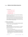
Chapter 3. Wideline Solids Module Operation ............................................. 36
3.1
3.2
3.3
3.4
3.5
3.6
Wideline Solids Module ..............................................................................................
Wideline Experiments .................................................................................................
SSECHO Pulse Sequence ...........................................................................................
Data Acquisition ..........................................................................................................
Standard Wideline Samples ........................................................................................
Data Processing ...........................................................................................................
36
40
41
42
43
45
Chapter 4. CRAMPS/Multipulse Module Operation ..................................... 46
4.1
4.2
4.3
4.4
CRAMPS/Multipulse Module Hardware ....................................................................
Running the FLIPFLIP Pulse Sequence .....................................................................
Running the FLIPFLOP Pulse Sequence ....................................................................
Using MREV8 to Demonstrate Multipulse Operation ................................................
46
48
49
50
Chapter 5. Solid-State NMR Accessories ..................................................... 52
5.1 Pneumatics/Tachometer Box ....................................................................................... 52
5.2 Rotor Synchronization Operation ............................................................................... 52
5.3 Rotor Speed Controller Accessory Operation ............................................................. 56
01-999162-00 A0800
VNMR 6.1C User Guide: Solid-State NMR
4
Table of Contents
5.4 Variable Temperature Operation with Solids .............................................................. 58
Chapter 6. Solid-State NMR Experiments .................................................... 60
6.1 XPOLAR—Cross-Polarization, UNITY .................................................................... 61
6.2 XPOLAR1—Cross-Polarization, UNITYINOVA & UNITYplus .................................... 65
6.3 XPWXCAL—Observe-Pulse Calibration with Cross-Polarization ............................ 67
6.4 XNOESYSYNC—Rotor Sync Solids Sequence for Exchange .................................. 69
6.5 MASEXCH1—Phase-Sensitive Rotor Sync Sequence for Exchange ........................ 70
6.6 HETCORCP1—Solid-State HETCOR ....................................................................... 71
6.7 WISE1—Two-Dimensional Proton Wideline Separation ........................................... 72
6.8 XPOLWFG1—Cross-Polarization with Programmed Decoupling ............................ 73
6.9 XPOLXMOD1—Waveform Modulated Cross-Polarization ...................................... 74
6.10 VACP—Variable Amplitude Cross-Polarization ....................................................... 76
6.11 XPOLEDIT1—Solids Spectral Editing .................................................................... 78
6.12 3QMAS1—Triple-Quantum 2D for Quadrupole Nuclei .......................................... 79
6.13 PASS1—2D Sideband Separation for CP/MAS ....................................................... 80
6.14 CPCS—Cross-Polarization with Proton Chemical Shift Selection .......................... 82
6.15 CPCOSYPS—Cross-Polarization Phase-Sensitive COSY ....................................... 83
6.16 CPNOESYPS—Cross-Polarization Phase-Sensitive NOESY .................................. 84
6.17 R2SELPULS1—Rotation Resonance with Selective Inversion ............................... 86
6.18 DIPSHFT1—Separated Local Field Spectroscopy ................................................... 88
6.19 SEDRA2—Simple Excitation of Dephasing Rotational-Echo Amplitudes .............. 89
6.20 REDOR1—Rotational Echo Double Resonance ...................................................... 91
6.21 DOUBLECP1—Double Cross-Polarization ............................................................. 93
6.22 T1CP1—T1 Measurement with Cross-Polarization .................................................. 95
6.23 HAHNCP1—Spin 1/2 Echo Sequence with CP ....................................................... 95
6.24 SSECHO1—Solid-State Echo Sequence for Wideline Solids .................................. 97
6.25 WLEXCH1—Wideline Solids Exchange ................................................................. 99
6.26 CRAMPS—Combined Rotation and Multiple-Pulse Spectroscopy ....................... 100
6.27 FLIPFLIP—90-Degree Pulse Calibration ............................................................... 103
6.28 FLIPFLOP—Phase Transient Removal .................................................................. 103
6.29 HS90—90-Degree° Phase Shift Accuracy .............................................................. 104
6.30 MREV8, Cycled MREV8—Multiple-Pulse Line Narrowing ................................. 106
6.31 BR24, Cycled BR24—Multiple-Pulse Line Narrowing ......................................... 107
6.32 CORY24, Cycled CORY24—Multiple-Pulse Line Narrowing .............................. 108
6.33 MREVCS—Multiple Pulse Chemical-Shift Selective Spin Diffusion ................... 109
6.34 MQ_SOLIDS—Multiple-Quantum Solids ............................................................. 110
6.35 SPINDIFF—Spin Diffusion in Solids .................................................................... 111
6.36 FASTACQ—Multinuclear Fast Acquisition ........................................................... 112
6.37 NUTATE—Solids 2D Nutation .............................................................................. 113
Index ............................................................................................................... 116
5
VNMR 6.1C User Guide: Solid-State NMR
01-999162-00 A0800
List of Figures
Figure 1. Linear Attenuator Control Graph ..................................................................................
Figure 2. Typical MAS Spectrum of Adamantane .......................................................................
Figure 3. Tools for Coarse Adjustment of Sample Angle ............................................................
Figure 4. FID Display of KBr on Angle ......................................................................................
Figure 5. FID Display of KBr 1/2 Turn Off Angle ......................................................................
Figure 6. Typical Hexamethylbenzene (HMB) Spectrum ............................................................
Figure 7. Array of Contact Times ................................................................................................
Figure 8. TOSS Experiment on Alanine (Spectrum and Sequence) ............................................
Figure 9. Protonated Carbon Suppression of Alanine (Spectrum and Sequence) ........................
Figure 10. Rotating-Frame Spin-Lattice Relaxation Measurements Sequence ...........................
Figure 11. Pulse Sequence for Measuring lH T1 ..........................................................................
Figure 12. Solids Cabinet Layout, Open Front View ...................................................................
Figure 13. High-Power Amplifiers Status Panel ..........................................................................
Figure 14. Real Channel FID Pattern ...........................................................................................
Figure 15. FLIPFLIP FID at Exact 90° Pulse ..............................................................................
Figure 16. FLIPFLOP “Tram Tracks” .........................................................................................
Figure 17. FLIPFLOP Desired FID .............................................................................................
Figure 18. Pneumatics/Tachometer Box for CP/MAS Probes ....................................................
Figure 19. Different Modes of the Rotor Synchronization Accessory .........................................
Figure 20. Base of a Varian High-Speed Spinning Rotor ............................................................
Figure 21. Doty Double Bearing Rotor .......................................................................................
Figure 22. TOSS Pulse Sequence ................................................................................................
Figure 23. Protonated Carbon Suppression Sequence .................................................................
Figure 24. Rotating-Frame Spin-Lattice Relaxation Measurements Sequence ...........................
Figure 25. Pulse Sequence for Measuring lH T1 ..........................................................................
Figure 26. XPOLAR1 Pulse Sequence ........................................................................................
Figure 27. XPWXCAL Pulse Sequence ......................................................................................
Figure 28. XNOESYSYNC Pulse Sequence ...............................................................................
Figure 29. MASEXCH1 Pulse Sequence ....................................................................................
Figure 30. XPOLXMOD1 Pulse Sequence .................................................................................
Figure 31. VACP Pulse Sequence ................................................................................................
Figure 32. XPOLDIT1 Pulse Sequence .......................................................................................
Figure 33. 3QMAS1 Pulse Sequence ..........................................................................................
Figure 34. PASS1 Pulse Sequence ...............................................................................................
Figure 35. CPCS Pulse Sequence ................................................................................................
Figure 36. CPCOSYPS Pulse Sequence ......................................................................................
Figure 37. CPNOESYPS Pulse Sequence ...................................................................................
Figure 38. R2SELPULS1 Pulse Sequence ..................................................................................
Figure 39. DIPSHFT1 Pulse Sequence ........................................................................................
Figure 40. SEDRA2 Pulse Sequence ...........................................................................................
01-999162-00 A0800
VNMR 6.1C User Guide: Solid-State NMR
19
25
25
26
27
27
30
31
32
33
33
38
40
48
49
50
50
53
53
54
54
62
63
63
64
66
68
69
70
75
77
78
79
81
82
83
85
86
88
90
6
List of Figures
Figure 41. REDOR1 Pulse Sequence .......................................................................................... 91
Figure 42. DOUBLECP1 Pulse Sequence ................................................................................... 94
Figure 43. T1CP1 Pulse Sequence ............................................................................................... 95
Figure 44. HAHNCP1 Pulse Sequence ........................................................................................ 96
Figure 45. SSECHO1 Pulse Sequence ......................................................................................... 98
Figure 46. WLEXCH1 Pulse Sequence ..................................................................................... 100
Figure 47. FLIPFLOP Pulse Sequence ...................................................................................... 104
Figure 48. HS90 Pulse Sequence ............................................................................................... 105
Figure 49. MREV8 Pulse Sequence .......................................................................................... 106
Figure 50. BR24 Pulse Sequence ............................................................................................... 107
Figure 51. Cycled CORY24 Pulse Sequence ............................................................................. 108
Figure 52. CORY24 Pulse Sequence ......................................................................................... 108
Figure 53. MREVCS Pulse Sequence ........................................................................................ 110
Figure 54. MQ_SOLIDS Pulse Sequence .................................................................................. 111
Figure 55. SPINDIFF Pulse Sequence ....................................................................................... 111
Figure 56. FASTACQ Pulse Sequence ....................................................................................... 113
Figure 57. NUTATE Pulse Sequence ......................................................................................... 113
List of Tables
Table 1. Background Nuclei of Rotor Material ............................................................................. 20
Table 2. Typical Spin Rates with Associated Bearing and Drive Values ....................................... 22
Table 3. Reference Materials and 13C Chemical Shifts ................................................................. 34
Table 4. Bessel Filter Outputs ........................................................................................................ 37
Table 5. Wideline Experiment Commands and Parameters ........................................................... 41
Table 6. Rotor Synchronization Controls ...................................................................................... 55
Table 7. Rotor Controller Gain Setting and Typical Ranges ......................................................... 57
Table 8. Multiacquisition Quadrature Corrections for MREV8 .................................................. 102
Table 9. Multiacquisition Quadrature Corrections for BR24 ...................................................... 102
Table 10. Multiacquisition Quadrature Corrections for CORY24 ............................................... 102
7
VNMR 6.1C User Guide: Solid-State NMR
01-999162-00 A0800
SAFETY PRECAUTIONS
The following warning and caution notices illustrate the style used in Varian manuals
for safety precaution notices and explain when each type is used:
WARNING: Warnings are used when failure to observe instructions or precautions
could result in injury or death to humans or animals, or significant
property damage.
CAUTION:
Cautions are used when failure to observe instructions could result in
serious damage to equipment or loss of data.
Warning Notices
Observe the following precautions during installation, operation, maintenance, and
repair of the instrument. Failure to comply with these warnings, or with specific
warnings elsewhere in Varian manuals, violates safety standards of design,
manufacture, and intended use of the instrument. Varian assumes no liability for
customer failure to comply with these precautions.
WARNING: Persons with implanted or attached medical devices such as
pacemakers and prosthetic parts must remain outside the 5-gauss
perimeter of the magnet.
The superconducting magnet system generates strong magnetic fields that can
affect operation of some cardiac pacemakers or harm implanted or attached
devices such as prosthetic parts and metal blood vessel clips and clamps.
Pacemaker wearers should consult the user manual provided by the pacemaker
manufacturer or contact the pacemaker manufacturer to determine the effect on
a specific pacemaker. Pacemaker wearers should also always notify their
physician and discuss the health risks of being in proximity to magnetic fields.
Wearers of metal prosthetics and implants should contact their physician to
determine if a danger exists.
Refer to the manuals supplied with the magnet for the size of a typical 5-gauss
stray field. This gauss level should be checked after the magnet is installed.
WARNING: Keep metal objects outside the 10-gauss perimeter of the magnet.
The strong magnetic field surrounding the magnet attracts objects containing
steel, iron, or other ferromagnetic materials, which includes most ordinary
tools, electronic equipment, compressed gas cylinders, steel chairs, and steel
carts. Unless restrained, such objects can suddenly fly towards the magnet,
causing possible personal injury and extensive damage to the probe, dewar, and
superconducting solenoid. The greater the mass of the object, the more the
magnet attracts the object.
Only nonferromagnetic materials—plastics, aluminum, wood, nonmagnetic
stainless steel, etc.—should be used in the area around the magnet. If an object
is stuck to the magnet surface and cannot easily be removed by hand, contact
Varian service for assistance.
01-999162-00 A0800
VNMR 6.1C User Guide: Solid-State NMR
8
SAFETY PRECAUTIONS
Warning Notices (continued)
Refer to the manuals supplied with the magnet for the size of a typical 10-gauss
stray field. This gauss level should be checked after the magnet is installed.
WARNING: Only qualified maintenance personnel shall remove equipment covers
or make internal adjustments.
Dangerous high voltages that can kill or injure exist inside the instrument.
Before working inside a cabinet, turn off the main system power switch located
on the back of the console.
WARNING: Do not substitute parts or modify the instrument.
Any unauthorized modification could injure personnel or damage equipment
and potentially terminate the warranty agreements and/or service contract.
Written authorization approved by a Varian, Inc. product manager is required
to implement any changes to the hardware of a Varian NMR spectrometer.
Maintain safety features by referring system service to a Varian service office.
WARNING: Do not operate in the presence of flammable gases or fumes.
Operation with flammable gases or fumes present creates the risk of injury or
death from toxic fumes, explosion, or fire.
WARNING: Leave area immediately in the event of a magnet quench.
If the magnet dewar should quench (sudden appearance of gasses from the top
of the dewar), leave the area immediately. Sudden release of helium or nitrogen
gases can rapidly displace oxygen in an enclosed space creating a possibility of
asphyxiation. Do not return until the oxygen level returns to normal.
WARNING: Avoid helium or nitrogen contact with any part of the body.
In contact with the body, helium and nitrogen can cause an injury similar to a
burn. Never place your head over the helium and nitrogen exit tubes on top of
the magnet. If helium or nitrogen contacts the body, seek immediate medical
attention, especially if the skin is blistered or the eyes are affected.
WARNING: Do not look down the upper barrel.
Unless the probe is removed from the magnet, never look down the upper
barrel. You could be injured by the sample tube as it ejects pneumatically from
the probe.
WARNING: Do not exceed the boiling or freezing point of a sample during variable
temperature experiments.
A sample tube subjected to a change in temperature can build up excessive
pressure, which can break the sample tube glass and cause injury by flying glass
and toxic materials. To avoid this hazard, establish the freezing and boiling
point of a sample before doing a variable temperature experiment.
9
VNMR 6.1C User Guide: Solid-State NMR
01-999162-00 A0800
SAFETY PRECAUTIONS
Warning Notices (continued)
WARNING: Support the magnet and prevent it from tipping over.
The magnet dewar has a high center of gravity and could tip over in an
earthquake or after being struck by a large object, injuring personnel and
causing sudden, dangerous release of nitrogen and helium gasses from the
dewar. Therefore, the magnet must be supported by at least one of two methods:
with ropes suspended from the ceiling or with the antivibration legs bolted to
the floor. Refer to the Installation Planning Manual for details.
WARNING: Do not remove the relief valves on the vent tubes.
The relief valves prevent air from entering the nitrogen and helium vent tubes.
Air that enters the magnet contains moisture that can freeze, causing blockage
of the vent tubes and possibly extensive damage to the magnet. It could also
cause a sudden dangerous release of nitrogen and helium gases from the dewar.
Except when transferring nitrogen or helium, be certain that the relief valves are
secured on the vent tubes.
WARNING: On magnets with removable quench tubes, keep the tubes in place
except during helium servicing.
On Varian 200- and 300-MHz 54-mm magnets only, the dewar includes
removable helium vent tubes. If the magnet dewar should quench (sudden
appearance of gases from the top of the dewar) and the vent tubes are not in
place, the helium gas would be partially vented sideways, possibly injuring the
skin and eyes of personnel beside the magnet. During helium servicing, when
the tubes must be removed, follow carefully the instructions and safety
precautions given in the magnet manual.
Caution Notices
Observe the following precautions during installation, operation, maintenance, and
repair of the instrument. Failure to comply with these cautions, or with specific
cautions elsewhere in Varian manuals, violates safety standards of design,
manufacture, and intended use of the instrument. Varian assumes no liability for
customer failure to comply with these precautions.
CAUTION:
Keep magnetic media, ATM and credit cards, and watches outside the
5-gauss perimeter of the magnet.
The strong magnetic field surrounding a superconducting magnet can erase
magnetic media such as floppy disks and tapes. The field can also damage the
strip of magnetic media found on credit cards, automatic teller machine (ATM)
cards, and similar plastic cards. Many wrist and pocket watches are also
susceptible to damage from intense magnetism.
Refer to the manuals supplied with the magnet for the size of a typical 5-gauss
stray field. This gauss level should be checked after the magnet is installed.
01-999162-00 A0800
VNMR 6.1C User Guide: Solid-State NMR
10
SAFETY PRECAUTIONS
Caution Notices (continued)
CAUTION:
Check helium and nitrogen gas flowmeters daily.
Record the readings to establish the operating level. The readings will vary
somewhat because of changes in barometric pressure from weather fronts. If
the readings for either gas should change abruptly, contact qualified
maintenance personnel. Failure to correct the cause of abnormal readings could
result in extensive equipment damage.
CAUTION:
Never operate solids high-power amplifiers with liquids probes.
On systems with solids high-power amplifiers, never operate the amplifiers
with a liquids probe. The high power available from these amplifiers will
destroy liquids probes. Use the appropriate high-power probe with the highpower amplifier.
CAUTION:
Take electrostatic discharge (ESD) precautions to avoid damage to
sensitive electronic components.
Wear grounded antistatic wristband or equivalent before touching any parts
inside the doors and covers of the spectrometer system. Also, take ESD
precautions when working near the exposed cable connectors on the back of the
console.
Radio-Frequency Emission Regulations
The covers on the instrument form a barrier to radio-frequency (rf) energy. Removing
any of the covers or modifying the instrument may lead to increased susceptibility to
rf interference within the instrument and may increase the rf energy transmitted by the
instrument in violation of regulations covering rf emissions. It is the operator’s
responsibility to maintain the instrument in a condition that does not violate rf emission
requirements.
11
VNMR 6.1C User Guide: Solid-State NMR
01-999162-00 A0800
Introduction
This manual is designed to help you perform solid-state NMR experiments using a Varian
solid-state NMR module on a Varian NMR spectrometer system running VNMR version
6.1C software. The manual contains the following chapters:
• Chapter 1, “Overview of Solid-State NMR,” provides an short overview of solid-state
NMR, including the types of solids modules, probes, and accessories available.
• Chapter 2, “CP/MAS Solids Operation,” covers using the CP/MAS solids module.
• Chapter 3, “Wideline Solids Module Operation,” covers using the wideline solids
module.
• Chapter 4, “CRAMPS/Multipulse Module Operation,” covers using the CPAMPS/
multipulse module.
• Chapter 5, “Solid-State NMR Accessories,” covers using the rotor synchronization,
rotor speed controller accessory, and solids variable temperature accessories.
• Chapter 6, “Solid-State NMR Experiments,” is a guide to more than 40 pulse
sequences useful for performing solid-state NMR experiments.
Notational Conventions
The following notational conventions are used throughout all VNMR manuals:
• Typewriter-like characters identify VNMR and UNIX commands, parameters,
directories, and file names in the text of the manual. For example:
The shutdown command is in the /etc directory.
• The same type of characters show text displayed on the screen, including the text
echoed on the screen as you enter commands during a procedure. For example:
Self test completed successfully.
• Text shown between angled brackets in a syntax entry is optional. For example, if the
syntax is seqgen s2pul<.c>, entering the “.c” suffix is optional, and typing
seqgen s2pul.c or seqgen s2pul is functionally the same.
• Lines of text containing command syntax, examples of statements, source code, and
similar material are often too long to fit the width of the page. To show that a line of
text had to be broken to fit into the manual, the line is cut at a convenient point (such
as at a comma near the right edge of the column), a backslash (\) is inserted at the cut,
and the line is continued as the next line of text. This notation will be familiar to C
programmers. Note that the backslash is not part of the line and, except for C source
code, should not be typed when entering the line.
• Because pressing the Return key is required at the end of almost every command or
line of text you type on the keyboard, use of the Return key will be mentioned only in
cases where it is not used. This convention avoids repeating the instruction “press the
Return key” throughout most of this manual.
• Text with a change bar (like this paragraph) identifies material new to VNMR 6.1C that
was not in the previous version of VNMR. Refer to the document Release Notes for a
description of new features to the software.
01-999162-00 A0800
VNMR 6.1C User Guide: Solid-State NMR
12
Introduction
Other Manuals
This manual should be your basic source for information about using the spectrometer
hardware and software on a day-to-day basis for solid-state NMR. Other VNMR manuals
you should have include:
• Getting Started
• Walkup NMR Using GLIDE
• User Guide: Liquids NMR
• VNMR Command and Parameter Reference
• VNMR User Programming
• VNMR and Solaris Software Installation
All of these manuals are shipped with the VNMR software. These manuals, other Varian
hardware and installation manuals, and most Varian accessory manuals are also provided
online so that you can view the pages on your workstation and print copies.
Types of Varian NMR Spectrometer Systems
In parts of this manual, the type of spectrometer system (UNITYINOVA, MERCURY-VX,
MERCURY, GEMINI 2000, UNITYplus, UNITY, or VXR-S) must be considered in order to
use the software properly.
•
UNITY
INOVA and MERCURY-VX are the current systems sold by Varian.
• UNITYplus, UNITY, and VXR-S are spectrometer lines that preceded the UNITYINOVA.
• MERCURY and GEMINI 2000 are spectrometer lines that preceded the MERCURY-VX.
Help Us to Meet Your Needs!
We want to provide the equipment, publications, and help that you want and need. To do
this, your feedback is most important. If you have ideas for improvements or discover a
problem in the software or manuals, we encourage you to contact us. You can reach us at
the nearest Varian Applications Laboratory or at the following address:
Palo Alto Applications Laboratory
Varian, Inc., NMR Systems
3120 Hansen Way, MS D-298
Palo Alto, California 94304 USA
13
VNMR 6.1C User Guide: Solid-State NMR
01-999162-00 A0800
Chapter 1.
Overview of Solid-State NMR
Sections in this chapter:
• 1.1 “Line Broadening,” this page
• 1.2 “Spin-Lattice Relaxation Time,” page 15
• 1.3 “Solids Modules, Probes, and Accessories,” page 15
Before techniques were developed to obtain high-resolution NMR spectra of compounds in
the solid state, the spectra of these samples were generally characterized by broad,
featureless envelopes caused by additional nuclear interactions present in solid state. In
liquid state, these interactions average to zero due to rapid molecular tumbling.
1.1 Line Broadening
One cause of line broadening is heteronuclear and homonuclear dipolar coupling. This
coupling arises from the interaction of the nuclear magnetic dipole under observation with
those of the surrounding nuclei, and is directly proportional to the magnetogyric ratios of
the nuclei and inversely proportional to the distance between them. In strongly coupled
organic solids, the heteronuclear dipolar coupling between a 13C nucleus and a bonded
proton can be 40 kHz. In order to remove the heteronuclear dipolar coupling, a strong rf
field equal to or greater than the interaction energy must be applied at the proton resonance
frequency.
A second cause of line broadening in polycrystalline compounds is chemical shift
anisotropy (CSA). This is the result of nuclei with different orientations in the applied
magnetic field resonating at different Larmor frequencies. The observed spread of the
chemical shifts is called the chemical shift anisotropy and can be as large as a few hundred
ppm. This interaction can be removed by rapidly rotating the sample about an axis oriented
at an angle of 54 degrees 44 minutes (54.73°, the “magic angle” in magic angle spinning,
or MAS to the applied magnetic field. The spinning speed of the sample must be greater
than the CSA in order to reduce the resonance to a single, narrow (approximately 1 ppm)
line at the isotropic frequency. If the spinning speed is less than the CSA, a pattern of
sidebands occurs about the isotropic peak at integral values of the spinning frequency. The
CSA scales linearly with B0.
A third source of line broadening in solids occurs when observing nuclei that possess an
electric quadrupole. The quadrupolar interaction can be as large as several MHz. For
nonintegral spin quadrupolar nuclei, the central transition is much narrower (about 10 kHz)
and therefore can be narrowed to a single, narrow line by magic angle spinning. The
residual (second order) linewidth of the central transition is inversely proportional to the
applied magnetic field.
01-999162-00 A0800
VNMR 6.1C User Guide: Solid-State NMR
14
Chapter 1. Overview of Solid-State NMR
1.2 Spin-Lattice Relaxation Time
An additional characteristic of some nuclei in the solid state, for example 13C, is a long
spin-lattice relaxation time (T1). To overcome this problem, the abundant nuclei (usually
protons) in the system are used. These are polarized with a spin locking pulse (CP). The
polarization is then transferred to the rare spins by applying an rf field at the Larmor
frequency of the rare spins that is of such a magnitude as to make the energy levels of the
abundant and rare spins the same in the rotating frame (Hartmann-Hahn match condition).
Following a transfer of energy from the polarized abundant spins to the rare spins, the rare
spin field is turned off and the resulting signal observed under conditions of high-power
proton decoupling. The recycle time is then set according to the proton T1, which is usually
much shorter than the rare spin T1.
The polarization transfer can give an increase in sensitivity. The rare spin response is
enhanced by a factor of up to the ratio of the magnetogyric ratios of the two spin systems.
For the 13C-{1H} system, this is a factor of 4. However, as the enhancement is distance
related, caution should be exercised in using the cross-polarization experiment for
quantitative analysis.
1.3 Solids Modules, Probes, and Accessories
Varian supplies a complete line of solid-state NMR modules, probes, and accessories.
Solids modules include CP/MAS, wideline, CRAMPS/multipulse, and complete solids.
CP/MAS, wideline, and CRAMPS/Multipulse hardware and operation are covered in
Chapters 2, 3, and 4, respectively, of this manual.
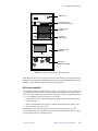
The Varian complete solids module is capable of performing all experiments possible with
the Varian CP/MAS, wideline, and CRAMPS/multipulse modules. The major components
of complete solids module are the following:
UNITY
INOVA or UNITYplus System
UNITY or VXR-S System
Wideband ADC with Sum to Memory
Solids cabinet
High-band & low-band 1-kW amplifier
Pneumatics/tachometer box
Wideband ADC
Solids cabinet
High-band & low-band 1-kW amplifier
Pneumatics/tachometer box
Wideband receiver
Sync module
Two fine attenuators
For operation of the complete solids module, refer to the operations sections in the chapters
2 to 4 for the CP/MAS, wideline, and CRAMPS/multipulse modules.
A wide variety of solids probes and probe accessories are available, including wideline,
multipulse, and magic-angle probes.
Optional solids accessories include rotor synchronization, rotor speed controller, and the
solids variable temperature accessory. Chapter 5 covers using these accessories.
15
VNMR 6.1C User Guide: Solid-State NMR
01-999162-00 A0800
Chapter 2.
CP/MAS Solids Operation
Sections in this chapter:
• 2.1 “CP/MAS Solids Modules,” this page.
• 2.2 “Preparing the Sample and Rotor,” page 18.
• 2.3 “Spinning the Sample,” page 20.
• 2.4 “Adjusting Homogeneity,” page 22.
• 2.5 “Adjusting the Magic Angle,” page 22.
• 2.6 “XPOLAR Pulse Sequence,” page 26.
• 2.7 “Calibrating Pulse Width,” page 26.
• 2.8 “Calibrating Decoupler Power,” page 26.
• 2.9 “Adjusting the Hartmann-Hahn Match,” page 27.
• 2.10 “Optimizing Parameters and Special Experiments,” page 27.
• 2.11 “Spectral Referencing,” page 31.
• 2.12 “Further Reading on Solid-State NMR,” page 32.
• 2.13 “Useful Conversions,” page 33.
2.1 CP/MAS Solids Modules
CP/MAS hardware differs between systems.
CP/MAS Hardware for UNITYINOVA and UNITYplus systems
On UNITYINOVA and UNITYplus systems, CP/MAS hardware consists of a class A/B AMT
3900A-15 linear amplifier that replaces the standard liquids linear amplifier. The CP/MAS
linear amplifier produces output power of up to 100 W in the high band (1H/19F) for up to
250 ms. The low band remains the same as for the original standard liquids amplifier.
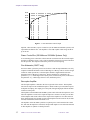
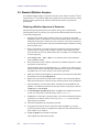
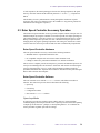
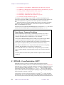
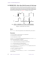
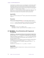
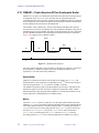
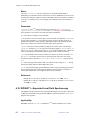
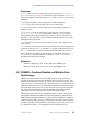
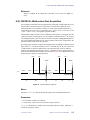
The fine power control over a range of 0 to 60 dB in 4095 steps is provided by the
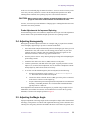
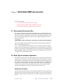
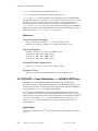
Transmitter board, which is standard on UNITYINOVA and UNITYplus systems. The
parameters controlling this are dpwrm, dpwrm2, and dpwrm3. The attenuator control is
linear, meaning the control is finer in the higher region than in the lower region of the
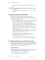
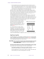
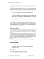
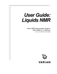
attenuator, as shown in Figure 1. In addition, a pneumatics/tachometer box is used for
controlling air flow and spinning speeds.
CP/MAS Hardware for UNITY and VXR-S Systems
The CP/MAS solids module is the only one of the solids hardware configurations that does
not require the solids cabinet. Apart from the special probe, the hardware for the standardperformance CP/MAS solids module consists of a 100 W, narrow-band decoupler pulse
01-999162-00 A0800
VNMR 6.1C User Guide: Solid-State NMR
16
Chapter 2. CP/MAS Solids Operation
60 dB
54 dB
48 dB
42 dB
36 dB
0 dB
0 255 511
1023
2047
4095
Figure 1. Linear Attenuator Control Graph
amplifier, a fine attenuator, a power control box (on 200 MHz and 300 MHz systems), and
a pneumatics/tachometer box. The amplifier is class AB, capable of delivering 100 W for
up to 250 ms.
Power Control Box (200-MHz and 300-MHz Systems Only)
A free-standing power control box with an ON/OFF switch activates the 100 W decoupler
and observe amplifiers (class C only). This box should be located in a convenient location
near the operator. The computer controls the power levels for decoupling.
Fine Attenuator (UNITY only)
In a basic UNITY system, the power levels for observe and decouple transmitters are set by
computer-controlled attenuators with a 63-dB range in 1-dB steps. This is not fine enough
control for solids experiments, so the decoupler channel is supplemented with a fine
attenuator with a 6-dB range in 4096 steps. The fine attenuator is controlled by the
parameter dpwrf, which ranges from 0 (least power) to 4095 (most power). VXR-S uses
the parameter dhp, which ranges from 0 to 255 (maximum power).
Decoupler Amplifier
The decoupler amplifier is housed in the lower right side of the console. This amplifier
increases the output of the standard decoupler to about 100 W to provide sufficient power
for dipolar decoupling. The output goes to the probe, through a high-pass filter at the DEC
connector on the probe.
The amplifier on the 200 MHz and 300 MHz systems can be left in the decoupler line, since
when the amplifier is turned off, its input and output are connected. A safety circuit shuts
off the amplifier and sounds a buzzer if the output of the amplifier is not connected to 50
ohms. If this happens, the ON/OFF switch on the amplifier must be turned to off, the fault
rectified, and then the switch turned back to on.
The amplifier on the 400 MHz system has a separate power switch instead of the control
box, and when the amplifier is turned off, the input and output are not connected. Included
on this amplifier is dynamic overload protection.
17
VNMR 6.1C User Guide: Solid-State NMR
01-999162-00 A0800
2.2 Preparing the Sample and Rotor
The decouple amplifier is driven by the normal liquids decoupler output, which can be as
high as 50 W at maximum output. This is more than sufficient to drive the decoupler
amplifier, and if used at full power, can damage the decoupler. Although the parameter
level2 has been set to 63 in this manual, do not use values higher than those that deliver
25 W (200- and 300-MHz systems) or 10 W (400-MHz system) to the input of the
decoupler amplifier.
2.2 Preparing the Sample and Rotor
Solid samples are normally packed into hollow rotors. These rotors are sealed with fluted
caps that are driven for spinning. The method of filling the rotors depends somewhat on the
form and nature of the sample. The most critical factor in spinning reliability is the dynamic
balance of the filled rotor. Some specific recommendations on filling the rotors and
achieving a reasonable balance for different kinds of samples are given below.
Rotor Composition
Doty rotors are either of zirconia, silicon nitride, or sapphire, with Kel-F or Vespel end caps.
See the manual from the rotor manufacturer for details.
Varian high-speed rotors are composed of zirconia or of silicon nitride (Si3N4) with pMMA
or Torlon (type 4203) end caps. Refer to the probe installation manual for a list of rotors
and end caps and their associated part numbers, color, temperature range, and maximum
spin rates.
During VT operation, Torlon end caps can exceed the +100°C specification of the 7-mm
probe. Below -100°C, a potential for slipping due to differential contraction with the
ceramic rotor exists. Kel-F end caps (colorless-opaque) have a VT upper limit of about
+70°C and should not be spun faster than 6500 Hz at any temperature. pMMA end caps
(colorless-clear) must only be used at room temperature and below. These are currently
supplied with Varian RT CP/MAS probes. Visually distinguishing between Kel-F and
pMMA end caps can be difficult, so you may want to mark them appropriately. The
background nuclei for these materials are listed in Table 1.
Table 1. Background Nuclei of Rotor Material
CAUTION:
Material
Background
Kel-F end cap
C (not cross-polarizable), F
Vespel, Torlon, pMMA end cap
C (cross-polarizable), H
sapphire rotor
Al, O
zirconia rotor
Zr, O, traces of Mg, Y, Al
Si3N4 rotor
Si, N, some Al
Spinning a rotor for more than a few minutes in a vibrating state can
cause permanent damage to the bearing surface of both the rotor and
stator. Once this happens the rotor will probably not spin adequately
again, even if perfectly balanced.
01-999162-00 A0800
VNMR 6.1C User Guide: Solid-State NMR
18
Chapter 2. CP/MAS Solids Operation
Homogeneous Machinable Solids
Although some hard machinable polymers can be made directly into solid rotors, it is much
easier to make a plug for the standard hollow rotor. The signal-to-noise difference is not that
significant. The fit must be tight enough to prevent the plug from rattling around or slipping
out during spinning. The sample material must be homogeneous and free of voids for the
spinning rotor to remain balanced.
One way to remove a sample plug is to drill and tap a center hole about halfway through
the plug for a 2-56 screw. This is best done on a lathe to facilitate centering and ensure
balance. A small screw is then used to extract the plug.
For Varian 7-mm rotors, the solid sample should be machined as a plug to fit into the rotor.
Ideal dimensions should be 0.440 ± 0.005 in. (11.176 mm) long, by 0.1960 ± 0.0005 in.
(4.979 mm) in diameter (0.137 in. (3.48 mm) for Varian 5-mm rotors).
Granular and Powdered Materials
For granular or powder materials, the best method for filling the rotors is by pouring the
material into the rotor, leaving just enough room for the cap. Granular and powdered
materials work best as uniform fine particles (100 mesh or finer). If the material can be
ground, it is better to do so before attempting to pack the rotor (a mortar and pestle is
usually sufficient). Fluffy or flaky materials can be packed with a rod machined to a slightly
smaller diameter than the internal diameter (ID) of the rotor. Hand pressure should be
sufficient. Hard packing with a press or hammer is not necessary and can damage the rotors.
The cap works best if it is in contact with the top of the sample material and fits snugly and
flush with the top of the rotor.
Miscellaneous Materials
Many different sample types and forms exist that are neither machinable solids nor granular
or powdered materials. Some of these materials can be prepared in rotors so that dynamic
balance is preserved, while others cannot. Basically, if the material can be made to fill the
rotor homogeneously, chances are good that it will spin adequately.
Thick sheet or film materials are best handled by cutting or punching many disks, each
having the inside diameter of the rotor, and stacking them in the rotor until full.
Coarse and irregular granular materials as well as pellets, beads, flakes, bits, or pieces often
cannot be packed homogeneously enough to provide the balance necessary for high speed
spinning. Sometimes such materials can be made to spin smoothly by filling the voids with
a fine powder that does not give NMR signals, such as KBr, talc, or sulfur flowers and
spinning at a lower speed.
CAUTION:
Organic solvents can dissolve pMMA end caps.
Liquid Samples
For liquid samples, use an end cap that has a concentric hole drilled through it (a #73 drill
is recommended). Be sure the end cap will not dissolve (organic solvents can dissolve
pMMA end caps). Liquid samples can be spun at several hundred Hz, but the liquid may
spin out of the rotor and be lost. This fact must be considered when dealing with toxic or
noxious samples.
19
VNMR 6.1C User Guide: Solid-State NMR
01-999162-00 A0800
2.3 Spinning the Sample
2.3 Spinning the Sample
On Varian high-speed rotors, tachometer sensing is on the rotor bottom. Zirconia rotors are
marked with a permanent black marking pen or black enamel so that 50% of the bottom of
surface area is shaded black; silicon nitride (Si3N4) rotors are marked with white enamel in
the same fashion.
Centrifugal force can cause the black and white markings to flake off around the edges. This
can cause inaccurate tachometer readings. The black or white half circle can be reapplied
on the rotors with a black marking pen and white correction fluid. The diameter marking
should be straight.
Doty high-speed rotors have optical markings inside the bottom cap; other Doty probes use
electrostatic sensing (triboelectric). See the Doty manual for instructions on reapplying the
optical marking.
WARNING: A projectile hazard exists if a spinning rotor explodes. To prevent
possible eye injury from an exploding rotor, avoid spinning rotors
outside the magnet. If it is necessary to spin a rotor outside the
magnet, use a certified safety shield and full face shield at all times.
Never use rotors that have been dropped onto a hard surface, since
microscopic cracks in the rotor material can cause rotor explosions at
much lower spinning speeds than indicated in Table 2. Never spin
zirconia (white) rotors at spinning speeds above 7.2 kHz. Never spin
silicon nitride (gray) rotors at speeds above 9.5 kHz. Never apply air
drive pressure above 72.5 psig (5.0 bar).
Table 2. Typical Spin Rates with Associated Bearing and Drive Values
Bearing
Spinning Speed
(Hz ±250 Hz)
Drive
Pressure
psig (bar)
Flow rate
(LPM ±2 LPM)
Pressure
psig (bar)
Flow rate
(LPM ±2 LPM)
2500
28 (2.0)
12.5
7 (0.5)
15.0
4000
28 (2.0)
12.5
14 (1.0)
20.0
5000
36 (2.5)
12.5
21 (1.5)
25.0
6000
36 (2.5)
12.5
28 (2.0)
27.5
6500
36 (2.5)
12.5
35 (2.4)
29.5
7200
36 (2.5)
12.5
36 (2.5)
30.0
7500
39 (2.7)
12.5
44 (3.0)
32.5
8000
44 (3.0)
10.0
51 (3.5)
35.0
8500
44 (3.0)
10.0
58 (4.0)
37.5
9000
44 (3.0)
09.0
65 (4.5)
40.0
To Spin Samples in Doty Probes
Either one or two air supplies can be used for sample spinning in the Doty probe. Because
the control box supplied for CP/MAS has two controllers, split streams are recommended.
The techniques for doing this are covered in the Doty probe manual.
01-999162-00 A0800
VNMR 6.1C User Guide: Solid-State NMR
20
Chapter 2. CP/MAS Solids Operation
To Spin Samples in High-Speed Probes
Table 2 lists spin rates and the appropriate bearing and drive pressures for the Varian 7-mm
VT CP/MAS probe at ambient temperature. The spin rates shown are approximate values.
The actual spin rate varies depending on the properties of the sample and sample holder.
Use the following procedure for spinning all samples in high-speed probes:
1.
Using your fingers, insert either an end-cap into the rotor to be spun. Rotate the end
cap while pushing it into the rotor. Make sure the end cap is fully seated into the
rotor.
2.
Make sure the bearing and drive air pressure are off.
3.
Carefully place the rotor with the end cap into the stator and install the probe into
the magnet. Turn the air bearing pressure to 28 psig (2.0 bar); the rotor should start
spinning slowly at 500–900 Hz.
4.
Slowly turn on the air drive pressure to 3.6 psig (0.25 bar) and wait for 15 seconds
to allow the rotor to stabilize.
5.
Gradually increase the air drive pressure to 7 psig (0.5 bar) and again wait 15
seconds. The spinning speed should gradually increase to about 2500 Hz.
6.
Slowly increase the air drive pressure to 14 psig (1.0 bar). The spinning speed should
reach about 3700 Hz.
7.
If rotor speeds faster than 3700 Hz are required, slowly increase the air bearing
pressure to 36 psig (2.5 bar). Then increase the air drive pressure up to 34 psig (2.4
bar); the rotor speed should reach about 7200 Hz. Never apply air drive pressure
above 72.5 psig (5.0 bar).
To avoid rotor explosions, never spin zirconia rotors faster than 7200 Hz or spin silicon
nitride rotors faster than 9500 Hz. For samples that have densities above 3.0 g/cc, decrease
the maximum spin rate by 35%.
It may be necessary to increase the bearing pressure for ill-behaved samples or for very high
spinning speeds. Provided that the two flowmeter valves are fully open, they require no
adjustment at any time. Never adjust the spin rate with the flowmeter.
CAUTION:
To prevent damage to the rotor or bearing, always smoothly shut off
the rotation gas using the rotation pressure regulator before turning
off the bearing gas using the bearing pressure regulator.
To remove a sample, take care to decrease the rotor speed smoothly. At all times that
rotation air is flowing, bearing air should read at least 28 psig (1.9 bar). Only when the
rotation air is completely off should the bearing be carefully decreased to zero.
Overcoming Imbalance
Most of the spinning problems encountered with filled rotors result from imbalance caused
by the sample material. A damaged rotor might be at fault but that can be eliminated by
always checking the spinning quality of the empty rotor before packing it with the sample
material. Discard damaged rotors.
If a packed rotor does not spin properly at first, inspect it to see if the sample has been
disturbed. Part of the sample may have broken loose and been thrown out of the rotor, in
which case, repacking might be the solution. Sometimes loose material balances itself if
kept in the rotor and spun below its vibration speed for a few minutes. If the sample seems
intact on the surface, then it is more than likely not homogeneous or did not pack evenly.
21
VNMR 6.1C User Guide: Solid-State NMR
01-999162-00 A0800
2.4 Adjusting Homogeneity
In the case of a machined plug, the material can have a void or it can fit too loosely in the
rotor cavity. The only solution is to remove all the sample and repack the rotor. With
inhomogeneous materials, this repacking may have to be tried more than once.
CAUTION:
When removing caps or digging out packed samples, take care not to
gouge the rotor. Even small scratches can imbalance the rotor.
At times, worn rotor caps cause imbalance. Changing caps or rotating them between rotors
sometimes cures these problems.
Probe Adjustments for Improved Spinning
Increased bearing pressure often stabilizes samples that do not spin well. This adjustment
must be made at low speed and then ramped up once the rotor spinning is stable.
2.4 Adjusting Homogeneity
Homogeneity should be adjusted as follows on a sample of D2O, prepared in a standard
rotor, and tightly capped using a cap with a concentric drilled hole.
1.
Insert and seat the sample and install the probe into the magnet; spin slowly (several
hundred Hz or less) with 2.0 bar ±0.5 bar bearing pressure and a very low drive
(rotation) pressure. Generally, this slow spinning speed barely registers on the
tachometer. Note that, with time, D20 spins out of the rotor.
2.
Tune the probe to observe 2H by inserting the proper tuning stick and adjusting the
probe tuning controls.
3.
Attach the lock cable to the observe (OBS) connector on the probe.
4.
Lock the spectrometer, and shim on the lock signal. A typical procedure is to first
adjust Z1, X, Y, and Z2, then to adjust XZ, YZ, XY, and X2Y2. Readjust Z1 and Z2.
Finally adjust any other off-axis shims as necessary.
5.
To see how well the field homogeneity has been adjusted, do the following:
a.
Turn the lock transmitter off by entering lockpower=0 lockgain=0
su. Disconnect the lock cable from the probe.
b.
Connect the cables so that the observe (OBS) port of the probe is connected
to the observe connector on the magnet leg.
c.
Acquire a deuterium spectrum using the deuterium parameter set contained in
the library of standard parameter sets. The deuterium linewidth should be
typically between 1 and 5 Hz.
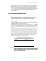
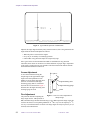
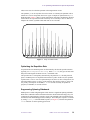
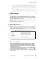
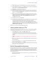
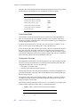
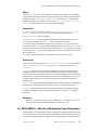
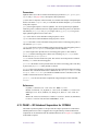
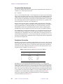
Finer adjustment and evaluation of the homogeneity is possible using a sample of solid
adamantane (not available from Varian). A linewidth between 2 and 10 Hz is typically
attainable, as shown in the sample spectrum in Figure 2.
2.5 Adjusting the Magic Angle
Improper adjustment of the magic angle results in incomplete collapse of the chemical shift
anisotropy (CSA) pattern. For carbons with significant anisotropy, such as aromatics and
carbonyls, this can greatly affect the linewidth of the observed resonance. In general, once
01-999162-00 A0800
VNMR 6.1C User Guide: Solid-State NMR
22
Chapter 2. CP/MAS Solids Operation
lb=1.0
5.2 Hz
at=0.2
(LB=1.0, AT=0.2)
Figure 2. Typical MAS Spectrum of Adamantane
adjusted, the magic angle should stay fairly constant. However, this is not guaranteed. The
angle should be checked and adjusted as follows:
• When the probe is inserted in the magnet
• Every day or second day of continuing operation
• If linewidths in any particular sample are suspiciously large
Once typical values for the minimum linewidths are established for any particular
instrument, these values can be taken as a reliable indication of proper angle. Adjustment
of the angle is neither necessary nor desirable if the first measurement indicates that the
minimum linewidth has been achieved.
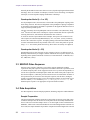
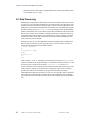
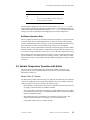
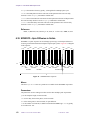
Coarse Adjustment
A convenient method of setting the
sample angle to the approximate magic
angle before final optimization with
NMR is to use the angle measuring stem
(Part No. 00-992825-00) and angle
measuring gauge (Part No. 00-99282600) from the rotor and tool kit. Figure 3
illustrates how the angle measuring stem
and angle gauge are used.
54.7°∞
54.7°
Angle measuring stem
Angle measuring gauge
Probe
Fine Adjustment
Figure 3. Tools for Coarse Adjustment of
The preferred method of adjusting the
Sample Angle
magic angle uses the 79Br spectrum of
KBr, which has a large chemical shift anisotropy (CSA). When spun at the magic angle, this
results in an extensive set of spinning sidebands. As 79Br is very close in frequency to 13C,
it is easy to switch between the two nuclei. The magic angle can easily be precisely set (or
checked) as described below.
23
VNMR 6.1C User Guide: Solid-State NMR
01-999162-00 A0800
2.5 Adjusting the Magic Angle
1.
Enter tn='Br79' to obtain the parameter set to observe 79Br.
If the following message appears
Requested nucleus, 'Br79' is not an entry in the nucleus
table nuctabXX
where XX is 2d, 3d, or 4d, then add this nucleus with the following VNMR
commands. Note that the first VNMR command invokes the vi text editor
(familiarity with this UNIX text editor is assumed).
vi('/vnmr/nuctables/nuctabXX')
Remember to use nuctab2d, nuctab3d, nuctab4d, or nuctab5d in place of
nuctabXX. Add one of the following lines above the Br81 line:
• For 200-MHz systems, add:
Br79
50.180 1.480e6
low yes 0.0
• For 300-MHz systems, add:
Br79
75.180 1.480e6
low yes 0.0
• For 400-MHz systems, add:
Br79 100.208 1.4842e6 low yes 0.0
Exit vi and then enter tn='Br79' again. No error should be generated.
2.
Load a rotor with KBr, insert in the probe, spin at 3 kHz, and tune the system for
79Br. Grinding the KBr crystals before packing the rotor is helpful.
3.
Set seqfil='s2pul' sw=1e5 at=0.02 nt=1. Enter ga to obtain a single
transient spectrum. Set the cursor on resonance, and enter movetof.
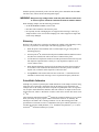
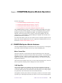
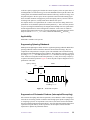
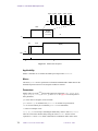
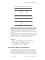
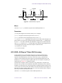
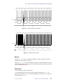
4.
Set phfid=0 and enter gf. Now open the acqi window, click the FID button,
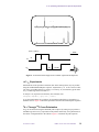
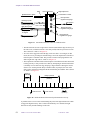
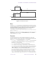
and observe the real-time FID display.
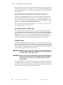
The FID displays a transient that is an exponential decay with a “picket fence” of
one or more spikes on it (see Figure 4 and Figure 5). If the signal is not exactly on
Figure 4. FID Display of KBr on Angle
resonance, adjust Z0 until it is, then select IPA and adjust phfid to maximize the
on resonance FID.
5.
Adjust the angle using the appropriate method below:
• Varian RT CP/MAS probes – Turn the screw between the two copper coax lines
in the probe baseplate.
• Varian VT CP/MAS probe – Turn the fiberglass rod with the adjustment tool.
• Doty CP/MAS probe – Turn the smaller gold rod.
01-999162-00 A0800
VNMR 6.1C User Guide: Solid-State NMR
24
Chapter 2. CP/MAS Solids Operation
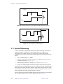
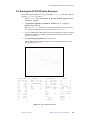
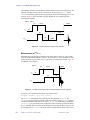
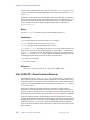
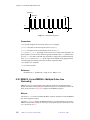
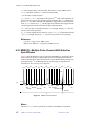
Figure 5. FID Display of KBr 1/2 Turn Off Angle
Maximize the size and number of spikes in the picket fence. The spikes should
persist for about 10 ms. The sample angle is now set to the magic angle.
6.
Close the acqi window and retune the probe to the appropriate nucleus.
The same sample and general procedure can be used to monitor spinning stability, both in
angle and in speed. An angular instability shows in two ways: the shape and size of the
exponential varies from transient to transient, and the picket fence is unstable in length and
amplitude if the rotor is vibrating.
Instability in the spinning speed can be measured by inspecting the summed FID. If
acquisition is continued for a time, the speed variation can be determined from the
broadening of pickets well down the fence in time. Run a four-transient FID and enter df.
With the FID now displayed, use cursors and related commands to edit the display. Measure
the resolution of a picket at the start and at the end of the FID display. Similar values
indicate good spinning stability.
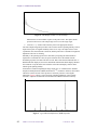
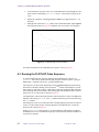
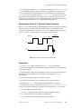
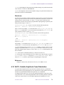
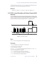
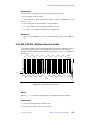
An alternative method of adjusting the magic angle uses 13C CP/MAS of the standard
sample, hexamethylbenzene (HMB), which has two 13C resonances. Of these, the aromatic
carbon line (on the left side of the spectrum) is extremely sensitive to the angular
adjustment. Figure 6 shows a typical spectrum, including sidebands, of the aromatic
resonance. Adjust the aromatic line for minimum linewidth and maximum intensity.
Figure 6. Typical Hexamethylbenzene (HMB) Spectrum
25
VNMR 6.1C User Guide: Solid-State NMR
01-999162-00 A0800
2.6 XPOLAR Pulse Sequence
Once typical values for the minimum linewidths are established for any particular
instrument, these values can be taken as a reliable indication of proper angle. Adjustment
of the angle is neither necessary nor desirable if the first measurement indicates that the
minimum linewidth has been achieved.
2.6 XPOLAR Pulse Sequence
The Varian-supplied XPOLAR (cross-polarization) pulse sequence is used to obtain CP/
MAS NMR spectra of solids. This sequence is used for most experiments. For more
information on the XPOLAR pulse sequence, see page 59 (UNITY systems) or page 63
(UNITYINOVA and UNITYplus)
2.7 Calibrating Pulse Width
The steps below provide instructions for calibrating the pulse width, as well as for
connecting the amplifiers and setting the parameters.
CAUTION:
To avoid severe damage to the probe, make sure that the values for the
parameters level1 and level2 do not exceed the values given for
maximum power for the probe.
1.
Insert a rotor containing p-dioxane and spin it at about 200 Hz.
2.
Record a spectrum using gated decoupling (dm='nny') and calibrate the 90° flip
time.
3.
Recall the parameters from parlib/xpolar and set
d1=5 nt=1 xpol='n' tpwr=45 tpwrf=4095. Vary pw.
If needed, you can create tpwrf with the following commands:
create('tpwrf','integer') setlimit('tpwrf',4095,0,1).
Depending on the probe, 90° pulse widths can range anywhere from 4.0 to 9.0 µs. The
observe transmitters can deliver up to 300 W for up to 20 ms (except on VXR-S). Develop
a matrix of tpwr and tpwrf values as they relate to pw90 and save the matrix for later
reference.
CAUTION:
Do not use more than 5% duty cycle for a pulse longer than 0.2 second
for the decoupler. For the standard XPOLAR pulse sequence, an error
message displays when the duty cycle reaches 20%. Refer to
individual probe data sheet for maximum pulse duration.
2.8 Calibrating Decoupler Power
Using the previously determined pw, calibrate decoupler power (γB2) as follows.
1.
Recall test parameters by entering rt('/vnmr/tests/hmb').
2.
Set dof=5e4,–5e4 d1=10.
3.
Set level2 and level2f such that the power output is about 80 watts.
4.
Enter ga.
01-999162-00 A0800
VNMR 6.1C User Guide: Solid-State NMR
26
Chapter 2. CP/MAS Solids Operation
5.
When acquisition is finished, measure the reduced coupling on each of the two
spectra.
CAUTION:
6.
To avoid damaging the probe, do not exceed the probe decoupler
power limit.
Enter h2cal to calculate γB2. If necessary, alter level2 to obtain a satisfactory
value of γB2.
2.9 Adjusting the Hartmann-Hahn Match
Hartmann-Hahn matching can be readily accomplished by using a sample of
hexamethylbenzene (HMB) or adamantane. These substances are not easily crosspolarized. However, they have a high degree of symmetry and so, once cross-polarized,
gives rise to very intense signals.
1.
Load a rotor with HMB or adamantane, insert it, and spin it slowly (about 2500 Hz
for HMB or 1800 Hz for adamantane). Adjust the spinning speed so that none of the
sidebands of the aromatic carbons overlap the methyl resonance.
2.
Recall the test parameters by entering rt('/vnmr/tests/hmb'). Set
xpol='y'. Set pw to a 90° 13C pulse. Set p2=2500 at=0.05 d1=4 nt=4.
3.
Set level2 and level2f as determined in the previous section and array
level1 to pass across the Hartmann-Hahn condition, with the value of level1
not to exceed level2. Enter a fixed value of gain, because Autogain cannot be
used in an arrayed experiment.
4.
Enter ga. When acquisition is finished, enter dssh to display the results. Select the
spectrum with the maximum signal and set level1 to the value +1 for this
spectrum (in the next step, we reduce level1f).
5.
Array level1f with the full range, 0 to 4000 in steps of 500.
6.
Enter ga, and when acquisition is finished, enter dssh. Select the value of
level1f that gives the maximum signal.
For an even closer match, array level1f in smaller steps around this value.
For systems equipped with an observe fine attenuator, tpwrf can also be used.
2.10 Optimizing Parameters and Special Experiments
This section provides information on parameters used for specific optimizations, such as
contact time and repetition rate. Also included in this section are special experiments for
the high-performance CP/MAS module. With each of these experiments is a sample
spectrum and an illustration of the XPOLAR pulse sequence used.
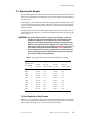
Contact Time Array
For samples in which cross-polarization is used, the “contact” time, that is, the time during
which cross-polarization occurs, must be optimized with the parameter p2. This is
necessary because two processes are occurring simultaneously:
• Build-up of magnetization due to cross-polarization
• Loss of magnetization due to rotating-frame relaxation
27
VNMR 6.1C User Guide: Solid-State NMR
01-999162-00 A0800
2.10 Optimizing Parameters and Special Experiments
Thus a time exists for which an optimum in the magnetization occurs.
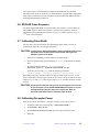
The optimum p2 can lie anywhere from 100 to 5000 µs. Generally the optimum value is
similar for a class of compounds, but for new types of samples an optimization of p2 is
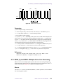
highly desirable. Figure 7 shows a typical optimization. Note that a simultaneous optimum
for all carbons in a spectrum does not necessarily occur. Generally a value of 1000 µs is
adequate for normal, crystalline solids and 3000 µs for soft solids.
Figure 7. Array of Contact Times
Optimizing the Repetition Rate
Acquisition times in CP/MAS spectra are determined by the desired spectral resolution.
Typically, set sw=300p (or sw=300*sfrq). With at=0.064, this gives at least 2048
data points and a digital resolution of 4 Hz, a reasonable value.
The repetition rate is consequently determined by the parameter d1, the delay between
pulses. CP/MAS spectra are acquired with 90° observe pulses. In this case, the optimum
repetition rate is 1.25*T1. For cross-polarization spectra, this T1 is the T1 of the protons; for
gated-decoupling spectra, it is the T1 of the carbon or other nucleus. These T1 values can
vary widely, as in liquids. At 300 MHz, a d1 of 5 seconds is usually acceptable for
polymers; at 400 MHz, 10 seconds is better.
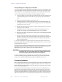
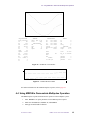
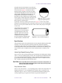
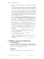
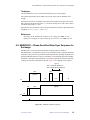
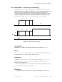
Suppressing Spinning Sidebands
NMR spectra of solids at high magnetic fields often have significant spinning sidebands.
While these sidebands contain information about the chemical shift anisotropy, they can
complicate the interpretation of complex spectra. The sidebands can be eliminated using
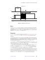
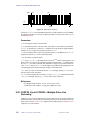
the TOSS (TOtal Sideband Suppression) technique. The TOSS pulse sequence is selected
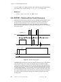
by setting toss='y' in the XPOLAR sequence (see Figure 8). Note that the parameter
srate should be set to the spinning speed in Hz.
01-999162-00 A0800
VNMR 6.1C User Guide: Solid-State NMR
28
Chapter 2. CP/MAS Solids Operation
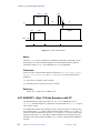
toss='y'
toss='n'
xpol='y' toss='y'
pw
1
H
level2
level1
d1
p2
13
C
Delay recipe
including srate
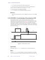
Figure 8. TOSS Experiment on Alanine (Spectrum and Sequence)
TOSS is less effective at high spinning speeds. Note that if suppression is not finished,
check that srate is correct. TOSS uses 180° pulses based on pw. It may be necessary to
adjust pw to optimize the TOSS experiment.
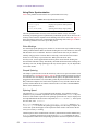
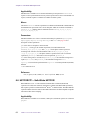
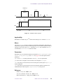
Suppressing Protonated Carbon (Interrupted Decoupling)
Off-resonance decoupling and related experiments in which J-coupling is involved are not
routinely possible in solids because dipolar coupling as well as J-coupling is present. One
experiment exists, however, that is used in solids to discriminate between carbon types, and
that is the protonated carbon suppression experiment of Opella and Fry. In this experiment,
the decoupler is turned off for 40 to 100 µs before acquisition to dephase the protonated
carbons.
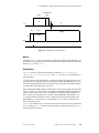
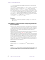
The technique is effective primarily for non-mobile carbons; mobile carbons, like methyl
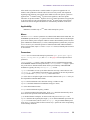
groups, are typically not suppressed as well. Figure 9 shows a typical protonated carbon
suppression experiment on alanine, obtained by setting pdp (protonated dephasing) equal
to 'y', setting srate to the spinning speed, and entering appropriate values for d2 (in
seconds), the dephasing time.
29
VNMR 6.1C User Guide: Solid-State NMR
01-999162-00 A0800
2.10 Optimizing Parameters and Special Experiments
pdp='y'
pdp='n'
xpol='y' pdp='y'
level2
pw
1
H
level1
d1
p2
13
2*pw
d2
C
1/srate
1/srate
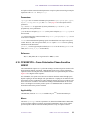
Figure 9. Protonated Carbon Suppression of Alanine (Spectrum and Sequence)
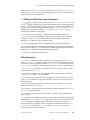
13C T
1ρ
Experiments
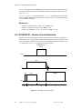
Measurements of the spin-lattice relaxation time in the rotating frame (Tlρ) are possible
using the standard XPOLAR pulse sequence. Anytime that p3 is set to a non-zero value,
a Tlρ decay is introduced; thus, by setting p3 to an array, Tlρ is measured. Typical values
for p3 would range from 50 to 5000 µs.
To analyze a Tlρ experiment for the decay time constant, enter
analyze('expfit','p3','t2','list')
or use the menu buttons for T2 analysis. In experiments other than Tlρ experiments, p3
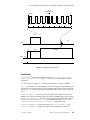
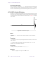
should be set to 0. Figure 10 shows the spin-lattice relaxation measurement pulse sequence.
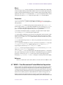
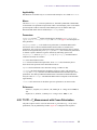
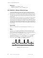
1H T Through 13C
1
Cross-Polarization
lH T
1
can be measured using the XPOLAR pulse sequence by setting it up to perform a
standard inversion-recovery experiment on the protons followed by cross-polarization of
the remain 1H magnetization to the carbons. Figure 11 illustrates the pulse sequence.
01-999162-00 A0800
VNMR 6.1C User Guide: Solid-State NMR
30
Chapter 2. CP/MAS Solids Operation
xpol='y'
pw
1
H
d1
p3
p2
13
level2
level1
C
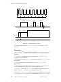
Figure 10. Rotating-Frame Spin-Lattice Relaxation Measurements Sequence
xpol='y'
level2
pw
p1
1H
d1
level1
d2
p2
13
C
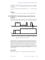
Figure 11. Pulse Sequence for Measuring lH T1
2.11 Spectral Referencing
A variety of methods are found in the literature for spectral referencing. Some involve a
small sealed capsule of TMS centered in the sample. Others use a small piece of
polyethylene as a secondary reference. For most purposes, primary and secondary
referencing are not necessary, and external secondary spectral referencing can be used as
follows:
1.
Insert a standard sample (e.g., HMB).
2.
Obtain a spectrum and set spectral referencing. (For HMB, set the cursor on the
aromatic line and enter rl(132.1p)).
3.
Adjust the display window as desired (for 13C, enter wp=200p sp=0).
4.
Remove the standard sample and insert the sample of interest. Obtain a spectrum.
Both field drift and field shifts affect this type of referencing. Field drift is typically small
and can be ignored. Field shifts due to magnetic susceptibility effects are finite but small.
Chemical shifts measured as described above are in all cases reasonable, but for a series of
similar compounds, the relative chemical shifts are even better.
For most purposes, this procedure should be followed only at the time the probe is installed.
The 13C chemical shifts of a few reference materials are given in Table 3.
31
VNMR 6.1C User Guide: Solid-State NMR
01-999162-00 A0800
2.12 Further Reading on Solid-State NMR
The setref command adjusts
referencing so that the solvent
frequency is correct, even when no
reference substance is present in the
sample.
setref uses absolute resonance
frequencies as defined in a file /
vnmr/nuctables/nuctabref;
currently, about 25 of the most
common nuclei are covered in this file.
setref can easily be expanded to
cover any other nucleus as well; a
recipe on how to expand setref is
given in the header of the file /vnmr/
nuctables/nuctabref.
Table 3. Reference Materials and 13C
Chemical Shifts
Substance
Chemical shift (ppm)
adamantane
29.2, 38.3
delrin
88.5
glycine
43.6, 176.4
hexamethylbenzene
17.3, 132.1
poly(methyl
methacrylate)
19, 45, 51, 176
talc (29Si)
–90
2.12 Further Reading on Solid-State NMR
General Sources on Line Narrowing in Solids
Gray, G. A.; Hill, H. D. W. Industrial Res. and Dev. 1980 (March).
Miknis, F. P.; Bartuska, V. J.; Maciel, G. E. Am. Lab. 1979 (November).
Griffin, R.G. Anal. Chem. 1977, 49, 951A.
Fyfe, C. A. Solid State NMR for Chemists. CFC Press: Guelph, 1983.
Cross-Polarization Technique
Pines, A.; Gibby, M. G.; Waugh, J. S. J. Chem. Phys. 1973, 59, 569.
Stejskal, E. O.; Schaefer, J.; Waugh, J. S. J. Magn. Reson. 1977, 28, 105.
Relaxation Times
Schaefer, J.; Stejskal, E. O.; Buchdahl, R. Macromolecules 1977, 10, 384.
Spinning Sidebands
Herzfeld, J.; Berger, A. E. J. Chem. Phys. 1980, 73, 6021.
Dixon, W. T. J. Magn. Reson. 1981, 44, 220.
Dixon, W. T. J. Magn. Reson. 1982, 49, 341.
Dixon, W. T. J. Magn. Reson. 1985, 64, 332.
Protonated Carbon Suppression
Opella, S. J.; Fry, M. H. J. Am. Chem. Soc. 1979, 101, 5856.
Frye, J.; Maciel, G. E. Magical Angle Adjustment with KBr. J Magn. Res. 1980.
01-999162-00 A0800
VNMR 6.1C User Guide: Solid-State NMR
32
Chapter 2. CP/MAS Solids Operation
2.13 Useful Conversions
Convert from 90° pulse width to γH:
250
γ H 2 ( kHz ) = -------------------------------------- ( µs )
90°pulsewidth
Convert from field strength in gauss to field strength in gauss:
1H: γH (kHz) ≈ 4.3 * γH (gauss)
13C: γH (kHz) ≈ γH (gauss)
Convert from rf fields to power levels:
P (watts) ∝ (γH)2
33
VNMR 6.1C User Guide: Solid-State NMR
01-999162-00 A0800
Chapter 3.
Wideline Solids Module Operation
Sections in this chapter:
• 3.1 “Wideline Solids Module,” this page.
• 3.2 “Wideline Experiments,” page 38.
• 3.3 “SSECHO Pulse Sequence,” page 39.
• 3.4 “Data Acquisition,” page 39.
• 3.5 “Standard Wideline Samples,” page 41.
• 3.6 “Data Processing,” page 43.
Unnarrowed spectra of solid samples can often reveal a great amount of information. In
wideline NMR, no attempt is made to narrow the resonances (as done by CP/MAS), and
patterns up to 0.5 MHz or wider can occur.
As lineshape is of the utmost importance, the spectrometer must be able to measure very
broad lines without any distortion. It is for this reason that the transmitter power is high.
γH1 must be large enough to uniformly excite the entire spectrum. (The effects of a finite
90° pulse width may be investigated with simulations using the solids analysis software
accessory.) With linewidths in excess of 100 kHz, an increase in ADC speed is necessary.
In fact, the typical spectral widths used often greatly exceed the linewidths because many
spectra are obtained under over-digitized conditions.
3.1 Wideline Solids Module
The wideline module for the Varian spectrometer modifies and extends the basic capability
of the system in a number of areas. The main components of the wideline module are the
wideband ADC, high-power amplifier, and the solids cabinet.
Wideline ADC Board
A wideline analog-to-digital conversion (ADC) board is added to the system in addition to
the standard ADC board. Based on the spectral width (the parameter sw), the software
determines which ADC board is to be used—values of sw greater than 100 kHz will
automatically use the faster ADC.
Two versions of the wideline ADC board exist:
• The newer version of the Wideline ADC board (Part No. 00-993350-00) was shipped
with UNITYplus systems. It has its own on-board memory, which consists of 2 x 64
Kword buffers (maximum np is 131072), together with its own sum-to-memory
(STM) circuitry. Data is summed at this speed without additional overhead. This board
also contains a Bessel filter, either 256 kHz (6-pole Bessel) or 1 MHz (4-pole Bessel).
This filter is switched in when sw is less than 256,000 Hz; otherwise, the 1 MHz filter
on the receiver is used.
01-999162-00 A0800
VNMR 6.1C User Guide: Solid-State NMR
34
Chapter 3. Wideline Solids Module Operation
• The older Wideline ADC board was shipped with UNITY and VXR-S systems. It
acquires data in a fundamentally different manner. Data is temporarily stored in its onboard, 2 x 8 Kword buffer (maximum np is 16384). After each FID is collected, data
is transferred to the normal acquisition memory and the fast memory is cleared. This
process requires an overhead of about 32 µs for each complex point.
Both ADC boards are single VERSAbus boards containing sample-and-hold modules,
ADC chips, memory, and control logic, and each board is capable of digitizing 12 bits in
500 ns. The ADC conversion time is adjustable in 25 ns steps, so there are only a limited
number of actual values that the spectral width can take. The entered value of sw is
automatically adjusted to the nearest valid spectral width.
The standard Observe Receiver board for UNITYINOVA and UNITYplus systems has the
correct bandwidth amplifier and is not replaced. For UNITY and VXR-S systems, the
Wideline Receiver and Filter board is a replacement of the standard 100 kHz receiver and
contains filters appropriate for both small and large spectral widths. Improved filters give
better baseline and phase characteristics; however, they may show a 10% reduction in
signal-to-noise as determined by the standard 13C test.
For spectral widths above 100 kHz, 6-pole true
Bessel filters are used. The outputs from these
filters are routed to the wideband ADCs. The
permissible values of the parameter fb, which are
identical to the 3 dB points of these filters, are
listed in Table 4.
For 100 kHz and below, the signal is routed
through a pair of 8-pole quasi-elliptical filters to
standard ADCs. The characteristics of these filters
provide superior performance for both phase and
amplitude flatness across the full spectral width.
Table 4. Bessel Filter Outputs
sw (kHz)
fb (kHz)
100 – 225
256
> 225
1000
300 – 540
300
540 – 1260
700
1260 – 1800
1000
> 1800
2400
The Wideline NMR Module for the UNITYINOVA
system is a board that includes two 5-MHz 12-bit ADCs and 2 MB of onboard memory.
High-Power Amplifier
The wideline high-power (1 kW) amplifier is intended mainly for use in solid-state NMR
studies. The amplifier is housed in a third cabinet, as shown in Figure 12, and configured to
permit maximum flexibility. Manual controls permit selection of either the solids amplifier
or the standard liquids amplifier for the observe function.
CAUTION:
Never use probes designed for liquids studies with amplifiers intended
for solid-state studies. The high power from these amplifiers will
destroy liquids probes.
Because the wideline package is for low-band (12 to 200 MHz) nuclei, no 1H or 19F highpower amplifier is provided unless the CP/MAS module or CRAMPS/Multipulse module
is also installed. The 1-kW power amplifier is one of the following models:
• The AR Model 1000LPM10 covering the range of 9 MHz to 200 MHz with 60 dB of
gain and a maximum output power exceeding 60 dBm over this range.
• The AMT Model M3201 covering a range of 6 MHz to 220 MHz with 10 dB of gain
and a maximum power output exceeding 60 dBm over this range.
35
VNMR 6.1C User Guide: Solid-State NMR
01-999162-00 A0800
3.1 Wideline Solids Module
Status panel
Sorensen Solids
VT controller (optional)
Low band 1 kW
amplifier
Low band
power supply
High band 1 kW
amplifier
High band
EHT power supply
Figure 12. Solids Cabinet Layout, Open Front View
Both amplifiers are linear, with gating provided for noise blanking. Operational details for
the high-power amplifiers are included in the manuals provided by the manufacturers of the
amplifiers. These should be read before operating the amplifier.
AR Linear Amplifier
The AR linear amplifier is gated off whenever the receiver is gated on. A time of at least 30
µs is required for the bias to come on fully and thus for the amplifier to provide full output
power. Allowance for this delay must be made in any pulse sequence programming, using
rof1. The amplifier can be driven in either of two modes:
• Continuous wave (CW)—the maximum power output is limited to 200 W but the duty
cycle can be 100%
• Pulsed—the maximum power output is 1 kW but the maximum pulse width is 8 ms
with a maximum duty cycle of 10%.
The amplifier is fully protected against thermal overload, excessive duty cycle, and
excessive pulse width. Status lights on the front panel and switches for this unit are visible
by opening the front door of the third cabinet.
01-999162-00 A0800
VNMR 6.1C User Guide: Solid-State NMR
36
Chapter 3. Wideline Solids Module Operation
Although you should study the AR manual before using the amplifier, an abbreviated set of
operating instructions are given here (words in all capital letters refer to controls on the
front panel).
The gating input to the amplifier is of positive logic, with a 5 V on and 0 V off signal. The
amplifier is class A with noise blanking in the CW mode. In the pulsed mode, the amplifier
operates class AB and the gating input acts as a gating signal. When gated off, the output is
greatly attenuated.
• To operate in the continuous mode, turn on the POWER button, wait for the
STANDBY button to light, then press the OPERATE button. In the continuous mode,
the gating signal input should be disconnected at the AR front panel.
• To operate in the pulsed mode, press the OPERATE button to set the amplifier in the
standby mode. Press the PULSED button, then the OPERATE button once again. The
amplifier is now in the pulsed mode, with pulse gating, not noise blanking. The
maximum rated power output in the pulsed mode is 1 kW (60 dBm). This should not
require adjustment of the amplifier gain.
• To return to the continuous mode, switch back to the standby mode by pressing the
OPERATE button, followed by powering off the amplifier.
The AR amplifier has been calibrated at 100 MHz so that when its front panel gain control
is set to the marked position and the manual attenuators are set to 0, the power output is
equal in dBm to the value of tpwr, in other words, tpwr=60 delivers 1 kW (60 dBm) and
tpwr=50 delivers 100 W (50 dBm). This calibration may not be precise at other
frequencies, but provides a first approximation.
AMT Linear Amplifier
The AMT linear amplifier is gated off whenever the receiver is gated on. A time of at least
8 µs is required for the bias to come on fully and thus for the amplifier to provide full output
power. Allowance for this time delay must be made in any pulse sequence programming,
using rof1.
The maximum pulse width is 20 ms at full output and with a maximum duty cycle of 10%.
The AMT amplifier is fully protected against thermal overload and it indicates excessive
duty cycle and excessive pulse width. Status lights on the front panel and the power switch
are visible inside the front door of the third cabinet as well as on the status panel. The gating
input to the amplifier is of positive logic, with a 5 V on and 0 V off signal.
CAUTION:
Never operate a high-power amplifier unless terminated by an
appropriate 50-ohm load.
Decoupler Amplifier
The three possibilities for the decoupler amplifier in wideline systems are as follows:
• Standard decoupling operation.
• 100 W CP/MAS decoupler—operation of this is the same as for CP/MAS.
• 1 kW decoupler amplifier.
Status Panel
The high power amplifiers are controlled by a status panel.
The HI POWER ENABLE subpanel contains two switches:
37
VNMR 6.1C User Guide: Solid-State NMR
01-999162-00 A0800
3.2 Wideline Experiments
• The OFF button grounds the inputs of both high power amplifiers and routes the
transmitters through the standard UNITYINOVA, UNITYplus, and UNITY electronics
appropriate for liquids operation (note that both amplifiers are left powered up by this
switch).
• If HI POWER ENABLE is OFF, the position of the HI POWER/LO POWER switch
is immaterial—the high-power amplifiers cannot receive any rf drive. The ON switch
activates the cabinet, enabling the HI POWER/LO POWER toggle switches.
Observe Transmitter
For both the solids and standard liquids channels, the computer-controlled attenuators are
in-line. The power level is controlled by the parameter tpwr in 1 dB increments from –16
to 63 dB standard (0 to 63 dB is standard on UNITY and VXR-S systems). Maximum
power output is obtained with tpwr=63. To get low power from the high-power amplifier,
tpwr should be decreased by approximately 6.
Note that the output of the Observe Transmitter board can be routed to a low-power (300
W) amplifier (LOW POWER position on the third cabinet, see Figure 12) or to a highpower (1 kW) amplifier (HI POWER position).
3.2 Wideline Experiments
Wideline NMR experiments can be divided into three main areas, based on spin quantum
number (I). The experiments possible are certainly not restricted to just one of these
categories, but are normally used in one group rather than in all. Table 5 lists commands
and parameters related to wideline experiments.
Table 5. Wideline Experiment Commands and Parameters
Commands
ssecho
tmove
tshift
Set up solid-state echo pulse sequence
Left-shift FID to time-domain cursor
Adjust tau2 to current cursor position
Parameters
dotflag {'y', 'n'}
lsfid {number, 'n'}
scalesw {number > 0.0, 'n'}
Display FID as connected dots
Number of complex points to left-shift np
Scale spectral width in directly detected dimension
Dipolar Nuclei (I = 1/2)
The most common dipolar nucleus is 1H. Many of the dipolar nuclei are not usefully
observed under wideline conditions without 1H decoupling. Although the standard
wideline probe does not allow double-resonance experiments, a CP/MAS probe can be
used for many such experiments.
In 1H wideline experiments, lineshape or chemical shift is usually of minor importance.
The most interesting parameters are relaxation rates such as T1, T2, and T1ρ. In many
measurements the relevant part is the first few microseconds of the FID. The FID may not
even be transformed.
01-999162-00 A0800
VNMR 6.1C User Guide: Solid-State NMR
38
Chapter 3. Wideline Solids Module Operation
Normally the breadth of a line comes from two sources, dipolar coupling and chemical shift
anisotropy. There are a number of techniques, referred to as line narrowing, or multipulse
techniques, to remove dipolar coupling contributions to lineshape.
Quadrupolar Nuclei (I = 1 or 3/2)
For all quadrupolar nuclei, the main cause of linewidth is the quadrupolar coupling of the
nuclei being observed. The observed magnitude of the quadrupolar coupling is dependent
on orientation in the magnetic field and is responsible for the apparent difference between
single crystal and powder spectra.
The most commonly observed quadrupolar nucleus in wideline is 2H (deuterium), along
with 23Na and a few other nuclei. Lineshape is of prime consideration in most experiments
involving these nuclei, with relaxation measurements also of interest.
To ensure an accurate representation of the lineshape, most spectra are measured via an
echo sequence, first described by Mansfield (Phys. Rev., 137, A961, (1965)), commonly
known as the “solid echo” sequence. To simplify phasing of the transformed FID, the echo
is Fourier transformed from the top onwards in time. The “extra” data points are ignored
using lsfid. To accurately define the echo top, these echoes are usually over-digitized.
Quadrupolar Nuclei (I > 3/2)
Quadrupolar nuclei are also observed via echo sequences; however, as different types of
lineshape information may be sought, a number of different echo sequences may be used,
depending on the quantum transitions of interest (I. D. Weisman and L. H. Bennett, Phys.
Rev., 181, 1344, (1969)).
3.3 SSECHO Pulse Sequence
One basic pulse sequence, SSECHO, is provided to support quadrupolar wideline
experiments. This pulse sequence can perform conventional “solid echo” experiments, with
or without composite pulses. It also supports inversion-recovery solid echo experiments, as
well as echo experiments with unequal pulse widths. The details of this pulse sequence are
discussed in Chapter 6, which also provides a model for users for whom other variations of
the experiment may be of interest. Since this pulse sequence, like all others, undergoes
periodic revision and improvement, you are encouraged to print the version current in your
software with the ptext command: ptext('/vnmr/psglib/ssecho.c'). The
SSECHO pulse sequence is not appropriate for proton relaxation studies.
3.4 Data Acquisition
For data acquisition, consider sample preparation, shimming, and pulse-width calibration.
Sample Preparation
The main requirement is that the sample be no longer than 25 mm nor greater than 5 mm
in diameter. Samples must fit into the coil of the probe and be electrically insulated from
the coil. The most convenient sample carrier is a 15 mm length of 5 mm outside diameter
NMR tube, which can be sealed with Parafilm or some other background-free material. For
best results, the sample should be kept small in comparison with the length of the coil and
39
VNMR 6.1C User Guide: Solid-State NMR
01-999162-00 A0800
3.4 Data Acquisition
should be placed symmetrically in the coil when in the probe. Remember that the NMR
tube has a 29Si, (l3Na)27Al and 11B background signal.
WARNING: Dangerous high voltage exists inside the probe that can cause burns
or serious injuries. Follow the instructions below to avoid the hazard.
When changing samples, take the following precautions:
• Set the HI POWER ENABLE switch to OFF.
• Disconnect the transmitter cable from the probe.
• Be especially careful of damaging the coil supports when inserting or removing a
sample from the coil as well as when changing coils. These supports are fragile and
can be easily damaged.
Shimming
Because of the width of the resonances encountered in wideline work, shimming is rarely
necessary (or possible!) on each sample. The following approach is typical:
1.
When the probe is first installed, insert a sealed sample of D2O in the probe for
shimming purposes.
2.
Tune the probe to 2H, as described in the probe installation manual, and then connect
the (otherwise unused) lock cable to the observe channel of the probe.
3.
Use the interactive acquisition window to lock the spectrometer in the usual way, and
then adjust the important shims. Usually it is only important to adjust X, Y, Z1
Coarse, and Z2 Coarse.
4.
When finished shimming, turn the lock off and adjust Z0 so that the lock signal is
on-resonance. This ensures that the field will be in the same position as used for
liquids work, so that the usable frequencies will be the same.
5.
Set lpower=0. This ensures that at the time of the next su command, the lock
transmitter is deactivated, removing a source of potential frequency interference.
Pulse-Width Calibration
Although it is possible to perform pulse width calibrations on the sample of interest using
solid-state echo experiments, calibrations done in this manner can be misleading. For
example, there is not usually a null at the 180° pulse for quadrupolar nuclei. As a general
rule, all pulse width calibrations should be made with solutions. A sample of D2O can be
used for 2H work, while a 1 M solution of a salt in water can be used for other nuclei such
as 23Na.
The acquisition controller board of the UNITYINOVA has a timing resolution of 12.5 ns, which
limits your ability to specify a pulse width to increments of 0.0125 µs. Similarly, the
UNITYplus and UNITY have a timing resolution of 25 ns, thus limiting pulse width
specification to increments to 0.025 µs. Adjustment of the power with the parameter tpwr
will alter the 90° pulse width parameter pw90. In addition, the parameter tpwrm can be
used with UNITYINOVA and UNITYplus systems.
01-999162-00 A0800
VNMR 6.1C User Guide: Solid-State NMR
40
Chapter 3. Wideline Solids Module Operation
3.5 Standard Wideline Samples
Two standard wideline samples are provided with the system, malonic acid-d4 for 2H and
sodium nitrate for 23Na wideline NMR. These samples are provided as an aid to becoming
familiar with the operation of the wideline module and do not have any associated
specifications.
Obtaining a Wideline Spectrum of Deuterium
The deuterium powder pattern spectrum of malonic acid-d4 can be obtained in the
following manner (this is not the only way to operate the wideline module, but does provide
a convenient starting point):
1.
Determine the 90° pulse using a solution, in this case, 2% D2O (for most other
quadrupolar nuclei, a 1 M solution of a salt in water should be used). Put the relevant
tuning rod into the probe. Connect the correct coil in the correct pair of connectors
on top of the probe body. Refer to the probe installation manual for details on setting
up the wideline probe.
2.
Place a sealed sample of 2% D2O in the probe and put the probe into the magnet.
Connect body air, VT gas and the “Normal” connector on the magnet leg to the
probe. No filters are necessary. Make sure that the 30–60 MHz 1/4-wavelength cable
is on the magnet leg.
3.
Enter setup('H2','d2o') dm='n' su. Tune the probe as described in the
probe installation manual.
4.
Now, instead of the observe channel, connect the lock channel to the probe. Lock the
spectrometer in the usual way.
The spectrometer can now be shimmed using acqi, but there is no point trying to
obtain a resolution that is markedly better than the lines to be observed, so that only
the gradients X, Y, Z1 Coarse, and Z2 Coarse need be optimized.
5.
Make sure that the lock and spinner are deactivated by selecting LOCK OFF, SPIN
OFF, SPIN=0 and setting lockpower=0.
6.
Replace the lock connection with the observe channel. Check the tuning and then
make sure that the probe is connected to the “Normal” position on the preamplifier.
7.
If not already done, reset the solids cabinet, and make sure the broadband 1 kW
amplifier is on and that no interlocks are activated. Set the switch panel so that the
LOWBAND is on HI POWER.
8.
Set sw=1E5 pw=2 np=1E4 d1=4 nt=1. Set tpwr to the standard value for the
system. If no value has been determined previously, set tpwr=55.
9.
Set gain='n' and acquire a spectrum. Phase correct the result and ensure that the
spectrometer is working correctly. If necessary, use movetof to place the D2O
signal exactly on resonance.
10. Check these adjustments by reacquiring a spectrum.
11. Array pw to determine the 180° or 360° pulse width. Set gain='y' (because
arrayed experiments cannot use Autogain) and acquire the data. Determine the 90°
pulse width to 25 ns resolution.
12. Set pw and pw90 to the 90° pulse width value.
This completes the calibration procedure.
41
VNMR 6.1C User Guide: Solid-State NMR
01-999162-00 A0800
3.5 Standard Wideline Samples
13. Replace the D2O sample with the malonic acid–d4 sample and tune the probe.
14. Enter ssecho to convert the s2pul parameter set to one suitable for the SSECHO
pulse sequence. Set tau1=20 tau2=15 nt=16.
15. Set gain='n' and enter go to acquire data.
16. Enter df to display the FID. Use the phase button and the mouse to maximize the
real (cyan) channel. Set lsfid=0. Put a single cursor on the echo maximum and
enter tmove. Transform the FID.
17. Phase correct the spectrum using rp only (set lp=0). Select two cursors and set
each on top of a horn of the powder pattern. Enter split to move the right cursor
to half way between the two horns. Entering movetof then sets the observe
transmitter to this position.
18. Reacquire data, this time with d1=10.
19. Enter df to isplay the FID. Maximize the real channel as in step 16 and put a single
cursor at the echo maximum, putting it between data points if necessary.
This FID can either be transformed or data reacquired starting from the cursor
position. If the FID is to be transformed, then enter tmove wft. Phase correct the
spectrum as before. If new data is to be acquired starting at the cursor position, enter
tshift followed by go or ga.
Other spectra can now be acquired using these parameters.
Obtaining a Wideline Spectrum of 23Na
Sodium does not normally have a parameter set in stdpar, so it is necessary to call up
some standard set and modify it. The easiest way to do this is shown in step 1 below.
1.
Enter setup('H2','d2o') tn='Na23' dm='n' su.
2.
Set up the probe with the correct coil and tuning rod (if any) and put in a sealed
sample of NaCl (1 M in H2O). Tune the probe as described in the probe installation
manual.
3.
Follow step 5 through step 12 in “Obtaining a Wideline Spectrum of Deuterium,”
page 41.
4.
Remove the sealed sample of NaCl (1 M in H2O) and replace it with the sample to
solid sodium nitrate.
5.
Tune the probe and enter ssecho to convert to the QUADECHO sequence and
acquire 16 transients using a d1 of 1 second.
6.
Process the spectrum the same as for deuterium, except that the center of the powder
pattern is the center of the highest line.
Hints for Performing Wideline Experiments
If a powder pattern shows more than 3-4% asymmetry in the height of the horns, check that
the sample is centered in the coil. If this is the case, check the tuning of the probe. If neither
results in a significant improvement, shift the transmitter position 1000 Hz towards one
horn. Finally, recalibrate the 90° pulse with a solution sample, then retune the probe to the
same reflected power level.
• T1 can be very long in solids. It may be necessary to set d1 to values of the order of
100 seconds in some cases.
01-999162-00 A0800
VNMR 6.1C User Guide: Solid-State NMR
42
Chapter 3. Wideline Solids Module Operation
• Remember that for solid samples of quadrupolar nuclei, the 90° pulse usually cannot
be determined from a pw array.
3.6 Data Processing
Most data processing needs of wideline spectra are the same as that for other spectra. There
are, however, several specialized applications, for which software is provided. Since most
wideline spectra are collected in a spin-echo mode, it can be extremely important to start
acquisition, or at least Fourier transformation, on top of the echo. The FID display program
provides a point-by-point (if dotflag='y'), two-color display of the real and imaginary
channels of the FID in order to provide the best possible examination of the details of the
FID. One or two time cursors can also be displayed and are not constrained to fall on top
of individual data points but may be used to interpolate as well (for example, to estimate
the time of the echo). A left shift of the FID may be used to shift the FID until the echo
occurs at the first point of the FID.
Normally, the echo top is well enough defined so that left shifting removes all distortion.
However, this is not always the case, especially with very short T2 echoes. A means of
fractionally left shifting has been provided as follows:
lsfid='n' phfid='n'
ft
ft('inverse',n,expn)
jexpn
scalesw=1.0/n
df
wft
In this example, n in the ft command is a interpolation factor (power of 2); expn is an
experiment number for the interpolated FID; df interpolates the FID by a factor of n and
the echo top may be picked more accurately; scalesw=1.0/n will correct sw.
It is also common to collect wideline spectra with the transmitter placed in the exact center
of the resonance. Software is provided to allow “phasing the FID” to place as much as
possible of the FID in the real channel. This operation means that the frequencyindependent phase shift of the spectrum is as close to zero as possible, which is beneficial
since frequency-domain phasing of wideline spectra can be difficult at best. In addition,
spectral symmetry can be forced by software that sets the imaginary channel of the FID to
zero.
43
VNMR 6.1C User Guide: Solid-State NMR
01-999162-00 A0800
Chapter 4.
CRAMPS/Multipulse Module Operation
Sections in this chapter:
• 4.1 “CRAMPS/Multipulse Module Hardware,” this page.
• 4.2 “Running the FLIPFLIP Pulse Sequence,” page 46.
• 4.3 “Running the FLIPFLOP Pulse Sequence,” page 47.
• 4.4 “Using MREV8 to Demonstrate Multipulse Operation,” page 48.
The CRAMPS/multipulse module is available for 300-MHz and 400-MHz spectrometer
systems. It provides wideline capability for 1H and 19F, including the ability to perform
multipulse experiments such as MREV8 and BR24. The standard liquids high-band
amplifier is boosted to an upper limit of 1 kW by a tuned, linear amplifier. The main
components are a wideband ADC, high-band high-power amplifier, fine attenuator, and
pneumatics/tachometer control box.
For UNITY and VXR-S systems, the sync module is used to synchronize acquisition to the
master clock. Also, the liquids observe receiver is replaced by a wideband observe receiver,
described in “Wideline Solids Module,” page 34.
4.1 CRAMPS/Multipulse Module Hardware
The main CRAMPS/multipulse module hardware is the motor control box, 1-kW amplifier,
sync module (UNITY and VXR-S systems only), and the CRAMPS probe.
Motor Control Box
The motor control box is used to adjust the output load and tuning of the 1 kW proton
amplifier (see below). It consists of a selector switch with 3 positions—TUNE, LOAD and
STANDBY (or AUX)—and two 3-position toggle switches, COARSE and FINE. The
toggles are momentary contact and can be pushed sideways in two directions (which are
designated IN and OUT).
The box moves the end plates of the cavity in or out to affect the tuning process. In each of
the active positions, the plate position is displayed on a meter on the box.
1-kW Amplifier
The decoupler amplifier uses an EIMAC cavity tube. Thus the amplifier has both lowvoltage power supplies and a high-voltage supply. The high-voltage power supply (EHT) is
2.3 kV and is produced by the unit in the bottom of the solids cabinet. Low-voltage supplies
are produced by a unit in the bottom of the cabinet behind the EHT.
The amplifier is tuned by three controls to the frequency at which it is to be used. It is able
to produce up to 1 kW output for periods up to 250 ms, or lower levels for longer periods.
01-999162-00 A0800
VNMR 6.1C User Guide: Solid-State NMR
44
Chapter 4. CRAMPS/Multipulse Module Operation
The amplifier runs in a linear mode and can be considered to be a gain stage added to the
liquids high-band amplifier. The 1 kW stage operates in either blanked or unblanked modes
in exactly the same manner as its low-power driver. It should never be driven by more than
50 W (47 dBm).
Three controls are used to tune the amplifier: INPUT TUNING, on the front of the
amplifier, and OUTPUT TUNE and LOAD, on the remote motor control box.
When used for CRAMPS/Multipulse in the observe transmit chain, the amplifier is run
blanked, rather than unblanked as in CP/MAS. As a result, sufficient unblanking time
(rof1) must be allowed for the amplifier to turn on. The whole transmit amplifier chain
requires a rof1 of 1.5 (µs) for this. The reblanking time is very short, so that rof2 can be
set to zero. These timings ignore any probe ring-down issues.
If the system is equipped with 6-dB fine attenuators, tpwrf and tpwr must be set and
used, whether high power is selected or not.
Sync Module (UNITY, VXR-S only)
The sync module, located on the wideline receiver, provides a buffered 500-kHz signal
derived from the master oscillator. Its output is connected to the EXT TIMEBASE input on
the output board. A pulse sequence can delay until the next clock edge by using the pulse
sequence element xgate(1.0) at an appropriate point. This is commonly used in
multipulse sequences to improve stability when running high-resolution experiments for a
long time. The VNMR User Programming Manual describes its use in more detail.
CRAMPS Probe
The standard CRAMPS probe has a VT range from –120° to +160° C and can typically tune
from the 19F frequency to that of 1H. It is optimized for 1H and is essentially background
free for that nucleus. In order to achieve low 1H background, many components are made
of a fluorocarbon, so that a high 19F background exists. This may not necessarily preclude
19F line narrowing experiments, but care must be taken.
WARNING: Dangerous high rf voltage in the system can cause serious injury or
death. To avoid electrical shock completely turn off rf and disconnect
all rf cables before removing the probe.
WARNING: Spinner rotors have very high kinetic energy and can disintegrate at
any time. To prevent possible cuts or blindness, wear a certified fullfaced safety shield and cover all exposed skin while observing a
rotating sample
The CRAMPS probe has a 5-mm rotor and is designed to spin to 8 kHz. The probe does not
have high sensitivity because sensitivity is not normally an issue in multipulse experiments,
where proton is an abundant spin. Where rare spin conditions apply, the damping box can
be removed, in which case the ring-down time will be longer.
45
VNMR 6.1C User Guide: Solid-State NMR
01-999162-00 A0800
4.2 Running the FLIPFLIP Pulse Sequence
4.2 Running the FLIPFLIP Pulse Sequence
The FLIPFLIP pulse sequence is set up by running the flipflop macro and setting the
parameter phase2 to 0, as follows:
1.
Enter flipflop and set d1=4 pw=1.5 fb=1e6 sw=2e6 np=128 tau=7
rof1=1.5 rof2=0.
2.
Set phase1=0 phase2=0 phaser=0 phfid=0 or 'n' trig='n'
gain=0 nt=1 dp='y'.
Note that trig='n' is needed for UNITYINOVA and UNITYplus systems because
the 500-kHz synching signal is not available; otherwise, set trig='y'.
3.
Acquire a FID and enter df to display both real and imaginary components. Adjust
the phase to minimize the imaginary signal. If this is not possible, check that the
signal is on resonance.
4.
Enter phaser=phfid phfid='n' and reacquire.
The imaginary channel should be minimal. The real channel should show a FID
pattern similar to Figure 13.
ACQUISITION
sfrq 399.952
tn
H1
np
128
sw
2e+06
fb
1e+06
bs
16
ss
0
tpwr
54
tpwrf
3500
pw
1.500
tau
3.500
d1
4.000
tof -2986.3
nt
1
ct
1
SAMPLE
date Apr 1 93
file
exp
DECOUPLING
dn
H1
dof
0
dm
n
dpwr
30
0
PROCESSING
lb
not used
sb
not used
gf
not used
awc
not used
lsfid
0
phfid not used
fn
4096
FLAGS
il
n
in
n
dp
y
trig
y
SPECIAL
srate
1542
temp
27.0
werr
wexp
wbs
wnt
FLAGS
ai cdc ph
tauc
10.000
mp_at 0.000640
df
phase1
phase2
phaser
0
0
0
Figure 13. Real Channel FID Pattern
01-999162-00 A0800
VNMR 6.1C User Guide: Solid-State NMR
46
Chapter 4. CRAMPS/Multipulse Module Operation
5.
Count the number of points in one cycle of the FID and the reestimate pw for a 90°
pulse from the relationship pw=pw * 4/n, where n is the number of points in one
cycle.
6.
Repeat the acquisition, adjusting pw and then tpwr to get approximately a 1.5 µs
90° pulse.
7.
Enter gf, then connect the acqi window. Select FID and then IPA. Adjust tpwrf
until a pattern similar to Figure 14 is obtained. This occurs at the exact 90° pulse.
Figure 14. FLIPFLIP FID at Exact 90° Pulse
For further information on the FLIPFLIP pulse sequence, refer to page 100.
4.3 Running the FLIPFLOP Pulse Sequence
To run the FLIPFLOP pulse sequence rather that the FLIPFLIP pulse sequence, set
phase2=2. This train of pulses alternately flips the spins into the XY plane—giving an
NMR signal—and back to the Z axis—giving no NMR signal.
This sequence is used for other adjustments in most CRAMPS/Multipulse spectrometers,
but because of the phase shifting circuit used in the UNITYINOVA and UNITYplus systems,
this sequence is only used to remove “phase glitch” caused by asymmetric phase transients
at the beginning and end of each pulse. The resulting FID of the FLIPFLOP pulse sequence
appears as a set of “tram tracks” as shown in Figure 15.
The adjustment to remove phase glitch is done either at the probe or at the 1 kW high band
amplifier. After setting phase2=2, enter gf and then interactively observe the FID, using
the acqi window.
If the FID shows a sine wave in the tram tracks, carefully adjust the probe tune or match to
remove it. If this cannot be done, carefully adjust the 1 kW amplifier tune or load. The
desired result is shown in Figure 16.
Finally, set phase2=0 and repeat the pw90 determination as outlined above, using the
FLIPFLIP process. No re-examination of gating is required, but the 90° pulse should be set
as precisely as possible.
47
VNMR 6.1C User Guide: Solid-State NMR
01-999162-00 A0800
4.4 Using MREV8 to Demonstrate Multipulse Operation
ACQUISITION
sfrq 399.952
tn
H1
np
128
sw
2e+06
fb
1e+06
bs
16
ss
0
tpwr
54
tpwrf
2794
pw
1.400
tau
10.000
d1
4.000
tof -2986.3
nt
1
ct
0
SAMPLE
date Apr 1 93
file
exp
DECOUPLING
dn
H1
dof
0
dm
n
dpwr
30
PROCESSING
lb
not used
sb
not used
gf
not used
awc
not used
lsfid
0
phfid not used
fn
4096
FLAGS
il
n
in
n
dp
y
trig
y
SPECIAL
srate
1542
temp
27.0
werr
wexp
wbs
wnt
FLAGS
ai cdc ph
tauc
10.000
mp_at 0.000640
df
phase1
phase2
phaser
0
0
65.7
Figure 15. FLIPFLOP “Tram Tracks”
Figure 16. FLIPFLOP Desired FID
For further information on the FLIPFLOP pulse sequence, refer to page 101.
4.4 Using MREV8 to Demonstrate Multipulse Operation
The MREV8 pulse sequence demonstrates the operation of the multipulse system.
1.
Enter mrev8 to set up the parameters for the MREV8 pulse sequence.
2.
Make sure that tau=3.5, rof1=1.5, and rof2=0.
3.
Enter go. A FID should be obtained.
01-999162-00 A0800
VNMR 6.1C User Guide: Solid-State NMR
48
Chapter 4. CRAMPS/Multipulse Module Operation
If the FID is off resonance, enter gf or enter acqi and adjust probe tune/match to
place the FID on resonance.
4.
Array tof from –1e4 to 1e4, in 1000-Hz steps.
5.
Set d1=20 and enter ga.
The resultant displayed spectra should show a single resonance that moves with
tof. Note that changing tof by 1000 Hz does not move the peak by 1000 Hz!
6.
Write down the value of tof that gives the sharpest line. This is a guide for later use
of the multipulse sequences.
For further information about the MREV8 pulse sequence, refer to page 103.
49
VNMR 6.1C User Guide: Solid-State NMR
01-999162-00 A0800
Chapter 5.
Solid-State NMR Accessories
Sections in this chapter:
• 5.2 “Rotor Synchronization Operation,” this page.
• 5.3 “Rotor Speed Controller Accessory Operation,” page 54.
• 5.4 “Variable Temperature Operation with Solids,” page 56
5.1 Pneumatics/Tachometer Box
The variable temperature (VT) Pneumatics/Tachometer Box is used with Varian VT CP/
MAS probes. The Pneumatics/Tachometer Box handles all air/gas supply distribution to the
probe. The supply line is permanently connected to the wall supply, which must be clean,
dry air. The wall supply should be at a pressure not exceeding 120 psig (8 bar) and be
filtered to 0.6 micron.
CAUTION:
Failure to maintain a clean and dry air supply shortens probe life.
This section contains general information about the RT and VT Pneumatics/Tachometer
Boxes and installation instructions.
Figure 17 shows a Pneumatics/Tachometer Box for VT (variable temperature) CP/MAS
probes. This box is mounted on a leg of the magnet in a convenient position. The four hoses
coming out of the left side of the pneumatics box are connected to the probe ROTATION/
DRIVE, BEARING, BODY GAS, and the EJECT port of the magnet. These connectors are
of a high-pressure, quick-disconnect type.
5.2 Rotor Synchronization Operation
In a number of experiments it is desirable to trigger an event at a precise point in the rotation
period of a rotor. Usually this is less relevant from transient to transient than it is within a
single transient. Even within a single transient, the required delay before the trigger point
may be some seconds or minutes. This delay is long enough for the rotor to change speed
enough so that “dead reckoning” is not sufficiently accurate. The rotor synchronization
accessory offers the spectroscopist the ability to synchronize events with the absolute
position of a CP/MAS rotor, as well as to read the rotor speed at any time.
Hardware Description
The rotor synchronization hardware detects the optical transition from dark to light of the
detection mark on a rotor and provides a pulse as a trigger to a circuit on the Acquisition
Controller or Pulse Sequence Controller board. The dark-to-light edge can be used in three
ways:
01-999162-00 A0800
VNMR 6.1C User Guide: Solid-State NMR
50
Chapter 5. Solid-State NMR Accessories
Filter
Flow meter/valve
Angle adjust tool
Tachometer counter
Rotation/drive to probe
Drive pressure
regulator and gauge
Bearing to probe
N2 supply in
Rotation trigger adjust
Body N2 to probe
Bearing pressure
regulator and gauge
To eject port
of magnet
Body pressure
regulator and gauge
Purge to heat exchanger
Figure 17. Pneumatics/Tachometer Box for CP/MAS Probes
• The time between successive edges can be measured (note that the edges are always in
the same sense, so that this interval is one rotor period). This has a precision of 50 ns.
This is shown as “mode 1" in Figure 18.
• An event can be triggered on the nth edge (in all cases here n is an integer). In this
mode, the rotor is providing an external timing event to the Acquisition Controller or
Pulse Sequence Controller board. This provides a means of delaying until the next
dark-to-light rotor edge. This is “mode 2" in Figure 18.
• The Acquisition Controller board or Pulse Sequence Controller board can be instructed
to delay precisely n rotor periods. This is done by interrupting an internal counter that
is normally reset at each rotor edge, delaying n edges and then counting the counter
down to zero. At this point the delay is finished. Thus, in principle, the error in the
delay will be only that percentage that the first and the last periods differ. This is shown
as “mode 3" in Figure 18.
Trigger on
2nd edge
Delay 5 periods
(mode 2)
(mode 3)
Rotor period
= start of event
= end of event
(mode 1)
Figure 18. Different Modes of the Rotor Synchronization Accessory
A potential source of error exists in determining the point of the light transition on which
to trigger the digital circuitry. This is a factor determined by two variables: the light
detection circuitry and the markings on the rotor.
51
VNMR 6.1C User Guide: Solid-State NMR
01-999162-00 A0800
5.2 Rotor Synchronization Operation
For light detection, the tachometer box provides the
light source and the detector. The rotor has a blackened
sector on its base (Figure 19) so that as it rotates,
differing amounts of light are reflected. The light is
transferred through light pipe to the stator base. The
reflected light is sampled by another light pipe and
brought back to the tachometer box where it is
photodetected. The resulting current is amplified and
used to toggle a Schmitt trigger that is the input to the
external time base of the Acquisition Controller or
Pulse Sequence Controller board.
Figure 19. Base of a Varian
High-Speed Spinning Rotor
In principle, detection in the Doty probe is the same. Figure 20 shows a Doty doublebearing rotor with a blackened sector on the inside of the lower drive cap. The light pipes,
however, are not as precise and the detection is more indirect, thus giving a lower signalto-noise ratio.
The photodetection is performed in
the base of the probe and then
transferred to an external amplifier
with adjustable gain control. The
amplifier output is then sent to the
tachometer box where it is further
conditioned before being used to
drive the Acquisition Controller board
or Pulse Sequence Controller board.
Figure 20. Doty Double Bearing Rotor
Specifications
The specifications for the rotor synchronization accessory depend on both the probe and the
electronics. The values given below reflect those that can be obtained in optimum
circumstances and, as such, do not imply a guarantee of performance. If performance is
severely degraded from these values, the first remedy is to check the sector markings on the
rotor, because any lack of definition here will have profound effects on stability of the
result.
Varian High-Speed Spinning Probe
Jitter in one TTL rotor period (measured with an oscilloscope from falling edge to falling
edge) is ≤ 500 ns for spinning speeds to 8 kHz. This corresponds to an angular uncertainty
of ≤ 0.5° at a spinning speed of 3600 Hz. An edge is detected normally as the negativegoing transition of the reflected light going from at least a value of –39 dBm to no more
than –45 dBm, measured at the end of the fiber optics.
CAUTION:
Never spin PSZ (zirconia) rotors (white or off white in color) above 7.5
kHz or silicon nitride rotors (gray) above 9 kHz. High spinning speeds
will cause the rotors to shatter.
Doty Scientific Probe
Jitter in a TTL rotor period is ≤ 2 µs for spinning speeds to 5 kHz. This corresponds to an
angular uncertainty of ≤ 2° at a spinning speed of 3600 Hz. This is expected over the
temperature range of –50 °C to +100 °C, provided that the tachometer amplifier gain is
correctly adjusted to give a signal of no less than 1 Vpp into the tachometer box.
01-999162-00 A0800
VNMR 6.1C User Guide: Solid-State NMR
52
Chapter 5. Solid-State NMR Accessories
Using Rotor Synchronization
Table 6 lists parameters used with the rotor synchronization accessory.
Table 6. Rotor Synchronization Controls
Parameters
hsrotor {'y', 'n'}
in {'y', 'n'}
srate {0–107, in Hz}
Display rotor speed for solids operation
Interlock
Spinning rate for magic angle spinning
The rotor synchronization accessory can be used in a number of ways, from simple
monitoring of spinning speed to sophisticated synchronized experiments. In all cases, the
accuracy of the readout is dependent on the marking of the sectors on the rotor. Figure 19
shows the marking on the base of Varian high-speed spinning rotors and Figure 20 shows
the marking inside the lower rotor cap for Doty rotors.
Rotor Markings
For Varian high-speed spinning rotors, the base of zirconia rotors may be blackened using
a black permanent marker. Make sure that the dividing line across the diameter is clear and
that the black sector is solid black. The base of silicon nitride rotors may be whitened
similarly using typewriter correction fluid. Avoid using a water-based correction fluid
because it is more likely to spin off the rotor. White paint can also be used.
For Doty rotors, use the supplied black and white paints. Ensure that the dividing line
between black and white is sharp. Periodically check that the black and white markings are
still sharp. Over time, the high spinning speeds may cause the paint to “fly off.” Repaint the
rotors when needed.
Sample Spinning
The sample is packed in the rotor in the normal way. The rotor is spun in accordance with
the instructions in “Spinning the Sample,” page 20, and the spinning speed may be read on
the tachometer box LCD display. Note that for Varian probes, the optical fibers should be
plugged into the tachometer box, and for Doty probes the probe should be connected to the
Doty tachometer amplifier, the switch on the amplifier set away from the OPTICAL OFF
position, and the OPTICAL OUT BNC connected with a coax cable to the EXTERNAL
INPUT of the tachometer box.
Spinning Speed
The parameter hsrotor is an experiment-based parameter, not a globally accessible
parameter. If you join another experiment to do rotor synchronization, hsrotor may also
need to be created in that experiment. The spinning speed of the rotor may be displayed in
the ACQUISITION STATUS window if the parameter hsrotor is set to 'y'. If the speed
does not show, enter hsrotor?
If hsrotor is undefined, enter create('hsrotor','string'), and then enter
hsrotor='y' su to activate the spinning speed display. Once the setup is complete, the
correct rotor speed should appear in the Acquisition Status window. This checks that the
rotor sync accessory is working.
CP/MAS operates in the normal manner with rotor synchronization installed. Manual entry
of srate (spinning speed in Hz) is accepted; however, srate is updated at the end of
each acquisition to reflect the actual spinning speed at the end of the acquisition. At the start
53
VNMR 6.1C User Guide: Solid-State NMR
01-999162-00 A0800
5.3 Rotor Speed Controller Accessory Operation
of each acquisition, the initial spinning speed is noted. If, during acquisition, the speed
alters by more than 100 Hz and the interlock parameter in is set to 'y', acquisition is
halted.
The flexibility of rotor synchronization is mainly through the construction of pulse
sequences using rotor sync elements (refer to the VNMR User Programming Manual for
information on creating pulse sequences).
5.3 Rotor Speed Controller Accessory Operation
The Varian rotor speed controller accessory provides computer control of the spin rate of a
CP/MAS sample. By using the controller in a closed loop mode, the sample spinning rate
can be held constant to a few hertz or better over a long acquisition time (days or weeks).
During variable temperature operation, the rotor controller can keep the spin rate from
changing while varying the operating temperature. The setting of a desired rate is much
easier because fine control is provided for and slow drift is automatically compensated.
Rotor Speed Controller Hardware
The rotor speed controller accessory consists of the following hardware:
• Modified Varian VT pneumatics/tachometer box
• PC-compatible computer with 16-bit timer-counter and DAC cards
• Cabling to connect PC, pneumatics/tachometer box, and Sun workstation
The use of a PC computer provides an inexpensive, powerful, and dedicated processor for
rotor speed controlling tasks. The PC houses 16-bit DAC and counters for measuring the
rotor speed and supplying a 0 to 5 V signal to the pneumatics transducer inside the
pneumatics/tachometer box. Operator control of the PC and software takes place through a
RS-232 link to the Sun host computer.
Rotor Speed Controller Software
The rotor controller is run with the rcontrol software, which has a menu driven
interface. The main menu provides choices that initiate the following:
• Open loop
• Closed loop
• Configuration routines
• Exit from the rcontrol software
Open Loop Mode
In open loop (O) mode, the program requests a DAC value (0 to 65385) and then
continually displays the rotor speed on the screen. Open loop mode is useful when spinning
a sample up for the first time—perhaps, to check packing balance—or to calibrate the
electro-pneumatic regulator span and zero settings.
01-999162-00 A0800
VNMR 6.1C User Guide: Solid-State NMR
54
Chapter 5. Solid-State NMR Accessories
The DAC value can be changed while continuously displaying the rotor speed by pressing
the following keys and simultaneous key combinations on the PC keyboard:
Actions
Keys
Decrease DAC value by 1 unit
f
Decrease DAC value by 100 units
l
Decrease DAC value by 1000 units
Shift-l
Increase DAC value by 1 unit
Shift-f
Increase DAC value by 100 units
h
Increase DAC value by 1000 units
Shift-h
Exit to main menu
q
Closed Loop Mode
In closed loop (C) mode, the desired rotor speed is entered. The control algorithm then
takes over to control the rotor speed. While controlling is active, the DAC value, latest
increment to the DAC, and the difference of the rotor speed and the set point are displayed
each time through the control loop.
To stop the speed control process, press the q key. After the process is stopped, you can
enter a new rotor speed, save the data log file, or exit to the main menu.
To save the data log file (DAC and rotor speed values), choose the L option from the main
menu. You can specify the number of data points to log (4000 points maximum) and a
control loop divisor N. For example, if N is set to 10, a DAC and rotor speed pair is logged
every 10th time through the control loop. Log data is written to disk only after termination
of the closed loop control session and confirmation by the user.
Configuration Routines
The configuration (F) choice at the main menu displays the current gain settings used in the
closed loop control process and allows you to change them. Besides the gain values, the
configuration routines allow you to set the following:
• Loop delay, set in milliseconds
• Increment clamp value for the loop increment
The loop delay specifies a time delay between outputting to the DAC and reading the rotor
speed. Note that too short a time may lead to wild oscillations in the closed loop mode when
the gain settings are large.
The increment clamp value sets the maximum change to the DAC word and is a useful type
of “adaptive gain” that can allow gain settings that produce good control so long as the
change in set point is not too large.
Typical ranges for the gain settings are shown in Table 7. G3 and G4 set to 0 produce good
control when the ranges shown in the table are used for the other gains.
Table 7. Rotor Controller Gain Setting and Typical Ranges
55
Gain Setting
Typical Ranges
G1
4 to 5
G2
1 to 2
VNMR 6.1C User Guide: Solid-State NMR
01-999162-00 A0800
5.4 Variable Temperature Operation with Solids
Gain Setting
Typical Ranges
G3
0
G4
0
G5
0.5 to 1, with a loop delay of 500 to 700 ms and
an increment clamp of 5000
The configuration parameters can be saved to a file on the PC (e.g., gain.set). Upon
initial startup, the parameters in this file are loaded in order to set the configuration. Be sure
to make copies of the configuration parameters file (gain.set), or write down the current
settings if you wish to experiment with changing the rotor control configuration.
Additional Operation Note
The PC computer has been set up such that a monitor and keyboard is not required in order
to pass the POST (Power On Self Diagnostics) test, which occurs before the operating
system is loaded from disk. These options are set into the CMOS BIOS setup at the factory.
If the CMOS fails for some reason, the BIOS setup will have to be reconfigured.
The most likely cause for CMOS failure is drainage on the battery that powers the CMOS
when the computer is off. This battery is continuously recharged while the computer is on,
so even if the rotor speed controller is not in use, it is wise to keep the computer powered up.
If the computer does need to be turned off, do not leave it off for extended periods of time
(weeks or months). If the CMOS does lose its memory settings, a video card, PC monitor,
and keyboard will have to be attached so that the CMOS set up program (not part of DOS)
can be run.
5.4 Variable Temperature Operation with Solids
This section provides general instructions on the solids variable temperature (VT)
accessory. The accessory installation manual for the system provides more detailed
instructions on solids VT.
Varian Solids VT System
The Varian solids variable temperature accessory (Part No. 00-958994-00) can be added to
a Varian VT CP/MAS probe for VT operation. When this accessory is added, connection
of the gas supplies to the probe is altered in the following ways.
• Body nitrogen is needed whenever the probe is in operation. The connection of the VT
gas supply is described in the VT installation manual.
• The VT controller is connected to a booster power supply and the booster power supply
is connected to the probe. This is accomplished with the solids VT cable as described
in the VT installation manual.
• The liquids upper barrel is pushed down so it touches the top of the probe. This,
together with the Varian bore vent assembly, serves as the exhaust stack.
• VT operation requires the use of Torlon end caps.
01-999162-00 A0800
VNMR 6.1C User Guide: Solid-State NMR
56
Chapter 5. Solid-State NMR Accessories
Doty Solids VT System
The Varian solids VT accessory can also be added to the Doty CP/MAS probe for VT
operation. When this accessory is added, connection of the gas supplies to the probe is
altered in the following ways:
• Body cooling gas is also needed whenever the probe is not at ambient temperature.
Connect the VT gas supply to the probes is made as described in the Doty manual.
• The VT controller is connected to the boost supply and the boost supply is connected
to the probe.
• The liquids upper barrel is pushed down so it touches the top of the probe. The upper
barrel then acts as an exhaust stack.
VT operation requires Vespel end caps. Vespel is less susceptible to thermal deformation at
high temperatures and has a lower coefficient of expansion, so is less likely to slip out at
low temperatures.
Changes in temperature should always be kept small because rapid changes can cause rotor
crashing.
57
VNMR 6.1C User Guide: Solid-State NMR
01-999162-00 A0800
Chapter 6.
Solid-State NMR Experiments
Sections in this chapter:
• 6.1 “XPOLAR—Cross-Polarization, UNITY,” page 59
• 6.2 “XPOLAR1—Cross-Polarization, UNITYINOVA & UNITYplus,” page 63
• 6.3 “XPWXCAL—Observe-Pulse Calibration with Cross-Polarization,” page 65
• 6.4 “XNOESYSYNC—Rotor Sync Solids Sequence for Exchange,” page 67
• 6.5 “MASEXCH1—Phase-Sensitive Rotor Sync Sequence for Exchange,” page 68
• 6.6 “HETCORCP1—Solid-State HETCOR,” page 69
• 6.7 “WISE1—Two-Dimensional Proton Wideline Separation,” page 70
• 6.8 “XPOLWFG1—Cross-Polarization with Programmed Decoupling,” page 71
• 6.9 “XPOLXMOD1—Waveform Modulated Cross-Polarization,” page 72
• 6.10 “VACP—Variable Amplitude Cross-Polarization,” page 74
• 6.11 “XPOLEDIT1—Solids Spectral Editing,” page 76
• 6.12 “3QMAS1—Triple-Quantum 2D for Quadrupole Nuclei,” page 77
• 6.13 “PASS1—2D Sideband Separation for CP/MAS,” page 78
• 6.14 “CPCS—Cross-Polarization with Proton Chemical Shift Selection,” page 80
• 6.15 “CPCOSYPS—Cross-Polarization Phase-Sensitive COSY,” page 81
• 6.16 “CPNOESYPS—Cross-Polarization Phase-Sensitive NOESY,” page 82
• 6.17 “R2SELPULS1—Rotation Resonance with Selective Inversion,” page 84
• 6.18 “DIPSHFT1—Separated Local Field Spectroscopy,” page 85
• 6.19 “SEDRA2—Simple Excitation of Dephasing Rotational-Echo Amplitudes,” page 87
• 6.20 “REDOR1—Rotational Echo Double Resonance,” page 89
• 6.21 “DOUBLECP1—Double Cross-Polarization,” page 91
• 6.22 “T1CP1—T1 Measurement with Cross-Polarization,” page 92
• 6.23 “HAHNCP1—Spin 1/2 Echo Sequence with CP,” page 93
• 6.24 “SSECHO1—Solid-State Echo Sequence for Wideline Solids,” page 95
• 6.25 “WLEXCH1—Wideline Solids Exchange,” page 97
• 6.26 “CRAMPS—Combined Rotation and Multiple-Pulse Spectroscopy,” page 98
• 6.27 “FLIPFLIP—90-Degree Pulse Calibration,” page 100
• 6.28 “FLIPFLOP—Phase Transient Removal,” page 101
• 6.29 “HS90—90-Degree° Phase Shift Accuracy,” page 102
• 6.30 “MREV8, Cycled MREV8—Multiple-Pulse Line Narrowing,” page 103
• 6.31 “BR24, Cycled BR24—Multiple-Pulse Line Narrowing,” page 104
01-999162-00 A0800
VNMR 6.1C User Guide: Solid-State NMR
58
Chapter 6. Solid-State NMR Experiments
• 6.32 “CORY24, Cycled CORY24—Multiple-Pulse Line Narrowing,” page 105
• 6.33 “MREVCS—Multiple Pulse Chemical-Shift Selective Spin Diffusion,” page 107
• 6.34 “MQ_SOLIDS—Multiple-Quantum Solids,” page 108
• 6.35 “SPINDIFF—Spin Diffusion in Solids,” page 109
• 6.36 “FASTACQ—Multinuclear Fast Acquisition,” page 110
• 6.37 “NUTATE—Solids 2D Nutation,” page 111
This chapter describes CP/MAS, triple-resonance, wideline, and multipulse pulse
sequences for solid-state NMR. To aid in identification, the names of pulse sequences are
given in all capital letters. In general, most of these experiments are intended for
UNITY
INOVA and UNITYplus systems. Running these sequences on UNITY, and VXR-S
systems may require some modifications. None of these sequences are available on
MERCURY and GEMINI 2000 systems.
The macros for some of the solid-state NMR sequences are located in maclib. The macros
for other solid-state NMR sequences are located in the user library userlib.
User Library—Terms and Conditions
Material submitted to the user library is distributed by Varian as a service to its
users. All rights to the material submitted are retained by the submitter, unless
explicitly surrendered in the accompanying README document.
You may not redistribute anything in the user library in any form to anyone outside
of your own organization, without the express permission of the submitter.
Neither Varian, Inc. nor the submitter makes any warranty or representation of any
kind, express or implied, with respect the material found in the user library.
This material is distributed “as is,” and you assume the entire risk as to the quality,
reliability, and performance of any software you choose to use.
In no event shall Varian, Inc. be liable for any consequential, special, incidental,
direct, or indirect damages of any kind arising out of the use of software in the user
library.
Use of any material in the user library shall constitute acceptance of these terms and
conditions.
6.1 XPOLAR—Cross-Polarization, UNITY
XPOLAR is the basic sequence for CP/MAS, MAS and solid-state relaxation
measurements for UNITY systems (for UNITYINOVA and UNITYplus systems, see page 63).
XPOLAR can be run either as a standard single pulse experiment, including the inversion
recovery experiment, with the parameter xpol set to 'n', or more typically as a crosspolarization experiment, with the parameter xpol set to 'y'. The use of the XPOLAR
sequence allows the removal of strong dipolar coupling by using a strong decoupling field
applied during the acquisition of the data.
A characteristic of some nuclei in the solid state, for example 13C, is a long spin-lattice
relaxation time (T1). To overcome this problem, the abundant nuclei (usually protons) in
the systems are polarized with a spin locking pulse and the polarization is then transferred
59
VNMR 6.1C User Guide: Solid-State NMR
01-999162-00 A0800
6.1 XPOLAR—Cross-Polarization, UNITY
to the rare spins by applying an rf field at the Larmor frequency of the rare spins that is of
such magnitude as to make the energy levels of the abundant and rare spins the same in the
rotating frame, the Hartmann-Hahn match condition. Following a transfer of energy from
the polarized spins to the rare spins, the rare-spin field is turned off and resulting signal
observed under conditions of high-power proton decoupling. The recycle time is then set
according to the proton T1, usually much shorter than the rare-spin T1.
For samples that use cross-polarization, the “contact” time (the time during which crosspolarization occurs) should be optimized with the parameter p2. This is necessary because
two processes happen simultaneously, the magnetization buildup from cross-polarization
and the magnetization loss from rotating-frame relaxation. A time exists for which an
optimum in the magnetization occurs. The rising and falling exponential intensities can be
analyzed with the contact_time macro, which calculates both TCH and 1H T1ρ.
Applicability
XPOLAR is available on all systems.
Suppressing Spinning Sidebands
NMR spectra at high magnetic fields often have significant spinning sidebands. While these
spinning sidebands contain information about the chemical shift anisotropy, they can
complicate the interpretation of complex spectra. The sidebands can be eliminated using
the TOSS (TOtal Sideband Suppression) technique. The TOSS pulse sequence is selected
by setting toss='y'. Note that the parameter srate should be set to the spinning speed
in Hz. TOSS uses 180° pulses based on the parameter pw. It may be necessary to adjust pw
to optimize the TOSS experiment. Figure 21 shows the pulse sequence diagram for crosspolarization with TOSS.
xpol='y' toss='y'
pw
1
H
level2
level1
d1
p2
13
C
Delay recipe
including srate
Figure 21. TOSS Pulse Sequence
Suppression of Protonated Carbons (Interrupted Decoupling)
Off-resonance decoupling and related experiments, such as DEPT, in which J-coupling is
involved are not usually possible in solids because through-space dipolar coupling as well
as J-coupling is present. An experiment exists, however, that can be used to discriminate
between protonated and nonprotonated carbons—this is the protonated carbon suppression
experiment of Opella and Fry. In this experiment, the decoupler is turned off before
acquisition to dephase the protonated carbons.
01-999162-00 A0800
VNMR 6.1C User Guide: Solid-State NMR
60
Chapter 6. Solid-State NMR Experiments
The technique is effective for non-mobile carbons. Mobile carbons, like methyl groups, are
typically not suppressed as well. The experiment is run by setting pdp='y', setting
srate to the spinning speed and entering appropriate values for the dephasing time d2 (in
seconds). Figure 22 shows the pulse sequence diagram for cross-polarization with
interrupted decoupling.
xpol='y' pdp='y'
pw
1
H
level1
level2
d1
p2
13
2*pw
d2
1/srate
C
1/srate
Figure 22. Protonated Carbon Suppression Sequence
Measurement of 13C T1ρ
Measurements of the spin-lattice relaxation time in the rotating frame (T1ρ) are possible
using the standard XPOLAR pulse sequence. The parameter p3 is the spinlock time after
cross-polarization. Typical values for p3 range from 50 to 5000 microseconds. Figure 23
is a diagram of the sequence.
xpol='y'
pw
1
H
d1
p2
13
level2
level1
p3
C
Figure 23. Rotating-Frame Spin-Lattice Relaxation Measurements Sequence
To analyze a T1ρ experiment of the decay time constant, enter:
analyze('expfit','p3','t2','list').
The analyze command has four arguments. The first argument is expfit. The
analyze program provides an interface to the curve fitting program expfit, supplying
it with the input data in the form of a text file analyze.inp in the current experiment.
analyze.inp is generated by a line listing of the peaks of interest in a spectrum and by
the fp command, which measures the peak height of each peak in an array of spectra. The
second argument of analyze is the name of the arrayed parameter, which in the case of
61
VNMR 6.1C User Guide: Solid-State NMR
01-999162-00 A0800
6.1 XPOLAR—Cross-Polarization, UNITY
13C T ρ experiments using the xpolar sequence is the parameter p3 (for xpolar1, use
1
pchro). The third argument is the type of analysis to be performed, for example use t2
for the exponentially decreasing data points of a T1ρ experiment. The fourth argument,
list, results in the construction of the file analyze.list, where the summary of the
data analysis and calculations are stored in the current experiment. A hard copy can be
obtained just as with any other text file. The graphical display of the data can be viewed on
screen by using the command exp1 or plotted with the command pexp1.
Measurement of the 1H T1 through Cross-Polarization
Proton T1 can be measured using the XPOLAR pulse sequence by performing a standard
inversion-recovery experiment on the protons followed by cross-polarization of the
remaining 1H magnetization to the carbons. Figure 24 is a diagram of the pulse sequence.
The xpolar macro sets up parameters for the XPOLAR pulse sequence.
level2
xpol='y'
pw
p1
1H
d1
level1
d2
p2
13
C
Figure 24. Pulse Sequence for Measuring lH T1
Parameters
xpol is set to 'n' for direct polarization or set to 'y' for cross-polarization.
pw is the observe pulse for direct polarization or the proton 90° pulse for cross-polarization.
pw is in microseconds.
p1 is the initial observe pulse (direct polarization), usually set to a 180°° inversion pulse, or
the initial proton pulse, usually set to a 180° pulse (cross polarization). p1 is in
microseconds.
p2 is the cross-polarization contact time, in microseconds.
p3 is a pulse, in microseconds, for an X-nucleus only spin-lock following p2.
dm should be set to 'nny'. The decoupler has a maximum duty cycle of 20%.
d2 is delay between p1 and pw (for inversion-recovery) if pdp='n'. If pdp='y', d2 is
a delay for interrupted decoupling for protonated carbon suppression. d2 is in seconds.
srate is the sample spinning rate, in Hz.
toss set to 'y' invokes timed spin-echoes to suppress spinning side bands.
level1 controls decoupler power during cross-polarization.
level1f controls fine decoupler power during cross-polarization.
01-999162-00 A0800
VNMR 6.1C User Guide: Solid-State NMR
62
Chapter 6. Solid-State NMR Experiments
level2 controls decoupler power during acquisition.
level2f controls fine decoupler power during acquisition time.
level1 and level2 control decoupler power and should be used for Hartmann-Hahn
matching. The decoupler is set with the config display and can be either class C, with a
maximum level of 255, or linear, with a maximum of 63. 0 is the minimum power on
UNITY systems and –16 is the minimum on UNITYINOVA and UNITYplus systems.
level1f and level2f are only active for linear attenuators and they give an additional
6 dB range for UNITY systems and 60 dB range for UNITYINOVA and UNITYplus systems,
divided into 4095 steps. level1 and level2 override dpwr.
References
Cross-Polarization Technique
Pines, A.; Gibby, M. G.; Waugh, J. S. J. Chem. Phys. 1973, 59, 569.
Stejskal, E. O.; Schaefer, J.; Waugh, J. S. J. Magn. Reson. 1977, 28, 105.
Spinning Sidebands
Herzfeld, J.; Berger, A. E. J. Chem. Phys. 1980, 73, 6021.
Dixon, W. T. J. Magn. Reson. 1981, 44, 220.
Dixon, W. T. J. Magn. Reson. 1982, 49, 341.
Dixon, W. T. J. Magn. Reson. 1985, 64, 332.
Protonated Carbon Suppression
Opella, S. J.; Fry, M. H. J. Am. Chem. Soc. 1979, 101, 5856.
Relaxation Times
Schaefer, J.; Stejskal, E. O.; Buchdahl, R. Macromolecules 1077, 10, 384.
6.2 XPOLAR1—Cross-Polarization, UNITYINOVA & UNITYplus
XPOLAR1 is a version of XPOLAR that has been modified for UNITYINOVA and
UNITYplus systems. It contains the same functionality as XPOLAR (described on page 59)
with the exception that the parameters that control the attenuators and linear modulators
have been renamed. Figure 25 is a diagram of XPOLAR1.
For UNITYINOVA and UNITYplus, it is recommended that you control the power levels
associated with cross-polarization entirely with the linear modulator, which has a range of
60 dB, and set the coarse attenuator to a value corresponding to the maximum specification
of the probe. The parameter level1 has been disabled (it can be re-enabled as cppwr
with dblvl2='y'). Other parameters have been given more descriptive names, as
described below.
Applicability
XPOLAR1 is available only on UNITYINOVA and UNITYplus systems and can be found in
psglib.
63
VNMR 6.1C User Guide: Solid-State NMR
01-999162-00 A0800
6.2 XPOLAR1—Cross-Polarization, UNITYINOVA & UNITYplus
cntct
(tpwrm)
at
Tx
pw
cntct
(dipolr)
(crossp)
d1
Dec
A
C
Figure 25. XPOLAR1 Pulse Sequence
Macro
The macro xpolar1 converts parameters for XPOLAR and most other double- and tripleresonance solids pulse sequences for the XPOLAR1 pulse sequence. Power parameters are
left unchanged. Parameters irrelevant to XPOLAR1 are removed. If the UNITY power
parameters are defined (in an XPOLAR parameter set), they are converted to the
corresponding UNITYINOVA and UNITYplus parameters: (level1=cppwr
level2=dpwr level1f=crossp level2f=dipol p2=cntct tpwrf=tpwrm)
and dblvl2 is set to 'y'.
Note that xpolar1 does not convert an arbitrary parameter set for solids. First retrieve a
solids parameter set (e.g., xpolar.par in the VNMR directory parlib) and then
convert it with the xpolar1 macro.
Parameters
The following parameters have consistent definition throughout all UNITYINOVA and
UNITYplus solids pulse sequences. Most sequences, other than XPOLAR and XPOLAR1,
assume xpol='y' (for cross-polarization) and xpol is not settable.
• xpol is set to 'n' for direct polarization or xpol is set to 'y' for cross-polarization.
• pw is the observe pulse for direct polarization, or the proton 90° pulse for crosspolarization. pw is in microseconds.
• cntct is the cross-polarization contact time, in microseconds.
• tpwr is the observe power setting (–16 dB minimum to 63 dB maximum power).
• tpwrm is the observe linear modulator setting (0 minimum voltage to 4095 maximum
voltage). The parameter tpwrm is linearly proportional to the applied transmitter
voltage—doubling tpwrm halves the value of the pulse width.
• dpwr is the decoupler power setting for decoupling during the acquisition period (–16
dB minimum to 63 dB maximum power). See also cppwr and dblvl2 below.
• dipolr is the decoupler linear modulator setting during acquisition (0 minimum
voltage to 4095 maximum voltage). The value of dipolr is linearly proportional to
01-999162-00 A0800
VNMR 6.1C User Guide: Solid-State NMR
64
Chapter 6. Solid-State NMR Experiments
the applied decoupler voltage—doubling dipolr doubles the decoupler field strength
(in kHz).
• cppwr is the decoupler power setting during cross-polarization and during the initial
proton 90° pulse (–16 dB minimum power to 63 dB maximum power). The parameter
cppwr is active only if dblvl2='y'. If dblvl2='n', only dpwr is used.
• dblvl2 set to 'y' activates cppwr during cross-polarization and the initial proton
90°° pulse. For UNITYINOVA and UNITYplus, setting dblvl2 to 'n' is recommended.
• crossp is the decoupler linear modulator setting during cross-polarization and the
initial 90° pulse (0 minimum voltage to 4095 maximum voltage). The range is similar
to dipolr. Doubling crossp doubles the cross-polarization field strength (in kHz)
and halves the initial proton 90° pulse.
• For UNITYINOVA and UNITYplus, the recommended settings are dblvl2 to 'n',
dpwr to the maximum power rating of the probe, the cross-polarization field strength
controlled by crossp, and the decoupling field strength controlled by dipolr. If
dblvl2 is set to 'n', the parameters dblvl2 and cppwr are hidden and can be
ignored. (Beware: UNITYINOVA and UNITYplus sequences as written have not been
fully tested with a UNITY system. Consult the applications laboratory for support.)
Additional parameters for xpolar1 on UNITYINOVA and UNITYplus systems:
• p180 greater than 0.0 implements an additional prepulse, followed by a delay d2. For
direct polarization (xpol='n'), p180 is an observe pulse. For cross-polarization
(xpol='y'), p180 is a proton pulse. p180 is in microseconds.
• pcrho greater than 0.0 implements an additional observe pulse following the contact
time. Use pcrho for observe T1ρ measurements. The units for pcrho are
microseconds.
• dm should be set to 'nny'. The decoupler has a maximum duty cycle of 20%.
• pdp set to 'y' implements interrupted decoupling for a period d2 to cause
suppression of protonated carbons.
• d2 is set greater than 0.0 (see p180 and pdp). d2 is in seconds.
• srate is the sample spinning speed, in Hz.
• toss set to 'y' implements timed spin echoes to suppress spinning side bands.
Timing is determined from the value of srate.
Note that for toss='y' or pdp='y', srate must be set because delays of 1.0/
srate are used.
6.3 XPWXCAL—Observe-Pulse Calibration with
Cross-Polarization
The pulse sequence XPWXCAL, derived from XPOLAR1, is used to calibrate the observe
90° pulse if observe pulses are to be used explicitly in pulse sequences. Because crosspolarization is used for preparation, XPWXCAL can be run in less time than XPOLAR1
with xpol='n'. Figure 26 is a diagram of the sequence.
Applicability
XPWXCAL is available only on UNITYINOVA and UNITYplus. It is found in userlib.
65
VNMR 6.1C User Guide: Solid-State NMR
01-999162-00 A0800
6.3 XPWXCAL—Observe-Pulse Calibration with Cross-Polarization
cntct
<if phase=2>
pwx
(tpwrm)
X
Y
at
Tx
d2
pw
cntct
(dipolr)
(crossp)
d1
Dec
A
C
Figure 26. XPWXCAL Pulse Sequence
Macro
The macro xpwxcal converts a parameter set, obtained with XPOLAR or XPOLAR1, for
the XPWXCAL experiment. Power levels and the proton 90°° pulse width are retained. By
default, pwx=pw and phase=2.
Parameters
xpwxcal uses the UNITYINOVA and UNITYplus parameters tpwr, tpwrm, dpwr,
cppwr, dipolr, crossp, dblvl2, pw, and cntct. See page 63 for a description of
these parameters.
pwx is the observe 90°° pulse length. pwx follows the contact time and, when set to 90°,
rotates the observe magnetization to the minus z axis and nulls the NMR signal. Array pwx
between the 0° and 360° pulse. The first null is the observe 90° pulse. The signal is negative
for 180°, null for 270°, and positive for 360°.
When the Hartmann-Hahn condition is matched for a non-spinning sample, the proton 90°
pulse pw equals pwx. In the presence of spinning, a match that causes maximum spectral
intensity will be offset in power above or below the true Hartmann-Hahn condition. If
observe pulses are used explicitly in a sequence (TOSS, REDOR1, HETCORCP1, etc.)
pwx must be measured separately, and it is usually present as a separate parameter. For
HETCORCP1, pwx must be set to pw (by adjusting tpwrm), and pw is used for both
observe and proton pulses.
phase=2 sets the phase of pwx 90° to the contact pulse and is necessary for measurement
of pwx. Setting phase=1 sets the two phases the same, and all array members of a pwx
array have the same intensity.
01-999162-00 A0800
VNMR 6.1C User Guide: Solid-State NMR
66
Chapter 6. Solid-State NMR Experiments
6.4 XNOESYSYNC—Rotor Sync Solids Sequence for Exchange
The XNOESYSYNC sequence is the CP/MAS equivalent of a NOESY, but with the first
90° pulse replaced with cross-polarization. Unlike normal NOESY, the mixing time can be
rotor synchronized. In the solid state, exchange can occur via the spinning sidebands unless
the mixing time is synchronized to the rotor period. When this is done, cross peaks appear
when self or chemical exchange occurs. Figure 27 is a diagram of the sequence.
d2
90
pw
p2
1H
cp90
p2
d2
13C
cp90
mix
at
Rotor
Figure 27. XNOESYSYNC Pulse Sequence
Macro
The xnoesysync macro sets up parameters for the XNOESYSYNC pulse sequence.
Parameters
pw is the 1H 90° pulse, in microseconds, for cross-polarization.
p2 is the contact time, in microseconds.
d2 is the evolution time, in seconds.
dm is set to 'nny' for no proton decoupling during the mixing time, or dm is set to 'nyy'
for proton decoupling during the mixing time.
level1 controls decoupler power during cross-polarization.
level1f controls fine decoupler power during cross-polarization.
level2 controls decoupler power during acquisition.
level2f controls fine decoupler power during acquisition time.
phase is 0 for P type, phase is 1 for N type, or phase is 1,2 for phase sensitive. The
Veeman experiment requires phase=0.
cp90 is the 13C 90° pulse, in microseconds.
mix is the mixing time, in seconds.
sync is set to 'y' to run rotor with sync; sync is set to 'n' to run unsynchronized
(normal NOESY).
67
VNMR 6.1C User Guide: Solid-State NMR
01-999162-00 A0800
6.5 MASEXCH1—Phase-Sensitive Rotor Sync Sequence for Exchange
Technique
The minimum phase cycle is 16 transients and the full cycle is 64 transients.
The synched experiment requires SSBs to be present, so the spin rate should be slow
enough.
Because the mix time is recalculated on the basis of the number of integral rotor periods
that is nearest to the desired mix time, mix will not be exactly correct. The correct value is
calculated and printed at go time.
Normally, the sync experiment is run as a P-type experiment. Process the data with sinebell
weighting, wft2d('ptype') and foldt.
References
Szeverenyi, N. M.; Sullivan, M. J.; Maciel, G. E. J. Magn. Res. 1982, 47, 462.
DeJong, A. F.; Ketgens, A. P. M.; Veeman, W. S. Chem. Phys. Lett. 1984, 109, 337.
6.5 MASEXCH1—Phase-Sensitive Rotor Sync Sequence for
Exchange
MASEXCH1 is a rotor-synchronized CP/MAS exchange sequence similar to
XNOESYSYNC, except that this sequence can yield a phase-sensitive spectrum rather than
an absolute-value plot. This experiment should be run under slow spinning conditions since
spinning sidebands intensities carry the information. A normal MAS spectrum, including
sidebands, is obtained along the diagonal. Cross-peaks appear when solid-state chemical
exchange or molecular reorientation is present. Figure 28 is a diagram of the sequence.
sync='y'
mix = n/srate for phase=1,2
mix =n/srate-d2 for phase=3,4
pwx
pwx
cntct
(tpwrm)
d2
Tx
pw
mix
cntct
at
(dipolr)
(crossp)
Dec
d1
A
C
Figure 28. MASEXCH1 Pulse Sequence
01-999162-00 A0800
VNMR 6.1C User Guide: Solid-State NMR
68
Chapter 6. Solid-State NMR Experiments
Applicability
MASEXCH1 is available on UNITYINOVA and UNITYplus and present in userlib. It
requires a rotor-synchronization accessory. Rotor-speed control is also recommended. On
request, a related sequence C13EXCH is available for older systems.
Macro
The macro masexch1 converts a parameter set obtained with XPOLAR or XPOLAR1 for
the MASEXCH1 experiment. Power levels and pulse widths are retained. The default is
phase=1,2,3,4 and the data are transformed with wft2d(1,0,0,1,1,0,0,1,0,-1,1,0,0,1,1,0).
Parameters
MASEXCH1makes use of the UNITYINOVA and UNITYplus parameters tpwr, tpwrm,
dpwr, cppwr, dipolr, crossp, dblvl2, pw and cntct. See page 63 for a
description of these parameters.
pwx is the observe 90° pulse in microseconds.
phase is 1,2 for P type, the Veeman experiment, for transformation with
wft2d(1,0,0,1,0,-1,1,0) and 1,2,3,4 for the phase sensitive spectrum
according to the reference for transformation with wft2d(1,0,0,1,1,0,0,
-1,0,-1,1,0,0,1,1,0). The phase-sensitive spectrum is the sum of a Veeman
experiment, phase=1,2 and a time-reversed experiment, phase=3,4.
mix is the mixing time, in seconds. For phase=1,2,3,4 the minimum mixing time is
equal to (ni-1/sw1). For phase=1,2 the minimum mixing time is 0.0.
sync='y' to run with rotor synchronization. sync='n' to run unsynchronized (normal)
NOESY.
nt is a minimum of 16.
Reference
Luz, Z.; Spiess, H. W.; Titman, J. J. Israel J. of Chem. 1992, 32, 145.
6.6 HETCORCP1—Solid-State HETCOR
HETCORCP1 is a 1H –13C heteronuclear chemical shift correlation (HETCOR)
experiment for solid-state materials. Analogous to solution-state HETCOR experiments,
this sequence provides correlation between 1H and 13C chemical shifts. The HETCORCP1
experiment differs from the solution-state HETCOR in that correlation depends on dipolar
interactions rather than J coupling.
Applicability
HETCORCP1 is available on UNITYINOVA, UNITYplus, and UNITY systems. It is found in
psglib.
69
VNMR 6.1C User Guide: Solid-State NMR
01-999162-00 A0800
6.7 WISE1—Two-Dimensional Proton Wideline Separation
Macro
The macro hetcorcp1 converts a parameter set, obtained with XPOLAR or XPOLAR1,
for the solids HETCOR experiment HETCORCP1. Power levels and the proton 90° pulse
width are retained. Default parameters set up for a phase-sensitive hypercomplex data set
acquisition. The correct sw1 is calculated and srate is set to the preferred value. Set the
actual spin rate equal to srate. A single decoupler offset dof is used throughout.
Parameters
hetcorcp1 uses the UNITYINOVA and UNITYplus parameters tpwr, tpwrm, dpwr,
cppwr, dipolr, crossp, dblvl2, pw, and cntct. See page 63 for a description of
these parameters.
setup is set to 'n' to obtain a 2D spectrum (normal operation). Set setup='y' to
obtain a single t1 FID, blew is the number of BLEW-12 cycles. You may use setup set
to 'y' to obtain a one-dimensional spectrum using a “proton chemical shift selection
pulse” or to observe the pulse sequence with dps for ni greater than 1.
pw is both the 1H 90° pulse and the 13C 90° pulse—the pulses must be equal. Adjust
tpwrm (using xpwxcal) to make the pulse lengths equal.
wim is the number of WIM-24 cycles used for cross-polarization. For best results, set the
length of the WIM-24 cross-polarization to occupy one-half a rotor period, for example,
wim=1, pw=4.0, and srate=5208 yields 96 microseconds of CP and a rotor cycle of
192 microseconds.
srate is the actual rotor speed (see wim above). It is preferable, but not necessary, to use
rotor speed control.
bmult is the number of BLEW-12 cycles per f1 dwell time. Set parameter sw1 to the value
1.0/(bmult*12*pw*1e-6). Default values are bmult=2 for phase=1,2
(hypercomplex), alternatively bmult=1 for phase=3 (TPPI).
phase=1,2 for the hypercomplex method (use wft2da for the 2D FT); phase=3 for
TPPI (use wft2d(1,0,0,0) for the 2D FT).
dipof2 is set to 'y' to use a second decoupler offset during acquisition. dof determines
the f1 offset, which may be set above or below the 1H chemical shift region if a pedestal is
present in f1. In this case, set dipoff for the center of the 1H shift region for best
decoupling. dipof2 is set to 'n' to use dof during the evolution period and decoupling.
Reference
Bielecki, A.; Burum, D. P.; Rice, D. M.; Karasz, F. E. Macromolecules 1991, 24, 4820.
6.7 WISE1—Two-Dimensional Proton Wideline Separation
WISE1 correlates the CP/MAS spectrum of the observe nucleus with the proton wideline
spectrum due to 1H–1H and X–1H interactions. An optional mixing period provides an
exchange experiment that mixes wideline patterns due to proton spin diffusion. The method
was first presented by Zumbulyadis for the study of amorphous silicon semiconductors. The
method was extended to polymers, and Schmidt-Rohr et al added a mixing period was.
WISE1 is useful for the characterization of polymers with complex morphology that
includes hard and soft domains. Domains are distinguished by the wideline spectrum, broad
01-999162-00 A0800
VNMR 6.1C User Guide: Solid-State NMR
70
Chapter 6. Solid-State NMR Experiments
if rigid and narrow if motionally averaged. Corresponding observe chemical shifts indicate
the segmental composition of the regions. With a spin diffusion mixing period WISE1
additionally determines proximity of the domains in space. WISE1 also provides the means
to obtain the proton wideline spectrum a UNITYplus system with only a standard digitizer.
For WISE1, sw1 can be set in excess of 100 kHz.
The macro wise1 converts a parameter set, obtained with XPOLAR or XPOLAR1, for the
WISE experiment. Power levels and proton 90° pulse width are retained. Default
parameters set up for WISE with no mix period and a 200-kHz spectral width.
Applicability
WISE1 is available for UNITYplus and UNITYINOVA systems and can be found in SolidsLib
version 2.1.
Parameters
WISE1 uses the UNITYplus parameters, tpwr, tpwrm, dpwr, cppwr, dipolr,
crossp, dblv12, pw and cntct (see page 63 for a description of these parameters).
mixflag='y' adds two 90° pulses that bracket a mixing period for proton spin diffusion.
mixflag='n' provides a proton pulse, evolution period, and cross polarization.
References
Zumbulyadis, N. Physical Review B 1986, 33, 6495.
Schmidt-Rohr, K.; Clauss, J.; Spiess, H. W. Macromolecules 1992, 25, 3273–3277
6.8 XPOLWFG1—Cross-Polarization with Programmed
Decoupling
XPOLWFG1 is a version of XPOLAR1 that provides for programmed decoupling during
acquisition using an optional waveform generator. Decoupler patterns are found in .DEC
files in the directory shapelib. In principle any decoupler pattern can be used, though it
should be noted that most “liquids” patterns, waltz, xy32, etc., are not necessarily useful
for solids. Several useful patterns are described below and are included in the shapelib
directory of SolidsLib, version 2.1.
XPOLWFG1 gates the waveform generator on and off with a fastline (no AP bus delay) at
the beginning and end of the acquisition period if dm='nny' and dmm='ccp'. If
dm='c' the usual continuous wave decoupling is applied and as usual if dm='n' no
decoupling is applied.
XPOLWFG1 does not include p180, toss, pdp and pcrho at present.
Applicability
XPOLWFG1 is available for UNITYplus and UNITY INOVA systems and can be found in
SolidsLib version 2.1.
71
VNMR 6.1C User Guide: Solid-State NMR
01-999162-00 A0800
6.9 XPOLXMOD1—Waveform Modulated Cross-Polarization
Macro
The macro xpolwfg1 converts a parameter set, obtained with XPOLAR or XPOLAR1,
for programmed decoupling. Power levels and proton 90° pulse width are retained. Default
parameters include dseq='tppm2' and dres=90. The value of dmf, the decoupler
modulation frequency, is estimated with the relation dmf= (dipolr/crossp) *(1/
4*pw). This value should be fine-tuned for optimum decoupling.
Parameters
xpolwfg1 uses the UNITYplus parameters, tpwr, tpwrm, dpwr, cppwr, crossp,
db1v12, pw and cntct (see page 63 for a description of these parameters).
dm is set to 'nny' to obtain decoupling.
dmm is set to 'ccp' to obtain programmed decoupling during acquisition and set to 'c'
for continuous decoupling. For dmm='c' the wfg parameters are hidden.
dmf is the decoupler modulation frequency and is set equal to one over four times the
decoupler 90°° pulse. dmf must be calibrated and depends upon the value of dipolr. The
macro makes an estimate as described above. Calibrate dipolr with a sample of dioxane
and the macro h2cal or to fine tune, obtain spectra versus dmf and choose that with the
greatest narrowing.
dres is the waveform resolution, and it depends on the decoupler waveform.
Waveforms
Three waveforms are included in the shapelib of Solidslib 2.1. For each waveform
name.DEC, set dseq='name'. Set dmf and dres according to the text in each
shapefile.
tppm2.DEC provides phase-modulated decoupling as presented by Bennett et al. For
crystalline materials—for example, glycine and linear polyethylene—PM decoupling
narrows the residual linewidth up to about 30% over CW decoupling. The pattern consists
of approximate π pulses with alternating phases of about ±10° to 30 degrees°. Vary dmf and
the phase angle in the .DEC file for best decoupling at a particular field strength and
spinning speed.
blew 48.DEC provides decoupling with BLEW-48 according to Burum et. al. BLEW-48
decouples protons from themselves but leaves a scaled 13C–1H dipolar interaction.
fslg2.DEC provides phase continuous frequency switched Lee-Goldberg decoupling.
This pattern decouples protons from themselves, but leaves a residual 13C–1H dipolar
interaction.
Reference
Bennett, A. E; Rienstra, C. M.; Auger, M.; Lakshmi, K. V.; Griffin, R. G. Poster 368.
36th Experimental Nuclear Magnetic Resonance Conference, 1995.
6.9 XPOLXMOD1—Waveform Modulated Cross-Polarization
XPOLXMOD1 provides modulation of the X-channel of the Hartmann-Hahn match with a
selected waveform file. A second sequence, XPOLHMOD1, modulates the proton channel.
In general, modulated CP improves signal-to-noise and quantitation of CP/MAS spectra at
01-999162-00 A0800
VNMR 6.1C User Guide: Solid-State NMR
72
Chapter 6. Solid-State NMR Experiments
high spinning speeds. These two sequences provide access to a variety of the phasefrequency and amplitude-modulated CP methods in the literature.
Two macros xmodcos and xmodramp create specific amplitude modulated cosine and
ramped waveform (.DEC) files. This sequence requires a waveform generator on the
appropriate channel (X or H). Without a waveform generator, or for general purposes, use
VACP instead. Figure 29 is a diagram of the sequence.
cntct
(tpwrm)
xpolxmod1
"pattern"
at
Tx
pw
xpolhmod1
(pwpuls)
cntct
(dipolr)
(crossp)
d1
xpolhmod1
"pattern"
Dec
A
C
Figure 29. XPOLXMOD1 Pulse Sequence
Applicability
XPOLXMOD1 and XPOLHMOD1 are available on UNITYplus and UNITY INOVA and
present in userlib. One waveform generator is required, and it can be placed on channel
1 or channel 2 as needed.
Macros
The macros xpolxmod1 and xpolhmod1 convert a parameter set obtained with
XPOLAR or XPOLAR1 for these experiments Power levels and pulse widths are retained.
For VNMR 5.1 and later crossp scales the proton waveform and tpwrm scales the X
waveform. The macros xmodramp and xmodcos create their respective .DEC files.
They also serve as a prototype for the creation of custom waveforms.
Parameters
XPOLXMOD1 and XPOLHMOD1make use of the UNITYplus and UNITY INOVA
parameters tpwr, tpwrm, dpwr, cppwr, dipolr, crossp, dblvl2, pw and cntct.
See page 63 for a description of these parameters. All other functions (i.e. toss, etc) of
XPOLAR1 are also present.
pattern is a string with the name of the .DEC file used for modulation.
pwpuls is the amplitude of the linear modulator during only the initial proton pulse of
XPOLHMOD1.
73
VNMR 6.1C User Guide: Solid-State NMR
01-999162-00 A0800
6.10 VACP—Variable Amplitude Cross-Polarization
crossp is the amplitude of the proton linear modulator during cross polarization and this
value scales the waveform for XPOLHMOD1.
tpwrm is the amplitude of the X linear modulator during cross polarization and this value
scales the waveform for XPOLXMOD1.
Waveforms
Two macros are provided to calculate commonly used waveforms, a cosine function and a
ramp. For general waveforms to be used for cross polarization, a duration of 1.0 in the first
column must be 0.2 microseconds. dmf and dres are not used to control the cross
polarization waveform. You can also set programmed decoupling during acquisition by the
usual procedure using dmf and dres.
xmodcos(frac,per,amp) creates a waveform with the following function:
amp*(1.0 - frac/2.0 + (frac/2.0)*cos(t/per))
where t is time. The resulting .DEC file has the form xmodcos_frac_per_amp.DEC
where frac is x10000 and per is in microseconds. The defaults are per=1/srate (the
value needed for reference 1) and amp=1023.
xmodramp(frac,per,amp) creates a waveform with the following function:
amp*(1.0 - frac/2.0 + (frac/2.0)*(1.0 - 4.0*t/per))
for 0.0 < t < per/2.0
and
amp*(1.0 - frac/2.0 + (frac/2.0)*(-1.0 + 4.0*t/per))
for per/2.0 < t < per
The resulting .DEC file has the form xmodramp_frac_per_amp.DEC where frac is
x10000 and per is in microseconds. The defaults are per=1/srate and amp=1023.
amp is the amplitude of the waveform, amp=1023. VNMR 5.1 and later software provide
scaling of amp with the value of crossp or tpwrm. For earlier versions, set amp to its
fixed value during the pulse sequence (<1023), where amp=1023 is a full amplitude of the
linear modulator.
frac is the fraction of modulated intensity, a value between 0 and 1.0.
per is the period of cosine modulation for 0 to 2π radians. For a ramp, the slope is negative
(1-4t/per) for t=0 to per/2 and positive (1+4t/per) for t=per/2 to per. Set per
relative to cntct to obtain a specific shape or ramp during the contact time.
References
Hediger, S.; Meier, B. H.; Ernst, R. R. Chem. Phys. Lett. 1993, 213, 627.
6.10 VACP—Variable Amplitude Cross-Polarization
As typical field strengths and rotor speeds used for CP/MAS increase, a problem that
develops is the rotor speed dependence of cross-polarization. Usually signal-to-noise drops
and the zero-speed Hartmann-Hahn match splits into a set of sidebands.
A straight-forward solution is to vary the pulse amplitude during the contact time of the
cross-polarization. A set of alternating amplitudes with an increasing difference during the
contact time is quite effective in removing the spinning speed dependence of cross-
01-999162-00 A0800
VNMR 6.1C User Guide: Solid-State NMR
74
Chapter 6. Solid-State NMR Experiments
polarization. In the VACP sequence, during the contact time, 1H power is varied among 11
levels with the appropriate amplitudes. The difference between the maximum and
minimum values of γB2 (in Hz) should be at least twice the maximum rotor speed to be
used. Figure 30 is a diagram of the VACP sequence.
cntct
(tpwrm)
at
Tx
cntct
(dipolr)
pw
d1
(vacp[11])
Dec
A
C
Figure 30. VACP Pulse Sequence
Applicability
VACP is available on UNITYINOVA, UNITYplus, and UNITY. It is found in userlib.
Macro
The vacp macro sets up parameters for the VACP pulse sequence and can take two or three
arguments. vacp sets default levels for the arrayed parameter vacp. Units are the same as
crossp. vacp[0]=crossp, vacp[n]–vacp[n–1]=500, and n=11. Syntax is as
follows: vacp<(<<<vacp[n]–vacp[n–1],vacp[0]>,n>)>. The vacplist
macro lists VACP levels and resets array='' (two single quotes).
Parameters
VACP uses the UNITYINOVA and UNITYplus parameters tpwr, tpwrm, dpwr, cppwr,
dipolr, dblvl2, pw, and cntct. See page 63 for a description of these parameters.
vacp is an array of linear modulator settings to be used during cross-polarization. After
vacp is set, set array=''. The command da is inoperative when array=''. Use the
vacplist macro instead to display the vacp array.
Reference
Peersen, O.; Wu, X.; Kustanovich, I.; Smith, S. O. J. Magn. Reson. 1993, 104 (Series
A), 334.
75
VNMR 6.1C User Guide: Solid-State NMR
01-999162-00 A0800
6.11 XPOLEDIT1—Solids Spectral Editing
6.11 XPOLEDIT1—Solids Spectral Editing
XPOLEDIT1 provides for spectral editing of CH3, CH2, CH and C carbons by use of
differences in their cross polarization properties. The sequence provides a 180° phase shift
during the contact time (depolarization) followed by a return to the original phase
(repolarization). Individual carbon types can be nulled with appropriate delays p3 and p4
and spectral editing can be achieved by addition and subtraction of subspectra obtained
with the different delays. Figure 31 is a diagram of the XPOLEDIT1 sequence.
cntct
p3
p4
(tpwrm)
at
Tx
pw
cntct
p3
p4
(dipolr)
(crossp)
d1
Dec
A
C
Figure 31. XPOLDIT1 Pulse Sequence
Applicability
XPOLEDIT1 is available on UNITYINOVA and UNITYplus and present in userlib.
Macro
The macro xpoledit1 converts a parameter set obtained with XPOLAR or XPOLAR1
for XPOLEDIT1. Power levels and pulse widths are retained.
Parameters
XPOLEDIT1 makes use of the UNITYINOVA and UNITYplus parameters tpwr, tpwrm,
dpwr, cppwr, dipolr, crossp, dblvl2, pw and cntct. See page 63 for a
description of these parameters.
p3 is the depolarization time, in microseconds. The phase of the proton channel is reversed.
p4 is the repolarization time, in microseconds.
References
Sangil, R.; Bildsoe, H.; Jacobsen, H. J. J. Magn. Reson. 1994, 107 (Series A), 67.
01-999162-00 A0800
VNMR 6.1C User Guide: Solid-State NMR
76
Chapter 6. Solid-State NMR Experiments
6.12 3QMAS1—Triple-Quantum 2D for Quadrupole Nuclei
3QMAS1 is a two-pulse, two-dimensional experiment for the detection of isotropic spectra
of quadrupole nuclei (I=n/2, n/2>1/2) in the solid state (an optional third selective
refocusing pulse may also be present). Isotropic spectra of quadrupole nuclei are produced
in the f1 dimension. The resonance frequencies are determined by both the chemical shift
and the quadrupole interaction and are field dependent.
The lineshape in the f2 dimension is similar to that obtained with MAS alone. Because
resonances are resolved in f1 the lineshapes are easily simulated individually with a general
simulation program such as STARS. The shift in f1 and the lineshape in f2 are related and
provide redundant information about quadrupole and chemical shift tensor components.
Figure 32 is a diagram of the 3QMAS1 sequence.
pw3q
pw3q
pws
d1
d2
tau
(tpwrms)
at
periods/srate
A
C
Figure 32. 3QMAS1 Pulse Sequence
The pulse sequence and phase cycle are based on work done by D. Massiot et al and were
first provided by J. Stebbins of Stanford University. We thank the authors for the
opportunity to view their work before publication.
Applicability
3QMAS1 is available for all UNITY systems and can be found in the userlib. The
default parameters of the setup macro are applicable for only UNITYINOVA and UNITYplus.
The processing parameter daslp is present in VNMR 5.2 and later.
The 3QMAS1 experiment requires only MAS hardware and in many circumstances this
method can replace the need to do the more complicated experiments, double rotation
(DOR) and dynamic angle spinning (DAS). 3QMAS1 is a robust experiment that is well
worth trying before contemplating the use of DOR or DAS.
Macro
The macro s3qmas1 converts a parameter set for the triple-quantum MAS experiment
3QMAS1. pw3q is set to 180° pulse length (the minimum practical pulse length needed to
excite triple quantum coherence) with the assumption that pw is the 90° pulse length. If
tpwrm is not present (as in many older parameter sets), 3qmas1 creates it and sets it to
the value of tpwrf. If tpwrf is not present, tpwrm is set to 4095. The default is
pws=0.0 for no refocusing pulse and sw1=sw. The macro s3qmas1 creates the
processing parameter daslp used for shearing (applicable for VNMR 5.2 or greater).
77
VNMR 6.1C User Guide: Solid-State NMR
01-999162-00 A0800
6.13 PASS1—2D Sideband Separation for CP/MAS
Parameters
3QMAS1 makes use of the UNITYINOVA and UNITYplus parameters tpwr, tpwrm, dpwr,
dpwrm and pw. See page 95 for a description of these parameters.
pw is the observe 90° pulse, in microseconds, for a solution-state sample of the quadrupole
nucleus. The macro s3qmas1 uses pw to calculate the default 180° pulse. pw is not used
in the pulse-sequence.
pw3q is the length of pulses 1 and 2 of 3QMAS1. It is used to generate triple quantum
coherence (pulse 1) and then return it to single quantum coherence (pulse 2) for detection.
The default is pw3q=2*pw. Set pw3q to a larger value (e.g., pw3q=8*pw) for greater
triple-quantum signal-to-noise in some cases.
tpwr is the observe coarse-attenuator setting for pulses 1 and 2.
tpwrm is the observe linear-modulator setting for pulses 1 and 2.
tpwrs is the observe coarse-attenuator setting for the selective refocusing pulse (pulse 3).
The default is tpwrs=tpwr.
tpwrms is the observe linear-modulator setting for the selective refocusing pulse (pulse 3).
The default is tpwrms=tpwrm/5, but this pulse must be calibrated.
pws is the length of the optional selective refocusing pulse (pulse 3). The default is
pws=0.0 and the refocusing pulse is absent. For refocusing, set pws=10*pw for the
default value of tpwrms=tpwrm/5.
srate must be set to the actual rotor speed. This value is used with periods to calculate
the delay, tau, before the refocusing pulse.
periods is the number of rotor periods before the selective refocusing pulse. This delay
is present only if pws>0.0 and by default it is absent.
daslp is a processing parameter required to shear the triple-quantum 2D dataset and rotate
the narrow axis of each correlation to the f1 dimension. Set daslp<0.0 for I=3/2 and
daslp>0.0 for I=5/2. daslp is available for VNMR version 5.2 and later (refer to the
VNMR Command and Parameter Reference).
phase=1,2 are the sine and cosine components of hypercomplex Fourier transform,
wft2da.
References
Frydman, L.; Harwood, J. S. J. Am. Chem. Soc. 1995, 117, 5367.
Medek, A.; Harwood, J. S.; Frydman, L. J. Am. Chem. Soc. 1995, 117, 12779–12787.
Baltsberger, J. H.; Xu, Z.; Stebbins, J. F.; Wang, S. H.; Pines, A. J. Am. Chem. Soc.
1996.
Massiot, D.; Touzo, B.; Trumeau, D.; Coutures, J. P.; Virlet, J.; Florian, P.; Grandinetti,
P.J. Poster: 37th ENC and Solid State NMR 1996, 6, 73-84.
6.13 PASS1—2D Sideband Separation for CP/MAS
The PASS1 experiment produces a 2D plot with an isotropic spectrum in f1 and a MAS
sideband pattern in f2. There is negligible loss of signal intensity. Chemical shift tensor
components can be determined from the sideband intensities in f2. Figure 33 is a diagram
of the PASS1 sequence.
01-999162-00 A0800
VNMR 6.1C User Guide: Solid-State NMR
78
Chapter 6. Solid-State NMR Experiments
2*pwx 2*pwx 2*pwx 2*pwx 2*pwx
a1
a2
a3
a4
a5
a6
cntct
(tpwrm)
a(n)[m]
m=1 to ni
n= 1 to 6
at
Tx
pw
cntct
(dipolr)
(crossp)
Dec
d1
A
C
Figure 33. PASS1 Pulse Sequence
Applicability
PASS1 is available on UNITYINOVA and UNITYplus and present in userlib.
Macro
The macro pass1 converts a parameter set obtained with XPOLAR or XPOLAR1 for the
2D PASS experiment. Power levels and pulse widths are retained.
Parameters
PASS1 makes use of the UNITYINOVA and UNITYplus parameters tpwr, tpwrm, dpwr,
cppwr, dipolr, crossp,dblvl2, pw and cntct. See page 63 for a description of
these parameters.
pwx is the observe 90° pulse, in microseconds.
pass is set to 'y' for 2D PASS. Set pass='n' for normal cross polarization.
sw1 is not used and may be set arbitrarily (sw1=16 is recommended).
nt must be a multiple of 243.
a(n)[(m)] is a set of arrays containing the PASS delay values in units of 1/srate.
These are converted to absolute delays using the value of srate. For the current
experiment n=6 and m=16 to obtain a manifold of 16 sidebands. Other values can be
79
VNMR 6.1C User Guide: Solid-State NMR
01-999162-00 A0800
6.14 CPCS—Cross-Polarization with Proton Chemical Shift Selection
calculated numerically using reference 1. The user might place an import function in the
pulse sequence to enter these values automatically from a text file.
Reference
Antzukin, O. N.; Shekar, S. C.; Levitt, M. H. J. Magn. Reson. 1995, 115A, 7.
6.14 CPCS—Cross-Polarization with Proton Chemical Shift
Selection
Figure 34 is a diagram of the CPCS experiment developed by Spiess and coworkers to study
component mixing on a molecular scale. This novel experiment involves a multiple-pulse
selection of 1H magnetization based on chemical shift differences during a mixing time, 1H
spin diffusion during a mixing time, and high-resolution 13C CP/MAS detection.
cntct
(tpwrm)
at
Tx
pw
pw
pw
pw
cntct
(dipolr)
(crossp)
Dec
d1
mix
'cycles' times
dtau
tau+dtau
A
C
Figure 34. CPCS Pulse Sequence
Macro
The cpcs macro sets up parameters for the CPCS pulse sequence.
Parameters
pw is the 1H 90° pulse for cross-polarization, in microseconds.
p2 is the contact time, in microseconds.
d2 is the evolution time, in seconds.
dm is set to 'nny' for no proton decoupling during the mixing time; dm is set to 'nyy'
for proton decoupling during the mixing time.
level1 controls decoupler power during cross-polarization.
level1f controls fine decoupler power during cross-polarization.
level2 controls decoupler power during acquisition.
01-999162-00 A0800
VNMR 6.1C User Guide: Solid-State NMR
80
Chapter 6. Solid-State NMR Experiments
level2f controls fine decoupler power during acquisition time.
tau is the time, in microseconds, between the start of pulses in the multiple pulse
sequence. In the case of MREV8, the cycle length is 12 tau long.
mix is the mixing time for spin diffusion, in seconds.
cycles is the number of times through the multiple pulse sequence.
Reference
Spiess, H. W.; Schmidt-Rohr, K.; Clauss, J.; Blumich, B. Magn. Reson. Chem. 1990,
28, S3.
6.15 CPCOSYPS—Cross-Polarization Phase-Sensitive COSY
The CPCOSYPS sequence is similar to the high-resolution COSY experiment.
CPCOSYPS can be run as a direct polarization experiment or the first 90°° pulse can be
replaced with a cross-polarization pulse element. Figure 35 is a diagram of the sequence.
As with COSY, correlations are present between resonances that share a J-coupling.
CPCOSYPS is of greatest use when J-coupling is large, for example, 31P in organometallic
compounds. When J-coupling is small, use CPNOESYPS, which depends on the throughspace dipolar interaction.
pwx
cntct
(tpwrm)
at
d2
Tx
pw
cntct
(dipolr)
(crossp)
Dec
d1
A
C
Figure 35. CPCOSYPS Pulse Sequence
Applicability
CPCOSYPS, found in userlib, is available only on UNITYINOVA and UNITYplus.
Macro
The macro cpcosyps converts a parameter set, obtained with XPOLAR or XPOLAR1,
for the solids homonuclear correlation experiment CPCOSYPS. Power levels and the 1H
81
VNMR 6.1C User Guide: Solid-State NMR
01-999162-00 A0800
6.16 CPNOESYPS—Cross-Polarization Phase-Sensitive NOESY
90°° pulse width are retained. Default parameters set up for a phase-sensitive hypercomplex
acquisition with sw1=sw and xpol='y'.
Parameters
cpcosyps uses UNITYINOVA and UNITYplus parameters tpwr, tpwrm, dpwr, cppwr,
dipolr, crossp, dblvl2, pw, and cntct. See page 63 for a description of these
parameters.
xpol is set to 'n' for preparation by direct polarization; xpol is set to 'y' for
preparation by cross-polarization.
pw is the observe 90° pulse (xpol='n') or the proton 90° pulse (xpol ='y'). pw is in
microseconds.
pwx is the mixing pulse, in microseconds. If xpol='n', pwx=pw; if xpol='y', it is set
to the observe 90° pulse.
srate is the measured MAS spinning speed. CPCOSYPS does not require rotor speed
control. However, with rotor speed control, set sw1 equal to srate to remove spinning
sidebands in both dimensions.
phase=1,2 for the hypercomplex method (use wft2da for the 2D FT); phase=3 for
TPPI (use wft2d(1,0,0,0) for the 2D FT).
Reference
Wu, G.; Wasylishen, R. E. Organometallics 1992, 11, 3242.
6.16 CPNOESYPS—Cross-Polarization Phase-Sensitive
NOESY
The CPNOESYPS sequence is a 3-pulse 2D exchange correlation sequence similar to the
high-resolution NOESY experiment. CPNOESYPS can be run as a direct polarization
experiment or the first 90° pulse can be substituted with a cross-polarization pulse element.
Figure 36 is a diagram of this sequence.
For CPNOESY, cross peaks occur between resonances that share mutual through-space
dipolar coupling or interact through weak spin diffusion. Coupling can be enhanced with
the insertion of rotor synchronized π pulses during the mixing period. Cross peaks are also
observed between resonances with chemical exchange and CPNOESYPS can be used to
observe exchange between static powder spectra. Use XNOESYSYNC to characterize
molecular motion in the presence of MAS.
Applicability
CPNOESYPS, found in userlib, is available only on UNITYINOVA and UNITYplu
Macro
The macro cpnoesyps converts a parameter set, obtained with XPOLAR or XPOLAR1,
for the solids 2D exchange correlation experiment CPNOESYPS. Power levels and the
proton 90° pulse width are retained. Default parameters set up for a phase-sensitive
01-999162-00 A0800
VNMR 6.1C User Guide: Solid-State NMR
82
Chapter 6. Solid-State NMR Experiments
<if rfdr='y'>
(2*pwx)
X
Y
X
Y
Y
X
Y
X
n*(1/srate)
pwx
pwx
cntct
(tpwrm)
d2
Tx
pw
at
mix
(dipolr)
cntct
(crossp)
Dec d1
A
C
Figure 36. CPNOESYPS Pulse Sequence
hypercomplex acquisition with rfdr set to 'y'. Also, sw1 is set equal to sw and
xpol='y'.
Parameters
cpnoesyps uses UNITYINOVA and UNITYplus parameters tpwr, tpwrm, dpwr, cppwr,
dipolr, crossp, dblvl2, pw, and cntct. See page 63 for a description of these
parameters.
xpol is set to 'n' for preparation by direct polarization; xpol is set to 'y' for
preparation by cross-polarization.
pw is the observe 90°° pulse (xpol='n'), or the proton 90° pulse (xpol='y'). pw is in
microseconds.
pwx is the length of pulses two and three and is to pw (if xpol='n'). pwx is in
microseconds.
mix is the mixing period in milliseconds (see also rfdr below). Use caution because
dm='y' during the mix period may lead to an unacceptable duty cycle.
sync set to 'y' is used with rfdr='y' to provide dipolar recoupling during the mix
period. sync set to 'n' provides the usual NOESY mixing period.
rfdr set to 'y' (set sync='y') sets the mixing period to a multiple of 8 rotor periods,
close to the value of mix. The rotor period is obtained from the value of srate. π pulses
83
VNMR 6.1C User Guide: Solid-State NMR
01-999162-00 A0800
6.17 R2SELPULS1—Rotation Resonance with Selective Inversion
are applied at the middle of each rotor period, with the phase cycle 'xy8' to cause dipolar
recoupling. rfdr set to 'n' sets the mixing period equal to the value of mix and pulses
are not applied.
srate is the actual spinning speed. CPNOESYPS with rfdr='y' requires rotor speed
control.
Reference
Bennett, A. E.; Ok, J. H.; Griffin, R. G.; Vega, S. J. Chem. Phys. 1992, 96, 8624.
6.17 R2SELPULS1—Rotation Resonance with Selective
Inversion
The R2SELPULS1 pulse sequence is used for the rotational resonance experiment with a
selection inversion pulse of Griffin and coworkers. Figure 37 is a diagram of the sequence.
pwx
cntct
pwx
(tpwrm)
p1
(tpwrm2)
Tx
pw
at
mix
(dipolr)
cntct
(crossp)
Dec
d1
A
C
B
C
Figure 37. R2SELPULS1 Pulse Sequence
Rotational resonance (r2) is obtained between nuclei coupled by the through-space dipolar
interaction when the chemical shift difference between the resonances is an integral
multiple of the rotor speed. At the r2 condition, each resonance is split into a characteristic
doublet pattern that can be simulated to obtain the coupling constant and internuclear
distance. If one of the resonances is selectively inverted, the two will equilibrate to a
common signal intensity. The recovery curve can also be simulated to obtain the coupling
constant. Rotational resonance is often used for the determination of the structure of
biomolecular materials such as membrane proteins. CPNOESY with rfdr='y' provides
similar information.
Applicability
R2SELPULS1, found in userlib, is available only on UNITYINOVA and UNITYplus.
01-999162-00 A0800
VNMR 6.1C User Guide: Solid-State NMR
84
Chapter 6. Solid-State NMR Experiments
Macro
The macro r2selpuls1 converts a parameter set, obtained with XPOLAR or
XPOLAR1, for rotational resonance with selective inversion, R2SELPULS1. Power levels
and the proton 90° pulse width are retained. The length of the inversion pulse is estimated
to be 50*pwx and the power is set accordingly. Fine calibration of the inversion pulse is
required.
Parameters
r2selpuls1 uses UNITYINOVA and UNITYplus parameters tpwr, tpwrm, dpwr,
cppwr, dipolr, crossp, dblvl2, pw, and cntct. See page 63 for a description of
these parameters. The selective inversion pulse must be calibrated.
pwx is the observe 90° pulse, in microseconds.
p1 is the observe selective-inversion pulse, in microseconds. The default is 50*pwx. For
closely spaced resonances, p1 may need to be longer to achieve greater selectivity. It
should be noted that for strong coupling, significant mixing occurs during the inversion
pulse and so a shorter (less selective) inversion pulse may be preferred.
tpwrms is the observe linear modulator setting for the selective pulse. The default is
tpwrm/50. To obtain tpwrms for a given inversion pulse length p1, set tof2 (see tof2
below), set mix to 0.0, and array the value of tpwrm about the default value. Choose the
value corresponding to the maximum negative signal for the resonance of interest.
tof2 is the transmitter offset of the resonance to be selectively inverted. To obtain tof2,
use xpolar1 to acquire a spectrum in a second experiment, place the cursor on the
resonance of interest, and enter movetof. Set tof2 in r2selpuls1 equal to the this
tof.
mix is the mixing period in milliseconds. Use caution, because setting dm='y' during
the mix period may lead to an unacceptable duty cycle.
srate is the actual spinning speed. Rotational resonance requires spinning speed control.
Set the spinning rate equal to the frequency difference between the two resonances of
interest (first sideband) or to an integral nth division (nth sideband).
References
Raleigh, D. P.; Levitt, M. H.; Griffin, R. G. Chem. Phys. Lett. 1988, 146, 71.
Raleigh, D. P.; Cruezet, F.; Das Gupta, J. K.; Levitt, M. H.; Griffin, R. G. J. Am. Chem.
Soc. 1989, 111, 4502.
6.18 DIPSHFT1—Separated Local Field Spectroscopy
The DIPSHFT1 pulse sequence is the separated local field spectroscopy (SLF) experiment
of Munowitz and Griffin, using windowless MREV8 as described by Zilm. Figure 38 is a
diagram of the sequence.
Applicability
DIPSHIFT, found in userlib, is available for UNITYINOVA and UNITYplus systems.
85
VNMR 6.1C User Guide: Solid-State NMR
01-999162-00 A0800
6.18 DIPSHFT1—Separated Local Field Spectroscopy
cntct
<if refocus='n'>
(tpwrm)
d2
Tx
at
periods/srate
pp
pw
cntct
(dipolr)
(crossp)
d1
Dec
tau
0 to ('ni'- 1) times
A
C
Figure 38. DIPSHFT1 Pulse Sequence
Macro
The macro dipshft1 converts a parameter set, obtained with XPOLAR or XPOLAR1,
for DIPSHFT1. Power levels and the proton 90° pulse width are retained. The value of pp
is estimated from pw, dipolr, and crossp. Further calibration of pp may be necessary.
Parameters refocus and setup are both set to 'n'.
Parameters
dipshft1 uses UNITYINOVA and UNITYplus parameters tpwr, tpwrm, dpwr, cppwr,
dipolr, crossp, dblvl2, pw, and cntct. See page 63 for a description of these
parameters.
pp is the proton 90° pulse, in microseconds, used for MREV8 proton decoupling during
the evolution period; dipolr sets the pulse power level. Typically, dipolr is set at the
maximum decoupling field strength of the probe, and pp is set as short as possible. pp can
be estimated with the equation pp=pw*(crossp/dipolr) if dblvl2='n'.
setup is set to 'n' to obtain a 2D spectrum (normal operation); setup is set to 'y' to
obtain a single t1 FID, mrev8 is he number of MREV8 cycles. setup is usually only used
to observe the pulse sequence with dps for ni greater than 1.
tau is the delay, in microseconds, associated with the MREV8 pulses. Usually tau=pp.
A single mrev8 cycle time is (8*pp + 4*tau). The f1 dwell time is equal to one
mrev8 cycle. Set the value of sw1 to 1.0/(8*pp+4*tau). Note that the maximum
sw1 is limited by the mrev8 cycle time. A small value of pp is preferred.
periods is an even integral number of rotor periods allocated to the evolution period. The
maximum evolution period (FID# = ni) must be less than this number of rotor periods. If
not, an error message results noting the two times. To correct the problem, increase sw1 (if
possible) or periods, or decrease ni or srate along with actual spinning rate.
01-999162-00 A0800
VNMR 6.1C User Guide: Solid-State NMR
86
Chapter 6. Solid-State NMR Experiments
srate is the actual spinning speed. DIPSHIFT1 benefits from rotor speed control, but
control is not required.
refocus set to 'y' reveals the parameter sense. If sense is set to 'r' (“reverse”), a
single observe refocusing pulse is applied at periods/2 and the evolution period
precedes the this pulse. If sense is set to 'f' (“forward”), a simultaneous refocusing
pulse is applied and evolution occurs symmetrically about the refocusing pulses, with two
mrev8 cycles per f1 dwell. Phase shifts are less severe, but the maximum sw1 is smaller.
refocus set to 'n' provides the simplest DIPSHIFT1 pulse sequence, allowing the
largest value of sw1. Refocusing pulses are not used; phase correction must be performed
in f1. The parameter sense is hidden when refocus is set to 'n'.
sense is set to 'r' or 'f'. See refocus above.
Reference
Munowitz, M. G.; Griffin, R. G.; Bodenhausen, G.; Huang, T. H. J. Am. Chem. Soc.
1981, 103, 2529.
6.19 SEDRA2—Simple Excitation of Dephasing RotationalEcho Amplitudes
In the last few years, there has been much interest in the measurement of the homonuclear
13C dipolar interaction for measurement of internuclear distance in solids. Unfortunately,
the magic angle spinning required to obtain a high-resolution spectrum also averages the
dipolar interaction to zero. Therefore, special methods are needed to obtain the 13C
connectivity information.
SEDRA, Simple Excitation of Dephasing of Rotational-Echo Amplitudes, is one of the new
experiments created for this purpose. Figure 39 is a diagram of SEDRA.
SEDRA is applied after cross-polarization and consists of a train of π pulses synchronized
with the middle of each rotor period. Acquisition follows at the next rotor period and proton
decoupling is maintained throughout. SEDRA pulses reintroduce the dipolar interaction
and cause a diminution of the intensity. Typically, plots of spectral intensity versus the
number of rotor cycles are generated and the internuclear distance can be determined by
simulation of the resulting curve. A π/2 pulse placed every 8 cycles cancels the effect of
SEDRA and provides a control experiment.
Applicability
SEDRA2, found in userlib, is available only on UNITYINOVA and UNITYplus.
Macro
The macro sedra2 converts a parameter set, obtained with XPOLAR or XPOLAR1, for
the transverse SEDRA experiment of Guillion and Vega. Power levels and the proton 90°
pulse width are retained. The value of pwx must be calibrated (use XPWXCAL).
87
VNMR 6.1C User Guide: Solid-State NMR
01-999162-00 A0800
6.19 SEDRA2—Simple Excitation of Dephasing Rotational-Echo Amplitudes
<if sedrlflg='n'>
(2*pwx)
pwx
X
Y
X
Y
Y
X
Y
X
'cycles' times
n*(1/srate)
cntct
(tpwrm)
at
Tx
pw
cntct
(dipolr)
(crossp)
Dec
d1
A
C
Figure 39. SEDRA2 Pulse Sequence
Parameters
sedra2 uses UNITYINOVA and UNITYplus parameters tpwr, tpwrm, dpwr, cppwr,
dipolr, crossp, dblvl2, pw, and cntct. See page 63 for a description of these
parameters.
pwx is the observe 90° pulse, in µs. It determines the length of π pulses of SEDRA.
cycles is the number of 8-pulse SEDRA cycles before acquisition. Each SEDRA cycle
has a length of 8 rotor periods and a π pulse is applied at the middle of each rotor period.
Usually cycles is an integer from 0 to the maximum number of cycles. Typical values are
0 to 8.
sedraflag set to 'n' causes a 90° pulse to be applied at the middle of each 8 pulse
SEDRA cycle. This pulse partially refocuses the effects of SEDRA and provides a control.
If sedraflag is set to 'y', a 90° pulse is not applied, allowing full SEDRA evolution.
Usually, sedraflag is set to 'n','y'. For a simultaneous array of cycles and
sedraflag, set array to 'cycles,sedraflag', and not the reverse.
phaseflag is set to 'n' for normal operation. If phaseflag is set to 'y' and
sedraflag is set to 'n', 90° pulses are applied with 180° phase alternation for
01-999162-00 A0800
VNMR 6.1C User Guide: Solid-State NMR
88
Chapter 6. Solid-State NMR Experiments
successive SEDRA cycles. Better refocusing of the control pulse sequence should lead to a
larger SEDRA effect. (Caution: setting phaseflag to 'y' is not fully tested.)
Reference
Guillion, T.; Vega, J. Chem. Phys. Lett. 1993, 194, 423.
6.20 REDOR1—Rotational Echo Double Resonance
NMR measurement of internuclear distance, by using multidimensional methods, has been
of great importance for the determination of biomolecular structures in solution. It is
desirable to obtain similar data from the solid-state for study of membrane protein
structures that have been largely inaccessible with solution state methods. REDOR,
Rotational Echo Double Resonance, is a useful approach to this goal. Figure 40 is a diagram
of the pulse sequence.
p1
p1
<if rdflag = 'y'>
Dec2
n*(1/srate)
cntct
2*pw
(tpwrm)
Tx
'cycles' - 1 times
pw
cntct
(dipolr)
(crossp)
d1
Dec
A
C
Figure 40. REDOR1 Pulse Sequence
The REDOR experiment provides internuclear distance data between a pair of heteronuclei
(often 13C and 15N) by means of their mutual dipolar interaction. REDOR is a highresolution solids experiment and is therefore performed with magic angle spinning, MAS,
and usually proton cross-polarization, CP. The heteronuclear dipolar interaction is partially
averaged by MAS. Multiple 13C and 15N pulses, synchronized with the MAS rotor speed,
reintroduce dipolar information into the spectrum as a variation of spectral intensity with
time. Because REDOR is often performed with cross-polarization and proton decoupling,
it is a triple-resonance experiment requiring a three channel spectrometer and a tripleresonance probe.
89
VNMR 6.1C User Guide: Solid-State NMR
01-999162-00 A0800
6.20 REDOR1—Rotational Echo Double Resonance
After initial cross-polarization, a variable number of π pulses are applied to the 13C
channel, each synchronized with the end of successive rotor periods, with acquisition
beginning at the following rotor period. At the middle of each rotor period, π pulses are
applied to the 15N channel. These 15N pulses cause signal loss, due to the dipolar
interaction. A spectrum without 15N pulses serves as a control experiment. The typical plot
is (So-S)/S, where S is the spectral intensity the and 15N pulses and So is the intensity
without. The carbon-nitrogen bond distance is determined by simulation of the curve.
Applicability
REDOR1 is available only on UNITYINOVA and UNITYplus systems.
Macro
The macro redor1 converts a parameter set, obtained with XPOLAR or XPOLAR1, for
the REDOR experiment with xy8 π pulses on the observe channel. Observe and decoupler
power levels and the proton 90° pulse width are retained. Third channel power levels and
pulse width must be calibrated (see p1 below). Default parameters yield an array of spectra
for 2 to 32 rotor cycles. Alternate spectra are obtained without and with third channel π
pulses. For best results, adjust tof and dof2 (see dof2 below) so that the peak of interest
is on-resonance.
Parameters
redor1 uses UNITYINOVA and UNITYplus parameters tpwr, tpwrm, dpwr, cppwr,
dipolr, crossp, dblvl2, pw, and cntct. See page 63 for a description of these
parameters.
rdflag is set to 'y' to apply π pulses to both the observe and third channel and thus
obtain REDOR modulation of the peak intensity. rdflag is set to 'n' to apply π pulses
only to the observe channel and thus obtain observe peak intensity without REDOR
modulation. Typically, the array rdflag='n','y' is used.
cycles is the number of rotor cycles before detection. An array is most often set with
cycles=2,4,... to the number of maximum cycles, typically 64. Be sure the parameter
array is in the order 'cycles,rdflag', and not the reverse.
pwx is the observe 90° pulse length, in microseconds (obtained with xpwxcal after you
have adjusted the Hartmann-Hahn match).
dpwr2 is the third-channel coarse attenuator setting (–16 dB to 63 dB).
dpwrm2 is the third-channel linear modulator setting (0 to 4095)
dn2 is the third-channel nucleus.
dfrq2 is the third-channel frequency, in MHz.
dof2 is the third-channel decoupler offset, in Hz. dof2 should be determined by direct
observation of the spectrum of the third-channel nucleus.
p1 is the third-channel 180° pulse, in microseconds. The power levels dpwr2 and
dpwrm2 determine the required pulse length. p1 is set with the REDOR1 experiment. Set
cycles to a small value (such as 4) and rdflag='y'. For given third-channel power
levels, array p1 from 0 to about 30 microseconds. Set p1 equal to the value corresponding
to first intensity minimum.
01-999162-00 A0800
VNMR 6.1C User Guide: Solid-State NMR
90
Chapter 6. Solid-State NMR Experiments
srate is the actual spin speed. REDOR1 requires rotor speed control. Synchronization of
the π pulses with the rotor period is obtained by automatic calculation of delays from the
value of srate.
dec2flag is set to 'n' for normal operation. dec2flag interchanges the pulses for the
observe and third channels and is used only for oscilloscope (or dps) observation of pulses
on a two-channel instrument.
References
Guillion, T.; Schaefer, J. Adv. in Magn. Reson. 1989, 13, 57.
Guillion, T.; Schaefer, J.J. Magn. Reson. 1989, 81, 196.
Garbow, J. R.; McWherter, C. A. J. Am. Chem. Soc. 1993, 115, 238.
6.21 DOUBLECP1—Double Cross-Polarization
Double Cross is the original triple-resonance experiment in the solid state. Typically, the
nucleus observed is 15N. The results are obtained by plotting the difference between the 1H15N cross-polarization and the 1H to 15N to 13C cross-polarization spectra for different 15N13C contact times. Figure 41 is a diagram of the pulse sequence.
<if dblcpflag='y'>
cntct2
(crossp2)
Dec2
cntct
(tpwrm)
Tx
pw
cntct
(dipolr)
(crossp)
Dec
A
C
B
C
Figure 41. DOUBLECP1 Pulse Sequence
91
VNMR 6.1C User Guide: Solid-State NMR
01-999162-00 A0800
6.22 T1CP1—T1 Measurement with Cross-Polarization
Applicability
DOUBLECP1 is available only on UNITYINOVA and UNITYplus. It is found in userlib.
Macro
The macro doublecp1 converts a parameter set, obtained by XPOLAR or XPOLAR1,
for the double cross-polarization experiment. Observe and decoupler power levels and the
proton 90° pulse width are retained. Third-channel power levels and the dilute-spin
Hartmann-Hahn match must be calibrated (see crossp2 below).
Parameters
doublecp1 uses the UNITYINOVA and UNITYplus parameters tpwr, tpwrm, dpwr,
cppwr, dipolr, crossp, dblvl2, pw, and cntct. See page 63 for a description of
these parameters.
dbcpflag is set to 'y' to do double cross-polarization. A Hartmann-Hahn match
between the observe nucleus and third-channel nucleus follows a standard crosspolarization. The second cross-polarization drains polarization from the observe nucleus
and lowers the signal intensity. If dbcpflag is set to 'n', this second cross-polarization
is omitted. A positive difference signal is obtained by subtracting spectra with
dbcpflag='n' minus dbcpflag='y', or by dbcplfag='y' and third-channel
irradiation off minus on-resonance.
dn2 is the third-channel nucleus.
dof2 is the third-channel decoupler offset, in Hz. dof2 is best obtained by direct
observation of the spectrum of the third-channel nucleus.
dpwr2 is the third-channel coarse attenuator setting (–16 dB to 63 dB).
crossp2 is the third-channel linear modulator setting (0 to 4095). The parameters
crossp and crossp2 determine the Hartmann-Hahn match for the dilute-spin crosspolarization. The dilute-spin Hartman-Hahn match is determined with DOUBLECP1.
Array the value of crossp2. The Hartmann-Hahn match corresponds to the minimum
signal intensity.
cntct2 is the contact time for the dilute-spin cross polarization, in microseconds.
References
Schaefer, J.; Stejskal, E. O.; Garbow, J. R.; McKay, R. A. J. Magn. Reson. 1984, 59,
150.
Stejskal, E. O.; Schaefer, J.; McKay, R. A. J. Magn. Reson. 1984, 57, 471.
6.22 T1CP1—T1 Measurement with Cross-Polarization
The pulse sequence T1CP1 is used to measure the T1 of X-nuclei (e.g., 13C) by crosspolarization (CP), as published by Torchia. Figure 42 is a diagram of the sequence.
01-999162-00 A0800
VNMR 6.1C User Guide: Solid-State NMR
92
Chapter 6. Solid-State NMR Experiments
cntct
pwx
pwx
(tpwrm)
at
d2
Tx
pw
(dipolr)
cntct
(crossp)
Dec
d1
A
C
A
C
Figure 42. T1CP1 Pulse Sequence
Macro
The macro t1cp converts a parameter set obtained by XPOLAR or XPOLAR1, for the
measurement of T1. Observe and decoupler power levels and the 90° pulse width are
retained. By default pwx=pw. Fine calibration of pwx is recommended.
Parameters
T1CP1 uses the UNITYINOVA and UNITYplus parameters tpwr, tpwrm, dpwr, cppwr,
dipolr, crossp, dplvl2, pw, and cntct. See page 63 for a description of these
parameters.
pwx is the observe 90° pulse, in microseconds.
d2 is the delay of the T1 inversion recovery, in seconds.
Reference
Torchia, D. A. J. Magn. Reson. 1978, 30, 613.
6.23 HAHNCP1—Spin 1/2 Echo Sequence with CP
The HAHNCP1 pulse sequence provides a 90 - tau - 180 - tau Hahn spin echo. If
xpol='y', the initial 90° pulse is replaced by cross-polarization. If xpol='n', the spin
echo sequence is done.
Use HAHNCP1 to obtain static lineshape for spin-1/2 powder spectra to avoid pulse ring
down and first order ('lp') phase correction of the lineshape. Values of tau1 and tau2
as short as 10 microseconds can be used. Set tau2 less than tau1 to observe the spin echo
and process data with lsfid less than 0 to begin acquisition at the top of the spin echo.
The phase cycle is that of Rance and Byrd. Figure 43 shows a diagram of the HAHNCP1
sequence.
93
VNMR 6.1C User Guide: Solid-State NMR
01-999162-00 A0800
6.23 HAHNCP1—Spin 1/2 Echo Sequence with CP
<if xpol='y'>
2*pwx
cntct
(tpwrm)
tau2
tau1
Tx
pw
cntct
at
(dipolr)
(crossp)
d1
Dec
A
B
C
C
Figure 43. HAHNCP1 Pulse Sequence
Applicability
HAHNCP1 is available only on UNITYINOVA and UNITYplus. It is found in userlib.
Macro
The macro hahncp1 converts a parameter set obtained by XPOLAR or XPOLAR1, for
the spin echo experiment. Observe and decoupler power levels and the 90° pulse width are
retained, as well as the value of xpol. By default, pwx=pw. Fine calibration of pwx is
recommended, tau1=tau2=10 (in microseconds).
Parameters
HAHNCP1 uses UNITYINOVA and UNITYplus parameters tpwr, tpwrm, dpwr, cppwr,
dipolr, crossp, dblvl2, pw, and cntct. See page 63 for a description of these
parameters.
xpol is set to 'n' for direct polarization, or set to 'y' for cross polarization.
pwx is the observe 90° pulse, in microseconds. The 180° pulse is 2.0*pwx.
tau1 is the delay, in microseconds, between the 90° pulse (contact pulse if xpol='y')
and the 180° pulse.
tau2 is the delay, in microseconds, between the 180° pulse and the acquisition. The
additional delay for filter response (alpha+fn/beta) is also present.
Reference
Hahn, E. L Phys. Rev. 1950, 80, 580.
Carr, H. Y.; Purcell, E. M. Phys. Rev. 1954, 94, 630.
Rance, M.; Byrd, R. A. J. Magn. Reson. 1983, 52, 221.
01-999162-00 A0800
VNMR 6.1C User Guide: Solid-State NMR
94
Chapter 6. Solid-State NMR Experiments
6.24 SSECHO1—Solid-State Echo Sequence for Wideline
Solids
Non-narrowed spectra of solids samples can often reveal a considerable information. In
wideline NMR, no attempt is made to narrow the resonances, and patterns of 100 kHz or
wider can occur.
For wideline NMR, the line shape is of the utmost importance and the spectrometer must
be able to measure very broad lines without distortion. For this reason, the transmitter
power must be high and the value of γB1 must be large enough to uniformly excite the entire
spectrum. (The effects of a finite 90° pulse can be investigated with simulations using the
solids analysis software accessory.) With linewidths in excess of 100 kHz, an increase in
ADC (analog-to-digital converter) speed, 2 MHz or 5 MHz, is necessary. Often, the typical
spectral widths used far exceed the linewidths. Oversampling and digital filtering are used
to reduce the data size.
For quadrupolar nuclei, the main cause of linewidth is the quadrupolar coupling of the
nuclei being observed. The observed magnitude of the quadrupolar coupling is dependent
on orientation in the magnetic field and is responsible for the apparent difference between
single crystal and powder spectra.
The most commonly observed quadrupolar nucleus for wideline work is 2H, along with
and a few other nuclei. Line shape is of prime consideration in most experiments
involving these nuclei. Relaxation measurements are also of interest. To measure an
accurate representation of the line shape, most spectra are measured with an echo sequence,
first described by Mansfield, commonly known as the “solid echo” or “quadrupolar echo”
sequence. To simplify phasing of the transformed FID, the echo is Fourier transformed
from the top of the echo onwards in time, and these echoes are usually oversampled. For
quadrupolar nuclei (I>3/2), because different types of line shape information may be
sought, a number of different echo sequences may be used, depending on the quantum
transitions in interest. Figure 44 is a diagram of the SSECHO1 pulse sequence.
23Na
d1
pw
p1
p180
d2
A
tau1
tau2
B
at
C
Figure 44. SSECHO1 Pulse Sequence
Applicability
SSECHO1 is available only on UNITYINOVA and UNITYplus. It is found in userlib.
Macro
The macro ssecho1 converts a parameter set for the quadrupole echo pulse sequence
SSECHO1. Power parameters and pw are retained. If tpwrm is not present (as in many
95
VNMR 6.1C User Guide: Solid-State NMR
01-999162-00 A0800
6.24 SSECHO1—Solid-State Echo Sequence for Wideline Solids
older parameter sets), ssecho1 creates it and sets it to the value of tpwrf. If tpwrf is
not present, tpwrm is set to 4095. The default parameters provide for a quadrupole echo
with a pulse delay of 20 microseconds.
UNITY
INOVA and UNITYplus Power Parameters
ssecho1 makes use of the generic power parameters tpwr, tpwrm, dpwr, dpwrm, and
pw. for UNITYINOVA and UNITYplus systems. These parameters have a consistent definition
in most UNITYINOVA and UNITYplus single-resonance (i.e, wideline and CRAMPS) pulse
sequences They are also consistent with the parameters of xpolar1 (with xpol='n')
with the exception that the parameter dipolr replaces dpwrm in xpolar1 as the
decoupler linear modulator voltage level.
tpwr is the observe power setting (–16 dB minimum to 63 dB maximum power).
tpwrm is the observe linear modulator voltage setting (0 minimum to 4095 maximum
voltage). The value of tpwrm is linearly proportional to the applied signal voltage.
Doubling tpwrm halves the value of the pulse width.
dpwr is the decoupler power setting (–16 dB minimum to 63 dB maximum power).
dpwrm is the decoupler linear modulator voltage setting during acquisition (0 minimum to
4095 maximum voltage). dpwrm is linearly proportional to the applied decoupler voltage.
Doubling dpwrm doubles the decoupler field strength (in kHz).
pw is the observe 90° pulse, in microseconds.
Other Parameters
echo set to 'y' implements either a quadrupole echo or a composite echo (see compul
below). echo set to 'n' implements a single pulse (the first pulse of the quadrupole echo)
with width pw. The delay before acquisition is tau1+tau2+pw. A difference spectrum
'n'–'y' selects a quadrupole echo spectrum in the presence of a large central resonance.
compul set to 'y' implements a composite pulse echo, 135(x)–90(–x)–45(x), instead of
a quadrupole echo, if echo='y'.
p1 is the width of the first pulse of the quadrupole echo, in microseconds, set to 90° or if
set to zero, p1=pw. When p1 is 0, it is hidden.
pw is the width of the second pulse of the quadrupole echo in microseconds, set to 90° if
spin I=1, or set less than 90° if spin I is greater than or equal to 3/2 (I is the nuclear spin
quantum number).
p180 is an optional inversion pulse, in microseconds, for T1 studies. If p180 is 0, this
parameter is hidden (see d2 below).
d2 is the delay, in seconds, between the inversion pulse and the quadrupole echo; if p180
is 0, d2 is not used and is hidden.
tau1 is the delay, in microseconds, between pulses p1 and pw of the quadrupole echo
pulse sequence.
tau2 is the exact (see NOTE below) delay, in microseconds, between the second pulse and
acquisition. Set tau2 less than tau1 to begin acquisition before the top of the echo. Use
lsfid greater than 1 to begin the Fourier transform at the echo peak (see below).
NOTE: The delay to compensate for filter group delay (controlled by parameters alfa,
beta, and fb) is not present in ssecho1. Adjust tau2 or use lsfid to set the
beginning point of the Fourier transform.
01-999162-00 A0800
VNMR 6.1C User Guide: Solid-State NMR
96
Chapter 6. Solid-State NMR Experiments
References
Mansfield, P. Phys. Rev. 1965, 137, A961.
Weisman, I. D.; Bennett, L. H. Phys. Rev. 1969, 181, 1344.
6.25 WLEXCH1—Wideline Solids Exchange
Two-dimensional NMR offers a unique method of characterizing molecular order and
molecular dynamics in solid materials such as polymers. This technique can be used to
study “ultra-slow” (on the NMR time scale) dynamic processes occurring on a time scale
of 1 millisecond to 100 seconds. In an axially symmetric 2H powder pattern (Pake doublet),
the exchange signal patterns supply immediate information about the type and rate of the
dynamic process.
Two-dimensional 2H exchange spectroscopy can be used to determine the angle at which a
selectively deuterated group rotates during a defined mixing period tmix. Isolated crosspeaks are observed in 2D-exchange spectra of liquids and crystals. The exchange signals in
the 2D-exchange spectra of solid powders are actually very broad spectra. The molecular
reorientation of the deuterated group in the molecule occurs at a particular angle relative to
the molecular axis. At a given mixing time, one ellipse for each of these reorientation angles
can be measured.
Applicability
WLEXCH1 is available only onUNITYINOVA and UNITYplus. It is found in userlib.
Macro
The macro wlexch1 converts a solids parameter set obtained with SSECHO1 to the
WLEXCH1 spin I=1 solids exchange experiment. Power levels and pw are retained. If
tpwrm is not present (as in many older parameter sets), wlexch1 creates it and sets it to
the value of tpwrf. If tpwrf is not present, tpwrm is set to 4095.
It is recommended that you set the 90°pulse pw with tpwrm (use s2pul1) and obtain a
quadrupole echo spectrum (use ssecho1) before running wlexch1. The default
parameters provide a mixing period of zero and quadrupole echo pulse delay of 60
microseconds. Figure 45 is a diagram of the WLEXCH1 pulse sequence.
pw
d1
magic
d2
A
magic
mix
pw
tau1
tau2
B
at
C
Figure 45. WLEXCH1 Pulse Sequence
97
VNMR 6.1C User Guide: Solid-State NMR
01-999162-00 A0800
6.26 CRAMPS—Combined Rotation and Multiple-Pulse Spectroscopy
Parameters
wlexch1 makes use of the UNITYINOVA and UNITYplus parameters tpwr, tpwrm,
dpwr, dpwrm, and pw. See page 95 for a description of these parameters. wlexch1 is
based on the quadrupole echo pulse sequence ssecho, and tau1 and tau2 have similar
definitions.
pw is the observe 90°pulse, in microseconds, pulses 1 and 4 of WLEXCH1.
magic is a 54.7° pulse, in microseconds, pulses 2 and 3 of WLEXCH1.
mix is the mixing period, in seconds, for development of the elliptical ridges due to
molecular motion.
phase is set to 1,2 for hypercomplex phase sensitive detection. Use the command
wft2d(1,0,0,0,0,0,0,N) for transformation (usually 0.5<N<2.0). Spin lattice
relaxation during the mixing period affects the intensities of the sine and cosine arrays
unequally. Use of N other than 1, corrects for unequal relaxation times. Set N to zero the
antidiagonal of the 2D spectrum.
tau1 is the delay, in microseconds, between pulses p1 and pw of the quadrupole echo
pulse sequence.
tau2 is the exact (see NOTE below) delay, in microseconds, between the second pulse and
acquisition, set the value of tau2 to less than tau1 to begin acquisition before the echo,
use lsfid greater than 1 to begin the Fourier transform at the echo peak (see below).
NOTE: The delay to compensate for filter group delay (controlled by parameters alfa,
beta, and fb) is not present in WLEXCH1. Adjust tau2 or use lsfid to set the
beginning point of the Fourier transform.
References
Schmidt, C.; Blumich, B.; Spiess, H. W. J. Magn, Reson. 1988, 79, 269.
Blumich, B.; Spiess, H. W. Angew. Chem., Int. Ed. Engl. 1988, 27, 1655.
6.26 CRAMPS—Combined Rotation and Multiple-Pulse
Spectroscopy
Multiple-pulse sequences differ from other NMR experiments in how and when the
evolution of the spin system is detected. Ordinarily a short B1 pulse is used to move the
magnetization from the Z direction to the X-Y plane, where it is detected as the spin system
evolves in response to various interactions, J-coupling, dipolar, etc. The multiple-pulse FT
NMR experiment uses a series of very short 90° pulses and delays that surround windows
during which the evolution of the spin system is observed. The spin system responds not
only to same interactions that occur in the standard NMR experiment but also to the
influence of the B1 pulses and the delays between the observation windows.
Multiple-pulse experiments such as the WAHUHA or WHH-4 sequence, developed by
Waugh, Huber, and Haeberlen; MREV8, developed independently by Mansfield and by
Rhim, Elleman, and Vaughan; and BR24, developed by Burum and Rhim, are examples of
experiments used to observe the state or condition of the spin systems at intervals called
windows. Adding the MAS experiment to a multiple-pulse experiment further reduces the
linewidth. Linewidth is reduced with MAS in homonuclear systems in the same way as it
is in heteronuclear systems—by averaging the chemical shift anisotropy to zero.
01-999162-00 A0800
VNMR 6.1C User Guide: Solid-State NMR
98
Chapter 6. Solid-State NMR Experiments
Chemical-Shift Hamiltonian
For any given multiple pulse train, the average chemical-shift Hamiltonian, defined over a
complete cycle, can be written in the form
Hcs = s∂ω(n•I)
where ∂ω is the chemical shift offset, s is the scaling factor, n is a unit vector in the rotating
frame, and I is the angular momentum vector. For the three sequences MREV8, BR24, and
CORY24, n does not lie along the z axis and the resulting free precession generated by Hcs
does not produce real and imaginary components of equal magnitude. Moreover, the signal
also contains large amounts of static magnetization, often referred to as “pedestals” if the
initial magnetization vector M(0) is not orthogonal to n.
Because of these peculiar features of multipulse NMR, single phase data is often taken,
with the receiver phase oriented in such a fashion as to minimize their effects. For MREV8,
proper preparation pulses to eliminate pedestals were used from the outset, since their
implementation required only traditional quadrature phases. Similar initializing pulses
from BR24 have not been emphasized, because of the necessity of 45°phase increments.
Since MREV8 has an average Hamiltonian along (1,0,1), the magnetization trajectory after
a 90x preparation pulse (in degrees) is an ellipse whose principal axes coincide with the
rotating-frame axis. Depending on the given window chosen for sampling, the major axis
will be aligned along either the x or y axis of the rotating frame. The minor axis is 1/√2 of
the major axis and this produces quadrature images as complex data points are sampled and
processed with a complex FFT.
Quadrature Correction
Quadrature correction can be produced by implementing a four-step cycle, where for each
step the preparation pulse is chosen such that M(0) successively lies on the semimajor and
semiminor axes of the ellipse. That is, the preparation pulse should advance the phase by
90° but also keep M(0) orthogonal to the unit vector n. The initial magnetization vectors,
preparation pulses for MREV8, are listed in Table 8.
Table 8. Multiacquisition Quadrature Corrections for MREV8
M(0)
Preparation Pulse
(degrees)
1
(0,1,0)
900
2
1/√2(1.0,–1)
135270
3
(0,–1,0)
90180
4
1/√2(–1,0,1)
4590
Acquisition
For BR24, the average chemical-shift Hamiltonian lies along (1,-1,1) and again the
magnetization traces a elliptical path. However, the principal axes are inclined 45° to the
rotating frame and the minor axis is 1/√3 of the major axis. The best choice for preparation
pulses therefore requires 45° phase shifts to the transmitter. Even without small-angle phase
shifts, a 45° y pulse can be used to reduce pedestals and spin-locked magnetization, which
is considerably more intense than for MREV8. A four-step method for BR24, akin to that
for MREV8, can be implemented by using the preparation pulses listed in Table 9.
For the pulse sequence CORY24, the preparation pulses for a four-step quadraturecorrection method are listed in Table 10.
99
VNMR 6.1C User Guide: Solid-State NMR
01-999162-00 A0800
6.27 FLIPFLIP—90-Degree Pulse Calibration
Table 9. Multiacquisition Quadrature Corrections for BR24
Acquisition
M(0)
Preparation Pulse
(degrees)
1
1/√2(1,1,0)
90315
2
1/√6(1.–1,–2)
145220
3
1/ √2(–1,–1,0)
90135
4
1/√6(–1,1,2)
3545
Table 10. Multiacquisition Quadrature Corrections for CORY24
Preparation Pulse
(degrees)
Acquisition
M(0)
1
1/√2(1,1,0)
90315
2
(0,0,1)
00
3
1/ √2(–1,–1,0)
9045
4
(0,0,1)
1800
The preparation-pulse flip angles are set in the pulse sequences by scaling the flip time with
25-nanosecond resolution, based typically on a 1.5-microsecond 90° pulse, set during the
tune-up procedure. Unlike conventional multiple-pulse experiments, where after the
calibration with tune-up sequence the experiments are run off-resonance to minimize
interference from the pedestal and maximize resolution, data for the phase cycled
experiments need to be acquired with the transmitter positioned roughly in the middle of
the spectrum.
The data obtained from a multiple-pulse experiment is processed the same as data obtained
from any 1D experiment, with one key exception—the inherent scaling factor in multiplepulse experiments. The contraction of the chemical shift scale is accommodated in the
NMR software by the macro scalesw and the parameter of the same name.
References
Waugh, J. S.; Huber, L. M.; Heaberlen, U. Phys. Rev. Lett. 1968, 20, 180.
Mansfield, P. J. Phys. C: Solids State Phy. 1971, 4, 1444.
Rhim, W. K.; Elleman, D. D.; Vaughan, R. W. J. Chem. Phys. 1973, 59, 3740.
Burum, D. P.; Rhim, W. K. J. Chem. Phys. 1979, 71, 944.
Barbara, T. M.; Baltusis, L. J. Magn Reson. 1994, 106, 182.
6.27 FLIPFLIP—90-Degree Pulse Calibration
Two calibration experiments, FLIPFLIP and FLIPFLOP, test the system and make the
necessary adjustments to achieve the required performance. The experiments use the
response of a test sample, usually doped benzene in a microsphere, to the determine the
state of the instrument. FLIPFLIP is described below and FLIPFLOP is covered in the next
section. On a Varian spectrometer, the experiment a FLIPFLIP and FLIPFLOP are run from
01-999162-00 A0800
VNMR 6.1C User Guide: Solid-State NMR
100
Chapter 6. Solid-State NMR Experiments
the one sequence FLIPFLOP. The pulse sequence is (90°(phase1)–acq—90°(phase2)–acq).
The type of experiment being done is determined by the value of the parameter phase1
and phase2.
FLIPFLIP is used to determine the exact 90° pulse. This experiment requires transmitter to
be on-resonance for proper results. The FLIPFLIP pulses move the magnetization in 90°°
increments. Each pulse in the pulse train is separated by a delay tau, during which the
receiver is turned on and the evolution of magnetization is detected. The value of
phase1=phase2=0.
Macro
The macro flipflop recalls the sequence and a modified parameter set.
Parameters
pw is the pulse length in microseconds, usually set to a 90° pulse.
phase1 is the phase of the first 90° pulse and is set to 0.
phase2 is the phase of the second 90° pulse and is set to 0.
trig is set to 'y' or 'n' depending on the system. On UNITYINOVA and UNITYplus, the
pulse sequence in not tied to any internal triggering mechanism and trig should always
be set to 'n'. On UNITY and VXR, data acquisition is triggered to an internal 500 kHz
clock, so trig must be set to 'y', and the signal of the 500-kHz clock plugged into the
external trigger input located on the Pulse Sequence Controller board.
np is usually set to 128 points.
tau is 20 microseconds.
Reference
Burum, D. P.; Linder, M.; Ernst, R. R. J. Magn. Reson. 1981, 43, 463.
6.28 FLIPFLOP—Phase Transient Removal
The FLIPFLOP sequence (90(x) - acq - 90(-x) - acq)n is used to remove “phase glitch” or
phase transient in the probe and pulse amplifier. FLIPFLOP is the second sequence (after
FLIPFLIP) normally used in setup. To run a FLIPFLOP sequence rather than a FLIPFLIP
sequence, the only parameter that needs to be changed is the parameter phase2, which is
now set to the value 2.
Phase glitch is manifest as an in-phase oscillation in the data. A flip-flop sequence
alternately moves the magnetization from the Z axis onto the X-Y plane using a train of
pulses. In the absence of any phase errors, such as phase glitch, the pattern generated by the
FLIPFLOP experiment resembles a set of tram tracks. Figure 46 is a diagram of FLIPFLOP.
Unlike the FLIPFLIP sequence, which constantly rotates the magnetization in a single
direction, the FLIPFLOP train of pulses alternately flips the spins into the XY plane, giving
an NMR signal, then back to the Z axis, giving no NMR signal. Following the adjustment
of the phase transients, it is necessary to repeat the FLIPFLIP sequence to readjust the
power for the desired 90° pulse length, which may have altered as a result of tuning out the
phase transients.
101
VNMR 6.1C User Guide: Solid-State NMR
01-999162-00 A0800
6.29 HS90—90-Degree° Phase Shift Accuracy
[phase1]
[phase2]
acq
pw
rof2
d1
dtau
rof1
acq
pw
rof2
dtau
rof1
'np'/4 times
tau
tau
Figure 46. FLIPFLOP Pulse Sequence
Macro
The macro flipflop recalls the sequence and a modified parameter set.
Parameters
pw is the pulse length in microseconds, usually set to a 90° pulse.
phase1 is the phase of the first 90° pulse and is set to 0 (x).
phase2 is the phase of the second 90° pulse and is set to 2 (–x).
trig is set to 'y' or 'n' depending on the system. On UNITYINOVA and UNITYplus, the
pulse sequence in not tied to any internal triggering mechanism and trig should always
be set to 'n'. On UNITY and VXR, data acquisition is triggered to an internal 500 kHz
clock, so trig must be set to 'y', and the signal of the 500-kHz clock plugged into the
external trigger input located on the Pulse Sequence Controller board.
np is usually set to 128 points.
tau is 20 microseconds.
6.29 HS90—90-Degree° Phase Shift Accuracy
At the completion of use of the multiple pulse tune-up sequences FLIPFLIP and
FLIPFLOP, the spectrometer is tuned for multiple-pulse experiments. An optional
sequence is the HS90 sequence ((90(x)-90(y)-90(y)-90(x))2-acq)n, which tests the
exactness of the 90° phase shift. This sequence, first described by Haubenreisser and
Schnabel, is a very accurate measure of phase shift errors. The sequence is 8 pulses per
acquisition point. Figure 47 is a diagram of HS90.
A benefit of this sequence is that it is insensitive to B1 homogeneity. Any phase error
between x and y is shown as an oscillation in the number of points per cycle is related to
the phase error. The phase error can be determined by counting the number of points in one
cycle of a sine wave. Divide 360 by this number. The result is the phase error in degrees. If
the result is less than 0.1 degrees, there is no error; if the result is greater than 0.1 degrees,
there may be a fault in the transmitter board.
The macro hs90 recalls the sequence and a modified parameter set.
01-999162-00 A0800
VNMR 6.1C User Guide: Solid-State NMR
102
Chapter 6. Solid-State NMR Experiments
[phase1]
[phase2]
pw
x
y
y
x
x
acq
y
y
x
d1
'np'/2 times
tau
Figure 47. HS90 Pulse Sequence
Parameters
pw is the pulse length in microseconds, usually set to a 90° pulse.
phase1 is the phase of the first 90° pulse and is set to 0 (x).
phase2 is the phase of the second 90° pulse and is set to 1 (y).
trig is set to 'y' or 'n' depending on the system. On UNITYINOVA and UNITYplus, the
pulse sequence in not tied to any internal triggering mechanism and trig should always
be set to 'n'. On UNITY and VXR, data acquisition is triggered to an internal 500 kHz
clock, so trig must be set to 'y', and the signal of the 500 kHz clock plugged into the
external trigger input located on the Pulse Sequence Controller board.
np is usually set to 128 points.
tau is 20 microseconds.
Reference
Haubenreisser, U.; Schnabel, B. J. Magn. Reson. 1979, 35, 175.
6.30 MREV8, Cycled MREV8—Multiple-Pulse Line
Narrowing
MREV8 is one of several multiple-pulse sequences that remove strong homonuclear
dipolar interactions, allowing for pure chemical shift spectra to be obtained for 1H and 19F
nuclei in the solid state. Figure 48 is a diagram of the MREV8 sequence.
Macros
The macro mrev8 converts a FLIPFLOP, BR24, or S2PUL parameter set into the MREV8
line narrowing pulse sequence.
The macro cylmrev converts the MREV8 parameter set to that suitable to run Cycled
MREV8. No parameter changes are necessary. The preparation pulse is based on the value
of pw as listed in Table 8.
103
VNMR 6.1C User Guide: Solid-State NMR
01-999162-00 A0800
6.31 BR24, Cycled BR24—Multiple-Pulse Line Narrowing
pw
prep
0
3
1
acq
2
2
3
0
1
d1
'np'/2 times
tau
2*tau
Figure 48. MREV8 Pulse Sequence
Parameters
pw is the 90° pulse length, in microseconds.
tau is the interpulse delay, in microseconds, that includes pw. The MREV8 cycle is
12*tau long and is repeated np/2 times to build up the FID.
np is the number of points acquired.
trig is set to 'y' or 'n' depending on the system. On UNITYINOVA and UNITYplus, the
pulse sequence in not tied to any internal triggering mechanism and trig should always
be set to 'n'. On UNITY and VXR, data acquisition is triggered to an internal 500 kHz
clock, so trig must be set to 'y', and the signal of the 500-kHz clock plugged into the
external trigger input located on the Pulse Sequence Controller board.
tauc is the cycle time, recalculated each time tau is changed. For MREV8, the cycle is
12*tau long. Altering tauc does not have any effect on the experiment.
mp_at is the true acquisition time, based on np and tau. mp_at is recalculated each time
np or tau is changed. altering mp_at does not have any effect on the experiment.
References
Rhim,W. K.; Elleman, D. D.; Vaughan, R. W. J. Chem. Phys. 1973, 59, 3740.
Barbara, T. M.; Baltusis, L. J. Magn Reson. 1994, 106, 182.
6.31 BR24, Cycled BR24—Multiple-Pulse Line Narrowing
BR24 is one of several multiple-pulse sequences that removes the strong homonuclear
dipolar interactions, allowing for pure chemical shift spectra to be obtained for 1H and 19F
nuclei in the solid state. Figure 49 is a diagram of the BR24 sequence.
Macros
The macro br24 converts a FLIPFLOP, MREV8, or S2PUL parameter set into the BR24
line narrowing pulse sequence.
01-999162-00 A0800
VNMR 6.1C User Guide: Solid-State NMR
104
Chapter 6. Solid-State NMR Experiments
prep
pw
acq
d1
'np'/2 times
tau
2*tau
Figure 49. BR24 Pulse Sequence
The macro cylbr24 converts the BR24 parameter set to that suitable to run Cycled BR24.
No parameter changes are necessary, the preparation pulse are based on the value of pw, as
described in Table 9.
Parameters
pw is the 90° pulse length, in microseconds.
p1 is the preparation pulse, in microseconds, whose phase is controlled by the parameter
phase1. To minimize the “pedestal,” p1 should be set to the 90° pulse length and phase
should be set to 135 degrees by using the parameter phase1.
tau is the interpulse delay, in microseconds, that includes pw. The BR24 cycle is 36*tau
long and is repeated np/2 times to build up the FID.
np is the number of points acquired.
trig is set to 'y' or 'n' depending on the system. OnUNITYINOVA and UNITYplus, the
pulse sequence in not tied to any internal triggering mechanism and trig should always
be set to 'n'. On UNITY and VXR, data acquisition is triggered to an internal 500 kHz
clock, so trig must be set to 'y', and the signal of the 500-kHz clock plugged into the
external trigger input located on the Pulse Sequence Controller board.
tauc is the cycle time, recalculated each time tau is changed. Altering tauc does not
have any effect on the experiment.
mp_at is the true acquisition time, based on np and tau. mp_at is recalculated each time
np or tau is changed. Altering mp_at has no effect on the experiment.
References
D. P. Burum and W. K. Rhim, J Chem. Phys. 71, 944, (1979).
T. M. Barbara and L. Baltusis, J. Magn Reson. 106, 182 (1994).
6.32 CORY24, Cycled CORY24—Multiple-Pulse Line
Narrowing
CORY24 is one of several multiple-pulse sequences that removes the strong homonuclear
dipolar interactions, allowing for pure chemical shift spectra to be obtained for 1H and 19F
nuclei in the solid state. Figure 51 is a diagram of the CORY24 sequence, and Figure 50 is
a diagram of Cycled CORY24.
105
VNMR 6.1C User Guide: Solid-State NMR
01-999162-00 A0800
6.32 CORY24, Cycled CORY24—Multiple-Pulse Line Narrowing
1.0u
1.0u 1.0u 1.0u
1.0u 1.0u 1.0u
1.0u 1.0u 1.0u
1.0u 1.0u 1.0u
1.0u 1.0u 1.0u 1.0u 1.0u 1.0u 1.0u
1.0u 1.0u 1.0u 1.0u
1.0u 1.0u
Tx
4.3u
0.8u
4.3u
0.8u
4.3u
0.8u
0.8u
4.3u
0.8u
4.3u
0.8u
4.3u
4.3u
0.8u
4.3u
0.8u
0.8u
4.3u
0.8u
0.8u
0.8u
4.3u
1.0s
4.3u
4.3u
0.2u
d1
pw pw pw pw
pw pw pw pw pw pw pw pw pw pw pw pw pw pw pw pw pw pw pw
p1 dtau dtau
dtau dtau dtau dtau dtau dtau dtau dtau dtau dtau
tau+dtau
tau+dtaupw
tau+dtau
dtau+tau
tau+dtau
tau+dtau
tau+dtau
tau+dtau
tau+dtau
tau+dtau
tau+dtau
tau+dtau
A
Figure 50. Cycled CORY24 Pulse Sequence
1.0u
1.0u 1.0u 1.0u
1.0u 1.0u 1.0u
1.0u 1.0u 1.0u
1.0u 1.0u 1.0u
1.0u 1.0u 1.0u 1.0u 1.0u 1.0u 1.0u
1.0u 1.0u 1.0u 1.0u
1.0u 1.0u
Tx
0.8u
4.3u
0.8u
4.3u
0.8u
4.3u
.
0.8u
4.3u
0.8u
4.3u
0.8u
4.3u
0.8u
4.3u
0.8u
4.3u
0.8u
4.3u
0.8u
4.3u
0.8u
0.8u
4.3u
1.0s
4.3u
0.2u
d1
pw pw pw pw
pw pw pw pw pw pw pw pw pw pw pw pw pw pw pw pw pw pw pw
p1 dtau dtau
dtau dtau dtau dtau dtau dtau dtau dtau dtau dtau
tau+dtau
tau+dtaupw
tau+dtau
dtau+tau
tau+dtau
tau+dtau
tau+dtau
tau+dtau
tau+dtau
tau+dtau
tau+dtau
tau+dtau
A
Figure 51. CORY24 Pulse Sequence
Macros
The macro cory24 converts a FLIPFLOP, MREV8, or S2PUL parameter set into the
CORY24 line narrowing pulse sequence.
The macro cylcory24 converts the CORY24 parameter set to that suitable to run Cycled
CORY24. No parameter changes are necessary, the preparation pulse are based on the value
of pw, as described in Table 10.
Parameters
pw is the 90° pulse length, in microseconds.
p1 is the preparation pulse, in microseconds, with phase controlled by phase1. To
minimize the “pedestal,” set p1 to the 90° pulse length and set the phase to 135 degrees by
using the parameter phase1.
01-999162-00 A0800
VNMR 6.1C User Guide: Solid-State NMR
106
Chapter 6. Solid-State NMR Experiments
tau is the interpulse delay, in microseconds, that includes pw. The CORY24 cycle is
36*tau long and is repeated np/2 times to build up the FID.
np is the number of points acquired.
trig is set to 'y' or 'n' depending on the system. On UNITYINOVA and UNITYplus, the
pulse sequence in not tied to any internal triggering mechanism and trig should always
be set to 'n'. On UNITY and VXR, data acquisition is triggered to an internal 500 kHz
clock, so trig must be set to 'y', and the signal of the 500-kHz clock plugged into the
external trigger input located on the Pulse Sequence Controller board.
tauc is the cycle time, recalculated each time tau is changed. Altering tauc does not
have any effect on the experiment.
mp_at is the true acquisition time, based on np and tau. mp_at is recalculated each time
np or tau is changed. Altering mp_at does not have any effect on the experiment.
References
Cory, D. G. J. Magn. Reson. 1991, 94, 526.
Barbara, T. M.; Baltusis, L. J. Magn Reson. 1994, 106, 182.
6.33 MREVCS—Multiple Pulse Chemical-Shift Selective
Spin Diffusion
Figure 52 shows the diagram of a novel experiment, called MREVCS, developed by Spiess
and coworkers, that involves a multiple-pulse selection of 1H magnetization based on
chemical shift differences during the mixing time, 1H spin diffusion during a mixing time,
and high-resolution 13C CP/MAS detection to study the mixing of components on a
molecular scale. This version is for 1H detection.
1.0u
1.0u
1.0u
1.0u
1.0u
1.0u
1.0u
1.0u
1.0u
1.0u
1.0u
1.0u
1.0u
1.0u
1.0u
1.0u
1.0u
1.0u
1.0u
3.5u
0.8u
4.3u
0.8u
4.1u
0.8u
4.3u
0.8u
0.8u
94.8u
3.5u
0.8u
4.3u
0.8u
4.3u
0.8u
0.8u
1.0s
4.3u
Tx
0.8u
0.2u
d1 dtau
pw pw pw pw pw pw pw stau
pw pw pw pw
dtau
pw pw
pw
dtau
dtau
dtau
pw dtau
dtau
pw dtau
dtau
tau+dtau
tau
dtau tau+dtau
pw
tau
tau+dtau
tau+dtau
tau+dtau-2.0e-7
tau+dtau
A
Figure 52. MREVCS Pulse Sequence
Macro
The macro mrevcs retrieves a parameter set suitable for the MREVCS experiment.
107
VNMR 6.1C User Guide: Solid-State NMR
01-999162-00 A0800
6.34 MQ_SOLIDS—Multiple-Quantum Solids
Parameters
The parameters are analogous to those in all multiple-pulse experiments:
pw is the 90° pulse, in microseconds.
tau is the time delay, in microseconds, between pulses. In the case of MREV8, the cycle
time is 12*tau.
mix is the mixing time, in microseconds, for 1H spin diffusion.
cycles is the number of times through the multiple pulse cycle.
cycles and tof, in combination, determine the chemical shift.
Reference
Spiess, H..; Schmidt-Rohr, K.; Clauss, J.; Blumich, B. Magn. Reson. Chem. 1990, 28,
S3.
6.34 MQ_SOLIDS—Multiple-Quantum Solids
A 1H multiple-quantum spectrum can be obtained in the solid state in the manner of Pines
and Baum. The pulse sequence, called MQ_SOLIDS, generates even order multiplequantum transitions and detection uses the magic echo sequence. Figure 53 is a diagram of
the sequence.
1.5u
1.5u
1.5u
1.5u
1.5u
1.5u
1.5u
1.5u
1.5u
1.5u
1.5u
1.5u
1.5u
1.5u
1.5u
1.5u
50.0u
50.0u 1.5u
d1
4.9u
1.0u
4.9u
0.6u
4.9u
0.6u
4.9u
0.6u
4.9u
0.2u
0.6u
4.9u
0.6u
0.6u
0.6u
4.9u
3.0s
4.9u
Tx
4.9u
0.6u
1.0u
u
pw pw pw pw pw pw pw pw ddel
pw pw pw pw pw pw pw p1 p1
ddel
ddel
ddel
ddel
t1init
ddel
ddel
ddel
d3
pw
ddelp
ddelp
ddelp
ddelp
pw
ddelp
ddelp
ddelp
p1-0.5*pw-rof2
ddelp
Figure 53. MQ_SOLIDS Pulse Sequence
Macro
Macro mq_solids generates the parameters for the multiple-quantum experiment.
Parameters
del is the short interpulse delay, in microseconds.
delp is the long interpulse delay, in microseconds.
01-999162-00 A0800
VNMR 6.1C User Guide: Solid-State NMR
108
Chapter 6. Solid-State NMR Experiments
mloop is the number of times (typically, 7) through the first multiple pulse cycle.
shift is the TPPI phase increment. The units of this parameter have not been fully
checked. Use the display command to confirm units.
t1inc is the t1 increment in the convention of a 2D experiment. The units of this parameter
have not been fully checked. Use the display command to confirm units.
t1init is the initial delay increment. The units of this parameter have not been fully
checked. Use the display command to confirm units.
Reference
Baum, J.; Munowitz, M.; Garroway, A. N.; Pines, A. J. Chem. Phys. 1985, 83, 2015.
6.35 SPINDIFF—Spin Diffusion in Solids
SPINDIFF is a pulse sequence for 2D exchange spectroscopy in which spin diffusion is
occurring in solid dense homonuclear dipolar coupled spin systems. Figure 54 is a diagram
of the sequence.
1.0u
3.5u
1.0u
0.8u
1.0u
4.3u
1.0u
0.8u
1.0u
4.1u
1.0u
0.8u
1.0u
4.3u
1.0u
0.8u
1.0u
0.8u
1.0u
20.0u
1.0u
3.5u
1.0u
0.8u
1.0u
4.3u
1.0u
0.8u
1.0u
0.8u
0.8u
1.0u
4.3u
1.0s
1.0u
4.3u
Tx
1.0u
0.8u
1.0u
.
d1 dtau
pw pw pw pw pw pw pw pw pw pw pw pw pw
pw pw pw pw
pw pw
dtau
dtau
dtau
dmix
dtau
dtau
dtau
dtau
dtau
tau+dtau
tau
dtau tau+dtau
tau+dtau
tau
tau+dtau
tau+dtau
tau+dtau-2.0e-7
A
Figure 54. SPINDIFF Pulse Sequence
Macro
The macro spindiff retrieves a parameter set suitable for the SPINDIFF experiment.
Parameters
The parameters used are analogous to those used in other multiple-pulse experiments:
pw is the 90° pulse length, in microseconds.
tau is time delay between the pulses, in microseconds.
mix is the mixing time, in microseconds, for spin diffusion.
ni is the number of increments, as defined in standard 2D NMR usage. ni s is typically
set to either 64 or 128.
109
VNMR 6.1C User Guide: Solid-State NMR
01-999162-00 A0800
6.36 FASTACQ—Multinuclear Fast Acquisition
Reference
Zheng, L.; Fishbein, K. W.; Griffin, R. G.; Herzfeld, J. J. Am. Chem. Soc. 1993, 115,
6254.
6.36 FASTACQ—Multinuclear Fast Acquisition
Fast acquisition of data has interesting applications, particularly in high-temperature, fast
kinetic studies. Of particular interest is the ability to perform fast acquisitions in the
following manner: to do in double resonance (X,Y) the fastest possible acquisition of
sequential spectra of two nuclei—for example, pulse – acquire (27Al) – pulse acquire (2H)
– pulse – acquire (27Al)—storing FIDs in separate buffers.
The particular example used here is the simultaneous observation of 27Al and 2H. For this
experiment, a triple-resonance probe was used with the coil doubly tuned to 27Al (referred
to as the high frequency) and 2H (referred to as the low frequency). Both NMR frequencies
were picked off the high-frequency port. It was possible to observe the 2H signal due to the
imperfect isolation between the two channels.
By coding a pulse sequence using the offset pulse sequence statement in conjunction with
large values of tof (in MHz), two FIDs, one at 27Al and the other at 2H, were collected in
37 milliseconds, of which 20 milliseconds is the acquisition time of the two FIDs. By
adding a loop statement and setting the value if nf (number of FIDs) is greater than one, a
series of alternating multinuclear FIDs can be collected. Figure 55 is a diagram of the fast
acquisition pulse sequence, called FASTACQ.
0.0u
1.0u
0.0u
1.0u
16.0m
Tx
2.0m
0.0u
2.0e-3
d1
A
0.0u
p1
d2
138.4u
pw
1.0/(beta*fb)
B
C
16.0m
2.0m
0.0u
2.0e-3
d1
0.0u
p1
A
d2
138.4u
pw
1.0/(beta*fb)
B
C
Figure 55. FASTACQ Pulse Sequence
Macro
The macro fastacq recalls the FASTACQ sequence and a modified parameter set.
Parameters
nf is the number of FIDs to be collected.
tof is the offset, in Hz, to be used for the low-frequency nucleus.
freqout is the difference, in MHz, between the high frequency nucleus, defined by tn,
and the low frequency nucleus.
01-999162-00 A0800
VNMR 6.1C User Guide: Solid-State NMR
110
Chapter 6. Solid-State NMR Experiments
Processing and Display
Data is processed by the command wft('nf'). This allows the data to be transformed in
the form of an arrayed experiment. All the data can be displayed with the dssh command.
Portions of the data can be displayed with the standard arguments of the command dssh.
6.37 NUTATE—Solids 2D Nutation
NUTATE is a two-dimensional solids nutation experiment patterned after that of Lippmaa
and coworkers. The experiment illustrates the effect of pulse width on the spectra obtained.
The 2D spectrum places chemical shift along F2 and γB1 along F1. Figure 56 is a diagram
of the sequence.
0.0u
52.0m
1.0s
Tx
d1
d2
Figure 56. NUTATE Pulse Sequence
Macro
The macro nutate converts an S2PUL sequence parameter set into a 2D nutation
experiment.
Parameters
tpwr should be set so that a 90° pulse length should be about 50 kHz (or whatever other
value is desired).
sw1 controls the length of the tip angle, using as the increment value 1/sw1, in an
analogous way to all standard 2D experiments.
Processing
The data is processed by the command wft2d(0,0,0,1).
Reference
Samoson, A.; Lippmaa, E. J. Magn. Reson. 1988, 79, 255.
111
VNMR 6.1C User Guide: Solid-State NMR
01-999162-00 A0800
Index
Index
Numerics
3QMAS1 pulse sequence, 77
6-dB fine attenuator, 17
90∞ phase shift, 102
90∞ pulse determination, 101
A
absolute position of CP/MAS rotor, 50
absolute-value plot, 68
Acquisition Controller board, 50
Acquisition Status window, 53
adamantane, 22, 27
ADC conversion time, 35
adjust magic angle, 23
adjusting
homogeneity of sample, 22
magic angle, 23
air supply, 50
for spinning Doty rotors, 20
amorphous silicon semiconductors, 70
AMT linear amplifier, 16, 35, 37
analyze command, 30, 61
analyze.inp text file, 61
angle measuring gauge, 23
angled brackets (< or >) notation, 12
angular instability in magic angle spinning, 25
Applications Laboratory, 13
AR linear amplifier, 35, 36
aromatic carbons magic angle adjustment, 22
attenuation, computer controlled, 38
automatic teller machine (ATM) cards caution, 10
B
B1 pulses, 98
bearing pressure and flowrate, 21
Bessel filter, 34, 35
biomolecular
materials structure definition, 84
structures determination, 89
blackened sector on rotor base, 52
blew parameter, 70
BLEW-12 cycles, 70
bmult parameter, 70
body nitrogen for solids probe VT operation, 56
booster power supply for VT controller, 56
br24 macro, 104
BR24 pulse sequence, 98, 99, 104
Br81, 24
C
C13EXCH pulse sequence, 69
calibrating
decoupler power for CP/MAS solids, 26
pulse width in CP/MAS solids, 26
pulse width in wideline experiments, 40
calibration experiments, 100
carbon chemical shifts, 31
carbonyls magic angle adjustment, 22
01-999162-00 A0800
cautions defined, 8
cavity end plates, 44
change bar, 12
change samples, 40
chemical shift
anisotropy (CSA), 14, 22, 23, 98
differences, 80
tensor components, 77
chemical-shift
Hamiltonian, 99
clock signal, 101, 102, 103, 105
closed loop (C) mode, 55
CMOS BIOS setup, 56
cntct parameter, 64
cntct2 parameter, 92
coarse materials in a rotor, 19
Combined Rotation & Multiple-Pulse Spectroscopy,
98
Complete Solids module, 15
composite echo, 96
compul parameter, 96
computer-controlled attenuators, 17
contact time, 60
array, 27
macro, 60
continuous mode amplifier operation, 36
conventions used in manual, 12
cory24 macro, 106
CORY24 pulse sequence, 99, 105
COSY pulse sequence, 81
CP/MAS
experiments, 59
hardware, 16
cp90 parameter, 67
cpcosyps macro, 81
CPCOSYPS pulse sequence, 81
cpcs macro, 80
CPCS pulse sequence, 80
CPNOESY experiment, 84
cpnoesyps macro, 82
CPNOESYPS pulse sequence, 82
cppwr parameter, 63, 65
CRAMPS
/Multipulse module operation, 44–49
experiment, 98
probe, 45
credit cards caution, 10
crossp parameter, 65, 73
crossp2 parameter, 92
cross-peaks, 68
cross-polarization
contact time, 64
NOESY, 82
samples, 60
spectra, 28
time, 27
cycled
BR24 pulse sequence, 105
CORY24 pulse sequence, 105
MREV8 pulse sequence, 103
cycles parameter, 81, 88, 90, 108
cylbr24 macro, 105
cylcory24 macro, 106
cylmrev macro, 103
VNMR 6.1C User Guide: Solid-State NMR
112
Index
D
d1 parameter, 28
d2 parameter, 29, 62, 65, 67, 80, 93, 96
DAC value, 55
damaged rotors, 21
dark-to-light edge on rotor, 50
data processing of wideline experiments, 43
dbcpflag parameter, 92
dblvl2 parameter, 63, 65
dec2flag parameter, 91
decay time constant, 61
decoupler
amplifier, 17, 37, 44
linear modulator, 64
patterns, 71
power setting, 63, 64
del parameter, 108
delp parameter, 108
dephasing time, 61
depolarization, 76
DEPT experiment, 60
detection mark on rotor, 50
deuterium
powder pattern spectrum, 41
wideline experiments, 39
dfrq2 parameter, 90
dhp parameter, 17
dilute-spin Hartman-Hahn match, 92
dipof2 parameter, 70
dipolar
coupling, 14
coupling removal, 59
interaction, 87
nuclei for wideline experiments, 38
dipolr parameter, 64, 65, 86, 96
dipshift1 macro, 86
DIPSHIFT1 pulse sequence, 85
display command, 109
dm parameter, 62, 65, 67, 80
dn2 parameter, 90, 92
dof2 parameter, 90, 92
dotflag parameter, 43
Doty
CP/MAS probe, 57
rotors, 18, 20, 53
Double Cross experiment, 91
doublecp1 macro, 92
double-resonance experiments, 38
dps command, 70, 86, 91
dpwr parameter, 64, 65, 96
dpwr2 parameter, 90, 92
dpwrf parameter, 17
dpwrm parameter, 16, 96
dpwrm2 parameter, 16, 90
dpwrm3 parameter, 16
drive pressures and flowrates, 21
dssh command, 111
duty cycle, 26
E
echo parameter, 96
echo sequence, 95
113
VNMR 6.1C User Guide: Solid-State NMR
for wideline experiments, 39
EHT power supply, 44
electric quadrupole, 14
end caps for rotors, 18
exchange
experiment, 82
spectroscopy, 97
exhaust stack for VT solids, 56
external
secondary spectral referencing, 31
timing event, 51
F
fast acquisition, 110
fastacq macro, 110
FASTACQ pulse sequence, 110
fb parameter, 35
FIDs
FLIPFLIP real channel pattern, 46
tram tracks, 47
field homogeneity adjustment, 22
filling solids rotors, 18
film materials in a rotor, 19
fine attenuator, 17
flammable gases warning, 9
flipflip macro, 101
FLIPFLIP pulse sequence, 46, 101
flipflop macro, 46, 102
FLIPFLOP pulse sequence, 47, 101
flowmeter for solids probe, 21
freqout parameter, 110
G
gain control, 52
GammaB1 values, 95
gated-decoupling spectra, 28
gating input to linear amplifier, 37
generic power parameters, 96
granular materials in a rotor, 19
H
h2cal macro, 27
hahncp1 macro, 94
HAHNCP1 pulse sequence, 93
Hartmann-Hahn
condition, 60, 66
matching, 27
helium
contact with body, 9
gas flowmeters caution, 11
HETCOR pulse sequence, 69
hetcorcp1 macro, 70
HETCORCP1 pulse sequence, 66
heteronuclear
chemical shift correlation, 69
dipolar coupling, 14
hexamethylbenzene (HMB), 25, 27
HI POWER
01-999162-00 A0800
Index
/LO POWER toggle switch, 38
ENABLE subpanel, 37
high-power amplifier
cautions, 11
for wideline solids, 35
high-speed probes, 21
hollow rotor, 19
homogeneity adjustments, 22
homogeneous machinable solids, 19
homonuclear
carbon dipolar interaction, 87
correlation experiment, 81
hs90 macro, 102
HS90 pulse sequence, 102
hsrotor parameter, 53
I
imbalance in sample material, 21
in parameter, 54
internuclear distance, 89
inversion pulse, 85
inversion-recovery
experiment, 62
solid echo experiments, 39
irregular granular materials in a rotor, 19
isotropic
spectra of quadrupole nuclei, 77
spectrum 2D plot, 78
J
J-coupling, 60
experiments in solids, 29
jitter in TTL rotor synchronization period, 52
K
KBr 1/2 Turn Off Angle, 25
KBr On Angle, 24
Kel-F end cap, 18
L
Larmor frequency, 60
level1 parameter, 26, 27, 62, 63, 67, 80
level1f parameter, 62, 67, 80
level2 parameter, 18, 26, 63, 67, 80
level2f parameter, 26, 63, 67, 81
light pipe for rotor synchronization, 52
line broadening in polycrystalline compounds, 14
line shape measurement, 95
linear attenuator control, 16
linewidth reduction, 98
liquid samples in a rotor, 19
liquids probes for solid state studies, 35
LO POWER/HIPOWER toggle switch, 38
lpower parameter, 40
lsfid parameter, 39
01-999162-00 A0800
M
maclib directory, 59
magic angle
adjustments, 22–26
spinning, 14
magic echo sequence, 108
magic parameter, 98
magnet quench warning, 9
magnetic
media caution, 10
magnetization optimum in CP/MAS solids, 28
magnetogyric ratios, 15
making a plug for the standard hollow rotor, 19
malonic acid-d4 sample, 41
marking sectors on the rotor, 53
MAS experiment, 98
masexch1 macro, 69
MASEXCH1 pulse sequence, 68
membrane proteins, 84
structures, 89
metal objects warning, 8
mix parameter, 67, 81, 83, 85, 98, 108, 109
mixflag parameter, 71
mixing period, 97
mloop parameter, 109
modifying the instrument, 9
modulated CP, 72
modulation of the X-channel, 72
molecular
order, 97
reorientation, 68
monitor spinning stability, 25
motor control box, 44
mp_at parameter, 104, 105
mq_solids macro, 108
MQ_SOLIDS pulse sequence, 108
MREV proton decoupling, 86
MREV8 cycles, 86
mrev8 macro, 48, 103
MREV8 pulse sequence, 48, 98, 103
mrevcs macro, 107
MREVCS pulse sequence, 107
multinuclear fast acquisition, 110
multiple-pulse
experiments, 59
selection, 80
sequences, 98
multiple-quantum experiment, 108
N
nf parameter, 110
ni parameter, 109
nitrogen contact with body, 9
nitrogen gas flowmeters caution, 11
NOESY pulse sequence, 82
nonintegral spin quadrupolar nuclei, 14
non-narrowed spectra, 95
notational conventions, 12
noxious samples, 19
np parameter, 101, 102, 104, 105, 107
nuclear magnetic dipole, 14
nuclei, 95
VNMR 6.1C User Guide: Solid-State NMR
114
Index
nutate macro, 111
NUTATE pulse sequence, 111
nutation experiment, 111
O
observe
linear modulator setting, 64
magnetization, 66
nucleus pulse calibration, 65
power setting, 64
receiver board, 35
refocusing pulse, 87
selective-inversion pulse, 85
transmitter board, 38
OFF button, 38
off-resonance decoupling in solids, 29
Opella and Fry, 29
open loop (O) mode, 54
Operate button, 37
organic solids, 14
P
p1 parameter, 62, 85, 90, 96, 105, 106
p180 parameter, 65, 96
p2 parameter, 27, 60, 62, 67, 80
p3 parameter, 30, 61, 62
pacemaker warning, 8
Pake doublet, 97
pass1 macro, 79
PASS1 pulse sequence, 78
PC-compatible computer, 54
pcrho parameter, 65
pdp parameter, 29, 61, 62, 65
pedestals, 99
periods parameter, 86
phase glitch, 101
removal, 47
phase parameter, 66, 70, 82, 98
phase shift errors, 102
phase1 parameter, 101, 102
phase2 parameter, 46, 47, 101, 102
phase-sensitive spectrum, 68
pMMA end caps, 18
pneumatics/tachometer box, 16, 54
description, 50
variable temperature version, 50
polarization transfer, 15
polycrystalline compounds, 14
polyethylene as a secondary spectral reference, 31
polymers, 70, 97
powder
materials in a rotor, 19
pattern, 42
power button, 37
power control box, 17
pp parameter, 86
preparation-pulse flip angles, 100
programmed decoupling, 71
projectile hazard from spinning rotor, 20
prosthetic parts warning, 8
115
VNMR 6.1C User Guide: Solid-State NMR
proton
-carbon heteronuclear chemical shift
correlation, 69
channel modulation, 72
chemical shift selection pulse, 70
multiple-quantum spectrum, 108
relaxation studies, 39
spin diffusion, 70
T1 measurement, 30, 62
wideline experiments, 38
wideline spectrum, 71
protonated carbon suppression experiment, 29, 60
ptext command, 39
Pulse Sequence Controller board, 50, 101, 102, 103,
105
pulse width calibration, 26, 40
Pulsed button, 37
pulsed mode amplifier operation, 36
pure chemical shift spectra, 103
pw parameter, 62, 67, 70, 80, 82, 83, 96, 98, 101,
102, 103, 104, 105, 106, 108, 109
pw90 parameter, 40
pwx parameter, 66, 82, 83, 85, 88, 90, 93, 94
Q
QUADECHO sequence, 42
quadrature correction, 99
quadrupolar, 95
interaction, 14
nuclei, 39
quadrupole echo, 96
pulse sequence, 95
quasi-elliptical filters, 35
R
r2selpuls1 macro, 85
R2SELPULS1 pulse sequence, 84
radio-frequency emission regulations, 11
rare spin response, 15
rcontrol software, 54
rdflag parameter, 90
receiver gating, 36
REDOR pulse sequence, 89
redor1 macro, 90
reference substance, 32
refocus parameter, 87
refocusing pulse, 87
relaxation measurements, 95
relaxation rates, 38
relief valves warning, 10
removable quench tubes warning, 10
repetition rate, 27, 28
repolarization, 76
resonances is selectively inverted, 84
Return key, 12
rfdr parameter, 83
rof1 parameter, 36, 37, 45
rof2 parameter, 45
rotating frame, 30
spin-lattice relaxation time, 61
01-999162-00 A0800
Index
rotation period of a rotor, 50
Rotational Echo Double Resonance, 89
rotational resonance, 84
rotor
crashing in VT solids, 57
explosions, 21
on CRAMPS probe, 45
periods, 86
speed control, 69
synchronization, 33, 50
rotor speed, 70, 84
controller accessory, 54
dependence of cross-polarization, 74
display, 54
read-out, 50
rotors for solids, 18
rotorsync option, 67
rotor-synchronization accessory, 69
rotor-synchronized CP/MAS exchange sequence, 68
S
s3qmas1 macro, 77
safety
precautions, 8, 10
sample
placing solids in the rotor, 18
plug removal, 19
spinning, 54
wideline experiments, 39
sapphire rotors, 18
scalesw macro, 100
sector markings, 52
SEDRA
cycles, 88
pulse sequence, 87
sedra2 macro, 87
sedraflag parameter, 88
sense parameter, 87
separated localized field spectroscopy, 85
setref macro, 32
setup parameter, 70, 86
shift parameter, 109
shimming
wideline experiments, 40
sidebands, 60
silicon nitride rotors, 18, 20, 21, 52
Simple Excitation of Dephasing of Rotational-Echo
Amplitudes, 87
single transient, 50
single-resonance pulse sequences, 96
SLF experiment, 85
sodium
nitrate sample, 41
wideline experiments, 39
solid echo
experiments, 39
sequence, 95
solids
2D exchange correlation experiment, 82
analysis software accessory, 34, 95
cabinet, 36
exchange experiment, 97
01-999162-00 A0800
high-power amplifiers caution, 11
homonuclear correlation experiment, 81
sample removal, 21
solid-state
chemical exchange, 68
NMR experiments, 59
spectra, 14
specifications for rotor sync accessory, 52
spectral
editing, 76
referencing methods, 31
resolution, 28
speed control process, 55
spin
diffusion, 109
-echo mode, 43
locking pulse, 59
quantum number, 38
rate adjustment, 21, 54
rates, 21
spindiff macro, 109
SPINDIFF pulse sequence, 109
spin-lattice relaxation time, 15, 59, 61
measurements, 30
spinning
sideband suppression, 28, 60, 65
speed dependence of cross-polarization, 74
troubleshooting, 21
srate parameter, 28, 29, 53, 60, 62, 65, 70, 82, 84,
85, 87, 91
SSECHO pulse sequence, 95
ssecho pulse sequence, 39
ssecho1 macro, 95
SSECHO1 pulse sequence, 95
standby button, 37
STARS, 77
static
lineshape for spin-1/2 powder spectra, 93
magnetization, 99
status panel for high-power amplifiers, 37
sum-to-memory (STM) circuitry, 34
sw1 parameter, 111
sync module, 44, 45
sync parameter, 67, 83
T
T1 measurement, 92
t1cp parameter, 93
T1CP1 pulse sequence, 92
t1inc parameter, 109
t1init parameter, 109
tachometer
box, 52, 53
sensing, 20
tau parameter, 81, 86, 101, 102, 103, 105, 107, 108,
109
tau1 parameter, 94, 96, 98
tau2 parameter, 94, 96, 98
tauc parameter, 104, 105, 107
third cabinet, 36
third-channel settings, 90, 92
through-space dipolar interaction, 84
VNMR 6.1C User Guide: Solid-State NMR
116
Index
timed spin echoes, 65
TMS referencing, 31
tof parameter, 110
tof2 parameter, 85
Torlon end caps, 18, 56
toss parameter, 28, 60, 62, 65
TOSS pulse sequence, 28, 60
total sideband suppression, 60
Total Sideband Suppression technique, 28
toxic samples, 19
tpwr parameter, 37, 38, 40, 45, 64, 96, 111
tpwrf parameter, 26, 45
tpwrm parameter, 40, 64, 96, 97
tpwrm2 parameter, 85
tram tracks FID, 47
Transmitter board, 16
trig parameter, 46, 101, 102, 104, 105, 107
trigger point, 50
triggering mechanism, 101, 103, 104, 105, 107
triple-quantum MAS experiment, 77
triple-resonance experiments, 59, 91
triple-resonance probe, 89, 110
troubleshooting
solids sample spinning, 22
U
unnarrowed spectra of solid samples, 34
upper barrel warning, 9
user library, 59
userlib directory, 59
V
vacp macro, 75
vacp parameter, 75
VACP pulse sequence, 75
vacplist macro, 75
variable temperature (VT)
experiment warning, 9
operation with solids, 56–57
operation with solids rotors, 18
pneumatics/tachometer box, 54
Varian
rotors, 18, 20, 53
Varian Solids Variable Temperature Accessory, 56
VERSAbus board, 35
Vespel end caps, 18, 57
VNMR manuals
Command and Parameter Reference, 13
User Programming, 13
VT pneumatics/tachometer box, 50
WHH-4 pulse sequence, 98
wideline
analog-to-digital conversion (ADC) board, 34
experiments, 59
module hardware, 34
NMR experiments, 38
patterns, 70
Wideline Receiver and Filter board, 35
wim parameter, 70
WIM-24 cycles, 70
windows intervals, 98
wise1 macro, 71
WISE1 pulse sequence, 70
wlexch1 parameter, 97
WLEXCH1 pulse sequence, 97
X
X-channel modulation, 72
xgate statement, 45
xmodcos macro, 73
xmodramp macro, 73
xnoesysync macro, 67
XNOESYSYNC pulse sequence, 67
xpol parameter, 59, 62, 64, 82, 83, 94
xpolar macro, 62
XPOLAR pulse sequence, 26, 30, 59, 62
xpolar1 macro, 64
XPOLAR1 pulse sequence, 63, 64
xpoledit1 macro, 76
XPOLEDIT1 pulse sequence, 76
xpolhmod1 macro, 73
XPOLHMOD1 pulse sequence, 72
xpolwfg1 macro, 72
XPOLWFG1 pulse sequence, 71
xpolxmod1 macro, 73
XPOLXMOD1 pulse sequence, 72
xpwxcal macro, 66, 90
XPWXCAL pulse sequence, 65
Z
zirconia rotors, 18, 20, 21, 52
W
WAHUHA pulse sequence, 98
warnings defined, 8
waveform generator, 71
waveforms, 72
creating custom, 73
wft command, 111
117
VNMR 6.1C User Guide: Solid-State NMR
01-999162-00 A0800