Download User`s Manual - University of California, Santa Barbara

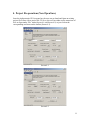
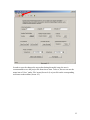
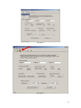
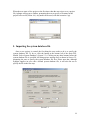
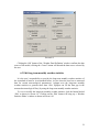
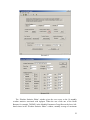
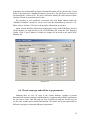
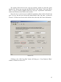
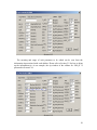
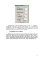
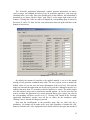
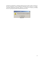
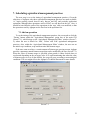
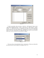
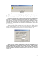
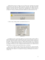
Agricultural Input Model
(AgInput)
User’s Manual
Documentation of Graphical User Interface
Prepared by Peng Wang and Arturo A. Keller
Bren School of Environmental Science & Management
University of California, Santa Barbara
www.bren.ucsb.edu
August 2004
1
Table of Contents
1.
INTRODUCTION ...........................................................................................4
2.
INSTALLING AGINPUT ................................................................................5
3.
PREPARING AGINPUT FILES .....................................................................6
3.1 System Database File ............................................................................................ 6
3.2 Meteorological data files....................................................................................... 8
3.3 Monthly weather statistics ................................................................................. 10
4.
PROJECT FILE OPERATIONS (NEW/OPEN/SAVE) .................................11
5.
IMPORTING THE SYSTEM DATABASE FILE ...........................................14
6.
IMPORTING WATERSHED AND CROP INFORMATION ..........................16
6.1 Input the watershed location data ..................................................................... 16
6.2 Weather Data Definition .................................................................................... 17
6.3 Edit long-term monthly weather statistics........................................................ 21
6.4 Choose crop type and edit the crop parameters .............................................. 23
6.5 Input the soil properties of the watershed ........................................................ 27
6.6 Input pesticides information .............................................................................. 28
7.
SCHEDULING AGRICULTURAL MANAGEMENT PRACTICES ...............33
7.1 Add an operation................................................................................................. 33
7.2 Edit an operation................................................................................................. 42
7.3 Delete an operation ............................................................................................. 43
8.
SET SIMULATION PERIOD........................................................................45
9.
RUN THE MODEL.......................................................................................47
2
10.
VIEW THE RESULTS ..............................................................................48
11.
REFERENCES: .......................................................................................50
12.
APPENDIX A ...........................................................................................51
3
1. Introduction
Agricultural Input Model (AgInput) is a model that simulates plant growth, developed
to predict the irrigation and nutrient (nitrogen and phosphorous) requirements of
agricultural crops, based on soil and meteorological conditions of a specific catchment or
watershed. AgInput can also help the user to simulate and manage pesticide application
operations. The plant growth component of AgInput is based on a simplified version of
the EPIC plant growth model (Neitsch et al. 2002). As discussed in AgInput’s technical
documentation, some modifications were made based on the objectives of AgInput.
AgInput is used to predict daily, monthly or annual application rate of fertilizer,
irrigation water, and pesticides, based on crop requirements, and considering local
conditions. The output is intended to be the input function for a variety of watershed
simulation models, or for evaluating crop management. The assumptions made in
AgInput (described in AgInput’s Technical Documentation) should be understood by the
user of AgInput.
The main Graphical User Interface (GUI) of AgInput is presented in Screen 1-1.
Screen 1-1
4
2. Installing AgInput
AgInput was coded using Microsoft Visual C++ 6.0 and, therefore, is compatible with
Windows 95/98/2000/Me/XP. Because AgInput is coded based on Microsoft MFC
(Microsoft Foundation Class) and the application is created using MFC in a shared DLL
(Dynamic Link Library) mode, the executable file named AgInput.exe is executable only
when four DLL files are present, which are MFC42D.DLL, MFCD42D.DLL,
MFCO42D.DLL and MSVCFTD.DLL. Therefore, in order to use AgInput, the user has
to have all of the above-mentioned files and they should all be in the same folder. The
folder name is a user’s decision.
In order to save the user’s time in preparing the necessary system database file, there
is a default system database file supplied with AgInput, named SystemDB.mdb, The
details of the file are discussed in Section 3-1. The user may change the name of the
system database file later as needed.
Basic files needed are:
AgInput.exe
MFC42D.DLL,
MFCD42D.DLL,
MFCO42D.DLL,
MSVCFTD.DLL,
SystemDB.mdb.
5
3. Preparing AgInput files
3.1 System Database File
For AgInput, information on crop and agricultural management practices are stored in
a file called the system database file (SystemDB.mdb). In most cases, the user will not
need to change the values of parameters in this file, although the user is given access to
the file within the AgInput GUI, in case the user has better information than the default
provided in the system database file. The system file that comes with AgInput was
prepared by using data directly from the SWAT (Neitsch et al. 2002) database.
For the system database file, AgInput can recognize only files in Microsoft Access
1997 or 2000 format, although the name of the file is a choice of the user. In case the user
wants to prepare a different system file, the Microsoft Access database file should have
three tables within it, whose names should be ‘crop’, ‘mgt’ and ‘pest’ respectively. The
user must not change the name of these three tables, otherwise AgInput will not run
properly. The structure of these three tables is presented in Table 3-1 through 3-3.
Table 3-1 Structure of ‘crop’ table
Field Name
ICNUM
CPNM
IDC
CROPNAME
BIO_E
HVSTI
BLAI
FRGRW1
LAgInputX1
FRGRW2
LAgInputX2
DLAI
CHTMX
RDMX
T_OPT
T_BASE
CNYLD
CPYLD
BN1
BN2
BN3
BP1
BP2
BP3
WSYF
USLE_C
Data Type
Integer
Text
Integer
Text
Double
Double
Double
Double
Double
Double
Double
Double
Double
Double
Double
Double
Double
Double
Double
Double
Double
Double
Double
Double
Double
Double
6
GSI
VPDFR
FRGMAX
WAVP
CO2HI
BIOEHI
RSDCO_PL
OV_N
CN2A
CN2B
CN2C
CN2D
FERTFIELD
Double
Double
Double
Double
Double
Double
Double
Double
Double
Double
Double
Double
Yes/No
Table 3-2 Structure of ‘mgt’ table
Field Name
OPNAME
CPNUM
Data Type
Text
Integer
Table 3-3 Structure of ‘pest’ table
Field Name
CROPNAME
PESTNAME1
PESTAMOUNT1
PESTSTD1
PESTNAME2
PESTAMOUNT2
PESTSTD2
PESTNAME3
PESTAMOUNT3
PESTSTD3
PESTNAME4
PESTAMOUNT4
PESTSTD4
PESTNAME5
PESTAMOUNT5
PESTSTD5
PESTNAME6
PESTAMOUNT6
PESTSTD6
PESTNAME7
PESTAMOUNT7
PESTSTD7
PESTNAME8
PESTAMOUNT8
PESTSTD8
PESTNAME9
Data Type
Text
Text
Double
Double
Text
Double
Double
Text
Double
Double
Text
Double
Double
Text
Double
Double
Text
Double
Double
Text
Double
Double
Text
Double
Double
Text
7
PESTAMOUNT9
PESTSTD9
PESTNAME10
PESTAMOUNT10
PESTSTD10
PESTNAME11
PESTAMOUNT11
PESTSTD11
PESTNAME12
PESTAMOUNT12
PESTSTD12
PESTNAME13
PESTAMOUNT13
PESTSTD13
PESTNAME14
PESTAMOUNT14
PESTSTD14
PESTNAME15
PESTAMOUNT15
PESTSTD15
PESTNAME16
PESTAMOUNT16
PESTSTD16
PESTNAME17
PESTAMOUNT17
PESTSTD17
PESTNAME18
PESTAMOUNT18
PESTSTD18
PESTNAME19
PESTAMOUNT19
PESTSTD19
PESTNAME20
PESTAMOUNT20
PESTSTD20
Double
Double
Text
Double
Double
Text
Double
Double
Text
Double
Double
Text
Double
Double
Text
Double
Double
Text
Double
Double
Text
Double
Double
Text
Double
Double
Text
Double
Double
Text
Double
Double
Text
Double
Double
The ‘pest’ table within the systemDB.mdb was prepared based on the crop’s pesticide
usage information at the state level of California. The AgInput Technical Documentation
describes the data source and processing to develop the ‘pest’ table. If the user has local
information, it is recommended that it be used instead.
3.2 Meteorological data files
AgInput requires daily values of precipitation, maximum and minimum temperature,
solar radiation, relative humidity and wind speed. The user may choose to read in these
inputs from files or generate the values using monthly average data summarized over a
8
number of years (see Section 3.3. for details on how to generate this data if not available
at the daily level).
AgInput requires the meteorological parameters to be organized as separate tables in a
single Microsoft Access Database file, whose name is a user’s choice. Within the
database file, the name of each table, if existing, should follow these requirements: ‘Pcp’
for daily precipitation, ‘Temp’ for daily maximum and minimum temperature, ‘Solar’ for
daily solar radiation, ‘Rh’ for daily relative humidity and ‘Wind’ for daily average wind
speed. If there is no data for a particular meteorological parameter, there is no need to
create a table within the database.
AgInput reads in the date only from the first record of the input meteorological file
and then calculates the date of a subsequent day according to the cumulative record count
before the day, so it is the user’s responsibility to make sure that there are no gaps in the
dates within each table. In the case where there is data gap for some day(s), the date
needs to be entered and the data field(s) should be filled in with –99.0 for these days.
AgInput uses –99.0 as a flag for missing measured data. In the case of missing data,
AgInput will use the weather generator to fill the data gap. The user needs to provide
appropriate monthly values for the weather generator.
Following are the structures of each table within the meteorological database file:
Table 3-4 Structure of ‘Pcp’ table
Field Name
DATE
PCP
Data Type
Date
Double
* The PCP field is in millimeter (mm) of precipitation, as water.
Table 3-5 Structure of ‘Temp’ table
Field Name
DATE
MAX
MIN
Data Type
Date
Double
Double
* Both MAX and MIN fields are in degrees Celsius.
Table 3-6 Structure of ‘Solar’ table
Field Name
DATE
SOLAR
Data Type
Date
Double
* The SOLAR field is in MJ/m2.
9
Table 3-7 Structure of ‘Rh’ table
Field Name
DATE
RH
Data Type
Date
Double
* The RH field is a fraction.
Table 3-8 Structure of ‘Wind’ table
Field Name
DATE
WIND
Data Type
Date
Double
* The WIND field is in m/s.
Alternatively, AgInput is also designed to be able to read in the meteorological data
files used for WARMF (Watershed Analysis Risk Management Framework). The file
name is a user’s choice. For the format of the WARMF meteorological data file, the user
can refer to the WARMF user’s manual (Herr et al., 2001)
3.3 Monthly weather statistics
If daily weather meteorological parameter values are not available AgInput can use
monthly weather statistics to generate daily values. The monthly weather statistics file
needs to be obtained or prepared by the user using long-term local historical weather
monitoring data of the watershed of interest. The file should be named ‘wgn.mdb’ and
should be in the same directory as the system database file. The file ‘wgn.mdb’ should
contain a table named exactly ‘wgn’, which stores all the necessary information. The user
can prepare these statistics from available meteorological data. Also, U.S. EPA’s
BASINS (Better Assessment Science Integrating point and Nonpoint Sources) provides
this data in the correct file format, either online or in a CD, for most Hydrologic
Cataloging Units (HCUs) in U.S. The structure of the file is presented in Appendix A.
10
4. Project file operations (New/Open/Save)
Once the AgInput main GUI is opened up, the user can go ahead and Open an existing
project file or start a New project file. To do so, the user can either use the menu item of
New or Open under ‘File’ menu (Screen 4-1 and Screen 4-2) or just click on the
corresponding tool items on the toolbar (Screen 4-3).
Screen 4-1
Screen 4-2
11
Screen 4-3
In order to save the changes the user makes during the model setup, the user is
recommended to save the project file from time to time. To do so, the user can use the
menu item of ‘Save’ under ‘File’ menu (Screen 4-4) or just click on the corresponding
tool items on the toolbar (Screen 4-5).
12
Screen 4-4
Screen 4-5
13
When the user starts a New project or the first time when the user tries to save a project
file, AgInput will pop up a window, prompting the user to specify a file name for the
project to be saved (Screen 4-6). Any name can be used, with the extension *.prj.
Screen 4-6
5. Importing the system database file
Once a new project is created, the first thing the user needs to do is to specify the
system database file. To do so, click the button at the bottom left of the main GUI,
labeled ‘Select System Database’ (Screen 5-1). Clicking on any other buttons before the
system database file is specified will bring open a message box as shown in Screen 5-2,
prompting the user to specify the system database file first. Please note that, although
AgInput supplies its user with a default system database file, it still asks the use to
specify the file in the first step.
Screen 5-1
14
Screen 5-2
Once the ‘Select System Database’ button is clicked, a dialog window will pop up
(Screen 5-3), which prompts the user to select a system database file.
Screen 5-3
In case the user selects an incorrect database file or the selected system database file
doesn’t include all the necessary tables, a message box will open (Screen 5-4), prompting
the user to reselect the correct database file.
Screen 5-4
15
6. Importing watershed and crop information
Once a system database file has been specified, the user can then input watershedspecific information, such as watershed location, the type of crop grown in the watershed,
soil data, and data sources for meteorological conditions.
6.1 Input the watershed location data
Accurate watershed location, including altitude, longitude and elevation, is important
for AgInput to generate reasonable solar radiation if measured solar radiation data is not
available. The user can input watershed location information within the main GUI of
AgInput as shown in Screen 6-1.
Screen 6-1
In order to keep AgInput from accepting unreasonable values, AgInput sets the range
for all of these parameters. The ranges of latitude and longitude, for example, are 0.0 to
60.0 for latitude and 0.0 to 180.0 for longitude. Both latitude and longitude are in radians.
16
Also, in order to provide the user with the information on each parameter which
requires an input value, an information tip presents the user with an explanation of each
parameter, and, in most cases, the range of the parameter values, if appropriate, is added
to each editbox in AgInput. The information tip will be brought up whenever the user
scrolls the mouse across the editbox, and the tip window will last for 5 seconds. The tip
window of the editbox of latitude is presented as an example in Screen 6-2.
Screen 6-2
6.2 Weather Data Definition
As mentioned before, AgInput can predict nutrient and water needs of each crop type
based on the local meteorological conditions. In AgInput, the local meteorological
conditions are provided either as measured daily meteorological data or as generated
meteorological data based on long-term monthly weather statistics. Although AgInput
can generate meteorological data based on long-term monthly weather statistics of the
watershed of interest when the measured data is unavailable, the user is strongly
recommended to provide the measured meteorological information because it will
significantly increase the accuracy of model results.
To define whether the meteorological conditions are from the measured data or from
generated data, the user needs to click the ‘Define’ button within the ‘Weather Data
Definition’ group box (Screen 6-3), which will bring up the ‘Weather Data Definition’
17
window (Screen 6-4), where the user can define the data source for each meteorological
parameter, i.e. precipitation, temperature, solar radiation, relative humidity and wind
speed.
Screen 6-3
Screen 6-4
18
The data source of each meteorological parameter can be simulated data or measured
data. By default, AgInput sets the data source of each meteorological parameter to be
‘simulated’ (Screen 6-4). To import the measured data of one of the five parameters into
the model, the user needs to click the Radio Button labeled as ‘Measured’ under the
group box corresponding to the parameter.
Taking precipitation as an example, when the ‘Measured’ radio button is clicked, the
button, labeled as ‘Where’ to its right, is activated. When the ‘Where’ button is clicked, a
‘Rain Data Location’ window is brought up (Screen 6-5).
Screen 6-10
The ‘Rain Data Location’ window can direct the user to select the measured
precipitation file either in the format of Microsoft Access Database (Screen 6-5) or in the
format of WARMF meteorological database (Screen 6-6). The user can switch between
two file formats by clicking on the edit box to the right of the text ‘Files of type’ (Screen
6-7).
19
Screen 6-6
Screen 6-7
Once the user selects an appropriate precipitation file and clicks the ‘Open’ button of
the ‘Rain Data Location’ window, the ‘Rain Data Location’ window will close and the
edit box to the right of the text of ‘Location’ within the group box of ‘Precipitation Data’
of the ‘Weather Data Definition’ will show the file name and the full path of the selected
precipitation file (Screen 6-8).
20
Screen 6-8
Clicking the ‘OK’ button of the ‘Weather Data Definition’ window confirms the data
source of the model; clicking the ‘Cancel’ button will discard the data source selected by
the user.
6.3 Edit long-term monthly weather statistics
It is the user’s responsibility to provide the long-term monthly weather statistics of
the watershed of interest. As mentioned before, in case where the user has no measured
data for certain meteorological parameter(s), AgInput uses the long-term monthly
weather statistics to generate these data. Also, AgInput can fill the data gap in the
measured meteorological file(s) by using the long-term monthly weather statistics.
To view or modify the long-term monthly weather statistics, click the button labeled
‘Edit’ as shown in Screen 6-9. Clicking on the ‘Edit’ button will bring up a ‘Weather
Statistics Editor’ window as shown in Screen 6-10.
21
Screen 6-9
Screen 6-10
The ‘Weather Statistics Editor’ window gives the user access to the 14 monthly
weather statistics associated with AgInput. When the user clicks one of the Radio
Buttons, for example, TMPMX, in the Monthly Parameters Group Box on the lower lefthand corner in the ‘Weather Statistics Editor’ window, monthly average of maximum
22
temperature for each month from January through December will be shown in the 12 edit
boxes to the right of the ‘Monthly Parameters’ group box. The edit boxes are labeled as
Jan. through Dec. (Screen 6-10). The user is allowed to modify the values shown in these
edit boxes, based on watershed specific data.
The meaning of each parameter associated with each Radio Button within the
‘Monthly Parameters’ group box can be seen from the information tip (Screen 6-11).
Please refer to Section 5-2 for how to bring up the information tip window.
Again, caution should be taken when modifying the values in the Edit Boxes, because
all the changes are made directly to the WGN database file when the ‘OK’ Button is
clicked. If the ‘Cancel’ Button is clicked, no change will be made to the initial WGN
database file.
Screen 6-11
6.4 Choose crop type and edit the crop parameters
Although there are over 90 crops in the current database, AgInput at present
determines the nutrient (nitrogen and phosphorus), irrigation and pesticide requirements
for one crop at a time. Note that only one crop is modeled in each run, but the user can
use the same weather and watershed information. The model can be run sequentially for
different crop types to obtain the different requirements.
23
The user needs to select a crop type for the analysis. To do so, the user needs to click
on the button on the main GUI, labeled ‘Select Crop Type’ (Screen 6-12), which brings
up the ‘crop type selection’ window. This window presents all the crop types in a list box
(Screen 6-13).
Screen 6-12
Screen 6-13
24
The content of the list box in the ‘crop type selection’ window are from the system
database file. Choose one crop type and then click the ‘OK’ button. If the user fails to
select a crop, by default AgInput selects the crop type ‘Agricultural Land-Generic’,
which is the first one in the list box in the window.
Next, the user is given access to modify the parameter values of the selected crop
type. To do so, the user can click on the button labeled ‘Edit Crop Data’, as shown in
Screen 6-14. Most users do not need to edit the data, unless they have better information.
Screen 6-14
Clicking on the ‘Edit Crop Data’ button will bring up a ‘Crop Parameter Editor’
window, as shown in Screen 6-15.
25
Screen 6-15
The meaning and range of each parameter to be edited can be seen from the
information tip associated with each editbox. Please refer to Section 5-2 for how to bring
up the information tip. As an example, the tip window of the editbox for ‘BIO_E’ is
presented in Screen 6-16.
Screen 6-16
26
Caution should be taken when the user is modifying the parameters of the crop
selected, because, once the ‘OK’ button in the ‘Crop Parameter Editor’ is clicked, all the
changes the user are made directly in the system database file. If the ‘Cancel’ button is
clicked, no change is made to the database file.
6.5 Input the soil properties of the watershed
Certain soil properties are taken into consideration when AgInput estimates the
nutrient and water needs of a crop. To set the values of these soil properties, the user
needs to click the ‘Edit’ button within the ‘Soil Data’ group box of the main GUI (Screen
6-17), which brings up the ‘Soil Data Editor’ window (Screen 6-18), allowing the user to
modify the values of the soil properties.
Screen 6-17
27
Screen 6-18
The default value of each soil parameter is shown in Screen 6-18. To keep the
changes made to these values, click ‘OK’ button, otherwise, click ‘Cancel’ button to
discard all the changes. Also, an information tip is available for each edit box in the ‘Soil
Data Editor’ window. Note that although maximal canopy storage is not strictly a soil
parameter, it is relevant to the calculation of soil evaporation.
6.6 Input pesticides information
AgInput provides the user with a ‘pest’ table within the System database file, which
was prepared using the pesticides usage information at the state level in California from
1998 to 2002. The user can also set the amount of pesticides to be applied. Within the
main GUI of AgInput, clicking the button labeled ‘Select Pesticide’ will give the user
access to the information contained in the ‘pest’ table (Screen 6-19). Clicking the ‘Select
Pesticide’ button will bring up the ‘Pesticide crop type’ window shown in Screen 6-20.
28
Screen 6-19
Since the ‘pest’ table in the system database file was prepared using Summaries of
Pesticide Use Report Data of 1998 to 2002 (DPR CA, 2003), the crop types in the ‘pest’
table does not exactly match those in ‘crop’ table within the same file, which was from
the SWAT database. The advantage of treating pesticides data this way is that in case
SWAT crop database is updated later, the changes will not affect AgInput’s pesticides
database, i.e., the data stored in ‘pest’ table. This independence of the databases requires
the user to explicitly specify the type of crop in each section.
29
Screen 6-20
Clicking the ‘OK’ button in the ‘Pesticide crop type’ button will bring up the ‘Pesticide
application information’ windows as shown in Screen 6-21, while clicking ‘Cancel’ will
discard the selection.
Screen 6-21
30
The ‘Pesticides application information’ window presents information on names,
yearly average, and standard deviation of top 20 pesticides applied to each crop type
contained in the ‘pest’ table. Due to the limited space in the windows, the information is
presented in two pages, labeled ‘Page1’ and ‘Page2’ on the upper right corner of the
window. Clicking one of the two tabs will display the corresponding page as shown in
Screens 6-21 and 6-22. Note also the conversion factor between kg/ha and lb/ac at the
bottom of each screen.
Screen 6-22
By default, the amount of pesticides to be applied annually is set to be the annual
average of each pesticide contained in the table. The user is given access to modify the
default values, in case the user has better information at the local level. Note that the
model can calculate the application rate for all top 20 pesticides, although in practice it is
unlikely that more than 2-3 pesticides would be applied in a season. The model simply
uses the statistical usage rate to calculate the amount applied. In case the user does not
want to calculate the application of a certain pesticide shown in two pages, the value in
the corresponding edit boxes can be set to 0. Clicking ‘OK’ button in the ‘Pesticide
application information’ window saves all the set values for the simulation, while
clicking ‘Cancel’ discards all changes just made.
Note that the modifications to the pesticides usage data are valid only for a
simulation. No change will be made to the ‘pest’ table regardless of whether the ‘OK’
button is clicked or not. Also, AgInput has no a default value for the types and amount of
31
pesticides to be applied for a simulation, therefore, the user needs to make sure that he or
she has specified the pesticide application information before moving on to arrange
agricultural management operations. Otherwise, a message box will pop up, prompting
the user to specify the pesticides information first (Screen-23).
Screen 6-23
32
7. Scheduling agricultural management practices
The next step is to set the timing of agricultural management practices. Given the
objectives of AgInput, only three agricultural management practices are made available,
i.e., begin growing season, harvest only, harvest and kill, and pesticide application
operations, although other operations used in SWAT are still shown in the list. Also, it
should be noted that the order of the operations in the ‘mgt’ table was modified, so that
the operations used by AgInput are the first four in the operations list.
7.1 Add an operation
To set the timing of the agricultural management practices, the user needs to click the
‘Timing’ button within the ‘Agricultural Management’ group box of the main GUI
(Screen 7-1), which brings up the ‘Agricultural Management Editor’ window (Screen 72), where the user is allowed to ‘Add’, ‘Delete’ and ‘Edit’ agricultural management
practices. Also, within the ‘Agricultural Management Editor’ window, the user can set
the initial crop conditions, crop total heat units and biomass target.
If the user wants to achieve a certain amount of biomass per growing season, AgInput
provides a parameter named biomass target that can be modified by the user (Screen 7-2).
When the value of biomass target is specified, plant growth is either slowed down or
accelerated depending on the set target value. It is worth mentioning that when the value
of biomass target is set to 0 (the default), the crop will grow according to meteorological
conditions. The user might refer to the AgInput’s Technical Document for more details.
Screen 7-1
33
Screen 7-2
To add an operation, the user needs to click the ‘Add Operation’ button in the
‘Agricultural Management Editor’ window, which opens an ‘Add Operation’ window
(Screen 7-3), within which there is a dropdown list, which lists all the agricultural
operations present in the system database file. Although there are a total of 12 operations
shown in the list, only the top four (begin growing season, harvest only, pesticide
application, and harvest and kill) are operational in AgInput.
Screen 7-3
If the user selects a non-operational activity, a message box will pop up, warning that
the operation hasn’t been incorporated in AgInput (Screen 7-4).
34
Screen 7-4
AgInput allows the user to arrange up to three growing seasons per year. Each
growing season must start with a ‘Begin growing season’ operation. Therefore, the user
should always start a growing cycle by choosing a ‘Begin growing season’ operation
from the operation list.
Clicking the ‘OK’ button after the ‘Begin growing season’ operation has been chosen
in Screen 7-3 will bring up a ‘Plant/begin growing season’ editor window (Screen 7-5),
which shows the name of the crop selected to be grown, the operation name, and also
allows the user to specify the order of the growing season in a year cycle, i.e., first,
second and third, the starting date of the operation and the initial heat unit fraction when
the operation starts.
AgInput schedules all the operations based on heat units, except ‘Begin growing
season’, which is scheduled by date. This is done so that AgInput can easily locate the
starting record within the meteorological files, as all of them are ordered by date.
Screen 7-5
For any of the four operations, AgInput requires a value to be specified for ‘Order of
growing season’ and there is not default value in AgInput. Therefore, for any agricultural
operation, clicking ‘OK’ button before a value for ‘Order of growing season’ has been
specified will bring up a message box, prompting the user to select a growing season first
(Screen 7-6).
35
Screen 7-6
The user cannot skip any previous growing season(s) before he or she can schedule the
next one. In other words, the user should always start with the first growing season, then
the second if appropriate, and finally the third if appropriate. Otherwise, either Screen 7-7
or Screen 7-8 will pop up.
Screen 7-7
Screen 7-8
After a ‘Begin growing season’ has been scheduled for a growing season, the user can
then go ahead and schedule three other operations for the growing season, which are
optional. Choosing ‘Harvest only’ or ‘Harvest and kill’, before a ‘Begin growing season’
operation has been scheduled will bring up a message box, prompting the user to first
schedule a ‘Begin growing season’ (Screen 7-9).
Screen 7-9
36
AgInput allows the user to arrange up to two ‘Harvest only’ operations per growing
season, but no more than one ‘Harvest and kill’ operation. The ‘Harvest and kill’
operation, if selected, must be the last operation of a growing season. Whenever the user
attempts to put more than two ‘Harvest only’ operations into a growing season, a
message box will pop up, indicating that further addition is not allowed (Screen 7-10).
Screen 7-10
A ‘Harvest only’ editing window is presented in Screen 7-11.
Screen 7-11
In AgInput, the user is given the option to set a harvest index override, which is
different from the harvest index calculated by the model. If a harvest index override is set
by the user, the harvest index override is used in place of the harvest index calculated by
the model. If the user leaves the value of ‘Harvest Index Override’ as 0, as shown in
Screen 7-11, AgInput will assume that the user wants to use the harvest index calculated
by AgInput. The user may refer to AgInput technical document to see what the harvest
index and harvest index override mean and how they are calculated.
The user is not allowed to add a ‘Harvest only’ operation after a ‘Harvest and kill’
operation or add a ‘Harvest and kill’ operation before any other operations in terms of
fraction heat units. Otherwise, a message box will pop up, indicating an error (Screen 712 and 7-13).
37
Screen 7-12
Screen 7-13
A ‘Harvest and kill’ editing window is presented in Screen 7-14.
Screen 7-14
The heat unit fraction of ‘Harvest only’ operation should be somewhere between 0.4
and 1.25 and the heat unit fraction of ‘Harvest and kill’ operation should be no less than
0.7 and no more than 1.25. If the heat unit fraction values are outside these ranges, the
input values will not be accepted and a message box will pop up, prompting the user to
re-enter an appropriate value instead. Screen 7-15 is given as an example.
Screen 7-15
38
AgInput requires that the time span of two adjacent growing seasons be no less than
60 days and the time span between the date when the first growing season starts and that
when the third growing season starts cannot exceed 300 days, so that the three crops are
harvested within one year. Warning messages are provided by the model (Screens 7-16
and 7-17).
Screen 7-16
Screen 7-17
A ‘Pesticide application’ operation can be scheduled at any anytime point before the
‘Harvest and kill’ operation of a growing season. A ‘Pesticide application’ operation
window is presented in Screen 7-18.
Screen 7-18
Note that pesticide may be applied before the first growing season. However, to be
reasonable, AgInput allows the user to set no more than one ‘Pesticide application’
operation before the ‘Begin growing season’ operation of a growing season. When the
39
user attempts to put more than one ‘Pesticide application’ operation before a ‘Begin
growing season’, a message box will pop up (Screen 7-19)
Screen 7-19
Also, AgInput does not set a limit to the number of ‘Pesticide application’ operations
within a growing season. The user can consider as many ‘Pesticide application’
operations as needed.
For the user’s convenience, AgInput was designed to allow the user to add operations
other than ‘Begin growing season’ anytime as long as the order of the growing season is
specified and reasonable heat units are provided. In other words, the user does not have to
finish arranging all the operations for the first (or second) growing season before he or
she can schedule operations for the next growing season(s). The user can always add
operations later as needed as long as the growing season order is specified and the heat
units are reasonable.
When an operation is successfully added, it will appear in the list box on the lower
left-hand corner of the ‘Agricultural Management Editor’ window, with growing season
shown in a column labeled ‘Season’, operation name in a column labeled ‘Operations’
and heat units fraction in a column labeled ‘Heat Units’. Screen 7-20 is given as an
example of a complete schedule of agricultural operations. Note that many crops can only
be grown once or twice per year. Please note, for the user to see all the three growing
seasons in this example, no pesticide application operations were incorporated into the
list.
40
Screen 7-20
The agricultural management operations listed in Screen 7-20 were arranged for a
one-year cycle from Jan. 1, 1990 to Dec. 31, 1990 and the same pattern will be repeated
every succeeding year in the entire simulation period. The agricultural management
operation list as shown in Screen 7-20 was simulated for the crop ‘Agricultural LandGeneric’, using meteorological data from the Napa River Watershed in California. The
simulated biomass dynamics for the first year, i.e., Jan. 1 1990 to Dec. 31, 1990, is
presented in Figure 7-1.
41
As mentioned earlier, to arrange a ‘Begin growing season’, the user must specify the
date at which the growing season starts. For the simulation, the first growing season starts
at Jan. 1 each year, the second growing season starts at Jun. 1 each year, and the third
growing season starts at Aug. 20.
There are 3 full growing seasons within the year, bounded by the red lines. In Figure
7-1, the simulated plant biomass is presented in y axis along with date, which is in x axis.
Fraction heat units (FHU) is marked at each time point where an agricultural operation
occurs. The first growing season started on Jan. 1, 1990 and ended May 31, 1990, lasting
5 months, but as one can see, the fraction heat units for the second ‘Harvest only’
operation was not reached, which is 0.8. Therefore, the ‘Harvest only’ and the succeeding
‘Harvest and kill’ operation arranged for the first growing season were not got executed.
The reason for this is the fraction heat units did not accumulate fast enough for the plant
to reach the maturity during the first growing season because of the relatively low
temperature in these months. This serves to remind the user of the importance of
considering local meteorological conditions and crop specific parameters when arranging
agricultural operations for a specific catchment or a watershed.
For the second and third growing seasons, all the operations were completed. It
should be pointed out that the fraction heat units for the ‘Harvest and kill’ operation of
the second growing season was set to be 1.25 and this is the reason why the simulated
biomass stays constant from FHU=1.0 to FHU=1.25. The user can refer to the AgInput’s
technical manual to see how each operation functions.
7.2 Edit an operation
To modify any operation already scheduled, choose the operation to be modified and
then click the ‘Edit Operation’ button or just simply double-click the operation to be
modified, either of which will bring up an editor window for the operation selected.
AgInput allows the user to modify all the parameters of the operation except growing
seasons and starting date of the growing seasons. Following are examples of a ‘Begin
growing season’ and a ‘Harvest only’ editor window (Screen 7-21 and 7-22). For
parameters that are no longer editable, the corresponding edit boxes appear gray.
Screen 7-21
42
Screen 7-22
When modifying the value of parameters, especially fraction heat units, the user
should be careful to make sure that the rules mentioned in Section 7.1 are not violated.
Otherwise, message boxes will pop up, indicating the errors.
7.3 Delete an operation
The user can delete an operation scheduled earlier. In order to delete an operation,
first select the operation to be deleted in the scheduled operation list on the lower lefthand side of the ‘Agricultural Management Editor’ window, and then click the ‘Delete
Operation’ button to the right of the scheduled operation list.
Clicking the ‘Delete Operation’ button before any scheduled operation has been
selected will bring up a message box (Screen 7-23), prompting the user to make a
selection first.
Screen 7-23
A ‘begin growing season’ operation can only be deleted when it is the only operation
left in the growing season. Thus, in order to remove a growing season entirely, the user
should start deleting the other operations of the growing season before deleting the ‘begin
growing season’ operation. If the user attempts to delete a ‘begin growing season’
operation that is not the last operation left in the growing season, a message box will pop
up, telling the user that the operation cannot be deleted (Screen 7-24). Also, when the
user is trying to delete a growing season entirely when a later growing season is present,
43
the same message box as shown in Screen 7-17 will pop up, telling the user that the
operation cannot be deleted.
Screen 7-24
44
8. Set simulation period
The final step is to set the simulation period. When there is at least one measured
daily meteorological data file defined for the simulation, as discussed in Section 5-4, the
possible range of simulation dates is automatically set according to the date range of the
data in these files. When the user is scheduling agricultural operation as discussed in
Section 6, the simulation starting point is also changed accordingly to the starting point of
the first growing season scheduled. After all the meteorological data sources have been
defined and all the agricultural operations have been scheduled, the user can still change
the simulation period by manually change the starting and ending point in the main GUI
of AgInput (Screen 8-1), within the available range of dates. Although the user can
reduce the range of dates, it is recommended to always use full years to produce
meaningful output.
When there are no daily meteorological files defined for the simulation, the
simulation range can be from the starting point of the first growing season scheduled to
any time point forward as long as the simulation span is more than 180 days. It is
recommended to use at least a full year.
Screen 8-1
45
Within the possible range of simulation dates, the user can set the simulation starting
and ending point as long as the starting point is no later than ending point. Otherwise, a
message box will pop up, warning the user of the error (Screen 8-2).
Screen 8-2
When the simulation duration is set to be less than 180 days, a message box will pop
up, indicating the error (Screen 8-3).
Screen 8-3
46
9. Run the model
Now, you are ready to run the model. When everything is ready, clicking the ‘Run
Source Model’ will start the run.
Since AgInput does not have default settings for the agricultural operations, AgInput
checks the scheduled agricultural operations before it runs the model just in case the user
might have forgotten to schedule agricultural operations before clicking the ‘Run Source
Model’ button. When this happens, a message box will pop up (Screen 9-1), prompting
the user to schedule agricultural management operations first.
Screen 9-1
47
10.
View the results
Once a run of AgInput has been successfully completed, two Microsoft Access
database files named ResultDB.mdb and PestDB.mdb are created under the same
directory as the executable file of AgInput.exe. Both database files contain 2 separate
tables within them, with ‘DailyOuput’ and ‘MonthlyOuput’ in ResultDB.mdb and
‘DailyPest’ and ‘MonthlyPest’ in PestDB.mdb.
The table ‘DailyOutput’ contains fields for simulation date, reproduced or generated
meteorological data, simulated daily irrigation water requirements, and daily nitrogen and
phosphorus needs. The table ‘MonthlyOuput’ contains fields for monthly averages of the
irrigation water, nitrogen and phosphorus needs over the simulation periods.
The structure of the DailyOutput and ‘MonthlyOutput’ tables is presented in Table
10-1 and Table 10-2.
Table 10-1 Structure of ‘DailyOutput’ table
Field Name
SimuDate
Precipitation
Min_Temp
Max_Temp
Solar_Radiation
RelativeHumidity
WindSpeed
Water_Need
N_Need
P_Need
Data Type
Date
Double
Double
Double
Double
Double
Double
Double
Double
Double
Unit
Mm/dd/yyyy
Mm
o
C
o
C
MJ/m2
Fraction
m/s
mm/day
kg N/day
kg P/day
Table 10-2 Structure of ‘MonthlyOutput’ table
Field Name
Month
Water_Need
N_Need
P_Need
Data Type
Integer
Double
Double
Double
Unit
mm/month
kg N/month
kg P/month
The table ‘DailyPest’ contains fields for simulation date, and daily amount (kg) of
pesticides applied per hectare and the table ‘MonthlyPest’ contains fields for month and
monthly average pesticide application to the crop averaged over the entire simulation
period. Both tables contain application amount for the top 20 pesticides used for this
crop. Since the pesticides vary from crop to crop, instead of using pesticide name, the two
tables display the pesticide number, arranged according to the editing screens (Screens 621 and 6-22). The structure of the ‘DailyPest’ and ‘Monthlypest’ tables is presented in
Tables 10-3 and 10-4.
48
Table 10-3 Structure of ‘DailyPest’ table
Field name
SimuDate
PEST1
PEST2
PEST3
PEST4
PEST5
PEST6
PEST7
PEST8
PEST9
PEST10
PEST11
PEST12
PEST13
PEST14
PEST15
PEST16
PEST17
PEST18
PEST19
PEST20
Data type
Date
Double
Double
Double
Double
Double
Double
Double
Double
Double
Double
Double
Double
Double
Double
Double
Double
Double
Double
Double
Double
*Note all fields except SimuDate are in kg ha-1day-1.
Table 10-4 Structure of ‘MonthlyPest’ table
Field name
Month
PEST1
PEST2
PEST3
PEST4
PEST5
PEST6
PEST7
PEST8
PEST9
PEST10
PEST11
PEST12
PEST13
PEST14
PEST15
PEST16
PEST17
PEST18
PEST19
PEST20
Data type
Integer
Double
Double
Double
Double
Double
Double
Double
Double
Double
Double
Double
Double
Double
Double
Double
Double
Double
Double
Double
Double
*Note all fields except Month are in kg ha-1month-1.
49
11. References:
1. Herr, J., L. Weintraub, C. W. Chen, User’s Guide to WARMF: Documentation of
Graphical User Interface, Final Report, 2001.
2. Neitsch, S.L., Arnold, J.G., Kiniry, J.R., Williams, J.R., Soil and Water
Assessment Tool User’s Manual, Version 2000, 2002.
50
12. Appendix A
Structure of ‘wgn’ table
SUBBASIN
STATION
WLATITUDE
WLONGITUDE
WELEV
RAIN_YRS
TMPMX1
TMPMX2
TMPMX3
TMPMX4
TMPMX5
TMPMX6
TMPMX7
TMPMX8
TMPMX9
TMPMX10
TMPMX11
TMPMX12
TMPMN1
TMPMN2
TMPMN3
TMPMN4
TMPMN5
TMPMN6
TMPMN7
TMPMN8
TMPMN9
TMPMN10
TMPMN11
TMPMN12
TMPSTDMX1
TMPSTDMX2
TMPSTDMX3
TMPSTDMX4
TMPSTDMX5
TMPSTDMX6
TMPSTDMX7
TMPSTDMX8
TMPSTDMX9
TMPSTDMX10
TMPSTDMX11
TMPSTDMX12
TMPSTDMN1
Integer
Text
Double
Double
Double
Integer
Double
Double
Double
Double
Double
Double
Double
Double
Double
Double
Double
Double
Double
Double
Double
Double
Double
Double
Double
Double
Double
Double
Double
Double
Double
Double
Double
Double
Double
Double
Double
Double
Double
Double
Double
Double
Double
51
TMPSTDMN2
TMPSTDMN3
TMPSTDMN4
TMPSTDMN5
TMPSTDMN6
TMPSTDMN7
TMPSTDMN8
TMPSTDMN9
TMPSTDMN10
TMPSTDMN11
TMPSTDMN12
PCPMM1
PCPMM2
PCPMM3
PCPMM4
PCPMM5
PCPMM6
PCPMM7
PCPMM8
PCPMM9
PCPMM10
PCPMM11
PCPMM12
PCPSTD1
PCPSTD2
PCPSTD3
PCPSTD4
PCPSTD5
PCPSTD6
PCPSTD7
PCPSTD8
PCPSTD9
PCPSTD10
PCPSTD11
PCPSTD12
PCPSKW1
PCPSKW2
PCPSKW3
PCPSKW4
PCPSKW5
PCPSKW6
PCPSKW7
PCPSKW8
PCPSKW9
PCPSKW10
PCPSKW11
PCPSKW12
PR_W1_1
Double
Double
Double
Double
Double
Double
Double
Double
Double
Double
Double
Double
Double
Double
Double
Double
Double
Double
Double
Double
Double
Double
Double
Double
Double
Double
Double
Double
Double
Double
Double
Double
Double
Double
Double
Double
Double
Double
Double
Double
Double
Double
Double
Double
Double
Double
Double
Double
52
PR_W1_2
PR_W1_3
PR_W1_4
PR_W1_5
PR_W1_6
PR_W1_7
PR_W1_8
PR_W1_9
PR_W1_10
PR_W1_11
PR_W1_12
PR_W2_1
PR_W2_2
PR_W2_3
PR_W2_4
PR_W2_5
PR_W2_6
PR_W2_7
PR_W2_8
PR_W2_9
PR_W2_10
PR_W2_11
PR_W2_12
PCPD1
PCPD2
PCPD3
PCPD4
PCPD5
PCPD6
PCPD7
PCPD8
PCPD9
PCPD10
PCPD11
PCPD12
RAINHHMX1
RAINHHMX2
RAINHHMX3
RAINHHMX4
RAINHHMX5
RAINHHMX6
RAINHHMX7
RAINHHMX8
RAINHHMX9
RAINHHMX10
RAINHHMX11
RAINHHMX12
SOLARAV1
Double
Double
Double
Double
Double
Double
Double
Double
Double
Double
Double
Double
Double
Double
Double
Double
Double
Double
Double
Double
Double
Double
Double
Double
Double
Double
Double
Double
Double
Double
Double
Double
Double
Double
Double
Double
Double
Double
Double
Double
Double
Double
Double
Double
Double
Double
Double
Double
53
SOLARAV2
SOLARAV3
SOLARAV4
SOLARAV5
SOLARAV6
SOLARAV7
SOLARAV8
SOLARAV9
SOLARAV10
SOLARAV11
SOLARAV12
DEWPT1
DEWPT2
DEWPT3
DEWPT4
DEWPT5
DEWPT6
DEWPT7
DEWPT8
DEWPT9
DEWPT10
DEWPT11
DEWPT12
WNDAV1
WNDAV2
WNDAV3
WNDAV4
WNDAV5
WNDAV6
WNDAV7
WNDAV8
WNDAV9
WNDAV10
WNDAV11
WNDAV12
Double
Double
Double
Double
Double
Double
Double
Double
Double
Double
Double
Double
Double
Double
Double
Double
Double
Double
Double
Double
Double
Double
Double
Double
Double
Double
Double
Double
Double
Double
Double
Double
Double
Double
Double
54