Download Software Package on Integrated Nonlinear Dynamic Modeling and

AFRL-RZ-WP-TR-2011-2005
SOFTWARE PACKAGE ON INTEGRATED NONLINEAR
DYNAMIC MODELING AND FIELD ORIENTED
CONTROL (FOC) OF PERMANENT MAGNET (PM)
MOTOR FOR HIGH PERFORMANCE
ELECTROMECHANICAL ACTUATORS (EMAs)
Quinn Leland
Mechanical Energy Conversion Branch
Power Division
Thomas X. Wu, Louis Chow, David Woodburn, Lei Zhou, Jared Bindl, Yang Hu, and Wendell Brokaw
University of Central Florida
JANUARY 2011
Interim Report
Approved for public release; distribution unlimited.
See additional restrictions described on inside pages
STINFO COPY
AIR FORCE RESEARCH LABORATORY
PROPULSION DIRECTORATE
WRIGHT-PATTERSON AIR FORCE BASE, OH 45433-7251
AIR FORCE MATERIEL COMMAND
UNITED STATES AIR FORCE
NOTICE AND SIGNATURE PAGE
Using Government drawings, specifications, or other data included in this document for any
purpose other than Government procurement does not in any way obligate the U.S.
Government. The fact that the Government formulated or supplied the drawings, specifications,
or other data does not license the holder or any other person or corporation; or convey any
rights or permission to manufacture, use, or sell any patented invention that may relate to them.
This report was cleared for public release by the USAF 88th Air Base Wing (88 ABW) Public
Affairs Office (PAO) and is available to the general public, including foreign nationals. Copies
may be obtained from the Defense Technical Information Center (DTIC) (http://www.dtic.mil).
AFRL-RZ-WP-TR-2011-2005 HAS BEEN REVIEWED AND IS APPROVED FOR
PUBLICATION IN ACCORDANCE WITH THE ASSIGNED DISTRIBUTION STATEMENT.
*//signature//
_______________________________________
//signature//
______________________________________
QUINN LELAND
Engineer
Mechanical Energy Conversion Branch
JACK VONDRELL
Chief
Mechanical Energy Conversion Branch
This report is published in the interest of scientific and technical information exchange and its
publication does not constitute the Government’s approval or disapproval of its ideas or
findings.
*Disseminated copies will show “//signature//” stamped or typed above the signature blocks.
Table of Contents Part I - Technical Manual .............................................................................................................. .1
I.
Introduction ............................................................................................................................. 1
II. Simulation Flow Chart ............................................................................................................ 3
III. Electrical Model ...................................................................................................................... 4
1.
Dynamical Equations ....................................................................................................... 4
2.
Time Stepping .................................................................................................................. 6
3.
Field Oriented Control (FOC) .......................................................................................... 7
IV. Thermal Model ........................................................................................................................ 9
1.
Model Setup ..................................................................................................................... 9
2.
Dynamic Thermal Equations ......................................................................................... 12
V. References ............................................................................................................................. 13
Part II - User’s Manual ................................................................................................................. 15
I.
Introduction ........................................................................................................................... 15
a.
Purpose of the Software .................................................................................................. 15
b.
Software Capability ........................................................................................................ 15
c.
User Privileges ................................................................................................................ 15
II. Input Parameters .................................................................................................................... 16
III. Software Startup .................................................................................................................... 20
IV. Software Execution and Procedure........................................................................................ 20
V. Output Parameters ................................................................................................................. 21
VI. Expected Results.................................................................................................................... 22
iii
Part III - Source Code (foc.m) ...................................................................................................... 33
Part IV - Motor Parameter Code (motorparameters.m) ................................................................ 44
iv
Part I ‐ Technical Manual I.)
Introduction
The development of all-electric aircraft is a high priority in the avionics community. Current
aircraft use a combination of hydraulic, pneumatic, and electric systems for flight control.
However, the expectation for future airplanes is a single, electric system using electromechanical
actuators (EMAs). Such a system would reduce the cost to build, operate, and maintain aircraft.
It would also make aircraft lighter, more reliable, safer, and more easily reconfigurable, reducing
the turnaround for new technology.
One of the greatest hurdles to replacing all hydraulic actuators with EMAs is heat generation, a
consequence of the absence of cooling hydraulic fluid. Accurately quantifying the heat
generated is complicated by the highly transient and localized nature of the power demands of an
EMA's motor, an especially significant issue in aircraft. Thus, accurate modeling must be
dynamic.
The parameters that characterize the motor are nonlinear functions. In steady-state analysis,
these nonlinearities can simply be averaged out, and often the parameters are considered to be
constant [1]. But during transient analysis these nonlinearities can become critical [2].
Consequently, time-averaged, linear models [3] are inadequate for thermal analysis and
management designs. So, proper treatment of the problem requires dynamic, nonlinear analysis.
The motor parameters can be determined by careful experimentation [2-3], but this is a time
intensive process and can be expensive especially when considering multiple potential designs
for a motor. Jens Otto suggested using a reduced order coenergy model [4], which yielded
results comparable to FEM results. Likewise, Roshen considered more involved empirical
formulas which accounted for excess eddy current losses [5].
Through FEM modeling, the nonlinear parameters, such as self and mutual inductances of the
three phase windings, can be determined [6-7]. Though dynamic FEM can be very accurate [4],
such detailed simulation is very slow. Fortunately, FEM is only necessary to quantify the
parameters; it is not necessary for simulating the motor over lengthy mission profiles. Instead, a
nonlinear, lumped element model (NL-LEM) can use the parameters from the FEM model and
then dynamically simulate the motor just as accurately as the FEM model but at a much lower
computational cost. To our knowledge, we are the first to address the nonlinear dynamic
modeling of a permanent magnet motor and describe both the control and thermal performance
of the motor in following highly transient mission profiles.
1
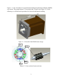
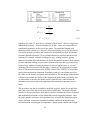
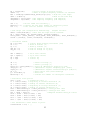
Figure 1.1 is the 3-D model of a typical Permanent Magnet Synchronous Machine (PMSM)
servo motor. This design features a 12-slot stator and a 10-pole rotor (Figure 1.2). In the
following, we will discuss the procedures for electrical and thermal modeling.
Figure 1.1. 3-D model of the PMSM motor design.
Figure 1.2. Cross-section of motor and rotor.
2
II.)
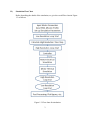
Simulation Flow Chart
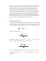
Before describing the details of the simulation, we give the overall flow chart in Figure
1.3 as follows:
Figure 1.3: Flow chart for simulation
3
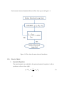
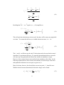
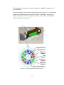
For the motor electrical simulation block, the flow chart is given in Figure 1.4.
Figure 1.4: Flow chart for motor electrical simulation
III.)
Electrical Model
1.
Dynamical Equations
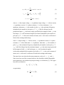
The motor dynamics are modeled by four primary dynamical equations in directquadrature reference frame (dq0):
u d  R s i d  Ld
4
did
  me Lq iq
dt
(1)
u q  Rs iq  Lq
diq
dt
  me Ld id   me  PM
 M  i q  p   PM  i d  Ld  Lq 
3
4


M L 
2
I me  c me 
p
(2)
(3)
(4)
where ud is direct input voltage, uq is quadrature input voltage, id is direct current,
iq is quadrature current, Rs is phase resistance, Ld is direct inductance, Lq is
quadrature inductance, p is the number of poles,  me is the mechanical frequency
multiplied by the number of pole pairs p / 2 ,  PM is the flux linkage from the
permanent magnet,  M is the motor torque generated by the magnetic fields,  L is the
load torque,  me is the mechanical angular acceleration multiplied by the number of
pole pairs p / 2 , I is the rotor's moment of inertia, and c is the rotor's coefficient of
friction from windage and bearings.
where u is input voltage, id is direct current, iq is quadrature current, Rs is phase
resistance, Ld is direct inductance, Lq is quadrature inductance, p is the number of
poles,  me is the mechanical frequency multiplied by the number of pole pairs p / 2 ,
 PM is the flux linkage from the permanent magnet,  M is the motor torque generated
by the magnetic fields,  L is the load torque,  me is the mechanical angular
acceleration multiplied by the number of pole pairs p / 2 , I is the rotor's moment of
inertia, and c is the rotor's coefficient of friction from windage and bearings.
The motor losses are related to the motor parameters, such as Rs , c , Ld , and L q .
Since losses have an effect on motor behavior, they should be modeled through the
motor parameters, not calculated in post-processing, as is often done [5]. The copper
loss can be calculated as


Pcu  ia  ib  ic R s ,
2
2
2
(5)
or equivalently
Pcu 


3 2
2
i d  i q Rs ,
2
5
(6)
for balanced 3-phases. In either case, note that the resistance is the parameter directly
associated with the power loss in the windings. Likewise, windage and bearing losses
are directly associated with the coefficient of friction, c . All iron losses (hysteresis,
classical eddy, and excess eddy losses) can be associated with the nonlinear
inductance, L .
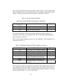
Much of the motor modeling research done in the past [1] and [8] and even recent
work [9] use constant parameter values in simulations, although some did use
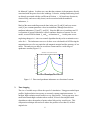
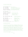
nonlinear inductances [2] and [7], and [10]. Since the BH curve is nonlinear and H
is a function of current, inductance is also a nonlinear function of current. For our
model, we used FEM to obtain Ld and Lq as functions of iq . At this point we are
neglecting changes in id since our control algorithm already seeks to maintain a zero
value for id . The inductance curves we do have were calculated in ANSYS using the
magnetization curve for our particular soft-magnetic material and the geometry of our
motor. The analysis was done for zero direct current and for a wide range of
quadrature currents (Figure 1.5).
Inductance as a Function of Current
5
Ld
Inductance, L , L [mH]
d
q
4.5
Lq
4
3.5
3
2.5
2
1.5
1
0.5
-300
-200
-100
0
100
Current, i [A]
q
200
300
Figure. 1.5. Direct and quadrature inductance as a function of current.
2.
Time Stepping
The size of variable arrays affects the speed of a simulation. Using prerecorded input
profiles, high resolution is necessary to accurately capture transient moments. A
uniform, high resolution would result in a very large profile. To keep our array sizes
small but maintain high resolution where needed, we used a line simplification
algorithm to reduce the number of points where little activity would occur. This
compression technique allowed us to reduce the profiles to less than 4% of their
original size.
6
That said, the electrical time constant is often much smaller than the time-step size of
the compressed profiles. Since the frequency of the electrical component of the
simulation is directly related to the first derivative of the input angular position
profile for the motor, we can dynamically scale the electrical time step nonuniformly. Therefore, we had two loops, one macro loop that stepped through the
elements of the profile and a nested micro loop with very small, but variable time
steps for the electrical equations. The result of this apparent complication was a
many-fold speed improvement. This is a tremendous advantage of not relying on
MATLAB built-in ODE solvers, which do not have the advantage of knowing how
big of a time step to take but must rather continually search for it.
3.
Field Oriented Control (FOC)
A thorough analysis of motor heat generation should include how the motor is driven.
Our control equations are derived from the primary simulation equations (1) through
(4). Starting with equation (4) and noting that in (3) iq can be factored out, we get
iq
M
iq
L 
2
I me  c me  ,
p
(7)
which can be rearranged to be
L 
iq 
2
I me  cme 
p
M
.
(8)
iq
At this point we reinterpret  me which is d me / dt to be e / dt , where e
me
me
is the
error in  me , with a tuning coefficient, k p , in front. This gives
L 
iq 
*
e

2
 Ik p me  c me * 


p
dt

M
,
(9)
iq
where iq is the desired current for the next time step and  me is the desired next*
*
step angular speed equal to  me  k p eme . Using (4) to substitute for  L in (9), we
arrive at (10):
7
iq
*


2
2
 M  I me  c me 
p
p

 
M
iq

.
e

2
 Ik p me  c me * 


t
p

(10)
M
iq


Recalling that  me   me equals k p eme , (10) simplifies to
*
iq  iq 
*
2
p
M
  eme

  me   c k p eme
 I  k p
t
 


 ,
(11)

iq
This will track the desired motor velocity well, but there will be some rotor angle drift
over time. To counter this drift error, we added a theta error term, k i e / dt :
me

*
iq  iq   k i

2


p M
iq
e me 

dt 
  eme


  me   c k p e me 
 I  k p
dt


 


(12)
The k p and ki coefficients are the only PI values that need to be tuned in the control
algorithm. For maximum efficiency, it is generally desired that the direct current be
zero since any flux generated in the direct axis would not contribute to torque.
However, direct current does not necessarily directly translate to direct flux. As the
following equation shows, direct current can contribute to useful torque if the direct
and quadrature inductances are not equal, as given in (3).
Most of the time, however, the desired direct current set point, id * , should be zero.
With the desired currents determined, the desired voltages can be found:
*
u d  R s i d  Ld
*
*
*
di d
*
* *
  me Lq iq
dt
8
(13)
u q  R s i q  Lq
*
*
*
di q
dt
*
  me Ld id   me  PM ,
*
*
*
*
(14)
*
where Ld * and Lq are based on the desired current values. It should be noted that
while many of the variables are updated based upon the desired currents,  M was not
updated for the control equations. This is a reasonable simplification since for a
round rotor  PM is independent of  me , id should normally be zero, and the iq factor
is divided out:
M
iq



3
p   PM  id  Ld  Lq 
4
(15)
For the non-round rotor case, our direct interpolation method could be used to include
the dependence on theta.
Even after the desired control values were calculated, the reality of limits (current and
voltage) needed to be included. Instead of directly capping those values, we realized
that the system converged more quickly and ran more smoothly if the functions used
were all smooth [11]. For our case, we used a segmented curve of first and secondorder polynomials.
IV.)
Thermal Model
1.
Model Setup
A lumped node thermal network is to represent the temperature of every solid part of
the EMA. The thermal resistances and capacitances between the nodes can be treated
as electrical resistances and capacitances. Hence the temperature of every node can be
solved as the voltage in this equivalent network (Table 1.1). This approach is well
developed in motor design industry [12, 13]. Some commercial motor design
software package has already included the thermal network simulation, i.e. MotorCAD [14]. Some studies have been made with FEA analysis and experimental testing
have shown that such an approach is valid [15].
Table 1.1 The analogy of equivalent thermal circuit
9
R  conductive 
R

convective
X
k * Acontact
1

h * Asurface
C    *V * C p
(16)
(17)
Equations (16) and (17) show how to calculate of the R and C values for simple onedimensional geometry. Accurate estimates for R and C values are not possible for
complicated geometries such as an electric motor. The traditional lumped node
thermal network is based on a “forward” direction modeling process. In this process,
with all the material, geometry and construction information provided, the thermal
resistance R and capacitance C are calculated based on empirical and theoretical
relations. For example, when the winding wire type, winding structure, potting
material, slot width and teeth thickness are given, the thermal resistance from winding
to stator and from winding to rotor can be calculated. Because this type of approach
requires large number of empirical relations to achieve high accuracy, a “reverse”
modeling process is introduced in this paper. A detailed 3-D solid model of a target
motor is constructed and imported to an FEA software like ANSYS [16] to perform
steady-state and transient simulation. With these results we can estimate and select
the values for the thermal resistances and capacitances. The advantage of this method
is that we can evaluate the fidelity of the lumped node model with a real motor, add
or reduce nodes to increase the model accuracy and efficiency, and estimate the
maximum error between the node temperature and maximum temperature in real
motor.
This procedure can also be extended to model the gear-box, motor-driver and drivetrain, and even include the aircraft wing surfaces and frames. The thermal network
can also be incorporated into a multi-physics model to simulate the electrical, thermal
and mechanical performance of the whole EMA and its supporting structure. Once
the proper thermal resistances and capacitances are selected, this simulation engine
can be used with various time dependent boundary conditions during the whole
mission duration, including the air temperature, aircraft speed, altitude and sunlight.
10
The computational requirement of such a simulation is negligible compared to the
FEA simulation.
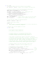
Due to the symmetry, the geometry of the model shown in Figure 1.1 is divided into a
quarter section and imported into ANSYS for the FEA simulation. The nodes are
numbered in Figure 1.6. These numbers are also the same as those in the lumped
node network shown in Figures 1.7.
Figure 1.6. Thermal node locations on motor.
11
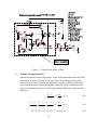
Figure 1.7. Lumped node model of EMA
2.
Dynamic Thermal Equations
After all the thermal resistor and capacitor values of the lumped-node network model
of the motor in Figure 5 are known, the same values of the thermal resistors and
capacitors can be used to simulate the temperature response of the motor parts with
any combination of heat losses and boundary conditions. For this standard resistorcapacitor electrical network, a set of first-order ordinary differential equations can be
written as:
U1  U 3
dU 1
 C1
 I C t 
dt
R1
(18)
U 4  U 3 U 10  U 3 U 1  U 3
dU 3


 C3
 I S t 
R3
R10
R1
dt
(19)
R9  R10 U 10
 U 3 R9  R10U 9  R9 R10 I W t 
12
(20)
U 6  U 8 U 13  U 8
dU 8

 C8
0
R6b
R8
dt
(21)
U 13  U 4 U 13  U 8
dU 13

 C13
 I BB t 
R13
R8
dt
(22)
U 14  U 4 U 13  U 4 U 4  U 3 U 4  U 5
dU 4



 C4
0
R4a
R13
R3
R4
dt
(23)
U 12  U 14 U 7  U 12
dU 12

 C12
 I BF t 
R12
R7
dt
(24)
U 9  U 6 U 10  U 9
dU 9

 C9
 I M t 
R6
R9
dt
(25)
U 6 U 7 U 6 U 8 U 9 U 6
dU 6


 C6
0
R6 a
R 6b
R6
dt
(26)
U 7  U 12 U 6  U 7
dU 7

 C7
 I R7a
R7
R6 a
dt
(27)
U 12  U 14 U 14  U 4
dU 14

 C14
 I R14
R12
R4a
dt
(28)
Because the time constant (about 10 ms) for the thermal component is much larger
than for the electrical component in our case, the thermal component was calculated
less often, thereby increasing the speed of the simulation.
V.)
References
1. Shi, K. L., Chan, T. F., Wong, Y. K., Ho, S. L. "Modeling and Simulation of
the Three-phase Induction Motor Using Simulink," Int. J. Elect. Enging. Educ.,
Vol. 36, pp. 163-172., Manchester U.P., Great Britain, 1999.
2. Lipo, Thomas A., Consoli, Alfio, "Modeling and Simulation of Induction
Motors with Saturable Leakage Reactances," IEEE Transactions on Industry
Applications, Vol. IA-20, No. 1, pp. 180-189, 1984.
13
3. Soe, Nyein N., Yee, Thet T. H., Aung, S. S., "Dynamic Modeling and
Simulation of Three-phase Small Power Induction Motor," World Academy of
Science, Engineering and Technology, Vol. 42, No. 79, pp. 421-424, 2008.
4. Otto, Jens, "Dynamic Simulation of Electromechanical Systems using ANSYS
and CASPOC," 2002 International ANSYS Conference, ANSYS, 2002.
5. Roshen, Waseem, "Iron Loss Model for PM Synchronous Motors in
Transportation," 2005 IEEE Conference on Vehicle Power and Propulsion, pp.
4, ISBN: 0-7803-9280-9, 2005.
6. Dolinar, D., Weerdt, R. De, Freeman, E. M., "Calculation of Two-axis
Induction Motor Model Parameters Using Finite Elements," IEEE
Transactions on Energy Conversion, Vol. 12, No. 2, pp. 133-142, 1997.
7. Topcu, E. E., Kamis, Z.,Yuksel, I., "Simplified numerical solution of
electromechanical systems by look-up tables," Mechatronics, Vol. 18, No. 10,
pp. 559-565, Elsevier, 2008.
8. Mohamed, M. A., Nagrial, M. H., "Modelling and Simulation of Vectorcontrolled Reluctance Motors Drive System," International Conference on
Simulation, No. 457, pp. 380-384, ISBN: 0-85296-709-8, 1998.
9. Sun, Fengchun, Li, Jian, Sun, Liqing, Zhai, Li, Cguo, Fen, "Modeling and
Simulation of Vector Control AC Motor Used by Electric Vehicle," Journal of
Asian Electric Vehicles, Vol. 3, No. 1, pp. 669-672, Asian Electric Vehicle
Society, 2005.
10. Demerdash, N. A., Gillott, D. H., "A New Approach for Determination of
Eddy Current and Flux Penetration in Nonlinear Ferromagnetic Materials,"
IEEE Trans. MAG-10, pp. 682-685, 1974.
11. Merzouki, R., Cadiou, J. C., "Estimation of backlash phenomenon in the
electromechanical actuator," Control Engineering Practice, Vol. 13, No. 8, pp.
973-983, Elsevier, 2004.
12. Mellor, P.H., Roberts, D., Turner, D. R., "Lumped parameter thermal model
for electrical machines of TEFC design", IEEE Proc-B, Vol 138, No5, Sept.
1991.
13. DiGerlando, A., Vistoilo, I., "Thermal network of induction motors for steady
state and transient operations analysis", ICEM 1994, Paris.
14. Motor-CAD v3.1.7, Motor Design Ltd, www.motor-design.com.
15. Y.K. Chin, D.A. Staton, "Transient thermal analysis using both lumped-circuit
approach and finite element method of a permanent magnet traction motor",
IEEE AFRICON 2004.
16. ANSYS V12.0., ANSYS, Inc., www.ansys.com.
14
Part II – User’s Manual I.)
Introduction
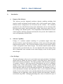
a.
Purpose of the Software
This software provides integrated non-linear dynamic modeling including both
electrical model and thermal model together with a field oriented control scheme.
Different motor configurations can be entered into the software. The simulation
provides the user with all the necessary motor information, such as: mission profile
following, motor torque, motor current, phase voltage, input power, power losses in
the windings, and a thermal profile. This comprehensive and detailed look at motor
control together with heat generation and transfer will provide solid foundation for
users to design highly efficient EMAs.
b.
Software Capability
Package of a nonlinear dynamic modeling of a permanent magnet motor that
describes both the control and thermal performance of the motor in following highly
transient mission profiles. One of the most attractive features of this model is that it
is able to incorporate various motor designs. The software manual assumes that the
mission profile is provided to the user. For users familiar with control coding will be
able to manipulate some constants in the control helping to tune for their specific
motor designs.
c. User Privileges
The main advantages to the user is to put in their own motor parameters for alternate
designs and test whether the design is capable of providing proper control and also
find out the thermal performance. The motor parameter code (located in Appendix
A) contains a variety of values that must be determined by the user if an alternate
design is used. Values such as phase resistance, number of magnetic poles, and the
moment of inertia must be determined. Motor limitations are also set in this file to
ensure that these limits are not exceeded during operation. The inductance values, as
well as the thermal resistance and capacitance values, can be obtained from FEM
models. If a new motor model is to be used that maintains the non-linear nature of the
simulation, the new inductance values, thermal resistance and capacitance, should be
recalculated using FEM. Although determining these values is outside the scope of
15
this manual, the user is able to manipulate any of the data inside the motor simulation
to suit the needs of their design.
II.)
Input Parameters
There are the two file names ‘motorParameter’ and ‘missionProfile.xlsx’ for input
motor parameters and mission profiles.
motorParameters.m contains motor parameters specific to a particular motor design as
well as calculated parameters. If you are to change the name of this folder or make a
new motor design, the new name of the folder must be input into the main program.
The code is displayed in Part IV but these parameters show the motor parameters for
this particular example. These values can be changed to accommodate other
motor/EMA designs.
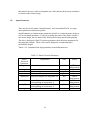
Tables 2.1-2.4 summarize the input parameters in motorParameters.m.
Table 2.1. Motor Electrical Parameters
Motor
Electrical
Parameters
Rs_room
p
I
c
lambdaPM
LdSN
LqSN
iq
Explanations
Units
Source
phase resistance at room temperature

number of poles
inertia moment of rotor
friction coefficient
permanent magnet flux amplitude PM
kg m2
kg m2/s
Wb
FEM or
Measurement
Given
Given
Given
FEM or
Measurement
FEM or
Measurement
FEM or
Measurement
Given
array of direct inductance Ld
corresponding to current array iq
array of quadrature inductance Lq
corresponding to current array iq
array of quadrature current
16
H
H
A
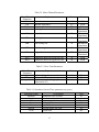
Table 2.2. Motor Thermal Parameters
Motor Thermal
Explanations
Parameters
Rth
thermal resistance
Cth
thermal capacitance
Troom
room temperature
IC
winding loss
Units

Source
IS
stator loss
W
IW
winding loss
W
IBB
rear bearing loss
W
IBF
front bearing loss
W
IM
magnet loss
W
conduction heat loss to gear box axle
conduction heat loss to gear box case
W
W
FEM
FEM
Given
Electrical
Simulation
Electrical
Simulation
Electrical
Simulation
Mechanical
Simulation
Mechanical
Simulation
Electrical
Simulation
FEM
FEM
Units
Source
rad/m
Given
Given
Given
IR7a
IR14
CW
J/oC
o
C
W
Table 2.3. Drive Train Parameters
Drive Train
Parameters
Ncr
effDrive
theta_meIntial
Explanations
total coupling ratio
drive train efficiency
initial rotor angle multiply p/2
when stroke is 0
rad
Table 2.4. Simulation Limits (These parameters are given.)
Simulation Limits
xMinLim
xMaxLim
tauMLim
uLim
iLim
didtLim
vLim
Explanations
minimum value of stroke
maximum value of stroke
motor torque limit
voltage limit
current limit
current change rate limit
speed limit
17
Units
m
m
Nm
V
A
A/s
m/s
Excel file missionProfile.xlsx provides data for mission profile. The mission profile
data is assumed to have been provided already and is not subject for discussion in this
manual. The input parameters in mission profile is summarized in Table 5.
Table 2.5. Mission Profile Parameters
(may come from aerodynamic measurement or simulation)
Mission Profile
Parameters
tN
xSN
FLN
Explanations
array for time
array for stroke profile
array for load force profile
Units
s
M
N
Due to the fact that there can be various mission profiles and motor designs it is
important to ensure that your file names in the ‘FOC’ folder match the file names as
represented in the code above.
There are also input parameters used to set up simulation. These parameters are
summarized in Table 2.6.
Table 2.6. Simulation Parameters (These parameters are given.)
Simulation Parameters
spc
tauTh
kp
ki
alpha_dt
epsilon
Ncvg
Explanations
samples per cycle of highest frequency
thermal time constant
proportional parameter for PI controller
integral parameter for PI controller
forward time-stepping weight for
implicit algorithm in electrical loop
error for electrical convergence loop
maximum number of convergence
iterations
Units
s
A s/rad
If the experience of the user is adequate in the design of the control scheme, there are
few parameters that can be changed to decrease error in the ability for the motor to
follow the flight profile data. Users can change the proportional constant, or kp value,
and the integral constant, or ki value of the control.
18
Two parameters, alpha_dt and beta_dt located in the main code are weighted averages
used in calculating next step values. Generally the beta value is set to .5 but can be
altered at the user’s discretion for algorithm convergence. Another parameter that
can be changed to help improve design is spc or samples per frequency as shown
below.
19
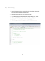
III.)
Software Startup
1.
Once all the proper m-files are verified click on the ‘Start Menu’ and open the
MATLAB software through the program listing.
2.
Once MATLAB is open go to ‘File’ and click on ‘Open’
3.
Go to through the above mentioned directory path to find the ‘FOC’ folder
4.
Click on the ‘FOC’ folder and then click on the file name ‘FOC.m’
5.
The following code should be displayed in the MATLAB editor screen
20
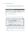
IV.)
Software Execution and Procedure
1. In order to run the simulation you can either click in the editor window and press
the F5 shortcut key, or click the run button at the top of the editor window.
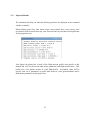
2. The following menu will pop up to add the foc.m file to the MATLAB path.
 Click Change Directory. Different versions of MATLAB will show different
popup boxes when the directory is not specified. Simply ensure that all the files
needed to run the program are located in the same folder before changing the
path.
3. The simulation will begin running. The runtime will vary based on the system.
21
There will be a statistical report and a total of 9 graphs displayed as well once the
simulation is finished.
V.)
Output Parameters
The Output parameters are summarized in Tables 2.7 and 2.8 for reporting statistics and
plot figures.
Table 2.7. Output Parameters to Report Statistics
Parameters
PcuMean
tauMMax
FMax
vMax
aMax
dtMax
dtEMax
dtEMin
Explanations
mean winding copper loss
maximum motor torque
maximum actuator force
maximum actuator velocity
maximum acceleration
maximum macro time step
maximum electrical time step
minimum electrical time step
Units
W
Nm
N
m/s
m/s2
s
s
s
Table 2.8. Output Parameters in Figures
Output Parameters
tNR
xN
tauMN
udN
uqN
idN
iqN
PcuN
PinN
TthN
Explanations
array for output time sequence
array for actual stroke
array for motor torque
array for direct voltage
array for quadrature voltage
array for direct current
array for quadrature current
array for instantaneous copper loss
array for instantaneous input power
2D array for temperature at different
nodes
22
Units
s
m
Nm
V
V
A
A
W
W
o
C
VI.)
Expected Results
The simulation has fully run when the following statistics are displayed in the command
window to include:
Mean winding power loss, max motor torque, max actuator force, max velocity, max
acceleration, min electrical time step, max electrical time step and the total elapsed time
for the program to run.
Also figures are plotted are a result of the flight mission profile used specific to this
manual and will vary based on other motor parameters and flight mission data. This
profile was a five minute section of a full flight profile. Acceptable values will be
specific each set of parameters or profile data; however, some generalizations can be
made about parameters such as power loss.
23
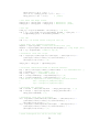
1. The stroke profile shows that movement of the shaft in the EMA. The green line
represents the actual movement of the actuator based on the mission profile. The blue
line is the desired movement of the EMA. It is hard to see the blue because the green
is covering indicating good control. The desired stroke is in excel file
missionProfile.xlsx. The actual stroke is saved in strokeActual.xlsx.
Mechanical Stroke Following
2.6
xdesired
2.4
xactual
2.2
Stroke, x [in]
2
1.8
1.6
1.4
1.2
1
0.8
0
0.5
1
1.5
2
2.5
3
Time, t [min]
3.5
4
4.5
5
Figure 2.1 (a): EMA stroke
To further see the accuracy of the stroke following plot, a zoomed section of Figure 1
is shown below.
24
Mechanical Stroke Following
2.4
xdesired
xactual
2.2
2
Stroke, x [in]
1.8
1.6
1.4
1.2
1
0.8
0.35
0.4
0.45
0.5
Time, t [min]
0.55
0.6
0.65
Figure 2.1 (b): Zoomed section of stroke
2. In the following Figure 2.2 (a) and (b), the load force from mission profile and load
torque converted by
L 
FLoad
N cr drive
where Ncr is coupling ratio and driveis drive train efficiency. In Figure 2.2 (c), the
magnetic torque is shown. Comparing Figure 2.2 (b) and (c), we found they are close.
This is because the moment of inertia of the motor we used is small. The magnetic
torque and load torque are related by:
J
d 2 m
  M  L
dt 2
The magnetic torque is saved in Excel file tauM.xlsx.
25
Load Force
3000
2000
Load Force, F
load
[N]
1000
0
-1000
-2000
-3000
0
0.5
1
1.5
2
2.5
3
Time, t [min]
3.5
4
4.5
5
Figure 2.2(a): Load Force
Load Torque
2
1.5
0.5
L
Load Torque,  [N m]
1
0
-0.5
-1
-1.5
-2
0
0.5
1
1.5
2
2.5
3
Time, t [min]
3.5
Figure 2.2(b): Load Torque
26
4
4.5
5
Magnetic Torque
2.5
2
M
Magnetic Torque,  [N m]
1.5
1
0.5
0
-0.5
-1
-1.5
-2
-2.5
0
0.5
1
1.5
2
2.5
3
Time, t [min]
3.5
4
4.5
5
Figure 2.2(c): Magnetic Force
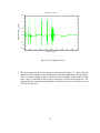
3. The dq currents provided to the motor are represented in Figure 2.3. Notice that the
current id nearly constant around 0 and doesn’t exceed the dotted blue line limitations.
This is a proper reading as direct current does not contribute to the rotation of the
rotor. Only iq contributes to the torque as seen by the variation in the green line. The
dotted green lines represent current limits of the motor. The current results are saved
in Excel file idiq.xlsx.
27
dq Currents
4
id
3
iq
Currents, id [A] and iq [A]
2
1
0
-1
-2
-3
-4
0
0.5
1
1.5
2
2.5
3
Time, t [min]
3.5
4
Figure 2.3: Direct and quadrature currents
28
4.5
5
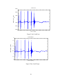
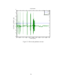
4. The direct and quadrature voltages are shown here in Figure 2.4 and are similar to the
currents. The direct voltage should remain around 0 and the quadrature voltage
should contribute to the requirements of the selected flight profile.
dq Voltages
80
ud
60
uq
Voltages, ud [V] and uq [V]
40
20
0
-20
-40
-60
-80
0
0.5
1
1.5
2
2.5
3
Time, t [min]
3.5
4
4.5
5
Figure 2.4 (a): Direct and quadrature voltages
The ud voltage does not vary too much and generally stays around zero as seen in the
zoomed section of the graph. The voltage results are saved in Excel file uduq.xlsx.
29
dq Voltages
ud
60
uq
Voltages, ud [V] and uq [V]
40
20
0
-20
-40
-60
0.9
0.95
1
1.05
Time, t [min]
1.1
1.15
Figure 2.4 (b): Zoomed in Section of Direct and Quadrature Voltages
30
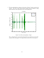
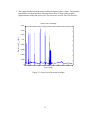
5. The copper winding inside the motor contain the highest source of heat. The transient
heat analysis is represented here with peak values near 12 Watts which is much
higher than the steady state power loss. The results are saved in Excel file Pcu.xlsx.
Power Loss in Windings
0.016
0.014
Power Loss, Pcu [kW]
0.012
0.01
0.008
0.006
0.004
0.002
0
0
0.5
1
1.5
2
2.5
3
Time, t [min]
3.5
4
Figure 2.5: Power loss in the motor windings
31
4.5
5
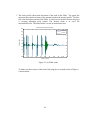
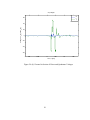
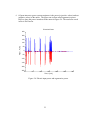
6. Of great interest to power systems engineers is the power in (positive values) and out
(negative values) of the motor. The power out is often called regenerative power.
Here we show the power in and out of the motor in Figure 2.6. The results are saved
in Excel file Pin.xlsx.
Electrical Power
250
200
150
Power, P [W]
100
50
0
-50
-100
-150
-200
-250
0
50
100
150
Time, t [min]
200
250
Figure 2.6: Electric input power and regenerative power
32
300
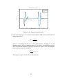
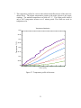
7. The temperature profiles for various nodes taken from different areas of the motor are
shown below. The highest temperatures pertain to the nodes closest to the copper
windings. The ambient temperature was held at 22 °C. This flight profile showed
only a 0.4ºC temperature increase over 5 minute period. The results are saved in
temperature.xlsx.
Temperature Distribution
22.4
22.35
Temperature, T [C]
22.3
22.25
22.2
22.15
22.1
22.05
22
0
0.5
1
1.5
2
2.5
3
Time, t [min]
3.5
Figure 2.7: Temperature profile of the motor.
33
4
4.5
5
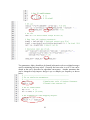
Part III – Source Code (foc.m) %
%
%
%
%
%
%
%
%
Nonlinear Dynamic Modeling and Field Oriented Control
of Permanent Magnet (PM) Motor
Written in SI or MKS Unit System.
Authors:
David Woodburn
Dr. Lei Zhou
Dr. Thomas X. Wu
clear all; close all; clc;
tic;
% -----------------------% Input motor parameters.
% -----------------------motorParameter
% ------------------------% Load EMA mission profile.
% ------------------------Mission = xlsread('missionProfile.xlsx'); % Load into mission profile
tN = Mission(:,1).'; % time sequence
xSN = Mission(:,2).'; % stroke sequence
FLN = Mission(:,3).'; % load force sequence
% xSN = xSN * 0.0254; % If stroke is in inch, needs to convert to meter.
% FLN = FLN * 4.4482; % If load force is in lbf, needs to covert to Newton.
theta_meSN = xSN*Ncr*p/2 + theta_meInitial;
tauLN = FLN/(Ncr*effDrive); % Load torque [N m]
% ---------------------------------------------------% Set up simulation parameters.
% ---------------------------------------------------spc = 10;
% Samples per cycle of highest frequency
tauTh = 0.01;
% Thermal time constant [s]
% Set PI coefficients.
kp = 0.1;
% []
ki = 0.0001; % [A s/rad]
% Set differential time-stepping weights.
alpha_dt = 0.5;
beta_dt = 1 - alpha_dt;
% Set motor simulation convergence parameters.
epsilon = 0.0001;
% Convergence limit []
Ncvg = 50;
% Maximum number of convergence iterations
T = tN(end) - tN(1);
% T could have been redefined.
34
Nt = length(tN);
% Initial length of profile arrays
nfMax = 1;
% Order of highest frequency harmonic of interest
NtR = round(spc*(nfMax*omega_meLim/(2*pi))*T); % High-res, time steps
dtE0 = T/(NtR-1);
% Mean hi-res time step
omegaSMin = 2*pi/0.002; % Min sampling frequency [rad sample/s]
omegaSMax = 2*pi/dtE0; % Max sampling frequency [rad sample/s]
ntR = 2;
% Hi-res index for recording []
NtETotal = 1; % Counter for the total number of simulation points
tTh = 0;
% Last time for thermal calculation [s]
% Pad arrays (for interpolation referencing). Lengths are Nt+3.
dtBar = mean(diff(tN)); % Note that dt might not be constant.
tN = [tN(1)-dtBar, tN, tN(end)+dtBar, tN(end)+2*dtBar];
theta_meSN = [theta_meSN(1), theta_meSN, theta_meSN(end), theta_meSN(end)];
tauLN = [tauLN(1), tauLN, tauLN(end), tauLN(end)];
% Initialize states.
Rs = Rs_room;
%
id = 0;
%
iq = 0;
%
did_dt = 0;
%
diq_dt = 0;
%
Initial
Phase d
Phase q
Rate of
Rate of
Ld0 = LdSN(1);
Lq0 = LqSN(1);
Ld = Ld0;
Lq = Lq0;
Ld at zero current
Lq at zero current
Initial Ld
Initial Lq
%
%
%
%
ud = 0;
uq = 0;
theta_me = theta_meSN(1);
omega_me = 0;
alpha_me = 0;
Qs = 0;
Q = zeros(Nth,1);
NConverge = 0;
%
%
%
%
%
%
%
%
phase winding resistance [ohm]
current [A]
current [A]
change of id [A/s]
change of iq [A/s]
Phase d voltage [V]
Phase q voltage [V]
Start up (Mechanical angle)*p/2 [rad]
(Mechanical angular frequency)*p/2 [rad/s]
(Mechanical angular acceleration)*p/2 [rad/s^2]
Heat source flux (from windings)
Heat flux
Counter for number of convergence iterations
% Saturation curve points.
rSat = 0.10;
% Saturation ratio []
i1 = iLim*(1-rSat); % Beginning of current saturation [A]
i3 = iLim*(1+rSat); % Ending of current saturation [A]
u1 = uLim*(1-rSat); % Beginning of voltage saturation [V]
u3 = uLim*(1+rSat); % Ending of voltage saturation [V]
th2L = xMinLim*Ncr*p/2 + theta_meInitial; % theta_me max limit
th2R = xMaxLim*Ncr*p/2 + theta_meInitial; % theta_me min limit
th0 = (th2R + th2L)/2;
% Midpoint between theta_me limits
th1R = (th2R - th0)*(1-rSat) + th0;
th3R = (th2R - th0)*(1+rSat) + th0;
th1L = -(th0 - th2L)*(1-rSat) + th0;
th3L = -(th0 - th2L)*(1+rSat) + th0;
% Set threshold to show limits in plots.
limThreshold = 0.8; % []
35
% ---------------------------% Initialize recording arrays.
% ---------------------------% Initialize hi-res arrays.
NtR0 = round(NtR*1.05);
%
tR = zeros(1,NtR0);
%
uaR = zeros(1,NtR0);
%
ubR = zeros(1,NtR0);
%
tauLR = zeros(1,NtR0);
%
theta_meR = zeros(1,NtR0); %
omega_meR = zeros(1,NtR0); %
% Initialize low-res arrays.
tNR = zeros(1,Nt);
theta_meN = zeros(1,Nt);
theta_meN(1) = theta_meSN(1);
omega_meN = zeros(1,Nt);
idN = zeros(1,Nt);
iqN = zeros(1,Nt);
phiN = zeros(1,Nt);
Add 5%
Hi-res
Hi-res
Hi-res
Hi-res
Hi-res
Hi-res
buffer [].
time record [s]
phase A voltage record [V]
phase B voltage record [V]
load torque record [N m]
theta_me record [rad]
omega_me record [rad/s]
% Actual theta_me [rad]
%
%
%
%
Actual omega_me [rad/s]
Direct current [A]
Quadrature current [A]
Torque angle [rad]
LdN = zeros(1,Nt); LdN(1) = Ld0;
LqN = zeros(1,Nt); LqN(1) = Lq0;
% Direct inductance [H]
% Quadrature inductance [H]
udN = zeros(1,Nt);
uqN = zeros(1,Nt);
RsN = zeros(1,Nt); RsN(1) = Rs;
tauMN = zeros(1,Nt);
PinN = zeros(1,Nt);
PcuN = zeros(1,Nt);
PfricN = zeros(1,Nt);
TthN = zeros(Nth,Nt); TthN(:,1) = Tth;
% Direct voltage [V]
% Quadrature voltage [V]
% Resistance [ohm]
% Machine torque [N m]
% Power in [W]
% Copper loss [W]
% Friction loss [W]
% Temperature [C]
% ----------------------% Run through time steps.
% ----------------------%
%
%
%
%
%
%
%
%
%
%
%
%
A low resolution (low-res) profile is analyzed one segment (step) at a
time, breaking each segment into many sub-segements that have a high
resolution. Interpolation is used to accomplish this, and the number
and size of the time steps are based on an average hi-res time step
size based on the maximum electrical speed of the motor. During
playback, there is only one low-res segment (Nt = 2) and all the
profile points are hi-resolution. At that point, the hi-res time step
size and the number of time steps are based on the pre-recorded hi-res
time array. Any technique used for interpolating omega on the low-res
scale will be yield different results than on the hi-res scale just
because of the scale, even if the same technique is used. However,
using a perfect N-point derivative (PNPD) should yield fairly accurate
results without averaging.
% For each low-res segment, simulate.
36
for nt = 2:Nt
% Calculate number and size of steps for this segment.
dt = tN(nt+1) - tN(nt); % Update low-res segment time-step size.
% Calculate variable, hi-res time step based on dthetaE/dt.
dtheta_me = theta_meSN(nt+1) - theta_meSN(nt);
dtheta_meAbs = abs(dtheta_me);
omegaSAbs = spc*dtheta_meAbs/dt; % spc = samples per cycle
omegaSAbs = omegaSAbs*(omegaSAbs>omegaSMin) + ...
omegaSMin*(omegaSAbs<=omegaSMin);
omegaSAbs = omegaSAbs*(omegaSAbs<omegaSMax) + ...
omegaSMax*(omegaSAbs>=omegaSMax);
dtE = 2*pi/omegaSAbs;
NtE = ceil(dt/dtE) + 1; % Update number of sub, hi-res time points.
dtE = dt/(NtE-1);
% Update hi-res segments time-step size.
% Count the total number of simulation points.
NtETotal = NtETotal + (NtE - 1);
% Reset micro-loop's energy.
PcuBar = 0;
%
This is used to find the average power in a micro loop which is
%
then used for the thermal component.
% Simulate this low-res segment in hi-res.
for ntE = 2:NtE
% ------------------------------% Get inputs to motor simulation.
% ------------------------------% Variables ending in "S" represent desired values.
% Variables ending in "P" represent next step values.
% Variables without these are this step's values.
%
%
%
%
%
%
%
The process of getting the inputs to the motor simulation
transitions from this time step to the next. The inputs belong
to the resolved (convergent) state of the next time step.
Therefore, udP, uqP, tauLP, thetaEP, and omegaEP all belong to
the next time step. The motor simulation accepts certain of
those inputs as given values and then resolves the remaining
states of the motor such that those inputs could be true.
% Determine index in Nt scale from index in NtE scale.
wt = ntE/NtE; % Progress in this nt segment (0 to 1]
% Use weighting to get t, thetaS, and omegaS.
t = tN(nt)*(1-wt) + tN(nt+1)*wt;
%
tauLP = tauLN(nt)*(1-wt) + tauLN(nt+1)*wt;
%
theta_meS = theta_meSN(nt)*(1-wt) + theta_meSN(nt+1)*wt; %
dt3 = tN((nt):(nt+2)) - tN((nt-1):(nt+1));
%
omega_me3 = (theta_meSN(nt:(nt+2)) - ...
theta_meSN((nt-1):(nt+1)))./dt3;
% [rad/s]
omega_meS = (wt <= 0.5).*(omega_me3(1).*(0.5 - wt) + ...
37
[s]
[N m]
[rad]
[s]
omega_me3(2).*(0.5 + wt)) + ...
(wt > 0.5).*(omega_me3(2).*(1.5 - wt) + ...
omega_me3(3).*(wt - 0.5));
% [rad/s]
% Get theta and omega errors.
eTheta_me = (theta_meS - theta_me); % Mechanical [rad]
eOmega_me = (omega_meS - omega_me); % Mechanical [rad/s]
% Get iqS.
tauM_iq = 3*p/4*(lambdaPM + id*(Ld-Lq)); % [N m/A]
iqS = iq + 2/(p*tauM_iq)*(I*(kp*eOmega_me/dtE - alpha_me) + ...
c*(kp*eOmega_me)) + ki*eTheta_me/dtE; % [A]
% Set idS.
idS = 0; % id should almost always be zero [A]
% Rate limit iqS (reduces transients).
diqdtS = (iqS-iq)/dtE; % Predicted current rate [A/s]
diqdtS = sign(diqdtS)*min([didtLim,abs(diqdtS)]); % Cap diqdt [A/s]
iqS = iq + diqdtS*dtE; % Rebuilt iqS [A]
% Saturation limit abs of iqS.
iqS = sign(iqS)*((abs(iqS)<i3)*(abs(iqS) - (abs(iqS)>=i1)*...
((abs(iqS)-iLim*(1-rSat))^2)/(4*iLim*rSat)) + ...
(abs(iqS)>=i3)*iLim); % [A]
omega_meP = omega_me + (kp*eOmega_me);
% Calculate inductances based on desired currents.
mLq = (NL-1)*(abs(iqS)-iLMin)/(iLMax-iLMin) + 1;% Unbounded real []
wLq = mod(mLq,1); % Real number [0:1) []
nLq = mLq - wLq; % Unbounded integer []
LdS = (1-wLq)*LdSN(nLq) + wLq*LdSN(nLq+1); % [H]
LqS = (1-wLq)*LqSN(nLq) + wLq*LqSN(nLq+1); % [H]
% The above is equivalent to using interp1, but much faster.
%
LdS = interp1(iL,LdSN,abs(iqS));
%
LqS = interp1(iL,LqSN,abs(iqS));
% Calculate new voltages.
udS = Rs*idS + LdS*(idS-id)/dtE
uqS = Rs*iqS + LqS*(iqS-iq)/dtE
omega_meP*lambdaPM; % [V]
- omega_meP*LqS*iqS; % [V]
+ omega_meP*LdS*idS + ...
% Saturation limit abs of voltages.
ud = sign(udS)*((abs(udS)<u3)*(abs(udS) - (abs(udS)>=u1)*...
((abs(udS)-uLim*(1-rSat))^2)/(4*uLim*rSat)) + ...
(abs(udS)>=u3)*uLim); % [V]
uq = sign(uqS)*((abs(uqS)<u3)*(abs(uqS) - (abs(uqS)>=u1)*...
((abs(uqS)-uLim*(1-rSat))^2)/(4*uLim*rSat)) + ...
(abs(uqS)>=u3)*uLim); % [V]
% -----------------------------------------% Seek convergence for one hi-res time step.
38
% -----------------------------------------% Assume next values from present values. Simulation should not
% assume any knowledge of "S" values.
idP = id + did_dt*dtE; % [A]
iqP = iq + diq_dt*dtE; % [A]
alpha_meP = alpha_me; % Angular acceleration [rad/s^2]
omega_meP = omega_me + alpha_me*dtE;
% Run dynamical equations until convergence.
for nConverge = 1:Ncvg
% Get
mLq =
wLq =
nLq =
LdP =
LqP =
% The
%
%
next inductances by look-up table.
(NL-1)*(abs(iqP)-iLMin)/(iLMax-iLMin) + 1;%Unbounded real
mod(mLq,1); % Real number [0:1) []
mLq - wLq; % Unbounded integer []
(1-wLq)*LdSN(nLq) + wLq*LdSN(nLq+1); % [H]
(1-wLq)*LqSN(nLq) + wLq*LqSN(nLq+1); % [H]
above is equivalent to using interp1, but much faster.
LdP = interp1(iL,LdSN,abs(iqP));
LqP = interp1(iL,LqSN,abs(iqP));
% Get next magnetic and air torques. p/2 is used to get
% cummulative torque, not to convert to electrical units.
tauMP = 3*p/4*iqP*(lambdaPM + idP*(LdP-LqP));
% [N m]
tauFricP = c*omega_meP*2/p; % [N m]
% Get next angular acceleration.
alpha_meP = p/2/I*(tauMP - tauLP - tauFricP);
% [rad/s^2]
% Comes from tauM = tauL + I*alpha_m, alpha_me = alpha_m*p/2.
% Get next angular speed and angle.
omega_meP = omega_me + ...
(alpha_dt*alpha_me + beta_dt*alpha_meP)*dtE; % [rad/s]
theta_meP = theta_me + ...
(alpha_dt*omega_me + beta_dt*omega_meP)*dtE; % [rad]
% theta_meP is updated here because some parameters might
% depend on the value of theta_me.
% Get next currents. Current should be updated last since it
% is used for the convergence test.
didP_dt = 1/LdP*(-Rs*idP + omega_meP*LqP*iqP + ud); % [A/s]
diqP_dt = 1/LqP*(-Rs*iqP - omega_meP*LdP*idP + uq - ...
omega_meP*lambdaPM);
% [A/s]
idP = id + (alpha_dt*did_dt + beta_dt*didP_dt)*dtE; % [A]
iqPOld = iqP;
iqP = iq + (alpha_dt*diq_dt + beta_dt*diqP_dt)*dtE; % [A]
% Check for electrical convergence.
if abs(iqP - iqPOld)/iLim < epsilon % []
break;
end
end % end nConverge
39
% Add convergence iterations.
NConverge = NConverge + nConverge;
% Update heat generated.
Pcu = 3/2*(iq^2 + id^2)*Rs; % Next-step source heat [W]
PcuBar = PcuBar + Pcu/NtE;
% ----------------% Simulate thermal.
% ----------------if t - tTh > tauTh
% Get next-step winding resistance.
Rs = Rs_room;
dtTh = t - tTh;
tTh = t;
% Calculate temperatures.
IC = Pcu/4; % winding loss (only quarter portion is used)
% Calculate next-step temperatures.
TthP(1) = Tth(1) + (IC + (Tth(3)-Tth(1))/Rth(1))/Cth(1)*dtTh;
TthP(2) = Tth(2);
TthP(3) = Tth(3) + (IS + (Tth(4)-Tth(3))/Rth(2) + ...
(Tth(10)-Tth(3))/Rth(12) + (Tth(1)-Tth(3))/Rth(1))/Cth(3)*dtTh;
TthP(4) = Tth(4) + ((Tth(4)-Tth(14))/Rth(3) + ...
(Tth(13)-Tth(4))/Rth(14) + (Tth(3)-Tth(4))/Rth(2) + ...
(Tth(5)-Tth(4))/Rth(4))/Cth(4)*dtTh;
TthP(5) = (Rth(5)*Tth(4) + Rth(4)*Tth(2))/(Rth(4)+Rth(5));
TthP(6) = Tth(6) + ((Tth(9)-Tth(6))/Rth(6) + ...
(Tth(7)-Tth(6))/Rth(7) + (Tth(8)-Tth(6))/Rth(8))/Cth(6)*dtTh;
TthP(7) = Tth(7) + (-IR7a + (Tth(6)-Tth(7))/Rth(7) + ...
(Tth(12)-Tth(7))/Rth(9))/Cth(7)*dtTh;
TthP(8) = Tth(8) + ((Tth(6)-Tth(8))/Rth(8) + ...
(Tth(13)-Tth(8))/Rth(10))/Cth(8)*dtTh;
TthP(9) = Tth(9) + (IM + (Tth(6)-Tth(9))/Rth(6) + ...
(Tth(10)-Tth(9))/Rth(11))/Cth(9)*dtTh;
TthP(10) = (Tth(3)*Rth(11) + Tth(9)*Rth(12) + ...
Rth(11)*Rth(12)*IW)/(Rth(11)+Rth(12));
TthP(12) = Tth(12) + (IBF + (Tth(14)-Tth(12))/Rth(13) + ...
(Tth(7)-Tth(12))/Rth(9))/Cth(12)*dtTh;
TthP(13) = Tth(13) + (IBB + (Tth(4)-Tth(13))/Rth(14) + ...
(Tth(8)-Tth(13))/Rth(10))/Cth(13)*dtTh;
TthP(14) = Tth(14) + (-IR14 + (Tth(4)-Tth(14))/Rth(3) + ...
(Tth(12)-Tth(14))/Rth(13))/Cth(14)*dtTh;
Tth = TthP;
end
% -------------% Update states.
% --------------
40
id = idP;
iq = iqP;
did_dt = didP_dt;
diq_dt = diqP_dt;
Ld = LdP;
Lq = LqP;
theta_me = theta_meP;
omega_me = omega_meP;
alpha_me = alpha_meP;
% -----------------------% Record hi-res variables.
% -----------------------tHR(ntR) = t;
udH(ntR) = ud;
uqH(ntR) = uq;
theta_meR(ntR) = theta_me;
omega_meR(ntR) = omega_me;
tauLR(ntR) = tauLP;
ntR = ntR + 1;
end % end hi-res simulation
% ------------------------% Record low-res variables.
% ------------------------% Store time.
tNR(nt) = t;
% Store motor stroke.
theta_meN(nt) = theta_me; % [rad]
omega_meN(nt) = omega_me; % [rad/s]
% Store currents.
idN(nt) = id; % [A]
iqN(nt) = iq; % [A]
% Store inductances.
LdN(nt) = Ld; % [H]
LqN(nt) = Lq; % [H]
% Store voltages.
udN(nt) = ud; % [V]
uqN(nt) = uq; % [V]
% Store resistance.
RsN(nt) = Rs; % [ohm]
% Store motor torque.
tauMN(nt) = tauMP; % [N m]
% Store powers [W].
41
PinN(nt) = 3/2*(iq*uq + id*ud); % Input power
PcuN(nt) = 3/2*(iq^2 + id^2)*Rs; % Copper loss for whole motor
PfricN(nt) = tauFricP*(omega_me*2/p);
% Store temperatures.
TthN(:,nt) = Tth;
end % End time stepping.
% Unpad profile arrays.
tN = tN(2:(Nt+1));
theta_meSN = theta_meSN(2:(Nt+1));
tauLN = tauLN(2:(Nt+1));
tR(ntR:end) = [];
theta_meR(ntR:end) = [];
omega_meR(ntR:end) = [];
tauLR(ntR:end) = [];
% ---------------% Show statistics.
% ---------------disp('Dynamic Modeling and Field Oriented Control of PM Motor');
% Calculate stroke, speed, and acceleration.
xN = (theta_meN - theta_meInitial)*2/p/Ncr;
vN = diff(xN)./diff(tNR);
NT = length(tNR);
tNRmid = (tNR(1:NT-1) + tNR(2:NT))/2;
aN = diff(vN)./diff(tNRmid);
% [m]
% [m/s]
% [s]
% [m/s^2]
% Calculate and Report statistics.
PcuMean = mean(PcuN);
% mean winding power loss [W]
tauMMax = max(abs(tauMN));
% [N m]
tauLMax = max(abs(tauLN));
% [N m]
FMax = tauLMax*Ncr*effDrive; % [N]
vMax = max(abs(vN));
% [m/s]
aMax = max(abs(aN));
% [m/s^2]
dtEMin = min(diff(tHR));
% [s]
dtEMax = max(diff(tHR));
% [s]
spaces = '';
disp([spaces 'Mean winding power loss = ' num2str(PcuMean) ' W ']);
disp([spaces 'Max motor torque = ' num2str(tauMMax) ' N m ']);
disp([spaces 'Max actuator force = ' num2str(FMax) ' N ']);
disp([spaces 'Max velocity = ' num2str(vMax) ' m/s ']);
disp([spaces 'Max acceleration = ' num2str(aMax) ' m/s^2 ']);
disp([spaces 'Min electrical time step = ' num2str(dtEMin) ' s ']);
disp([spaces 'Max electrical time step = ' num2str(dtEMax) ' s ']);
% -----------% Show graphs.
% -----------% Stroke
42
figure('Name','Stroke');
plot(tN/60, xSN/0.0254, tNR/60, xN/0.0254);
xlswrite('strokeActual.xlsx', [tNR;xN].');
ylabel(['Stroke, \it{x}\rm [in]']);
xlabel('Time, \it{t}\rm [min]');
title('Mechanical Stroke Following');
legend('\it{x_{desired}}','\it{x_{actual}}');
% Torque
figure('Name','Load Force')
plot(tN/60,FLN);
ylabel('Load Force, \it{F_{load}}\rm [N]');
xlabel('Time, \it{t}\rm [min]');
title('Load Force');
figure('Name','Load Torque');
plot(tN/60, tauLN);
ylabel('Load Torque, \it{\tau_L}\rm [N m]');
xlabel('Time, \it{t}\rm [min]');
title('Load Torque');
figure('Name','Magnetic Torque');
plot(tNR/60, tauMN, 'g');
xlswrite('tauM.xlsx', [tNR;tauMN].');
ylabel('Magnetic Torque, \it{\tau_M}\rm [N m]');
xlabel('Time, \it{t}\rm [min]');
title('Magnetic Torque');
% Current
figure('Name','Current');
plot(tNR/60,idN,tNR/60,iqN);
xlswrite('idiq.xlsx', [tNR;idN;iqN].');
ylabel('Currents, \it{i_d}\rm [A] and \it{i_q}\rm [A]');
xlabel('Time, \it{t}\rm [min]');
title('dq Currents');
legend('\it{i_d}','\it{i_q}');
% Voltage
figure('Name','Voltage');
plot(tNR/60,udN, tNR/60,uqN);
xlswrite('uduq.xlsx', [tNR;udN;uqN].');
% xlswrite('uduq.xlsx', [tHR;udH;uqH].'); % for high resolution, very slow
ylabel('Voltages, \it{u_d}\rm [V] and \it{u_q}\rm [V]');
xlabel('Time, \it{t}\rm [min]');
title('dq Voltages');
legend('\it{u_d}','\it{u_q}');
% Copper Loss
figure('Name','Copper Loss');
plot(tNR/60,PcuN/1000);
xlswrite('Pcu.xlsx', [tNR;PcuN].');
ylabel('Power Loss, \it{P_{cu}}\rm [kW]');
xlabel('Time, \it{t}\rm [min]');
title('Power Loss in Windings');
43
% Electric Power
figure('Name','Electric Power');
xlswrite('Pin.xlsx', [tNR;PinN].');
PinNN = [];
tNN = [];
n0 = 1;
hold on;
for n = 1:length(tNR)-1
PinNN = [PinNN, PinN(n)];
tNN = [tNN, tNR(n)];
if PinN(n)*PinN(n+1) < 0
PinNN = [PinNN, 0];
tadd = tNR(n)+(tNR(n+1)-tNR(n))*abs(PinN(n))/...
(abs(PinN(n))+abs(PinN(n+1)));
tNN = [tNN,tadd];
if PinN(n) > 0
plot(tNN/60,PinNN,'b');
else
plot(tNN/60,PinNN,'r');
end
PinNN = 0;
tNN = tadd;
end
end
PinNN = [PinNN, PinN(end)];
tNN = [tNN, tNR(end)];
if PinN(end) > 0
plot(tNN/60,PinNN,'b');
else
plot(tNN/60,PinNN,'r');
end
ylabel('Power, \it{P}\rm [W]');
xlabel('Time, \it{t}\rm [min]');
title('Electrical Power');
hold off;
% Thermal
figure('Name','Thermal');
plot(tNR/60,TthN([1,2,3,4,5,6,7,8,9,10,12,13,14],:));
xlswrite('temperature.xlsx', [tNR;TthN;].');
ylabel('Temperature, \it{T}\rm [C]');
xlabel('Time, \it{t}\rm [min]');
title('Temperature Distribution');
toc;
44
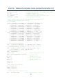
Part IV – Motor Parameter Code (motorParameter.m) % Define primary motor parameters.(This example is for a Danaher's motor.)
Rs_room = 0.775;
% Phase resistance at room temperature [ohm]
p = 10;
% Number of poles []
I = 113.2*10^(-6);
% Inertia moment [kg m^2/rad]
c = 0.00001;
% Friction Coefficient [kg m^2/s rad]
lambdaPM = 0.0793;
% PM flux amplitude [Wb]
% Build direct inductance Ld and quadrature inductance Lq.
% Load current and inductance arrays.
iL = 0:10:300;
LdSN = [4.46928937, 4.435673396, 4.334488681, 4.201478319, ...
4.055221239, 3.895196891, 3.741845461, 3.59804698, ...
3.464592095, 3.34851825, 3.250656076, 3.16810712, ...
3.096573444, 3.033981034, 2.978679457, 2.929048419, ...
2.884038304, 2.843532188, 2.805950657, 2.77189558, ...
2.739726553, 2.710652474, 2.683562881, 2.658379174, ...
2.634980767, 2.612739765, 2.592141217, 2.572607466, ...
2.553992315, 2.536488402, 2.519800427] * 0.001; % [H]
LqSN = [4.612083555, 4.52697855, 4.276907416, 3.919619295, ...
3.518989894, 3.09915783, 2.740369271, 2.445203741, ...
2.199031273, 1.99252454, 1.823051455, 1.684390442, ...
1.568691069, 1.470728535, 1.386369068, 1.313170018, ...
1.249202936, 1.192423128, 1.141458078, 1.095896561, ...
1.054610808, 1.017268661, 0.98309393, 0.951930145, ...
0.923114329, 0.896516968, 0.871994934, 0.84926359, ...
0.828084863, 0.808445183, 0.789983231] * 0.001; % [H]
% Define thermal parameters.
Rth = [0.001389; 0.007697; 0.5; 0.001896; 16.0; 0.08577; ...
9.1358; 16.97; 4.4581; 4.4; 5.933; 37.49; 2.6; 2.6];
% Thermal Resistance [^o C/W]
Cth = [38.85; 0; 82.3; 159.11; 0; 56.03; 14.99; 7.08; ...
6.72; 0.00176; 0; 13.18; 8.41; 62.56];
% Thermal Capacitance [J / ^o C]
Nth = length(Rth);
Troom = 22;
% Room Temperature [^o C]
Tth = ones(length(Rth),1)*Troom;
IS = 0;
% stator loss
IW = 0;
% winding loss
IBB = 0;
% rear bearing loss
IBF = 0;
% front bearing loss
IM = 0;
% magnet loss
IR7a = 0;
IR14 = 0;
% Get current min and max.
NL = length(iL);
iLMin = min(iL);
iLMax = max(iL);
% Define gear train coupling ratio.
Ncr = 49.8728/0.0254;
% Total Coupling Ratio [rad/m]
45
effDrive = 0.76;
% Drive train efficiency []
theta_meInitial = pi/6;% Rotor initial (mechanical angle*p/2)when stroke=0.
kAir = 0.00180297/(2*pi)^1.927/(2*pi*(p*pi)^0.927);
% Define simulation limits.
xMinLim = 0;
% stroke min [m]
xMaxLim = 4.05*0.0254;
% stroke max [m]
tauMLim = 1.9256;
% Motor torque limit [N m]
PLim = 688;
% Rated output power [W]
uLim = 165;
% Maximum instantaneous voltage allowed per phase [V]
iLim = 19.2;
% Maximum instantaneous current allowed per phase [A]
didtLim = 5*10^4;
% Maximum current change rate allowed [A/s]
vLim = 0.086;
% Maximum speed allowed [m/s]
omega_meLim = vLim*Ncr*p/2; % Maximum mechanical angular speed *p/2 [rad/s]
46