Download User Manual - Thomas Kunz

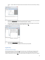
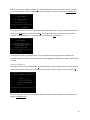
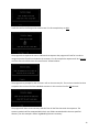
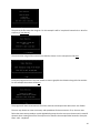
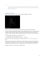
Statistics for
Dynamic & Static Networks
User Manual
Supervising Professor: Thomas Kunz
An ongoing project with contributions by Evan Bottomley, Cristopher Briglio, Jordan Edgecombe
(Dynamic Statistics for NS2 Networks, version 1) and Hussain Saeed (Statistics of Static Networks)
Version 3
Carleton University
Summer 2014
Table of Contents
ABOUT ................................................................................................................................................................... 3
TITLE SCREEN ......................................................................................................................................................... 3
LOCATION GENERATOR ............................................................................................................................................ 3
DYNAMIC STATISTICS ............................................................................................................................................... 3
STATIC STATISTICS ................................................................................................................................................... 4
STATISTICAL SUMMARY ............................................................................................................................................ 4
SPREADSHEET CREATOR ............................................................................................................................................ 4
FULL STATISTICAL RUN THROUGH ............................................................................................................................... 5
ANIMATION GRAPHS ............................................................................................................................................... 5
BUILDING THE PROGRAM ...................................................................................................................................... 5
REQUIRED SOFTWARE .............................................................................................................................................. 5
SETUP .................................................................................................................................................................. 5
VISUAL STUDIOS SETTINGS ........................................................................................................................................ 6
RUNNING THE PROGRAM ...................................................................................................................................... 6
TOPOLOGY.XML ...................................................................................................................................................... 7
Location Generation ....................................................................................................................................... 7
Dynamic Statistics .......................................................................................................................................... 8
GraphViz Visualization ................................................................................................................................... 9
HIGHMOBILITY..................................................................................................................................................... 10
Full Statistical Run Through .......................................................................................................................... 10
Statistics Summary ....................................................................................................................................... 11
Spreadsheet ................................................................................................................................................. 13
VERYDENSE .......................................................................................................................................................... 13
Static Statistics............................................................................................................................................. 13
ANIMATION & GRAPHS .......................................................................................................................................... 15
STATISTICS CALCULATED...................................................................................................................................... 16
THE AVERAGE NUMBER OF NODE NEIGHBOURS IS: ......................................................................................................... 16
THE NODE(S) WITH THE MOST NEIGHBOURS IS/ARE:....................................................................................................... 17
THE NUMBER OF NODES THAT THE NODE(S) WITH THE MOST NODE NEIGHBOURS HAVE IS: ....................................................... 17
THE AVERAGE PATH LENGTH FOR ALL SOURCE-DESTINATION PAIRS (IN METERS): .................................................................... 17
THE AVERAGE PATH LENGTH FOR ALL SOURCE-DESTINATION PAIRS (IN HOPS): ....................................................................... 17
THE NETWORK DIAMETER (IN METERS): ...................................................................................................................... 17
THE NETWORK DIAMETER (IN HOPS): ......................................................................................................................... 18
TOTAL NUMBER OF COMPONENTS: ............................................................................................................................ 18
NODE(S) WITH THE HIGHEST BETWEENESS CENTRALITY: .................................................................................................. 18
LINKS ADDED/LINKS BROKEN: .................................................................................................................................. 18
LINK CHANGES: .................................................................................................................................................... 18
COVERAGE (IN %): ................................................................................................................................................ 18
NEIGHBOURHOOD INSTABILITY: ................................................................................................................................ 18
CLUSTERING COEFIICIENT: ....................................................................................................................................... 18
DEGREE OF RANDOMNESS/PREDICTABILITY: ................................................................................................................ 18
ISSUES OR HELP ................................................................................................................................................... 20
2
About
Statistics for Dynamic & Static Networks is a program written and compiled in C++. The program creates
statistics from dynamic and static network simulations of NS2, Opnet and Core formats using the Boost
Graph Library. The program also uses MATLAB, GraphViz, and Excel to help visualize, organize and
interpret the statistics.
Title Screen
Each aspect of the program is access through the title screen contained in main.cpp. The title screen
allows user to choose which of the various components of the program to run.
Location Generator
Location Generator can interpret NS2, Opnet and Core dynamic network simulations. It gives the user
the choice to generate an output file for single or multiple files at a time. In the case of multiple files, the
user must specify a folder location for the program to look through. After locating the file(s) specified,
the program will create an output folder for the scenario(s). The name of the folder has the format:
'*scenario file name* output'. The program then reads in the scenario and generates each nodes
location every second until the node becomes static, retaining the longest run time needed for the
network to become static. This information is the written to a file in a specific format.
Dynamic Statistics
Dynamic Statistics reads the user specified output file from the Location Generator and creates statistics
for the user chosen run time in intervals of the given refresh rate. Using the Boost Graph Library the
following statistics are created:











Average number of neighbors each node has
The nodes that have the most neighbors
The average distance between nodes
The number of components
The network diameter
The nodes with the highest betweeness centrality
The number of links changed
The coverage of the combined nodes over time
The network instability
The clustering coefficients
The degree of randomness/predictability
The statistics are then written to their own separate files within the output folder. It also gives the
option to create a graphViz visualization of the network at any given multiple of the refresh rate.
3
Static Statistics
The Static Statistics portion of the program (originally written by Hassain Saeed) reads in static network
scenarios of NS2, Opnet and Core formats. It then generates basic statistics for these files which include:
 Average number of neighbors each node has
 The nodes that have the most neighbors
 The average distance between nodes
 The number of components
 The network diameter
 The nodes with the highest betweeness centrality
The statistics are then written to their own separate files within an output folder. It also gives the
option to create a graphViz visualization of the network.
Statistical Summary
The Statistical Summary part of the program creates averaged statistics from multiple scenarios. The
program works by reading the statistics generated from Dynamic Statistics or Static Statistics for several
specific files and creates a summary of these statistics in a separate folder. The following statistics are
summarised:








average number of neighbors each node has
the average distance between nodes
the number of components
the network diameter
the number of links changed
the percent coverage of the area
the average neighbourhood instability
the average clustering coefficient
(Links summary isn't included for static scenario summaries).
Spreadsheet Creator
The Spreadsheet Creator uses the statistics created in Dynamic Statistics or Static Statistics, as well as
Statistical Summary part of the program to create a spreadsheet that can be opened in Microsoft Office
Excel. The spread sheet brings together the specific data from all the scenarios in a visually friendly way.
It relies on the 'files.txt' output from Statistical Summary in order to identify what files to include. The
spreadsheet includes the following data (for dynamic scenarios):
 Average links created and broken per second
 Total links created and broken in desired run time
 Number of connected components (at initial and final time)
 Average number of neighbours (at initial and final time)
 Average path length in hops (at initial and final time)
 Network diameter in hops (at initial and final time)
For static scenarios:
4




Number of connected components
Average number of neighbours
Average path length in hops
Network diameter in hops
This portion of the program only works on NS2 scenarios with file names with the format: 'Scenario##.txt'
Full Statistical Run Through
This portion of the program simply runs the user through the Location Generator then automatically
created statistics for the file(s) using Dynamic Statistics without having the user give the desired file to
run the statistics on.
Animation Graphs
Animation Graphs is a program created in MATLAB that uses the statistics created in Dynamic Statistics
for a particular scenario to create an animation of the nodes and their trajectories over time on an x-y
plain for the user desired run time as well as several graphs illustrating all the statistics. Note that only
the average clustering coefficient and neighbourhood instability are graphed, instead of the per-node
results.
Building the Program
Required Software
Visual Studios 2012
http://msdn.microsoft.com/library/dd831853.aspx
Boost Graph Library 1.54.0
http://www.boost.org/doc/libs/1_54_0/libs/graph/doc/index.html
GraphViz 2.30.1
http://www.graphviz.org/Download.php
MATLAB R2013a
http://www.mathworks.com/help/matlab/index.html
Microsoft Office Excel 2007
http://office.microsoft.com/en-ca/excel/
Setup
(At current stage of program is only compatible with windows, built using Microsoft Visual Studios 2012)

In Visual Studio’s File menu, select New -> Project. Then in the new window that pops up, under
Visual C++, select Win32 Console Application.
5

Delete the premade source and header files (right click -> exclude from project) and add all the
necessary source and header files to the project. This includes:
- Main.cpp
- Dynamic Statistics.cpp
- Location Generator.cpp
- Static Statistics.cpp
- SpreadsheetCreator.cpp
- stdafx.cpp
- stdafx.h
- convert.h
- targetver.h

Apply all the required settings. The Property pages can be opened by selecting View -> Property
Manager, then clicking the wrench symbol in the upper left corner.
Visual Studios Settings
The following are the setting that must be configures in Visual Studious 2012 in order to run the
program:
Configuration Manager - Configuration - Release
Solution Configurations - Release
Property Pages - Configuration Properties - General - Character Set - Not Set
Property Pages - Configuration Properties - C/C++ - Precompiled Headers - Not Using
(make sure Configuration is set to: All Configurations)
Add Boost library (boost_1_54_0 folder) to Additional Included Directories found in:
Property Pages - Configuration Properties - C/C++ - General - Additional Included Directories

After this you simply build the project and start the program
Running The Program
The following is a run through of the program using these example files:

Examples - Dynamic - Opnet - topology.xml
(Single dynamic scenario)

Examples - Dynamic - NS2 - HighMobility
(Multiple dynamic scenarios)

Examples - Static - NS2 - verydense
(Multiple static scenarios)
With the following examples the user should learn to run any aspect of the program.
(Different aspects of the program that are being shown may have been altered or changed since these
pictures were taken as the program was further worked on. Also, these pictures may not depict the
program running for these specific examples, please follow the written instructions to get the same
results as the examples and not what the visuals show)
6
topology.xml
Location Generation
After starting the program, choose option 1 (Location Generator) from the title screen.
After coming to the Location Generator main menu, the user must choose the proper file type, which in
this example is OPNET.
The user must then specify whether the location generation will be for one or multiple files, in this
example there is one file (1).
When running for one file, the user must enter the name of the given file he/she wishes to run the
program on. In this example the file is 'topology.xml'.
7
The user must then enter the transmission range and refresh rate of the scenario to be used when
creating the statistics. In this example the transmission range will be 1000 and the refresh rate will be 1.
The program will then require the values of the x and y axis for the network to be used in the Matlab
section of the program (only for Opnet scenarios). In this example both axis will be 5000.
The program will then run through the location generation for the specific file and output it to its own
output folder.
Dynamic Statistics
Once the location generation is complete, exit this section and go back to the title screen. Next choose
option 2 (Dynamic Statistics). The user must then enter the path and name of the output folder and file
generated in the last step. For this example the user must input 'topology output\topology_out.txt'.
8
The program will then prompt the user to enter the run time that the statistics will be generated for. For
this example the run time should be 1800.
The program will then ask if the user wants to create a graphViz visualization of the scenario. If the user
chooses yes, the user must enter the time at which the visualization will be created. The time of the
visualization must be less than the run time, a multiple of the refresh rate and greater than 0. For this
example a visualization will be created at time 1000.
The Statistics for this scenario have now been created. The output can be found in the example folder
located in: Examples - Dynamic - Opnet - topology output
GraphViz Visualization
Once the GraphViz visualization has been
created, the user must now use a separate
program to create a photo of it. Within GraphViz,
the gvedit.exe application can be used to read
and output the visualizations. To start you must
locate and open this application (found in:
graphviz-2.30.1\release\bin\ gvedit.exe ). Once
running, have the program open the file by going
to file -> open. Once the application has open
the file (graphViz_1000.dot) the user must then
have it output the visualization as a picture.
There are a few ways to do this although the
easiest seems to be the following:

Hit the Layout button, this button is
located near the top left and has the shape of a man running. It can also be found within
9
Graph - > Layout. Within the Output Console at the bottom of the screen it should say: working
on...




Next hit the Settings button located next to the layout button which looks like the layout button
but with a blue box in it. It can also be found within Graph -> Settings.
Once clicked it will bring up a menu name Dialog. Make sure its Layout Engine is dot, the Scope
is graph, and specify your desired output file type then click OK
Then click the Layout button two more times
The visualization has now been output in the format that you specified
HighMobility
Full Statistical Run Through
After starting the program, choose option 7 from the title screen. This will bring you through the Full
Statistical Run Through version of the program. Once at the Location Generator menu, choose the
proper file type which in this case is NS2. Then specify whether the program will run for one or multiple
10
files, for this example it will be multiple (2). Then indicate the directory that contains all the scenarios.
For this example that will be the HighMobility folder located in c drive for simplicity (c:\HighMobility).
The program will then ask for the transmission range and refresh rate. In this example the transmission
range will be 250 and the refresh rate will be 1. The program will then ask for the run time that the
statistics will be generated for. For this example it will be run for 150 seconds.
The program will then run through all the ‘.txt’ files (because NS2 file type) within the folder and
generate statistics on them. It will automatically create a graphViz visualization for each scenario at the
run time.
Statistics Summary
Next from the title screen choose option 4 (Statistics Summary). The program will then ask you if you're
running the summary for dynamic scenarios or static scenario. For this example it will be dynamic (2).
The user must then specify the directory the files are located. For this example it is same directory as
before (c:\HighMobility).
11
It will then ask for the file type the scenarios are. For this example they are NS2.
The program then requires the user to indicate what sequence the program will look for in order to
recognize that the file will be included in the summary. For this example the sequence will be 'Scenario'
as all the files in the folder have the name format: 'Scenario#-#.txt'.
The program then prompts for the run time it will run the summary for. The run time must be less than
or equal to the run time of all the individual scenarios. In this case it will run for 150 seconds.
The program will then create summary statistics from all the files that match the sequence. The
summary statistics will be outputted within their own folder contained within the user specified
directory. For this example it will be 'HighMobility\Scenario.summary'.
12
Spreadsheet
Once the summary has been created choose option 5 (Spreadsheet Creator) from the main menu. The
program will ask if the spreadsheet will be created for dynamic or static scenarios. For this example it
will be dynamic (2). The program will then ask for the directory that the files are located which is the
same as before (c:\HighMobility).
The program will then ask for the sequence used to create the summary files (Scenario).
The program will then create an ‘.xml’ spreadsheet for all the files used in the summary and output it to
the summary folder. The file outputted for this example (Scenario.spreadsheet.xml) can be found in the
example folder located in: Examples - Dynamic - NS2 - HighMobility - Scenario.summary
verydense
Static Statistics
From the title page choose option 3 (Static Statistics). This will bring the user to the Static Statistics
menu where it will require the file type that file(s) will be. For this example it is NS2.
The program will then ask if it will run for a single or multiple files. For this example it will be multiple.
(2)
13
The path to the files must then be given. For this example it will be 'verydense' located in the c drive for
simplicity (c:\verydense).
The transmission range of the network must then be chosen. For this example it will be 250.
Finally the program will ask if the user wishes to create a graphViz visualization along with the statistics.
For this example the answer will be yes.
The program will then create statistics for all the scenarios and output them within their own folders.
The user may choose to create a summary and spreadsheet for these scenarios. If so, the user must
follow the exact same procedure as with HighMobility except that the user must choose static instead of
dynamic when creating these files. The output can be found in the example folder located in: Examples Static - NS2 - verydense
14
Note:
This section only explains the very basics needed to run each section of the program and only
specifies the requirements that the user must input in order to run. See Documentation file for
more specific requirements.
Animation & Graphs
If the user chooses option 6 from the title screen the following will be displayed.
The user must open animations_graphs.m within matlab to use this portion of the program.
Once the user has opened animations_graphs.m within MATLAB, the user must run it by typing into the
command window 'animations_graphs()'. The program will then ask for the path to the output file
(created in Location Generator). Once specified the program will ask for the run time of the animation.
The program will then create the animation of the scenario along with various graphs visualizing the
various statistics in respect to time. These can then be saved in a variety of formats. The following are
the graphs created for testscen.txt with an animation than ran to 52 seconds that can be found in:
Examples - Dynamic - NS2 - testscen output - Matlab output
15
Statistics Calculated
This section will explain what each of the statistics created through the program mean and how they
were calculated. (This section was originally written by Hussain Saeed and Jordan Edgecombe).
The average number of node neighbours is:
What it means: Two nodes are considered neighbours if they directly connect with each other,
or in other words, if they share an edge with each other.
How it was calculated: In NS2 and Opnet, an edge is made when two nodes’ coordinates are
within the transmission range from one another, and in Core it is made when the two nodes
share the same WLAN. With Boost Graph Library, a vertex iterator can be made that can loop
through every unique node in the network. For each node, Boost Graph Library can then use an
edge iterator to see how many other nodes it is directly connected to. Each connection is then
16
recorded in a counter variable, and eventually this variable gets divided by the total number of
nodes to get the average number of node neighbours.
The node(s) with the most neighbours is/are:
What it means: The nodes that share the most connections with other nodes in the network
How was it calculated: While the vertex iterator loops through every single node, the ones that
have the most node neighbours are picked out and stored in a specific array. Then, after the
vertex iterator is done, this array just gets outputted.
The number of nodes that the node(s) with the most node neighbours have is:
What it means: The nodes with the most node neighbours have this number of connections
How it is calculated: While the array for the nodes with the most neighbours is being created,
another array is made to store the number of neighbours that the nodes with the most
connections have. One element of this array then gets simply outputted for this statistic.
The average path length for all source-destination pairs (in meters):
What it means: This is the average shortest distance along the edges between any two nodes,
regardless of whether or not they are directly connected to each other. To imagine what
‘shortest distance along the edges’ means, let’s say node 1 and node 3 are not connected and
that the path between them that goes through node 2 is shorter in distance than every other
possible node path between them. So let’s imagine that node 1 is connected to node 2 by an
edge that is 200 meters long and node 3 is connected to node 2 by an edge that is 150 meters
long. This program will say the distance between nodes 1 and 3 is 350 meters, no matter what
the straight line distance between them truly is.
How it is calculated: When the program reads through the input file, it takes in the x and y
coordinates for every node. Using these coordinates, the distances between directly connected
nodes are then calculated and are saved as edge weights. Then, using a Boost Graph Library
function called dijikstra_shortest_path and the vertex iterator again, the distance along the
edges between any two nodes is calculated and added to a total-sum variable. This variable is
then divided by the total number of all possible edges to get the average.
The average path length for all source-destination pairs (in hops):
What it means: This is the average minimum number of edges that exists between any two
nodes.
How it is calculated: The same way as was calculated in meters, except that instead of the edge
weights being the actual distances between the nodes’ coordinates, all of the edge weights are
set to 1.
The network diameter (in meters):
What it means: The longest ‘shortest distance along the edges’ between any two nodes,
regardless of whether or not they are directly connected to each other.
How it is calculated: While the dijikstra_shortest_path function found the shortest distance
along the edges between any two nodes, an if-statement was created that said that if the
shortest path was greater than the previous longest shortest path (originally set at 0 meters),
17
then that would become the new longest ‘shortest path along edges’. After every path was
calculated, the last path to become the new longest shortest path was then seen to be the
greatest and was then output.
The network diameter (in hops):
What it means: The largest minimum number of edges that exists between any two nodes.
How it is calculated: The same way as calculated in meters, except that instead of the edge
weights being the actual distances between the nodes’ coordinates, all of the edge weights are
set to 1.
Total number of components:
What it means: A component is a set of nodes that are all reachable to one another through a
path of edges.
How it is calculated: This statistic is calculated simply through Boost Graph Library’s
connected_components function.
Node(s) with the highest betweeness centrality:
What it means: This statistic shows the nodes that have highest amounts of shortest paths from
one node to another passing through them.
How it is calculated: Using a vertex iterator again and the Boost Graph Library function known as
brandes_betweeness_centrality, the betweeness centrality is calculated for every node in the
network. Then the nodes with the greatest values get put into a separate array, which then gets
outputted.
Links Added/Links Broken:
What it means: This statistic shows the number of links added/broken at every second of the
simulation.
How it is calculated: Using Pythagorean Theorem, the distance between each pair of nodes is
calculated. If this distance is less than or equal to the transmission range, then a link exists
between the pair.
An array of 1’s and 0’s tracks where these links exist. If a link is added, then the array has a 1 at
that point (ex: if node 0 and node 1 are connected, array[0][1] = 1 and array[1][0]=1). If a link is
broken then a 0 is placed at that point. If an entry goes from 1 to 0, then broken links is
increased by 1 and if an entry goes from 0 to 1 then added links is increased by 1.
Link Changes:
What it means: It is the amount of times a link gets broken or created for each node throughout
the simulation.
How it is calculated: This is simply calculated by having an array keeps track of every link change
per node by adding 1 every time a link has been added or created for that node while another
integer increments itself by two's every time a link is created or broken (by two because if a link
is always broken or created for two nodes).
18
Coverage (in %):
What it means: It is the percent of the defined area that has been passed through by a node at
any point in time
How it is calculated: The area is divided into a virtual grid, represented by a two-dimensional
array. During each cycle, each node increases the array value corresponding to its location by 1.
The coverage percent is determined by determining how many parts of the array have a value
greater than 0, then dividing that by the total parts and multiplying by 100. The final array is
outputted at the bottom, giving a general impression of where the nodes are concentrated as
well as allowing for depictions through MATLAB surface graphs. A separate output
(surface_graph) gives a format that can be copied into MATLAB as an array for easy visualization
of the node distribution.
Neighbourhood Instability:
What it means: It is the approximate rate at which the nodes create and break links.
How it is calculated: The instability is calculated for each node by determining how many links
were created and broken with that node, divided by the number of neighbours it has at that
point in time. The output is given in 10-cycle periods, starting with the 0-9 period. A final value
giving the average instability of all nodes over the entire period is listed at the bottom. A
separate output (average_instability) gives the average of the nodes at each point in time.
Clustering Coefficient:
What it means: It is the ratio of radio links among neighbours and the number of neighbours.
How it is calculated: The clustering coefficient is calculated for each node by determining how
many links there are between neighbours of the node, divided by the number of neighbours it
has at that point in time. A final value giving the average coefficient of all nodes over the entire
period is listed at the bottom. A separate output (average_clustering) gives the average of the
nodes at each point in time.
The Wikipedia page http://en.wikipedia.org/wiki/Clustering_coefficient provides a decent
summary of how exactly this is determined.
Degree of Randomness/Predictability:
What it means: It is a value indicating the transition probability between states.
How it is calculated: The area is divided into a virtual grid (similar to coverage, but less
segments), each part of which has a separate subgrid surrounding it (represented by a 4D array).
Whenever a node moves, it records the starting and ending grid location, and increments values
in the corresponding main grid (starting) and subgrid (ending). At the end, it tallies up the grid
values and determines the chance of a node going from any given grid segment to another one,
then uses the equation 𝐻 = −(𝑝𝑖 𝑄𝑖𝑗 𝑙𝑛𝑄𝑖𝑗 ), where pi is the probability to stay at the starting
location i and Qij is the probability to transition from state i to state j. The H values for each
segment of the main grid are summed up and averaged, giving the final output.
19
Issues or Help
See the Documentation file for more specific information on the different aspects of the program.
20