1
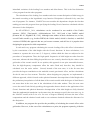
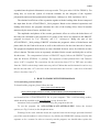
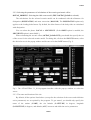
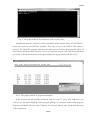
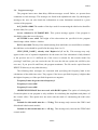
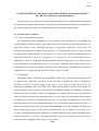
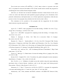
12062
ATLANTIDA3.1_2014 FOR WINDOWS:
A SOFTWARE FOR TIDAL PREDICTION
E. Spiridonov, O. Vinogradova, E. Boyarskiy, and L. Afanasyeva
Schmidt Institute of Physics of the Earth, Russian Academy of Sciences, ul. B. Gruzinskaya 10,
Moscow, 123995 Russia, e-mail: [email protected]
In this paper, we describe the possibilities of the ATLANTIDA3.1_2014 software, which
was recently developed for predicting tidal parameters on the Earth. These possibilities include
the calculation of the gravimetric oceanic effect, the amplitude delta-factors for oceanless Earth,
as well as the modeled amplitude factors and phase shifts for the Earth with ocean. The program
also calculates the tidal series. We present the highlights of the program and discuss the
underlying theoretical and methodical ideas. The detailed installation guidelines and user manual
are presented. The results of the calculations are compared with the observations.
INTRODUCTION
At present, there are about ten programs for calculating the prognostic delta-factors and
phase shifts of the tides as well as oceanic gravimetric effect. Among the first group of the
software, the most popular are the PREDICT program of the ETERNA package developed by
Wenzel [Wenzel G., 1996], T-soft [Van Camp & Vanterin, 2005], and MT80w programs [ICET].
The calculations of the oceanic effect are conducted by the LOAD97 (ETERNA 3.3) [Francis O.
and Mazzega P., 1990], GOTIC2 [Matsumoto et al., 2001], OLFG [Scherneck, 1991], and
SPOTL programs [Agnew, 1996, 1997].
The detailed intercomparison of these programs and the analysis of their performance
against the ATLANTIDA3.1._2014 program fall beyond the scope of the present work.
However, we briefly outline the main features of our program, which distinguish it from the
previous programs.
First, for calculating the Love numbers and delta-factors of the body tides, we applied the
latitudinal dependences of these parameters obtained in [Spiridonov E.A., 2014]. These
dependences differ from those calculated by Dehant V. et al. [1999] for the DDW/NH model.
Our curves have a somewhat steeper latitudinal gradient, which is particularly important in the
prediction of tidal data at high latitudes (see Fig. 6). The latitudinal dependence used in our work
does not depend on the form of the tidal or loading potential. Besides, we also calculated the
12062
12063
latitudinal variations of the loading Love numbers and delta-factors. This is the first distinction
of our program from the other programs.
The calculations of the loading Love numbers take into account dissipation of tidal energy in
the mantle according to the logarithmic creep function. Dissipation is allowed for by some but
not all programs. For instance, LOAD97 does not consider this dependence despite the fact that
nothing prevents this program from specifying the loading Green's functions calculated with the
allowance for the dissipation.
In ATLANTIDA3.1_2014, calculations can be conducted in two models of the Earth's
structure: PREM
[Dzeiwonski, A.M.&Anderson, D.L., 1981] and a later IASP91 model
[Kennett B.L.N., Engdahl E.R., 1991]. Although some authors in their calculations use, in fact,
several Earth's models (e.g., besides PREM, the 1066A model, which is obsolete) or modified
versions of PREM, this approach has not yet become common, and still less is it popular when
designing the programs for tidal computations.
In each and every program calculating the oceanic loading effect, this effect is determined
by the convolution of the tidal height with the Green's functions. In these calculations, it is
common to separate the near zone (2–5 degrees), within which the data are subjected to the
procedure of interpolation. Thus, the high spatial frequencies of tidal height are taken from the
near zone, whereas the data falling beyond this area are coarsely described by the values at the
grid nodes of the oceanic model. In our opinion, this approach is not quite reasonable because,
first, the high-frequency components affect the entire Earth and, therefore, they should be
calculated over the entire surface. Second, instead of the near zone, it is the far zone that
provides the largest contribution to the modeled oceanic gravimetric effect, and the calculations
for the far zone are less accurate. Therefore, when designing our program, we implemented a
different approach, which is based on the spherical harmonic decomposition of tidal height after
the preliminary interpolation of all the data of the oceanic models with the degree of detail that is
not worse than in the near zone in the calculations of the other authors. Thus, the near zone
covers the entire Earth. Strictly speaking, the approaches that are based on the application of the
Green's functions and spherical harmonic decomposition of the tidal height are fully identical
from the mathematical standpoint. At the same time, the attempt to specify the near zone (e.g. in
the LOAD97 model) with a size of a few tens of degrees infinitely increases the time of the
computations and the obtained result tends to our estimates obtained without the allowance for
the dissipation.
In addition, our program also provides the possibility of calculating the oceanic effect at the
grid nodes. However, in the case of the calculations at a point, the program separately yields the
12063
12064
loading and Newtonian (direct attraction) components of the oceanic effect as well as their sum.
By no means all programs provide this option.
In contrast to almost all the other programs of this kind, ATLANTIDA3.1_2014 has a
intuitively transparent user-friendly interface, which enables the user to run the program
straightforwardly, without referencing to the manual.
In the first section of this work, we discuss the general principles of the program and the
physical sense of the corresponding computational procedures. The second section, in fact,
presents the user's manual. Finally, in the third part, we show some results of our calculations
and compare the output of our program to the observations.
1. MAIN COMPUTATIONAL PROCEDURES
The general flow-chart of the calculations that are carried out when preparing the initial data
for the ATLANTIDA3.1_2014 program and the calculations that are carried out directly by our
program are illustrated by Fig. 1.
Fig 1. The general flow-chart of the calculations
In the calculations of the oceanic loading effect, Love numbers, and delta-factors of the body
tide, we applied, as was mentioned above, two models of the interior structure of the Earth,
12064
12065
namely, PREM and IASP91 [Vinogradova, Spiridonov, 2012; Spiridonov, 2014]. The second
model, for example, more adequately describes the structure of the crust and upper mantle of
Europe and is more advanced. For the both models, the velocity curves of the seismic
compressional and shear waves were recalculated from the reference period of 1 s to the periods
of the tidal waves using the logarithmic creep function. Then, with the use of the obtained
values, the Love parameters, density curves, and the curves of gravitational acceleration were
calculated. These four dependences as well as the curves of compression and its derivative,
served as the main input data required for numerical integration of the boundary-value problem
describing the loaded state of the elastic gravitating compressible sphere with the allowance for
the latitudinal variations in the elastic parameters and potential.
The problem is described by the set of the six ordinary first-order differential equations with
three boundary conditions on the Earth's surface and three conditions on the mantle-core
boundary [Spiridonov, 2014]. The method of numerical integration of the boundary problem is
most thoroughly expanded in [Spiridonov E. and Vinogradova O., 2013; Vinogradova,
Spiridonov, 2013b]. Integration was carried out with a 0.1-km step along the depth.
When determining the delta-factors of the M2 wave, the corresponding corrections for the
effects of inertia forces presented in [Molodenskiy S.M., 1984] were added to the Love numbers
k2 and h2.
For the diurnal waves, we applied the resonance curve (24) from [Dehant V. et al., 1999].
We constructed this curve for the amplitude delta-factors of the waves in the near-diurnal period
range for the DDW/H and DDW/NH models. After this, for the same models we calculated the
ratios of the obtained delta-factors of diurnal waves to the delta-factor of the M2 wave and the
average values of these ratios over two models. The need for calculating the average over two
models was motivated by the fact that the latitudinal average delta-factor for the M2 wave
obtained for the PREM model fell, within 0.004% accuracy, between the delta-factors of this
wave in the DDW/H and DDW/NH models. At the same time, the averages for IASP91 have
practically coincided with the averages for DDW/NH (see section 3).
Based on the values of the ordinary and loading Love numbers, the corresponding amplitude
delta-factors are calculated. In contrast to the loading delta factors up to order 10000 and their
latitudinal dependence (with a step of 0.1 degree), which were calculated a priori and, in fact,
served as the input data for the program, the second-order delta-factors of the body tide are
calculated every time the program is run.
The load was specified by the tidal masses of the six tidal models: CSR3.0, FES95.2, the
Schwiderski model (SCW80), NAO99b, CSR4.1, and FES2012. The tidal heights were
12065
12066
expanded into the spherical harmonic series up to order 720 (up to order 1120 for FES2012). For
doing this, we used the system of recurrent formulas for the integrals of the Legendre
polynomials and associated polynomials [Spiridonov, Afanasyeva, 2014; Spiridonov 2013].
The obtained coefficients of the expansion together with the loading delta-factors composed
the input data for the ATLANTIDA3.1_2014 program. Based on the obtained expansions and
loading delta-factors, the program calculates the value of the loading effect, direct Newtonian
attraction by the mass of water, and their sum.
The amplitudes and phases of the oceanic gravimetric effect as well as the delta factors of
the body tide calculated by the program for 63 groups of the waves are inputted to the PROLET
program developed by E.A. Boyarsky and L.V. Afanasyeva. Being the part of the
ATLANTIDA3.1_2014 package, PROLET calculates the prognostic values of delta-factors and
phase shifts for the Earth with ocean as well as the tidal series for the time interval of interest.
The prognostic amplitude delta factors are only calculated for those waves for which the oceanic
effect is known. The time series are separately calculated for the oceanic and body tide as well as
for their sum. The computational scheme of PROLET largely follows the PREDICT program
from the Wenzel's ETERNA 3.3 package. The expansion of tidal potential into 1200 Tamura's
waves (1987) is applied. The corrections for the conversion from UTC to TDT time are taken
from the USNO website http://maia.usno.navy.mil/ser7/deltat.data and decimated in such a way
that for the time after 1973, the error of the correction does not exceed 1 s (the error of the tidal
effect is less than 1 nm /s2).
2. HOW TO WORK WITH THE PROGRAM
2.1 Downloading and installation
To download the program, please follow the link:
https://yadi.sk/d/hszRKInqcrDSC
or
https://drive.google.com/open?id=0B_PQJhBLmMBrWnpfanpYT01qeEE&authuser=0
and download the ATLANTIDA.EXE file to your computer. This a self-extracting archive,
which should be installed to the root directory on any desired disc.
Attention! Unless installed to a root directory, the program won't run.
To run the program, hit /ATLANTIDA31/ATLANTIDA31.EXE. Select the desired
options (see Fig.2 below) in the dropdown menu.
Warning! In the work with this menu, the separator between the integer part and fractional
part of the entered numbers is a dot. However, by default, the WINDOWS settings prescribe this
separator to be a comma. In order to correctly run the program, one should either replace the
12066
12067
separator in the form of a comma in the WINDOWS settings by the separator in the form of a
dot, or to fill the menu prompts using the separator in the form of a comma. In the next versions
of the program, we intend to make it independent on this OS setting.
Fig 2. The ATLANTIDA 3.1_2014 interface
2.2 Selecting the options
2.2.1. General options
OCEAN_LOAD YES or NO: Calculate or not calculate the oceanic effect;
ROWS YES or NO: Calculate or not calculate the tidal time series;
LAT_DEP: To take or not to take into account the latitudinal dependence of the ordinary and
loading delta-factors.
After the desired options are selected, this version of the program can be used in either of the two
possible modes: GRAVITY or TILT. For tilt it is only possible now to compute ocean tide
loading in the NS and EW directions.
EARTH_MODEL – Selecting the Earth model (PREM or IASP91);
12067
12068
2.2.2. Selecting the parameters of calculations of the oceanic gravimetric effect
OCEAN_MODELS - Selecting the tidal ocean model (YES if OCEAN_LOAD is selected).
The calculations for the selected oceanic model can be conducted with the allowance for
dissipation (DISSIPATION) and mass correction (MASCOR). The DISSIPATION option only
applies to the loading delta factors. By default, the delta factors of the body tides are calculated
with dissipation.
You can select the phase: LOCAL or GRENWICH. (If the ROWS option is enabled, the
GRENWICH option is unavailable.)
When calculating the oceanic effect (OCEAN_LOAD: YES), you should also specify the set
of the waves for the selected oceanic model. For doing this, click on the WAVES bottom, select
the desired waves in the popup window and be sure to hit the SAVE button (Fig. 3).
Fig.3. The ATLANTIDA 3.1_2014 program interface with the pop-up window to select the
waves.
2.2.3. The name and location of the site
By default, all the options listed above (except for the selection of the waves and tidal time
series parameters) are set optimal by the program. To get started, you should only specify the
name of the station (NAME), the site latitude (LATITUDE) in degrees, longitude
(LONGITUDE) in degrees, and altitude (ALT) in meters and tidal time series parameters.
12068
12069
2.2.4. The parameters of calculation of the time series
Then, in order to construct the time series in the ROWS mode, you should specify the start
date (INITIAL DATE), the time step in minutes (STEP (min)), the number of the days (N
DAYS), and the frequency band (FREQUENCY) in cycles per day. The entire tidal frequency
band is subdivided into 63 groups of waves (Table 1). If the user specifies a limited frequency
band, the group of the waves that contains the boundaries of this band is selected as a whole for
the further calculations. If some of the waves that were previously selected for calculating the
oceanic effect do not fall in the last frequency band, the program automatically removes them
and issues the warning message.
NOTE: The additional GRID mode (creation of the gridded ocean loading data) only works
in the GRAVITY mode with ROWS NO. Here, you may only select a single wave from WAVES.
The additional TILT mode only works for POINT and ignores ROWS mode by default.
WARNING! In this version of the program, the ALT, N DAYS and STEP fields are
integers.
In case of a wrong choice of the parameters, the program displays the error message (see
section 2.4).
The interface has also a button that runs the LOAD07 program. This program is completely
identical to the LOAD89 (97) program of the Wenzel's ETERNA3.3 package. At the same time,
LOAD07 has a convenient user-friendly interface, which makes it possible to conduct calculations both
at a single point and on a grid and to select the waves of interest for the user. This interface was designed
by Ernst Aronovich Boyarskiy in 2011. Later, two updates were introduced into the program. They
provided the possibility to account for the effect of the M2 wave of FES95.2 model, which was
previously impossible, and fixed the bugs associated with introducing the station height corrections and
mass correction in the FES95 and SCW80 models. The LOAD07 program has its own HELP (only
available in Russian in this version of the program).
2.3. Running and operation of the program
After specifying all the required settings, click OK. The names of the results files are
generated automatically.
If the OCEAN_LOAD YES option (calculation of the oceanic gravimetric effect) is
selected, immediately after the start of the program, a popup window will appear (Fig. 4). This
window displays the number of the wave for which the calculations are being conducted and the
total number of the waves specified for calculating the oceanic effect.
12069
12070
Fig. 4. The popup window of calculations of the oceanic effect
Immediately upon the completion of the calculations of the oceanic effect, ATLANTIDA3.1
passes the control to the PROLET program. This only occurs if the ROWS YES option is
selected. The PROLET program calculates the tidal series as well as the prognostic values of
delta-factors and phase shifts for those waves for which the oceanic effect has been calculated
previously. After the termination, the program displays the popup window shown in Fig. 5:
Fig. 5. The popup window of program termination
If the program was successfully terminated with exit code 55, press YES. Otherwise (exit
code 0) press NO and reinstall the whole program package or contact the author of the program.
Program termination with exit code 55 informs the user that failures were absent at all the steps
of the calculations.
12070
12071
2.4. Program messages
The program issues more than thirty different messages overall. Below, we present short
comments on each message. The messages are listed in the alphabetical order. By checking the
messages, the user can also obtain the information on some limitations assumed in a given
version of the program.
0<N_DAYS<=9800! The number of the days used for constructing the tidal series should be
at most 9800 (26.8 years)
Access violation in CC3260MT.DLL. This system message appears if the program is
installed in other than a root directory.
ALTITUDE is not valid! The height of the observation site specified for the program
should range within -9000 to +9000 m.
DAY is not valid! The day of the month starting from which the user would like to calculate
the tidal time series should be specified in the range from 1 to 31.
FILE [FILE_NAME ] already exist! Replace it? (Y or N) This message may only
appear in the case of repeated computations for the same site if the calculation is fully identical
to the previous one or if a different set of the waves is selected for this oceanic model. By
pressing Y and Enter, you can rewrite the new file over the old one (replace the old file by the
new one). If you press No and Enter, the program terminates. The file can be copied from the
RESULTS directory to any other directory.
The following three messages are concerned with specifying the frequency band in the
calculations of the tidal time series. They appear if the lower specified frequency is higher than
the higher frequency or if the specified frequencies are negative.
Frequency2 must be greater then frequency1.
Frequency1 is not valid!
Frequency2 is not valid!
GREENWICH PHASE does not work with ROWS option. The option of selecting the
Greenwich phase in our program is only available for calculating the amplitudes and phases of
the oceanic effect. This option does not work with the mode of constructing the tidal series
(ROWS).
Latitude for this model must be >= -78 deg. This message only concerns the CSR3.0 and
Schwiderski tidal oceanic models.
Latitude for this model must be >= -85 deg. This message only concerns the FES95 tidal
oceanic model.
12071
12072
Latitude for this model must be from -89.75 to 89.75 deg. This message only concerns
the NAO99b tidal oceanic model.
One of the following seven messages appears if the latitude specified for a site or for a grid
node falls beyond the interval from -90 to +90 degrees, or if the longitude is lower than --180
degrees or higher than +180 degrees, or if the value of the lower latitude (longitude) in the grid
calculations is greater than or equal to the larger latitude.
LatFin is not valid! (-90 90)
LATITUDE is not valid! (-90 90)
LATITUDE: LatStart>=LatFin!
LONGITUDE is not valid! (-180 180)
LONGITUDE: LongStart>=LongFin!
LongFin is not valid! (-180 180 for GRID)
LongStart is not valid! (-180 180 for GRID)
MONTH is not valid! (1 12) The number of the month specified in the initial date in the
calculations of the time series should range from 1 to 12.
NO sp.exe! The program warns that the installation package lacks the sp.exe program,
which checks the completeness of the whole package. This check is executed every time the
ATLANTIDA3.1 program is run.
NO subject computing. OCEAN_LOAD or ROWS must be YES. The both
OCEAN_LOAD and ROWS options are set to NO.
NO WAVES! This is the most frequent message warning that the waves for calculating the
oceanic effect in the selected tidal model are not specified. To specify the waves, click on the
WAVES button, select the desired waves in the popup menu and press SAVE. This message
often appears if the user had selected the waves but changed some other settings afterwards.
Option ROWS for TILT does not work in this version. The tidal series of the tilts are not
calculated in this version.
ROWS option: latitude must be from -89 to 89 degrees. In the calculations of the tidal
time series, the latitudes should range within -89 and 89 degrees.
STEP>NDAYS*24*60! The time step in minutes indicated for the calculations of the time
series cannot be longer than the length of the series.
The following three messages appear if in the calculations of the oceanic effect on the
numerical grid, the selected step of calculations along the latitude (longitude) is larger than the
entire range of calculations or if it is negative.
12072
12073
Step by latitude is too large! (the step along the latitude exceeds the entire latitudinal range
of the calculations).
Step by longitude is too large!
Step by latitude or longitude is not valid! (the specified step is negative ).
TILT GRID is not possible in this version. The grid calculations of the amplitude and
phase of the oceanic effect for the tilts are not possible in this version of the program.
The ocean model wave [WAVE_NAME] is outside the rows frequency band. These
waves will exclude from the list of the ocean model! This is a purely informational message.
The waves of the oceanic effect that were not included in the frequency band selected for
calculating the tidal series are excluded from the further calculations.
YEAR is not valid! The first year of calculations of the tidal series should fall in the
interval from 1000 to 9999.
You can calculate only one wave for GRID! The calculations of the amplitudes and
phases of the oceanic effect at the grid nodes are only possible for a single wave of the selected
tidal oceanic model. This message appears if the user specifies many waves.
2.5. The Results Files
The files of the results are located in \ ATLANTIDA31 \ RESULTS.
For the example shown in the Fig. 2, the program displays the following three files in the
RESULTS directory:
LISBON_FES12_IASP_L_DY_MN_LAT_DEP_YES_GRAV.dat
LISBON_FES12_IASP_L_DY_MN_LAT_DEP_YES_GRAV.prn
LISBON_FES12_IASP_L_DY_MN_LAT_DEP_YES_GRAV.grw
The first file (.DAT) contains the tidal time series, the second file (. PRN) contains the
constants used in the calculations, the amplitude delta-factors, and phase shifts for the Earth
without and with the ocean for the groups of the waves. The amplitude factors and phase shifts
for the Earth with ocean are only calculated for the waves for which the oceanic effect is
calculated. These waves can easily be distinguished in the list of the waves by the non-zero
phase shifts (Table 1).
The third file (.GRW) contains the amplitudes and phases of the gravity oceanic effect (the
Newtonian attraction of water masses, the loading effect, and their sum). In the TILT mode, the
NS and EW components are provided.
12073
12074
Table 1.
Group
MAIN WAVE theoretical parameters
Delta-factors and phase lags for the Earth with ocean
<------From...To ------->
AMPL.
FREQUENCY
Cycle/Day
Numbers
nm/s**2
Cycle/Day
1
M4
2.935321
3.937897
1168-1200
0.91451
2.97161
1.03900
0.00000
2
M3
2.753244
2.935174
1110-1166
7.01912
2.89841
1.07338
0.00000
3
ETA2
2.039339
2.182843
1035-1107
3.23297
2.04177
1.16154
0.00000
4
KSI2
2.005623
2.039177
1007-1034
1.87187
2.00577
1.16154
0.00000
5
K2
2.003032
2.005622
996-1004
57.82324
2.00548
1.13705
6.77168
6
R2
2.000619
2.003031
991-995
1.77965
2.00274
1.13647
6.75150
7
S2
1.998287
2.000456
984-988
212.74914
2.00000
1.14409
6.68103
8
T2
1.997115
1.997493
980-982
12.43269
1.99726
1.11181
6.44535
N
Wave
Amplitude
Phase Lаg.
Factor
Deg.
9
TL2
1.968876
1.997114
956-979
3.23189
1.96918
1.16154
0.00000
10
L2
1.968271
1.968875
950-955
12.92498
1.96857
1.10354
6.82502
11
LM2
1.932421
1.968270
904-949
3.37194
1.96371
1.16154
0.00000
12
M2
1.931817
1.932420
895-901
457.27659
1.93227
1.06495
7.96007
13
MNI
1.901459
1.931816
871-894
1.57185
1.92954
1.16154
0.00000
14
NI2
1.900545
1.901458
865-870
16.62923
1.90084
1.16154
0.00000
15
NIN
1.896602
1.900544
855-863
0.81804
1.89872
1.16154
0.00000
16
N2
1.895363
1.896601
843-854
87.55012
1.89598
1.00349
7.12819
17
NMI
1.865167
1.895362
818-842
0.94334
1.86729
1.16154
0.00000
18
MI2
1.864253
1.865166
813-816
13.98132
1.86455
1.16154
0.00000
19
MIN
1.861663
1.864252
804-812
0.35759
1.86424
1.16154
0.00000
20
2N2
1.859071
1.861662
795-802
11.58524
1.85969
0.94940
4.57114
21
NEP
1.830685
1.859070
779-794
0.65254
1.83311
1.16154
0.00000
22
EPS2
1.827342
1.830684
771-777
3.37798
1.82826
1.16154
0.00000
23
3N2
1.822633
1.826136
763-769
1.30356
1.82340
1.16154
0.00000
24
222
1.719381
1.822486
733-761
0.55939
1.79196
1.16000
0.00000
25
V1
1.111613
1.216397
686-731
2.49611
1.11223
1.15605
0.00000
26
OV
1.080797
1.109950
663-683
0.62659
1.10676
1.15605
0.00000
27
OO1
1.073202
1.078825
644-662
13.03706
1.07594
1.15610
0.00000
28
OJ
1.039193
1.073201
613-643
3.95301
1.07046
1.15631
0.00000
29
J1
1.036910
1.039192
606-612
23.83138
1.03903
1.15894
0.75464
30
THE1
1.010333
1.036748
584-604
4.55719
1.03417
1.15685
0.00000
31
FI1
1.007904
1.008655
576-581
6.06752
1.00821
1.17011
0.00000
32
PSI1
1.003651
1.007903
569-575
3.33251
1.00548
1.26954
0.00000
33
K1
1.002575
1.003650
557-568
426.17775
1.00274
1.12803
0.74981
34
KS
1.001826
1.002574
553-556
0.23882
1.00243
1.13841
0.00000
35
S1
0.997734
1.001825
546-552
3.33228
1.00000
1.08476
-4.46744
36
P1
0.995143
0.997733
537-544
140.99789
0.99726
1.14204
0.69984
37
PI1
0.989049
0.995142
532-536
8.24189
0.99452
1.15054
0.00000
38
PIC
0.971598
0.989048
525-530
0.19465
0.97404
1.15272
0.00000
39
CH1
0.970994
0.971597
521-523
4.55788
0.97130
1.15351
0.00000
40
CHM
0.968566
0.970993
515-519
0.14720
0.96918
1.15360
0.00000
41
M1
0.963399
0.968565
494-512
23.83207
0.96645
1.15366
0.00000
42
MTU
0.940017
0.963398
482-492
2.23608
0.96097
1.15376
0.00000
12074
12075
43
TAU1
0.932583
0.940016
463-481
3.95233
0.93501
1.15405
0.00000
44
TO
0.929684
0.932582
450-461
1.95353
0.93015
1.15406
0.00000
45
O1
0.928932
0.929683
439-449
303.02724
0.92954
1.14443
-0.62527
46
OR
0.898264
0.928931
412-438
1.04220
0.92680
1.15408
0.00000
47
RO1
0.896129
0.898263
406-410
11.02046
0.89810
1.15408
0.00000
48
RQ
0.893407
0.896128
394-405
0.54121
0.89598
1.15408
0.00000
49
Q1
0.892934
0.893406
387-392
58.01826
0.89324
1.16337
-1.39957
50
QSIG
0.866977
0.892933
369-386
0.55459
0.89279
1.15404
0.00000
51
SIG1
0.859381
0.866976
352-368
9.26549
0.86181
1.15399
0.00000
52
2Q1
0.721500
0.859380
283-349
7.67667
0.85695
1.15397
0.00000
53
MSQM
0.132715
0.249951
206-281
0.33202
0.14093
1.34442
0.00000
54
MTM
0.106756
0.130596
174-204
2.07906
0.10949
1.15753
0.00000
55
MSTM
0.075321
0.106446
140-171
0.39489
0.10464
1.15754
0.00000
56
MF
0.070317
0.073806
118-139
10.85895
0.07320
1.15767
0.00000
57
MSF
0.062103
0.070155
92-117
0.95163
0.06773
1.15770
0.00000
58
MM
0.033716
0.060132
53-91
5.73751
0.03629
1.15794
0.00000
59
MSM
0.028844
0.033701
40-52
1.09728
0.03143
1.15800
0.00000
60
SSA
0.004710
0.028697
21-39
5.05292
0.00548
1.15884
0.00000
61
SA
0.002428
0.003425
11-18
0.80223
0.00274
1.15924
0.00000
62
186
0.000141
0.000913
3-9
4.55421
0.00015
1.16144
0.00000
63
M0S0
0.000000
0.000140
1-2
51.30260
0.00000
1.00000
0.00000
The names of these files only differ by their extensions. The filename consists of the
following parts:
LISBON – site name (In the GRID mode, instead of the site name, this part of the
filename is composed of the wave name and a flag that is indicative of the GRID mode,
for example: M2_GR_ .....);
FES12 – oceanic model FES2012;
L – local phase (G – Greenwich);
DY – dissipation YES (or DN - dissipation NO);
MN – mass correction NO (or MY - mass correction YES);
LAT_DEP_YES – dependence from latitude YES (or LAT_DEP__NO);
GRAV – gravimetric effect (or TILT).
If only the oceanic effect is calculated (ROWS NO), a single file with .GRW extension is
yielded.
The content of the Results file for the parameters shown in Figure 1 can be found in the
ATLANTIDA31 \ EXAMPLE directory.
The theoretical and practical results that were used when designing the program are
described in some ours papers. All these publications are available in the \ ATLANTIDA31 \
PAPERS directory.
12075
12076
3. SOME NUMERICAL ESTIMATES OBTAINED DURING THE DEVELOPMENT
OF THE ATLANTIDA3.1_2014 PROGRAM
In this section, we briefly discuss some numerical results that we obtained when developing
and testing our program. These results are provided by the different variants of calculations of
the oceanic gravimetric effect and amplitude delta-factors for the oceanless Earth.
3.1. Oceanic Effect in Europe
3.1.1. Earth models PREM and IASP
The differences in the amplitudes of ocean loading effect calculated for the PREM and
IASP91 models in Europe reach 0.1 μgal (M2 wave) near the Moroccan coast and increase to 0.3
μgal at the western coasts of Portugal and France [Vinogradova, Spiridonov, 2012]. Here, the
maximum discrepancies in phases do not exceed 0.1°. However, near the tip of Cape Cornwall
and close to the Irish seaboard, in the region of Le Havre and Calais, the differences in the
amplitudes and phases reach 0.35–0.4 μgal and 3–5°, respectively. The maximum differences in
amplitude for sums of semidiurnal and all (semidiurnal and diurnal) waves were observed near
Cape Lands-End (Cornwall) and reach to 0.5–0.55 μgal. In Britany these values reach to 0.35
μgal and up to 0.2 μgal near southern coasts of Europe and Morocco. The difference for the sum
of diurnal waves is negligible and it do not exceeds as rule 0.01 μgal.
3.1.2. Dissipation
Dissipation induces variations in the amplitude of M2 wave, which do not typically exceed
0.1 μgal in the immediate proximity of the coastline [Vinogradova, 2012; Vinogradova,
Spiridonov, 2013a]. Somewhat higher values (up to 0.2–0.3 μgal) are only observed near the
mentioned St. Matthew and Land’s End Capes, which sharply project into the ocean. Again, the
specific structure of the isolines in the Irish Sea and English Channel is remarkable. The phase
differences do not normally exceed a few hundredths of a degree and can reach several degrees
only in the specific knotty zones mentioned above. At more than 100 km distance from coastline
the influence of dissipation is smaller than 0.01 μgal. The geographical distribution of considered
differences derived for sums semidiurnal and all waves practically repeat the scheme of M2. In
fact, in the transition from M2 to the sum of all semidiurnal waves the amplitude of differences
increases upon the average to 0.05 μgal and considering the sum of eight waves it reaches 0.15–
0.2 μgal. Almost half the discussed difference is obtained already even upon the transition from a
reference period of 1 s to 200 s. The transition from 12 h to 24 h yields the corrections below
0.005 μgal to the amplitude and 0.1 degree to the phase.
12076
12077
So, the dissipation contributes 0.1-0.2 µgal to the amplitude and, typically, with a few
hundredths of a degree to the phase of the total oceanic gravimetric effect near the coast of
Europe
3.1.3. Spherical harmonic expansion of the oceanic tidal heights.
The comparison between the methods of calculating the oceanic load effect through Green’s
functions and by spherical harmonic expansion of the oceanic tidal heights up to n = 720 have
revealed minimal discrepancies in the results at distances exceeding 50–100 km off the coast
[Vinogradova, Spiridonov, 2013a]. The differences in the amplitudes of the effect are on the
order of a few tenths of microgal, and the phase differences are hundredths and thousandths of a
degree. In the immediate neighborhood of the coast in the zones of moderate gradients, these
discrepancies do not typically exceed 0.2–0.3 μgal and a few tenths of a degree, respectively. In
the very narrow zones, the amplitude differences may reach 0.5–0.8 μgal, and this situation
certainly requires further analysis. In any case, the discrepancies make up at most 2–2.5% of the
studied values.
The expansion of the tidal heights in the higher order spherical harmonics does not change
this pattern significantly.
3.1.4. The latitudinal dependence of the oceanic gravimetric effect
The calculations by the ATLANTIDA3.1_2014 program have shown that the latitudinal
dependence of the loading Love numbers only slightly affects the calculated oceanic loading
effect. Significant contribution was only revealed for the islands in the open ocean and for the
zones with high gradient of the amplitudes of the oceanic effect. For example, in the Canary
Islands, the difference between the amplitudes of the oceanic effect for the M2 wave calculated
with and without the allowance for the latitudinal variations reaches 0.15 μgal, which makes up
0.2–0.25% of the amplitude of the body tide for this wave.
3.1.5. Comparison of oceanic effect with observations
The comparative analysis of the oceanic gravitational effect calculated in this study with the
observations is based on the results obtained by different authors at 21 stations using 22
instruments. Two stations are located on the Canary Islands; two, on Svalbard; five stations
carried out measurements with SLR instruments in Europe; 12 stations with superconducting
gravimeters are part of the GGP network. The instruments included 12 superconducting
gravimeters, eight LaCoste_Romberg gravimeters, and two Askania gravimeters. Besides
comparing our calculations with the observations, we also compared them with the model
predictions by other authors using the programs based, inter alia, on the regional oceanic models.
12077
12078
The number of cases (in%), in which the results of ATLANTIDA 3.1 are closer to those
observed than calculations performed by other programs are: Canary Islands - 62%; Spitsbergen
- 69%; European LCR stations - 64%; GGP network - 59%. In 77% of the cases obtained in this
study the results are closer to the observations than those computed using the package Load97
from ETERNA3.30. More results of this analysis refers to the article [Spiridonov E.A.
Vinogradova O.Yu, 2014].
Low-frequency sea level T/P non-tidal perturbations give the magnitude of the gravimetric
load effect of order 1 mgal. [Vinogradova, Spiridonov, 2013b].
3.2. The delta-factors for the oceanless Earth
We compared the amplitude factors for oceanless Earth obtained in [Spiridonov, 2014] and
applied in ATLANTIDA3.1_2014 with the observations using the results presented in [Ducarme
B. et al., 2009]. In the quoted study, the authors analyzed the measurements by seven modern
instruments of the GGP network in Europe (the CT and CD series). The effect of the ocean was
considered as the average over nine oceanic models. The results are presented for the M2, O1,
and K1 waves.
In more than half cases, the empirical values differed from the model predictions by about
0.01% for PREM and by about 0.1% in the other cases. In this respect, it is worth noting that the
standard deviation of the amplitudes for nine oceanic models used in [Ducarme B. et al., 2009]
mainly corresponded to the error of 0.1%. Nevertheless, the slightly closer agreement between
the observations and model predictions in our calculations was obtained for the IASP91 model.
The discrepancies between the theory and observations in most cases do not exceed a few
hundredths percent [Spiridonov, 2014, Tables 3 and 4].
It was also found that the standard deviation of the differences between the delta-factors
estimated with the use of the model of [Spiridonov, 2014] and the observations at all the seven
stations and for the three waves is almost 8.4% lower than the estimation based on the DDW/NH
model (8.794 ∙ 10
against 9.600 ∙ 10 ). However, this discrepancy is small since all the
seven analyzed stations are located in the middle latitudes, where the values predicted by our
model for IASP and DDW/NH barely differ (Fig. 6).
In order to compare the results derived for these two models, we carried out detailed
additional processing of the gravimetric data obtained at the Syowa Antarctic station operated by
Japan [Kim et al., 2011]. These data are mainly interesting by the fact that they are acquired at
very high latitude (69.007 S). At the same time, this station is marked with rather wide scatter of
the amplitudes and phases of the oceanic tidal models. Nevertheless, it was shown that,
irrespective of the oceanic tidal model used, almost in 70% cases (for 14 oceanic models and
12078
12079
eight waves), the application of the theoretical delta-factors of DDW/NH model for calculating
the oceanic effect observed at the Syowa station leads to poorer results in comparison with the
application of the modeled amplitude factors used in the ATLANTIDA3.1_2014 program.
Fig. 6. Latitude dependence of M2 amplitude delta-factor calculated
Spiridonov [2014] for Earth’s structure models PREM and IASP91
in comparison with DDW/H and DDW/NH models of Dehant et. al. [1999].
CONCLUSIONS
We have considered the main characteristics and possibilities of ATLANTIDA_3.1_2014 --the new program for tidal prediction, and described the internal structure of the methods that
were applied for its design. We briefly described the comparison of the output of
ATLANTIDA_3.1_2014 program with the observations. Of course, the further testing will
significantly expand the comparative analysis
12079
12080
Even in the next version (ATLANTIDA_3.1_2015) whose release is expected in the fall
2015, it is planned to increase the number of the oceanic models and to include the program for
calculating the observed delta-factors and phase shifts.
After this, we will take into account the latitudinal variations of delta-factors for the waves
of the zero, third, and fourth order and expand the program package by the calculations of the
potential, deformations, and displacements; we will also update the computations of the tilts (the
present version of our program only calculates the tilts for the oceanic effect).
The comments on the operation of the program and the suggestions for the further
improvements are greatly appreciated.
REFERENCES
Agnew, D. C., SPOTL: Some programs for ocean-tide loading. //SIO Ref. Ser. 98-8, 35 pp.,
Scripps Inst. of Oceanogr., La Jolla, Calif., 1996.
Agnew, D. C., NLOADF: A program for computing ocean-tide loading. //J. Geophys. Res.,
102, 5109– 5110, 1997.
Dehant, V., Defraigne, P., Wahr, J.M., Tides for a convective Earth. //J. Geophys.
Res.,1999, 104, 1035-1058.
Ducarme B., Rosat S., Vandercoilden L., Xu J.Q., Sun H.P., European Tidal Gravity
Observations: Comparison with Earth Tide Models and Estimation of the Free Core Nutation
(FCN) Parameters. M.G. Sideris (ed.). Observing our Changing Earth, International Association
of Geodesy Symposia 133, Springer-Verlag Berlin Heidelberg 2009, pp.523-531.
Dzeiwonski, A.M., Anderson, D.L., 1981. Preliminary Reference Earth Model. // Phys. Earth
planet Inter., 25, 297-356.
Francis, O., Mazzega, P., Global charts of ocean tide loading effects, J.geophys. Res.,1990,
95, 11411-11424.
Kennett B.L.N., Engdahl E.R., 1991. Traveltimes for global earthquake location and phase
identification. //Geophys. J. Int. (1991) 105, 429-465.
Kim, Tae-Hee, et al., Validation of global ocean tide models using the superconducting
gravimeter data at Syowa Station, Antarctica, and in situ tide gauge and bottom-pressure
observations. //Elsevier, Polar Science 5 (2011), 21-39.
Matsumoto, K., T. Sato, T. Taanezawa, and M. Ooe, GOTIC2: A program for computation
of oceanic tidal loading effect. //J. Geod. Soc. Jpn., 2001, 47, 243–248, 2001.
Molodenskiy, S.M., Tides, nutation and Earth’s structure. AN SSSR. IPE. Moscow 1984,
215 p.
12080
12081
Scherneck, H. G., A parameterized Earth tide observation model and ocean tide loading
effects for precise geodetic measurements. // Geophys. J. Int., 106, 677–695, 1991.
Spiridonov Е., Vinogradova О., 2013, Gravimetric oceanic loading effect. Lambert Acad.
Publishing. 2013 (in Russian).
Spiridonov Evgeny, 2013, Oceanic Loading Effect for Gravity Prospecting, SPE Arctic and
Extreme Environments Technical Conference and Exhibition, 15-17 October, Moscow, Russia,
2013, Society of Petroleum Engineers, DOI http://dx.doi.org/10.2118/166838-RU, ISBN 978-161399-284-5, V.1, pp. 380-412.
Spiridonov E. A.
and Vinogradova O. Yu., 2014, Comparison of the Model Oceanic
Gravimetrical Effect with the Observations. Izvestiya, Physics of the Solid Earth, 2014, Vol. 50,
No. 1, pp. 118–126.
Spiridonov E.А., 2014, Tidal-Amplitude Delta-Factors and Their Dependence on Latitude.
//Geophysical Research Abstracts, Vol. 16, EGU2014-1296, 2014.
Spiridonov, Е.А., Afanasyeva, L.V., 2014, The Program for the Oceanic Gravimetric Effect
Computation (ATLANTIDA 3.0). Proceedings, IAG Symposium on Terrestrial Gravimetry:
Static and Mobile Measurements (Saint Petersburg, Russia 2013).
Van Camp, M. and Vanterin P., 2005: T-soft: graphical and interactive software for the
analysis of the time series and Earth tides. //Computers and Geosciences, 31, 631-640.
Vinogradova, O.Yu., Spiridonov, E.A., 2012, Comparative Analysis of Oceanic Corrections
to Gravity Calculated from the PREM and IASP91 Models. Izvestiya, Physics of the Solid Earth,
2012, Vol. 48, No. 2, pp. 162–170.
Vinogradova, O.Yu, 2012, Oceanic tidal loads near the European coast calculated from
Green’s functions., Izvestiya, Physics of the Solid Earth, 2012, Vol. 48, No. 7-8, pp. 572-586.
Vinogradova, O.Yu., Spiridonov, E.A., 2013a, Comparison of Two Methods for Calculating
Tidal Loads Comparison of Two Methods for Calculating Tidal Loads. Izvestiya, Physics of the
Solid Earth, 2013, Vol. 49, No. 1, pp. 83–92.
Vinogradova O. Yu., Spiridonov E.A., 2013b, Some Features of TOPEX/POSEIDON Data.
In 2 Application in Gravimetry Z. Altamimi and X. Collilieux (eds.), Reference Frames for
Applications in Geosciences, International Association of Geodesy Symposia 138, DOI
10.1007/978-3-642-32998-2_35, Springer-Verlag Berlin Heidelberg 2013, рр.229-235.
Wenzel, H.G., The Nanogal Software: Earth Tide Data Processing Package Eterna3.30.
//Bull. D'Inf. Maree Terr., 1996, 124, 9425-9439.
12081