Download MddNMR Version 2.0, Jul 2011 Reconstruction of NMR spectra from

MddNMR
Version 2.0, Jul 2011
Reconstruction of NMR spectra from non-uniformly sampled signal using multi-dimensional decomposition
(MDD) and Compressed Sensing (CS)
The User manual
Developed by
Orekhov, Vladislav
Jaravine, Victor
Maxim, Mayzel
Kazimierczuk, Krzysztof
University of Gothenburg
Gothenburg, Sweden
2004-2011
TOC
5-Jul-11
Overview _________________________________________________________________________ 3 Copyright _________________________________________________________________________ 3 Citing the software __________________________________________________________________ 3 Downloads and updates ______________________________________________________________ 3 Installation ________________________________________________________________________ 3 General concept ____________________________________________________________________ 4 qMDD graphical user interface ________________________________________________________ 4 MDD calculation ______________________________________________________________ 5 Adjusting conventional processing parameters _______________________________________ 6 Compressed Sensing____________________________________________________________ 7 Master script proc.sh ___________________________________________________________ 7 Advanced processing ________________________________________________________________ 8 Input files ____________________________________________________________________ 8 Processing parameters __________________________________________________________ 9 MDD shapes______________________________________________________________________ 11 Parallel calculation for faster MDD and CS processing ____________________________________ 12 Examples ________________________________________________________________________ 13 APPENDIX _________________________________________________________________14 I. NUS schedule ___________________________________________________________________ 14 File nls.in – setting NUS parameters_________________________________________________ 14 File nls.hdr.3 – NUS table _________________________________________________________ 15 Algorithm for the generation of the NUS schedule______________________________________ 15 II. Unified Spectral Format (usf3) _____________________________________________________ 15 III NUS Implementations on NMR spectrometers_________________________________________ 15 BioPack: Varian/Agilent spectrometer _______________________________________________ 15 TopSpin: Bruker spectrometer _____________________________________________________ 16 IV. Examples of MDD/CS processing of spectra recorded with NUS _________________________ 16 Example of backbone experiment ___________________________________________________ 17 2D 15N HSQC (ubiquitin, BioPack) ______________________________________________ 17 3D HNCO (ubiquitin, TopSpin 3.0) _______________________________________________ 17 3D HNCO (ubiquitin, BioPack) __________________________________________________ 17 3D HNcoCA (ubiquitin, TopSpin 3.0) _____________________________________________ 17 3D NOESY (BioPack)_________________________________________________________ 17 3D HNCA (azurin, BioPack, full spectrum) ________________________________________ 17 2D 13C HSQC (fish blood plasma, matabolomcs) ___________________________________ 18 V. Tools in the package _____________________________________________________________ 19 Programs ______________________________________________________________________ 19 fid_shuffle___________________________________________________________________ 19 ser_shuffle __________________________________________________________________ 19 mddsolver, cssolver ___________________________________________________________ 19 Shell scripts ____________________________________________________________________ 19 queMM.sh___________________________________________________________________ 19 recFT.com___________________________________________________________________ 19 nussampler __________________________________________________________________ 19 VI. Copyright and Legal Information __________________________________________________ 19 Overview
MddNMR is a program for processing of non-uniformly sampled (NUS) multidimensional NMR spectra. The
package contains also a routine to produce NUS schedule that can be used to setup N-dimensional NUS
NMR experiments. Potentially any pulse sequence can be run in the NUS mode. In the NUS acquisition, only
a fraction of full (conventional) data set is recorded. MddNMR uses multi-dimensional decomposition
(MDD) and compressed sensing (CS) to replenishing missing data points in the full matrix followed by
regular FT processing of the complete data.
Copyright
Copyright (C) V. Orekhov, V. Jaravine, M. Mayzel, K. Kazimierczuk,
Swedish NMR Center, University of Gothenburg, 2004-2011. For details see
Copyright section in the Appendix.
Citing the software
When presenting results obtained using the software, please cite at least one of the following papers:
1.
Orekhov, V.Y. and V.A. Jaravine, Analysis of non--uniformly sampled spectra with Multi--Dimensional
Decomposition. Prog. Nucl. Magn. Reson. Spectrosc., 2011, in press, doi:10.1016/j.pnmrs.2011.02.002
2.
Kazimierczuk, K. and V.Y. Orekhov, Accelerated NMR Spectroscopy by Using Compressed Sensing.
Angew. Chem.-Int. Edit., 2011, 123, 5670-3, DOI: 10.1002/anie.201100370
Downloads and updates
The software is available upon request from:
Vladislav Y. Orekhov
Associate Professor
Swedish NMR Center at Gothenburg University
Box 465, Gothenburg, SE 40530, Sweden
E-mail: orov [at] nmr.gu.se
Additional information about the project can be found at http://pc8.nmr.gu.se/~mdd/Downloads . All users of
the program are encouraged to join news-group "mddnmr" at http://groups.google.com/group/mddnmr. The
group is a forum for the MDD, CS, and software related discussions, as well as a billboard to inform the
users about updates and bug fixes.
Installation
Note that to run the software you must have functioning nmrPipe package (Delaglio, F., et al., 1995, J.
Biomol. NMR, 6, 277-293).
Mddnmr software is distributed as a compressed Unix tar archives, e.g. mddnmr2.0_29Jun2011.tgz . Current
version supports Linux (32 and 64 Bit) and Mac (Intel) OS X 10.6 and later. The corresponding binaries are
automatically selected during installation. The step-by-step Installation procedure is the following
1. Uncompress and unfold the archive.
2. Read content of Copyright file.
3. Change directory to mddnmr2.xx and run command
./Install
4. Add several lines into to your .cshrc file, as suggested by the terminal output produced by the script.
5. [Optional] Download and install examples by unfolding corresponding tar archives in your preferable data
location directory.
General concept
Traditionally, multi-dimensional NMR experiments are collected on regular grid of equally spaced
points in the time domain. The signal is processed by Discrete Fourier transform (DFT). NUS or sparse data
are generally processed by other methods. Sparse recording of spectra can save a lot of time, especially for
high-resolution nD datasets with extensive phase cycling.
Processing of a regular NMR spectrum includes several steps: (i) conversion of the FID and
parameters into nmrPipe format; (ii) Fourier transform in the directly detected dimension; (iii) Fourier
transform in all indirect dimensions; viewing of the result and, if needed, fine-tuning of the processing
parameters. If spectrum is recorded in the NUS mode, the indirect dimensions cannot be Fourier transformed
right away and mddNMR software intervenes between steps (ii) and (iii). Steps i-iii are performed using
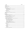
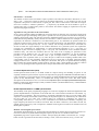
nmrPipe. The role of the mddNMR is to replenish complete data matrix with reconstructed points (Fig. 1).
The software offers three general possibilities (i) direct Fourier transform, all missing points are set to zero;
(ii) multi-dimensional decomposition (MDD); and (iii) compressed sensing (CS).
In this manual, usage of the software is described by several commented examples. In addition,
complete set of parameters and formats of essential files are given in Appendixes. Description of underlying
mathematical algorithms and processing protocols can be found in our papers listed above, and references
cited therein.
NUS
full
mddNMR
Figure 1. The software replenishes time domain data points in the indirect dimensions that are missing in the
NUS set and produces the full data set amenable for regular Fourier transform
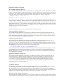
qMDD graphical user interface
The primary mode of mddnmr usage, which gives access to the full set of the software functionalities, is by
C-shell scripts. There is, however, a graphical user interface (GUI) that simplifies work with the program,
and is especially recommended for beginners. It is started with command
qMDD
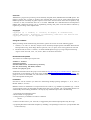
A window is opened,
which invites to select a spectrum for processing. For example, you may select ubi_ghn_co_S_nls.fid, which
is one of the example experiments in http://pc8.nmr.gu.se/~mdd/Downloads/mdd_examples/ (data type is
recognized by directory name, e.g. .fid for Variant/Agilent). Directory named ubi_ghn_co_S_nls.proc is
created, which is the place to find all files discussed below. Answer “yes” for the question (if any) about
overwriting existing processing files. You are ready to process the spectrum by pressing button “RUN”.
A new terminal window opens (not shown), in which script proc.sh is executed. When the script is
successfully finished, look at the resulting spectrum in nmrDraw by pressing “Open nmrDraw” or starting
nmrDraw in a terminal window. Look at three projections of the 3D spectrum stored in H1.C13.dat,
1H.N15.dat and N15.C13.dat or the 3D spectrum located in directory ft . From the figure above, you may
notice that the calculations have been performed with “FT” mode, which is the fastest and most robust
method, albeit it provides the poorest results due to massive aliasing artefacts. Nevertheless, “FT” mode is
useful since it allows fast look at the spectrum and adjustment of nmrPipe processing parameters (e.g.
phases).
MDD calculation
MDD processing is activated by selecting “MDD” checkbox. Prior to pressing “RUN”, you may define a
small region of interest by setting “First point ppm” and “Region of Interest SW” (with “First point” as its
downfield border) in ppms followed by pressing “Save” button. This reduces the calculation time
proportionally to the region size. Check also parameter “# threads”, which specify how many computational
tasks can run simultaneously on your computer. For modern computers, the number is 2-8 depending on how
many processors and cores are available.
Press “RUN” button and wait until output in the terminal window indicates successful completion of the
calculations. Look at the spectrum in nmrDraw. The GUI allows modification of several most important
parameters and C-shell scripts. This is done in the “Advanced” display. For example, you may set parameters
CT_SP and CEXP to “nyn” in order to activate R-MDD mode for the 2nd indirect dimension (N15) of the
experiment. You need to press “save” to activate the changes. Three scripts proc.sh, fidSP.com and
recFT.com can be edited by pressing corresponding buttons. Meaning of these files and parameters is
described in the next section.
Adjusting conventional processing parameters
mddNMR software uses nmrPipe for spectral data conversion and traditional processing. There are two
scripts that deal with these: fidSP.com and recFT.com. The former is responsible for conversion of the
spectrum to the nmrPipe format and processing of the directly detected dimension. The latter processes all
indirect spectral dimensions after the missing data in the time domain interferogram is replenished by
mddNMR. The scripts can be viewed and edited from “Advanced” display by pressing the corresponding
buttons. The procedure can be illustrated on gNhsqc_S.fid spectrum example. Load the spectrum using
“Browse” button and answer “Yes” to the question (if any) to discard the existing processing scripts. Process
the spectrum with “FT”. Disregard an error massage (if any) in the terminal window after the line “test.dat
ready”. Inspection of the spectrum in nmrDraw shows that phase in the directly detected dimension requires
adjustment by ca. 70 degrees. Press “fidSP.com” button in the “Advanced” display and set the phase
correction as shown below (in the highlighted line). Save the script and rerun the calculations.
var2pipe -in fid -noaswap -aqORD 0 \
-xN
2048
-yN
192
-xT
1024
-yT
96
-xMODE
Complex
-yMODE
Rance-Kay
-xSW
13008.100
-ySW
2600.300
-xOBS
800.128
-yOBS
81.085
-xCAR
4.755
-yCAR
116.641
-xP0
156.1
-yP0
0.0
-xP1
0.0
-yP1
0.0
-xLAB
H1
-yLAB
N15
-ndim 2
-aq2D States \
| nmrPipe -fn SOL
| nmrPipe -fn SP -off 0.450 -end 0.970 -pow 2 -c 0.500
| nmrPipe -fn ZF -auto
| nmrPipe -fn FT -auto
| nmrPipe -fn PS -hdr
| nmrPipe -fn PS -p0 70 -p1 0 -di
| nmrPipe -fn EXT -x1 11ppm -xn 5ppm -sw -round 16
| pipe2xyz -z -out ft/data%03d.DAT -ov -nofs -verb
\
\
\
\
\
\
\
\
\
\
\
\
\
\
\
\
Compressed Sensing
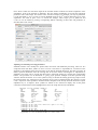
CS processing is activated by selecting “CS” checkbox. You may try CS on gNhsqc_S.fid spectrum example.
Note that in mddNMR version 2.0, CS can be used only for 2D and 3D spectra. First, process the spectrum
with “FT”. Adjust the phase for the directly detect dimension as described in the previous section. Check the
CS box and press “RUN” to calculate the spectrum. The result, which is stored in test.dat file, can be viewed
in nmrDraw. “Advanced” view (see figure below) allows checking and editing the essential parameters for
CS. For example, one can chose to use Iterative Reweighted Least Squares (IRLS) or Iterative Soft
Thresholding (IST) algorithms. Meanings and recommended values for the parameters are indicated in
contextual help, which appears when the mouse cursor is placed on the parameter field.
Master script proc.sh
The role of GUI qMDD is to collect and check input from the user and to produce all necessary files for the
calculations. The actual calculations are performed by C shell script called proc.sh (or alike). The GUI
supports only basic and most frequently used features of the software, while more advanced processing may
require editing of the master script. The script can be viewed and modified in “Advanced” view by pressing
button proc.sh or in any text editor. As soon as the script is ready, it can be run in a terminal window. For
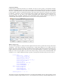
example, proc.sh script for MDD processing of gNhsqc_S.fid spectrum described in the previous section is
#!/bin/csh
setenv FID ../gNhsqc_S
setenv fidSP fidSP.com
setenv REC2FT recFT.com
setenv in_file nls.in
setenv selection_file nls.hdr_3
setenv FST_PNT_PPM 11
setenv ROISW 5
setenv proc_out test.dat
setenv METHOD MDD
setenv MDDTHREADS
2
#MDD related parameters
setenv NCOMP 25
setenv NITER 50
setenv MDD_NOISE
0.7
setenv lambda 0.01
mddnmr4pipeN.sh
1 2 3 4 5
The master script sets all parameters that have to be altered from defaults. This is done by setting C-shell
environment variables using command sentenv . The calculations are started by command mddnmr4pipeN.sh
at the end of the script. As arguments, the command takes list of tasks to be done, which are defined by
unique numbers (see next section).
Advanced processing
The most general mode of operation for mddnmr software is by using command line input. Several examples
presented in this manual illustrate most of the software features. The commands are typically arranged into
short C-shell (Unix) scripts. The master script, which is called proc.sh in this manual and in all examples,
first sets several parameters (most of the parameters have good defaults values, and are not set explicitly).
The parameters are set as Unix environment variables with command setenv (see examples). They can be
changed by modifying the script. Finally the processing is performed by mddnmr4pipeN.sh command. As
line parameters mddnmr4pipeN.sh takes a list of steps, which are integer numbers. Typically steps 1 - 5 are
executed sequentially because output from a previous step serves as an input for the next one. The steps are:
0
1
2
3
4
5
42
– print full list of parameters recognized by the program.
– conversion of ser/fid to nmrPipe format; processing of the direct dimension and extraction of
region of interest (ROI) (see parameter fidSP).
– preparing input for MDD calculations.
– MDD calculations over all sub-regions of the ROI.
– full reconstruction is produced from MDD components and residuals (see MDD_NOISE).
– the full time domain reconstruction obtained in step 4 is processed using an nmrPipe script (see
parameter REC2FT)
– MDD shapes obtained on step 3 are processed by nmrPipe and written into Unified Spectral
Format (USF3) (see parameters Proc3D_* and Proc4D_*).
Several steps can be executed in one line, e.g.
mddnmr4pipeN.sh 1 2 3 4 5
or can be done by consecutive calls of mddnmr4pipeN.sh, for example:
mddnmr4pipeN.sh 1 2 3
mddnmr4pipeN.sh 4 5
In the first case, the program passes the data from one step to another in memory. In the latter mode,
intermediate results are stored in files in working directory MDD.
Input files
There is at least one file, which needs to be prepared for the processing. Name of this file is conveyed to
mddNMR by parameter fidSP. The file is an nmrPipe script that performs conversion from spectrometer to
nmrPipe data formats using programs bruk2pipe or var2pipe, Fourier transform of the directly detected
dimension and storing of region of interest (ROI) to disk. In this manual and in all examples, the script is
called fidSP.com. The script can be produced by command nus2pipe from mddNMR software or can be
prepared by editing the data conversion script produced by programs bruker/varian from nmrPipe package.
For example, for experiment 57 from the examples, correct fidSP.com file is produced by
nus2pipe -f 57 -t Bruker
Below is an example of the fidSP file for experiment 57.
bruk2pipe -in ./ser -bad 0.0 -aswap -DMX -decim 2000
-dspfvs 20 -grpdly 67.9862518310547
-xN
2048
-yN
1
-zN
3712
-xT
1024
-yT
0
-zT
856
-xMODE DQD
-yMODE Complex -zMODE Complex
-xSW
10000.000 -ySW
2500.000 -zSW
2500.000
-xOBS
600.130 -yOBS
150.903 -zOBS
60.811
-xCAR
4.702 -yCAR
175.327 -zCAR
115.840
-xP0
-46.9
-yP0
0.0
-zP0
0.0
-xP1
22.4
-yP1
0.0
-zP1
0.0
-xLAB
1H
-yLAB
13C
-zLAB
15N
-ndim 3 -aq2D States \
| nmrPipe -fn POLY -time
\
| nmrPipe -fn SP -off 0.450 -end 0.970 -pow 2 -c 0.500 \
\
\
\
\
\
\
\
\
\
\
\
|
|
|
|
|
|
nmrPipe -fn
nmrPipe -fn
nmrPipe -fn
nmrPipe -fn
nmrPipe -fn
pipe2xyz -z
ZF -auto
FT -auto
PS -hdr
PS -p0 0 -p1 0 -di
EXT -x1 11ppm -xn 5ppm -sw -round 16
-out ft/data%03d.DAT -ov -nofs -verb
\
\
\
\
\
Script fidSP.com may be modified, for instance, for adjusting phase in the indirect dimension or chemical
shift references. On step 1, script fidSP.com is used as a template for generating several scripts (FTx.sh*) ,
which are actually used in the processing.
Name of another important nmrPipe script is set by parameter REC2FT. This is an nmrPipe script that
performs regular processing of the full reconstructed spectrum in all indirect dimensions. User may need to
change some parameters, e.g. phase corrections, weighting functions, linear prediction, etc. To do this, make
and/or edit a local copy of the script recFT.com, which is located in the ${MDD_NMR}/com directory.
Processing parameters
The parameters are typically set in the master C-shell script using command setenv. Full list of parameters
with their current values can be viewed by command
mddnmr4pipeN.sh 0
Since most of the parameters have good default values and typically only few parameters need to set
explicitly. For an illustration, let us look at the commented master script for processing scripts for experiment
57, which is one of the examples provided with the software. The experiment is a 3D HNCO spectrum
recorded on Bruker spectrometer using NUS acquisition mode in TopSpin 3.0.
# input/output files
setenv FID ../57
# location of directory with the experiment
setenv fidSP fidSP.com
# script for conversion to nmrPipe
setenv in_file nls.in
# parameters of the NUS schedule
setenv selection_file nls.hdr_3 # nus schedule
setenv REC2FT recFT.com
# pipe procession of the indirect dimensions
setenv proc_out ft/test%03d.dat # nmrPipe template for the final spectrum
# Definition of a small region of interest (ROI) in the direct dimension
setenv FST_PNT_PPM 8 # first point in ppm
setenv ROISW 0.5
# ROI size in ppm
#MDD related parameters
setenv MDDTHREADS 2
#
setenv NCOMP
25
#
setenv NITER
100
#
setenv SRSIZE
0.1
#
setenv MDD_NOISE 0.7 #
setenv lambda
0.01 #
setenv CT_SP
nnn
#
setenv CEXP
nnn
#
maximal number of parallel processes
number of components per sub-region
number of iterations
approximate size of sub-region in ppm
factor for adding residuals to the MDD reconstruction
MDD lambda
parameter CT_SP in file nls.in is overridden
parameter CEXP in file nls.in is overridden
# start actual calculations
mddnmr4pipeN.sh 1 2 3 4 5
In the script above, only first four parameters, which that are typed in bold, are needed to be set explicitly.
The remaining parameters are there mostly for display.
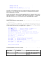
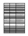
Table 1. Parameters recognized by mddNMR software.
Parameter name
Default value
CEXP
CS_alg
IRLS
Meaning and references for examples
If set, override value in nls.in file
CS algorithm: IRLS – iterative reweighted
least squares, or IST – iterative soft
thresholding
CS_lambda
1.0
CS_niter
10
CS_norm
CS_ZF
0
2
CT_SP
DATAMAP_FILE
DIM_MERGE
f180
FID
FIX_FREQ
FIX_FREQ_FILE
FST_PNT_PPM
10
ft4
FT4DX
FTX_2D
FTXTREC
in_file
./XYZA/ft4.xyza
FTx.sh
./XYZA/ft4sp.xyza.2D
./XYZA/ft4trec.xyza
lambda
0.005
MAP_FACTOR
MDD_DIR
MDD_FILE
MDD_NMR
MDD_NMR_COM
MDD_NOISE
1
./MDD
./MDD/region
…./mddnmr1.8
…./mddnmr1.8/com
0.85
MDD_STDERR
stderr
MDD_STDOUT
stdout
MDD_WORK_DIR
MDDRUNS
MDDTHREADS
.
./regions
2
METHOD
NCOMP
FT
30
ndim
NI
NIMAX
NIMIN
NITER
NLSpoints
NUS_POINTS
NUS_TABLE_ORDER
OVLP
phase
PHASE_ORDER
300
0
3
CS regularization (default is ok for all
studied cases)
Number of iterarations for CS (default is ok
for IRLS). Change to 100-10000 for IST.
Norm for CS IRLS algorithm: 0 - 1
Frequency domain “over-digitization” in CS
algorithm (best results for 2)
If defined, dimensions to merge. Used, e.g.
to process 4D spectrum with 3D MDD
If set, overrides value in nls.in file
Directory with experimental data
Reserved
reserved
Start (downfield) of the region of interest
(ppm) in the directly detected dimension
Reserved
Reserved
Reserved
Reserved
Name and location of NUS parameter file.
By default, name is obtained from the
selection_file by changing the file extension
Tikhonov regularization for MDD: 0.0010.1 with lower value for high S/N
Reserved
Reserved
Reserved
Location of the software directory
A factor that scales residuals of the MDD
calculations as they are added to the
reconstructed spectrum: 0 - 1
If set to a file name, all error terminal
messages are redirected to the file
If set to a file name, all terminal messages
are redirected to the file
Processing working directory
reserved
Maximal number of threads, i.e. number of
processes that can be run on your computer
at the same time. The parameter relates to
number of processors and cores on the
computer.
Processing method: FT, MDD, CS
Number of MDD components per subregion.
If set, override value in nls.in file
If set, override value in nls.in file
If set, override value in nls.in file
If set, override value in nls.in file
Number of iteration for MDD calculations
reserved
reserved
reserved
Overlap between sub-regions in points
If set, override value in nls.in file
If set, reshuffle FID’s inside each hyper-
Proc3D_X
Proc3D_Y
shapeProc3D_%c.sh
shapeProc3D_Y.sh
Proc3D_Z
shapeProc3D_Z.sh
Proc4D_A
shapeProc4D_A.sh
Proc4D_YZ
shapeProc4D_YZ.sh
proc_out
./ft/tdrec%03d.dat
REC2FT
recFT.com
RECHEAD
ROISW
./XYZA/ft4sp.xyza
6
RUNQUE
seed
selection_file
2345
SHAPEMAP
SHAPEMAP_FILE
./MDD/regionMAP
soft_mode
SPARSE
SpecParFile
SRSIZE
SW
XDimSize
p
./XYZA/_t.hdr
0.18
1
complex point, e.g. setting ‘1 3 2 4’ results
in swapping of the 2nd and 3rd FID’s. The
parameter is analogous to -aqORD flag in
nmrPipe, which does not work for NUS
processing. See also programs fid_shuffle
and ser_shuffle .
reserved
Script for processing MDD shapes for Y
dimension
Script for processing MDD shapes for Z
dimension
Script for processing MDD shapes for A
dimension
Script for processing MDD merged shapes
for YZ dimensions in a 4D spectrum
nmrPipe template for the final output
spectrum
Script to process indirect dimensions in a
3D spectrum
reserved
Size of the region of interest in the directly
detected dimension, ppm
reserved
Random seed for MDD calculations
NUS schedule file, typically comes with the
experiment
Co-processing: setting correspondence of
dimensions between two experiments
Co-processing: file with the reference MDD
shapes
reserved
If set, overrides value in nls.in file
reserved
Approximate size of sub-region in ppm
If set, overrides value in nls.in file
reserved
The MDD solver has one parameter that mostly affects quality of the solution, namely, number of
components (parameter NCOMP) per sub-region. Guidelines on correct setting for the parameter can be
found in our papers. In most cases, however, a default value of ca 30 for a sub-region strip of 0.1-0.2 ppm
(parameter SRSIZE) in the directly detected 1H dimension is a good guess. In short, the number of
components must be 20-50% larger then number of expected cross-peaks for 2D’s and triple resonance
backbone experiments, or number of diagonal peaks for 3-4D NOESY/TOCSY experiments. Note that
number of components refers to a sub-region. NCOMP value must be sufficient for a sub-region with
maximal expected number of peaks.
MDD shapes
The MDD model looks for an approximation of a M-dimensional spectral matrix by the sum of a
small number of tensor products of one-dimensional vectors:
SMDD = Σβ βa βF1 ⊗ … βFM-1 ⊗ βFM
(1)
where the model spectrum SMDD is the sum of fixed number of components Nc enumerated by index
β=1…Nc. Each component is given by the product of normalized vectors βFm for every spectral dimension
m=1…M, referred to below as shapes, and the component amplitude βa. The term shape is introduced here in
relation to the spectral line shape; its several synonyms are present in the literature, i.e. loads, modes, factors,
etc. Symbol ⊗ denotes the outer product operation, which produces M-dimensional matrix from M onedimensional shapes.
A simple approach is to think about a component as the representation of a cross peak in a multidimensional spectrum. The shapes then are traditional line-shapes of the peak in all dimensions. The actual
situation, however, is more complex, since the components do not always have a one-to-one correspondence
to peaks. In general, a peak showing complex structure, e.g. in an E.COSY spectrum, may require several
components for its description. It also can be the other way around, as in 3D NOESY spectrum - one
component may accommodate several cross peaks. It is important to emphasize that the MDD model does
not make any assumptions about the shape vectors β Fm. Thus it can be equally well applied to data in the time
or frequency domains, as well as combination of both.
The reconstructed spectra are produced by summation over all components (Eq. 1). Thus typically,
dealing with the individual components is not needed. However, the shapes can be stored in both time and
frequency domains.
# Storing MDD shapes using step 42
mddnmr4pipeN.sh 1 2 3 42
Upon completion of step 42, two files in XML format (see also USF3 format) are produced, which contain
shapes in frequency and time domain. The shapes are also stored in nmrPipe format in directory SHAPES
and can be viewed using nmrDraw. For example, columns in file SHAPES/sh_Y_03.dat contain the
processed shapes for first indirect dimension from the 3rd sub-region of the spectrum.
Parallel calculation for faster MDD and CS processing
MDD and CS calculations may be lengthy. The computation time rapidly increases with amount of
experimental data, number of iterations, number of components (for MDD), and size of the final spectrum
(for CS). Calculations for different sub-regions are independent and can be performed in parallel on several
CPUs that are available on one computer or within a local network. On one computer, parallel calculations
are organized simply by setting parameter MDDTHREADS to the number of CPUs. In order to distribute
calculations over a network, e.g. for a Linux cluster, step 3 is performed off-line. First steps 1 and 2 are
performed.
# Preparing input for sub-regions
mddnmr4pipeN.sh 1 2
This produces files regions.runs and MDD/regionXX.mdd, which is the only input for standalone MDD and
CS solvers, mddsolver and cssolver, respectively. File regions.runs is a C-shell script. Each line in it contains
a command for running calculations for one region. The commands may run in parallel on one computer or
be distributed over the network together with MDD/regionXX.mdd for corresponding regions. When
calculations are complete, the results, which are files MDD/regionXX.res or MDD/regionXX.cs, need to be
collected to the original MDD directory followed by the spectrum reconstruction and final nmrPipe
processing (steps 4 and 5).
# time domain spectrum reconstruction and final nmrPipe processing
mddnmr4pipeN.sh 4 5
GUI qMDD provides a simple possibility to distribute calculations using password-free ssh access and shared
file system. If box “Send computations to remote host” in GUI is checked, the following lines are added to
the master script proc.sh .
mddnmr4pipeN.sh 1 2
ssh login@host "mkdir -p tmpxxx/"
scp -C -r MDD regions.runs login@host:~/tmpxxx/
ssh login@host "cd tmpxxx/; queMM.sh regions.runs"
scp login@host:"~/tmpxxx/MDD/*.[rc]*" MDD/
mddnmr4pipeN.sh
4 5
The procedure runs script queMM.sh (part of mddNMR package) on a remote host, which distributes
calculations over specified set of computers in the network. If the master script is ran from a directory, which
is shared with other nodes in the network, ssh is not needed and the lines above are simplified to:
mddnmr4pipeN.sh 1 2
queMM.sh regions.runs
mddnmr4pipeN.sh 4 5
Note that the header of queMM.sh should be edited for every new network.
Examples
Examples, can be downloaded from http://pc8.nmr.gu.se/~mdd/Downloads and are described in the
Appendix. For each example there is a compressed tar archive with two directories containing the spectrum
and the script[s] for its processing (*.proc). For large data sets, the spectrum may be in a separate tar archive,
which allows skipping download of large examples data files.
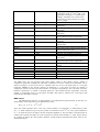
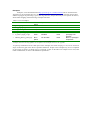
Table 1. List of examples:
File name
1
2
4
4
5
6
gNhsqc_S.tgz
ubi_ghn_co_S.tgz
284_hncoca.tgz
57.tgz
BPgnoesyNhsqc_S.tgz
az_HNCA_high_res.tgz
7
HD384_plasma_gChsqc.tgz
Protein &
citation
Azurin
Ubiquitin
Ubiquitin
Ubiquitin
Azurin 1
Blood
plasma
Experiment
Spectrometer
comment
2D HSQC
3D HNCO
3D HNcoCA
3D HNCO
3D 15N NOESY-HSQC
3D HNCA
Varian
Varian
Bruker
Bruker
Varian
Varian
BioPack
BioPack
2D 13C HSQC
Varian
BioPack
sparsifying of full
spectrum*
BioPack, sparsifyingof
full spectrum*
(1) Jaravine, V.; Ibraghimov, I.; Orekhov, V. Y. Nature Methods 2006, 3, 605.
*examples cannot be ran using qMDD, see description in the Examples section in the Appendix
To speed up calculations and save disk space in the examples, the master scripts (proc.sh) are set for narrow
strips of about 0.2 ppm in the direct acquisition dimension. Scripts in the examples may serve as templates
for processing of spectra of similar type. For example, scripts for the HNcoCA example can be used, after
minor modifications, for most of the backbone experiments.
APPENDIX
I. NUS schedule
NUS schedule is typically produced by spectrometer software and is saved together with the experiment. The
schedule can be also produced by running program nussampler from terminal command line:
nussampler nls.in
nussampler takes parameters from the input file nls.in (this name is used for most cases), generates a
sampling scheme and writes it to file nls.hdr_3. Both files nls.in and nls.hdr_3 are needed for processing and
must be stored together usually in the directory with fid or ser files . Typically the nls.in file is produced by
executing the script from a GUI in spectrometer software, e.g. BioPack (Varian). Alternatively, the nls.in text
file can be edited manually, and the above command for generating of a schedule can be typed from Unix
command line.
File nls.in – setting NUS parameters
Each line of NUS parameter file nls.in start with a keyword followed by a list of parameters values. All the
keywords are mandatory, but the lines order is not important. Below and in Appendix 2. several examples of
input files are explained; location of nls.in file needs to be specified by parameter in_file in the master script
(proc.sh).
___
file
NDIM
seed
SPARSE
sptype
f180
CT_SP
CEXP
NIMAX
NIMIN
NI
SW
T2
Jsp
phase
____
NDIM –
seed –
NLS_setup3d.in
3
54321
n
shuffle
nnn
nyn
yyn
40 30 1
0 0 0
7 30 1
1824.818 2112.825
1.0 0.05 1
0 0 0
0 0 0
8389.262
number of dimensions, e.g. 3 for 3D spectrum
seed for random number generator. If seed and other parameters are not changed output NUS
schedule table will be the same on the same computer architecture.
SPARSE – y|n - during the processing, the flag toggles processing of a real sparse spectrum (‘y’) vs sparsifying
of a full spectrum (‘n’). When setting up a BioPack experiment on a spectrometer, it toggles between
NUS and regular sampling.
f180 –
flags to specify 180 degree linear phase. Set y or n for every dimension. Direct dimension is the last
one. The flag is important only for dimensions with CT_SP equal ‘y’.
CEXP – y|n toggle R-MDD / MDD mode for a dimension, with ‘y’ time domain shape in the dimension is
expected to be autoregressive. In other words, we assume that the FID in the dimension is a complex
exponent. CEXP=y may be used, for example, for HNCO and HNcoCA experiments, but not for the
NOESY’s.
CT_SP - n|y toggles mirror image processing for dimensions with CEXP=’y’ . Set ‘n’ for the first indirect
dimension. CT_SP have to be stet to ‘y’ for the constant-time second indirect dimension (typically
15N) in the triple resonance experiments.
NIMAX – full indirect sizes of the spectrum (you may put 1 for the (last) direct dimension)
NI Multiplication of all NI values gives total number of (hyper-complex) points in the indirect dimensions.
Put 1 for the direct dimension, which is the last number.
SW –
spectral windows for dimensions in Hz
T2 –
estimate of transverse relaxation times for each dimension for NUS. Use large value for dimension
with constant-time (CT) evolution
Jsp –
estimated resolved J-coupling for each dimension
phase –
zero order phase correction for indirect dimensions. Used for dimensions with CT_SP=y
File nls.hdr.3 – NUS table
The number of entries in the NUS table is equal to product of NI values for all indirect dimensions, i.e. NI x
NI2 [ x NI3 ...]. Each line consists of indexes for all indirect dimensions, i.e. two numbers per line for 3D
experiment. The points are selected from a regular grid, thus values of the indexes in the table are integers
from zero to NImax-1, NI2max-1,[NI3max-1 ...], respectively. By default, the NUS schedule is given in
random order, that is evolution time points are not ordered. This allows stopping an experiment at any time
without losing digital resolution.
Algorithm for the generation of the NUS schedule
NUS or sparse schedule suitable for MDD/CS processing selects for detection only a fraction of points from
a complete Nyquist grid. Sampling on the grid is a special case of more general NUS that allows sampling at
arbitrary selected time points. The selection of points in mddNMR software (see nussanpler) is governed by a
multi-dimensional probability density function for all indirect evolution dimensions. For example for a 3D
experiment, the function is defined on a two-dimensional grid (t1, t2) determined by spectral widths and
maximal acquisition times (t1max, t2max) in the two indirect dimensions. The distribution is obtained as a
product of the two envelopes, P(t1,t2) = P1(t1) x P2(t2). The envelope functions P1(t1) and P2(t2) are
devised to match the signal intensity in the indirect dimensions for a particular system and experiment.
Currently two possibilities are implemented: (i) mono-exponential relaxation- P (t1) = exp(-t/T2); (ii)
modulation by the one-bond J-coupling- P(t2) = cos(t pi/J). The J-modulation can be combined with the
relaxation decay. The transverse relaxation time T2 and value of the J-coupling are parameters of the
procedure and are defined in the “.in” file. For a given probability distribution, we use the following
procedure to generate the NUS schedules. First, a pair of integer indices is randomly selected that
corresponds to the acquisition times (t1, t2). Then the pair is added to the sampling schedule table if the
corresponding value of the probability distribution P(t1,t2) is larger than a randomly generated number
ranging between 0 and 1; otherwise, the index pair is discarded. This process is repeated until the sampling
table contains the requested number of data points for each step. Thus, a NUS schedule is a table of evolution
delays (t1, t2) spanning maximal acquisition times and spectral widths in the indirect dimensions.
II. Unified Spectral Format (usf3)
Unified spectral format (USF3) is an XML format for compact storage and handling of spectra. It was
originally intended to present results of spectra decomposition by programs MddNMR and PRODECOMP; it
is also suggested as a general frame for compact storing of regular multidimensional and hyper-dimensional
spectra of any dimensionality. USF3 is a standard data storage format for CCPN. The latest formal
description of the format (2011-05-13) can be found at http://www.ccpn.ac.uk/ccpn/projects/extendnmr/shape-dataformat or requests from Rasmus Fogh (CCPN), Vladislav Orekhov (Swedish NMR Center), or Martin Billeter
(University of Gothenburg).
III NUS Implementations on NMR spectrometers
The flexibility of the pulse programming languages of VnmrJ and TopSpin has allowed straightforward and
generic implementations of acquisition of NUS nD data. See vendor software manuals for exact details, e.g.
documentation on BioPack. The NUS scheme is generically applicable for most if not all existing pulse
sequences. Uniformly incremented evolution delays in the pulse sequence are substituted by the values from
the NUS table for every FID. New evolution delays are produced by multiplying the indexes by
corresponding dwell time (i.e. 1/sw). For every combination of evolution times all FID’s comprising one
hyper-complex point must be recorded as one block. Thus, the block contains 2,4, and 8 FID’s for 2D, 3D,
and 4D spectra respectively. This corresponds to standard Varian/Agilent convention, but is different for old
Bruker pulse sequences.
BioPack: Varian/Agilent spectrometer
The BioPack implementation (see Varian/Agilent documentation for details) features automatic creation of a
new NUS version of any multi-dimensional pulse sequence by the use of a checkbox button in the
DigitalFilter page in the Acquire Folder of VnmrJ. After specifying the number of increments, etc., a single
button is used to generate all the NUS files, including *.in file, table of increments (*hdr_3) via the "Set
Sampling Schedule" button in the same page. Acquisition is performed in the normal manner. Saving of the
data using the BioPack macro "BPsvf" also saves the NUS files and a script to permit easy processing by the
MDD software.
NUS version of any experiment can be produced using macro BP_NLSinit(<dims>), where <dims> stands
for the number of dimensions in the experiment, thus for HNCO in the command line type
BP_NLSinit(3)
The macro prepares NUS version of the pulse sequence (look at ghn_co_S.c) and adds few additional
parameters, which can be viewed in the “text output” tab using command dgnls. Set SPARSE=’n’ ,
phase=1,2 , phase2=1,2 and use parameters nt, ni, ni2 and command time to adjust time of the experiment.
Note that parameters ni, and ni2 define only total duration of the NUS experiment, the size of the sampling
grid is defined by parameters nimax and ni2max. Set SPARSE=’y’ and calculate the sampling schedule by
using macro
BP_NLSset
The macro creates two files in the experiment directory ~/vnmrsys/expXX : nls.in and nls.hdr_3. The former
contains parameters that are used for the generating the NUS schedule
nls.in
file /home/bcbp/vnmrsys/exp4/nls
NDIM 3
SPARSE y
seed 4321
sptype shuffle
nholes 0
f180 nnn
CT_SP nyn
CEXP yyn
NIMAX 50 50 1
NIMIN 0 0 0
NI 5 50 1
SW 2500 3000 10000
T2 0.02 1 1
Jsp 0 0 0
File nls.hdr_3 contains the sampling schedule, i.e. the list of selected points from the 2D grid (13C, 15N).
nls.hdr_3
36 45
11 47
3 26
9 44
8 38
5 4
…
Files nls.in and nls.hdr_3 are needed to run and process the experiment.
TopSpin: Bruker spectrometer
Consult the user manual for TopSpin 3.0 and later versions.
IV. Examples of MDD/CS processing of spectra recorded with NUS
The examples include: (i) spectra with relatively small number of signals (up to 100-300) and limited
dynamic range (up to ca 100), examples are 2D 13C HSQC, 3D HNcoCA and HNCO; (ii) spectra of
NOESY-HSQC or TOCSY-HSQC type. Notably, requirements for number of signals and dynamic range for
these spectra refer to diagonal signals, but not the cross-peaks. The peaks, which share line shape with
diagonal signals, may be close to the noise level.
Example of backbone experiment
2D 15N HSQC (ubiquitin, BioPack)
This example illustrates MDD and CS processing of a 2D spectrum. Extract files from tar archive
gNhsqc_S_30Jun2011.tgz.tgz and change directory to gNhsqc_S/gNhsqc_S.proc. Run master script proc.sh
and look at the resulting spectrum using nmrDraw. Phase in the directly detected dimension requires
correction, which can be done by changing one number in file fidSP.com . Namely, change line
| nmrPipe -fn PS -p0 0 -p1 0 -di
\
to
| nmrPipe -fn PS -p0 70 -p1 0 -di
\
and rerun proc.sh script. Open proc.sh in a text editor and change parameter METHOD to MDD or CS in
order to compare results for different methods. To shorten the calculations you may reduce the region of
interest in ppm’s by changing parameters FST_PNT_PPM and ROISW. The spectrum has been recorded
with random NUS 38%, i.e. 96 points were recorded out of 256. You may check how quality of the spectrum
degrades as fewer data points are used for calculations. For this, set parameter NI in pros.sh to a value
smaller than 96, e.g. for 25% NUS add line
setenv NI 64 1
By setting variable NI in proc.sh we override the values stored in file nls.in.
3D HNCO (ubiquitin, TopSpin 3.0)
This example illustrate MDD and CS processing of a 3D triple-resonance spectrum. Extract files from tar
archive 57hnco_30Jun2011.tgz and change directory to 57hnco /57.proc. Run the master script proc.sh and
check the resulting spectrum in nmrDraw. The spectrum was recorded with 25% NUS. Results for less data
can be checked as described in the HSQC example above.
3D HNCO (ubiquitin, BioPack)
This example illustrate MDD and CS processing of a 3D triple-resonance spectrum. Extract files from tar
archive ubi_ghn_co_S_nls_30Jun2011.tgz and change directory to ubi_ghn_co_S_nls
/ubi_ghn_co_S_nls.proc. Run the master script proc.sh and check the resulting spectrum in directory ft and
2D projections in 1H.C13.dat N15.1H.dat N15.C13.dat . The spectrum was recorded with 6% NUS. Note the
fid reshuffling from phase2,phase to phase,phase2 in the master script:
if( ! -f fid ) fid_shuffle ../ubi_ghn_co_S_nls.fid/fid fid 4 1 3 2 4
Since processing of the directly detected dimension is performed by nmrPipe in 2D mode (script FTx.sh.2D),
this reshuffling cannot be performed by var2pipe. It cannot be done either by setting mddNMR parameter
PHASE_ORDER to 1 3 2 4, because decoding of the Echo-Anti-Echo has to be performed by nmrPipe prior
to the processing by mddNMR.
3D HNcoCA (ubiquitin, TopSpin 3.0)
This example illustrate MDD and CS processing of a 3D triple-resonance spectrum. Extract files from tar
archive 284_hncoca_30Jun2011.tgz and change directory to 284_hncoca/284.proc. Run the master script
proc.sh and check the resulting spectrum in directory ft, file 284.tf3 and 2D projections in 1H.C13.da,t
N15.1H.dat, N15.C13.dat . The spectrum was recorded with 9% NUS. Note that scripts fidSP.com and
recFT.com have been adjusted relative to the setting provided by GUI qMDD. Thus, phase in the directly
detected dimension is corrected in fidSP.com.
3D NOESY (BioPack)
This example shows processing of 3D 15N NOESY-HSQC spectrum of a 15 kDa protein. Extract files from
tar archive BP_gnoesyNhsqc_S_30Jun2011.tgz and change directory to BP_gnoesyNhsqc_S/
BP_gnoesyNhsqc_S.proc. The experiment has been run in SPARESE (20%) mode and saved in BioPack
using macroses BP_NLSinit, BP_NLSset, BPsvf. Run master script proc.sh and check the resulting spectrum
in directory ft, file 284.tf3 and 2D projections in 1H.C13.da,t N15.1H.dat, N15.C13.dat.
3D HNCA (azurin, BioPack, full spectrum)
This example shows MDD processing of a 3D spectrum, which was recorded in full. Thus, spectrum
reconstructed from a small fraction of data points can be compared with the full spectrum processed using
traditional DFT. A high resolution HNCA experiment, which was used for our publication Jaravine, V., et
al. Nature Methods 2006, 3, 605, was recorded for globular 14 kDa protein azurin. Extract files from tar
archive az_HNCA_high_res_30Jun2011.tgz and change directory to az_HNCA_high_res.proc. Since the
spectrum was not recorded in NUS mode, it cannot be processed using qMDD GUI. Script Proc.sh produces
NUS schedule (10%) “on the fly” by running program nussampler on nls.in file. Note that parameter
SPARSE in nls.in file is set to “n”. This tells mddNMR that sparse data are to be extracted from a full
spectrum. For spectra recorded in real NUS mode, the parameter must be set to “y”. Below you see content
of commented script Proc.sh:
#!/bin/csh
setenv FID ../az_HNCA_high_res # input experiment (without .fid )
setenv in_file nls.in
# local copy of nls.in with NUS schedule parameters
setenv selection_file nls.hdr_3 # NLS schedule file to be produced by nussampler
setenv fidSP fidSP.com # nmrPipe script for fid conversion and DFT of the direct dim
setenv REC2FT recFT.com # nmrPipe script to process reconstruction after mdd calculations
# MDD related -------------------setenv FST_PNT_PPM 8.75 # leftmost point of region of interest (ROI)
setenv ROISW 0.15
# full ROI size (ppm)
setenv SRSIZE 0.1
# recommended size of sub-region
setenv NITER 50
# number of iteration
setenv NCOMP 30
# default number of components for one sub-region
setenv lambda 0.002
# Tikhonov regularization parameter
setenv MDD_NOISE 0.2 # scales residuals as they are added to the reconstructed spectrum
setenv proc_out ft/test%03d.dat # nmrPipe template for the final 3D spectrum
#####################################################################
############### end of definitions ##################################
nussampler $in_file
# the spectrum has been recorded in full and is “sparsed”
# for processing; so calculate NUS table here
# check/edit file nls.in for the NUS schedule parameters
# process spectrum with mdd
mddnmr4pipeN.sh
1 2 3 4 5
# make 2D projections of the final 3D spectrum
proj3D.tcl -in $proc_out
## uncomment the following lines to process the full spectrum for comparison
# FTx.sh XYZA/FTx.xyza
# make FT for directly detected dim for ref
spectrum
# recFT.com XYZA/FTx.xyza ft/ref%03d.dat
# FT of Y and Z dimensions
# cd ft
# proj3D.tcl -in ref%03d.dat
# make 2D projections of reference spectrum
2D 13C HSQC (fish blood plasma, matabolomcs)
This a high resolution 2D 13C HSQC is recorded for a fish blood plasma sample in a metabolomic study by
Drs. L. Samuelsson and J. Larsson, Dept. of Physiology/Endocrinology The Sahlgrenska Academy at
Gothenburg University. The data set, which is recorded in full, can be used to illustrate quality of the
spectrum obtained using different NUS schedules. Extract files from tar archive HD384_plasma_gChsqc
_30Jun2011.tgz and change directory to HD384_plasma_gChsqc.proc . Since the spectrum was not recorded
in NUS mode, it cannot be processed using qMDD GUI. Script proc.sh produces NUS schedule “on the fly”
by running program nussampler on nls.in file. Note that parameter SPARSE in nls.in file is set to “n”. The
fully sampled spectrum is ‘sparsed’ to 15% (ni/nimax = 180/1200). Both 15% MDD sparse spectrum and
reference-full (100%) spectrum are written for comparison.
V. Tools in the package
Programs
fid_shuffle
program to shuffle (=re-order) 1D FIDs in Varian fid
Use: fid_shuffle <input fid> <output fid> <array size> <n1> <n2> ... <n arr size> }
<input fid> - data file
<array size> <n1> <n2> ... <n arr size> - size of reshufled block and new order of 1D's
Example 3D phase2,phase to phase,phase2
: <input fid> <output fid> 4 1 3 2 4
Example 4D phase3,phase2,phase to phase,phase2,phase3 : <input fid> <output fid> 8 1 5 3 7 2 6 4 8
ser_shuffle
program to shuffle (=re-order) 1D FIDs in Bruker ser
Use: ser_shuffle <input ser> <output ser> <FID size in 4 byte words> <NF -FID's in block> <n1> <n2> ... <n NF> }
change order of FID's within block; initial order is 1 2 3 4 5 6 7 ...
Example: ... 4 1 3 - only 1st and 3rd FID's out of 4 are passed to the output
Example 3D phase2,phase to phase,phase2
: ... 4 1 3 2 4
Example 4D phase3,phase2,phase to phase,phase2,phase3 : ... 8 1 5 3 7 2 6 4 8
mddsolver, cssolver
Standalone MDD and CS solvers respectively.
Shell scripts
queMM.sh
allows to do parallel calculations of step 3 on multi-CPU localhost or a network cluster (over password-free ssh); Edit
parameters in this script setup for your local network.
recFT.com
default template nmrPipe script, for processing of YZ dimensions; it is normally copied to each *.proc directory and
manually edited, e.g. to set indirect phases if different from defaults (0 0).
nussampler
NUS generator; described above
VI. Copyright and Legal Information
Copyright (C) V. Orekhov, V. Jaravine, M. Mayzel, K. Kazimierczuk, Swedish NMR Center, University of
Gothenburg, 2004-2011.
Date: Jul 3, 2011
DESCRIPTION
MddNMR is a program for processing uniformly and non-uniformly sampled (sparse) NMR spectra.
The following is legal information pertaining to the use of the MddNMR program. It applies to all MddNMR
source files, executable (binary) files, configuration and documentation files contained in the official
MddNMR archives. (Certain portions refer to custom versions of the software, there are specific rules listed
below for these versions also.) All of these are referred to here as "the software".
THIS NOTICE MUST ACCOMPANY ALL OFFICIAL OR CUSTOM MddNMR FILES. IT MAY NOT
BE REMOVED OR MODIFIED. THIS INFORMATION PERTAINS TO ALL USE OF THE PACKAGE
WORLDWIDE. THIS DOCUMENT SUPERSEDES ALL PREVIOUS LICENSES OR DISTRIBUTION
POLICIES.
IMPORTANT LEGAL INFORMATION
While the use MddNMR is essentially free of any costs for noncommercial purposes, commercial users and
software developers, who wish to bundle MddNMR with other software, will be asked for support of the
research and development of MddNMR. For commercial purposes of MddNMR please contact the copyright
holders. Permission is granted to use the MddNMR program and all associated files in this package for
making calculations. Use of the software for academic and educational purposes is free. The user retains all
rights to the results and may use them for any noncommercial purpose. The following legal information
exclusively concerns distribution and use of the software for noncommercial purposes.
When results obtained by MddNMR are used in lectures, publications or other similar occasions, then a
reference to the authors and at least one of the following papers is to be made:
(1) Orekhov, V.Y. and V.A. Jaravine, Analysis of non--uniformly sampled spectra with Multi--Dimensional
Decomposition. Prog. Nucl. Magn. Reson. Spectrosc., 2011, in press, doi:10.1016/j.pnmrs.2011.02.002
(2) Kazimierczuk, K. and V.Y. Orekhov, Accelerated NMR Spectroscopy by Using Compressed Sensing.
Angew. Chem.-Int. Edit., 2011, 123, 5670-3
This software package and all of the files in this archive are copyrighted by the authors, which are
represented by Prof. Vladislav Orekhov for distribution, copyright and other legal issues (VO). The software
may only be distributed and/or modified according to the guidelines listed below. The spirit of the guidelines
below is to provide the MddNMR package freely to as many users as possible, prevent MddNMR users and
developers from being taken advantage of, enhance the life quality of those who come in contact with
MddNMR. This legal document was created so these goals could be realized. You are legally bound to
follow these rules, but we hope you will follow them as a matter of ethics, rather than fear of litigation.
No portion of this package may be separated from the package and distributed separately other than under the
conditions specified in the guidelines below. This package may only be bundled in other software packages
with the explicit permission of the copyright holders. This package may only be posted in the Internet and/or
included in software compilations using media such as, but not limited to, floppy disk, CD-ROM, tape
backup, optical disks, hard disks, or memory cards with the explicit permission of the copyright holders.
CUSTOM VERSIONS
With a separate agreement a user may be granted the privilege to modify and compile the source for their
own use in any fashion they see fit. What you do with the software in your home or lab is your business,
however, in such cases the activity is usually limited by the agreement or defined by the collaborative
project. If the user wishes to distribute a modified version of the software, documentation or other parts of
the package (here after referred to as a "custom version") they must follow the guidelines listed below. These
guidelines have been established to promote the growth of MddNMR and prevent difficulties for users and
developers alike. Please follow them carefully for the benefit of all concerned when creating a custom
version. You may not incorporate any portion of the MddNMR source code in any software other than a
custom version of MddNMR without the explicit permission of the copyright holders. However authors who
contribute source to MddNMR may still retain all rights to use their contributed code for any purpose as
described below. The user is encouraged to send enhancements and bug fixes to the MddNMR authors, but
the authors are in no way required to utilize these enhancements or fixes. By sending material to the authors,
the contributor asserts that he owns the materials or has the right to distribute these materials. He authorizes
the MddNMR authors to use the materials any way they like. The contributor still retains rights to the
donated material, but by donating you grant equal rights to the MddNMR authors. The MddNMR authors
don't have to use the material, but if we do, you do not acquire any rights related to MddNMR. We will give
you credit if applicable.
CONDITIONS FOR DISTRIBUTION OF CUSTOM VERSIONS
The permission to distribute compiled custom version of the software may be granted in advance with
specific permission from VO. Typical conditions include but not limited to following conditions are met.
These conditions also apply to custom documentation based on our files. - Mark your version clearly on all
modified files stating this to be a modified and unofficial version. - Make all of your modifications to
MddNMR freely and publicly available. - Include clear and obvious information on how to obtain the
official MddNMR. - Include contact and support information for your version. - Include all credits and credit
screens for the official version. - Include a copy of this document. The MddNMR authors are not obligated
to provide you or your users any technical support.
GENERAL RULES FOR ALL DISTRIBUTION
All requests to acquire the software should be sent to VO, who normally distributes the software on behalf of
all co-authors. The permission to distribute this package under certain very specific conditions is granted in
advance to other persons or organizations, provided that the above and following conditions are met. The
software archives must not be renamed or re-archived using a different method without the explicit
permission of the authors. The full software package, as described in the next section, must always be
distributed. All forms of commercial and non-profit distribution are only allowed with explicit permission of
the copyright holders represented by VO. Clear reference to the copyright holders (at least to VO) must be
present in any description/synopsis of software. The copyright holders reserve the right to withdraw
distribution privileges from any group, individual, or organization for any reason.
DEFINITION OF "MddNMR PACKAGE" MddNMR is distributed as a number of archive containing
executables, installation scripts, examples, and documentation. MddNMR is officially distributed for PC
(LINUX) and Intel MAC (OS X 10.6 and later). Other systems may be added in the future. Distributors may
support different platforms but for each platform they support the full package must be distributed.
DISCLAIMER
This software is provided as is without any guarantees or warranty. Although the authors have attempted to
find and correct any bugs in the package, they are not responsible for any damage or losses of any kind
caused by the use or misuse of the package. The authors are under no obligation to provide service,
corrections, or upgrades to this package.
[End of Legal Information]