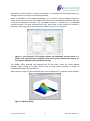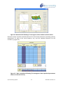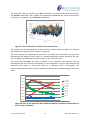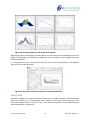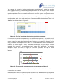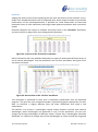
1
Global Analysis and Reaction Modeling for Kinetic Processes ReactLab TM KINETICS User Manual © Copyright Jplus Consulting Pty Ltd Jplus consulting multivariate analytical technologies ReactLab™ KINETICS Global Analysis and Reaction Modeling for Kinetic Processes USER MANUAL Contents ReactLab™ KINETICS .......................................................................................................... 1 ABOUT THIS MANUAL ............................................................................................................ 3 SYSTEM REQUIREMENTS AND INSTALLATION ....................................................................... 3 CONTACT INFORMATION AND SUPPORT .............................................................................. 3 PART 1: REFERENCE GUIDE ........................................................................................................ 4 INTRODUCTION ...................................................................................................................... 4 EXCEL TEMPLATES .................................................................................................................. 4 STARTING THE MATLAB PROGRAM ....................................................................................... 7 Program Operation ................................................................................................................ 7 Load Excel File .................................................................................................................... 7 Close Excel File ................................................................................................................... 9 Sync New Data ................................................................................................................... 9 MODEL ENTRY AND COMPILATION ....................................................................................... 9 Compile Model ................................................................................................................. 10 PARAMETER ENTRY .............................................................................................................. 11 FITTING THE MODEL TO DATA ............................................................................................. 12 Fit ..................................................................................................................................... 12 Update.............................................................................................................................. 14 Residuals .......................................................................................................................... 14 Graph GUI ........................................................................................................................ 16 SIMULATION......................................................................................................................... 17 Simulate ........................................................................................................................... 19 FACTOR ANALYSIS ................................................................................................................ 19 SVD ................................................................................................................................... 19 Jplus Consulting Pty Ltd 1 ReactLab™ Kinetics 1.1 EFA ................................................................................................................................... 20 NUMERICAL OPTIONS .......................................................................................................... 21 Restore Options ............................................................................................................... 21 QUITTING REACTLAB™ ......................................................................................................... 22 Quit .................................................................................................................................. 22 FIXED SPECTRA ..................................................................................................................... 22 AUXILIARY PARAMETERS ..................................................................................................... 22 NUMERICAL AND OTHER OPTIONS ...................................................................................... 23 HANDLING PROTONATION EQUILIBRIA, [H], [OH] and Kw .................................................. 25 MODEL ENTRY SYNTAX RULES ............................................................................................. 26 Part 2: EXAMPLES..................................................................................................................... 27 k k 2 1 B C (AtoBtoC.xlsx) ........ 27 Example 1: Consecutive Reaction Scheme A The Experiment ................................................................................................................ 27 The Data ........................................................................................................................... 27 The Model ........................................................................................................................ 28 Compilation ...................................................................................................................... 28 Initial Concentrations and Definition of Spectra ............................................................. 29 Definition of Initial Guesses for the Rate Constants ........................................................ 30 Update.............................................................................................................................. 30 Fitting ............................................................................................................................... 31 An Interesting Problem and Local Minima ...................................................................... 32 Non-Negative Spectra ...................................................................................................... 33 Residuals .......................................................................................................................... 34 Measurements at Only One Wavelength ........................................................................ 35 k k2 +1 Example 2: Enzyme Kinetics E + S ES E + P (Enz1.xlsx) ............... 35 k-1 Simulation ........................................................................................................................ 36 Stiff solver ........................................................................................................................ 39 Enzyme substrate interaction as an equilibrium ............................................................. 39 k C (AplusBtoC.xlsx).............................. 41 Example 3: Second order reaction A + B Rank deficiency, known spectra ...................................................................................... 42 Simulation as a tool for exploring rank deficient data .................................................... 43 Jplus Consulting Pty Ltd 2 ReactLab™ Kinetics 1.1 Auxiliary Parameters ........................................................................................................ 44 Example 4: Kinetics Coupled with Protonation Equilibria (Ni_ammonia_kinetics.xlsx) .... 44 Initial Concentrations in Models with Protonation Equilibria ......................................... 45 References ........................................................................................................................... 49 ABOUT THIS MANUAL This manual is in two parts. Part 1 comprises a comprehensive description of the program architecture and functionality and provides a systematic guide to using it. Part 2 consists of a series of worked examples demonstrating specific examples of analysis using pre-prepared workbooks. All these are provided in the Excel examples folder in the application installation package. They can also be downloaded independently from the web-site. Note, when they are installed in the default program files directory they are automatically assigned read-only status but can of course be copied or re-saved to a suitable working directory. SYSTEM REQUIREMENTS AND INSTALLATION Please refer to the ‘System Requirements and Installation Guide’ available on our website, and included with the ReactLab™ download. CONTACT INFORMATION AND SUPPORT [email protected] www.jplusconsulting.com Jplus Consulting Pty Ltd 8 Windsor Road East Fremantle WA 6158, Australia ABN: 83-135-664-603 Jplus Consulting Pty Ltd 3 ReactLab™ Kinetics 1.1 PART 1: REFERENCE GUIDE INTRODUCTION ReactLab™ KINETICS provides global analysis for fitting chemical reaction schemes and their parameters to multivariate spectroscopic data. It also offers extensive reaction modeling and data simulation capabilities. The program, including all algorithms and the GUI frontend has been developed in Matlab and compiled to produce the final deployable application. It requires the Matlab Component Runtime (MCR) to be installed on the same computer. This allows the program to run on computers without standard Matlab installed and is supplied as part of the installation package. All raw data, model entry and results output are organised in Excel Workbooks, which are launched from, and dynamically linked to, the ReactLab™ application. It is therefore necessary for Excel to be installed on the same computer as ReactLab™. The use of Excel provides a familiar spreadsheet format for all experimental and analysis data and results, and allows the independent application of Excel tools and features for further processing and graphical presentation. It also provides the interface for entering reaction models and all fit related parameters and numerical analysis options. When a workbook is saved it contains all information and settings associated with the current analysis session as well as the numerical data and results. This allows any number of data analyses with different model scenarios and parameter settings to be developed and saved in a self-contained format. These workbooks can be further analysed by ReactLab™ as required or reviewed independently, just using Excel. The program requires Excel analysis workbooks to retain a strict format, as is provided in the examples and templates. The process of analysing a data set using the program involves launching ReactLab™ and loading a workbook pre-populated with measurement data. Note, the workbook can be saved or reloaded at any time and will re-synchronise with ReactLab™ program according to the most recent operation. A selection of example workbooks accompanies the program in an Excel template subfolder; they are described in detail in Part 2 of this document. Note this manual describes the kinetic implementation of Jplus global analysis ReactLab™ Kinetics. A separate manual describes operation of the complementary equilibrium titration analysis application ReactLab™ Equilibria. EXCEL TEMPLATES To inspect an Excel ReactLab™ KINETICS workbook load it directly into Excel, or via the ‘Load Excel’ button in the ReactLab™ GUI. The workbook is pre-formatted containing several worksheets which provide spreadsheet formatted data and results as well as purpose designed model and parameter entry interfaces. Jplus Consulting Pty Ltd 4 ReactLab™ Kinetics 1.1 Template Worksheets: Main Data Results Sim Aux SVD About The principle model and parameter entry interface Location for experimental or simulated data Location for fitted or simulated concentration profiles and spectra Simulation parameter entry interface Used for managing known spectra Dynamically created sheet for storing SVD or EFA analysis results Sheet with contact information and the workbook format version The format of these sheets is important as ReactLab™ depends on everything being in particular locations. Figure 1 illustrates the organisation and model entry fields in the ‘Main’ worksheet which is the principle sheet of the workbook requiring user interaction. The various fields in this sheet will be described later on in this document. Figure 1: The ‘Main’ worksheet illustrating a fairly complex reaction model in coordination chemistry Important: The workbooks provided have certain areas of each sheet ‘protected’. These areas include data entry headings (generally in yellow) and certain key cells containing Excel formulas (generally in grey) used to calculate data ranges for ReactLab™. It is straightforward to unprotect any sheet using the Excel ‘unprotect’ command, but please be aware that corrupting the layout or formulae will prevent the correct interaction of the Jplus Consulting Pty Ltd 5 ReactLab™ Kinetics 1.1 spreadsheet with ReactLab™. One exception is the red coloured ‘Expand’ tabs on certain worksheets (see Figure 1). These provide an increased cell range for complex models if required. To activate these tabs first unprotect the sheet and then expand or contract the cell ranges as required. Please re-protect the sheet afterwards. It is up to the user whether to include a password for un-protection. To get a practical demonstration of ReactLab™ capabilities quickly refer to the Example workbooks and corresponding descriptions in Part 2 of this manual. What follows here is a systematic overview of the whole program. When working with new measurements start with an empty workbook template. We advise making a copy of Master_ReactLab_Kinetics_Template.xls/xlsx for this purpose. The first step is to populate the ‘Data’ worksheet with a new measurement matrix Y (dimension n_times by n_lam) as well as the corresponding wavelength and time vectors (see Figure 2). Important: when using Excel 1997-2003 compatible workbooks the maximum number of wavelengths permitted is 253 (due to the column number restriction in this version of Excel). For Excel 2007 ReactLab™ can in principle handle >17000 wavelengths (the program currently resolves 3 letter column headings = 26 3 combinations). Note therefore that saving an xlsx workbook in xls format can lead to truncation of large data sets. The time vector occupies the left hand column (C6, C7 etc.) and the wavelength vector the top row (D5, E5 etc.). The data are placed in an n_times x n_lam array for each corresponding time and wavelength coordinate. Please note that several fields in the workbook are automatically populated by Excel formulas. For example the count of the number of wavelengths and number of times at the top left (B5 and B6) of Figure 2 are evaluated by Excel from the number of time and wavelength entries. These field formulas must not be altered. They are protected (using Excel cell protection features) by default. Figure 2: Key parameters in ‘Data’ sheet. The dimensions (in grey) are calculated automatically from the data range pasted into the worksheet. Once the data is in place the workbook can be saved under a suitable name. Important: prior to ReactLab Version 1.1 Build 03 the newly populated workbook must be saved first and re-loaded into the ReactLab™ program (even if previously opened by it) in order for the new data to be recognised by the application. Jplus Consulting Pty Ltd 6 ReactLab™ Kinetics 1.1 In later versions ReactLab can be synchronised with new data in the linked workbook by pressing the ‘Sync New Data’ button in the Main GUI. STARTING THE MATLAB PROGRAM When ReactLab™ is launched it also requires the Matlab MCR to initialise. This can take a while and is very much dependant on computer performance, after which the ReactLab™ GUI appears as in Figure 3. Figure 3: Matlab GUI control panel at startup This GUI provides the main control interface for the program with a series of pushbuttons on the right hand side for key functions. These provide all the ReactLab™ program commands and their operation is described over the following pages. Note depending on the workbook status (e.g. whether a data or model are present) some of these functions may be disabled. In addition an About menu item at the top left provide details of the ReactLab™ version and licensing information. Program Operation Load Excel File Press Load Excel File in the ReactLab™ GUI to select and link to an Excel Workbook. This will launch a new instance of Excel and load the requested workbook independent of any other open Excel workbooks. Only ReactLab™ KINETICS workbook templates can be loaded. Important: Excel is launched as an ActiveX server in an independent process linked to ReactLab™ which communicates with it through its Microsoft component object model (COM) interface. The launch of Excel and ActiveX server linkage is initiated by the Matlab program. Linking to an already open workbook in Excel is NOT supported. If a workbook is prepared for analysis following the steps above it should first be saved and re-opened from the running ReactLab™ application. Note all Excel functionality is available to manipulate the Jplus Consulting Pty Ltd 7 ReactLab™ Kinetics 1.1 workbook as normal while it is linked to ReactLab™. To duplicate the following displays try loading the ABC.xlsx sample in the Examples folder. When a workbook is first loaded, depending on its contents, various displays of data or fitted results will be created in the Matlab GUI. We will use the example workbook ABC.xlsx to illustrate ReactLab™ features. This workbook contains a simulation of an A→B→C reaction scheme. The data produced have then been fitted to that model for illustrative purposes. Note the graphics are restored to reflect the result, as in Figure 4. Figure 4: The ReactLab™ GUI display reflects the Workbook content when it is loaded. This shows the data residuals, fitted concentration profiles and spectra for the reaction modeled in the workbook ABC.xlsx The toolbar offers zooming and rotating tools for the plots. These are inbuilt Matlab features. Right clicking on a graph while in any of these modes provides a number of supplementary options or constraints. When data are present in the workbook they are also displayed in a separate figure window: Figure 5: 3D Data display Jplus Consulting Pty Ltd 8 ReactLab™ Kinetics 1.1 Close Excel File This will, on confirmation, close the current workbook and link, prior to opening another. If any changes have been made to the workbook the user must first switch focus to the workbook where he/she will be prompted as to whether the changes to the workbook need to be saved. Sync New Data Press this to synchronise new or edited data in a workbook with ReactLab without having to save and re-load it (this was required prior to version 1.1 Build03). The new or modified data will be displayed in the ReactLab Figure window. MODEL ENTRY AND COMPILATION Before proceeding to analyse data or simulate new data it is necessary to enter a reaction model and compile it. In addition to the data and results all model information is placed in the Excel Workbook. The reaction scheme is entered in the model entry area of the ‘Main’ worksheet, see Figure 6. The species names and reaction types (using drop down list options) are added to the list in the fields headed ‘Reactants’, ‘Reaction Type’ and ‘Products’. See the simple A→B→C reaction mechanism. Note each reaction step is entered individually A→B and B→C which allows for a one-to-one correspondence of each reaction step to its parameter value in the ‘Parameter’ column. Parameters values and labels are not required for compilation. Figure 6: Entering the A→B→C model The parameters that can be fitted in this example will be the two forward rate constants. A second order step would be entered as: Figure 7: Syntax for a 2nd order step allowing a second order rate constant to be fitted. If the reaction is reversible with individual forward and reveres rates this is entered as two lines using the following syntax: Figure 8: Syntax for a reversible reaction Jplus Consulting Pty Ltd 9 ReactLab™ Kinetics 1.1 This will allow the individual rates to be fitted independently. Note the reverse reaction is actually entered ‘backwards’ to achieve this If a reaction comprises a rapid (effectively instantaneous) equilibrium it is entered using the ‘=’ symbol. This is typically the case for protonation equilibria. Figure 9: Using the '=' symbol for a rapid equilibrium In this case the parameter to be fitted is an equilibrium constant; an equilibrium constant is always entered as its logarithmic (base 10) value. This is always entered syntactically as an association constant Kass with the associated product on the right. Note for such equilibria the individual forward and reverse rates are not fitted. In addition leading numbers prefixing a species letter or string will be interpreted as stoichiometry coefficient for the species in question e.g. 2A > B. Similarly trailing numbers are used to represent multiple species in a particular complex e.g. ML, ML2, ML3 etc. Essentially, ‘normal’ chemical reaction equations can be used. For further information on the syntax rules see page 26. In all cases a label for each parameter can be provided. This allows easier reference to mechanisms with multiple steps. These labels and the parameter values themselves are not required prior to compilation (see PARAMETER ENTRY below). Figure 1 gives an example of annotated rate and equilibrium constants. This relatively simple syntax allows accurate models of realistic complexity to be correctly modelled (see Examples). Important: It is necessary for any new entry in the Excel workbook to be properly completed i.e. by hitting return or pressing the arrow key to take the focus away from the cell in question once the desired value has been assigned, otherwise the ‘Incomplete worksheet entry’ warning will be raised. Failing to enter values properly prevents ReactLab™ from accessing the worksheet cell through the ActiveX interface. Compile Model When model entry is complete press the Compile Model button. ReactLab™ reads in the model and translates it into an internal coefficient form necessary for its subsequent numerical calculations of the concentration profiles of all participating species. It also extracts all the intermediate species names and lists them in a row in the ‘Main’ Excel worksheet to allow initial concentrations to be inserted below, see Figure 12. Species headings are also written to the ‘Sim’ and ‘Results’ worksheets. Any previous results are also cleared at this point. Certain key values are calculated automatically by Excel and are required by ReactLab™, namely the number of reactions specified in the model for which there is a rate or equilibrium constant field (n_par), the number of individual chemical species in the mechanism (n_species) and the number of auxiliary parameters (n_aux_par). Do not overwrite the formulae in these cells (they are protected in the templates supplied). Jplus Consulting Pty Ltd 10 ReactLab™ Kinetics 1.1 Figure 10: Model information automatically generated by Excel Auxiliary parameters are an advanced feature which can be ignored during program familiarisation. PARAMETER ENTRY Prior to fitting, numerical parameter estimates or known values should be entered in the appropriate fields (Figure 11). Rates constants are entered as absolute values but for equilibrium constants the parameter value must be expressed as its log. e.g. 3 for Kass=103M-1 (This is numerically more stable for the fitting routine). The user must decide whether parameters will be either fixed (kept constant), , or fitted (optimised), , by ticking the appropriate tick box. Figure 11: Parameter value entry alongside the model in the ‘Main’ sheet The initial concentration of each species in the model must be entered below their name and the spectral status of each assigned ‘colored’, ‘non-abs’’ or ‘known’ using the corresponding drop down box. Figure 12: Species list, initial concentrations and setting spectral status Defining a species as ‘colored’ means it is predicted to have a spectrum contributing to the measurement, i.e. it absorbs in the wavelength range covered by the measurement. ‘Colored’ spectra will be calculated and optimised during the analysis. A ‘non-abs’ species will be fixed as colourless, meaning the species is invisible in the measurement, all molar extinction coefficients are zero. Selecting ‘known’ allows an existing spectrum to be supplied for a species. For example this may be for a reagent or product whose spectrum can be measured independently or for a species whose spectrum is known from other work. It must be pasted under the corresponding species name in the ‘Aux’ sheet prior to an ‘Update’ or ‘Fit’ otherwise an error will be raised. It is essential it is in a compatible format to the experimental or simulated data with the same number of wavelengths and in correct molar extinction units (for further information see FIXED SPECTRA on page 22). Jplus Consulting Pty Ltd 11 ReactLab™ Kinetics 1.1 Figure 13: ‘Main’ sheet overall model entry area ready for fitting Having completed these steps the ‘Main’ worksheet will look like the example in Figure 13 and is now fully prepared for model fitting. FITTING THE MODEL TO DATA Fit Selecting Fit initiates the data fitting algorithm which proceeds to attempt to minimise the residual square sum (or ssq) which is a measure of the difference between the real data and that predicted by the current model and prevailing parameters. It does this by iteratively refining the free parameters of the model using an adaptation of a Marquardt-Levenberg algorithm and adjusting the ‘colored’ spectra, according to a least squares criterion. (The details of the Marquardt-Levenberg algorithm are described in the reference material). Fitting progress can be monitored graphically in the ReactLab™ GUI which displays both intermediate concentration profiles and spectra as well as the 3D residual surface of the whole dataset (Figure 14). The log of the ssq is also displayed as a function of the number of iterations, which indicates progress of the algorithm. Iterations stop according to specific convergence limit for a true minimum, or if the fit is not converging when a pre-set iteration maximum is reached (see NUMERICAL AND OTHER OPTIONS on page 21). Jplus Consulting Pty Ltd 12 ReactLab™ Kinetics 1.1 Figure 14: ReactLab GUI following fit convergence: Note random residual surface Statistical output includes standard deviations for each fitted parameter (including auxiliary parameters), as well as the sum-of-squares, ssq, and the standard deviation for the residuals, σr (Figure 15) Figure 15: ‘Main’ worksheet following fit convergence: Note optimised parameters and errors and the final ssq Jplus Consulting Pty Ltd 13 ReactLab™ Kinetics 1.1 During iterations the intermediate and final best fit results are also updated numerically in the ‘Main’ Excel worksheet and the concentration and spectra matrices in the ‘Results’ worksheet. Any Excel graphs linked to these data ranges will be updated accordingly (Figure 16). The implementation of such graphs is entirely at the discretion of the user, and these can of course be created and manipulated entirely independently of ReactLab™. Figure 16: ‘Results’ worksheet showing user defined graphs of the concentration profiles and spectra. These along with the data are constantly updated during fitting Update Update provides a useful precursor to fitting. It allows checking of a model and the starting parameters without actually executing a fit which attempts to iteratively optimise the parameters. The intermediate concentration and absorbance matrices are calculated according to the current model and current parameter values. The results of these calculations along with the residuals are shown graphically and will indicate whether the model and initial parameter values are remotely consistent with the current data or indeed have been entered incorrectly. If the discrepancy between measured and calculated data is excessive it is improbable that a fit will converge. Experiment with different initial guesses until the results of an update are more reasonable. Residuals At the end of the fitting procedure or after an update the residual matrix is copied into the ‘Residuals’ worksheet. A very brief description of the residuals, how they are defined and calculated is given below. According to Beer-Lambert’s law, the data matrix D can be decomposed into the product of a concentration matrix C and a matrix A of molar absorptivities. However, due to experimental noise the decomposition is not perfect and the difference makes up the matrix R of residuals: D= C×A+R Jplus Consulting Pty Ltd 14 ReactLab™ Kinetics 1.1 The matrix D is the one stored in the ‘Data’ worksheet, the matrices C and A are stored in the ‘Results’ worksheet. The residuals are computed as D-CA and are stored at the end of the fitting or an update in the ‘Residuals’ worksheet. 4.E-04 3.E-04 residuals 2.E-04 600 560 520 480 440 400 1.E-04 0.E+00 -1.E-04 -2.E-04 -3.E-04 -4.E-04 time Figure 17: The residuals as a 3-D plot in the excel format The residuals can be represented in an Excel 3-D plot as demonstrated in Figure 17. They are also displayed in the Jplus GUI as shown in Figure 14. The main purpose of exporting the residuals is to enable the construction of plots that demonstrate the quality of the analysis in a readily publishable format. Naturally, the user can also apply any additional statistical analysis to the residual matrix. The worksheet ‘Fit Plots’ has been included in the examples and template files to demonstrate the use of Excel functionality for the preparation of plots that compare the measured data points to the fitted curves at a selection of five wavelengths. The experienced excel user will be able to expand the number of curves/wavelengths with little effort. 70.0000 60.0000 Y_meas 400 50.0000 Y_meas 440 Y_meas 480 40.0000 Y_meas 520 Y_meas 530 30.0000 Y_calc 400 Y_calc 440 20.0000 Y_calc 480 Y_calc 520 10.0000 Y_calc 530 0.0000 0 2 4 6 8 10 12 -10.0000 Figure 18: Plot of the measured data (different markers) and fitted curves (lines) in the ‘Fit Plots’ worksheet Jplus Consulting Pty Ltd 15 ReactLab™ Kinetics 1.1 Figure 18 shows the default format in the ‘Fit Plots’ worksheet. Markers, line styles and colours can be adapted by the user to any preferred format in the usual excel way. Figure 19: Section of the ‘Fit Plots’ worksheet, the user can select the wavelengths in the blue cells D2:H2 The worksheet is populated by a selection of five wavelengths covering the complete wavelength range in the blue cells D2:H2. The user can change the wavelengths to any other values, the rest is done automatically by excel. Invalid wavelengths results in removal of the trace, thus if the measurements at only one wavelength are required, the remaining four entries are set to an invalid number, i.e. outside the measured range. Please note the ‘Fit Plots’ worksheet is provided by the authors to demonstrate the use of Excel functionality to process and chart data from elsewhere in the workbook, in this specific case for presenting residual plots. It is not necessary for ReactLab analysis functionality and can be deleted from all workbooks if it is not required. Graph GUI This will launch a standalone GUI Figure which allows close inspection of individual fitted spectra and reaction profiles either together or individually. The real data can be superimposed on the best fit curves along with separate residual plots. A slider control is available for easily scanning through the individual traces. Modes for auto-scaling are available as well as the option to plot the y-axis logarithmically. This can be useful for visualising intermediates occurring at very low concentrations. The best fit concentration profiles and intermediate spectra can also be displayed here. Again a toolbar provides access to plot zooming. Jplus Consulting Pty Ltd 16 ReactLab™ Kinetics 1.1 Figure 20: Example displays in the Graph GUI window Right clicking within the display area will open a context sensitive menu allowing the current graph to be pasted to the Windows clipboard for direct transfer to other applications such as Microsoft Word. It is also possible to print any plot from this GUI and a print preview facility is provided to align and size the output graph. Figure 21: Print preview launched from the Graph GUI window SIMULATION Simulation enables the creation of artificial data sets for model evaluation and comparison with real scenarios. It is an extremely useful adjunct to the fitting functionality and very informative when used as a ‘what if’ tool. It also allows the easiest route to familiarisation with the ReactLab™ application. Jplus Consulting Pty Ltd 17 ReactLab™ Kinetics 1.1 The first step in simulation involves provision and compilation of a model as described earlier (page 9 onwards), and providing parameter values for the reaction steps. However instead of calculating the concentration profiles as a precursor to fitting the model to experimental data, these are instead combined with artificial spectra to synthesise a new simulated data set. Gaussian curves are used for the artificial spectra. The parameters defining these are provided along with a time and wavelength range required for the simulated data in the ‘Sim’ Excel worksheet shown in Figure 22. Figure 22: The ‘Sim’ worksheet showing data simulation parameters It is necessary to provide three parameters for each Gaussian spectrum - the position on the wavelength axis, the Gaussian peak half-width (in wavelength units) and its height (this creates a vector of molar absorptivities for each species in the shape of a Gaussian curve). Simply leave the Gaussian parameters blank if it is intended that a species be modelled as colourless (or set its height to zero). The overall wavelength and time ranges and their resolution are entered in corresponding ‘start’, ‘step’ and ‘end’ fields. The resulting absorption spectra are shown in Figure 23. The noise parameter will add an overall percentage of Gaussian noise relative to the maximum overall absorbance of the simulated data set. 160.000 140.000 120.000 100.000 A 80.000 B 60.000 C 40.000 20.000 0.000 400.000 450.000 500.000 550.000 600.000 Figure 23: The absorption spectra created by the parameters of Figure 22 Note: When a simulation is calculated all pre-existing data and results in the worksheet will be overwritten or removed. Note the model species list is automatically copied to the ‘Sim’ worksheet at compilation time. Initial concentrations of species for simulation must be entered in the ‘Main’ sheet in Jplus Consulting Pty Ltd 18 ReactLab™ Kinetics 1.1 the usual place. Note however the spectra settings in the ‘Main’ sheet (‘colored’/’known’ etc.) are ignored during simulation. Simulate Selecting ‘Simulate’ will now create a synthetic dataset and populate the ‘Data’ and ‘Results’ worksheets with the results of the simulation. Data created by simulation can now be analysed in the same way as experimental data using the fitting procedures already described above. This allows different model scenarios to be tested as candidate mechanisms in particular providing a means of testing for the ‘resolvability’ of the data/model combinations. Simulation also provides an invaluable general educational tool for learning and understanding the behaviour of kinetic processes. For example it provides an easy route to investigating the importance and use of ‘known spectra’ in the determination of complex models, since the Gaussian spectra used in the simulation and which now appear in the ‘Results’ sheet can be simply cut and paste to the ‘Aux’ sheet for experimentation. FACTOR ANALYSIS Factor analysis is provided as an additional tool that can be used to estimate the number of coloured components in the data set thereby providing insight into reaction complexity. The two principle algorithms used are singular value decomposition (SVD) and in conjunction with the results of this, evolving factor analysis (EFA). The critical difference between this and the model fitting functionality is that these analyses are model free and do not yield reaction mechanism or rate constant information. SVD is an incredibly useful algorithm, mathematically decomposing a matrix Y into three matrices such that Y=U·S·V. Put very simply, these matrices comprise the eigenvectors and eigenvalues of the original data matrix. These define the data in terms of the linearly independent components along with their significance. This correlates with the underlying chemical complexity, by (a) defining the minimum number of species required in a reaction model and (b) the maximum no of independent coloured species in the model. The user is referred to the references on page 49 for further information. SVD This opens a new GUI window which graphically displays a reduced subset of the singular value decomposition of the data matrix (Figure 24). Jplus Consulting Pty Ltd 19 ReactLab™ Kinetics 1.1 Figure 24: The SVD GUI The graphs display the selected number of kinetic and spectral basis vectors of the decomposition (essentially the eigenvectors of Y which reside in the columns of U and rows of V) and lists the corresponding singular values (from the diagonal matrix S). The number of significant singular values (equivalent to the number of principle eigenvectors, n_ev) over the noise background is equal to the number of linearly independent coloured components in the system. The corresponding eigenvectors, whilst not representing real spectra or kinetic profiles represent the set of linearly independent vectors from which all the data can be re-composed by linear re-combination. The number selected here is used to determine a reduced decomposition to save in the Excel worksheet. (Saving of SVD and complimentary EFA results is done from the EFA GUI below). EFA This opens a GUI window providing basic model free evolving factor analysis of the current data (Figure 25). Evolving Factor Analysis provides a model free approach to predicting concentration profiles and spectra of coloured components in the data. It results in some indication of spectral shapes and the evolution of independent species during the measurement, which can offer useful insight into appropriate reaction models for fitting. For example, compare the concentration profiles and spectra in Figure 25 with the fitted equivalents in Figure 14. Note however that whilst the shapes are similar EFA does not provide any quantitative reaction mechanism detail or associated parameters. Jplus Consulting Pty Ltd 20 ReactLab™ Kinetics 1.1 Figure 25: The EFA GUI ‘Max N_ev’ represents the number of singular values (and corresponding eigenvectors) selected in the SVD GUI. This represents the maximum possible number of components that can be modelled with EFA. In fact only significant species should be included in this calculation and any noise vectors in the group excluded. This can be adjusted in the N-comp edit box. The Threshold parameter is adjustable to reject baseline noise so that the C_window display reflects as accurately as possible the emergence and disappearance thresholds of the independent species over the reaction time course. An option to ‘Save all to Excel’ is provided here. An ‘SVD’ worksheet is created if it doesn’t exist already and the current SVD (U, S and V matrices truncated to N_ev vectors and singular values) and the EFA results are all saved here, see Figure 26 for an overview for an example of this worksheet. If a pre-existing SVD/EFA worksheet exists the user is prompted whether or not to overwrite a previous output. Figure 26: Overview of the ‘SVD’ worksheet NUMERICAL OPTIONS A number of numerical and measurement options may be pre-set in the ‘Main’ worksheet. See page 23 for details. Restore Options This button will restore the program default options if they have been adjusted previously by a user. For details see page 23. Jplus Consulting Pty Ltd 21 ReactLab™ Kinetics 1.1 QUITTING REACTLAB™ Quit This will ask for confirmation before both closing the Excel workbook and then ReactLab™. FIXED SPECTRA In addition to the option to define species as colourless, the known spectrum feature allows predetermined spectra to be assigned to model species prior to model fitting. During the fitting the fixed spectra are not adjusted. The benefits of using fixed spectra are significant and discussed in the context of worked examples in Part 2. When a model is compiled, a corresponding species list is created in the ‘Aux’ worksheet. Known spectra should be cut and pasted under the appropriate species name. That species should be selected as ‘known’ in the ‘Main’ worksheet. Note: Fixed spectra must be provided in units of molar absorptivity (i.e. the fictional absorption spectrum of a 1M solution measured in a 1cm pathlength cuvette). The easiest way to experiment with this feature is to simulate data to a particular model and copy and paste the simulated spectra from the ‘Result’ sheet to the ‘Aux’ sheet species columns. These then correspond to the spectra from which the simulated data set was calculated and can be selected as ‘known’ for species during experimental fitting. AUXILIARY PARAMETERS The Auxiliary parameter feature is unique to ReactLab™ and depends on the parallel execution available through the independent Excel process. Auxiliary parameters are treated like ‘normal’ reaction parameters during fitting but can be used to define arbitrary relationships between virtually any of the workbook data or conventional parameters involved in the fitting calculations. The feature works using Excel formulas and depends on the fact that at key points of each fit iteration parameters are written out and read back from Excel but not before the execution of the any Excel cell formula defining relationships between them. Thus an auxiliary parameter can be set up to define the ratio of two conventional rates for example (see Figure 27). This can be achieved by expressing the dependent rate value (in cell F8) as a formula which calculates the ratio of the primary rate (in cell F7) to an auxiliary parameter (in cell K7). Because the ratio is defined as an auxiliary parameter it can be fitted as well as the primary rate if required. Note that the target of the calculation – the parameter value in F7 must be defined as a fixed parameter otherwise it too will be optimised rather than being a value derived from other parameters. Jplus Consulting Pty Ltd 22 ReactLab™ Kinetics 1.1 Figure 27: Entering a simple auxiliary parameter example This example demonstrates the approach to using an auxiliary parameter but in this case could be done more trivially by directly defining the second rate as a fixed ratio of the first explicitly without involving the auxiliary parameter feature, but if the relationship is more complex and it is necessary to allow the relationship to be optimised the auxiliary parameter mechanism can do it. A less trivial but more controversial use of the auxiliary parameters feature would be to fit the initial concentration of a reactant. While the application of kinetics as an analytical tool is neither common nor robust, it is certainly a possibility, see the section on Auxiliary Parameters on page 44. There are numerous other possibilities to use the auxiliary parameters feature. NUMERICAL AND OTHER OPTIONS A range of numerical calculation and other options are provided in the ‘Main’ sheet that can be adjusted. There are also a number of software flags. Figure 28: The array of option definitions Numerical Several of the numerical options and are included for completeness rather than intended for routine customer use. Numerical Integration Stiff solver: This is switches the numerical integration routine used during the calculation of concentration profiles during update or fitting. It is relevant when very large differences in rates of change occur in concentration profiles. Particularly with Jplus Consulting Pty Ltd 23 ReactLab™ Kinetics 1.1 multistep reactions with fast second order interactions. The standard solver is a 4 th order Runga-Kutta which is usually reliable and fast, but under stiff conditions can slow down significantly. If the numerical integration takes too long ReactLab issues a warning and suggest a switch the stiff solver. If you suspect you are facing a stiff problem select the Stiff solver option or indeed select it by default prior to saving the workbook. Abs tol/Rel tol Do not adjust. Used to determine tolerances in the numerical integration calculations. Equilibrium Speciation Conv tol/Max Iter Do not adjust. Used for speciation calculations by Newton Raphson algorithm. Not relevant for models with no rapid equilibria. Non-linear regression Init marpar Initial value for the Marquardt parameter used to determine the nonlinear regression algorithm strategy. If there is serious divergence from the beginning it is worth trying to start with a Marquardt parameter. Num diff Accuracy term used in the numerical partial differentiation of the parameters in the non-linear regression algorithm. Do not adjust. Conv limit Reduction in ssq accepted to define convergence. Default value: 1e-4 or .01% Max iter Maximum number of iterations before exiting non-linear regression. Default is 50 but can be reduced or increased if preferred. Note exit of a fit at this limit means convergence is not valid. Spectral linear Regression Non-neg Switches the normal linear regression algorithm used for spectrum calculation to an algorithm that enforces non-negativity (from Anderson C.A. http://www.models.kvl.dk/source/). This can be very useful for monopolar data such as absorbance or fluorescence but not for bipolar measurements such as circular dichroism. Measurement Delta Tzero This is particularly important for measurements made using rapid reaction instruments such as stopped flow where the true time-zero does not correspond exactly to the apparent zero time measurement (due to instrument dead-time). This means reactant spectra appear to have lower amplitude than they should since the reaction has proceeded during the dead time but could not be measured. If this value is known empirically it can be inserted here (+ve only). The data time vector Jplus Consulting Pty Ltd 24 ReactLab™ Kinetics 1.1 will be adjusted during the calculation so that whilst the time vector in the spreadsheet data will remain starting at zero the calculated concentration profiles and therefore the reactant spectra will take this into account. Cell Path (cm) Pathlength of the cell in which the data is measured. This is used to allow calculation of correct molar absorption spectra. Miscellaneous logKw This is an advanced feature and allows adjustment of the log of the ionic product of water Kw (1.00x10⁻¹⁴M2) if required. LogKw is -14 for pure water at room temperature but changes with mixed solvents and temperature. This equilibrium is included when modeling reactions involving protonation equilibria to correctly deal with [H] and therefore pH. See below for more details. Status Flags data/comp/fit Not for user adjustment. These flags are assigned and used by Excel and ReactLab™ to allow synchronization of a workbook when it is loaded. HANDLING PROTONATION EQUILIBRIA, [H], [OH] and Kw In some cases reaction models in aqueous solution may include protonation equilibria. In such instances the autoprotolysis of water has to be taken into account. This is done automatically by ReactLab™ if any of the components in the system is identified as ‘H’ which is interpreted as a proton. This is one of the very few rules about the names of components or species in ReactLab™. As a consequence of the presence of protons it is assumed that the reaction is performed in aqueous solution and the equilibrium KW H2O H+ + OH- is internally added to the present model. Further the hydroxide, OH, will be added automatically to the list of species. The ionic product Kw is represented as: KW = [H+ ] [OH- ] The unionized water is omitted from the expression as its concentration is essentially constant. The value of KW is then 1.00x10⁻¹⁴ M2 for pure water at room temperature. If measurements are taken at a different temperature, solvent or ionic strength the correct value for logKw is stored in cell ‘I55’ of the ‘Main’ worksheet. If protons are involved in a process and the autoprotolysis of water should not be implemented automatically, an easy option is to call it ‘P’ or anything but ‘H’. Jplus Consulting Pty Ltd 25 ReactLab™ Kinetics 1.1 MODEL ENTRY SYNTAX RULES A kinetic reaction step is indicated by the symbol ">", e.g.: A+B>C The parameter associated with “>” is a rate constant (1st or 2nd order). Reversible kinetic steps (slow equilibria) are expressed over two lines i.e. A+B>C C>A+B In this case both forward and reverse rate constants are independently defined and can be fitted. A rapid (instantaneous) equilibrium is indicated by "=". The parameter associated with “=” is an equilibrium constant K. This can be fitted but the microscopic forward and reverse rates are not accessible. The parameter when "=" is used for an equilibrium is log10 of the association equilibrium constant, logK. Note this means it can be negative or positive depending on whether the equilibrium constant itself is less or greater than 1. Each equilibrium can only have one product. No two equilibria can have the same product. Reactants and products within a particular step are combined using the "+" symbol. Species names can be single or multiple characters. The stoichiometries of species in a particular step are indicated by an integer to the left of the species name (no integer is assumed to mean a stoichiometry of 1). The species name ‘H’ is treated as a special case and if present will enable the automatic incorporation of calculations to account for the autoprotolysis of water. In this situation ‘OH’ will also be added to the participating species list. In this version of ReactLab™ OH cannot participate in a kinetic step – only in the auto- equilibrium with H (above). Thus equilibria can be incorporated into a reaction model in two ways. They can be expressed as kinetically observable forward and back reactions, each by using ">" symbol, allowing the individual rates to be potentially fitted. Alternatively they can be expressed as equilibria, using the “=” symbol, where the equilibration is instantaneous at any particular time. In this case the equilibrium is defined by its equilibrium constant and the concentrations of the equilibrium species at a particular time are determined using the law of mass action. This mode of calculation is particularly suited to equilibria where equilibration is so rapid that it cannot be observed (e.g. protonation equilibria). Jplus Consulting Pty Ltd 26 ReactLab™ Kinetics 1.1 Part 2: EXAMPLES Example 1: (AtoBtoC.xlsx) Consecutive Reaction Scheme k k 2 1 A B C The Experiment The experiment is aimed at the determination of the rate constants for the consecutive reaction scheme: k k 2 1 A B C (0.0) Absorption spectra are measured as a function of time, starting soon after dissolution of component A and introducing the solution into the spectrophotometer. In the example, the first spectrum is measured at time 60 s and then subsequent spectra are acquired in 180 s intervals for a total of close to one hour. Spectra are acquired in the wavelength range 400 to 800 nm in 20 nm intervals. The data set is represented in Figure 29. Figure 29: The measurement, spectra measured as a function of time The Data The data required for analysis by ReactLab™ consists of the following: A series of spectra recorded as a function of time, the vector of times at which the spectra were measured and a vector of wavelengths at which absorption measurements were taken. The three parts of the complete data set are transferred into a copy of the ReactLab™ Excel spreadsheet template supplied. Jplus Consulting Pty Ltd 27 ReactLab™ Kinetics 1.1 Figure 30: The data, arranged in the ‘Data’ worksheet The time vector is stored in the column of cells C6:C25, the vector of wavelengths in the row of cells D5:X5, the matrix of data in the array D6:X25. The number of times and wavelengths are computed by Excel and stored in the cells B5 and B6.. The Model The next step is to define the reaction mechanism or the model. This is done in the ‘Main’ worksheet. Figure 31: Definition of the model There are two reaction steps, the first is the reaction A→B, and the second is the reaction B→C. Note that there are only 2 options for the ‘Reaction Type’: ‘>’ or ‘=’. The ‘>’ stands for a normal reaction step, the ‘=’ for an instantaneous equilibrium, e.g. a protonation equilibrium. We will introduce this feature later in Example 4: Kinetics Coupled with Protonation Equilibria (Ni_ammonia_kinetics.xlsx). Compilation The next step is to ‘Compile’ the model. Compilation is the translation of the reaction model into the code required by the numerical computation software that calculates the concentration profiles of all reacting species as a function of the reaction time. Compilation is initiated by pressing the ‘Compile Model’ button in the ReactLab™ GUI (Figure 32). Jplus Consulting Pty Ltd 28 ReactLab™ Kinetics 1.1 Figure 32: The ‘Compile Model’ button in the ReactLab™ GUI The compiler recognizes A, B and C as the complete set of the species. These are introduced as labels in row 33 of the ‘Main’ worksheet and also in the appropriate ranges of the ‘Results’ and ‘Sim’ worksheets (more on them later). Figure 33: The list of species is automatically introduced Note the entries n_species (number of species) and n_par (which is equal to the number of reactions) are automatically updated. Initial Concentrations and Definition of Spectra After the compilation the list of species is established and subsequently the initial concentration for all of them need to be defined, in our case the initial concentration of A, [A]0 = .001M; all other concentrations are zero. Note that these are the concentrations at time=0 not at the time of the measurement of the first spectrum. Further the spectral properties of the species have to be defined. The property of each species spectrum can be chosen from three options: ‘colored’ which means that its spectrum is unknown and will be calculated ‘non-abs’ which means the species does not absorb in the wavelength region ‘known’ which means its molar absorption spectrum has been determined independently and should be fixed during the fitting. This feature will be discussed later. In our example all three species are ‘colored’. Jplus Consulting Pty Ltd 29 ReactLab™ Kinetics 1.1 Figure 34: Initial concentrations and spectral properties are defined Definition of Initial Guesses for the Rate Constants The fitting of the rate constants is a non-linear process, it has to be started from a set of initial guesses. Naturally, the better these initial guesses are the faster and more reliably the best parameters can be computed. They are allowed to be significantly wrong but if they are completely wrong the algorithm will collapse. Where the borders between significantly and completely wrong are is not well defined, no general rules can be given as they strongly depend on data set and reaction model. However, there are specific rules that can be given: in the example, often convergence is better if the guess for the fast rate constant is too high and the guess for the slow constant too low. Figure 35: Input of initial guesses for parameters The rate (or equilibrium constants) can be labeled, e.g. k1 and k2, but this information is not relevant for any computation. The tick boxes indicated whether a parameter is be fitted or left fixed at the entered values Update Hitting the ‘Update’ button in the ReactLab™ GUI will do the computation of the concentration profiles for the present set of rate constant as well as the corresponding absorption spectra. They appear in the GUI: Jplus Consulting Pty Ltd 30 ReactLab™ Kinetics 1.1 Figure 36: ReactLab™ GUI after ‘Update’; absorption spectra, concentration profiles and 3D representation of the residuals. The ‘Results’ worksheet will also be updated with the concentration profiles and molar absorption spectra. They can be graphed as normal Excel plots. Naturally, they are the same as in the GUI Figure 37: Concentration profiles and absorption spectra in the ‘Results’ worksheet Fitting Obviously, the fits are not perfect with these starting guesses for the rate constants, but they are also not hopelessly wrong. Thus, we can hit the ‘Fit’ button in the ReactLab™ GUI. The progress of the fitting can be observed in the GUI and in the spreadsheet, either on the ‘Main’ or the ‘Results’ page. In Figure 38 we show the final GUI. Jplus Consulting Pty Ltd 31 ReactLab™ Kinetics 1.1 Figure 38: The ReactLab™ GUI after the fitting: random distribution of residuals and best fit spectra. The top left panel shows the progress of the fitting via a graph of the sum of squares. The result of the fit includes the concentration profiles and molar absorption spectra as shown in Figure 38 and also in the ‘Results’ worksheet. More important are usually the fitted rate constants and estimates for their standard deviations; they appear in the ‘Main’ worksheet. Additional statistical information is the sum of squares and the standard deviation of the residuals, all shown in Figure 39. Figure 39: Results of the fit: rate constants with estimates for the standard deviation; also the sum of the squares ssq and standard deviation of the residuals, σr An Interesting Problem and Local Minima There is a well-known problem with this particular reaction scheme: without additional knowledge it is impossible to distinguish the above result from another one where the two rate constants are swapped (see Figure 40). Depending on the initial guesses for the rate constants, one or the other solution results. Which one is the correct one? Jplus Consulting Pty Ltd 32 ReactLab™ Kinetics 1.1 This specific case has similarities with so-called local minima, but it is also significantly different. Non-linear fitting usually cannot guarantee that the global minimum of the sum of squares is found, the result depends on the initial guesses. However, in data fitting of reasonably complex models local minima that are not obviously wrong are rather rare. Figure 40: The other minimum, swapped rate constants and different concentration profiles and spectra, identical sum of squares In this particular example the resulting spectrum for the intermediate B is partially negative and thus this solution can be discarded. However, it is important to know that the wrong solution is not always identifiable by a negative spectrum. If nothing is known about the spectra, the two solutions are indistinguishable. Note, that absorption spectra have to be positive, ESR or CD spectra don’t have such a restriction. Non-Negative Spectra An interesting solution for the above problem is using an algorithm that only allows nonnegative spectra. This option can be chosen in one of the options in the lower part of the ‘Main’ sheet. Figure 41: the tick box to impose non-negative spectra Using that option, the wrong solution is excluded and from any reasonable initial guesses the correct solution is found. Molar absorptivities are of course always positive and it is possible to select this option for any fitting problem. Computations can be more robust but usually the difference is not noticeable. Additionally, calculated negative spectra can be indicative of a problem. Nevertheless, it is possible to perform ESR or CD titration and these spectra of course can be negative. Jplus Consulting Pty Ltd 33 ReactLab™ Kinetics 1.1 Residuals Judging the quality of the fit by comparing the sum over the squares of the residuals, ssq, or better their standard deviation with an expected value which might be based on the known performance of the spectrophotometer is possible but visual examination of fitted and measured curves is more satisfactory and might reveal potential problems with a particular model. ReactLab computes the matrix of residuals and stores them in the ‘Residuals’ worksheet, see the section R on page 14 for more background information. Figure 42: a section of the ‘Residuals’ worksheet More informative than the residuals themselves are plots of measured and fitted curves at one or several wavelengths. They are produced in the ‘Fit Plots’ worksheet, see Figure 43 for the present example. Figure 43: An overview of the ‘Fit Plots’ worksheet This worksheet is produced by excel and is completely independent from the ReactLab program. This gives the user complete freedom in generating graphs appropriate for their data. Its structure is slightly different from the other worksheets and needs a few explanations. The default is to present 5 wavelengths spread evenly between minimal and maximal wavelength; these wavelengths are produced in row 2 of the worksheet. The user can change any of these wavelengths to different values. If fewer than 5 wavelengths should be displayed, it is sufficient to change some of the wavelengths to values outside the range and Jplus Consulting Pty Ltd 34 ReactLab™ Kinetics 1.1 the lines disappear. If more than 5 wavelengths should appear in the Figure, the user is invited to expand the spreadsheet accordingly, or to simply copy/paste the extra values into a different range of the worksheet and graph them appropriately. As this worksheet is produced by excel and not by ReactLab, it is not as general as the other worksheets. The user might have to change a few cells or ranges of cells to produce the desired outcome. Of course, the graphics of the Figures can be changed in the usual way, colors, markers, labels, legends can be changed in the usual way, using the tools provided by excel. Measurements at Only One Wavelength Traditionally kinetics was performed most commonly by measuring the absorption of the reacting solution at one particular wavelength. Choosing a good wavelength was important, a problem fortunately not relevant today were diode array detectors are very regularly used. Here, we demonstrate that ReactLab is perfectly able to analyse such one-wavelength data sets, choosing the wavelength 520nm as a non-ideal choice. 520 0.2500 0.2000 0.1500 0.1000 0.0500 0.0000 0 500 1000 1500 2000 2500 3000 3500 4000 Figure 44: The same reaction but only measured at 520 nm. Figure 44 displays the measurement, indicating that the first step is probably only poorly defined. The result of the fit confirms the suspicion with standard deviations for the two rate constants which are considerably larger than the ones based on the analysis of the complete data set at several wavelengths. The two outputs are compared in Figure 45; for the single wavelength fit the fitted values are substantially off the correct values of k1=0.003 and k2=0.001 but they are just outside the one standard deviation Figure 45: The fitted parameters and their standard deviations for the fit at 520 nm on the left and at 400-800nm on the right. k k2 +1 Example 2: Enzyme Kinetics E + S ES E + P (Enz1.xlsx) k-1 The microscopic functionality of enzymes is usually very complex and virtually impossible to investigate using traditional steady-state measurements. This is because under conditions of excess substrate enzyme bound intermediates initially build up to steady-state levels at which point they do not significantly change until the substrate is depleted. There is Jplus Consulting Pty Ltd 35 ReactLab™ Kinetics 1.1 therefore no dynamic information about these intermediates during this steady state phase. Nevertheless, steady-state enzyme kinetics can often be quantitatively described by the Michaelis-Menton mechanism: k k2 +1 E + S ES E+P k-1 The substrate S reacts reversibly with the enzyme E to from the ES complex which in turn decomposes to release the product P and the free enzyme that can re-start the catalytic cycle. It is instructive to use a reasonable set of parameters and observe the resulting concentration profiles. To do that we can use the ‘Simulation’ option available in ReactLab™. Simulation First the reaction model has to be defined, compiled and rate constants need to be defined as well. Figure 46: The model and parameters for the Michaelis-Menton mechanism In order to compute the concentration profiles a few additional parameters have to be defined; they include the initial concentrations for all species and the time vector defining when the concentrations need to be computed. Note that the concentration of the enzyme is significantly lower than the concentration of the substrate. Figure 47: The initial concentrations for all species and their spectral status Simulation also includes the computation of a ‘measurement’ based on simulated molar absorption spectra. The simulator computes spectra as Gaussian curves defined by position, width and maximum, it also demands a wavelength vector at which absorption data are ‘taken’. Jplus Consulting Pty Ltd 36 ReactLab™ Kinetics 1.1 Figure 48: Simulation parameters in the ‘Sim’ worksheet; it is self-explanatory A ‘measurement’ is created with a user-defined amount of white noise; its standard deviation is defined as a function of the maximal absorption reading of the complete ‘measurement’. The ‘measurement can be seen in a ReactLab™ window, or in the ‘Data’ worksheet in Excel. absorbance 2 1.5 1 0.5 0 0 600 50 550 100 500 150 450 200 400 time(sec) wavelength(nm) Figure 49: The ‘measurement’ Jplus Consulting Pty Ltd 37 ReactLab™ Kinetics 1.1 Figure 50: Concentration profiles and molar absorption spectra for the data simulated and displayed in Figure 49 The steady-state approximation: As mentioned before, the enzyme concentration is much smaller than the initial substrate concentration. Thus the ES complex concentration is d[ES] always very low. As a consequence the derivative is always small as well. Setting this dt derivative to zero allows simplification of the integration of the differential equations that are defined by the Michaelis-Menten mechanism. The straightforward availability of numerical integration routines circumvents such procedures, making life easier but also better as the steady-state approximation is not always correct. It is interesting to observe the concentration profiles of the substrate and product: they change almost linearly for a significant length of time which is an indication of a ‘zero order’ mechanism in this steady state phase, see Figure 50. The turnover of substrate to product is limited by the availability of enzyme. Figure 51 shows a logarithmic plot of the concentration profiles, which now includes also the concentrations of the free and complexed enzyme. They are much smaller than the concentration of substrate and product. The derivative with respect to time is consequently also very small. Note, these concentration profiles were generated with a much finer time vector, points are calculated in 0.1 sec intervals. Jplus Consulting Pty Ltd 38 ReactLab™ Kinetics 1.1 1.E+00 0.000 50.000 100.000 150.000 200.000 250.000 1.E-01 1.E-02 S E 1.E-03 SE P 1.E-04 1.E-05 1.E-06 Figure 51: Logarithmic plot of the concentration profiles of Figure 50 Stiff solver Another note on that example: the set of differential equations for the Michaelis-Menton mechanism create a so-called stiff problem. The default numerical integration routine in ReactLab™ is a 4th order Runge-Kutta algorithm. It is a very good and simple algorithm, but it cannot deal with stiff problems. (You are welcome to try but be patient!) Ticking the stiff solver option results in quick calculation. Figure 52: Tick box to choose the stiff solver in the ‘Main’ worksheet Unfortunately, it is not trivial to predict whether a particular reaction mechanism requires a stiff solver. A rule of thumb is: when rate and/or concentrations are very different, a stiff solver might be preferable. A more practical option is to change to the stiff solver if ‘nothing’ happens using the standard solver. ReactLab issues a warning if computation times appear to be excessive and suggests to switch to the stiff solver. Why should we not use a stiff solver in all instances? The Runge-Kutta algorithm is superior for most problems. Enzyme substrate interaction as an equilibrium The Michaelis-Menton mechanism in its original form assumed that the interaction between the enzyme and the substrate is an essentially instantaneous equilibria, or in other words the rate constants k+1 and k-1 are much larger the dissociation reaction k2. ReactLab™ allows this interaction to be defined specifically as an equilibrium. Note the logK value is entered, in this case the value 1.0 which corresponds to the previous specification of k+1/k-1=10. K k2 ES ES E + S E+P Jplus Consulting Pty Ltd 39 ReactLab™ Kinetics 1.1 Figure 53: The model with an instantaneous equilibrium for the interaction of the enzyme with the substrate, followed by a slow release of the product. The concentration profiles for the mechanism based on an instantaneous equilibrium are similar but not identical to the ones resulting from the mechanism with specified forward and back reactions for the enzyme – substrate interaction (Figure 54). The transition from zeroth-order behavior at the end of the reaction is sharper for the fast interaction of E with S. 1.200 1.200 1.000 1.000 0.800 0.800 S 0.600 E S E 0.600 SE SE 0.400 P 0.200 0.200 0.000 0.000 P 0.400 50.000 100.000 150.000 200.000 0.000 0.000 50.000 100.000 150.000 200.000 Figure 54: Concentration profiles for the mechanism shown in Figure 46 to the left and for mechanism shown in Figure 53 to the right. It is interesting to further investigate the detailed concentration profiles in more realistic enzymatic reactions taking advantage of the simulation capabilities of ReactLab™. k k k-1 k-3 k2 +3 +1 E + S ES EP E +P This extended mechanism involves the reversible reaction of the enzyme and substrate to form an intermediate ES complex. In the key catalytic step defined by k2, the substrate is transformed, in this example irreversibly, to the product P, still bound to the enzyme in an EP complex. This complex is in equilibrium with the released product and the enzyme. Using the values of Figure 55, the concentration profiles of Figure 56 are computed. Figure 55: Rate constants used for mechanism above Jplus Consulting Pty Ltd 40 ReactLab™ Kinetics 1.1 It is noteworthy that for this hypothetical enzyme the catalytic step defined by k 2 is responsible for driving the reaction forwards by the specific mechanism of catalytic action. The direct step S→P would be much slower in the absence of the enzyme. The concentration profiles for a simulation of this model are shown in Figure 56. The profiles are represented in the normal mode in the first panel, using a logarithmic concentration axis reveals the concentration profiles of all minor species in the middle panel, and the right hand panel shows the details of the first 100 msec. 0.012 1.E-02 1.E-02 0.000 20.000 40.000 60.000 80.000 100.000 0.000 0.020 0.040 0.060 0.080 0.100 0.010 1.E-03 1.E-03 0.008 E 1.E-04 S 1.E-04 E S E ES 1.E-05 1.E-05 ES ES EP 1.E-06 P EP EP 1.E-06 P 1.E-07 1.E-07 1.E-08 1.E-08 0.006 0.004 0.002 S P 0.000 0.000 20.000 40.000 60.000 80.000 100.000 Figure 56: Concentration profiles for the extended mechanism; left panel shows essentially the profiles for substrate and product; the middle panel reveals the concentration of all species using a logarithmic y-axis; and the right panel displays the details for the first 100 msec. It is instructive to inspect the right hand panel of Figure 56. This early period of the reaction is the so-called pre-steady-state phase, during which time the enzyme bound intermediates build up to their comparatively stable steady-state levels. During this phase it is possible to monitor the enzyme bound intermediate concentration changes. When combined with clever experimental design it has proved possible to elucidate quite complex microscopic enzyme mechanisms by the analysis of such intermediate transients. This approach, using a variety of rapid reaction techniques, led to the emergence of the field of pre-steady state, or transient kinetics. This subject is too complex to discuss in detail here and the user is referred to a number of classic textbooks on enzyme kinetics, see References. Nonetheless ReactLab™ provides all the necessary means of simulating and analyzing both pre-steady state and steady state kinetic data. Note that all these enzyme kinetics computations are using the stiff solver. k C (AplusBtoC.xlsx) Example 3: Second order reaction A + B The third example appears to be almost trivially simple, a second order reaction between A and B to form the product C. We will use this example to introduce the concept of rank deficiency, the fact that in this example it is not possible to determine all three absorption spectra for A, B, and C. k Α + Β C First we simulate data with the following parameters Jplus Consulting Pty Ltd 41 ReactLab™ Kinetics 1.1 Figure 57: Parameters used to generate data for a second order reaction k A + B C Figure 58: The data generated by the parameters given in Figure 57 Trying to update or to fit the data and calculate the spectra of intermediates in the ‘normal’ way results in a rank deficiency error and nonsensical spectra. There are several options to overcome this issue. Rank deficiency, known spectra At this stage it might be difficult to define the condition of ‘Rank Deficiency’, suffice it to say that the data matrix can be composed of only two spectra and that it is impossible to fit all three spectra for the species A, B and C, essentially there are an infinite number of solutions. Option 1 is to declare one of the species to be non-absorbing, e.g. species B. Figure 59: To overcome rank deficiency the species B is declared non-absorbing Jplus Consulting Pty Ltd 42 ReactLab™ Kinetics 1.1 The fit is perfect but of course the computed spectra are not correct, in fact, both computed spectra are incorrect while the fitted rate constant is correct. It is equally valid to declare the species A as non-absorbing and B as colored. Less obvious is the possibility of declaring C as non-absorbing with A and B colored. In all three modes the rate constant is correct while the spectra are not. Option 2 is a better way of breaking the rank deficiency. ReactLab™ allows the possibility of independent determination of any spectrum and declaring this spectrum as ‘known’. In this example this can be done for any of the three spectra. Of course it is also possible to define more than one spectrum as ‘known’. This is clearly a preferable option. How is it done? Figure 60: The preferred option to overcome rank deficiency is to independently define any of the three spectra, e.g. C. The definition of a known spectrum (or spectra) is done in the ‘Aux’ worksheet. Figure 61: The spectrum of C is defined in the ‘Aux’ worksheet. The wavelengths at which the measurement and the known spectrum were taken have to be identical and the spectrum supplied is in molar absorption units. Fitting now results again in the correct rate constant and additionally in the correct absorption spectra for all components. Simulation as a tool for exploring rank deficient data The second order reaction we just investigated is an almost trivially simple example. The question remains, how is this ‘trick’ of setting certain species to ‘non-absorbing’ applied to more complex mechanisms? Jplus Consulting Pty Ltd 43 ReactLab™ Kinetics 1.1 It is often not straightforward to figure out what the rank of the data matrix is, or how many spectra can be calculated. This is where the simulation capabilities of ReactLab™ are incredibly useful to experiment with alternative mechanisms and combinations of ‘colored’ and ‘non-abs’ species and see what can and cannot be successfully analysed. Auxiliary Parameters The initial species concentrations are important in second order reactions and it is theoretically possible to fit initial concentrations for one of the reactants. This is not a robust method for concentration determination and there are not many applications but we use this example to demonstrate the use of the auxiliary parameters, a powerful option in ReactLab. In order to fit the initial concentration of B we define it as an auxiliary parameter, as indicated in Figure 62. The entry in the original cell for this concentration is the reference ‘=K7’ to the cell where the value is stored. Figure 62: the initial concentration of the reactant B is defined as a fittable auxiliary parameter. As mentioned kinetics is not a good analytical tool and this is indicated by the large standard deviation of some 10% of the parameter values which should be [B]0=0.15. Example 4: Kinetics Coupled with Protonation Equilibria (Ni_ammonia_kinetics.xlsx) The full power of ReactLab™ KINETICS is demonstrated using a complex mechanism of coordination chemistry. It is the stepwise reversible formation of the complexes ML and ML2 from a mono-dentate ligand L (e.g. ammonia) and the metal M (e.g.Ni2+); the complication arises from the fact that in aqueous solution the ligand is also involved in protonation equilibria. To make things more interesting a limited amount of buffer has been added to the solution. The complete reaction mechanism is shown in the set of chemical equations below. Ni2+ reacts with ammonia to form more complexes, up to ML6. For the purpose of this example we restrain the model to the formation of only ML and ML2. It would be straightforward to expand it to a more complex reaction scheme. k ML M + L ML k -ML k ML2 ML 2 ML + L k -ML 2 logK LH LH+ L + H+ logK BH B + H+ BH+ The translation into the ReactLab™ notation is straightforward: Jplus Consulting Pty Ltd 44 ReactLab™ Kinetics 1.1 Figure 63: The complete reaction scheme in ReactLab™ notation Note: the logK parameter for the buffer is actually the same is the buffer pKa. This is because the buffer pK is defined in terms of the acid dissociation constant of the buffer. Since ReactLab™ requires association constants only, and logKass = -logKdiss, pKdiss is numerically equal to the logKass and therefore the parameter required. This applies to all protonation constants, in the example for the protonation of L to form LH. Also note we define the rate constants for the back reaction as a function of the fitted forward rate constant and independently known equilibrium constants; these are stored as auxiliary parameters. The entry in cell for k-ML is ‘=F7/(10^K7)’ which refers to kML and logKML. In theory these values could also be fitted but with the present data set they are not defined and thus need to be kept fixed. The two rate constants for the forward reaction, kML and kML2, are fitted. The protonation constant for L is taken from ammonia and the equilibrium constants logKML and logKML2 are taken from the first two interactions between ammonia and Ni(II). The protonation constant of the buffer and the rate constants are fictional. After compilation of the model, the initial concentrations of all species have to be defined, as well as their spectral status. In the example only the metal containing species are ‘colored’, all others, including the buffer components are ‘non-absorbing’. Figure 64: Definition of the initial concentrations and spectral status of all species Initial Concentrations in Models with Protonation Equilibria The initial concentrations need more careful explanations; we need to distinguish between species that are involved in protonation equilibria and those that are not. During the progress of the kinetics, the protonation equilibria are always updated according to the prevailing relevant concentrations. This is particularly the case at the very beginning, i.e. time zero. In the above example the species that take part in protonation equilibria are: L, H, B, LH, BH and OH. In order to compute the actual protonation equilibrium position, ReactLab™ needs to know the total concentration of the components and the protonation constants; in the example the relevant total component concentrations are [L]tot=[L]+[LH] (=0.25M), [B]tot=[B]+[BH] (=0.6M) and [H]tot=[H]+[LH]+[BH]-[OH] (=0.4M). It does not matter how the species concentrations in the spreadsheet are defined in detail, as long as the total concentrations are correct. E.g. the species concentrations in Figure 65 are ‘identical’ with the ones in Figure 64. The difference is the detailed definition of the buffer Jplus Consulting Pty Ltd 45 ReactLab™ Kinetics 1.1 components and the proton, but the total concentrations are the same. This is a very useful property as it does not require the user to compute the actual initial concentration for all these species, the definition of the total concentrations is sufficient. Figure 65: ‘identical’ initial concentrations as in Figure 64 Remember also that the hydroxide ion OH is introduced automatically if protons, H, are part of the species list. This has been explained on page 25. The initial concentration of all species that are not taking part in protonation equilibria need to be defined correctly, i.e. as they are at time zero. And to reiterate: the actual initial concentration [L] of the ligand will not be 0.25 M as a fraction of the total amount of ligand will be protonated, the exact concentrations of [L] and [LH] are determined by ReactLab™. Figure 66: The measurement The measurement is a series of 41 spectra measured between 0 and 0.2 sec, the wavelength range is 500 to 700nm in 10nm intervals. The fitting from arbitrary but reasonable initial guesses for the two forward rate constants is straightforward and results in kML=10129 and kML2=5012 which is correct. It is interesting to analyze the concentration profiles in Figure 67; the complex species behave as expected with some equilibrium reached that includes a small amount of free metal, some ML complex and mostly ML2. In spite of the excess of ligand the reaction does not go to completion because of the relatively low pH. The right hand panel displays the concentrations of all species on a logarithmic concentration axis. The figure indicates that the initial pH is about 9.1 and drops to about 8.9. This small pH change is the result of the added buffer. Jplus Consulting Pty Ltd 46 ReactLab™ Kinetics 1.1 0.12 1.0E+00 1.0E-01 0.00 0.10 0.04 0.10 0.15 0.20 0.25 L 1.0E-03 ML M 1.0E-04 ML2 ML 1.0E-05 H ML2 1.0E-06 B 1.0E-07 LH 1.0E-08 BH 0.02 0.00 OH 1.0E-09 0.00 0.05 0.10 0.15 0.20 M 1.0E-02 0.08 0.06 0.05 0.25 1.0E-10 Figure 67: The calculated concentration profiles for the complexes and using logarithmic concentration axis which shows that the pH hovers around 9. The modeling power of ReactLab™ is demonstrated below; removing the buffer from the reaction does not affect the initial part of the reaction as the pH and free [L] are similar, but due to complexation the pH drops to pH 8 and this results in slower reaction and a different equilibrium position. 0.12 1.0E+00 1.0E-01 0.00 0.10 0.04 0.10 0.15 0.20 0.25 L ML M 1.0E-04 ML2 ML 1.0E-05 H ML2 1.0E-06 B 1.0E-07 LH 1.0E-08 BH 0.02 0.00 OH 1.0E-09 0.00 0.05 0.10 0.15 0.20 M 1.0E-03 0.08 0.06 0.05 1.0E-02 0.25 1.0E-10 Figure 68: Removing the buffer components from the reaction results in a dramatic slowdown of the second step as the pH drops to about pH 9. Replacing the buffer with one of logKBH=8 lowers the pH and slows down the reaction: 0.12 1.0E+00 1.0E-01 0.00 0.10 0.04 0.15 0.20 0.25 M ML 1.0E-04 ML2 ML 1.0E-05 H ML2 1.0E-06 B 1.0E-07 LH 1.0E-08 BH 1.0E-09 0.10 0.20 M 0.00 0.05 0.15 L 0.02 0.00 0.10 1.0E-03 0.08 0.06 0.05 1.0E-02 0.25 OH 1.0E-10 Figure 69: Using a buffer with protonation constant of 8. The ability of allowing the incorporation of protonation equilibria into the kinetics is a unique feature of ReactLab™ - Kinetics. It allows the correct modeling of pH changes, thus Jplus Consulting Pty Ltd 47 ReactLab™ Kinetics 1.1 removing the necessity of using buffers or, if buffers are used, allows the computation of the resulting smaller pH changes. Jplus Consulting Pty Ltd 48 ReactLab™ Kinetics 1.1 References Marcel Maeder, Yorck-Michael Neuhold. Practical Data Analysis in Chemistry, Elsevier 2007 Kinetics John Ross, Igor Schreiber, Marcel O. Vlad, and Adam Arkin. Determination of Complex Reaction Mechanisms: Analysis of Chemical, Biological, and Genetic Networks. Oxford University Press 2005 Robert W. Hay. Reaction Mechanisms of Metal Complexes. Albion/Harwood Pub 2000 H. Gutfreund. Kinetics for the Life Sciences. Cambridge University Press 1995 James H Espenson. Chemical Kinetics and Reaction Mechanisms (2nd edition). McGraw-Hill 1995 S.K. Scott. Oscillations, Waves, and Chaos in Chemical Kinetics. Oxford. Oxford Chemistry Press 1994. Ralph G. Wilkins. Kinetics and Mechanisms of Reactions of Transition Metal Complexes. VCH 1991 A. Fersht. Enzyme Structure and Mechanism. Freeman 1985 S.W. Benson. The Foundations of Chemical Kinetics. McGraw-Hill New York 1960 Equilibria Arthur Martell, Robert Hancock. Metal Complexes in Aqueous Solutions (Modern Inorganic Chemistry). Springer 1996 Arthur Martell, Ramunas J. Motekaitis. The Determination and Use of Stability Constants. (2nd Edition). Wiley 1992 Juergen Polster, Heinrich Lachmann. Spectrometric Titrations: Analysis of Chemical Equilibria. VCH 1989 Kenneth A. Connors. Binding Constants: The Measurement of Molecular Complex Stability. Wiley 1987 M.T. Beck, I. Nagypal. The Chemistry of Complex Equilibria. Van Nostrand- Reinhold. London 1970 Fitting Philip R. Bevington, D. Keith. Robinson. Data Reduction and Error Analysis (3rd edition). McGrawHill New York 2002 Meloun Milan, Jiri Militky, and Michele Forina. Chemometrics for Analytical Chemistry (Vol I+II). Ellis Horwood 1994 Peter Gans. Data Fitting in the Chemical Sciences by the Method of Least Squares. Wiley 1992 William H. Press, Brian P. Flannery, Saul A. Teukolsky, and William T. Vetterling. Numerical Recipes in C: The Art of Scientific Computing (2nd edition). Cambridge 1996 Jplus Consulting Pty Ltd 49 ReactLab™ Kinetics 1.1 E. Joseph Billo. Excel for Chemists: A Comprehensive Guide (2nd edition). Wiley-VCH 2001 Jplus Consulting Pty Ltd 50 ReactLab™ Kinetics 1.1