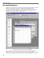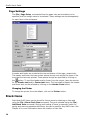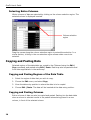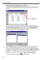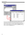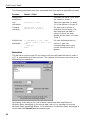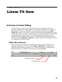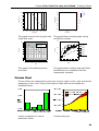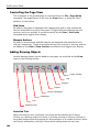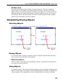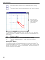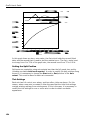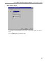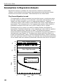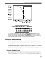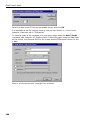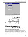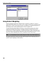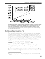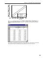
1
Erithacus Software GraFit User’s Guide Version 4.0 © Erithacus Software Limited, 1989–1998 Program and Manual Designed and Written by Robin J. Leatherbarrow GraFit User’s Guide Copyright Copyright © Erithacus Software Limited, 1989–1998. All rights reserved. Portions of the software described in this document copyright © Microsoft Corporation 1985–1998. All rights reserved. Information in this document is subject to change without notice and does not represent a commitment on the part of Erithacus Software Limited. The software is furnished under a license agreement, and the software may be used or copied only in accordance with the terms of the agreement. The purchaser may make one copy of the software for backup purposes. No part of this publication may be reproduced, transmitted, stored in a retrieval system, or translated into any language in any form or by any means, including photocopying and recording for any purpose other than the purchaser‘s personal use without the written permission of Erithacus Software Limited. Erithacus Software Limited PO Box 35, Staines Middlesex, TW18 2TG, UK VERSION 4 Last revision October 1998 Trademarks GraFit is a trademark of Erithacus Software Limited. Microsoft, Windows, NT are trademarks or registered trademarks of Microsoft Corporation. Other brands and products are trademarks or registered trademarks of their respective holders and should be noted as such. Citing GraFit in Publications When citing GraFit, simply treat this software publication as you would a book. For example: Leatherbarrow, R.J. (1998) GraFit Version 4.0, Erithacus Software Ltd., Staines, U.K. ii Version 4 is dedicated to Catherine (right) and Emma; new features that have been added since version 3 was released… iii GraFit User’s Guide Acknowledgements Version 4 Well, it took rather longer than I anticipated, but version 4 has finally appeared. The changes from version 3 are far more substantial than a single version number increment may lead one to believe, and represent a radical overhaul to the program. There are many people to thank for their encouragement and assistance, and I would like to mention some of those who have contributed most. Paul Edwards has suffered the various buggy beta versions with great tolerance, and many useful additions have been due to him. My thanks also go to Walter Ward for his help and sound advice. Steve Clarke has made a large number of valuable suggestions, and I am very grateful to Ron Duggleby for his comments and encouragement. Plaudits also to Alessandro Aliverti, Ian Auld, Bogdan Bogdanov, Bjarke Ebert, John Gebler, Florence Guye, Douglas Kell, and Karsten Olsen, for many recommendations and suggestions. As usual, Marcella has been longsuffering in her support, without which this version would still be in development. April 1998, London ROBIN J. LEATHERBARROW Version 3 Many of the improvements in this version are due to the excellent suggestions that have come from various GraFit users. My thanks to all who contributed, particularly to Pietro Belfiore, John Gebler, Douglas Kell, Steve Matthews and David Tew for many valuable recommendations, and to Martin Reddington, Walter Ward, Tim Wells and Marcella, for their continued advice. Version 2 My thanks to the many people who have given advice for improving the program. In particular, I am grateful to Bjarke Ebert, Bernard Mangold, Sanjoy Ray, Martin Reddington, Walter Ward and Tim Wells for many constructive suggestions. Once again, this program and manual would not have been possible without the help and encouragement of Marcella. Version 1 In the preparation of this program I have benefited from encouragement and advice from many sources. My thanks to all my friends and colleagues who have given help and advice, including all the members, past and present, of the Biological Chemistry section, Dept. of Chemistry, Imperial College of Science, Technology and Medicine, London U.K., especially Alan Russell, Tim Wells, Alan Fersht and Sanjoy Ray. I am particularly indebted to my wife, Marcella, who proofread the manual and put up with the ups and downs associated with program development. iv Contents Introduction ..............................................................................................1 Welcome ............................................................................................. 1 Key Features of GraFit .......................................................................... 1 About this Guide .................................................................................. 2 Notational Conventions ................................................................. 2 Contacting Erithacus Software................................................................ 2 Address ...................................................................................... 2 Technical Support ........................................................................ 3 Internet ...................................................................................... 3 Installation ................................................................................................5 System Requirements ........................................................................... 5 The GraFit Package ............................................................................... 5 Installing GraFit ................................................................................... 6 CD-ROM Installation ..................................................................... 6 Installation from Floppy Disks ........................................................ 7 Uninstalling GraFit ................................................................................ 7 GraFit Basics ..............................................................................................9 Running GraFit ..................................................................................... 9 The GraFit Workspace ......................................................................... 10 GraFit Items ...................................................................................... 11 Managing Items ......................................................................... 11 Item Representation ................................................................... 11 Editing the Item Name ................................................................ 12 Changing the Item Icon .............................................................. 12 Item-specific Commands ............................................................. 13 Printing the Item Contents................................................................... 13 Page Settings ............................................................................ 14 Stock Items ....................................................................................... 14 GraFit Templates ................................................................................ 15 Accessing Help ................................................................................... 15 Working with Files ...................................................................................17 GraFit Workspace Files ........................................................................ 17 Opening an Existing File .............................................................. 17 Saving a File .............................................................................. 18 Loading and Saving Individual Items ............................................ 18 Creating a New File .................................................................... 18 Importing Data Files ................................................................... 18 GraFit Template Files .......................................................................... 19 v GraFit User’s Guide Template Directories .................................................................. 19 Data Tables .............................................................................................. 23 The Data Table Item ........................................................................... 23 Data Types ........................................................................................ 24 Forcing Text Entry ...................................................................... 26 Moving the Data Entry Position ............................................................ 26 Selecting Regions of the Data Table ...................................................... 27 Selecting Part of the Data Table ................................................... 27 Selecting Entire Columns ............................................................ 28 Copying and Pasting Data ................................................................... 28 Copying and Pasting Regions of the Data Table .............................. 28 Copying and Pasting Columns ...................................................... 28 Removing Data .................................................................................. 30 Clearing a Region of Data............................................................ 30 Deleting a Region of Data ........................................................... 31 Inserting Values into the Table............................................................. 31 Sorting Data ...................................................................................... 32 Data Table Appearance ....................................................................... 32 Colors and Fonts ........................................................................ 32 Number Format ......................................................................... 32 Magnification ............................................................................. 34 Importing and Exporting Data .............................................................. 34 Importing Data .......................................................................... 34 Importing Data as a New Data Table ............................................ 34 Exporting Data .......................................................................... 35 Column Types .................................................................................... 35 (General) Column Type ............................................................... 37 Data Types................................................................................ 37 Column Combinations ................................................................. 39 Statistics................................................................................... 39 Data Fitting ............................................................................... 43 Calculated Values ....................................................................... 46 Data Processing ......................................................................... 50 Locking a Data Column ....................................................................... 54 Non-linear Fit Item .................................................................................. 55 Overview of Non-linear Fitting.............................................................. 55 Status Bar Indicators .................................................................. 55 Settings Pane .................................................................................... 56 Equation ................................................................................... 56 Weighting ................................................................................. 56 Data Table ................................................................................ 56 Data Layout .............................................................................. 57 X Data Column .......................................................................... 58 Y Data Column .......................................................................... 59 Error Column ............................................................................. 59 vi Contents Constants Pane .................................................................................. 59 Estimatrix Pane .................................................................................. 59 Interactive Estimator .................................................................. 60 Fitting Criteria Pane ............................................................................ 61 Fitting Criteria ........................................................................... 62 Results Pane ...................................................................................... 63 Number Format Pane .......................................................................... 64 Fonts and Indents Panes ..................................................................... 65 Formatting Item Windows .......................................................................67 Formatting Options ............................................................................. 67 Fonts Pane ........................................................................................ 67 Indents Pane ..................................................................................... 68 Linear Fit Item .........................................................................................69 Overview of Linear Fitting .................................................................... 69 Status Bar Indicators .................................................................. 69 Settings Pane..................................................................................... 70 Equation ................................................................................... 70 Weighting.................................................................................. 70 Data Table ................................................................................ 70 Data Layout............................................................................... 71 X Data Column .......................................................................... 71 Y Data Column ........................................................................... 71 Error Column ............................................................................. 71 Results Pane ...................................................................................... 72 Fonts and Indents Panes ..................................................................... 73 Equation Item ..........................................................................................75 Overview of Equation Definitions .......................................................... 75 Status Bar Indicators .................................................................. 75 General Pane ..................................................................................... 76 Changing Font Styles .................................................................. 76 Inserting OLE Objects ................................................................. 76 Editing OLE Objects .................................................................... 77 X Variables Pane ................................................................................ 77 Naming Rules ............................................................................ 78 Number of X Variables ................................................................ 78 Parameters Pane ................................................................................ 79 Constants Pane .................................................................................. 79 Definition Pane ................................................................................... 80 Equation Definition Syntax .......................................................... 81 Multi-line Equation Definitions ...................................................... 84 Use of Temporary Variables ......................................................... 84 Conditional Statements ............................................................... 84 Comments................................................................................. 85 Looping Statements.................................................................... 85 vii GraFit User’s Guide Goto Statement ......................................................................... 85 Estimates Pane .................................................................................. 86 The Need for Starting Estimates .................................................. 86 Method Used to Obtain Initial Estimates ........................................ 86 The Estimates Pane .................................................................... 87 Compiling the Equation ....................................................................... 88 Transformation Item ............................................................................... 89 Overview of Transformation Definitions ................................................. 89 Status Bar Indicators .................................................................. 90 General Pane ..................................................................................... 90 Data Points Pane ................................................................................ 91 Data Transformation Definitions ................................................... 91 Axis Name Settings .................................................................... 92 Curve Pane ........................................................................................ 92 Transformed Curve Definition ...................................................... 93 Fonts and Indents Panes ..................................................................... 94 Compiling the Transformation .............................................................. 94 Notepad Item .......................................................................................... 95 Uses of Notepad ................................................................................. 95 The Notepad Item Window .................................................................. 95 Alternatives to the use of Notepad Items .............................................. 95 Creating Graphs ....................................................................................... 97 How to Create a New Graph ................................................................ 97 Available Graph Types ........................................................................ 97 X/Y Scatter Graph ...................................................................... 98 Column Chart ............................................................................ 99 Bar Chart ................................................................................ 100 Histogram ............................................................................... 100 Graph Item ............................................................................................ 103 Overview of Graph Items .................................................................. 103 Controlling the Page View ......................................................... 104 Adding Drawing Objects ............................................................ 104 Manipulating Drawing Objects ............................................................ 105 Selecting Objects ..................................................................... 105 Moving Objects ........................................................................ 105 Sizing Objects ......................................................................... 105 Common Actions ...................................................................... 107 Grouping Objects ..................................................................... 108 Aligning Objects ....................................................................... 108 Setting the Z-Order .................................................................. 108 Setting the Object Color............................................................ 109 Setting Text Properties ............................................................. 109 General Object Properties.................................................................. 110 viii Contents Fill Properties........................................................................... 111 Line Properties ......................................................................... 111 Rotation Properties ................................................................... 112 Location Properties ................................................................... 112 Arrows Properties ..................................................................... 113 Font Properties ........................................................................ 113 Paragraph Properties ................................................................ 114 X/Y Scatter Graphs ................................................................................115 The XY Graph Wizard ........................................................................ 115 Select Data Source Page ........................................................... 115 Set Initial Scaling ..................................................................... 117 Select Tick Styles ..................................................................... 118 Select Data Point Style ............................................................. 118 Enter Curve Parameters ............................................................ 119 Enter Curve Constants .............................................................. 120 Select Fitting Curve Style .......................................................... 120 Select Join Style....................................................................... 121 Modifying Graphs ............................................................................. 122 Selectable Regions of a Graph ................................................... 123 Main Graph Region ........................................................................... 123 General Page ........................................................................... 124 Fill Page .................................................................................. 125 Line Page ................................................................................ 125 X Ticks Page ............................................................................ 125 X Scale Page............................................................................ 127 Y Ticks Page ............................................................................ 129 Y Scale Page ............................................................................ 129 Location Page .......................................................................... 129 Axis Scale Regions ............................................................................ 130 Scale Page .............................................................................. 130 Axis Text Regions ............................................................................. 132 Legend Box Region ........................................................................... 132 Legend Page ............................................................................ 132 Fill Page .................................................................................. 133 Line Page ................................................................................ 133 Location Page .......................................................................... 133 Data/Curve Properties ....................................................................... 134 Data Points Page ...................................................................... 134 Join Points Page ....................................................................... 135 Fitted Curve Page ..................................................................... 136 Data Source Page ..................................................................... 137 Data Source Page ..................................................................... 138 Error Bars Page ........................................................................ 139 Axis Association Page ............................................................... 142 Equation Page .......................................................................... 143 ix GraFit User’s Guide Parameters Page ...................................................................... Constants Page ........................................................................ Legend Text Regions ........................................................................ Adding Extra Data to the Graph ......................................................... Set Axis Associations Page ........................................................ 143 144 144 144 145 Using Multiple Graph Axes ..................................................................... 147 When to Use Multiple Axis Scaling ...................................................... 147 Overlaying Data that have Different Scales ................................. 147 Split Axes ............................................................................... 148 Creating and Managing Multiple Axes .................................................. 148 Running the Axis Manager ......................................................... 148 Adding a New Axis ................................................................... 149 Splitting an Existing Axis ........................................................... 150 Removing an Axis .................................................................... 151 Working with Multiple Axes ................................................................ 152 Axis Text and Axis Scale Text .................................................... 152 Data Association ...................................................................... 152 Axis Scaling and Sizing ............................................................. 153 Column and Bar Charts .......................................................................... 157 The Chart Wizard ............................................................................. 157 Select Data Source Page ........................................................... 157 Set Initial Scaling ..................................................................... 159 Select Tick Styles ..................................................................... 160 Select Bar Style ....................................................................... 161 Select Data Point Style ............................................................. 162 Select Join Style ...................................................................... 163 Histograms ............................................................................................ 165 The Histogram Wizard....................................................................... 165 Select Data Source Page ........................................................... 165 Set Initial Scaling ..................................................................... 166 Select Tick Styles ..................................................................... 167 Select Bar Style ....................................................................... 167 Embedding and Linking ......................................................................... 169 What is Embedding and Linking? ........................................................ 169 Original Cut and Paste Model ..................................................... 169 Embedded Objects ................................................................... 170 Linked Objects ......................................................................... 170 Using Embedding and Linking ............................................................ 170 Comparison of Data Transfer Types ............................................ 171 Embedding and Linking without using the Clipboard ..................... 172 Embedding and Linking with GraFit ..................................................... 172 GraFit as an OLE container ........................................................ 173 GraFit as an OLE source ............................................................ 173 x Contents Data Fitting Basics .................................................................................175 When Is Data Fitting Appropriate? ...................................................... 175 Types of Data .......................................................................... 175 Regression Analysis .......................................................................... 177 Practical Considerations ............................................................ 177 Types of Regression Analysis ..................................................... 178 Linear Regression ............................................................................. 178 Polynomial Regression .............................................................. 178 Non-linear Regression ....................................................................... 178 Additional Considerations for Non-linear Regression ..................... 178 Weighting Scheme ............................................................................ 179 Linear Regression of Transformed Data ............................................... 179 Information Obtained from Data Fitting ............................................... 180 Multiple Regression ........................................................................... 181 Uses for Multiple Regression ...................................................... 181 Advantages of Multiple Regression.............................................. 182 Disadvantages of Multiple Regression ......................................... 182 Defining Equations ................................................................... 182 Fitting Data by Multiple Non-linear Regression ............................. 182 Data Fitting ............................................................................. 184 Plotting Results from Multiple Regression .................................... 184 Theory ...................................................................................................185 Regression Analysis .......................................................................... 185 Assumptions in Regression Analysis .................................................... 186 Linear Regression ............................................................................. 187 Weighting................................................................................ 188 Weighting Types............................................................................... 189 Non-linear Regression ....................................................................... 190 Standard Errors of the Calculated Parameters .............................. 190 Robust Weighting ............................................................................. 190 Determining the Most Appropriate Weighting ....................................... 192 Plot of Residual Errors............................................................... 193 Testing Goodness of Fit — F Test ........................................................ 193 Mean and Standard Deviation ............................................................ 193 Worked Data Fitting Examples ...............................................................195 Using One of the Equations Provided ................................................... 195 Fitting the Data ........................................................................ 196 Checking the Weighting ..................................................................... 199 Drawing Residual Plots .............................................................. 199 Using Robust Weighting .................................................................... 202 Defining a New Equation (1) .............................................................. 203 Defining the Oxygen Binding Equation ........................................ 204 Defining a New Equation (2) .............................................................. 206 Defining the Equation ............................................................... 207 Fitting the Equation .................................................................. 207 Multiple Regression ........................................................................... 208 xi GraFit User’s Guide Displaying Multidimensional Data ............................................... 209 Reading Values from a Calibration Curve ............................................. 211 Choosing an Equation to Fit the Data .......................................... 211 Reading Values from the Fitted Curve ......................................... 213 Fitting Several Data Sets with Some Parameters Common and Some Specific ...................................................................................................... 213 Method Used to Share Variables Between Data Sets ..................... 214 Example — Paired Denaturation Curves ...................................... 216 Equations Provided ................................................................................ 219 2 Substrates .................................................................................... 220 Ping pong ............................................................................... 220 Ping pong Lineweaver Burk ................................................... 220 Ternary .................................................................................. 220 Ternary Lineweaver Burk .......................................................... 220 Enzyme Inhibition ............................................................................ 221 Competitive Inhibition .............................................................. 221 Competitive Eadie Hofstee ........................................................ 221 Competitive Lineweaver Burk .................................................... 221 Mixed Inhibition ....................................................................... 221 No inhibition ............................................................................ 221 Non-competitive Inhibition ........................................................ 222 Non-competitive Eadie Hofstee .................................................. 222 Non-competitive Lineweaver Burk .............................................. 222 Enzyme Kinetics ............................................................................... 222 Allosteric kinetics (Hill) ............................................................. 222 Allosteric kinetics (Hill), Linear plot ............................................ 222 Enzyme Kinetics ...................................................................... 223 Enzyme Kinetics, Eadie Hofstee ................................................. 223 Enzyme Kinetics, Lineweaver Burk ............................................. 223 Enzyme Kinetics, show Km ........................................................ 223 Enzyme Kinetics, show Vmax .................................................... 223 Enzyme Kinetics, show Vmax over Km ........................................ 223 Kinetics, contaminating S .......................................................... 224 Exponential ..................................................................................... 224 Double Exponential .................................................................. 224 Double Exponential - phase 1 .................................................... 224 Double Exponential - phase 2 .................................................... 224 Double Exponential with offset ................................................... 224 Single Exponential ................................................................... 225 Single Exponential with offset .................................................... 225 Triple Exponential .................................................................... 225 Triple Exponential with offset..................................................... 225 IC 50 .............................................................................................. 225 IC50 0-100% .......................................................................... 225 IC50 0-100% - show IC50 ........................................................ 226 xii Contents IC50 background corrected ....................................................... 226 IC50 background corrected - show IC50 ..................................... 226 IC50 background corrected - show limit ...................................... 226 IC50 full 4 param ..................................................................... 226 IC50 full 4 param - show background ......................................... 227 IC50 full 4 param - show IC50 ................................................... 227 IC50 full 4 param - show limit.................................................... 227 Ligand Binding ................................................................................. 227 1 Site ..................................................................................... 227 1 Site – Scatchard Plot.............................................................. 228 1 Site – Show Capacity ............................................................. 228 1 Site – Show Kd (1 site) .......................................................... 228 1 Site (with background) ........................................................... 228 1 Site (with background) - Scatchard.......................................... 228 1 Site (with background) - Show background .............................. 228 1 Site (with background) - Show Capacity ................................... 228 1 Site (with background) - Show Kd ........................................... 229 2 Site ..................................................................................... 229 2 Site - Show Capacity (total) .................................................... 229 2 Site - Show Capacity 1 ........................................................... 229 2 Site - Show Curve 1 ............................................................... 229 2 Site - Show Curve 2 ............................................................... 229 2 Site (with background) ........................................................... 229 2 Site (with background) - Show background .............................. 229 2 Site (with background) - Show Capacity 1 ................................ 230 2 Site (with background) - Show Capacity (total) ......................... 230 2 Site (with background) - Show Curve 1 .................................... 230 2 Site (with background) - Show Curve 2 .................................... 230 Adair (2 sites) .......................................................................... 230 Adair (3 sites) .......................................................................... 230 Adair (4 sites) .......................................................................... 230 Bound vs Total ......................................................................... 231 Bound vs Total - tight binding limit ............................................. 231 Cooperative ............................................................................. 231 Cooperative (with background) .................................................. 231 pH .................................................................................................. 232 pKa, (min = 0) ........................................................................ 232 pKa, (min = 0), Linearized Plot .................................................. 232 pKa, (min = 0), Show Limit ....................................................... 232 pKa, (min = 0), Show pKa ......................................................... 232 pKa, (min = 0), High to Low ...................................................... 232 pKa, (min = 0), High to Low, Show Limit .................................... 232 pKa, (min = 0), High to Low, Show pKa ...................................... 233 pKa, Double ............................................................................ 233 pKa, Double, Show Curve 1 ....................................................... 233 pKa, Double, Show Curve 2 ....................................................... 233 xiii GraFit User’s Guide pKa, Double, Show Limit 1 ........................................................ pKa, Double, Show Limit 2 ........................................................ pKa, Double, Show Limit 3 ........................................................ pKa, Double Bell ...................................................................... pKa, Double Bell, Curve 1 ......................................................... pKa, Double Bell, Curve 2 ......................................................... pKa, Double Bell, Limit ............................................................. pKa, Single ............................................................................. pKa, Single, Linearized plot ....................................................... pKa, Single, Show Limit 1 ......................................................... pKa, Single, Show Limit 2 ......................................................... pKa, Single, Show pKa.............................................................. Rate ............................................................................................... 1st order................................................................................. 1st order, decay curve .............................................................. 1st order, show limit ................................................................ 1st order, show initial ............................................................... 1st order (offset) ..................................................................... 1st order (offset), decay curve .................................................. 1st order (offset), show limit ..................................................... 1st order (offset), show offset ................................................... 1st order rate versus [S] .......................................................... 1st order rate versus [S] (offset) ............................................... 233 233 233 233 234 234 234 234 234 234 234 234 235 235 235 235 235 235 235 236 236 236 236 Standard Templates ............................................................................... 237 About the Standard Templates ........................................................... 237 Accessing Templates ................................................................ 237 Template Layout ...................................................................... 238 Using Your Own Templates ........................................................ 238 Description of the Standard Templates................................................ 239 Enzyme Kinetics ...................................................................... 239 IC 50 ...................................................................................... 240 Ligand Binding ......................................................................... 241 Linear Regression .................................................................... 242 Single Exponential ................................................................... 243 GraFit Symbols Font .............................................................................. 245 GraFit Symbols Font ......................................................................... 245 Index ..................................................................................................... 247 xiv C H A P T E R 1 Introduction Welcome GraFit version 4 for Microsoft® Windows™ combines presentation-quality scientific graphs with comprehensive data fitting. The result is a powerful package that is easy to use, produces stunning output, and can also fulfil the needs for quantitative data analysis. Data can be fitted using various types of theoretical models, and your own equations can easily be added to those supplied with the program. Comprehensive graph plotting facilities allow you to display your data on-screen and edit the graphs interactively. Key Features of GraFit GraFit provides the experimental scientist with a tool for visualization and analysis of their data. For the occasional user, GraFit can be configured to perform routine analyses with minimal intervention—in many cases it is possible just to enter the data and allow GraFit to calculate the results and plot the graphs in the background. Advanced users can utilize the full power of GraFit for analyzing complex equations, and may create custom fitting templates for routine data processing. 1 GraFit User’s Guide About this Guide This manual describes how you can use GraFit to examine your data, and to plot graphs. We recommend that you read the manual fully, and try out some of the examples described. Notational Conventions The following notational conventions are used throughout this manual: Convention Meaning SMALL CAPITALS Small capitals indicate keys to be pressed. For instance, A indicates ―press the ‗A‘ key‖. If more than one key needs to be pressed this is written as (for instance) SHIFT END which would mean ―hold down the ‗Shift‘ key and then press the ‗End‘ key‖. Monospace Monospace type indicates text that should be entered on the computer keyboard. For example, to obtain a directory of drive A: when in DOS you would enter DIR A: RETURN Bold Bold text is used for menu item commands, e.g. the Edit menu. Where cascading menus are present, a vertical bar (|) is used to separate the sub-menus. For example, the Windows Control Panel application is started from the desktop Start | Settings | Control Panel command. Important information that should be noted is written in italics, and separated from other text by horizontal rules, as here. Contacting Erithacus Software Address Erithacus Software Limited PO Box 35 Staines Middlesex TW18 2TG UK 2 Chapter Error! AutoText entry not defined.: Introduction Technical Support At Erithacus we are working hard to provide you with intuitive technical products. However, if you find yourself with a technical question that you cannot resolve, please contact our technical support department. Registered users can obtain technical support from one of the following sources: Fax: [+44] (0)1784 442005 Email: [email protected] Internet: http://www.erithacus.com Note: Always quote your serial number and the product version, which are shown on the About screen (Help | About GraFit command). Internet Our web site can be found at http://www.erithacus.com and here you will find latest information about our software products. In addition, we post technical notes, tips and answers to common problems. Tip: Be sure to check out http://www.erithacus.com to download the latest fixes and updates. 3 GraFit User’s Guide 4 C H A P T E R 2 Installation System Requirements Software GraFit version 4 is a fully 32-bit program that requires Windows 95 or later, or Windows NT 4.0 or later. It is not compatible with Windows 3.1 or earlier. The Help system requires installation of Microsoft Internet Explorer version 3.02 or later. Microsoft Internet Explorer version 4.01 is supplied with GraFit, and it is recommended that you install this before installing GraFit. Hardware The minimum hardware required is a PC with a 66 MHz 486 processor with 8 Mbytes RAM, and the recommended configuration is a 100 MHz Pentium with 16 Mbytes RAM or better. You need at least 10 Mbytes free space on your hard disk drive, and a mouse (or compatible pointing device). A CD-ROM drive is highly recommended, and although installation from 3½" disks is possible, 3½" media are not supplied as standard (see Installing GraFit for details on obtaining GraFit on 3½" disks). The CD-ROM includes optional tutorial files in the form of screencapture movies; these files make use of sound, and so to view these you need a PC with a Windows-compatible sound system. The GraFit Package The GraFit package comprises the following: GraFit program CD-ROM. The GraFit User‘s Guide (this manual). Depending upon the GraFit package that was purchased, this guide may only be available in electronic form on the CDROM. When GraFit is first run you will be able to register the product. This will ensure that you are informed of the latest updates to the program. 5 GraFit User’s Guide Installing GraFit CD-ROM Installation Insert the GraFit CD-ROM into your CD drive. The Welcome screen will load automatically. Note: Some systems are configured so that automatic running of CD-ROM software is disabled. If your system is set up in this way, the Welcome screen can be displayed by selecting the Run command from the Windows Start menu, and entering the command D:\CDRUN where D: is the drive letter of your CD-ROM. Microsoft Internet Explorer GraFit uses a new HTML help system that will become a standard feature in the next generation of Windows. To use this help system, it is necessary to have Microsoft Internet Explorer (version 3.02 or later) installed on your computer. If you do not already have this software installed, select the Install Internet Explorer 4 option and follow the instructions. Note: The installation of Internet Explorer will update some of the system files on your computer. If you are running Windows NT this will require Administrator privileges. Please consult your computer administrator if your account does not allow you to do this. GraFit Select the Install GraFit option to install GraFit onto your computer. The installation program will copy the files to your hard disk, and place an entry for the GraFit program on the Start button, under the Programs entry. Adobe Acrobat Reader The GraFit CD-ROM includes this user manual saved in Adobe Portable Document Format (PDF). If you wish to read this file, it is necessary to have the Adobe Acrobat Reader (version 3 or later) installed. If you do not already have this software installed, you can choose to do so by selecting Install Acrobat Reader. 6 Chapter Error! AutoText entry not defined.: Installation Installation from Floppy Disks GraFit is shipped as standard on CD-ROM, and no floppy disk media are provided. If you do not have a CD drive on your system, it is possible to install GraFit by one of the following routes: The program on 3½" disks is available from Erithacus Software for a nominal charge that covers media costs, plus postage and handling. Please contact Erithacus Software for pricing and availability (contact details are given in Chapter 1). It is possible to create a set of 3½" installation disks if you have access to another computer with a CD drive. You will need a number of blank, formatted 3½" disks. To create this disk set, double-click on the ―Make Floppy Disk Set‖ file located in the root directory of the GraFit CD. Note: GraFit on floppy disk only includes the main GraFit program file. The CDROM version also includes electronic documentation and tutorials that are too large for 3½" media. Uninstalling GraFit GraFit can be removed from your system by the following procedure. 1. From the Windows Start menu, launch the Control Panel application from the Settings sub-menu. 2. Double-click the Add/Remove Programs icon. 3. Choose GraFit 4 to uninstall, and click the Add/Remove button. 4. Follow the instructions 7 GraFit User’s Guide 8 C H A P T E R 3 GraFit Basics Running GraFit The GraFit installation program will add a GraFit entry to the Programs list on your Windows Start menu. When you run the GraFit program, the main GraFit window will open. Workspace toolbar, item buttons Project window When initially opened, the GraFit workspace is empty. 9 GraFit User’s Guide The GraFit Workspace A GraFit file can comprise one or more data tables, graphs, data analyses, equation definitions, transformation definitions, notepads and embedded objects. Collectively, these items make up the GraFit workspace, which can be stored to disk as a single file. After adding a number of items to the workspace, the appearance of the GraFit window is shown below. A GraFit workspace with a number of items added In this example, one each of the following items has been added: a data table; a graph window; a non-linear fitting item; a linear fitting item; an equation definition; a notepad; a transformation definition and an embedded Microsoft Word 10 Chapter Error! AutoText entry not defined.: GraFit Basics document. All the added items are stored inside the same GraFit workspace, and can be saved and loaded from disk using the File menu commands. If you run a second copy of GraFit, you can copy items between workspaces by drag and drop or by using the commands on the Edit menu to copy and paste items via the Windows Clipboard. Each item in the workspace is represented by an icon in the project window. GraFit Items GraFit items are initially created in a new window that residues within the main GraFit window, and are identified by the presence of an icon in the project window. Closing an item window does not delete the item — it simply makes the window invisible. This allows you to keep open only those items that you are currently working on. Managing Items Adding New Items To add a new item to the workspace: Use the Add menu, or click on the item buttons in the workspace toolbar. Switching Between Items To switch between items: Click on the window to activate, or click on the icon that represents this item in the project window. Removing Items To delete an item from the workspace: Select the icon that represents the item in the project window, and choose the Edit | Clear command. Item Representation When an item window is closed, the contents of the item still remain present in the GraFit workspace file. The item window can be reopened by double-clicking on the icon. The icon that represents the item is shaded so that it indicates the current state of the item, as shown below. 11 GraFit User’s Guide GraFit item, open. The icon is drawn normally. GraFit item, closed. The icon is drawn as a ghosted image, which is lighter than normal. Embedded object, open for editing. The object icon is shown overdrawn with hatched lines. Embedded object, closed. The icon is drawn ghosted. Linked object, closed. A shortcut overlay ( ) is added to the icon. Switch between item windows to edit their contents. Information about using each of the GraFit item types is found in Chapters 5-13. Editing the Item Name Items are referred to by the name shown in the project window, so it is useful to change this from the default to something more meaningful. To edit the item name, select the icon in the project window, and choose the Edit | Rename command. Type in the new name. Item names can contain any characters, but must be different from any other item name in the workspace. Changing the Item Icon The icon that represents an item may also be changed. This can be useful to allow similar items to be visually distinguished. To change the icon, select it and choose the Window | Icon command. For each item type there are a number of alternative images that can be used. In addition, it is possible to use an icon image that resides in any executable or DLL file on your computer. 12 Chapter Error! AutoText entry not defined.: GraFit Basics Item-specific Commands Although some commands apply to all GraFit items, many are item-specific. For example, the Fit Data command applies to the Linear fit and Non-linear fit items, but not to the Data table or Graph items. Commands that are not available are shown grayed. In addition, each item window has one or more specific menus that are only present when this window is selected. For example, only graph items have Graph and Object menus. Printing the Item Contents The contents of any item window can be printed using the File | Print command, and the printing previewed using the File | Print Preview command. Print preview 13 GraFit User’s Guide Page Settings The File | Page Setup command allows the paper size and orientation to be specified, and the margin sizes to be entered. These settings are stored separately for each item in the workspace. A header and footer are printed at the top and bottom of the page, respectively. The header and footer text can contain special strings such as the file name or the time that the item was printed. These special strings are specified by clicking on the button. To omit the header and/or footer from the output, leave the entries for the Header text and/or Footer text blank. The font used to display the header and footer text can be selected by clicking on the Header Fonts button. Changing the Printer To change the printer from the default, click on the Printer button. Stock Items Individual GraFit items can be stored for future reuse by selecting an item and using the File | Store Stock Item command. They are reloaded using the File | Add Stock Item command. Storing and loading of items is especially useful for saving and restoring equation definitions, but can be used for any GraFit item. See Chapter 4 for more information about the location of item files. 14 Chapter Error! AutoText entry not defined.: GraFit Basics GraFit Templates Workspace files can be created by adding a number of items as described above. Alternatively, it is possible to load a pre-built workspace from a template, using the File | New command. See Chapter 4 for more information about using templates. Accessing Help GraFit includes a complete on-line help system to guide you through learning the product. To view the help topics: From the Help menu, select the Contents command. To obtain specific help on the function of a menu item, toolbar command or window item: Click on the Context Help toolbar button further information is required. and then on the item for which To obtain specific help within a dialog box: Click on the Context Help button in the top right of the dialog box and then on one of the items in the dialog box. Context sensitive help gives specific information on each item within the dialog box 15 GraFit User’s Guide 16 C H A P T E R 4 Working with Files GraFit Workspace Files The GraFit workspace consists of all the items displayed in the main GraFit window (data tables, graphs etc.). The contents of the workspace are stored together in a GraFit workspace file, which has the .GFF extension. In addition to the contents of the workspace, the current window sizes and positions are also stored in the workspace file. Opening an Existing File Choose the File | Open command to open an existing GraFit workspace file. This will bring up the Open dialog box, as shown below. The buttons marked User Data and User Template allow you to change directory rapidly to the default data and user template directories respectively. (The locations of these special directories are chosen from the View | Options menu.) By default, GraFit workspace files are listed, but you can elect to display (and open) GraFit template files by changing the Files of type selection. 17 GraFit User’s Guide Saving a File GraFit workspace files are saved using the File | Save or File | Save As commands. The contents of the workspace are saved, along with the current window positions and order. When the file is reloaded, these positions and order are restored. Loading and Saving Individual Items Saving Items The GraFit workspace comprises a number of individual items, such as data tables, graphs and analyses. These individual items are saved in one of the following ways: Select the item in the Project window, then issue the File | Store Stock Item command. From the open item window, select the File | Store Stock Item command. By default, items should be saved in the item store directory, or a subdirectory off this. (The location of the item store directory is specified using the View | Options command.) Loading Items Stored items can be loaded using the File | Add Stock Item command. Creating a New File To reset the GraFit workspace: Click on the File New toolbar item Note . This command is different to the File | New menu command, which loads a new file based on a template. Importing Data Files Data can be imported into GraFit to create a new data table item that holds the imported data. To create this item, select the File | Import Data command from the main GraFit window. Any file for which a filter is available can be imported into GraFit (see the following section on Import/Export Filters). It is also possible to paste data from a file directly into an open data table. To do this, use the Edit | Paste From command of the data table item. 18 Chapter Error! AutoText entry not defined.: Working with Files Import/Export Filters In order to perform conversions between GraFit and other data types, GraFit uses installable import/export filter files. Several standard filter types are supplied by default with GraFit, and other filters may be available from certain instrument manufacturers or from Erithacus Software. These filter files are installed into GraFit from the View | Options dialog box, Data Filters tab. Please contact Erithacus Software if you have special requirements for a specific filter file. GraFit Template Files Template files are pre-made workspace files that are used to speed up use of common procedures. Template files differ from workspace files in the following ways. They are represented by a different icon. Double-clicking on a template file opens a copy of the file rather than the file itself. Templates stored in the user or group template directories can be rapidly accessed using the File | New command. Creating a Template File To store a workspace as a template file, select the File | Save As command, and save as type ―GraFit Template Files.‖ If you wish to access this template using the File | New command, ensure that the file is saved into your user or group template directory (see the following section on Template Directories). To help with this, the Save As dialog box contains a command button that will jump immediately to your user template directory. Creating a File Based on a Template The File | New command creates an untitled file based on a selected template. This command in described in the following section. Chapter 23 describes the standard templates that come pre-defined with GraFit. Template Directories There are two directories that have special significance when storing template files. These are the user and group template directories, the location of which is specified from the View | Options command, Directories tab: 19 GraFit User’s Guide Click on the button to change a directory setting. By having two separate locations for templates it is possible to keep user-specific files separate from general templates that are used by a group of users. It can be useful, as illustrated above, to maintain a group directory on a network server. Files in a template directory appear on the General tab of the File | New dialog box. Any subdirectories have special significance, and result in additional tabs on this dialog; clicking on the tab accesses the files in these subdirectories. (Note that empty subdirectories do not appear). 20 Chapter Error! AutoText entry not defined.: Working with Files The files displayed on this dialog box are the sum of those present in the user and the group template directories. (The specific location of any individual file can be found by right-clicking on the icon, and choosing the Properties command. In the event that a file with the same name is found in both the user and group directories, the user file has precedence.) To create a new workspace file based on one of these templates, select the one to use and click OK. 21 GraFit User’s Guide 22 C H A P T E R 5 Data Tables The Data Table Item To add a new, empty data table to the GraFit workspace: Click the data icon on the Workspace toolbar Table command. , or select the Add | Data The parts of the data table window are shown in the following illustration. Column selection region Column resize region Type indicator row Column heading Data entry position Splitter box Row selection region Position row 1 column 1 in the above figure is marked by a dark outline; this is the current data entry position. Data entries are edited in situ by typing in the new entry. When the entry is complete, pressing RETURN, TAB or a cursor key, or clicking the mouse on a different position in the data table, will accept the data, and move 23 GraFit User’s Guide the data entry position. To edit the value at the current data entry position, select the Edit | Edit Current Cell command, or press F2. The following table describes the elements in a data table. Certain sub-regions are distinguished by the mouse cursor changing shape when it is over them. Element Description Data table The data values themselves are listed in the data table. Click the mouse on a value to move the data entry position; drag the mouse to select larger regions of the data table. Newly entered data is placed at the data entry position, which can be moved using the cursor keys or by clicking the mouse on a different part of the data table. Column selection region Click and drag the mouse on the column numbers to select entire columns of data. Column resize region Click and drag the edges of a column to resize it. Row selection region Click and drag the mouse on the row numbers to select entire rows of data within the data table. Row resize region Click and drag the edges of a row to resize it. Split table horizontally Drag the splitter box on the horizontal scroll bar to divide the data table window in two. The two halves can be independently scrolled, allowing distance regions of the table to be viewed simultaneously. Split table vertically Drag the splitter box on the vertical scroll bar to divide the data table window in two. The two halves can be independently scrolled, allowing distance regions of the table to be viewed simultaneously. Cursor Resizing Rows and Columns The row height and column width can be set using the Table | Row Height and Table | Column Width commands, respectively, or by using the mouse to drag the edges of the rows or columns within the row or column selection region. Columns can be sized to fit their contents using the Table | Size Column to Fit command. Data Types The number of data points that can be entered is limited only by available memory. The data are grouped into columns, and the contents of one or more columns can be used for data fitting or graph plotting. 24 Chapter Error! AutoText entry not defined.: Data Tables Within a column, each individual cell holds a data value that may be one of three different types: Data Type Description Numbers Numbers are the most common data form that will be entered into GraFit. They are used to plot x/y scatter plots, and for data fitting by regression analysis. Very small or large numbers can be entered in exponential format, for example 1e7 is equal to 10000000, and 1e-23 represents 10-23. Note The representation of numbers, particularly the symbol used for the decimal point, differs from country to country. By default, GraFit uses the country-specific settings selected for your Windows installation (using the Control Panel application, Regional Settings). However, you can override these from the View | Options dialog box, Number Format page. Text Text entries can be used for annotation, and are also used to provide the text for the category axes of charts. Text values are treated as missing data during data fitting. Missing Data Experimental data often contain certain values that are not available (perhaps because that particular experimental sample was the one that fell on the floor!). GraFit allows you to insert ―missing‖ values by leaving the data entry blank. All the graphing and data fitting elements of the program will recognize such points, and omit them from the analysis. The representation of these different data types is illustrated in the following diagram. Text Number Missing value 25 GraFit User’s Guide Forcing Text Entry GraFit displays text items as they are entered, but formats numbers dependent upon the current column formatting (Table | Column Format command). To force numbers to be treated as a text item, enter them with a preceding ' symbol, for example: '2.34 Forcing text entry can be useful if a number is used as one of the entries in the category axis of a chart. Note Numbers forced to act as text are not available as data items, and will be treated as missing items during data fitting. Moving the Data Entry Position When you have entered your data value you will need to move to the next data entry position by pressing TAB, RETURN or DOWN after entering the value. The following keys control movement of the data entry position within the data table. To Press Move the entry point to the right TAB Move the entry point to the left SHIFT TAB Move the entry point up UP Move the entry point down DOWN Move to the first column of a row CTRL LEFT Move to the last column that contains data entries CTRL RIGHT Move to the first row of a column CTRL UP Move to the last row that contains data entries CTRL DOWN It is often convenient to press RETURN or DOWN or RIGHT or or LEFT RETURN between entering data points. Moving the data entry position using the mouse To move the data entry position using the mouse, move the mouse pointer to the position you require, and click the left mouse button. 26 Chapter Error! AutoText entry not defined.: Data Tables Selecting Regions of the Data Table Selecting Part of the Data Table To select a portion of the data table, drag the mouse over the required region. Alternatively, hold down the SHIFT key, and use the cursor keys to extend the selection. The selected region is displayed inverted, as shown below. Selected region Clicking the mouse within the row selection area results in the entire row being selected. To make a more extensive selection: Click on the start position. Use the scroll bars to move the window as necessary. Hold down the SHIFT key, then click on the end position for the selection. Discontinuous selection Hold down the CTRL key and click the required entries. 27 GraFit User’s Guide Selecting Entire Columns Whole columns of data are selected by clicking on the column selection region. The selected column is displayed inverted. Column selection region Drag the mouse along the column selection region to extend the selection. In a similar fashion, clicking in the row selection region allows whole rows to be selected. Copying and Pasting Data Selected regions of the data table are copied to the Clipboard using the Edit | Copy command, and pasted using Edit | Paste. Data may also be pasted to and from other applications in the same way. Copying and Pasting Regions of the Data Table 1. Select the region of data that you wish to copy. 2. Choose the Edit menu, and select Copy. 3. Move the data entry position to where the data is to be copied. 4. Choose Edit | Paste. The data will be inserted at the data entry position. Copying and Pasting Columns Entire columns of data can also be copied and pasted. Pasting into the data table when a column is selected results in the pasted values being placed in a new column, in front of the selected column. 28 Chapter Error! AutoText entry not defined.: Data Tables 1. Select the column(s) of data that you wish to copy. 2. Choose the Edit menu, and select Copy. 3. Select the column in front of which the data are to be inserted. 4. Choose Edit | Paste. When pasting into a fully selected column, you have the option to overwrite the selected data or to insert the new data in front of the selection (the overwrite option is only available if the number of columns available to paste is the same size as in the selected region). The data are then pasted into the table. 29 GraFit User’s Guide Removing Data Clearing a Region of Data The Edit | Clear command, or the selected data or columns. DEL key, can be used to clear the currently 1. Select the data value(s) (or columns or rows) to be cleared. 30 Chapter Error! AutoText entry not defined.: Data Tables 2. Choose Edit | Clear, or press DEL. Data in the selected region are cleared, leaving a gap in the table. Deleting a Region of Data Select the data value(s) (or columns or rows) to be cleared. Choose Table | Delete command. When deleting a range of cells, the data values are moved up so that no gap appears in the table. When deleting a column, the remaining columns to the right of the selection are moved along to fill the gap. Inserting Values into the Table Values are inserted into the data table using one of the Table | Insert commands. Command Action Table | Insert Cells Inserts blank cells in place of the current selection. Cells are moved down to accommodate the new entries. Table | Insert Column Inserts blank columns in place of the current selection. Columns are moved to the right to accommodate the new entries. Table | Insert Row Inserts blank rows in place of the current selection. Rows are moved down to accommodate the new entries. 31 GraFit User’s Guide Sorting Data The data in one or more columns can be sorted into ascending or descending order using the Table | Sort Column(s) command, after first selecting the columns that you wish to sort. The Index column selection specifies the column on which the sort order is based. In addition to this column, any of the other columns can be included in the sort by checking the box to the left of the column name. Data Table Appearance Colors and Fonts The colors used to display the items in the data table, and the font that is used to draw the table, are set using the Table | Preferences command. Number Format The manner in which numbers are formatted for display can be set on a column by column basis. The Table | Column Format command is used to control the displayed numerical precision. This command applies to all columns that fall within the current selection. 32 Chapter Error! AutoText entry not defined.: Data Tables Column Format dialog box Specification Meaning Decimal places Enter the number of decimal places to be displayed for numbers. Note To ensure that all decimal places are displayed set Trailing zeros in fraction to “Show 0’s.” Max digits Enter the maximum number of digits to use when displaying numbers. Thousands separator Check this box to include a grouping separator. The symbol used for this separator, and the number of digits in the group, are set for the View | Options command on the main GraFit window. Scientific format Check this box to display the values using scientific format (e.g. -2.435e003 instead of -2435.000). Use scientific format for small values Check this box to ensure that small values, which would otherwise be displayed as 0.0000, are shown in scientific format (e.g. 2.0987e-008). Trailing zeros in fraction Chooses the way that trailing zeros are displayed in the formatted numbers. It is possible to show the ―0‖ characters, to omit them, or to replace them with spaces. Save As Defaults Stores the current settings as the default for future GraFit sessions. Restore Defaults Restores the current GraFit formatting defaults to the selected columns. 33 GraFit User’s Guide Magnification The magnification of the data table text can be adjusted to allow more or less values to be visible. Magnification is controlled by the View | Zoom command, or by using the zoom control on the Standard toolbar. Zoom control Changing the magnification and altering the font size (Table | Preferences command) both modify the size of text displayed on-screen. However, changing font size using Table | Preferences also changes the size of printed text, while View | Zoom only affects the on-screen appearance. Importing and Exporting Data Importing Data To import data into a data table, position the data entry position where you want the data values to start and select the Edit | Paste From command. Select the file that holds the values to import, and press the Open button. The contents of the file will be inserted into the data table. Importing Data as a New Data Table It is also possible to import a file into the GraFit workspace as a new data table item. To import a data file in this way, use the File | Import Data command. 34 Chapter Error! AutoText entry not defined.: Data Tables Exporting Data To export data from a data table into a file that can be read by other programs, select the range of values to be exported and use the Edit | Copy To command. The Save as type entry determines the format in which to save the exported data. GraFit supports a number of data export formats, and the available types are listed in this box. GraFit supports export as ASCII, DIF and CSV formats as standard, though additional formats may be available. Column Types Columns can hold simple data values, or can be set to hold the results of various calculations or data manipulations. For example, a column can hold the difference between the values in two other data columns. The results of these calculations are automatically updated when the source data change, allowing powerful processing of the underlying data. 35 GraFit User’s Guide Example: setting up a difference calculation As an illustration, we will show how to set up the following data table in which the third data column holds the difference between the values in the first and second columns. Type area of column 3 The column type of the third column needs to be set by moving the data entry position to somewhere within this column and choosing the Table | Column Type | Column Combinations | A-B command. Alternatively, the Column Type submenu can be accessed by double-clicking in the type area of the column. For this column type setting, the following dialog is displayed. Choosing Value 1 as the first column and Value 2 as the second gives the result above. The values that are displayed in this column cannot be overwritten or edited, and are updated whenever the values in the source columns changes. The text color of the calculated values can be adjusted using the Table | Preferences command, but is typically shown a different color than the editable text in order to distinguish it. The dialog settings for the calculated values can be altered by repeating the command, or by choosing the Table | Column Properties command, which corresponds to the 36 toolbar command. Chapter Error! AutoText entry not defined.: Data Tables To reset the column type to the default (non-calculated) settings, choose Table | Column Type | (General). Note Even though columns that hold calculated values do not allow these values to be edited, it is always possible to modify the column name entry. (General) Column Type By default, all columns are set to be of (General) type, and hold general data values that can be edited normally. Data Types The column types under this submenu are used to designate that the column holds a certain type of data, which may have associated additional values. The entries in the column are editable, but the data held in the column may have special significance for data fitting. x Data You may optionally select this column type if the data in the column are used as the x values for data fitting. Designating a column to contain x data is not essential for data fitting, but can be useful to document the data layout. x(n) Data When fitting an equation that has more than one independent (x) variable, one way to hold the data is to have n separate columns for the different xn values. During the data fitting, GraFit needs to know which column holds which xn data set. This is done by setting the column type to x(n) Data, which gives the following dialog: It is necessary to have one x(n) Data column for each independent variable in the equation, and these must have their X data set # entries set to correspond to the X variables number in the equation definition. See Chapter 6 for information about using this option when fitting data. 37 GraFit User’s Guide y Data You may optionally select this column type if the data in the column are used as the y values for data fitting. Designating a column to contain y data is not essential for data fitting, but can be useful to document the data layout. y Data with Associated Value It is common that an equation has two independent (x) variables. Under these circumstances, the most usual way of collecting data is to measure a series of y values at varying x1 for a fixed x2, then to collect a further set of y values at the next x2 value, etc. For example, the variation of enzyme catalyzed reaction rate might be measured as a function of substrate concentration at a certain fixed inhibitor concentration. The measurements are then repeated at the next inhibitor concentration and so on. Here, the second independent variable (x2, in this example is the inhibitor concentration) is the same for an entire set of x1, y (substrate, rate) data pairs. Under these circumstances, it simplifies the data entry to associate a single x2 value with a whole column of different y values. This is done by specifying the column type as y Data with Associated Value. (This command is also available from the Data toolbar, ). The x2 data value is entered in the above dialog, and is normally displayed in the column type area. Data columns that have associated values are used when fitting to equations with two independent variables. See Chapter 6 for information about using this option when fitting data. Up to four values can be associated with a data column, allowing x2, x3, x4 and x5 values to be stored, if required, for equations having up to five independent (x) variables. 38 Chapter Error! AutoText entry not defined.: Data Tables Column Combinations These column types allow the values within the designated column to be the result of an arithmetic combination of two other columns. In each case, the number of calculated entries depends upon the number of values in two selected columns, and the values are updated whenever one or more data values in the source columns change. A-B The column holds the result of subtracting values from the second column from those in the first. A+B The column holds the sum of adding values in the first and second columns. A/B The column holds the result of dividing values in the first column by those in the second. A.B The column holds the product of values in the first and second columns. Statistics The column types under this submenu allow the result of various statistical procedures to be displayed in the column. Mean Each row entry in the column is set to be the calculated mean of the corresponding values from the columns selected in the above dialog. x 1 N xi 39 GraFit User’s Guide The calculated values are updated whenever one or more values within the selected columns is modified. No. Data Points Each row entry in the column is set to be the number of data values (N) present in the corresponding rows from the selected columns. This will be less than the total number of selected columns if missing data values are present. Standard Deviation Each row entry in the column is set to be the calculated standard deviation of the corresponding values from the columns selected in the above dialog. Standard deviation, , is defined as: 1 ( xi x ) N 1 Standard Error of the Mean Each row entry in the column is set to be the calculated standard error of the mean for the corresponding values from the columns selected in the above dialog. SEM, , is defined as: N Column Summary The entries in the column give a summary of the values present within a single selected column. 40 Chapter Error! AutoText entry not defined.: Data Tables This summary gives the number of data points, minimum and maximum data values, the data range, sum, mean, median, variance (calculated for a divisor of n and of n-1) and standard deviation (calculated for a divisor of n and of n-1). F Test The entries in the column show the results of performing an F test comparing the goodness of fit of two fitting analyses that use different equations. A fuller description of this test is found in the theory section (Chapter 20), but briefly the F test evaluates whether one fit is significantly better than another. This test can be used to ascertain whether it is realistic to use an equation with additional parameters over a simpler version, or whether one equation fits a data set significantly better than does a second. For example, the analysis shown below fits an exponential decay to a single exponential equation: y Ae kt In addition it fits the data to an equation that has an additional background parameter: y Ae kt background A sample set of data fitted to each of these equations is shown below. 41 GraFit User’s Guide 20 E x p e r im 00 F it : wi t h 80 F i t: s o si n Amount 60 40 20 0 0246 T im e Using the F test, it is possible to test whether the data are fitted significantly better by the presence of the extra parameter. 42 Chapter Error! AutoText entry not defined.: Data Tables The results show that the probability that the two fits are equally appropriate is 0.0016 or 1.6%, which is low. This indicates that we can have reasonable confidence in the merit of including the extra parameter (generally we require this value to be <5%, but may prefer a value <1% to be sure). Note Although the F test results have been shown incorporated into the same data table as the raw data, it is also possible to create the analysis in a separate data table. Using separate data tables can be preferable if you wish to keep the raw data separate from any analysis. Data Fitting The column types under this submenu allow the results from data fitting to be displayed in a column, or entry of parameter/constants values associated with an equation. This lets the results be viewed, but more importantly allows the values to be used for subsequent analyses. For example, the results of one set of data fitting might provide the source data for subsequent fits. 43 GraFit User’s Guide Results This column type lists the results from data fitting. After the fit to be displayed is selected, the parameters available are listed. Some or all of these can be included by clicking in the check box to the left of the parameter name. If more than one set of data were analyzed in the selected fit, the results for each fit are given. It is possible to display either the fitted parameter value, or the fitted standard error value, as chosen in the Display settings. In addition, the name of the parameter can optionally be displayed next to the data value, by checking the Value name option. 44 Chapter Error! AutoText entry not defined.: Data Tables Information This column type lists information about a data fitting item. After the fit to be displayed is selected, the available information items are listed. Some or all of these can be included by clicking in the check box to the left of the parameter name. If more than one set of data were analyzed in the selected fit, the information for each fit is given. The name of the information type can optionally be displayed next to the data value, by checking the Display value name option. Parameter Entry The Parameter Entry column type gives a convenient way of entering parameter values for a particular equation into a column. Certain graph plotting options allow these values to be used when displaying graphs. The equation to use is selected, after which it is possible to enter values into the column. 45 GraFit User’s Guide The column display differs from normal in that the name of the parameter remains displayed on the left, with the value on the right. When a new parameter value is entered from the keyboard, the parameter name remains but the revised value is displayed in the table. Constants Entry The Constants Entry column type allows the values of any constants associated with an equation to be entered in the data table. This option works in the same way as the Parameters Entry option described above, but shows the constants associated with the selected equation. Calculated Values The column types under this submenu allow the x or y values to be calculated using the results from a data fitting item. 46 Chapter Error! AutoText entry not defined.: Data Tables x Values Use this column type to calculate theoretical x values corresponding to userentered y values, according to the fitting model described in a selected workspace item. The fitting item that holds the results is chosen in the dialog box. It is possible to use either the results from the data fitting or the parameter values used as the initial estimate values (starting values only) when carrying out the calculations. Values are calculated for x values that correspond to the y values present in the selected Y data column entry. A potential problem with calculating x values for a given y value is that some equations will have multiple solutions. For example, consider the curve shown below: 47 GraFit User’s Guide 8 R eadthexvaluefory=6 6 R eadthexvaluefory=3.6 Y 4 2 0 0 1 2 3 4 X At y = 6 the value of x read from the curve is 3.4; but at y = 3.5 there are three x values, 0.55, 1.52 and 2.9. Clearly, whether the curve is single or multiple-valued in x depends upon the equation in use and the value of y that is used. To overcome this complication it is necessary to specify limits to the x values between which the data are to be calculated. The Interpolate between X limits entries in the above dialog control the range between which the values are tested. For example, in the plot above the solution x = 1.52 at y = 3.5 would be correctly found by setting interpolation limits between x = 1 and x = 2. 48 Chapter Error! AutoText entry not defined.: Data Tables y Values Use this column type to calculate theoretical y values corresponding to userentered x values, using the fitting model described in a selected workspace item. All fitted GraFit equations have only a single y value that corresponds to each x value, and so there is no need to specify interpolation limits as in the previous column type. When calculating y values, it is possible to choose whether to use the fitted values or the explicit initial estimates that were used in the Estimatrix (see Chapter 6). This allows the generation of a hypothetical data set, which would result from the initial estimate values. When no initial estimates were used, these options are unavailable (as in the figure above, as the estimates were generated automatically for the equation used). 49 GraFit User’s Guide Difference Use this column type to calculate the difference between the experimental and the calculated y values, using the fitting model described in a selected workspace item. Plots of difference versus x or y values are very useful to indicate whether the calculation accurately reflects the variation in the data. A good fit is characterized by a random distribution of (small) differences between the raw and fitted data. Data Processing The column types under this submenu allow various types of processing to be performed to generate data values for the column. Calculated Function The calculated function column type fills the selected column with the results of a user-defined function. This column type can be used to perform sophisticated processing of data, including background subtraction, calculation of logarithmic values and complex rescaling. The calculated function dialog box is shown below. 50 Chapter Error! AutoText entry not defined.: Data Tables The Number of Rows of data to be calculated can be a defined number, or can be set to be the same as the number of entries in one of the other columns. The function definition is entered into the Result = field, and uses the same syntax as is used for equation definitions (see Chapter 9). By default, the text entered into this field is used to calculate a result without the need for an explicit assignment statement. However, the name ―Result‖ is predefined so that it is possible to assign values using a ―Result =‖ statement. In addition to the standard arithmetic functions (sin, cos etc.), the following can be included within this definition Function Description Data(x,y) Returns the data value present within the data table at column x, row y. ValidData(x,y) Returns TRUE if a valid number is present in the data table at column x, row y, and FALSE otherwise. SetBlank If this statement is encountered, the current cell is set to be blank and the calculation skips to the next row. column Returns the number of the current column. This value is most useful in conjunction with the Data() function. row Returns the number of the current row. This value is most useful in conjunction with the Data() function. _rnd_ Returns a random number between 0 and 1. _grnd_ Returns a random number that falls within a Gaussian distribution that has a zero mean and unit variance. 51 GraFit User’s Guide The following examples show how calculated functions might be specified and used. Process Result = field Description Background subtraction data( 1, row ) – 0.234 Subtracts the value 0.234 from the values in column 1. Log calculation log( data( 2, row ) ) Takes the logarithm (to base 10) of the values in column 2. Complex rescaling (data(1,row) * 1.34) – data(2,row) / data(3,2) For each row in column 1, multiplies this value by 1.34, then subtracts the data in column 2 which has been divided by the value in column 3 row 2. Multiple line statement if (validdata( 1, row ) then result = data( 1, row ) + 23.3 else setblank endif For each valid data entry in column 1, sets the corresponding entry in the current column to be 23.3 greater. Derivative The derivative column type fills the column with the calculated derivative (order 0 to 5) of a selected source data column. The contents of the source column are not affected by this operation. Calculation of derivatives for a set of data is performed after application of Savitzky-Golay smoothing to the source data, and so it is necessary to set the Savitzky-Golay smoothing factors. A full description of Savitzky-Golay smoothing is found under the Smooth data processing type. 52 Chapter Error! AutoText entry not defined.: Data Tables Series The series column type provides a convenient way of filling a column with a series of equally spaced values, for example, time-series values. Smooth This fills the selected column with the result of applying a Savitzky-Golay smoothing function to a source data column. The contents of the source column are not affected by this operation. Savitzky-Golay smoothing is probably the most effective means of smoothing a set of data in such a way that noise is removed without too much loss of resolution (as happens with simple moving window averaging). In this smoothing procedure, the underlying function is approximated by a polynomial fit applied to a window of points around each data value. The degree of smoothing is therefore controlled by the window width, and by the order of the polynomial applied. The lower the order of the polynomial or the greater the window width, the smoother the result but at the expensive of losing resolution. For a polynomial order of 4, best results are obtained when the window width is between 1 and 2 times the full width at half of maximum of the desired features in the data. An excellent discussion of the effects of various smoothing parameters can be found in Press, W.H., Teukolsky, S.A., Vetterling, W.T. & Flannery, B.P. (1992) Numerical Recipes in C. Cambridge University Press. 53 GraFit User’s Guide Warning Smoothing of data should always be undertaken with care. Although smoothing can improve the appearance of a set of data, this improvement is cosmetic only. If you are fitting data, it is almost always preferable to fit to the raw data values rather than the smoothed ones. Subset Data that are imported from other applications, or obtained from an instrumental source such as a spectrometer, often have more data values than are necessary to define the experimental curve. For example, the data obtained from a spectrometer may contain more than a thousand points; fitting so many points would be extremely time consuming, and would not necessarily give a ―better‖ fitted value than if (say) thirty points spread over the data range were analyzed. The Subset type fills the column with a subset of the data values present in one of the other columns, and provides a convenient means of reducing the number of data values for analysis. Select the source data column, and enter a value in the Retain 1 point in every field. For example, choosing to retain one data point in every 10 of a data set that has 200 data values would fill the column with point 1, 11, 21… giving 20 data points in this column. The contents of the source data column are not affected by this operation. Locking a Data Column It is possible to lock a data column to prevent any further modifications being made to the values that are present. To lock one or more columns: Move the data entry point to the column that you wish to lock, or select a range of values encompassing the columns that you wish to lock. Choose the Table | Lock Column command, or click the toolbar. Repeat these actions to unlock the column(s). 54 button on the C H A P T E R 6 Non-linear Fit Item Overview of Non-linear Fitting A non-linear fit item is used to control data fitting by non-linear regression. This item specifies the data source and equation to use, and also presents the results of the data fitting. The item is created from the main GraFit window using the Add | Non-linear Fit command. The non-linear fit window itself contains a tabbed dialog box with several panes that are used to specify how the fit is calculated. Each of these panes is discussed below. Data fitting involves making appropriate selections in the Settings pane (and possibly one or more of the other panes as described below), then selecting the Calculate | Fit Data command. After fitting the data the results can viewed from the Results pane. Differences from Linear Fitting Non-linear regression allows much more general equations to be used for analyzing data. The biggest practical difference, however, is that non-linear regression requires starting estimates of the unknown parameter values; linear regression needs no such estimates. Status Bar Indicators When a fitting item is selected, the status bar shows the current fitting status, indicating whether the item is Fitted or Not Fitted. In addition, the status bar shows when a calculation is in progress. Whenever any calculation is being processed, the calculation pane shows the message Calc. Fitting status pane Calculation pane 55 GraFit User’s Guide Settings Pane The Settings pane is used to specify the main details of the fit. The Settings pane of the Non-linear Fit item Equation Choose the equation to use for the data analysis. The equation must exist as a separate item within the main GraFit window. See Chapter 9 for information about equation items. Weighting All types of regression analysis require information about the error distribution in your data. The reason for this is explained fully in Chapter 20, but briefly it is necessary to specify whether the inaccuracies are likely to be the same for each data point (―Simple‖ weighting), are proportional to the value of the y data points (―Proportional‖ weighting) or have been individually estimated (―Explicit‖ weighting). The default Simple weighting is often the most appropriate setting. Robust weighting is additional weighting that provides a way of removing outliers (see Chapter 20). Check the Robust box to add robust weighting to the fit. Data Table The data to be fitted must reside in a separate data table item within the GraFit workspace. Select the table that holds the data from this drop-down list. 56 Chapter Error! AutoText entry not defined.: Non-linear Fit Item Data Layout The data layout specifies how the data are arranged for data fitting. The default layout, as shown in the figure above, is that the x and y data columns are to be selected individually. This is used to fit a single {x, y} data set. It is also possible to specify that multiple data sets are present, which will result in several sets of results being generated. The available options for a standard equation having a single independent variable are given below. Layout Meaning A single data set is present and the columns holding the x and y data values are specified individually from the X data column and Y data column entries. The x and y data columns do not need to be in any particular order within the data table. Multiple data sets are present, although all data sets have common x data values. The x and y data columns are consecutive in the data table. The location of the x column is set from the X data column entry; the location of the final y column is set from the Last Y data column entry. The number of data sets present is determined automatically. Multiple data sets are present, and the data sets have different x data values. Pairs of x, y data columns are present consecutively in the data table. The location of the first x column is set from the First X data column entry; the location of the final y column is set from the Last Y data column entry. The number of data sets present is determined automatically. Equations with Multiple Independent Variables Equations that have multiple independent variables (x axes) need to access multiple x data columns. They therefore have a different set of data layout options. Layout Meaning This option is only available if there are two independent variables. In these circumstances, it is often the case that a series of y data values are collected at a fixed value of the second x variable. For example, the progress of a reaction might be collected with time at a number of different reagent concentrations. The first x variable would be time, the second would be reagent concentration. Within the data table it is possible to associate a value with an entire column; when this layout is selected the associated value is taken as the second x variable. The associated value is set by setting the column type to ―y Data with Associated 57 GraFit User’s Guide Layout Meaning Value‖ and entering a numeric x2 value as appropriate. See Chapter 5 for further details. The x1 and y data need to be arranged contiguously in the data table, and multiple y data sets can be present. The location of the X data column and the Last Y data column are selected, and from the program can work out how many data sets are present. All the y data sets need to be in columns that are of the type ―y Data with Associated Value.‖ This option is only available if there are two independent variables. As with the previous layout, the second x variable is obtained from the column type header. The difference is in the arrangement of data columns. For this layout, pairs of x, y data columns are arranged contiguously in the data table, and a separate set of x data values are used for each y data set. All the x data columns hold values corresponding to the first independent variable as defined in the equation; values for the second independent variable are obtained from the type header. The First X data column and the Last Y data column are selected, and from this the program can work out how many data sets are present. This layout is available whenever there is more one independent variable, and is the only layout type when three or more independent variables are present. When using this layout, the program determines which column is associated with which independent variable by examining information present in the column type headers of the data table. The column types of the various independent data sets (x axes) need to be set to ―x(n) Data‖ with the ―n‖ value representing the order of the x variable found in the equation definition. See Chapter 5 for further details on column types. The position of the y data column is selected from the Y data column entry. X Data Column This entry specifies the column that holds the x data values. See the Data Layout section (above) for further information. 58 Chapter Error! AutoText entry not defined.: Non-linear Fit Item Limiting X Data Range It can sometimes be useful to restrict data fitting to a subset of the values in the columns. For example, it can be useful to fit just the initial portion of a data set. Checking the Limit X range box allows a lower and upper limit to be set on data that will be included in the analyses. Y Data Column This entry specifies the column that holds the y data values. See the Data Layout section (above) for further information. Error Column If explicit weighting is chosen, the error values are read from a separate column, which is selected here. Constants Pane Some equations are defined to include Constants, the values of which are passed to the equation when fitting data. If the selected equation includes Constants values, these are entered into the grid found on this pane. For equations that lack Constants, this pane is empty. Estimatrix Pane Non-linear regression analysis requires approximate starting estimates for the parameter values. These starting values are then improved upon by iteration, until the best-fit curve is calculated. Some equations provide a means of generating estimates automatically; for other equations it is always necessary to enter explicit estimates (see Chapter 9). For the former case, this pane allows supplementary estimates to be entered; for the latter it is essential to enter initial estimates into the grid found on this pane. 59 GraFit User’s Guide The Estimatrix pane of the Non-linear Fit item For equations that automatically provide estimates, the Estimates from matrix box needs to be checked in order to allow supplementary estimates to be entered into the grid. If automatic estimation is not available then this box is always checked. The grid is used for entry of estimates, which can be done in one of two ways. 1. Just the Start value is specified. In this case the value entered is taken as the initial estimate for this parameter. 2. Values are entered under the Start, End and Steps columns. In this case a range of estimates, total number Steps, is generated between the Start and End values inclusive. It is possible to enter just a Start value for some parameters and a range for others. Whenever a range of values is involved, a matrix of permutations is tested. It is important to limit this grid search to a sensible number of combinations, for example if 10 parameters were present and 10 steps were selected for each, this would involve 1010 values to be tested – clearly an unrealistic number. When data fitting starts, each permutation is tested and the combination that gives the best fit (lowest 2 value) is used as the starting estimates for non-linear regression. If both automatic and manual estimates are present, each is tested and the best of the two is used as the starting estimates for regression. Interactive Estimator Finding suitable initial estimates can be a laborious task, and to simplify things GraFit provides an interactive visual tool that is accessed by pressing the Interactive Estimator button. The Interactive Estimator dialog is shown below: 60 Chapter Error! AutoText entry not defined.: Non-linear Fit Item The Interactive Estimator dialog A simple graph of the data, selected on the Settings pane, is shown. The graph is automatically scaled by default, although the scale can be altered if desired. To see the curve generated by a particular set of parameter values, type in values into the Estimates value column of the grid. When you move the data entry position, the graph will be updated to show the curve generated by the current set of values. These estimates should be such that the calculated curve falls close to the data values. Just how accurate these parameter estimates need to be depends upon the equation in use and the data present. However, it is usually only necessary to produce a curve that roughly follows the data (as shown above) for the subsequent data fitting to find the best-fit values. When acceptable parameters have been found, pressing OK will return these values into the Start column of the Estimatrix pane. Fitting Criteria Pane As described in Chapter 20, non-linear regression calculates best-fit parameters by a series of iterations that produce successively more accurate results. It is up to the program to decide at what point the values are deemed acceptable, and at which point the calculations stop. The criteria used to decide this are set from the Fitting Criteria pane. It is likely that for most situations you will not need to change the default values on this page. 61 GraFit User’s Guide The Fitting Criteria pane of the Non-linear Fit item Fitting Criteria GraFit uses three separate criteria to decide when the calculations are acceptable. Criterion 2 % Chi change Meaning This setting is optional, and is activated by checking the % Chi2 change box. When selected, fitting will terminate when the change in the 2 value is less than the percentage value entered (providing the minimum number of iterations has been reached). Minimum iterations GraFit will always perform the specified number of iterations. Maximum iterations Fitting will terminate when the specified number of iterations has been reached, irrespective of whether the designated change in 2 has taken place. The maximum iterations limit serves to guard against the possibility that the calculations will never reach a minimum, and so forces control to return to the program eventually. The settings can be stored as the defaults by clicking the Store settings as defaults button; GraFit will remember these defaults next time the program starts. 62 Chapter Error! AutoText entry not defined.: Non-linear Fit Item Results Pane The Results pane holds a summary of the fitting results. The Results pane of the Non-linear Fit item If more than one set of data is specified in the Settings pane, each fit can be viewed by clicking the arrow buttons. The File | Print and File | Print Preview commands show the results in a more stylized manner, as illustrated below: Using Print Preview from the Non-linear Fit item 63 GraFit User’s Guide The formatting of these results is controlled from the Number Format, Fonts and Indents panes. Showing the Fitted Results on a Graph A listing of the fitted parameter values can be displayed in a graph item window by selecting the Draw | Results Listing command from the graph window. See Chapter Error! AutoText entry not defined. for further information. Number Format Pane The numeric result values are displayed formatted as is specified on this pane. The Number Format pane of the Non-linear Fit item Specification Meaning Decimal places Enter the number of decimal places to be displayed for numbers in the results listing. Note 64 To ensure that all decimal places are displayed set Trailing zeros in fraction to “Show 0’s.” Max digits Enter the maximum number of digits to use when displaying numbers in the results listing. Thousands separator Check this box to include a grouping separator. The symbol used for this separator, and the number of digits in the group, are set for the View | Options command on the main GraFit window. Chapter Error! AutoText entry not defined.: Non-linear Fit Item Specification Meaning Scientific format Check this box to display the values using scientific format (e.g. -2.435e003 instead of -2435.000). Use scientific format for small values Check this box to ensure that small values, which would otherwise be displayed as 0.0000, are shown in scientific format (e.g. 2.0987e-008). Trailing zeros in fraction Chooses the way that trailing zeros are displayed in the formatted numbers. It is possible to show the ―0‖ characters, to omit them, or to replace them with spaces. Fonts and Indents Panes These panes control the way that the results are formatted. The contents of these panes are common to several different item windows, and are described in Chapter 7. 65 GraFit User’s Guide 66 C H A P T E R 7 Formatting Item Windows Formatting Options Several GraFit Item windows are built from a tabbed dialog box that allows various settings to be entered. The Linear Fit, Non-linear Fit, Equation and Transformation definition items are all built in this way. In each case, the settings in the window can be displayed using the File | Print Preview command, and printed by the File | Print command. Each of these item windows includes a Fonts and an Indents pane that control the way the information is displayed when printing. Fonts Pane The Fonts pane selects the fonts to use when displaying the contents of the item window. The Fonts pane of the Non-linear Fit item This pane behaves in the same way as a standard Windows font selection dialog. The fonts to use can be set for a variety of different text elements, specified by the 67 GraFit User’s Guide Item selection. To see the effect of changing the font settings, use the File | Print Preview command. Indents Pane The Indents pane controls the organization of information for printing. The Indents pane of the Non-linear Fit item Each of the different indent levels can be individually set. To see the effect of changing the indent settings, use the File | Print Preview command 68 C H A P T E R 8 Linear Fit Item Overview of Linear Fitting A linear fit item is used to control data fitting by linear regression. This item specifies the data source and equation to use, and also presents the results of the data fitting. The item is created from the main GraFit window using the Add | Linear Fit command. The linear fit window itself contains a tabbed dialog box with several panes that are used to specify how the fit is calculated. Each of these panes is discussed below. Data fitting involves making appropriate selections in the Settings pane (and possibly one or more of the other panes as described below), then selecting the Calculate | Fit Data command. After fitting the data the results can viewed from the Results pane. Status Bar Indicators When a fitting item is selected, the status bar shows the current fitting status, indicating whether the item is currently Fitted or Not Fitted. In addition, the status bar shows when a calculation is in progress. Whenever any calculation is being processed, the calculation pane shows the message Calc. Fitting status pane Calculation pane 69 GraFit User’s Guide Settings Pane The Settings pane is used to specify the main details of the fit. The Settings pane of the Linear Fit item Equation Choose the equation to use for the data analysis. All the available equations are linear, and are of the form given below: y a bx cx 2 dx 3 The default linear regression equation is y = a + bx. Weighting All types of regression analysis require information about the error distribution in your data. The reason for this is explained fully in Chapter 20, but briefly it is necessary to specify whether the inaccuracies are likely to be the same for each data point (―Simple‖ weighting), are proportional to the value of the y data points (―Proportional‖ weighting) or have been individually estimated (―Explicit‖ weighting). The default Simple weighting is often the most appropriate setting. Data Table The data to be fitted must be in a separate data table item within the GraFit workspace. Select the table that holds the data from this drop-down list. 70 Chapter Error! AutoText entry not defined.: Linear Fit Item Data Layout The data layout specifies how the data are arranged for data fitting. The default layout, as shown in the figure above, is that the x and y data columns are to be selected individually. This is used to fit a single {x, y} data set. It is also possible to specify that multiple data sets are present, which will result in several sets of results being generated. The available options for a standard equation having a single independent variable are given below. Layout Meaning A single data set is present and the columns holding the x and y data values are specified individually from the X data column and Y data column entries. The x and y data columns do not need to be in any particular order within the data table. Multiple data sets are present, although all data sets have common x data values. The x and y data columns are consecutive in the data table. The location of the x column is set from the X data column entry; the location of the final y column is set from the Last Y data column entry. The number of data sets present is determined automatically. Multiple data sets are present, and the data sets have different x data values. Pairs of x, y data columns are present consecutively in the data table. The location of the first x column is set from the First X data column entry; the location of the final y column is set from the Last Y data column entry. The number of data sets present is determined automatically. X Data Column This entry specifies the column that holds the x data values. See the Data Layout section (above) for further information. Limiting X Data Range It can sometimes be useful to restrict data fitting to a subset of the values in the columns. For example, it can be useful to fit just the initial portion of a data set. Checking the Limit X range box allows a lower and upper limit to be set on data that will be included in the analyses. Y Data Column This entry specifies the column that holds the y data values. See the Data Layout section (above) for further information. Error Column If explicit weighting is chosen, the error values are read from a separate column, which is selected here. 71 GraFit User’s Guide Results Pane The Results pane holds a summary of the fitting results. The Results pane of the Linear Fit item If more than one set of data is specified in the Settings pane, each fit can be viewed by clicking the arrow buttons. The File | Print and File | Print Preview commands show the results in a more stylized manner, as illustrated below: Using Print Preview from the Linear Fit item The formatting of these results is controlled from the Number Format, Fonts and Indents panes. 72 Chapter Error! AutoText entry not defined.: Linear Fit Item Showing the Fitted Results on a Graph A listing of the fitted parameter values can be displayed in a graph item window by selecting the Draw | Results Listing command from the graph window. See Chapter Error! AutoText entry not defined. for further information. Fonts and Indents Panes These panes control the way that the results are formatted. The contents of these panes are common to several different item windows, and are described in Chapter 7. 73 GraFit User’s Guide 74 C H A P T E R 9 Equation Item Overview of Equation Definitions Equation definitions are used for non-linear fitting (see Chapter 6 for more information about non-linear fitting items). The item is created from the main GraFit window using the Add | Equation command. The equation window itself contains a tabbed dialog box with several panes that are used to define the equation. After defining the equation, it must be compiled using the Equation | Compile command before it can be used. Each of the panes in this item window is discussed below. Status Bar Indicators When an equation definition item is selected, the status bar shows whether the equation is Compiled or Not Compiled. Compilation status pane 75 GraFit User’s Guide General Pane The general pane allows a description of the equation to be entered. The General pane of the Equation item The description is optional, but adding a text description of your equation definitions is strongly recommended. As illustrated in the figure above, the descriptive text allows rich formatting options, with multiple font types, styles, sizes and colors allowed. It is also possible, as shown above, to include any OLE object in the text. In this particular example, a Microsoft Equation 3.0 object has been embedded within the text. Note: The Microsoft Equation editor, which comes with Microsoft Word, is not provided with GraFit. Changing Font Styles To alter the style of a selected region of text, use the Edit | Font command. Inserting OLE Objects To insert an OLE object into the description text, position the cursor where you wish the object to be placed, and select the Edit | Insert New Object command. 76 Chapter Error! AutoText entry not defined.: Equation Item Choose the object type to create, then click OK. Editing OLE Objects An inserted OLE object can be edited by double-clicking on the object, of by choosing the appropriate menu command from the Edit menu. X Variables Pane The X Variables pane is used to define the names of the independent (x) variables that are used in the equation. All equations must have at least one independent variable, and can include more than one. The X Variables pane of the Equation item 77 GraFit User’s Guide Naming Rules All name definitions for use in an equation definition are entered into a grid that has space for a Symbol and a Description entry. All names must have a Symbol entry, but the Description field is optional. Description Entry If a Description entry is made, GraFit will use this long name whenever it refers to the name, for example when listing results. If no Description entry is present, GraFit will use the Symbol entry. Description entries can incorporate any characters, including spaces and punctuation characters that are illegal in Symbol entries. Symbol Entry The symbol entry is the name used in the equation Definition page. Symbol names must obey a number of rules, in a similar way to variable names within a computer program. The name must begin with a letter, and contain only letters and numbers. In particular, a symbol name cannot contain the space character. The following names are legal symbols: Fred k_on x23 The following names, however, are invalid: 2nd (starts with a number) k off (contains a space) test-2 (contains a minus sign) ten: (contains a punctuation character) No distinction is made between upper and lower case characters within a symbol definition. Therefore the symbol names grafit, GraFit, GRAFIT and gRAfIT are all considered identical. We recommend using meaningful names wherever possible when defining symbol names. Using Final to represent the final concentration of a substance rather than z will make understanding your definitions far easier for others as well as yourself. In addition, it is often useful to add a full descriptive name. Number of X Variables After entering an x variable definition, the data entry grid will show a blank entry position immediately below the defined variable. If you enter a second definition in this location, a further blank entry position will appear. The number of rows of information that are entered into the grid therefore defines the number of x variables in the equation. 78 Chapter Error! AutoText entry not defined.: Equation Item When to use Multiple X Variables Most equations are of the form y = f(x), and so have just a single independent (x) variable. In equations with multiple independent variables, the observed value (y) varies as a function of more than one variable condition. For example, the rate of an enzyme reaction may vary as a function of both substrate and inhibitor concentrations. In this case, there are two independent (x) variables. In principle it is possible to have any number of independent variables, although in practice it is rare to fit data where more than two independent variables are present. Parameters Pane The Parameters pane is used to define the parameter values in the equation definition. The parameter values are the ―unknowns‖ in the equation, and nonlinear regression allows data to be fitted in order to find optimal values for these parameters. The Parameters pane of the Equation item The organization of the Parameters pane is very similar to that of the X Variables pane, and the definition of Symbol and Description names is performed in an analogous manner (see the X Variables Pane section above). The number of rows of information that are entered into the grid defines the number of parameters in the equation. At least one parameter must be defined. There is no formal limit to the number of parameters allowed in a GraFit equation definition, but it is rare to find equations that involve more than four or five parameters. Constants Pane The Constants pane is used to define constants in the equation definition. Constants are used to allow the entry of a value into an equation definition that is 79 GraFit User’s Guide fixed in any single experiment, but varies from experiment to experiment. The presence of constants is optional, but when present an equation definition can include any number of constants. When constants are included in an equation used for non-linear regression, their values are entered into the non-linear fit item window as described in Chapter 6. The Constants pane of the Equation item The organization of the Constants pane is very similar to that of the X Variables pane, and the definition of Symbol and Description names is performed in an analogous manner (see the X Variables Pane section above). The number of rows of information that are entered into the grid defines the number of parameters in the equation. If no constants are required, as will be the case for many equations, this page should be left blank. Definition Pane The definition pane describes the functional form of the equation using the Symbol names of the x variables, the parameters and constants (if any) entered as on the earlier panes. 80 Chapter Error! AutoText entry not defined.: Equation Item The Definition pane of the Equation item All equation definitions that are used within GraFit must have the functional form y = f(x), i.e. it must be possible to describe the variation of y as some defined function of x. The information on this pane describes the required equation in symbolic form. At the top of the pane is an entry for Y name, which allows the y axis to be given a Symbol name (using the rules described earlier). Equation Definition Syntax The equation definition is built up from the symbols representing parameters and constants (if any) with whatever arithmetic operators and mathematical functions are required. For the example shown in this Chapter, we have used the following equation: v k cat .[E0 ].[S ] K m [S ] In the Equation definition entry, this becomes: v = kcat * Eo * S / (Km + S) The syntax used is similar to that of a programming language, and uses the rules described below. 81 GraFit User’s Guide Arithmetic Operators Symbol Operation Example Explanation + Addition x + y Add x and y - Subtraction lim-off Subtract off from lim * Multiplication m * x Multiply m by x / Division a/b52 Divide a by b52 ^ Exponentiation 23^N Calculate 23N = Assignment y = x*2 Assign y to be twice the value of x Logical Operators Symbol Operation Example > Is greater than k>7 < Is less than x_value<con1 >= Is greater than or equal to test>=23.87 <= Is less than or equal to rate <= maxrate = Is equal to i76=0 Note The “=” symbol is used for both assignment and as a logical operator. Which action is taken depends on the context. Logical operators allow a comparison to be made. The result of the comparison is either 0 if FALSE, or -1 if TRUE. To see how these operators work, consider a graph of the form: y = (x<test)*-1 + 3 Here, x is the x axis, and test is a constant that has the value 2. This function is plotted below. 5 4 3 Y 2 1 0 0 1 2 3 X 82 4 5 Chapter Error! AutoText entry not defined.: Equation Item These comparisons can be used to introduce a discontinuity into a curve, and though they will seldom be used in equations, are extremely useful for displaying limits etc. to annotate a graph. An alternative method to obtain discontinuities is to use the if then endif constructs described below. Note To obtain a sharp discontinuity it is necessary to create the curve with Resolution set to High (see page 120). Numbers can be entered directly into the equation definitions, and can include exponents, e.g. 27.87e-12. Functions A large number of functions are provided for use in equation definitions. Function Returns abs(x) Absolute value of x, i.e. if x < 0 returns -x, otherwise returns x. acos(x) Cos-1 of x. alog(x) Antilogarithm to base 10 of x. asin(x) Sin-1 of x. atan(x) Tan-1 of x. cos(x) Cosine of x. exp(x) ex. frac(x) The fractional part of x. The fractional part of 13.387 is 0.387. int(x) The integer part of x. The integer part of 13.387 is 13. log(x) The logarithm to base 10 of x. ln(x) The natural logarithm of x. sin(x) Sine of x. sqr(x) The square of x, x2. sqrt(x) The square root of x, tan(x) Tangent of x. x The expression within the brackets may be of arbitrary complexity, for example exp(-k * sqrt(j - 1)) All the geometric functions (sin, cos etc.) use radians as their units. The following predefined constants are also available: 83 GraFit User’s Guide Constant Value _pi_ = 3.1415926536 _e_ e = 2.7182818285 _rnd_ A random number between 0.0 and 1.0. _grnd_ A random number with Gaussian error distribution. The number has a zero mean and unit variance. Multi-line Equation Definitions In its simplest form as described earlier, the equation definition is a single line that calculates the y value. For example, if the equation to be used was y = ax + b, then the equation definition might be written as: y = a * x + b Here, a and b have been declared to be the symbols that represent the parameters, x has been declared to be the symbol that represents the x data and y the symbol that represents the y data. Note that the multiplication between a and x needs the explicit inclusion of the multiplication operator, *. The equation definition can also be defined over several lines in order to simplify a complicated definition. This allows the calculation to be broken up into several steps. Use of Temporary Variables Temporary variables can be used to hold intermediate calculation results and simplify definitions. For example, the following definition uses three temporary variables, a, b and c. a b c y = = = = 1 Kd + total + Capacity total * Capacity -(-b + sqrt( sqr(b) - 4 * a * c )) / (2*a) ) The remaining symbols (Kd, total, Capacity) are defined in the equation editor as parameters or constants. Values are assigned to the temporary variable using the assignment operator, =, after which they may be used in expressions as normal. Use of temporary variables makes the above definition more easily read, and speeds up the calculation as the value for b need only be calculated once. Each line of the definition is separated from the next by pressing the RETURN key. Conditional Statements The values that are evaluated can be controlled using the if statement. This takes the form if condition then .....statements..... endif 84 Chapter Error! AutoText entry not defined.: Equation Item or alternatively, if condition then .....statements..... else .....statements..... endif For example, it is possible to return different values to the program depending upon the value of a parameter, constant or independent variable: if extra=1 then return( a1 + b*x ) endif if extra=2 then return( a2 + b*x ) endif if extra=3 then return( a3+ b*x ) endif return( a4+ b*x ) Comments Comments can be added to annotate the equation definitions. ' Anything after an apostrophe is a comment ; as is anything after a semi-colon Looping Statements The for statement has the following syntax. for varname = startValue to endValue ........statements....... next or alternatively for varname = startValue to endValue step stepValue ........statements....... next Goto Statement Another statement that will be familiar to programmers is the goto statement. In GraFit equations this is implemented in the following manner: :labelName ......statements....... goto labelName 85 GraFit User’s Guide labelName can be any valid name, using the same rules as apply to the names for symbol names. The label may come before or after the goto statement. Note: Indiscriminate use of goto could result in an infinite loop. Estimates Pane The Need for Starting Estimates Non-linear regression works by taking initial estimates for the best-fit parameter values, and by an iterative process calculates successively better values until the best-fit values are reached. It is therefore necessary to provide the program with suitable starting estimates, which should generally be of the same order of magnitude as the actual ones. If an equation definition alone is provided, the program cannot know what initial estimates are appropriate. In this event, when the equation is used the program will ask you to enter initial estimates before fitting the data. To relieve users the inconvenience of estimating parameter values, GraFit provides a means of generating these estimates automatically. It should be noted that the method used is not foolproof, and requires familiarity with manipulating equations. It does, however, make data fitting simpler, and can be over-ridden if the estimates provided are inappropriate. In addition, equations can be defined without provision for automatic initial estimation. Method Used to Obtain Initial Estimates The method used is based on performing linear regression on rearranged data. It is often possible to rearrange data in such a way that a linear plot is obtained, with the parameter values being related to the gradient and intercept. As linear regression needs no initial estimates, this can be used to estimate these parameter values providing the program knows the following. 1. The rearrangement that is needed. 2. How the parameter values relate to the gradient and intercept. This process is illustrated using the previous example, where the equation is: v k cat[S][ E 0 ] K m [S] We can rearrange this to a linear form by plotting v/[S] against v: k [E ] v v cat 0 [S] Km Km This is the so-called Eadie-Hofstee equation. Plotting v/[S] against v and allows the slope and intercept to be found, from which it is possible to calculate kcat as 86 Chapter Error! AutoText entry not defined.: Equation Item (-intercept/gradient)/[E0], and Km as -1/gradient. It must be stressed that this approach does not provide strictly correct values for kcat and Km—this is why we wish to use non-linear regression in the first place! (Further information can be found in Chapter 19.) The values provided are suitable, however, to use as initial estimates for the non-linear regression analysis. (It is instructive to compare the initial estimates provided by this method with the final values produced by the nonlinear regression analysis. As they are demonstrably different, this illustrates the danger of using linear regression of a linearized function for analyzing data.) The Estimates Pane The Estimates pane of the Equation item To specify that initial estimates are provided for an equation, the Estimate from linear transform box should be checked. If you do not want the program to calculate initial estimates, simply leave the box unchecked. Defining How to Rearrange the Data Points For our current equation, the rearranged plot that we require is of v/[S] against v, i.e., y/x versus y. The X Data and Y Data entries are used to define the data points for such a plot (note that the stored data points in the data table are, of course, unaffected). For this equation the definitions are: ydata and ydata/xdata respectively. The symbols ―xdata‖ and ―ydata‖ are predefined by the program to represent the x and y data points. 87 GraFit User’s Guide These definitions allow the program to perform the rearranged plot, and any valid single line expression can be used. The grid at the bottom of this page is used to define how we obtain our initial estimates from linear regression on the rearranged plot. Shown in the previous figure is the definition of kcat as (intercept/gradient)/Eo, and Km as -1/gradient. Use the scroll bar to bring any further parameters into view. The symbols ―intercept‖ and ―gradient‖ are predefined, and represent the intercept and gradient of the rearranged linear plot. Other predefined symbol names may also be used when defining initial estimates of your variables. The symbol min will give the value of the minimum y data point, and max the value of the maximum y data point. The corresponding minimum and maximum x data points are minx and maxx, respectively. These values can be of benefit if you need to obtain rough estimates of limits, where the limiting value can be approximated by the maximum recorded value. It is also possible to enter numeric values directly as estimates. In some situations, rough numerical values provide suitable estimates without recourse to the more complex methods described above. Compiling the Equation To compile the equation, choose the Equation | Compile command. Compilation translates your definition into an internal form that can be executed rapidly. During compilation the definition is comprehensively checked to ensure that the correct syntax has been used. If an error is detected a message box will be displayed informing you of the mistake; after pressing the OK button to continue the cursor will be placed at the most likely place of error. An Error Message Box To obtain further information on the specific error, click the Help button, or press the F1 key. Once the equation has been correctly compiled, it can be used for data fitting and/or graph plotting. 88 C H A P T E R 1 0 Transformation Item Overview of Transformation Definitions Transformation definitions are used in order to allow data and curves to be displayed on a graph after application of a user-defined transformation. For example, one use of a transformation definition would be to allow a doublereciprocal plot to be displayed. Transformations describe methods for rearranging data and equations that can be applied during graph drawing without the need to create a separate set of rearranged data. 0 .4 6 0 .2 1/Rate Rate 4 2 0 0 0 2 4 6 8 0 0 0 0 .0 . 2 . 4 . 6 1 8 1 / [ [ S ubs t rat e An example of a transformed double-reciprocal plot. The transformation definition defines the way that the data points and the fitted curve are rearranged The transformation item is created from the main GraFit window using the Add | Transformation command. The transformation window itself contains a tabbed dialog box with several panes that are used to define the transformation. After defining the transformation, it must be compiled using the Transformation | Compile command before it can be used. Each of the panes in this item window is discussed below. 89 GraFit User’s Guide Status Bar Indicators When an equation definition item is selected, the status bar shows whether the equation is Compiled or Not Compiled. Compilation status pane General Pane All transformations are associated with an equation definition item, which must also be present in the GraFit workspace. See Chapter 9 for more information about defining equations. The general pane also allows a description of the transformation to be entered. The General pane of the Transformation item The description is optional, but adding a text description of your transformation definitions is strongly recommended. As illustrated in the figure above, the descriptive text allows rich formatting options, with multiple font types, styles, sizes and colors allowed. It is also possible, as shown above, to include any OLE object in the text. In this particular example, a Microsoft Equation 3.0 object has been embedded within the text. 90 Chapter Error! AutoText entry not defined.: Transformation Item Data Points Pane The Data Points pane describes how data points are transformed for plotting. If the Transform data points box is unchecked, no data point transformation is used. Otherwise, the remainder of the window describes how the data are to be rearranged when this transformation is applied. The Data Points pane of the Transformation item In the sample shown above, the data transformation involves plotting the reciprocals of the x and y data. Data Transformation Definitions Two transformation definitions need to be entered, one each for the transformed x and y data. Use the edit fields to enter the transformation definitions. The rules for these transformation definitions are the same as described in Chapter 9 for equation definitions, although the definition is limited to a single line and only the right hand side of the ―Definition =…‖ equation is entered. The definition can be of arbitrary complexity, and can include mathematical functions, parameter names etc. The pre-defined symbols xdata and ydata represent the original x and y data values respectively. The symbol xdata2 can be used to access any data values associated with the y data column (―y Data with Associated Value‖ column type— see the discussion of column types in Chapter 5). In the example illustrated above we wish to take reciprocals of these data; the definitions are therefore 1/xdata and 1/ydata. Any algebraic expression may be entered, for example xdata/(ydata + sqrt(xdata)) 91 GraFit User’s Guide is a perfectly valid transformation definition. It is permissible to access the values of parameters and constants in the equation, if desired. The symbol names of these are listed at the bottom of the Data Points pane. Generating Residuals Plots A very useful symbol that is specific to the data transformation definition is ycalc. This returns the y value that is calculated from the fitted parameters. Therefore, to generate a residuals plot, define the transformed y data as: ydata - ycalc Axis Name Settings When first creating a transformed plot, the text used to name the x and y axes is taken from the Default X name for graph and Default Y name for graph entries. The following special entries can be used: Entry Effect %1 All occurrences of this are replaced by the name of the untransformed x data column. %2 All occurrences of this are replaced by the name of the untransformed y data column. Curve Pane The Curve pane describes how fitted curves are transformed for plotting. If the Transform curve box is unchecked, no curve transformation is used. Otherwise, the remainder of the window describes the transformed curve definition. 92 Chapter Error! AutoText entry not defined.: Transformation Item The Curve pane of the Transformation item In the sample shown above, the curve transformation displays a line through the transformed data points making use of the fitted parameter values Transformed Curve Definition To draw the transformed curve (which in the example above gives the linear Lineweaver Burk plot) it is necessary to have an appropriate equation definition. For the example that we are using, the transformed equation is: KM 1 1 1 . v [S] k cat [E 0 ] k cat [E 0 ] What is being plotted is 1/v (the y axis) versus 1/[S] (the x axis). To show this line, we therefore need an equation that is defined as: y x . KM 1 k cat [E 0 ] k cat [E 0 ] Here, x' and y' are the transformed data. The transformed curve definition uses the X name and Y name entries, which correspond to x' and y' in the above equation. The syntax used for this definition is as described for equations (see Chapter 9), and can occupy more than one line if required. 93 GraFit User’s Guide Fonts and Indents Panes These panes control the way that the results are formatted. The contents of these panes are common to several different item windows, and are described in Chapter 7. Compiling the Transformation To compile the equation, choose the Transformation | Compile command. Compilation translates your definition into an internal form that can be executed rapidly. During compilation the definition is comprehensively checked to ensure that the correct syntax has been used. If an error is detected a message box will be displayed informing you of the mistake; after pressing the OK button to continue the cursor will be placed at the most likely place of error. An Error Message Box To obtain further information on the specific error, click the Help button, or press the F1 key. Once the transformation has been correctly compiled, it can be used for graph plotting. 94 C H A P T E R 1 1 Notepad Item Uses of Notepad The notepad provides a text editor window where information can be stored in the GraFit workspace. Uses include making notes about the data, the analysis of the results, and writing brief documentation on how to use a particular data file or template. The notepad item is created from the main GraFit window using the Add | Notepad command. The Notepad Item Window The Notepad item window The font styles are set from the formatting toolbar, or using selections from the Font menu. Notepad windows automatically wrap their contents so that the line width is equal to the width of the window. Alternatives to the use of Notepad Items The notepad item provides a simple text editor that has many of the capabilities of the Windows WordPad application. However, it does not provide the wealth of features present in a dedicated word-processing application such as Microsoft 95 GraFit User’s Guide Word. It is, however, possible to harness the power of applications such as Word by embedding documents into the GraFit workspace. For example, a Word document can be embedded as an OLE item within the main GraFit window, as described in Chapter 18. If you have access to OLE-compatible editors such as Word, incorporating notes in this manner can be a more suitable alternative to using a notepad item. 96 C H A P T E R 1 2 Creating Graphs How to Create a New Graph To create a new graph, first add a graph item window to the workspace using the Add | Graph command. You will then be given a choice of graph type to create from the Select Graph Type dialog (below). The resulting graph will be created using the default size. If you want a graph of a specific size, press the Cancel button, which will result in a blank graph page. Then use the Graph tool the graph at a specific location and size. to add Adding Graphs to an Existing Graph Item It is possible to create as many graphs as required on each graph item page. To add an additional graph to an existing graph item window, either select the Graph | New Graph command, which will create a graph of a default size, or click the Graph tool and drag to position the new graph where you wish it to be placed. Available Graph Types Although GraFit can create a large variety of different graphs, the initial choice when making a new graph is between four fundamental graph types. These differ in the data that they use; for example, X/Y Scatter Graphs hold data with separate numeric x and y values whereas a Column Chart has data values that associated with named categories. 97 GraFit User’s Guide After selecting the type of graph to create, clicking the Create button will result in a specific graph creation wizard that allows the graph to be customized. A description of the kind of graphs that can be created for each type is given below, and more detailed information is found in the following chapters. X/Y Scatter Graph X/Y Scatter Graphs have numeric ranges on both x and y axes. Some of the types of graph that can be created are illustrated below. 10 6 4 4 0.3 1 / Rate 6 Rate y Data 8 2 0.2 0.1 0 0 2 0.2 0.4 0.6 0.8 1 1 / [Substrate] 0 0 2 4 6 8 10 12 14 16 x Data This graph shows data points joined by a smooth Bezier curve 98 0 2 4 6 [Substrate] This graph shows data and a fitted curve; inset is a linear transformation of the data Absorbance Response 80 60 40 1.2 140 1.0 120 0.5 1.0 80 0.6 60 0.4 20 0.2 0 0.0 10-8 0 10-7 10-6 10-5 100 0.8 Activity (- - - - -) 100 [NaCl] Chapter Error! AutoText entry not defined.: Creating Graphs 0.0 40 20 0 10-4 10-2 10-1 0 20 [Inhibitor] 40 Fraction # This graph shows a semi-log plot with a split axis scale This graph shows a single graph having multiple axis scales 0.6 100 [S] = 10 Exponential Decay [S] = 6 [S] = 4 Amount Amount 0.4 [S] = 3 [S] = 2 0.2 [S] = 1 10 0 0 0 2 4 6 2 4 6 8 10 Time Time This graph shows offset axes and error bars This graph shows multiple data sets fitted simulatiously to an equation with two independent variables Column Chart Column Charts are categorized by having a numeric range on the y axis and named categories on the x axis. Some of the types of chart that can be created are illustrated below. $ 8 0 0 ,0 0 0 6 0 Dir e c v I ia n te r Sales IC50 Values(nM) $ 6 0 0 ,0 0 0 4 0 $ 4 0 0 ,0 0 0 2 0 $ 2 0 0 ,0 0 0 0 M M P M P C P B C C G 1 -1 0 F 1 2 2 2 1 3 3 3 0 4 0 3 0 8 4 1 1 9 1 9 9 1 9 9 49 9 59 67 Com pound Y ea Simple comparison of a set of parameter values Summed area plot 99 GraFit User’s Guide 25 10 20 8 10 8 Rainfl(ches) MeanTmprtu 12 15 Range 6 6 10 4 2 0 4 5 2 0 0 A B C D E Cl as s M ont h Bar Chart A chart with different y axis scales for the two data sets plotted. Fe Ja Se bru nua M pt NDo ary O ry A arc J ApM emevc c ug h un riaJ eb em to u e l yul ermbb be st y eer r r A Low/High column chart Bar Charts are categorized by having a numeric range on the x axis and named categories on the y axis, and have the same range of styles available as column charts. Some of the types of chart that can be created are illustrated below. A 234 B 300 Compund Clas C 308 D 034 E 0 20 40 60 0 2 4 6 1 8 1 0 2 I C Va lu e s ( nM R ange 50 Comparison of values using a bar chart A Low/High bar chart Histogram Histograms have numeric ranges on both x and y axes, but the x axis represents value ranges and the y axis shows the number of occurrences within the range. Some histogram styles are shown below. Note: 100 Despite the similar appearance, a histogram is fundamentally different to a column chart. Chapter Error! AutoText entry not defined.: Creating Graphs 8 6 NumberofInstac 4 2 0 2 2 2 1 1 1 1 1 4 2 0 8 6 4 2 0 8 6 4 2 0 NumberofInstac 1 0 24 0 6 00 1 1 1 1 2 2 4 2 6 2 8 2 0 2 2 3 4 6 8 0 V al u V al ue A distribution of data Comparison of two distributions 101 GraFit User’s Guide 102 C H A P T E R 1 3 Graph Item Overview of Graph Items Graph items display a page of information that can hold one or more graphs, and may also display results or contain OLE objects. This item window is created from the main GraFit window using the Add | Graph command. The appearance of a blank graph item window (at 50% magnification, in landscape orientation) is shown below. 103 GraFit User’s Guide Controlling the Page View The orientation of the printed page is controlled using the File | Page Setup command. The magnification is set from the View menu, or using the Zoom selection on the toolbar. Grid Lines By default, the graph is displayed with a background grid to help position the various items that form part of the graph. This grid does not show during print preview, and is not printed. It can be turned off by the View | Grid Lines command which toggles their display. Element Outlines By default, text elements and OLE objects are displayed with dotted and solid outlines, respectively. These do not show during print preview or printing, and can be hidden by the View | Show Outlines command which toggles their display. Adding Drawing Objects Various drawing objects can be added to the graph, as controlled by the Draw menu or the Drawing toolbar. Graph Wizard Text Polygon Ellipse Round Rectangle Rectangle Line Selection tool Selection Tool When the selection tool is selected, the mouse pointer displays as an arrow. Clicking on a drawing object will select it, allowing moving or resizing. Clicking on the graph background and dragging will allow selection of a number of items, which can also be achieved by clicking on items while holding down the SHIFT key. 104 Chapter Error! AutoText entry not defined.: Graph Item All Other Tools Use of all other drawing tools follows a simple procedure. The tool is selected, which results in the mouse cursor being shown as a cross. Click the left mouse button where you wish the element to be drawn and drag until it is the correct size. When the button is released, the element is drawn using the current fill, line and font settings (these can be specified, see later). Creating graphs using the graph wizard will be discussed in the next chapter. Manipulating Drawing Objects Selecting Objects To select an object, move the mouse pointer over it and left-click. Click to select Selected Object Moving Objects To move an object or group of objects, select the objects required and then drag them to where you wish them to be placed. Duplicating Objects If the CTRL key is held down while dragging an object, a duplicate of the object will be moved to the new location. Sizing Objects To resize an object, first select it and then drag one of the resizing handles that are drawn in the corners of the object. Solid resizing handles are drawn on objects that can be resized; hollow handles are found on objects that do not permit resizing. 105 GraFit User’s Guide This selected object has solid resizing handles that permit resizing. This selected object has hollow resizing handles, and cannot be resized. Drag one of the resizing handles to alter the size of a graph object. The resizing action can be modified by holding down the SHIFT or CTRL keys while dragging the handle. It is possible to combine these effects by holding down both keys together. Key Effect on dragging shift The aspect ratio of the object is maintained during resizing. ctrl The object remains maintains its current center position during resizing. Resizing Text Objects Text objects have slightly different resizing behavior to other graph objects. Text objects always wrap their text to fit, so the height of a text object is determined by its width, the text it contains and the current formatting. Resizing a text object will therefore change the text wrapping. 106 Chapter Error! AutoText entry not defined.: Graph Item Common Actions The following actions are common to many of the objects that are found on the graph. Action Effect Left click The object under the cursor is selected, and any selected objects are deselected. If the cursor is not over a drawing object, then any selection is removed. SHIFT + left click The object under the cursor is added to the current selection. Right click An object -specific context menu is displayed. Left click + drag The selected object (s) are moved. Dragging can be stopped by right-clicking or by pressing the ESCAPE key. CTRL + left click + drag SHIFT + left click + drag ALT + left click + drag Double left click The selected object (s) are duplicated, and a copy of these of these is moved to the new location. This procedure can be stopped by right-clicking or by pressing the ESCAPE key. The selected object (s) are moved, but the movement is constrained to a purely horizontal or vertical direction, depending upon the initial direction of the drag. Certain objects are normally constrained in their locations. For example, graph scale text is normally only allowed to be moved normal to the axis orientation. Holding down the ALT key removes such constraints and allows arbitrary positioning. For most objects, this displays the object Properties dialog. The exceptions are text objects, for which this results in editing of the text, and OLE objects, for which this results in executing the default object action (normally opening the item for editing). The shape of the mouse cursor gives information about the current action, or about which actions are available. Cursor shape Meaning Standard cursor. This cursor is shown when the selection tool is chosen, and the cursor is not over a selected object. A drawing tool other than the selection cursor has been chosen. Left click where you wish the object to be positioned, then drag until it is the desired size. The cursor is over a resizing handle, which can be dragged to alter the shape of the element. There are several different resizing cursors, depending upon which edge of the object is to be resized. 107 GraFit User’s Guide Cursor shape , , Meaning The cursor is over a selected object that can be moved in any direction, only in a horizontal direction, or only in a vertical direction, respectively. The cursor is over a selected object that can be moved in any direction, and the CTRL key is down. This means that dragging the element(s) will result in creation of a copy of the selection. (Polygon objects only.) The cursor is over one of the lines of the polygon, and the CTRL key is down. Under these circumstances, left clicking will add an additional control point to the polygon. (Polygon objects only.) The cursor is over one of the control points of the polygon, and the CTRL key is down. Under these circumstances, left clicking will delete this control point from the polygon. (Text objects only.) The cursor is over the text object, which is currently open for editing. Grouping Objects Drawing objects can be grouped in order to ensure that they can be moved as one. To group objects, select those required and choose the Object | Group command. Objects that have been grouped can have their grouping removed using the Object | Ungroup command. Aligning Objects Selected objects can be aligned by selecting those required, and choosing the appropriate Object | Align command. Objects are aligned relative to the last object that was selected. Setting the Z-Order Objects are drawn on the graph page in a defined order, with the uppermost item overlaying ones beneath. This z-order can be changed for a selected object by using commands found on the Object menu. 108 Command Meaning Bring to Front The selected object is brought to the front of all objects on the graph. Send to Back The selected object is placed underneath all objects on the graph. This may result in the object becoming obscured by others on the page. Move Forward The selected object is moved one place forward in the z-order. Chapter Error! AutoText entry not defined.: Graph Item Command Meaning Move Back The selected object is moved one place back in the z-order. Setting the Object Color The fill, pen and text colors of an object are specified separately, and can be set using the Object menu. A quicker, and more convenient, way to set these colors is using the Color toolbar located (by default) at the bottom of the graph window. The color settings (right side) are applied to fill, pen or text depending on the selection made at the left of the toolbar: Color selection Meaning Fill color is specified. Pen color is specified. Text color is specified. The toolbar item is used to specify that no color should be used. For example, making this selection for the fill color of an object results in the object being drawn transparently. The Other button is used to make more specific color selections than are available from the toolbar. Note: Some objects (notably graph objects) have more complex color settings than can be made using the Color toolbar. For these it is possible to select other color options from the object Edit | Properties dialog. Setting Default Colors The default fill, line and text colors for new graph objects can be specified by altering the color when no object is selected. The new default colors will be used next time an object is added. Setting Text Properties Text properties are specified by commands found on the Text menu, or alternatively, on the Formatting Style toolbar. 109 GraFit User’s Guide The font, size, style, alignment and orientation of the text can be specified from this toolbar. Further text properties are also available from the Edit | Properties dialog, including superscript and subscript settings. If a text object is selected by clicking on it, changing text properties will alter the appearance of the entire object. For example, if a text item is selected and the color set to red, then all the object text will become red. Finer control of text settings is possible for editable text by double-clicking on the text item, then selecting just a portion of the text. The Edit | Properties command (or the Formatting Style toolbar buttons) will then apply only to the selected text. Setting Default Text Properties The default font properties for new text objects can be specified by altering a property (for example, changing the font size) when no object is selected. The new defaults will be used next time a text object is added. General Object Properties Selecting the Edit | Properties command, or double-clicking on a graph object, shows the object properties dialog box. This dialog box contains a number of pages, some which are common to many objects and some which are specific to the object selected. The common property pages are shown below; specific property pages discussed later. 110 Chapter Error! AutoText entry not defined.: Graph Item Fill Properties Check the Fill box to fill the object with the selected color. If this box is unchecked, the object will be transparent. Line Properties The Line page sets the width, style and color of the line. It is possible to set the Style to ―No line‖ if you do not wish a line to be drawn. 111 GraFit User’s Guide Rotation Properties Objects can be rotated, and their rotation is specified from the Rotation page. Rotation is entered in degrees, which is measured in a counter-clockwise direction. The rotation can be set as an absolute figure, or relative to the current rotation. Location Properties The location of the selected object is set from the Location page. This allows the object position to be specified exactly, relative to the current margin or to the edge of the page. 112 Chapter Error! AutoText entry not defined.: Graph Item Arrows Properties Objects that can have lines with terminating ends allow the end type to be specified via the Arrows page. Choose from a variety of arrow styles for each end of the line, together with the end size and width. The arrowhead color is set to be the same as the line color. Font Properties 113 GraFit User’s Guide The Font page sets the font to use, together with the style, size and various effects including superscript and subscript options. Paragraph Properties This page sets the formatting for the selected paragraph(s) or text. 114 C H A P T E R 1 4 X/Y Scatter Graphs The XY Graph Wizard Chapter 12 described the basics of creating graphs. Selection of an X/Y Scatter Graph produces the ―XY Graph Wizard‖ to assist with the procedure (all settings can be adjusted later, if required). Select Data Source Page The Select Data Source page allows you to choose the source and type of the data to plot. Legend text The data set plotted is associated with an entry in the data legend. The entry shows the symbol used to represent the data, and a descriptive text. The initial text used to describe the entry is entered into this field. This text field can also contain two special entries that allow the data set number or the fit number to be inserted into the data legend: 115 GraFit User’s Guide Source Item Type Entry Linear/non-linear Fit Equation Data table %1 Replaced by the fit number Replaced by the data number Replaced by the data number %2 Replaced by the data number (not applicable) (not applicable) A data legend showing the symbol and descriptive text. Source Graphs are plotted using data that are present in one of the items found in the GraFit workspace. The Source selection lists all items that contain suitable data for plotting, and one of these must be selected. GraFit graphs can plot three different types of plot on an X/Y graph, depending on the source selected. Item Type Effect When raw data are plotted, the data table item is selected and the x and y columns are selected for display. The data points can optionally be joined with lines or curves. If the data have been fitted to an equation, it is usually better to select the data fitting item as this will also show the fitted curve. To plot a theoretical curve, select the equation item for the curve you want. Selecting a data fitting item (linear or non-linear fit) results in the data being plotted together with the fitted curve. This is usually the way of plotting data fitting results. Data fitting items may contain multiple fits, so when a data fitting item is selected, you have the option of displaying a single fit (and selecting which you require) or of plotting all fits. X data column / Y data column When the Source is a data table item, it is necessary to select which columns hold the x and y data values to be plotted. For all other source types, these selections are not available. Error column Checking the Error column box allows a quick way of producing an error plot when the Source is a data table item. Select the column that holds the error values from the list. More extensive error plotting options are available once the graph has been produced (see page 139). 116 Chapter Error! AutoText entry not defined.: X/Y Scatter Graphs Transform as Check the Transform as box to plot the data after transformation using the selected transformation item. All available transformations (which must be present in the workspace) are listed. Transformation of data is only available if the Source is a data table or a non-linear fit item. See Chapter 10 for more information about plotting transformed data. Set Initial Scaling The Set Initial Scaling page allows the scale of the x and y axes to be specified. By default the scale is set automatically, and linear axes are chosen. These can be altered as required (it is also possible to adjust the scale settings later). The text used for the x and y axis can also be entered. 117 GraFit User’s Guide Select Tick Styles The Select Tick Styles page allows rapid selection of some of the more common axis tick styles. More extensive tick style choices can be made once the graph has been created. Select Data Point Style (not equation items) The Select Data Point Style page allows the data point representation to be chosen. 118 Chapter Error! AutoText entry not defined.: X/Y Scatter Graphs Size Data points are scaled relative to the overall graph width, and so the absolute size will depend upon the graph dimensions. Choose a size that represents your data appropriately; with more data you should use smaller data points. If very many points are present it can be more effective to set the Style as None, and to join the data points with lines (next page). Pen Check this box to draw an outline around the data point. The size and color of the outline can be specified. Fill Check this box to fill the point with the solid color selected. If Fill is not checked, the data points will be transparent. Mask curves Check this option to ensure that any curves on the graph are not drawn immediately adjacent to the data points. Enter Curve Parameters (Equation items only) When plotting theoretical curves, this page allows the parameter values that describe the curve to be entered. Read from table When this option is selected, the parameter values are read from the data table item and column that are selected. Any column in the data table can be selected, 119 GraFit User’s Guide but it is most convenient to use a column that has been specifically created to facilitate parameter entry (see page 45). Direct Entry When this option is selected, the parameter values are entered directly into the grid. Enter Curve Constants (Equation items only) If the equation definition uses constants, their values are entered into this page. The operation of this page is analogous to that of the Enter Curve Parameters page described above. Select Fitting Curve Style (Fitting and equation items only) Fitting curve Choose the width, line style and color of the curve that represents the fit. X limits By default, the fitted curve is drawn over the entire range of the x axis. Some equations, however, are undefined over certain ranges (for example, at x < 0). When the Start or End box is checked, GraFit will set the limit automatically, but by unchecking these boxes it is possible to define the range over which the curve should be displayed. 120 Chapter Error! AutoText entry not defined.: X/Y Scatter Graphs Resolution Fitted curves are calculated for a range of values between the Start and End limits. The Resolution entry controls how many points are used in this range. High resolution uses more points, which takes longer and uses more memory. In general, use the medium resolution unless the curve has a sharp discontinuity (e.g. when plotting a step function). Under such circumstances use the high resolution setting. Select Join Style (not equation items) Type Chooses the type of join to use. Effect Join Type None 121 GraFit User’s Guide Effect Join Type Line Bezier Three degrees of curvature are available: slight, medium and strong. The illustration shows a medium curve. Bezier curves give smooth lines between the points, and always pass each data point. Spline Four orders of spline curve are available: 3, 4, 5 and 6; the illustration is created using order 3. Higher orders give smoother curves. Spline curves smooth out variation in the data, and do not necessarily pass through the data points. Width, Style and Color These options control the appearance of the line that is drawn joining the points. Modifying Graphs Once created, graphs can be customized as required. This involves selecting the appropriate part of the graph, and invoking a specific property sheet by doubleclicking, right-clicking or choosing the Edit | Properties command. 122 Chapter Error! AutoText entry not defined.: X/Y Scatter Graphs Selectable Regions of a Graph The illustration below shows the various parts of a graph that can be selected. For each, a specific property sheet is available that controls the formatting options. y axis scale Main graph region Legend box Legend text Data/curve properties x axis text x axis scale y axis text Main Graph Region The main graph region acts as the ―parent‖ of the other selectable regions and is always visible (the other parts of the graph can optionally be hidden). Moving the main graph region will also move all the other ―child‖ parts of the graph; however, the child regions can be moved individually to position them. This ensures that the whole graph can be moved around the page while maintaining the relative positioning of the constituent parts. 123 GraFit User’s Guide Note The x and y axis scales have a particular relationship with the main graph, as it is usual to ensure that their numbers line up with the scale marks. For this reason, by default it is only possible to move the x axis scale in a vertical direction, and the y axis scale in a horizontal direction. This effect can be overridden by holding down the ALT key when moving the axis scale texts. General Page Graph frame Check the various boxes to draw a line on the various edges of the graph. Drawing options Check this box to specify that the graph frame, axes and tick marks should be drawn after the data points, which will result in these items lying on top of the data points. By default, XY graphs have this option unchecked and column graphs have it checked. Visibility The components of the graph are listed here, and their visibility can be set by checking the appropriate box. Individual items on the graph can also be hidden selecting the Edit | Hide Object command. 124 Chapter Error! AutoText entry not defined.: X/Y Scatter Graphs Fill Page The fill style applies to the graph background. Line Page The line style applies to the frame drawn around the graph, as set on the General page. It does not apply to the color of the tick marks, which are set on the appropriate tick page. X Ticks Page X axis selector X/Y graphs can have multiple x axes, and the tick settings for each are set individually. Set the x axis number from this box (when first created, only a single x axis will be available). Tick settings Ticks can be drawn on the inside, outside, both sides or neither side of the Upper graph edge, the Lower graph edge, or on the X axis itself (assuming the scale settings are such that this lies in the center of the graph). The tick sizes can be set to small, medium or large, which are scaled relative to the overall graph width, or to ―specific,‖ where the exact tick size is entered into the edit field. 125 GraFit User’s Guide Left/Lower ticks outside Left/Lower ticks inside Left/Lower ticks both sides Axis offset The axis offset controls the distance that the axis scale is drawn from the frame. If the offset is 0, the scale is drawn immediately adjacent to the central graph frame; increasing offset results in the scale being removed from the frame, as shown below: No offset x axis offset x and y axes both offset If more than one x axis is present, it can be useful to set each to have a different axis offset. This allows the two scales to be differentiated. Tick marks These settings control the width and color of the pen used to draw the tick marks. 126 Chapter Error! AutoText entry not defined.: X/Y Scatter Graphs Major grid / Minor grid These settings control the display of grid lines drawn across the axis at intervals determined by the Major increment and Minor increment settings (Scale Page). No grid x axis with major grid (solid lines) x axis with major grid (solid lines) and minor grid (dotted) X Scale Page 127 GraFit User’s Guide Scale Type Select linear or logarithmic scaling. Graph with linear x axis scale The same graph with a logarithmic x axis scale Scale Start If the box is checked, this value is set automatically from the graph data. Uncheck the box to specify the starting value of the x axis (left edge). Scale Finish If the box is checked, this value is set automatically from the graph data. Uncheck the box to specify the finishing value of the x axis (right edge). Scale major increment If the box is checked, this value is set automatically from the graph data. Uncheck the box to specify the major increment value. The major increment value controls how often scale numbers and major ticks are drawn. Scale minor increment If the box is checked, this value is set automatically from the graph data. Uncheck the box to specify the minor increment value. The minor increment value controls how often major ticks are drawn. 128 Chapter Error! AutoText entry not defined.: X/Y Scatter Graphs Scale y axis position If the box is checked, this value is set automatically from the graph data. Uncheck the box to specify the axis position, which should lie in-between the Start and Finish values. The y axis position has been set so that it appears between the Start and Finish values. If required, tick marks can be drawn on the y axis line from the Y Ticks page (Y axis Tick settings). X axis selector X/Y graphs can have multiple x axes, and the scale settings for each are set individually. Set the x axis number from this box (when first created, only a single x axis will be available). Axis extent By default, the Entire graph size box is checked, which ensures that the axis is drawn over the whole graph width. Unchecking this box allows the axis to be drawn over just a portion of the graph, which can be useful when multiple axes are present. Enter the Start and End values as percentages of the whole graph width. The Axis break symbol setting controls whether a break mark is drawn at the end of the axis. This setting is used when drawing split axis scales (see Chapter 15 for more information about multiple axes). Y Ticks Page The Y Ticks page controls the tick settings on the y axis in the same way as the X Ticks page controls the tick settings on the x axis (see page 125). Y Scale Page The Y Scale page controls the scale settings for the y axis in the same ways as the X Scale page controls scale settings on the x axis (see page 127). Location Page This sets the location of the graph within the graph page. 129 GraFit User’s Guide Axis Scale Regions The axis scale region controls the display and formatting of the scale numbers. Scale Page Number format These settings determine the way that the numbers are displayed. 130 Setting Description Decimal places Enter the number of decimal places to display. Note that trailing zeros will be removed if the Trailing zeros in fraction setting is ―Omit 0‘s.‖ Max digits Enter the maximum number of digits to be used. The displayed values will be rounded to ensure that only the requested precision is displayed. Thousands separator Check this option to separate groups of digits by a separator. Typically, digits are grouped into threes and separated by a comma. However, the grouping and the separator used depend on values set by in the View | Options command, Number Format pane, available from the main GraFit workspace window. Scientific format Check this option to display numbers using scientific format. For example, 1.234e+003 rather than 1234. Chapter Error! AutoText entry not defined.: X/Y Scatter Graphs Setting Description Power format Check this option to display numbers using a power representation. For example, 1.234 x 10³ rather than 1234. Trailing zeros in fraction This controls the way that trailing zeros are displayed in a fraction. Some examples of different formatting are shown below; all have Decimal places set to 4, and Max digits set to 10. Effect Settings Effect Settings Omit 0‘s Omit 0‘s, scientific format Show 0‘s Omit 0‘s, power format Text These settings control the text display. Setting Description Alignment The scale text can be aligned to the left, right or centrally. Orientation Select the orientation of the text. The following orientations are available: Format string Check this option to embed the numeric value within a text string. The number is substituted for any occurrences of ―%1‖ within the entered text. Values The Scaling power setting allows a scaling factor to be applied to the numbers. Before display, the scale numbers are multiplied by 10 raised to the power of the value entered. The power must be a whole number, and may be positive or negative. For example, an entry of -4 would cause the value of 40,000 to be displayed as 4. An entry of 3 would cause the value 0.002 to be displayed as 2 (0.002 x 103 = 2). A scaling power of 0 results in the actual value being displayed (100 = 1). Scaling power entries are very useful when dealing with large or small data values. By scaling the displayed numbers it is possible to produce graphs that are correctly 131 GraFit User’s Guide scaled, but to enter conventionally ranged values into the data table. For example, time values in nanoseconds could be entered into the data table as whole numbers of nanoseconds then a Scaling power of -9 applied. Axis Text Regions Axis text properties are controlled in exactly the same way as normal text objects. See Chapter 13 for further information. Legend Box Region The legend box lists all the data sets currently present within the graph. Legend Page Order The current arrangement of items within the legend box is displayed. This order can be changed by selecting an entry, and clicking the Move Up or Move Down buttons. Layout This section controls the number of columns into which the data entries are arranged. 132 Chapter Error! AutoText entry not defined.: X/Y Scatter Graphs 4 data entries, with Number of columns set to 1 (the default setting). 4 data entries, with Number of columns set to 2. Fill Page This page sets the fill settings for the legend box. Line Page This page specifies the line used to draw the surround of the legend box. Location Page This page controls the position of the legend box within the graph page. 133 GraFit User’s Guide Data/Curve Properties Data Points Page This page is equivalent to the Data Point Style page of the XY Graph Wizard. See page 118 for further information. 134 Chapter Error! AutoText entry not defined.: X/Y Scatter Graphs Join Points Page This page is equivalent to the Join Style page of the XY Graph Wizard. See page 121 for further information. 135 GraFit User’s Guide Fitted Curve Page (fitted data and equations only) This page is equivalent to the Fitting Curve Style page of the XY Graph Wizard. See page 120 for further information. 136 Chapter Error! AutoText entry not defined.: X/Y Scatter Graphs Data Source Page (fitted data only) Select the data fitting item to be plotted from the Results selection, which lists all the available linear and non-linear fits in the GraFit workspace. Fitting items can hold several fits, and the Fit number can be chosen. The first fit is fit 1, which in most cases will be the only fit present. Check the Transform as box if you wish to display the data points and fitted curve transformed as defined in the selected transformation. All the transformations present in the workspace are listed. See Chapter 10 for information about defining transformation items. 137 GraFit User’s Guide Data Source Page (raw data only) Select the Data table item that holds the data, together with the columns that hold the x and y data. Check the Transform as box if you wish to display the data points transformed as defined in the selected transformation. All the transformations present in the workspace are listed. See Chapter 10 for information about defining transformation items. 138 Chapter Error! AutoText entry not defined.: X/Y Scatter Graphs Error Bars Page General This section defines the general types to use for the error bars, including the width and color of the pen used to draw them. The Style choice is only available after error bars are selected in one of the X error bars or Y error bars sections. Style Effect The error bars are drawn as simple lines. The ends of the bars are delimited with a ―T‖ bar. The XY type option is only available if error bars are present on both axes. XY type Effect Error bars are drawn for the x and y axes separately. A single error bar is drawn, which extends diagonally to show the x and y error extents. A single error bar is drawn, which extends diagonally to show the x and y error extents. 139 GraFit User’s Guide The Source data entry must be completed if Explicit errors are specified for either x or y errors. Select the data table that is used for the explicit errors from the list given. X error bars This section is used to specify the type of errors present on the x axis. Error type Effect None No error bars are drawn. This is the default setting. Absolute The size of the error bar is the same for each data point of the data set, this size is entered into the field to the right of this button. Proportional The size of the error bar depends upon the magnitude of the data point, the size is expressed as a percentage of the data point value and is entered into the field to the right of this button. Explicit The size of the error for each data point is specified individually. The error values must be stored in a data table, which is specified in the General section, and the size of the positive and negative parts of the error bar is set separately. The data column that holds the positive error values is selected from the list marked ―+.‖ If only this option is chosen, the error bar just has a single lobe. To specify additionally the size of the negative lobe, click the ―-‖ button, and select the column that holds the value of this error. If you select the same column as selected for the positive error, this will result in symmetrical error bars. Hint If you want to create a single-sided error bar that has just a negative lobe, ensure your column of error values are all negative, and select these as your “positive” errors; the net effect is to draw the error bar in a negative direction. 140 Chapter Error! AutoText entry not defined.: X/Y Scatter Graphs Some examples of error bar types are shown below. No error bars Absolute error bars on the y axis Proportional error bars on the y axis Absolute error bars on the x axis, proportional errors on y Explicit error bars on the y axis; only the positive lobe is shown Explicit error bars on the y axis; the positive and negative lobes each use the same error column Y Error bars This section is used to specify the type of errors present on the y axis. The settings are analogous to those described above for x error bars. 141 GraFit User’s Guide Axis Association Page The Axis Association page allows the data to be associated with the various axes that are present (see Chapter 15 for information on multiple axes). XY graphs can contain many different x and y axes, and the data can be associated with one (the minimum) or many different axis scales. Check the boxes of all axes that you wish to be associated with this data set. 142 Chapter Error! AutoText entry not defined.: X/Y Scatter Graphs Equation Page (equation data only) This page selects the equation that describes the curve to be plotted. All equation items present in the GraFit workspace are listed. Parameters Page (equation data only) 143 GraFit User’s Guide This page is equivalent to the Curve Parameters page of the XY Graph Wizard, see page 119 for further information. Constants Page (equation data only) This page is equivalent to the Curve Constants page of the XY Graph Wizard, see page 120 for further information. This page is present even for equations that do not define any constants, as is the case for the figure above. Legend Text Regions Legend text properties are controlled in the same way as normal text objects, except that legend text cannot be displayed rotated. See Chapter 13 for further information on text formatting. Note The overall width of the data legend depends on the size of the individual legend text elements. Each of these can be individually sized using the mouse. Adding Extra Data to the Graph Additional data sets, fitted results or equations can be added to the graph by selecting the main graph region, then choosing the Graph | Add Data command. This re-invokes the XY Graph Wizard to allow further data to be added. Most of pages are equivalent to those described earlier for creating new graphs, although those pages that control initial scaling are not relevant, and so are not displayed. 144 Chapter Error! AutoText entry not defined.: X/Y Scatter Graphs Set Axis Associations Page When graphs are first created, they have a single x and y axis, with which the selected data sets are associated. However, after creation it is possible that a graph may have additional axes, and so the axis association needs to be specified when adding data. This results in an additional Axis Associations page being added to the Wizard. This is equivalent to the Axis Association parameters page described on page 142. Check the boxes of the axes with which your data should be associated. In the figure shown above, the graph has a single x and y axis and so no modification is needed. 145 GraFit User’s Guide 146 C H A P T E R 1 5 Using Multiple Graph Axes When to Use Multiple Axis Scaling Graphs created using GraFit can optionally have several different x and/or y axes, which are independently scaled. Overlaying Data that have Different Scales Multiple axes are useful when data need to be overlayed, but have quite different numerical ranges. For example, in the plot below there are two separate y axes, but a common x axis. Two different data sets are plotted, each associated with different y scales. 4 2 Data associated 100 with 2nd y scale 80 Acetonirl( ) Absorance( ) 6 Data associated with 2nd y scale 60 40 20 2nd y scale 0 1st y scale 0 2 4 6 8 10 12 F r a c t io XY scatter graphs can have as many different x or y axes as you require; bar charts and column charts allow unlimited numeric axes (the x and y axes, respectively, for these plots). 147 GraFit User’s Guide Split Axes Split axes are used when it is necessary to show some region(s) of a data set at a different scale to the remainder. The example drawn below has a single split x axis. GraFit uses multiple axes to construct the splits, and permits any number of splits on both x and y axes. 0 0 8 0 Axis split Respon 6 0 4 0 2 0 - 9 - 8 - 7 - 6 5 4 3 1 1 0 1 0 1 1 0 1 1 0 0 0 0 [I nhib Creating and Managing Multiple Axes By default, GraFit graphs have just a single x and y axis. Any additional axes must be added to the graph using the Axis Manager, which allows axes to be created or deleted, and simplifies generation of split or multiple axes. Running the Axis Manager To activate the Axis Manager, select the graph to modify and choose the Graph | Axis Manager command. This will launch the Axis Manager Wizard. 148 Chapter Error! AutoText entry not defined.: Using Multiple Axes Six options are available on the initial page: Add a new x axis Add a new y axis Split an existing x axis Split an existing y axis Remove x axis Remove y axis If only a single axis is present, the Remove axis options will not be available, as a minimum of one axis must exist. Select one of the options, and click the Next button. Adding a New Axis Choosing to add a new axis will give the following page. 149 GraFit User’s Guide A number of initial tick styles and axis text locations can be chosen, and in addition it is possible to specify that the new axis is created offset from the main graph. All new axes have associated axis and scale text, which needs to be positioned as appropriate. In addition, the new axis ticks are set and scaled independently of any tick settings already present on the graph. When you have made your initial choices, press the Finish button to add the new axis. Splitting an Existing Axis Choosing to split an existing axis from the Axis Manager will give the following page. The axis to be split should be selected from the list available. The initial split position can be set using the slider control. By default, the axis is split in the middle, i.e. at 50%. Use the slide to set this to an appropriate position. The axis is 150 Chapter Error! AutoText entry not defined.: Using Multiple Axes split so that the scale for two new axes is set as below, using the Split value to set the end of the first scale and the start of the second. Original Axis Start Finish Split Axis Start Split value Finish After entering a suitable Split value, click the Finish button to create the new axis. Removing an Axis If you elect to remove an axis using the Axis Manager, you will be presented with a list of all axes that can be deleted. Choose the axis to remove, then click the Finish button to delete it from the graph. Any data or curves that are associated with the deleted axis become reassociated with the default (first) axis. You can modify axis associations by editing the properties associated with the data set. To do so, select the data symbol found in the data legend, and choose the Edit | Properties command (or double-click on the data symbol). 151 GraFit User’s Guide Working with Multiple Axes Axis Text and Axis Scale Text Each axis has a separate text legend that can be positioned and edited as required, and a separate scale text that can also be formatted as required. Data/curve properties y axis text (2) y axis scale (1) y axis scale (2) y axis text (1) Visibility of Axis Text and Axis Scale Text There are often cases where it is not necessary to show a separate axis text and/or axis scale text for each axis. The various items can be hidden by selecting the item, then choosing the Edit | Hide Object command. Objects can also be hidden and unhidden from the General page of the graph properties (double-click on the main graph area, or choose the Edit | Properties command when the main graph is selected). Data Association Any data that is added to a graph can be associated with one or all axes. When using multiple axes to display data that have distinct ranges, it is usual to associate each data set with one specific axis. For split axes, it is usual to associate all data sets with each axis. The data association for an axis is set from the Axis Association Page, found by double-clicking on the appropriate Data/Curve Properties region of the data legend (see figure above). Further information about modifying data properties is found in Chapter 14. 152 Chapter Error! AutoText entry not defined.: Using Multiple Axes Axis Scaling and Sizing Each of the multiple axes has separate scaling, size and tick settings. These are modified from the Scale or Ticks pages of the graph properties. To access these, select the graph and choose the Edit | Properties command, or double-click on the main graph region. For more detailed information about setting these properties, see Chapter 14. Scaling Use the Axis selector to choose which axis is to be scaled, then set the scale as appropriate. Sizing The Axis extent settings on the page shown above control the proportion of the graph over which the current axis extends. When using multiple axes to show data of with different numerical ranges, it is normal to have the axis set to occupy the Entire graph size. However, in some circumstances it can be useful to limit the axis to a small region. For example, this can be a good way to overlay residuals, as illustrated below. 153 GraFit User’s Guide 0. 4 Residual 0 10 -0. 4 8 Rate 6 4 2 0 0 2 4 6 1 8 1 1 1 0 2 4 6 [S ub In this graph there are two y axis scales, the first which holds the normal fitted data, and the second that is used to plot the residual error. The first y scale is set to occupy from 0 to 70% of the graph size, the second is set from 70 to 100%. Setting the Split Position Split axes are created by using axis extents less than the full graph size, and by including a suitable Axis break symbol. In order to modify the split position along the axis, it is necessary to change the Start and/or End position of the Axis extent. This must be done for each axis concerned. Tick Settings Each axis has full control over where, and how often, ticks are drawn. For this reason, when a new axis is created it often the case that the initial tick settings overlap existing settings from existing axes. If this is the case, it is necessary to modify the tick settings for one or more axis in order to obtain a suitable appearance. 154 Chapter Error! AutoText entry not defined.: Using Multiple Axes The Ticks page also includes an Axis selector section, which allows each different axis to be selected. After choosing the axis to modify, alter the tick settings as required. 155 GraFit User’s Guide 156 C H A P T E R 1 6 Column and Bar Charts The Chart Wizard Chapter 12 described the basics of creating graphs. Selection of Column Chart or Bar Chart produces the ―Chart Wizard‖ to assist with the setup (all settings can be adjusted later, if required). Column and bar charts differ only in their orientation, and so the same process is carried out for each. The process of editing charts is broadly similar to editing X/Y graphs, and Chapter 14 should be consulted for further information. Select Data Source Page The Select Data Source page allows you to choose the source and type of data to plot. 157 GraFit User’s Guide Legend text The data set plotted is associated with an entry in the data legend. The entry shows the symbol used to represent the data, and a descriptive text. The initial text used to describe the entry can be entered into this field. Source Graphs are plotted using data that are present in one of the items found in the GraFit workspace. The Source selection lists all items that contain suitable data for plotting, and one of these must be selected. Category axis Select which column holds the category names that are to be plotted. Upper data The Upper Data selection is used to choose the data column that holds the values to be associated with the selected categories. Error column Checking the Error column box allows a quick way of producing an error plot. Select the column that holds the error values from the list. More extensive error plotting options are available once the graph has been produced. Lower data Check the Lower data box to generate a High-Low chart (where the entries have both an upper and lower value). If this box is unchecked, a standard chart will be produced; if checked then it is necessary to choose the column that holds the lower data values for the High-Low chart. Lower error column When the Error column and Lower data boxes are both checked, the error values for the lower data are selected from this box. 158 Chapter Error! AutoText entry not defined.: Column and Bar Charts Set Initial Scaling The Set Initial Scaling page allows the scale of the data axis to be specified. By default the scale is set automatically, and a linear data axis is chosen. These can be altered as required (it is also possible to adjust the scale settings later). The text used for the data and category axes can also be entered. 159 GraFit User’s Guide Select Tick Styles The Select Tick Styles page allows rapid selection of some of the more common axis tick styles. More extensive tick style choices can be made once the graph has been created. 160 Chapter Error! AutoText entry not defined.: Column and Bar Charts Select Bar Style The Select Bar Style page allows the chart bar representation to be chosen. 161 GraFit User’s Guide Select Data Point Style It is possible to use data points to represent the values, if required. By default, no data point style is selected. 162 Chapter Error! AutoText entry not defined.: Column and Bar Charts Select Join Style It is possible to draw lines that join the points, if required. By default, no lines are drawn. Click the Finish button to create the chart. 163 GraFit User’s Guide 164 C H A P T E R 1 7 Histograms The Histogram Wizard Chapter 12 described the basics of creating graphs. Selection of Histogram produces the ―Histogram Wizard‖ to assist with the procedure (all settings can be adjusted later, if required). The process of editing histograms is broadly similar to editing X/Y graphs, and Chapter 14 should be consulted for further information. Select Data Source Page The Select Data Source page allows you to choose the source and type of data to plot. Legend text The data set plotted is associated with an entry in the data legend. The entry shows the symbol used to represent the data, and a descriptive text. The initial text used to describe the entry can be entered into this field. 165 GraFit User’s Guide Source Graphs are plotted using data that are present in one of the items found in the GraFit workspace. The Source selection lists all items that contain suitable data for plotting, and one of these must be selected. Values column Select which column holds the data values whose distribution is to be plotted. Numbers column Check this box if a second column is present that holds a count of the number of items an item in the Values column is present. If unchecked, that it is assumed that each entry in the Values column is represented once only; if checked then the column that holds the number of entries must be selected. Start position Enter the starting position for the histogram grouping. The histogram records the number of occurrences of data values within a specified data range. This range is defined as having an origin at the Start position value, and the group size is set by the Increment value. Increment Enter the histogram increment value, as defined above. Set Initial Scaling The Set Initial Scaling page allows the scale of the data axis to be specified. By default the scale is set automatically, and linear axes are chosen. These can be 166 Chapter Error! AutoText entry not defined.: Histograms altered as required (it is also possible to adjust the scale settings later). The text used for the x and y axes can also be entered. Select Tick Styles The Select Tick Styles page allows rapid selection of some of the more common axis tick styles. More extensive tick style choices can be made once the graph has been created. Select Bar Style 167 GraFit User’s Guide The Select Bar Style page allows the histogram bar representation to be chosen. Click the Finish button to create the chart. 168 C H A P T E R 1 8 Embedding and Linking What is Embedding and Linking? Embedding and linking are two related ways that information from one application can be incorporated into a different program. Also known as Object Linking and Embedding (OLE), it provides a uniform mechanism for Windows programs to cooperate and to share information. Most Windows applications allow information to be copied between programs using the Clipboard. For example, a picture could be copied from one application and pasted into a second. The problem with simple cut and paste is that the second application often has no idea what information is being transferred. In non-OLE applications, this often means that once the information is copied it is impossible to make any subsequent changes to the image. OLE gets around this by allowing two cooperating applications to pass information between themselves in such a way that editing is still possible, even after pasting into an application that has no knowledge about the information transferred. Both embedding and linking are extensions of the standard Clipboard cut and paste mechanism. Original Cut and Paste Model The original use of the Clipboard was to pass a representation of the object being copied. For example, copying a graph might place an image of the graph on the Clipboard. Pasting would then insert this picture, as distinct from inserting the information required to draw the graph. Source Application Data Target Application Graph Standard cut and paste inserts an image representing the source object into the target application. This image is simply a picture, and contains no information about the underlying data in the source application. 169 GraFit User’s Guide Embedded Objects Embedded objects hold both a display representation and the underlying data. A copy of the current state of the source object is created and is passed to the target application. This means that subsequent changes within the source application do not affect the newly pasted object. In turn, although the embedded object can be edited, any changes are not reflected in the original source document. Because a complete copy of the source data is placed in the target application, files containing embedded objects can be large. Source Application Data Target Application Embedded Graph Data Embedding places a copy of the internal data into the target application, as well as an image representing the source. Linked Objects Linked objects also copy a representation of the original data, but do not copy the data itself to the target. Instead, the target application maintains a link to the original source file. Changes to this source data file result in the information copied to the target application also changing. In addition, if the linked object is edited from within the target, this will change the original document. Because linking must always involve files, it is only possible to create a link after the information in the source application has been saved to disk. Source Application Data Target Application Graph Linking does not copy the original data, but allows the target application to maintain links to the original source file. Changes to the source result in the target application being updated. Using Embedding and Linking Windows applications that are able to employ OLE use the convention that Edit | Copy from the source program will place the necessary information on the Clipboard, and Edit | Paste from the target application will embed an object. 170 Chapter 18: Embedding and Linking Therefore, it is the standard that embedding is used by default. To link to an object, the same Edit | Copy command is used in the source program, but, depending upon the target application, the object is inserted with the Edit | Paste Link or Edit | Paste Special command. The OLE object can be activated by double-clicking on its representation within the target, or by accessing the object menu which resides on the Edit menu (and is often also available by right-clicking on the object). Comparison of Data Transfer Types The following table compares the various ways that data can be transferred between applications via the Clipboard. Non-OLE Clipboard transfer How to paste information in this format For non-OLE applications, Edit | Paste Embedding For OLE applications, Edit | Paste For OLE applications, Edit | Paste Link or Edit | Paste Special and choose to paste as a link Allows information to be edited after pasting Allows information to be edited after pasting Pasted information is stored within the target document Since data are kept within the source file, this allows efficient use of space when several documents may wish to link to the same object No link maintained with the source document Linked information is kept in a separate file, which may become ―lost‖ For OLE applications, Edit | Paste Special and select a nonOLE format Advantages Disadvantages Compact data format No editing allowed after pasting Linking Documents containing embedded objects tend to be large 171 GraFit User’s Guide Note The default action for a Windows application that supports OLE is to embed information whenever possible if the Edit | Paste command is used. As described in the table above, embedding is not always the most appropriate way of sharing the information, and linking is frequently more desirable, for which you need to select the Edit | Paste Special command. Embedding and Linking without using the Clipboard Data objects can also be inserted into a target application directly, using an Insert Object command, which is often found on the Edit menu. The Insert Object command allows the insertion of OLE objects into a document When the Create New button is selected, an empty object of the selected type is inserted as a new embedded OLE item. If the Create from File button is chosen, it is possible to initialize the embedded item using the contents of an existing file, or to create a linked object. The Create from File option allows creation of an embedded object based on the contents of an existing file. If in addition the Link button is checked, a linked object will be created rather than an embedded one Embedding and Linking with GraFit GraFit can act as both a container of OLE items that come from other source applications, and as the source of OLE items that are inserted into other targets. The situations where GraFit can act as container (target) or source are discussed below. 172 Chapter 18: Embedding and Linking GraFit as an OLE container There are several places where it is possible to insert OLE items into GraFit. GraFit Project Window The main GraFit project window can hold OLE objects, which are inserted from the Clipboard using the Edit | Paste or Edit | Paste Special commands or created anew using the Edit | Insert New Object command. Objects inserted into the project window are always displayed as icons. Activation of these objects will always launch their source application in a separate window. Graph Window All graph windows can hold OLE objects, which can be inserted from the Clipboard as usual or created anew using the Edit | Insert New Object command. Objects inserted in a graph window can be moved and sized as required. In-place editing is available by double-clicking on the item. The size of the object can be reset using the Edit | Reset Original Size command. Equation and Transformation Definition Windows These GraFit item windows hold textual comments, which can incorporate embedded OLE objects. See Chapters 9 and 10 for further details. GraFit as an OLE source The contents of a GraFit workspace can be embedded or linked into other applications. What is displayed is the contents of a particular graph window, although the entire workspace information is copied. To embed a GraFit graph into another application, first activate the graph to use, then choose the Edit | Select All command to ensure that all graph items are selected. Note It is extremely important to use the Select All command, as no OLE information is copied unless all items are selected). When all objects are selected, the Edit | Copy command is replaced by Edit | Copy All. Next choose the Edit | Copy All command. Insert the information into an OLEcompliant application using Edit | Paste or Edit | Paste Special as appropriate to the application in question. 173 GraFit User’s Guide 174 C H A P T E R 1 9 Data Fitting Basics This chapter describes some of the basic principles behind data fitting. A more complete description of the theory is given in Chapter 20, and additional information can be found in several reviews.1–6 Within GraFit, data are fitted using the Non-linear Fit or Linear Fit item windows, which are described in Chapters 6 and 8, respectively. When Is Data Fitting Appropriate? Data fitting is the mathematical analysis of a data set in order to analyze trends in the data values. This will usually involve linear or non-linear regression analysis of these data values, in order to define a set of parameter values that best characterize the relationship between the data points and an underlying theoretical model. While many types of data can be usefully presented in graphical form, not all such data are suitable for data fitting. Types of Data In general, data can be divided into three groups. 1. No Systematic Trend There are many examples of such data, and two are displayed below. 1Cleland, W.W. (1967) Adv. Enzymol. 29, 1-32. 2Bevington, P.R. (1969) Data Reduction and Error Analysis for the Physical Sciences McGrawHill. 3Duggleby, R.G. (1981) Analytical Biochemistry 110, 9-18. 4Press, W.H., Teukolsky, S.A., Vetterling, W.T. & Flannery, B.P. (1992) Numerical Recipes in C. Cambridge University Press. 5Motulsky, H.J. & Ransnas, L.A. (1987) FASEB J. 1, 365-374. 6Leatherbarrow, R.J. (1990) TIBS 15, 455-458. 175 GraFit User’s Guide 6 Inches 4 A rainfall chart 2 0 Jan Feb M ar Apr M ay Jun Jul Aug Sep O ct N ov D ec M onth Activity 4 An elution profile from a purification column 2 0 5 10 15 20 25 F ractionN um ber Such data are typically presented as bar or column charts, or as scatter plots with the data points joined by lines (or possibly by a smooth curve). As no systematic relationship describes the data, they are not suitable for data fitting. 2. The Trend is Described by a Known Equation This is the situation where data fitting is most useful. In this case, based on knowledge of the experiment, and the laws that govern it, the data are described by a known equation, i.e. y = f(x, p1, p2, p3, ...) In non-mathematical terms, the observed data, y (also known as the dependent variable), varies as a function of some experimentally controlled value x (the independent variable) and one or more parameters p1, p2, p3, etc. The exact form of the equation depends on the experiment and the conditions that are used: it might be a simple linear equation, y = ax + b or a more complex function. In either case, the purpose of data fitting is find values for the parameters in this equation that best describe the data. For a simple linear equation, as shown above, this is done by linear regression. In general, however, a more complex equation will apply. Such data are fitted by non-linear regression. 176 Chapter 19: Data Fitting Basics GraFit allows non-linear equations of arbitrary complexity to be used for data fitting. 3. A Systematic, But Uncharacterized Trend is Present Occasionally, data may be collected that show a distinct trend, but no known equation describes this relationship. For example, an empirically determined calibration curve may collected. If the physical basis for the shape of the data is not well defined, the appropriate equation is unknown. In such situations it can be useful to fit the data to a general-purpose equation, such as a polynomial. This will allow values to be extrapolated from the standard curve, although any parameter values that are obtained will not have physical meaning. The use of data fitting for this purpose is illustrated in Chapter 21. Regression Analysis Regression analysis finds the ―best fit‖ line or curve through a series of data. This is considered to be the one that minimizes the sums of the squares deviations of the experimental data points from the theoretical curve. GraFit uses regression to allow the analysis of experimental data. Practical Considerations The Errors are in the y Data It is the convention to assume that the x data values represent the independent variable, and the y data values represent the dependent variable, i.e. the x data are what is varied in the experiment (for example time, concentration, etc.), and the y data are the experimentally observed values. y axis x axis The vertical distance (the gray lines in the above diagram) between the data point and the curve or line is that which is minimized by normal regression analysis, i.e., it is assumed that all errors are present in the y data. An important aspect of experimental design is to ensure that the x data are as accurate as possible so that this assumption is valid. 177 GraFit User’s Guide The Data Values Have A Suitable Numerical Range A consequence of computer calculation is that rounding errors can occur, particularly if very large or very small numbers are used. This is because computers only store decimal numbers with a limited numerical precision. Although this should not affect most calculations, it is advisable to scale any set of very large or very small values prior to performing calculations. For example, if a series of time values were entered as 0 to 10-15 seconds, the rounding errors could be significant. Entering the data as 0 to 1 femtoseconds may be more appropriate. Types of Regression Analysis Regression acts to minimize the sum of the squares deviations of the experimental values from values calculated using some theoretical equation. However, the mechanics of the calculations are different for linear and non-linear equations. Linear Regression Linear regression is a technique that should be familiar to most scientists. It is the mathematical equivalent of using a ruler to draw the ―best‖ line through a series of data points to obtain values for the slope and intercept of this line. The calculations needed to perform linear regression are relatively simple, and are even found on many scientific calculators. Polynomial Regression Polynomial regression is an extension of linear regression, where the equation is y = a + bx + cx2 + dx3 + ex4 + ... Non-linear Regression Non-linear regression allows data to be fitted in the more general case to any equation where the y data value can be described as a function of the x data and a series of parameters, i.e. y = f(x, p1, p2, p3, ...) As a result, it is applicable to many more situations than linear regression, and is more generally useful for analyzing experimental data. The only drawback to nonlinear regression is that the calculations are too complex perform using a calculator, and require a computer program such as GraFit. Additional Considerations for Non-linear Regression The more complex nature of the non-linear regression calculations does require some further considerations compared with linear regression. 178 Chapter 19: Data Fitting Basics Equation to Use Non-linear regression can employ a vast range of different equations. It is therefore necessary to select an equation that is appropriate to the particular experimental situation before fitting the data. Initial Estimates The mathematical method used to perform non-linear regression acts to take starting estimates for the parameters in the equation, and optimize them during the calculations. As described in Chapter 9, GraFit provides a mechanism for providing these initial estimates automatically for some equations, but in principle it is necessary to give the calculations some rough estimates prior to data fitting. Convergence Criteria Unlike linear regression, non-linear regression does not provide an exact solution, but, by an iterative process, calculates successively better parameter values until a suitable tolerance is reached. The criteria for defining this tolerance are determined by the program, and can be specified when using GraFit. Weighting Scheme Both linear and non-linear regression analyses incorporate assumptions about the accuracy of the data points. Normally, they assume that all data points are equally accurate, and so carry equal weighting in the analysis. It is also possible to use other weighting schemes that give different weighting to one or more data values. A full description of weighting is found in Chapter 20. Linear Regression of Transformed Data A familiar method of analyzing non-linear data graphically is to rearrange the data to a linear form, find the ―best line‖ through the points, and so derive the parameter values. This is illustrated in the following example. Enzyme kinetic data are described by a hyperbolic equation of the form: y Ax B x This can be linearized by plotting 1/y versus 1/x, as 1 1 B 1 y x A A The ease of linear regression analysis makes it tempting to use in order to fit data that have been rearranged in this way. However, the results that are obtained are not statistically optimal. This is because the regression calculations make assumptions about the error distribution that are not usually valid after transformation. The distortion of the experimental errors by the above transformation is easily demonstrated in the following graphs. 179 GraFit User’s Guide 8 6 Enzyme kinetics plot. The error is present only in the Rate (y axis) measurement. Errors are simple, i.e. all data points have the same error. 4 Rate 2 0 0 2 4 6 8 10 [Substrate] 1.8 1.6 1.4 1.2 Double reciprocal (Lineweaver Burk) plot of the data above. Note the large distortion of the error bars resulting from this plot. 1.0 0.8 1/Rate 0.6 0.4 0.2 0.0 0 1 2 3 4 5 1/[Substrate] Here, the error involved in the high data points of the transformed plot is much greater than in the low data points — this is simply a consequence of the reciprocal transformation. Linear regression (unless suitable compensation is made for the distorted errors) is therefore not an appropriate way to analyze the data, and the original data should be fitted to the appropriate non-linear equation. Information Obtained from Data Fitting Data fitting provides the following information regarding the experimental data that are analyzed. 1. The values of the parameters in the equation used that best describe the data. These parameters may include (for example) rate constants, inhibition constants etc. whose values need to be determined. 2. The accuracy of these calculated parameters. From this information it is possible to judge how well the data fit the experimental model (equation) that was used. In most cases, however, it is the numerical values of the parameters that are important, and whose values are required from the analysis. 180 Chapter 19: Data Fitting Basics Multiple Regression The most common form of non-linear equation that is analyzed by GraFit is of the form y = f(x) where the right hand side of this expression may contain one or several parameters. Such an equation has one dependent (y) and one independent variable (x). In addition, GraFit can be used to analyze equations with more than one independent variable, i.e. y = f(x1, x2, x3...) In this case the analysis is termed multiple non-linear regression. GraFit allows unlimited independent (x) variables, as well as unlimited numbers of parameters. Note, however, in all cases it is assumed that only the y axis data contain errors. Note Multiple regression is sometimes also referred to as “global analysis.” Uses for Multiple Regression Multiple regression is essential when the data to be examined are inherently multidimensional. Examples include peak-shape analysis of 2D spectra. However, there are several situations where multidimensional data are collected, but are traditionally analyzed by a performing a series of normal two-dimensional (x, y) curve fitting. Example The progress of an enzyme-catalyzed reaction at a fixed concentration of substrate is given by the equation: A t A (1 e kt ) Here, At is the extent of reaction at time t, A the maximum extent of reaction, and k the rate constant at this concentration of substrate. The value of k from this equation is related to the kinetic parameters by the equation: k Vmax [S] K m [ S] In this equation, Vmax and Km are the parameters that we need to obtain from data fitting. The usual way of analyzing these data is to collect a series of progress curves (A as a function of t) at varying concentrations of substrate. For each concentration of substrate the data are fitted to the first equation, and a value for k obtained. The resulting k values are then fitted to the second equation to find Vmax and Km. A better solution is to recast the equation as a three-dimensional one, where the progress of the reaction varies with t and [S], which are the two independent variables. The equation is obtained by combining the previous ones: 181 GraFit User’s Guide V [S] A t A 1 exp max t K m [S] This allows Vmax and Km to be determined directly from the raw data, which has two x variables (t and [S]). A sample set of data that has been fitted in this way can be found in the Examples data subdirectory, and is named ―Multiple rate.‖ Advantages of Multiple Regression Use of multiple regression simplifies the analysis, as the curve fitting need only be carried out once. In the above example, the value of A is fixed for the entire experiment and only found once for the multidimensional equation. However, if the data are analyzed by several applications of the first equation, the A value would be determined several times. Disadvantages of Multiple Regression The disadvantages of multiple regression are as follows. Conceptual. It is often difficult to visualize the problem in more than two dimensions. Finding initial estimates. This is sometimes difficult for the same reasons. Difficulty of display. The current version of GraFit does not support threedimensional plotting; the display of four-dimensional data is even more problematic! Defining Equations Definition of equations having multiple independent variables is achieved in the same way as the definition of normal two-dimensional x/y equations, but the equations have more that one x variable. Fitting Data by Multiple Non-linear Regression For a normal data set that contains x/y data, these data must be present in the data table with the x data and the y data in separate columns. When multiple independent variables are involved, there are special considerations as to how the data should be arranged. Case 1: The equation has only two independent variables In many circumstances there will be just two independent variables in an equation. In these circumstances, it is common to collect one set of {x1, y} data at a particular x2 value, then the next set of {x1, y} data at a different x2 value etc. In 182 Chapter 19: Data Fitting Basics the case of the example described above, this would entail collecting A versus t at one particular [S], then another set of A versus t at the next [S] and so on. When this arrangement of data is present, it is convenient to enter the {x1, y} data into the data table, and to associate the x2 value with the y data column. For example, the data can be entered as shown below. Note that the y data each have an associated x2 value. For this particular data set, all the y data are associated with the same x1 data, which corresponds to the Nonlinear Fit data layout type: (See Chapter 6 for more details about the Non-linear Fit window.) It is also possible to have a separate set of x1 data for each y data, corresponding to the Non-linear Fit data layout type: Case 2: The equation has several independent variables When an equation has several independent variables it is necessary to have the x1, x2, xn, y data in separate columns. This corresponds to the Non-linear Fit data layout type: In order to distinguish the various data types, it is essential that all the x data columns are set to ―x(n) Data‖ with the ―n‖ value representing the order of the x variable found in the equation definition. See Chapter 5 for further details on column types. 183 GraFit User’s Guide Data Fitting Apart from the considerations above, fitting data that have multiple independent variables is no different from fitting standard equations. A sample set of data that has been fitted in this way can be found in the Examples data subdirectory, and is named ―Multiple rate.‖ Plotting Results from Multiple Regression The data that form the basis for multiple regression have three or more dimensions. To represent such data would, strictly speaking, require a multidimensional plot, which is not available. However, the usual representation for such data is to plot multiple curves, representing the raw data as collected, on the same graph. This is particularly simple for the situation noted as ―Case 1‖ above. Choosing to create a graph to display the non-linear fit will automatically generate a suitable plot. In the case of the sample data set, the fitted curve is shown below. .6 Absorance .4 .2 0 0 2 4 6 1 0 8 T im e 184 C H A P T E R 2 0 Theory To make best use of GraFit, it is helpful to know some of the theory behind regression analysis. Chapter 19 provided a general overview; this section describes more of the theoretical background. Regression Analysis Regression analysis is a technique used to calculate the ―best fit‖ line or curve through a data set by minimizing the deviation of the data from the curve. Mathematically, it finds values for various unknown parameters in an equation (for example, the slope and intercept of a straight line) that produce the smallest possible sum of the squares deviations of the experimental values from the calculated ones. This quantity that is minimized is denoted by the symbol 2 (chisquared). The value of 2 includes the variance of the data point (the variance of data point i is i), so that data points that have greater errors contribute less to the analysis. It is calculated as: y i i 2 2 yi is the difference between the experimental and calculated y data values (the subscript ―i‖ is used to indicate the ―ith‖ data value). 2 A further useful statistic is , or the reduced chi-squared. This is defined as below. 2 2 Here, is the number of degrees of freedom, which is given by = N n 1; N is the number of data points and n is the number of variables in the equation. Regression analysis is the mathematical equivalent of finding the best line by eye— it has the advantage, however, of being non-subjective. It is also possible to fit the ―best curve‖ through the data by non-linear regression. This has no manual equivalent (because humans are very poor at judging accurate curvature), but is equally simple mathematically using computational methods. 185 GraFit User’s Guide Assumptions in Regression Analysis Regression analysis is probably the most powerful method to analyze data. However, such analysis involves several assumptions about the function chosen and the error structure of the data. These assumptions are listed below. The Correct Equation is used This assumption is often overlooked, but should be borne in mind when using any data analysis technique. It is important to be aware that deviations from ideality are often caused by use of an inappropriate equation. Graphical methods provide a useful means to see whether the chosen model equation is appropriate. This is because use of an inappropriate equation often results in systematic deviations from the curve, which is easy to see in a graph. Residual plots of y versus x are useful to assess whether the equation is appropriate. Systematic deviations in the residuals can mean that the equation used was inappropriate to describe the data. The differences between experimental and calculated values can be calculated using options available in the data table (see Chapter 5). The data shown below have been fitted to a single exponential decay, and to a double exponential decay, and the residuals from each have been plotted. Clearly, the residuals from the double exponential fit are smaller and more randomly distributed, and show that this fit is superior. Errors, Double Exponential y 40 0 -40 y 400 Errors, Single Exponential 200 0 1600 1400 Single Exponential 1200 Value Double Exponential 1000 800 600 400 200 0 0 200 400 Time 186 600 Chapter 20: Theory Only the Y Data Contain Errors Only the dependent variable, which by convention is always the y variable (yi), is subject to error; the other (xi) is known exactly. This requirement should be satisfied by suitable experimental design — the x data values often comprise time or concentration values, which should be known with precision. The Errors are Normally Distributed The errors in the y data values should follow a normal distribution function, i.e. if sufficient replicates were taken they would have a Gaussian spread about the true y value. Two common factors that invalidate this assumption are the presence of (i) systematic errors, and (ii) outliers (data points that are wildly inaccurate, usually due to operator or machine failure). Systematic errors invalidate any data analysis, and should be removed by correct experimental design. Outliers can be eliminated by use of ―robust‖ techniques, as will be described later in this chapter. The Correct Weighting is used An explanation of what ―weighting‖ of data in regression analysis is, why it is incorporated into all such analysis (including the subjective regression performed by drawing the ―best line‖ using a ruler), and how the appropriate weighting can be determined are described later. Linear Regression The simplest case for regression analysis is when the equation is linear. For the linear equation: y = a + bx 2 is defined as: yi i 2 2 1 ( yi a bxi ) 2 2 2 i In this equation, i2 is the standard deviation of the data point i. The best fit to this equation will yield parameter values for a and b that produce the minimum possible value of 2. This is equivalent to saying that the first derivative of 2 with respect to a and b is equal to zero: 187 GraFit User’s Guide 1 2 2 ( yi a bxi ) 2 a a i 2 1 2 i ( yi a bxi ) 0 1 2 ( y a bxi ) 2 b b i2 i 2 xi 2 i ( yi a bxi ) 0 If we rearrange these equations it is possible to solve for a and b exactly to give values for these parameters that minimize 2. This is shown in the equations below. yi 1 a xi 2 i xi yi 2 i 1 xi xi 2 i xi 2 i 1 2 i xi yi 2 i 2 i yi 2 i 2 i xi 1 b 2 i xi yi 2 i 2 i Weighting This analysis presupposes that we know the standard deviation, i2, for each data point. In general, we will not have such information available. However, only relative uncertainties need be known, and if we assume that all the data points have the same inherent errors, the equations simplify to give: y x x y x 1 N y b x x y y x x x y a 1 i i i i i i i i i i 188 i i i i Chapter 20: Theory This assumption that the errors are constant is often made, for example in the simple linear regression calculations performed by pocket calculators. Although often true, this assumption is not always valid. In many experiments the uncertainty varies with the magnitude of the y value, such that the percentage error is constant. To account for the different types of error distribution we introduce a weighting factor, which is related to 1/i2 and is used to multiply all elements of the above matrices. Weighting Types The following types of error distribution are easily accounted for, and can be selected for use in the GraFit program within the Linear Fit or Non-linear Fit item windows. Constant error The standard error, i2, is the same for each data point and therefore a weighting factor of 1 is used (―Simple weighting‖). This type of error is often given by instrumental variations (for example, a gauge may be read to an accuracy of 0.1 units, etc.). Statistical error For statistical variation, where i2 varies in proportion to yi, the weighting factor is 1/yi. This type of error distribution is uncommon, but is found in systems where the main errors arise from sampling, for example counting low numbers of radioactive disintegrations. Proportional error For many experiments the percentage error is constant. In this case, is proportional to y, leading to a weighting factor of 1/yi2. A typical example of such errors might be when, for instance, a measuring instrument is accurate to 2% of the delivered volume, and the so error is proportional to the recorded value. Individually determined error All the above cases make assumptions about the error of each measurement. However, if sufficient replicates of each data point are available, or a complex error function is applicable, it is possible to calculate i2 for each point and use these values explicitly. This method can also be used if you know that certain values are less accurate than others (for example if they were measured in a different way) as again only relative i2 values need be given. In practice, the use of simple weighting or proportional weighting is most often appropriate. If the errors are small the weighting function chosen has only a small effect on the calculated values. We will see later how it is possible to estimate which type of error function best describes a set of data. If any data values are 189 GraFit User’s Guide close to 0, it is not appropriate to use proportional weighting, and simple weighting should be selected. Non-linear Regression For an equation that is not a linear function the determination of best-fit parameters becomes slightly more difficult, although the principles discussed above still apply. The difficulty arises because it is not possible to derive an exact analytical expression for minimizing 2. It is possible, however, to take initial estimates for the best-fit parameter values and to improve on them by a series of iterative calculations until values are obtained that approach the minimum 2 value. Apart from this mathematical inconvenience, non-linear regression functions in the same way as linear regression. We still need to know the weighting that has to be applied to the data, and the calculations still aim to minimize 2. The advantage is that non-linear regression may be used to analyze any function that may be written y = f(x), i.e. the y data value is dependent upon some arbitrary single-valued function of the x data value. GraFit performs non-linear regression using the method of Marquart7 using a numerical second order method to calculate partial differentials. In this way it is possible to incorporate equations of arbitrary form. For an excellent explanation of regression analysis the reader is referred to the text by Bevington8. Standard Errors of the Calculated Parameters As well as giving the best-fit values for the parameters, regression analysis can provide estimates of the standard error of each parameter. GraFit calculates these errors by the matrix inversion method. These estimated standard errors are useful to show how accurate the calculated parameters are. As a rough guide, the standard error should not be greater than about 10% of the parameter value if you are to have confidence in the calculated parameters. High standard errors will be obtained if the data are of poor quality, or if the data do not allow accurate estimation of one or more of the parameters. Robust Weighting One of the assumptions of regression analysis is that all the data points have a normal error distribution. However, a common feature of actual experimental data is the presence of one or two observations that are well outside the error range of the other observations. The stray data points are usually due to mistakes by the experimentalist (incorrect addition of reagents, inaccurate keying in of data, etc.) and are termed outliers. If these points are included in the analysis they will 7 Marquart, D.W. (1963) J. Soc. Ind. Appl. Math., 11, 431-41. The Marquart method is sometimes also referred to as the Marquart-Levenburg method. It is perhaps best explained in reference 2. 8 Bevington, P.R. (1969) Data Reduction and Error Analysis for the Physical Sciences. McGraw-Hill Book Company. 190 Chapter 20: Theory disproportionately affect the results, since the square of the residuals for these points will dominate the fit. It is possible to edit the data manually to remove such points, but it is preferable to eliminate them in a less subjective manner. Robust methods achieve this by applying an additional weighting factor varying, for example, from 1.0 for points that have low residuals, to 0 for extreme outliers — effectively eliminating such points. GraFit employs optional robust weighting using the algorithm of Mosteller & Tukey 9 as implemented by Duggleby10. An additional ‗bisquare‘ weight, b, is incorporated into the analysis, and is calculated as: (1 ui2 ) 2 bi 0 if ui 1 if ui 1 Here, with z being the residual weighted by the a priori weight and N the number of observations: ui 6 zi | zi | N Including robust weighting will result in improved estimates for the parameters in the presence of outliers. This is, however, gained at the expense of more calculation, which will slow down the fitting procedure. The effect of using robust weighting is seen in the graph below: D a taP o in t R e je c te d b yR o b u s t W e ig h tin g 1 5 R o b u s tW e ig h in gO ff R o b u s tW e ig h tin gO n Y 1 0 5 0 0 2 4 6 8 1 0 X 9 Mosteller, F. & Tukey, J.W. (1977) Data Analysis and Regression. Addison-Wesley, Reading MA, USA pp.353-65. 10 Duggleby, R.G. (1981) Analytical Biochemistry 110, 9-18. 191 GraFit User’s Guide The data, which contain a single outlier, have been fitted to a straight line with and without robust weighting enabled. When robust weighting is omitted, the presence of this outlier markedly affects the calculated results. With robust weighting selected, however, the rogue data point is rejected, and the calculated line now correctly follows the main trend. Determining the Most Appropriate Weighting For most experimental data the error is commonly either independent of the value of the observation (simple or constant errors) or is proportional to the y data value (proportional errors). Simple errors may be caused by instrumental uncertainties (for instance, a machine reading may be only accurate to some intrinsic error, independent of the magnitude of the reading). Providing sufficient data points have been sampled, it is possible to determine the correct weighting by examination of the residual error (the experimental minus the calculated value). A plot of the residuals versus the observed value (y versus y) is diagnostic of the type of error involved. For simple errors by definition, the residual is independent of y, as is seen in the plot (a). If the errors are of a proportional nature the residual plot will be as plot (c). A plot of the relative residual (y/y versus y) results in the profiles (b) and (d) for simple and proportional errors respectively, and confirms the error distribution. C o n stan t E rro r a b y y/y y 0 0 P ro p o rtio n al E rro r 0 c d y y/y 0 0 192 y 0 y 0 0 y Chapter 20: Theory Plot of Residual Errors Above is shown the type of residuals plots obtained when the error is constant or proportional in nature. It must be stressed that visualization of clear-cut plots of this kind depends upon having many data values to define the curves. The dotted lines on the plots show the envelope within which all points are expected to be found. Residuals can be calculated using options available in the data table (see Chapter 5). Testing Goodness of Fit — F Test There are situations where it is necessary to know whether a set of data is fitted better by one particular equation or another. The F test is a statistical way of judging the goodness of fit by two different equations. This test compares the 2 values obtained from the two fits and the degrees of freedom in each, and calculates the probability that the fits are equally good. The F statistic is calculated from the equation below. F ( 12 22 ) / (v1 v2 ) 22 / v2 A low probability value indicates that one of the two equations (that giving the lower 2 ) fits the data significantly better. To be significant the probability should be lower than 0.1, and preferably lower than 0.05. To perform the F test, use the column type options available in the data table (see Chapter 5). Mean and Standard Deviation For a full description of means and standard deviations, see any text on statistics (for example, that by Bevington8). A brief description follows. The mean value of a set of data points is defined as: x 1 N x i Here, is the mean of the parent distribution, and x is the mean of our experimental sample. The uncertainty, or standard deviation, of the data points, , is estimated from the data as follows: 1 ( xi x ) N 1 s The uncertainty of the mean, , is given by the equation: N s N 193 GraFit User’s Guide All the above equations assume that the uncertainties of all the data points are equal. If they are not, for reasons described earlier, we must use equations that incorporate weighting. For example, calculation of the mean becomes: x 194 (x / ) (1 / ) i 2 i 2 i C H A P T E R 2 1 Worked Data Fitting Examples This chapter provides some further examples of data fitting to help acquaint you with the program. The examples are presented so that they can be worked through in a step-by-step manner. The data files that are used can be found in the ―Examples‖ sub-directory of your data directory. Don‘t worry if the examples do not seem relevant to the type of data that you need to analyze — the same principles are involved in all data fitting. This chapter assumes that you are familiar with the basic functioning of the program, and if not you may like to consult the earlier chapters. Using One of the Equations Provided We will fit the data obtained from an NMR titration curve to obtain the pKa of an ionizable group. Background The position of a peak in the NMR spectrum (the chemical shift position) resulting from a magnetic nucleus that is part of a titratable group depends upon the equilibrium between the two ionized forms. For example, in the following equilibrium: A + H+ AH Nuclei close to the ionizable group, A, will have chemical shift values that depend on the ratio of A and AH. By definition, the acid dissociation constant, Ka is given by [A][H+] [A] It is usually more convenient to use pKa values, where Ka = pKa = log10Ka The variation of the ratio of A and AH is given by the Henderson-Hasselbalch equation: [A] pH = pKa + log10 [HA] The chemical shift observed for the nucleus varies between that measured at the extreme acid range, AH, and that at the extreme alkaline range, A, depending on the ratio of [A]/[HA]. The data obtained are chemical shift values (in units of ppm, or parts per million) at various pH readings. These values need to be fitted to a single ionization curve 195 GraFit User’s Guide where the start and end chemical shift values and the pKa are the unknown parameters. Fitting the Data The example data are in the file ―pH Titration‖, which can be opened using the File | Open command. Two columns are present in the data table: pH and Chemical Shift. No other workspace items are present. Load the Equation The first action to take is to load the correct equation. Use the File | Add Stock Item command; select the ―pH‖ tab and choose the ―pKa, Single‖ equation definition item. Add a Non-linear Fit Item to the Workspace Use the Add | Non-linear Fit command to add a non-linear fit item to the GraFit workspace. Fill out the Non-linear Fit Item Settings Complete the Settings page as shown below: Set up Initial Estimates The ―pKa, Single‖ equation is one for which initial estimates for the parameter values are difficult to provide automatically. Therefore it is necessary to enter these initial estimates explicitly. For equations that require initial estimates it is essential to set these from the Estimatrix page. Click on the Estimatrix tab, then on the Interactive Estimator button. 196 Chapter 21: Worked Data Fitting Examples Enter values into the Estimated value grid; as you move the entry position, the new values will be used to create a theoretical curve (red) on the plot. As described in Chapter 20, the starting estimates for non-linear regression should be reasonably close to the true values, but it is not necessary to be too exact. The program then iterates to find successively better values until a satisfactory fit is found. When you are satisfied with your estimated values, click OK to return these as the starting estimates on the Estimatrix page. Fit the Data To fit the data, choose the Calculate | Fit Data command. The results are then calculated, and can be displayed using the File | Print Preview command, or viewed from the Results page. 197 GraFit User’s Guide Graph the Fit To plot a graph of the fitted data, add a new graph to the workspace using the Add | Graph command. Elect to create an X/Y Scatter Graph, then use the newlycreated non-linear fit item as the source of the data: Show the Results on the Graph It is often a good idea to display the data fitting results on the graph. To do this, select the Draw | Results Listing command, and elect to display the results of your non-linear fit item. The Final Result For these data, the final result is shown below. Here, the results listing has been added to the graph, and in addition the pKa value has been indicated visually using the ―pKa, Single, Show pKa‖ transformation. It is clear in this instance that the fitted curve describes the data well. 198 Chapter 21: Worked Data Fitting Examples 9.6 9.4 9.2 9 ChemicalSft 8.8 8.6 8.4 8.2 8 4 6 8 10 p H S V P td. al ar ue E am r r or ete pK 6.8001 0.0006 a Li 9.6005 m 0.0003 it1 Li 8.0015 m 0.0003 it2 (To use this transformation, load it using the File | Add Stock Item command, then click on the graph and select the Graph | Add Data command. The data source is the Non-linear fit item, and the Transform As box should be checked to allow the ―pKa, Single, Show pKa‖ transformation to be selected.) Checking the Weighting It is often useful when performing an experiment for the first time to estimate the type of weighting that should be used. It must be stressed that for these checks to be meaningful a large number of data points should be available, and the equation describing the data must be well established. As was described in Chapter 20, plots of residual error (y) versus y or y/y versus y give characteristic patterns for the common simple and proportional error distributions. We will produce these plots for the data that have been fitted above. Drawing Residual Plots We will plot the residual plot y versus y. To make this plot we need a column of data containing the y values. This can be created after data fitting by setting the Table | Column Type of one of the columns to Calculated Values | Difference. 199 GraFit User’s Guide Select the Non-linear fit that was generated above, and click OK. It is advisable to set the column name so that you can identify it; in the current example it has been set to ―Differences‖ To create a graph of the residuals on a new graph page, select the Add | Graph command, and create an X/Y Scatter Graph. Create this graph using the data table as the source, the Chemical Shift for the x data and the Differences column for the y data: Elect to join the points with a straight line, as below. 200 Chapter 21: Worked Data Fitting Examples The resulting graph is shown below. 0 2 Res i d Diferncs 0 0 2 8 8 8 8 8 . . 2 9 . 4 9 . 9 6 9 8 . . 2 . 4 6 Chem As is clear from the shape of this plot (see the discussions in Chapter 20), it was probably correct to use simple weighting with these data. y versus x plots are easily made by plotting pH against the Differences. To make y/y versus y plots, it is possible to create a new column to hold the result of dividing the Differences column by the original y data column (Chemical Shift). This can be created after data fitting by setting the Table | Column Type of one of the next available columns to Column Combinations | A/B. 201 GraFit User’s Guide Using Robust Weighting Robust weighting is additional weighting that is applied to a data set. It acts to reject data points that are very much in error, and so removes the occasional rogue data point or ―outlier‖ that may be present in a data set. A complete description of the background to robust weighting can be found in Chapter 20. To show the detrimental effects of outliers on curve fitting, and see how robust weighting eliminates these effects, an analysis has been created which can be found in the file ―Robust weighting‖. The data being have a linear relationship, but are fitted using a linear equation defined as a non-linear equation in order to make use of the robust weighting option that is available for non-linear fitting. Note: It is not possible to use a linear fitting item when using robust weighting. The graph obtained by plotting the data with the best-fit lines obtained with and without robust weighting is shown below. 202 Chapter 21: Worked Data Fitting Examples 18 16 14 12 D at r e je R o b u s b t R o w e i g h t i w e ig R o b u s t w e i g h ti yDat 10 8 6 4 2 0 2 4 6 8 10 x Da t a As is apparent, without robust weighting selected the presence of the outlier biases the fit considerably. This is because the large sum-of-squares residual from this point has a disproportionate effect on the regression analysis. However, using robust weighting eliminates the outlier, and the regression line is drawn through the majority of the data points. Defining a New Equation (1) There are very few examples found in the literature where both raw data and calculated values are included. However, the paper by Roughton et al. (1955)11 is notable because the raw data are presented with a set of calculated results. Also the equation to be fitted is somewhat complex. Because of this, these data provide a good test for a data analysis package. The Roughton paper examines the binding of oxygen to sheep hemoglobin, as a function of the pressure of oxygen. Hemoglobin has four non-equivalent sites, and the binding is described by the equation: Saturation K1 p 2 K1 K2 p 2 3 K1 K2 K3 p 3 4 K1 K2 K3 K 4 p 4 100% 4(1 K1 p K1 K2 p 2 K1 K2 K3 p 3 K1 K2 K3 K 4 p 4 ) In this equation, p is the pressure of oxygen, and K1 to K4 are the equilibrium constants for the binding of four successive moles of oxygen per mole of hemoglobin. The data are in the file ―Hemoglobin saturation‖. Read this file in using the File | Open command. An interesting feature of these data is that some data points were 11 Roughton, F.J.W., Otis, A.B. & Lyster, R.L.J. (1955) Proc. Roy. Soc. London Ser B 144, 29-54. 203 GraFit User’s Guide collected with greater accuracy than others. To account for this it is necessary to use Explicit weighting. Defining the Oxygen Binding Equation To define this equation we need to create a new definition in our workspace using the Add | Equation command. (See Chapter 9 for a complete description of defining equations.) Definition of the new equation requires that we make appropriate entries in this item window. X Variables Symbol Description p p pO2 Parameters Symbol Description K1 K2 K1 K2 K1 value K2 value K3 K3 K3 value K4 K4 K4 value Y name: Sat Definition:12 Sat = 100*(K1*p + 2*K1*K2*p*p + 3*K1*K2*K3*p*p*p + 4*K1*K2*K3*K4*p*p*p*p) / (4*(1 + K1*p + K1*K2*p*p + K1*K2*K3*p*p*p + K1*K2*K3*K4*p*p*p*p)) The appearance of the equation definition item after entering this definition, and changing the name of the item, is shown below. 12 As this definition is for demonstration purposes only, it is defined in this way as this is the nearest form to that of the equation given. Although the definition would function in this form, it is rather inefficient to write it like this, and a better approach would be to enter the mathematically simpler: Sat = 100 * K1*p*(1 + K2*p*(2 + K3*p*(3 + K4*p*4))) / (4*(1 + K1*p*(1 + K2*p*(1 + K3*p*(1 + K4*p))))) 204 Chapter 21: Worked Data Fitting Examples To fit these data, add a new non-linear fitting item using the Add | Non-linear fit command, then complete the Settings page as below: Note the use of Explicit weighting, which requires the selection of the column that holds the error values. The results of the analysis are as follows: 205 GraFit User’s Guide 0 0 8 0 S V t d P a . lu a E r e a rr m or e 0 K 0 . 0 . 1 0 9 0 v 6 4 2 a 7 lu %Saturion 6 0 4 0 0 K 0 . 1 . 2 0 0 2 v 1 9 7 a 0 lu 0 K 0 . 3 . 3 1 4 0 v 6 7 7 a 1 lu 2 0 0 K 0 . 9 . 4 0 1 6 v 7 3 6 a 4 lu 0 0 1 2 0 3 0 4 0 5 0 0 pO2 For comparison, the results quoted by Roughton et al. are given below. Parameter value Standard Error K1 0.0961 0.0049 K2 0.1040 0.0293 K3 0.3352 0.1018 K4 0.9263 0.0648 It should be borne in mind that Roughton et al. performed their regression analysis without the aid of personal computers or even pocket calculators! Defining a New Equation (2) The hybridization of RNA and cDNA molecules is used to provide information about the genome organization and complexity of an organism. This hybridization can be described by the equation: d B+ D0 n P 1 e i i 1 0.693( Rot / Rot 0.5(i ) ) Here, d/D0 is the fractional hybridization at any given value of Rot (moles second L1 of nucleotides of RNA), B is a background value, Pi is the proportion of the total cDNA hybridized to the ith component, and Rot0.5(i) is the Rot value at which 50% of the cDNA of the ith component is hybridized. In practice, the data obtained may be fitted assuming three binding components, giving a total of seven independent 206 Chapter 21: Worked Data Fitting Examples variables. Green et al.13 have presented a sample of such data; these can be found in the file ―DNA hybidization‖. Defining the Equation The equation can be defined as follows: X Variables Symbol Description Rot Rot Rot value Parameter Symbol Description B P1 B P1 Background Proportion Component 1 Rot0.5(1) P2 R1 P2 Rot 0.5 (1) Proportion Component 2 Rot0.5(2) P3 R2 P3 Rot 0.5 (2) Proportion Component 3 Rot0.5(3) R3 Rot 0.5 (3) Y name: Sat Definition: Sat = B + P1*(1-exp(-0.693*Rot/R1)) + P2*(1-exp(-0.693*Rot/R2)) + P3*(1-exp(-0.693*Rot/R3)) Fitting the Equation The following initial estimates are appropriate to analyze the data. B P1 0.05 0.3 Rot0.5(1) 0.2 P2 Rot0.5(2) 0.3 40.0 P3 Rot0.5(3) 0.3 600.0 It is interesting to note that when Green et al. published their results in 1982, using an Apple II computer and employing a ―Patternsearch‖ algorithm they reported that these data were fitted in approximately two hours of calculation. Compare this to the amount of time taken by GraFit using a modern PC, which should fit the data in a couple of seconds. The calculated result is displayed below. 13 Green, S., Field, J.K., Green, C.D. & Beynon, R.J. (1982) Nucleic Acids Research 10, 14111421. 207 GraFit User’s Guide 1 .8 Fraction .6 .4 .2 0 -3 2 1 1 2 3 4 5 1 1 1 1 0 0 1 0 1 1 1 0 1 0 0 0 0 Rot Multiple Regression Multiple regression is used when the observed data values depend on more than one dependent (x) value. As an example of this, we will examine the data listed by Toney & Kirsch14. These data consist of observations of the rate constant of a reaction, k, as a function of the pKa of the group involved in the reaction and the molecular volume of this group, Vol. The data are described by the equation: logk = .Ka + V.Vol + c Here, , V and c are unknowns in the equation, which is a multiple linear equation having two independent variables. The data presented in the paper are in the file ―Multiple linear.‖ It is possible to fit these data by defining a new specific equation. The required definitions are as follows. 14 Toney, M.D. & Kirsch, J.F. (1989) Science 243, 1485-1488. 208 Chapter 21: Worked Data Fitting Examples Equation Name: Multilinear kinetics X Variables Symbol Description pKa pKa pKa value Vol Vol Molecular volume Parameter Symbol Description V c Beta V C Beta V Constant Definition: beta*pKa + V*Vol + C The results obtained from fitting these data are: Variable V c Value 0.39 -0.055 -0.7 Standard Error 0.05 0.005 0.5 Displaying Multidimensional Data Displaying data sets that have more than one x axis can be difficult. One solution is to remove all but one dimension from a plot. For example, in the above data, a plot of (logk V.Vol) versus pKa will result in a linear graph with a slope and intercept c. We can create the (logk V.Vol) data using the data manipulation abilities of GraFit; the result for V is obtained from the curve fitting. The first step (assuming that the data have already been fitted) is to allow the calculated V value to be accessed. This can be done by creating a data column that displays the fitting results. To do this, select a blank column and choose the Table | Column Type | Data Fitting | Results command, and select the appropriate Non-linear Fit item. The second step is to select the next blank column and choose the Table | Column Type | Data Processing | Calculated Function command to set up a calculation. The following calculated function allows the column to be filled with the (logk – V.Vol) entries. 209 GraFit User’s Guide Note the use of the data() function to access data present in the data table. The appearance of the data table that uses this calculated function is shown below. The result, plotting (logk V.Vol) versus pKa and using a transformation definition to display the appropriate line through the data, is shown below. 210 Chapter 21: Worked Data Fitting Examples 5 4 3 Log k-V.Molecuarvm 2 1 0 5 6 7 8 9 1 1 0 1 p K a Reading Values from a Calibration Curve A calibration curve records the variation of an observed value when an experimental condition is altered in a defined manner. For example, an instrumental reading may be measured for various known concentrations of a solution. The standard curve that is produced can then be used to allow, in this example, the concentrations present in an unknown solution to be determined by extrapolating values from the curve. These processes can be performed using GraFit by the following procedure. 1. Fit the data to an equation that describes the observed trend. 2. Use the Table | Column Type | Calculated Values | x Values or Table | Column Type | Calculated Values | y Values commands to read values from the fitted curve. The sample data file ―Standard curve‖ holds the analysis described below. Choosing an Equation to Fit the Data In many circumstances, the relationship between the x and y data values will be well defined. In these cases, the data will be fitted by linear or non-linear regression in the usual manner. However, some calibration data show a clear trend of how y varies with x, but are not necessarily defined by a well-characterized equation. 211 GraFit User’s Guide For example, the data below show the absorbance reading given by varying concentrations of a compound, and a straight line fit to the data. 1 .2 1 0 .8 Absorance 0 .6 0 .4 Linear 0 .2 0 2 0 4 6 1 8 1 0 1 0 1 0 0 1 0 2 2 4 6 0 8 0 0 0 0 0 0 Conc ent In theory, the plot of absorbance versus concentration should be linear, but the data shown above describe a shallow curve. While it might be of interest to find out why this effect occurs, the only important consideration here is to allow readings to be taken from the calibration curve. Quite clearly, fitting the data to a straight line is not suitable. Under these circumstances, the best recourse is to fit the data to an arbitrary equation that allows a smooth curve to be drawn through the data. As there is no theoretical basis for the equation, any calculated parameter values will have no physical significance. The choice of equation will depend upon the shape of the data, and it is possible that more that one equation would prove suitable. In the case shown above it might be appropriate to use a polynomial, or any equation that can produce a gentle curve. Below is shown the results of fitting the data to a second order polynomial ( y a bx cx 2 ) using a Linear Fit item, and to a first order rate equation by non-linear regression. The latter equation has no possible theoretical justification, but has a suitable mathematical form to allow a smooth curve to run through the data. 1 1 0 .8 0 .8 0 .6 0 .6 0 .4 0 .2 0 Absorance 1 .2 Absorance 1 .2 0 .4 1 s t o 2nd o rd e r e q ua poly n o mia 0 .2 0 2 0 4 6 1 8 1 0 1 0 1 0 0 1 0 2 2 4 6 0 8 0 0 0 0 0 0 2 0 4 6 1 8 1 0 1 0 1 0 0 1 0 2 2 4 6 0 8 0 0 0 0 0 0 Conc e n t ra C o n c 212 Chapter 21: Worked Data Fitting Examples Reading Values from the Fitted Curve Either of the fitted curves shown above will allow the concentration values that correspond to a series of measured absorbance values to be read from the curve. This is performed by entering the unknown absorbance values into a data column, then generated the calculated values in a separate column using the Table | Column Type | Calculated Values | x Values command. Fitting Several Data Sets with Some Parameters Common and Some Specific To illustrate, imagine that you have collected two linear data sets, and that you already know that for this experiment the slope is the same for each although the intercepts are different. Using GraFit it is possible to fit these two data sets to find the best slope that is common to each, and the two intercept values that are specific to the two data sets. Indeed, it is possible to fit two or more data sets to any of the normal equations that GraFit can use and to share one or several parameters between the data sets. The example below shows how this is done for the paired linear data. Two raw data sets are illustrated below (these data are in the example file ―Paired linear regression‖). Fitting these two data sets individually results in similar, but not identical, values for the slope. This is shown in the figure below. 213 GraFit User’s Guide 6 4 2 0 8 6 4 2 0 8 6 4 2 y 2 2 2 2 1 1 1 1 1 y 1, s l op y 2, s l op 0 2 4 6 1 8 0 x If the data sets are known to have the same slope, this can be incorporated into the data fitting as follows. Method Used to Share Variables Between Data Sets Sharing variables between data sets involves using an equation with a second independent (x) variable, which is defined in such a way that that this value acts as a switch to decide which parameters apply to the data value. For the simple example described above, the independent variables are x and dataset; parameters a1 and a2 are the two intercepts, and b is the common slope. The equation is then defined as if dataset=1 then y = a1 + b*x return endif y = a2 + b*x How does this work? When data from the first data set are accessed, the value of dataset is 1 and the equation returns a1 + b*x When data from the second data set are accessed, the value of dataset is 2 and the equation returns a2 + b*x Therefore the value of a1 is determined, in effect, from only the first set of data, and a2 from the second. However, the slope b is applicable to all the data. The graph below shows these data fitted to a common slope in this manner. 214 Chapter 21: Worked Data Fitting Examples 6 4 2 0 8 6 4 2 0 8 6 4 2 y 2 2 2 2 1 1 1 1 1 y 1, s lo y 2, s lo 0 2 4 6 1 8 0 x The dataset setting is set using the Table | Column Type | Data Types | y Data with Associated Value command , resulting in the appearance shown below. It is simple to extend this approach to many data sets. The equation to find the best slope through four data sets and a separate intercept for each is: 215 GraFit User’s Guide if dataset=1 then y = a1 + b*x return endif if dataset=2 then y = a2 + b*x return endif if dataset=3 then y = a3 + b*x return endif ' assumes that dataset must be 4 y = a4 + b*x Example — Paired Denaturation Curves This technique of sharing parameters between two or more data sets is not limited to linear equations. Any equation may be recast in this manner. For example, the equation below describes the denaturation of a protein as a function of the concentration of a denaturing solvent15. F 1 m[ D] G exp RT m[ D] G 1 exp RT In this equation, F is the fraction of the protein that is denatured, [D] is the concentration of denaturant (e.g. guanidinium hydrochloride or urea), R is the gas constant, T is the temperature, G is the stability of the protein, and m is a slope factor. Finding the difference in stability between two proteins is often more important than determining the absolute stability. If the proteins are highly related, it can be assumed that the value for m is the same for each, but G differs. Using the technique described above, it is possible to fit two data sets to a common m value but different G values. In this case, the equation to be used can be defined as if dataset=1 then a = exp((m*D - G1)/(8.314*T)) else a = exp((m*D - G2)/(8.314*T)) endif y = (1 - a/(1 + a)) The x variable is the concentration of denaturant, D, the slope factor is m and the two values of G are G1 and G2. The temperature is T, and should be defined as a constant. The dataset column (x2) must hold the value 1.0 if the x and y columns 15 Jandu, S.K., Ray, S.R., Brooks, L. & Leatherbarrow, R.J. (1990) Biochemistry 29, 62656269. 216 Chapter 21: Worked Data Fitting Examples are from the first data set, and 2.0 if they are from the second. (Clearly, this can be extended to further data sets if required.) The value a in the above definition is a temporary value used to simplify the calculation. The figure below shows the guanidinium hydrochloride unfolding of a native protein, and of a mutant variant of this protein. The mutation has caused the protein to become less stable, making it unfold at lower concentrations of denaturant. The solid lines indicate the fitted curves, using the above equation. The difference in stability can therefore be determined. 1.2 Native 1.0 Mutant 0.8 0.6 0.4 Fraction Denatured 0.2 0.0 0 1 2 3 4 5 6 [G dnHCl] 217 GraFit User’s Guide 218 C H A P T E R 2 2 Equations Provided GraFit comes with a large number of equations provided. These equations may be edited to see how they have been defined, and further equations can be added. This chapter briefly describes the equations that come with the program. It does not attempt to discuss the detailed background of each equation, as it is assumed that the user of a specific equation will be familiar with this. The equations and transformations that come with the program are installed into the Group Item Store directory, and can be accessed using the File | Add Stock Item command. Equations are grouped into separate sub-directories, which appear as different pages on the Add Item dialog box. Equation and transformation definitions are distinguished by the nature of their icons. The following sections describe the contents of these various pages. 219 GraFit User’s Guide 2 Substrates The definitions on this page are designed to analyze enzyme kinetic data involving two substrates. Ping pong Use this equation where a ping pong mechanism applies. The equation relating the rate of reaction, v, to the concentration of substrates A and B and the constants KA and KB is: v Vmax [A][B] K B [A] K A [B] [A][B] 1 .2 Ping pong Lineweaver Burk [B ] =0 .1 5 1 [B ] =0 .2 5 0 .8 1/Rate Generates a Lineweaver Burk plot for the fitted data. [B ] =0 .5 0 .6 [B ] =2 0 .4 [B ] =5 0 0 .2 0 0 2 4 1 /[A ] 10 Ternary [B ] =50 8 [B ] =5 6 Rate Use this equation where a ternary complex is formed. The equation relating the rate of reaction, v, to the concentration of substrates A and B and the constants KA, KA and KB is: [B ] =0.5 [B ] =0.25 2 0 Vmax [A][B] v K A '.K B + K B [A] + K A [B] + [A][B] 0 2 4 6 8 10 [A ] 3 Ternary Lineweaver Burk [B ] =0.25 [B ] =0.5 [B ] =1 2 1/Rate Generates a Lineweaver Burk plot for the fitted data. [B ] =1 4 [B ] =5 1 [B ] =50 0 0 2 4 6 1/[A ] 220 8 10 Chapter Error! AutoText entry not defined.: Equations Provided Enzyme Inhibition Competitive Inhibition [I] =0 6 Rate In this multidimensional equation, rate is monitored versus [substrate] and [inhibitor]. The equation for competitive inhibition is: 8 [I] =1 [I] =4 4 [I] =8 2 v [S][E 0 ]k cat [S] + K m (1 [I]/ K i ) 0 0 4 6 8 10 [S ubstrate] 10 Competitive Eadie Hofstee [I] =0 8 [I] =1 6 [I] =4 Rate Use this to display the Eadie Hofstee plot. 2 [I] =8 4 2 0 0 2 4 6 8 10 R ate/[S ubstrate] Competitive Lineweaver Burk Displays the Lineweaver Burk plot. Mixed Inhibition In this most general inhibition equation, rate is monitored versus [substrate] and [inhibitor], using the equation: v Vmax .[S ] [I ] [I ] 1 ' [ S ] K m 1 K i K i No inhibition The normal Michaelis Menten enzyme kinetics equation. 221 GraFit User’s Guide Non-competitive Inhibition 1 Vmax .[S ]. 1 [I ] / K i v K m [S ] 4 [I] =1 2 [I] =4 [I] =8 0 0 2 4 6 8 10 [S ubstrate] 10 Non-competitive Eadie Hofstee [I] =0 8 [I] =1 6 [I] =4 Rate Use this to display the Eadie Hofstee plot. [I] =0 6 Rate In this multidimensional equation, rate is monitored versus [substrate] and [inhibitor]. The equation for non-competitive inhibition is: 8 [I] =8 4 2 0 0 2 4 6 8 10 R ate/[S ubstrate] Non-competitive Lineweaver Burk Displays the Lineweaver Burk plot. Enzyme Kinetics Allosteric kinetics (Hill) v V max [S] 6 Rate The Hill equation describes enzyme kinetics for an allosteric enzyme. For equation is: 8 2 n This transformation is used to display the linearized Hill plot where v/(Vmax v) is plotted versus [S]. The slope is n / KM. S howV m ax/K m 0 0 The Hill coefficient, n, equals 1 if standard kinetic behavior is followed, but differs significantly from 1 if the enzyme kinetics are cooperative. 2 4 6 10 8 6 H ill C urve 4 2 0 0 2 4 [S ubstrate] 222 8 [S ubstrate] Rate Allosteric kinetics (Hill), Linear plot S howV m ax S howK m n K m + [S] K ineticC urve 4 6 Chapter Error! AutoText entry not defined.: Equations Provided Enzyme Kinetics This equation fits the basic Michaelis-Menten enzyme kinetics equation: v V max [S] K m [S] In this equation, the rate, v, varies with the concentration of substrate, [S], depending upon the maximal rate, Vmax, and the Michaelis constant, Km. 10 Enzyme Kinetics, Eadie Hofstee E adieH ofsteeP lot 6 Rate This transformation draws the linear Eadie-Hofstee plot for fitted enzyme kinetic data. 8 4 2 0 0 2 4 6 R ate/[S ubstrate] 1 .5 Enzyme Kinetics, Lineweaver Burk 1 1/Rate This transformation draws the linear Lineweaver Burk plot for fitted enzyme kinetic data. L in e w e a ve rB u rkP lo t 0 .5 0 0 2 4 6 1 /[S u b stra te ] Enzyme Kinetics, show Km Displays the Michaelis constant, Km. For best results set the curve resolution to High when using this transformation. Enzyme Kinetics, show Vmax Displays the limiting rate, Vmax (= kcat[E0]). Enzyme Kinetics, show Vmax over Km Displays the linear portion at the beginning of the graph where [Substrate] << Km. 223 GraFit User’s Guide Kinetics, contaminating S Occasionally the reagents etc. used in an enzyme assay will contain traces of contaminating substrate. Therefore the rate will vary with added substrate, Sadd as: v Vmax ([S add ] + [S con ]) K m [S add ] + [S con ] In this equation, [Scon] is the concentration of contaminating substrate. Exponential This page contains equations for calculating the rate constants of various exponential decay processes. 10 Double Exponential If two decay processes occur simultaneously the observed values decay with time following the double exponential decay equation: y A 0(1) .e k1 t A 0(2) .e k 2 t Amount 8 6 S ingleD ecay 4 2 0 0 Here, the two processes have separate A0 and k 1 2 3 4 5 T im e values. Double Exponential - phase 1 This displays the first of the two phases in isolation. Double Exponential - phase 2 This displays the second of the two phases in isolation. Double Exponential with offset This equation is used when a double exponential process decays to a non-zero limit value. 224 Chapter Error! AutoText entry not defined.: Equations Provided 10 Single Exponential The equation for a single exponential decay is: y A 0 .e kt The observed values decay with time, t, from an initial value, A0, at t = 0, to 0 at t = . The rate constant for the decay is k. (The half-life for the process, T½, is given by loge2/k.) To display a Amount 8 6 D oubleD ecay 4 2 0 0 1 2 3 4 5 T im e linearized plot of this equation, set the y axis to have a logarithmic scale. Single Exponential with offset If the observed values do not decay to 0, but to some defined offset or background value the equation for a single exponential process is y A 0 . e kt offset In this equation, ‗offset‘ is the limit of the decay. Triple Exponential For a triple exponential decay process the equation is: y A 0(1) . e k1t A 0(2) . e k2 t A 0(3) . e k3t Triple Exponential with offset This equation is used when a triple exponential process decays to a non-zero limit value. IC 50 These equations are used for analyzing radio-immuno assays or Dose-response curves. IC50 0-100% This equation fits inhibition data to a 2-parameter equation, where the lower data limit is 0, and the upper data limit is 100, i.e. the data are both background and range corrected. y 100% x 1 IC 50 s 225 GraFit User’s Guide In this equation, s is a slope factor. The equation assumes that y falls with increasing x. IC50 0-100% - show IC50 Displays the IC50 value on the plot. For best results set the curve resolution to High when using this transformation. IC50 background corrected This equation fits inhibition data to a 3-parameter equation, where the lower data limit is 0, i.e. the data are background corrected. y 100% x 1 IC 50 s In this equation, s is a slope factor. The equation assumes that y falls with increasing x. IC50 background corrected - show IC50 Displays the IC50 value on the plot. For best results set the curve resolution to High when using this transformation. IC50 background corrected - show limit Displays the limit value on the plot. IC50 full 4 param 1 0 0 y IC u rve 5 0C L im it 6 0 B a ckg ro u n d 4 0 2 0 0 -8 1 0 -7 1 0 -6 1 0 -5 1 0 -4 1 0 D o se Range x 1 IC 50 Response 8 0 Fits data to a full 4-parameter equation, which is usually the best way to fit results from RIA analysis or inhibition data (see Halfman, 198116). The binding or inhibition is then characterized in terms of an IC50 value: s background Here Range is the maximum y range, and s is a slope factor. The x axis represents the concentration of analyte. Data fitted to this equation are usually displayed with a logarithmically scaled x axis. For convenience, the equation as defined attempts to provide initial estimates for the parameter values. 16 Halfman, C.J. (1981) Methods in Enymology 74, 481-508 226 Chapter Error! AutoText entry not defined.: Equations Provided Note: Estimating starting values is difficult when there are 4 unknown parameters. The method used within this definition works most of the time, but can give occasional poor fits. Under such circumstances, enter initial estimates explicitly in the non-linear fit window. The curve displays inhibition with increasing dose. It is also possible to use the same equation for increasing response with dose. In this case, the y range is a negative value, and the ―Background‖ is the maximum response. IC50 full 4 param - show background This displays the calculated background value. IC50 full 4 param - show IC50 This displays the calculated background value. IC50 full 4 param - show limit This displays the limiting value of the data. Ligand Binding This page contains various equations describing the binding of ligands to surfaces, receptors, enzymes etc. 10 1 Site This is the simplest form of binding equation. The equation is y [L].Cap K d [ L] Bound 8 6 B indingC urve 4 S howC apacity 2 S howK d 0 0 2 4 6 8 10 F ree Here, y is either the amount bound or is some factor proportional to it (e.g. radioactivity, absorbance etc.), or the number of moles bound per mole of receptor. The capacity for binding ligand, Cap, is either an amount bound in terms of moles of ligand, or a stoichiometric quantity in terms of moles of ligand per mole receptor depending upon the definition of y. The dissociation constant of ligand from the receptor is Kd. The concentration of free ligand, [L], is the x data axis. 227 GraFit User’s Guide 10 1 Site – Scatchard Plot 8 Bound/Free S catchardP lot The Scatchard plot is the usual way to linearize binding data. This display equation takes the Cap and Kd values calculated by fitting to a single-site binding curve, and draws the line for the Scatchard plot. Use this display curve with the Scatchard data transformation. 6 4 2 0 0 2 4 6 8 10 B ound 1 Site – Show Capacity This transformation shows the capacity on the plot. 1 Site – Show Kd (1 site) This transformation shows the dissociation constant, Kd. For best results set the curve resolution to High when using this transformation. 8 1 Site (with background) 6 y B indingC urve Bound Often binding experiments have an inherent background y value. This value can usually be determined separately by control experiments. However, such controls sometimes do not accurately reflect the real experiment, and it can be preferable to treat this background as a separate parameter to be obtained from the data fitting. The equation is: S howC apacity 4 S howK d S howB ackground 2 0 0 2 4 6 8 F ree [L].Cap background Kd [L] Here, the parameters are the same as for the single site ligand binding except for the inclusion of a background or offset value. 1 Site (with background) - Scatchard Use this transformation to display Scatchard plots for binding data containing a background value. 1 Site (with background) - Show background This transformation shows the background value. 1 Site (with background) - Show Capacity This transformation shows the capacity. 228 10 Chapter Error! AutoText entry not defined.: Equations Provided 1 Site (with background) - Show Kd This transformation shows the dissociation constant, Kd. For best results set the curve resolution to High when using this transformation. 2 Site Often there is more than one type of site involved in binding the ligand. This equation describes the case of two sites characterized by individual Kd and Capacity values. The equation is: y [L].Cap (1) K d(1) [L] Bound 6 4 LigandB inding, 2S ites 2 0 [L].Cap (2) 0 K d(2) [L] 2 4 6 8 10 F ree 2 Site - Show Capacity (total) This transformation shows the total binding capacity for ligand. 2 Site - Show Capacity 1 This transformation shows the capacity of the first binding site. 2 Site - Show Curve 1 This transformation shows the binding curve for the first binding site in isolation. 2 Site - Show Curve 2 This transformation shows the binding curve for the second binding site in isolation. 2 Site (with background) This equation describes the situation where two independent binding sites are present, but the y value at zero ligand concentration is not zero. The equation for this is: y [L].Cap (1) K d(1) [L] [L].Cap (2) K d(2) [L] background 2 Site (with background) - Show background This transformation shows the background binding. 229 GraFit User’s Guide 2 Site (with background) - Show Capacity 1 This transformation shows the capacity of the first binding site. This value is on top of the background. 2 Site (with background) - Show Capacity (total) This transformation shows the total binding capacity for ligand, on top of the background value. 2 Site (with background) - Show Curve 1 This transformation shows the binding curve for the first binding site in isolation. 2 Site (with background) - Show Curve 2 This transformation shows the binding curve for the second binding site in isolation. Adair (2 sites) The Adair equation describes the binding of ligands to multiple sites on a receptor when the dissociation constants for binding of successive ligands are to be individually defined from the data. The equation for n sites is: B Cap.{L / K d1 2L2 /( K d1 K d2 ) nLn /( K d1 K d2 K dn )} n.{1 L / K d1 L2 /( K d1 K d2 ) Ln /(K d1 K d2 K dn )} In this equation, B is the amount bound, L the concentration of free ligand, Cap the maximum capacity of the system to bind ligand, and Kd1, Kd2 etc. the successive dissociation constants for ligand. Adair (3 sites) Use this equation for 3 binding sites. Adair (4 sites) Use this equation for 4 binding sites. 230 Chapter Error! AutoText entry not defined.: Equations Provided 10 Bound vs Total The previous equations require the unbound ligand concentration to be known. However, although the total ligand concentration is always known (this is what you have added), the proportion bound and free is not always certain. This is particularly the case if the y axis is an observation that is not directly related to the bound concentration, for example fluorescence intensity or absorbance. Here the equation relates the y axis to the total ligand added, t. y Bound 8 6 4 B indingC urve T ight-bindinglim it 2 0 0 10 20 30 40 50 T otal ( K d t Cap) ( K d t Cap) 2 4.t.Cap 2 Bound vs Total - tight binding limit This transformation shows the maximum possible amount bound (or change in absorbance etc.) for a given total amount of ligand added if the binding were infinitely tight. Cooperative A generalized equation describing cooperative binding (or multiple binding sites of differing affinities) is: y [L]n .Cap ( K d [L]) n Here, n is a measure of the cooperativity. For normal binding to a single site, n should not differ significantly from 1.0. Cooperative (with background) This is the same as the equation above, but includes an unknown background level in the y axis observations, i.e. y [L]n .Cap background ( Kd [L]) n 231 GraFit User’s Guide pH These equations are used when the observed value varies with pH. They usually involve the determination of one or more pKa values from the experimental data. 10 pKa, (min = 0) This equation is used when the observed parameter varies with pH from 0 at low pH to a limiting value at high pH. Examples include various enzymatic activities. The equation is: y 8 6 Y pK ,m in=0 a 4 S howpK a 2 S howLim it 0 Limit.10( pH - pK a ) 10( pH - pK a ) 1 5 6 7 8 9 10 pH pKa, (min = 0), Linearized Plot Displays the line for the linearized titration curve. The linearized equation is: y Ka . y Limit [H + ] pKa, (min = 0), Show Limit This displays the limit value of the y axis at high pH. pKa, (min = 0), Show pKa This transformation is used to represent the position of the pKa on the curve where there is a single ionization and the starting value is 0. For best results set the curve resolution to High. pKa, (min = 0), High to Low 8 pK in=0 a, m This equation is used when the observed parameter varies with pH from a limiting value at low pH to 0 at high pH. 6 Y S howLim it S howpK a 4 2 0 5 6 7 8 pH pKa, (min = 0), High to Low, Show Limit This displays the limit value of the y axis at low pH. 232 9 10 Chapter Error! AutoText entry not defined.: Equations Provided pKa, (min = 0), High to Low, Show pKa This transformation is used to represent the position of the pKa on the above curve. For best results set the curve resolution to High. pKa, Double This equation is used when the observed parameter varies from one value at low pH to another at high pH, with the variation depending upon the ionization of two groups. The pKa values of these groups determine D oublepK a 8 Lim it 1 6 Y Lim it 2 Lim it 3 4 2 the shape of the curve. 0 3 4 5 6 7 8 9 10 11 12 pH pKa, Double, Show Curve 1 This shows the first of the two ionization curves in isolation. pKa, Double, Show Curve 2 This shows the second of the two ionization curves in isolation. pKa, Double, Show Limit 1 Displays the lower limit of the double curve. pKa, Double, Show Limit 2 Displays the middle limit of the double curve. pKa, Double, Show Limit 3 Displays the upper limit of the double curve. 10 pKa, Double Bell Sometimes two ionizations determine the value of the observed parameter. If the first ionization results in increasing activity and the second destroys activity this results in a bell-shaped curve. The equation assumes that activity is zero at low and high pH. 8 B ell C urve 1st C urve 6 2ndC urve Y 4 2 0 4 5 6 7 8 9 pH 233 GraFit User’s Guide pKa, Double Bell, Curve 1 This display equation is used to display the effect of the first ionization in the bellshaped curve. pKa, Double Bell, Curve 2 This display equation is used to display the effect of the second ionization in the bell-shaped curve. pKa, Double Bell, Limit This shows the upper limit of the bell-shaped activity profile. pKa, Single 8 S inglepK a This equation is used when the observed parameter varies from one value at low pH to another at high pH, with the variation depending upon the ionization of a group. The pKa value of this group determines the inflection point of the curve. The equation is: Lim1 Lim2 .10 ( pH-pK y 10 ( pH-pK ) 1 6 Y S howpK a S howLim it1 4 S howLim it2 2 0 5 a 6 ) 7 8 9 10 pH a In this equation, Lim1 and Lim2 are the limits of the titration curve at low and high pH. pKa, Single, Linearized plot Displays the line for the linearized titration curve. pKa, Single, Show Limit 1 Displays the limiting y value at one extreme of pH. pKa, Single, Show Limit 2 Displays the limiting y value at the other extreme of pH. pKa, Single, Show pKa This transformation is used to represent the position of the pKa on the general ionization curve. For best results set the curve resolution to High. 234 Chapter Error! AutoText entry not defined.: Equations Provided Rate This set of equations fits data describing a first order rate equation. 10 1st order Amount The equation for a process where the observed value increases with time is: 8 A t A (1 e kt ) 6 R ateC urve 4 S howLim it InitialR ate 2 Here, At is the amount of A at time t, A is the 0 0 2 4 maximum amount of A formed, and k is the rate constant that describes the process. 8 10 1 0 1st order, decay curve D isp la yD e cayC u rve Amount This transformation converts the data into an exponential decay curve. To linearize the curve, display the y axis with a logarithmic scale. 6 T im e 1 0 .1 0 2 4 6 8 1 0 T im e 1st order, show limit This displays the limiting value, A. 1st order, show initial The initial part of the full curve (approximately the first 10%) is linear, with the slope being k.A. This transformation shows the initial linear portion. 10 1st order (offset) At A (1 e kt ) offset Amount If the observed y value has a background or offset at time t=0 (due to experimental constraints, for example a starting absorbance may not be zero) the equation becomes: 8 6 R ateC urve+B ackground Lim it 4 B ackground 2 0 0 2 4 6 8 10 T im e 1st order (offset), decay curve This display equation plots the rate equation as an exponential decay. Use it with ‗Decay Curve (+Offset)‘ transformed data. 235 GraFit User’s Guide 1st order (offset), show limit This displays the limiting value for the equation containing an offset. 1st order (offset), show offset Use this transformation to show the offset value. 10 1st order rate versus [S] [S ] =5 1 Amount To find enzyme kinetics parameters, it is often necessary to carry out a series of first order rate reactions at different substrate concentrations. The rate constant versus [S] is then analyzed using the Michaelis Menten equation. Using this 3D equation allows these procedures to be combined, giving: 8 0.5 6 0.25 4 0.1 2 0 0 2 4 6 T im e V .[S] .t A t A 1 exp max K [S] m 1st order rate versus [S] (offset) This equation is the same as that above, but also includes an unknown background value: V .[S] A t A 1 exp max . t background K m [S] 236 C H A P T E R 2 3 Standard Templates Data fitting templates provide a quick way of analyzing data and plotting graphs. In general, you are recommended to construct your own specific templates that are best suited to the data you wish to analyze. However, GraFit comes with a few standard templates that can be used for common data fitting situations. About the Standard Templates All the standard data fitting templates are defined so that as the data values are entered, the results are calculated and data plotted in the background. Accessing Templates To access one of the data fitting templates, select the File | New command. Choose the template from the list shown. 237 GraFit User’s Guide Template Layout All the standard templates are formatted so that the data are entered into a data table that is on the left of the screen, and the fitted data and results are updated in the graph on the right. This graph is plotted as the data are being typed into the program. Screen Size To ensure compatibility with the majority of systems, the standard templates are formatted so that they display correctly when GraFit is run as a maximized window at a screen resolution of 800 600. Using Your Own Templates In general, we recommend that you build your own templates for common data fitting situations. The advantages of building your own templates are summarized as follows: 238 Specific data analyses can be created. Graphs can incorporate user-specific features such as corporate logos or the name of the user. Chapter Error! AutoText entry not defined.: Standard Templates Graphs can be customized to use specific fonts and/or styles. Users with color printers may wish to incorporate color into their graphs; those with monochrome printers will probably wish to create graphs in black and white. Users with high-resolution displays can make best use of the available screen resolution when laying out the various windows. Description of the Standard Templates Enzyme Kinetics This template analyzes enzyme kinetic data to the basic Michaelis-Menten enzyme kinetics equation: v V max [S] K m [S] A graph is made of the fitted data together with an inset Lineweaver Burk plot, as shown below. E n zym 6 4 Rate 0.3 1/Rate 0.2 0.1 2 0 0.2 0 0.4 0.6 0.8 1 1 / [ S ub 0 0 2 4 6 [ S ubs t Std. V P al ar ue am E r r ete or V 8.5415 m 0.4185 ax Km 2.0890 0.2750 239 GraFit User’s Guide IC 50 This fits data to a full 4-parameter equation. The binding or inhibition is then characterized in terms of an IC50 value using the following equation: y Range x 1 IC 50 s background A graph is made of the fitted data, as shown below. 100 Respon 80 60 40 20 -9 -8 -7 -6 -5 [In h i10 b i to r 10 10 10 10 P V Std. ar al am ue E eter r r or Y 75.0926 Range 6.9937 I C 1.47142e50 3.99433 0 Sl 0.7194 ope 0.1517 f ac tor Bac 26.0055 4.5106 kgr ound 240 Chapter Error! AutoText entry not defined.: Standard Templates Ligand Binding This template analyzes ligand binding data to single-site saturation equation: y [L].Cap K d [ L] A graph is made of the fitted data together with an inset Scatchard plot, as shown below. S i ngl e-s 14 12 10 8 [Bound] 0.4 6 2 0.2 [Bound]/Fre 4 0 [B o u n d ] 0 2 4 6 10 8 12 14 0 020 40 60 80 [F r ee] S V P td. ar alue am E rr ete or 20.7680 C apac 1.3173 ity 38.5816 Kd5.0571 v alue 241 GraFit User’s Guide Linear Regression This template allows data to be fitted using linear regression, and the results plotted. Li near R 8 y 6 4 2 0 2 4 6 8 10 x S V P td. ar alue am E rr eter or a 3.4167 (i 0.6251 nter c ep b 0.3833 ( gr 0.1111 adien 242 Chapter Error! AutoText entry not defined.: Standard Templates Single Exponential This template fits data to a single exponential decay function, using the following equation: y A 0 .e kt A graph is created showing the fit. E x ponen 1 4 0 1 2 0 1 0 0 y 8 0 6 0 4 0 2 0 0 2 4 6 x S V P td a a lr . u a E e m rr e ote r 1 In 3 0 i ti .1 1 a .2 4 l 9 v 0 a 0 1 l7 u R 0 a .3 0 te .0 7 c 9 0 o 9 6 n 6 s 243 GraFit User’s Guide 244 A P P E N D I X 1 GraFit Symbols Font GraFit Symbols Font GraFit is supplied with a font that can be used to represent the various graph drawing symbols used by the program. This can be useful when annotating graphs, for example, when labeling axes. The font is called GraFit Symbols and can be used just like any other Windows font. The various symbols are associated with the characters as shown in the following table. A B C D E F G H I J K L M N O P a b c d e f g h i j k l m n o p S T U V W X Y Z 1 2 3 4 5 Note: The GraFit symbols font does not contain any hinting information to assist reproduction on low-resolution displays. For this reason, it will not display well on screen, although it will print correctly. 245 GraFit User’s Guide 246 Index _ _grnd_ function, 51, 84 _rnd_ function, 51, 84 C Calculate menu Fit Data command, 55, 69 Calculated values, 46 A Adair Equation, 230 Add menu, 11 Data Table command, 23 Equation command, 75, 204 Graph command, 97, 103, 198, 200 Insert New Object command, 173 Linear Fit command, 69 Non-linear fit command, 205 Non-linear Fit command, 55, 196 Notepad command, 95 Transformation command, 89 Adobe Acrobat, 6 Allosteric Data, 203 Allosteric Kinetics, 222 Arithmetic operators, 82 Arrows, 113 ASCII format, 35 Axis manager, 148, 150, 151 Axis offset, 126 Axis scaling, 153 B Bar charts, 100, 157, 164 Bezier curves, 122 Calibration Curve, 211 Chart Wizard, 157 Chi-squared, 185, 187 Clipboard Windows, 28, 169, 170, 171, 172, 173 Color toolbar, 109 Column charts, 97, 99, 157, 164 column constant, 51 Column types A - B, 39 A / B, 39, 201 A + B, 39 A.B, 39 A-B, 36 Calculated Function, 50, 209 Column Summary, 40 Constants Entry, 46 Derivative, 52 Difference, 50, 199 F Test, 41 General, 37 Information, 45 Mean, 39 No. Data Points, 40 Parameter Entry, 45 Results, 44, 209 Series, 53 Smooth, 53 Standard Deviation, 40 247 GraFit User’s Guide Standard Error of the Mean, 40 Subset, 54 x Data, 37 x Values, 47, 211, 213 x(n) Data, 37 y Data, 38 y Data with Associated Value, 38, 215 y Values, 49, 211 Data fitting Basics, 175 Multiple Non-linear Regression, 182 Data function, 51 Data table, 23 Appearance, 32 Locking columns, 54 Degrees of freedom, 185 Column Types, 35 Denaturation Curves, 216 Columns Copying and pasting, 28 Deleting, 31 Selecting, 28 Derivative, 52 Comment statements, 85 Constants, 59, 79, 144 Context Help, 15 Cooperative binding, 231 CSV format, 35 Cursor shapes, 24, 107 Cut and paste, 169 D Data Association, 152 Copying, 28 Deleting, 30 Export, 35 Fitting several data sets simultaneously, 213 Import, 34 Import / Export, 34 Inserting values, 31 Layout, 57, 71 Missing, 25 Numbers, 25 Overlaying, 147 Pasting, 28 Rescaling, 50 Selecting, 27 Smoothing, 53 Sorting, 32 Text, 25 Types, 24 Data entry position, 26 248 DIF format, 35 Difference calculation, 36 Directories, 17, 19 Dose-response Curves, 225 Double exponential decay, 224 Drag and drop, 11 Draw menu, 104 Results Listing command, 64, 73, 198 E Edit menu, 11 Clear command, 11, 30, 31 Copy command, 28, 29, 35, 170, 171, 173 Edit Current Cell command, 24 Font command, 76 Hide Object command, 124, 152 Insert New Object command, 76, 173 Insert Object command, 172 Paste command, 28, 29, 34, 170, 171, 172, 173 Paste From command, 18, 34 Paste Special command, 172, 173 Properties command, 109, 110, 122, 151, 152, 153 Rename command, 12 Select All command, 173 Editing item names, 12 Embedding objects, 169 Enzyme Inhibition Competitive, 221 Mixed, 221 Non-competitive, 222 Index Enzyme kinetics, 239 Enzyme Kinetics Ping Pong, 220 Ternary Complex, 220 Equation definition, 75, 80, 81 Equation definition syntax, 78 Equation menu Compile command, 75, 88 Equations, 219 Compiling, 88 Defining, 203 Error Messages, 88 Functions, 83 Multi-line Definitions, 84 Multiple Regression, 182 Temporary variables, 84 Erithacus Software Contacting, 2 Error bars, 139 Error Messages, 88, 94 Errors, 179, 185, 186, 187, 188, 190 Estimates Interactive, 60 Estimatrix, 49, 59, 60, 61, 196 Exponential decay, 225, 243 F F test, 41, 193 File menu, 11 Add Stock Item command, 14, 18, 196, 199, 219 Import Data command, 18, 34 New command, 15, 19, 20, 237 Open command, 17, 203 Page Setup command, 14, 104 Print command, 13, 63, 72 Print Preview command, 13, 63, 67, 68, 72, 197 Save As command, 19 Save command, 18 Store Stock Item command, 14, 18 File Menu Open command, 196 Files Creating new, 18 Importing Data, 18 Opening, 17 Saving, 18 Template, 19 Filters Import / Export, 19 Fitting criteria, 61, 62 Font selection, 65, 67 Font settings, 73, 95, 113, 114 Footers, 14 Formatting numbers, 32, 64, 130 Functions, 83 G Global analysis, 181 GraFit Installing, 6 Running, 9 Technical Support, 3 Templates, 15 Uninstalling, 7 GraFit Items, 11 GraFit Workspace, 10, 17 Graph Axis associations, 145 X ticks, 125 Graph menu Add Data command, 144, 199 New Graph command, 97 Graph types, 97 Graphs Z ordering, 108 Graphs, 103 Aligning objects, 108 Creating, 97 Duplicating objects, 105 Grouping objects, 108 Selecting objects, 105 Sizing objects, 105 Text objects, 106 Graphs Colors, 109 249 GraFit User’s Guide Graphs Text, 109 Graphs Default text properties, 110 Graphs Fill properties, 111 Graphs Line properties, 111 Graphs Rotation properties, 112 Graphs Object locations, 112 Graphs Arrow properties, 113 Graphs Font properties, 113 Graphs Legend, 115 Graphs Error plots, 116 Graphs Transformations, 117 Graphs Tick styles, 118 Graphs Data point styles, 118 Graphs Plotting equations, 119 Graphs Curve resolution, 121 Graphs Join styles, 121 Graphs Selectable regions, 123 Graphs Main graph region, 123 Graphs Visibility, 124 Graphs Grid settings, 127 Graphs X scale, 127 Graphs 250 Y ticks, 129 Graphs Y scale, 129 Graphs Location, 129 Graphs Axis scale, 130 Graphs Axis text, 132 Graphs Legend box, 132 Graphs Data/curve properties, 134 Graphs Error plots, 139 Graphs Axis association, 142 Graphs Legend box, 144 Graphs Adding data, 144 Graphs Multiple axes, 147 Graphs Split axes, 148 Graphs Multiple axes, 156 Graphs Legend, 158 Graphs Error plots, 158 Graphs Error plots, 158 Graphs Scaling, 159 Graphs Tick styles, 160 Graphs Chart bar style, 161 Graphs Data point style, 162 Graphs Join style, 163 Index Graphs Legend, 165 Graphs Error plots, 166 Graphs Tick styles, 167 Graphs Histogram bar style, 167 H Basics, 178 Linking objects, 169 Logarithmic scaling, 128 Logical operators, 82 M Marquart algorithm, 190 Mask curve option, 119 Mean, 39, 193 Hardware Requirements, 5 Michaelis-Menten Equation, 223 Headers, 14 Multiple axes, 147, 156 Help commands, 15 Hill Plot, 222 Multiple Regression, 208 Advantages, 182 Disadvantages, 182 Plotting results, 184 Uses, 181 Histogram, 100, 165, 168 Multiple x variables, 57, 79 Help menu Contents command, 15 Histogram Wizard, 165 I N NMR Titration Curve, 195 IC50 equations, 225, 240 Non-linear fitting, 55 Icon Changing, 12 Non-linear regression, 190 Indents, 65, 68, 73 Initial estimates, 60 Initial Estimates, 86, 196 Installation, 6 Floppy, 7 Non-linear regression Basics, 178 Notepad item, 95 Number formatting, 32, 64, 72, 130 O Internet, 3 Object embedding and linking, 169 Internet Explorer, 5, 6 Object menu Align command, 108 Bring to Front command, 108 Group command, 108 Move Back command, 109 Move Forward command, 108 Send to Back command, 108 Ungroup command, 108 Items Loading and Saving, 18 L Ligand binding, 241 Ligand binding equations, 227 Limiting x data range, 59, 71 Linear fitting, 55, 69 OLE objects, 77, 96, 103, 104, 169 Outliers, 187, 191 Linear regression, 187, 242 251 GraFit User’s Guide P SetBlank function, 51, 52 Page Settings, 14 Special menu Options command, 33 Paired Data Sets, 213 Spline curves, 122 Parameters, 79 Split axes, 148 PDF files, 6 Splitter box, 23 Ping Pong Kinetics, 220 Standard Curve, 211 pKa determination, 232 Standard deviation, 40, 193 Polynomial regression Basics, 178 Standard Error of the Mean, 40 Print preview, 13 Printer Changing, 14 Printing, 13 R Random numbers, 51 Rate equations, 235 Reduced chi-squared, 185 Regression analysis, 185 Assumptions, 186 Basics, 177 Linear, 187 Non-linear, 190 Requirements. see Hardware Requirements Residual plots, 186, 192 Residuals, 193, 199 Status Bar, 55, 69, 75, 90 Stock Items, 14 Symbol syntax, 78 Symbols font, 245 Syntax Symbol names, 78 T Table menu Column Format command, 26, 32 Column Properties command, 36 Column Width command, 24 Delete command, 31 Insert command, 31 Lock Column command, 54 Preferences command, 32, 36 Row Height command, 24 Size Column to Fit command, 24 Sort Column(s) command, 32 Residuals plot, 92 Technical Support. See GraFit, Technical Support Results, 63, 72 Template files, 17, 19 Robust weighting, 56, 187, 190, 202 Templates, 15, 20, 237 Standard, 237 Rotation of objects, 112 row constant, 51 Rows Selecting, 28 S Savitzky-Golay smoothing, 52, 53 Scaling power, 131 Screen resolution, 238 252 Temporary variables, 84 Text settings, 131 Theory, 185 Transformation menu Compile command, 89, 94 Transformations, 89, 117, 137, 138 Compiling, 94 Curves, 92 Data points, 91 Index Defining, 93 Error Messages, 94 U Uninstalling GraFit, 7 V ValidData function, 51, 52 View menu Grid Lines command, 104 Options command, 17, 18, 19, 64, 130 Show Outlines command, 104 Zoom command, 34 W Weighting, 56, 70, 179, 187, 188, 189 Checking, 199 Determining weighting type, 192 Explicit, 204 Window menu Icon command, 12 X X Variables, 78 X/Y Scatter Graph, 98, 115 XY graph wizard, 115, 134, 135, 136, 144 Visibility Graph objects, 124 253