1
SYSTEMÖKOLOGIE ETHZ SYSTEMS ECOLOGY ETHZ BERICHT/REPORT Nr. 34 March 2011 Courseware «World Model 2» A. Fischlin and M.M. Fischlin-Kissling Update and translation of “Unterrichtsprogramm «Weltmodell 2»” by Fischlin, A., T. Blanke, D. Gyalistras, M. Baltensweiler & M. Ulrich, 1991, Systems Ecology Report No. 1 Eidgenössische Technische Hochschule Zürich ETHZ Swiss Federal Institute of Technology Zurich Departement für Umweltnaturwissenschaften / Department of Environmental Sciences Institut für Integrative Biologie / Institute of Integrative Biology The System Ecology Reports consist of preprints and technical reports. Preprints are articles, which have been submitted to scientific journals and are hereby made available to interested readers before actual publication. The technical reports allow for an exhaustive documentation of important research and development results. Die Berichte der Systemökologie sind entweder Vorabdrucke oder technische Berichte. Die Vorabdrucke sind Artikel, welche bei einer wissenschaftlichen Zeitschrift zur Publikation eingereicht worden sind; zu einem möglichst frühen Zeitpunkt sollen damit diese Arbeiten interessierten LeserInnen besser zugänglich gemacht werden. Die technischen Berichte dokumentieren erschöpfend Forschungs- und Entwicklungsresultate von allgemeinem Interesse. Adresse der Autoren / Address of the authors: Prof. Dr. A. Fischlin Systems Ecology ETH Zürich Institut of Integrative Biology (IBZ) Universitätsstrasse 16, CHN E21.1 CH-8092 Zürich, Switzerland SWITZERLAND e-mail: [email protected] Dr. M.M. Fischlin-Kissling Systems Ecology ETH Zürich Institut of Integrative Biology (IBZ) Universitätsstrasse 16, CHN E21.2 CH-8092 Zürich, Switzerland SWITZERLAND e-mail: [email protected] Recommended citation: FISCHLIN, A. & M. M. FISCHLIN-KISSLING, 2011. Courseware «World Model 2». Update and translation of “Unterrichtsprogramm «Weltmodell 2»” by Fischlin, A., T. Blanke, D. Gyalistras, M. Baltensweiler & M. Ulrich, 1991 (Systems Ecology Report No. 1). Systems Ecology Report No. 34, Institute of Integrative Biology (IBZ), ETH Zurich, Zurich, Switzerland, 41pp. http://www.sysecol.ethz.ch/publications/reports#34 Limits to Growth and Courseware «World Model 2» Updated and Translated by A. Fischlin‡ and M.M. Fischlin Kissling‡ Based on Unterrichtsprogramm «Weltmodell 2» originally written by A. Fischlin, T. Blanke, D. Gyalistras, M. Baltensweiler, T. Nemecek, O. Roth and M. Ulrich ‡ Systems Ecology, ETH Zürich –IBZ – Department of Environmental Sciences ETH Zürich, Universitätsstrasse 16, CH-8092 Zürich, Switzerland Table of Content 1. Introduction ................................................................................................................................ 1 1.1 Theme and purpose of the courseware ....................................................................................................... 1 1.2 Educational goal .................................................................................................................................................... 3 1.3 System requirements of the courseware program (hard-‐ and software) .................................... 3 2. Theory ........................................................................................................................................... 3 2.1 General ....................................................................................................................................................................... 3 2.2 Specific background ............................................................................................................................................. 5 2.3 Cited references and further reading ........................................................................................................ 11 3. Program description .............................................................................................................. 14 4. Using the courseware program (User manual) ............................................................. 15 4.1 Tutorial ................................................................................................................................................................... 15 4.2 Reference (by menu commands) ................................................................................................................ 18 File ................................................................................................................................................................................. 18 Edit ................................................................................................................................................................................ 18 Settings ........................................................................................................................................................................ 18 Windows ..................................................................................................................................................................... 19 Simulation .................................................................................................................................................................. 19 TabFuncs (Table Functions) ............................................................................................................................... 20 4.3 Print or store current screen (screen dump) ......................................................................................... 20 4.4 Cited references .................................................................................................................................................. 20 5. Problems (Exercise) ............................................................................................................... 21 ANNEX I (for the students) ........................................................................................................ 22 List of model variables (state-‐, auxiliary variables, table functions) .................................................... 24 List of the unmodifiable model parameters ..................................................................................................... 25 List of modifiable model parameters .................................................................................................................. 26 List of the model equations ..................................................................................................................................... 26 ANNEX II (solutions) .................................................................................................................... 28 Solution ............................................................................................................................................................................ 28 ANNEX III (for teachers and programmers) ........................................................................ 37 Program description .................................................................................................................................................. 37 Required source files and tools ............................................................................................................................. 37 Program structure ....................................................................................................................................................... 38 Program particularities ............................................................................................................................................. 39 Program delivery ......................................................................................................................................................... 39 Use in teaching .............................................................................................................................................................. 39 Lessons learned ............................................................................................................................................................ 39 Cited references ............................................................................................................................................................ 40 i ii Daddy Daddy, it was just like you said, now that the living outnumber the dead1. by Laurie Anderson from song “Speak my language” from album “Bright Red” 1 This statement is actually only true if one counts the dead only since A.D. 1500. The latter are roughly a bit more than 6 billions and as of this writing there are more than 6.971 billion (109) humans alive today. Rough estimates of accumulated dead humans in billions (109) are: 10 since A.D. 1000, 16 since A.D. 0, and 95 assuming modern man exists since about 60’000 years. iii iv Courseware World Model 2 1. Introduction This courseware serves as an introductory example to familiarise oneself with the basic concepts of modelling, analysis and simulation of complex dynamic systems by dealing with fundamental problems associated with the growth of the human population known by the phrase "Limits to Growth" or with the words of the Club of Rome “the problématique”. 1.1 Theme and purpose of the courseware Many of us have limited experience in dealing with complex systems such as nonlinear dynamic systems and often consider this to be a bewildering and baffling experience. Such difficulties are inextricably linked with the characteristics of complex dynamic systems and particularly large when we try to correctly predict the behaviour of such systems or to steer them in a desired direction. This courseware is dedicated to such a system, i.e. the worldwide interdependencies that regulate the fate of the human population. At least for the last 1000 years the human population of the Earth has increased without constraints following a hyperexponential growth (Fig. 1, see also Varfolomeyev & Gurevich, 2001). Fig. 1: Development of the world population (United Nations, 2011). This led on our globe to special conditions, in particular in the last decades, which are unique in mankind’s history: A tiny disturbance or impact on the environment typically resulting from ordinary daily activities, seemingly minor and negligible from the perspective of an individual human being, can grow to enormous implications, first at the regional, later at the global scale (see also Jacobi, 1987). An example from developing countries: The demand for firewood needed for cooking resulted in some regions of the Sahel (Africa) in a total clearance of all trees and shrubs within a radius of up to 100 km from human settlements (Barney et al., 1980 (Global 2000); Southwick, 1985). This affects the local climate with concomitant adverse impacts on agriculture. Even economical consequences result, so that for example the urban population is forced to spend on average, approximately one third of their income for the purchase of wood (Southwick, 1985). An example from developed countries: The combustion of fossil fuels for industrial production, transport and habitation has 1 Courseware World Model 2 significantly contributed to an increase in atmospheric carbon dioxide of roughly 40% compared to preindustrial conditions. According to many projections using climate models, this will lead to global climate change with likely undesirable impacts (Clark, 1982; Dickinson & Cicerone, 1986; Schneider, 1989; IPCC, 2007). However, this is not the place to really look into all these problems in detail. Rather we intend to show that there exist important linkages between diverse aspects i.e. between population size, agriculture, industrial activities, and the environment, that form a complex net of interdependencies, which can hardly be understood without special means2. Yet, the effect of these interdependencies onto the fate of the human population may be not only crucial, but may also bring surprises, such as a population collapse (see below). Surprises often arise when changes within a certain period can only be detected by precise quantitative measurements, yet the accumulated effect of those causes in the end a drastic qualitative change. The latter is then only too often perceived as a complete surprise. For example, a complete crop failure or the extinction of entire societies due to drought has probably resulted from just a small quantitative change in climatic conditions causing e.g. precipitation decreases that rippled through society till an entire civilization collapsed (e.g. Weiss & Bradley, 2001; Lucero, 2002; Diamond, 2009). To be able to study such phenomena, e.g. for the purpose of forecasting, prevention or mitigation, we need a suitable approach overcoming the limitations of the human mind in understanding the dynamics of a complex system (e.g. Dörner, 1997). An important goal of systems analysis is to provide techniques and methods, in particular modelling and simulation, which enable us humans to better understand complex systems. The courseware program World Model 2 is such a tool. It tries to capture world affairs, especially the fate of the human population, in terms of the processes economic growth, consumption, agriculture and pollution (Forrester, 1971, 1972). The model is grossly simplistic, but it is a noteworthy attempt and, by the way, also the first one of its kind, to address such relationships at the global scale. Beginning in the year 1900 the model first simulates the past and then calculates the future development of the world population, the economy, agriculture, the consumed non-renewable resources, plus environmental pollution till the end of the 21st century. A more refined successor of this model, "World model3", has garnered worldwide fame. At the New York Stock Exchange the price of gold suddenly jumped upwards, and a wave of consternation and concern seized the mass media throughout the industrialized world. All caused merely by the publication of the book «The limits to growth: a report for the Club of Rome's Project on the Predicament of Mankind» (Meadows et al., 1972; Meadows & Meadows, 1976). The book written in a popular language described the findings of Dennis Meadows’ (a former student of J.W. Forrester) team, including the simulation results of the aforementioned model. The book became a bestseller across the world and was translated into innumerable languages. The projections for this century were perceived as a dark future for mankind, namely a catastrophic population collapse in the 2nd half of the 21st century. Several simulations indicated that this collapse would be inevitable if no fundamental change in policies should take place and human kind would maintain its current course. This courseware comes with the learning or courseware program World model 2. It permits to intervene by changing policies and thereby to steer the course of humankind towards a better future. Selected model parameters can e.g. boost the economy, the efficiency of resource use, enhance environmental protection or introduce birth control. The program then calculates the fate of mankind under the conditions as changed by the user by calculating population size and other variables such as material standard of living, food supply, or the quality of life. The user should try to influence the model in such a manner that the devastating population collapse in the 21st century is avoided. Although the model represents a coarse simplification of the world, the attempts to steer the world towards a more desirable course is far from trivial. Here system theory may help. It deals among other things not only with the necessary mathematical methods to represent complex systems in form of models and to simulate their behaviour, but also to search systematically for possibilities to control such complex systems. In particular solutions are of special interest that optimize certain aspects of the system. Important properties of complex model systems, such as their sensitivity to built-in assumptions or to changes in parameters that can be estimated only with limited accuracy (sensitivity analysis) can only be studied using sound analytical methods. This includes the identification of equilibria and their stability properties (stability analysis). 2 J.W. Forrester, the father of system dynamics, said in this context: "Thus we ... have an enormeous wealth of exquisite information available on the parts of the system, yet no useful approach... to predict reliably the system’s behavior, ... so that different people draw different conclusions from the same input factors. Often accepted conclusions are in conflict with accepted assumptions, and such discrepancies go a long time unnoticed, since the systems are so complex that the human mind is not capable to relate properly the multitude of causes with the multitude of possible consequences." (Oltmans, 1974, p.12). 2 Courseware World Model 2 1.2 Educational goal Getting to know a dynamic, nonlinear and complex system and first exposure to systems analytical approaches. Experiencing that the behaviour of a complex system is often difficult to predict and may contrast with the expectations. Experiencing the difficulty to steer the behaviour of a complex system in a desired direction and learning to accomplish a control only through considering and respecting the system’s internal dynamics. 1.3 System requirements of the courseware program (hard- and software) The learning program here called courseware program was written in Modula-2 (MacMETH3) with the modelling and simulation software "ModelWorks"4 (version 2.0 or later) based on the "DialogMachine"5 (version 2.0 or later) and runs on any Apple Macintosh6 or Windows machine. The program is designed as an independent application ("double-clickable") and requires only standard system Software7 (details in Annex III). It may be useful to record certain simulations on paper, but the educational goal does not require students to have access to a printer. 2. 2.1 Theory General Models, especially mathematical models are central to understanding complex systems. They are important because they enable us to learn about inaccessible or to improve our understanding of hardly accessible characteristics of the real system they are modelled after. This is particularly relevant for the investigation of environmental systems. E.g., a forecast can of course never be carried out experimentally. Or to estimate the impact of a new agrochemical on human health and the environment, the substance is first tested on a small model system before it is applied at larger scales, let alone worldwide. Which test pilot would board the plane unless he or she is assured that a model of this plane has proven to be able to fly? Or a certain variable cannot be measured directly, but can be computed from other measurements under the assumption a particular model is valid. E.g. a limnologist cannot measure directly the primary production of a lake. However, through the increase of oxygen or the respective decrease of carbon dioxide from the lake water kept for some time in a pair of bottles8, one exposed to light, the other not, makes it possible to measure primary productivity assuming the stoichiometry of photosynthesis holds (Vollenweider, 1974). For these and similar reasons scientists and engineers build often first a model and investigate it in place of the real system they built the model after. With digital computers it became possible to solve very complex models by executing so called simulation experiments. Consequently in recent decades modelling and simulation has become popular in almost all scientific fields, in particular to many it has been previously absent. To the basic methodology of science, i.e. theory and experiment, has been added a third pillar: simulation. Models always differ from the systems they are modelled after, otherwise we would not build them. Typically models are simpler than their original (real system). Given a specific problem at hand, the model is built to exhibit only those properties that are of interest in that given context. Others system characteristics can and should be neglected as much as possible (parsimony, Occam’s razor). This means, however, that any results derived by means of only the model must not be transferred back to the original without caution. In principle model results apply only to those aspects of the original, which have been represented adequately in the model. E.g. the World model 2 is a gross simplification compared to its original, the real world. On the other hand it 3 4 5 6 7 8 © 1987, Swiss Federal Institute of Technology Zürich - ETHZ © 1988, M. Ulrich, A. Fischlin & Swiss Federal Institute of Technology Zürich - ETHZ © 1987, 1988, A. Fischlin & Swiss Federal Institute of Technology Zürich - ETHZ With at least 1 Kbyte RAM6 (random access memory) and 128 Kbytes ROM (read only memory) starting with Finder version 5.3 or Windows 95 A pair of samples of lake water is kept in a so-called light and dark bottle of glass. The former bottle allows for photosynthesis by the entrapped algae, the latter bottle enclosed in aluminum foil allows for respiration only under otherwise identical conditions. 3 Courseware World Model 2 focuses on the human population and attempts to consider well the major factors influencing this population. Note, that one distinguishes different model categories: There are physical models such as the toy train or the wind tunnel. There are conceptual models, such as the Rutherford or the Bohr-Sommerfeld atomic model, and there are mathematical models, such as a system of coupled non-linear differential equations as this is the case with the World model 2. Systems consist of system elements and relationships between these elements. System elements can be grouped according to their particular mathematical properties into following types: input variables, state variables, auxiliary variables, output variables and model parameters. For example, the World model 2 knows following five state variables (Fig. 2): Population Natural Resources Capital Investment Pollution Capital Investment in Agriculture Fraction P NR CI POL CIAF Fig. 2: Relational graph of «World model 2» by Forrester (1971, 1972). P – Human population (world); Pol – Pollution; CIAF - Capital Investment in Agriculture Fraction; NR - Natural Resources (non-renewable resources); CI - Capital Investment; QL - Quality of Life. : Influences between system elements. The output variable Quality of Life QL (Fig. 2) is of particular interest among the many outputs of the World model 2 . There are no input variables such as temperature, which would influence the world dynamics. This means that the model system is autonomous and e.g. climate change effects are by definition excluded. However, there is a large number of auxiliary variables, e.g. the material standard of living or food ratio, and a many model parameters. The relationships between the system elements determine the system structure, which can be very complex. For example natural resources affect the human birth rate indirectly through influencing the capital investment, the food production, the pollution and the existing land surface in an extremely complicated manner (Fig. 2; see also Forrester, 1971, 1972). The arrows symbolize influences of particular system elements on other system 4 Courseware World Model 2 elements. Such relationships typically represent the dependency of the temporal derivation of a state variable from other system elements, whether that may be other state variables, inputs or model parameters. The «World model 2" is therefore a dynamic model, and describes phenomena such as population increase or decrease, economic growth or decrease, the consumption of natural resources or increase and the decrease of environmental pollution. All relationships together form the so-called system structure and are described in form of mathematical equations Many models are formulated as systems of coupled ordinary differential equations, which is also the case for World model 2 . State variables and model parameters are particularly important. For example in the Worldmodel, the actual human birth rate BR varies as an auxiliary variable, measured in number of births per capita per year in function of other variables such as the auxiliary variable material standard of living (m(t)). This variable influence results from following calculation: t continuous time or t ∈ ℜ← BR(t) = BRN * m(t) (1) BRN (Birth Rate Normal) is a model parameter, which typically is a constant as long as certain assumptions remain valid, which may be the case for the duration of a finite period, e.g. from 1900 till 2100. Many modifying factors influence then this birth rate as follows:, E.g. the material standard of living is assumed to have normally the value 1. However, system influences may cause this value to become larger, i.e. a value higher than 1, Otherwise they may cause the value to become smaller, i.e. a value smaller than 1 If multiplied with the standard birth rate normal (equation (1)) the deviation within the material standard of living influences thus the number of births. The normal value, e.g. the value of the model parameter BRN, is determined by relatively fixed biological properties of the human species and cultural values and behaviours. Therefore, model parameters are not necessary constant for all times, but they may change their values as assumptions are relaxed or strengthened. For example, some culture may rate having a large number of children a blessing. Spreading such value systems worldwide, would of course require to increase the parameter BRN accordingly. Since the temporal behaviour of a system is not only determined by the form of the equations, but also by the parameter values, a surprisingly large spectrum of model behaviours may result alone from changes in its parameter values. To explain or predict such effects is a typical task of systems theory. Under certain circumstances it may be possible to turn the behaviour of a system completely around by a mere modification of parameter values, so that the new behaviour meets some human expectations or needs much better. 2.2 Specific background The focus of the "World model 2» is on the world population,, which has been growing hyper-exponentially (Fig. 1, Tab. 1), a phenomenon often termed “population explosion”. Year -10'000 0001 1650 1700 Millions 10 300 510 625 Year 1750 1800 1850 1900 Millions 710 910 1’130 1’600 Year 1930 1950 1960 1970 Millions 2’070 2’510 3'020 3’575 Year 1980 1990 2000 2010 Millions 4'440 5'270 6'060 6’790 Tab. 1: World population in million humans from 10'000 BC. to 1987 (Lane et al., 1986; United Nations, 2011). The purpose of the model is to project the development of mankind in the near future till the end of this century. It considers a set of critical variables, which may change during the course of these years. Thus the model contains state and auxiliary variables that influence not only the human population, but that may also influence each other. Together they represent the current world situation as it determines the fate of humanity. Neither the inter-dependence of direct and indirect influences, nor the derivation of the model equations can be meaningfully summarized here9, for this they are simply too complex. Know that the team of Professor Jay W. 9 All elements used in the model, their meaning, units and equations are tabulated in the Annex 5 Courseware World Model 2 Forrester who built the model at MIT10 consisted of scientists from various disciplines. Despite its relative simplicity does the model consider cleverly and quite elegantly many more aspects of the real world than one might think at first glance. To fully appreciate the model, the interested reader is referred to the original literature (Forrester, 1971, 1972; Meadows et al., 1973; Meadows & Meadows, 1976). Fig. 3: Symbols used in a Forrester signal flow diagram (Forrester, 1968). During the 2nd half of the 1950s Forrester has developed a methodology to model and simulate any kind of dynamic system an approach especially targeted at economic and social phenomena. This approach is called System Dynamics and is characterized by the fact that the modeller starts modelling by drawing a graph, a socalled F o r r e s t e r s i g n a l f l o w d i a g r a m (see e.g. Fig. 4, 5, 6 and Fig. 13 in the Annex). System elements are represented by specific symbols (Fig. 3) named in a manner unique to the approach. For example, instead of the widely used term state variable, Forrester uses the term Level. The time derivative of a state variable is typically split into an additive and a subtractive term, the so-called rates. The sum of those two terms then forming an ordinary, first order differential equation. If we take population size x(t) and its time derivative x˙ (t) = dx(t) /dt as the difference between births rate B and death rate D, we get the following differential equation: x˙ (t) = dx(t) /dt = B(x(t) " D(x(t)) (2) !The corresponding Forrester signal flow diagram is shown in Fig. 4. ! 10 Massachusetts Institute of Technology 6 Courseware World Model 2 B D x Fig. 4: Forrester signal flow diagram used for a graphical representation of the differential equation x˙ = B " D . ! The birth rate B determines the amount of inflow from the source to the level variable x and enters the differential equation as a positive (additive) term. The death rate rate D determines the outflow from the level variable x to the sink and enters the differential equation as a negative additive term. This Forrester signal flow diagram assumes there is some material flow going from the source into the level and then out from the level to the sink. The inflow into the level being “regulated” by the rate B. the outflow from the level being “regulated” by the rate D (note the valve like symbol used for rates). B D x b d Fig. 5: Forrester signal flow diagram of the differential equation x˙ = bx " dx to describe the increases and decreases in human population x or x(t), the level variable or state variable. Shown are two feedback loops in addition to the material flow through the level (compare Fig. 4). The rates B(t) = bx and D(t) = – dx are the birth and death rates determining inflow and outflow of the level variable x. Both rates are time dependent, just as x, whereas the constants b and d are time-independent model parameters. The process is ! time continuous, i.e. the time t ∈ ℜ. The next step is to find those elements that determine the number of births and deaths, i.e. the birth and death rate respectively. It is certainly safe to assume that both the births and deaths increase with the number of people and vice versa. Therefore, as a first approximation, we can assume that both the birth and the death rate are directly proportional to the current population size x: x˙ (t) = dx(t) /dt = b" x(t) # d" x(t) ! (3) The birth rate B becomes b" x and the death rate d" x . The coefficients b and d are model parameters and are in contrast to the population size x time independent. They are called relative birth and death rates to distinguish them from the absolute number of births B and deaths D. In the Forrester diagram this dependence of the birth rate B respectively the death rate D on the level variable x and the respective model parameters b and d is represented by information flows (Fig. 5). These information flows form two feedback loops. ! ! In reality, of course, the situation is far more complicated and neither the relative birth nor the relative death rates remain constant over long periods. This can be taken into account by replacing the constants by auxiliary variables, which in turn depend on other system components (Fig. 6). This couples the differential equation for 7 Courseware World Model 2 the human population with other differential equations, hereby constituting a complex system 11. The resulting complex system in its entirety can exhibit completely different behaviour than any of its individual parts does in isolation. The «World model 2" is in fact a system of 5th order, i.e. formed by five complicated, coupled ordinary differential equations containing many non-linearities (Fig. 13 in the Annex). Fig. 6: Excerpt from the Forrester signal flow diagram of the World model 2 modelling growth and decline of the human population (by Forrester, 1971, 1972; see also entire diagram in the Annex I). System dynamics emphasizes the importance of feedback loops and recommends to analyze signal flow diagrams for their presence (closed signal flows, see e.g. Fig. 5 positive feedback from x to B and back to x). However, such an analysis is only of limited value, since in meshed feedback loops (Fig. 13) allow no longer for a clear classification into negative-stabilizing or positive-destabilizing feedback loops as this is possible for simple feedback loops (Fig. 6, 13). In meshed feedback loops some system element can be simultaneously part of a positive as well as a negative feedback loop and the overall effect may then be positive or negative, depending on the actual relative strength of the counteracting influences. Forrester signal flow diagrams cannot be mapped to mathematical equations in a unique manner. For example the differential equation dx/dt = x/b - x/d would be also equivalent to the graph of Fig. 5. Therefore, system dynamics, despite advantages such as its lucidity, comes with a considerable number of drawbacks and deficiencies and cannot be generally recommended for modelling (see also Cellier & Fischlin, 1980). In particular it is also limited to the continuous-time formalism, i.e. modelling is constrained to systems of ordinary differential equations. Moreover, system dynamics was always strongly linked to a particular simulation language, i.e. DYNAMO and more recently STELLA, which invite unfortunately the skipping of the step of the explicit formulation of the mathematical equations. While modelling a complex system such as the World model 2 arises often the need to introduce so-called non11 See, in particular, the signal flow diagram of the entire "World model2" in the Annex I (Fig. 13) 8 Courseware World Model 2 linearities. Nonlinearities are functions f(x), which do not satisfy following condition ! ! ! ! f (a" v1 + b" v 2 ) = a" f (v1 ) + b" f (v 2 ) (Definition of linearity, v = variable vector) E.g., in the World model 2 we find a non-linear function that represents the dependence of the usage of natural resources from the material standard of living (Fig. 7): ! Fig. 7: Usage of natural resources as a function of material standard of living as used in World model 2 . Sometimes such a function can be described analytically or can be derived from analytical considerations. For example, physics tells us that we can describe in an electrical system a diode by an exponential function, while in the Lotka-Volterra predator-prey model x˙1 = a" x1 # b" x1 " x 2 x˙ 2 = c" x1 " x 2 # d" x 2 (x1 = Number of prey animals) (x2 = Number of predator animals) the nonlinear term " b# x1 # x 2 in the first equation can be justified with the argument that the number of prey ! will decrease the faster, the more predators are present (e.g. as long as many prey animals are present, the remains high that a predator encounters its victim, leading to a faster depletion of the prey population ! likelihood etc.). ! While modelling complex systems it often occurs that a non-linearity cannot be formulated analytically. For example, the "World Model 2» contains a quantity capital investment, which is expressed as a function of the material standard of living, i.e. capital investment = ƒ(material standard of living). How can we formulate such a relationship? For complicated relationships we may end up having to combine several analytical non-linear functions, which would lead to expensive computations during simulation or otherwise considerable numerical difficulties or even numerical error accumulation. One remedy is to describe the nonlinear function using simply a dense table of values with coordinates defining the wanted function, called a table function. This approach is particularly handy in cases where one has only discrete measurements available that define the relationship. During simulation one is likely to need values for which there is no corresponding entry in the table of values. Interpolation or extrapolation is then a means to find values that are missing, in the simplest case using straight lines. While linear interpolation is well defined and results only in the difficulty of a discontinuous derivative of the wanted function, extrapolation may be less well defined. The simulation language of System Dynamics, DYNAMO, offers two approaches: One is to retain the last function value beyond the range of the tabulated values for the independent variable (see the example below). A second is to extrapolate along the last interpolation line using the first or last, respectively, two entries from the value table. Thus, the aforementioned non-linear dependence of natural resource usage = ƒ(material standard of living) (cf. Fig. 7) is substituted for a value table together with means of interpolation for value pairs missing in-between and possibly extrapolation for values beyond the domain of the value table (Fig. 8): 9 Courseware World Model 2 Fig. 8: The non-linear table function used by the World model 2 representing the relationship between natural resource usage and material standard of living. Note, that the simulation model needs only the coordinates defining the red square points ( ) that were derived from statistical data. Remaining function values are then calculated by the simulation software using linear interpolation (and possibly linear extrapolation, ––). The manner by which non-linearities are taken into account in a model may critically affect the simulation results12. In particular note that greatest errors may result in case of frequent, but undetected extrapolations, due to a mismatch between the domain for which the table function is defined and the actual domain into which the model values typically fall. You can influence the temporal behaviour of an autonomous deterministic model system in general only by modifying the values of its model parameters or initial values. The latter is not possible in case of the World model 2 . The reasons are firstly that the initial values have to use the values of the year 1900 and secondly the model has to reproduce as accurately as possible the past temporal evolution of the human population from 1900 up to the present. The only possibility to affect the behaviour of the model is to alter values of model parameters (note that the coordinates defining a table function may also be considered model parameters). NRUN1 NRUN t NRUNSY Fig. 9: A policy intervention in the World model 2 is done by a discrete step, i.e. the value of the model parameter NRUN (Natural Resource Usage Normal) switches from value NRUN to value NRUN1 in the switching year (NRUNSY). In the original model the switching year is 1970. In the simulation model offered with this courseware the user can freely change both NRUN1 as well as NRUNSY. World model 2 offers means to influence the future, not the past, by so-called switches (see Fig. 9). This switch allows a human user to intervene in the world affairs starting with the switching year (SY). This gives the user means to formulate better policies that would eventually lead to a desirable future development of humankind according to the users values. This is accomplished by changing values of a few selected parameters such as the 12 We were first not able to reproduce the published simulation results, since there was an error in the simulation language DYNAMO which Forrester and his team originally used. Only by reproducing the very same error could we reproduce the original results, i.e. we had to use another extrapolation method than the one described in the original code. 10 Courseware World Model 2 efficiency by which one uses natural resources or implements birth control. These changes are assumed to occur abruptly in a specific switching year, by default 197013. An example is shown in Figure 9 for the parameter NRUN (rate of usage of natural non-renewable resources). Before the switching year NRUNSY the simulation model uses the default value NRUN, after year NRUNSY the user altered value NRUN1. The standard behaviour of the World model 2 (standard run), whereby the spectacular collapse of the world's human population in the 21st century occurs (Forrester, 1971), was simulated using unchanging parameter values. This means that for each model parameter that can switch the same value is used before and after the switch year 1970. In other words: World politics stay the same and are continued till the end of this century, a business as usual scenario. Exactly as this was the case with the original model (Forrester, 1971), those "normal circumstances" are specified by default in the simulation model coming with this courseware. Moreover, you can easily implement deviations from the business as usual policies by adjusting model parameters14 . For example, a new policy of birth control can be implemented by setting the birth rate BRN1 to a lower value than the one valid for the past, i.e. BRN. Consequently with the switching year BRNSY fewer children would be born while other policies remain the same. Is this sufficient to improve the fate of humankind? Forrester (1971, 1972) has followed a similar approach and has postulated a possible remedy “towards a global equilibrium” that avoids the population collapse. Please go ahead, dear reader! - Well begun is half done! The simulation of the computer model will give you answers swiftly and perhaps you can design at least in the model world a small earthly paradise. Fortunately, in contrast to the bitter reality, no real human lives are at stake in the computer simulations! 2.3 Cited references and further reading Seminal works or publications central to the topic of this courseware are listed in bold. CITED REFERENCES: Barney, G.O. et al., 1980. The Global 2000 report to the president. United States Department of State, Washington, USA. [Global 2000, der Bericht an den Präsidenten. Verlag Zweitausendundeins: Frankfurt am Main, 8.Auflage: 1438pp.] Cellier, F.E. & Fischlin, A., 1980. Computer-assisted modelling of ill-defined systems. In: Proc. of the 5th Europ. Meeting on Cybernetics and Systems Research, Vienna, Austria, April 8-11, 1980, 417-429. Clark, W.C. (ed.), 1982. Carbon dioxide review: 1982. Oxford University Press: New York a.o., 469pp. Diamond, J., 2009. Maya, Khmer and Inca. Nature, 461(7263): 479-480. http://dx.doi.org/10.1038/461479a Dickinson, R.E. & Cicerone, R.J., 1986. Future global warming from atmospheric trace gases. Nature, 319: 109-115. http://dx.doi.org/10.1038/319109a0 Dörner, D., 1997 (65.-69. Tsd. 1997 ed.). Die Logik des Misslingens: strategisches Denken in komplexen Situationen. Rowohlt: Reinbek bei Hamburg, 320 pp. Forrester, J.W., 1968. Principles of systems. Wright-Allen Press: Cambridge, Massachusetts, 1.1-W10.20pp. Forrester, J.W., 1971. World dynamics. Wright-Allen Press: Cambridge, Massachusetts, 142pp. Forrester, J.W., 1972. Der teuflische Regelkreis. Deutsche Verlagsanstalt: Stuttgart, 115pp. IPCC, 2007. Synthesis Report of the IPCC Fourth Assessment Report. Cambridge University Press: Cambridge, UK, 52 pp. http://www.ipcc.ch 13 Forrester hat obviously no difficulties to imagine that the results of his studies would immediately alter world policy, what indeed was the case for a limited period of time. Whatever importance one may assign to the following historical events, it is a fact that the price of gold did rise immediately after the publication of the study «Limits to growth» (Meadows et al., 1972) and that an era of a new awareness of environmental problems was launched. The latter is manifested in the founding of UNEP (United Nations Environmental Program), the formation of the "Club of Rome", the emergence of widely recognized mottos such as "Limits to Growth" or "qualitative growth", and the founding of the International Institute for Applied Systems Analysis (IIASA) in Luxenburg near Vienna etc. 14 A complete list of all editable model parameters can be found in the Annex. 11 Courseware World Model 2 Jacobi, C., 1987. Uns bleiben 100 Jahre: Ursachen und Auwirkungen der Bevölkerungsexplosion. Ullstein: Berlin, 156pp. Lane, H.U. et al., 1986. The world almanac and book of facts 1986. Newspaper Enterprise Association: New York, 928pp. Lucero, L. J., 2002. The collapse of the classic Maya: a case for the role of water control. Am. Anthropol., 104(3): 814-826. http://www.jstor.org/stable/3567259 Meadows, D. H., J. Randers, D. L. Meadows & W. W. Behrens, 1972. The limits to growth: a report for the Club of Rome's Project on the Predicament of Mankind. Universe Books: New York, 205 pp. Meadows, D.L & Meadows, D.H., 1976. Das globale Gleichgewicht: Modellstudien zur Wachstumskrise. Rowohlt Taschenbuch Verlag: Reinbek bei Hamburg, 331pp. Schneider, S.H., 1989. The greenhouse effect: science and policy. Science, 243: 771-81. http://dx.doi.org/10.1126/science.243.4892.771 Southwick, C.H. (ed.), 1985. Global ecology. Sinauer Associates: Thunderland, Mass. 323pp. United Nations, 2011. The World at Six Billion. 11pp, Table 1. http://www.un.org/esa/population [accessed, 12.Mar.2011] Varfolomeyev, S. & K. Gurevich, 2001. The hyperexponential growth of the human population on a macrohistorical scale. Journal of Theoretical Biology, 212(3): 367-372. http://dx.doi.org/10.1006/jtbi.2001.2384 Vollenweider, R.A., 1974. A manual on methods for measuring primary production in aquatic environments. IBP-Handbook No. 12, Blackwell: Oxford, 213pp.. Weiss, H. & R. Bradley, 2001. Archaeology - What drives societal collapse? Science, 291(5504): 609-610. http://dx.doi.org/10.1126/science.1058775 FURTHER READING: Austin, A. & J. Brewer, 1970. World population growth and related technical problems. IEEE Spectrum, 7(12): 43-54. http://dx.doi.org/10.1109/mspec.1970.5213084 Brown, L., 1981. World-population growth, soil-erosion, and food security. Science, 214(4524): 995-1002. http://dx.doi.org/10.1126/science.7302578 Brundtland, G.H. et al., 1987. Our common future. World Commission on Environment and Development. Oxford University Press, Oxford a.o., 383pp. Clark, W.C. & Munn, R.E. (eds.), 1987. Sustainable development of the biosphere. Cambridge University Press, Cambridge a.o., 491pp. Cohen, J. E., 1995. Population growth and Earth´s human carrying capacity. Science, 269: 341-346. http://dx.doi.org/10.1126/science.7618100 Cohen, J. E., 1995. How many people can the Earth support? Norton: New York, a.o., X, 532 pp. Cole, H. S. D., 1973. Models of doom: a critique of the limits to growth. Universe Books, New York, 244 pp. Commoner, B., 1972. The closing circle. Bantam Books, Inc., New York, 340pp. Diamond, J., 2005. Collapse how societies choose to fail or succeed. Viking: New York, 575 pp. Diamond, J., 2009. Maya, Khmer and Inca. Nature, 461(7263): 479-480. http://dx.doi.org/10.1038/461479a Dorn, H., 1962. World population growth - international dilemma. Science, 135(3500): 283-290. http://dx.doi.org/10.1126/science.135.3500.283 12 Courseware World Model 2 Dörner, D., 1990. The logic of failure. Philosophical Transactions of the Royal Society of London B: Biological Sciences, 327(1241): 463-473. http://www.jstor.org/stable/55318 Dörner, D., 1997. Die Logik des Misslingens: strategisches Denken in komplexen Situationen. Rowohlt, Reinbek bei Hamburg, 320 pp. Foerster, H., P. Mora & L. Amiot, 1960. Doomsday - Friday, 13 November, A.D. 2026. Science, 132(3436): 1291-1295. http://dx.doi.org/10.1126/science.132.3436.1291 Gabor, D., Colombo, U., King, A., Galli, R., 1976. Das Ende der Verschwendung. Deutsche Verlags-Anstalt, Stuttgart, 251pp. Garrels, R.M., Mackenzie F.T. & Hunt, C., 1975. Chemical cycles and the global environment. William Kaufmann, Inc., Los Altos, Cal., 206pp. Holdren, J.P. & Ehrlich, P.R. (eds.), 1971. Global ecology Readings toward a rational strategy for man. Harcourt Brace Jovanovich, Inc., New York a.o., 295pp. Hugger, W., 1974. Weltmodelle auf dem Prüfstand. Interdisciplinary Systems Research 2. Birkhäuser Verlag, Basel, 178pp. Lutz, W., W. Sanderson & S. Scherbov, 2001. The end of world population growth. Nature, 412(2.Aug.): 543545. http://dx.doi.org/10.1038/35087589 Meadows, D. H., D. L. Meadows & J. Randers, 1992. Beyond the limits - confronting global collapse envisioning a sustainable future. Chelsea Green Publishing Company, Post Mills, VT, 300pp. Meadows, D. H., J. Randers & D. L. Meadows, 2004. The limits to growth: the 30-year update. Chelsea Green, White River Junction, USA, 338pp. Meadows, D. H., J. Randers & D. L. Meadows, 2009 (3. Aufl. ed.). Grenzen des Wachstums das 30-JahreUpdate Signal zum Kurswechsel. Hirzel, Stuttgart, 323pp. Mesarovic, M. & Pestel, E., 1974. Menschheit am Wendepunkt: 2.Bericht an den Club of Rome zur Weltlage. Deutsche Verlags-Anstalt, Stuttgart, pp. Oltmans, W. L., 1974. 'Die Grenzen des Wachstums': Pro und Contra. Reinbek bei Hamburg: Rowohlt Taschenbuch Verlag. Pimentel, D. & M. Pimentel, 2006. Global environmental resources versus world population growth. Ecological Economics, 59(2): 195-198. http://dx.doi.org/10.1016/j.ecolecon.2005.11.034 Rosnay, J. de 1977. Das Makroskop: neues Weltverständnis durch Biologie, Oekologie und Kybernetik. Stuttgart: Deutsche Verlags-Anstalt. Vester, F. 1978. Unsere Welt - ein vernetztes System. Stuttgart: Verlagsgemeinschaft Ernst Klett - J. G. Cotta'sche Buchhandlung. Weiss, H. & R. Bradley, 2001. Archaeology - What drives societal collapse? Science, 291(5504): 609-610. http://dx.doi.org/10.1126/science.1058775 13 Courseware World Model 2 3. Program description The courseware provides an interactive simulation program. It allows to execute simulation experiments with the simulation model World model 2 in any time domain and changing interactively parameter values freely. Simulation results are shown in form of graphs and tables. The courseware was realized using the simulation environment ModelWorks (Fischlin & Ulrich, 1988; Fischlin et al., 1994). Some options of ModelWorks normally available have been omitted intentionally. E.g. neither the integration method nor the initial values of the state variables may be changed. On the other hand, all functions that are crucial to reach the learning goal are readily available: Among those are the interactive simulation, the ability to modify parameter values or to control a graphical or tabular representation of the simulation results (monitoring). For details, the user refers to the ModelWorks description (Fischlin et al., 1994). Like any ModelWorks model definition program, the World model 2 program remains in one of following three states always: No simulation (Model and program variables can be changed interactively), Simulation (The user can only abort or pause the current simulation), and Pause (The simulation is temporarily halted, e.g. to study tabulated results or change parameters). Fig. 10 shows the different program states with the associated menu and window commands, and also the commands, which permit a state change (grayed out menu or window commands are inactive and can not be invoked by the user / menu and window commands shown in black are active and can be freely invoked in any order at any time by the user). (a) Menubar and menu commands (b) Program states and transition commands of menu Simulation No simulation Menu status: Start run Execute Experiment or I/O-window status: Stop (kill) run or Stop time reached or Termination condition true Simulating Menu status: I/O-window status: Stop (kill) run Halt run (Pause) Resume run Pause Menu status: I/O-window status: Fig. 10: Interactive user interface of ModelWorks: The simulation environment can only be in one of the following three states: In the state No simulation where most editing is done, e.g. setting of initial values, parameter values or choice of graphical representations. The state Simulation is entered during a simple simulation run or a simulation experiment consisting of several runs. In this state user actions are restricted to abort the simulation or pause it temporarily. In state Pause the values of RTC (Run Time Changeable) model parameters can be changed. Moreover, the simulation can be continued or aborted. From each state it is possible to quit the simulation environment. 14 Courseware World Model 2 4. 4.1 Using the courseware program (User manual) Tutorial This section contains step-by-step instructions on how to work with the courseware program as needed to solve the problems (cf. section 5). It is recommended to instantly perform the described steps on the computer while reading this tutorial. Assuming you are familiar with operating your computer and that you have successfully installed the courseware program as described in the distribution, you need first to launch the program World Model 2, typically by double-clicking its icon. A screen similar to the one shown in Fig. 11 becomes visible. The window Model parameters lists all editable model parameters and the window Monitorable variables lists all system elements that can be displayed graphically or tabulated, regardless whether that element is a state, auxiliary or output variable. The other two windows will be used to display simulation results. Fig. 11: Startup screen of the courseware program World Model 2 (Mac OS X variant) Best start by executing the standard simulation run. Choose in menu Simulation the command Start Run. If not already open, the window Graph will be opened, where you can track the fate of humans and other monitored variables. The curves are named with the very same abbreviated identifiers Forrester originally used (Forrester, 1971). In the annex you find a list of all these system elements, their names (identifiers), meaning, and unit. For the actual values see the program. First, notice that all curves reach or are at a maximum followed by a decline towards the year 2100. Limited growth! Watch in particular what happens to the world population P. It reaches its peak around 2020 and then collapses. What causes this drastic collapse in which billions of human beings die? To explore this we will try to plot the world population together with the birth and death rates. Activate the window Monitorable variables. This can be accomplished by either clicking into the window title or by choosing in menu Windows the command Monitorable variables. You see now the first part of the list of all the variables, which can be monitored. Scroll to make the rest of the window content visible by clicking on 15 Courseware World Model 2 the scrolling icons at the top right corner. Listed are the five state variables (S, cf. Fig. 2), their rates (R) and all the auxiliary variables (A, cf. Fig. 13). The system elements are numbered as originally published (Forrester, 1971) and according to the order in which they are listed in the Annex I. All elements have a unique, abbreviated name (identifier), which prefixes its number from which it is separated by a slash, e.g., NR/8. The window also shows by default the unit, as well as its monitoring settings. Any variable to be plotted on the ordinate of the graph window shows a Y, any to be tabulated in the table window a T in the column Monitoring. To get the wanted graph we need first to get rid of all superfluous curves, e.g. NR/8 would only distract us. Click its row and make sure it is inverted. From now on we call this an activated monitoring variable. You find in the upper left corner of the window a panel of thirteen quadratic buttons. Generally, a facing down triangle means "Change the activated item"and a left-facing triangle means "reset the activated item to the value of the standard run". Click on the button . Confirm that the Y the column Monitoring for NR/8 has now disappeared. The effect will be that in the next simulation run NR/8 will no longer be monitored graphically, i.e. no such curve will appear in the graph anymore. Note, the button actually toggles the graphing. Click it once more, and the Y should appear again. Click it a last time to really remove it from the graph and repeat this procedure for CI/24, POLR/29, and QL/37. Now, only the population P shows still a Y. Proceed similarly by activating the birth and death rates BR/2 and DR/10: Activate the corresponding rows and click on button . Start another simulation run. You can see that population growth is slowed down by a rising death rate, not a declining birth rate. Return to the original state by first clicking on the all gray button select all , which will activate all monitoring variables, note, even the ones not visible. If you now click the button with the left-facing triangle ("reset"-button), you reset all monitoring exactly to what you had initially when you performed first the standard run. If you have made further changes, say in other windows too, it may be handy to use even a more comprehensive resetting technique: Choose menu command Reset all above from menu Settings. To reset really everything, including table functions, you need in addition to choose also menu command Reset all from menu TabFuncs. Forrester believed, as mentioned earlier, that world politics can be altered and that Earth’s fate can effectively be changed. To deviate from the business as usual course change the values of the editable model parameters15 (Fig. 9). Lets say we wish to strengthen birth control, then the relevant model parameter is BRN1. All editable model parameters have the suffix '1 ' at the end of their names, e.g. BRN1 compared to the default value used before the switching year, i.e. BRN. Remember, in the standard run all values are the same, e.g. BRN1 = BRN. Thus to intervene and implement birth control, simply decrease the value of BRN1 (BRN1 < BRN). How to change an editable model parameter? Suppose we believe that recycling and efficient resource usage would make a difference. To implement the corresponding policy we need to reduce the parameter NRUN1 from 1.0 to 0.25. To accomplish this in our program, activate first the window Model Parameters (click on it or choose menu command Model Parameters in menu Windows). Then activate NRUN1 and click on the button with the downward-facing triangle in the top left corner. A dialog window appears, where the new value can be entered. As a general rule, it is important to document your changes! The Annex I contains a form that helps you to keep track of your changes. That form illustrates its use by describing the standard run in the top row. Now write down the change you just made, e.g. by documenting it with “NRUN1 = 0.25” in the second row fo the form. Then, most importantly, sketch your expectations before you launch a new run! Only once you formed an opinion of the possible outcome run the simulation with the new value for NRUN1. Surprise, the crisis becomes still larger! Did you expect this? Are you interested in what happens beyond 2100? Note that Forrester and his team (Forrester, 1971) seem not to have performed such an experiment, but World Model 2 lets you easily explore this. Choose from menu Settings the command Set global simulation parameters. A dialog window appears in which you can increase the Stop time for simulation, say from 2100 to 2300. You may also wish to increase the monitoring interval to speed up the simulation, say to 10.0 (years). Note, merely changing the monitoring interval does not affect the results. Note some curves such as QL/37 (material standard of living) or POLR/29 (pollution) reaches values outside the ones shown in the graph. Let us change the scaling. Activate window Monitorable variables and activate QL/37. Click on the button with a downward-facing triangle over a double arrow, the Set Scaling button . A dialog window appears in which you can enter new scaling values. Set the new maximum (Max) for QL/37 to 15.0. Rerun the simulation and confirm that you can now see all of the curve for QL/37. The world's population 15 Model parameters you can modify to implement a change in policy are the birth and death rates (BRN1, DRN1), natural resources usage (NRUN1), food coefficient (FC1), pollution (POLN1), and the economic growth determining capitalinvestment generation and discard (CIGN1 and CIDN1). For more details, see the list in the Annex I. 16 Courseware World Model 2 fluctuates enormously, not pleasant times to live! Merely reducing the usage of natural resources is obviously not a real solution, although this might be an important step in the right direction. This run is worth-documenting and calls for some interpretation. Did it match your expectations? If not, be not irritated and embrace the opportunity for learning by searching for an explanation! Write down your thoughts in the last column of the form, no matter how vague or hypothetical they are. You are likely to profit later from these notes when you can compare several runs. It is therefore highly recommended to document all further simulation runs in a similar manner! World Model 2 uses table functions extensively for the many complicated non-linear relationships it contains. Look e.g. at how the birth rate is varied by other influences at any given moment: The model contains seven different modifying factors that affect it (Fig. 13, table functions influencing birth rate BR)! Remember, any missing values, e.g. if such a factor reaches a value that falls between two values tabulated in the table function, then the missing value is calculated by linear interpolation between the nearest coordinates (cf. chapter 2.2, especially Fig. 8). Fig. 12: Editor for table functions, shown here for the table function QLCT: The graph shows QLC (quality of life from crowding) vs. crowding ratio CR (population density). Similar to the editable model parameters, these table functions can also be modified. Choose command Edit from menu TabFuncs. A window appears where you can select the table function you wish to edit16. Confirm your choice by clicking button OK. Now another window opens (Fig. 12). To the left you see a graphical representation of the table function, to the right the value table of the coordinates. The left column of this table contains the independent x-values, here CR (crowding ratio, CR/15), the right column the dependent y-values, here QLC (quality of life from crowding, QLC/39). Use the tabulator key or click directly into a field holding a value to edit it. Update the graphical representation by clicking the button Draw (You may stumble over following restriction: The x-values must be in ascending order, and the y-values must not exceed or fall below internally defined limits, or you would risk a simulation model that could no longer be solved). Alternatively you can grab a point in the graph on the left side and drag it to another value. Clicking on button Use saves all edits and assures the new table function will be used in all subsequent simulations. Click button Initial any time to forget most recent edits and return to the original values. 16 Identifiers of the table functions are formed from the identifier from the dependent auxiliary variable to be interpolated suffixed by the letter "T", e.g. the table function for auxiliary variable QLC is named QLCT (Fig. 12). 17 Courseware World Model 2 Button Close closes the window. In case you should have forgotten to first click button Use, don’t worry, you will be asked whether you wish to retain or discard your edits, press buttons Yes or No accordingly. Choose menu command Reset from menu TabFuncs to reset an entire table function and return all its values to those initially contained in the value table as used in the standard run. Again when you use this menu command, a window appears where you need first to select the table function you wish to reset. Be warned, once you confirm your choice with OK, the selected table function will be reset completely (not revocable). You can even reset all table functions by choosing menu command Reset all from menu TabFuncs. By now you should have familiarized yourself sufficiently with the most important features of this courseware program, having made you fit to answer the problems from section 5. Note the simulation environment ModelWorks on which the courseware program World model 2 is based offers many more features and means than introduced here can tackle considerably more complex systems. Visit the home of RAMSES17 http://www.sysecol.ethz.ch/ramses for further information. Have fun and lively discussions! 4.2 Reference (by menu commands) FILE Page Setup: Sets the paper size, the magnification and other settings needed for printing. Print Graph: Prints the graphics window on the connected printer(s). Preferences: Specify modes of the simulation environment. Quit: Quit the program. EDIT Undo: This command is generally not available. The following commands are relevant only for the window Graph: Cut: Copies first the current graph into the clipboard before clearing it. Copy: Copies the current graph into the clipboard. Paste: Pastes the content of the clipboard into window Graph (successful only if the clipboard actually contains graphical content) (can be used e.g. to represent the same graphic with different aspect ratios). Clear: Clears the current graph. SETTINGS Set global simulation parameters: Retrieves an inputs form in which the following values can be changed: - Simulation start (Start time for simulation) - Simulation end (Stop time for simulation) - Length of the integration step (Integration step) - Step length of the output on the graphics and in the table (Monitoring interval) Set project description: Opens a dialog window in which you can enter a header, footer, and/or remark strings to be shown in graphs when printing. Use the check boxes Use in Graph to specify whether the header and the comment should also be shown on screen in the window Graph. 17 Research Aids for Modeling and Simulation of Environmental Systems 18 Courseware World Model 2 The following data and information can be written onto the stash-file (check the corresponding check boxes): - Models: Names of all models and Global simulation parameters currently in use - State variables: Initial values of all state variables - Model parameters: values of all model parameters currently in use - Monitorable variables: Information on all monitorable variables - Graph: Current graph as resulting at the end of a simulation run - Table functions18: Information on all table functions incl. their value tables currently in use Any program that can read text files can read the stash file. Graphical output can only be interpreted correctly by programs, which can fully read the RTF format, e.g. Microsoft Word®. Select stash file: Specify the name and location of the so-called stash file, a file holding your monitored output. Note, stash files are written in the rtf format and can document your simulation runs fully. A stash file will not only store the results, but also contain sufficient information to precisely repeat a simulation experiment (for details see ModelWorks 2.2, Fischlin et al., 1994). Reset: Reset all configurations, values, window objects etc. of the World Model 2 back to their initial condition at program start. WINDOWS Tile Windows: Arranges the windows on the screen so that they do not overlap and are positioned side by side. Depending on the screen size, the windows may become rather small. Stack Windows: Stacks the windows in an overlapping manner. Windows become larger, but content is partly obscured. Model Parameters: Opens the window to inspect or edit the model parameters. Monitorable variables: Opens the window to inspect or edit all monitoring variables, i.e. all system elements that can be plotted, tabulated, or written to the stash-file. Table: Opens the window Table showing values of system elements set for tabulation (T). Clear Table: Deletes the contents of the window Table. Graph: Opens the window Graph showing curves for the system elements set for plotting. Clear Graph: Deletes the curves in the graphics window. SIMULATION Start run: Starts a simulation run. Halt run (Pause): Temporarily halts (pauses) a simulation run. In the resulting state windows can be viewed, repositioned, and model parameters can be changed (see Fig. 10). Resume run: Resume the previously halted/paused simulation run. This command is only available (active) if the program is in state Pause (see Fig. 10). Stop (Kill) run: Stops (aborts) the currently executing run. This command is only available (active) when the simulation program is in state Simulation or Pause (see Fig. 10). 18 Optionally available when at least one model uses a table function, which is the case for World Model 2 19 Courseware World Model 2 TABFUNCS (TABLE FUNCTIONS) Edit: Opens first a window to select an individual table function and once the selection has been confirmed by pressing button OK the actual editing window is opened. It can be used to make changes to the selected table function (cf. 4.1 Tutorial). Reset: Opens a window to select a table function (compare command Edit). Once the selection has been confirmed by pressing button OK the selected table function will be reset in its entirety to the initial values. Reset all: Reset all table functions to their initial values. Show window: Brings the editor window for table functions into the foreground. This command is inactive if no editor window is open for a table function. 4.3 Print or store current screen (screen dump) Macintosh only: Command(⌘)-Shift-3 (all pressed simultaneously)19: Creates a file named "Screen #" (# means a unique digit). This file can be printed with a drawing program (e.g. GraphicsConverter) or later inserted into a documention of your simulation experiments. 4.4 Cited references Fischlin, A., Gyalistras, D., Roth, O., Ulrich, M., Thoeny, J., Nemecek, T., Bugmann, H.K. & Thommen, F., 1994. ModelWorks 2.2: An interactive simulation environment for personal computers and workstations. Systems Ecology Report No. 14, Institute of Terrestrial Ecology, Swiss Federal Institute of Technology ETH, Zurich, Switzerland, 324 pp. http://www.sysecol.ethz.ch/publications#14 Forrester, J. W., 1971. World dynamics. Wright-Allen Press, Inc.: Cambridge, Massachusetts, 142 pp. 19 This option is only available on black and white screens, or on color screens set to black and white-mode (Set the number of screen colors in the control device "Monitors" in the desk accessory "Control panel"). 20 Courseware World Model 2 5. Problems (Exercise) a) Familiarize yourself with the program World Model 2 by working through the tutorial carefully step by step exactly as instructed. b) Search for policies and measures which avoid the catastrophic population collapse after 2030. E.g. strengthen birth control beyond 2011 by reducing the parameter value BRN1 to 0.02 descendents/person/year as well as setting the parameter BRNSY to 2011. Discuss such measures with your partner if you are working in groups and don’t’ forget to explicitly formulate what you expect as an outcome from those measures. c) Check your expectations by simulation experiments. Note: 1) Always concisely describe your changes in the parameters; 2) Sketch your expectations graphically before actually executing a simulation run; 3) Write down in abbreviated form your observation and interpretation of the simulation results (Use the form from the Annex I). Repeat steps b) and c) until satisfied and the catastrophic population collapse can be avoided. Can you save the world? ;-) d) Discuss your experiences. Frankly, how often did the actual system behaviour match your expectations? How often has the model behaviour completely surprised you? What conclusions can you draw on our ability to assess and predict the response of complex systems, in particular when we attempt to steer the system into a desirable direction? 21 Courseware World Model 2 ANNEX I (for the students) Use the following table for a succinct summary of your results: Date: Name: Results (World Model 2) Documentation of simulation runs Parameter! changes Standard run Model behavior Expected Observed P ? P Conclusions Catastrophic population collapse beyond 2020, carrying capacity of planet Earth exceeded none 2020 22 Courseware World Model 2 Fig. 13: Signal flow diagram (Forrester, 1971) 23 Courseware World Model 2 List of model variables (state-, auxiliary variables, table functions) 1 P (S) 2 BR (R) 3 BRMM (T) 4 MSL (A) 5 ECIR (A) 6 NREM (T) 7 NRFR (A) 8 NR (S) 9 NRUR (R) 10 DR (R) 11 DRMM (T) 12 DRPM (T) 13 DRFM (T) 14 DRCM (T) 15 CR (A) 16 BRCM (T) 17 BRFM (T) 18 BRPM (T) 19 FR (A) 20 FCM (T) 21 FPCI (T) 22 CIRA (A) 23 CIR (A) 24 CI (S) 25 CIG (R) 26 CIM (T) 27 CID (R) 28 FPM (T) 29 POLR (A) 30 POL (S) Population people Bevölkerung Menschen Birth rate people/year Geburtenrate Menschen/Jahr Birth-rate-from-material multiplier dimensionless Geburtenrate=f(Lebensstandard) dimensionslos Material standard of living dimensionless Lebensstandard dimensionslos Effective-capital-investment ratio capital units/person Kapitalinvestitionsanteil in der Landwirtschaft Kapitaleinheiten/Person Natural-resource-extraction multiplier dimensionless Rohstoffreserven=f(verbleibende Rohstoffe) dimensionslos Natural-resource fraction remaining dimensionless verbleibende Rohstoffe dimensionslos Natural resources natural resource units Rohstoffe Rohstoffeinheiten Natural-resource-usage rate natural resource units/year Rohstoffverbrauch Rohstoffeinheiten/Jahr Death rate people/year Sterberate Menschen/Jahr Death-rate-from-material multiplier dimensionless Sterberate=f(Lebensstandard) dimensionslos Death-rate-from-pollution multiplier dimensionless Sterberate=f(Verschmutzung) dimensionslos Death-rate-from-food multiplier dimensionless Sterberate=f(Nahrung) dimensionslos Death-rate-from-crowding multiplier dimensionless Sterberate=f(Bevölkerungsdichte) dimensionslos Crowding ratio dimensionless Bevölkerungsdichte dimensionslos Birth-rate-from-crowding multiplier dimensionless Geburtenrate=f(Bevölkerungsdichte) dimensionslos Birth-rate-from-food multiplier dimensionless Geburtenrate=f(Nahrungsanteil) dimensionslos Birth-rate-from-pollution multiplier dimensionless Geburtenrate=f(Verschmutzung) dimensionslos Food ratio dimensionless Nahrungsanteil dimensionslos Food-from-crowding multiplier dimensionless Nahrungsanteil=f(Bevölkerungsdichte) dimensionslos Food potential from capital investment food units/year Nahrungsanteil=f(Kapitalinvestition in Landw.) Nahrungseinheiten/Jahr Capital-investment ratio in agriculture Anteil der Kapitalinvestition in Landw. Capital-investment ratio Kapitalinvestitionsanteil Capital investment Kapilalinvestition Capial-investment generation Investitionszunahme Capital-investment multiplier Kapitalinvestition=f(Lebensstandard) Capital-investment discard Investitionsabnahme Food-from-pollution multiplier Nahrungsanteil=f(Verschmutzung) Pollution ratio Verschmutzungsanteil Pollution Verschmutzung capital units/person Kapitaleinheiten/Person capital units/person Kapitaleinheiten/Person capital units Kapitaleinheiten capital units/year Kapitaleinheiten/Jahr dimensionless dimensionslos capital units/year Kapitaleinheiten/Jahr dimensionless dimensionslos dimensionless dimensionslos pollution units Verschmutzungseinheiten 24 Courseware World Model 2 31 POLG (R) 32 POLCM (T) 33 POLA (R) 34 POLAT (T) 35 CIAF (S) 36 CFIFR (T) 37 QL (A) 38 QLM (T) 39 QLC (T) 40 QLF (T) 41 QLP (T) 42 NRMM (T) 43 CLIQR (T) (S) (R) (A) (T) Pollution generation Verschmutzungszunahme Pollution-from-capital multiplier Verschmutzung=f(Kapitalinvestition) Pollution absorption Verschmutzungsabnahme Pollution-absorption time Verschmutzungsabnahmedauer Capital-investment-in agriculture fraction Kapitalinvestitionsanteil in Landwirtschaft Capital fraction indicated by food ratio CIAF=f(Nahrungsanteil) Quality of Life Lebensqualität Quality-of-life-from-material multiplier Lebensqualität=f(Lebensstandard) Quality-of-life-from-crowding multiplier Lebensqualität=f(Bevölkerungsdichte) Quality-of-life-from-food multiplier Lebensqualität=f(Nahrungsanteil) Quality-of-life-from-pollution multiplier Lebensqualität=f(Verschmutzung) Natural-resource-from-material multiplier Rohstoffreserven=f(Lebensqualität) Capital-investment-from-quality ratio CIAF=f(QLF) pollution units/year Verschmutzungseinheiten/Jahr dimensionless dimensionslos pollution units/year Verschmutzungseinheiten/Jahr years Jahre dimensionless dimensionslos dimensionless dimensionslos satisfaction units Zufriedenheitseinheiten dimensionless dimensionslos dimensionless dimensionslos dimensionless dimensionslos dimensionless dimensionslos dimensionless dimensionslos dimensionless dimensionslos State variable / Zustandsvariable Rate / Rate Auxiliary variable / Hilfsvariable Table function (auxiliary variable, values inter- or extrapolated) / durch Tabellenfunktion inter- resp. extrapolierte Hilfsvariable List of the unmodifiable model parameters BRN Birth-rate-normal before switch year BRNSY normale Geburtenrate vor dem Umschaltjahr BRNSY CIAFN Capital-investment-in-agriculture fraction normal normaler Anteil der Kapitalinvestition in Landwirtschaft CIAFT Capital-investment-in-agriculture fraction adjustment time Anpassungszeit der Kapitalinvestition in Landwirtschaft CIDN Capital-investment-discard-normal before year CIDNSY normale Kapitalabnahme vor dem Umschaltjahr CIDNSY CIGN Capital-investment-generation-normal before CIGNSY normale Kapitalzunahme vor dem Umschaltjahr CIGNSY DRN Death-rate-normal before switch year DRNSY normale Sterberate vor dem Umschaltjahr DRNSY ECIRN Effective-capital-investment ratio normal normaler tatsächlicher Anteil der Kapitalinvestition FC Food coefficient before switch year FCSY Nahrungskoeffizient vor dem Umschaltjahr FCSY FN Food normal normaler Nahrungsverbrauch LA Land area Landfläche NRI Natural-resources initial Anfangswert der Rohstoffreserven NRUN Natural-resource-unsage-normal before year NRUNSY normaler Rohstoffverbrauch vor dem Jahr NRUNSY PDN Population density normal normale Bevölkerungsdichte 25 fraction/year Anteil/Jahr dimensionless dimensionslos years Jahre fraction/year Anteil/Jahr capital units/person/year Kapitaleinheiten/Person/Jahr fraction/year Anteil/Jahr capital units/person Kapitaleinheiten/Person dimensionless dimensionslos food units/person/year Nahrungseinheiten/Person/Jahr square kilometers Quadratkilometer natural-resource units Rohstoffeinheiten natural-resource units/per./year Rohstoffeinheiten/Person/Jahr people/square kilometer Menschen/Quadratkilometer Courseware World Model 2 POLN Pollution-normal before switch year POLNSY normale Verschmutzungsrate vor dem Jahr POLNSY POLS Pollution standard Verschmutzungszustand QLS Quality-of-life standard Zustand der Lebensqualität pollution units/person/year Verschm.einheiten/Person/Jahr pollution units Verschmutzungseinheiten satisfaction units Zufriedenheitseinheiten List of modifiable model parameters BRNSY Birth-rate-normal switch year Umschaltjahr der normalen Geburtenrate CIDNSY Capital-investment-discard-normal switch year Umschaltjahr der normalen Kapitalabnahme CIGNSY Capital-investment-generation-normal switch year Umschaltjahr der normalen Kapitalzunahme DRNSY Death-rate-normal switch year Umschaltjahr der normalen Sterberate FCSY Food-coefficient-switch year Umschaltjahr des Nahrungskoeffizienten NRUNSY Natural-resource-usage-normal switch year Umschaltjahr des normalen Rohstoffverbrauchs POLNSY Pollution-normal switch year Umschaltjahr der normalen Verschmutzungsrate BRN1 Birth rate normal after switch year normale Geburtenrate nach dem Umschaltjahr CIDN1 Capital-investment discard normal after switch year normale Kapitalabnahme nach dem Umschaltjahr CIGN1 Capital-investment generation normal after switch year normale Kapitalzunahme nach dem Umschaltjahr DRN1 Death rate normal after switch year normale Sterberate nach dem Umschaltjahr FC1 Food coefficient after switch year Nahrungskoeffizient nach dem Umschaltjahr NRUN1 Natural-resource usage normal after switch year normaler Rohstoffverbrauch nach dem Umschaltjahr POLN1 Pollution normal after switch year normale Verschmutzungsrate nach dem Umschaltjahr years Jahre years Jahre years Jahre years Jahre years Jahre years Jahre years Jahre fraction/year Anteil/Jahr fraction/year Anteil/Jahr capital units/person/year Kapitaleinheiten/Person/Jahr fraction/year Anteil/Jahr dimensionless dimensionslos natural-resource units/per./year Rohstoffeinheiten/Person/Jahr pollution units/person/year Verschm.einheiten/Person/Jahr List of the model equations This is an excerpt from the program with which the "World model 2» was implemented. To calculate an auxiliary variable correctly, all sizes must first are known, from which it depends. This is fulfilled in this sequence of equations. At best this program is read by retracing upward the terms used in the expressions outgoing from a derivative (bold). So the actual differential equations may be established. The below mentioned numbers are the same as in Forrester (1971). NRFR:= NR / NRI; CIR:= CI / P; NREM:= Yi(NREMT, NRFR); CR:= P / LA / PDN; CIRA:= CIR * CIAF / CIAFN; POLR:= POL / POLS; ECIR:= CIR * (1.0-CIAF) * NREM / (1.0-CIAFN); FCM:= Yi(FCMT, CR); FPCI:= Yie(FPCIT, CIRA); FPM:=Yi(FPMT, POLR); MSL:= ECIR / ECIRN; IF CurrentTime() < FCSwitchYear THEN FR:= FPCI * FCM * FPM * FC / FN ELSE FR:= FPCI * FCM * FPM * FC1 / FN (* (* (* (* (* (* (* (* (* (* (* (* 26 7 *) 23 *) 6 *) 15 *) 22 *) 29 *) 5 *) 20 *) 21 *) 28 *) 4 *) 19 *) Courseware World Model 2 END; DRMM:= Yie(DRMMT, MSL); DRPM:= Yi(DRPMT, POLR); DRFM:= Yie(DRFMT, FR); DRCM:= Yi(DRCMT, CR); BRMM:= Yie(BRMMT, MSL); BRCM:= Yi(BRCMT, CR); BRFM:= Yie(BRFMT, FR); BRPM:= Yi(BRPMT, POLR); IF CurrentTime() < BRNSwitchYear THEN BR:= P * BRN * BRMM * BRCM * BRFM * BRPM ELSE BR:= P * BRN1 * BRMM * BRCM * BRFM * BRPM END; IF CurrentTime() < DRNSwitchYear THEN DR:= P * DRN * DRMM * DRPM * DRFM * DRCM ELSE DR:= P * DRN1 * DRMM * DRPM * DRFM * DRCM END; PDot:= BR - DR; (* (* (* (* (* (* (* (* (* 11 *) 12 *) 13 *) 14 *) 3 *) 16 *) 17 *) 18 *) 2 *) (* 10 *) (* 1 *) NRMM:= Yie(NRMMT, MSL); IF CurrentTime() < NRUNSwitchYear THEN NRUR:= P * NRUN * NRMM ELSE NRUR:= P * NRUN1 * NRMM END; NRDot:= - NRUR; (* 42 *) (* 9 *) CIM:= Yie(CIMT, MSL); IF CurrentTime() < CIGNSwitchYear THEN CIG:= P * CIM * CIGN ELSE CIG:= P * CIM * CIGN1 END; IF CurrentTime() < CIDNSwitchYear THEN CID:= CI * CIDN ELSE CID:= CI * CIDN1 END; CIDot:= CIG - CID; (* 26 *) (* 25 *) POLCM:= Yie(POLCMT, CIR); POLAT:= Yi(POLATT, POLR); IF CurrentTime() < POLNSwitchYear THEN POLG:= P * POLN * POLCM ELSE POLG:= P * POLN1 * POLCM END; POLA:= POL / POLAT; POLDot:= POLG - POLA; (* 32 *) (* 34 *) (* 31 *) QLM:= Yie(QLMT, MSL); QLF:= Yie(QLFT, FR); CIQR:= Yie(CIQRT, QLM/QLF); CFIFR:= Yie(CFIFRT, FR); CIAFDot:= (CFIFR * CIQR - CIAF) / CIAFT; (* (* (* (* (* QLC:= Yi(QLCT, CR); QLP:= Yi(QLPT, POLR); QL:= QLS * QLM * QLC * QLF * QLP; (* 39 *) (* 41 *) (* 37 *) (* 8 *) (* 27 *) (* 24 *) (* 33 *) (* 30 *) 27 38 *) 40 *) 43 *) 36 *) 35 *) Courseware World Model 2 ANNEX II (solutions) Solution There is no single correct solution for this exercise and the educational goal (see 1.2) can actually be achieved in many different ways. “There are many ways to skin a cat!” Nevertheless, in the following shall be shown some considerations and selected simulations in a sequence that helped revealing some crucial properties of the system. This facilitates a deeper understanding and eventually steering of the complex model system World Model 2 towards a wanted behaviour. The goal is to find policy changes in form of parameter combinations for a “better world” than the one present in the business as usual scenario (Fig. 14).Some of the simulation runs shown here try to implement frequently discussed policy changes, e.g. birth or pollution control. Some simulation experiments were conducted by Forrester (1971) and his team and are shown because of their illuminative nature. Table 2 lists the following: (i) all shown simulation runs with the corresponding changes in the parameter values; (ii) the figures showing the simulation results (figures 14-27); and (iii) page and figure from Forrester’s book (1971) whenever a corresponding figure exists in that book. Policy BRN1 NRUN1 CIGN1 POLN1 FC1 Fig. Forrester (1971) Original values (standard run) 0.04 1.0 0.05 1.0 1.0 14-15 p.70, Fig. 4.1 Resource conservation (efficiency, recycling etc.) 0.04 0.25 0.05 1.0 1.0 16-19 - Resource conservation and environmental protection 0.04 0.25 0.05 0.7 1.0 20 p.105, Fig. 5.8 Increased economic growth 0.04 1.0 0.06 1.0 1.0 21 p.96, Fig 5.1 Strengthened birth control 0.028 1.0 0.05 1.0 1.0 22 p.98, Fig 5.2 Increased food coefficient 0.04 1.0 0.05 1.0 1.25 23 p.106, Fig 5.9 Model simplification: Effects from natural resources and environmental pollution turned off 0.04 0 0.05 0.1 1.0 24 p.88, Fig.4.11 Model simplification: as previous plus crowding turned off 20 0.04 0 0.05 0.1 1.0 25 p.88, Fig.4.11 Strengthened birth control; Strong resource conservation and rigorous environmental pollution; Limiting capital investment and agricultural production 0.028 0.25 0.03 0.5 0.8 26 and 27 p.120, Fig.6.7 Tab. 2: Policies and associated changes in the five editable model parameters (for meaning see p. 23) for a selection of simulations leading towards a global equilibrium according to Forrester (1971). The parameter values tabulated refer to parameters used after the switching year 1970. For easier comparison among graphs, the scaling of the monitorable variables was kept unchanged throughout all simulations shown here, sometimes at the expense of visibility of the system dynamics. Some of the upper limits for the monitorable variables differ from their defaults and were chosen for better visibility as follows: for the population 1.10E+10, for capital investment 4.00E+10, and for quality of life 10.0. 20 Crowding can be turned off by altering the BRCMT (birth rate from crowding ratio, i.e. population density) and DRCMT (death rate from crowding ratio, i.e. population density) so that both return a constant value regardless what the current population density actually is. Forrester (1971) did set the first value for BRCM to 1.05 and all others to 1.0. Similarly, he set the first value for DRCM to 0.9 and all others to 1.0. 28 Courseware World Model 2 Fig. 14: Standard run of World Model 2 (for parameter values see Table 2). Shown are the human population ( P/1; 0.0 .. 1.10E+10), natural resources (_ _ _ NR/8; 0.0 .. 1.00E+12), capital investment ( $ C I / 2 4 ; 0.0 .. 4.00E+10), pollution (___ POLR/29; 0.0 .. 40.0), and quality of life (...... QL/37; 0.0 .. 10.0). Fig. 15: Standard run of World model 2 (for parameter values see Table 2). Shown are the quality of life ( QL/37; 0.0 .. 12.0), quality of life from material multiplier (..M .. Q L M / 3 8 ; 0 . 0 . . 4 . 0 ) , quality of life from crowding multiplier (. .C .. Q L C / 3 9 ; 0 . 0 . . 2 . 0 ) , quality of life from food multiplier (. .F .. Q L F / 4 0 ; 0 . 0 . . 4 . 0 ) , and quality of life from pollution multiplier (. .P .. Q L P / 4 1 ; 0 . 0 . . 2 . 0 ) . 29 Courseware World Model 2 Fig. 16: Simulation run of World model 2 with resource conservation (NRUN1 reduced from 1.0 to 0.25). Population ( P/1; 0.0 .. 1.10E+10), natural resources (_ _ _ NR/8; 0.0 .. 1.00E+12), capital investment ( $ C I / 2 4 ; 0.0 .. 4.00E+10), pollution (___ POLR/29; 0.0 .. 40.0), and quality of life (...... QL/37; 0.0 .. 10.0). Fig. 17: Simulation run of World model 2 with resource conservation (NRUN1 reduced from 1.0 to 0.25). Quality of life ( QL/37; 0.0 .. 12.0), quality of life from material multiplier (..M .. Q L M / 3 8 ; 0 . 0 . . 4 . 0 ) , quality of life from crowding multiplier (. .C .. Q L C / 3 9 ; 0 . 0 . . 2 . 0 ) , quality of life from food multiplier (. .F .. Q L F / 4 0 ; 0 . 0 . . 4 . 0 ) , and quality of life from pollution multiplier (. .P .. Q L P / 4 1 ; 0 . 0 . . 2 . 0 ) , a n d pollution (_ _ _ POL/30; 0.0..2.0E+11). 30 Courseware World Model 2 Fig. 18: Simulation run of World model 2 with resource conservation (NRUN1 reduced from 1.0 to 0.25). Population ( P/1; 0.0 .. 1.10E+10), birth rate (_ _ _ BR/2; 0.0 .. 4.00E+8), and death rate (- . - . DR/10; 0.0 .. 4.00E+8). Fig. 19: Simulation run of World model 2 with resource conservation (NRUN1 reduced from 1.0 to 0.25). for the pollution (___ POL/30; 0.0 .. 2.0E+11), pollution generation (_ _ _ POLG/30; 0.0 .. 2.5E+10), and pollution absorption (- . - . - POLA/33; 0.0 .. 2.5E+10). 31 Courseware World Model 2 Fig. 20: Simulation run of World model 2 with resource conservation and environmental protection (NRUN1 reduced from 1.0 to 0.25, POLN1 reduced from 1.0 to 0.7). Population ( P/1; 0.0 .. 1.10E+10), natural resources (_ _ _ NR/8; 0.0 .. 1.00E+12), capital investment ( $ C I / 2 4 ; 0.0 .. 4.00E+10), pollution (___ POLR/29; 0.0 .. 40.0), and quality of life (...... QL/37; 0.0 .. 10.0). Fig. 21: Simulation run of World model 2 with an strong economic growth (CIGN1 increased from 0.05 to 0.06), Ppulation ( P/1; 0.0 .. 1.10E+10), natural resources (_ _ _ NR/8; 0.0 .. 1.00E+12), capital investment ( $ C I / 2 4 ; 0.0 .. 4.00E+10), pollution (___ POLR/29; 0.0 .. 40.0), and quality of life (...... QL/37; 0.0 .. 10.0). 32 Courseware World Model 2 Fig. 22: Simulation run of World model 2 with more birth control (BRN1 reduced from 0.04 to 0.028). Population ( P/1; 0.0 .. 1.10E+10), natural resources (_ _ _ NR/8; 0.0 .. 1.00E+12), capital investment ( $ C I / 2 4 ; 0.0 .. 4.00E+10), pollution (___ POLR/29; 0.0 .. 40.0), and quality of life (...... QL/37; 0.0 .. 10.0). Fig. 23: Simulation run of World model 2 with increased food coefficient (FC1 increased from 1.0 to 1.25). Population ( P/1; 0.0 .. 1.10E+10), resources (_ _ _ NR/8; 0.0 .. 1.00E+12), capital investment ( $ C I / 2 4 ; 0.0 .. 4.00E+10), pollution (___ POLR/29; 0.0 .. 40.0), and quality of life (...... QL/37; 0.0 .. 10.0). 33 Courseware World Model 2 Fig. 24: Simulation run of World model 2 with a simplified model having turned off any limitation from natural resources and by reducing pollution (NRUN1 reduced from 1.0 to 0; POLN1 from 1.0 to 0.1). Population ( P/1; 0.0 .. 1.10E+10), resources (_ _ _ NR/8; 0.0 .. 1.00E+12), capital investment ( $ C I / 2 4 ; 0.0 .. 4.00E+10), pollution (___ POLR/29; 0.0 .. 40.0), and quality of life (...... QL/37; 0.0 .. 10.0). Fig. 25: Simulation run of World model 2 with a model simplification by turning off any limitation from natural resources (NRUN1 reduced from 1.0 to 0.0), reducing pollution (POLN1 reduced from 1.0 to 0.1), and ignoring crowding21. Population ( P/1; 0.0 .. 1.10E+10), natural resources (_ _ _ NR/8; 0.0 .. 1.00E+12), capital investment ( $ ) C I / 2 4 ; 0.0 .. 4.00E+10), pollution (___ POLR/29; 0.0 .. 40.0), and quality of life (...... QL/37; 0.0 .. 10.0). 21 Table function BRCMT: first value = 1.05, other values = 1.0. Table function DRCMT: first value = 0.9, other values = 1.0. 34 Courseware World Model 2 Fig. 26: Towards a global equilibrium with World model 2 (BRN1 0.028 (was 0.04), NRUN1 0.0 (was 1.0), CIGN1 0.03 (was 0.05), POLN1 0.5 (was 1.0), FC1 0.8 (was 1.0)). Population ( P/1; 0.0 .. 1.10E+10), natural resources (_ _ _ NR/8; 0.0 .. 1.00E+12), capital investment ( $ C I / 2 4 ; 0.0 .. 4.00E+10), pollution (___ POLR/29; 0.0 .. 40.0), and quality of life (...... QL/37; 0.0 .. 10.0) until 2100. Fig. 27: Towards a global equilibrium with World model 2 (BRN1 0.028 (was 0.04), NRUN1 0.0 (was 1.0), CIGN1 0.03 (was 0.05), POLN1 0.5 (was 1.0), FC1 0.8 (was 1.0)). Population ( P/1; 0.0 .. 1.10E+10), natural resources (_ _ _ NR/8; 0.0 .. 1.00E+12), capital investment ( $ C I / 2 4 ; 0.0 .. 4.00E+10), pollution (___ POLR/29; 0.0 .. 40.0), and quality of life (...... QL/37; 0.0 .. 10.0) until 2500. Extending the simulation to 2500 or more shows that the system is far from equilibrium by 2100. The population continues to decrease, demonstrating that with the chosen parameter configuration human civilization still consumes non-renewable resources and population decline will only stop once this resource is fully depleted. 35 Courseware World Model 2 36 Courseware World Model 2 ANNEX III (for teachers and programmers) Program description Original Version: The courseware program World Model 2 has been written in the programming language Modula-2, originally with the development system MacMETH22, Version 2.6+ (Wirth et al., 1992). The program is actually a Model Definition Program implemented with the Modeling and Simulation Software ModelWorks©23 (Fischlin et al., 1994) originally using version 2.0. Note, ModelWorks is based on the platform independent user interface Dialog Machine©24 (Fischlin et al., 1987; Fischlin & Schaufelberger, 1987; Fischlin & Thommen, 2003; Keller, 2003) using originally Version 2.0. In the meantime that programming environment has been transformed into a sophisticated programming, modelling and simulation environment called RAMSES25 (e.g. Fischlin, 1991; Fischlin et al., 1994) that contains not only MacMETH, the Dialog Machine, and ModelWorks, but also Easy ModelWorks26, ISIS27, and RASS28 to mention the most important software layers. Thanks to a caring for maximum backward and cross-platform compatibility of RAMSES, the original courseware program World Model 2 required almost no adjustments and only a minimum of maintenance to run still under many operating systems and platforms. Spartan Version: For the Macintosh platform there is also still a Spartan variant of the courseware program available. It is the «Worldmodel 2 Tiny»29 version 1.1S with minimum system requirements: This is a version that runs on Apple Macintosh® computers with only 512 kilobytes of RAM (Reflex-Version). The distribution including the documentation and the operating system would still fit on a single small 400 KB big floppy disk! Current Version: The most recent version of the courseware program World model 2 has been changed only to a minimum to accommodate latest developments such as support for larger colour screens and a few adjustments for maximum cross-platform compatibility. World model 2 versions are available both for the Windows and the Macintosh platform. The courseware program World Model 2 (as of this writing version 2.0.6) runs under Windows from version 3.0 up to the latest Windows versions, either MS DOS based, 9x or NT kernel-based up to Windows 7. However, it is recommended to use 32 Bit variants of Windows. On the Macintosh platform the courseware program World Model 2 (as of this writing version 1.0) runs on all operating systems. However, one needs different release variants, depending on the actual hardware software combination. On latest Mac OS X such as 10.6.7 (Snow Leopard) the RAMSES software does natively support only the batch Dialog Machine but not the interactive Dialog Machine. As of this writing the latter still requires Classic. Since the courseware was designed for an interactive use of the program, one requires Classic to work with this courseware. Consequently following two release variants are available: Classic variant: To be used under any Macintosh operating system from Mac Reflex up to Mac OS X 10.4.11 (Tiger) running on any Macintosh hardware up to PPC G5. If Classic is not installed, the website of the Systems Ecology Group at ETH Zurich30 offers a preconfigured disk image containing a Classic that can simply be mounted as an extra volume and used right away. The courseware program is either used within a booted Classic or within Classic running under OS X. OS X Emulator variant: To be used under any Mac OS X 10.5.0 (Leopard) or newer Mac OS or on any Macintosh hardware with an Intel processor. This release uses actually a Classic emulator and the distributed courseware program is in fact a wrapper containing an entire Mac OS Classic version 22 Macintosh Modula-2 ETH http://www.sysecol.ethz.ch/ramses/layer/MacMETH/ 23 http://www.sysecol.ethz.ch/ramses/layer/MW/ 24 http://www.sysecol.ethz.ch/ramses/layer/DM/ (Fischlin et al., 1987; Fischlin & Schaufelberger, 1987; Fischlin & Thommen, 2003; Keller, 2003) 25 Research Aids for the Modelling and Simulation of Environmental Systems (Fischlin, 1991; Fischlin et al., 1994) http://www.sysecol.ethz.ch/ramses/ 26 http://www.sysecol.ethz.ch/ramses/layer/EasyMW/ 27 Integrative Systems Implementation Software http://www.sysecol.ethz.ch/ramses/layer/ISIS/ 28 RAMSES Simulation Server http://www.sysecol.ethz.ch/ramses/layer/RASS/ 29 http://www.sysecol.ethz.ch/education/courseware/#WORLDMODELTINY 30 http://www.sysecol.ethz.ch/education/courseware/ 37 Courseware World Model 2 6.0.8 that runs inside the emulator nothing else than the original courseware program and as the Finder the utility autoquit31. The wrapper uses Mini vMac32 3.2.1, an open source, custom compiled Classic emulator that emulates a Macintosh IIx. For maximum compatibility this release comes also with a PPC variant that can also be used under Mac OS X 10.4.x (Tiger). Required source files and tools Thanks to the generic Dialog Machine, the same, common source code can be used for all platforms (Macintosh, Sun, Windows). • Sources: Worldmodel2.MOD WM2Tables.DEF WM2Tables.MOD (Main program module) (Auxiliary module implementing the table functions) • Library modules from which World Model 2 imports objects: SimMaster (from ModelWorks) SimBase (from ModelWorks) TabFunc (Auxiliary module from AuxLib33) All of above library modules are from software layers forming part of RAMSES. The following development environments are needed to recompile and relink the courseware program: • Windows platform: Development system Dialog Machine, ModelWorks, and Auxiliary Library for Windows34 used on a Linux server running a DOS shell and controlled from a Mac OS X machine. • Macintosh platform: Development system MacMETH or more convenient RAMSES best run under Classic such as Mac OS 8.1 or Mac OS X 10.4.11 (Tiger) on a PPC Macintosh such as a G3, G4, or G5 machine. Program structure The program is based on the main module Worldmodel2. This program module is a ModelWorks Model Definition Program. The actual model definition consists of two modules with the following module structure (Fig. 28): Fig. 28: Module structure of the courseware program World Model 2 written in Modula-2 using the RAMSES software layers ModelWorks, Dialog Machine, and AuxLib (see text for further explanations). 31 http://minivmac.sourceforge.net/extras/autoquit.html 32 http://minivmac.sourceforge.net/ 33 Contained in the RAMSES Auxliary Library AuxLib http://www.sysecol.ethz.ch/ramses/layer/AuxLib/ 34 available as freeware from http://www.sysecol.ethz.ch/ramses/Downloads 38 Courseware World Model 2 In the procedure Dynamic you find all the equations as described by Forrester (1971) in an order that allows to compute properly all auxiliary variables and in the end the derivatives forming the differential equations of World Model 2 (see also Annex I). The many table functions from World Model 2 are instantiated in the library module WM2Tables (procedure DeclareTables). The library module TabFunc from the RAMSES AuxLib provides the algorithms for linear interpolation and/or extrapolation plus the table function editor, that can be invoked for any table function declared with the attribute modifiable set to TRUE. To this end module TabFunc installs in the menu bar an extra menu TabFuncs extending the standard user interface of ModelWorks. Choosing commands from this extra menu TabFuncs enables the user to edit graphically or textually coordinates from the value table or to reset any of the modifiable table functions. Program particularities The standard user interface that ModelWorks provides by default was modified (Fischlin et al., 1994, section 5.1.4, p. 79). The purpose was to simplify the user experience and to avoid to overwhelm students with too many options. World Model 2 makes following deviations from the standard user interface: - The model and state variable windows are disabled (calls to procedure DisableWindow). - On small screens the table and graph window are not opened (calls to procedure CloseWindow). Only a simulation run opens these windows, which then cover the windows Model parameters and Monitorable variables. All four windows are initially shown on larger screens. Program delivery The courseware program World Model 2 together with this documentation plus a German documentation are offered as freeware courtesy ETH Zurich at web site http://www.sysecol.ethz.ch/education/courseware/. Use in teaching The program was offered the first time at ETH Zurich in the winter term 1988/89 to the students of environmental sciences, biology, and agricultural sciences (Abteilung XB 1, Umweltnaturwissenschafter 3.Sem.; Abteilung XAa, Biologie (Ökologisch Systematische Richtung), 5. Sem.; Abteilung VII Agrarwissenschaften, 5. Sem.; Abteilung VII Tierproduktion, 7. Sem. and Abteilung VII Pflanzenproduktion 7. Sem.) for a two hour exercise in the lecture "System Analysis I". After a short introduction the majority of students accomplished the teaching goals of the courseware within the scheduled time. A week later the students were asked to present their results, which were then discussed including giving students an opportunity to learn from each other’s experiences studying the topic and working with the courseware program. Since then this courseware was used regularly up to the present as of this writing (2011) in a similar form in other lectures, such as “Systems ecology: Principles and modelling” as taught by the first author in the masters course “Ecology and Evolution” at ETH Zurich. During the course of many years high school teachers have also used this courseware and reported successful learning results. Lessons learned Given the more than 20 years of successful use of this courseware in many teaching settings, this courseware can be considered to be most useful for students in gaining a first insight into the topic "Limits to growth" as well as the work with a complex model. Notably the initial difficulties to steer the evolution of the world into a particular direction surprises first many and gives them insights into the behaviour of complex dynamic systems and how humans tend to see and manage them (cf. Dörner, 1990, 1997). The courseware meets generally a very high interest and seems to motivate students strongly to engage oneself with the issues surrounding "Limits to growth" and systems thinking. af, ETH Zurich /March, 1999 and April 2011 39 Courseware World Model 2 Cited references Dörner, D., 1990. The logic of failure. Philosophical Transactions of the Royal Society of London B: Biological Sciences, 327(1241): 463-473. http://www.jstor.org/stable/55318 Dörner, D., 1997 (65.-69. Tsd. 1997 ed.). Die Logik des Misslingens: strategisches Denken in komplexen Situationen. Rowohlt: Reinbek bei Hamburg, 320 pp. Fischlin, A., Mansour, M.A., Rimvall, M. & Schaufelberger, W., 1987. Simulation and computer aided control system design in engineering education. In: Troch, I., Kopacek, P. & Breitenecker, F. (eds.), Simulation of Control Systems. Pergamon Press, Oxford a.o., pp. 51-60. http://www.sysecol.ethz.ch/publications/#Fi023 Fischlin, A. & Schaufelberger, W., 1987. Arbeitsplatzrechner im technisch-naturwissenschaftlichen Hochschulunterricht. Bull. Swiss Electrotech. Assoc., 78(1): 15-21. http://www.sysecol.ethz.ch/publications/#Fi025 Fischlin, A., 1991. Interactive modeling and simulation of environmental systems on workstations. In: Möller, D.P.F. & Richter, O. (eds.), Analysis of Dynamic Systems in Medicine, Biology, and Ecology. Springer, Berlin a.o., pp. 131-145. http://www.sysecol.ethz.ch/Publications.html#Fi037 Fischlin, A., Gyalistras, D., Roth, O., Ulrich, M., Thoeny, J., Nemecek, T., Bugmann, H.K. & Thommen, F., 1994. ModelWorks 2.2: An interactive simulation environment for personal computers and workstations. Systems Ecology Report No. 14, Institute of Terrestrial Ecology, Swiss Federal Institute of Technology ETH, Zurich, Switzerland, 324 pp. http://www.sysecol.ethz.ch/publications#14 Fischlin, A. & Thommen, F., 2003. On the Dialog Machine. Electronic Document, Terrestrial Systems Ecology, ETH Zurich, Zurich, Switzerland, 52 pp. http://www.sysecol.ethz.ch/RAMSES/Documents/On_the_Dialog_Machine.pdf Forrester, J. W., 1971. World dynamics. Wright-Allen Press, Inc.: Cambridge, Massachusetts, 142 pp. Keller, D., 2003 (2nd ed.). Introduction to the Dialog Machine. Systems Ecology Report No. 30, Department of Environmental Sciences, ETH Zurich, Zurich, Switzerland, 35 pp. http://www.sysecol.ethz.ch/publications/reports#30 Wirth, N., J. Gutknecht, W. Heiz, H. Schär, H. Seiler, C. Vetterli & A. Fischlin, 1992. MacMETH. A fast Modula-2 language system for the Apple Macintosh. User Manual. 4th, completely revised ed. Department of Computer Sciences and Systems Ecology (ETH), Zürich, Switzerland, 116 pp. http://www.sysecol.ethz.ch/ramses/layer/MacMETH 40 BERICHTE DER FACHGRUPPE SYSTEMÖKOLOGIE SYSTEMS ECOLOGY REPORTS ETH ZÜRICH Nr./No. 1 FISCHLIN, A., BLANKE, T., GYALISTRAS, D., BALTENSWEILER, M., NEMECEK, T., ROTH, O. & ULRICH, M. (1991, erw. und korr. Aufl. 1993): Unterrichtsprogramm "Weltmodell2" 2 FISCHLIN, A. & ULRICH, M. (1990): Unterrichtsprogramm "Stabilität" 3 FISCHLIN, A. & ULRICH, M. (1990): Unterrichtsprogramm "Drosophila" 4 ROTH, O. (1990): Maisreife - das Konzept der physiologischen Zeit 5 FISCHLIN, A., ROTH, O., BLANKE, T., BUGMANN, H., GYALISTRAS, D. & THOMMEN, F. (1990): Fallstudie interdisziplinäre Modellierung eines terrestrischen Ökosystems unter Einfluss des Treibhauseffektes 6 FISCHLIN, A. (1990): On Daisyworlds: The Reconstruction of a Model on the Gaia Hypothesis 7 * GYALISTRAS, D. (1990): Implementing a One-Dimensional Energy Balance Climatic Model on a Microcomputer (out of print) 8 FISCHLIN, A., & ROTH, O., GYALISTRAS, D., ULRICH, M. UND NEMECEK, T. (1990): ModelWorks - An Interactive Simulation Environment for Personal Computers and Workstations ( for new edition see title 14) 9 FISCHLIN, A. (1990): Workstations 10 ROTH, O., DERRON, J., FISCHLIN, A., NEMECEK, T. & ULRICH, M. (1992): Implementation and Parameter Adaptation of a Potato Crop Simulation Model Combined with a Soil Water Subsystem 11* Interactive Modeling and Simulation of Environmental Systems on NEMECEK, T., FISCHLIN, A., ROTH, O. & DERRON, J. (1993): Quantifying Behaviour Sequences of Winged Aphids on Potato Plants for Virus Epidemic Models 12 FISCHLIN, A. (1991): Modellierung Umweltnaturwissenschaften 13 FISCHLIN, A. & BUGMANN, H. (1992): Think Globally, Act Locally! A Small Country Case Study in Reducing Net CO2 Emissions by Carbon Fixation Policies 14 FISCHLIN, A., GYALISTRAS, D., ROTH, O., ULRICH, M., THÖNY, J., NEMECEK, T., BUGMANN, H. & THOMMEN, F. (1994): ModelWorks 2.2 – An Interactive Simulation Environment for Personal Computers and Workstations 15 FISCHLIN, A., BUGMANN, H. & GYALISTRAS, D. (1992): Sensitivity of a Forest Ecosystem Model to Climate Parametrization Schemes 16 FISCHLIN, A. & BUGMANN, H. (1993): Comparing the Behaviour of Mountainous Forest Succession Models in a Changing Climate 17 GYALISTRAS, D., STORCH, H. v., FISCHLIN, A., BENISTON, M. (1994): Linking GCMSimulated Climatic Changes to Ecosystem Models: Case Studies of Statistical Downscaling in the Alps 18 NEMECEK, T., FISCHLIN, A., DERRON, J. & ROTH, O. (1993): Distance and Direction of Trivial Flights of Aphids in a Potato Field 19 PERRUCHOUD, D. & FISCHLIN, A. (1994): The Response of the Carbon Cycle in Undisturbed Forest Ecosystems to Climate Change: A Review of Plant–Soil Models * Out of print und Computersimulationen in den 20 THÖNY, J. (1994): Practical considerations on portable Modula 2 code 21 THÖNY, J., FISCHLIN, A. & GYALISTRAS, D. (1994): Introducing RASS - The RAMSES Simulation Server 22 GYALISTRAS, D. & FISCHLIN, A. (1996): Derivation of climate change scenarios for mountainous ecosystems: A GCM-based method and the case study of Valais, Switzerland 23 LÖFFLER, T.J. (1996): How To Write Fast Programs 24 LÖFFLER, T.J., FISCHLIN, A., LISCHKE, H. & ULRICH, M. (1996): Benchmark Experiments on Workstations 25 FISCHLIN, A., LISCHKE, H. & BUGMANN, H. (1995): The Fate of Forests In a Changing Climate: Model Validation and Simulation Results From the Alps 26 LISCHKE, H., LÖFFLER, T.J., FISCHLIN, A. (1996): Calculating temperature dependence over long time periods: Derivation of methods 27 LISCHKE, H., LÖFFLER, T.J., FISCHLIN, A. (1996): Calculating temperature dependence over long time periods: A comparison of methods 28 LISCHKE, H., LÖFFLER, T.J., FISCHLIN, A. (1996): Aggregation of Individual Trees and Patches in Forest Succession Models: Capturing Variability with Height Structured Random Dispersions 29 FISCHLIN, A., BUCHTER, B., MATILE, L., AMMON, K., HEPPERLE, E., LEIFELD, J. & FUHRER, J. (2003): Bestandesaufnahme zum Thema Senken in der Schweiz. Verfasst im Auftrag des BUWAL 30 KELLER, D. (2003): Introduction to the Dialog Machine, 2nd ed. Price,B (editor of 2nd ed) 31 FISCHLIN, A. (2008): IPCC estimates for emissions from land-use change, notably deforestation 32 FISCHLIN, A. (2007): Leben im und mit dem Klimawandel – Lebensgrundlagen in Gefahr? 33 FISCHLIN, A. (2010): Andreas Fischlin nimmt Stellung zu Fragen rund um die Klimaproblematik - unter Mitwirkung von Markus Hofmann, Christian Speicher, Betty Zucker, Martin Läubli und Jürg Fuhrer 34 FISCHLIN, A. & FISCHLIN-KISSLING, M.M. (2011): Limits to Growth and Courseware «World Model 2». Update and translation of “Unterrichtsprogramm «Weltmodell 2»” by Fischlin, A., T. Blanke, D. Gyalistras, M. Baltensweiler & M. Ulrich, 1991 (Systems Ecology Report No. 1). Erhältlich bei / Download from www.sysecol.ethz.ch/publications/reports Diese Berichte können in gedruckter Form auch bei folgender Adresse zum Selbstkostenpreis bezogen werden / Order any of the listed reports against printing costs and minimal handling charge from the following address: SYSTEMS ECOLOGY ETH ZURICH, IBZ, DEPARTMENT OF ENVIRONMENTAL SCIENCES, UNIVERSITÄTSTR. 16, CH-8092 ZURICH, SWITZERLAND


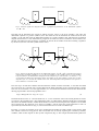
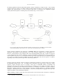
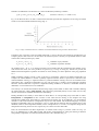
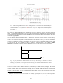


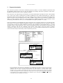


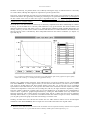


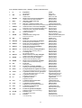


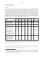

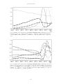


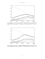
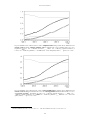


![Acctiva Professional 35 A [42,0426,0093,DE]](http://vs1.manualzilla.com/store/data/006740664_1-5560c8c3a0a8a7fe535db48be81090f9-150x150.png)