Download SC-88-02

H. Melenk, H.M. Möller *, W. Neun
On Gröbner Bases Computation on
a Supercomputer Using REDUCE
* FB Mathematik und Informatik
der Fernuniversität Hagen
D-5800 Hagen
Federal Republic of Germany-
Preprint SC 88-2 ( J a n u a r y 1988)
Konrad-Zuse-Zentrum für Informationstechnik;
Heilbrunner Straße 10; D-1000 Berlin 31
Herausgegeben vom
Konrad-Zuse-Zentrum für Informationstechnik Berlin
Heilbrunner Strasse 10
1000 Berlin 31
Verantwortlich: Dr. Klaus Andre
Umschlagsatz und Druck: Verwaltungsdruckerei Berlin
ISSN 0933-7911
Contents
1. Gröbner bases in R E D U C E 3.3
3
1.1
Gröbner bases and Buchberger's algorithm
3
1.2
Buchberger's algorithm in REDUCE 3.3
3
1.3
Cray computer usage for Gröbner calculations
4
1.4
Introduction of new facilities
4
2. Reflnement of Buchberger's algorithm and of its environment
5
2.1
The coefficient domains
5
2.2
Polynomial reductions
6
2.3
Extraction of power product factors
6
2.4
An additional criterion for detecting redundant pairs
7
2.5
Gröbner factorization
7
2.5.1
Factorization tree
7
2.5.2
Cancelling of redundant branches
8
2.5.3
Restrictions imposed by the application . . .
8
2.6
Modular coefficients
-
9
2.6.1
The direct method . .
9
2.6.2
The hybrid method
9
2.6.3
The parallel method
10
3. Technical improvements
10
3.1
Deferred branching for Gröbner factorization
10
3.2
Dynamic selection of coefficient domains . .
10
3.3
Data Representation
11
3.4
Polynomial reduction sets
11
4. Cray specific optimizations
12
4.1
Coefficient arithmetic
12
4.2
Exponent vector processing
12
5. Examples
5.1
12
A molecular structure
-
1
12
5.2
Modular Gröbner computations
14
5.3
Some comparisons
15
5.4
Calculations for large chemical reaction systems
16
Abstract
Gröbner bases are the main tool for solving systems of algebraic equations and
some other problems in connection with polynomial ideals using Computer Algebra Systems. The procedure for the computation of Gröbner bases in REDUCE
3.3 has been modified in order to solve more complicated algebraic systems of
equations by some general improvements and by some tools based on the specific
resources of the CRAY X-MP. We present this modification and illustrate it by
2
1. Gröbner bases in R E D U C E 3.3
1.1
Gröbner bases and Buchberger's algorithm
The concept of Gröbner bases, a special kind of bases for polynomial ideals,
was introduced by Buchberger in his thesis (1965) and developed in forthcoming
papers. Using Gröbner bases, many problems dealing with multivariate polynomials, especially algebraic equations can be solved. For a survey see Buchberger
(1985). We assume familiarity with the basic notions of Gröbner bases namely:
term ordering, leading term (It), leading coefficient (Ic), reduction modulo a finite
polynomial set, irreducibility modulo such a set, and S-polynomial. For polynomials over a field, we employ the same definition for Gröbner bases as Buchberger,
i.e. G is called a Gröbner basis if for any two / , g G G the S-polynomial S ( / , g)
reduces modulo G to 0. For polynomials over Zfi, we define Gröbner bases in the
same way but using pseudo-reduction for the S-polynomials as explained in 2.2.
This leads to a Gröbner basis notion, which is called in Möller (1988) a weak
Gröbner basis.
A Gröbner basis G is reduced if every / € G is irreducible modulo G \ {/}. In
case of polynomials over fields, every ideal possesses exactly one reduced Gröbner
basis F, where lc(f) = 1 for every / € F, cf. Buchberger (1985). Normalizing
every element of a reduced (weak) Gröbner basis F over 2Z by dividing it by its Ic,
we get such uniquely determined Gröbner basis, but now for the ideal generated
by F over Q instead over 2Z.
Given a finite polynomial set F generating an ideal I, Buchberger's algorithm consists essentially in calculating the S-polynomials, (pseudo-)reducing them modulo F to irreducible, so called H-polynomials, enlarging F by the nonzero Hpolynomials, removing from F such polynomials, whose It is a multiple of an It of
an other polynomial in F, and then continuing by calculating new S-polynomials
until no more S-polynomials exist leading to non-zero H-polynomials. At termination, F is a Gröbner basis of I. Buchberger (1985) gave criteria for predicting,
that some H-polynomials are 0. This allows to skip some S-polynomial calculations.
1.2
Buchberger's algorithm in R E D U C E 3.3
Buchberger's algorithm was implemented in the Computer Algebra System SAC2, see Böge, Gebauer, and Kredel (1986). It is based on the description of the
algorithm given by Buchberger (1985). The implementation of the algorithm
in REDUCE 3.3 by Gebauer, Hearn and Kredel is based on a variant, which
differs from the original Buchberger algorithm by a more efficient testing of the
criteria for omitting S-polynomial calculations and reductions. This variant is
described by Gebauer and Möller (1988) and also implemented in the meantime
in SCRATCHPAD II.
The REDUCE 3.3 implementation includes an internal package for the rhanip-
3
ulation of polynomials in a distributive representation. In this data structure a
polynomial is represented as linear sorted sequence of monomials. One advantage
of this kind of representation is the possibility to select an ordering of the monomials by ordering the terms, i.e. the power products of the variables x\,... , x n
in dependence of the desired application. In REDUCE 3.3, the following two
orderings are available.
The INV(erse) LEX(icographical) ordering:
(ai,...,a„) ^
~.{bi,-..,b„)
3i < n : (\/j < i : cij = bj) A a,- > fy
The I(nverse) T(otal) D(e)G(ree) ordering:
x ( a i , . . , a n ) >M^
x (6 1 ,...,6„)
(Ea«- > E *••)v (E a « = E hi A *<«~:-> >,.,„ X& »»>)
The INVLEX ordering is usefull for the solution of algebraic equations, see example 5.5. These two orderings are the same as in SAC-2, cf. Böge, Gebauer,
Kredel (1986), but different e.g. from those in Scratchpad II, cf. Jenks et al
(1986), such that reduced Gröbner bases in different systems, even if they are
normalized in the same way, can not be compared directly.
The REDUCE standard quotients are used as coefficients for the polynomials.
Standard quotients can be rational numbers or rational functions over variables
or formal functions (more general: kernels). So the algorithm in REDUCE 3.3
can be applied to polynomials over Q, the field of rational numbers, and to
polynomials over fields of rational functions.
1.3
Cray computer usage for Gröbner calculations
In 1986 REDUCE 3 was implemented for Cray 1 and Cray X-MP computers, Melenk and Neun (1987), based on Portable Standard LISP (PSL 3.4), see Anderson
et al. (1987) and Melenk and Neun (1986), and with Version 3.3 of REDUCE the
Gröbner package became available for these computers too. The objective was
to use the combination of REDUCE and the supercomputer for the enlargement
of the application range of Gröbner bases calculations towards 'larger' problems,
especially for the solution of systems of algebraic equations.
1.4
Introduction of new facilities
It soon became clear that the increased computing power alone was not sufficient
to reach our goal. So we started a four level approach:
4
- refinement of the Buchberger algorithm,
- improvement of the implementation,
- special tuning of basic package parts for the target machine and
- optimization of the underlying LISP.
The first two groups will be discussed in the following sections. They are machine
independent (in fact we developed the software using Sun and IBM computers
as workstations). The Cray specific parts will be mentioned only briefly.
2. Refinement of Buchberger's algorithm and of its
environment
2.1
T h e coefficient domains
We enlarged t h e range of applicable coefficient domains a n d fixed for a n y specific
coefficient d o m a i n a n a d e q u a t e normalization. In t h e field case all polynomials
are normalized internally t o have a leading coeffient 1, in the ring case (no general division available) t h e normalization reduces in general t h e contents of t h e
polynomials t o 1.
Normalization of t h e leading coefficients to 1
Q
rational numbers
Q(ai,...,aa)
rational functions in a\,...,
a, over Q
7LV
integers modulo a prime n u m b e r p
Content of polynomial coefficients normalized t o 1
7L
integer numbers of arbitrary length
2Z[ai,..., as]
polynomials in a\,...,
a, over 2Z
Other normalizations
M ( p i , . . . ,p3) Cartesian product of the prime fields ZPi,i.e.
M ( p i , . . . ,p s ) =
2Zn x . . . x ZPs. Here the leading coefficient is an s-tuple. It is
normalized to (1 mod p 1 } . . . , 1 mod pa), see 2.6.3.
H(p, f)
hybrid numbers, i.e. pairs of an integer modulo a given prime p
and a floating point number. The leading coefficient is here normalized to a hybrid number of type (1 mod p, i ) , x a floating point
number, see 2.6.2.
Experiments have shown, that for Gröbner basis calculations with non modular
coefficients the ring version of the algorithm is faster than the field version. Of
course, the calculations based on 2Z tend to produce bigger coefficients compared
to the Q applications, but this fact is not so important if a fast arithmetic is
available, see the statistics in 5.3. So the ring version is the default and'input
polynomials are converted from Q and Q(o,i,...,as)
to ZZ and Z5[ai,... ,a3]
5
by multiplying every coefficient of a polynomial with the 1cm of all coefficient
denominators (and using the identity a/1 = a for all a G 2Z or a € 2Z[a,i,... , a,]
resp.).
2.2
Polynomial reductions
A single reduction step modulo a finite set G of non-zero polynomials reduces a
polynomial / to a polynomial h := f — tg, with g 6 G, t a monomial, such that
the monomial m in / with lt(m) = lt(t)-lt(g) is canceled by t-g, but h contains in
addition some more monomials of lower order. A pseudo-reduction step modulo
G reduces / to c • / — t • g, with g G G, t a monomial and c a constant coefficient,
such that again the monomial m with lt(m) = lt(t) • H(g) in / is canceled. This
pseudo-reduction is installed in addition to the existing reduction and used for
polynomials over 2Z and 2Z[ax,..., as].
For testing the efficiency of reduction procedures, we installed also the so called
It-reduction. This is also a reduction in the sense explained before, but the
monomial m in / which is canceled must be maximal: H(m) — lt(f).
This
reduction is already sufficient in Buchberger's algorithm for obtaining a Gröbner
basis, see for instance Möller (1988). However, as our tests in 5.3 indicate, the
It-reduction is in general slower.
As an optional feature we can start the algorithm by first reducing cyclically
the input polynomials with themselves, i.e. reduce each f (~ F modulo {g 6
F\lt(g) < /<(/)•} beginning with an / with maximal lt(f) and resulting in a
reduced polynomial set F', which can be reduced again in the same manner, etc.
Such a specific reduction phase can eliminate redundancies more efficiently than
the main algorithm. A similar prereduction takes place, immediately before a
Gröbner basis calculation for a subproblem as described in 2.5 is started.
2.3
Extraction of power product factors
When Gröbner bases are needed only for the solving of a set of algebraic equations, multiplicities of zeros may be ignored. Therefore multiple factors of a
polynomial may be reduced to simple ones by polynomial division. We installed
for the situation, when such multiple factor is a power product, a procedure
following a proposal of Davenport (1987). If / has a power product factor,
f =
x\xxk2*---xkr?g,
f =
xl{x%---x,£g,
then / is replaced by
with /,• := 1 if k{ > 1, and /,- := 0 if &,• = 0, i = 1 , . . . , m. (The new / has the same
zeros as the old one but the multiplicity is reduced at all hyperplanes x,- = 0,
where the old / vanishes with multiplicity greater than 1). This causes, that the
algorithm calculates no longer a Gröbner basis of the ideal generated by the input
polynomials but of an ideal between this ideal and the radical ideal, which consists
6
of all polynomials vanishing at the common zeros of the input polynomials. Such
power product factor can be detected easily in the distributive representation:
its exponent vector is the vector of the componentwise minima over all exponent
vectors. This vector is computed during the normalization of each polynomial
and held in its data structure.
2.4
A n additional criterion for detecting redundant pairs
If two polynomials pi and j»2 a r e known to have a common factor g,
Pi = 9fu P2 = 5/2,
and if
gcd{i<(/iy*(/2)} = i,
then we know in analogy to criterion 1 of Buchberger (1985), that the S-polynomial
from pi and pi will reduce to 0. This criterion will be used for power products
divisors g (see 2.3). This gives a new criterion for omitting superfluous reductions
cf. Buchberger (1985) or Gebauer and Möller (1988). It can lead in cases, where
many polynomials with common factors occur, to a better performance of the
algorithm.
2.5
Gröbner factorization
For solving a system of algebraic equations
/ 1 (x) = 0 , . . . , / r ( x ) = 0,
this means, for finding Z(fi,...,
/ r ) , the set of common zeros of all polynomials in
Ideal(fi,...,
/ r ) , Gebauer and Möller tested in a preliminary version of REDUCE
3.3 the following procedure. If in the algorithm a polynomial h G Ideal(fi,...,
fT)
'is found, which can be factorized into
h = hi • . . . • / i m ,
then Z(fi,...,
/ r ) is the union of the sets
Z(fi,...1fr,hk),k
=
l,...,m.
Thus when the algorithm did actually compute h, it branches. For each hk in
place of h it is continued resulting in the Gröbner bases for Ideal(fi,...,
/ r , hk), k =
1 , . . . , m. This factorization of the Gröbner basis calculations is also investigated
by Davenport(1987).
2.5.1
Factorization tree
In the present package we have elaborated this approach by consequently testing
all polynomials (input, intermediate and result) for power product factors and
7
by calling the REDUCE factorizer. If a factorization is detected, the state of the
algorithm is encapsulated and for each of the factors a subproblem is generated
and stacked into a list of open problems. Of course, the set of all such problems
constitutes a tree with the initial problem of computing Z(f\,...,
fr) as root.
2.5.2
Cancelling of redundant branches
Consider the subproblem for calculating Z{gx,..., gs) and let h £ Ideal(gi,...
possess a factorization
h — hi •... • hm.
,g3)
yielding the subsequent subproblems for calculating the sets Z(gx,..., g3, hk), k =
1,...., m. It may turn out, that Z(gx,..., gs, hk) is void, i.e. 1 G Ideal{gx,...,
gs, hk),
or that Z(gx,..., ga, hk) is contained in a previously computed set of zeros, such
that its computation is superfluous. In order to avoid such superfluous sets
of zeros, we associate to every problem a set of polynomials, starting with
the empty set for the initial problem. If the set P is associated to the problem of calculating Z(gx,... ,g3), then P is associated also to the problem of
calculating Z(gx,... ,ga, hx). If P' is associated to the problem of calculating
Z(gi,...,g„,
hk), 1 < k < m, then P' U {hk} is associated to Z{gx,... ,gs, hk+i).
This gives the following criterion
( C ) : If we start calculating the Groebner basis of Ideal(g\,... ,g3) and detect
a polynomial in it, which belongs also to the polynomial set associated to
Z{g\, • • •, ga), then we stop the Gröbner basis calculation and remove the
problem of computing Z{gx,..., gs) from the set of open problems.
The usage of this criterion is justified by the following reason. If / belongs to
the polynomial set associated to Z(gx,..., g3) and / G Ideal(g\,...,
g3), then a
j < s exists by construction, such that / and gj+1 are both factors of gj, f the
lower indexed factor. Since / € Ideal(gu . . . , g3), we have Ideal(g\,...,
gj, f) C
Ideal(gi,...,
g3). Therefore Z{g\, ...,g3) Q Z{g\,..., gj, f) holds, i.e. the problem of computing Z{g\,...,g3)
is superfluous:^
2.5.3
Restrictions imposed by the application
In some applications only solutions are of interest which fullfill certain algebraic
restrictions. In some examples, we are only interested in nonnegative (real)
solutions. (For instance negative mass makes no sense.) So we implemented a
hook for the used to decide via a procedure whether a polynomial violates these
restrictions. As a standard procedure the testing for nonnegative solutions is
present and can be activated on request
- A polynomial J2 a^i 1 * • • •' xnn + a o with all a,- and ÜQ positive has no zero
( z i , . . . , xn) with all X{ nonnegative (and real). So the calculation branch
can be cancelled.
8
- A polynomial J2 o-i^'i • • • • • x%n without an absolute term a0 and with all
a; positive can vanish only if all of its summands vanish. This is possible
only if in any summand at least one variable is zero. In most cases there
are several possible combinations. The list of combinations play the same
role as a factorization and is handled in the same manner.
Although this approach is independent from factorization, it plays its most important role in this context: the main problem of factorization is the fight against
the great number of branches. The earlier a polynomial without (componentwise) nonnegative zeros is detected in a branch, the earlier the computation in
this branch may be interrupted (at the expense of an additional branching or a
complete cancellation of the branch).
2.6
Modular coefficients
Modular techniques are helpful, when the coefficients of the output polynomials
are expected to be of the same (moderate) size as the input coefficients, but
intermediate polynomials with big coefficients occur. We have three methods for
computing a Gröbner basis over the rationals by means of modular techniques.
2.6.1
T h e direct m e t h o d
Take a (sufficiently big) prime p. Transform each input polynomial to a polynomial over 2ZP by substituting its coefficient c/d by a, such that c = a-d mod p, 0 <
a < p. Compute a reduced Gröbner basis over 2ZP with each leading coefficient
normalized to 1. Reconstruct each Gröbner basis coefficient a mod p to a rational
number by means of the algorithm of Wang (1981). The resulting polynomials
constitute the reduced normalized Gröbner basis over Q, if p is a sufficiently big
lucky prime.
2.6.2
T h e hybrid m e t h o d
Many polynomials come from scientific applications, where the coefficients are
only approximations to some 'real life' quantities. So the coefficients are typically floating point numbers. On the other hand Buchberger's algorithm requires exact coefficients. Therefore we compute via REDUCE rational numbers
approximating the floating point values and from that we produce a modular
number. The modular number and the floating point value then are paired for
Buchberger's algorithm to a hybrid number. The arithmetic is defined componentwise. The modular number now controls Buchberger's algorithm allowing
exact calculations, while the floating point values are calculated as side effects.
At termination of the algorithm, the polynomials with the modular part of the
hybrid numbers as coefficients constitute a Gröbner basis. The polynomials with
the float number parts as coefficients are then expected to be approximations to
the Gröbner basis polynomials of the initial 'real life' problem. Because we do
9
not reconstruct the 'true values' from the modular number, the prime number
can be of moderate size.
2.6.3
The parallel method
As proposed by Knuth (1981), each integer a mod px-.. .-ps with pairwise different
primes p,-,i = l , . . . , s , can be represented uniquely by an s-tuple ( a i , . . . , a a )
with a = a,- mod pi and given the a,'s the integer a can be reconstructed by the
Chinese remainder theorem. Therefore, we proceed as in 2.6.1 in order to find
Gröbner bases over ZPi. The arithmetic operations for these tuples are defined
componentwise
( a i , . . . , a s ) • ( 6 i , . . . , b3) = (aj • &i,..., a„ • b3)
With • G {+modi
modi *mod> / m o d ) •
When one component of a nonzero tuple is 0, then the corresponding p,- is unlucky
and henceforth ignored for the reconstruction of the integer a by the Chinese
remainder theorem. In that case, the reconstructed a by the Chinese remainder
theorem is at most exact modulo px •... • p3/pi-
3. Technical improvements
3.1
Deferred branching for Gröbner factorization
When doing Gröbner factorizations as described in 2.5 for a problem with many
variables and a 'sparse' coefficient pattern, we detected, that different branches
starting from one h = h\ • ... • hm had to do the same calculations for those
polynomials depending only on variables different from those in hx,..., hm. So
we implemented a delay: if a branching point is encoutered, the algorithm sets
aside the factors and continues the calculations for those pairs with leading terms
in variables disjoint to those of h\,..., hm. Here new factorizations can be found,
which are handled in the same way. Finally we have several levels of factorization
at the same time giving a rich information for the configuration of subproblems.
In most cases factors themselves are of very low degree and so we do an additional
reduction of all polynomials in one branch with its creating factors, which gives
a further reduction of problem size.
3.2
D y n a m i c selection of coefficient domains
The interface for the coefficient manipulation of the distributive polynomials was
redesigned completely. So it now has one separate package for each coefficient
domain; one of them is the interface to the REDUCE standard quotients (SQ).
Others are those for Q, Zp, H(p, / ) , M ( p l 5 . . . , p 4 ). Additional packages can be
plugged in easily. As default the algorithm expects coefficients in the most general
domain SQ. In its starting phase it does a general data type analysis and selects
automatically the simplest arithmetic for the given problem.
10
This is an efficient mixture of static and dynamic typing: the type analysis
is done dynamically once in the starting phase. In the main working phase
there is no more type checking because then all switches are already set. This
procedure is justified by the fact, that the type analysis is very small compared
with Buchberger's algorithm itself.
3.3
D a t a Representation
In the original version polynomials were represented as standard lists. This organization is efficient for the manipulation, but it consumes too much storage if
large problems with thousands of intermediate polynomials are handled and it
does not allow to link additional information to the individual polynomials.
So the polynomials now are embedded in an object oriented structure, which allows several different memory organizations with compatible generic access methods at the same time. Each polynomial posesses a property list for descriptive
slots, e.g. a name of the polynomial for trace purposes, its known factors, the
subspace of its variables. Because of the object oriented approach different memory organizations can be used at the same time. By default two organizations
are active: one simple (in fact the traditional list in an encapsulated version)
for temporary intermediate results and a compressed representation for those
polynomials which will survive local calculations (e.g. the H-polynomials). So
calculations with many intermediate H-polynomials are possible in memory. If
the memory limit is exceeded, an additional organization is available which places
polynomials on secondary storage. The only inference between the algorithm and
the memory organization is the explicit marking of a polynomial to be of the 'survival' type.
3.4
Polynomial reduction sets
It turned out, that Gröbner bases calculations are more efficient, when we distinguish between the set G of all polynomials (from input and H-polynomial
calculation) and the set F obtained from G by cancelling redundant elements; F
is finally the reduced Gröbner basis whereas G is used in place of F for reducing
the polynomials during the algorithm as sketched in 1.1. If G contains a great
number of polynomials, the search for a candidate for the reduction may require
some time. Therefore G is stored as a tree, which reflects the structure of the It
part such that the optimal polynomial for a given reduction step can be found
by 'addressing' it.
11
4: Cray specific optimizations
4.1
Coefficient a r i t h m e t i c
By analyzing the run-time behaviour of the original package it soon became
clear, that the heavy usage of arbitrary precision integer arithmetic was one
main bottleneck. So we rewrote the PSL 'big' package now using the Cray vector
hardware. This gave a significant run-time reduction and stressed the superiority
of 2Z based computations compared to Q based computations.
An obviously 'native' area for a vector computer are the 2SP1 x . . . x ZSPa coefficients, where the transformation from the algorithmic level to the machine level
is (almost) obvious. The operations + , —, * can be mapped to one vector instruction cycle each, doing the basic integer operation and adjusting components
with overflow (masking out non overflow components). The pseudo-division is a
little bit more complicated because the number of loops needed by the extended
Euclidean algorithm depends of the magnitude of the input values; here the loop
is performed until all values are finished; the components which are ready earlier
are ruled out by masking instructions.
4.2
E x p o n e n t v e c t o r processing
The processing of exponent vectors is the second bottleneck of distributive polynomial processing. Exponent vectors traditionally are stored as lists of (small)
integers. Most of the processing time spent with exponent vectors is needed for
the comparison (term ordering). The list structure is very adequate for this type
of operation: two vectors are compared from 'left to right' breaking when the
first non equal position is found. Total degree requires additionally a horizontal
sum over the vectors. We have improved this type of processing by exploiting the
pipelined memory access of the vector computer: while processing two exponent
vectors four items are loaded in parallel in each cycle, the two elements to be
processed and the two pointers to the rest of the structures.
5. Examples
5.1
A molecular structure
We received a set of algebraic equations
fi{y\,yi,yz)
= o , » = o , . . . , 3,
from A. Dress (1987). It describes the molecular structure of a cyclic carbon
are
hydrogen molecule with six nodes. The polynomials / 0 , f\,f2,h
given by
12
/o:=
0
1
1
1
1
1
1
1
0
1
8/3
yi
8/3
l
1
1
0
1
8/3
y2
8/3
1
0
1
8/3
y3
8/3
1
0
1
8/3
0
1
1
0
1 8/3
1
Vi
1 8/3
1
1
V2 8/3 1
8/3 V3 8/3
,/i==
0
1
1
l
1
1
1
0
1
8/3
yi
8/3
l
l
0
1
8/3
y2
1
8/3
1
0
1
8/3
1
1
Vi 8/3
8/3 y2
1
0
1
8/3
1
0
foivuViiVs) : = /i(?/2,y3,yi),
/ 3 ( y i , y 2 , y 3 ) : = / i ( y 3 , y i >y2)-
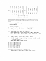
In order to find the common zeros Z(fQl / j , / 2 , fj) of Ideal(f0, / l 5 / 2 , / 3 ) , we proceed as described in 2.5. Buchberger's algorithm is performed with the following
features:
- inverse lexicographical ordering
- integer coefficients
- Gröbner factorization.
The factorization produces eight Gröbner bases. Z ( / o , / i , / 2 , / 3 ) is the union of
the sets £((?,-), i = 1 , . . . , 8, where the Gröbner bases G\,..., G% are
Gi:
{3 y i y 2 + 3y a y 3 - 22yx + 3y 2 y 3 - 22y2 - 22y3 + 121,
27y x y| - 198 yi y 3 + 7 5 y i + 27y 2 y| - 198y2y3 + 75y2 - 198y| + 1164y3 + 250,
81y 2 y 2 - 594y22y3 + 225y2 - 594y2y2 + 3492y2y3 + 750y2 + 225y32 + 750y3 - 14575},
G2:
{27360yx + 27360y2 - 1377y| - 2925y| + 59685y3 - 304855,
82080y2. - 4131y 2 y| - 8775y 2 y| + 179055y2y3 - 914565y2 + 30699y| + 79695y2
- 1192215y3 4- 2952125,
243y£+.540yf - 9630y| + 25500y3 - 26125},
G3:{3y1-ll,9y2-25,3y3-ll},
G4:{3y1-ll,3y2-ll,3y3-ll},
G5:{9y1-25,3y2-ll,3y3-ll},
G 6 : { 3 y i + 5 , 3 y 2 - 1 9 , 3 y 3 + 5},
G 7 : { 3 y i 4 - 5 , 3 y 2 + 5,3y 3 + 5},
G 8 : { 3 y 1 - 1 9 , 3 y 2 + 5,3y 3 + 5}.
Denoting the three polynomials of G\ by #i,<72)<73, we find
76800^ = (81y 2 y 3 - 369y22 - 594y2y3 + 1842y2 + 225y3 - 1375)^2
13
+(123 y i + 123y2 - 21ym
- 27y2y3 + 198y3 - 614)^3
i.e. gx vanishes at the common zeros of g2 and g3. Using y3 for a free parameter,
the common zeros of <7i,<72,<73 are hence (yi,y2,y3) with
yi:
~
99y| - 582y3 - 125 ± y/Ä
_ 99y| - 582y3 - 125 T V&
27y2 - 198y3 + 75
'V2 : ~
27y32 - 198y3 + 75
'
where A := 7776yJ - 107136y| + 489024y| - 835200y3 + 380000.
The polynomials of G2 have exactly eight zeros (y1} y 2 , y 3 ) in common. The third
component y3 is a zero of the irreducible polynomial
243y3 + 540y^ - 9630y^ + 25500y3 - 26125
(i.e. four different choices), the second component y2 is then determined by
82080y| - 4131y2y* - 8775y2y^ + 179055y2y3 - 914565y2 + 30699y| + 79695y|
-1192215y 3 + 2952125 = 0
(i.e. two choices for fixed y 3 ), and the first component yx is determined for given
y2 and y 3 by
27360yi + 27360y2 - 1377y| - 2925y| + 59685y3 - 304855 = 0
The common zeros of the last six bases can be read off immediately.
The overall time for computing the eight Göbner bases is
3.5 sec (using a Cray X-MP 2400),
104 sec (using a SUN 3-260).
In this example, long integer coefficients occured in the intermediate computations.
5.2
Modular Gröbner computations
As example for the efficiency of vector hardware usage a test calculation may
serve: An example in Böge et al.(1986) originating from W. Trinks produces
moderate long integer coefficients and so we have calculated it with 63 component modular vectors with different technical supports: sequential processing of
vectors (compatible version of this arithmetic) and processing by Cray vector instructions. Of course, this is no real application: the problem and the coefficients
are too small and so the computation of the reduced normalized Gröbner basis
w.r.t. the INVLEX ordering is totally dominated by the reconstruction effort.
TRINKS1 (6 polynomials in 6 variables over
M(p1,..,p63))
sequential processing
5.8 sec
usage of vector hardware
0.7 sec
Reconstruction of coefficients:
8.5 sec
14
Another example in Böge et al.(1986) originating from
a case where a computation with lexicographical order
Cray installation we computed the Gröbner basis over
version is much more efficient, because the Gröbner
coefficients (300decimal digits).
ROSE (3 polynomials in 3 variables)
M.Rose was mentioned as
was impossible. With our
7Z>. But here the modular
basis has some very long
ITD :
see 5.3
INVLEX over Z:
2288 sec. Cray X-MP in a job with
2.5 million (64-bit-)words of memory.
INVLEX over M(536870909):
92 seconds Cray X-MP
INVLEX over M(pi,-.,Pi3o):
148 sec. Cray X-MP (for Buchberger's
algorithm) plus 112 sec. Cray X-MP (for
the coefficient reconstruction)
Of course, the single modular computation indicates as result only the monomial
layout. It has the aspect of a 'pioneer' computation. The calculation with coefficient vectors of length 120 modulo primes of moderate size (less than 21 bits each)
allows the reconstruction of the true basis coefficients; when normalized by REDUCE common denominator technique these are identical with the coefficients
calculated over 2L. Eight of the 120 primes were unlucky; they could not take
part in the reconstruction. It turned out, that 100 primes of this moderate size
are the minimum for the reconstruction of the coefficients. It should be noted
here, that because of the vector hardware the time of Buchberger's algorithm
with 120 modular coefficients is not much slower than that with one modulus;
in fact the additional time needed for the vector version has its origin mainly in
the fact that more dynamic memory is wasted (additional garbage collections).
5.3
Some comparisons
For comparisons we have done some calculations with examples listed in Böge
et al. (1986). We stress, that our Gröbner package is designed for 'real life'
applications requiring the power of a super computer. Therefore we omitted
the tests of too simple examples. But for economical reasons, we also did not
try all hard problems of Böge et al. We present six medium range problems as
candidates for testing the various features of an implementation. The following
statistics demonstrate the influence of the options on the computing time. All
these examples are no cases where there is an urgent need for the Cray power.
All computing times are given in seconds of a Cray X-MP; the time needed for
garbage collections during the computations is included (the memory was limited
to 1 million words).
15
Bas
D=Q
Lorg
Prered
ltred
Fact
Orig
TRINKS1
0.3
6.3
0.3
0.4
0.2
2.1
17.0
GERDT
13.6
31.1
12.5
13.5
23.1
9.8
32.1
HAIRER3
12.9
14.8
11.7
12.6
136.0
> 999
38.1
KATSURA4
0.8
2.6
0.8
0.8
3.0
1.7
6.0
ROSE itdg
2.1
8.9
1.6
2.1
4.2
26.9
20.9
GÖNNET
1.4
1.4
0.9
1.0
2.3
0.8
1.1
Meaning of the columns:
B a s : A 'basic' package of options: Domain = Z, polynomials compressed, no
prereduction of input, full reduction, no factorization. The subsequent
columns (except the last one) differ from this column by only one modification each.
D = Q : Usage of rational numbers instead of integers.
Lorg: Switching off internal compression (cf. 3.4).
Prered: Prereducing of the input polynomials.
Itred: Only It-reduction.
Fact: Factorizing enabled.
Orig: usage of the original Gröbner package of REDUCE 3.3
The statistics give the following result: Domain 7Z is 'faster' than Q in almost all
cases (except the last one, where it is equal). The internal compression causes in
general a neglegiable overhead for these medium range problems; only the last
case suffers explicitly from this option; it causes an almost uniform overhead with
the larger problems and one should take into account, that avoiding a memory
overflow is a question of computability at all. The prereduction makes sense in all
cases: if it produces no time saving, it costs not much. Only one case was found,
where restricting the reduction to the It-parts gives a tiny speedup. The benefit
of factorization varies from problem to problem very much; if a factorization is
found, it can shorten the calculation (and it gives much better usable results); if
not, it requires an important additional computing time.
5.4
Calculations for large chemical reaction s y s t e m s
These examples have their origin in a system of ODE's describing chemical reaction systems. Up to 60 polynomials in up to 60 variables (number of variables and
number of equations not necessarily equal). The polynomials are extracted from
the ODE system without further preprocessing. Their maximal degree is 3. The
original coefficients are floating point numbers. Most polynomials cite only a few
, number of variables ('sparse' system). Using the original algorithm the bigger
16
problems consume all available resources in an exploding manner without producing any result. Therefore we used the following configuration of Buchberger's
algorithm.
- reducing the input polynomials with themselves as long as It parts can be
cancelled (actually 5 cycles), cf. 2.2.
- cancellation of multiple power product factors, cf. 2.3.
- factorization on the base of power product factors, cf. 2.5 .
- inverse total degree ordering.
- hybrid coefficients, cf. 2.6.2.
Using this configuration, we find a set of (partial) Gröbner bases. Some of these
bases have a very simple structure, e.g. only linear polynomials, such that the
solution can be read off immediately.
The following example HAVC4 was given to us by P. Deuflhard (1986). It consists
of 50 polynomials in 37 variables. The longest polynomial has 31 terms. Some of
the polynomials have only 1 term. We found hundreds of partial Göbner bases
which were all of the same simple structure, such that their common zeros could
be detected without additional computations. The 'rate' on the Cray X-MP was
'one base per 4 CPU seconds'. An inspection gave, that most of these bases have
only solutions with at least one negative component. Therefore the
- restriction for nonnegative values, cf. 2.5.3,
is imposed. This reduces the amount of solutions and of calculation branches
dramatically. The algorithm now terminates in 358 seconds (overall computing
time inch garbage collections ) on the Cray giving 330 partial Gröbner bases.
A postprocessing analyse detects that most of these solutions are still redundant
in the sense, that they describe a subspace of other solutions. The final number
of independent solution spaces is eleven.
17
References
J . W . A n d e r s o n , W . F . Galway, R . R . Kessler, H . M e l e n k , W . N e u n : Implementing and Optimizing Lisp for the Cray, IEEE Software, July 1987.
W . B ö g e , R. Gebauer, H. Kredel: Some Examples for Solving Systems of Algebraic Equations by Calculating Groebner Bases, J. Symb. Comp. 1986,
vol.2, pp. 86 - 98.
B. Buchberger: Ein Algorithmus zum Auffinden der Basiselemente des Restklassenrings nach einem nulldimensionalen Polynomideal, Ph.D. thesis, Innsbruck, 1965.
B. Buchberger: Gröbner bases: An algorithmic method in polynomial ideal theory. (In: Multidimensional Systems Theory, ed.: N.K. Böse) D. Reidel
Publ. Comp. 1985, pp. 184 - 232.
J. H. Davenport: Private communication
1987.
P. Deuflhard: Private communication 1987.
A. Dress: Private communication
1987.
R. Gebauer, H . M . Möller: On an installation of Buchberger's algorithm. To
appear in J. Symb. Comp. 1988.
A.C.Hearn: REDUCE
1987.
User's Manual, Version 8.3, The Rand Corporation,
R. Jehks et al.: Scratchpad II, an experimental computer algebra system, abbreviated primer and examples, IBM Thomas Watson Research Center,
Yorktown Heights, N.Y. 10598, 1986.
D.E. Knuth: The Art of Computer Programming Vol 2: Seminumerical Algorithms, 2nd edition, 1981.
H.M.Möller: On the construction of Gröbner bases using syzygies, to appear
in J.Symb. Comp. 1988.
H. Melenk, W. Neun: REDUCE Users Guide for Cray 1/ X-MP Series Running COS, Konrad-Zuse-Zentrum Berlin, Technical Report T R 87-4 , 1987.
H. Melenk, W . N e u n : Usage of Vector Hardware for LISP Processing, KonradZuse-Zentrum Berlin, 1986.
P. Wang: A p-adic algorithm for univariate partial fractions, Proc. SYMSAC'81,
ACM, pp. 2 1 2 - 2 1 6 , 1981.
18